The Estimation of Causal Effects by

Difference-in-Difference Methods Michael Lechner September 2010 Discussion Paper no. 2010-28

Department of Economics University of St. Gallen

Editor: Martina FlockerziUniversity of St. Gallen Department of Economics Varnbüelstrasse 19 CH-9000 St. Gallen Phone +41 71 224 23 25 Fax +41 71 224 31 35 Email vwaabtass@unisg.ch

Publisher: Electronic Publication:

Department of EconomicsUniversity of St. Gallen Varnbüelstrasse 19 CH-9000 St. Gallen Phone +41 71 224 23 25 Fax +41 71 224 31 35 http://www.vwa.unisg.ch

The Estimation of Causal Effects by Difference-in-Difference Methods 1

Michael Lechner2

Author’s address: Prof. Dr. Michael LechnerSwiss Institute for Empirical Economic Research (SEW-HSG) Varnbüelstrasse 14 CH-9000 St. Gallen Phone +41 71 224 2320 Fax +41 71 224 2302 Email Michael.lechner@unisg.ch Website www.sew.unisg.ch/lechner

1 This project received financial support from the St. Gallen Research Centre of Aging, Welfare, and Labour

Market Analysis (SCALA).The paper was presented at the econometrics breakfast at the University of St. Gallen and benefited from comments by seminar participants. I thank Christina Felfe, Alex Lefter, and Conny Wunsch for carefully reading a previous draft of this manuscript, Patrick Puhani for an interesting discussion on some issues related to limited dependent outcome variables, and Jeff Smith for additional useful references. The usual disclaimer applies.

2 Research Associate of ZEW, Mannheim, and a Research Fellow of CEPR, London, CESifo, Munich, IAB, Nuremberg, IZA, Bonn, and PSI, London.

Abstract

This survey gives a brief overview of the literature on the difference-in-difference (DiD)

estimation strategy and discusses major issues using a treatment effect perspective. In this

sense, this survey gives a somewhat different view on DiD than the standard textbook

discussion of the difference-in-difference model, but it will also not be as complete as the

latter. This survey contains also a couple of extensions to the literature, for example, a

discussion of and suggestions for non-linear DiD as well as DiD based on propensity-score

type matching methods.

Keywords

Causal inference, counterfactual analysis, before-after-treatment-control design, control

group design with pretest and posttest.

JEL Classification

C21, C23, C31, C33.

1

1. Introduction

The Difference-in-Difference (DiD) approach is an econometric modelling strategy for

estimating causal effects. It is popular in empirical economics, for example to estimate the

effects of certain policy interventions and policy changes that do not affect everybody at the

same time and in the same way, but it is used also in other social sciences.1 DiD is an

attractive empirical strategy in cases when controlling for confounding variables is not

possible and attractive instruments are not available and at the same time pre-treatment

information is available though. 2 It is based on at least four (sometimes overlapping)

subgroups. Three of them are not affected by the treatment. Usually, 'time' is an important

variable to distinguish the groups.3 Besides the group who already received the treatment

(post-treatment treated), these groups are the treated prior to their treatment (pre-treatment

treated), the non-treated in the period before the treatment occurs to the treated (pre-treatment

nontreated), and the nontreated in the current period (post-treatment non-treated).4 The basic

idea of this identification strategy is that if the two treatment and nontreated groups are

subject to the same time trends, and if the treatment has no effect in the pre-treatment period,

1 In other social sciences the DiD approach is also used under the label of "untreated control group design with independent

pretest and posttest samples" or "control group design with pretest and posttest". See, for example, Cook and Campbell

(1979), Rosenbaum (2001), and Shadish, Cook, and Campbell (2002) for further references.

2 Following the literature, I call the event for which we want to estimate the causal effect the treatment. The outcome

denotes the variable that will be used to measure the effect of the treatment. Outcomes that would be realised if a specific

treatment has, or would have been applied are called potential outcomes. A variable is called confounding if it is related to

the treatment and the potential outcomes such that a mean comparison of observed outcomes for different levels of the

treatment would be an inconsistent estimator for the corresponding average effects. A variable is called an instrument if it

influences the treatment but not the potential outcomes.

3 As the concept of time is only used to define a group that is similar to the treated group with respect to relevant

unobservable variables and who have not (yet) participated, any other characteristic may be used instead of time as well,

as long as the formal conditions given below are fulfilled.

4 When a data set is available in which everybody is observed in all periods, there will be just two groups with outcomes

measured before and after the treatment.

2

then an estimate of the 'effect' of the treatment in a period in which it is known to have none

can be used to remove the effect of confounding factors to which a comparison of post-

treatment outcomes of treated and nontreated may be subject to. Another way to phrase this is

to say that we use the mean changes of the outcome variables for the nontreated over time and

add this to the mean level of the outcome variable for the treated prior to treatment to obtain

the mean outcome the treated would have experienced if they had not been subject to the

treatment.

This survey presents a brief overview of the literature on the difference-in-difference

estimation strategy and discusses major issues mainly using a treatment effect perspective

(and language) that allows, in our opinion, more general considerations than the classical

regression formulation that still dominates the applied work. In this sense, this survey might

give a somewhat different perspective than the standard text book discussion of the

difference-in-difference model, but it will also not be as complete as the latter. Thus, this

paper is more of a complement than a substitute to the excellent text type discussions of the

difference-in-difference approach that are already available (e.g. Angrist and Pischke, 2009,

Blundell and Costa Dias, 2009, and Imbens and Wooldridge, 2009).

This paper focuses on the case of two differences only, although the basic ideas of

difference-in-difference (DiD) estimation could be extended to more than two dimensions to

create difference-in-difference-in-difference-in-… estimators.5 However, the basic ideas of

the approach of taking multiple differences are already apparent with two dimensions. Thus,

5 For example, Yelowitz (1995) analyses the effects of losing public health insurance on labour market decisions in the US

by using Medicaid eligibility that varies over time, state and age (of the child in the household). Another example for a

triple difference is the paper by Ravallion, Galasso, Lazo, and Philipp (2005) who analyse the effects of a social

programme based on a comparison of participants with nonparticipants and ex-participants.

3

we refrain from addressing these higher dimensions in this survey to keep the discussion as

focused as possible.

The outline of this survey is as follows: The next section gives a historical perspective

and discusses some interesting applications. Section 3, which is the main part of this survey,

discusses identification issues at length. Section 4 concerns DiD specific issues related to

estimation, including a discussion of propensity score matching estimation of DiD models.

Section 5 discusses some specific issues related to inference and section 6 considers important

practical extensions of the basic approach. Section 7 concludes. Some short proofs are

relegated to an technical appendix.

2. The History of DiD

In our days the method of difference-in-difference estimation is well established and,

although there are a couple of open issues, the main components of this approach are well

understood.6 The first scientific study using explicitly a difference-in-difference approach

known to the author of this survey (and mentioned by Angrist and Pischke, 2009) is the study

by Snow (1855). Snow (1855) was interested in the question whether cholera was transmitted

by (bad) air or (bad) water. He used a change in the water supply in one district of London,

namely the switch from polluted water taken from the Themes in the centre of London to a

supply of cleaner water taken upriver. The basic idea of his study is described by a quote from

the introduction to (the reprint of) his book by Ralph R. Frerichs: "… Another investigation

cited in his book which drew praise for Snow was his recognition and analysis of a natural

6 Expositions of this approach at an advanced textbook level are provided for example by Meyer (1995), Angrist and

Krueger (1999), Heckman, LaLonde, and Smith (1999), Angrist and Pischke (2009), Blundell and Costa Dias (2009), and

Imbens and Wooldridge (2009). For one of the rather rare treatments of this topic in the statistics literature see Rosenbaum

(2001).

4

experiment involving two London water companies, one polluted with cholera and the other

not. He demonstrated that persons who received contaminated water from the main river in

London had much higher death rates due to cholera. Most clever was his study of persons

living in certain neighbourhoods supplied by both water companies, but who did not know the

source of their water. He used a simple salt test to identify the water company supplying each

home. This reduced misclassification of exposure, and provided him with convincing

evidence of the link between impure water and disease." Obviously, using close

neighbourhoods is clever, as they are probably exposed to similar air quality. It is worth

adding that Snow also had data on death rates in those neighbourhoods prior to the switch of

water supply. He used them to correct his estimates for other features of these neighbourhoods

that could also lead to differential death rates. In that way, the first difference-in-difference

estimate appeared, and, because of its high credibility coming from Snow's (1855) clever

research design, it had an important impact for public health in a scientific as well as in a very

practical, life-saving way.

Later on this type of approach became relevant also for other fields, like psychology

for example. Rose (1952) investigated the effects of a regime of 'mandatory mediation' on

work stoppages by a difference-in-difference design, as can again be seen from a quote from

his article: "To test the effectiveness of mandatory mediation in preventing work stoppages, it

is necessary to make two simultaneous comparisons: (1) comparisons of states with the law to

states without the law; (2) comparisons of the former states before and after the law is put into

operation. The first comparison can be achieved by taking percentages of each of the three

states to the total United States, for the measures used. The second comparison can be

achieved by setting the date of the passage of the law at zero for each of the states. Figure 1

indicates both comparisons simultaneously. …" (Rose, 1952, p. 191).

5

In economics, the basic idea of the difference-in-difference approach appeared early.

Obenauer and von der Nienburg (1915) analysed the impact of a minimum wage by using an

introduction of the minimum wage in the state of Oregon that, for a particular group of

employees, led to higher wage rates in the largest city, namely Portland, compared to the rest

of the state. Therefore, the authors documented the levels of various outcome variables for the

different groups of employees in Portland before and after the introduction of the minimum

wage (in the retail industry) and the respective changes observed in another city in the state,

Salem.

Another early application in economics is by Lester (1946). He was concerned with

the effects of wages on employment and used a change in the minimum wage. He based his

analysis on a survey of firms that had operations in both the northern and the southern US

states. His idea was to compare employment levels before and after various minimum wage

rises for groups of firms with low average wages to groups of firms with higher wages levels,

whose wage bills were naturally only mildly affected, if at all, by the rise in the minimum

wage.

An aspect of DiD estimation that these early applications show is that it does not

require a high powered computational effort to compute the basic DiD estimates, at least as

long as further covariates are not needed. This simplicity certainly makes some of the intuitive

appeal of DiD (and is also responsible for some of its weaknesses to be discussed below).

Economics developed a literature that, like Rose (1952), uses changes in state laws

and regulations to define pre-treatment periods (prior to the introduction of the policy) and

unaffected comparison groups (states having a different policy than the one of interest). One

early example is the analysis of the price elasticity of liquor sales conducted by Simon (1966)

(at those times liquor prices were fixed by the states): "The essence of the method is to

examine the "before" and "after" sales of a given state, sandwiched around a price change and

6

standardized with the sales figures of states that did not have a price change. The

standardizing removes year-to-year fluctuations and the trend. We then pool the results of as

many quasi- experimental "trial" events as are available." (Simon, 1966, p. 196). 7 The

question of the price reaction of liquor sales has also been addressed in an important study by

Cook and Tauchen (1982) exploiting the state variation of the exercise tax for liquor with a

DiD approach.

Later on DiD designs have been used to address many other important policy issues,

like the effect of minimum wages on employment (e.g. Card and Krueger, 1994), the effects

of training and other active labour market programmes for unemployed on labour market

outcomes (e.g. Ashenfelter, 1978, Ashenfelter and Card, 1985, Heckman and Robb, 1986,

Heckman and Hotz, 1989, Heckman, Ichimura, Smith, and Todd, 1998, Blundell, Meghir,

Costa Dias, and van Reenen, 2004), the effect of immigration on the local labour market (e.g.

Card, 1990), or the analysis of labour supply (e.g. Blundell, Duncan, and Meghir, 1998).

There is also a considerable literature analysing various types of labour market

regulations by DiD designs. Meyer, Viscusi, and Durbin (1995) consider the effect of workers

injury compensation on injury related absenteeism. Waldfogel (1998) looks at maternity leave

regulation. Acemoglu and Angrist (2001) investigate the effects of the American with

Disabilities Act, and Besley and Burgess (2004) consider the impact of more or less worker

friendly labour regulations on growth in a developing country (India), to mention only some

important examples.

7 Simon (1966) relates this type of approach to the experimental literature, a relation that is still frequently used: "This

investigation uses a method that has features of both the cross section and the time series. Though it has not been used by

economists, to my knowledge, it is very similar to designs used for experiments in psychology and the natural sciences

and to sociological paradigms. Because this method is not an experiment, though similar to one, I call it the "quasi-

experimental" method." (Simon, 1966, p. 195). Economists also use the term of a natural experiment (e.g., Meyer, 1995).

7

3. Models, effects, and identification

3.1 Notation and effects

We start with a simple set-up to show the main ideas and problems of DiD. The

treatment, denoted by D , is binary, i.e. {0,1}d ,8 and there are only measurements in two

time periods, T, {0,1}t . Period zero relates to the time before the treatment (pre-treatment

period) and period one relates to the time after treatment took place (post-treatment period).

Assuming that the treatment happens in between the two periods means that every member of

the population is untreated in the pre-treatment period. We are interested in discovering the

mean effect of switching D from zero to one on some outcome variables. Therefore, we define

'potential' outcomes indexed by the treatment, so that d

tY denotes the outcome that would be

realized for a specific value of d in period t. The outcome that is realized (and thus

observable) is denoted by Y (not indexed by d). Finally, denote some further observable

variables by X. They are assumed not to vary over time. Later on, several of the restrictions

implied by this framework, like time constant X and observing only two periods, will be

relaxed, but imposing them initially helps exposing the main ideas without unnecessary

complications.

Having set-up the notation, the mean treatment effects are defined. In line with the

literature on causal inference (see Imbens and Wooldridge, 2009, for a recent and

comprehensive survey) we would like to consider effects for the treated, the nontreated, and

the population at large, separately. However, it will be seen below that the latter two are only

identified under versions of the DiD assumptions that are considerably stronger and not at all

attractive in many typical DiD applications. Hence, their identification is not an important

8 We use the convention that capital letters denote random variables and small letters denote specific values or realisations.

8

topic in this survey. The average treatment effect in period t for the treated is defined in the

usual way:

1 0

1 0

( )

| 1

| 1

| , 1 | 1

( ).

t

t t t

t t

x

X D t

ATET E Y Y D

E E Y Y X x D D

E x

(1)

ATETt denotes the so-called average treatment effect on the treated and ( )t x is the

corresponding effects in the respective subpopulations defined by the value of X being x.

3.2 Identification

Although, the DiD approach is frequently used within the linear regression model, we

start by studying the properties of this approach in a nonparametric framework common in the

econometric literature on causal inference. It has among many other virtues the important

advantage that the treatment effects are naturally allowed to be heterogeneous across the

members of the population.

3.2.1 Identifying assumptions in the standard nonparametric model

As mentioned before, the main idea of the difference-in-difference identification

strategy is, for a given value of x, to compute the difference of the mean outcomes of treated

and controls after the treatment and subtract the outcome difference that has been there

already before the treatment had at any effect. When the assumptions formulated below hold,

this strategy will indeed identify a mean causal effect.

To motivate the assumptions in this section we use an empirical example from the literature on

active labour market policy evaluation. For the sake of this example, suppose that we are interested in

estimating the earnings effect of participation in a training programme for the unemployed based on

9

micro data containing information on the periods before and after training as well as on programme

participants and nonparticipants.

The first assumption to be made implies that one, and only one, of the potential

outcomes is indeed observable for every member of the population. This assumption,

sometimes called the observation rule, follows from the so-called Stable Unit Treatment

Value assumption (SUTVA, Rubin, 1977). Importantly, it implies that the treatments are

completely represented and that there are no relevant interactions between the members of the

population.

1 0(1 ) , 0,1 .t t tY dY d Y t (SUTVA)

If SUTVA is violated, we observe neither of the two potential outcomes and all typical

microeconometric evaluation strategies break down.

Example for a violation of SUTVA: If the training programme is very large, it may change the

equilibrium on the labour market by influencing skill-specific demand and supply relations and thus the

corresponding wages. For example, while some unemployed are participating in the training course, it will

be easier for the nonparticipants to find a job than without the existence of that programme. However,

after the programme, nonparticipants with skills comparable to those obtained in the training programme

will have more difficulties in finding a job because the supply in this skill group is now larger compared to

the hypothetical world without the programme. Thus, the nonparticipants' outcome is not the same

outcome as the one they would have experienced in a world without the programme. Therefore, SUTVA is

violated. Clearly, SUTVA is more relevant for period one than for period zero, but even in period zero it

may play a role. An example for this is that individuals anticipating their future programme participation

reduce their job search efforts. Thus it is easier for the searching future nonparticipants to find a job.

The next assumptions concerns the conditioning variables X, because, below, the main

behavioural assumptions are supposed to hold conditional on some covariates X. To make

sure that this conditioning does not destroy identification, it is required that the components of

10

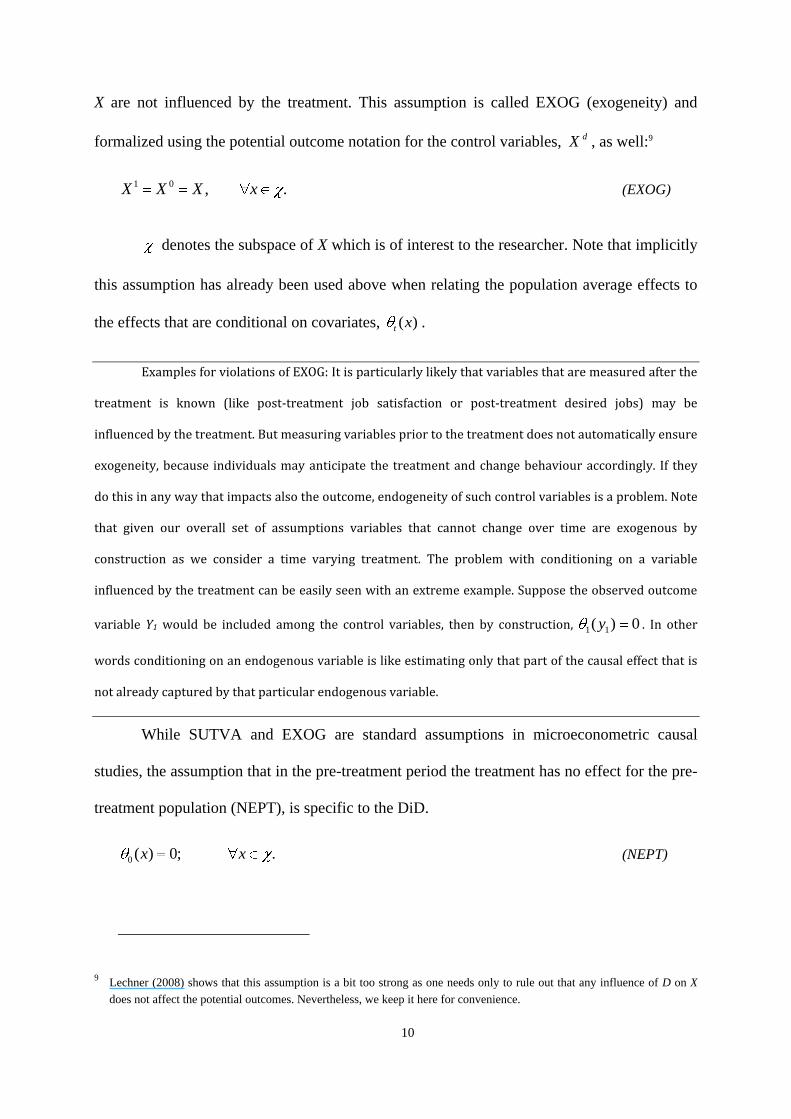
X are not influenced by the treatment. This assumption is called EXOG (exogeneity) and

formalized using the potential outcome notation for the control variables, dX , as well:9

1 0 , .X X X x

(EXOG)

denotes the subspace of X which is of interest to the researcher. Note that implicitly

this assumption has already been used above when relating the population average effects to

the effects that are conditional on covariates, ( )t x .

Examples for violations of EXOG: It is particularly likely that variables that are measured after the

treatment is known (like post-treatment job satisfaction or post-treatment desired jobs) may be

influenced by the treatment. But measuring variables prior to the treatment does not automatically ensure

exogeneity, because individuals may anticipate the treatment and change behaviour accordingly. If they

do this in any way that impacts also the outcome, endogeneity of such control variables is a problem. Note

that given our overall set of assumptions variables that cannot change over time are exogenous by

construction as we consider a time varying treatment. The problem with conditioning on a variable

influenced by the treatment can be easily seen with an extreme example. Suppose the observed outcome

variable Y1 would be included among the control variables, then by construction, 1 1( ) 0y . In other

words conditioning on an endogenous variable is like estimating only that part of the causal effect that is

not already captured by that particular endogenous variable.

While SUTVA and EXOG are standard assumptions in microeconometric causal

studies, the assumption that in the pre-treatment period the treatment has no effect for the pre-

treatment population (NEPT), is specific to the DiD.

0 ( ) 0; .x x (NEPT)

9 Lechner (2008) shows that this assumption is a bit too strong as one needs only to rule out that any influence of D on X

does not affect the potential outcomes. Nevertheless, we keep it here for convenience.

11

NEPT rules out behavioural changes of the treated that influence the outcome in

anticipation of a future treatment.10

Example: This is very similar to the exogeneity condition but now applied to the pre-treatment

outcomes instead of the covariates. For the training example when the outcome of interest is

unemployment, NEPT would be violated if individuals decide not to search for a job because they know

(or plausibly anticipate in a way not captured by X) that they will participate in an attractive training

programme.

Next, we state the defining assumptions for the DiD approach, namely the 'common

trend' (CT) and 'bias stability' (BS) assumptions. The common trend assumption is given by

the following expression:

0 0

1 0

0 0

1 0

0 0

1 0

| , 1 | , 1

| , 0 | , 0 ( )

| | ; .

E Y X x D E Y X x D

E Y X x D E Y X x D CT

E Y X x E Y X x x

This assumption states that the differences of the expected potential nontreatment

outcomes over time conditional on X are unrelated by treatment status. This is the key

assumption of the DiD approach. It implies that if the treated had not been subjected to the

treatment, than both subpopulations defined by D=1 and D=0 would experience the same

time trends conditional on X. Thus, this also implies that the covariates X should be selected

such that they capture all variables that would lead to differential time trends (in other words,

select control variables for which the time trends of the non-participation outcome differ for

10 Note that the observation rule (SUTVA) does not exclude the possibility that the treatment has an effect before it starts

(anticipation), because for the treated we observe their treatment outcome before and after the treatment. Hence, in this

paper we separate SUTVA from the assumption that the treatment has no effect in period zero. Some papers combine

these assumptions by defining the observation rule in a way such that in period zero we always observe the

nonparticipation outcome. In that case, explicitly assuming NEPT is redundant as NEPT is already implied by this type of

observation rule.

12

different values of X, and at the same time for which the distribution of X differs between

treated and controls). The common trend assumption already gives the intuition for the

identification proof. As the nontreatment potential outcomes share the same trend for treated

and nontreated, any deviation of the trend of the observed outcomes of the treated from the

trend of the observed outcomes of the nontreated will be directly attributed to the effect of the

treatment and not to compositional differences of the treatment and control groups.

Example for a violation of the common trend assumption: Suppose that unemployed individuals

from shrinking sectors are particularly likely to be admitted into the training programme. Thus, in the

group of programme participants unemployed who worked in such declining sectors are overrepresented.

As these workers possess sector specific skills, the reemployment chances of unemployed in declining

sectors (sectors that continuously reduce their demand for labour) are likely to deteriorate faster than the

reemployment chances of unemployed searching jobs in sectors that continuously increase their demand

for labour. Since their shares differ in the treated and control groups, the common trend assumption is

violated unconditionally, but may hold if the sector of the last employment is used as a control variable.

As another example, it has been observed by Ashenfelter (1978) that trainees from public training

programmes suffer a larger drop in earnings prior to training than nontrainees. Suppose these drops are

due to negative 'idiosyncratic temporary shocks'. The temporary nature of these shocks implies that

individuals who received the shock will recover faster than other individuals once the effect of the shock

disappears. This directly violates the common trend assumption (see, for example, the exposition of this

problem in Heckman, LaLonde, and Smith, 1999, or in Blundell and Costa Dias, 2009).

An alternative way to see the intuition behind the DiD approach appears when

considering the possibility of estimating the effects of D in both periods while (falsely)

pretending that a selection-on-observables assumption would be correct conditional on X. If

NEPT is true, then a nonzero effect in the estimation of the effects of D on 0Y (in the pre-

treatment period) implies that the estimator is biased and the selection-on-observables

assumption is implausible. If (and only if) this bias is constant over time, it can be used to

13

correct the estimate of the effect of D on 1Y , i.e. in the post-treatment period, which is the

effect we are interested in (e.g., Heckman, Ichimura, Todd, and Smith, 1998). Therefore, the

assumption corresponding to this intuition may be called 'constant bias' assumption (CB) and

is formalized by:

0 0

0 0 0

0 0

1 1 1

| , 1 | , 0 [ ( )]

| , 1 | , 0 [ ( )], .

E Y X x D E Y X x D Bias x

E Y X x D E Y X x D Bias x x (2)

By simple rewriting of the CT and CB assumptions we see that they are identical:

0 0

1 0 1 1

0 0

0 0

0 0

1 0

0 0

1 0

( ) ( ) | , 1 | , 0

| , 1 | , 0

| , 1 | , 1

| , 0 | , 0 .

Bias x Bias x E Y X x D E Y X x D

E Y X x D E Y X x D

E Y X x D E Y X x D

E Y X x D E Y X x D

(3)

From these assumptions it is obvious that identification relies on the counterfactual

difference 0

1 | , 1E Y X x D - 0

0 | , 1E Y X x D being identical to the observable

difference 1 | , 0E Y X x D - 0 | , 0E Y X x D . Therefore, it is necessary that

observations with such characteristics, x, exist in all four subsamples. The assumption that

guarantees this is the so-called common support assumption:

1| , ( , ) ( , ), (1,1) 1; ( , ) (0,1), (0,0), (1,0) ; .P TD X x T D t d t d x (COSU)

Example of a violation of COSU: If participation in a training programme is compulsory for

unemployed below 25, and unemployed below 25 years are subject to a different trend than unemployed

above 25 years (so that this age-cut off is required as conditioning variable to make the common trend

assumption plausible), then the common support assumption would be violated because there would not

be any nonparticipants of age 25 or younger.

14

This assumption is formulated in terms of observable quantities and is thus testable.

All the other (identifying) assumptions mentioned above are formulated in terms of

unobservable random variables and are thus not testable. If common support does not hold for

all values of X, then a common practice would be to redefine the population for which we

estimate the average treatment effects of interest to those treated types, defined by the values

of X ( ), that are observable in all four subpopulations. Alternatively, one may has to be

content with partial identification of the original parameter.11

3.2.2 Proof of identification of the average effect for the treated

Although the proof of identification of the DiD approach is straightforward and

available in the literature, it is instructive and is thus repeated here.

First, note that since the relevant part of X has support in all four subpopulations

defined by the different values of D and T under the common support assumption, once the

conditional-on-X effects, 1( )x , are identified for all relevant values of x, 1ATET is identified

as well (note that 0ATET is zero because of the NEPT assumption). Hence, identification of

1( )x is shown below.

1 0

1 1 1

0

1 1

ìdentified

( ) | , 1

| , 1 | , 1 ;SUTVA

x E Y Y X x D

E Y X x D E Y X x D

0 0 0 0

1 1 0 0

0

1 0 0

identified

| , 1 | , 0 | , 0 | , 1

| , 0 | , 0 | , 1 ;

CT

SUTVA

E Y X x D E Y X x D E Y X x D E Y X x D

E Y X x D E Y X x D E Y X x D

11 See Lechner (2010) for such a strategy in the case of matching that could be directly transferred to the context of DiD

estimation.

15

0 1

0 0

0

ìdentified

| , 1 | , 1

| , 1 .

NEPT

SUTVA

E Y X x D E Y X x D

E Y X x D

Putting all pieces together, we get:

1 1 0

1 0

( ) | , 1 | , 1

| , 0 | , 0 .

x E Y X x D E Y X x D

E Y X x D E Y X x D

Since the value of 1( )x is only a function of random variables for which realisations

are in principle observable, it is identified. Aggregating the conditional effects with respect to

the appropriate distribution of X in the group of the treated in the post-treatment period leads

then to the desired average treatment effect on the treated:

1 | 1 1( )X DATET E x .

The interpretation of the identification of the counterfactual nontreatment outcome is

obvious: We use the pre-treatment outcome of the participants to infer the level of the

nontreatment outcome (by exploiting NEPT) and then infer the change of that potential

outcome that would occur from period zero to period one from the change we actually

observe for the nonparticipants.

Note that the assumptions taken together rule out that the composition of the group of

nontreated is affected by the treatment outcomes (this is mentioned, for example, by Angrist

and Pischke, 2009, as one of the common pitfalls with DiD estimation in practice).

3.2.3 Identification of the average effect for the population and the nontreated

To be able to identify the average effect for the non-treated as well,

1 0 | 0t t tATENT E Y Y D , and thus also to be able to identify the mean effect for the

16

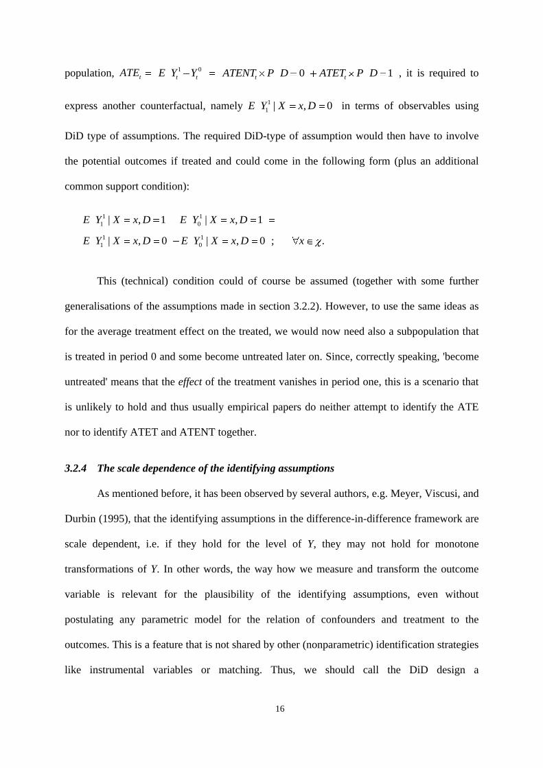
population, tATE 1 0

t tE Y Y 0 1t tATENT P D ATET P D , it is required to

express another counterfactual, namely 1

1 | , 0E Y X x D in terms of observables using

DiD type of assumptions. The required DiD-type of assumption would then have to involve

the potential outcomes if treated and could come in the following form (plus an additional

common support condition):

1 1

1 0

1 1

1 0

| , 1 | , 1

| , 0 | , 0 ; .

E Y X x D E Y X x D

E Y X x D E Y X x D x

This (technical) condition could of course be assumed (together with some further

generalisations of the assumptions made in section 3.2.2). However, to use the same ideas as

for the average treatment effect on the treated, we would now need also a subpopulation that

is treated in period 0 and some become untreated later on. Since, correctly speaking, 'become

untreated' means that the effect of the treatment vanishes in period one, this is a scenario that

is unlikely to hold and thus usually empirical papers do neither attempt to identify the ATE

nor to identify ATET and ATENT together.

3.2.4 The scale dependence of the identifying assumptions

As mentioned before, it has been observed by several authors, e.g. Meyer, Viscusi, and

Durbin (1995), that the identifying assumptions in the difference-in-difference framework are

scale dependent, i.e. if they hold for the level of Y, they may not hold for monotone

transformations of Y. In other words, the way how we measure and transform the outcome

variable is relevant for the plausibility of the identifying assumptions, even without

postulating any parametric model for the relation of confounders and treatment to the

outcomes. This is a feature that is not shared by other (nonparametric) identification strategies

like instrumental variables or matching. Thus, we should call the DiD design a

17

semiparametric identification strategy in contrast to the nonparametric identification

strategies.

This problem can be shown using three examples. Suppose that the potential

nontreatment outcomes are log-normally distributed and that covariates play no role.

Parameterize the log-normal distribution in one of the following ways: (i)

0ln | , ~ (0,2 2 )tY X x D d N d t ; (ii) 0ln | , , ~ ( ,2)tY X x D d T t N d t ; or (iii)

0ln | , , ~ ( , 1)tY X x D d T t N d d , , {0,1}d t . In the first case, the log of the potential

outcome has mean zero and is heteroscedastic. In the second case it is homoscedastic, but its

mean depends on group and time. In the third example we shut down the trends and consider

the stationary case. Consider two choices of scale of Y that are popular for continuous

variables, like earnings for example, namely a log transformation (0lnY ) and the level of the

outcome variable (0Y ). Next, we check whether the CT assumption holds in these settings:12

Case 1: 0ln | ~ (0,2 2 )tY D d N d t

0 0

1 0

0 0

0 0

1 0

0 0

(ln | 1) (ln | 1) 0

(ln | 0) (ln | 0) 0;

E Y D E Y D

E Y D E Y D

2 1

1 0

0 0

1 0

0 0

1 0

1

( | 1) ( | 1) ( 1)

( | 0) ( | 0) 1.

e e

e e

E Y D E Y D e e

E Y D E Y D e

For case I, the common trend assumption holds for the logs, but not for the levels.

Next, we consider case II:

12 Note that

2 2 22 0.5 2ln ~ ( , ) ~ ( , ( 1)( ))Y N Y N e e e .

18

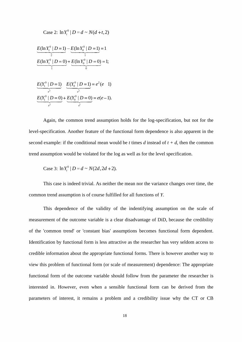
Case 2: 0ln | ~ ( ,2)tY D d N d t

0 0

1 0

2 1

0 0

1 0

1 0

(ln | 1) (ln | 1) 1

(ln | 0) (ln | 0) 1;

E Y D E Y D

E Y D E Y D

3 2

2 1

0 0 2

1 0

0 0

1 0

( | 1) ( | 1) ( 1)

( | 0) ( | 0) ( 1).

e e

e e

E Y D E Y D e e

E Y D E Y D e e

Again, the common trend assumption holds for the log-specification, but not for the

level-specification. Another feature of the functional form dependence is also apparent in the

second example: if the conditional mean would be t times d instead of t + d, then the common

trend assumption would be violated for the log as well as for the level specification.

Case 3: 0ln | ~ (2 ,2 2).tY D d N d d

This case is indeed trivial. As neither the mean nor the variance changes over time, the

common trend assumption is of course fulfilled for all functions of Y.

This dependence of the validity of the indentifying assumption on the scale of

measurement of the outcome variable is a clear disadvantage of DiD, because the credibility

of the 'common trend' or 'constant bias' assumptions becomes functional form dependent.

Identification by functional form is less attractive as the researcher has very seldom access to

credible information about the appropriate functional forms. There is however another way to

view this problem of functional form (or scale of measurement) dependence: The appropriate

functional form of the outcome variable should follow from the parameter the researcher is

interested in. However, even when a sensible functional form can be derived from the

parameters of interest, it remains a problem and a credibility issue why the CT or CB

19

assumptions should be plausible for that particular choice of function, while they may be

violated for other choices, which might be common choices as well.

3.2.5 The changes-in-changes model by Athey and Imbens (2006)

The functional form dependence is the starting point for the so-called 'changes-in-

changes model' that has been proposed by Athey and Imbens (2006). The goal of their paper

is state a set of DiD-like assumptions that are not scale dependent.

The CiC ('Changes-in-Changes') model proposed by Athey and Imbens (2006) is

based on the same idea for the distribution of the potential outcomes than the DiD model is

for expectations. The change of the distribution of the nontreatment outcome of the nontreated

over time is used to infer how the distribution of the nontreatment outcomes of the treatment

group would have changed had they not experienced the treatment. The key difference is that

the assumptions made, and the information exploited for identification and estimation comes

from all of the distribution and not just from the first moments as in DiD estimation.

Estimation is based on estimating cumulative distribution functions as well as their inverses

for each of the three groups defined by treatment and time conditional on X and predicting the

counterfactual outcomes based on those functionals.

Although the estimation problem is straightforward in principle (the authors provide

N consistent and asymptotically normal estimators), considerable problems may appear in

practice either if the outcome variables are not continuous or the types of individuals is too

heterogeneous (based on the different relevant values of x). In the first case, the problem is

that the inversion of a cumulative distribution function of a discrete random variable is not

unique. Therefore, only bounds of the true effects are identified. In the second case, when

control variables are present, estimation either has to be performed within cells defined by the

discrete values of those variables, or appropriate smoothing techniques have to be used in the

20

case of continuous variables (or discrete variables with many different possible values). Both

issues are only of limited concern asymptotically. However, given the usual dimensions of the

control variables and sample sizes in applications, this type of curse of dimensionality could

be a major concern for applied researchers who may need to control for many variables to

make the common trend assumption sufficiently credible. Perhaps for this reason the number

of empirical applications of this approach so far is rather limited. The only application known

to the author (other than the one provided by Athey and Imbens in their seminal paper) is the

one by Haves and Mogstad (2010) who analyse the effects of child care in Norway. They are

interested not only in mean impacts but they are also interested in the effects on the quantiles

of the earnings distribution.

3.2.6 The role of covariates

As mentioned above, we need to control for exactly those exogenous variables that

lead to differential trends and are not influenced by the treatment. Including further control

variables (assuming that the common trend assumption still holds conditional on this extended

set of covariates) has positive and negative aspects. On the positive side, it could help to

detect effect heterogeneity that may be of substantive interest to the researcher (e.g.

estimating the effects for men and women separately although men and women experience the

same trends for their potential outcomes). On the negative side, every additional variable

makes the common support assumption more difficult to fulfil.

So far we discussed the case of time constant covariates. In many studies, though,

measurements in different time periods may be available. In particular in a repeated cross-

section setting, it is likely that the only measurement of some covariates available happens at

the same time as for the outcome variables. The particular concern here is the post-treatment

period, because time varying trend confounding variables measured after the treatment are

more likely to be influenced by it. Thus, the exogeneity condition would be violated. In this

21

case, controlling for such time varying covariates may lead to biased estimates. Generally,

time varying covariates are no problem or may even be better suited to remove trend

confounding if they are exogenous (for example using age instead of birth year may be a

superior choice to remove trend confounding in some applications). If these variables are not

exogenous and if anticipation effects play no role for them, then using pre-treatment

measurements whenever available may be the best empirical strategy.

Now, we change the perspective somewhat and look at the type of circumstances

under which an unobservable variable that influences the potential outcomes can be safely

ignored when estimating a DiD model. To see this, we consider the impact of the excluded

(perhaps unobservable) time constant variable U on this estimation strategy in the simplest

case without covariates. Obviously, we need to require CT to hold unconditionally, because U

is unobserved. To see its role on the unconditional common trend assumption, we use iterated

expectations:

0 0

| 1 1 0

0 0

| 0 1 0

: | 1, | 1,

| 0, | 0, .

U D

U D

CT E E Y D U u E Y D U u

E E Y D U u E Y D U u (4)

Clearly, if the common trends assumption holds conditional on U (if not, then there is

no reason to consider using U as an additional control anyway) and if the distribution of U

does not depend on the treatment group, then U can be safely ignored in the estimation

without violating CT.

Next, consider again the case that CT holds conditional on U, but that the distribution

of U differs with different values of D as well. In this case, if U cannot be used as covariate,

further assumptions are required. One such assumption is that the effect of the unobservable

variable on the potential outcomes is constant over time (but may vary across treatment

groups). The following separable structure has such a property:

22

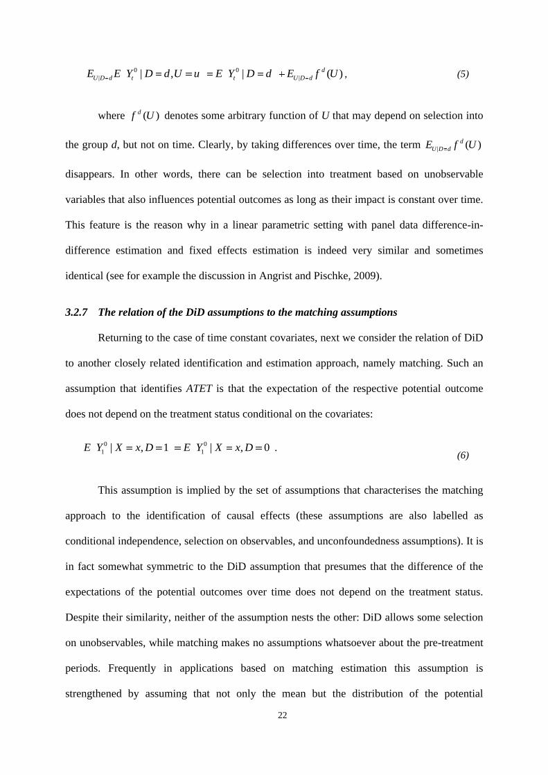
0 0

| || , | ( )d

U D d t t U D dE E Y D d U u E Y D d E f U , (5)

where ( )df U denotes some arbitrary function of U that may depend on selection into

the group d, but not on time. Clearly, by taking differences over time, the term | ( )d

U D dE f U

disappears. In other words, there can be selection into treatment based on unobservable

variables that also influences potential outcomes as long as their impact is constant over time.

This feature is the reason why in a linear parametric setting with panel data difference-in-

difference estimation and fixed effects estimation is indeed very similar and sometimes

identical (see for example the discussion in Angrist and Pischke, 2009).

3.2.7 The relation of the DiD assumptions to the matching assumptions

Returning to the case of time constant covariates, next we consider the relation of DiD

to another closely related identification and estimation approach, namely matching. Such an

assumption that identifies ATET is that the expectation of the respective potential outcome

does not depend on the treatment status conditional on the covariates:

0 0

1 1| , 1 | , 0 .E Y X x D E Y X x D (6)

This assumption is implied by the set of assumptions that characterises the matching

approach to the identification of causal effects (these assumptions are also labelled as

conditional independence, selection on observables, and unconfoundedness assumptions). It is

in fact somewhat symmetric to the DiD assumption that presumes that the difference of the

expectations of the potential outcomes over time does not depend on the treatment status.

Despite their similarity, neither of the assumption nests the other: DiD allows some selection

on unobservables, while matching makes no assumptions whatsoever about the pre-treatment

periods. Frequently in applications based on matching estimation this assumption is

strengthened by assuming that not only the mean but the distribution of the potential

23

outcomes conditional on covariates is independent of the treatment status. This assumption

has the virtue that it identifies not only the counterfactual expectations, but the full

counterfactual distribution. Furthermore, it makes the identification invariant to the chosen

scaling of Y. Although the same approach can be chosen in a difference in difference

framework, namely assuming that the difference of the potential outcomes over time are

independent of the treatment, Appendix A.2 shows that there are no such gains for DiD

estimation as there are for matching. Hence, the 'independence of the differences of the

potential outcomes over time' assumption is not so attractive, because compared to the

common trend in means assumption it is more restrictive without identifying further

interesting quantities.

3.2.8 Panel data

So far, this exposition was silent on whether the same individuals are observed in the

pre- and post-treatment periods, because all identification results valid for repeated cross-

sections also hold for panel data. So even though with panel data individual pre-treatment-

post-treatment differences of outcome variables can be directly formed, the nature of the

estimator is still the same, although its precision may change.

One consequence of basing the estimator on individual differences over time is that all

influences of time constant confounding factors that are additive separable from the remaining

part of the conditional expectations of the potential outcomes are removed by the DiD

differencing as shown in the previous section. Therefore, it is not surprising that in the

regression formulation below, adding fixed individual effects instead of the treatment group

dummy d (and all time constant covariates X), will lead to the same estimand (e.g. Angrist and

Pischke, 2009).

Furthermore, from the point of view of identification, a substantial advantage of panel

data is that matching estimation based on conditioning on pre-treatment outcomes is feasible

24

as well. This is important because it appears to be a natural requirement for a 'good'

comparison group to have similar pre-treatment means of the outcome variables. This is not

possible with repeated cross-sections since we do not observe pre-treatment outcomes from

the same individuals, but only from some group that is similar to the individuals obtaining the

treatment in terms of other observable characteristics X.

The corresponding matching-type assumption when lagged outcome variables are

available can be expressed as follows:

0 0

1 0 0 1 0 0| , , 1 | , , 0 .E Y Y y X x D E Y Y y X x D (7)

Imbens and Wooldridge (2009) observe that the common trend assumption and this

matching-type assumption impose different identifying restrictions on the data which are not

nested and must be rationalized based on substantive knowledge about the selection process,

i.e. only one of them can be true. Angrist and Krueger (1999) elaborate on this issue on the

basis of regression models and come to the same conclusions. The advantage of the DiD

method is that it allows for time constant confounding unobservables while requiring common

trends, whereas matching does not require common trends but assumes that conditional on

pre-treatment outcomes confounding unobservables are irrelevant. Of course, one may argue

that conditioning on the past outcome variables already controls for that part of the

unobservables that manifested themselves in the lagged outcome variables.

One may try to combine the good features from both methods by including pre-

treatment outcomes among the covariates in a DiD framework. This is however identical to

matching: Taken the difference while keeping the pre-treatment part of that difference

constant at the individual level in any comparison (i.e. the treated and matched control

observations have the same pre-treatment level) is equivalent to just ignoring the difference in

DiD and focus on the post-treatment variables alone. Thus, such a procedure implicitly

25

requires the matching assumptions.13 In other words, assuming common trends conditional on

the start of the trend (which means it has to be the same for treated and controls) is basically

identical to assume no confounding (i.e. the matching assumptions hold) conditional on past

outcomes.

Thus, Imbens and Wooldridge's (2009, p. 70) conclusion about the usefulness of DiD

in panel data compared to matching is negative: "As a practical matter, the DID approach

appears less attractive than the unconfoundedness-based approach in the context of panel data.

It is difficult to see how making treated and control units comparable on lagged outcomes will

make the causal interpretation of their difference less credible, as suggested by the DID

assumptions." However, a recent paper by Chabé-Ferret (2010) gives several examples in

which a difference-in-difference strategy leads to a consistent estimator while matching

conditional on past outcomes may be biased. He also shows calibrations based on real data

suggesting that this bias may not be small.

3.2.9 The regression formulation

Derivation of the linear specification

Most of the empirical applications conducted so far employing the DiD identification

strategy use the linear model. The linear regression formulation can be motivated by the

following assumptions about the conditional expectations for the potential outcomes:

1 1 1

0 0 0

| , ;

| , ; 0,1 , .

t

t

E Y X x D d t d x tx dx

E Y X x D d t d x tx dx d x (8)

13 Although the confounding individual effect has been removed by taking differences, conditioning on the pre-treatment

levels is like conditioning on it again and thus may induce a correlation with D. In other words, if the DiD assumptions

hold unconditionally on the pre-treatment outcome, they are likely to be violated conditional on pre-treatment outcomes.

26

The specification is flexible to some degree as it includes several interaction terms

between the control variables and group membership. However, it does not include

interactions between time and treatment status as these interactions would violate the common

trend assumption.14 Note that some of the coefficients do not vary across potential outcomes

as a simple way to ensure that the treatment has no effect in period zero.15

Next, note that this specification indeed fulfils the common trend assumption:

0 0

1 0

0 0 0 0

| , 1 | , 1

;

E Y X x D E Y X x D

x x x x x x

0 0 0 0

1 0 1 1

0 0

1 1

| , 0 | , 0

.

E Y X x D E Y X x D x x x

x

These derivations make it again clear that having differential trends for the different

potential outcomes is no problem as long as the trends do not depend on the treatment status.

Starting from the specifications for the potential outcomes, the effects can be

expressed in terms of their regression coefficients:

14 This exclusion restriction gives rise to an interpretation of difference-in-difference estimation as conditional (on X, D, and

T) IV estimation with the interaction term D T acting as an instrument (with perfect compliance). This interpretation again

points to the essentially parametric nature of this approach, as there cannot be independent variation of this instrument

given its components D and T. This is only possible when a (semi-) parametric model is specified in which the effects of

D1 and T are separable.

15 In a more general model, we would have | , andd d d d d d d

tE Y X x D d t d x tx dx

!1 0 1 0 1 0 1 0 1 0

0 0 | , ( ) ( ) [( ) ( )] 0.E Y Y X x D d d x d

27

1 1 0 0

1 1 0

1 0

1 1 0

1 0 1 0

( ) | , 1 | , 1

| , 0 | , 0

( ) ( ) [( ) ( )]

( ) ( ) .

x x

x E Y X x D E Y X x D

E Y X x D E Y X x D

x x x x x x x x

x x

Therefore, the task of regression estimation is to obtain consistent estimates of and

. To do so, we derive the regression model for the observed outcome variable.

The observation rule (SUTVA), 1 0(1 )t t tY dY d Y , leads to the following

specification for the observed outcome:

1 0

1 0

1 1 0 0

0 0 1 1 0 0

0 0 1 0

| , (1 ) | ,

| , (1 ) | ,

( ) (1 )( )

( )

( )

t t t

t t

E Y X x D d E dY d Y X x D d

dE Y X x D d d E Y X x D d

d t x tx x d t x tx

t x tx d t x tx x t x tx

t x tx d x t t1 0

0 0

( )

; 0,1 , .

x

t d x tx dx dt dtx d x

From these derivations, we see that a regression with group and time dummies (so-

called main effects) plus the various interaction terms identify the causal effects. In such a

regression, the coefficients of the interaction terms between time and treatment group capture

the effects. It is rather common practice to assume that the coefficient is zero, implying

that the interaction of group and time with the control variables disappears.

Advantages of the regression formulation

The clear advantage of the regression formulation of the DiD identification and

estimation problem is the easiness of obtaining the final estimates and their standard errors

(although even in this simple case there are some DiD specific problems discovered recently

28

that will be discussed below). Furthermore, we can easily extend the model to cover more

periods and more treatments, including continuous treatments, and add additional covariates

without further relevant computational burden.

Disadvantages of the regression formulation

However, there are also disadvantages of this approach concerning (i) the effect

heterogeneity that is allowed for, (ii) the way how control variables are included, and (iii) the

possibility of arriving at estimates that are not plausible. It is important to note that those

issues only appear if covariates are included (and required to make the common trend

assumption plausible). If covariates are not required, then estimation of the effects in DiD

designs using the linear regression framework described above is fully nonparametric (in the

sense that it does not impose any further assumptions than the ones needed for identification,

which were discussed in the previous section).

Let us consider the potential issues (restrictions implied by the regression framework)

in turn. First, for the issue of effect heterogeneity consider the simpler case in which equals

0. If there is indeed any effect heterogeneity, it means that the true coefficient is random

instead of being a constant. Since the regression estimation assumes a nonstochastic

coefficient, the stochastic deviation that cannot be captured in the regression becomes part of

the error term. This may not be harmful, if the heterogeneity is pure random noise

uncorrelated with all variables included in the regression or if the model is fully saturated in

the controls variables (see Angrist and Pischke, 2009). The regression coefficient still

captures the average effect. However, if the heterogeneity is related to those variables and the

model is not fully saturated in the covariates, then for example estimated by OLS is

inconsistent (and asymptotically biased) for the ATET.

29

Second, including the control variables in a linear fashion implies the assumption of

common trends conditional on the linear index, X , which is more restrictive than assuming

common trends conditional on X. Any deviation from the linear index is again absorbed in the

regression error term and may invalidate the estimates.

Finally, if the outcomes have limited support, such as a binary variable, there is no

guarantee that the predicted expected potential outcomes will respect this support condition.

The latter is one of the reasons why in practice linear models are rarely used in these cases

and nonlinear models, like logits or probits in the case of a binary variable, are preferred.

However, they come with their particular problems in a DiD setup.

Nonlinear models with the standard common trend assumption

There are many types of outcome variables for which it is common practice to use

nonlinear models instead of linear ones, because they provide a better approximation of the

statistical properties of such random variables. Popular examples are probit, logit, Tobit,

count data models, and duration models. The general arguments in favour of such models do

not however carry over to effects identified by the DiD assumptions. When applying

nonlinear models in such a framework, researchers typically use a linear index structure

together with a nonlinear link function (e.g. Hunt, 1995, Gruber and Poterba, 1994). The

linear index structure is specified as it would be a specification for the linear regression

model. Then, the model is estimated and the estimated coefficients or (average) marginal

effects are interpreted causally. However, while the linear regression can be derived from the

DiD assumptions together with some restrictions on functional forms, such rationalisation is

generally impossible for nonlinear models. To see this more clearly, let us consider a

nonlinear regression model in the same fashion as we analysed the corresponding linear

model.

30

We start with a 'natural' nonlinear model with a linear index structure which is

transformed by a link function, ( )G , to yield the conditional expectation of the potential

outcome. In the case of the probit this link function would for example be the cumulative

distribution function of the standard normal distribution:

1 1 1

0 0 0

| , ( );

| , ( ); 0,1 , .

t

t

E Y X x D d G t d x tx dx

E Y X x D d G t d x tx dx d x (9)

This specification resembles the linear model with the exception of the addition of the

link function. It fulfils the NEPT assumption. Using the observation rule and performing the

same transformation as for the linear model (inside the ( )G -function), we obtain the

following specification for the observable outcomes that can be used for the econometric

estimation of the model parameters (again, using the notation as introduced for the linear

model above):

1 0

1 0

1 1 0 0

0 0

| , (1 ) | ,

| , (1 ) | ,

( ) (1 )( )

...

; {0,1}, .

t t t

t t

E Y X x D d EdY d Y X x D d

dE Y X x D d d E Y X x D d

G d t x tx x d t x tx

G t d x tx dx dt dtx d x

(10)

This equation, sometimes with fewer interaction terms, is the basis for the empirical

analysis of the papers using (standard) nonlinear difference-in-differences.16

Of course, as for the linear model, we need to check whether such a specification

indeed fulfils the common trend assumption:

16 On different ways to estimate 'causal' parameters from these models, see the papers by Ai and Norton (2003) and Puhani

(2008).

31

1 0

1 0

| , 1 | , 1

( ( )) ( ( ));

| , 0 | , 0

( ( )) ( ); 0,1 .

d d

d d

d d

d d

E Y X x D E Y X x D

G x G x

E Y X x D E Y X x D

G x G x d

It may or may not come as a surprise, but the intuitive specification does not fulfil the

common trend assumption, as this assumption relies on differencing out specific terms, which

does not happen in a nonlinear model. Indeed, the common trend assumption would only be

respected if and would be zero. However, these are exactly those coefficients that

capture the group specific differences. This is to say that whereas the linear specification

required the group specific differences to be time constant, the nonlinear specification

requires them to be absent which removes the attractive feature of the difference-in-difference

approach that it allows for some selection on group and individual specific differences. Thus,

we conclude that estimating a difference-in-difference model with the standard specification

would usually lead to an inconsistent estimator if the standard common trend assumption is

upheld.

In other words, if the standard DiD assumptions hold, this nonlinear model does not

exploit them (it will usually violate them), and thus estimation based on this model does not

identify the causal effect of D on Y. Let us generalize the above model by using group specific

coefficients.

1 1, 1,

0 0, 0,

| , ( );

| , ( ); 0,1 .

d d d d

t

d d d d

t

E Y X x D d G t x tx

E Y X x D d G t x tx d (11)

Note that the terms dd and ddx are absorbed by the group specific constant and

slope ( d and dx ). For the common trend assumption, we then obtain:

32

1 0

1 ,1 1 ,1 1 1

1 0

0 ,0 0 ,0 0 0

| , 1 | , 1

( ) ( );

| , 0 | , 0

( ) ( ); {0,1}.

d d

d d

d d

d d

E Y X x D E Y X x D

G x G x

E Y X x D E Y X x D

G x G x d

This model fulfils the common trend assumption under a set of restrictions on the

coefficients (e.g., 1 ,1 0 ,0d d

, 1 0 1 ,1 0 ,0d d , 1 0 , so that

,1 ,0d d d and ,1 ,0d d d

). However, those restrictions imply, as before, that there

are no group effects and thus this parameterization for the potential outcomes is not attractive

either. Thus, 'standard' nonlinear parametric specifications of the potential outcomes and the

derived observed outcomes are not attractive as they fulfil the DiD assumptions only under

additional constraints.17

Since the simple way of using standard parametric models does not work in the

nonlinear case when identification is achieved by the difference-in-difference assumptions,

what are the alternatives? One alternative is to use a linear specification despite its

problematic features for outcome variables with bounded support, for example. A second

alternative is to use nonlinear parametric approximations to predict the four components of

the conditional-on-X effects, | ,tE Y X x D d , , 0,1t d in a parsimonious way, and

then average those conditional-on-X effects according to the desired distribution of

confounders to obtain estimates for the treated population. For example, with a binary

17 This phenomena has already been observed by Meyer (1995, p. 155), who explains it in the following way: "… if the

mean of the outcome variable is very different in the treatment and control group, then [comparing expectations of means

in the four groups] could not be an appropriate model both in levels and in means … This problem occurs because

nonlinear transformations of the dependent variable imply different marginal effects on the dependent variable at different

levels of the dependent variable. Thus time could not have an effect of the exact same magnitude in both treatment and

control groups in both a linear and a logarithmic specification." A similar observation has been made by Heckman (1996)

in his discussion of a paper by Eissa (1996).

33

outcome variable we may want to estimate a probit model in all three subsamples and obtain

the following estimator for the average treatment effect on the treated:

0 1 0

1 1 1 0 0

1

ˆ ˆ ˆ( ) ( ) ( )N

i i i i i i

i

ATET d t y x x x , (12)

where ˆ d

t denotes a vector of coefficients (including a constant) estimated by a probit

with dependent variable, tY , in the subsample defined by group d in period t. ( )a denotes

the cumulative distribution function of the standard normal distribution evaluated at a. Note

that one may also predict the outcome for the treated in the post-treatment periods, but the

average of such a prediction should be close to the mean of the outcome (it would be identical

if a logit model is used).

Estimating three probit models is of course similar to estimating a model in the overall

sample (or the three subsamples) which is fully interacted with respect to t and d. In practice

one may wish to estimate a more parsimonious specification by omitting some of those

interaction terms.

Although this approach may work well in practice (however, I am not aware of any

applied literature using such a specification in this way), a drawback of using these

approximations is that we cannot recover the exact functional specifications of the mean

potential outcomes, which makes it harder to understand the underlying restrictions that come

from the required functional form assumptions.

Nonlinear models with a modified common trend assumption

In the previous section, we showed that commonly used nonlinear models violate the

common trend assumption. Here, we show that indeed for certain types of outcome variables

the nature of these outcome variables makes it hard to believe from the outset that common

trends may prevail. To give an example, assume that a binary variable for a particular group

34

of nontreated in the post treatment period has mean 0.9. The gap between the treated and

nontreated groups prior to treatment was 0.2 in favour of the treated. In this case, adjusting for

common trends would lead to an expected nontreatment outcome of 1.1, which would be

outside the support of the outcome variable. Thus, in this example the common trend

assumption must be violated.18

Following ideas similar to those of Blundell et al. (2009), we now explore the potential

of a different way to specify identifying assumptions that resemble the key ideas of

difference-in-difference estimation, but may appear to be more plausible than the common

trend assumption for variables with bounded support and other cases in which the original

DiD assumption appears implausible.19 The following exposition is based on the concept of a

latent variable that figures very prominently in microeconometrics to link standard

econometric linear models to discrete, censored or truncated dependent variables.

Concretely, assume that the conditional expectation of the observable outcome

variable, Y, is related to the conditional expectation of a latent outcome variable, Y*, in the

following way:

0 0*

1| , ( | , ) ; , {0,1}, .t tE Y X x D d H E Y X x D d d t x (13)

The function ( )H is assumed to be strictly monotonously increasing and invertible (

1( )H ). Therefore, we get:

0* 1 0| , ( | , ) ; , {0,1}, .t tE Y X x D d H E Y X x D d d t x

18 I thank Patrick Puhani for a most interesting discussion on this subject.

19 Blundell et al. (2009) use specifications based on various error terms that lead to the same results as the more direct

approach followed here.

35

The function ( )H plays the role of the typical link functions that appear for example

in models like the probit, logit, Tobit, and other models. In the probit model ( )H would be

the cumulative distribution function of the standard normal distribution. Now let us assume

common trends at the level of the expectations of the latent outcome variables:

0* 0*

1 0

0* 0*

1 0

0* 0*

1 0

| , 1 | , 1

| , 0 | , 0 ( *)

| | , .

E Y X x D E Y X x D

E Y X x D E Y X x D CT

E Y X x E Y X x x

Clearly, whether this assumption is plausible or not depends on the particular

parameterisation of the model which critically involves the ( )H function. Even more

important is that at least in some cases a substantive meaning can be given to the latent

outcome variable, like a utility or an earnings potential, for example, which can then be used

as the basis for judging the credibility of this assumption.

Using (NEPT) and the modified common trend assumption, we can show that the

usual effects are identified:

1 0 1 0 1 01 1 0

1 00

11

0* 0* 0*

1 1 0

| , 1 | , 0 | , 0

0*

0

| , 1

1 0

1

| ,

| , 1 | , 0 | , 0

| , 1

| , 0

H E Y X x D H E Y X x D H E Y X x D

H E Y X x D

H E Y X x D

E Y X x D E Y X x D E Y X x D

E Y X x D

H E Y X x D

10

10

1 0

0

0 | , 0

1 0

0

| , 1

1 1

1 0

1

0

| , 0

| , 1

| , 0 | , 0

| , 1 .

H E Y X x D

H E Y X x D

H E Y X x D

H E Y X x D

H E Y X x D H E Y X x D

H E Y X x D

Therefore, we can express the missing counterfactual 0

1 | , 1E Y X x D as

36

0 *0

1 1

1

1

1 1

0 0

| , 1 | , 1

| , 0

| , 0 | , 1 .

E Y X x D H E Y X x D

H H E Y X x D

H E Y X x D H E Y X x D

Thus, ATET1 is identified.20

As an example consider a binary outcome variable analysed with a probit model in its

linear index form with subsample specific coefficients. In this case ( )H will be the

cumulative distribution function of the standard normal distribution, , and 1H will

be the respective inverse, 1 , which exists and is unique in this case. Such a probit model

is defined as:

| , ( ).d

t tE Y X x D d x (14)

This expressions leads to the final result:

0 1 0 1 0 1 1

1 1 0 0

0 0 1

1 0 0

| , 1 ( ) ( ) ( )

( ).

E Y X x D x x x

x x x

Letting 0

1̂, 0

0ˆ , and 1

0ˆ be consistent estimates of the unknown coefficients leads to

the following expression for the missing mean potential outcome and thus average treatment

effect on the treated can be consistently estimated by:

0 0 1 1

1 1 1 0 011 1

1ˆ ˆ ˆ( ) , .

N N

i i i i i

i i

ATET d t y x x x N d tN

It is obvious that this expression is different from the one given above that was also

based on the probit model. Although both examples are based on a probit model, the former

20 Note that when leaving out the covariates, this is exactly the expression derived by Blundell et al. (2009, page 586).

37

assumes common trends for the expected potential outcomes, whereas the latter assumes

common trends for a nonlinear transformation of the expected outcomes. As already seen

before, DiD is functional form dependent, hence such transformations matter and lead to

different results.

4. Some issues concerning estimation

4.1 Parametric models

So far, most empirical studies relying on a difference-in-difference approach are using

parametric models. In this case, estimation is usually simple, at least as long as the model that

is required to be estimated is either a linear or a standard nonlinear model. Of course, if the

model is based on a DiD assumption imposed on some complex transformation as discussed

in the previous section on nonlinear models, it may be that even estimating a parametric

model may be demanding and subject to substantial problems (like excessive computation

time, convergence problems, or nonunique objective function, etc.). However, there is a large

literature in microeconometrics about these issues and their possible solutions. The fact that

there is a type of DiD assumption involved does not create additional problems. Even in the

parametric case there may be DiD-specific problems with inference from the standard

estimators that will, however, be addressed in the section about inference below.

4.2 Semiparametric and nonparametric models

When no covariates are present estimation can be still be based on the regression

formulation without being restrictive in any sense. Thus, standard linear estimators, like OLS,

can be used and will have desirable properties. OLS based on a constant, the group and time

dummies as well as their interaction is identical to the typical DiD comparison of the four

sample means. When covariates are included and the chosen specification is not rich enough

38

to lead to a saturated model (usually because the number of observations is too small within

each cell to allow for a complete set of interactions), the consistency of OLS is not guaranteed

and may depend on the validity of the functional form assumptions. Generally, regression is

restrictive because it depends on a linear index function to capture the influence of covariates

on the outcomes and it restricts effect heterogeneity (see the in-depth discussion of the

properties of linear estimation in such settings by Angrist and Pischke, 2009). Whether the

resulting bias is a serious one or only a small one is usually impossible to judge in an

application.

The issue of allowing covariates to enter the estimator in a very flexible way can

however be tackled similarly to the approaches taken by the semiparametric matching

literature. To see this, start by rewriting the average treatment effect on the treated in the

following way:

1

1

1 | 1 1

1 | 1 1

| 1 0

| 1 0

( )

| 1 | , 0

| , 1

| , 0 .

X D

X D

X D

X D

ATET E x

E Y D E E Y X x D

E E Y X x D

E E Y X x D (15)

The first observation is that in order to estimate 1ATET consistently a consistent

estimate of the conditional on X effect, 1( )x , is not necessary. Any estimate that will

consistently estimate 1ATET will have to reweight the outcomes observed in the three

'counterfactual' sup-populations (defined by T and D) such that these weights applied to the

covariates will make the covariate distribution in the particular subpopulation identical to the

one observed in the target population (T = 1, D = 1).

The second observation is that the structure of the estimand is very similar to the one

for matching estimation for which a large literature exists (see for example the survey by

39

Imbens, 2004). The difference is that instead of adjusting a covariate distribution in just the

one subsample of nontreated, within a 2-period DiD framework three covariate distributions

have to be adjusted because there are three nontreated groups. In other words, the

combination of three consistent matching estimators in the respective subsamples will lead to

a consistent estimator of the population effects (if there additional time periods are available,

the number of matching estimations increases by two for every additional period). It is also

worth noting that the so-called propensity score properties first shown by Rosenbaum and

Rubin (1983) for the case of matching can be applied here as well:

| 1

( , , )| 1

| ,

| ( , , ) ( , , ), ;

( , , ) : ( 1| , ( , ) {( , ), (1,1)}].

X D t

p X t d D t

E E Y X x D d

E E Y p X t d p x t d D d

p X t d P TD X x T D t d (16)

The common support assumption (COSU) ensures that these probabilities, called

propensity scores in the matching literature, are positive. This general property is in principle

already contained in the results derived by Rosenbaum and Rubin (1983). The proof for the

DiD case is sketched in Appendix A.1.

So far studies using semiparametric or nonparametric covariate adjustments in DiD

estimation are rare. The first paper to observe that DiD estimators can be based on matching

seems to be Heckman, Ichimura, and Todd (1997). They base their estimators on local linear

kernel estimators, as do Bergemann, Fitzenberger, and Speckesser (2009).

Acemoglu and Angrist (2001), whose empirical analysis is based on a very large

sample and a fairly small number of discrete covariates, compute the respective means within

the cells defined by the covariates and then weight the resulting differences with the

probability of the particular cell in the population.

40

Eichler and Lechner (2002) use simple propensity score matching methods, while

Blundell, Meghir, Costa Dias, and van Reenen (2004) use a time specific and cross-section

specific propensity score in their matching methods (see also Blundell and Costa Dias, 2009).

Ravallion, Galasso, Lazo, and Philipp (2005) use propensity score matching as well to purge

their estimates of differences coming from different distributions of trend confounders in the

various subsamples.

Abadie (2005) proposes estimators based on weighting the outcomes by the propensity

scores combined with linear projections. He also provides distribution theory for the case of

using a nonparametric estimator for the propensity score. Finally, in an empirical application

Bühler, Helm, and Lechner (2010) also use weighting on the propensity score. They propose

to estimate different scores for each of the 3 comparisons involved.

5. Some DID-specific issues about inference

Recently, there has been a renewed discussion about how to conduct inference in a

(usually parametric) DiD setting. These papers are concerned with potential correlations over

time as well as within groups (in particular with panel data). Note that if we have

period/group-specific randomness (e.g. group-time-specific individual random effects),21 then

with a finite number of periods and groups, no consistent estimator can exist, because within

group averaging cannot eliminate such variability. The only way to reduce this type of

uncertainty is to have more periods and more (nontreatment) groups. The issue of correlations

over time of the units in the different groups (like states before and after a policy change) as

well as their cross-sectional correlation within groups has been analysed within a regression

21 Of course, (additive separable) treatment group specific uncertainty that is constant over time, as well as time specific

uncertainty that is constant over groups, is differenced out by taking the differences of the four group means.

41

framework by Bertrand, Duflo, and Mullainathan (2004), Donald and Lang (2007), Hansen

(2007a, 2007b) allowing for multiple time periods and groups. These papers conclude that

inference may be substantially affected by such cluster effects (see also the informative

discussion about these issues within a regression-type framework in Imbens and Wooldridge,

2009, p. 69). Conley and Taber (2005) approach this problem somewhat differently. They

consider the case of a small number of treated and an expanding number of controls and

develop distribution theory under this scenario that is likely to appear in many applications.

Although even in this case DiD estimators will generally be inconsistent, at least their

asymptotic distribution can be used to perform standard tests.

6. Further issues

6.1 Very small number of treated and control units / interventions at the aggregate

level

There may be a problem for identification, estimation and inference if, for example,

one region is subject to a treatment in period t (i.e. all units are subject to the new regime),

whereas a couple of other regions are not subject to it. First, note that this may create some

problem for identification, if the other regions have different time trends of the potential

outcomes compared to the treatment region. Abadie, Diamond, and Hainmüller (2007)

suggest treating this problem essentially as a matching problem. They propose using a

weighted average of all the control regions with weights chosen such that the weighted mean

of the covariates in the control regions are equal, or at least as similar as possible, to the

observed values in the treatment region after the treatment. Furthermore, the authors also

argue that even in such aggregate studies, one should account for uncertainty (one may argue

that one observes the population and, thus, there is no need to take sampling uncertainty into

account) and provide some inference procedures that (i) do not rely on asymptotic theory and

42

are valid in small samples, and (ii) take account of other uncertainty than sampling

uncertainty.22

6.2 Additional periods

For most of the paper the simplest case of just two periods has been considered. This

is enough to achieve identification of the usual quantities of interest. Now, we consider the

value added by having more (post- and / or pre-treatment) periods of data available. It is

assumed that in all pre-treatment periods, the (future) treatment group is identified and that for

all pre- and post-treatment periods the same covariates (that are not influenced by the future

or past treatment) are observed.

Before however expanding on the advantages of having more post- and pre-treatment

periods, it has to be mentioned that they are only useful if the common trend assumptions

holds for all pre- and post-treatment comparisons. This may become particularly implausible

or plausible if the periods are further away from each other depending on the particular

scenario. Although derived in a fairly restrictive framework, the paper by Chabé-Ferret (2010)

points to cases when for example an estimator using pre-post-treatment pairs with equal time

distance to the treatment is consistent while using just the most recent pre-treatment period

leads to an inconsistent estimator. Unfortunately, he also shows examples in which the

opposite is true. Apparently, more research is required on this important topic.

6.2.1 Dynamics of the effects

Suppose we have additional post-treatment knowledge. If the common trend

assumptions are valid for all comparisons with the pre-treatment period, then the additional

22 The already mentioned paper by Donald and Lang (2007) is also particularly interested in the case of a small number of

treated and controls, while the study by Conley and Taber (2009) mentioned above provides an alternative analysis that is

geared to the intermediate case of a larger number of nontreated and a small number of treated.

43

information allows discovering effect dynamics and testing for effects being stable over time.

This type of dynamics may be important information from a policy perspective.

If, however, it is known that the true effects are constant over time, performing DiD

estimations based on using different single post-treatment periods allows to test the

plausibility of the identifying assumption, because if the true effects are the same over time

and if the identifying assumptions hold for all post-treatment periods, then the estimates from

these pair-wise comparisons should be the same as well.

6.2.2 Checking the credibility of the identifying assumptions

The last remarks in the previous section also apply to the case of just one post-

treatment period and many pre-treatment periods. Again, if (and only if) the identification

condition is valid for all those periods, then the choice of the pre-treatment period used should

not systematically change the estimates.

So-called 'placebo experiments' are also possible to test overidentifying assumptions

and make the common trend assumption more plausible. Suppose for example that we have

several pre-treatment periods. In this case we could pretend that actually the treatment

happened earlier and then measure the outcome after the pretended treatment but before the

treatment actually happened. If we find an effect of this artificial treatment it could imply

either or both of the following two issues: (i) The treatment is anticipated and therefore has an

effect even before it starts. This at least raises some concerns about when to measure

covariates which are not supposed to be influenced by the treatment. (ii) If we can rule out

anticipation, this becomes a specification test for the common trend assumption, because any

44

estimated nonzero effect would have to be interpreted as selection bias and thus would cast

serious doubts on the validity of the identifying assumptions.23

6.2.3 Efficiency

Apparently, since more periods may generate overidentifying assumptions, such

assumptions could also be used to obtain more efficient estimators. If the identifying

assumptions hold, it must be more efficient to use this additional information. Suppose we

have additional pre-treatment periods indexed by with valid common trend assumptions.

In this case, we can rewrite the estimand in the following way:

0 0

1

| 1 | 1

(1) ( ); 0, 1;

( ) | , 1 | , 0 .X D t X D t

ATET Diff w Diff w w

Diff t E E Y X x D E E Y X x D

The question now is how to choose the ( 1) free weights w . An obvious way

would be to require that they minimize the variance of the overall estimator. The variance of

the estimators for ( )Diff t can be derived using the usual methods. Intuitively, the smaller the

variance of Yt and the larger the sample size, the more precise this period estimator will be.

Furthermore, the more similar the distribution of X in the subsamples in period is compared

to the target distribution of X in T=1, D=d, the more precise we expect the estimator to be.

Furthermore, this requires an estimator of the covariances of ( )Diff t and ( ')Diff t , which

may be difficult to derive for those semiparametric estimators for which the bootstrap is not a

valid variance estimator.24

23 See also Angrist and Pischke (2009) as well as Autor (2003) of how to exploit the timing information in a regression DiD

framework.

24 Note that even in the case of repeated cross-sections with independent observations the estimators of Diff(t) may not be

independent for different periods, because all periods use the empirical distribution of X, or of some function of X like the

propensity score, to estimate Diff(t). Thus, the two estimates could be correlated.

45

7. Conclusions

The difference-in-difference design for empirical analysis of causal effects has a long

history in and outside econometrics. Nowadays, it is certainly one of the most heavily used

empirical research designs to estimate the effects of policy changes or interventions in

empirical microeconomics. It has the big advantage that the basic idea is very intuitive and

thus easy to understand for an audience without or with not much econometric education.

Compared for example to matching methods it has the big advantage that there is no need to

control for all confounding variables, which means it can accommodate some degree of

selectivity based on unobservables correlated with treatment and outcomes. Its key identifying

assumption is the common trend assumption that must hold either unconditionally or

conditionally on some observables that are not influenced by the treatment. If the latter is the

case, standard DiD estimation can be combined fruitfully with matching estimation

techniques to accommodate such covariates in a flexible way. For that latter case this paper

propose some new propensity score based matching techniques that extend the proposals

made by Abadie (2005) and Heckman, Ichimura, Smith and Todd (1998) to a setting more

similar to 'standard' matching estimation.

Unfortunately, like any research design it has also severe disadvantages. First of all,

the common trend assumption is functional form dependent. For example, if there are

common trends in the logs of the outcome variable, then in all other than some exceptional

and uninteresting cases the common trend assumption will not be valid in levels of the

outcome variable. This makes it much harder to justify the common trend assumption from

substantive knowledge about selection and outcomes than it would be for research designs

that lead to nonparametric identification, like matching or instrumental variables. A related

problem is that the common trend assumption is less plausible (it usually cannot be true) for

variables with bounded support. A potential remedy in this case is then to impose the common

46

trend assumption in some latent model. However, justifying a common trend assumption for

some latent objects is most likely to be even more difficult. It will remain to be explored

whether the more complex changes-in-changes model by Athey and Imbens (2006) will

mediate these problems to some extent. Finally, depending on the structure of uncertainty,

inference may be tricky to impossible in the two-periods-two-groups case. Having many

(similar) periods and many (similar) groups (of nontreated) seems to be important, as it allows

(i) more precise estimation; (ii) testing for the common trend assumption; (iii) and more

reliable inference.

8. References

Abadie, A. (2005): "Semiparametric Difference-in-Difference Estimators", Review of Economic Studies, 72, 1-

19.

Abadie, A., A. Diamond, and J. Hainmüller (2007): "Synthetic Control Methods for Comparative Case Studies:

Estimating the Effect of California's Tobacco Control Program", NBER technical working paper 335.

Acemoglu, D., and J. D. Angrist (2001): "Consequences of Employment Protection? The Case of the Americans

with Disabilities Act", Journal of Political Economy, 109, 915-957.

Ai, D., and E.C. Norton (2003): "Interaction Terms in Logit and Probit Models", Economics Letters, 80, 123-

129.

Angrist, J. D., and A. B. Krueger (1999): "Empirical Strategies in Labor Economics", in O. Ashenfelter und D.

Card (eds.), Handbook of Labor Economics, Vol. III A, Ch. 23, 1277-1366.

Angrist, J. D., and J.-S. Pischke (2009), Mostly Harmless Econometrics, New York: Princeton University Press.

Ashenfelter, O. (1978): "Estimating the Effect of Training Programs on Earnings", The Review of Economics

and Statistics, 60/1, 47-57.

Ashenfelter, O., and D. Card (1985): "Using the Longitudinal Structure of Earnings to Estimate the Effect of

Training Programs", The Review of Economics and Statistics, 67, 648-660.

Athey, S., and G. W. Imbens (2006): "Identification and Inference in Nonlinear Difference-in-Difference

Models", Econometrica, 74, 431-497.

Autor, D. H. (2003): "Outsourcing at Will: The Contribution of Unjust Dismissal Doctrine to the Growth of

Employment Outsourcing," Journal of Labor Economics, 21, 1-42.

Bergemann, A., B. Fitzenberger, and S. Speckesser (2009): "Evaluating the Dynamic Employment Effects of

Training Programs in East Germany Using Conditional Difference-In-Differences", Journal of Applied

Econometrics, 24, 797–823.

47

Bertrand, M., E. Duflo, and S. Mullainathan (2004): "How much should we trust differences-in-differences

estimates", Quarterly Journal of Economics, 249-275.

Besley, T., and R. Burgess (2004): "Can Labor Regulation Hinder Economic Performance? Evidence From

India," Quarterly Journal of Economics, 91-134.

Blundell, R., A. Duncan, and C. Meghir (1998): "Estimating Labor Supply Responses Using Tax Reforms",

Econometrica, 66, 827-861.

Blundell, R., C. Meghir, M. Costa Dias, and J. van Reenen (2004): "Evaluating the Employment Impact of a

Mandatory Job Search Program", Journal of the European Economic Association, 2, 569-606.

Blundell, R., and M. Costa Dias (2009): "Alternative Approaches to Evaluation in Empirical Microeconomics",

Journal of Human Resources, 44, 565-640.

Bühler, S., M. Helm, and M. Lechner (2010): "The effects of reduced export costs on firm performance: The

case of Switzerland", mimeo.

Card, D. (1990): "The Impact of the Mariel Boatlift on the Miami Labor Market", Industrial and Labor

Relations Review, 43/2, 245-257.

Card, D., and A. B. Krueger (1994): "Minimum Wages and Employment: A Case Study of the Fast-Food

Industry in New Jersey and Pennsylvania," The American Economic Review, 84, 772-793.

Chabé-Ferret, S. (2010): "To Control or Not to Control? Bias of Simple Matching vs Difference-In-Difference

Matching in a Dynamic Framework," mimeo.

Conley, T., and C. Taber (2009): "Inference With “Difference In Differences” With A Small Number of Policy

Changes," revision of NBER Technical Working Paper No. 312, forthcoming Review of Economics and

Statistics.

Cook, P. J., and G. Tauchen (1982): "The Effect of Liquor Taxes on Heavy Drinking", Bell Journal of

Economics, 13, 379-390

Cook, T. D., and D. T. Campbell (1979), Quasi-Experimentation, Boston: Houghton Mifflin.

Donald, S. G., and K. Lang (2007): “Inference with Difference-in-Differences and Other Panel Data,” Review of

Economics and Statistics, 89, 221–233.

Eichler, M., and M. Lechner (2002): "An evaluation of public employment programmes in the East German

State of Sachsen-Anhalt", Labour Economics: An International Journal, 9, 143–186.

Eissa, N. (1996): "Labor Supply and the Economic Recovery Act of 1981", in M. Feldstein and J. Poterba (eds),

Empirical Foundations of Household Taxation, 5-38.

Gruber, J., and J. Poterba (1994): "Tax Incentives and the Decision to Purchase Health Insurance: Evidence from

the Self- Employed," The Quarterly Journal of Economics, 109, 701-733.

Hansen, C. B. (2007a): “Asymptotic Properties of a Robust Variance Matrix Estimator for Panel Data When T Is

Large,” Journal of Econometrics, 141, 597–620.

Hansen, C. B. (2007b): “Generalized Least Squares Inference in Panel and Multilevel Models with Serial

Correlation and Fixed Effects,” Journal of Econometrics, 140, 670–94.

48

Haves, T., and M. Mogstad (2010): "Is Universal Child Care Leveling the Playing Field? Evidence from a

Nonlinear Difference-in-Difference Approach", IZA discussion paper 4478.

Heckman, J. J. (1996): "Comment on Eissa: Labor Supply and the Economic Recovery Act of 1981", in M.

Feldstein and J. Poterba (eds), Empirical Foundations of Household Taxation, 5-38.

Heckman, J. J., and R. Robb (1986): "Alternative Methods for Solving the Problem of Selection Bias in

Evaluating the Impact of Treatments on Outcomes", in H. Wainer (ed.), Drawing Inferences from Self-

Selected Samples, 63-113.

Heckman, J. J., and V. J. Hotz (1989): "Choosing Among Alternative Nonexperimental Methods for Estimating

the Impact of Social Programs: The Case of Manpower Training", Journal of the American Statistical

Association, 84, 862-880.

Heckman, J. J., H. Ichimura, J. Smith, and P. Todd (1998): "Characterizing Selection Bias Using Experimental

Data", Econometrica, 66, 1017-1098.

Heckman, J. J., R. LaLonde, and J. Smith (1999): "The Economics and Econometrics of Active Labor Market

Programs", in: O. Ashenfelter and D. Card (eds.), Handbook of Labour Economics, Vol. 3, 1865-2097,

Amsterdam: North-Holland.

Hunt, J. (1995): "The Effect of Unemployment Compensation on Unemployment Duration in Germany,"

Journal of Labor Economics, 13, 88-120.

Imbens, G. W., and J. M. Wooldridge (2009): "Recent Developments in the Econometrics of Program

Evaluation", Journal of Economic Literature, 47, 5-86.

Lechner, M. (2008): "A Note on Endogenous Control Variables in Evaluation Studies," Statistics and

Probability Letters, 78, 190-195.

Lechner, M. (2010): "A note on the common support problem in applied evaluation studies,", Annales

d'Économie et de Statistique, 91-92, 217-234.

Lester, R. A. (1946): "Shortcomings of marginal analysis for the wage-employment problems", American

Economic Review, 36, 63-82.

Meyer, B. D. (1995): "Natural and Quasi-Experiments in Economics", Journal of Business & Economic

Statistics, 13, 151-161.

Meyer, B. D., W. K. Viscusi, and D. L. Durbin (19995): "Workers' Compensation and Injury Duration: Evidence

from a Natural Experiment", American Economic Review, 85/3, 322-340.

Obenauer, M., and B. von der Nienburg (1915): "Effect of Minimum-Wage Determinations in Oregon". Bulletin

of the U.S. Bureau of Labor Statistics, 176, Washington, D.C.: U.S. Government Printing Office.

Puhani, P. (2008): "The Treatment Effect, the Cross Difference, and the Interaction Term in Nonlinear

'Difference-in-Difference" Models", IZA Discussion paper 3478, revised Nov. 2008.

Ravallion, M., E. Galasso, T. Lazo, and E. Philipp (2005): “What Can Ex-Participants Reveal about a Program’s

Impact”, Journal of Human Ressources, 40, 208-230.

Rose, A. M. (1952): "Needed Research on the Mediation of Labour Disputes", Personal Psychology, 5, 187-200.

49

Rosenbaum, P. (2001): "Stability in the Absence of Treatment", Journal of the American Statistical Association,

96, 210-219.

Rosenbaum, P. R., and D. B. Rubin (1983): "The Central Role of the Propensity Score in Observational Studies

for Causal Effects", Biometrika, 70, 41-50.

Rubin, D. B. (1974): "Estimating Causal Effects of Treatments in Randomized and Nonrandomized Studies",

Journal of Educational Psychology, 66, 688-701.

Rubin, D. B. (1977): "Assignment to Treatment Group on the Basis of a Covariate", Journal of Educational

Statistics, 2, 1-26.

Shadish, W. R., T. D. Cook, and D. T. Campbell, (2002), Experimental and Quasi-Experimental Designs for

Generalized Causal Inference, Boston: Houghton-Mifflin.

Simon, J. L. (1966): "The Price Elasticity of Liquor in the U.S. and a Simple Method of Determination",

Econometrica, 34, 193-205.

Snow, J. (1855), On the Mode of Communication of Cholera, 2nd ed., London: John Churchill.

Waldfogel, J. (1998): "The Family Gap for Young Women in the United States and Britain: Can Maternity

Leave Make a Difference", Journal of Labor Economics, 16, 505-545.

Yelowitz, A. S. (1995): "The Medicaid Notch, Labor Supply, and Welfare Participation: Evidence from

Eligibility Expansions", Quarterly Journal of Economics, 110, 909-939.

50

Technical Appendix

A.1 Propensity score property

The propensity score properties discussed in the main part of the text states that it does

not matter whether reweighting the outcome variables in a specific subsample is with respect

to the distribution of X or with respect to the distribution of the propensity score. Of course,

this is not novel, as it is already implied by the results in Rosenbaum and Rubin (1983).

Therefore, we will only sketch the proof in a general way.

Denote the two subpopulations of interest as those characterized by the value of the

binary random variable W. We want to reweight the outcomes in subpopulation W=0

according to the distribution of X in subpopulation characterized by W=1, i.e. the target is to

get | 1 ( | , 0)X ZE E Y X x Z . The claim is than that this can also be done by the propensity

score, defined as ( ) ( 1| )p x P W X . Thus, the following property has to be shown to be

valid:

!

| 1 ( )| 1( | , 0) ( | ( ) ( ), 0)X Z p X ZE E Y X x Z E E Y p X p x Z .

A sketch of the proof is as follows:

( )| 1 ( )| 1 | ( ), 0

( )| 1 | ( ), 0

( )| 1 | ( ), 1

| 1

( | ( ) ( ), 0) ( | , ( ) ( ), 0)

( | , 0)

( | , 0)

( | , 0).

p X Z p X Z X p X Z

p X Z X p X Z

p X Z X p X Z

X Z

E E Y p X p x Z E E E Y X x p X p x Z

E E E Y X x Z

E E E Y X x Z

E E Y X x Z

The first line of the above expression uses iterated expectations, the second line

employs the fact that X is finer than p(x), so that ( | , ( ) ( ), 0)E Y X x p X p x Z . The third

line is based on the balancing score property derived in Rosenbaum and Rubin (1983) stating

that X and Z are independent conditional on P(Z=1|X), and the last line exploits Bayes' Law

51

and the again the fact that X is finer than p(X) | ( ), 1 ( ), 1( ) ( )X p X Z p X Zf x f x`

, ( )| 1 | 1( , ( )) ( )X p X Z X Zf x p x f x .

A.2 Independence of differences of potential outcomes over time and treatment

An alternative to the common trend assumptions in means is to assume that the

differences of the potential outcomes conditional on covariates are independent of D.

0 0 0 0

1 0 1 0| , 0 | , 1 ;F Y Y X x D F Y Y X x D

In the matching literature it would be more common to use the following notation:

0 0

1 0 | .Y Y D X x

|A B C c means that A is independent of B conditional on C being equal to c.

Next, we prove identification in a similar way as before:

0 0 0 0

1 0 1 0 1 0

0 1

0 0

0

1 0 1 0

| , 1 | , 0 | , 0

| , 1 | , 0 .

F Y Y X x D F Y Y X x D F Y Y X x D

if Y Y

F Y Y X x D F Y Y X x D

It appears that no further simplification of this expression is possible, thus contrary to

the matching assumptions, DiD does not identify the counterfactual distribution. It is probably

easiest to see this result for the variance. The above assumption implies that changes in the

variances of the differences over time do not depend on the treatment status:

0 0 0 0

1 0 1 0

1 0

| , 1 | , 0

| , 0 .

Var Y Y X x D Var Y Y X x D

Var Y Y X x D

From the standard definition of the variance of a difference, we get the following

expression:

52

0 0 0

1 0 1

0

0

0 0

1 0

| , 1 | , 1

| , 1

2 , | , 1 .

Var Y Y X x D Var Y X x D

Var Y X x D

CoVar Y Y X x D

Putting those two equations together, we obtain the final expression for the variance of

the counterfactual outcome:

0 1 0 10 0 0 0

0

1

0 0 0

1 0 0 1 0

0

1 0 0 1 0

identified with panel data if identified if

| , 1

| , 0 | , 1 2 var , | , 1

| , 0 | , 1 2 var , | ,

Y Y Y Y

Var Y X x D

Var Y Y X x D Var Y X x D Co Y Y X x D

Var Y Y X x D Var Y X x D Co Y Y X x D

not identified

1 .

Clearly, the covariance term is not identified and thus effects on the variance are not

identified. This holds true whether panel data are available or not.

However, due to the linearity of the expectations operator, mean effects are identified,

because this common trend assumption implies common trends in means as well (if the means

exist), which is enough to identify mean average effects:

0 0 0 0

1 0 1 0

0 0 0 0

1 0 1 0

| , 1 | , 0

| , 1 | , 0 .

F Y Y X x D F Y Y X x D

E Y Y X x D E Y Y X x D