Multi Channel MRI Segmentation With Graph Cuts Using

Spectral Gradient And Multidimensional Gaussian Mixture

ModelJérémy Le oeur∗†‡Jean-Christophe Ferré§∗†‡D. Louis Collins¶Sean Morrissey‖∗†‡Christian Barillot∗†‡ABSTRACTA new segmentation framework is presented taking advantage of multimodal image signature of the di�erentbrain tissues (healthy and/or pathologi al). This is a hieved by merging three di�erent modalities of gray-levelMRI sequen es into a single RGB-like MRI, hen e reating a unique 3-dimensional signature for ea h tissue byutilising the omplementary information of ea h MRI sequen e.Using the s ale-spa e spe tral gradient operator, we an obtain a spatial gradient robust to intensity inho-mogeneity. Even though it is based on psy ho-visual olor theory, it an be very e� iently applied to the RGB olored images. More over, it is not in�uen ed by the hannel assigment of ea h MRI.Its optimisation by the graph uts paradigm provides a powerful and a urate tool to segment either healthyor pathologi al tissues in a short time (average time about ninety se onds for a brain-tissues lassi� ation).As it is a semi-automati method, we run experiments to quantify the amount of seeds needed to perform a orre t segmentation (di e similarity s ore above 0.85). Depending on the di�erent sets of MRI sequen es used,this amount of seeds (expressed as a relative number in pour entage of the number of voxels of the ground truth)is between 6 to 16%.We tested this algorithm on brainweb for validation purpose (healthy tissue lassi� ation and MS lesionssegmentation) and also on lini al data for tumours and MS lesions de te tion and tissues lassi� ation.1. INTRODUCTIONTaking advantage of the various proto ols that a quire multiple modality images is a urrent issue (typi ally T1,T2, PD, DTI or Flair sequen es in MR neuroimaging). The data are be oming more and more multi- hanneldata and their unique and omplementary information should be merged together before segmentation to get ridof the in onsisten ies one an en ounter when segmenting ea h modality separately. Today, reliable registrationmethods, using di�erent resolution and time, are available, nevertheless, a simple, robust, fast and reliablesegmentation approa h still does not exist for su h kind of problem.Multi hannel segmentation usually relies on lustering or lassi� ation. In the urrent work, we propose anew and original s ale-spa e approa h for segmenting organs and tissues from multidimensional images. Wepropose a te hnique that an perform a joint segmentation of three MRI volumes at a time. The aim of this∗ INRIA, VisAGeS Unit/Proje t, IRISA, Rennes, Fran e† University of Rennes I, CNRS IRISA, Rennes, Fran e‡ INSERM, U746 Unit/Proje t, IRISA Rennes, Fran e§ Department of Neuroradiology, Pont haillou University Hospital, Rennes, Fran e¶Montreal Neurologi al Institute, M Gill University, Montreal, Canada‖Departement of Neurology, University Hospital Pont haillou, Rennes, Fran e

inria

-003

5405

0, v

ersi

on 1

- 18

Jan

200

9Author manuscript, published in "SPIE - Medical Imaging 7259 (2009) 72593X1-72593X11"

DOI : 10.1117/12.811108

te hnique is to be able to quantify lo al and/or global variations that are useful indi ators of diseases states andevolution.As the intensity distribution of the interesting tissues follows a Gaussian law in ea h modality, by mergingthree volumes into a single � olor� MRI - ea h volume be oming a olor hannel - the olor distribution, thus reated, follows also a multidimensional Gaussian law. Ea h tissue being hara terized by a 3-dimensionalsignature, dis riminating ea h tissue from one another is easier. The main idea, presented here, to segment avolume is to use a s ale-spa e olor invariant edge dete tor - i.e. the spe tral gradient - in a graph ut framework.Among all the various energy minimization te hniques for segmentation, Greig et al.1 proposed a methodbased on partioning a graph by a minimum ut / maximum �ow algorithm inherited from Ford.2 Then, Boykovet al.3, 4 enhan ed this approa h by improving its omputational e� ien y, their method is now referred as GraphCut.In the following se tions, we will �rst present the spe tral gradient and how it an be embedded in graph utsoptimization. Then, we will show validation and results on synheti and lini al data su h as Multiple S lerosislesions and brain tumors. Finally, we will dis uss on the ontributions and future improvements to be made.2. METHODSThe framework we've designed is as follow : from three grey-level MRI sequen es, we build a olor MRI byassigning ea h red, green or blue hannel to a sequen e. Then we ompute the spe tral gradient and use it ina graph ut framework whi h requires seeds as input. In the end of this framework, we obtain the segmentedstru tures (e.g. brain, MS lesions, tumors). Figure 1 summarizes this framework.Figure 1. Our frameworkAs it an be seen on the �gure above, the graph ut takes two di�erent inputs : the Spe tral Gradient - aboundary term - and the sour e and sink, a regional term whi h onstitutes the intera tive part of the algo-rithm. In the following sub-se tions, we will explain the general framework of the Graph Cut, the mathemati alobservations used to ompute the segmentation and, �nally, how we've ombined them all to a hieve our goal.2.1 Introdu tion to Graph CutA ording to the s heme by Boykov et al.,5, 6 the segmentation problemati is des ribed by a dire tional �owgraph G = 〈V , E〉 whi h represents the image. The node set is de�ned by two parti ular nodes alled terminalnodes - also known as �sour e� and �sink� - whi h respe tively represents the lass �obje t� and �ba kground�.The other nodes orrespond to the 3D volume voxels and the dire ted weighted edges onne ting the nodessomehow en ode the similarity between the two onsidered voxels. This method is semi-automati as the userneed to sele t two sets of voxels of the image, the obje t set vo ontaining voxels of the obje t and the ba kgroundset vb ontainin voxels of the ba kground.Let the set P ontain all the voxels p of the image, the set N be all the pair {p, q} of the neighboringelements of P and V = (V1, V2, ..., V|P|) be a binary ve tor where ea h Vp an be one of the two labels �obje t�

inria

-003

5405

0, v

ersi

on 1

- 18

Jan

200

9

or �ba kground�. Therefore, the ve tor V de�nes a segmentation. The energy we want to minimize by the graph ut has the form given by :E(V) = α ·

∑

p∈P

Rp(Vp) +∑

{p,q}∈NVp 6=Vq

B{p,q} (1)The term Rp(·), ommonly referred as the regional term, expresses how the voxel p �ts into given models ofthe obje t and ba kground. The term B{p,q}, known as the boundary term, re�e ts the similarity of the voxels pand q. Hen e, it is large when p and q are similar and lose to zero when they are very di�erent. The oe� ientα is used to adjust the importan e of the region and boundary terms.The edge onne ting a pair of neighboring woxel is alled n-link and its ost an be based on various metri ssu h as lo al intensity gradient, Lapal ian zero- rosing, gradient dire tion or other riteria with the restri tionthat this ost annot be negative. It's the border term B{p,q} of equation 1. The simplest implementation of theweight ost of an edge between neighboring woxels p and q is then w{p,q} = K · exp(− |Ip−Iq|

σ2 ) where Ip and Iqare the intensities at voxel p and q. This weight fun tion for es the segmentation boundaries at pla es with highintensity gradient.All the vo nodes are onne ted to the sour e and all ba kground seeds (vb) are onne ted to the sink, thosetwo sets of links are alled t-link (terminal links). Those t-links are the regional term Rp(Vp) of equation 1.Thesimplest implementation involves in�nite ost to all t-links between the seeds and the terminals. In more advan edwork, the ost is based on how the intensity of voxel p �ts into given intensity models (e.g histograms) of theobje t and ba kground, hen e giving a pie e of regional information.The graph is now ompletely de�ned and the segmentation ontour is drawn by �nding the minimum utof this graph. A ut in a graph is a subset of edge that divides the graph into two parts : the sour e- and thesink-part, hen e separating the obje t from the ba kground in a binary segmentation ; the ost of a ut beingthe sum of the ost of its edges. The minimum ut is thus the ut with the minimum ost and an be omputedin polynomial time using max-�ow algorithm,2 push-relabel te hni 7 or the now lassi al Boykov-Kolmogorovmethod.82.2 Image Observation : Maths At WorkAs explained above, we need two kinds of information to omplete our task : some on the region whi h we obtainfrom multivariate mixture model and some on the border whi h is provided by the spe tral gradient. We willpresent in the following parts those two on epts.2.2.1 Multivariate Gaussian Mixture Model : The Basi sTo exploit the omplementary pie e of information ontained in three registered MRIs from di�erent sequen es,we use a multivariate Gaussian mixture model. For ea h point labeled as a parti ular lass c, we onsider a3- omponents ve tor Ψ omposed with the intensities of ea h MRI at this point. We then ompute the meanve tor Ψc and the ovarian e matrix Σc. The lass-membership probability of a voxel v is omputed with themultivariate normal distribution formula :P (Ψv|c) = exp−

1

2(Ψv − Ψc)

T · Σ−1c · (Ψv − Ψc) (2)As we onsider a two (or three) lasses obje t (depending on what we want to a hieve), the seeds of ea h lassare di�erentiated from the beginning and the sour e-membership probability of a voxel v is then the hightestof the two (or three) lass-membership probabilities. As the sink is always a single lass, the sink-membershipprobability is equal to the onsidered lass-membership probability.

inria

-003

5405

0, v

ersi

on 1

- 18

Jan

200

9

2.2.2 The �How to...� Of Spe tral GradientIn order to use the olor of tissus as an higly dis riminative de ision riterion, we need to build an invariant olor-edge dete tor. We propose to use the spe tral gradient, �rst introdu ed by Geusebroeak et al.,9 whi h isbased on the psy ho-visual olor theory and on Koenderink's Gaussian derivative olor model.10Color an be interpreted by spe tral intensity (e) that falls onto the retina ; this intensity depends on thespe tral re�e tion fun tion r of the surfa e material but also on the light spe trum l - whi h is a fun tion of thewavelength - falling onto it. In addition, the shading s takes a great part in this seen intensity whereas it is onlyposition-dependent. To sum it up, we an write this equation :e(x, y, z, λ) = r(x, y, z, λ) · l(λ) · s(x, y, z) (3)As we seek olors invariants, we need to get rid of l(.) and s(.) sin e r is the only �true� olor, whi h doesnot depend on illumination onditions. This an be a hieved quite easily followings these steps : �rst, we takethe derivative with respe t to λ and we normalize the expression, thus leading to :

1

e(x, y, z, λ)

∂e(x, y, z, λ)

∂λ=

lλ

l+

rλ

r(4)Then, a simple di�erentiation to the spatial variable (x, y or z) makes an expression whi h suits all of our onstraints :

∂( 1e(x,y,z,λ)

∂e(x,y,z,λ)∂λ

)

∂x= 0 ⇐⇒

e · exλ − ex · eλ

e2= 0 (5)Hen e, we now have an expression whi h is fully expressed by spatial and spe tral derivative of e, whi h isthe observable spatio-spe tral intensity distributionGeusebroek et al.11 have proven that these terms an be very well approximated by simply multiplying theRGB values (seen as a olumn ve tor) by two matri es :

e

eλ

eλλ

=

−0.019 0.048 0.0110.019 0 −0.0160.047 −0.052 0

︸ ︷︷ ︸

XY Z to e

·

0.621 0.133 0.1940.297 0.563 0.049−0.009 0.027 1.105

︸ ︷︷ ︸

RGB to XY Z

·

R

G

B

(6)The �rst matrix transforms the RGB values to the CIE 1964 XYZ basis for olorimetry and the se ond onegives the best linear transform from the XYZ values to the Gaussian olor model. These two matri es an bemerged in a 3 × 3 matrix M that hara terises the transformation from RGB values to e and its derivatives.Figure 2. From left to right : Color MRI (from T1, T2 and Flair sequen es), spe tral intensity e, �rst order derivative ofspe tral intensity eλ and se ond order derivative of spe tral intensity eλλ.On e the spe tral intensity and its derivatives are omputed, we an use the following di�erential propertiesof the invariant olor-edge dete tor :

inria

-003

5405

0, v

ersi

on 1

- 18

Jan

200

9

ε =1

e·

∂e

∂λ=

eλ

e(7)As stated in Geusebroek's work,11 yellow-blue transitions an be found with the �rst order gradient, whi hmagnitude is:

Γ =√

(∂xε)2 + (∂yε)2 + (∂zε)2 (8)The se ond order gradient dete ts the purple-green transitions. Its magnitude an be omputed as follows :Υ =

√

(∂x,λε)2 + (∂y,λε)2 + (∂z,λε)2 =√

(∂xελ)2 + (∂yελ)2 + (∂zελ)2 (9)with : ελ =∂ε

∂λ=

e · eλλ − e2λ

e2(10)Finally, the dete tion of all olor edges an be performed with :

ℵ =√

Γ2 + Υ2

=√

(∂xε)2 + (∂yε)2 + (∂zε)2 + (∂xελ)2 + (∂yελ)2 + (∂zελ)2 (11)

Figure 3. Left : Color MRI - Right : Spe tral gradient.2.3 Introdu ing Multivariate Mixture Model And Spe tral Gradient in the Graph CutParadigmLet's get ba k to the energy formulation of the Graph Cut :E(V) = α ·

∑

p∈P

Rp(Vp) +∑

{p,q}∈NVp 6=Vq

B{p,q} (12)To form the graph, we need to ompute the t-links. Two ases are to be onsidered : �rst, the weight Wso ofthe t-link involving the �sour e� node is :Wso =

0 if p ∈ B

∞ if p ∈ O

α · Rp(B) elsewhere (13)

inria

-003

5405

0, v

ersi

on 1

- 18

Jan

200

9

Similar, the weight Wsi of the t-link involving the �sink� node is omputed as follows :Wsi =

∞ if p ∈ B

0 if p ∈ O

α · Rp(O) elsewhere (14)A ording to the s heme by Boykov et al.,5, 6 the t-link weights of a voxel p are the negative log-likelihoods :Rp(B) = − lnP (Ψp|B) and Rp(O) = − lnP (Ψp|O) (15)To ompute the n-links, we use an ad-ho fun tion :

B{p,q} ∝ exp

(

−(ε(p) − ε(q))2 + (ελ(p) − ελ(q))2

2σ2

)

·1

dist(p, q)(16)where ε and ελ are the quantities de�ned in equations 7 and 10. Changing the hannels assignment only hangethe spe tral gradient intensity but not the lo ation of the border, so, in this graph ut s heme, the hannelassigment does not impa t the segmentation.In order to deal with the quite huge data sets we have whi h are very resour e onsuming, we needed ahierar hi al s heme that allows us to ompute the graph ut in a de ent time. Consequently, we hoose toimplement the graph ut as a multiresolution algorithm. This method, �rst developed by Lombaert et al.,12is inspired by the multilevel graph partition te hnique13 and the narrow band from the level sets.14 It �rst omputes the graph ut on the oarsest level and then in the su essive higher level but only on a narrow bandderived from the minimal ut found at the previous oarser level. This pyramidal approa h with a Gaussiande imation has proven to be robust, even with high downs aling fa tor.3. EXPERIMENTS AND RESULTSFirst, we will present the validation experiments run on syntheti data, thus permitting us a omparison withmethods from the literrature. Then, we will show the results obtained with real data with ground truth from anexpert.3.1 Validation on syntheti dataThe validation of the a ura y of our segmentation method was performed on syntheti phantom by using theBrainWeb data.15 We built the olor MRI from simulated T1, T2 and PD sequen es. All the images belong tothe same subje t and are onstituted of 217 sli es of 181 x 181 isometri 1 mm voxels with 3% noise (relative tothe brightest tissue in the images).In order to lassify orre tly the di�erent lasses of tissues, we followed a hierar hi al segmentation s heme.A �rst Graph Cut with sour e seeds mixing all the tissues and sink seeds on the ba kground gives us the brainmask ; then inside this mask, we perform one graph ut per tissue with only its own sour e seeds - the sinkseeds being the ba kground seeds and the other tissues seeds. The whole omputation time is between 50 to 80se onds on a laptop (Dual ore at 2.16 Ghz and 2 GB of RAM running Linux).We tested our method on di�erent non-uniformity levels and ompared the obtained segmentation to theground truth available, using the Di e Similarity Coe� ient with �ve omponents being onsidered : erebro-spinal �uid, white matter, grey matter, the whole brain and the lateral ventri les. All the tests were performedon data with 3% of noise, relative to the brightest tissue.The following table shows that the a ura y of the segmentation is not signi� antly in�uen ed by bias as theDSC is quite similar for all non-uniformity values. More over, the segmentation is more or less equally a uratefor little or thin stru tures (ventri les, CSF) or bigger ones (grey and white matter).

inria

-003

5405

0, v

ersi

on 1

- 18

Jan

200

9

Figure 4. Validation on Brainweb - Left : our segmentation (DSC = 0.983) - Right : BrainWeb ground truthNon Uniformity0% 20% 40%Cerebro Spinal Fluid 0.892 0.891 0.892Grey Matter 0.932 0.924 0.927White matter 0.961 0.954 0.958Whole brain 0.983 0.981 0.982Ventri les 0.946 0.944 0.944Those results are better or similar to those found in the literature on similar data, su h as Ashburner et al.16with DSC running from 0.932 for grey matter to 0.978 for the whole brain ; the LOCUS approa h by S herrer etal.17 s ores 0.83 for CSF, 0.94 for grey matter and 0.96 for white matter, or Bri q et al.18 with a DSC around0.96 for ea h lass of tissu.An important data in the evaluation of this tool is the amount of seeds needed to a hieve a orre t seg-mentation on pathologi al tissue. We ran experiments in order to quantify the similarity between the obtainedsegmentation and the ground truth. As input to our algorithm, we used the ground truth randomly de imated.In order to assess this algorithm, we used syntheti data from BrainWeb15 with simulated multiple s lerosislesions. Results of this test are presented on �gure 5.

Figure 5. Di e Similarity Coe� ient versus relative number of seeds (in per entage of the ground truth). Blue line :DSC obtained after running our algorithm. Bla k line : DSC from initialisation seeds only. Red Line : di�eren e of thepre eding two urves, showing the e�en y of the proposed methodAs explained by Zijdenbos,19 a DSC s ore above 0.7 is generally onsidered as very good, espe ially whenthe segmented stru tures are small. Here, this threshold is rea hed when the input seeds are around 5% of theground truth. The performan e of our algorithm was ompared to Van-Leemput's,20 Freifeld's21 and Rousseau's

inria

-003

5405

0, v

ersi

on 1

- 18

Jan

200

9

algorithm22 on moderate MS lesions. For the optimal value (10% of relative number of seed), our DSC is 0.93when Van-Leemput s ores 0.80 ( al ulated by Freifeld in21), Freifeld 0.77, Rousseau only 0.63 and Bri q 0.79.3.2 Quanti� ation of the a ura y on various sequen esUsually simulated data don't address the same issues than lini al data. That's why it is important to runexperiments on this type of data whi h rarely allows the use of automati or generi appro hes. As we aim touse this new tool in a lini al ontext, we evaluated the results on di�erent lini al data sets. Those sets arethe ones that are most likely to be used for diagnosis purpose. Three ombinations of sequen es were onsideredrelevant with our goal : T1-weighted, T2-weighted and Flair (whi h will be referred as TTF), T1-w, T2-w andPD (whi h will be referred as TTP) and T1-w, T1-w inje ted with Gadolinium and Flair (whi h will be referredas TGF). The data overs a large range of lesion load and lini al grades (from RR to SP).The following table summarizes the di�erent parameters of the olor MRIs we built in order to assess ourtool: Type of Number of Number of Size of Size ofMRI Subje ts sli es sli es voxelsTTF 6 138 256 × 256 isometri 1 mmTTP 8 217 181 × 181 isometri 1 mmTGF 5 160 256 × 256 isometri 1 mmWe run similar experiments than those for BrainWeb validation with an addition : we also used a groundtruth de imated by su essive erosions as input, hen e simulating the lassi al behavior of the users whi h wouldpreferably take seeds in the enter of the bigger lesions and forget smaller lesions.

Figure 6. Di e Similarity Coe� ient versus relative number of seeds (in per entage of the ground truth). Red lines : TTFMRIs, green lines: TTP MRIs, blue lines : TGF MRIs, bla k line : DSC from input data alone ; solid line : randomlyde imated ground truth as input, dash dotted line : ground truth de imated by su essive erosions as input.Figure 6 presents the results of this experiment. One an noti e that the behavior of the urves are quitesimilar, however, the TTF sets seem to be more suitable for segmenting MS lesions, with an average 0.972 DSCs ore for a number of seeds around 6% of the ground truth; TTP being se ond best with a 0.777 average DSCs ore for the same relative number of seeds and TGF only s oring 0.593.The other important fa t showed by this experiment is that a random de imation performs better than thesu essive erosions as the DSC is lower by about 10% when the erosions are used. We an interpret that fromtwo hypothesis : this may ome from keeping small lesions in the initial stage in the random de imation (thosesmall lesions being the �rst to disappear in the de imation method) or the Gaussian multivariate law omputed

inria

-003

5405

0, v

ersi

on 1

- 18

Jan

200

9

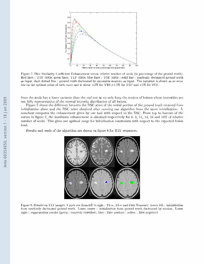
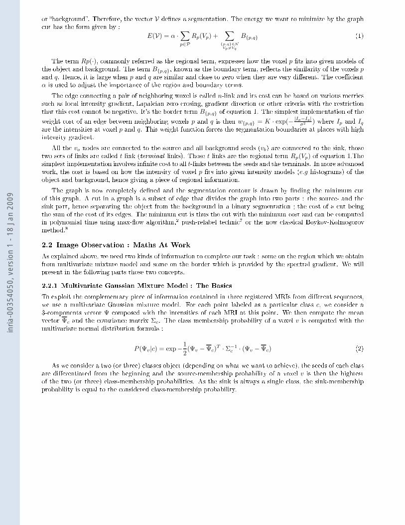
Figure 7. Di e Similarity Coe� ient Enhan ement versus relative number of seeds (in per entage of the ground truth).Red lines : TTF MRIs, green lines: TTP MRIs, blue lines : TGF MRIs ; solid line : randomly de imated ground truthas input, dash dotted line : ground truth de imated by su essive erosions as input. The variation is shown as an errorbar on the optimal point of ea h urve and is about ±2% for TTF,±1.5% for TTP and ±1% fot TGF.from the seeds has a lower varian e than the real one as we only keep the enters of lesions whose intensities arenot fully representative of the normal intensity distribution of all lesions.Figure 7 shows the di�eren e between the DSC s ore of the initial portion of the ground truth retained frominitialisation alone and the DSC s ore obtained after running our algorithm from the same initialisation. Itsomehow omputes the enhan ement given by our tool with respe t to the DSC. From top to bottom of the urves in �gure 7, the maximum enhan ement is obtained respe tively for 6, 8, 11, 14, 16 and 18% of relativenumber of seeds. This gives our optimal range for initialisation onstraints with respe t to the expe ted lesionload.Results and seeds of the algorithm are shown on �gure 8 for TTF sequen es.

Figure 8. Results on TTF images. Upper row from left to right : T1-w, T2-w and Flair Sequen e. Lower left : initialisationfrom randomly de imated ground truth. Lower enter : initialisation from ground truth de imated by erosion. Lowerright : segmentation results (green : orre tly lassi�ed ; blue : false positive ; yellow : false negative)

inria

-003

5405

0, v

ersi

on 1

- 18

Jan

200

9

We then applied the spe tral gradient Graph Cuts on MRIs of patients with tumors. The aim of these testswere to be able to segment a urately the peri-tumoral edema and the tumor itself. The MR sequen es used forthis purpose are T1 and T1 with Gadolinium inje tion images omposed of 182 sli es of 256 x 256 isometri 1mm voxels and an interpolated FLAIR image (original size 704x704x34). As in the pre eding appli ations, the�rst pass gives us the brain mask, then we apply the graph ut for ea h lass of interest (white matter, greymatter, edema and tumor). On the following �gure, we an see that the tumor (in blue) and edema (in darkgrey) regions are well segmented. This result was obtained in roughly 90 se onds. Visual assesment have beenperformed by an expert.Figure 9. Our segmentation (right), T1 image (middle) and Flair image (left).4. CONCLUSION AND FUTURE WORKIn this paper, we have introdu ed the spe tral gradient in the �eld of 3D medi al images. This new, fastand robust multiple images segmentation framework allows us to pro ess multi hannel data from s ale-spa ederivatives.Its optimization by a hierar hi al graph uts has proven to be a urate with very e�e tive results. It om-bines region-based intensity pro essing and ontour-based s ale-spa e approa h in a new way. With su h little omputational time, it allows the user to intera tively orre t the results from a very limited input e�ort.We've built our work on an analogy between RGB hannels and multi-modal MRIs. This method may not beoptimal, espe ially the transform matrix M (cf eq. 6). To �nd the optimal matrix, we ould learn its parametersfrom a supervised pro edure.We propose here a semi-automati but supervising the intensity model of lesions ould give an automati initialisation. Su h models ould be given by the STREM algorithm from Ait-Ali et al.23The next steps of this work will be to run more advan ed validation studies and parti ularly on longitudinaldata sets in order to be able, for instan e, to quantify the evolution of multiple s lerosis lesions and to study thein�uen e of the parameter of the M matrix parameters.REFERENCES[1℄ Greig, D., Porteous, B., and Seheult, A., �Exa t maximum a posteriori estimation for binary images,� Journal of theRoyal Statisti al So iety 51(2), 271�279 (1989).[2℄ Ford, L. and Fulkerson, D., �Maximal �ow through a network,� Canadian Journal of Mathemati s 8, 399�404 (1956).[3℄ Boykov, Y., Veksler, O., and Zabih, R., �Fast approximate energy minimization via graph uts,� IEEE Transa tionson Pattern Analysis and Ma hine Intelligen e 23(11), 1222�1239 (2001).[4℄ Boykov, Y. and Jolly, M.-P., �Intera tive organ segmentation using graph uts,� in [International Conferen e onMedi al Image Computing and Computer-Assisted Intervention ℄, 276�286, Springer-Verlag (2000).[5℄ Boykov, Y. and Jolly, M.-P., �Intera tive graph uts for optimal boundary & region segmentation of obje ts in N-Dimages,� in [International Conferen e on Computer Vision ℄, 1, 105�112 (July 2001).[6℄ Boykov, Y. and Funka-Lea, G., �Graph uts and e� ient N-D images segmentation,� International Journal of Com-puter Vision 70, 109�131 (Nov. 2006).[7℄ Goldberg, A. and Tarjan, A., �A new approa h to the maximum �ow problem,� Journal of the asso iation for omputing Ma hinery 35, 921�940 (10 1988).[8℄ Boykov, Y. and Kolmogorov, V., �An experimental omparison of min- ut/max-�ow algorithms for energy minimiza-tion in vision,� IEEE Transa tions on Pattern Analysis and Ma hine Intelligen e 26, 1124�1137 (Sept. 2004).

inria

-003

5405

0, v

ersi

on 1

- 18

Jan

200

9

[9℄ Geusebroek, J.-M., Dev, A., van den Boomgaard, R., Smeulders, A., Cornelissen, F., and Geerts, H., �Color invariantedge dete tion,� in [S ale-Spa e Theories in Computer Vision ℄, Le ture Notes in Computer S ien e 1252, 459�464(1999).[10℄ Koenderink, J., [Color Spa e ℄, Utre ht University (1998).[11℄ Geusebroek, J.-M., van den Boomgaard, R., Smeulders, A., and Dev, A., �Color and spa e : The spatial stru tureof olor images,� in [IEEE European Conferen e on Computer Vision ℄, Le ture Notes in Computer S ien e 1842,331�341 (2000).[12℄ Lombaert, H., Sun, Y., Grady, L., and Xu, C., �A multilevel banded graph uts method for fast image segmentation,�in [International Conferen e on Computer Vision ℄, 1, 259�265 (O t. 2005).[13℄ Karypis, G. and Kumar, V., �Multilevel k-way partitioning s heme for irregular graphs,� Journal of Parallel andDistributed Computing 48(1), 96�129 (1998).[14℄ Adalsteinsson, D. and Sethian, J.-A., �A fast level set method for propagating interfa es,� Journal of ComputationalPhysi s 118, 269�277 (1995).[15℄ Co os o, C., Kwan, K., and Evans, R., �Brainweb: online interfa e to a 3-d mri simulated brain database,� Neuroim-age 5(4), part 2/4, S425 (1997).[16℄ Ashburner, J. and Friston, K., �Uni�ed segmentation,� Neuroimage 26, 839�851 (2005).[17℄ S herrer, B., Dojat, M., F., F., and Garbay, C., �LOCUS: LO al ooperative Uni�ed Segmentation of MRI BrainS ans,� in [International Conferen e on Medi al Image Computing and Computer-Assisted Intervention ℄, 219�227(2007).[18℄ Bri q, S., Segmentation d'images IRM anatomiques par inféren e bayésienne multimodale et déte tion de lésions,PhD thesis, Université Louis Pasteur de Strasbourg (2008).[19℄ Zijdenbos, A. P., Dawant, B. M., Margolin, R. A., and Palmer, A. C., �Morphometri analysis of white matter lesionsin mr images: Method and validation,� IEEE Transa tions on Medi al Imaging 13(4), 716�724 (1994).[20℄ Van Leemput, K., Maes, F., Vandermeulen, D., Col hester, A., and Suetens, P., �Automated segmentation of multiples lerosis lesions by model outlier dete tion,� IEEE Transa tions on Medi al Imaging 20(8), 677�688 (2001).[21℄ Freifeld, O., Greenspan, H., and Goldberger, J., �Lesion dete tion in noisy MR brain images using onstrained GMMand a tive ontours,� in [IEEE International Symposium on Biomedi al Imaging: From Nano to Ma ro ℄, 596�599(2007).[22℄ Rousseau, F., Blan , F., de Sèze, J., Rumba , L., and Armspa h, J., �An a ontratio approa h for outliers segmen-tation : appli ation to multiple s lerosis in MRI,� in [IEEE International Symposium on Biomedi al Imaging: FromNano to Ma ro ℄, 9�12 (2008).[23℄ Aït-Ali, L., Prima, S., Hellier, P., Carsin, B., Edan, G., and Barillot, C., �STREM: a robust multidimensionalparametri method to segment MS lesions in MRI,� in [International Conferen e on Medi al Image Computing andComputer-Assisted Intervention ℄, Le ture Notes in Computer S ien e 3749, 409�416, Springer Berlin / Heidelberg(O t. 2005).

inria

-003

5405

0, v

ersi

on 1

- 18

Jan

200

9