GPU implementation of Extended Gaussian mixturemodel for Background subtraction

Vu Pham, Vo Dinh Phong, Vu Thanh Hung, Le Hoai BacDepartment of Computer Science

University of ScienceHo Chi Minh City, Viet Nam

{phvu, vdphong, vthung, lhbac}@fit.hcmus.edu.vn

Abstract—Although trivial background subtraction (BGS) al-gorithms (e.g. frame differencing, running average...) can per-form quite fast, they are not robust enough to be used invarious computer vision problems. Some complex algorithmsusually give better results, but are too slow to be appliedto real-time systems. We propose an improved version of theExtended Gaussian mixture model that utilizes the computationalpower of Graphics Processing Units (GPUs) to achieve real-time performance. Experiments show that our implementationrunning on a low-end GeForce 9600GT GPU provides at least10x speedup. The frame rate is greater than 50 frames per second(fps) for most of the tests, even on HD video formats.

Index Terms—Gaussian mixture model, Background subtrac-tion, GPU

I. INTRODUCTION

In many computer vision applications such as human-computer interaction, traffic monitoring, video surveillance...background subtraction (BGS) is widely used as a prepro-cessing step. This is a process to separate or segment out theforeground objects from the background of a video. The fore-ground objects are defined as the parts of the video frame thatchanges and the background is made out of the pixels that stayrelatively constant. In real-life scenarios, however, there aremany factors can affect the video: illumination change, movingobjects in the background, camera moving... In order to takeaccount of those issues, numerous BGS algorithms have beendeveloped. These algorithms are often divided into two classes:parametric models and non-parametric models. Parametricmodels maintain a single background model that is updatedwith each new video frame, while non-parametric models storea buffer of n previous video frames and estimate a backgroundmodel based solely on statistical properties of these frames.Approximated median filtering (AMF) [1], Running Gaussianaverage [2], Gaussian mixture model (GMM) [3]... are some ofcommon parametric models. Some of popular non-parametricmodels are Eigenbackgrounds [4], Kernel density estimator(KDE) [5], Median filtering [6]... Recently, there are somesurveys and comparative studies examined a wide-range ofBGS methods [7], [8], [9], [10]. Some of them [9] focused onlyon computational complexity, memory requirement and theo-retical accuracy, but some others [7], [10], [8] also investigatedthe practical performance and post-processing techniques. Inthose studies, it can be seen that none of the common BGSmethods consistently outperform any other, the choice of BGS

algorithms depends on the specific context that we are workingon.

For most of common pixel-level BGS methods, the scenemodel maintains a probability density function for each pixelindividually. A pixel in a new image is regarded as backgroundif its new value is well described by its density function.Since the intensity value of pixels can change frame by frame,one might want to estimate appropriate values for mean andvariance of underlying distribution of pixel intensities. Thissingle Gaussian model was used by Wren et al. [2]. However,pixel value distributions are often more complex, hence moresophisticated models are necessary to get around under-fittingissue.

In 1997, Friedman and Russell proposed GMM approachfor BGS [11]. Later, efficient update equations are given in[3] by Stauffer and Grimson, and this is often considered asthe exemplary version of GMM for BGS. In [12], the GMMis extended with a hysteresis threshold. The standard GMMupdate equations are extended in [13] to improve the speed ofalteration of the model. All these GMMs use a fixed number ofcomponents. Stenger et al. [14] suggested a method to selectthe number of components of a hidden Markov model in anoff-line training procedure. The GMM update equations arecontinuously improved to simultaneously select the appropri-ate number of components for each pixel on-the-fly, which notonly makes the model adapt fully to the scene, but also reducesthe processing time and improves the segmentation [15], [16].We consider this Extended GMM to be the state of the artin parametric background subtraction techniques. Nonetheless,we observed that the original implementation of Zivkovic [16]is still slow in demanding applications, especially for high-resolution video sequences.

The contemporary Graphics processing units (GPUs) areoptimized for the specific task of rendering images, and canbe very efficient on many data-parallel tasks. However, asopposed to CPUs, which provide more flexibility in programcontrol, GPUs utilize the so-called ’single instruction multipledata’ (SIMD) architecture to perform massively parallel opera-tions. Programs which run on GPU must follow the traditionalgraphics pipeline. This makes difficulties in implementinggeneral algorithms on GPU. In order to obtain maximumspeedup on GPU, one cannot write a multithreaded programas for CPU. Care must be taken to coalesce memory requestsand to minimize the branching factor, as threads on the same

multiprocessor operate concurrently. The Compute UnifiedDevice Architecture (CUDA) from Nvidia [17] and the Close-To-Metal (CTM) from ATI/AMD [18] are such interfacesfor modern GPUs. Lately, many modern applications areincreasingly turning to GPUs for specialized computations[19].

In this report, we present a fast processing version ofExtended GMM using CUDA. We use global memory andconstant memory on GPU for effective computation. We opti-mize memory access pattern to maximize memory throughput,which helps to improve the overall performance dramatically.CUDA streams are also utilized to execute kernel functionasynchronously. These optimization techniques are commonlyused in CUDA developer community and they have very goodeffect on performance of CUDA algorithms.

The first GPU implementation of Stauffer’s and Grimson’salgorithm was proposed by Lee and Jeong in 2006 usingNvidia’s Cg library [20]. Later in 2008, Peter Carr [21]reported an implementation of Stauffer’s and Grimson’s al-gorithm using Apple’s Core Image Kernel Library (CIKL)[22]. He achieved a speedup of 5x with 58 frames per second(fps) on the 352x288 video sequence. However, those worksfocused on improving the original Stauffer’s and Grimson’smethod, while we investigate on Zivkovic’s Extended GMM.On the 400x300 benchmark video, our implementation exe-cutes in more than 980 fps, 13 times faster than the originalimplementation of Zivkovic.

The paper is organized as follows. In the next section, wereview Zivkovic’s Extended GMM algorithm. Section III dis-cusses the implementation on CUDA and various optimizationtechniques which we have used in order to reach the maximumspeedup. In Section IV, we present the experimental resultsand analyze them. Some concluding remarks and directionsfor future work are given in Section V.

II. EXTENDED GAUSSIAN MIXTURE MODEL

The Gaussian Mixture Model stores M separated normaldistributions for each pixel (parameterized by mean µi, vari-ance σ2

i and mixing weight wi, where i = 1, 2, ...,M ) withM typically between 3 and 5 (depending on the complexity ofthe scene). This leads to the following probability distributionfor pixel value It

P (It) =

M∑i=1

wiN (It;µi, σ2i I) (1)

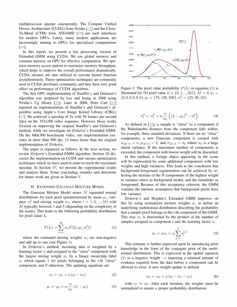
where the estimated mixing weights wi are non-negativeand add up to one (see Figure 1).

In Zivkovic’s method, incoming data is weighted by alearning factor α and assigned to the “close” component withthe largest mixing weight wi by a binary ownership labeloi which equals 1 for pixels belonging to the i-th “close”component, and 0 otherwise. The updating equations are

wi ← wi + α (oi − wi) (2)

µi ← µi + oiα

wi(It − µi) (3)

Figure 1: The pixel value probability P (It) in equation (1) isillustrated for 1D pixel value It ∈ {0, 1, .., 255},M = 3, wi ={0.3, 0.3, 0.4}, µi = {70, 120, 200}, σ2

i = {25, 30, 10}.

σ2i ← σ2

i + oiα

wi

((It − µi)

2 − σ2i

)(4)

As defined in [16], a sample is “close” to a component ifthe Mahalanobis distance from the component falls within,for example, three standard deviations. If there are no “close”components, a new Gaussian component is created withwM+1 = α, µM+1 = It and σM+1 = σ0 where σ0 is a largeinitial variance. If the maximum number of components isexceeded, the component with lowest weight will be discarded.

In this method, a foreign object appearing in the scenewill be represented by some additional components with lowweights and high variances. This leads to the conclusion thatbackground-foreground segmentation can be achieved by se-lecting the mixture of the N components of the highest weightto variance ratios as background model, and the remainder asforeground. Because of this acceptance criterion, the GMMcontains the intrinsic assumption that background pixels havelow variance.

Zivkovic’s and Heijden’s Extended GMM improves onthis by using normalized mixture weights wi to define anunderlying multinomial distribution describing the probabilitythat a sample pixel belongs to the i-th component of the GMM.This way wi is determined by the product of the number ofsamples assigned to component i and the learning factor α:

wi = αni = α

T∑j=1

o(j)i (5)

This estimate is further improved upon by introducing priorknowledge in the form of the conjugate prior of the multi-nomial distribution. This is expressed in the update equation(2) as a negative weight −c imposing a minimal amount ofevidence required from the data before a component can beallowed to exist. A new weight update is defined

wi ← wi + α (oi − wi − cT ) (6)

with cT ≈ αc. After each iteration, the weights must benormalized to ensure a proper probability distribution.

This method can adapt to changing circumstances and awide range of irregular foreground objects being introducedin the scene, while retaining control over the number ofGaussians in the mixtures.

III. EXTENDED GMM ON CUDA

The CUDA environment exposes the SIMD architecture ofthe GPUs by enabling the operation of program kernels ondata grids, divided into multiple blocks consisting of severalthreads. The highest performance is achieved when the threadsavoid divergence and perform the same operation on theirdata elements. The GPU has high computational power butlow memory bandwidth. CUDA threads can access data fromseveral memory spaces during their execution. Each thread hasprivate local memory. Each thread block has shared memoryvisible to all threads of the block. All threads have accessto the same global memory. There are two additional read-only memory spaces: constant and texture memory spaces.Accessing to constant memory and shared memory is generallymuch faster than global memory. However, shared memory islimited in capacity and it is only fast as long as there are nobank conflicts between the threads. This basic knowledge issignificant in developing and considering an implementationon CUDA. The details of CUDA memory hierarchy andCUDA heterogeneous programming model can be found in[17].

A. Basic implementation

In both CPU and GPU implementations, each pixel is pro-cessed independently from each other. This makes ExtendedGMM an embarrassingly parallel algorithm, which can beparallelized by devoting a thread for each pixel. However, thenumber of threads on GPU is limited, while the number ofpixels per frame is various for each video. Our implementationdeals with this by automatically choosing an appropriatenumber of pixels for each thread. When a new frame arrives,the algorithm is run and the background model is updated.Pixels in output image are classified as either foreground orbackground, depends on their intensity value. This process isdepicted in Figure 2.

Figure 2: General execution flow chart of the CPU/GPUimplementation.

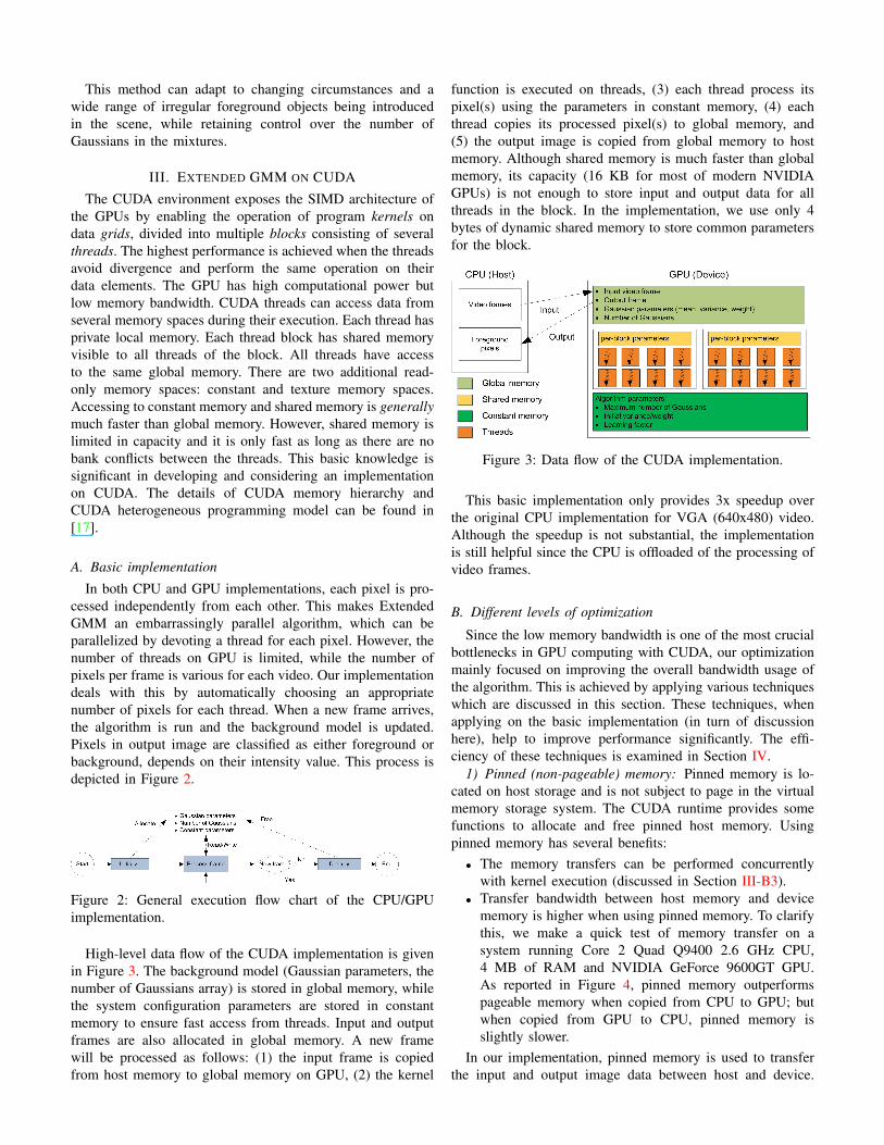
High-level data flow of the CUDA implementation is givenin Figure 3. The background model (Gaussian parameters, thenumber of Gaussians array) is stored in global memory, whilethe system configuration parameters are stored in constantmemory to ensure fast access from threads. Input and outputframes are also allocated in global memory. A new framewill be processed as follows: (1) the input frame is copiedfrom host memory to global memory on GPU, (2) the kernel

function is executed on threads, (3) each thread process itspixel(s) using the parameters in constant memory, (4) eachthread copies its processed pixel(s) to global memory, and(5) the output image is copied from global memory to hostmemory. Although shared memory is much faster than globalmemory, its capacity (16 KB for most of modern NVIDIAGPUs) is not enough to store input and output data for allthreads in the block. In the implementation, we use only 4bytes of dynamic shared memory to store common parametersfor the block.

Figure 3: Data flow of the CUDA implementation.

This basic implementation only provides 3x speedup overthe original CPU implementation for VGA (640x480) video.Although the speedup is not substantial, the implementationis still helpful since the CPU is offloaded of the processing ofvideo frames.

B. Different levels of optimization

Since the low memory bandwidth is one of the most crucialbottlenecks in GPU computing with CUDA, our optimizationmainly focused on improving the overall bandwidth usage ofthe algorithm. This is achieved by applying various techniqueswhich are discussed in this section. These techniques, whenapplying on the basic implementation (in turn of discussionhere), help to improve performance significantly. The effi-ciency of these techniques is examined in Section IV.

1) Pinned (non-pageable) memory: Pinned memory is lo-cated on host storage and is not subject to page in the virtualmemory storage system. The CUDA runtime provides somefunctions to allocate and free pinned host memory. Usingpinned memory has several benefits:

• The memory transfers can be performed concurrentlywith kernel execution (discussed in Section III-B3).

• Transfer bandwidth between host memory and devicememory is higher when using pinned memory. To clarifythis, we make a quick test of memory transfer on asystem running Core 2 Quad Q9400 2.6 GHz CPU,4 MB of RAM and NVIDIA GeForce 9600GT GPU.As reported in Figure 4, pinned memory outperformspageable memory when copied from CPU to GPU; butwhen copied from GPU to CPU, pinned memory isslightly slower.

In our implementation, pinned memory is used to transferthe input and output image data between host and device.

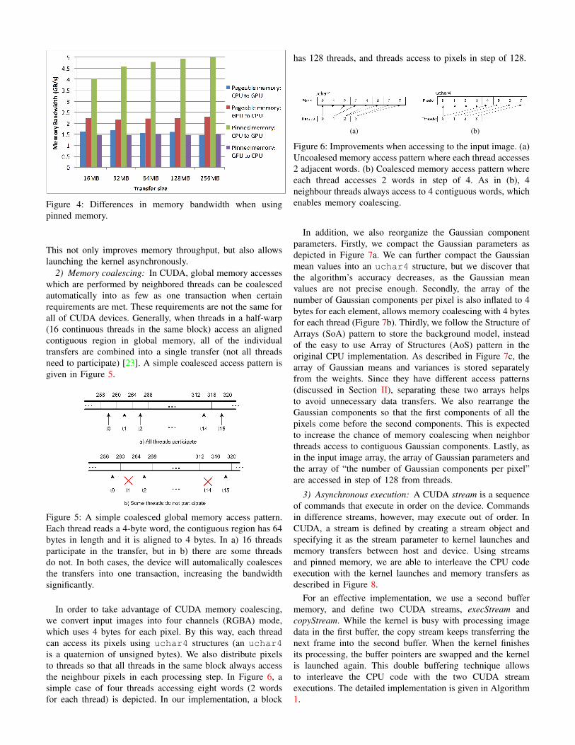
Figure 4: Differences in memory bandwidth when usingpinned memory.

This not only improves memory throughput, but also allowslaunching the kernel asynchronously.

2) Memory coalescing: In CUDA, global memory accesseswhich are performed by neighbored threads can be coalescedautomatically into as few as one transaction when certainrequirements are met. These requirements are not the same forall of CUDA devices. Generally, when threads in a half-warp(16 continuous threads in the same block) access an alignedcontiguous region in global memory, all of the individualtransfers are combined into a single transfer (not all threadsneed to participate) [23]. A simple coalesced access pattern isgiven in Figure 5.

Figure 5: A simple coalesced global memory access pattern.Each thread reads a 4-byte word, the contiguous region has 64bytes in length and it is aligned to 4 bytes. In a) 16 threadsparticipate in the transfer, but in b) there are some threadsdo not. In both cases, the device will automalically coalescesthe transfers into one transaction, increasing the bandwidthsignificantly.

In order to take advantage of CUDA memory coalescing,we convert input images into four channels (RGBA) mode,which uses 4 bytes for each pixel. By this way, each threadcan access its pixels using uchar4 structures (an uchar4is a quaternion of unsigned bytes). We also distribute pixelsto threads so that all threads in the same block always accessthe neighbour pixels in each processing step. In Figure 6, asimple case of four threads accessing eight words (2 wordsfor each thread) is depicted. In our implementation, a block

has 128 threads, and threads access to pixels in step of 128.

(a) (b)

Figure 6: Improvements when accessing to the input image. (a)Uncoalesed memory access pattern where each thread accesses2 adjacent words. (b) Coalesced memory access pattern whereeach thread accesses 2 words in step of 4. As in (b), 4neighbour threads always access to 4 contiguous words, whichenables memory coalescing.

In addition, we also reorganize the Gaussian componentparameters. Firstly, we compact the Gaussian parameters asdepicted in Figure 7a. We can further compact the Gaussianmean values into an uchar4 structure, but we discover thatthe algorithm’s accuracy decreases, as the Gaussian meanvalues are not precise enough. Secondly, the array of thenumber of Gaussian components per pixel is also inflated to 4bytes for each element, allows memory coalescing with 4 bytesfor each thread (Figure 7b). Thirdly, we follow the Structure ofArrays (SoA) pattern to store the background model, insteadof the easy to use Array of Structures (AoS) pattern in theoriginal CPU implementation. As described in Figure 7c, thearray of Gaussian means and variances is stored separatelyfrom the weights. Since they have different access patterns(discussed in Section II), separating these two arrays helpsto avoid unnecessary data transfers. We also rearrange theGaussian components so that the first components of all thepixels come before the second components. This is expectedto increase the chance of memory coalescing when neighborthreads access to contiguous Gaussian components. Lastly, asin the input image array, the array of Gaussian parameters andthe array of “the number of Gaussian components per pixel”are accessed in step of 128 from threads.

3) Asynchronous execution: A CUDA stream is a sequenceof commands that execute in order on the device. Commandsin difference streams, however, may execute out of order. InCUDA, a stream is defined by creating a stream object andspecifying it as the stream parameter to kernel launches andmemory transfers between host and device. Using streamsand pinned memory, we are able to interleave the CPU codeexecution with the kernel launches and memory transfers asdescribed in Figure 8.

For an effective implementation, we use a second buffermemory, and define two CUDA streams, execStream andcopyStream. While the kernel is busy with processing imagedata in the first buffer, the copy stream keeps transferring thenext frame into the second buffer. When the kernel finishesits processing, the buffer pointers are swapped and the kernelis launched again. This double buffering technique allowsto interleave the CPU code with the two CUDA streamexecutions. The detailed implementation is given in Algorithm1.

(a) Compaction of Gaussian meanvalues into a float4 structure.

(b) Inflation of the “number ofGaussian components per pixel” ar-ray.

(c) Reorganizing the background model using the SoA pattern. Separatingweights from means and variances helps avoid unnecessary memorytransfer, since they have different access patterns from threads. ReorderingGaussian components so that the first components come before the secondcomponents helps to increase the chance of memory coalescing.

Figure 7: Improvements on storing the Gaussian parametersarrays.

Figure 8: Timeline for asynchronous execution. In thecopy stream (the second row), transfers are performedby cudaMemcpyAsync; while CPU (the third row) usesmemcpy as usual.

IV. EXPERIMENTAL RESULTS

The CPU and GPU implementations are executed on thedataset from the VSSN 2006 competition [24] to compare therobustness, and on the PETS2009 [25] dataset to evaluate thespeedup. The VSSN2006 dataset contains various 384x240semi-synthetic (synthetic foreground object moving over areal background) AVI video sequences and the correspondingground truth sequences. We chose video 2, video 4 and video 8for evaluation. Video 2 has 500 frames with a relatively staticindoor scene. Video 4 has 820 frames and is more dynamicwith swaying leafs in the background. Video 8 (1920 frames)uses the same background with video 2, but at the end of thesequence, lamps are turned on and the illumination is changed.PETS2009 is a set of 768x576 JPEG image sequences inoutdoor condition. It has 4 subsets, each subset containsseveral sequences and each sequence contains from 4 up to8 views. We choose view 1 and view 2 from S1.L1 (subject1, sequence 1) scenario, view 1 from S1.L2 scenario to testthe performance of the implementations. All experiments inthis section are performed on a system running Core 2 QuadQ9400 2.6 GHz CPU (4 GB of RAM) and GeForce 9600GT

Algorithm 1 Code segment that implements the asynchronousexecution in CUDA.

Input: GmmModel, inputImgOutput: outputImgBegin// wait for the copyStreamSynchronize(copyStream)

// CPU code: copy to/from pinned memorycopy(pinnedIn, inputImg, ...)copy(outputImg, pinnedOut, ...)

// wait for the execStreamSynchronize(execStream)

// swap pointersswap(globalInMemory, globalInMemory2)swap(globalOutMemory, globalOutMemory2)

// copyStream: copy to/from GPU global memoryCopyAsync(globalInMemory, pinnedIn, ..., copyStream)CopyAsync(pinnedOut, globalOutMemory,..., copyStream)

// execStream: launch the kernelUpdateGmmModel<<<..., execStream>>> (globalInMemory2,

globalOutMemory2)End

GPU. Although the CPU implementation is not multithreaded,we still execute it on four cores to get the best performance.

A. Optimization levels and Occupancy

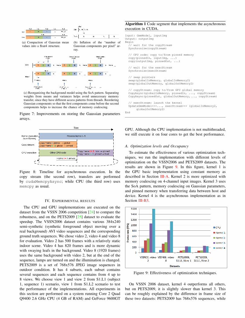
To estimate the effectiveness of various optimization tech-niques, we run the implementation with different levels ofoptimization on the VSSN2006 and PETS2009 datasets. Theresults are shown in Figure 9. In this figure, kernel 1 isthe GPU basic implementation using constant memory asdescribed in Section III-A. Kernel 2 is more optimized withmemory coalescing on 4-channel input images. Kernel 3 usesthe SoA pattern, memory coalescing on Gaussian parameters,and pinned memory when transferring data between host anddevice. Kernel 4 is the asynchronous implementation as inSection III-B3.

Figure 9: Effectiveness of optimization techniques.

On VSSN 2006 dataset, kernel 4 outperforms all others,but on PETS2009, it is slightly slower than kernel 3. Thiscan be roughly explained by the difference in frame size ofthese two datasets: PETS2009 has 768x576 sequences, while

VSSN2006 contains smaller 384x240 video sequences. Theasynchronous implementation in kernel 4 requires more timeto transfer large data between host and device, leads to thedecrement in frame rate. Nevertheless, we prefer kernel 4since it is better in interleaving the CPU processing into theGPU processing time. In this section, we use kernel 4 for allremaining experiments.

In CUDA, the multiprocessor occupancy is the ratio ofactive warps to the maximum number of warps supportedon a multiprocessor of the GPU. It depends on number ofthreads per block, number of registers per thread, capacityof shared memory per block that a kernel uses, and oncompute capability of the device. Our implementation uses128 threads per block, 20 registers per thread and 36 bytesof shared memory per block. The implementation is executedon GeForce 9600GT which supports compute capability 1.1.Thus, the kernel has occupancy of 0.5. This configuration isdetermined experimentally. When attempting to increase theoccupancy by using less registers per thread and more/lessthreads per block, we notice that the overall performance falls.

B. Robustness

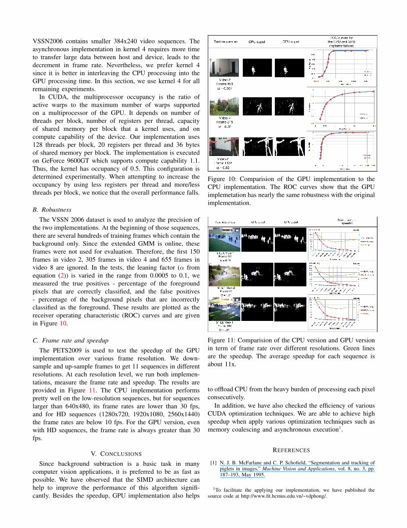
The VSSN 2006 dataset is used to analyze the precision ofthe two implementations. At the beginning of those sequences,there are several hundreds of training frames which contain thebackground only. Since the extended GMM is online, theseframes were not used for evaluation. Therefore, the first 150frames in video 2, 305 frames in video 4 and 655 frames invideo 8 are ignored. In the tests, the leaning factor (α fromequation (2)) is varied in the range from 0.0005 to 0.1, wemeasured the true positives - percentage of the foregroundpixels that are correctly classified, and the false positives- percentage of the background pixels that are incorrectlyclassified as the foreground. These results are plotted as thereceiver operating characteristic (ROC) curves and are givenin Figure 10.

C. Frame rate and speedup

The PETS2009 is used to test the speedup of the GPUimplementation over various frame resolution. We down-sample and up-sample frames to get 11 sequences in differentresolutions. At each resolution level, we run both implemen-tations, measure the frame rate and speedup. The results areprovided in Figure 11. The CPU implementation performspretty well on the low-resolution sequences, but for sequenceslarger than 640x480, its frame rates are lower than 30 fps,and for HD sequences (1280x720, 1920x1080, 2560x1440)the frame rates are below 10 fps. For the GPU version, evenwith HD sequences, the frame rate is always greater than 30fps.

V. CONCLUSIONS

Since background subtraction is a basic task in manycomputer vision applications, it is preferred to be as fast aspossible. We have observed that the SIMD architecture canhelp to improve the performance of this algorithm signifi-cantly. Besides the speedup, GPU implementation also helps

Figure 10: Comparision of the GPU implementation to theCPU implementation. The ROC curves show that the GPUimplemetation has nearly the same robustness with the originalimplementation.

Figure 11: Comparision of the CPU version and GPU versionin term of frame rate over different resolutions. Green linesare the speedup. The average speedup for each sequence isabout 11x.

to offload CPU from the heavy burden of processing each pixelconsecutively.

In addition, we have also checked the efficiency of variousCUDA optimization techniques. We are able to achieve highspeedup when apply various optimization techniques such asmemory coalescing and asynchronous execution1.

REFERENCES

[1] N. J. B. McFarlane and C. P. Schofield, “Segmentation and tracking ofpiglets in images,” Machine Vision and Applications, vol. 8, no. 3, pp.187–193, May 1995.

1To facilitate the applying our implementation, we have published thesource code at http://www.fit.hcmus.edu.vn/~vdphong/.

[2] C. Wren, A. Azarbayejani, T. Darrell, and A. Pentland, “Pfinder: real-time tracking of the human body,” IEEE Transactions on PatternAnalysis and Machine Intelligence, vol. 19, no. 7, pp. 780–785, July1997.

[3] C. Stauffer and W. E. L. Grimson, “Adaptive Background MixtureModels for Real-Time Tracking,” Proc. CVPR, 1999.

[4] N. Oliver, B. Rosario, and A. Pentland, “A Bayesian computer visionsystem for modeling human interactions,” IEEE Transactions on PatternAnalysis and Machine Intelligence, vol. 22, no. 8, pp. 831–843, 2000.

[5] A. Elgammal, D. Harwood, and L. Davis, “Non-parametric Model forBackground Subtraction,” in ECCV, 2000, pp. 751–767.

[6] S. Calderara, R. Melli, A. Prati, and R. Cucchiara, “Reliable backgroundsuppression for complex scenes,” Proceedings of the 4th ACM interna-tional workshop on Video surveillance and sensor networks - VSSN ’06,p. 211, 2006.

[7] Y. Benezeth, P. Jodoin, B. Emile, H. Laurent, and C. Rosenberger, “Re-view and evaluation of commonly-implemented background subtractionalgorithms,” 2008 19th International Conference on Pattern Recognition,pp. 1–4, December 2008.

[8] D. H. Parks and S. S. Fels, Evaluation of Background SubtractionAlgorithms with Post-Processing. IEEE, September 2008.

[9] M. Piccardi, “Background subtraction techniques: a review,” 2004 IEEEInternational Conference on Systems, Man and Cybernetics (IEEE Cat.No.04CH37583), pp. 3099–3104, 2004.

[10] R. J. Radke, S. Andra, O. Al-Kofahi, and B. Roysam, “Image changedetection algorithms: a systematic survey,” IEEE transactions on imageprocessing : a publication of the IEEE Signal Processing Society,vol. 14, no. 3, pp. 294–307, March 2005.

[11] N. Friedman and S. Russell, “Image segmentation in video sequences: Aprobabilistic approach,” in Thirteenth Conf. on Uncertainty in ArtificialIntelligence, 1997, pp. 175–181.

[12] P. W. Power and J. A. Schoonees, “Understanding Background MixtureModels for Foreground Segmentation,” Image and Vision Computing,no. November, 2002.

[13] P. Kaewtrakulpong and R. Bowden, “An Improved Adaptive BackgroundMixture Model for Real- time Tracking with Shadow Detection,” inProc. 2nd European Workshop on Advanced Video Based SurveillanceSystems, AVBS01. Kluwer Academic, 2001, pp. 1–5.

[14] B. Stenger, V. Ramesh, N. Paragios, F. Coetzee, and J. Buhmann, “Topol-ogy free hidden Markov models: application to background modeling,”Proceedings Eighth IEEE International Conference on Computer Vision.ICCV 2001, vol. 00, no. C, pp. 294–301, 2001.

[15] Z. Zivkovic, “Improved adaptive gaussian mixture model for backgroundsubtraction,” Proceedings of the 17th International Conference on Pat-tern Recognition, 2004. ICPR 2004., no. 2, pp. 28–31, 2004.

[16] Z. Zivkovic and F. van der Heijden, “Efficient adaptive density estima-tion per image pixel for the task of background subtraction,” PatternRecognition Letters, vol. 27, no. 7, pp. 773–780, May 2006.

[17] NVIDIA Corporation, “NVIDIA CUDA Programming Guide,” 2007.[18] AMD/ATI, “ATI CTM (Close to Mental) Guide,” 2007.[19] J. Fung, “Advances in GPU-based Image Processing and Computer

Vision,” in SIGGRAPH, 2009.[20] S.-j. Lee and C.-s. Jeong, “Real-time Object Segmentation based on

GPU,” 2006 International Conference on Computational Intelligenceand Security, pp. 739–742, November 2006.

[21] P. Carr, GPU Accelerated Multimodal Background Subtraction. DigitalImage Computing: Techniques and Applications, December 2008.

[22] Apple Inc., “Core Image Programming Guide,” 2008.[23] NVIDIA Corporation, “NVIDIA CUDA Best Practices Guide,” 2010.[24] “VSSN 2006 Competition,” 2006. [Online]. Available: http://mmc36.

informatik.uni-augsburg.de/VSSN06_OSAC/[25] “PETS 2009 Benchmark Data,” 2009. [Online]. Available: http:

//www.cvg.rdg.ac.uk/PETS2009/a.html