Entropy 2009, 11, 513 - 528; doi:10.3390/e11030513

OPEN ACCESS

entropyISSN 1099-4300

www.mdpi.com/journal/entropy

Article

Scale-Based Gaussian Coverings: Combining Intra and InterMixture Models in Image SegmentationFionn Murtagh 1,2,?, Pedro Contreras 2 and Jean-Luc Starck 3,4

1 Science Foundation Ireland, Wilton Park House, Wilton Place, Dublin 2, Ireland2 Department of Computer Science, Royal Holloway University of London, Egham TW20 0EX, UK;

E-Mail: pedro@cs.rhul.ac.uk3 CEA-Saclay, DAPNIA/SEDI-SAP, Service d’Astrophysique, 91191 Gif sur Yvette, France;

E-Mail: jstarck@cea.fr4 Laboratoire AIM (UMR 7158), CEA/DSM-CNRS, Universite Paris Diderot, Diderot, IRFU,

SEDI-SAP, Service d’Astrophysique, Centre de Saclay, F-91191 Gif-Sur-Yvette cedex, France

? Author to whom correspondence should be addressed: E-Mail: fmurtagh@acm.org;Tel.: +44 1784 443429; Fax: +44 1784 439786.

Received: 1 September 2009 / Accepted: 14 September 2009 / Published: 24 September 2009

Abstract: By a “covering” we mean a Gaussian mixture model fit to observed data.Approximations of the Bayes factor can be availed of to judge model fit to the data withina given Gaussian mixture model. Between families of Gaussian mixture models, we proposethe Renyi quadratic entropy as an excellent and tractable model comparison framework.We exemplify this using the segmentation of an MRI image volume, based (1) on a directGaussian mixture model applied to the marginal distribution function, and (2) Gaussianmodel fit through k-means applied to the 4D multivalued image volume furnished by thewavelet transform. Visual preference for one model over another is not immediate. TheRenyi quadratic entropy allows us to show clearly that one of these modelings is superior tothe other.

Keywords: image segmentation; clustering; model selection; minimum description length;Bayes factor; Renyi entropy; Shannon entropy

Entropy 2009, 11 514

1. Introduction

We begin with some terminology used. Segments are contiguous clusters. In an imaging context,this means that clusters contain adjacent or contiguous pixels. For typical 2D (two-dimensional) images,we may also consider the 1D (one-dimensional) marginal which provides an empirical estimate of thepixel (probability) density function or PDF. For 3D (three-dimensional) images, we can consider 2Dmarginals, based on the voxels that constitute the 3D image volume, or also a 1D overall marginal.An image is representative of a signal. More loosely a signal is just data, mostly here with neccessarysequence or adjacency relationships. Often we will use interchangeably the terms image, image volumeif relevant, signal and data.

The word “model” is used, in general, in many senses–statistical [1], mathematical, physical models;mixture model; linear model; noise model; neural network model; sparse decomposition model; even,in different senses, data model. In practice, firstly and foremostly for algorithmic tractability, modelsof whatever persuasion tend to be homogeneous. In this article we wish to broaden the homogeneousmixture model framework in order to accommodate heterogeneity at least as relates to resolution scale.Our motivation is to have a rigorous model-based approach to data clustering or segmentation, that alsoand in addition encompasses resolution scale.

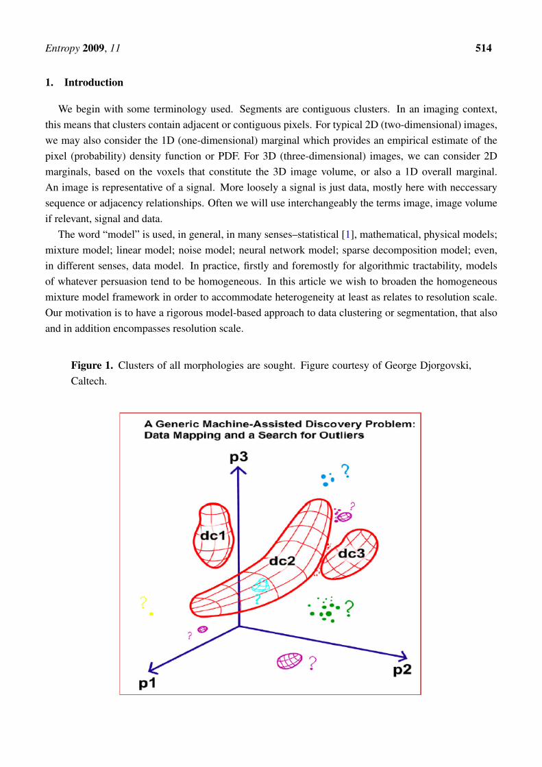
Figure 1. Clusters of all morphologies are sought. Figure courtesy of George Djorgovski,Caltech.

Entropy 2009, 11 515

In Figure 1 [2], the clustering task is portrayed in its full generality. One way to address it is to buildup parametrized clusters, for example using a Gaussian mixture model (GMM), so that the cluster “pods”are approximated by the mixture made up of the cluster component “peas” (a viewpoint expressed byA.E. Raftery, quoted in [3]).

A step beyond a pure “peas” in a “pod” approach to clustering is a hierarchical approach. Applicationspecialists often consider hierarchical algorithms as more versatile than their partitional counterparts(for example, k-means or Gaussian mixture models) since the latter tend to work well only on datasets having isotropic clusters [4]. So in [5], we segmented astronomical images of different observingfilters, that had first been matched such that they related to exactly the same fields of view and pixelresolution. For the segmentation we used a Markov random field and Gaussian mixture model; followedby a within-segment GMM clustering on the marginals. Further within-cluster marginal clustering couldbe continued if desired. For model fit, we used approximations of the Bayes factor: the pseudo-likelihoodinformation criterion to start with, and for the marginal GMM work, a Bayesian information criterion.This hierarchical- or tree-based approach is rigorous and we do not need to go beyond the Bayes factormodel evaluation framework. The choice of segmentation methods used was due to the desire to usecontiguity or adjacency information whenever possible, and when not possible to fall back on use ofthe marginal. This mixture of segmentation models is a first example of what we want to appraise inthis work.

What now if we cannot (or cannot conveniently) match the images beforehand? In that case, segmentsor clusters in one image will not necessarily correspond to corresponding pixels in another image. Thatis a second example of where we want to evaluate different families of models.

A third example of what we want to cater for in this work is the use of wavelet transforms tosubstitute for spatial modeling (e.g., Markov random field modeling). In this work one point ofdeparture is a Gaussian mixture model (GMM) with model selection using the Bayes informationcriterion (BIC) approximation to the Bayes factor. We extend this to a new hierarchical context.We use GMMs on resolution scales of a wavelet transform. The latter is used to provide resolutionscale. Between resolution scales we do not seek a strict subset or embedding relationship over fittedGaussians, but instead accept a lattice relation. We focus in particular on the global quality of fit of thiswavelet-transform based Gaussian modeling. We show that a suitable criterion of goodness of fit forcross-model family evaluations is given by Renyi quadratic entropy.

1.1. Outline of the Article

In Section 2 we review briefly how modeling, with Gaussian mixture modeling in mind, is mappedinto information.

In Section 3 we motivate Gaussian mixture modeling as a general clustering approach.In Section 4 we introduce entropy and focus on the additivity property. This property is importatant

to us in the following context. Since hierarchical cluster modeling, not well addressed or supported byGaussian mixture modeling, is of practical importance we will seek to operationalize a wavelet transformapproach to segmentation. The use of entropy in this context is discussed in Section 5.

The fundamental role of Shannon entropy together with some other definitions of entropy in signaland noise modeling is reviewed in Section 6. Signal and noise modeling are potentially usable for

Entropy 2009, 11 516

image segmentation.For the role of entropy in image segmentation, section 2 presented the state of the art

relative to Gaussian mixture modeling; and Section 6 presented the state of the art relative to(segmentation-relevant) filtering.

What if we have segmentations obtained through different modelings? Section 7 addresses thisthrough the use of Renyi quadratic entropy. Finally, Section 8 presents a case study.

2. Minimum Description Length and Bayes Information Criterion

For what we may term a homogenous modeling framework, the minimum description length, MDL,associated with Shannon entropy [6], will serve us well. However as we will now describe it does notcater for hierarchically embedded segments or clusters. An example of where hierarchical embedding,or nested clusters, come into play can be found in [5].

Following Hansen and Yu [7], we consider a model class, Θ, and an instantiation of this involvingparameters θ to be estimated, yielding θ. We have θ ∈ Rk so the parameter space is k-dimensional. Ourobservation vectors, of dimension m, and of cardinality n, are defined as: X = {xi|1 ≤ i ≤ n}. Amodel, M , is defined as f(X|θ), θ ∈ Θ ⊂ Rk, X = {xi|1 ≤ i ≤ n}, xi ∈ Rm, X ⊂ Rm. The maximumlikelihood estimator (MLE) of θ is θ: θ = argmaxθf(X|θ).

Using Shannon information, the description length of X based on a set of parameter values θ is:− log f(X|θ). We need to transmit parameters also (as, for example, in vector quantization). So overallcode length is: − log f(X|θ) + L(θ). If the number of parameters is always the same, then L(θ) canbe constant. Minimizing − log f(X|θ) over θ is the same as maximizing f(X|θ), so if L(θ) is constant,then MDL (minimum description length) is identical to maximum likelihood, ML.

The MDL information content of the ML, or equally Bayesian maximum a posteriori (MAP) estimate,is the code length of − log f(X|θ) + L(θ). First, we need to encode the k coordinates of θ, where k isthe (Euclidean) dimension of the parameter space. Using the uniform encoder for each dimension, theprecision of coding is then 1/

√n implying that the magnitude of the estimation error is 1/

√n. So the

price to be paid for communicating θ is k · (− log 1/√n) = k

2log n nats [7]. Going beyond the uniform

coder is also possible with the same outcome.In summary, MDL with simple suppositions here (in other circumstances we could require more than

two stages, and consider other coders) is the sum of code lengths for (i) encoding data using a givenmodel; and (ii) transmitting the choice of model. The outcome is minimal − log f(X|θ) + k

2log n.

In the Bayesian approach we assign a prior to each model class, and then we use the overall posteriorto select the best model. Schwarz’s Bayesian Information Criterion (BIC), which approximates the Bayesfactor of posterior ratios, takes the form of the same penalized likelihood,− log f(X|θ) + k

2log n, where

θ = ML or MAP estimate of θ. See [8] for case studies using BIC.

3. Segmentation of Arbitrary Signal through a Gaussian Mixture Model

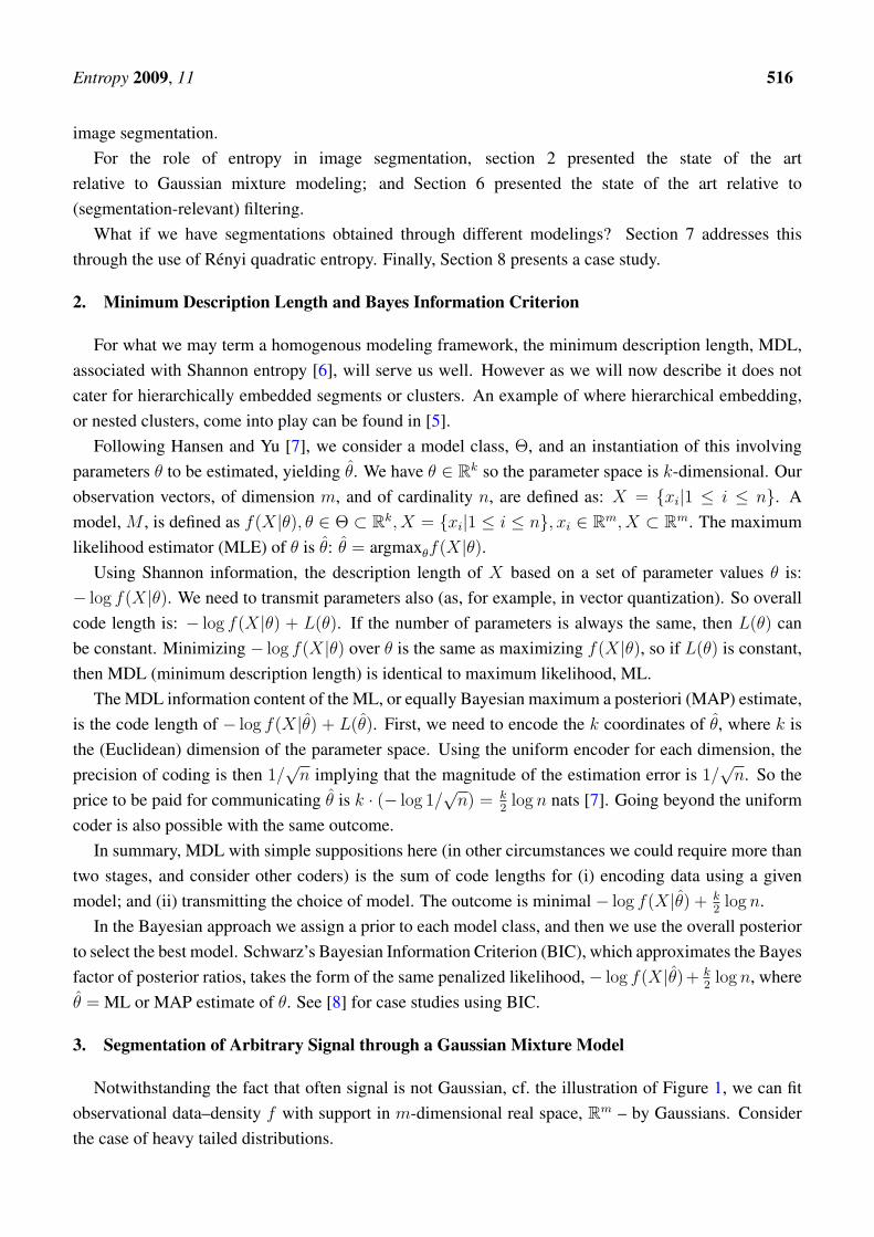
Notwithstanding the fact that often signal is not Gaussian, cf. the illustration of Figure 1, we can fitobservational data–density f with support in m-dimensional real space, Rm – by Gaussians. Considerthe case of heavy tailed distributions.

Entropy 2009, 11 517

Heavy tailed probability distributions, examples of which include long memory or 1/f processes(appropriate for financial time series, telecommunications traffic flows, etc.) can be modeled as ageneralized Gaussian distribution (GGD, also known as power exponential, α-Gaussian distribution,or generalized Laplacian distribution):

f(x) =β

2αΓ(1/β)exp−(| x | /α)β

where– scale parameter, α, represents the standard deviation,– the gamma function, Γ(a) =

∫∞0xa−1e−xdx, and

– shape parameter, β, is the rate of exponential decay, β > 0.A value of β = 2 gives us a Gaussian distribution. A value of β = 1 gives a double exponential or

Laplace distribution. For 0 < β < 2, the distribution is heavy tailed. For β > 2, the distribution islight tailed.

Heavy tailed noise can be modeled by a Gaussian mixture model with enough terms [9]. Similarly, inspeech and audio processing, low-probability and large-valued noise events can be modeled as Gaussiancomponents in the tail of the distribution. A fit of this fat tail distribution by a Gaussian mixture modelis commonly carried out [10]. As in Wang and Zhao [10], one can allow Gaussian component PDFsto recombine to provide the clusters which are sought. These authors also found that using priors withheavy tails, rather than using standard Gaussian priors, gave more robust results. But the benefit appearsto be very small.

Gaussian mixture modeling of heavy tailed noise distributions, e.g. genuine signal and flicker or pinknoise constituting a heavy tail in the density, is therefore feasible. A solution is provided by a weightedsum of Gaussian densities often with decreasing weights corresponding to increasing variances. Mixingproportions for small (tight) variance components are large (e.g., 0.15 to 0.3) whereas very large variancecomponents have small mixing proportions.

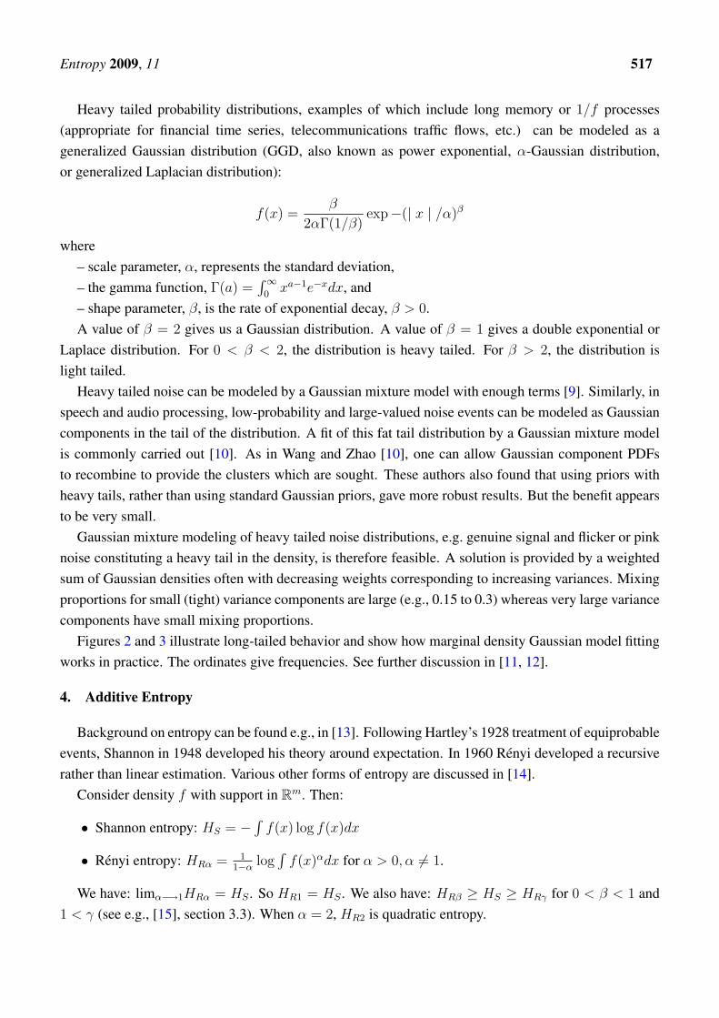
Figures 2 and 3 illustrate long-tailed behavior and show how marginal density Gaussian model fittingworks in practice. The ordinates give frequencies. See further discussion in [11, 12].

4. Additive Entropy

Background on entropy can be found e.g., in [13]. Following Hartley’s 1928 treatment of equiprobableevents, Shannon in 1948 developed his theory around expectation. In 1960 Renyi developed a recursiverather than linear estimation. Various other forms of entropy are discussed in [14].

Consider density f with support in Rm. Then:

• Shannon entropy: HS = −∫f(x) log f(x)dx

• Renyi entropy: HRα = 11−α log

∫f(x)αdx for α > 0, α 6= 1.

We have: limα−→1HRα = HS . So HR1 = HS . We also have: HRβ ≥ HS ≥ HRγ for 0 < β < 1 and1 < γ (see e.g., [15], section 3.3). When α = 2, HR2 is quadratic entropy.

Entropy 2009, 11 518

Figure 2. Upper left: long-tailed histogram of marginal density of product of wavelet scales4 and 5 of a 512 × 512 Lena image. Upper right, lower left, and lower right: histograms ofclasses 1, 2 and 3. These panels exemplify a nested model.

Both Shannon and Renyi quadratic entropy are additive, a property which will be availed of byus below for example when we we define entropy for a linear transform, i.e., an additive, invertibledecomposition.

To show this, let us consider a system decomposed into independent events, A, B.So p(AB) (alternatively written: p(A&B) or p(A + B)) = p(A)p(B). Shannon information is then

IABS = − log p(AB) = − log p(A) − log p(B), so the information of independent events is additive.Multiplying across by p(AB), and taking p(AB) = p(A) when considering only event A and similarlyfor B, leads to additivity of Shannon entropy for independent events, HAB

S = HAS +HB

S .Similarly for Renyi quadratic entropy we use p(AB) = p(A)p(B) and we have:

− log p2(AB) = −2 log p(AB) = −2 log (p(A)p(B)) = −2 log p(A) − 2 log p(B) = − log p2(A) −log p2(B).

5. The Entropy of a Wavelet Transformed Signal

The wavelet transform is a resolution-based decomposition–hence with an in-built spatial model: seee.g., [16, 17].

A redundant wavelet transform is most appropriate, even if decimated alternatives can be consideredstraightforwardly too. This is because segmentation, taking information into account at all availableresolution scales, simply needs all available information. A non-redundant (decimated, e.g., pyramidal)wavelet transform is most appropriate for compression objectives, but it can destroy through aliasing

Entropy 2009, 11 519

potentially important faint features.

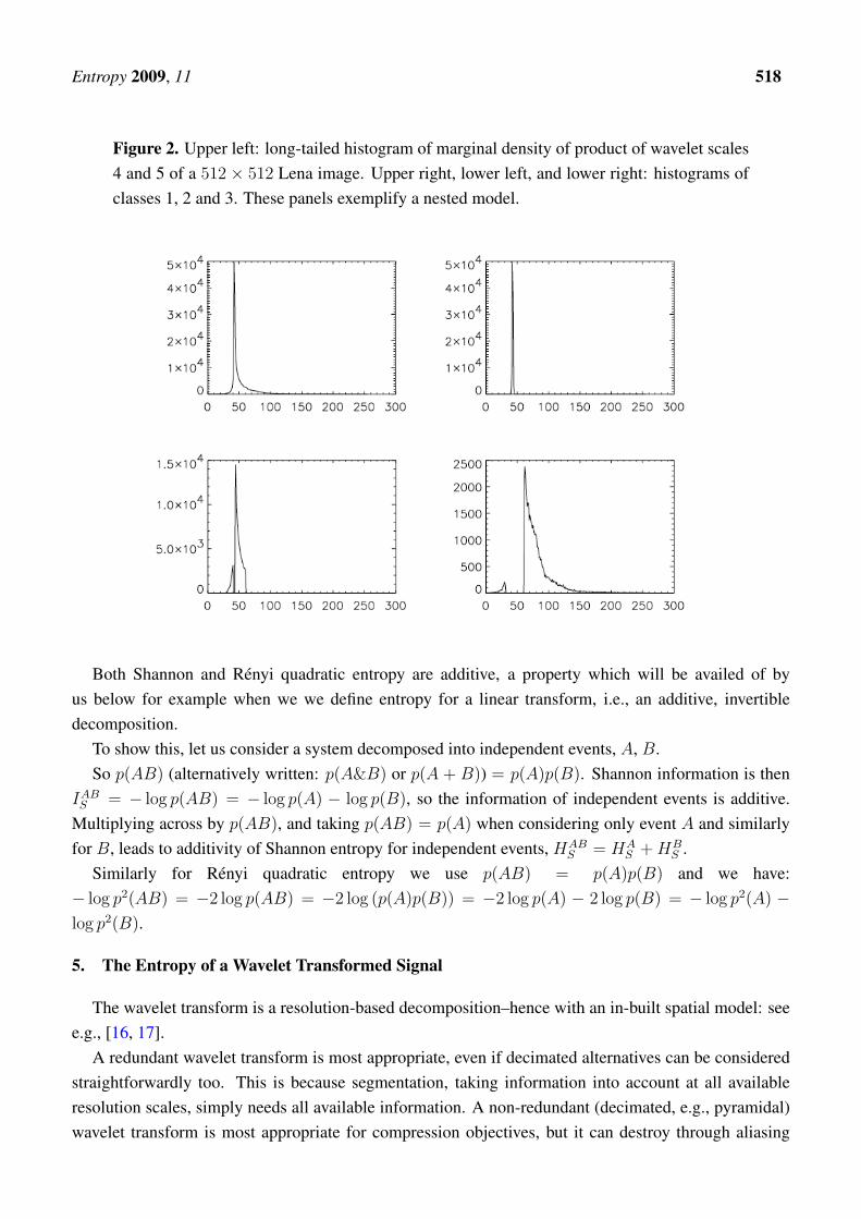
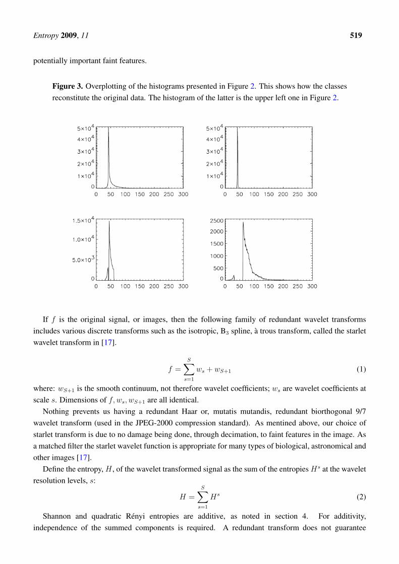
Figure 3. Overplotting of the histograms presented in Figure 2. This shows how the classesreconstitute the original data. The histogram of the latter is the upper left one in Figure 2.

If f is the original signal, or images, then the following family of redundant wavelet transformsincludes various discrete transforms such as the isotropic, B3 spline, a trous transform, called the starletwavelet transform in [17].

f =S∑s=1

ws + wS+1 (1)

where: wS+1 is the smooth continuum, not therefore wavelet coefficients; ws are wavelet coefficients atscale s. Dimensions of f, ws, wS+1 are all identical.

Nothing prevents us having a redundant Haar or, mutatis mutandis, redundant biorthogonal 9/7wavelet transform (used in the JPEG-2000 compression standard). As mentined above, our choice ofstarlet transform is due to no damage being done, through decimation, to faint features in the image. Asa matched filter the starlet wavelet function is appropriate for many types of biological, astronomical andother images [17].

Define the entropy, H , of the wavelet transformed signal as the sum of the entropiesHs at the waveletresolution levels, s:

H =S∑s=1

Hs (2)

Shannon and quadratic Renyi entropies are additive, as noted in section 4. For additivity,independence of the summed components is required. A redundant transform does not guarantee

Entropy 2009, 11 520

independence of resolution scales, s = 1, 2, . . . , S. However in practice we usually have approximateindependence. Our argument in favor of bypassing indepence of resolution scales is based on thepractical and interpretation-related benefits of doing so.

Next we will review the Shannon entropy used in this context. Then we will introduce a newapplication of the Renyi quadratic entropy, again in this wavelet transform context.

6. Entropy Based on a Wavelet Transform and a Noise Model

Image filtering allows, as a special case, thresholding and reading off segmented regions. Suchapproaches have been used for very fast – indeed one could say with justice, turbo-charged–clustering.See [18, 19].

Noise models are particularly important in the physical sciences (cf. CCD, charge-coupled device,detectors) and the following approach was developed in [20]. Observed data f in the physical sciencesare generally corrupted by noise, which is often additive and which follows in many cases a Gaussiandistribution, a Poisson distribution, or a combination of both. Other noise models may also be considered.Using Bayes’ theorem to evaluate the probability distribution of the realization of the original signal g,knowing the data f , we have:

p(g|f) =p(f |g).p(g)

p(f)(3)

p(f |g) is the conditional probability distribution of getting the data f given an original signal g, i.e.,it represents the distribution of the noise. It is given, in the case of uncorrelated Gaussian noise withvariance σ2, by:

p(f |g) = exp

(−∑pixels

(f − g)2

2σ2

)(4)

The denominator in Equation (3) is independent of g and is considered as a constant (stationary noise).p(g) is the a priori distribution of the solution g. In the absence of any information on the solution gexcept its positivity, a possible course of action is to derive the probability of g from its entropy, whichis defined from information theory.

If we know the entropy H of the solution (we describe below different ways to calculate it), we deriveits probability by:

p(g) = exp(−αH(g)) (5)

Given the data, the most probable image is obtained by maximizing p(g|f). This leads to algorithmsfor noise filtering and to deconvolution [16].

We need a probability density p(g) of the data. The Shannon entropy, HS [21], is the summing of thefollowing for each pixel,

HS(g) = −Nb∑k=1

pk log pk (6)

Entropy 2009, 11 521

where X = {g1, ..gn} is an image containing integer values, Nb is the number of possible values of agiven pixel gk (256 for an 8-bit image), and the pk values are derived from the histogram of g as pk = mk

n,

where mk is the number of occurrences in the histogram’s kth bin.The trouble with this approach is that, because the number of occurrences is finite, the estimate pk

will be in error by an amount proportional tom− 1

2k [22]. The error becomes significant whenmk is small.

Furthermore this kind of entropy definition is not easy to use for signal restoration, because its gradientis not easy to compute. For these reasons, other entropy functions are generally used, including:

• Burg [23]:

HB(g) = −n∑k=1

ln(gk) (7)

• Frieden [24]:

HF (g) = −n∑k=1

gk ln(gk) (8)

• Gull and Skilling [25]:

HG(g) =n∑k=1

gk −Mk − gk ln

(gkMk

)(9)

where M is a given model, usually taken as a flat image

In all definitions n is the number of pixels, and k represents an index pixel. For the three entropiesabove, unlike Shannon’s entropy, a signal has maximum information value when it is flat. The sign hasbeen inverted (see Equation (5)), to arrange for the best solution to be the smoothest.

Now consider the entropy of a signal as the sum of the information at each scale of its wavelettransform, and the information of a wavelet coefficient is related to the probability of it being due tonoise. Let us look at how this definition holds up in practice. Denoting h the information relative to asingle wavelet coefficient, we define:

H(X) =l∑

j=1

nj∑k=1

h(wj,k) (10)

with the information of a wavelet coefficient, h(wj,k) = − ln p(wj,k), (Burg’s definition rather thanShannon’s). l is the number of scales, and nj is the number of samples in wavelet band (scale) j. ForGaussian noise, and recalling that wavelet coefficients at a given resolution scale are of zero mean,we get

h(wj,k) =w2j,k

2σ2j

+ constant (11)

where σj is the noise at scale j. When we use the information in a functional to be minimized (forfiltering, deconvolution, thresholding, etc.), the constant term has no effect and we can omit it. We see

Entropy 2009, 11 522

that the information is proportional to the energy of the wavelet coefficients. The larger the value of anormalized wavelet coefficient, then the lower will be its probability of being noise, and the higher willbe the information furnished by this wavelet coefficient.

In summary,

• Entropy is closely related to energy, and as shown can be reduced to it, in the Gaussian context.

• Using probability of wavelet coefficients is a very good way of addressing noise, but less good fornon-trivial signal.

• Entropy has been extended to take account of resolution scale.

In this section we have been concerned with the following view of the data: f = g + α + ε whereobserved data f is comprised of original data g, plus (possibly) background α (flat signal, or stationarynoise component), plus noise ε. The problem of discovering signal from noisy, observed data is importantand highly relevant in practice but it has taken us some way from our goal of cluster or segmentationmodeling of f – which could well have been cleaned and hence approximate well g prior to our analysis.

An additional reason for discussing the work reported on in this section is the common processingplatform provided by entropy.

Often the entropy provides the optimization criterion used (see [13, 16, 26], and many other worksbesides). In keeping with entropy as having a key role in a common processing platform we insteadwant to use entropy for cross-model selection. Note that it complements other criteria used, e.g., ML,least squares, etc. We turn now towards a new way to define entropy for application across families ofGMM analysis, wavelet transform based approaches, and other approaches besides, all with the aim offurnishing alternative segmentations.

7. Model-Based Renyi Quadratic Entropy

Consider a mixture model:

f(x) =k∑i=1

αifi(x) withk∑i=1

αi = 1 (12)

Here f could correspond to one level of a mutiple resolution transformed signal. The number of mixturecomponents is k.

Now take fi as Gaussian:

fi(x) = fi(x|µ, V ) =(

(2π)−m2 |Vi|−

12

)exp

(−1

2(x− µi)V −1

i (x− µi)t)

(13)

where x, µi ∈ Rm, Vi ∈ Rm×m.Take

Vi = σ2i I (14)

(I = identity) for simplicity of the basic components used in the model.A (i) parsimonious (ii) covering of these basic components can use a BIC approximation to the Bayes

factor (see section 2) for selection of model, k.

Entropy 2009, 11 523

Each of the functions fi comprising the new basis for the observed density f can be termed a radialbasis [27]. A radial basis network, in this context, is an iterative EM-like fit optimization algorithm.An alternative view of parsimony is the view of a sparse basis, and model fitting is sparsification. Thistheme of sparse or compressed sampling is pursued in some depth in [17].

We have: ∫ ∞−∞

αifi(x|µi, Vi) . αjfj(x|µj, Vj) dx (15)

= αiαjfij(µi − µj, Vi + Vj) (16)

See [13] or [26]. Consider the case – apropriate for us – of only distinct clusters so that summing overi, j we get: ∑

i

∑j

(1− δij)αiαjfij(µi − µj, Vi + Vj) (17)

HenceHR2 = − log

∫ ∞−∞

f(x)2 dx (18)

can be written as:− log

∫ ∞−∞

αifi(x|µi, Vi) . αjfj(x|µj, Vj) dx (19)

= − log∑i

∑j

(1− δij)αiαjfij(µi − µj, Vi + Vj) (20)

= − log∑i

∑j

(1− δij)fij(µi − µj, 2σ2I) (21)

from restriction (14) and also restricting the weights, αi, αj = 1, ∀i 6= j. The term we have obtainedexpresses interactions beween pairs. Function fij is a Gaussian. There are evident links here with Parzenkernels [28, 29] and clustering through mode detection (see e.g., [30, 31] and references therein).

For segmentation we will simplify further Equation (20) to take into account just the equiweightedsegments reduced to their mean (cf. [28]).

In line with how we defined mutiple resolution entropy in Section 6, we can also define the Renyiquadratic information of wavelet transformed data as follows:

HR2 =S∑s=1

HsR2 (22)

8. Case Study

8.1. Data Analysis System

In this work, we have used MRI (magnetic resonance imaging) and PET (positron emissiontomography) image data volumes, and (in a separate study) a data volume of galaxy positions derivedfrom 3D cosmology data. A 3D starlet or B3 spline a trous wavelet transform is used with these 3Ddata volumes. Figures 4 and 5 illustrate the system that we built. For 3D data volumes, we supportthe following formats: FITS, ANALYZE (.img, .hdr), coordinate data (x, y, z), and DICOM; togetherwith AVI video format. For segmentation, we cater for marginal Gaussian mixture modeling, of a 3D

Entropy 2009, 11 524

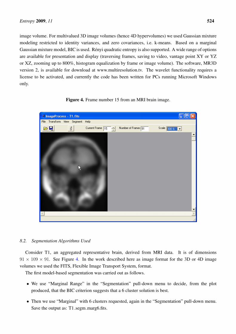
image volume. For multivalued 3D image volumes (hence 4D hypervolumes) we used Gaussian mixturemodeling restricted to identity variances, and zero covariances, i.e. k-means. Based on a marginalGaussian mixture model, BIC is used. Renyi quadratic entropy is also supported. A wide range of optionsare available for presentation and display (traversing frames, saving to video, vantage point XY or YZor XZ, zooming up to 800%, histogram equalization by frame or image volume). The software, MR3Dversion 2, is available for download at www.multiresolution.tv. The wavelet functionality requires alicense to be activated, and currently the code has been written for PCs running Microsoft Windowsonly.

Figure 4. Frame number 15 from an MRI brain image.

8.2. Segmentation Algorithms Used

Consider T1, an aggregated representative brain, derived from MRI data. It is of dimensions91 × 109 × 91. See Figure 4. In the work described here as image format for the 3D or 4D imagevolumes we used the FITS, Flexible Image Transport System, format.

The first model-based segmentation was carried out as follows.

• We use “Marginal Range” in the “Segmentation” pull-down menu to decide, from the plotproduced, that the BIC criterion suggests that a 6 cluster solution is best.

• Then we use “Marginal” with 6 clusters requested, again in the “Segmentation” pull-down menu.Save the output as: T1 segm marg6.fits.

Entropy 2009, 11 525

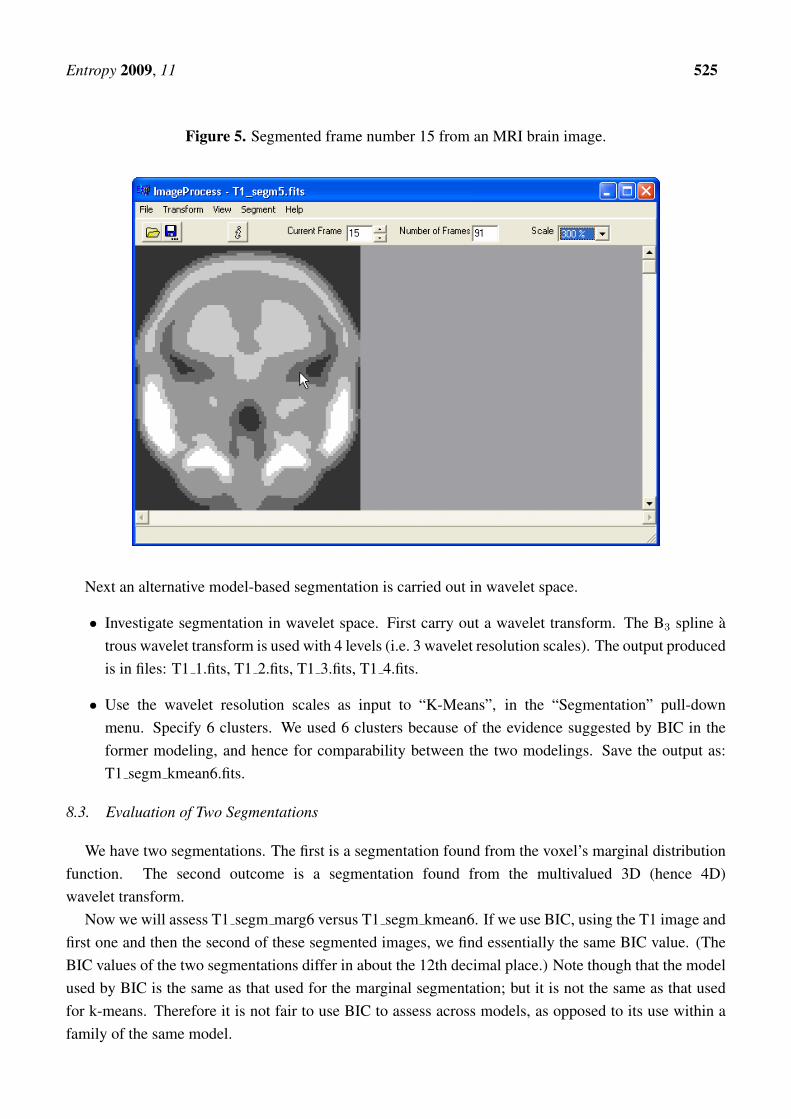
Figure 5. Segmented frame number 15 from an MRI brain image.

Next an alternative model-based segmentation is carried out in wavelet space.

• Investigate segmentation in wavelet space. First carry out a wavelet transform. The B3 spline atrous wavelet transform is used with 4 levels (i.e. 3 wavelet resolution scales). The output producedis in files: T1 1.fits, T1 2.fits, T1 3.fits, T1 4.fits.

• Use the wavelet resolution scales as input to “K-Means”, in the “Segmentation” pull-downmenu. Specify 6 clusters. We used 6 clusters because of the evidence suggested by BIC in theformer modeling, and hence for comparability between the two modelings. Save the output as:T1 segm kmean6.fits.

8.3. Evaluation of Two Segmentations

We have two segmentations. The first is a segmentation found from the voxel’s marginal distributionfunction. The second outcome is a segmentation found from the multivalued 3D (hence 4D)wavelet transform.

Now we will assess T1 segm marg6 versus T1 segm kmean6. If we use BIC, using the T1 image andfirst one and then the second of these segmented images, we find essentially the same BIC value. (TheBIC values of the two segmentations differ in about the 12th decimal place.) Note though that the modelused by BIC is the same as that used for the marginal segmentation; but it is not the same as that usedfor k-means. Therefore it is not fair to use BIC to assess across models, as opposed to its use within afamily of the same model.

Entropy 2009, 11 526

Using Renyi quadratic entropy, in the “Segmentation” pull-down menu, we find 4.4671 for themarginal result, and 1.7559 for the k-means result.

Given that parsimony is associated with small entropy here, this result points to the benefits ofsegmentation in the wavelet domain, i.e. the second of our two modeling outcomes.

9. Conclusions

We have shown that Renyi quadratic entropy provides an effective way to compare model families. Itbypasses the limits of intra-family comparison, such as is offered by BIC.

We have offered some preliminary experimental evidence too that direct unsupervised classificationin wavelet transform space can be more effective than model-based clustering of derived data. Intendedby the latter (“derived data”) are marginal distributions.

Our innovative results are very efficient from computational and storage viewpoints. The wavelettransform for a fixed number of resolution scales is computationally linear in the cardinality of the inputvoxel set. The pairwise interaction terms feeding the Renyi quadratic entropy are also efficient. For bothof these aspects of our work, iterative or other optimization is not called for.

Acknowledgements

Dimitrios Zervas wrote the graphical user interface and contributed to other parts of the softwaredescribed in Section 8.

References

1. McCullagh, P. What is a statistical model? Ann. Statist. 2002, 30, 1225–1310.2. Djorgovski, S.G.; Mahabal, A.; Brunner, R.; Williams, R.; Granat, R.; Curkendall, D.; Jacob, J.;

Stolorz, P. Exploration of parameter spaces in a Virtual Observatory. Astronomical Data Analysis2001, 4477, 43–52.

3. Silk, J. An astronomer’s perspective on SCMA III. In Statistical Challenges in Modern Astronomy;Feigelson, E.D., Babu, G.J., Eds.; Springer: Berlin, Germany, 2003; pp. 387–394.

4. Nagy, G. State of the art in pattern recognition. Proc. IEEE 1968, 56, 836–862.5. Murtagh, F.; Raftery, A.E.; Starck, J.L. Bayesian inference for multiband image segmentation via

model-based cluster trees. Image Vision Comput. 2005, 23, 587–596.6. Rissanen, J. Information and Complexity in Statistical Modeling; Springer: New York, NY, USA,

2007.7. Hansen, M.H.; Bin, Y. Model selection and the principle of minimum description length. J. Amer.

Statist. Assn. 2001, 96, 746–774.8. Fraley, C.; Raftery, A.E. How many clusters? Which clustering method? – answers via

model-based cluster analysis. Comput. J. 1998, 41, 578–588.9. Blum, R.S.; Zhang, Y.; Sadler, B.M.; Kozick, R.J. On the approximation of correlated

non-Gaussian noise PDFs using Gaussian mixture models; Conference on the Applications ofHeavy Tailed Distributions in Economics, Engineering and Statistics; American University:Washington, DC, USA, 1999.

Entropy 2009, 11 527

10. Wang, S.; Zhao, Y. Online Bayesian tree-structured transformation of HMMs with optimal modelselection for speaker adaptation. IEEE Trans. Speech Audio Proc. 2001, 9, 663–677.

11. Murtagh, F.; Starck, J.L. Quantization from Bayes factors with application to multilevelthresholding. Pattern Recognition Lett. 2003, 24, 2001–2007.

12. Murtagh, F.; Starck, J.L. Bayes factors for edge detection from wavelet product spaces. Opt. Eng.2003, 42, 1375–1382.

13. Principe, J.C.; Xu, D.X. Information-theoretic learning using Renyi’s quadratic entropy;International Conference on ICA and Signal Separation; Aussios, France, August 1999; pp.245–250.

14. Esteban, M.D.; Morales, D. A summary of entropy statistics. Kybernetika 1995, 31, 337–346.15. Cachin, C. Entropy Measures and Unconditional Security in Cryptography, Ph.D. Thesis, ETH

Zurich: Zurich, Switzerland, 1997.16. Starck, J.L.; Murtagh, F. Astronomical Image and Data Analysis; Springer: Berlin, Germany, 2002.

2nd ed., 2006.17. Starck, J.L.; Murtagh, F.; Fadili, J. Sparse Image and Signal Processing: Wavelets, Curvelets,

Morphological Diversity; Cambridge University Press: Cambridge, UK (forthcoming).18. Murtagh, F.; Starck, J.L.; Berry, M. Overcoming the curse of dimensionality in clustering by means

of the wavelet transform. Comput. J. 2000, 43, 107–120.19. Murtagh, F.; Starck, J.L. Pattern clustering based on noise modeling in wavelet space. Pattern

Recognition Lett. 1998, 31, 847–855.20. Starck, J.L.; Murtagh, F.; Gastaud, R. A new entropy measure based on the wavelet transform

and noise modeling. IEEE Transactions on Circuits and Systems – II: Analog and Digital SignalProcessing 1998, 45, 1118–1124.

21. Shannon, C.E. A mathematical theory for communication. Bell Systems Technical Journal 1948,27, 379–423.

22. Frieden, B. Probability, Statistical Optics, and Data Testing: A Problem Solving Approach; 2nded.; Springer-Verlag: New York, NY, USA, 1991.

23. Burg, J. Multichannel maximum entropy spectral analysis, Multichannel Maximum EntropySpectral Analysis; Annual Meeting International Society Exploratory Geophysics, reprinted inModern Spectral Analysis; Childers, D.G., Ed.; IEEE Press: Piscataway, NJ, USA, 1978; pp.34–41.

24. Frieden, B. Image enhancement and restoration; In Topics in Applied Physics; Springer-Verlag:Berlin, Germany, 1975; Vol. 6, pp. 177–249.

25. Gull, S.; Skilling, J. MEMSYS5 Quantified Maximum Entropy User’s Manual; Maximum EntropyData Consultants: Cambridge, UK, 1991.

26. Gokcay, E.; Principe, J.C. Information theoretic clustering. IEEE Trans. Patt. Anal. Mach. Int.2002, 24, 158–171.

27. MacKay, D.J.C. Information Theory, Inference, and Learning Theory; Cambridge University Press:Cambridge, UK, 2003.

28. Lee, Y.J.; Choi, S.J. Minimum entropy, k-means, spectral clustering, In Proceedings of theInternational Joint Conference on Neural Networks (IJCNN); Budapest, Hungary, July 25–29,

Entropy 2009, 11 528

2004; pp. 117–122.29. Jenssen, R. Information theoretic learning and kernel methods; In Information Theory and

Statistical Learning; Emmert-Streib, F., Dehmer, M., Eds.; Springer: New York, NY, USA, 2009.30. Katz, J.O.; Rohlf, F.J. Function-point cluster analysis. Syst. Zool. 1973, 22, 295–301.31. Murtagh, F. A survey of algorithms for contiguity-constrained clustering and related problems.

Comput. J. 1985, 28, 82–88.

c© 2009 by the authors; licensee Molecular Diversity Preservation International, Basel, Switzerland.This article is an open-access article distributed under the terms and conditions of the Creative CommonsAttribution license http://creativecommons.org/licenses/by/3.0/.