20-l

Gamma Mixture Models for Target Recognition

Andrew R. Webb

Defence Evaluation and Research Agency, St Andrews Road,

Malvern, Worcestershire WR14 3PS.

E-mail: webb@signal . dera . gov . uk

1. SUMMARY

This paper considers a mixture model approach to automatic target recognition using high resolution radar measurements. The mixture model approach is motivated from several perspectives including re- quirements that the target classifier is robust to am- plitude scaling, rotation and transformation of the target.

Latent variable models are considered as a means of modelling target density. These provide an ex- plicit means of modelling the dependence on angle of view of the radar return. This dependence may be modelled using a nonlinear transformation such as a radial basis function network.

A more simple model with separate components is considered. Estimation of the model parameters is achieved using the expectation-maximisation (EM) algorithm. Gamma mixtures are introduced and the EM re-estimation equations derived. These mod- els are applied to the classification of high resolution radar range profiles of ships (where results are com- pared with a previously-published self-organising map approach) and ISAR images of vehicles.

2. INTRODUCTION

This paper develops work in [16] and addresses the problem of automatic target recognition using mix- ture models of radar target density and applies these models to the classification of radar range profiles of ships and ISAR images of vehicles. Our aim is to obtain an estimate of the posterior probability of class membership, p(j]s), for class j and measure- ment vector z. We seek to achieve this via Bayes theorem,

PWE) = P(Zlj)P(j)

C P(4Mj) (1)

where p(x lj) are the class-conditional densities and p(j) are the class priors. The reason why we seek di- rect estimates of p(jlx) rather than to design a clas- sifier with class decisions as the output (for example,

a nearest neighbour classifier) is that the classifier will in general form part of a hierarchical decision making process. Classification is not an end in itself and will lead to some actions. Cost of making deci- sions will need to be considered. Also, supplementary domain-specific information (such as intelligence re- ports) may need to be combined with sensor-derived results in the decision making process. Therefore it is important that a classifier gives some measure of con- fidence that a pattern belongs to a particular class. This is provided by the probability of class member- ship.

The most common measure of the performance of a classification rule is misclassification rate or error rate. Error rate suffers from several disadvantages [17]. Error rate is deficient in that it treats all mis- classifications equally and does not distinguish be- tween p(j15) = 1 and p(jlx) = 0.51, which for a two-class case results in the same classification; that is, it does not distinguish between estimates of the probabilities of class membership that are close to the threshold of 0.5 and those far from 0.5. Also, error rate does not distinguish between a rule that is bad because classes heavily overlap in data space or a rule that is bad because probabilities of class mem- bership are poorly estimated. Discussion of classifier performance assessment is beyond the scope of the current paper and has been treated elsewhere [17].

However, estimation of the posterior probabilities, p(jlx), through estimation of the class-conditional densities, p(x/ j) and Bayes theorem (1) is not with- out its difficulties. The main difficulty is in the es- timation of target densities for data lying in a high- dimensional space. For the range profile data consid- ered later in this paper, the data vectors xi lie in a 130-dimensional space (xi E IR13’) and nonparamet- ric methods of density estimation (for example, ker- nel methods) are impractical due to the unrealistic amounts of data required for accurate density esti- mation. An alternative approach is to trade flexibil- ity for robustness and to use some simple parametric forms for the densities (for example, normal distri- butions) for which good estimates of the parameters may be obtained. Yet these may impose too much

Paper presented at the RTO SCI Symposium on ‘Non-Cooperative Air Target Identification Using Radar”, held in Mannheim, Germany, 22-24 April 1998, and published in RTO MP-6.

20-2

rigidity on the allowable forms of the density. The variance in the estimates of the parameters

of a simple model may be lower than that of a more complex model, but it would be expected to yield biased probability estimates for much of the z space. However, if simple classification is the main aim, then bias may not’ be relevant: the best achiev- able classification results will be obtained provided I;(~]z) > fi(j]~) whenever p(i]z) > p(j]z) (see, for example, [7]).

Alternatively, we may estimate the posterior prob- abilities of class membership directly through a dis- criminative function approach such as a neural net- work. These models provide approximations asymp- totically to the probabilities of class membership [9]. However, the amount of data required is excessive for high-dimensional data problems. There are several ways to circumvent this problem including linear pro- jections (such as principal components analysis) and nonlinear projections [14, 151 to a lower dimensional subspace.

The approach considered in this paper is to model the density as a mixture of simple parametric forms whose parameters are estimated through some opti- misation procedure. The advantage of such an ap- proach, as we see in Section 3, is that it may be used to incorporate desirable features such as robustness to translation of a test image with respect to some centroid position (due to uncertainty in the true cen- troid) and robustness to scale. Further, angular de- pendence of the target return can naturally be ex- pressed as a mixture, and different scattering models may also be incorporated into the same framework.

The basic distribution that we use at the heart of our model is a gamma distribution whose use may be motivated from physical arguments and results of empirical investigations.

The outline of the paper is as follows. Section 3 describes the mixture model approach to target clas- sification and how robustness of the model may be incorporated into the mixture model framework. A nonlinear latent variable models for density estima- tion is introduced as a means of modelling target den- sity (section 3.1) and a special case of independent mixture components considered. Section 4 derives the re-estimation procedure for the mixture model parameters. Section 5 presents results of applying the basic mixture model approach to the classifica- tion of radar range profiles; section 6 presents results of applying the approach to ISAR image data. The paper concludes with a summary of the main results and discussion of ways forward.

3. MIXTURE MODELS

In constructing the target probability density function, we wish to exploit expected structure in the data, without making assumptions that are too re- strictive or unrealistic, such as normal distributions.

We do this through mixture distributions. We shall assume that data are gathered on each

of C target types as a function of aspect angle. For simplicity, we assume a single angle coordinate (data gathered as a function of azimuth at a fixed elevation) although in principle azimuth and elevation may be considered. The data comprise radar cross section range profiles and a set of d measurements corre- sponding to d range gates encompassing the target is extracted’. Thus, for each class, j, the training data set is {zi,i = 1,. . ., Nj ; pi E lRd}, where Nj is the number of patterns in class j. The zi are usually ordered by angle. On test, we cannot assume that we know the physical position of the target precisely. Therefore, we must have a strategy for extracting an appropriate set of d range gate measurements from the range profile.

We start from the premise that we wish to model the probability density function of the target return, Pan c = 1,. . (C, where 2 is a set of target mea- surements. We choose to model this density as a fi- nite mixture [6, 131. Mixture models have been used with success in a wide variety of applications and here we consider their application to radar target mod- elling. We motivate their use by addressing, in turn, several important issues concerning the properties of the probability density function. We drop the suffix c since we are not concerned with a specific class.

3.1 Latent Variable Model

We assume that the distribution of radar returns is characterised by a latent variable 8,

where Q(t9) are parameters characterising the distri- bution and are functions of the variable 0. In the case of the gamma distribution (discussed in section 3.6), they are the mean and the order parameters. For the radar target data, 8 is univariate and can be interpreted as .angle.

Figure 1 illustrates the basic model. The latent space is represented by an angle 8. This is mapped to a parameter space, Q(e), by a nonlinear model (for example, a radial basis function network (RBF)). Data is generated according to the probability distri- bution p(5]8). In the data space, the data can be viewed as perturbations from a closed-loop contour.

If we suppose that Q(e) does not vary too rapidly with 8, then we may approximate the integral above by a finite sum,

p(5) = &m%)) (2) i=l

‘For the ISAR data, the d measurements correspond to the d cells in the ISAR image. However, the discussion in this section is confined to radar range profiles.

20-3

or in matrix form

Xl

Figure 1. Latent

RBF

variable model.

where the 8i are samples on a regular grid. Equa- tion (2) is a finite mixture distribution and the prob- lem of calculating p(z) is replaced by one of calcu- lating, or specifying, the component distributions, ~(zP(h)), the P arameters associated these distri- butions, and the component distribution weights, pi. Given a data set, and some simple parametric form for each of the p( z ] @ (Oi)) ) a maximum likelihood ap- proach, perhaps based on the EM algorithm, may be employed.

Here, we shall regard the variable 8 as angle of view of the target. This may be a multivariate quan- tity comprising azimuth and elevation, but in the ex- amples of section 5, we consider azimuth only. Thus, Equation (7) states that for a given angle of look, 8, the target return, 5, is a sample from a distribution, p(~]e), and the total distribution is an integral over all angles of look.

For the gamma mixture model, there are two sets of parameters: the component means, p and the or- der parameters, m (both E IR”). For g components, we wish to re-estimate {ml,, lc = 1, . , g} and the means, {pk, lc = 1,. . , g}, which we regard as func- tions of underlying variables, 8 (in the ship and ve- hicle data 8 is univariate),

i=l

h (3) m = m(e) = Csidj(e)

i=l

where ~$i is a set of h specified basis functions (for example, radial basis functions) defined on the space characterised by 19 and {vi, i = 1, . , h} and {sd, i = 1, , h} are sets of weights to be determined.

The means and order parameters of the Icth group are

h

elk = Ovid%

u = V@

M = SG

where V = [vi] . ]vh], S = [si] . IshI and 0 = [+(&)I.. ]4(f3,)] and +(ek) is the h-dimensional vector with ith component +i(&). Thus, the pa- rameters of each component, & and mk, depend on the same set of underlying parameters, V and S.

The distribution, P(Z), may now be regarded as depending on two sets of vectors that characterise the means and order parameters: the d x h matrices V and S,

P(Z) = P(ZlS! v> Given a data set {pi, i = 1, n}, we seek to max-

imise the log likelihood

L = eln[p(zj]S, V)] j=l

with respect to the parameters of the model S and V. We shall not present the details of parameter estimation for latent variable models here, but note that

1.

2.

3.

4.

3.i

A radial basis function provides a flexible model for the nonlinear transformation from latent space to data space.

An EM scheme may be derived for the model parameters, but unless simplifications are made, the update equations for the means and order parameters are coupled, thus re- quiring some nonlinear optimisation scheme for their solution.

For normal mixtures, Bishop et al [l, 21 have derived EM update equations.

Smoothness may be ensured through incorpo- ration of a suitable prior on the models.

Using Angular Information

Knowledge of the angle at which measurements are made is not necessary as part of the latent vari- able model, but if it is available, how would we use it during training and test? During training, we would use 19i as part of the maximum likelihood re- estimation. Suppose that the training data comprise radar range profile (or ISAR) measurements together with the angle of look. Thus, we are given the data +, ej), i = 1,. . ) n}. We may write the joint dis- tribution as

p(~, 0) = d4ew (4

where the conditional density p(z 10) depends on pa- rameters that describe the density. If we assume a

20-4

gamma mixture with mean and order parameters be- ing a nonlinear function of angle, then

P(Zl@) = P(Sl@, S,V)

The log likelihood, L, is given by

L = 2 In {p(zal& I S, V)p(ei)> i=l

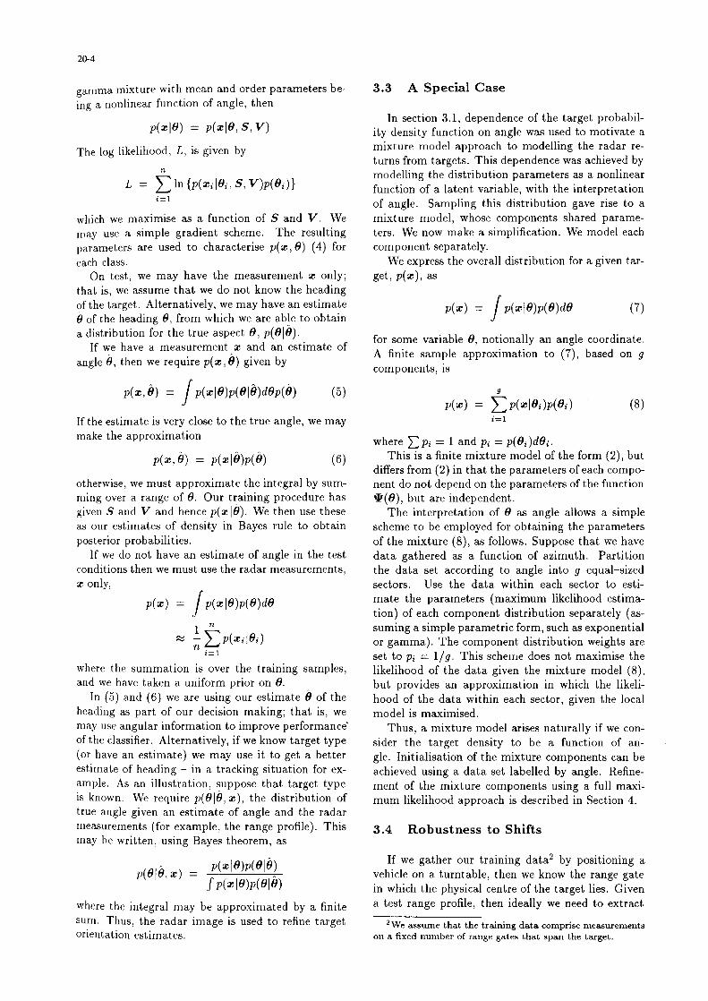
which we maximise as a function of S and V. We may use a simple gradient scheme. The resulting parameters are used to characterise p(z, 0) (4) for each class.

On test, we may have the measurement z only; that is, we assume that we do not know the heading of the target. Alternatively, we may have an estimate fi of the heading 8, from which we are able to obtain a distribution for the true aspect 8, ~(018).

If we have a measurement z and an estimate of angle 6, then we require p(z, h) given by

P(d) = J Pww@Wh@) (5)

If the estimate is very close to the true angle, we may make the approximation

P(T 4) = P(d@P@) (6)

otherwise, we must approximate the integral by sum- ming over a range of 8. Our training procedure has given S and V and hence p(z 14). We then use these as our estimates of density in Bayes rule to obtain posterior probabilities.

If we do not have an estimate of angle in the test conditions then we must use the radar measurements, 5 only,

P(X) = J Pbwdwe

where the summation is over the training samples, and we have taken a uniform prior on 8.

In (5) and (6) we are using our estimate fi of the heading as part of our decision making; that is, we may use angular information to improve performance’ of the classifier. Alternatively, if we know target type (or have an estimate) we may use it to get a better estimate of heading - in a tracking situation for ex- ample. As an illustration, suppose that target type is known, We require p(fIl8, z), the distribution of true angle given an estimate of angle and the radar measurements (for example, the range profile). This may be written, using Bayes theorem, as

ieW4 = P(e9P(e9 s dx m(eifi)

where the integral may be approximated by a finite sum. Thus, the radar image is used to refine target orientation estimates.

3.3 A Special Case

In section 3.1, dependence of the target probabil- ity density function on angle was used to motivate a mixture model approach to modelling the radar re- turns from targets. This dependence was achieved by modelling the distribution parameters as a nonlinear function of a latent variable, with the interpretation of angle. Sampling this distribution gave rise to a mixture model, whose components shared parame- ters. We now make a simplification. We model each component separately.

We express the overall distribution for a given tar- get, P(Z), a.3

for some variable 8, notionally an angle coordinate. A finite sample approximation to (7), based on g components, is

P(Z) = ~p(de)p(w i=l

where Cpi = 1 and pi = p(&)d&. This is a finite mixture model of the

(8)

form (2), but differs from (2) in that the parameters of each compo- nent do not depend on the parameters of the function *(e), but are independent.

The interpretation of 8 as angle allows a simple scheme to be employed for obtaining the parameters of the mixture (8), as follows. Suppose that we have data gathered as a function of azimuth. Partition the data set according to angle into g equal-sized sectors. Use the data within each sector to esti- mate the parameters (maximum likelihood estima- tion) of each component distribution separately (as- suming a simple parametric form, such as exponential or gamma). The component distribution weights are set to pi = l/g. This scheme does not maximise the likelihood of the data given the mixture model (8), but provides an approximation in which the likeli- hood of the data within each sector, given the local model is maximised.

Thus, a mixture model arises naturally if we con- sider the target density to be a function of an- gle. Initialisation of the mixture components can be achieved using a data set labelled by angle. Refine- ment of the mixture components using a full maxi- mum likelihood approach is described in Section 4.

3.4 Robustness to Shifts

If we gather our training data2 by positioning a vehicle on a turntable, then we know the range gate in which the physical centre of the target lies. Given a test range profile, then ideally we need to extract

‘We assume that the training data comprise measurements on a fixed number of range gates that span the target.

20-S

the test image z so that the centre of the target lies in the same range gate. We then evaluate p(z) for each class. However, in practice, we do not know the physical centre of the target (we may not know it for the training data if the target translates as it rotates ~ see Section 5), but we can calculate a centroid using the test range profile. We then need to extract d range gates around this centroid by deciding which range gate (1 to d) to position the centroid in.

Consider a single component of the mixture, p(~]ei). Suppose that we generate data from this component by random sampling. For each sample generated calculate its centroid. The centroid posi- tions will not necessarily be in the same range gate as the centroid of the distribution mean. There will be a distribution, p(s,), of centroid positions, s, E {l,...,d}.

We may partition the distribution, p(~]ei), ac- cording to the centroids of the generated data,

8”

where p(z JBi, s,) is the probability distribution of samples whose centroids are in cell s,

The quantity pi(s,) is the probability that the cen- troid occurs in s, from data generated by p(z]ei). It is determined by the distribution, p(~]ei) and may be estimated from that distribution through Monte Carlo simulation, by generating data and noting the distribution of centroid positions. The probabilities, pi(s,), depend on i, the mixture component.

Therefore, the overall target distribution may be written as the mixture,

~(4 = 2~~ 2 Pi(sn)P(4ej,sn) (10) i=l s,=l

To evaluate the above equation for a test sample Z, we may position the centroid of z over each allow- able centroid position (that is, each possible centroid position permitted by the distributions, p(a]ed)) in turn, then

1. sum over centroid positions (many may not contribute since pi(s,) = 0, the centroid po- sition is not allowable for that component)

2. sum over components

Thus, we have expressed the robustness to pattern translation problem as a mixture formulation (Equa- tions (9) and (10)). In theory, the particular algo- rithm used to calculate the centroid position is unim- portant. Although the distribution of centroid posi- tions depends on this algorithm, we integrate over all possible centroid positions. In practice, however, it may be preferable to have an estimate of centroid po- sition with a narrow distribution, pi(s,). This would reduce computational costs since for many values of s,, pi(s,) = 0 - samples with that centroid do not occur for p(zlei).

3.5 Robustness to Amplitude Variation

We may need to scale the test image to normalise the data (the test samples may be measured at a dif- ferent signal-to-noise ratio that the training data). In the above analysis, we partitioned the data gener- ated by a component according to the centroid posi- tion. We may also partition according to the overall amplitude level of the test pattern. Let A denote some overall amplitude measurement of a pattern.

dew = ~pw4,-4~d4 A

where p( z lOi, A) is the probability distribution of samples whose overall amplitude is A, assumed to take discrete values.

To evaluate for a given Z, we scale it to have am- plitude A and substitute into

p(z) = epi ~p(zl&,Ah(A) i=l A

Thus, in a similar manner to robustness to shifts, we can treat robustness to amplitude scaling by formu- lating a mixture model.

For computational convenience, we need to dis- cretize A. Also, we need to define a scheme for cal- culating the amplitude of a pattern. As in the cen- troid situation, in principle it does not matter how we calculate A, given 5, since we integrate over the distribution of A. In practice, it may be important. If our estimator of amplitude has a narrow distribu- tion, then we could take the one extreme that the amplitude distribution is approximated by one cell at the distribution mean. Thus, all test images are scaled to the distribution mean.

3.6 Target Distribution

We still need to specify the forms of the mixture component distributions. For example, we may again take an exponential distribution, although gamma distributions may be more appropriate. The gamma distribution

dx) = (mml)!p p (!E)m-lexp (-7)

has as special cases the Swerling 1 and 2 models (m = 1, Rayleigh statistics), Swerling 3 and 4 (m = 2) and the non-fluctuating target (m + 03), although other values of m have been observed empirically [la].

A simple multivariate form is to assume indepen- dence of range gates so that the component distribu- tion is given by

Pwu = I f

mij

( )

mij m , , - 1

j=l (mij - l)!pij X

pij

??lij 2 exp --

( > Pij

20-6

where m,j is the order parameter for range gate j of component i and pij is the mean.

We may of course represent the component distri- bution itself as a mixture in order to model different scattering distributions. Further, we may partition it into two basic components,

P(XPi) = Pd(X) + Pn4X) (11)

where t(z) is a target distribution, n(z) a noise or clutter distribution and pt and p, are prior probabil- it,ies (pl + p, = 1). This allows the presence of noise to be t.aken into account.

3.7 Summary

In this section we have described several different ways in which mixture models may arise in a target modelling situation.

1. to incorporate angular dependencies.

2. to ensure robustness to uncertainty in target centroid position.

3. to ensure robustness to overall amplitude vari- ation.

4. to model different types of target behaviour

5. to incorporate both noise and target models to reduce sensitivity to noise on test.

The advantage of the mixture model approach is that it provides a simple flexible model for the dis- tribution of target returns, while also incorporating into the same framework features such as robustness that are important in a practical implementation.

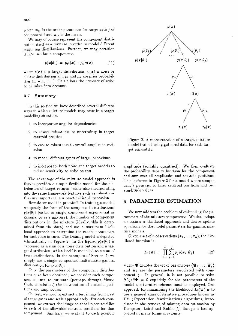
How do we use it in practice? In training a model, we specify the form of the component distributions, p(zl0i) (either as single component exponential or gamma, or as a mixture), the number of component distributions in the mixture (ideally, this is deter- mined from the data) and use a maximum likeli- hood approach to determine the model parametefs for each class in turn. The training model is depicted schematically in Figure 2. In the figure, ~(~18;) is expressed as a sum of a noise distribution and a tar- get distribution, which itself is modelled as a sum of two distributions. In the examples of Section 5, we simply use a single component multivariate gamma distribution for p(zlea).

Once the parameters of the component distribu- tions have been obtained, we consider each compo- nent in turn to estimate (perhaps through Monte Carlo simulat,ion) the distribution of centroid posi- tions and amplitudes.

On test, we need to extract a test image from a set of range gates and scale appropriately. For each com- ponent’, we ext,ract the image so that its centroid lies in each of the allowable centroid positions for that component,. Similarly, we scale it to each possible

P(X)

A PC@1 1 PCei> (0,)

. . .

A Pn Pt

n(x) t(x)

Pt1

A

Pt2

t1 (x) tdx)

Figure 2. A representation of a target mixture model trained using gathered data for each tar- get separately.

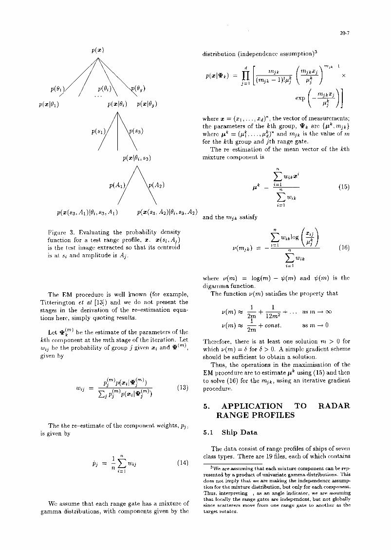
amplitude (suitably quantised). We then evaluate the probability density function for the component and sum over all amplitudes and centroid positions. This is shown in Figure 3 for a model where compo- nent i gives rise to three centroid positions and two amplitude values.

4. PARAMETER ESTIMATION

We now address the problem of estimating the pa- rameters of the mixture components. We shall adopt a maximum likelihood approach and derive update equations for the model parameters for gamma mix- ture models.

Given a set of n observations (x1, . , xn), the like- lihood function is

i=l j=l

where @ denotes the set of parameters { %@I, . . . , !Pg} and Qj are the parameters associated with com- ponent j. In general, it is not possible to solve dLo/d* = 0 explicitly for the parameters of the model and iterative schemes must be employed. One approach for maximising the likelihood Lo(Q) is to use a general class of iterative procedures known as EM (Expectation-Maximisation) algorithms, intro- duced in the context of missing data estimation by Dempster, Laird and Rubin [5], though it had ap- peared in many forms previously.

P(X)

A de1 > P(h) (fJ,>

. . .

P(ZPl) P(XPi) PGW

P(Sl)

A

(s3)

P(Zl&, $3)

distribution (independence assumption)3

p(xl*k) = fi j=l [ (&y)!$; (yy”’ x

wherez = (zr,...,zd)*, the vector of measurements; the parameters of the kth group, IPk are {pkrmjk} where pk = (/I!, . , &)* and mjk is the value of m for the kth group and jth range gate.

The re-estimation of the mean vector of the kth mixture component is

n

c WikXi

k _ i=l P- n

c Wik

i=l

(15)

~(4~3, Al)Pi, ~3, Al) P(X(S3, AM, S3,A2) and the mjk satisfy

Figure 3. Evaluating the probability density function for a test range profile, 2. z(si, Aj) is the test image extracted so that its centroid is at si and amplitude is Aj.

The EM procedure is well known (for example, Titterington et al [13]) and we do not present the stages in the derivation of the re-estimation equa- tions here, simply quoting results.

Let KP(kn) be the estimate of the parameters of the kth component at the mth stage of the iteration. Let wij be the probability of group j given zi and QCrn), given by

p!m)p(Xi I*‘“‘) Wdj =

3 3 cj p,!“‘p( zi IQ;“‘)

(13)

The the re-estimate of the component weights, pj, is given by

?;j = $ g wij (14) t=l

We assume that each range gate has a mixture of gamma distributions, with components given by the

k c$ wiklog

v(mjk) = - ‘=’ n ( ) 3

(16)

c Wik i=l

where v(m) = log(m) - $(m) and ti(m) is the digamma function.

The function v(m) satisfies the property that

v(m) x Sk+

A+... asm+cx

v(m) % & + const. asm-0

Therefore, there is at least one solution m > 0 for which v(m) = b for 6 > 0. A simple gradient scheme should be sufficient to obtain a solution.

Thus, the operations in the maximisation of the EM procedure are to estimate pk using (15) and then to solve (16) for the mjk, using an iterative gradient procedure.

5. APPLICATION TO RADAR RANGE PROFILES

5.1 Ship Data

The data consist of range profiles of ships of seven class types. There are 19 files, each of which contains

3 We are assuming that each mixture component can be rep- resented by a product of univariate gamma distributions. This does not imply that we are making the independence assump tion for the mixture distribution, but only for each component. Thus, interpreting i as an angle indicator, we are assuming that locally the range gates are independent, but not globally since scatterers move from one range gate to another as the target rotates.

20-8

range profiles of a ship which are recorded as the ship turns through 360 degrees. The aspect angle of the ship varies smoothly as one steps through the file and the centroid of the ship drifts across range gates as the ship turns. Each range profile consists of 130 measurements on radar returns from 130 range gates. These data sets have been used by Luttrell [lo] and d&ails are given in Table 1. The data sets are divided

Target Class

1

no of profiles Train Test

3334 I 2085 2 2636,4128 2116 3 2604, 2248, 2923 2476, 3619 4 8879, 3516 4966, 2560 5 3872 3643 6 1696 2216 7 1839

Table 1. Details of data files

into 11 training files and 8 test files. As we can see from the table, there is no test data available for class 7. Several other classes have more than one rotation available for training and testing.

Iq each of the experiments below, 1200 samples over 360 degrees from each of the training set files were used in model training. This enables compari- son to be made with the results of Luttrell [lo].

5.2 Implementation Details

In each experiment, a mixture model density was constructed (using the basic approach described in section 3) for each file and those densit,ies correspond- ing to the same target type are combined with equal weight. For a mixture model with g components, the parameters of the mixture model were initialised by dividing the data into g equal angle sectors and for each sector separately calculating the maximum like- lihood estimate of the mean and order parameters of the gamma distribution. The EM algorithm was run on the whole training data set and the final value of the log likelihood, log(L), at convergence recorded.,

There has been considerable research into model selection for multivariate mixtures. We adopted a simple approach and took our model selection crite- rion to be

AIC2 = -2log(L) + 2N,

where NP is the number of parameters in the model,

Np = 2(d + 1)g - 1

This has been considered by Bozdogan and Sclove [3]; other measures are described and assessed be Celeux and Soromenho [4].

Once the components of the mixture model have been determined, samples form the component dis- tributions were generated and the distribution of the

centroids measured for each mixture component. It was found that most samples (> 99%) lay within two range gates of the position of the centroid of the com- ponent mean. Therefore on test, a test pattern was shifted to all positions within 2 range gates of the component mean.

The amplitude of the test pattern was scaled to the amplitude of the component mean.

5.3 Ship Profiles

Below we give results of the method applied to the ship data. We report confusion matrices despite their limitations as measures of classifier performance. Ide- ally we would like to say how well the estimate of the posterior density, l;(jl~), approximates the true den- sity p(jlz). A measure of this discrepancy is the re- liability of the classifier [ll] or imprecision [8]. How- ever, p(jjz) is unkcown in practice and techniques for evaluating bounds .YL imprecision are currently under investigation.

5.3.1 Experiment 1

In this experiment, the classifier is trained with 40 components per file and tested on the test data files with the ship orientated so that it is in the range f40 degrees bow-on or stern-on to the radar. This restriction is applied so that the results may be com- pared with those given by Luttrell [lo], where a classi- fier based on a self-organising network was designed. Table 2 reproduces the results of Luttrell [lo] and gives the mixture model results alongside.

Predicted Class

Predicted Class

Table 2. Gamma mixture results (top) and self- organising network results (bottom) [lo] for a test set pattern &40 degrees bow-on or stern- on to the radar.

The average classification performance on test of the mixture model approach is 67.9% compared to 64.6% given by Luttrell [lo]. There are some notable differences in performance: there is much better clas-

20-9

sification rate on classes 1 and 2 and much poorer performance on class 6.

5.3.2 Experiment 2

In this experiment, mixture models were trained with varying numbers of components and tested on the whole of the test set (there is no angle restriction). Again, 1200 samples per file were used and Figure 4 plots the model selection criterion AIC2 as a function of the number of components for each of the training files. Figure 5 plots the classification rate as a func- tion of the number of components, where each model has the same number of components. The minimum of AIC2 occurs for each of the 11 files when the num- ber of components is given by (80, 80, 70, 70, 60, 80, 70, 70, 50, 70, 100). Thus, each model requires a different number of components. The classification performance for this model is given in table 3.

The overall classification rate is 64% for the se- lected model. This is about the level of the plateau region in Figure 5. Thus the AIC2 criterion has pro- vided a model that is close to the best test set per- formance over the range of model sizes considered.

Figure 4.. AIC2 as a function of the number of mixture components for each file in the training set.

Predicted Class

Table 3. Gamma mixture results for the whole test set for a model chosen according to mini- mum values of AIC2.

Figure 5. Classification rate as a function of the number of mixture components for the ship data.

6. APPLICATION TO ISAR IMAGES

6.1 Vehicle Data

The data comprise single polarisation TSAR im- ages of three vehicles measured on a turntable. There are two rotations of each vehicle. For each vehicle and each rotation, there are 2000 patterns. The im- age size is 16 x 20.

A third data set of ‘similar’ vehicles, but not the same measure type, was also considered as part of an experiment into classifier robustness - see the paper by Britton in these proceedings

6.2 Results

Results for the training set, the second rotation and the separate ‘test’ set (that differed in some de- tail from the training data) are given in Figure 6. Each data set was modelled using a gamma mixture model in which the means and order parameters were re-estimated. ‘Again, the criterion AC12 was used to control the complexity of the model. In terms of mod- elling the data on the second rotation, performance is still increasing at 70 components per class. The AIC2 measure has not reached a minimum at this point.

7. SUMMARY AND DISCUSSION

In this paper we have developed a gamma mixture model approach to the classification of radar range profiles and ISAR images. A latent variable model was introduced as one means of modelling the smooth variation of the underlying distribution with angle. EM update equations for the model parameters of a basic mixture model were derived. Robustness to amplitude scaling of the test pattern and unknown orientation and location of the target can be taken into account in the mixture model framework. The approach has been applied to the classification of ship

Figure 6. Classification rate as a function of the number of mixture components for the vehicle data.

profiles (giving improved performance, in terms of error rate, achieved compared with previously pub- lished results) and to ISAR images of vehicles.

However, error rate is only one measure of perfor- mance. It does not tell us how good t,he classifier is. We may get an error rate of 40% say, but if the classes are indeed separable (for the given features), then we could improve performance by better classi- fier design. Yet, if the Bayes error rate is itself 40%, then we are wasting effort trying to improve classifier design. We must seek additional variables or features. This is one of the motivations behind the work in this paper: to provide estimates of the posterior proba- bilities that may be combined with other information (for example, misclassification costs, domain-specific data, intelligence reports) in a hierarchical manner for decision making.

Thus, we have developed a semi-parametric den- sity estimator that incorporates robustness features and makes use of physical/empirical scattering dis- tributions. The approach may not give better per- formance in terms of error rate than some other clas- sifiers (although it is clearly better than single com- ponent parametric distributions), but hopefully bet- ter approximations to the true posterior probabili- ties. This is difficult to assess and remains an issue for continuing study. Initial work is reported by Yu et al [17]. Other areas for further work include further assessment on two-dimensional (SAR/ISAR) images, development of the latent variable models and sensi- tivity to noise and clutter.

References

[I] C. Bishop, M. Svenskn, and C. Williams. EM op-

timization of latent-variable density models. In D. Touretsky, M. Mozer, and M. Hasselmo, editors,

Advances in Neural Information Processing Systems 8, pages 465-471. MIT Press, 1996.

[2] C. Bishop, M. Svenskn, and C. Williams. GTM: a principled alternative to the self-organizing map. In M. Mozer, M. Jordan, and T. Petsche, editors,

[31

[41

[51

[61

PI

PI

PI

PO1

WI

WI

[I31

[I41

V51

I161

[ITI

Advances in Neural Information Processing Systems

9, pages 354-360. MIT Press, 1997. H. Bozdogan and S. Sclove. Multi-sample cluster analysis using Alaike’s information criterion. Annals

of Institute of Statistical Mathematics, 36:163-180, 1984.

G. Celeux and G. Soromenho. An entropy crite- rion for assessing the number of clusters in a mix- ture model. Journal of Classification, 13(2):195-212,

1996. A. Dempster, N. Laird, and D. Rubin. Maximum

likelihood from incomplete data via the EM algo- rithm. Journal of the Royal Statistical Society B,

39:1-38, 1977. B. Everitt and D. Hand. Finite Mixture Distribu-

tions. Monographs on Statistics and Applied Prob-

ability. Chapman and Hall, London, 1981. J. Friedman. On bias, variance, O/l loss, and the curse of dimensionality. Data Mining and Knowledge

Discovery, 1:55-77, 1996. D. Hand. Construction and Assessment of Classifi- cation Rules. John Wiley, Chichester, 1997. D. Lowe and A. Webb. Optimized feature extraction

and the bayes decision in feed-forward classifier net- works. IEEE Transactions on Pattern Analysis and

Machine Intelligence, 13(4):355-364, 1991. S. Luttrell. Using self-organising maps to classify

radar range profiles. In 4th International Confer- ence on Artificial Neural Networks, pages 335-340,

Cambridge, 1995. IEE, IEE. G. McLachlan. Discriminant Analysis and Statis-

tical Pattern Recognition. John Wiley, New York,

1992. M. Skolnik. Introduction to Radar Systems. McGraw-Hill Book Company, New York, second

edition, 1980. D. Titterington, A. Smith, and U. Makov. Statisti-

cal Analysis of Finite Mixture Distributions. John Wiley and Sons, New York, 1985.

A. Webb. Multidimensional scaling by iterative majorisation using radial basis functions. Pattern

Recognition, 28(5):753-759, 1995. A. Webb. An approach to nonlinear principal components analysis using radially-symmetric ker-

nel functions. Statistics and Computing, 6:159-168, 1996.

A. Webb. Gamma mixture models for target recog-

nition. 1997. (submitted for publication). K. Yu, D. Hand, and A. Webb. Evaluating the im- precision of classification rules. 1997. (submitted for

publication).

@British Crown Copyright 1998/DERA Published with the permission of the controller of

Her Britannic Majesty’s Stationery Office.