Acoustic Target Tracking and TargetIdentification - Recent Results1

Dr. George Succi, Torstein K. Pedersen,Robert Gampert and Dr. Gervaslo Prado

SenTech, Inc., Woburn, MA

IntroductionGround and air vehicles have distinctive acoustic signatures produced by theirengines and/or propulsion mechanism. The structure of these signatures makesthem amenable to classification by pattern recognition algorithms. There aresubstantial challenges in this process. Vehicle signatures are non-stationary byvirtue of variations in engine RPM and maneuvers. Field sensors are alsoexposed to substantial amounts of noise and interference. We discuss the use ofneural network techniques coupled with spatial tracking of the targets to carry outthe target identification process with a high degree of accuracy. Genericclassification is done with respect to the type of engine (number of cylinders) andspecific classification is done for certain types of vehicles. This paper will discussissues of neural network structure and training and ways to improve the reliabilityof the estimate through the integration of target tracking and classificationalgorithms.

The Acoustic Signature of VehiclesMilitary vehicles have loud and distinctive signatures. We focus on the use of lowfrequency noise components, because it is in this band that vehicles have theirstrongest emissions - also those components propagate with the leastattenuation. In the low end of the spectrum vehicles have two main sources ofsound: the engine and the propulsion gear (tires or tracks). Both of these sourcesoriginate with rotating components, thus they have a periodic characteristic.When viewed in the frequency domain, these periodic signals appear as familiesof harmonically related spectral lines (narrow band), Figure 1. Over time thefundamental frequency of these harmonic lines will change in concert withvariations in the engine RPM or the vehicle speed. Each type of engine, eachvehicle in many cases, has a signature with a particular pattern of harmonic linesin its spectrum. In order to identify a vehicle, our pattern recognition algorithmhas to be able to distinguish the essential invariant characteristics in this patternof harmonic lines. It is our goal to distinguish one vehicle from another by therelative amplitudes of the energy in the harmonics, what musicians call tonecolor. In most cases, this noise is from the periodic ignition of the fuel in thecylinders. The relative harmonic amplitude of the noise is influenced by thedetails of the engine design, the exhaust manifold, and the muffler. The noise

This work was funded by the Defense Advanced Research Projects Agency, Contract NumberDAAHOI -97-C-RI 95.

Part of the SPIE Conference on Unattended Ground Sensor Technologies and ApplicationsOrlando Florida • April 1999 SPIE Vol. 3713 • 0277-786X/99/$1O.OO

10

varies with vehicle velocity, engine rotation rate, source directivity, atmospherictransmission, and geometric attenuation

The Feature Extraction ProcessSome of these variations can be reduced by proper normalization. The effect ofengine speed can be removed by grouping the spectral lines according toharmonic number. The effect of distance can be (partially) removed by using therelative harmonic amplitude. When we make these corrections we are left with aseries of numbers, in the domain [0,1] - these are referred to as the feature setof this particular noise source, Figure 2. In the simplest model, these numbersrepresent the energy in the harmonics of the signal. Some components, like thefirst two harmonics are rarely seen clearly, so we exclude them from the set.The process of computing the harmonic line set starts with a short-term Fourieranalysis (FFT5). Spectral peaks are detected above a noise floor that iscomputed adaptively. Peaks are then sorted into harmonic sets. Each harmonicline set is treated as an "object" and is associated with a particular noise source.Targets can have more than one harmonic set: one for the engine and one forthe tracks for example.In addition to harmonic amplitude data, most sensors can measure the directionof arrival of the signal. This can be done in various ways, such as beamformingor phase comparison. Our sensors use very small aperture arrays, where the useof phase comparison is the most appropriate technique. A bearing can becomputed for each narrow band peak, and a combined bearing can be computedfor an entire harmonic set. Bearing estimation errors will depend on signal tonoise ratio and aperture size relative to the signal wavelength. With thisinformation, we can track the motion of each source in bearing vs. time space,creating a target track. A target track will connect all the measurementsassociated with a particular source while it remains detectable. Multiple targetscan be tracked simultaneously, as long as we can separate their spectralcomponents unambiguously. This allows us to track dissimilar targets such asairplanes and ground vehicles and even multiple ground vehicles. Figures 3 and4.

Pattern Recognition: Neural Networks vs. Statistical ClassifiersIn the simplest model of vehicle noise, the feature vector a is assumed to bedistributed about some mean value <a>. The spread of the vectors relative to thismean is described by the correlation matrix C. This correlation matrix representsan N dimensional surface that describes the statistical scatter in the data. If thedata has a multidimensional Gaussian distribution, these surfaces are ellipsoids.Choosing a probabilistic description for the feature data leads to a maximum-likelihood classification algorithm. In this approach, a feature vector can beclassified by computing the log-likelihood function that measures the likelihoodthe new vector belongs to one of the feature sets in our database. At this point,the Gaussian assumption becomes important, since it leads to a computationallyfeasible implementation. The problem is that the feature vectors are notdistributed randomly about a single value. We have found that in some vehicles

11

12

there are several mean values about which the data cluster depending on engineRPM and/or gear. To extend the simple model to accommodate the reality wewould have to construct a mean vector and correlation matrix for each of thedifferent operating conditions of the vehicle, Figure 5.Neural networks are well adapted to this complex mapping between the sourcefeature vector and the vehicle categories. A neural net is a mapping from thespace of the input vector to the space of the categories. The architecture of thenetwork is determined by the problem to be solved. The number of inputs is thesource feature vector a, the number of outputs is the number of categories wedefine. The number of layers between input and output and the sizes ofthe layerare up to the designer. Hidden layers handle the problem of disconnected orcomplex decision surfaces.One possible architecture is to use a single network with multiple outputs. Herewe use multiple networks with single outputs. There were two reasons for doingthis. The first was to make it easier to reconfigure the classifier to handle multipletargets. A neural network with multiple outputs will have to be retrained everytime we make a change to the target set. If each neural network represents onlyone target, then we do not need to retrain all networks when we make a change,Figure 6. The second reason has to do with the amount of computational effortneeded to re-train a neural network. It is much more efficient to train one neuralnetwork at a time.The two-layer sigmoid/linear network can represent any functional relationshipbetween inputs and outputs, if the sigmoid layer has enough neurons. We use atwo-layer network, i.e. a network with a single hidden layer. In our study wewished to place a vehicle in a particular category. In place of sigmoid/linear weused a sigmoid/sigmoid. The architecture is summarized as follows

0= f2(W2f1(Wia+bj)+b2)

Where the non-linear transfer function f operates on each element of the vector.The input is and Nxl vector, W1 is an N x N matrix, and b1 is an Nxl vector. Inour study we used one neural net for each category. The output o is a scalar, W2is a 1x12 matrix and b2 is a 12x I vector.In a typical sensor application, we maintain two neural networks. The first tries toclassify vehicles into specific categories - what we call vehicle identification. Thesecond network tries to classify the type of engine by the number of cylinders.The objective of this structure is twofold. First, the cylinder classifier will be ableto generalize better, since each engine category includes several types ofvehicles. The cylinder classifier can also be used to break ties, where the vehicleidentification net produces a tie between two dissimilar vehicles. Knowing theengine type gives the user some useful information about a vehicle even if it wasnot included in the training data.

Neural Network TrainingThe database is of moderate size. There are 18 vehicles, with 261 runs orpasses of two to three minutes in duration each, for a total of approximately

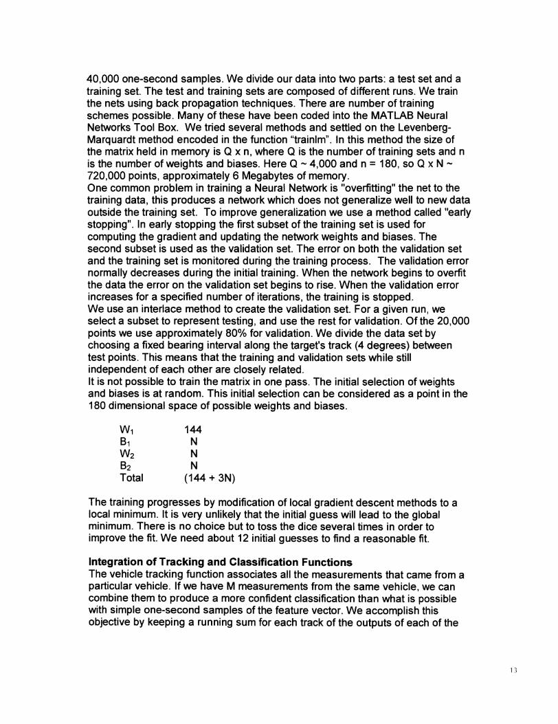
40,000 one-second samples. We divide our data into two parts: a test set and atraining set. The test and training sets are composed of different runs. We trainthe nets using back propagation techniques. There are number of trainingschemes possible. Many of these have been coded into the MATLAB NeuralNetworks Tool Box. We tried several methods and settled on the Levenberg-Marquardt method encoded in the function "trainim". In this method the size ofthe matrix held in memory is Q x n, where Q is the number of training sets and nis the number of weights and biases. Here Q 4,000 and n = I 80, so Q x N720,000 points, approximately 6 Megabytes of memory.One common problem in training a Neural Network is "overfitting" the net to thetraining data, this produces a network which does not generalize well to new dataoutside the training set. To improve generalization we use a method called "earlystopping". In early stopping the first subset of the training set is used forcomputing the gradient and updating the network weights and biases. Thesecond subset is used as the validation set. The error on both the validation setand the training set is monitored during the training process. The validation errornormally decreases during the initial training. When the network begins to overfitthe data the error on the validation set begins to rise. When the validation errorincreases for a specified number of iterations, the training is stopped.We use an interlace method to create the validation set. For a given run, weselect a subset to represent testing, and use the rest for validation. Of the 20,000points we use approximately 80% for validation. We divide the data set bychoosing a fixed bearing interval along the target's track (4 degrees) betweentest points. This means that the training and validation sets while stillindependent of each other are closely related.It is not possible to train the matrix in one pass. The initial selection of weightsand biases is at random. This initial selection can be considered as a point in theI 80 dimensional space of possible weights and biases.

W1 144B1 NW2 NB2 NTotal (144+3N)

The training progresses by modification of local gradient descent methods to alocal minimum. It is very unlikely that the initial guess will lead to the globalminimum. There is no choice but to toss the dice several times in order toimprove the fit. We need about 12 initial guesses to find a reasonable fit.

Integration of Tracking and Classification FunctionsThe vehicle tracking function associates all the measurements that came from aparticular vehicle. If we have M measurements from the same vehicle, we cancombine them to produce a more confident classification than what is possiblewith simple one-second samples of the feature vector. We accomplish thisobjective by keeping a running sum for each track of the outputs of each of the

13

14

neural network outputs. This is an effective implementation of a sequentialdecision-making algorithm, where the separation between the measures used tomake the decision increase with time. Better separation between the categoriesimproves the confidence with which we can make a decision.Most unattended sensor applications do not require instantaneous decisionsregarding the vehicles that go by. Postponing the decision (and thus thegeneration of the message) until the completion of a passby greatly improves thereliability of the classification results.

ResultsIn training each net, the error is defined as the RMS of the distance between thecomputed output o and the actual category, t1

E = I(o'- ti)I

In a net with multiple outputs o and t are vectors, and the error is the sum of thedistance between the desired and computed vectors.This measure of error is generalized to the architecture of multiple nets. Withmultiple nets, a separate net computes each component of o. for any givenobservation the components of the output classification o vary between zero andone. For a single observation, the tentative identification is that categorycorresponding to the component with greatest value.Results are presented as confusion matrices. The row index indicates thedesired category, the column the actual classification. An ideal classification hasnon-zero elements on the diagonal. Any non-zero elements off the diagonalrepresent a misclassification (See Table I).Eighteen separate vehicles were used to compute the matrix. In the last threecases (10, 0, 8 cylinder 2 cycle) only one vehicle was available in each category.The vehicle with no cylinder was a tank driven by a turbine engine. The noisethat was used to classify this tank was the clatter of its treads. The primaryconfusion is between 6 and 12 cylinder vehicles. These vehicles have noisesignatures that are similar. In total there were 124 correct classifications and 6misclassifications. The probability of correct identification is 95%.Once again the majority of runs is correctly classified. Notice that most of themisclassifications are for vehicle # 4. This vehicle has a harmonic line spectrumthat is not as sharp as the other vehicles in the data set. When trained, the netaccepts broad variations in the line spectra to accommodate this problem. As aresult many other vehicles are miscategorized as this type. The second majorconfusion is between vehicles #9 and #10. These two vehicles are variants of thesame type. Finally, vehicle #3 is never correctly classified. In total there were 115correct classifications and 15 misclassifications. Overall, percentage of correctidentifications is 88%.Classification according to cylinder and classification according to type usedifferent neural nets. Classification according to cylinder is more accurate thanclassification according to individual vehicle. It is possible to improve the vehicle

classification by rejecting all vehicles that don't have the proper number ofcylinders (as determined by the neural net cylinder classifier)The vehicle types used in the study are indicated below

ConclusionsWe have demonstrated an approach to ground vehicle classification that yieldsconfident results. The approach described here makes use of multiple neuralnetworks - one per vehicle type. High confidence results are obtaining bycombining the tracking and identification functions. Targets are classifiedaccording to data accumulated through the life of the track. This integrationfunction increases the separation between values of the decision function andsmoothes out temporary variations due to target motion. A single message that issent out at the end of a target passby is well suited for communicating resultsover low-bandwidth networks.

15

Table I. Classification according to engine type.

6

Cylinder

V12 V8 yb 0 V82 cycle

6 488 3 3412 2410 90 10

8cyl 32 cycle

Table II. Classification according to vehicle type.

VIN I 2 3 4 5 6 7 8 9 10 11 12 13 14 15 16 17 18I 6 1

2 33 2 1 1 1

4 16 25 36 37 108 49 1 9 210 1 1 1111 412 313 414 1015 516 817 818 1 1 1 7

16

Table Ill. Target Types used in the vehicle database

V/N EngineType

TrackNVhee/

Use

I 6cylinder Track APC2 6 cylinder Wheel Light truck3 6 cylinder Track Medium

Truck4 6 cylinder Track Missile TEL5 6 cylinder Wheel Light truck6 8 cylinder

2 cycleWheel Medium

Truck7 8 cylinder Wheel Light truck8 1 2 cylinder Track Tank9 12 cylinder Wheel Heavy

truck10 12 cylinder Wheel Heavy

truckI I I 2 cylinder Track TankI 2 1 2 cylinder Track Tank13 6 cylinder Wheel Light Truck14 Gas turbine Track Tank15 6 cylinder Wheel Light truckI 6 10 cylinder Wheel Medium

TruckI 7 8 cylinder Wheel APC18 6 cylinder Wheel Missile TEL

Here a TEL is a missile transport, erect and launch vehicle and an armoredpersonnel carrier, an APC. A light truck can carry a 2.5 ton load, a medium trucks5 to 10 tons, and heavy trucks around 20 tons.

17

18

Acoustic Sources in Vehicles

Figure 1. Sources of noise in vehicles occur in rotating components and areperiodic in nature. In the spectral domain these sources appear as narrow-bandharmonic components. We are most concerned with low-frequency componentsbecause they are the strongest and suffer the least attenuation.

]Ll[I Ii1iIi

Figure 2. The noise from each type of vehicle is different, depending on the enginetype and track configuration. We can recognize these vehicles by the pattern of theirspectral components.

F.q (Th)

11-T.d

Feature Vectors

- 0.5

03 -

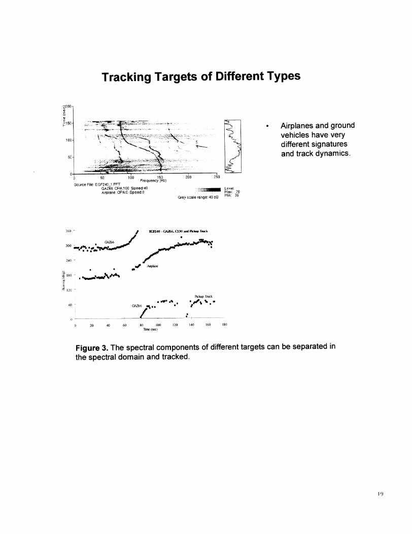
Tracking Targets of Different Types

-

180

0 20 40 60 80 100 120 140 160 180

Tine (sec)

Figure 3. The spectral components of different targets can be separated inthe spectral domain and tracked.

19

200-1)

1012-

512

5J iào 10Frequency (Hzj

Source File EGF24O_1 .FFTGAZ6B CPA:100 Speed:40Airplane OPA:O Speed:0

• Airplanes and groundvehicles have verydifferent signaturesand track dynamics.

20 250

LevelMax: 70

GreysaIerariqe:4008Me. 36

360 - R24O-G6,Q3OaII1P4aTUk

300

240 T

120

60

I •

GAZ66/Pekup Truck

.•y•.%.. 'P

20

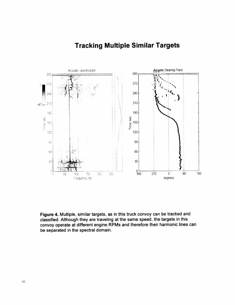
Tracking Multiple Similar Targets

Acousc petroaram

Figure 4. Multiple, similar targets, as in this truck convoy can be tracked andclassified. Although they are traveling at the same speed, the targets in thisconvoy operate at different engine RPMs and therefore their harmonic lines canbe separated in the spectral domain.

U(I)

EH

0degrees

Linear Map with single meancannot distinguish betweenshaded and unshaded regions

Non Linear Map with multiple meanscan distinguish betweenshaded and unshaded regions

Figure 5. The feature vectors of some targets show substantial variationsdepending on vehicle speed and operating gear. Their feature vectors canbe spread out over disjoint regions of the feature space, requiring a non-linear mapping function to describe them.

An ACON structure An OCON structure

Figure 6. ACON (All Class in One Network) and OCON (One Class inOne Network) Architectures. In each case the input vector is the same.In the ACON one network computes the output vector for all classes. InOCON multiple networks are used to compute the output vector.

21

Feature A