influence of mixture composition on washout resistance, fresh ...
Upload
khangminh22Category
view
2download
0
Grace Njenga
March, 2016
SUPERVISORS:
Ms. Dr. Ir. W. Bijker
Dr. V.A. Tolpekin
Multiple Endmember Spectral Mixture Analysis (MESMA) on multi-temporal VHR images for weed detection in smallholder farms.


Thesis submitted to the Faculty of Geo-Information Science and Earth
Observation of the University of Twente in partial fulfilment of the
requirements for the degree of Master of Science in Geo-information
Science and Earth Observation.
Specialization: Geoinformatics
SUPERVISORS:
Ms. Dr. Ir. W. Bijker
Dr. V.A. Tolpekin
THESIS ASSESSMENT BOARD:
Chairman: Prof. Dr. Ir. A. Stein, ITC
Ms Dr. I.C. van Duren, (External Examiner, University of Twente,
ITC-NRS)
Multiple Endmember Spectral Mixture Analysis (MESMA) on multi-temporal VHR images for weed detection in smallholder farms.
GRACE NJENGA
Enschede, The Netherlands, March, 2016

DISCLAIMER
This document describes work undertaken as part of a programme of study at the Faculty of Geo-Information Science and
Earth Observation of the University of Twente. All views and opinions expressed therein remain the sole responsibility of the
author and do not necessarily represent those of the Faculty.

i
ABSTRACT
Acquiring accurate weed information remains a challenge in agricultural crops due to the weed’s high
spectral variability and the number of weed species within a crop field. The weed fraction is detected based
on variations in the spectral response of the plant canopy and depends on the species and the weed density
present. In this thesis, the potential of multispectral satellite remote sensing and Multiple Endmember
Spectral Mixture Analysis (MESMA) is evaluated for the detection of weed infestation in maize (Zea mays
L.), Cotton (Gossypium hirsutum) and millet (Pennisetum glaucoma L.). Field boundaries, plots and quadrants
were laid out in three small-holder crop fields for the experiment by the STARS project in Soughumba, Mali
and each field had an area of less than two hectare’s. Multi–spectral images consisting of 8 bands obtained
by the WorldView-2 satellite platform were used. Spectral libraries were extracted using the Sequential
Maximum Angle Convex Cone (SMACC) algorithm, followed by the Spectral Matching Algorithm (SMA)
for the identification of unknown spectra. Spectral information of crops and weeds, as well as the soil
contribution, need to be analysed. Utilization of this information across multiple dates of imagery requires
approaches for building spectral libraries and for classification. MESMA, which is an improvement of
Simple Linear Spectral Mixture Analysis (SLSMA) was employed in this study to accommodate spectral and
temporal variability associated with weeds and crops commonly observed in agricultural fields. However,
endmember selection is a critical step in the application of MESMA. For comparison, simple Linear Spectral
Mixture Analysis (SLSMA) was also used. SLSMA does not account for spectral variations present within
the same material, since it permits only one endmember per crop/weed class. MESMA addresses these
concerns by allowing endmembers to vary on a per-pixel basis. Two MESMA endmember selection
techniques were applied: Endmember Average Root Mean Square Error (EAR) and Minimum Average
Spectral Angle (MASA). A four endmember-model (crop, weed, soil and shadow) was used to un-mix each
image independently. The results were compared to the number of endmembers selected, the percentage of
image pixels modelled, the weed fraction estimate and correlations with the ground reference data to
determine the most accurate method for weed-crop discrimination. The MASA endmember selection
technique outperformed the EAR by having a higher percentage of image pixels modelled and also higher
correlations with the ground reference data across all the dates and in all crop fields. This research has shown
that weed densities vary from field to field as well as within–field. Statistical analysis of the modelled weed
fraction was carried out to determine the accuracy of the fraction estimates. The MESMA results were more
accurate when compared to SLSMA. Finally, the modelled weed fractions were validated using root mean
square error (RMSE), standard error (SE) and the coefficient of determination (R2). The relationship
between the estimated and observed weed densities was satisfactory, the highest coefficient of determination
for the cotton field was R2=0.722, RMSE=0.041 and an SE= 0.003 on September 29th while the lowest was
on October 18th with an R2=0.591, RMSE=0.043 and SE= 0.001 for the MASA results. The highest
coefficient of determination for the EAR weed fraction was R2=0.717, RMSE=0.051 and an SE= 0.006 on
September 29th and the lowest EAR fraction was observed on October 18th an R2=0.566, RMSE=0.049 and
SE= 0.006. For the SLSMA weed fraction results, the highest coefficient of determination for the cotton
field was R2=0.584, RMSE=0.058 and an SE= 0.028 on September 29th while the lowest was recorded on
October 18th with an R2=0.501, RMSE=0.059 and SE= 0.024 were recorded. Multi-temporal imagery has
the potential for discriminating early and late-season weed infestations across a range of crop growth stages.
Furthermore, this research demonstrated the ability of MESMA to accurately model the total vegetation
cover fraction in pixels. Evaluation of vegetation indices for the detection of vegetation (weeds and crops
together) showed that the World-View Improved Vegetative Index (WV-VI), which uses NIR2, showed the
highest correlation with the Fcover across all the fields.

ii
ACKNOWLEDGEMENTS
First, I would like to thank God for his goodness, wisdom, knowledge, health and breakthroughs I
experienced throughout my study. I would like to express my sincere gratitude to my supervisors Dr. Ir.
Wietske Bijker and Dr. Valentyn Tolpekin for their continuous support of my research, for their patience,
motivation enthusiasm, and immense knowledge. Thank you for the inspiration and valuable wisdom I
obtained working with you in the thesis period. Your support, guidance and encouragement were invaluable.
I very much appreciate the confidence they showed in me for undertaking this research topic. Also to the
GFM department, thank you so much knowledge I obtained throughout my study, it has surely equipped
me for the future.
I would also like to thank the STARS project and ICRISAT for providing me with the data for this project.
My sincere thanks to the Netherlands Government through the Netherlands Fellowship Programme (NFP)
for funding my MSc at the Faculty of Geo-Information Science and Earth Observation, University of
Twente (ITC). I wish to devote this thesis to my family, colleagues at work and friends whose love, sacrifice,
and devotion towards me cannot be described adequately by words, for their unconditional support and
reminding me about the real important things in life.
To all my GFM classmates, you made the journey worthwhile. Thank you all for the encouragement and
fun throughout the duration of the course.

iii
TABLE OF CONTENTS
Abstract ............................................................................................................................................................................ i
Acknowledgements ....................................................................................................................................................... ii
List of figures ................................................................................................................................................................ vi
List of tables ............................................................................................................................................................... viii
List of Photos ............................................................................................................................................................. vix
List of abbreviations ...................................................................................................................................................... x
1.0 INTRODUCTION .............................................................................................................................................. 1
1.1. Background of the study ............................................................................................................................................1 1.2. Motivation.....................................................................................................................................................................1 1.3. Problem statement ......................................................................................................................................................2 1.4. Research identification ...............................................................................................................................................3
1.4.1. Specific research objectives ..................................................................................................................... 4
1.5. Research questions ......................................................................................................................................................4 1.6. Innovation ....................................................................................................................................................................4 1.7. Thesis structure ............................................................................................................................................................4
2.0 LITERATURE REVIEW ................................................................................................................................... 7
2.1. Agriculture in Sub-Saharan Africa ............................................................................................................................7 2.2. Weed detection ............................................................................................................................................................7
2.2.1. Site-specific weed management .............................................................................................................. 7
2.2.2. Use of remote sensing data ..................................................................................................................... 8
2.2.3. WorldView-2 imagery ............................................................................................................................... 8
2.3. The effects of weed on the yield ...............................................................................................................................8 2.4. Subpixel Classification ................................................................................................................................................9
2.4.1. Spectral mixture analysis (SMA) ............................................................................................................. 9
2.5. Spectral mixture analysis methods ......................................................................................................................... 11 2.6. Simple linear spectral mixture analysis .................................................................................................................. 11
2.6.1. Endmember extraction ......................................................................................................................... 11
2.6.2. Multiple endmember spectral mixture analysis (MESMA) ............................................................. 12
2.6.3. Application of MESMA ........................................................................................................................ 17
2.6.4. Limitation of Spectral Mixture Analysis ............................................................................................. 17
2.7. Temporal analysis using vegetation indices (VIs) ............................................................................................... 17
2.7.1. Types of vegetation indices .................................................................................................................. 18
2.8. Class separability analysis ........................................................................................................................................ 18 2.9. Accuracy assessment ................................................................................................................................................ 19
3.0 STUDY AREA AND DATA DESCRIPTION .......................................................................................... 21
3.1. Study Area .................................................................................................................................................................. 21 3.2. Data description ........................................................................................................................................................ 22
3.2.1. Earth observation data .......................................................................................................................... 22
3.2.2. Ground reference dataset ..................................................................................................................... 23
3.2.3. Crop development stages/crop Calendar .......................................................................................... 23
3.2.4. Fertility treatments ................................................................................................................................. 24
3.2.5. Seasonal canopy development ............................................................................................................. 25
3.2.6. Procedure for ground cover measurement ........................................................................................ 25
3.3. Field photographs..................................................................................................................................................... 26 3.4. Weed species identified in millet/maize fields in the study area. ..................................................................... 26

iv
3.4.1. Striga Spp. .................................................................................................................................................. 26
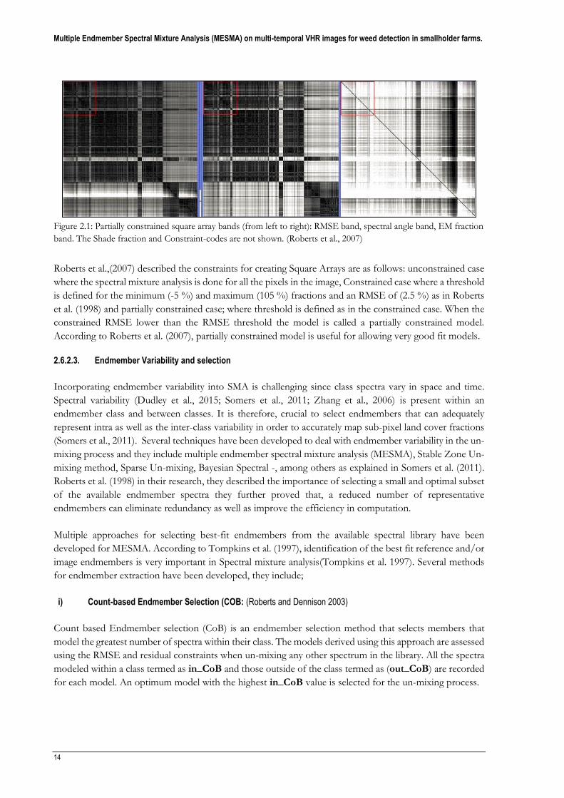
3.4.2. Digitaria horizontalis (crab-grass) ............................................................................................................ 27
3.4.3. Cynodon dactylon ........................................................................................................................................ 27
3.4.4. Cyperus rotundus ......................................................................................................................................... 27
3.4.5. Echinochloa colona ...................................................................................................................................... 28
3.4.6. Rottboellia cochinchinensis ........................................................................................................................... 28
3.4.7. Commelina forskalaei .................................................................................................................................. 29
3.4.8. Cenchrus biflorus ......................................................................................................................................... 29
3.4.9. Amaranthus viridis, .................................................................................................................................... 29
3.4.10. Imperata cylindrica ...................................................................................................................................... 30
3.4.11. Sonchus oleraceus (sow-thistle) .................................................................................................................. 30
4.0 METHODOLOGY .......................................................................................................................................... 31
4.1. Introduction to methodology ................................................................................................................................. 31 4.2. Data preparation and preprocessing ..................................................................................................................... 31
4.2.1. Image preprocessing ............................................................................................................................... 32
4.3. Vegetation indices analysis ...................................................................................................................................... 33 4.4. Spectral mixture analysis ......................................................................................................................................... 34
4.4.1. Multiple endmember spectral mixture analysis (MESMA) .............................................................. 34
4.4.2. Simple Linear Spectral Mixture Analysis............................................................................................. 37
4.5. Endmember separability ......................................................................................................................................... 38
4.5.1. Transformed divergence (TD) .............................................................................................................. 38
4.5.2. Jeffries Matusita (JM). ............................................................................................................................ 38
4.6. Accuracy assessment ................................................................................................................................................ 40
5.0 RESULTS AND DISCUSSION ..................................................................................................................... 41
5.1. Results ........................................................................................................................................................................ 41
5.1.1. What is the relationship between the Fcover and vegetation indices? ........................................... 41
5.1.2. Which VI is best suited for the crop field vegetation mapping using correlation analyses ........ 43
5.1.3. Vegetation index images ........................................................................................................................ 45
5.2. Spectral mixture analysis ......................................................................................................................................... 47
5.2.1. Results of Simple Linear Spectral Mixture Analysis (SLSMA) ........................................................ 47
5.3. Multiple Endmember Spectral Mixture Analysis (MESMA) ............................................................................ 49
5.3.1. Endmember extraction using SMACC ............................................................................................... 49
5.3.2. Creation of the metadata files for the unknown endmembers ........................................................ 52
5.3.3. Square array results ................................................................................................................................. 53
5.3.4. Selection of the optimal endmembers ................................................................................................. 55
5.3.5. What is the minimum class separability for the recognition of weed and the crop? ................... 55
5.4. MESMA unmixing and the classification results ................................................................................................ 59
5.4.1. What is the weed infestation percentage in the crop fields? ............................................................ 62
5.4.2. What is the comparison of the modelled weed with the reference weed fraction? ..................... 64
5.4.3. What is the comparison between the EAR and MASA results? ..................................................... 66
5.4.4. What is the comparison between the MESMA and SLSMA results .............................................. 70
5.4.5. What is the relationship between the modelled weed fraction and the WV-VI? ......................... 72
5.5. What are the pattern and spatial distribution of weeds in the crop fields? .................................................... 73
5.5.1. What is the qualitative comparison between the classification maps with the vegetation
indices? ..................................................................................................................................................... 75
5.5.2. What is the comparison between Fcover and MESMA results?..................................................... 77

v
5.5.3. What is the comparison between the Fcover and with Simple linear un-mixing vegetation
results ....................................................................................................................................................... 78
5.6. Discussion .................................................................................................................................................................. 79
5.6.1. Spectral variability and separability between Crops and weeds ...................................................... 81
5.6.2. Vegetation indices .................................................................................................................................. 82
5.7. Limitation of the study ............................................................................................................................................ 83
6.0 CONCLUSION AND RECOMMENDATIONS ..................................................................................... 85
6.1. Conclusion ................................................................................................................................................................. 85 6.2. Recommendations .................................................................................................................................................... 87
References……………………………………………………………………………………………………….89

vi
LIST OF FIGURES
Figure 2.1: A Graphical representation of a linear mixture model. .................................................................... 10
Figure 2.2: Partially constrained square array bands (from left to right): RMSE band, spectral angle band,
EM fraction band. The Shade fraction and Constraint-codes are not shown. ................................................ 14
Figure 2.3: A is the endmember and B is the modelled spectrum A. ρ1 and ρ2, are vectors with reflectance
components bands, f is the endmember A fraction. RMSE and spectral angle error metrics are indicated
by the solid and dashed lines, respectively.. ............................................................................................................ 16
Figure 3.1: A Map showing the study area. The left image shows the agro-pastoral map of Mali, (middle,
the September 29th satellite image and right shows the study fields. ................................................................. 22
Figure 3.2: A Conceptual sampling design. Source: STARS-Project-Data collection protocol...................... 24
Figure 3.3: The position of the quadrats within the plot. The green and blue tags were used to retrieve
information for the measured plant with red tag get lost during the season. Source: STARS-Project-Data
collection protocol. ..................................................................................................................................................... 25
Figure 3.4: Ground cover estimation: a): vertical picture acquisition (b): picture processing with CAN-
EYE freeware and c) resulting plant/soil classification. ....................................................................................... 25
Figure 4.1: Plots and quadrats distribution in the crop field. The letter A-F refers to the plots while the
number refers to the quadrat. The dots refer to the spatial location of the quadrat ........................................ 31
Figure 4.2: The analysis procedure of VIs mapping with high-resolution WV-2 imagery .............................. 34
Figure 4.3: The endmember estimation and extraction process .......................................................................... 35
Figure 4.4: The flowchart showing the spectral mixture analysis ........................................................................ 39
Figure 1.1: Mean of vegetation indices MSAVI2, MTVI2, NDVI, SARVI, TNDVI and WV-VI temporal profiles per image date and their standard deviations for the cotton (27), millet (26) and maize (2) fields………………………………………………………………………………………………….…42 Figure 1.2: Scatter plots showing the relationship between the Fcover and vegetation indices (NDVI, MSAVI2 and WV-VI) for the cotton field in September 29th……………………………..…………….44 Figure 1.3: WV-VI profiles for the cotton, maize and millet crop fields…………………………………44 Figure 1.4: The WV-VI for the July 29th, October 18th, November 1st and November 14th for the cotton field …..……………………………………………………………………………………………....…45 Figure 1.5: WV-VI for the July 29th, October 18th and November 14th for the maize field …..…...........…46 Figure 1.6: The WV-VI for the July 29th, October 18th and November 14th for the millet field……..……46 Figure 3: Relation between the crop and weed fractions modelled using SLSMA………………………..48 Figure 1.8: SMACC output: from left: A graph showing the behaviour of the maximum relative error (MRE) based on the number of endmembers in SMACC; (right) - Abundance map for Endmember 3 (September image) representing the cotton crop overlaid with the field boundary; spectral library plots (bottom)……………………………………………………………………………………………..….49 Figure 1.9: Spectral library plots for the cotton, millet and maize fields. (From left to right): September 29th, October 10th and October 18th extracted using SMACC…………………………………………51 Figure 1.10: The reference spectral libraries for the cotton millet and maize fields showing the spectra representing different weed infestation levels…………………………………………………...……….52 Figure 1.11: The partially constrained square array bands (from left to right): Shade fraction, RMSE band, EM fraction band, spectral angle band, and the Constraint-codes for all the image dates. (Table 5.5 below shows the mean values for the cotton field for the square array…………………………………………54 Figure 1.12: Graphical representation of TD separability indices between the 3 endmember selection methods per date for the millet and maize …………………………………………………………...…56 Figure 1.13: Graphical representation of TD separability indices between the 3 endmember selection methods per date for the cotton field……………………………………………………………...…….57 Figure 1.14: Graphical representation of JM separability indices between the 3 endmember selection methods per date for the millet, maize and cotton field……………………………. …………………..58 Figure 1.15: Weed fraction images per date for the cotton field modelled using EAR endmembers…..…59 Figure 1.16: Weed fraction images per date for the cotton field modelled using MASA endmembers …..60

vii
Figure 1.17: Weed fraction images per date for the millet field modelled using MASA endmembers….....60 Figure 1.18: Weed Fraction images per date for the maize field modelled using EAR endmembers (top image) and MASA endmembers (bottom image)……………………………………………………….. 61 Figure 1.19: Scatterplots showing the relationship between the EAR-modelled weed fraction and the reference weed fraction for the cotton fields. ………………………………………………………..….66 Figure 1.20: Relationship between EAR and MASA un-mixing weed fraction for the cotton (27), maize (2) and millet (26) with reference to time………………………….…………………………………… …..67 Figure 1.21: Scatterplots showing the relationship between EAR and MASA un-mixing weed fraction for the cotton (27), maize (2) and millet (26) for the September 29th image……………………………....….69 Figure 1.22: Temporal profiles showing the relationship between the MESMA (EAR and MASA) and SLSMA weed fractions for the cotton field (27), the millet field (26) and maize field (2)………….……..71 Figure 1.23: Comparison between EAR, MASA and simple SMA modelled weed fractions with a reference from the Ground reference data for the in plot A, recorded on September 29th for the cotton field….…72 Figure 1.24: The EAR classification (top) and MASA classification (bottom) image per date for the cotton field……………………………………………………………………………………………………..73 Figure 1.25: The EAR classifications (top) and MASA classification (bottom) image per date for the maize field……………………………………………………………………………………………………..73 Figure 1.26: The MASA Classification images per date for the millet field………………………...…….74 Figure 1.27: The comparison between the MESMA (weed and crop) classification image with WV-VI for the cotton field with reference to date using the MASA modelled fractions……………….…………….74 Figure 1.28: The comparison between the SLSMA (weed and crop) classification image (top) with WV-VI (bottom) for the cotton field with reference to date……………….…………………………………….75 Figure 1.29: The comparison between MESMA (EAR and MASA) modelled vegetation (weed + crop) and the Fcover for the cotton, millet and the maize fields…………………….……………………………...77 Figure 1.30: The comparison of the R-squared coefficients of the (modelled vegetation in relation to the Fcover) between MESMA (EAR and MASA) and SLSMA with reference to time………………………79

viii
LIST OF TABLES
Table 3.1: WV-2 multispectral sensor bands: ......................................................................................................... 23
Table 3.2: BBCH decimal Code for growth stage of the crops ........................................................................... 24
Table 3.3: Weed Species Identified in the millet fields quadrats in Mali ............................................................ 26
Table 4.1: The formulae for computation of the vegetation indices .................................................................. 33
Table 5.1: Mean of vegetation indices MSAVI2, MTVI2, NDVI, SARVI, TNDVI and WV-VI per image
date and their standard deviations for the cotton (27), millet (26) and maize (2) fields. ................................. 41
Table 5.2: The Relationship between Fcover and VIs in the three fields. The relationships exhibit
significant correlations. ............................................................................................................................................... 43
Table 5.3: Shade Normalized simple linear un-mixing weed, crop and soil fractions...................................... 47
Table 5.4: Metadata file for spectral library for the cotton field on September 29th ........................................ 53
Table 5.5: Mean values for cotton field square array per image date .................................................................. 54
Table 5.6: The endmember selection by date for the cotton field. ..................................................................... 55
Table 5.7: TD separability indices for the three fields using representative endmembers selected by various
techniques. See Figure 5.11 for graphical representation...................................................................................... 56
Table 5.8: The JM separability indices for the three fields using representative endmembers selected by
various techniques. See Figure 5:13 for graphical representation........................................................................ 57
Table 5.12: Comparison between the EAR and MASA modelled image/pixel percentage ........................... 70
Table 5.13: The correlations results between the WV-VI and the derived weed fractions for the Cotton,
maize and millet fields. ............................................................................................................................................... 72
Table 5.14: Evaluation of the modelled vegetation fraction in comparison to Fcover ................................... 78
Table 5.15: Comparison between the Fcover and with modelled vegetation using SLSMA .......................... 78

ix
LIST OF PHOTOGRAPHS
Photo 1: Photograph showing weed infestation in Millet Field. ........................................................................... 3
Photo 2: Striga hermonthica. & Photo 3: Striga asiatica .......................................................................................... 27
Photo 4: Digitaria horizontalis. ................................................................................................................................... 27
Photo 5: Cynodon dactylon. .......................................................................................................................................... 27
Photo 6: Cyperus rotundus. .......................................................................................................................................... 28
Photo 7: Echinochloa colona. ........................................................................................................................................ 28
Photo 8: Rottboellia cochinchinensis. ............................................................................................................................. 28
Photo 9: Commelina forskalaei. ................................................................................................................................... 29
Photo 10: Cenchrus biflorus. ......................................................................................................................................... 29
Photo 11: Amaranthus viridis. ..................................................................................................................................... 29
Photo 12: Imperata cylindrica. ..................................................................................................................................... 30
Photo 13: Sonchus oleraceus. ........................................................................................................................................ 30
Photo 14: Cotton field between July and November 2014 showing changes in temporal changes in
vegetation cover .......................................................................................................................................................... 47
Photo 15: Cotton field between August and November 2014 showing different weed proportions. ........ 63
Photo 16: Millet field between June and November 2014 showing different weed proportions. ............... 63
Photo 17: Maize field between August and November 2014 showing different weed proportions ............. 64
Photo 18: Millet field weed fraction estimation using field photographs .......................................................... 64
Photo 19: Photograph showing spectral heterogeneity within a maize field .................................................... 80
Photo 20: Photographs showing causes of reduced weed fractions. Top: weeding, middle row, canopy
closure, bottom: irrigation/flooding - killing weeds between crop rows .......................................................... 81

x
LIST OF ABBREVIATIONS
6S - Simulation of a Satellite Signal in the Solar Spectrum
AGB - Above‐Ground Biomass
ARVI - Atmospheric Resistant Vegetation Index
BD - Bhattacharyya Distance
BRDF - Bidirectional Reflectance Distribution Function
CoB - Count-Based Endmember Selection
CRES - Constrained Reference Endmember Selection
DEM - Digital Elevation Model
EAR – Endmember Average RMSE
EM - Endmember
ENVI - Environment for Visualizing Images
GFRAS - Global Forum for Rural Advisory Service
GNSS - Global Navigation Satellite System
GPS - Global Position System
ICRISAT - International Crops Research Institute for the Semi-Arid Tropics
IDL - Interactive Data Language
JM - Jeffrey’s Matusita
LAI - Leave Area Index
LSMA -Linear Spectral Mixture Analysis
MASA - Minimum Average Angle
MESMA - Multiple Endmember Spectral Mixture Analysis.
MODIS - Resolution Imaging Spectro-Radiometer
MSAVI - Modified Soil adjusted vegetation index
MTVI2 - Modified Triangular Vegetation Index
NIR - Near infrared region of the spectrum.
NDVI - Normalized Difference Vegetation Index
PPI - Pixel purity index
RMSE –Root Mean Square Error.
R2- R squared
RDVI - Renormalized Difference Vegetation Index
ROI - Region of Interest
SAM -Spectral angle mapper.
SARVI- Soil and Atmospherically Resistant Vegetation Index
SAVI -Soil adjusted vegetation index
SMA - Spectral mixture analysis
SMACC - Sequential Maximum Angle Convex Cone
STARS - Spurring a Transformation for Agriculture through Remote Sensing
SE – Standard Error
SSWM – Site-Specific Weed Management
TNDVI - Transformed Normalized Difference Vegetation Index
TD -Transformed Divergence
WV- WorldView
WV-VI -World-View Improved Vegetative Index

Multiple Endmember Spectral Mixture Analysis (MESMA) on multi-temporal VHR images for weed detection in smallholder farms.
1
1.0 INTRODUCTION
1.1. Background of the study
The agricultural sector is increasingly becoming a knowledge-based industry in response to economic and
environmental factors (Herwitz et al. 2004). To help meet the need for observational data, aircraft and
satellite remote sensing technology are playing an important role in farm monitoring and management as in
LeBoeuf (2000) & Lu et al., (1997). In their research Iizumi and Ramankutty (2015), the agricultural yields
primarily depend on weather conditions and farm management practices. One of the major key constraints
that hinders increased crop production is a lack of weed control. The key operation that needs improvement
is the timely removal of weeds. Weed monitoring is important for better management of agricultural food
production which is a key sector in developing countries and most especially in Sub-Saharan African
countries like Mali; whose agricultural production is adversely affected by poor farm management practices
(Diarra and Kangah 2007). Categorized as one of the least developed countries, Mali’s population heavily
relies on small-holder subsistence farming. In Diarra and Kangah (2007), less than 4 % of Mali land is used
for agriculture. Therefore proper farm management practices such as weed management are crucial for
maximum production from agricultural fields (Passioura 2006).
Detection of weeds has been used for site-specific weed management (SSWM) (Heege 2013). Quantifying
and mapping weeds in crop fields provide crucial information to farmers and various agricultural decision
support (Herwitz et al. 2004) and monitoring institutions at different stages of the crops growth. This is
possible through either rigorous field surveys or use of advanced remote sensing imagery and techniques.
Ground-based field surveys are expensive and time-consuming (Singh et al., 2011) but have continued to be
used in Africa causing delays in data collection and eventually delayed advice to the farmers and other
agricultural stakeholders. Ramesh et al. (2010) described this delay as greatly affecting continuous
assessments in the field of agriculture.
1.2. Motivation
Weed detection has been widely done for site-specific weed management and is mainly done for large
mechanized farms (Brown & Noble, 2005; Jurado-Expósito et al., 2003; López-Granados, 2011; Shaw, 2005;
Torres-Sánchez et al., 2013). The relevance of this research is intended for weed mapping using WV-2
multispectral images in small-holder farming systems with farm size being less than two hectares (STARS-
Project 2015). Despite the small size of the fields where farmers can easily detect weeds manually, however
not all the fields are weeded on time leading to yield loss. Some very noxious weeds like Striga species
occurring in maize and millet fields are prone to the research fields and have been reported to cause massive
damage to crops (Bengaly et al., 1998; Cabi, 2015; Clark et al., 1994). According to Goel et al. (2003) & Peña
et al. (2013), there is a need for information to farmers and agricultural decision makers regarding the effects
of early/late weeds infestations on the crop yield. Weeds and crops compete for moisture, light, nutrients
and can cause high toxicity effect leading to interference in crop growth (Ansong and Pickering 2015).
Weed mapping can effectively be done using remote sensing (Lopez-Granados et at., 2006; Smith &
Blackshaw, 2003; Toothill, 2009), however, the results of weed mapping are greatly affected by the spatial-
temporal resolution of the input image. This has led to high-resolution information needs that are driving

Multiple Endmember Spectral Mixture Analysis (MESMA) on multi-temporal VHR images for weed detection in smallholder farms.
2
further the technological innovations according to Schaepman et al. (2009) in small-holder farming and
other agricultural applications according to Herwitz et al. (2004).
Detection and quantification of weeds in crop fields using satellite imagery have not been easy in Mali, mainly due to lack of technical know-how on how to use the technology and its high cost (Byrd et al., 2014; Lass & Callihan, 1997; Rembold et al., 2013). Weed mapping is made possible in this research through the support of the STARS (“Spurring a Transformation for Agriculture through Remote Sensing”) project which is actively involved in facilitating the use of very high-resolution remote sensing data and field data collection. This provision as well as processing and analysis of data is to improve livelihoods of small-holder farmers with a less than two hectare crop field land who also face adverse weather conditions (STARS-Project 2015) and poor farm management techniques leading to low crop production. This research analyses the weed occurrence proportions in millet, cotton and maize fields and the individual or combined spectral signatures on very high resolution remotely sensed images at detailed scale using spectral mixture analysis. This facilitates understanding of the relation between weeds and crops and quantifying them as accurately as possible.
This research analyses the weed occurrence proportions in millet, cotton and maize fields and the individual
or combined spectral signatures on very high resolution remotely sensed images at detailed scale using
spectral mixture analysis, Multiple endmember spectral mixture analysis (MESMA) which uses more than
one endmembers per class to correct for within-class variability is used in this research for weed detection
and for comparison purpose, simple linear spectral mixture analysis (SLSMA) is also applied. For the
accurate application of Simple linear spectral mixture analysis, endmember selection is very important. The
key to MESMA is to detect which spectra in a group of spectra are the best representative of a class they
represent while covering the range of variability within the class. Endmember Average Root mean square
error (EAR) (Dennison & Roberts, 2003a) which selects endmembers with the lowest RMSE and the
Minimum Average Spectral Angle (Dennison et al., (2004) which selects endmembers with the lowest
spectral angle between two spectra are used for the endmember selection.
1.3. Problem statement
Crops and weeds mapping involves a careful understanding of their local and site-specific heterogeneity
(Rossi, Giosuè, & Caffi, 2010; Torres-Sánchez et al., 2013), type of weed and association with the crop. Due
to wide and complex weeds species variability (Lee et al., 2010; Piron et al., 2010), weeds identification is a
challenge. Very limited techniques are available to detect weeds against crop plants in the field. The use of
the spectral characteristics to discriminate between the crops and weeds (Alchanatis et al., 2005; Martín et
al., 2011; Pérez, 2000; Vioix et al., 2002) relies mostly on the weed infestation levels in the scene. Images
collected at low resolutions are not sufficient to detect small patches of weed (Shaw 2005). World-View
imagery shows a great potential for overcoming these limitations of other satellite remote sensing data due
to its superior spatial resolution.
Misclassification of crops and weeds, may arise when they have similar spectral characteristics (Peña-
Barragán et al., 2011) or in un-weeded fields or even when there is a variability in spectral reflectance
(Dennison et al., 2007; Dudley et al., 2015; Okin, et al., 2001; Zhang et al., 2006) of the same crop. Crops
and weeds are distinguished based on their spectral characteristics, spectral similarities between weeds and
crops lead to low-class separability (Foerster., 2012; Somers, 2011). Quantifying and mapping the weeds and
estimating their effects on the crop yield in these areas is more complicated due to spectral variability within
a field.

Multiple Endmember Spectral Mixture Analysis (MESMA) on multi-temporal VHR images for weed detection in smallholder farms.
3
Weeds and crops grow in mixture resulting into mixed pixels (Qiu et al., 2014). There exists a limited spectral
separability of crops and weeds during the early stages (Piron, van der Heijden, and Destain 2010) of crop
development with some weeds showing spectral similarity to the crop. Weeds and crops need to be
discriminated at the sub-pixel level (Ozdarici-Ok., 2015; Qiu et al., 2014). Compared to object-based
classification, Spectral un-mixing at the subpixel level identifies the proportion of each class in a pixel.
Subpixel classification is the most appropriate technique for crop/weed detection that leads to high
classification accuracies of spectral mixtures.
Photo 1: Photograph showing weed infestation in Millet Field. (STARS&ICRISAT 2014)
Weeds removal and crop canopy closure (blocking weeds from direct sunlight) reduces the amount of weeds
to fluctuate. Equally, a millet crop with weeds may look denser in remote sensing images than it really is,
this is especially when vegetation indices related to green biomass are used and therefore vegetation Indices
alone are not enough. Intra-class and inter-class spectral variability exist in the study field, to effectively map
this variability, a multiple endmember spectral mixture analysis (MESMA) is used for the weed fraction
estimation and classification. For comparison purposes, simple linear spectral un-mixing is also used to
evaluate the most accurate sub-pixel method for weed mapping. For accuracy assessment, the ground cover
fraction of the soil surface covered by green plant material (Fcover), Vegetation indices and the observed
weed fractions are used.
1.4. Research identification
The main objective of this research is to improve weed detection using the temporal (vegetation indices)
and spectral characteristics of weeds using vegetation indices(VI) and Multiple Endmember Spectral Mixture
Analysis (MESMA) on multi-temporal VHR images for weed detection in smallholder farms.
Based on the above-mentioned main objective, the following are the specific objectives and corresponding
research questions.

Multiple Endmember Spectral Mixture Analysis (MESMA) on multi-temporal VHR images for weed detection in smallholder farms.
4
1.4.1. Specific research objectives
1. To perform a comparative regression analysis to determine the relationship between the Fcover
and vegetation indices,
2. To determine which Vegetation Index is best suited for vegetation (crop+weed) mapping,
3. To detect weeds through spectral mixture analysis.
i) To identify the class separability for the recognition of weed and the crop,
ii) To determine the pattern and spatial distribution of the weeds in a crop field,
iii) To compute weed infestation percentage,
4. To perform a statistical analysis of the weed fraction modelled from WV-2 images and the field
data.
i) To determine the relationship between the modelled weed fraction and observed fraction
ii) To determine the relationship between the modelled weed fraction and VIs
iii) To compare EAR and MASA endmember selection techniques
iv) To evaluate the classification accuracy between MESMA and simple linear spectral
mixture analysis
v) To determine the relationship between the modelled vegetation with the Fcover
1.5. Research questions
1. What is the relationship between the Fcover and vegetation indices?
2. Which VIs are the most suitable for vegetation (crop/weed) mapping?
3. What is the pattern and spatial distribution of weeds?
4. What is the maximum class separability for the recognition of weed?
5. What is the weed infestation percentage in the crop field?
6. What relationship between the SMA-modelled weed fraction and reference weed fraction?
7. What is the relationship between the between the modelled weed fraction and VIs?
8. What is the comparison between EAR and MASA endmember selection techniques?
9. What is the classification accuracy between MESMA and simple linear spectral?
10. What is the relationship between the modelled vegetation with the Fcover?
1.6. Innovation
Weeds and crops occur in a mixture. Previous studies done on weed detection have basically relied on
the object based classification taking the advantage of the weeds between the rows and disregarding
the intra-row weeds which have the possibility of underestimating the amount of weeds in a crop a
field. Through the use of spectral mixture analysis, both inter-row and intra-row weeds can be
determined, and this improves the accuracy of detection. The use of spectral mixture analysis to
identify the proportion of weeds in a crop field and more specifically the use of multiple endmembers
spectral mixture analysis which accounts for the spectral variability within improves the detection
accuracy in millet field. The method is also extended to cotton and maize fields.
1.7. Thesis structure
This thesis is organized into six chapters. Chapter one describes the motivation, problem statement
and research identification describing the main as well as the specific objectives accompanied by the
research questions addressed in this research. Innovation aimed at is also explained in this chapter.
Chapter 2 is the review of the previous studies regarding this research where the past and recent
literature are reviewed to identify the gaps to be filled by this research. Chapter 3 describes the study
area, data and materials used. The justification of the selected method used in this research and the
framework of the methodology are described in chapter 4. An implementation of the vegetation indices

Multiple Endmember Spectral Mixture Analysis (MESMA) on multi-temporal VHR images for weed detection in smallholder farms.
5
and the spectral unmixing technique on Worldview-Multispectral images is done in Chapter 5 in which
results and discussion are explained based on the specific objectives. The conclusion of this research
based on the research question as well as the recommendations for further research is presented in
chapter 6.

Multiple Endmember Spectral Mixture Analysis (MESMA) on multi-temporal VHR images for weed detection in smallholder farms.
6

Multiple Endmember Spectral Mixture Analysis (MESMA) on multi-temporal VHR images for weed detection in smallholder farms.
7
2.0 LITERATURE REVIEW
In this chapter, previous work and literature are reviewed. This chapter is subdivided into the following
subheadings; agriculture in sub-Saharan Africa, use of remote sensing, weed detection techniques, vegetation
indices and accuracy assessment. This chapter is used to justify the methodology developing process. It
provides an overview of the most important information and methods regarding this research.
2.1. Agriculture in Sub-Saharan Africa
Weeds-Crop identification and quantification of agricultural crops has not been easy in sub-Saharan Africa.
In Biradar and Xiao (2011), agricultural census statistics shows much information on the distribution of
crop types and total cropland area but spatial characteristics per field and weed distribution in this regard is
limited. In Mali, the locally available information on weeds distribution, crop type, acreage and cropping
season is unreliable. This unreliability is due to inadequate field data collection methods, lack technical
know-how in the application of the methods, the cost and time involved in data collection are high, leading
to only in a few locations are sampled which mostly are not representative. In order to maximize crop
production in small-holder farms in Sub-Saharan Africa, the farmers use different cropping patterns (both
row and broadcasting) based on agro-climatic, socio-economic, political and historical factors as described
in Bharathkumar and Mohammed-Aslam (2015). Most crop fields are not weeded on time, resulting in a
competition for nutrients and water between the weeds and the crops, further reducing the quantity and
quality of the yield. Information on weed management and the expected returns from these fields is crucial
to the farmers as well as agricultural decision makers to facilitate informed decision making.
2.2. Weed detection
2.2.1. Site-specific weed management
Weed species occur in non-uniform patches and as single stands across agricultural fields with the amount
of patchiness differing among weed species and crop fields. According to Lark et al. (1997), Selective
application of herbicides on the crop fields in large-scale farming requires an automated weed detection.
SSWM technology is mostly applicable in developed countries such as United States, Europe, China and
Australia where farming is mostly mechanized. López-Granados (2011) indicates a need for future
investigations to increase the acceptance and adoption of SSWM, however, the relevance of weed detection
in smallholder subsistence farms in Mali is not for SSWM. The farms parcels are less than 2 hectares
(STARS-Project 2015) and weeds could be easily detected and managed manually. The effect of weeds on
the crop production is of more importance to these small-holder farmers.

Multiple Endmember Spectral Mixture Analysis (MESMA) on multi-temporal VHR images for weed detection in smallholder farms.
8
2.2.2. Use of remote sensing data
Weed detection is probably the most successful application of airborne remote sensing in agriculture as
shown in the following research (Bryson et al., 2010; Gómez-Candón et al., 2013; Herwitz et al., 2004; Hung,
Xu, & Sukkarieh, 2014; Peña et al., 2013; Peña et al., 2015; Torres-Sánchez et al., 2015; Torres-Sánchez et
al., 2014; Torres-Sánchez et al., 2013). Satellite remote sensing has also been successfully used in identifying
and mapping several weed species (Backes & Jacobi, 2006; Dlamini, 2006; Karimi et al., 2006; López-
Granados et al., 2010; Martín et al., 2011; Pérez et al., 2000; Shapira et al., 2013; Shaw, 2005; Taylor et al.,
2010; Thorp & Tian, 2004). In order to accurately detect small patches of weeds in crop fields, there is a
great need to have high-resolution data sets in spatial-temporal and spectral resolutions. However, all these
virtues cannot be included into one satellite sensor for technical reasons thus selection of appropriate sensor
is important.
Sub-Saharan Africa is characterized by extreme climatic and weather conditions (Lee et al., 2010; Traore et
al., 2013), complex cropping systems (Zarco-Tejada et al., 2013) as well as varying spatial patterns in the
fields and diverse farming environments. Conventional methods of data collection are cumbersome,
expensive and time-consuming according to the STARS-Project (2015). The spatial complexity of the small-
holder farms coupled with mixed cropping systems and confounded with a high cost of obtaining high
spatial and high temporal resolution imagery according to Bendig et al. (2015) have prevented the use of
remote sensing technology in this region. There is therefore, a need for continual improvements in remote
sensing data acquisition technology to effectively and accurately map and quantify weed as well as
discrimination between weed species in the farms at reasonable costs.
2.2.3. WorldView-2 imagery
Recent remote sensing technologies such as Unmanned Aerial Vehicle (UAV) have proven to be
inexpensive, high in spatial resolution, and can be tasked to a high temporal resolution to obtain crop-
specific and/or weeds data (Herwitz et al., 2004; Hunt., et al., 2010; Peña et al., 2013; Peña et al., 2015;
Torres-Sánchez et al., 2015). Very High Resolution (VHR) satellite Imagery has been successively used in
mapping vegetation. For this study, weed/crop discrimination is done using Worldview-2 imagery with a
spatial resolution of 2 meters. Its high spatial resolution (Byrd et al., 2014; de la Fuente et al., 2013) can
provide crop-specific and/or weeds data. There are several vegetation mapping applications of the WV-2
imagery ranging from urban tree mapping to precision agriculture (Aguilar, et., al 2014; De la Fuente, et al.,
2013; Nouri, et al., 2014; Nunez-Casillas et al, 2012; Pu & Landry, 2012). The effects of the position and the
number of bands in WV-2 imagery has been studied previously leading to the conclusion that WV-2
additional bands (coastal blue, yellow, red-edge and NIR2) can improve the vegetation mapping accuracy
(Ngubane et al., 2014). A number of studies (Cho et al., 2012) noted the potential of WV-2 additional bands
in vegetation mapping. Using pixel-based approach, (Cho et al., 2012) identified that the WV-2 yellow band
is the most influential in vegetation mapping. WV-2 additional bands (yellow, red-edge and NIR2) have
been identified as most suitable for identifying vegetation species (Ngubane et al. 2014).
2.3. The effects of weed on the yield
The presence of weeds in crop fields leads to an increased green biomass making the field look denser in a
remote sensing image than it is really is. Weed control at an early growth stage of the crop is necessary for
the health of the plant. However, some weeds are difficult to map based on their reflectance due to spectral
similarity with the crop at an early stage of crop development, which is also characterized by a considerable
interference by the soil background reflectance as was studied by Thorp & Tian (2004).

Multiple Endmember Spectral Mixture Analysis (MESMA) on multi-temporal VHR images for weed detection in smallholder farms.
9
Various methods have been implemented in weed detection including; the use of spectral reflectance of
plants with neural networks (Cho, Lee, & Jeong, 2002); use of geostatistical method (Alchanatis et al. 2005);
use of object-based image analysis (Benz et al., 2004; Blaschke, 2010; Ling et al., 2012; Löw et al., 2015;
Peña et al., 2013; Peña-Barragán et al., 2011; Torres-Sánchez et al., 2015); wavelet method (Bossu et al.,
2009; Qiu et al., 2014), machine vision techniques (Meyer & Neto, 2008; Silva Junior,et al., 2012) and
Spectral mixture analysis (Jain et al., 2013; Ling et al., 2012; Small, 2012; Somers et al., 2011). As explained
earlier in this research, weeds and crops occur in mixtures and therefore for more accurate classification of
each component in a pixel, a sub-pixel classification is preferred.
2.4. Subpixel Classification
No matter the spatial resolution of an image, the spectral signatures collected in natural environments are a
mixture of different materials found within a single pixel. The pixel size of an image constrains the
resolution of the image as well as the detection capabilities of the objects in the image. Most land covers
occur in mixtures. A single pixel may consist more than one land cover type depending on its resolution.
For classification purpose, most researchers try to solve the problem of mixed signals using subpixel image
classification which derive the proportion of each cover type in a single pixel (Brown & Noble, 2005). Prior
knowledge of intra-species variation and inter-species variation is relevant to the accuracy of the final crop
and weeds identification (Zhang et al.,2006). Various methods subpixel classification method have been
developed. Commonly used are spectral mixture analysis and fuzzy classification. In (Foody & Cox 1994),
fuzzy classification requires a priori selection of the Fuzziness Exponent parameter which has remained to
be problematic. Moreover, the method is time-consuming and cumbersome and therefore not considered
for this research.
2.4.1. Spectral mixture analysis (SMA)
SMA classification method has been used to estimate land-cover fraction using remote sensing imagery
characterized by varied spatial, spectral and radiometric resolutions and temporal resolutions (Hussain et al.,
2013). A mixture model is a process of deriving mixed signals from pure endmembers while the spectral
un-mixing extracts the proportions of the pure endmembers from a mixed pixel. Several models have been
derived for determining the number of endmembers which include the most commonly used linear and the
nonlinear models (Dennison, Halligan, & Roberts, 2004; Jiang et al., 2006; Plaza & Plaza, 2011; Small &
Milesi, 2013). A linear mixture model has an assumption that the pixel variability in an image is caused by
the varying fractions of spectral endmembers. The linear spectral mixture model is based on the assumptions
that; the fractional abundance and a spectrum of each endmember are contained in a pixel (Plaza et al. 2011;
Somers et al. 2012). The other assumption is that most of the pixels in an image scene contain endmembers
that can be measured (Dennison & Roberts, 2003b). A linear mixing model is shown in Eq. 1 and Figure
2.1.

Multiple Endmember Spectral Mixture Analysis (MESMA) on multi-temporal VHR images for weed detection in smallholder farms.
10
Figure 2.1: A Graphical representation of a linear mixture model. (Martín 2013)
The Nonlinear spectral un-mixing model assumes that each pixel vector in an original image can be
modelled by the use of Eq. 2.
x = f (E, Φ) + n
Where f is the unknown non-linear function that defines the interaction between E and Φ.
According to Keshava (2003), non-linear mixtures are intimate mixtures of materials where the
radiation interacting with various substances before being directed back to the sensor leads to non-
linear spectral mixing radiation of multiple substances. Other models include the geometric and
stochastic-geometric models which take into the account the geometry and the distribution of the
object and the direction of solar radiation in order to evaluate the relative proportions of the object,
shadow and background in pixels. The stochastic geometric model is a special case of geometric models
that absorbs random radiation in its spatial structure. Probabilistic models are another type of models
Eq. 1
Eq. 2

Multiple Endmember Spectral Mixture Analysis (MESMA) on multi-temporal VHR images for weed detection in smallholder farms.
11
that are based on one of several probability techniques such as maximum likelihood as seen in Ichoku
and Karnieli (1996). Linear spectral mixture analysis has successfully been implemented in (Foody &
Cox, 1994; Liu et al., 2008; Plaza & Plaza, 2011; Tucker, 1979; Yang, Everitt, & Bradford, 2005).
2.5. Spectral mixture analysis methods
In many cases, a fixed number of endmembers is applied to an image in the implementation of spectral
mixture analysis, however, using a fixed number of endmembers does not account for within-class spectral
variability or/and spatial variability. Several methods have been devised to address the endmember
variability and similarity. Bateson et al. (2000) incorporated endmember variability into spectral mixture
analysis representing each endmember as a bundle of spectra. Roberts et al. (1998) introduced multiple
endmember spectral mixture analysis (MESMA) to allow the number and type of endmembers to vary per-
pixel. More studies that have involved endmember variability include; (Changshan et al., 2014; Dudley et al.,
2015; Li & Wu, 2015; Small & Milesi, 2013). According to Somers et al. (2011), MESMA has remained the
most widely used spectral mixture analysis technique for dealing with endmember variability.
2.6. Simple linear spectral mixture analysis
2.6.1. Endmember extraction
Potential representative endmember spectra can be collected from reference materials in a laboratory
(Roberts et al., 1993), they can be extracted from imagery (Bateson et al., 2000), or measured in the field
(Roberts & Herold, 2004). Endmembers that consist of distinct spectral characteristics are usually easy to
select. However, endmembers that have spectral similarities are more complex to discriminate Rogge et al.
(2007). Most commonly used endmember extraction techniques are based on the geometric analysis of an
image. These techniques include N-FINDR algorithm that determines simplexes from the largest volumes
within a dataset that contain the highest number of the pixels. N-FINDR does not require a priori
information about the endmembers but it is computationally time-consuming. The use of random initial
conditions also leads to inconsistencies of the results that are not reproducible.
Another algorithm is Pixel purity index (PPI)(Valdiviezo-N and Urcid (2012) which is based on the geometry
of the convex sets as in which generates many random n-dimensional vectors. This is a widely used method
but with a limitation that it is time-consuming and a cumbersome process that involves a visual inspection
and a lot of human intervention, especially in spectrally similar vegetation scenes. Other methods like
Support Vector Machine can be used to automatically extract endmembers. This method is fast and more
accurate compared to other methods.
Sequential maximum angle convex cone (SMACC) was developed by Gruninger et al. (2004) as an algorithm
for endmember extraction that uses a convex cone model to represent the vector data. The number of
endmembers to be extracted by SMACC are required to be known beforehand. For reflectance data an
RMSE tolerance of 1 % (Gruninger et al., 2004). An automatic shadow endmember is added when these
endmembers are used. Constraints such as the Sum to Unity constraint where the sum of the fractions
calculated for each pixel is equal to 100 %. When using the reflectance data either a positivity only (fractions
can only be positive) or sum-to-unity or less constraint is applied according to Gruninger et al., (2004).
Another parameter is Coalesce Redundant Endmembers which aggregates the SAM Coalesce value (a
parameter that aggregates redundant values into single spectra) within the specified spectral angle mapper
threshold into one endmember. Gruninger et al. (2004) specified that when distinguishing spectrally similar
materials, this parameter should not be used.

Multiple Endmember Spectral Mixture Analysis (MESMA) on multi-temporal VHR images for weed detection in smallholder farms.
12
SMACC finds the endmembers sequentially. A convex cone is formed by extreme vectors and model the
data that is within the cone. The dataset that lies outside the convex cone forms the residuals in the
constrained case. Oblique projections are used in the constrained case (Gruninger, Ratkowski, and Hoke
2004). The first endmember is defined by the convex cone determined by extreme points followed by a
constrained oblique projection to derive the second endmember while the convex cone is increased to
include the new derived endmember. This process goes on till the specified number of endmembers are
found (Gruninger, Ratkowski, and Hoke 2004). SMACC has proved to be an effective technique most
especially in extracting the endmembers of vegetation classes as demonstrated in Aggarwal and Garg (2015).
Endmembers extraction techniques have been extensively compared in the literature (Martínez et al., 2006;
Plaza & Martínez, 2004, Veganzones & Graña, 2008).
2.6.1.1. Spectral Matching
When dealing with known spectral and unknown spectral data i.e. known field collected spectra and
automatically collected unknown spectra. A quantitative comparison of surface reflectance of the known
spectra data set with unknown reflectance spectra is done using spectral matching techniques as in Kruse et
al., (1993). A measure of spectral similarity is done between the known and the unknown spectra. Another
method is the sub-pixel classification technique in Settle & Drake (1993) that derive the pixel fraction
estimates of a spectrally characterized materials as explained in Van der Meer (2006).
Spectral similarity measures were evaluated in Van der Meer (2006), these measures include the spectral
correlation measure in Van der Meer & Bakker (1997). This measure takes into account the relative shape
of the spectrum and the spectral match and therefore the resulting to statistic matches on the individual
absorption features (Van der Meer, 2006). The second method is the spectral angle measure described in
Kruse et al. (1993); other methods include is the Euclidean distance measure and the spectral information
divergence described in Chang (2000). Stein et al., (1998) used geostatistical techniques to handle spatial
variability in image data. Spectral matching facilitates the use of the unknown spectra in the spectral mixture
analysis.
2.6.2. Multiple endmember spectral mixture analysis (MESMA)
The simple linear mixture analysis model explained above models image spectra as the linear combination
of endmembers ( Roberts & Dennison, 2003), however, it does not account for the absence of one of the
endmembers or spectral variation within pure materials as described in Roberts & Dennison (2003). When
dealing with land cover characterized by varying spectral responses within the same class, an extension of
the standard SMA approach called MESMA is used. MESMA account this by allowing endmembers to vary
per pixel (Roberts, Gardner, & Church, 1998). This technique permits multiple endmembers to vary on a
per pixel basis. A crucial component for successfully applying SMA is the selection of appropriate
endmembers ( Bateson & Curtiss, 1996; Dennison & Roberts, 2003; Li & Wu, 2015; Plaza & Martínez, 2004;
Rolfson, 2010; Somers et al., 2011; Thompson, 2010; Tompkins, 1997; Wang et al., 2014). The careful
selection of representative endmembers is essential for the applications of SMA (Andreou & Karathanassi,
2012; Dennison & Roberts, 2003; Plaza et al., 2001; Roberts et al., 1997; Rolfson, 2010). MESMA requires
more than one library of image spectra. Including more than one spectrum of a ground endmembers account
for the spectral variability (Okin et al. 2001). Roberts et al., (1998) used Root Mean Square Error (RMSE)
to assess MESMA. Eq. 1 is used for the computation of RMSE. Source: Roberts et al., (1998)

Multiple Endmember Spectral Mixture Analysis (MESMA) on multi-temporal VHR images for weed detection in smallholder farms.
13
RMSE is computed as:
Where M is the number of bands. RMSE is partially dependent on the reflectance of each band within the
modelled spectrum, and therefore, as the albedo spectrum increases, RMSE will also increase. MESMA
iteratively computes linear models using different endmembers. The model with the lowest root mean square
error (RMSE) is selected for the unmixing process. The shade endmember accounts for variability in
reflectance as described in Dennison & Roberts (2003a, 2003b). In Franke et al. (2009), when MESMA is
applied using four or more endmembers the fraction cover can be effectively estimated. The MESMA
procedure workflow is as follows;
2.6.2.1. Development of a spectral library
Spectral libraries could be derived from images as explained above or from reference polygons/regions of
interest (ROI). Extraction of spectral endmembers from ROI involves the extraction of each pixel in each
selected ROI. The output is saved as a unique spectrum in the output spectral library. The mean spectrum
is not computed but instead, it derives the total set of all spectra in a given ROI. This is important as it
allows for the variability of the endmembers in a given region of interest as explained in Roberts et al.,
(2007).
2.6.2.2. Creations of a square array
Square Array is a module that is used for the computation of the fit metrics that are needed for the
calculation of multiple endmember spectral mixture analysis (MESMA) endmember selection techniques
which include; Endmember average root mean square error (EAR) was developed in Roberts and Dennison
(2003a) and it selects the endmembers with the lowest root mean square error within a class; the Minimum
Average Spectral Angle (MASA) developed by (Dennison et al., 2004) selects the endmembers with the
lowest spectral angle, Count-based Endmember Selection (CoB) (Roberts and Dennison 2003) which selects
endmembers that model the greatest number of endmembers within their class. According to Roberts et al.
(2007), square arrays are images of n by n where n is the number of spectra in a spectral library. The model
number is stored in the columns and rows of the square array and this corresponds to the one column and
row for each spectrum in the library (Roberts et al.,2007). The square array is stored as an image with RMSE,
a spectral Angle, an EM Fraction, a shade Fraction and a constrained bands which indicating whether the
model met the constraints used. The diagonal has a value of zero representing each spectrum modelling
itself.
Eq. 3
Multiple Endmember Spectral Mixture Analysis (MESMA) on multi-temporal VHR images for weed detection in smallholder farms.
14
Figure 2.1: Partially constrained square array bands (from left to right): RMSE band, spectral angle band, EM fraction
band. The Shade fraction and Constraint-codes are not shown. (Roberts et al., 2007)
Roberts et al.,(2007) described the constraints for creating Square Arrays are as follows: unconstrained case
where the spectral mixture analysis is done for all the pixels in the image, Constrained case where a threshold
is defined for the minimum (-5 %) and maximum (105 %) fractions and an RMSE of (2.5 %) as in Roberts
et al. (1998) and partially constrained case; where threshold is defined as in the constrained case. When the
constrained RMSE lower than the RMSE threshold the model is called a partially constrained model.
According to Roberts et al. (2007), partially constrained model is useful for allowing very good fit models.
2.6.2.3. Endmember Variability and selection
Incorporating endmember variability into SMA is challenging since class spectra vary in space and time.
Spectral variability (Dudley et al., 2015; Somers et al., 2011; Zhang et al., 2006) is present within an
endmember class and between classes. It is therefore, crucial to select endmembers that can adequately
represent intra as well as the inter-class variability in order to accurately map sub-pixel land cover fractions
(Somers et al., 2011). Several techniques have been developed to deal with endmember variability in the un-
mixing process and they include multiple endmember spectral mixture analysis (MESMA), Stable Zone Un-
mixing method, Sparse Un-mixing, Bayesian Spectral -, among others as explained in Somers et al. (2011).
Roberts et al. (1998) in their research, they described the importance of selecting a small and optimal subset
of the available endmember spectra they further proved that, a reduced number of representative
endmembers can eliminate redundancy as well as improve the efficiency in computation.
Multiple approaches for selecting best-fit endmembers from the available spectral library have been
developed for MESMA. According to Tompkins et al. (1997), identification of the best fit reference and/or
image endmembers is very important in Spectral mixture analysis(Tompkins et al. 1997). Several methods
for endmember extraction have been developed, they include;
i) Count-based Endmember Selection (COB: (Roberts and Dennison 2003)
Count based Endmember selection (CoB) is an endmember selection method that selects members that
model the greatest number of spectra within their class. The models derived using this approach are assessed
using the RMSE and residual constraints when un-mixing any other spectrum in the library. All the spectra
modeled within a class termed as in_CoB and those outside of the class termed as (out_CoB) are recorded
for each model. An optimum model with the highest in_CoB value is selected for the un-mixing process.

Multiple Endmember Spectral Mixture Analysis (MESMA) on multi-temporal VHR images for weed detection in smallholder farms.
15
ii) Endmember Average RMSE (EAR: (Dennison and Roberts 2003a)
Endmember Average Root Mean Square Error (EAR) is an endmember selection for the MESMA
procedure. EAR uses each spectrum within a class to model all other spectra in the class.
EAR is calculated as:
Where i is the endmember, j is a spectrum that has been modelled, N is the total number of endmembers,
and n is the total number of modelled spectra. The “−1” value is used to correct for the zero error caused
by an endmember modelling itself. EAR it is influenced by albedo and therefore minimum (0 %) and
maximum (100 %) shade-fraction constraints are used to decrease the possibility that very bright or very
dark spectra are identified as high representative endmembers for their class. This is done by increasing the
threshold of the RMSE of spectra that exceeded the shade fraction thresholds as explained in Dennison and
Roberts (2003b), the authors further compare the EAR values for each spectrum in the class, the spectrum
with the minimum EAR value is selected as an endmember for that class. The MASA technique is similar
to that of EAR, however, it uses a spectral angle as an error metric instead of RMSE as described in the
next section.
iii) Minimum Average Spectral Angle (MASA: Dennison et al., 2004).
Minimum Average Spectral Angle (MASA) uses spectral angle (Kruse et al. 1993) instead of RMSE. It solves
spectral similarity by computing the spectral angle between two spectral vectors that have a common origin.
The following equations show the computation of MASA.
Source: Dennison et al. (2004)
MASA is calculated as:
Where i is the endmember, j is a spectrum that has been modelled, N is the total number of endmembers,
and n is the total number of modelled spectra. The “−1” value is used to correct for the zero error caused
by an endmember modelling itself.
The spectral angle is calculated as shown in the above Eq. 6, Where ρλ is the reflectance of an endmember,
ρ’λ is the reflectance of a modelled spectrum, Lρ is the length (square root of the sum of reflectance in each
wavelength) of the endmember vector and Lρ′ is the length of the spectrum vector that has been modelled.
Eq. 4
Eq. 5
Eq. 6

Multiple Endmember Spectral Mixture Analysis (MESMA) on multi-temporal VHR images for weed detection in smallholder farms.
16
iv) Constrained Reference Endmember Selection(CRES) (Roberts et al. 1993, 1998)
In this technique, the user supplies prior knowledge on the expected spectral un-mixing fractions at a given
spatial location in selecting the optimal endmembers. It identifies the endmembers that produce SMA
fractions with the closest match to the estimated fractions.
2.6.2.4. MESMA error metrics
The figure below shows RMSE and spectral angle error metrics. A represents the endmember while B is the
modelled linear mixture of the endmember A. The shaded region shows the root mean square error
constraints of the end member; if RMSE is within the shaded area, a spectral match is found (Dennison et
al., 2004). The spectral angle for f1A and B1 is equivalent to a smaller RMSE. The spectral angle for f2A
and B2 is equivalent to a higher RMSE. Dennison et al. (2004), demonstrates that, in a wide range of albedos,
there exist no direct equivalence between RMSE and SA error constraints.
Figure 2.2: A is the endmember and B is the modelled spectrum A. ρ1 and ρ2, are vectors with reflectance components
bands, f is the endmember A fraction. RMSE and spectral angle error metrics are indicated by the solid and dashed
lines, respectively. Source: Dennison et al. (2004).
2.6.2.5. MESMA unmixing
Multiple Endmember Spectral Mixture Analysis (MESMA) decomposes each pixel using different
combinations of potential endmembers unlike simple linear spectral un-mixing that uses the same number
of endmembers to model all image pixels. MESMA package, source code can be found at
(http://www.vipertools.org) was run in ENVI/IDL to un-mix each of the multi-temporal images using the
single date selected spectra. According to Dennison and Roberts (2003), several constraints are applied when
applying the MESMA technique. The constraints include: Non-shade fractions are constrained to between
−6 % and 106 %, a shadow of 0.8 %, residuals and RMSE are not permitted to exceed 2.5 % reflectance.
The spectra representing each class are then used to create MESMA models. In Roberts et al. (2007), varying
the number of spectra used in the MESMA model creation results to different results each time the model
is run.

Multiple Endmember Spectral Mixture Analysis (MESMA) on multi-temporal VHR images for weed detection in smallholder farms.
17
2.6.3. Application of MESMA
Dennison & Roberts (2003) & Dudley et al. (2015) used MESMA to map effects of vegetation phenology,
vegetation species and land cover types. Nunez-Casillas et al. (2012) used MESMA for plant species
monitoring using WV-2 images; (Thorp et al. 2013) used MESMA to map vegetation species across spatial-
temporal gradients; Roth et al. (2012) for accurate mapping of vegetation species using MESMA; (Song
2005), subpixels vegetation fractions; Gan et al. (2014) used it to map urban greenness; Tits et al. (2013) for
extraction of subpixel information in agricultural area among others. Application of MESMA in agriculture
has not been well studied, only a few studies in (Fitzgerald et al., 2005 & Tits et al., 2012) have been found
to deal with agriculture. No study involving weed-crop discrimination in agricultural fields has been reported
to the author’s knowledge. Techniques to improve MESMA endmember selection (Dennison et al., 2004)
& Dennison et al., 2007) and an open-source software (Roberts et al., 2007) have been developed to facilitate
its use.
2.6.4. Limitation of Spectral Mixture Analysis
Spectral mixture analysis provides better fraction cover estimates than most of the commonly used
vegetation indices as shown in Elmore et al. (2000) &; Riaño et al. (2002). SMA, however, has some
shortcomings, including the assumption that spectral mixing within a pixel is linear. Studies have shown that
multiple scattering can cause a significant non-linear mixing (Borel and Gerstl 1994; Roberts et al. 1993;
Rolfson 2010; Small and Milesi 2013; Somers et al. 2009; Youngentob et al. 2011). Additionally, simple SMA,
which uses the same set of endmembers cannot account for spectral variability (Roberts et al., 1998; Somers
et al., 2011).
2.7. Temporal analysis using vegetation indices (VIs)
Vegetation indices are the mathematical transformation of the original spectral reflectance and are
commonly used for interpreting vegetation biomass and cover. Analysing vegetation using remote sensing
data requires knowledge of the structure and function of vegetation and its spectral characteristics. This
knowledge enables us to link vegetative structures and their condition to their reflectance behaviour. Some
indices provided higher validity than others based on the vegetation spectral characteristics as well as the
field conditions.
VIs have been used widely used to discriminate between different crop types. The indices have also been
used to detect and examine vegetation vigour in a crop in Candiago et al. (2015); ;vegetation objects against
the non-vegetation discrimination in Zami (2013); vegetation time series analysis (Fontana et al., 2004); the
growing status of crops in Nouri et al. (2014) and crop phenology. Hatfield (1983), however, highlighted
the limitations of vegetation indices in distinguishing weed populations from field crops. He pointed out
that these indices lead to information loss by converting spectral information into one variable. VIs have
been widely used for weed detection.
Weeds are usually detected by observing a significant increase in Vegetation indices (Torres-Sánchez et al.,
2013). The crop-weed reflectance is usually related to the vegetation measure and can be characterized by a
vegetation growth cycle.

Multiple Endmember Spectral Mixture Analysis (MESMA) on multi-temporal VHR images for weed detection in smallholder farms.
18
2.7.1. Types of vegetation indices
A number of vegetation indices have already been used for vegetation mapping. Normalized Difference
Vegetation Index (NDVI) (Rouse et al.,1973) has been the most often used vegetation index. The NDVI is
an effective VI for vegetation quantification. It has a range is -1 to 1 where healthy vegetation generally falls
between values of 0.20 to 0.80. Despite its extensive use the NDVI has some disadvantages, such as the
poor correlation between NDVI and the aboveground biomass (Baret and Guyot 1991) and saturation at
high biomass content making it difficult to differentiate moderately high plant cover from very high plant
cover.
These limitations of NDVI has led to the invention of atmospherically and soil background corrected
indices. Among them is the Soil adjusted vegetation index (SAVI) (Huete 1988) which incorporated a soil
correction factor L to the denominator of the NDVI. It was developed to reduce the effect of soil
background effects on the vegetation mapping results. The limitation of SAVI is that adjusting for the
influence of soils on the vegetation canopy comes at a cost to the sensitivity of the vegetation index. SAVI
is generally less sensitive to changes in vegetation and more sensitive to atmospheric differences. A modified
SAVI (MSAVI) replaces the constant L in the SAVI equation with a variable L-function that varies inversely
with varying amount of vegetation. MSAVI was further modified to MSAVI2 (Qi et al.,1994) which
incorporates an iterative process and substitute 1-MSAVI (n-1) as the L factor in MSAVI. Using MSAVI2,
the need to pre-calculating NDVI is eliminated. To further improve on the soil effect correction, Kaufman
and Tanre(1992) combined the SAVI and ARVI by replacing the red band in the NDVI equation with a
linear combination of the red and blue bands. The combination of both SAVI and ARVI gave rise to Soil
and Atmospherically Resistant Vegetation Index (SARVI) which has correct for both atmospheric and soil
background effects. SARVI require no prior correction of the atmospheric and soil background conditions,
it is self-correcting for both effects.
Other indices include; Renormalized Difference Vegetation Index (RDVI) (Roujean and Breon 1995), which
uses the difference between near-infrared and red wavelengths, along with the NDVI, to derive healthy
vegetation. RDVI is insensitive to the effects of soil background and sun viewing geometry. The
Transformed Normalized Difference Vegetation Index (TNDVI) (Bannari et al., 2002) is an index that does
not saturate and displays an excellent linearity with the biomass, it is good in estimating % ground cover
while at the same time minimizing soil background effects. World-View Improved Vegetative Index (WV-
VI)(Wolf 2012) uses the NIR2 band to derive the NDVI. Its value ranges from -1 to 1. The common range
for vegetation (green) is 0.2 to 0.8; and lastly, The Modified Triangular Vegetation Index (MTVI2)
(Haboudane et al. 2002) which accounts for the background signature of soil while at the same time
preserving the sensitivity to leave area index (LAI) as well as the resistance to the influence of chlorophyll.
Applications of vegetation indices are explained in: (Barati et al., 2011; Dutta et al., 2015; Elvidge & Chen,
1995; Gitelson, 2004; Kaufman & Tanre, 1992; Liang et al., 2015; Liu et al., 2008; Liu et al., 2012; Panda et
al., 2010; Park et al., 2015; Viña et al., 2011) among many more others. According to Liu et al. (2008), the
simplicity of the estimation of vegetation indices, conversion of the spectral information into a single
variable may cause information loss.
2.8. Class separability analysis
The class separability is a measure that shows the distance between two class signatures. Various
class/endmember separability techniques exist. Euclidean distance; is the spectral distance between the
mean vectors of each pair of classes. It is only an effective measure of separability for spectrally distinct
classes and does not consider the within-class variation. Swain et al., (1978) introduced divergence that

Multiple Endmember Spectral Mixture Analysis (MESMA) on multi-temporal VHR images for weed detection in smallholder farms.
19
measures the divergence between signatures and determines band subsets that maximize the classification.
The divergence measure considers the within-class variation and ranges from 0 to infinity. It is unbounded
and therefore, it gives a false assumption of increased separability and due to this limitation. Jensen, (1996)
modified the divergence into a Transformed Divergence (TD) gave an exponentially decreasing weight to
increasing distance between classes”. This measure has no theoretical foundation, it ranges between 0 and
2 TD values range between 0 - 2. Where 0 corresponds to non-separable classes and 2 correspond to perfect
separability. Bhattacharyya distance (BD) (Bhattacharyya 1943) measures the dissimilarity of two classes and
varies for zero to infinity. The Jeffrey’s Matusita (JM) distance (Swain et al., 1978) transformed the BD
values (which range from 0 to infinity) up to a specific range (0 to 2), and therefore overemphasizing low
separability values while suppressing high separability values. As a general rule according to Jensen, (1996),
if the result is greater than 1.9, classes are separable; between 1.7 and 1.9, the separation is fairly good
whereas below 1.7, the separation is typically poor. All of the above distances are used to determine the best
training sets to use in the classification. In Gambarova & Gambarov (2010), TD and JM distances were
found to give the best separability and are therefore preferred for this study.
2.9. Accuracy assessment
The uncertainty in SMA can be caused by the errors in an image capturing, GPS measurements errors, and
ground data collection errors as well as the use of wrong algorithms. Root mean square error (RMSE), the
standard error (SE) and correlation analysis have previously been used to evaluate the quality of spectral un-
mixing results as in Gan et al., 2014)of the endmembers and its abundances. High values of RMSE indicate
that the linear combination of the endmembers and the abundances does not match the original image. This
may be due to the wrong choice of the endmembers or to an inappropriate estimation of endmember
abundances. Since ground-truth of fractional abundances is very difficult to obtain in practice, the RMSE
metric provides a way of using the original multispectral image as a reference for the evaluation.

Multiple Endmember Spectral Mixture Analysis (MESMA) on multi-temporal VHR images for weed detection in smallholder farms.
20

Multiple Endmember Spectral Mixture Analysis (MESMA) on multi-temporal VHR images for weed detection in smallholder farms.
21
3.0 STUDY AREA AND DATA DESCRIPTION
This chapter provides a description of the datasets used in the analysis. The satellite data and the field
reference data are explained in this chapter.
3.1. Study Area
Sougoumba is located at 12° 10' 0" North, 5° 11' 0" West in Koutiala, the northern part of Sikasso (southern-
most region of Mali). Koutiala has a total area of 8740 km2 with a Population (2009 census) of 575,253 and
a density of 66 persons/km2 (GFRAS - Mali, 2014; Britannica.com, 2015; Nations Encyclopedia, 2015).
Most agricultural activities are concentrated in the southern regions, in particular, the valleys of the Niger
River and its tributaries(Britannica.com, 2015; GFRAS - Mali, 2014; Nations Encyclopedia, 2015). The flow
of the Niger varies seasonally. High waters levels occur in the upper Niger from July to October, at the delta
from September to November, and at the bend from December to January (GFRAS - Mali 2014). Periodic
floods provide much-needed fertile agricultural soil along its banks. The soils outside the Niger valley in are
poor and shallow and form a hard, red crust because of high evaporation. Sougoumba lies within the
intertropical zone consisting of a hot, dry climate (Britannica.com, 2015; Nations Encyclopedia, 2015). The
dry season is from November to June and is marked by low humidity and high temperatures. Most of the
rainfall occur in august lowering temperatures during this month. It is characterized by an annual rainfall of
510 to 1,400 mm and average temperatures of 75 to 86 °F (24 to 30 °C) (Nations Encyclopedia, 2015).
Sougoumba economy is overwhelmingly agricultural. Subsistence and commercial agriculture are practiced
in this area. Some four-fifth of the working population is engaged in subsistence agriculture(GFRAS - Mali,
2014). Among the main subsistence crops are Millet, rice, wheat, and maize, yams and cassava, while cotton
is an important commercial crop; peanuts, sugarcane, tobacco, and tea are also grown for market. Eighty %
of workers are employed in agriculture (GFRAS - Mali, 2014). Small-scale subsistence farming prevails in
this region. In general, crop planting in the region is completed by end June, millet crop maturity occurs by
to November when it’s ready for harvesting (Britannica.com 2015; GFRAS - Mali 2014; Nations
Encyclopedia 2015). Figure 3.1 shows a map of the study area.

Multiple Endmember Spectral Mixture Analysis (MESMA) on multi-temporal VHR images for weed detection in smallholder farms.
22
A map showing the study area
Figure 3.1: A Map showing the study area. The left image shows the agro-pastoral map of Mali, (middle, the September 29th satellite image and right shows the study fields.
3.2. Data description
Data used for this research is categorized into the following four types: Earth Observation data, Field data,
and Crop calendar.
3.2.1. Earth observation data
WorldView-2 was launched in October 2009. It consists of a 46cm panchromatic band and eight
multispectral 1.85m resolution bands. WorldView-2 has an average revisit time of 1.1 days. For the accuracy
analysis, WV-2 has a high capacity over most of the other satellite sensors since it has a bi-directional
scanning and frequent revisits at high resolution (SIC 2014). It has several sensor bands both panchromatic:
450 - 800 nm and 8 Multispectral as shown in Table 3.1;
(Damien Deltenre 2013)

Multiple Endmember Spectral Mixture Analysis (MESMA) on multi-temporal VHR images for weed detection in smallholder farms.
23
Table 3.1: WV-2 multispectral sensor bands:
WorldView-2 Satellite Sensor Characteristics
Band Number Band Name Wavelength
1 Coastal 400 - 450 nm
2 Blue 450 - 510 nm
3 Green 510 - 580 nm
4 Yellow 585 - 625 nm
5 Red 630 -690 nm
6 Red Edge 705 - 745 nm
7 Near-IR1 770 - 895 nm
8 Near-IR2 860 - 1040 nm
WV-2 satellite images are used for this research. The following six images were acquired during the growing
season June 26th, July 29th, September 29th, October 10th, October 18th, November 1st and November 14th
in the year 2014.
3.2.2. Ground reference dataset
The ground reference dataset provided by the STARS project in collaboration with ICRISAT Mali in the
year 2014 was used to assess the performance of the WV-2 satellite imagery. The ground had the information
regarding the field boundaries, crop type discrimination and the associated agricultural practices, measures
of crop growth and the growing conditions. The dominant crop types Koutiala district was cotton, maize,
sorghum, peanuts and millet and 10 crop fields were sampled for each species. Each farm size was 1.45 ±
0.86 (farmer’s estimates 1.41 ± 0.82).
Specific variables included the following: date of weeding, type of soil, fertilizer application, production, and
yield in Metric Tons, ground cover, information on presence or absence of weed, weed percentage in
quadrat, weed biomass, Fcover, crop biomass, soils type, and canopy cover in the specified year. The data
was collected at a 2 m × 2 m quadrat level. Which were aggregated on a 15 m × 15 m plots with the study
field.
3.2.3. Crop development stages/crop Calendar
The crop calendar provided knowledge of the crop development stages. This information was useful to
determine if a particular crop is likely to be discriminated against weeds in a given time. The growth stages
were coded using BBCH5 codification. In the quadrat, the central plant and the surrounding ones, the
measurement was done and a single average value was recorded per quadrat. The presence of weeds and
their relative densities was recorded as a range (0; < 10 %; 10 - 50 % and > 50 %). Table 3.2 shows the crop
phenological development stages based on BBCH5 codification.

Multiple Endmember Spectral Mixture Analysis (MESMA) on multi-temporal VHR images for weed detection in smallholder farms.
24
Table 3.2: BBCH decimal Code for growth stage of the crops
Stage Description
0 Germination/sprouting/bud development
1 Leaf development(main shoot)
2 Formation of side shoots
3 Stem elongation/main shoot development
4 Development of harvestable vegetative parts
5 Inflorescence emergence/heading
6 flowering
7 Development of fruit
8 Ripening / maturity of fruit and seed
9 Senescence/ beginning of dormancy Source: STARS-Project-Data collection protocol
3.2.4. Fertility treatments
The study fields were monitored for Crop growth and development. 5 plots(A, B,C,D,E) for the
maize/cotton fields and 6 plots (A, B,C,D,E,F) for the millet field each with an area of 15 m × 15 m and a
5m inter-plot separation distance were used for monitoring. Of these plots: B, C, D, E (maize/cotton) and
E (additional for millet) were used as experiments for fertility trials with various treatments and were
positioned on a homogenous area in each field. A 5m distance from any obstacles such as trees and termite
mounds. Plot A was a farmer’s practice plot with growing conditions similar to the rest of the field. Table
3.5 show the amount of fertilizers applied per field.
The fertility Trials occupied occupy 9 % of the whole field for the cotton/maize crops and 11.25 % for the
millet crop. In plot A, the usual fertility management was done by the farmer. In each of the plots, 5
quadrants measuring 2 m × 2 m were delineated within which crop monitoring was done. The plots were
laid down as shown in Figure 3.2. The data was corrected by the STARS project.
Key
Farmers practice
Fertilizer treatment
Figure 3.2: A Conceptual sampling design. Source: STARS-Project-Data collection protocol
Non-destructive measurements were done on 5 tagged crops (near the middle of the field) within each
quadrat. As a general assessment of the quadrats, a horizontal picture of each quadrat was taken at the centre
of each quadrat for the purpose of describing plant/crop status in the corresponding quadrat, this was then
followed by other crop condition measurements.
Plot B Plot C Plot D Plot E Plot F
Plot A
Quadrat

Multiple Endmember Spectral Mixture Analysis (MESMA) on multi-temporal VHR images for weed detection in smallholder farms.
25
3.2.5. Seasonal canopy development
Crop growth measurements are done every 2 weeks starting at the crop emergence and concluding at the
harvest time. The location of the quadrats was done with a differential GNSS with centimetric accuracy.
The quadrats are shown in Figure 3:3.
Figure 3.3: The position of the quadrats within the plot. The green and blue tags were used to retrieve information of the measured plant with red tag get lost during the season. Source: STARS-Project-Data collection protocol.
3.2.6. Procedure for ground cover measurement
A 35 mm lens camera was mounted on a 3-meter L shaped (Nadir view) telescopic pole was used to capture
digital pictures on a downward looking position to estimate the ground cover fraction of the soil surface
covered by green plant material (Fcover). The pole was placed between plants in the centre and along the
row of the quadrat and facing towards the sunlight to avoid any shadow in the picture area. The procedure
is shown in Figure 3.4.
Figure 3.4: Ground cover estimation: a): vertical picture acquisition (b): picture processing with CAN-EYE freeware and c) resulting plant/soil classification. Source: STARS-Project-Data collection protocol.

Multiple Endmember Spectral Mixture Analysis (MESMA) on multi-temporal VHR images for weed detection in smallholder farms.
26
3.3. Field photographs
Photographs showing the weed infestation at the quadrat level in the Millet, cotton and Maize fields are also
provided by the STARS project in collaboration with ICRISAT Mali. they are useful for the verification of
the results.
3.4. Weed species identified in millet/maize fields in the study area.
Millet and maize are important staple and cereal crop in sub-Saharan Africa and a major source of calories
for millions of people in this region (Kamara, 2013). However, the production is low (Jamil et al. 2011).
According to Gachene et al. (2015), Sub-Saharan Africa is the region with the lowest maize yields in the
world at less than 2 Mg/ha. This can be partly attributed to weeds that affect the crops development. The
extension of the period of coexistence between the crops and weeds may cause reduced yields. Characteristic
factors of the weeds, such as specified composition, density, and distribution as well as the allopathic effects
provided by these weeds (Chikoye et al., 2002) to the crops have a great impact on the crop development.
Millet and maize production in Mali is faced with several production constraints which limit productivity
they include; poor soil fertility, climate, and weeds. Over 90 weed species have been recorded in The Sahel
region (Chikoye et al., 2002). Below are the most notorious weeds in millet fields; Table 4 shows the weed
species major identified.
Table 3.3: Weed Species Identified in the millet fields quadrats in Mali
Plant Biological name Common name Reference
Crops Pennisetum glaucum Zea mays
Millet Maize
Weeds
Striga asiatica Striga hermonthica Digitaria horizontalis Cynodon dactylon Cyperus rotundus Echinochloa colona Rottboellia cochinchinensis Imperata cylindrica Commelina forskalaei Cenchrus biflorus Sonchus oleraceus Amaranthus viridis
Asiatic witch-weed Purple witch-weed Crabgrass Bermuda grass Nut grass Jungle-rice Itch grass Spear grass Rat's ear/ dayflowers Cram- cram(Sahel) Sow-thistle Slender amaranth
(Cabi, 2015; Gérard et al.,1994; ) (Kamara, 2013; Bengaly et al.,1998; Wade, 2010) (Agyakwa & Akobundu, 1987) (Agyakwa & Akobundu, 1987; Cabi, 2015) (Agyakwa and Akobundu 1987) (Cabi, 1979; Holm et al., 1979) (Cabi, 2015; Pl@ntNet, 2015) (Chikoye et al., 2002; Chikoye, et al., 2014) (Cabi,2015) (Agyakwa and Akobundu 1987) (Cabi,2015) (Holm et al., 1991)
3.4.1. Striga Spp.
Millet crops fields in Mali are commonly infested by two species purple-flowered Striga hermonthica and red-
flowered Striga asiatica. Striga hermonthica is the most destructive. It attaches itself to the roots of a host plant
via the haustorium. It then withdraws water and nutrients from the host. Striga can cause complete crop
failure if not managed and the infestation can be so severe that cereal crop production is impossible. Striga
infestations flourish in conditions characterized by low soil fertility, and mono-cropping. The host crop
wilts, get stunted or produce no grain. Yield losses may reach 40-100 % according to Agyakwa & Akobundu
(1987)
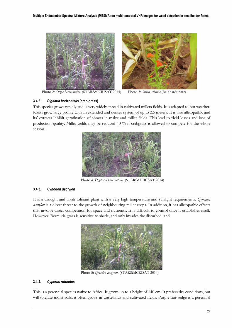
Multiple Endmember Spectral Mixture Analysis (MESMA) on multi-temporal VHR images for weed detection in smallholder farms.
27
Photo 2: Striga hermonthica. (STARS&ICRISAT 2014) Photo 3: Striga asiatica (Reinhardt 2012)
3.4.2. Digitaria horizontalis (crab-grass)
This species grows rapidly and is very widely spread in cultivated millets fields. It is adapted to hot weather.
Roots grow large profile with an extended and denser system of up to 2.5 meters. It is also allelopathic and
its’ extracts inhibit germination of shoots in maize and millet fields. This lead to yield losses and loss of
production quality. Millet yields may be reduced 40 % if crabgrass is allowed to compete for the whole
season.
Photo 4: Digitaria horizontalis. (STARS&ICRISAT 2014)
3.4.3. Cynodon dactylon
It is a drought and alkali tolerant plant with a very high temperature and sunlight requirements. Cynodon
dactylon is a direct threat to the growth of neighbouring millet crops. In addition, it has allelopathic effects
that involve direct competition for space and nutrients. It is difficult to control once it establishes itself.
However, Bermuda grass is sensitive to shade, and only invades the disturbed land.
Photo 5: Cynodon dactylon. (STARS&ICRISAT 2014)
3.4.4. Cyperus rotundus
This is a perennial species native to Africa. It grows up to a height of 140 cm. It prefers dry conditions, but
will tolerate moist soils, it often grows in wastelands and cultivated fields. Purple nut-sedge is a perennial

Multiple Endmember Spectral Mixture Analysis (MESMA) on multi-temporal VHR images for weed detection in smallholder farms.
28
weed that has serious impacts on agriculture. Although relatively small in stature, it highly competes for
water and nutrients. It grows very fast forming dense colonies by producing an extensive system of rhizomes
and tubers causing a reduction in crop yields.
Photo 6: Cyperus rotundus. (Extension 2015)
3.4.5. Echinochloa colona
It is a fast growing and notorious weed but does not tolerate drought. This grass may become a nuisance to
farmers. When left uncontrolled in millet fields or orchards, it can form a very dense vegetative growth that
will compete with the crop for water and nutrients.
Photo 7: Echinochloa colona. (STARS&ICRISAT 2014)
3.4.6. Rottboellia cochinchinensis
This is an aggressive weed and is on the list of weeds for the Federal Noxious Weed Act. In Mali, it is
prominent in open, well-drained places at higher altitudes, and is one of the important species in old field
succession. It causes severe crop damage to millet and corn. It is also an alternate host of the viruses causing
corn leaf gall.
Photo 8: Rottboellia cochinchinensis. (STARS&ICRISAT 2014)

Multiple Endmember Spectral Mixture Analysis (MESMA) on multi-temporal VHR images for weed detection in smallholder farms.
29
3.4.7. Commelina forskalaei
This species is herbaceous plant native Africa. It can be easily recognized by its bright blue flowers with
winged stamen filaments. It forms dense mats, and can be found most commonly in sandy soils in at least
somewhat sunny situations.
Photo 9: Commelina forskalaei. (STARS&ICRISAT 2014)
3.4.8. Cenchrus biflorus
It is an annual grass found in the Sahel countries. It is usually referred to as "cram-cram". It is also either alone or mixed with millet. Cenchrus biflorus is regarded as a noxious weed because of its spreads rapidly.
Photo 10: Cenchrus biflorus. (STARS&ICRISAT 2014)
3.4.9. Amaranthus viridis,
This is a broad-leaved weed found in maize and millet. A. viridis is very common weed in maize fields most
especially during the early growing stages of a crop. The slender amaranth is considered as one of the most
harmful weeds which may lead to heavy losses in crop yield. Its weedy status is more important than its
culinary value. It is eaten as a vegetable.
Photo 11: Amaranthus viridis. (cabi 2015)

Multiple Endmember Spectral Mixture Analysis (MESMA) on multi-temporal VHR images for weed detection in smallholder farms.
30
3.4.10. Imperata cylindrica
This is the worst weed of the moist savanna in West Africa. According to (Chikoye et al., 2002; Chikoye et
al., 2014), it is the tenth most infamous weed species in the world, which affects farmers who practice slash-
and-burn agriculture (Holm et al. 1979). It is noxious because of its wide distribution and adapted to a wide
range of climatic conditions and soils. It is highly competitive with many crops including millet and corn
and it is resistant to control. It causes yield reductions of 51- 62 % in millet when the crop is weeded 2-4
times.
Photo 12: Imperata cylindrica. (STARS&ICRISAT 2014)
According to Chikoye et al. (2014), the perennial weeds like Cyperus rotundus, Cynodon dactylon and Striga are
among the worst weeds of the world, infest the millet crop reducing greatly the millet production and quality.
3.4.11. Sonchus oleraceus (sow-thistle)
S.oleraceus has been widely dispersed deliberately or accidentally by humans. It invades mainly open and disturbed areas/cultivated land/ gardens. It grows rapidly once introduced.
Photo 13: Sonchus oleraceus. (STARS&ICRISAT 2014)

Multiple Endmember Spectral Mixture Analysis (MESMA) on multi-temporal VHR images for weed detection in smallholder farms.
31
4.0 METHODOLOGY
4.1. Introduction to methodology
This chapter provides the strategies or methods that are used in this study in order to achieve its objectives.
The selection of the method is based on a thorough literature review as explained back in chapter 2. Data
preparation, spectral mixture analysis, temporal analysis of the WV-2 images using vegetation indices, the
class separability techniques and accuracy assessments are explained.
4.2. Data preparation and preprocessing
Data provided by the STARS projects was sorted, organized and focused on a millet field in Soughoumba.
The data was sorted at a quadrat level (2 m × 2 m), plot level (15 m × 15 m) (see Chapter 3) and the entire
field as shown in Figure 4.1. The remote sensing data comprised of multi-temporal WV-2 images with a
spatial resolution of 2 meters. Geometric corrections and radiometric corrections were applied to the earth
observation data before these could be used for processing and analysis.
Figure 4.1: Plots and quadrats distribution in the crop field. The letter A-F refers to the plots while the number refers
to the quadrat. The dots refer to the spatial location of the quadrat

Multiple Endmember Spectral Mixture Analysis (MESMA) on multi-temporal VHR images for weed detection in smallholder farms.
32
4.2.1. Image preprocessing
4.2.1.1. Correction for radiometric, atmospheric effects and ortho-rectification
In this research, WV-2 images were corrected for radiometric and atmospheric effects, BRDF effects, as
well as Ortho-rectification. These corrections were performed the by the STARS project. Radiometric
corrections were done to correct for the sensitivity of the sensor to the objects through calibration so as to
convert at-sensor radiance to apparent at-sensor spectral reflectance required before atmospheric correction.
This is usually done taking into account temporal changes in solar illumination due to Earth-Sun angle.
The radiation movement through a medium is affected by absorption, emission and the scattering processes.
A surface reflectance signal that is measured by passive satellite instruments is contaminated by the influence
of the atmosphere. The atmospheric correction involves the removal of this contamination. In this research,
the atmospheric correction was done using the Simulation of a Satellite Signal in the Solar Spectrum radiative
transfer model (6S) that was specifically adjusted for the Digital Globe, Worldview (WV) dataset for the
STARS-project. This model uses the external information derived from moderate Resolution Imaging
Spectro-radiometer (MODIS) for aerosol and atmospheric effects estimation on the day of image
acquisition.
Satellite images data are usually affected by the systematic sensor and platform-induced geometry errors.
There exist topographical variations on the earth’ surface. A sensor tilt affects the distance with which
features on the satellite are displayed. A more varied topography leads to more distortions on the image. In
this research, the image used were orthorectified to correct for the tilt distortions using a digital elevation
model (DEM).
4.2.1.2. Image registration
Image registration geometrically aligns two images of the same scene with different a viewing geometry
and/or different terrain distortions into the same coordinate system so that corresponding pixels represent
the same objects. All the 7 images were captured at different times or/and from different viewpoints causing
the images to be miss-aligned. 100 tie points were automatically generated. Tie points with high RMS error
were deleted. The resulting accuracy was below RMS of 0.57 for all the image date. This process was repeated
in all the bands. The tie points were used to compute the geometric transformations of the warped image
thereby aligning the warped image to match the base image. This was successfully done using the image to
image registration in ENVI/IDL.
4.2.1.3. Creating a crop-specific mask
It is necessary to first identify the target crop field in the scene. Seven WV-2 cloudless images comprising
of all the 3 fields were selected from the STARS project database to provide the necessary information that
captures the target crop phenology. The field and plots boundaries were visually checked whether they
matched with the image. A slight shift was observed, the shift parameters were estimated as follows: Polygon
coordinates x: a shift by 6 pixels to the left (West), Polygon coordinates y: a shift by 2 pixels up (North).
This shift was corrected for using the shift parameters to alight the field boundary to the images. The images
were masked using the field boundary shapefiles. The field boundaries used were recorded in the field with
a Trimble JUNO GPS without any differential correction. The typical accuracy of the boundary position is
5 to 10 meters. A total of 21 image subsets were created.

Multiple Endmember Spectral Mixture Analysis (MESMA) on multi-temporal VHR images for weed detection in smallholder farms.
33
4.3. Vegetation indices analysis
Based on their spectral characteristics, various vegetation indices were selected and computed. The mean
values of the vegetation indices were extracted from the images. The Table 4.1 below shows the indices
used for this study and their formula.
Table 4.1: The formulae for computation of the vegetation indices
Vegetation index Formula Author
Normalized Difference Vegetation
Index (NDVI)
Modified Soil Adjusted Vegetation
Index (MSAVI2)
Soil and Atmospherically Resistant
Vegetation Index (SARVI)
Renormalized difference vegetation
index (RDVI)
Transformed Difference Vegetation Index (TDVI) World-View improved vegetative index (WV-VI)
Modified triangular vegetation index
(MTV12)
(NIR – R) / (NIR + R)
[2 × NIR + 1 – sqrt ((2 × NIR + 1) ^ 2 –
8 × (NIR – R))] / 2
[(NIR - RB) × (1+ L) / (NIR + RB + L)]
L is a canopy adjustment factor ,
RB = R - gamma × (B-R)
(NIR - R) / sqrt(NIR + R)
sqrt [(NIR-R)/(NIR+R)+0.5)]
(NIR2 – R) / (NIR2 + R)
1.5 [1.2 × R800 - R550) - 2.5 × (R670 - R550)]
/ [sqrt (2 × R800 + 1 ^ 2 – 6 × R800 – 5
× sqrt (R670) - 0.5)]
(Rouse et al.,1973)
(Qi et al., 1994)
(Kaufman and Tanre 1992)
(Roujean and Breon 1995)
(Bannari et al., 2002) (Wolf 2012)
(Haboudane et al. 2002)
Figure 4.2 shows the workflow of the VI extraction and analysis. The Vis were calculated and their means
recorded. The means were regressed against the Fcover in a regression analysis to determine the VI
which correlates well with the Fcover.

Multiple Endmember Spectral Mixture Analysis (MESMA) on multi-temporal VHR images for weed detection in smallholder farms.
34
Figure 4.2: The analysis procedure of VIs mapping with high-resolution WV-2 imagery
Spatial analysis was employed in order to evaluate the relationship between the ground reference Fcover in
and remotely sensed VIs. A linear regression analysis has been used in previous studies(Chapter 2) to show
the relationship between VIs and above ground biomass of different dates, however since the above ground
biomass was measured once in the field, the Fcover (the total green cover including crops and weeds) was
used instead. This was because Fcover was measured at different times that very closely corresponded to
the growth period and image acquisition date and therefore, gave high correlation with the VIs. Weeds and
crops occur in a mixture, therefore the subpixel classification as explained in the previous chapters, is
adopted estimate the weed, soil and crop fractions.
4.4. Spectral mixture analysis
4.4.1. Multiple endmember spectral mixture analysis (MESMA)
As opposed to simple linear spectral mixture analysis, MESMA allows for the number and types of
endmembers to vary per pixel. MESMA incorporates various constraints such as a minimum fit of the
model, the fraction, RMSE and residual constraints to test multiple models/endmembers for each image
pixel. A four endmember model was used to model the multi-temporal images. Both image and reference
endmembers were included in the multispectral library.
Reference endmembers were derived from the WV-VI images based on the field data collected and provided
by the STARS project. The field data included the weed proportions that were recorded in the fields. The
second set of endmembers was derived automatically from the image (image endmembers). Image
endmembers could easily be obtained from a satellite image. For this advantage, image endmembers were
preferred for this study. The procedure for MESMA un-mixing is described below.

Multiple Endmember Spectral Mixture Analysis (MESMA) on multi-temporal VHR images for weed detection in smallholder farms.
35
4.4.1.1. Endmember extraction
For automatic endmember extraction, the Pixel Purity Index (PPI) (Valdiviezo-N and Urcid 2012) was first
applied resulting to only one endmember (one pixel) that could be identified as pure after 50,000 iterations
therefore this method was disregarded. The Sequential Maximum Angle Convex Cone (SMACC)(Gruninger
et al., 2004) which extracts spectral endmembers throughout an image was used for this study. Compared
to PPI, this technique was less time consuming and not bounded by the number of bands.
4.4.1.2. Endmember extraction using SMACC
Representative pure spectral endmembers were extracted automatically in spectral un-mixing results using
of the sequential maximum angle convex cone (SMACC) algorithm in all the fields and across all the dates
to create spectral signatures and abundance images. The algorithm works by selecting the endmembers
directly from the image sequentially. The convex cone model finds a single endmember and increases as the
image dimension increases, new endmembers are identified based on the angles they form with an existing
cone. The following flow chart shows the process used in endmember extraction;
Figure 4.3: The endmember estimation and extraction process
The SMACC procedure was carried out on the July 29th, September 29th, October 10th, October 18th,
November 1st and November 14th, WV-2 multispectral images. The preference to this method was that it is
not bounded by the number of bands therefore, the number of endmembers selected could be more than
the number of bands.
4.4.1.3. Reference data
The reference data on the dominant cover in a crop field that was used in this study was collected from the
field and also visually derived from the ground photographs. The patches of dominant cover per pixel and
their relative composition were recorded per quadrat (2 m × 2 m) which is the size of 1 pixel of the WV-2
images being used in this study. Patches having over 75 % single species composition were recorded as pure.

Multiple Endmember Spectral Mixture Analysis (MESMA) on multi-temporal VHR images for weed detection in smallholder farms.
36
4.4.1.4. Creation of a spectral library for the reference data
Spectral library development and processing was done using the ENVI/IDL (ITT Visual Information
Solutions) image processing software. The spectra within the reference field boundary were extracted from
each image separately to a spectral library. All the duplicates were checked and removed from the single date
spectra.
4.4.1.5. Spectral matching
A quantitative comparison of the surface reflectance of the known endmembers with unknown
endmembers derived automatically using Spectral Angle Measure (SAM) (Kruse et al.,1993), a spectral
matching technique to identify the endmember spectral similarity. The SAM algorithm was implemented in
ENVI/IDL, it computed the angular distance between each unknown spectrum from the image end-
members and the reference spectra, and this resulted in an image that showed the best SAM match at each
pixel. The spectra with smaller angles (spectra that are close to the reference spectrum) were represented
with darker pixels. The dark spectrum (black/0 radians) represented a perfect match with the reference
spectrum.
4.4.1.6. Creation of the Metadata for the unknown endmembers
Several components of the MESMA classification technique required the spectra in a library to have
associated metadata. The metadata facilitated keeping of track of the class of each spectrum. The metadata
of each single date spectral library consisting of crop, weed and soil classes were created to enable the user
to identify the fractional classes and to select different criteria for sorting and viewing. All the spectra were
grouped into weed, soil and crop classes for all the fields and in all the dates.
4.4.1.7. Creation of a square array
Square arrays are images of the dimension are n by n, where n is the number of spectra in the library as
explained in. The array comprised of the RMSE, spectral angle, Endmember fraction and a shade fraction.
The shade endmember accounted for the brightness variations caused by shadowing and illumination
effects. Partially constrained mode (see chapter 2) was useful for allowing models with very good fit to be
included. Default parameters used for the creation of the square array were -0.05, 1.05 and 0.025 for a
minimum fraction, maximum fraction and RMSE threshold, respectively.
4.4.1.8. Computation of EAR and MASA and the selection of the optimal endmembers
The key to MESMA is to detect which spectra in a group of spectra are the best representative of a class
they represent while covering the range of variability within the class. The square array results were used
for the computation of the Endmember Average Root mean square error (EAR) (Dennison & Roberts,
2003a) and the Minimum Average Spectral Angle (Dennison et al., (2004). EAR selected the endmembers
with the lowest RMSE while the (MASA) selected the endmembers that had the lowest spectral angle
between to spectra. At least 4 spectra were selected for each class using both techniques. In this process, all
the endmembers were grouped into three cover classes, weed, crop and soil. The selected endmembers were
used to model the WV-2 images.

Multiple Endmember Spectral Mixture Analysis (MESMA) on multi-temporal VHR images for weed detection in smallholder farms.
37
4.4.1.9. Development of endmember models
Endmember variability is important. However, selecting the smallest optimal subset of available endmember
was equally important. A smaller representative set of endmembers was used for computational efficiency.
By varying the number of the selected spectra from each spectral library, different sets of cover fraction
were derived. Adequate fraction images and values were selected based on the percentage of pixels modelled.
A four endmember model (crop, weed, soil and shadow endmembers) was used to map the WV-2 images
using MESMA.
4.4.1.10. MESMA unmixing and classification
WV-2 images were unmixed into four fraction images comprising of soil, weed, crop and shade using
Multiple Endmember Spectral Mixture Analysis (MESMA). This technique decomposed each pixel using
different combinations of potential endmembers. A four- endmember model was used to unmix each pixel
is an image. MESMA package (source code can be found at (http://www.vipertools.org) was run in
ENVI/IDL to unmix the WV-2 images using a single date selected spectra per image. The following
constraints were set during the classification; Non-shade fractions were constrained to between −6 % and
106 %, a shadow of 0.8 %, RMSE was set at 2.5 % of the reflectance and the residuals were limited to 2.5
% for more than seven contiguous bands. Over 85 % of the pixels in all the images were modelled across
all the fields. The selection of the number and type of spectra used in each spectral library and unmixing of
the images were repeated till the resulting fraction images could allow an accurate estimate through a visual
comparison with the WV-VI and the field photographs. The spectra were also refined when the percentage
of classified pixels was as low as 60 for some images such as the September 29th and July 29th dates. New
spectra were introduced in order to redefine the training endmembers for these images. To effectively
classify the image, more weed endmembers were used as compared to crop endmembers because of the
diversity in the weed species.
4.4.2. Simple Linear Spectral Mixture Analysis
4.4.2.1. Selection of the model
Selecting endmembers involved identifying both the number and the type of endmembers and their
corresponding spectral signatures. As discussed previously, comparative studies have been undertaken to
determine the type of model that best fit the data for the spectral un-mixing algorithm. A linear model has
reliably been used to un-mix the proportion of fraction cover in a pixel due to its robustness and simplicity
in implementation as opposed to the complex non-linear/geometric models. Four endmembers (crop,
weeds and soil and automatically added shadow endmember) models were applied per field and per image
date.
4.4.2.2. Endmember extraction and spectral matching
Representative spectral were extracted automatically using the Sequential Maximum Angle Convex Cone
(SMACC) algorithm. The procedure was carried out for the July 29th, September 29th, October 10th, October
18th, and November 1st, November 14th WV-2 multispectral images resulting into 4 endmembers
representing 4 classes.

Multiple Endmember Spectral Mixture Analysis (MESMA) on multi-temporal VHR images for weed detection in smallholder farms.
38
4.4.2.3. Linear un-mixing
Spectral un-mixing was done to derive the proportions of each endmember for the SLSMA. The pixel
abundances were computed by constrained linear spectral un-mixing. The abundances were constrained to
be positive and were restricted to sum to 1. Simple linear spectral un-mixing yielded a series of abundance
maps, which represented proportions of each of the endmembers present in each pixel of the input image.
Linear un-mixing results also included a root-mean-square error (RMSE) image along with the abundance
maps and the spectral signatures. This RMSE image was as a result of the difference between the observed
pixel spectrum and the spectrum reconstructed from the calculated abundances. The RMSE error image
was used to identify the poorly defined classes.
4.5. Endmember separability
The spectral separability between the weeds and the crop endmembers was evaluated using Jeffrey’s Matusita
distance (JM) (Swain et al., 1978) and the Transformed Divergence measures (TD) (Jensen 1996). Signature
separability was calculated as the statistical difference between pairs of spectral endmembers. Crops and
weed endmembers derived using MESMA (EAR and MASA-selected endmembers) and those of Simple
Linear Unmixing were subjected to two quantitative tests for the separability analysis.
4.5.1. Transformed divergence (TD)
Computing transformed divergence was done using the following equations; Source: (Swain et al., 1978).
Where: i and j: are the endmembers being compared, Ci: is the covariance matrix of the endmember I, μi is
the mean vector of the endmember I, tr represents the trace function (matrix algebra) and T is the
transposition function.
4.5.2. Jeffries Matusita (JM).
Where: i and j are two classes being compared, Ci is the covariance matrix, mi is the mean vector, ln is the
natural logarithm function and |Ci| is the determinant of Ci (matrix algebra). Source: (Swain et al., 1978)
Eq. 7
Eq. 8
Eq. 9
Eq. 10

Multiple Endmember Spectral Mixture Analysis (MESMA) on multi-temporal VHR images for weed detection in smallholder farms.
39
Flow chart of the methodology adopted
Figure 4.4: The flowchart showing the spectral mixture analysis

Multiple Endmember Spectral Mixture Analysis (MESMA) on multi-temporal VHR images for weed detection in smallholder farms.
40
4.6. Accuracy assessment
The accuracy assessment was done to compare the accuracy of the modelled weed fraction as compared
with the reference fraction to quantitatively evaluate the model results. This was done using the coefficient
of determination (R2), the root mean squared error (RMSE), and the systematic error (SE) applied in Wu &
Yuan, (2007). These accuracy assessment measures were computed using the following equations. Source:
(Wu and Yuan 2007)
Where is the modelled fractional value of weed measured at sample i. Ii is the reference weed fraction
value, and I is the mean weed fraction of the samples and N is the total number of samples. The RMSE is
a measure of the overall estimation accuracy, and the SE is a measure of systematic errors such as
overestimation or underestimation (Wu 2004). The coefficient of determination is a measure similarity.
Eq. 11
Eq. 12
Eq. 13

Multiple Endmember Spectral Mixture Analysis (MESMA) on multi-temporal VHR images for weed detection in smallholder farms.
41
5.0 RESULTS AND DISCUSSION
5.1. Results
5.1.1. What is the relationship between the Fcover and vegetation indices?
Various spectral vegetation indices (VI) that are known to react to changes in vegetation vigour or variation
in chlorophyll content were compiled from literature. The indices were calculated from reflectance
measurements of cotton (27), millet (26) and maize (2). Seven vegetation indices were computed. All the
indices were normalized to a range between 0 and 1 to facilitate comparisons. The mean vegetation index
values and the standard deviation of all seven images are shown in Table 5.1.
Table 5.1: Mean of vegetation indices MSAVI2, MTVI2, NDVI, SARVI, TNDVI and WV-VI per image date and their standard deviations for the cotton (27), millet (26) and maize (2) fields.
Field Date
Index
F27
MSAVI2 STD MTVI2 STD NDVI STD RDVI STD SARVI STD TNDVI STD WV_VI STD
177 0.20 0.09 0.04 0.03 0.14 0.01 0.38 0.22 0.11 0.05 0.16 0.09 0.16 0.01
210 0.55 0.06 0.45 0.03 0.49 0.11 0.58 0.26 0.39 0.05 0.50 0.06 0.54 0.10
272 0.75 0.07 0.72 0.05 0.87 0.04 0.46 0.25 0.78 0.08 0.70 0.07 0.87 0.04
283 0.74 0.05 0.69 0.03 0.82 0.04 0.59 0.16 0.79 0.03 0.79 0.05 0.86 0.04
291 0.73 0.03 0.67 0.06 0.78 0.05 0.46 0.05 0.80 0.09 0.76 0.03 0.77 0.04
305 0.67 0.03 0.59 0.07 0.68 0.06 0.41 0.04 0.67 0.02 0.63 0.07 0.67 0.05
318 0.60 0.08 0.48 0.07 0.57 0.07 0.46 0.05 0.50 0.06 0.48 0.08 0.62 0.06
F26
177 0.31 0.03 0.13 0.04 0.23 0.05 0.21 0.03 0.17 0.02 0.39 0.04 0.22 0.02
210 0.62 0.10 0.51 0.10 0.46 0.04 0.42 0.02 0.36 0.05 0.43 0.07 0.42 0.03
272 0.76 0.05 0.69 0.06 0.62 0.07 0.39 0.01 0.70 0.04 0.45 0.03 0.63 0.06
283 0.67 0.05 0.56 0.07 0.51 0.06 0.33 0.01 0.48 0.02 0.36 0.03 0.53 0.06
291 0.54 0.02 0.42 0.01 0.46 0.07 0.34 0.02 0.35 0.02 0.31 0.01 0.48 0.06
305 0.41 0.02 0.23 0.02 0.32 0.05 0.17 0.04 0.18 0.02 0.35 0.02 0.31 0.06
318 0.38 0.05 0.17 0.02 0.28 0.05 0.16 0.01 0.13 0.01 0.18 0.06 0.33 0.05
F2
177 0.24 0.02 0.05 0.01 0.23 0.07 0.12 0.01 0.04 0.01 0.12 0.04 0.24 0.03
210 0.59 0.02 0.44 0.04 0.43 0.02 0.34 0.02 0.34 0.02 0.17 0.02 0.43 0.04
272 0.84 0.05 0.79 0.06 0.74 0.07 0.29 0.04 0.94 0.05 0.37 0.03 0.75 0.02
283 0.73 0.06 0.63 0.07 0.59 0.08 0.43 0.04 0.64 0.03 0.75 0.02 0.61 0.07
291 0.42 0.03 0.33 0.07 0.50 0.05 0.25 0.06 0.31 0.02 0.65 0.07 0.52 0.06
305 0.34 0.03 0.22 0.01 0.37 0.02 0.20 0.06 0.18 0.05 0.24 0.02 0.39 0.02
318 0.31 0.01 0.18 0.01 0.33 0.09 0.18 0.06 0.13 0.01 0.25 0.06 0.37 0.06
Table 5.1 shows the Mean VI values and standard deviation values extracted from the WV-2 image acquired
at the near-nadir view. The VI values were extracted from the whole field and are associated with three
different crops (Cotton, weed and maize crop fields). The vegetation indices indicate the total vegetation
cover in the crop fields i.e. both weeds and the crop. Below are vegetation index profiles derived from the
VI Table 5.1.

Multiple Endmember Spectral Mixture Analysis (MESMA) on multi-temporal VHR images for weed detection in smallholder farms.
42
Figure 5.1: Mean of vegetation indices MSAVI2, MTVI2, NDVI, SARVI, TNDVI and WV-VI temporal profiles per image date and their standard deviations for the cotton (27), millet (26) and maize (2) fields.

Multiple Endmember Spectral Mixture Analysis (MESMA) on multi-temporal VHR images for weed detection in smallholder farms.
43
The VIs profiles in figure 5.1 show low values in June due to lack of green cover during field preparations
and sowing. The VI values increase rapidly from July to September except for the RDVI and the TNDVI
in September. This is the time the maize and millet were expected to start developing the vegetative material.
The maximum VI was reached on September 29th for all the three crop fields. On October 10th, the VI
started to decrease gradually onwards to the following days. The change in vegetation development in the
period on July 29th to September 29th was quite significant. In cotton, maize and millet fields, SARVI,
MSAVI2 and SARVI respectively, had the highest VIs peaks. The high values of MSAVI2 index result from
the fact that the constant value of 1.0 instead of 0.5 was included in the formula. A similar situation was
observed for all the crops with very slight changes.
5.1.2. Which VI is best suited for the crop field vegetation mapping using correlation analyses
The establishment of a relationship between NDVI and vegetation fraction cover (Fcover) based on the
change of NDVI during different temporal periods is important in crop and weed mapping. All the
computed vegetation indices were correlated with the Fcover. A regression analysis using R software (R
Core team 2013) was conducted using gstat package (Pebesma 2004) between the Fcover and vegetation
indices. The model that had the highest correlation coefficients was selected for modelling the relationship
between leaf chlorophyll content and vegetation indices. The results of the correlation analysis are listed in
Table 5.2.
Table 5.2: The Relationship between Fcover and VIs in the three fields. The relationships exhibit significant correlations.
Index
VI_ Fcover correlation (r2)
September 29th
Cotton Millet Maize
NDVI 0.75 0.75 0.79
MSAVI2 0.78 0.76 0.75
MTVI2 0.74 0.78 0.79
RDVI 0.79 0.73 0.76
TNDVI 0.76 0.78 0.79
SARVI 0.88 0.85 0.82
WV-VI 0.92 0.89 0.84
Figure 5.2 shows the correlation between some selected vegetation indices and the Fcover for field 27
(cotton field). A positive correlation is observed.

Multiple Endmember Spectral Mixture Analysis (MESMA) on multi-temporal VHR images for weed detection in smallholder farms.
44
Figure 5.2: Scatter plots showing the relationship between the Fcover and vegetation indices (NDVI, MSAVI2 and WV-VI) for the cotton field in September 29th.
The indices for correlation with Fcover values were NDVI (r2=0.75), MSAVI2 (r2=0.78), MTVI2 (r2=0.74),
RDVI (r2=0.79), TNDVI (r2=0.76), SARVI (r2=0.88) and WV-VI (r2=0.92) for the cotton field. The indices
for correlation with Fcover values were NDVI (r2=0.75), MSAVI2 (r2=0.76), MTVI2 (r2=0.78), RDVI
(r2=0.73), TNDVI (r2=0.78), SARVI (r2=0.85) and WV-VI (r2=0.89) for the millet field and the indices for
correlation with Cover values were NDVI (r2.0.80), MSAVI2 (r2=0.75), MTVI2 (r2=0.79), RDVI (r2=0.76),
TNDVI (r2=0.79) SARVI (r2 =0.82) and WV-VI (r2=0.84) for the maize field.
Figure 5.3 shows the temporal profiles of the WV-VI for the Cotton, Millet and the maize fields.
Figure 5.3: WV-VI profiles for the cotton, maize and millet crop fields.

Multiple Endmember Spectral Mixture Analysis (MESMA) on multi-temporal VHR images for weed detection in smallholder farms.
45
The green vigor started to reduce sharply between September 29th and October 10 for the maize and millet
fields and then gradually for the following dates. In cotton fields, the reduction in green vigor was gradual
through. As shown in the above profiles, most indices had a similar shape except for the RDVI and the
TNDVI which shows uniqueness in all the fields. The WV-VI for the three fields is visualized in Figures
5.3 - 5.6.
5.1.3. Vegetation index images
A threshold of <0.2 was applied to the NDVI images to separate the soil from the vegetation as in (Peña et
al., 2013)
a) WV-VI for the cotton field
Figure 5.4: The WV-VI for the July 29th, October 18th, November 1st and November 14th for the cotton field

Multiple Endmember Spectral Mixture Analysis (MESMA) on multi-temporal VHR images for weed detection in smallholder farms.
46
b) WV-VI for the maize field
Figure 5.5: WV-VI for the July 29th, October 18th and November 14th for the maize field.
c) WV-VI for the millet field
Figure 5.6: The WV-VI for the July 29th, October 18th and November 14th for the millet field

Multiple Endmember Spectral Mixture Analysis (MESMA) on multi-temporal VHR images for weed detection in smallholder farms.
47
WV-VI, which yielded r2=0.92 in Field 27, r2=0.84 in Field 26 and r2=0.84 in Field 2. Similarly, across all
fields, index WV-VI was more highly correlated with Fcover than any other therefore, was selected as the
most suitable VI for crop field mapping. This WV-VI was closely followed by SARVI which is less sensitive
to soil background effects and variations in Fcover. This WV-VI is selected for further comparison with
the spectral un-mixing classification results. The differences in the Vis per image date are attributed to the
changes in vegetation cover during the crop phenological cycle as shown in Photo 14.
Photo 14: Cotton field between July and November 2014 showing changes in temporal changes in vegetation cover (STARS&ICRISAT 2014)
5.2. Spectral mixture analysis
5.2.1. Results of Simple Linear Spectral Mixture Analysis (SLSMA)
One endmember per class (crop, weed, soil) was used to model the image and the results of the un-mixing
shadow normalized results are as shown in Table 5.3;
Table 5.3: Shade Normalized simple linear un-mixing weed, crop and soil fractions

Multiple Endmember Spectral Mixture Analysis (MESMA) on multi-temporal VHR images for weed detection in smallholder farms.
48
The model was constrained to sum to one and positivity endmember abundances. Table 5.3 shows the weed, crop and the soil abundances for the three study fields using simple linear spectral un-mixing. The following profiles in Figure 5.7 show the relationship between the weed and the crop fraction as observed in the three study fields.
Figure 3: Relation between the crop and weed fractions modelled using SLSMA

Multiple Endmember Spectral Mixture Analysis (MESMA) on multi-temporal VHR images for weed detection in smallholder farms.
49
In all the fields, a low weed fraction is modelled as compared to the crop fraction. The weed increases
when the crop started to dry off on October 18th and the following dates. This can also be observed in
the field data explained hereafter. The results obtained were compared with the MESMA fraction
estimates.
5.3. Multiple Endmember Spectral Mixture Analysis (MESMA)
5.3.1. Endmember extraction using SMACC
The results of this process were an abundance map, the regions of interest (this is the vector data that
contains mapping information of each endmember) and the extracted endmember spectra. Figure 5.8
illustrates the development of the maximum relative error in relation to the number of endmembers;
Figure 5.8: SMACC output: from left: A graph showing the behaviour of the maximum relative error (MRE) based on the number of endmembers in SMACC; (right) - Abundance map for Endmember 3 (September image) representing the cotton crop overlaid with the field boundary; spectral library plots (bottom).
The SMACC relative error tolerance was set at 0.01, relative error began to converge at endmember 7
markedly with additional endmembers. The number of endmembers extracted by SMACC algorithm was
user defined. A maximum of 30 endmembers as termination condition was chosen this was to allow more
endmembers per class required by MESMA un-mixing method in order to correct for within-class variation.
When the set number of endmembers was reached, the algorithm stopped. The abundance image represents
a crop endmember. The brighter value of the endmember signify a higher percentage and the darker values
shows a lower percentage of the endmember. Figure 5.9 shows spectral library plots extracted using the
SMACC technique.

Multiple Endmember Spectral Mixture Analysis (MESMA) on multi-temporal VHR images for weed detection in smallholder farms.
50
Spectral library plots for the cotton field (from left to right): September 29th, October 10th and October 18th
Spectral library plots for the Millet field: (from left to right): September 29th, October 10th and October 18th

Multiple Endmember Spectral Mixture Analysis (MESMA) on multi-temporal VHR images for weed detection in smallholder farms.
51
Spectral library plots for the maize field (from left to right): September 29th, October 10th and October 18th
Figure 5.9: Spectral library plots for the cotton, millet and maize fields. (From left to right): September 29th, October 10th and October 18th extracted using SMACC.
Above profiles are representative reflectance spectra derived from the WV-2 images using the SMACC
algorithm. The signatures show the pure spectral features found on the field. The endmember spectra show
some uniqueness especially in infrared bands for all the dates. The shape of the profiles changes with a

Multiple Endmember Spectral Mixture Analysis (MESMA) on multi-temporal VHR images for weed detection in smallholder farms.
52
change in time and the crop type. Figure 5.10 shows reference spectral profiles that were also derived from
the reference data and were used for the identification of the automatically generated spectra using spectral
matching.
Figure 5.10: The reference spectral libraries for the cotton millet and maize fields showing the spectra representing different weed infestation levels
5.3.2. Creation of the metadata files for the unknown endmembers
This metadata file created for the identified spectra. This file was stored in a comma separated value file
with the first column indicating the name of each spectrum and the associated x-y coordinates of the pixel
as shown in Table 5.4.

Multiple Endmember Spectral Mixture Analysis (MESMA) on multi-temporal VHR images for weed detection in smallholder farms.
53
Table 5.4: Metadata file for spectral library for the cotton field on September 29th
5.3.3. Square array results
The spectral angle image could be differentiated from the RMSE in that, the spectral angle was symmetrical
along the diagonal, signifying that the spectral angle was the same between two spectra. Figure 5.11 shows
the square array bands for the cotton field. The diagonal represents each spectrum modelling itself therefore,
its value is zero. Columns and rows store the model number, corresponding to one column and row for
each spectrum in the library. Each pixel corresponds to a column spectrum used to un-mix a row spectrum.
The EM fraction is the non-shade endmember. Usually, SMA fractions are between 0 and 100 %, and the
RMSE is calculated as the difference between the spectra of the brightness and the darker spectrum (chapter
3). The shade fraction was computed as 1 minus the EM fraction. The model was partially constrained and
was within the RMSE constraint.

Multiple Endmember Spectral Mixture Analysis (MESMA) on multi-temporal VHR images for weed detection in smallholder farms.
54
Figure 5.11: The partially constrained square array bands (from left to right): Shade fraction, RMSE band, EM fraction band, spectral angle band, and the Constraint-codes for all the image dates. (Table 5.5 below shows the mean values for the cotton field for the square array.
Table 5.5: Mean values for cotton field square array per image date
Band Mean values
29-Jul 29-Sep 10-Oct 18-Oct 1-Nov 14-Nov
RMSE 0.02 0.01 0.01 0.01 0.02 0.02
Spectral angle 0.09 0.06 0.05 0.06 0.09 0.09
EM- fraction 0.97 0.97 0.98 0.97 0.93 0.93
shade-fraction 0.01 0.02 0.01 0.02 0.06 0.05
constrained 0.85 0.78 0.81 0.68 0.74 0.69

Multiple Endmember Spectral Mixture Analysis (MESMA) on multi-temporal VHR images for weed detection in smallholder farms.
55
5.3.4. Selection of the optimal endmembers
The result of the Spectral array creation process was used for the computation of the EAR (RMSE) and
MASA (spectral angle) error metrics. The endmembers with the lowest spectral angle and the lowest RMSE
for were selected for the MESMA un-mixing process. The endmembers selected from the single-date spectra
to classify the single date image for the maize field (Field 2) are as shown in Table 5.6.
Table 5.6: The endmember selection by date for the cotton field.
EM-selection method Date
Class 29-Jul 29-Sep 10-Oct 18-Oct 1-Nov 14-Nov
Number of endmembers selected per date
MASA Crop 5 4 6 5 4 4
weed 7 8 7 6 4 4
Soil 4 3 3 4 5 6
EAR Crop 4 4 5 4 4 4
Weed 5 5 5 4 4 4
Soil 4 4 4 5 4 5
A higher number of endmembers was selected using the MASA endmember selection technique. Moreover,
more weed endmembers were selected by both methods as compared to the crop and soil classes. This was
also observed in the other fields.
5.3.5. What is the minimum class separability for the recognition of weed and the crop?
The class separability between weed and crop endmembers was evaluated using Transformed Divergence
(TD) and Jefferies-Matusita Distance (JM). The analysis of spectral separability using the TD and JM
measures showed a relatively similar pattern as observed in the Table 5.7 and 5.8 respectively, between weeds
and crop endmembers. The seperability analysis was done in all the three fields and all image dates. The
results shows that during the early crop growth stages of leave development, formation of side shoots, and
stem elongation in July through September and the late the crop development stage during ripening and
senescence (November), all the three crops have a better spectral separability as compared to the Middle
growth stage (October).
When analyzing the numerical TD values (Table 5.7) we can conclude that the separability values of the
MESMA representative spectra are good enough and the spectra are separable. However for the simple
linear un-mixing, the TD separability indices were relatively lower as observed visually in the figure 5.12-
5.13 for TD and 5.14 for JM respectively. The best average separability indices for the TD and JM values
for each date are shown. Class Separability values greater than 1850 for both the TD and JM were obtained
for the EAR and MASA for all the fields except for the October 10th in the cotton field. The values for the
JM distance for the data set (Table 5.8) are higher than those of JM across all the fields and image dates.

Multiple Endmember Spectral Mixture Analysis (MESMA) on multi-temporal VHR images for weed detection in smallholder farms.
56
Table 5.7: TD separability indices for the three fields using representative endmembers selected by various techniques. See Figure 5.11 for graphical representation.
Date Measure
Millet Field Maize field Cotton field
MASA EM
EAR EM
SLSMA EM
MASA
EM EAR EM
SLSMA EM
MASA
EM EAR EM
SLSMA EM
29-Jul TD 1835 1823 1724 1860 1855 1743 1845 1818 1724
29-Sep TD 1883 1876 1762 1929 1917 1826 1895 1884 1768
10-Oct TD 1817 1811 1681 1858 1835 1763 1820 1816 1712
18-Oct TD 1834 1822 1724 1864 1842 1787 1837 1823 1764
1-Nov TD 1913 1893 1797 1945 1940 1855 1912 1904 1824
14-Nov TD 1981 1957 1849 1977 1973 1897 1949 1939 1852
Figure 5.12: Graphical representation of TD separability indices between the 3 endmember selection methods per date for the millet and maize

Multiple Endmember Spectral Mixture Analysis (MESMA) on multi-temporal VHR images for weed detection in smallholder farms.
57
Figure 5.13: Graphical representation of TD separability indices between the 3 endmember selection methods per date for the cotton field.
Table 5.8: The JM separability indices for the three fields using representative endmembers selected by various
techniques. See Figure 5:13 for graphical representation
Date Measure
Millet Field Maize field Cotton field
MASA EMs
EAR EMs
SLSMA EMs
MASA EMs
EAR EMs
SLSMA EMs
MASA EMs
EAR EMs
SLSMA EMs
29-Jul JM 1975 1953 1774 1942 1913 1774 1872 1835 1707
29-Sep JM 1953 1944 1757 1914 1896 1792 1896 1873 1772
10-Oct JM 1849 1819 1641 1817 1806 1715 1812 1798 1701
18-Oct JM 1863 1852 1650 1862 1851 1741 1823 1805 1715
1-Nov JM 1969 1959 1797 1980 1945 1845 1898 1872 1770
14-Nov JM 1941 1927 1749 1947 1936 1834 1890 1874 1745

Multiple Endmember Spectral Mixture Analysis (MESMA) on multi-temporal VHR images for weed detection in smallholder farms.
58
Figure 5.14: Graphical representation of JM separability indices between the 3 endmember selection methods per date for the millet, maize and cotton field.

Multiple Endmember Spectral Mixture Analysis (MESMA) on multi-temporal VHR images for weed detection in smallholder farms.
59
Highly separable signatures signified better training spectra for the classification and vice versa. The MASA
endmembers separability indices for both the separability techniques showed a higher index than the EAR
endmembers separability indices. For simple linear spectral unmixing, the separability was very low which
indicated that there was much overlap between the weed and the crop spectra. The endmember separability
computed using SLSMA indicated a similar temporal pattern to that of EAR/MASA with higher values
during early and late stages of the crop development and lower in the mid- growth stages.
5.4. MESMA unmixing and the classification results
The selected spectra with the lowest EAR /MASA were grouped into different spectral libraries allowing us
to un-mix various models of four endmembers (weed, crop, soil and shade). Using the defined spectral
libraries, above 85 % of all the images met the 0.025 RMSE criterion. A three endmember model (crop,
weed and shadow) was first used for the un-mixing but almost 40 % of all the images was left un-modelled.
Upon the addition of a fourth endmember (soil), the percentage of the modelled pixels increased up to 85
% and above in all the images. Fraction images were constructed using the selected minimum EAR/MASA
endmembers. The modelled fractions were normalized by their corresponding shade fraction. Shade
normalization divided each non-shade fraction by the sum of all non-shade fractions producing uniform
normalized fractions of 100 %. The resulting fraction images and values were later used to investigate the
spatial pattern and distribution of the weed class as shown in Figures 5.15 - 5.18.
Weed fraction maps: cotton field
Figure 5.15: Weed fraction images per date for the cotton field modelled using EAR endmembers

Multiple Endmember Spectral Mixture Analysis (MESMA) on multi-temporal VHR images for weed detection in smallholder farms.
60
Figure 5.16: Weed fraction images per date for the cotton field modelled using MASA endmembers
The weed fraction in each pixel is represented by a grey value. The brighter values represent the areas with
a high proportion of weed while the darker values signify areas with lower weed proportion. The shade
normalized EAR endmembers modelled results for the cotton field shown in Figure 5.15 indicate that in
July 29th weed proportions were high at the middle of the field. On September 29th, the weeds were more
evenly spread in the field similarly to October though there was a slight reduction weed proportion on
October 10th. The weed increased gradually through October 18th onwards. There is no suitable field data
for the October and July images, however, the field data shows increased weed fraction in September and
November and also based on the crop phenological cycle of the cotton crop. This presumably could be
attributed to the drying up of the crop paving the way for the weeds to grow. This pattern is also observed
in MASA endmembers estimated weed fraction.
Figure 5.17: Weed fraction images per date for the millet field modelled using MASA endmembers

Multiple Endmember Spectral Mixture Analysis (MESMA) on multi-temporal VHR images for weed detection in smallholder farms.
61
The shade normalized EAR-endmember estimated weed fractions for the millet field are not included in
Figure 5.17 but are include in Table 5.9. On July 29th, there was a high weed proportion and October 10th
has reduced weed proportion. Weeding data for this field were not available, however, the reduced weed
proportion was observed on September 29th. Presumable, this could be attributed to other forms of weeding
such as the use of herbicides or as a result of the canopy closure thereby suppressing the growth of weeds.
The weeds increased gradually on October 18th through November 1st and November 14th. This weed
increase could presumably be attributed to the drying up of the crop paving the way for the weeds to grow.
This also applied to the MASA weed fractions but with slight changes attributed to spectral modelling where
different endmembers are selected.
Weed fraction maps: Maize
Figure 5.18: Weed Fraction images per date for the maize field modelled using EAR endmembers (top image) and MASA endmembers (bottom image)

Multiple Endmember Spectral Mixture Analysis (MESMA) on multi-temporal VHR images for weed detection in smallholder farms.
62
The shade normalized EAR endmember estimated weed fractions for the maize field are shown in figure
5.18. The amount of weed fraction in each pixel is represented by a grey value. The brighter values represent
the areas with high weed proportion while the darker values signify areas with lower weed proportion.
Lower fractions of the weed class were observed in the November 14th image. This could be attributed to
crops and weeds drying up especially for the weeds that depend on the crop for development. Or due to a
dry period leading to reduced fractions for the shallow-rooted weeds. Similarly, the shade normalized MASA
endmember estimated weed fraction, increased weed proportion was observed on July 29th and September
29th. However weeds reduced rapidly on October 10th and could be attributed to weeding, two weeks later
on October 18th, weeds patches seemed to increase and the same case applied the following dates. The
results for the September image corresponds to the recorded field data weed fraction for the September 29th
was recorded to be between 10-50 %.
5.4.1. What is the weed infestation percentage in the crop fields?
For the best-fit model for each pixel, the fraction values for each endmember, and the identity of those
endmembers were recorded. The modelled fraction values for crop, weed and soil land cover classes as well
as their standard deviations are shown in Table 5.9.
Table 5.9: Shade Normalized unmixed crop, weed and soil cover classes per date using EAR and MASA-selected endmembers
Cotton field Millet field Maize field
Date Class EAR fraction
Std MASA fraction
Std EAR fraction
Std MASA fraction
Std EAR fraction
Std MASA fraction
Std
29-Jul weed 0.13 0.02 0.22 0.02 0.27 0.02 0.27 0.03 0.26 0.03 0.2 0.02
crop 0.56 0.02 0.51 0.02 0.34 0.02 0.35 0.02 0.46 0.07 0.49 0.02
soil 0.31 0.02 0.27 0.02 0.39 0.02 0.37 0.02 0.29 0.06 0.3 0.02
29-Sep
weed 0.30 0.01 0.34 0.03 0.11 0.06 0.12 0.01 0.19 0.04 0.17 0.02
crop 0.69 0.03 0.52 0.03 0.53 0.03 0.5 0.03 0.69 0.08 0.72 0.02
soil 0.19 0.01 0.14 0.05 0.36 0.04 0.39 0.03 0.12 0.06 0.11 0.1
10-Oct
weed 0.40 0.03 0.42 0.03 0.13 0.02 0.12 0.01 0.11 0.02 0.11 0.11
crop 0.58 0.03 0.65 0.03 0.65 0.02 0.65 0.04 0.67 0.02 0.7 0.24
soil 0.02 0.06 0.01 0.06 0.22 0.02 0.23 0.03 0.22 0.02 0.19 0.23
18-Oct
weed 0.09 0.08 0.13 0.07 0.15 0.02 0.1 0.02 0.24 0.02 0.32 0.03
crop 0.57 0.03 0.63 0.03 0.44 0.02 0.48 0.02 0.46 0.02 0.31 0.03
soil 0.33 0.03 0.25 0.03 0.41 0.09 0.41 0.01 0.3 0.02 0.37 0.02
1-Nov
weed 0.33 0.03 0.37 0.02 0.17 0.06 0.26 0.02 0.18 0.02 0.31 0.02
crop 0.20 0.08 0.23 0.01 0.35 0.08 0.33 0.02 0.34 0.02 0.31 0.08
soil 0.47 0.03 0.4 0.02 0.48 0.03 0.41 0.01 0.49 0.02 0.38 0.07
14-Nov
weed 0.36 0.02 0.28 0.02 0.31 0.05 0.34 0.01 0.16 0.02 0.19 0.02
crop 0.11 0.02 0.13 0.02 0.14 0.07 0.06 0.01 0.16 0.06 0.13 0.02
soil 0.53 0.02 0.59 0.02 0.55 0.08 0.6 0.01 0.68 0.08 0.68 0.19

Multiple Endmember Spectral Mixture Analysis (MESMA) on multi-temporal VHR images for weed detection in smallholder farms.
63
In Table 5.9, the sum of the fractions (weed, soil and crop) adds up to 1. Following the constraints imposed
on the un-mixing model. Differences could be observed between weed fractions unmixed using EAR and
MASA selected weed, soil and crop endmembers. The weed fraction for the cotton field was 0.13 for July
29th. The weed fraction increased rapidly to 0.30 on September 29th and further increased to 40 on October
10th. There was a rapid decrease to 0.09 on October 18th. The same trend was observed in the corresponding
MASA weed fractions but with a decrease on November 14th. According to the field data, this pattern was
also observed. The September field data had between 10-50 % weed proportions while the August image
had <10 % weed proportions. There was no suitable field data the July 29th, October 10, October 18 and
November 14 for accuracy assessment and comparison of the un-mixing results. However, to the authors
own assumption, the drying up of the crop in November would have led to the increased weed fraction due
to the open canopies (direct sunlight for weed development). The same pattern was also observed in the
field photographs as shown in Photo 15.
Photo 15: Cotton field between August and November 2014 showing different weed proportions.
(STARS&ICRISAT 2014)
For the millet field, the weed was high (0.27) on July 29th but this reduced on September 29th (0.11) with a
gradual increase on October 10th, October 18th and November 1st and a rapid increase on November 14th.
As the crop dried up, there was a gradual increase in weeds as observed in EAR fractions. The same trend
was observed in the corresponding MASA weed fractions but with a decrease on October 18th (0.10) and a
rapid increase in November 1st which is attributed to the drying up of the crop paving the way for the growth
of weeds. According to the field data, there was no suitable field data for July 29th, October 10, and October
18 and November 14. August field data was provided but there was no corresponding Satellite image for
this date. Ground reference data was provided for the August and September images data was provided but
no data was provided for the other dates. The majority of the quadrants were reported to having between
0-10 % weed fractions while some had between 10-50 % weed fractions. Photo 16 represent the field
photographs showing different weed proportions in the millet field.
August September 8th September 26th
Photo 16: Millet field between June and November 2014 showing different weed proportions. (STARS&ICRISAT
2014)
For the field 2, the weed was high (0.26) in the July 29th but this reduced on September 29th (0.19) with a
further decrease on October 10th (0.11). A rapid increment could be observed on October 18th (0.24) and a

Multiple Endmember Spectral Mixture Analysis (MESMA) on multi-temporal VHR images for weed detection in smallholder farms.
64
gradual reduction in November 1st (0.18) and November 14th (0.16) as observed in EAR fractions. The same
pattern is observed in the corresponding MASA weed fractions but with slight differences.
In the August field data majority of the quadrats were recorded having between 0-10 % weed fraction while
some had 10-50 % weed fractions similar to the September field data. On November 6th, most of the
quadrats were reported as having between 10-50 % weed fractions. This pattern is shown in Photo 17.
August 8th September-November 6th
Photo 17: Maize field between August and November 2014 showing different weed proportions.(STARS&ICRISAT 2014)
The un-mixing results were averaged per field, whereas the field data was provided per plot which was
further broken down into quadrats. When comparing the modelled weed fraction with the actual field data,
plot A was selected since it was set out as a farmer’s practice plot while the other plots (B, C, D and E) were
not included since they were fertilizer application trials. Plot A boundary and the quadrats were overlaid on the
modelled fraction image. The modelled image pixels values corresponding to the plot A quadrats values
were extracted using the Z profile in ENVI version 5.3 (Exelis Visual Information Solutions). A regression
analysis using R software (R Core team 2013) was conducted using gstat package (Pebesma 2004) between
the modelled weed fraction and the reference weed fraction.
5.4.2. What is the comparison of the modelled weed with the reference weed fraction?
Including several weed and crop endmembers appropriately not only represented the vegetation more
accurately but also gave us more confidence in the endmember choice. Thus, the ability to combine four-
endmember model resulted into a single image using simple selection criterion (EAR/MASA) greatly
enhanced our ability to correctly identify ground constituents.
Reference weed fractions were derived through the visual analysis of the ground photographs.
Photo 18: Millet field weed fraction estimation using field photographs. (STARS&ICRISAT 2014)
Evaluating vegetation fraction estimates are challenging due to the difficulty of obtaining reference data.
The lack of an accuracy assessment for three fraction images (July 29th, October 18th, and October 10th) was
a limitation of this study. The R-squared (R2), root mean square error (RMSE) and Standard error (SE) were
computed for the weed fraction images to compare the accuracy of the modelled fraction so as to
quantitatively evaluate the model results. The reference weed fraction was compared with the modelled
weed fractions using EAR/MASA results as well as the results derived from the Simple linear spectral
unmixing. The results were shown in the Figure 5.19.

Multiple Endmember Spectral Mixture Analysis (MESMA) on multi-temporal VHR images for weed detection in smallholder farms.
65
The accuracy of the methodology was evaluated by comparing the estimated weed coverage derived from
MESMA and simple linear spectral analysis with the values observed in the on-ground photographs and the
recorded weed fractions in the fields. The relationship between the estimated and observed weed densities
was satisfactory, the highest coefficient of determination for the cotton field was R2=0.722, RMSE=0.041
and an SE= 0.003 on September 29th while the lowest was on October 18th with an R2=0.591, RMSE=0.043
and SE= 0.001 for the MASA results. The highest coefficient of determination for the EAR weed fraction
was R2=0.717, RMSE=0.051 and an SE= 0.006 on September 29th and the lowest EAR fraction was
observed on October 18th an R2=0.566, RMSE=0.049 and SE= 0.006. For the SLSMA weed fraction
results, the highest coefficient of determination for the cotton field was R2=0.584, RMSE=0.058 and an
SE= 0.028 on September 29th while the lowest was recorded on October 18th with an R2=0.501,
RMSE=0.059 and SE= 0.024 were recorded. The MASA results showed a higher agreement as compared
to the corresponding EAR results across all the fields. Comparing the two SMA results, MESMA had a
higher R-Squared, lower standard error and lower RMSE. The results of the comparison are shown in Table
5.10. The results can be graphically visualized in Figure 5.19.
Table 5.10: Accuracy assessment of the modelled weed fraction with the reference weed data in all the image dates for the cotton, millet and the maize fields.
MESMA SLSMA
Field 27
Date MASA EAR Simple LSMA
R2 SE RMSE R2 SE RMSE R2 SE RMSE
29-Jul 0.651 0.003 0.041 0.646 0.003 0.046 0.531 0.016 0.062
29-Sep 0.722 0.001 0.048 0.717 0.006 0.051 0.584 0.028 0.058
10-Oct 0.618 0.003 0.047 0.634 0.005 0.053 0.523 0.027 0.069
18-Oct 0.591 0.001 0.043 0.566 0.006 0.049 0.501 0.024 0.059
1-Nov 0.654 0.012 0.035 0.645 0.001 0.046 0.562 0.023 0.056
14-Nov 0.678 0.003 0.042 0.653 0.005 0.057 0.574 0.021 0.068
Field 26 29-Jul 0.642 0.004 0.035 0.613 0.005 0.038 0.547 0.006 0.056
29-Sep 0.667 0.005 0.062 0.642 0.014 0.056 0.565 0.008 0.061
10-Oct 0.636 0.003 0.034 0.621 0.005 0.042 0.521 0.007 0.051
18-Oct 0.666 0.002 0.032 0.655 0.004 0.048 0.506 0.008 0.059
1-Nov 0.674 0.006 0.048 0.664 0.004 0.056 0.545 0.006 0.063
14-Nov 0.691 0.003 0.041 0.676 0.006 0.048 0.562 0.008 0.053
Field 2
29-Jul 0.646 0.001 0.026 0.625 0.001 0.033 0.542 0.004 0.041
29-Sep 0.673 0.006 0.056 0.631 0.003 0.056 0.524 0.007 0.062
10-Oct 0.646 0.006 0.046 0.621 0.003 0.053 0.506 0.007 0.058
18-Oct 0.665 0.008 0.049 0.642 0.007 0.056 0.531 0.008 0.068
1-Nov 0.674 0.003 0.032 0.647 0.003 0.039 0.565 0.009 0.048
14-Nov 0.708 0.005 0.036 0.685 0.006 0.038 0.584 0.006 0.049

Multiple Endmember Spectral Mixture Analysis (MESMA) on multi-temporal VHR images for weed detection in smallholder farms.
66
July 29th EAR-modelled fraction September 29th EAR-modelled fraction
October 18th EAR-modelled fraction November 14th EAR-modelled fraction
Figure 5.19: Scatterplots showing the relationship between the EAR-modelled weed fraction and the reference weed fraction for the cotton fields.
It was evident from that there was a positive relationship between the modelled WV-2 weed fraction and
the field data. The high R2, low RMSE and SE indicated that the pixels were well modelled as a linear
combination of the endmembers while the vice versa indicated that the linear combination of the
endmembers and the abundances did not match with the reference data. The low R2, high RMSE and SE
may be attributed to the wrong choice of the endmembers. Since field data collection date did not match
any image acquisition dates this may have greatly influenced the results. The July image accuracy assessment
was based august field data, the September 29th and October 10th was assessed using September 8th and 16th
field data. The November images were assessed using November 6th field data. All the image dates did not
match the field data collection dates.
5.4.3. What is the comparison between the EAR and MASA results?
Two techniques EAR and MASA were used to model combinations of spectra from the spectral library.
Each spectrum in a given class was used to model the members of the class. Four different types of
comparisons between EAR and MASA were investigated;
5.4.3.1. Comparison of the relationship between EAR and MASA weed un-mixing results against time
In this research, the general behaviour of temporal profiles of weed fraction values was obtained by applying
spectral un-mixing (MESMA and simple linear un-mixing (SLSMA) to multi-temporal WV-MS images.
When plotted against time, weed fraction modelled by the two endmember selection techniques showed a

Multiple Endmember Spectral Mixture Analysis (MESMA) on multi-temporal VHR images for weed detection in smallholder farms.
67
well-defined relationship with the crop phenological cycle. The multi-temporal profiles acquired for weed
using the MESMA approach are compared. A relationship between the EAR and MASA approaches is
shown in Figure 5.20
Figure 5.20: Relationship between EAR and MASA un-mixing weed fraction for the cotton (27), maize (2) and millet (26) with reference to time.

Multiple Endmember Spectral Mixture Analysis (MESMA) on multi-temporal VHR images for weed detection in smallholder farms.
68
In Figure 5.20, temporal profiles of the weed in maize and millet fields have a similar pattern starting with
a high value on July 29th, both with a peak on October 18th, a rapid reduction on November 1st and a gradual
reduction on November 14th. For field 26th, there is a reduced weed fraction on September 29th and for
field 26, the weed fraction decrease is observed on October 10. Also observed, the weed fraction modelled
by MASA is slightly higher than that of the EAR fraction. In Field 2, EAR weed fractions are higher than
the MASA fraction in the first three dates with an increase in the last 3 three dates. In the cotton field, a
steep profile is observed through all the dates. The peak is reached on October 10th followed by a steep
reduction on October 18th, steep increase in November 1st and a steep decrease on November 14th. This
unique pattern can be attributed to multiple weeding of the field. Similar to field 26th, MASA weed fractions
are slightly higher than the EAR fractions.
The maize, cotton and millet were sown in June 30th, may 20th and June 13th in the year 2014 respectively in
a sandy loam soil. The fertilizer applications were 50kg/0.88ha in maize plots, and 300 kg/1.844ha in cotton
field plots. In addition, organic fertilizer of 10000kg/0.5ha was applied in the maize field. The weed
distributions in the crop fields was studied separately. As expected, a higher density of weeds was observed
in plots with no weed control. Cotton fields were mostly infested with broadleaf weeds all through the crop
development while the maize and millet fields were infested with grassy weeds during the early crop
development and upon the crop canopy closure, the broadleaf weeds were observed from the ground
photographs. In the millet field, the density of weeds was relatively higher while in the maize and cotton
fields, the weeds were considerably less when compared in plot A. Hand weeding for the millet crop was
done in June 15th 2014 but no weeding data was recorded for the maize or cotton field.
5.4.3.2. Comparison between EAR and MASA modelled weed fraction results
Although differences in modelled spectrum albedo do produce variability in EAR that is not present in
MASA, the model runs using the EAR and MASA-selected weed spectra showed that the two methods are
nearly equivalent when carefully selected endmembers were used. A linear regression of EAR against
MASA- modelled weed fraction produced an R2 of 0.76, 0.79 and 0.80 for the September date for the cotton,
maize and millet fields respectively. The correlation between the two techniques would be slightly lower if
values above the 2.5 percent RMSE threshold are discarded with an R2 of 0.56, 0.67 and 0.59 for the
September date for field 27, 2 and 26 respectively. This explains the importance of the RMSE threshold
value.
.The scatter plots for MASA vs. EAR for weed cover class is shown in Figure 5.21. There is an apparent
positive relationship between EAR and MASA for the weed class. This value signifies a clear indication that
even though the EAR and MASA fractions are closely related, there exist some differences in the number
and type (species of weed) of endmembers selected.

Multiple Endmember Spectral Mixture Analysis (MESMA) on multi-temporal VHR images for weed detection in smallholder farms.
69
Figure 5.21: Scatterplots showing the relationship between EAR and MASA un-mixing weed fraction for the cotton
(27), maize (2) and millet (26) for the September 29th image.

Multiple Endmember Spectral Mixture Analysis (MESMA) on multi-temporal VHR images for weed detection in smallholder farms.
70
5.4.3.3 Comparison between the numbers of spectra modelled using EAR and MASA endmember selection techniques.
Table 5.11: Endmember selection by date
Field
Method Date
Class
29-Jul 29-Sep 10-Oct 18-Oct 1-Nov 14-Nov
Number of endmembers selected per date
Cotton field
MASA weed 7 8 7 6 5 6
EAR weed 5 5 5 4 4 4
Millet field
MASA weed 9 9 7 6 5 4
EAR weed 6 5 6 4 6 5
Maize field
MASA weed 9 9 7 5 6 6
EAR weed 7 6 6 4 5 6
The MASA technique selected a higher number of endmembers as compared to EAR endmember selection technique (see Table 5.11) this could explain the higher weed fractions modelled by the MASA selected endmembers.
5.4.3.3. Comparison of the percentage of the pixels modelled by a selected endmember using EAR and MASA techniques
Table 5.9: Comparison between the EAR and MASA modelled image/pixel percentage
Cotton Millet Maize
Date EAR (%)
MASA (%)
EAR (%) MASA
(%) EAR (%)
MASA (%)
29-Jul 90 91 91 93 89 90 29-Sep 89 90 88 90 88 93 10-Oct 85 86 85 86 85 86 18-Oct 85 86 85 86 85 86 1-Nov 89 90 91 93 88 91
14-Nov 90 91 89 91 88 89
The both techniques modelled at least 85 % of the image across all the dates. However, the percentage of
the image modelled by the MASA is higher as compared to that of EAR. This might be contributed to the
higher number of endmembers used. Also observed, the both techniques model the pixels between the first
two dates (July 29th and September 29th) with the percentage of the modelled pixels ranging between 88 -
93 % across all the dates, this was also observed in the last two November images with a range between 89
- 93 %. The October 10th and the October 18th images had a between 85 – 86 % across all the dates.
5.4.4. What is the comparison between the MESMA and SLSMA results
Differences can be observed between weed fractions unmixed using EAR/MASA and simple linear spectral
un-mixing. The weed fraction for the cotton field (Field 27) is 0.06 and almost half of the MESMA value
0.13 for July 29th. The weed fraction increases rapidly to 0.18 which is the case with MESMA (0.30) but still
for simple linear case, the value is low in September 29th, and further increases to 0.21 as compared to that
of MESMA (0.40) in October 10th. There is a decrease to 0.19 in October 18th which increases in November
1st and reduces to (0.14) November 14th. As the crop dries up, there is an increase in some weeds while
those weeds that depend on the crop reduce. Figure 5.21 show a graphical representation of the relationship
between the weed fraction cover derived from the simple linear un-mixing method and the multiple

Multiple Endmember Spectral Mixture Analysis (MESMA) on multi-temporal VHR images for weed detection in smallholder farms.
71
endmember spectral un-mixing (EAR and MASA fraction. When compared to MESMA results the simple
linear weed fractions are lower as shown in Figures 5:22 and 5.23.
Figure 5.22: Temporal profiles showing the relationship between the MESMA (EAR and MASA) and SLSMA weed fractions for the cotton field (27), the millet field (26) and maize field (2).

Multiple Endmember Spectral Mixture Analysis (MESMA) on multi-temporal VHR images for weed detection in smallholder farms.
72
Figure 5.23: Comparison between EAR, MASA and simple SMA modelled weed fractions with a reference from the Ground reference data for the in plot A, recorded on September 29th for the cotton field.
The results show that all the three techniques underestimated the weed fraction. However, the
underestimation was higher the simple linear spectral un-mixing (SLSMA). MASA profile is closely related
to the reference fraction though some points (2 and 9), it over-estimated the weed fraction.
5.4.5. What is the relationship between the modelled weed fraction and the WV-VI?
A regression analysis was done to show the relationship between the WV-VI and the modelled weed
fraction. Both SLSMA and MESMA (MASA and EAR weed fractions) were correlated with the WV-VI.
The results of the regression analysis are presented in Table 5.13.
Table 5.10: The correlations results between the WV-VI and the derived weed fractions for the Cotton, maize and millet fields.
Weed and WV-VI correlation
Field Method R2
Cotton
EAR 68
MASA 72
SLSMA 58
Millet
EAR 65
MASA 69
SLSMA 52
Maize
EAR 67
MASA 71
SLSMA 59
The use of MASA to model all the three fields show higher correlations with the vegetation indices followed
closely by EAR. In linear spectral un-mixing, the correlation with the Vis is relatively lower. This indicates
that more weed fraction as modelled by MASA correlates well with the WV-VI while less weed modelled
by SLSMA has a lower correlation with SLSMA.

Multiple Endmember Spectral Mixture Analysis (MESMA) on multi-temporal VHR images for weed detection in smallholder farms.
73
5.5. What are the pattern and spatial distribution of weeds in the crop fields?
The selected minimum EAR endmembers and MASA were used to model the WV-2 images. In the
classification stage; images comprising of both weed and crops were constructed from the fraction images.
Secondly, a shade normalization of the fraction images was performed by dividing each endmember by the
total % of all the non-shade endmembers in each pixel. This suppressed the shade fraction so that more
information on the relative abundance of non-shade endmembers could be obtained.
A crop and weed class maps resulting from the minimum RMSE and the minimum spectral angle derived
from four endmember model is shown in the Figures 5.24-5.26. It is evident that there was a slight difference
between the MASA and EAR endmember classification maps. The red represents the weed class, and green
is the crop class. The crop is shown as the dominant vegetation type throughout the crop fields and in all
the dates, but weeds are much more widely spread in the November images when the crop is drying up as
shown earlier in the field data.
Figure 5.24: The EAR classification (top) and MASA classification (bottom) image per date for the cotton field

Multiple Endmember Spectral Mixture Analysis (MESMA) on multi-temporal VHR images for weed detection in smallholder farms.
74
Figure 5.25: The EAR classifications (top) and MASA classification (bottom) image per date for the maize field

Multiple Endmember Spectral Mixture Analysis (MESMA) on multi-temporal VHR images for weed detection in smallholder farms.
75
Figure 5.26: The MASA Classification images per date for the millet field
The classes demonstrated temporal changes between crops and weeds. Qualitatively, the classification maps
are a good approximation of the distribution of the crop and weed classes as shown in the comparison of
the classification map with the Vis images in Figures 5.27-5.28.
5.5.1. What is the qualitative comparison between the classification maps with the vegetation indices?
Qualitatively, it is observed that high weed fractions coincide with high values of the vegetation cover as
measured by WV-VI. The Figures 5.25-26 shows a relationship between the MASA classification
results(weed +crop) and the WV-VI. The vegetation fraction cover shows similarities. Qualitatively, it is
observed that high weed fractions coincide with high values of the vegetation cover as measured by WV-
VI. Visual comparison of the of the classification results (both weed and crop) with the vegetation index
maps. Image captured on June 26th was left out during the classification since 95 % of the image was
covered by soil
Figure 5.27: The comparison between the MESMA (weed and crop) classification image with WV-VI for the cotton field with reference to date using the MASA modelled fractions.

Multiple Endmember Spectral Mixture Analysis (MESMA) on multi-temporal VHR images for weed detection in smallholder farms.
76
Figure 5.28: The comparison between the SLSMA (weed and crop) classification image (top) with WV-VI (bottom) for the cotton field with reference to date.
Evaluating vegetation fraction (weed and crops) estimates can be challenging due to the difficulty of
obtaining reference data. The above ground vegetation biomass recorded from the field was not sufficient
for the comparison with the modelled vegetation fraction but instead, Fcover was used for the analysis. The
R-squared (R2), root mean square error (RMSE) and Mean error (SE) were computed for the modelled
vegetation (weed and crop) fraction and the Fcover.
June 26th July 29th September 29th October 10th
October 18th November 1st November 14th

Multiple Endmember Spectral Mixture Analysis (MESMA) on multi-temporal VHR images for weed detection in smallholder farms.
77
5.5.2. What is the comparison between Fcover and MESMA results?
The MASA- endmember modelled weed and crop fractions were summed up the same was done for the
EAR-endmember modelled vegetation fractions. The results were then correlated through a regression
analysis with the fcover as shown in Figure 5.29 for the cotton field while the result of the other fields is
presented Table 5.14.
September 29th-MASA September 29th-EAR
November 14th-MASA November 14th -EAR
Figure 5.29: The comparison between MESMA (EAR and MASA) modelled vegetation (weed + crop) and the Fcover for the cotton, millet and the maize fields.
The Fcover recorded from the field shows a positive correlation with the modelled vegetation index. As
shown in the Table 5.14, the modelled fractions with a corresponding field data for accuracy assessment
had a higher accuracy and vice versa. EAR- modelled vegetation fraction has a lower R-squared than the
MASA-modelled vegetation fraction. This could be attributed to the number of spectral endmembers
selected by each technique as well as the percentage of the pixels modelled explained earlier in this research.
Higher RMSE and Mean error means that the image was not modelled well by the selected spectra. Table
5.14 shows the results of all the field.
Cotton field Cotton field
Cotton field Cotton field

Multiple Endmember Spectral Mixture Analysis (MESMA) on multi-temporal VHR images for weed detection in smallholder farms.
78
Table 5.11: Evaluation of the modelled vegetation fraction in comparison to Fcover
Field 27
MASA
EAR
R2 SE RMSE R2 SE RMSE
29-Jul 0.682 0.003 0.021 0. 655 0.004 0.026
29-Sep 0.716 0.004 0.035 0.679 0.006 0.035
10-Oct 0.681 0.002 0.048 0.669 0.003 0.042
18-Oct 0.624 0.001 0.042 0.597 0.003 0.056
1-Nov 0.669 0.006 0.047 0.633 0.001 0.047
14-Nov 0.716 0.002 0.056 0.686 0.002 0.056
Field 26
29-Jul 0.662 0.002 0.026
0. 633 0.003 0.027
29-Sep 0.737 0.005 0.027 0.697 0.007 0.029
10-Oct 0.691 0.004 0.038 0.689 0.002 0.021
18-Oct 0.652 0.001 0.048 0.632 0.002 0.048
1-Nov 0.681 0.003 0.027 0.673 0.001 0.047
14-Nov 0.703 0.002 0.042 0.697 0.006 0.056
Field 2
29-Jul 0.652 0.011 0.042
0. 641 0.014 0.052
29-Sep 0.676 0.016 0.056 0.665 0.011 0.048
10-Oct 0.645 0.002 0.056 0.632 0.016 0.056
18-Oct 0.596 0.011 0.042 0.584 0.016 0.062
1-Nov 0.659 0.016 0.048 0.643 0.011 0.049
14-Nov 0.686 0.012 0.056 0.665 0.012 0.063
5.5.3. What is the comparison between the Fcover and with Simple linear un-mixing vegetation results
The linear spectral unmixing vegetation results (crop and weeds) were summed. The sum was then correlated
through a regression analysis with the fcover as presented in Table 5.15.
Table 5.12: Comparison between the Fcover and with modelled vegetation using SLSMA
Date
Cotton field
Millet field
Maize field
R2 SE RMSE R2 SE RMSE R2 SE RMSE
29-Jul 0. 593 0.016 0.057 0. 563 0.017 0.048 0. 571 0.014 0.048
29-Sep 0.617 0.011 0.039 0.597 0.019 0.056 0.585 0.009 0.036
10-Oct 0.641 0.011 0.042 0.607 0.012 0.046 0.602 0.006 0.048
18-Oct 0.528 0.014 0.048 0.637 0.012 0.024 0.614 0.019 0.021
1-Nov 0.571 0.011 0.021 0.649 0.011 0.028 0.639 0.008 0.028
14-Nov 0.652 0.0016 0.067 0.657 0.016 0.049 0.668 0.009 0.039
The September and November images show a higher correlation since the field data collection dates were
almost the same as the image acquisition dates. For the image dates with no corresponding field data, the
correlation is low. When comparing the correlation coefficients between MESMA and SLSMA techniques
used for estimating the vegetation fraction (Fcover), MESMA has a higher correlation across all the fields
as graphically shown in Figure 5.30.
Multiple Endmember Spectral Mixture Analysis (MESMA) on multi-temporal VHR images for weed detection in smallholder farms.
79
Figure 5.30: The comparison of the R-squared coefficients of the (modelled vegetation in relation to the Fcover) between MESMA (EAR and MASA) and SLSMA with reference to time.
5.6. Discussion
Although there are no studies that use MESMA-based fraction images to estimate weed infestation levels in
small-holder farms, this method has proven to be efficient in detecting weed percentage per field level
regardless of the crop type. A very careful selection of endmembers plays an important role in the MESMA
approach (Bateson and Curtiss 1996; Dennison and Roberts 2003b; Roberts et al. 1998; Roberts and
Dennison 2003; Roth et al., 2012; Somers et al. 2011). The determination of endmembers in this study was
a critical step to estimating fractional covers accurately and prevented the use of non-representative
endmembers which could have yielded inaccurate estimates of endmember fractions as explained in Li, et
al. (2005).
In this research, incorporating several endmembers to calculate pixel fractions was critical as this improved
the discrimination between the crop, soil and weeds. Furthermore, this enabled us to account for spectral
variability within an endmember class. Further analysis found that the subpixel weed fractions based on the
simple LSMA approach had a slightly larger root-mean-squared error than those of the MESMA approach.
The target Crop fields, maize, cotton and millet (field 27, 26 and 2) were each characterized by within-field
spectral variability and therefore, the discrimination between the crop and weeds became difficult when
analysing their spectral properties. To overcome this problem, use of multi-temporal data was important as
spectral similarities and heterogeneity is solved with time (Apan et al., 2002 & Dennison and Roberts,
2003b). Use of MESMA subpixel analysis as compared to simple linear spectral un-mixing have proven
advantageous to this study because it is able to incorporate the spectral variability within a crop field. In
simple linear spectral mixture analysis (SLSMA), only a single suite of endmembers were applied to the
entire image. In contrast, MESMA allowed the number and type of the endmembers to vary on a per pixel
basis within an image as in Roberts et al. (1998).
Spectral heterogeneity of weeds, soil and crops classes due to variations in farming practices may lead to
inaccuracies in fraction estimation of these classes. However, the use of multi-temporal imagery has proven
very effective in mapping these classes as minor spectral changes could be detected with time during the
crop phenological stages.

Multiple Endmember Spectral Mixture Analysis (MESMA) on multi-temporal VHR images for weed detection in smallholder farms.
80
Spectral heterogeneity within weed and crop classes was commonly observed in this study as shown in
Photo 19. Within-class spectral variation in the maize field is observed, using a single endmember to model
this maize field would have led to underestimation of the maize fraction as shown by the LSMA results.
Photo 19: Photograph showing spectral heterogeneity within a maize field. Source: (STARS&ICRISAT 2014)
Accuracy assessment of the unmixed weed fraction showed that MESMA could effectively improve the
weed information accuracy derived from a pixel. MESMA weed fractions provided a scientific base for a
higher-precision weed fraction extraction in small holder farms. A relationship between the modelled and
the observed weed fractions was observed, however, the correlation was not very strong due to factors such
as insufficient reference data and miss-classification and the presence of the outliers.
Two MESMA endmember selection techniques used in this study enabled the selection most appropriate
endmembers to build the spectral libraries. EAR (Dennison and Roberts 2003b) and MASA (Dennison et
al., 2004) results were compared using regression analysis, it is evident that MASA technique that uses
spectral angle error metric in the selection of the endmembers gave the most accurate results across all fields
and all the dates.
During the endmember selection, the weed class showed the most spectral variability with RMSE and
spectral angle having high values ad this is attributed to different weed species observed in the fields.
Endmembers selected for the crop class showed the least amount of spectral variability, with relatively low
RMSE and spectral angles. MASA included a slightly higher number of spectra than EAR. Presumably, the
higher number of spectra used in MASA approach led to relatively higher accuracies of MESMA un-mixing
using MASA selected endmembers. Though the results were strongly correlated with the EAR results this
demonstrates that EAR error metric (RMSE) and MASA error metric (spectral angle) were not equivalent,
but were very closely related. For further discussion on the differences between the errors, metrics see
Dennison et al. (2004).
Fractions generated from the WV-2 multi-temporal imagery on a pixel-by-pixel basis were prone to
geometric registration errors. A small mismatch in the registration could have led to large errors (Dai &
Khorram, 1998) the authors further suggested that, generally, the geometric registration accuracy can rarely
be better than 0.5 pixels Dai & Khorram (1998) and that the impact of registration error on the fraction
estimates could be as high as 75 percent. Despite image geometric correction being done, slight image
mismatch was observed between the temporal images and this could have contributed to inaccuracies in the
class fraction estimates.
As explained in Zwiggelaar (1998), the reflectivity of green leaves/canopy is affected by species-related
factors such as morphology, geometry and chemistry as well as the environmental and weather conditions

Multiple Endmember Spectral Mixture Analysis (MESMA) on multi-temporal VHR images for weed detection in smallholder farms.
81
such as moisture stress, nutrient deficiency, soil toxicity, diseases, the crop/weed phenology among others.
It was therefore very unlikely that weeds could be distinguished from the growing crops only the basis of a
simple difference in green. Hence, the need for the use of spectral mixture analysis.
The number (how many times), timing (when crops are in early development) and the extent (completed or
incomplete) of the weeding are important factors in weed detection and analysis. Different weed infestation
levels were observed using the temporal images which indicated that different weed fractions exist during
different times of the crop phenology. The first hand-weeding was done in June and no weeding was
recorded for the subsequent dates. The steep fluctuations in weed fractions across all the fields could be
presumably attributed to weeding, plant canopy closure preventing underneath weed from direct sunlight
and therefore, eventual death or irrigation where weeds could not tolerate very wet grounds and can only
be shown growing within the crop row and not between the wet rows. This can be shown as shown in the
Photo 20.
Photo 20: Photographs showing causes of reduced weed fractions. Top: weeding, middle row, canopy closure, bottom: irrigation/flooding - killing weeds between crop rows. Source: (STARS&ICRISAT 2014)
5.6.1. Spectral variability and separability between Crops and weeds
Weeds and crop occur in the mixture as explained earlier in this research. Spectral overlaps between crops
and weeds are very common to agricultural fields (Apan et al. 2002). Apparently, there were some
overlapping instances found in the classification. It was anticipated that there were some overlaps between
the grassy weeds and the cereal crops because samples from the same family tend to possess similar
signatures as in Wang et al. (2014) because both weeds and crop classes co-existed in some pixels. Overlap
reduced the classification accuracy.

Multiple Endmember Spectral Mixture Analysis (MESMA) on multi-temporal VHR images for weed detection in smallholder farms.
82
The results of separability analysis indicated that WV-2 data and MESMA approach could provide an
adequate spectral discrimination of crop and weeds. Using EAR, MASA endmember selection techniques.
However, spectral separability for the simple linear spectral endmembers was low across all the dates. This
could be attributed to spectral similarities between the weeds and the crop creating an overlap between
them. By the use of RMSE and spectral angle error metrics in endmember selection, the spectra differences
could be detected therefore creating unique and accurate endmembers for the un-mixing process.
The discrimination between weeds and crops is higher during the early and the late crop development. The
separability results compare to the studies by Apan et al. (2002) & Wilson et al., (2014) which show similar
separability properties.
The crop-weed separability is affected by the crop phenology whereas, during the early growth period and
the late crop growth periods, the separability is high (Apan et al. 2002; Bochow 2005; Dennison and Roberts
2003b; Joseph and Subramoniam 2013; Rolfson 2010). It had been reported that weed detection was easier
at the flowering stage (Lass and Callihan 1997). However, in their studies, Cardina et al. (1995) showed that,
weeds clustering at given location over time were more separable in relation to the crop. According to
Cardina et al. (1995), the recognition of weeds in crop fields was attributed to differences in chlorophyll
content, the color and the leaf area. These differences were not consistent throughout the entire maize,
cotton and millet fields and were dependent on the crop type and the phenological stage.
Varying conditions in nature inevitably lead to spectral misclassification of poorly defined classes (Apan et
al., 2002). For instance, while a cotton crop is spectrally distinct from the weeds, the presence of cotton
bolls may result in significant classification errors. The results of this study had two advantages that yielded
the un-mixing accuracy. The study fields are relatively small (below 2ha) characterised by homogenous
biophysical conditions such as soil and topography. Secondly, the crops were planted at almost the same
dates (early June) and therefore, the weed species across the field are relatively the same and the spectral
heterogeneity within a class is minimized. This indicates that this method could be applied not only per field
but also across all the fields provided there is an accurate selection of the endmembers.
5.6.2. Vegetation indices
Vegetation indices were computed for the WV-2 image. The indices varied across the dates across all study
fields as shown in Table 5.1. The analysis of the vegetation index temporal profile enhanced the vegetation
(crop and weed) discrimination. Temporal patterns of weed/crop endmembers spectral data represent the
growth cycle of a crop/weed. Vegetation time series charts were used in this research to monitor crop-
weed vegetation biomass. A field with weeds looked denser than a weeded field due to high NIR reflectance
values. Some indices provided a higher value than others based on the vegetation spectral characteristics as
well as the field conditions. The VI images were used to monitor the spatial distribution of crop/weeds for
a selected time period though visual observation and comparisons with the fcover and MESMA classified
results.
The results during the anthesis (when a flower is fully open and functional) in September and senescing
canopies (November) were different with more vegetation reported in September (0.42-0.86) as compared
to reduced vegetation reported in November (0.21-0.68) in the maize field, September (0.4-0.76) as
compared to reduced vegetation reported in November (0.22-0.53) in the millet field September (0.52-0.93)
as compared to reduced vegetation reported in November (0.37-0.69) in the cotton field. The differences
above were based on a selected WV-VI (As compared to the NDVI, the WV-VI is known to improve on
the low vegetation soil sensitivity and high vegetation saturation). The reduction in VI is presumably as a
results of the drying up of the crop.

Multiple Endmember Spectral Mixture Analysis (MESMA) on multi-temporal VHR images for weed detection in smallholder farms.
83
A relationship was observed between Fcover and VIs. The relationship using different VIs resulted in r2
values in excess of 0.73, and several of them, including the WV-VI and SARVI resulted in r2 values above
0.88. These results also made it clear that some indices were more highly correlated to the Fcover than
others and therefore selection of an appropriate vegetation index for each crop field was important. The
high VIs observed in September could be attributed to increased green vigour of the crops and weeds due
to high rainfall occurring in august (Traore et al. 2013). WV-VI was selected as the most suitable vegetation
index for crop/weed mapping since it had the highest correlation coefficient for the September WV-VI
results.
In time series analysis of WV-VI, profiles of the three crops were derived. These profiles indicated the
variation of WV-VI throughout the crop phenology (from sowing to harvest). In all the three crop fields,
there existed different types of crops and growing condition leading to different types of WV-VI profile as
also observed in Payero et al. (2004). This explains why we can detect the growing status of weed and crops
using time series.
Weather is also a key factor that may affect the weed. Deep-rooted weeds have a higher tolerance during
the dry periods while shallow-rooted weeds will just wither off.
This method is applicable not only on per field level but also on vast homogenous crop areas with different
crop provided a careful selection of endmembers representing these crops is done and the weed species per
field properly identified. Moreover, Object-based multiple endmember mixture analysis developed by
Zhang et al. (2014) could be applied for weed mapping where the image is first segmented into the field
objects based on the field boundaries then, the spectral mean of each class in the field is extracted for
endmember selection and object-based multiple endmember spectral un-mixing.
5.7. Limitation of the study
The MESMA selection techniques were observed to having potential shortcomings. The
endmembers that were selected with low average RMSE representing a weed class may have had a
low average RMSE for modelling crop class as well. This is because EAR endmember selection
approach does not account for spectral similarities (Dennison and Roberts 2003a) between classes.
Another limitation was that, the extreme endmembers were not accounted for in MESMA and
these endmembers might have had a great contribution in modelling the image and leaving the
brighter pixels in the image un-modelled. EAR-RMSE depends on the spectral shape as explained
in Franke et al. (2009) which is the criterion on which EAR selection is based.
MESMA technique was computationally demanding. Every image pixel required to be modelled
which resulted in a large number of fraction images representing different endmembers. This
reduced computation efficiency and increased the complexity of the model output.
The lack of field data corresponding to the field dates was a major setback for this research. The
field data provided was also not entirely adequate for the evaluation of the SMA models.
García‐Haro et al. (2005) described multiple scattering and directional effects as being a setback for
most SMA techniques and the methods used here are not in an exception. To help solve this, a
careful selection of endmembers was done in order to obtain improved cover fractions.
Another potential challenge is the fact that little is known about the impact that soil roughness and
background reflectance from crop residues in different tillage systems have on weed detection
capabilities.

Multiple Endmember Spectral Mixture Analysis (MESMA) on multi-temporal VHR images for weed detection in smallholder farms.
84

Multiple Endmember Spectral Mixture Analysis (MESMA) on multi-temporal VHR images for weed detection in smallholder farms.
85
6.0 CONCLUSION AND RECOMMENDATIONS
6.1. Conclusion
The main objective of this study was to improve weed detection using temporal and spectral characteristics
of weed. Temporal properties of the weeds and crops were intended to be used in addition to their spectral
properties, to improve the classification accuracy of the weeds and crops. The spectral characteristics of the
weeds and crops were not very distinct from each other. This spectral similarity made the classification
accuracy relatively low due to low-class separability. It was presumed that this problem could be overcome
by incorporating spectral variation for each class differently per date. It was confirmed that spectra from
classes relate differently with each other during the crop phenology. As seen in the temporal-NDVI profiles
for millet, cotton and the maize crops, there was a clear pattern and no overlaps among the crops when
WV-VI was analysed.
A significant correlation was found between Fcover and vegetation indices. The result of this research
showed that WV-VI had the most significant correlation with Fcover and was selected as the most
appropriate vegetation index. These study fields most likely had a large amount of photosynthetically active
vegetation and WV-VI was more sensitive to the contrast between red and infrared2 reflectance hence WV-
VI was more highly correlated with Fcover as compared to other vegetation indices.
The ultimate goal for endmember extraction was to find the number of each spectrally unique material from
the images. Identifying optimal endmembers was a challenge. The SMACC approach with constraints
required positive abundances and constraints on the maximum number of endmembers for a pixel model
(Aggarwal & Garg, 2015). The 30 endmembers were extracted and matched with the reference spectra,
many endmembers allowed for a spectral variability within a single class. As compared to other automatic
endmember extraction techniques, SMACC was not limited by the number of bands in the multispectral
image.
In overall, the modelled cover fractions using MESMA were relatively higher when the statistical
comparisons with SLSMA fractions were done. The weed fractions modelled by the EAR and MASA
endmembers derived a higher weed percentage than that of the SLMSA with the MASA approach resulting
in a more accurate weed fraction estimation as compared to EAR fraction. MASA was therefore selected as
the most appropriate technique for weed detection.
EAR and MASA allowed an optimal selection of definitively used endmembers. A four-endmember model
(crop, weed, soil and shade) led to the most accurate weed fraction estimates. EAR and MASA values were
almost balanced however MASA was the most accurate technique for endmember selection as compared to
EAR. A careful selection of endmembers that represent the cover classes of the study fields plays an
important role in the MESMA-based approach. In our study, the definitive spectral library comprised both
image and reference endmembers. We conclude that the MESMA-based method may help to provide a
better understanding of weed infestation levels and patterns that can be helpful to weed management in
precision farming.
The implementation of MESMA to high resolution multi-temporal WV-2 images in this research greatly
improved the detection of weeds and crops. Previous studies (Dennison and Roberts 2003b; Okin 2007;
Small 2012) have shown that multi-temporal data improves classification accuracy based on the crop type,

Multiple Endmember Spectral Mixture Analysis (MESMA) on multi-temporal VHR images for weed detection in smallholder farms.
86
the fraction of weeds and the crop phenology (Apan et al., 2002). Statistical analysis indicated that MASA
selected endmembers to have good potential for discriminating between weeds and crops. Thus, the study
clearly indicates the potential of multi–spectral WV-2 satellite imagery for the detection of weed infestation
in maize, crop and cotton fields. The fields are characterized by differences in weed species as well as weed
infestation levels. More field data, experiments and a better spectral and spatial resolution, are needed to
confirm and improve upon these results.
The study results shows that MESMA may be used to derive fraction images from which weed estimation
can be done accurately and this further extends the applicability of MESMA. Linear spectral un-mixing
(both MESMA and SLSMA) were applied for this study. The study fields have a within class variation
creating a highly heterogeneous scene. Quantitative information from SLSMA un-mixing is not satisfactory
because of the inability of the method to detect variability within weed and crop classes. The class
separabilities were very low leading to low weed fraction estimates.
Spectral heterogeneities within a crop field as well as spectral similarities between the crop and weed classes
produced significant classification errors as indicated by the SLSMA fraction. This was overcome by the use
of MESMA approach that incorporated endmember variability in the un-mixing process thereby yielding
more accurate results. Another alternative for solving this limitation was the use of larger-scale aerial
photographs. In this study, it was concluded that MESMA technique was most accurate method for weed
mapping. Based on the result obtained, it can also be concluded that the success of MESMA approach could
be highly variable and requires to be carefully handled especially in regard to endmember selection. The
accuracy of the MESMA-based weed estimate was higher as compared to LSMA estimated showing that
MESMA is a more reliable technique for weed mapping. The mixtures decomposed by MESMA were not
only from three different land-cover types, but also from different signatures within the same land-cover
type. Therefore, this method can handle the variability in the same class in high-spatial-resolution
multispectral images. The un-mixing results demonstrated that MESMA outperformed the SLSMA.
It was the purpose of this study to determine if the MESMA approach can provide accurate and reliable
weed fractions as compared to the simple linear un-mixing results. Four-endmember models provided
enough flexibility to account for some of the complexity of this environment, but may not be appropriate
everywhere. Allowing the number of endmembers to vary across the crop fields allows us to more accurately
model the class variation on the crop fields. The abundance of weed in the later stages of crop development
is higher as compared to mid dates in this scene which is largely a result of rainfall and fertilizer applications
leading to spectral variability caused by short-term climate fluctuations.
The bidirectional reflectance distribution functions (BRDF) of the cover classes and solar zenith angles may
have affected the selected endmembers form one image date to the next and therefore prompting the use
of a single date spectral instead of a multi-date spectra and this improved the results of the un-mixing per
image.

Multiple Endmember Spectral Mixture Analysis (MESMA) on multi-temporal VHR images for weed detection in smallholder farms.
87
6.2. Recommendations
The results of this study indicated that spectral-temporal profiles and the fraction values derived from the
SMA un-mixing have a positive relationship with the crop calendar data/ field data. Furthermore, the
behaviour of multi-temporal fraction profiles for different crops was analysed to determine the temporal
fraction change per date. The expectation was that the multi-temporal fraction profile of each class would
indicate a relationship with the respective crop’s phenological cycle.
Only 85 % of the images was modelled, by devising a new technique that would incorporate the extreme
endmembers or create a hybrid (MASA and EAR) endmember selection approach would greatly improve
the number of pixels modelled by the MESMA technique. A hybrid endmember selection approach would
incorporate both the spectral angle and the root RMSE, this would for an improved endmember selection.
Upscaling from multispectral imagery to hyperspectral image data would be another option for improved
crop-weed discrimination. Also, use of high-resolution UAV imagery at a higher resolution could be used
for weed species discrimination or even a sensor integration of different sensors, for example, WV-3 +WV-
2+UAV for weed discrimination could enhance the weed fraction results.
Collect field data that correspond to image date acquisition would greatly improve the assessment of the
classification accuracy.
Extensive understanding of and experience with the input data sets is required to obtain reliable MESMA
results. Future work should focus on the development of techniques to objectively select bands for inclusion
in the MESMA analysis.


89
List of references Aggarwal, A., & Garg, R. D. (2015). Systematic approach towards extracting endmember spectra from hyperspectral image using PPI and SMACC and its evaluation using spectral library. Applied Geomatics, 7(1), 37-48. Aguilar, M. A., Bianconi, F., Aguilar, F. J., & Fernández, I. (2014). Object-based greenhouse classification from GeoEye-1 and WorldView-2 stereo imagery. Remote sensing, 6(5), 3554-3582.
Agyakwa, C. W., & Akobundu, I. O. (1987). A handbook of West African weeds. IITA.
Alchanatis, V., Ridel, L., Hetzroni, A., & Yaroslavsky, L. (2005). Weed detection in multi-spectral images of cotton
fields. Computers and Electronics in Agriculture, 47(3), 243-260.
Andreou, C., & Karathanassi, V. (2012). A novel multiple endmember spectral mixture analysis using Spectral Angle
Distance. In Geoscience and Remote Sensing Symposium (IGARSS), IEEE International (pp. 4110-4113).
http://ieeexplore.ieee.org/lpdocs/epic03/wrapper.htm?arnumber=6351539 (December 4, 2015).
Ansong, M., and Catherine P., (2015). “What’s a Weed? Knowledge, Attitude and Behaviour of Park Visitors about
Weeds.” PloS one 10(8): e0135026. http://journals.plos.org/plosone/article?id=10.1371/journal.pone.0135026
(August 8, 2015).
Apan, A., Kelly, R., Jensen, T., Butler, D., Strong, W., & Basnet, B. (2002). Spectral discrimination and separability
analysis of agricultural crops and soil attributes using ASTER imagery. In 11th Australasian Remote Sensing and
Photogrammetry Conference (pp. 396-411). http://espace.library.uq.edu.au/view/UQ:10291 (January 29, 2016).
Backes, M., & Jacobi, J. (2006). Classification of weed patches in Quickbird images: Verification by ground truth
data. EARSeL eProceedings, 5(2), 173-179. http://eproceedings.org/static/vol05_2/05_2_backes1.pdf (August 9,
2015).
Bannari, A., Asalhi, H., & Teillet, P. M. (2002) Transformed difference vegetation index (TDVI) for vegetation
cover mapping. In Geoscience and Remote Sensing Symposium. IEEE International (Vol. 5, pp. 3053-3055).
Barati, S., Rayegani, B., Saati, M., Sharifi, A., & Nasri, M. (2011). Comparison the accuracies of different spectral
indices for estimation of vegetation cover fraction in sparse vegetated areas. The Egyptian Journal of Remote Sensing and
Space Science, 14(1), 49-56.
Baret, F., and Guyot, G. (1991). “Potentials and Limits of Vegetation Indices for LAI and APAR Assessment.”
Remote Sensing of Environment 35(2-3): 161–73.
Bateson, A., & Curtiss, B. (1996). A method for manual endmember selection and spectral unmixing. Remote Sensing
of Environment, 55(3), 229-243.
Bateson, C.A., Asner, G.P., and Wessman, C.A. (2000). “Endmember Bundles: A New Approach to Incorporating
Endmember Variability into Spectral Mixture Analysis.” IEEE Transactions on Geoscience and Remote Sensing, 38(2):
1083–94.
Bendig J, Yu K, Aasen H, Bolten A, Bennertz S, Broscheit J, Gnyp M.L, Bareth G. (2015). “Combining UAV-Based
Plant Height from Crop Surface Models, Visible, and near Infrared Vegetation Indices for Biomass Monitoring in
Barley.” International Journal of Applied Earth Observation and Geoinformation 39: 79–87.
Bengaly, M. P., Defoer, T., Stoop, W., & Sanogo, Z. J. L. (1998). Methodology for the integrated control of Striga: a
process of alternative and participatory action-research learning.
http://www.cabdirect.org/abstracts/20016786157.html (September 29, 2015).

90
Benz, U. C., Hofmann, P., Willhauck, G., Lingenfelder, I., & Heynen, M. (2004). Multi-resolution, object-oriented
fuzzy analysis of remote sensing data for GIS-ready information. ISPRS Journal of photogrammetry and remote sensing,
58(3), 239-258.
Bharathkumar, L., and Mohammed-Aslam M.A. (2015). “Crop Pattern Mapping of Tumkur Taluk Using NDVI
Technique: A Remote Sensing and GIS Approach.” Aquatic Procedia 4: 1397–1404.
Bhattacharyya, A. (1943). “On a Measure of Divergence between Two Statistical Populations Defined by Their
Probability Distributions.” Bulletin of the Calcutta Mathematical Society 35: 239–58. http://www.ams.org/mathscinet-
getitem?mr=0010358 (November 7, 2015).
Biradar, C. M., & Xiao, X. (2011). Quantifying the area and spatial distribution of double-and triple-cropping
croplands in India with multi-temporal MODIS imagery in 2005. International Journal of Remote Sensing, 32(2), 367-386.
Blaschke, T. (2010). “Object Based Image Analysis for Remote Sensing.” ISPRS Journal of Photogrammetry and Remote
Sensing 65(1): 2–16.
Bochow, M. (2005). “Improving Class Separability-a Comparative Study of Transformation Methods for the
Hyperspectral Feature Space.” Proceedings of 4th EARSeL Workshop on Imaging Spectroscopy.
http://citeseerx.ist.psu.edu/viewdoc/summary?doi=10.1.1.381.9791 (November 7, 2015).
Borel, C. C., & Gerstl, S. A. (1994). Nonlinear spectral mixing models for vegetative and soil surfaces. Remote sensing
of environment, 47(3), 403-416.
Bossu, J., Gée, C., Jones, G., & Truchetet, F. (2009). Wavelet transform to discriminate between crop and weed in
perspective agronomic images. Computers and electronics in agriculture, 65(1), 133-143.
Britannica.com. (2015). “Mali | History - Geography.” http://www.britannica.com/place/Mali# (September 1,
2015).
Brown, R. B., & Noble, S. D. (2005). Site-specific weed management: sensing requirements-what do we need to
see?. Weed Science, 53(2), 252-258. http://dx.doi.org/10.1614/WS-04-068R1 (August 24, 2015).
Bryson, M., Reid, A., Ramos, F., & Sukkarieh, S. (2010). Airborne vision‐based mapping and classification of large
farmland environments. Journal of Field Robotics, 27(5), 632-655.
Byrd, K. B., O'Connell, J. L., Di Tommaso, S., & Kelly, M. (2014). Evaluation of sensor types and environmental
controls on mapping biomass of coastal marsh emergent vegetation. Remote Sensing of Environment, 149, 166-180.
Cabi. (2015). Invasive Species Compendium. Malabar, Florida, USA: Krieger Publishing Company.
http://www.cabi.org/isc/datasheet (September 29, 2015).
Candiago, S., Remondino, F., De Giglio, M., Dubbini, M., & Gattelli, M. (2015). Evaluating Multispectral Images
and Vegetation Indices for Precision Farming Applications from UAV Images. Remote Sensing, 7(4), 4026-4047.
Cardina, J., Sparrow, D. H., & McCoy, E. L. (1995). Analysis of spatial distribution of common lambsquarters
(Chenopodium album) in no-till soybean (Glycine max). Weed Science, 258-268.
Chang, C. I. (2000). An information-theoretic approach to spectral variability, similarity, and discrimination for
hyperspectral image analysis. Information Theory, IEEE Transactions on Geoscience and Remote Sensing, 46(5), 1927-1932.

91
Wu, C., Deng, C., & Jia, X. (2014). Spatially constrained multiple endmember spectral mixture analysis for
quantifying subpixel urban impervious surfaces. IEEE Journal of Selected Topics in Applied Earth Observations and Remote
Sensing , 7(6), 1976-1984.
Chen, Q. (2011). “Comparison of WorldView-2 and IKONOS-2 Imagery for Identifying Tree Species in the
Habitat of an Endangered Bird Species in Hawaii 8-Band Research.” DigitalGlobe: Longmont, CO, USA.
Chikoye, D., Manyong, V. M., Carsky, R. J., Ekeleme, F., Gbehounou, G., & Ahanchede, A. (2002). Response of
speargrass (Imperata cylindrica) to cover crops integrated with handweeding and chemical control in maize and
cassava. Crop protection, 21(2), 145-156.
Chikoye, D., Ekeleme, F., Lum, A. F., & Udensi, U. E. (2014). Competition between Imperata cylindrica and maize
in the forest savannah transition zone of Nigeria. Weed Research, 54(3), 285-292.
http://doi.wiley.com/10.1111/wre.12077 (September 30, 2015).
Chikoye, D. (2015). “Characteristics and Management of Imperata Cylindrica (L.) Raeuschel in Smallholder Farms
in Developing Countries - David Chikoye.” Agriculture and Consumer Protection.
http://www.fao.org/docrep/006/y5031e/y5031e08.htm (September 30, 2015).
Cho, M. A., Debba, P., Mutanga, O., Dudeni-Tlhone, N., Magadla, T., & Khuluse, S. A. (2012). Potential utility of
the spectral red-edge region of SumbandilaSat imagery for assessing indigenous forest structure and health.
International journal of applied earth observation and Geoinformation, 16, 85-93.
Cho, S., Lee, D. S., & Jeong, J. Y. (2002). AE—Automation and Emerging Technologies: Weed–plant
Discrimination by Machine Vision and Artificial Neural Network. Biosystems Engineering, 83(3), 275-280.
http://www.idealibrary.com (August 10, 2015).
Clark, L. J., Shawe, K. G., Hoffmann, G., & Stewart, G. R. (1994). The effect of Striga hermonthica (Del.) Benth.
infection on gas-exchange characteristics and yield of a sorghum host, measured in the field in Mali. Journal of
Experimental Botany, 45(2), 281-283. http://jxb.oxfordjournals.org/lookup/doi/10.1093/jxb/45.2.281 (September
28, 2015).
Dai, X., & Khorram, S. (1998). The effects of image misregistration on the accuracy of remotely sensed change
detection. IEEE Transactions on Geoscience and Remote Sensing, 36(5), 1566-1577.
De la Fuente, D., Suarez, J., Yague, J., & Pedrazzani, D. (2013). Potentiality of World-View 2 data for precision
agriculture. In Geoscience and Remote Sensing Symposium (IGARSS), 2013 IEEE International (pp. 2825-2828).
Deltenre D. (2013). “Maps.” http://perso.uclouvain.be/damien.deltenre/maps/ (January 16, 2016).
Dennison, P. E., Halligan, K. Q., & Roberts, D. A. (2004). A comparison of error metrics and constraints for
multiple endmember spectral mixture analysis and spectral angle mapper. Remote Sensing of Environment, 93(3), 359-
367.
Dennison, P. E., & Roberts, D. A. (2003a). Endmember selection for multiple endmember spectral mixture analysis
using endmember average RMSE. Remote Sensing of Environment, 87(2), 123-135.
Dennison, P. E., & Roberts, D. A. (2003b). The effects of vegetation phenology on endmember selection and
species mapping in southern California chaparral. Remote Sensing of Environment, 87(2), 295-309.
Dennison, P. E., Roberts, D. A., & Peterson, S. H. (2007). Spectral shape-based temporal compositing algorithms
for MODIS surface reflectance data. Remote Sensing of Environment, 109(4), 510-522.

92
Diarra, D., and Dibi, P.K. (2007). “Agriculture in Mali.” Climate and Society: Climate risk management in Africa: Learning
from practice 1: 57–74.
Dlamini, W. M. (2010). Multispectral detection of invasive alien plants from very high resolution 8-band satellite
imagery using probabilistic graphical models. Digital Globe, 8, 1-17. http://www.norsys.com/GIS/Dlamini10.pdf
(August 8, 2015).
Dudley, K. L., Dennison, P. E., Roth, K. L., Roberts, D. A., & Coates, A. R. (2015). A multi-temporal spectral
library approach for mapping vegetation species across spatial and temporal phenological gradients. Remote Sensing of
Environment, 167, 121-134.
Dutta, D., Kundu, A., Patel, N. R., Saha, S. K., & Siddiqui, A. R. (2015). Assessment of agricultural drought in
Rajasthan (India) using remote sensing derived Vegetation Condition Index (VCI) and Standardized Precipitation
Index (SPI). The Egyptian Journal of Remote Sensing and Space Science, 18(1), 53-63.
Elmore, A. J., Mustard, J. F., Manning, S. J., & Lobell, D. B. (2000). Quantifying vegetation change in semiarid
environments: precision and accuracy of spectral mixture analysis and the normalized difference vegetation index.
Remote sensing of environment, 73(1), 87-102.
Elvidge, C. D., & Chen, Z. (1995). Comparison of broad-band and narrow-band red and near-infrared vegetation
indices. Remote sensing of environment, 54(1), 38-48.
Extension. (2015). “Purple Nutsedge (Cyperus Rotundus) in Greater Depth.”
http://www.extension.org/pages/65213/purple-nutsedge-cyperus-rotundus-in-greater-depth#.VgvA4CueXCs
(September 30, 2015).
Fitzgerald, G. J., Pinter, P. J., Hunsaker, D. J., & Clarke, T. R. (2005). Multiple shadow fractions in spectral mixture
analysis of a cotton canopy. Remote Sensing of Environment, 97(4), 526-539.
Foerster, S., Kaden, K., Foerster, M., & Itzerott, S. (2012). Crop type mapping using spectral–temporal profiles and
phenological information. Computers and electronics in agriculture, 89, 30-40.
Fontana, F., Rixen, C., Jonas, T., Aberegg, G., & Wunderle, S. (2008). Alpine grassland phenology as seen in AVHRR, VEGETATION, and MODIS NDVI time series-a comparison with in situ measurements. Sensors, 8(4), 2833-2853.
Foody, G M, and Cox, D.P. (1994). “Sub-Pixel Land Cover Composition Estimation Using a Linear Mixture Model
and Fuzzy Membership Functions.” International Journal of Remote Sensing 15(3): 619–31.
http://dx.doi.org/10.1080/01431169408954100 (October 29, 2015).
Franke, J., Roberts, D. A., Halligan, K., & Menz, G. (2009). Hierarchical multiple endmember spectral mixture
analysis (MESMA) of hyperspectral imagery for urban environments. Remote Sensing of Environment, 113(8), 1712-
1723.
Gambarova, Y. M., Gambarov, A. Y., Rustamov, R. B., & Zeynalova, M. H. (2010). Remote Sensing and GIS as an
Advance Space Technologies for Rare Vegetation Monitoring in Gobustan State National Park, Azerbaijan. Journal
of Geographic Information System, 2(02), 93. http://www.scirp.org/journal/PaperInformation.aspx?paperID=1739
(November 7, 2015).
Gan, M., Deng, J., Zheng, X., Hong, Y., & Wang, K. (2014). Monitoring urban greenness dynamics using multiple
endmember spectral mixture analysis. PloS one, 9(11), e112202.
http://www.pubmedcentral.nih.gov/articlerender.fcgi?artid=4223042&tool=pmcentrez&rendertype=abstract
(October 23, 2015).

93
Hoffmann, G., Diarra, C., & Dembele, D. (1994). Outbreaks and new records: Striga asiatica, new pest of maize in
Mali. FAO (Food and Agriculture Organization of the United Nations) Plant Protection Bulletin, (42), 214-215.
http://hal.archives-ouvertes.fr/hal-00549167 (September 28, 2015).
GFRAS - Mali. (2014). http://www.g-fras.org/en/world-wide-extension-study/africa/western-africa/mali.html#
(August 26, 2015).
Gitelson, A. (2004). “Wide Dynamic Range Vegetation Index for Remote Quantification of Biophysical
Characteristics of Vegetation.” Journal of plant physiology 161(2): 165–73.
Gómez-Candón, D., De Castro, A. I., & López-Granados, F. (2014). Assessing the accuracy of mosaics from
unmanned aerial vehicle (UAV) imagery for precision agriculture purposes in wheat. Precision Agriculture, 15(1), 44-
56.
Gruninger, J. H., Ratkowski, A. J., & Hoke, M. L. (2004). The sequential maximum angle convex cone (SMACC)
endmember model. In Defense and Security (pp. 1-14). International Society for Optics and Photonics.
http://proceedings.spiedigitallibrary.org/proceeding.aspx?articleid=844250 (October 18, 2015).
Haboudane, D., Miller, J. R., Tremblay, N., Zarco-Tejada, P. J., & Dextraze, L. (2002). Integrated narrow-band
vegetation indices for prediction of crop chlorophyll content for application to precision agriculture. Remote sensing of
environment, 81(2), 416-426.
Hatfield, J.L. (1983). “Remote Sensing Estimators of Potential and Actual Crop Yield.” Remote Sensing of Environment
13(4): 301–11. http://linkinghub.elsevier.com/retrieve/pii/0034425783900329 (June 6, 2015).
Heege, H. J. (2015). Precision in crop farming. Springer.
Herwitz SR, Johnson L.F., Dunagan S.E., Higgins R.G., Sullivan D.V., Zheng J., Lobitz B.M., Leung J.G.,
Gallmeyer B.A., Aoyagi M., Slye R.E (2004). “Imaging from an Unmanned Aerial Vehicle: Agricultural Surveillance
and Decision Support.” Computers and Electronics in Agriculture 44(1): 49–61.
Heuze, V., Tran, G., & Delagarde, R. (2014). African couch grass (Digitaria abyssinica). Feedipedia, np.
http://www.feedipedia.org/node/455 (September 29, 2015).
Holm, L., Pancho, J. V., Herberger, J. P., & Plucknett, D. L. (1979). A geographical atlas of world weeds. John Wiley and
Sons. http://www.cabi.org/isc/datasheet/4654#19922319732 (September 29, 2015).
Huete, A.R. (1988). “A Soil-Adjusted Vegetation Index (SAVI).” Remote Sensing of Environment 25(3): 295–309.
Hung, C., Xu, Z., & Sukkarieh, S. (2014). Feature learning based approach for weed classification using high
resolution aerial images from a digital camera mounted on a uav. Remote Sensing, 6(12), 12037-12054.
Hunt, E. R., Hively, W. D., Fujikawa, S. J., Linden, D. S., Daughtry, C. S., & McCarty, G. W. (2010). Acquisition of
NIR-green-blue digital photographs from unmanned aircraft for crop monitoring. Remote Sensing, 2(1), 290-305.
Hussain, M., Chen, D., Cheng, A., Wei, H., & Stanley, D. (2013). Change detection from remotely sensed images:
From pixel-based to object-based approaches. ISPRS Journal of Photogrammetry and Remote Sensing, 80, 91-106.
Ichoku, C., and Karnieli, A. (1996). “A Review of Mixture Modeling Techniques for Sub‐pixel Land Cover
Estimation.” Remote Sensing Reviews 13(January): 161–86.
Iizumi, T., & Ramankutty, N. (2015). How do weather and climate influence cropping area and intensity?. Global
Food Security, 4, 46-50.

94
Jain, M., Mondal, P., DeFries, R. S., Small, C., & Galford, G. L. (2013). Mapping cropping intensity of smallholder
farms: A comparison of methods using multiple sensors. Remote Sensing of Environment, 134, 210-223.
Jamil, M., Rodenburg, J., Charnikhova, T., & Bouwmeester, H. J. (2011). Pre‐attachment Striga hermonthica
resistance of New Rice for Africa (NERICA) cultivars based on low strigolactone production. New Phytologist,
192(4), 964-975.
http://www.ncbi.nlm.nih.gov/pubmed/21883233 (September 28, 2015).
Jensen, S. (1996). “Adaptive Dimensional Reduction and Divergence Stability.”
http://www.mathnet.ru/php/archive.phtml?wshow=paper&jrnid=mm&paperid=1618&option_lang=rus
(November 7, 2015).
Jiang, D., Wang, N. B., Yang, X. H., & Wang, J. H. (2003). Study on the interaction between NDVI profile and the
growing status of crops. Chinese Geographical Science, 13(1), 62-65.
Jiang, Z., Huete, A. R., Chen, J., Chen, Y., Li, J., Yan, G., & Zhang, X. (2006). Analysis of NDVI and scaled
difference vegetation index retrievals of vegetation fraction. Remote sensing of environment, 101(3), 366-378.
Joseph, M., Subramoniam, S. R., Srinivasan, K. S., Pathak, S., & Sharma, J. R. (2013). Class Separability Analysis and
Classifier Comparison using Quad-polarization Radar Imagery. Journal of the Indian Society of Remote Sensing, 41(1), 177-
182.
Kamara, A. Y. (2012). Best practices for maize production in the West African savannas. IITA R4D Review, (9).
http://r4dreview.org/2013/01/best-practices-for-maize-production-in-the-west-african-savannas/ (September 29,
2015).
Karimi, Y., Prasher, S. O., Patel, R. M., & Kim, S. H. (2006). Application of support vector machine technology for
weed and nitrogen stress detection in corn. Computers and electronics in agriculture, 51(1), 99-109.
Kaufman, Y. J., & Tanre, D. (1992). Atmospherically resistant vegetation index (ARVI) for EOS-MODIS. IEEE
Transactions on Geoscience and Remote Sensing, 30(2), 261-270.
Keshava, N. (2003). A survey of spectral unmixing algorithms. Lincoln Laboratory Journal, 14(1), 55-78.
Kross, A., Fernandes, R., Seaquist, J., & Beaubien, E. (2011). The effect of the temporal resolution of NDVI data
on season onset dates and trends across Canadian broadleaf forests. Remote Sensing of Environment, 115(6), 1564-1575.
Kruse, F. A., Lefkoff, A. B., Boardman, J. W., Heidebrecht, K. B., Shapiro, A. T., Barloon, P. J., & Goetz, A. F. H.
(1993). The spectral image processing system (SIPS)—interactive visualization and analysis of imaging spectrometer
data. Remote sensing of environment, 44(2), 145-163.
Lark, R. M., Stafford, J. V., & Bolam, H. C. (1997). Limitations on the spatial resolution of yield mapping for
combinable crops. Journal of Agricultural Engineering Research, 66(3), 183-193.
Lass, L. W., & Callihan, R. H. (1997). The effect of phenological stage on detectability of yellow hawkweed
(Hieracium pratense) and oxeye daisy (Chrysanthemum leucanthemum) with remote multispectral digital imagery.
Weed Technology, 248-256.
LeBoeuf, J. (2000). “Practical Applications of Remote Sensing Technology - An Industry Perspective.”
HortTechnology 10(3): 475–80.

95
Lee, W. S., Alchanatis, V., Yang, C., Hirafuji, M., Moshou, D., & Li, C. (2010). Sensing technologies for precision
specialty crop production. Computers and electronics in agriculture, 74(1), 2-33.
Li, L., Ustin, S. L., & Lay, M. (2005). Application of multiple endmember spectral mixture analysis (MESMA) to
AVIRIS imagery for coastal salt marsh mapping: a case study in China Camp, CA, USA. International Journal of Remote
Sensing, 26(23), 5193-5207. http://www.tandfonline.com/doi/abs/10.1080/01431160500218911 (December 4,
2015).
Li, W., & Wu, C. (2015). Incorporating land use land cover probability information into endmember class selections
for temporal mixture analysis. ISPRS Journal of Photogrammetry and Remote Sensing, 101, 163-173.
Liang, L., Di, L., Zhang, L., Deng, M., Qin, Z., Zhao, S., & Lin, H. (2015). Estimation of crop LAI using
hyperspectral vegetation indices and a hybrid inversion method. Remote Sensing of Environment, 165, 123-134.
Ling, F., Li, X., Xiao, F., Fang, S., & Du, Y. (2012). Object-based sub-pixel mapping of buildings incorporating the
prior shape information from remotely sensed imagery. International Journal of Applied Earth Observation and
Geoinformation, 18, 283-292.
Liu, J., Miller, J. R., Haboudane, D., Pattey, E., & Hochheim, K. (2008). Crop fraction estimation from casi
hyperspectral data using linear spectral unmixing and vegetation indices. Canadian Journal of Remote Sensing, 34(sup1),
S124-S138.
Liu, Jiangui, Elizabeth Pattey, and Guillaume Jégo. (2012). “Assessment of Vegetation Indices for Regional Crop
Green LAI Estimation from Landsat Images over Multiple Growing Seasons.” Remote Sensing of Environment 123:
347–58.
López-Granados, F. (2011). “Weed Detection for Site-Specific Weed Management: Mapping and Real-Time Approaches.” Weed Research 51(1): 1–11. http://doi.wiley.com/10.1111/j.1365-3180.2010.00829.x (August 9, 2015).
López-Granados, F., Jurado-Expósito, M., Peña-Barragán, J. M., & García-Torres, L. (2006). Using remote sensing
for identification of late-season grass weed patches in wheat. Weed Science, 54(2), 346-353.
Jurado- Expósito, M., López-Granados, F., García-Torres, L., García-Ferrer, A., Sánchez de la Orden, M., &
Atenciano, S. (2003). Multi-species weed spatial variability and site-specific management maps in cultivated
sunflower. Weed Science, 51(3), 319-328.
Löw, F., Knöfel, P., & Conrad, C. (2015). Analysis of uncertainty in multi-temporal object-based classification.
ISPRS Journal of Photogrammetry and Remote Sensing, 105, 91-106.
Lu, Y. C., Daughtry, C., Hart, G., & Watkins, B. (1997). The current state of precision farming. Food reviews
international, 13(2), 141-162.
Martín, G. (2013). “Diseño E Implementación Eficiente de Nuevos Métodos de Preprocesado Espacial Para
Desmezclado de Imágenes Hiperespectrales de La Superficie Terrestre.”
http://dialnet.unirioja.es/servlet/tesis?codigo=37682 (November 9, 2015).
Martín, M. P., Barreto, L., & Fernández-Quintanilla, C. (2011). Discrimination of sterile oat (Avena sterilis) in
winter barley (Hordeum vulgare) using QuickBird satellite images. Crop Protection, 30(10), 1363-1369.
Martínez, P. J., Pérez, R. M., Plaza, A., Aguilar, P. L., Cantero, M. C., & Plaza, J. (2006). Endmember extraction
algorithms from hyperspectral images.
Meyer, G. E., & Neto, J. C. (2008). Verification of color vegetation indices for automated crop imaging applications.
Computers and Electronics in Agriculture, 63(2), 282-293.

96
Mutanga, O., Adam, E., & Cho, M. A. (2012). High density biomass estimation for wetland vegetation using
WorldView-2 imagery and random forest regression algorithm. International Journal of Applied Earth Observation and
Geoinformation, 18, 399-406.
Nations Encyclopedia. (2015). “Agriculture - Mali - Area, Crops, Farming, Infrastructure.” Advameg, Inc.
http://www.nationsencyclopedia.com/Africa/Mali-Agriculture.html (September 17, 2015).
Ngubane, Z., Odindi, J., Mutanga, O., & Slotow, R. (2014). Assessment of the Contribution of WorldView-2
Strategically Positioned Bands in Bracken fern (Pteridium aquilinum (L.) Kuhn) Mapping. South African Journal of
Geomatics, 3(2), 210-223.
Nouri, H., Beecham, S., Anderson, S., & Nagler, P. (2014). High spatial resolution WorldView-2 imagery for
mapping NDVI and its relationship to temporal urban landscape evapotranspiration factors. Remote sensing, 6(1),
580-602.
Nunez-Casillas, L., Micand, F., Somers, B., Brito, P., & Arbelo, M. (2012). Plant species monitoring in the Canary Islands using worldview-2 imagery. ISPRS-International Archives of the Photogrammetry, Remote Sensing and Spatial Information Sciences, 1, 301-304. http://adsabs.harvard.edu/abs/2012ISPAr39B8..301N (November 6, 2015).
Okin, G. S. (2007). Relative spectral mixture analysis—A multitemporal index of total vegetation cover. Remote
Sensing of Environment, 106(4), 467-479.
Okin, G. S., Roberts, D. A., Murray, B., & Okin, W. J. (2001). Practical limits on hyperspectral vegetation
discrimination in arid and semiarid environments. Remote Sensing of Environment, 77(2), 212-225.
Ozdarici-Ok, A., Ok, A. O., & Schindler, K. (2015). Mapping of Agricultural Crops from Single High-Resolution
Multispectral Images—Data-Driven Smoothing vs. Parcel-Based Smoothing. Remote Sensing, 7(5), 5611-5638.
Pan Z., Huang J., Zhou Q., Wang L., Cheng Y., Zhang H., Blackburn G.A., Yan J., Liu J. (2015). “Mapping Crop
Phenology Using NDVI Time-Series Derived from HJ-1 A/B Data.” International Journal of Applied Earth Observation
and Geoinformation 34: 188–97.
Panda, S. S., Ames, D. P., & Panigrahi, S. (2010). Application of vegetation indices for agricultural crop yield
prediction using neural network techniques. Remote Sensing, 2(3), 673-696.
Park, H., Jeong, S. J., Ho, C. H., Kim, J., Brown, M. E., & Schaepman, M. E. (2015). Nonlinear response of
vegetation green-up to local temperature variations in temperate and boreal forests in the Northern Hemisphere.
Remote Sensing of Environment, 165, 100-108.
Passioura, J. (2006). “Increasing Crop Productivity When Water Is Scarce—from Breeding to Field Management.”
Agricultural Water Management 80(1-3): 176–96.
Payero, J. O., Neale, C. M. U., & Wright, J. L. (2004). Comparison of eleven vegetation indices for estimating plant
height of alfalfa and grass. Applied Engineering in Agriculture, 20(3), 385.
http://naldc.nal.usda.gov/download/10026/PDF (October 23, 2015).
Pebesma, E. J. (2004). “Multivariable Geostatistics in S: The Gstat Package.” Computers and Geosciences 30(7): 683–91.
https://cran.r-project.org/web/packages/gstat/citation.html (February 7, 2016).

97
Peña, J. M., Torres-Sánchez, J., Serrano-Pérez, A., De Castro, A. I., & López-Granados, F. (2015). Quantifying
efficacy and limits of unmanned aerial vehicle (UAV) technology for weed seedling detection as affected by sensor
resolution. Sensors, 15(3), 5609-5626.
Peña, J. M., Torres-Sánchez, J., De Castro, A. I., Kelly, M., & López-Granados, F. (2013). Weed mapping in early-
season maize fields using object-based analysis of unmanned aerial vehicle (UAV) images. PLoS One, 8(10), e77151.
Peña-Barragán, José M., Moffatt K. Ngugi, R.E. Plant, and Johan Six. (2011). “Object-Based Crop Identification
Using Multiple Vegetation Indices, Textural Features and Crop Phenology.” Remote Sensing of Environment 115(6):
1301–16.
Pérez, A.J., F. López, J.V. Benlloch, and S. Christensen. (2000). “Colour and Shape Analysis Techniques for Weed
Detection in Cereal Fields.” Computers and Electronics in Agriculture 25(3): 197–212.
Piron, A., F. van der Heijden, and M. F. Destain. (2010). “Weed Detection in 3D Images.” Precision Agriculture 12(5):
607–22.
Pl@ntNet. 2015. “Rottboellia Cochinchinensis (Lour.) [Especies].” http://publish.plantnet-
project.org/project/riceweeds_es/collection/collection/information/taxo_view_gallery/Poaceae - Rottboellia
cochinchinensis (Lour.) W.Clayton/page3 (September 30, 2015).
Plaza, A., Martínez, P., Gualtieri, J. A., & Pérez, R. M. (2001). Spatial/spectral identification of endmembers from
AVIRIS data using mathematical morphology. In Summaries of the XJPL Airborne Earth Science Workshop.
http://www.umbc.edu/rssipl/people/aplaza/Papers/Conferences/2001.AVIRIS.Morphology.pdf (December 17,
2015).
Plaza, A., Martín, G., Plaza, J., Zortea, M., & Sánchez, S. (2011). Recent developments in endmember extraction
and spectral unmixing. In Optical Remote Sensing (pp. 235-267). Springer Berlin Heidelberg.
http://dx.doi.org/10.1007/978-3-642-14212-3_12 (December 9, 2015).
Plaza, A., Martínez, P., Pérez, R., & Plaza, J. (2004). A quantitative and comparative analysis of endmember
extraction algorithms from hyperspectral data. IEEE Transactions on Geoscience and Remote Sensing, 42(3), 650-663.
http://ieeexplore.ieee.org/xpls/abs_all.jsp?arnumber=1273597 (December 17, 2015).
Plaza, A., & Plaza, J. (2011). Parallel implementation of linear and nonlinear spectral unmixing of remotely sensed
hyperspectral images. In SPIE Remote Sensing (pp. 81830D-81830D). International Society for Optics and Photonics.
Pu, R., & Landry, S. (2012). A comparative analysis of high spatial resolution IKONOS and WorldView-2 imagery
for mapping urban tree species. Remote Sensing of Environment, 124, 516-533.
Qi, J., Chehbouni, A., Huete, A. R., Kerr, Y. H., & Sorooshian, S. (1994). A modified soil adjusted vegetation index.
Remote sensing of environment, 48(2), 119-126.
Qiu, B., Zhong, M., Tang, Z., & Wang, C. (2014). A new methodology to map double-cropping croplands based on
continuous wavelet transform. International Journal of Applied Earth Observation and Geoinformation, 26, 97-104.
R_Core_team. (2013). “R: A Language and Environment for Statistical Computering. R Core Team, The R
Foundation for Statistical Computering.” http://www.r-project.org (August 12, 2015).
Singh, R. P., Prasad, A. K., Tare, V., & Kafatos, M. (2010). U.S. Patent No. 7,702,597. Washington, DC: U.S. Patent
and Trademark Office.
Reinhardt, C. (2012). “Status of Noxious Weeds in Africa and Impacts on Certified Seed Production and Trade.”

98
http://afsta.org/wp-content/uploads/2012/03/Charlie-Invited-Presentation.AFSTA-congress-Zanzibar.pdf
(September 30, 2015).
Rembold, F., Atzberger, C., Savin, I., & Rojas, O. (2013). Using low resolution satellite imagery for yield prediction
and yield anomaly detection. Remote Sensing, 5(4), 1704-1733.
Riaño, D., Chuvieco, E., Ustin, S., Zomer, R., Dennison, P., Roberts, D., & Salas, J. (2002). Assessment of
vegetation regeneration after fire through multitemporal analysis of AVIRIS images in the Santa Monica Mountains.
Remote Sensing of Environment, 79(1), 60-71.
Roberts, D. A., Gardner, M., Church, R., Ustin, S., Scheer, G., & Green, R. O. (1998). Mapping chaparral in the
Santa Monica Mountains using multiple endmember spectral mixture models. Remote Sensing of Environment, 65(3),
267-279.
Roberts, D. A., Green, R. O., & Adams, J. B. (1997). Temporal and spatial patterns in vegetation and atmospheric
properties from AVIRIS. Remote sensing of environment, 62(3), 223-240.
Roberts, D. A., Halligan, K., & Dennison, P. (2007). VIPER Tools. UC Santa Barbara, Department of Geography,
Visualization and Image Processing for Environmental Research Laboratory. http://www.vipertools.org/ (January 11, 2016).
Roberts, D. A., Dennison, P. E., Gardner, M. E., Hetzel, Y., Ustin, S. L., & Lee, C. T. (2003). Evaluation of the potential of Hyperion for fire danger assessment by comparison to the Airborne Visible/Infrared Imaging Spectrometer. IEEE Transactions on Geoscience and Remote Sensing, 41(6), 1297-1310. http://ntrs.nasa.gov/archive/nasa/casi.ntrs.nasa.gov/19950017462.pdf (September 22, 2015).
Roberts, D A., and Herold, M. (2004). “Imaging Spectrometry of Urban Materials.” Infrared Spectroscopy in
Geochemistry, Exploration and Remote Sensing 33: 155–81. http://www.geogr.uni-
jena.de/~c5hema/spec/imaging_spectrometry_of_urban_materials.pdf (December 27, 2015).
Rogge, D. M., Rivard, B., Zhang, J., Sanchez, A., Harris, J., & Feng, J. (2007). Integration of spatial–spectral
information for the improved extraction of endmembers. Remote Sensing of Environment, 110(3), 287-303.
Rolfson, D. (2010). “Collection of Endmembers and Their Separability for Spectral Unmixing in Rangeland
Applications.” https://www.uleth.ca/dspace/handle/10133/2527 (December 17, 2015).
Gerhards, R., Menz, G., & Sikora, R. A. (Eds.). (2010). Precision Crop Protection-The challenge and use of heterogeneity (Vol.
5). Springer.
Roth, K. L., Dennison, P. E., & Roberts, D. A. (2012). Comparing endmember selection techniques for accurate
mapping of plant species and land cover using imaging spectrometer data. Remote Sensing of Environment, 127, 139-
152.
Roujean, J. L., & Breon, F. M. (1995). Estimating PAR absorbed by vegetation from bidirectional reflectance
measurements. Remote Sensing of Environment, 51(3), 375-384.
Rouse, J. W., Haas, R. H., Scheel, J. A., Deering, D. W. (1973). “Monitoring Vegetation Systems Ib the Great Plains
with ERTS.” Third ERTS Symposium Abstract: 20.
http://ntrs.nasa.gov/archive/nasa/casi.ntrs.nasa.gov/19740003048.pdf (May 29, 2015).
Schaepman, M. E., Ustin, S. L., Plaza, A. J., Painter, T. H., Verrelst, J., & Liang, S. (2009). Earth system science
related imaging spectroscopy—An assessment. Remote Sensing of Environment, 113, S123-S137.

99
Settle, J. J., and N. A. Drake. (1993). “Linear Mixing and the Estimation of Ground Cover Proportions.”
International Journal of Remote Sensing 14(6): 1159–77.
Shapira, U., Herrmann, I., Karnieli, A., & Bonfil, D. J. (2013). Field spectroscopy for weed detection in wheat
and chickpea fields. International journal of remote sensing, 34(17), 6094-6108.
Shaw, D.R. (2005). “Remote Sensing and Site-Specific Weed Management.” Frontiers in Ecology and the Environment
3(10): 526–32.
SIC. (2014). “WorldView-3 Satellite Imagery and Satellite Sensor Specifications | Satellite Imaging Corp.” Satellite
Imaging Corp Website. http://www.satimagingcorp.com/satellite-sensors/ikonos/ (August 3, 2015).
Junior, S., Pinto, F. A. C., Queiroz, D. M., Gómez-Gil, J., & Navas-Gracia, L. M. (2012). Weed mapping using a
machine vision system. Planta Daninha, 30(1), 217-227.
Singh, K., Agrawal, K. N., & Bora, G. C. (2011). RETRACTED: Advanced techniques for Weed and crop
identification for site specific Weed management. Biosystems engineering, 109(1), 52-64.
Small, Christopher. (2012). “Spatiotemporal Dimensionality and Time-Space Characterization of Multitemporal
Imagery.” Remote Sensing of Environment 124: 793–809.
Small, C., and Cristina M. (2013). “Multi-Scale Standardized Spectral Mixture Models.” Remote Sensing of Environment
136: 442–54. http://www.sciencedirect.com/science/article/pii/S0034425713001788 (December 6, 2015).
Smith, A. M., & Blackshaw, R. E. (2003). Weed-Crop Discrimination Using Remote Sensing: A Detached Leaf
Experiment 1. Weed Technology, 17(4), 811-820.
Somers, B., Cools, K., Delalieux, S., Stuckens, J., Van der Zande, D., Verstraeten, W. W., & Coppin, P. (2009).
Nonlinear hyperspectral mixture analysis for tree cover estimates in orchards. Remote Sensing of Environment, 113(6),
1183-1193.
Somers, B., Gregory P. Asner, P., Laurent T., and Pol Coppin. (2011). “Endmember Variability in Spectral Mixture
Analysis: A Review.” Remote Sensing of Environment 115(7): 1603–16.
Somers, B., Zortea, M., Plaza, A., & Asner, G. P. (2012). Automated extraction of image-based endmember bundles
for improved spectral unmixing. IEEE Journal of Selected Topics in Applied Earth Observations and Remote
Sensing (Volume: 5,Issue: 2 ), 396-408.
Song, C. (2005). “Spectral Mixture Analysis for Subpixel Vegetation Fractions in the Urban Environment: How to
Incorporate Endmember Variability?” Remote Sensing of Environment 95(2): 248–63.
STARS&ICRISAT. (2014). “DBSTARS_Mali_minventaire_picture.” STARS project and ICRISAT.
STARS-Project. (2015). “Agricultural Improvement in Emerging Economies - STARS Project.” http://www.stars-
project.org/en/about-us/use-cases-and-landscaping-study/# (August 23, 2015).
Stein A., Bastiaanssen W.G., De Bruin S, Cracknell A.P., Curran P.J., Fabbri A.G., Gorte B.G., Van Groenigen
J.W., Van Der Meer F.D., Saldana. (1998). “Integrating Spatial Statistics and Remote Sensing.” International Journal of
Remote Sensing 19(9): 1793–1814.
Davis, S. M., Landgrebe, D. A., Phillips, T. L., Swain, P. H., Hoffer, R. M., Lindenlaub, J. C., & Silva, L. F. (1978).
Remote sensing: the quantitative approach. New York, McGraw-Hill International Book Co., 1978. 405 p., 1.
Taylor, S., Kumar, L., & Reid, N. (2010). Mapping. Photogrammetric Engineering & Remote Sensing, 76(6), 691-700.

100
Thompson, D. R., Mandrake, L., Gilmore, M. S., & Castaño, R. (2010). Superpixel endmember detection. IEEE
Transactions on Geoscience and Remote Sensing 48(11), 4023-4033.
Thorp, K. R., French, A. N and A. Rango. (2013). “Effect of Image Spatial and Spectral Characteristics on Mapping
Semi-Arid Rangeland Vegetation Using Multiple Endmember Spectral Mixture Analysis (MESMA).” Remote Sensing
of Environment 132: 120–30.
Thorp, K. R., & Tian, L. F. (2004). A review on remote sensing of weeds in agriculture. Precision Agriculture, 5(5),
477-508.
Tits, L., Somers, B., & Coppin, P. (2012). The potential and limitations of a clustering approach for the improved
efficiency of multiple endmember spectral mixture analysis in plant production system monitoring. IEEE
Transactions on Geoscience and Remote Sensing , 50(6), 2273-2286.
Tits, L., Somers, B., Saeys, W., & Coppin, P. (2013). Alternating least-squares unmixing for the extraction of sub-
pixel information from agricultural areas. In SPIE Remote Sensing (pp. 888706-888706). International Society for
Optics and Photonics.
Tompkins, S., Mustard, J. F., Pieters, C. M., & Forsyth, D. W. (1997). Optimization of endmembers for spectral
mixture analysis. Remote Sensing of Environment, 59(3), 472-489.
Toothill, B. (2009). "Use of remote sensing technologies in weed mapping and application systems".
http://www.dbiservices.com/sites/default/files/resources/weed-mapping-using-remote-sensing.pdf (August 9,
2015).
Torres-Sánchez, J., López-Granados F, and J.M. Peña. (2015). “An Automatic Object-Based Method for Optimal
Thresholding in UAV Images: Application for Vegetation Detection in Herbaceous Crops.” Computers and Electronics
in Agriculture 114: 43–52.
Torres-Sánchez, J., J.M. Peña, A.I. De Castro, and F. López-Granados. (2014). “Multi-Temporal Mapping of the
Vegetation Fraction in Early-Season Wheat Fields Using Images from UAV.” Computers and Electronics in Agriculture
103: 104–13.
Torres-Sánchez, J., López-Granados, F., De Castro, A. I., & Peña-Barragán, J. M. (2013). Configuration and
specifications of an unmanned aerial vehicle (UAV) for early site specific weed management. PLoS One, 8(3),
e58210.
Traore, B., Corbeels, M., van Wijk, M. T., Rufino, M. C., & Giller, K. E. (2013). Effects of climate variability and
climate change on crop production in southern Mali. European Journal of Agronomy, 49, 115-125.
Tucker, C. J. (979). “Red and Photographic Infrared Linear Combinations for Monitoring Vegetation.” Remote
Sensing of Environment 8(2): 127–50.
Valdiviezo-N, J. C., & Urcid, G. (2012). Convex set approaches for material quantification in hyperspectral imagery. INTECH
Open Access Publisher. http://cdn.intechweb.org/pdfs/27170.pdf (September 29, 2015).
Van der Meer, Freek., and Wim Bakker. (1997). “Cross Correlogram Spectral Matching: Application to Surface
Mineralogical Mapping by Using AVIRIS Data from Cuprite, Nevada.” Remote Sensing of Environment 61(3): 371–82.
Van der Meer, Freek. (2006). “The Effectiveness of Spectral Similarity Measures for the Analysis of Hyperspectral
Imagery.” International Journal of Applied Earth Observation and Geoinformation 8(1): 3–17.

101
Viña, A., Gitelson, A. A., Nguy-Robertson, A. L., & Peng, Y. (2011). Comparison of different vegetation indices for
the remote assessment of green leaf area index of crops. Remote Sensing of Environment, 115(12), 3468-3478.
Vioix, J. B., Douzals, J. P., Truchetet, F., Assémat, L., & Guillemin, J. P. (2002). Spatial and spectral methods for
weed detection and localization. Eurasip Journal on Advances in Signal Processing, 2002(7), 1-7.
Wade, R. (2010). “Curse of the Witchweed.” University of Sheffield. http://aps.group.shef.ac.uk/level-4-web-sites/l4-
websites-10/wade-ruth/background.html (September 28, 2015).
Wang, J. J., Zhang, Y., & Bussink, C. (2014). Unsupervised multiple endmember spectral mixture analysis-based
detection of opium poppy fields from an EO-1 Hyperion image in Helmand, Afghanistan. Science of the Total
Environment, 476, 1-6.
Wilson, J.H., Zhang C., and Kovacs, J.M. (2014). “Separating Crop Species in Northeastern Ontario Using
Hyperspectral Data.” Remote Sensing.
Wolf, A. F. (2012). “Using WorldView-2 Vis-NIR Multispectral Imagery to Support Land Mapping and Feature
Extraction Using Normalized Difference Index Ratios.” In SPIE Defense, Security, and Sensing, eds. Sylvia S. Shen and
Paul E. Lewis. International Society for Optics and Photonics, 83900N – 83900N – 8.
Wu, C. (2004). “Normalized Spectral Mixture Analysis for Monitoring Urban Composition Using ETM+ Imagery.”
Remote Sensing of Environment.
Wu, C., & Yuan, F. (2007). Seasonal sensitivity analysis of impervious surface estimation with satellite imagery.
Photogrammetric Engineering & Remote Sensing, 73(12), 1393-1401.
Yang, C., Everitt, J. H., & Bradford, J. M. (2005). Using Multispectral Imagery and Pixel Unmixing Techniques for
Estimating Crop Yield Variability. In 2005 ASAE Annual Meeting (p. 1). American Society of Agricultural and
Biological Engineers.
Youngentob, K. N., Roberts, D. A., Held, A. A., Dennison, P. E., Jia, X., & Lindenmayer, D. B. (2011). Mapping
two Eucalyptus subgenera using multiple endmember spectral mixture analysis and continuum-removed imaging
spectrometry data. Remote Sensing of Environment, 115(5), 1115-1128.
Zami, Z. (2013). “Vegetation Analysis: Using Vegetation Indices in ENVI.”
http://www.exelisvis.com/Learn/WhitepapersDetail/TabId/802/ArtMID/2627/ArticleID/13742/Vegetation-
Analysis-Using-Vegetation-Indices-in-ENVI.aspx (August 12, 2015).
Zarco-Tejada, P. J., Catalina, A., González, M. R., & Martín, P. (2013). Relationships between net photosynthesis
and steady-state chlorophyll fluorescence retrieved from airborne hyperspectral imagery. Remote Sensing of
Environment, 136, 247-258.
Zhang, C, H Cooper, D.S, and Meng, X. (2014). “Mapping Urban Land Cover Types Using Object-Based Multiple
Endmember Spectral Mixture Analysis.” Remote Sensing Letters 5(6): 521–29.
Zhang, J., Rivard, B., Sánchez-Azofeifa, A., & Castro-Esau, K. (2006). Intra-and inter-class spectral variability of
tropical tree species at La Selva, Costa Rica: Implications for species identification using HYDICE imagery. Remote
Sensing of Environment, 105(2), 129-141.
Zwiggelaar, R. (1998). “A Review of Spectral Properties of Plants and Their Potential Use for Crop/weed
Discrimination in Row-Crops.” Crop Protection 17(3): 189–206.

102
Copyright © 2022 FDOKUMEN