competitive mixture of local linear experts for magnetic

COMPETITIVE MIXTURE OF LOCAL LINEAR EXPERTS FOR MAGNETICRESONANCE IMAGING

By

RUI YAN

A DISSERTATION PRESENTED TO THE GRADUATE SCHOOLOF THE UNIVERSITY OF FLORIDA IN PARTIAL FULFILLMENT

OF THE REQUIREMENTS FOR THE DEGREE OFDOCTOR OF PHILOSOPHY

UNIVERSITY OF FLORIDA

2006

Copyright 2006

by

Rui Yan

This work is dedicated to those who devote their belief, enthusiasm and creativity to

scientific research.

ACKNOWLEDGMENTS

First of all, I would like to thank my Ph.D. advisor, Dr. Jose C. Principe. He

led me into this fabulous adaptive world which, I think, will affect my whole life. His

broad knowledge, his deep insight and his devotion have encouraged me throughout

my Ph.D. career. Without his guidance and advice, this dissertation would not have

been possible.

I would like to thank Dr. Jeffrey R. Fitzsimmons, Dr. Yijun Liu and Dr. John G.

Harris for their time and patience serving as my Ph.D. committee members. Their

advices and comments improved the dissertation to a better quality. I feel very

grateful for Dr. Jeffrey R. Fitzsimmons and Dr. Yijun Liu for their consecutive

support in phased-array MRI area and functional MRI area respectively in my Ph.D.

career.

I would also like to thank Dave M. Peterson for the data collection, supervision

on my hardware experience and helpful discussion all the time. I would also like to

thank Dr. Deniz Erdogmus for bringing his brilliance and drive for research into our

work. I would also like to thank Dr. Erik G. Larsson for bringing me into scientific

research. I would also like to thank Dr. Margaret M. Bradley for providing me an

interesting project to work with and supporting me. I would also like to thank Dr.

Guojun He for his collaboration and valuable comments.

Throughout my research and coursework, I have been having a lot of interaction

with CNEL colleagues. I would especially express my thanks to Dr. Sung-Phil Kim

for his insightful comments and collaboration. I also have benefited a lot from our

long hours of discussion from big pictures to the specified topics with Mustafa Can

iv

Ozturk. The sleepless nights with projects going on with Mustafa Can Ozturk, Anant

Hegde and Jianwu Xu are also unforgettable.

Final thanks go to my parents, who had faith in me and always supported me.

v

TABLE OF CONTENTS

page

ACKNOWLEDGMENTS . . . . . . . . . . . . . . . . . . . . . . . . . . . . . iv

LIST OF TABLES . . . . . . . . . . . . . . . . . . . . . . . . . . . . . . . . . ix

LIST OF FIGURES . . . . . . . . . . . . . . . . . . . . . . . . . . . . . . . . x

ABSTRACT . . . . . . . . . . . . . . . . . . . . . . . . . . . . . . . . . . . . xiv

CHAPTER

1 INTRODUCTION . . . . . . . . . . . . . . . . . . . . . . . . . . . . . . 1

1.1 Literature Review of Magnetic Resonance Imaging . . . . . . . . . . 11.1.1 History of MRI . . . . . . . . . . . . . . . . . . . . . . . . . 11.1.2 fMRI . . . . . . . . . . . . . . . . . . . . . . . . . . . . . . . 11.1.3 Image Reconstruction in Phased-Array MRI . . . . . . . . . 2

1.2 Magnetic Resonance Imaging Basics . . . . . . . . . . . . . . . . . . 31.2.1 Interaction of a Proton Spin with a Magnetic Field . . . . . 31.2.2 Magnetization Detection and Relaxation Times . . . . . . . . 41.2.3 Magnetic Resonance Imaging . . . . . . . . . . . . . . . . . . 6

1.3 Main contribution and introduction to appendix . . . . . . . . . . . 7

2 STATISTICAL IMAGE RECONSTRUCTION METHODS . . . . . . . . 11

2.1 Optimal Reconstruction with Known Coil Sensitivities . . . . . . . 112.2 Sum-of-squares (SoS) . . . . . . . . . . . . . . . . . . . . . . . . . . 11

2.2.1 SNR Analysis of SoS . . . . . . . . . . . . . . . . . . . . . . 122.2.2 Conclusion . . . . . . . . . . . . . . . . . . . . . . . . . . . . 14

2.3 Reconstruction Methods Using Prior Information on Coil Sensitivities 152.3.1 Singular Value Decomposition (SVD) . . . . . . . . . . . . . 172.3.2 Bayesian Maximum-Likelihood (ML) Reconstruction . . . . . 182.3.3 Least Squares (LS) with Smoothness Penalty . . . . . . . . . 21

2.4 Results and Discussion . . . . . . . . . . . . . . . . . . . . . . . . . 24

3 SUPERVISED LEARNING IN ADAPTIVE IMAGE RECONSTRUC-TION METHODS, PART A: MIXTURE OF LOCAL LINEAR EXPERTS 33

3.1 Local Patterns in Coil Profile . . . . . . . . . . . . . . . . . . . . . 333.2 Competitive Learning . . . . . . . . . . . . . . . . . . . . . . . . . . 343.3 Multiple Local Models . . . . . . . . . . . . . . . . . . . . . . . . . 34

vi

3.4 The Linear Mixture of Local Linear Experts for Phased-Array MRIReconstruction . . . . . . . . . . . . . . . . . . . . . . . . . . . . . 36

3.5 The Nonlinear Mixture of Local Linear Experts for Phased-ArrayMRI Reconstruction . . . . . . . . . . . . . . . . . . . . . . . . . . 39

3.6 Results . . . . . . . . . . . . . . . . . . . . . . . . . . . . . . . . . . 40

4 SUPERVISED LEARNING IN ADAPTIVE IMAGE RECONSTRUC-TION METHODS, PART B: INFORMATION THEORETIC LEARN-ING (ITL) OF MIXTURE OF LOCAL LINEAR EXPERTS . . . . . . . 56

4.1 Brief Review of Information Theoretic Learning (ITL) . . . . . . . . 564.2 ITL Bridged to MRI Reconstruction . . . . . . . . . . . . . . . . . 574.3 ITL and Recursive ITL Training . . . . . . . . . . . . . . . . . . . . 584.4 Results . . . . . . . . . . . . . . . . . . . . . . . . . . . . . . . . . . 60

5 UNSUPERVISED LEARNING IN fMRI TEMPORAL ACTIVATION PAT-TERN CLASSIFICATION . . . . . . . . . . . . . . . . . . . . . . . . . . 63

5.1 Brief Review of fMRI . . . . . . . . . . . . . . . . . . . . . . . . . . 635.2 Unsupervised Competitive Learning in fMRI . . . . . . . . . . . . . 65

5.2.1 Temporal Clustering Analysis (TCA) . . . . . . . . . . . . . 655.2.2 Nonnegative Matrix Factorization (NMF) . . . . . . . . . . . 665.2.3 Autoassociative Network for Subspace Projection . . . . . . 685.2.4 Optimally Integrated Adaptive Learning (OIAL) . . . . . . . 695.2.5 Competitive Subspace Projection (CSP) . . . . . . . . . . . 70

5.2.5.1 hard competition . . . . . . . . . . . . . . . . . . . 715.2.5.2 soft competition . . . . . . . . . . . . . . . . . . . . 72

5.2.6 Algorithm Analysis . . . . . . . . . . . . . . . . . . . . . . . 755.2.7 fMRI Application with Competitive Subspace Projection . . 76

5.3 Results . . . . . . . . . . . . . . . . . . . . . . . . . . . . . . . . . . 785.4 Discussion . . . . . . . . . . . . . . . . . . . . . . . . . . . . . . . . 85

6 CONCLUSIONS AND FUTURE WORK . . . . . . . . . . . . . . . . . . 88

6.1 Conclusions . . . . . . . . . . . . . . . . . . . . . . . . . . . . . . . 886.2 Future Work . . . . . . . . . . . . . . . . . . . . . . . . . . . . . . . 89

APPENDIX

A MRI BIRDCAGE COIL . . . . . . . . . . . . . . . . . . . . . . . . . . . 94

B MEASURING THE SIGNAL-TO-NOISE RATIO IN MAGNETIC RES-ONANCE IMAGING: ACAVEAT . . . . . . . . . . . . . . . . . . . . . . 100

B.1 Introduction . . . . . . . . . . . . . . . . . . . . . . . . . . . . . . . 100B.2 The Signal-to-Noise Ratio (SNR) . . . . . . . . . . . . . . . . . . . 101B.3 Measuring the Signal-to-Noise Ratio . . . . . . . . . . . . . . . . . 104B.4 Illustration . . . . . . . . . . . . . . . . . . . . . . . . . . . . . . . 106

vii

B.5 Concluding Remarks . . . . . . . . . . . . . . . . . . . . . . . . . . 109

C QUALITY MEASURE FOR RECONSTRUCTION METHODS IN PHASED-ARRAY MR IMAGES . . . . . . . . . . . . . . . . . . . . . . . . . . . . 111

C.1 Image Quality Measure Review . . . . . . . . . . . . . . . . . . . . 111C.2 Methods . . . . . . . . . . . . . . . . . . . . . . . . . . . . . . . . . 112

C.2.1 Traditional SNR measures . . . . . . . . . . . . . . . . . . . 112C.2.2 Local nonparametric SNR measure . . . . . . . . . . . . . . 113

D MRI IMAGE RECONSTRUCTION VIA HOMOMORPHIC SIGNAL PROCESS-ING . . . . . . . . . . . . . . . . . . . . . . . . . . . . . . . . . . . . . . 115

D.1 Data Model . . . . . . . . . . . . . . . . . . . . . . . . . . . . . . . 115D.2 Homomorphic signal processing . . . . . . . . . . . . . . . . . . . . 115D.3 Numerical Results . . . . . . . . . . . . . . . . . . . . . . . . . . . . 117D.4 Concluding Remarks . . . . . . . . . . . . . . . . . . . . . . . . . . 121

E HOMOSENSE: A FILTER DESIGN CRITERION ON VARIABLE DEN-SITY SENSE RECONSTRUCTION . . . . . . . . . . . . . . . . . . . . 124

E.1 Introduction . . . . . . . . . . . . . . . . . . . . . . . . . . . . . . . 124E.2 Method . . . . . . . . . . . . . . . . . . . . . . . . . . . . . . . . . 124E.3 Results and Discussion . . . . . . . . . . . . . . . . . . . . . . . . . 126E.4 Conlusion . . . . . . . . . . . . . . . . . . . . . . . . . . . . . . . . 127

F HYBRID1DSENSE, A GENERALIZED SENSE RECONSTRUCTION . 129

F.1 Introduction . . . . . . . . . . . . . . . . . . . . . . . . . . . . . . . 129F.2 Method . . . . . . . . . . . . . . . . . . . . . . . . . . . . . . . . . 129F.3 Results and Discussion . . . . . . . . . . . . . . . . . . . . . . . . . 130F.4 Conclusion . . . . . . . . . . . . . . . . . . . . . . . . . . . . . . . . 131

G TRAJECTORY OPTIMIZATION IN K-T GRAPPA . . . . . . . . . . . 133

G.1 Introduction . . . . . . . . . . . . . . . . . . . . . . . . . . . . . . . 133G.2 Method . . . . . . . . . . . . . . . . . . . . . . . . . . . . . . . . . 133G.3 Results and Discussion . . . . . . . . . . . . . . . . . . . . . . . . . 135G.4 Conclusions . . . . . . . . . . . . . . . . . . . . . . . . . . . . . . . 137

REFERENCES . . . . . . . . . . . . . . . . . . . . . . . . . . . . . . . . . . . 138

BIOGRAPHICAL SKETCH . . . . . . . . . . . . . . . . . . . . . . . . . . . . 147

viii

LIST OF TABLES

Table page

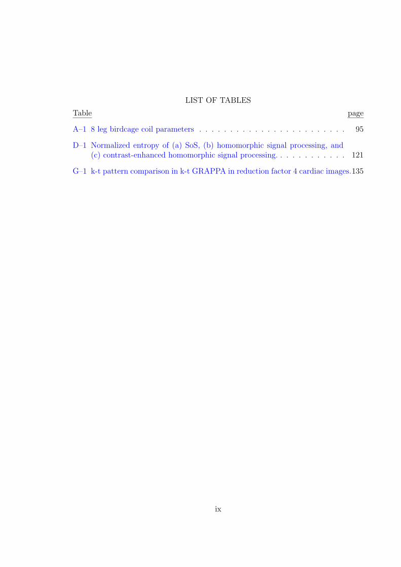
A–1 8 leg birdcage coil parameters . . . . . . . . . . . . . . . . . . . . . . . . 95

D–1 Normalized entropy of (a) SoS, (b) homomorphic signal processing, and(c) contrast-enhanced homomorphic signal processing. . . . . . . . . . . . 121

G–1 k-t pattern comparison in k-t GRAPPA in reduction factor 4 cardiac images.135

ix

LIST OF FIGURES

Figure page

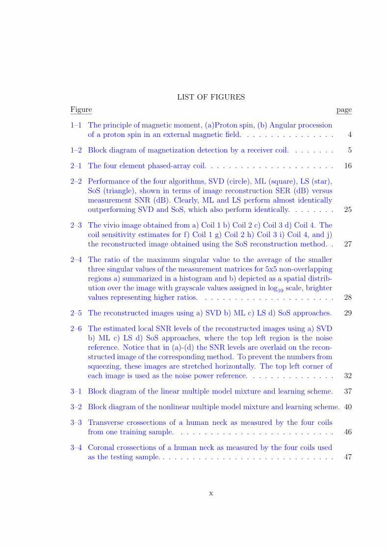
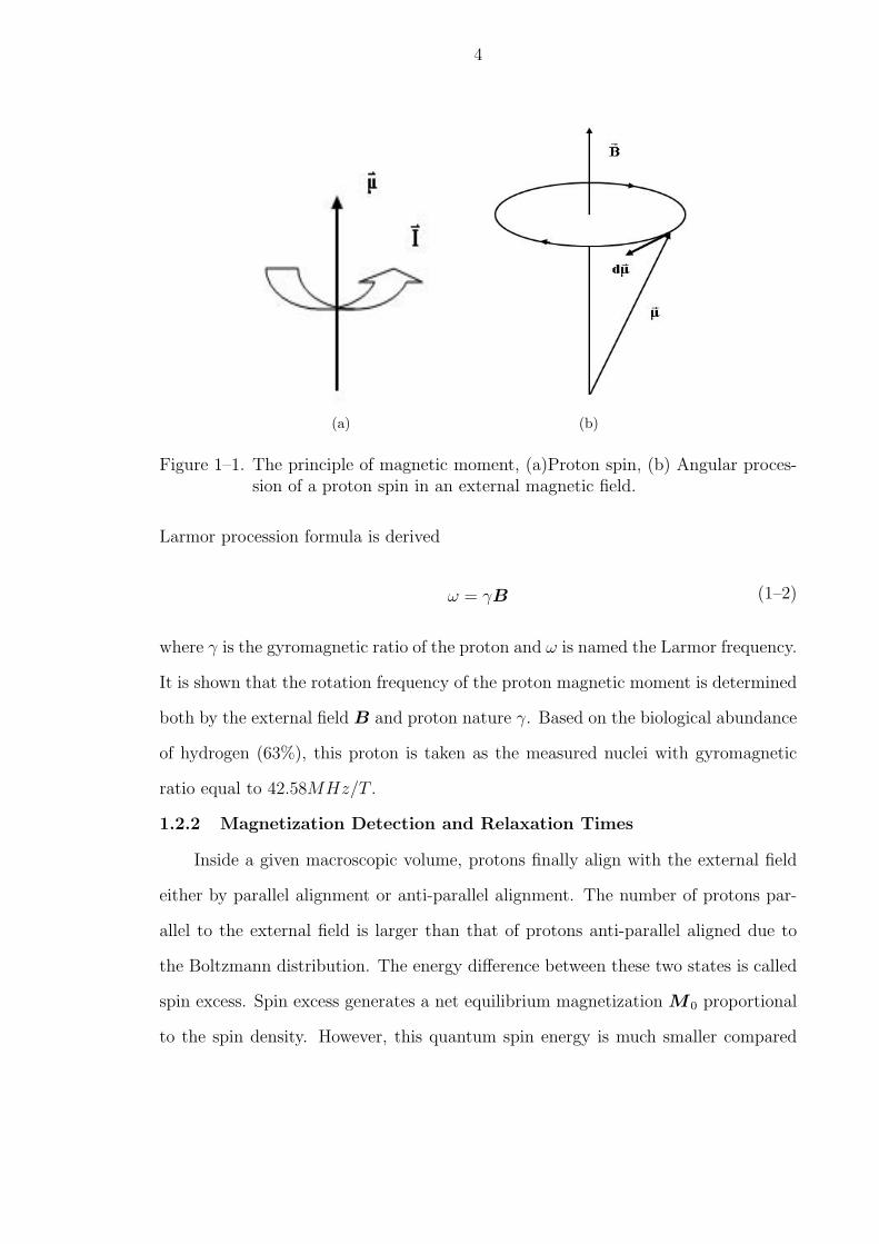
1–1 The principle of magnetic moment, (a)Proton spin, (b) Angular processionof a proton spin in an external magnetic field. . . . . . . . . . . . . . . . 4

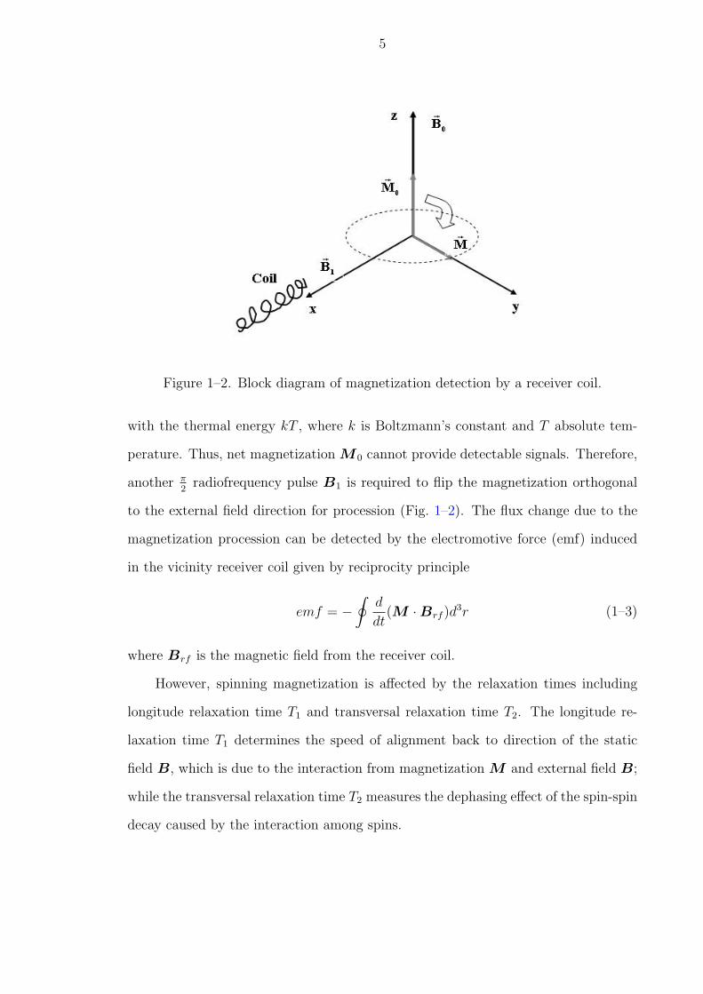
1–2 Block diagram of magnetization detection by a receiver coil. . . . . . . . 5

2–1 The four element phased-array coil. . . . . . . . . . . . . . . . . . . . . . 16

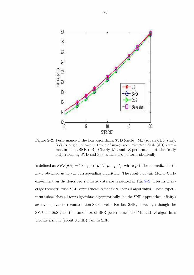
2–2 Performance of the four algorithms, SVD (circle), ML (square), LS (star),SoS (triangle), shown in terms of image reconstruction SER (dB) versusmeasurement SNR (dB). Clearly, ML and LS perform almost identicallyoutperforming SVD and SoS, which also perform identically. . . . . . . . 25

2–3 The vivio image obtained from a) Coil 1 b) Coil 2 c) Coil 3 d) Coil 4. Thecoil sensitivity estimates for f) Coil 1 g) Coil 2 h) Coil 3 i) Coil 4, and j)the reconstructed image obtained using the SoS reconstruction method. . 27

2–4 The ratio of the maximum singular value to the average of the smallerthree singular values of the measurement matrices for 5x5 non-overlappingregions a) summarized in a histogram and b) depicted as a spatial distrib-ution over the image with grayscale values assigned in log10 scale, brightervalues representing higher ratios. . . . . . . . . . . . . . . . . . . . . . . 28

2–5 The reconstructed images using a) SVD b) ML c) LS d) SoS approaches. 29

2–6 The estimated local SNR levels of the reconstructed images using a) SVDb) ML c) LS d) SoS approaches, where the top left region is the noisereference. Notice that in (a)-(d) the SNR levels are overlaid on the recon-structed image of the corresponding method. To prevent the numbers fromsqueezing, these images are stretched horizontally. The top left corner ofeach image is used as the noise power reference. . . . . . . . . . . . . . . 32

3–1 Block diagram of the linear multiple model mixture and learning scheme. 37

3–2 Block diagram of the nonlinear multiple model mixture and learning scheme. 40

3–3 Transverse crossections of a human neck as measured by the four coilsfrom one training sample. . . . . . . . . . . . . . . . . . . . . . . . . . . 46

3–4 Coronal crossections of a human neck as measured by the four coils usedas the testing sample. . . . . . . . . . . . . . . . . . . . . . . . . . . . . . 47

x

3–5 Desired reconstructed image, (a) estimated by averaging the SoS recon-struction for each coil image sample, (b) SNR performance of the estimateddesire. . . . . . . . . . . . . . . . . . . . . . . . . . . . . . . . . . . . . . 48

3–6 Adaptive learning performance, (a) Learning curve of winner models forthe model number 4,8,16, (b) Learning curve of the linear mixture ofcompetitive linear models system for the model number 4,8,16. . . . . . . 49

3–7 Learning curve of the nonlinear mixture of competitive linear models sys-tem for the model number 4. . . . . . . . . . . . . . . . . . . . . . . . . . 50

3–8 The reconstruction image, (a) From one transverse training sample bynonlinear mixture of local linear experts, (b) The SNR performance of thereconstruction. . . . . . . . . . . . . . . . . . . . . . . . . . . . . . . . . 50

3–9 Pixel classification for the model number 2, 4, 8, 16. . . . . . . . . . . . . 51

3–10 Reconstructed images and their SNR performances from the mixture ofcompetitive linear models system with the model number 16 and the coilnumber 4, 36. . . . . . . . . . . . . . . . . . . . . . . . . . . . . . . . . . 52

3–11 Reconstructed test images for a coronal crossection from a human neck,(a) SoS without whitening (b) SoS with whitening (c) Linear mixture ofmodels, (d) Nonlinear mixture of models. . . . . . . . . . . . . . . . . . . 53

3–12 SNR performances of the reconstructed test images for a coronal crossec-tion from a human neck, (a) SoS without whitening (b) SoS with whitening(c) Linear mixture of models, (d) Nonlinear mixture of models. . . . . . 54

3–13 Image quality measure, (a)-(b) The two reconstructions by nonlinear mix-tures of models using two near idential 4 coil samples, (c) The noise powerfrom the subtration of the two reconstruction images in (a). . . . . . . . 55

4–1 Block diagrom of the nonlinear multiple model mixture and learning scheme. 58

4–2 Histogram of output error from the well-trained MLP network by MSE. . 59

4–3 Adaptive learning performance, (a) The information potential learningcurve, (b) The kernel variance anealing curve. . . . . . . . . . . . . . . . 60

4–4 The reconstruction images of the coronal image by (a) ITL training and(b) MSE training. . . . . . . . . . . . . . . . . . . . . . . . . . . . . . . . 61

4–5 The SNR performance of the reconstruction images of the coronal imageby (a) ITL training and (b) MSE training. . . . . . . . . . . . . . . . . . 62

5–1 Block diagram of autoassociative network. . . . . . . . . . . . . . . . . . 69

5–2 The block diagram of competitive subspace projection methodology. . . . 71

xi

5–3 Three dimensional synthetic data, (a) projected to its first and seconddimension, where the third dimension is insignificant in classification (b)clustering data in (a) by k-means, (c) clustering data in (a) by optimallyintegrated adaptive learning (OIAL), (d) clustering data in (a) by com-petitive subspace projection (CSP). The intersected lines in (c) and (d)represent the two projection axes for each cluster. . . . . . . . . . . . . . 77

5–4 The learning curve in the second phase of training from competitive sub-space projection for M = 1, 2, 3 (The mean square error (MSE) is normal-ized by the input signal power). . . . . . . . . . . . . . . . . . . . . . . . 79

5–5 The projection axes for the number of the projection axes M = 2 andmodel number K = 3 after the second phase training of competitive sub-space projection is completed. . . . . . . . . . . . . . . . . . . . . . . . . 80

5–6 The cluster centroids for model number K = 4 and projection axes M = 2. 82

5–7 The cluster centroids for model number K = 3 and projection axes M = 2. 83

5–8 The four basis images (1-2 upper row and 3-4 lower row from left to right)are determined by NMF using real fMRI data. . . . . . . . . . . . . . . . 84

5–9 The encoding time series corresponds to four basis images by NMF usingreal fMRI data. . . . . . . . . . . . . . . . . . . . . . . . . . . . . . . . . 85

5–10 The temporal maxima plot for temporal clustering analysis (TCA) method. 86

5–11 Functional region localization by (a) temporal clustering analysis (b) non-negative matrix factorization and (c) competitive subspace projection. . . 87

A–1 Transmit only birdcage coil flow chart. . . . . . . . . . . . . . . . . . . . 96

A–2 Receiver coil flow chart, with C1, C2 are the parallel combination of a20pF capacitor and a 1-15pF adjustable capacitor; C3,C8 are the parallelcombination of a 4.7pF capacitor, a 91pF capacitor, and a 39pF capacitor;C4 is the parallel combination of a 3.9pF capacitor and a 1-15pF adjustablecapacitor; C5, C7 are the parallel combination of a 91pF capacitor and a39pF capacitor; C6 is the parallel combination of a 18pF capacitor and a1-15pF adjustable capacitor . . . . . . . . . . . . . . . . . . . . . . . . . 97

A–3 Schematic representation of a single transmit/receive switching circuit forprotection of the receiving preamplifier. . . . . . . . . . . . . . . . . . . . 98

A–4 Block diagram of the quadrature transmit coil, and receive- only phasedarray setup. . . . . . . . . . . . . . . . . . . . . . . . . . . . . . . . . . . 99

B–1 Synthetic data example. (a) Original noisy step function signal xn, (b)transformed (squared) signal yn, and (c) the true and the measured SNRlevels. . . . . . . . . . . . . . . . . . . . . . . . . . . . . . . . . . . . . . 107

xii

B–2 Reconstruction images and their SNR performance. (a) SoS, (b) SNR ofSoS. . . . . . . . . . . . . . . . . . . . . . . . . . . . . . . . . . . . . . . 109

B–3 Reconstruction images and their SNR performance. (a) logrithm of SoS,(b) SNR of logrithm of SoS. . . . . . . . . . . . . . . . . . . . . . . . . . 110

B–4 Reconstruction images and their SNR performance. (a) median filteredSoS, (b) SNR of median filtered SoS. . . . . . . . . . . . . . . . . . . . . 110

D–1 Canonic form for homomorphic signal processor. . . . . . . . . . . . . . . 115

D–2 Photograph of the phased array coil, transmit coil, and cabling. . . . . . 117

D–3 Vivo sagittal images of cat spinal cord from coil 1-4 and the spectralestimate of SoS. . . . . . . . . . . . . . . . . . . . . . . . . . . . . . . . . 118

D–4 (Upper row) Spatial distribution of the coil sensitivities for four coil sig-nals. (Lower row) Spectral distribution of the coil sensitivities for four coilsignals. . . . . . . . . . . . . . . . . . . . . . . . . . . . . . . . . . . . . . 119

D–5 The reconstruction image contrast versus the high-pass filter cutoff fre-quency and the stopband magnitude. . . . . . . . . . . . . . . . . . . . . 120

D–6 High-pass filter to eliminate coil sensitivities. . . . . . . . . . . . . . . . . 121

D–7 Reconstructed images. (a) Sum-of-squares (sos), (b) homomorphic signalprocessing, (c) contrast-enhanced homomorphic signal processing, and (d)reconstruction from the filtered coil sensitivities. . . . . . . . . . . . . . . 122

D–8 The pdf distribution of the reconstructed images. . . . . . . . . . . . . . 123

E–1 SoS of axial phantom data. . . . . . . . . . . . . . . . . . . . . . . . . . 126

E–2 High-pass and low-pass filter with order 4 and cutoff frequency at 64. . . 127

E–3 Central PE line from Reconstructions of homoSENSE of MSE = 0.23%,SENSE of MSE=2.19% compared with SoS. . . . . . . . . . . . . . . . . 128

F–1 Reconstruction of variable density imaging with 64 ACS lines and R = 4;(a) SENSE, MSE 1.96%; (b) Hybrid1dSENSE, MSE 1.71%; (c) SoS . . . 131

G–1 k-t trajectory in k-t GRAPPA. . . . . . . . . . . . . . . . . . . . . . . . 136

G–2 k-t pattern comparison in k-t GRAPPA in R = 5 cardiac images. . . . . 137

xiii

Abstract of Dissertation Presented to the Graduate Schoolof the University of Florida in Partial Fulfillment of theRequirements for the Degree of Doctor of Philosophy

COMPETITIVE MIXTURE OF LOCAL LINEAR EXPERTS FOR MAGNETICRESONANCE IMAGING

By

Rui Yan

May 2006

Chair: Jose C. PrincipeMajor Department: Electrical and Computer Engineering

Magnetic resonance imaging (MRI) is an important contemporary research field

propelled by expected clinical gains. MRI includes many interesting specialties. Re-

cently the data acquisition time in scanning patients became a critical issue. The

collection time of MRI images can be reduced at a cost of device complexity by using

multiple phased-array coils, which bring the problem of adequately combining multi-

ple coil images. In this dissertation, the problem of combining images obtained from

multiple MRI coils is investigated from a statistical signal processing point-of-view

with the goal of improving signal-to-noise-ratio (SNR) in the reconstructed images.

A new adaptive learning strategy using competitive learning as well as local linear ex-

perts is developed by treating the problem as function approximation. The proposed

method has the ability to train on a set of images and generalize its performance to

previously unseen images.

To validate the effectiveness of the adaptive method in MRI imaging, the com-

petitive mixture of experts was also tested in the extraction of information from

functional MRI (fMRI) images. The problem is to localize the functional pattern

xiv

corresponding to an external stimulus. Although this problem has been widely inves-

tigated using a block paradigm (i.e. processing synchronized with the external stimu-

lus), the proposed competitive mixtures model provides a self-organizing method that

can be especially useful in fMRI experiments when the response time is unknown.

To our knowledge, it is the first time that competitive learning is included into fMRI

signal analysis with good results.

xv

CHAPTER 1INTRODUCTION

1.1 Literature Review of Magnetic Resonance Imaging

Magnetic resonance imaging (MRI) is an imaging technique using radiofrequency

waves in a strong magnetic field mostly for inner human body examination. This

method can provide images with better quality than regular x-rays and CAT scans

for soft-tissues inside the body. Widely used as a noninvasive diagnostic tool in the

medical community, MRI is used to detect the early evidence of many ailments of

soft tissues such as brain abnormalities, coronary artery diseases and disorders of the

ligaments, etc.

1.1.1 History of MRI

The phenomenon of magnetic resonance imaging was independently discovered

by Bloch [1] and Purcell et al. [2] in 1946, which led to their Nobel Prize in 1952.

The relaxation times of tissues and tumors were found to be different by Dama-

dian in 1971 [3]. This discovery opened a promising application area for MRI. In

1973 Lauterbur [4] proposed magnetic resonance imaging using the back projection

method, for which he shared the Nobel prize in 2003. Ernst et al. [5] introduced the

Fourier Transform of the k-space sampling into 2D imaging, resulting in the modern

MRI technique and a shared Nobel prize in 1991.

1.1.2 fMRI

In the last decade, MRI imaging has been subdivided into two main categories.

One technique images time-varying processes within an image series and is called

functional MRI (fMRI) [6]. The purpose of this technique is to understand how func-

tional regions inside the brain respond to external stimuli. The information between

1

2

the functional regions of the brain and the cognitive operations has been investi-

gated [7]. The temporal partitioned activity demonstrates functional independence

with respect to the localized spatiality inside the brain [8]. The challenges remain

in localizing brain function when there is no priori knowledge available about a time

window in which a stimulus may elicit response. Thus there is no timing for the

brain’s response to align. The spatial active regions can still be located according to

the temporal response activated by a single stimulus [9]. Therefore fMRI provides a

method to understand the mapping between brain structures and their functions.

1.1.3 Image Reconstruction in Phased-Array MRI

Another research aspect focuses on fast imaging with multiple receiver coils.

The increased equipment complexity increases the signal-to-noise-ratio (SNR) by ap-

proximately combining the coil images from the different coils. Thus for a certain

SNR image quality level, phased-array imaging techniques can dramatically reduce

the scanning time, which has the benefits of reducing the motion artifacts of the

image. Roemer et al. proposed a pixel by pixel reconstruction method, named sum-

of-squares (SoS), to reconstruct coil images [10]. They showed that this method loses

only 10% of the maximum possible signal-to-noise-ratio (SNR) with no priori infor-

mation of the coils’ positions or RF field maps. This result sets the foundation of

phased-array image reconstruction and demonstrates its prevalence in the industry.

Based on SoS, a substantial body of research has focused on sophisticated techniques

for phase encoding together with the use of gradient coils. This work includes the sen-

sitivity encoding for fast MRI (SENSE) technique [11] and simultaneous acquisition

of spatial harmonics (SMASH) imaging [12]. Both methods reduce the scanning time

by undersampling along the gradient-echo direction from k-space in parallel data col-

lection. Debbins et al. [13] suggested adding the images coherently after their relative

phases were properly adjusted by another calibration scan. This method increased

the imaging rate by reducing demands, such as bandwidth and memory, while it kept

3

much of the SNR performance compared to SoS. Walsh et al. used adaptive filters to

improve SNR in the image [14]. Kellman and McVeigh proposed a method that can

use the degrees of freedom inherent to the phased array for ghost artifact cancellation

by a constrained SNR optimization [15]. This method also needs a priori informa-

tion on reference images without distortion to estimate coil sensitivities. Bydder et

al. proposed a reconstruction method that estimated the coil sensitivities from the

smoothened coil images to reduce noise effects [16]. A Bayesian method using itera-

tive maximum likelihood with a priori information in coil sensitivities was presented

recently by Yan et al. [17]. Recently image reconstruction methods incorporating lo-

cal coil sensitivity features have been proposed such as parallel imaging with localized

sensitivities (PILS) [18], local reconstruction [19], etc.

1.2 Magnetic Resonance Imaging Basics

1.2.1 Interaction of a Proton Spin with a Magnetic Field

Magnetic resonance imaging originates from understanding the nature of a proton

spin. It is the proton spin rather than the electron spin which is applicable in MRI

due to its field homogeneity as well as being noninvasive to the human body [20, 21].

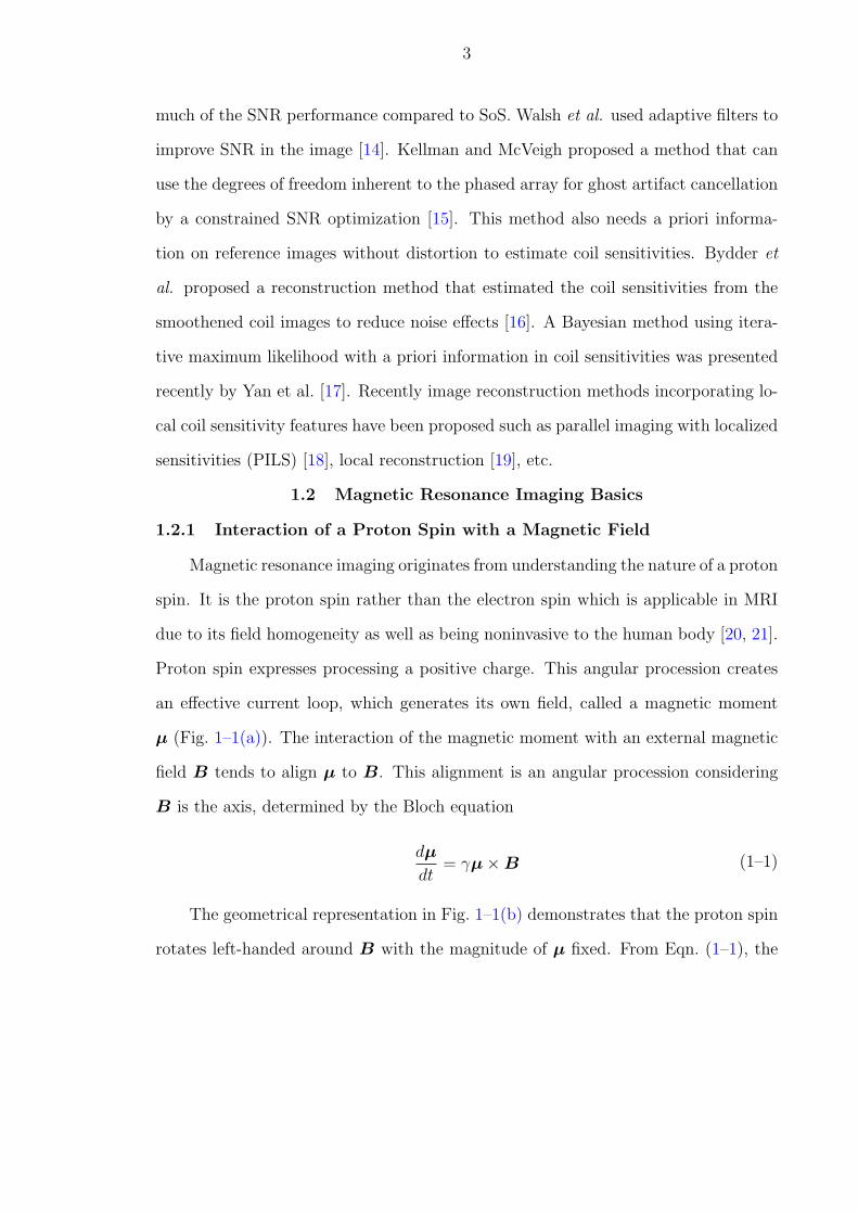
Proton spin expresses processing a positive charge. This angular procession creates

an effective current loop, which generates its own field, called a magnetic moment

µ (Fig. 1–1(a)). The interaction of the magnetic moment with an external magnetic

field B tends to align µ to B. This alignment is an angular procession considering

B is the axis, determined by the Bloch equation

dµ

dt= γµ×B (1–1)

The geometrical representation in Fig. 1–1(b) demonstrates that the proton spin

rotates left-handed around B with the magnitude of µ fixed. From Eqn. (1–1), the

4

(a) (b)

Figure 1–1. The principle of magnetic moment, (a)Proton spin, (b) Angular proces-sion of a proton spin in an external magnetic field.

Larmor procession formula is derived

ω = γB (1–2)

where γ is the gyromagnetic ratio of the proton and ω is named the Larmor frequency.

It is shown that the rotation frequency of the proton magnetic moment is determined

both by the external field B and proton nature γ. Based on the biological abundance

of hydrogen (63%), this proton is taken as the measured nuclei with gyromagnetic

ratio equal to 42.58MHz/T .

1.2.2 Magnetization Detection and Relaxation Times

Inside a given macroscopic volume, protons finally align with the external field

either by parallel alignment or anti-parallel alignment. The number of protons par-

allel to the external field is larger than that of protons anti-parallel aligned due to

the Boltzmann distribution. The energy difference between these two states is called

spin excess. Spin excess generates a net equilibrium magnetization M 0 proportional

to the spin density. However, this quantum spin energy is much smaller compared

5

Figure 1–2. Block diagram of magnetization detection by a receiver coil.

with the thermal energy kT , where k is Boltzmann’s constant and T absolute tem-

perature. Thus, net magnetization M 0 cannot provide detectable signals. Therefore,

another π2

radiofrequency pulse B1 is required to flip the magnetization orthogonal

to the external field direction for procession (Fig. 1–2). The flux change due to the

magnetization procession can be detected by the electromotive force (emf) induced

in the vicinity receiver coil given by reciprocity principle

emf = −∮

d

dt(M ·Brf )d

3r (1–3)

where Brf is the magnetic field from the receiver coil.

However, spinning magnetization is affected by the relaxation times including

longitude relaxation time T1 and transversal relaxation time T2. The longitude re-

laxation time T1 determines the speed of alignment back to direction of the static

field B, which is due to the interaction from magnetization M and external field B;

while the transversal relaxation time T2 measures the dephasing effect of the spin-spin

decay caused by the interaction among spins.

6

1.2.3 Magnetic Resonance Imaging

The key for imaging is to map the measured signals from the receiver coil with

the spatial locations. This can be achieved by applying a linearly spatial varying field

B +Gz, taking z direction as an example. So the received signal proportional to the

Larmor frequency ω(z) = γ(B + Gz) gives spatial slice information in z direction.

The relationship between the received signal and the spin density is given by the

Fourier Transform

x(k) =

∫ρ(z)e−i2πkzdz (1–4)

where ρ(z) is the one dimensional spin density and k(t) = γ2π

∫ t

0G(τ)dτ represents the

spatial frequency in k-space. The ρ(z) reflects image intensity and can be resolved

by an inverse Fourier Transform

ρ(z) =

∫x(k)ei2πkzdk (1–5)

Instead of the above 1D imaging, two dimensional spatial extension is easy to

accomplish by adding one more encoding direction. Suppose that phased-array coils

consisting of nc coils are used for the parallel data collection and let (xk, yk), k =

1, · · · , nc be the coordinate of the kth coil. Let x, y, z be orthogonal unit vectors

that span the Cartesian coordinate system under consideration, and suppose that a

suitable gradient magnetic field is applied to enable selective excitation of a thin slice

parallel to the (x,y) plane, say z = z0. At a given coordinate x, y, z0 and time t, let

Gx(t) and Gy(t) be the strength of the external magnetic field and define

kx(t) =

∫ t

0

Gx(τ)dτ

ky(t) =

∫ t

0

Gy(τ)dτ

(1–6)

7

Then, for a given kth receiver coil, the received time domain signal can be written as

xk(t) = e−iω0t

∫

x

∫

y

ρ(x, y)Ck(x, y)e−iλ(kx(t)(x−xk)+ky(t)(y−yk))dxdy + ek(t) (1–7)

where λ is a constant, and ρ(x, y) is proportional to the ”transverse magnetiza-

tion” (which is essentially the quantity of interest in the imaging), Ck(x, y) is the

sensitivity and ek(t) is noise both from the kth coil.

Equation (1–7) shows that the received signal x(t) is equal to the 2D Fourier

transform of the multiplication of the true pixel value ρ(x, y) and the coil sensitivity

Ck(x, y) sampled at kx(t) and ky(t).

After the inverse Fourier Transform is applied to the received k-space signal xk,

the resulting spatial signal sk(i, j) from coil k at coordinate (i, j) is the observed by

sk(i, j) = ρck(i, j) + nk(i, j), k = 1, 2, · · · , nc (1–8)

where nk(i, j) is complex-valued (Gaussian), wide sense stationary (WSS), zero-mean,

spatially white noise, which is possibly correlated across coils with covariance matrix

Q (spatiotemporally constant due to the WSS assumption [10, 22, 23]). Note that

the noise correlation, if properly compensated for, does not pose a limitation to the

achievable image quality [24]. In this signal model, the specific values of the coil

sensitivities are, in general, not known. However, some a priori knowledge in the

form of statistical distributions or structural constraints (such as spatial smoothness)

may be available.

1.3 Main contribution and introduction to appendix

The follow-up dissertation starts in chapter 2 with the optimal reconstruction

with known coil sensitivities. The maximum likelihood estimation gives the best

reconstruction with the known coil senstitivities. However, coil sensitivities is not

known a prior information in practice. The conventional sum-of-squares (SoS) method

solves the problem by estimating the coil sensitivities from pixel based data itself.

8

The dissertation demonstrates that SoS is an optimal linear combination base on

the signal-to-noise-ratio (SNR) analysis while the optimality is hard to satisfy in

practice. This disadvantage drives us to research novel reconstruction methods. By

incorporating the local smoothness property of coil sensitivities, three statistical im-

age reconstructions are proposed, named as singular value decomposition method,

Bayesian maximum-Likelihood reconstruction, and least squares with smoothness

penalty. These methods gains a 1-2dB SNR improvement compared with SoS. Al-

though the statistical methods give analytical solutions, they don’t have the capabil-

ity to manipulate historical data. Therefore, chapter 3 switches to adaptive learning

methods to extract features from historical scanning images. Once the adaptive net-

work is well trained, it can be generalized to other unknown scanning images. Com-

petitive learning combined with local linear experts is proposed in this dissertation

to implement the divide-and-conquer strategy in this function approximation case.

Such competitive learning topology incorporates intelligence into the adaptive net-

work to decouple the subtasks which has weak correlations in between. By training

a considerable amount of samples, the SNR improvement in the test image is signifi-

cant. Chapter 4 further this idea to information theoretical learning, where the error

criterion changes from mean square error to Renyi’s entropy. This is an extension

from second order statistics to higher order statistics. This competitive learning idea

is extended from supervised learning to unsupervised learning by proposing compet-

itive subspace projection in chapter 5. It is applied in functional MRI area and helps

to locate the activated spatial and temporal patterns inside brain. As a summary,

conclusions consisting of discussion and some proposed future work are described in

chapter 6.

Besides the main body of the dissertation, some complimentary work is worth

to mention. As we know, the MRI scanning with phased array coils specify different

coil configuration to different parts of patients or phantoms. Thus the coil design

9

needs careful consideration in a certain scanning case. Appendix A briefly describes

the four element birdcage coil used in the data collection.

Medical image quality is always a tough but interesting topic which measures the

amount of true object information extracted. The difficulty is due to lack of knowledge

of the true visual system, the noise and the blurring effect. Normally Signal-to-noise

ratio (SNR) measures the image noise while contrast-to-noise ratio (CNR) measures

the blurring effect. In case of pixel based image reconstruction, blurring effect is

ignorable and SNR is normally used as the image quality measure in full sampled

data case. However, nonlinear transformation changes the second order statistics.

Thus SNR measurement may give a fake image quality evaluation. Appendix B

describes the problem in detail. In order to conquer this problem, appendix C gives

a image quality speculation using nonparametric pdf estimation.

Except for the proposed statistical image reconstruction methods all in image

space, appendix D gives another perspective in modeling this problem in spectral

domain. Homomorphic signal processing helps bridges the filtering process between

spectral domain and the image domain. The final quantitative entropy in image

quality is also an interesting measurement.

The following three Appendix chapters describes my intern work in Invivo Cor-

poration. In partial parallel acquisition (PPA), it attracts much interest to sample the

k-space using variable density. Naquist sampling is usually at low frequency and un-

dersampling is usually at high frequency. Thus Naquist sampling conserves the image

energy and leads to high SNR in final reconstruction; the undersampling reduces the

scanning time by the acceleration factor. However, the combination from the recon-

structions of the two parts separately is a challenge. The ring effect is obvious in final

reconstruction if the two parts are naturally separately; on the other hand, filtering

the two parts may incorporate bias into the final reconstruction as well. Appendix

E gives an optimal filter design strategy to minimize the bias effect with smoothing

10

filter. Appendix F extends the k-space sampling to an arbitrary trajectory. Thus the

partial parallel image reconstruction is generalized by an inverse problem in hybrid

space. Dynamic imaging with undersampling is a hotspot. People are interested in

different reconstruction methods, such as k-t BLAST, k-t SENSE and k-t GRAPPA,

etc. Little work is done on how the k-t sampling trajectory affects the reconstruction

performance. Appendix G gives an optimal search criterion in finding the optimal

k-t trajectory related to k-t GRAPPA method.

CHAPTER 2STATISTICAL IMAGE RECONSTRUCTION METHODS

2.1 Optimal Reconstruction with Known Coil Sensitivities

It is well-known in the statistical signal processing literature that for complex-

valued received signals, assuming that the coil sensitivities are known, the SNR-

optimal linear combination of the measurements for estimating r(i, j) is given by

ρ(i, j) =cH(i, j)Q−1s(i, j)

cH(i, j)Q−1c(i, j)(2–1)

where H denotes the conjugate-transpose (Hermitian) operation, c(i, j) is the vector

of coil sensitivities and s(i, j) is the vector of measurements for pixel (i, j). The SNR-

optimality of this reconstruction method among all linear combiners can be proved,

for example, by applying the Cauchy-Schwartz inequality [25]. The SNR for this

reconstruction method can be determined to be |ρ|2||c||2/σ2, where σ2 is the noise

power (of both real and imaginary parts).

2.2 Sum-of-squares (SoS)

The sum-of-squares (SoS) method, proposed by Roemer et al. as a pixel by pixel

reconstruction method [10], is extensively implemented in the industry due to its high

image reconstruction quality and simple math calculation. This method estimates the

coil sensitivity ck at the kth coil as ck

ck = sk/

√√√√N∑

k=1

|sk|2 (2–2)

11

12

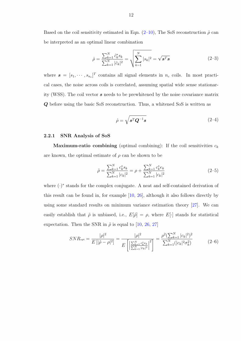
Based on the coil sensitivity estimated in Eqn. (2–10), The SoS reconstruction ρ can

be interpreted as an optimal linear combination

ρ =

∑Nk=1 c∗ksk∑Nk=1 |ck|2

=

√√√√N∑

k=1

|sk|2 =√

sT s (2–3)

where s = [s1, · · · , snc ]T contains all signal elements in nc coils. In most practi-

cal cases, the noise across coils is correlated, assuming spatial wide sense stationar-

ity (WSS). The coil vector s needs to be prewhitened by the noise covariance matrix

Q before using the basic SoS reconstruction. Thus, a whitened SoS is written as

ρ =

√sT Q−1s (2–4)

2.2.1 SNR Analysis of SoS

Maximum-ratio combining (optimal combining): If the coil sensitivities ck

are known, the optimal estimate of ρ can be shown to be

ρ =

∑Nk=1 c∗ksk∑Nk=1 |ck|2

= ρ +

∑Nk=1 c∗kek∑Nk=1 |ck|2

(2–5)

where (·)∗ stands for the complex conjugate. A neat and self-contained derivation of

this result can be found in, for example [10, 26], although it also follows directly by

using some standard results on minimum variance estimation theory [27]. We can

easily establish that ρ is unbiased, i.e., E[ρ] = ρ, where E[·] stands for statistical

expectation. Then the SNR in ρ is equal to [10, 26, 27]

SNRopt =|ρ|2

E [|ρ− ρ|2] =|ρ|2

E

[∣∣∣PN

k=1 c∗kekPNk=1 |ck|2

∣∣∣2] =

ρ2(∑N

k=1 |ck|2)2

∑Nk=1(|ck|2σ2

k)(2–6)

13

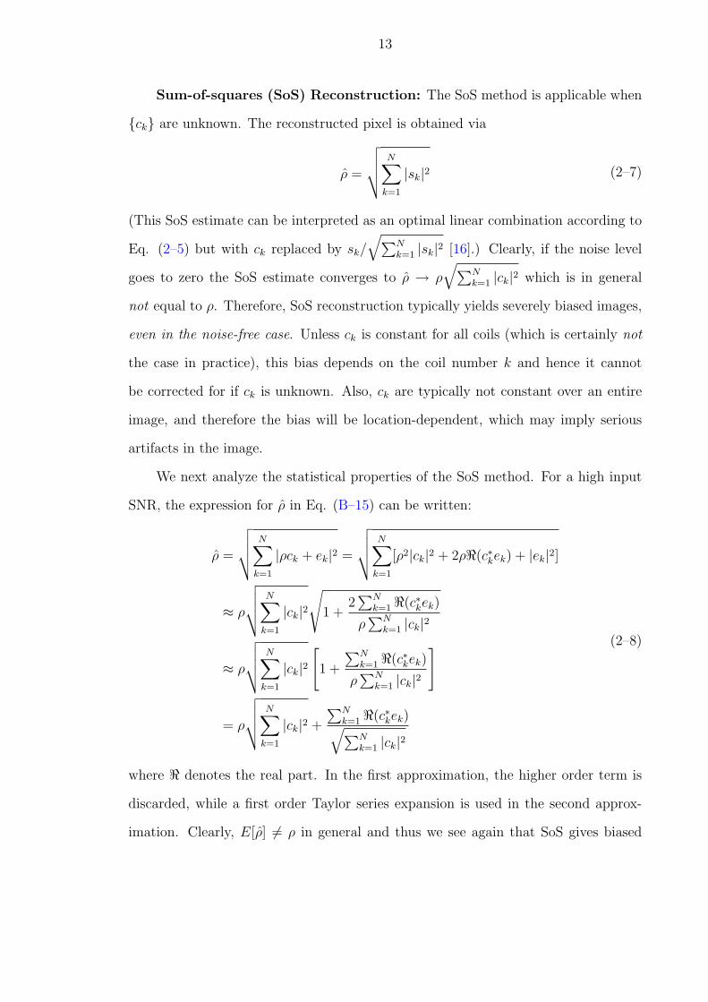
Sum-of-squares (SoS) Reconstruction: The SoS method is applicable when

ck are unknown. The reconstructed pixel is obtained via

ρ =

√√√√N∑

k=1

|sk|2 (2–7)

(This SoS estimate can be interpreted as an optimal linear combination according to

Eq. (2–5) but with ck replaced by sk/√∑N

k=1 |sk|2 [16].) Clearly, if the noise level

goes to zero the SoS estimate converges to ρ → ρ√∑N

k=1 |ck|2 which is in general

not equal to ρ. Therefore, SoS reconstruction typically yields severely biased images,

even in the noise-free case. Unless ck is constant for all coils (which is certainly not

the case in practice), this bias depends on the coil number k and hence it cannot

be corrected for if ck is unknown. Also, ck are typically not constant over an entire

image, and therefore the bias will be location-dependent, which may imply serious

artifacts in the image.

We next analyze the statistical properties of the SoS method. For a high input

SNR, the expression for ρ in Eq. (B–15) can be written:

ρ =

√√√√N∑

k=1

|ρck + ek|2 =

√√√√N∑

k=1

[ρ2|ck|2 + 2ρ<(c∗kek) + |ek|2]

≈ ρ

√√√√N∑

k=1

|ck|2√

1 +2∑N

k=1<(c∗kek)

ρ∑N

k=1 |ck|2

≈ ρ

√√√√N∑

k=1

|ck|2[1 +

∑Nk=1<(c∗kek)

ρ∑N

k=1 |ck|2

]

= ρ

√√√√N∑

k=1

|ck|2 +

∑Nk=1<(c∗kek)√∑N

k=1 |ck|2

(2–8)

where < denotes the real part. In the first approximation, the higher order term is

discarded, while a first order Taylor series expansion is used in the second approx-

imation. Clearly, E[ρ] 6= ρ in general and thus we see again that SoS gives biased

14

images. The SNR of ρ is obtained as:

SNRSoS =

(ρ√∑N

k=1 |ck|2)2

E

[∣∣∣∣PN

k=1 <(c∗kek)√PNk=1 |ck|2

∣∣∣∣2] =

ρ2(∑N

k=1 |ck|2)2

∑Nk=1(|ck|2σ2

k)(2–9)

which is equal to the same as the SNR for optimal combining with known coil sen-

sitivities (see Eq. (2–6)). Therefore, from a pure SNR point of view, SoS is optimal

for high input SNR.

2.2.2 Conclusion

SoS reconstruction method possesses many advantages. First, the SoS method

asymptotically approaches reconstruction optimality as all measurement (coil) signal-

to-noise-ratio (SNR) levels increase [28]. This high SNR performance ensures the final

reconstruction image quality, which is the most important virtue of SoS. Second, it

gives an unbiased estimate in the noise-free case. As we can see, if the noise level

goes to zero the SoS estimate converges to ρ → ρ√∑N

k=1 |ck|2. With ck estimated in

Eqn. (2–10),∑N

k=1 |ck|2 is one. Thus this SoS estimate ρ approaches the true pixel

value ρ, which also explains the reason why choosing such coil sensitivity estimator in

Eqn. (2–10). Besides, SoS doesn’t need any prior information. On one hand, with no

need for prescan or other information about the magnetic field, data collection is sim-

plified. On the other hand, no statistical assumption concerning the coil sensitivities

is predetermined and thus reduces the modeling error.

However, the widely-used sum-of-squares method has its own disadvantages.

Though it has the asymptotical SNR optimality property, the condition for this op-

timality, which is the high measurement SNR condition, is not always satisfied in

practice [28], especially in phased-arrays, where the coils measure only a portion of

the image. This creates the problem of considering pure noise pixels equally weighted

to pixels with actual signal. Another potential disadvantage for the SoS method

and other SoS based methods (e.g., SENSE & SMASH ) lies within the statistical

15

assumption of spatial wide sense stationarity (WSS) of the noise. Since, in general,

the noise covariance matrix Q is not known a priori, a region consisting of pure noise

pixels must be used to estimate it empirically. This often requires a manual selec-

tion of the noisy pixels or another reference scan containing only noise, under the

additional assumptions that the noise statistics are stationary within each imaging

trial and are independent from the object being imaged. If the noise exhibits local

properties in the spatial domain (e.g., the noise statistics differs from the signal region

to the background region), the noise covariance estimated from the global space or a

certain local space distorts or ignores some effective information and thus hurts the

reconstruction.

2.3 Reconstruction Methods Using Prior Information on CoilSensitivities

In this section, I present three image reconstruction methods for phased array

MRI that are optimal in the least-squares or maximum-likelihood sense. To this end,

one of the following two assumptions will be made:

A1. The coil sensitivities remain approximately constant over a small region Ω

consisting of N pixels, i.e., c(i, j) = cfor(i, j) ∈ Ω.

B1. The coil sensitivity profiles vary smoothly with the spatial location, within the

regions of interest.

In order to justify these assumptions, consider the images of a cat spinal cord shown

in Fig. D–3(a)-D–3(d) taken using the 4-coil phased array shown in Fig. 2–1 (4.7T,

TR=1000ms, TE=15ms, FOV=10 5cm, matrix=256128, slice thickness=2mm, sweep

width=26khz, 1 average). Regarding the SoS as a linear combination methodology,

the equivalent coil sensitivity estimates produced by this algorithm are found in

Eqn. (2–10). These estimated coil sensitivity profiles generated by the SoS are also

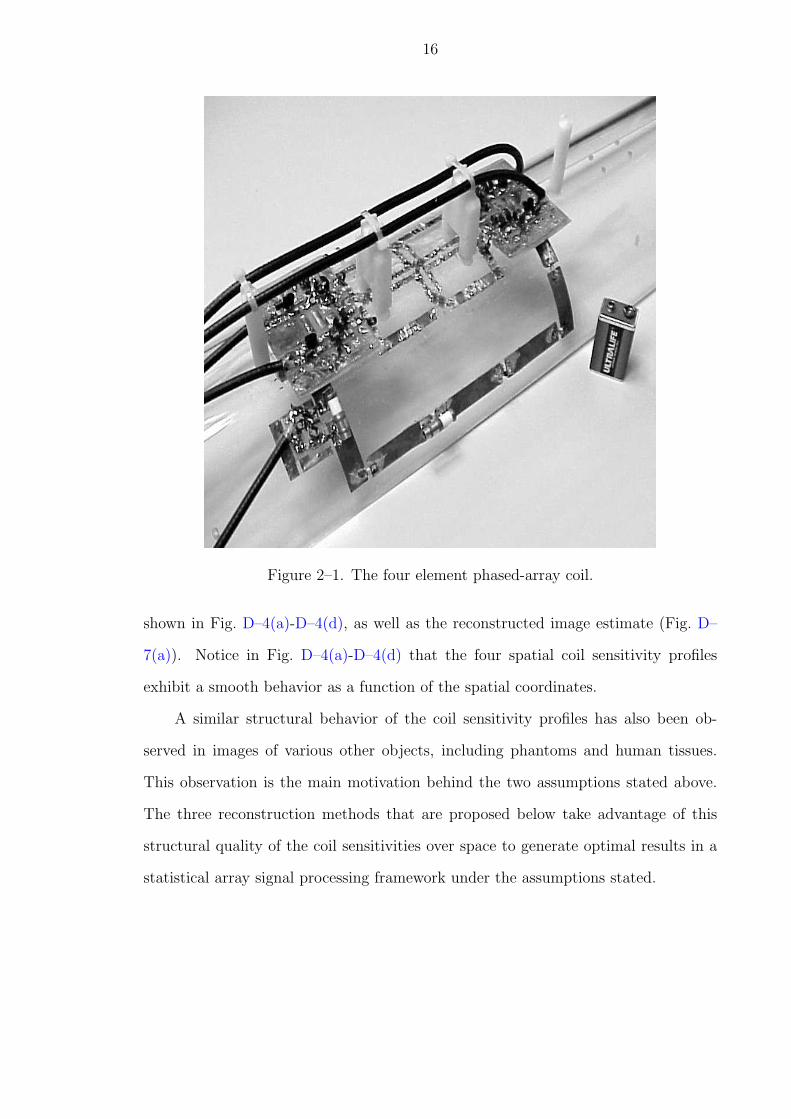
16

Figure 2–1. The four element phased-array coil.

shown in Fig. D–4(a)-D–4(d), as well as the reconstructed image estimate (Fig. D–

7(a)). Notice in Fig. D–4(a)-D–4(d) that the four spatial coil sensitivity profiles

exhibit a smooth behavior as a function of the spatial coordinates.

A similar structural behavior of the coil sensitivity profiles has also been ob-

served in images of various other objects, including phantoms and human tissues.

This observation is the main motivation behind the two assumptions stated above.

The three reconstruction methods that are proposed below take advantage of this

structural quality of the coil sensitivities over space to generate optimal results in a

statistical array signal processing framework under the assumptions stated.

17

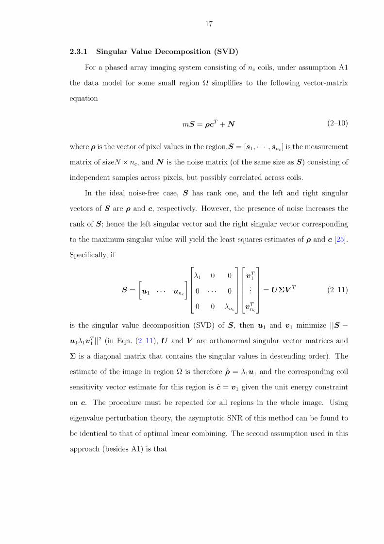
2.3.1 Singular Value Decomposition (SVD)

For a phased array imaging system consisting of nc coils, under assumption A1

the data model for some small region Ω simplifies to the following vector-matrix

equation

mS = ρcT + N (2–10)

where ρ is the vector of pixel values in the region,S = [s1, · · · , snc ] is the measurement

matrix of sizeN × nc, and N is the noise matrix (of the same size as S) consisting of

independent samples across pixels, but possibly correlated across coils.

In the ideal noise-free case, S has rank one, and the left and right singular

vectors of S are ρ and c, respectively. However, the presence of noise increases the

rank of S; hence the left singular vector and the right singular vector corresponding

to the maximum singular value will yield the least squares estimates of ρ and c [25].

Specifically, if

S =

[u1 · · · unc

]

λ1 0 0

0 · · · 0

0 0 λnc

vT1

...

vTnc

= UΣV T (2–11)

is the singular value decomposition (SVD) of S, then u1 and v1 minimize ||S −u1λ1v

T1 ||2 (in Eqn. (2–11), U and V are orthonormal singular vector matrices and

Σ is a diagonal matrix that contains the singular values in descending order). The

estimate of the image in region Ω is therefore ρ = λ1u1 and the corresponding coil

sensitivity vector estimate for this region is c = v1 given the unit energy constraint

on c. The procedure must be repeated for all regions in the whole image. Using

eigenvalue perturbation theory, the asymptotic SNR of this method can be found to

be identical to that of optimal linear combining. The second assumption used in this

approach (besides A1) is that

18

A3. The measurement matrix has an effective rank of one. Effectively, this is equiv-

alent to assuming that the coil measurement SNR levels are sufficiently high. In the

noise-free measurement case, A1 implies A3.

In order to demonstrate the validity of this assumption, we resort to the same cat

spinal cord image example shown in Fig. D–3. Fig. 2–4(a) shows the histogram of the

ratio between the largest singular value of the local measurement matrix to the mean

of the other three singular values (there are four singular values since there are four

coils). Since there are very few small singular value ratios, we conclude that in most

local regions the rank-one measurement matrix assumption accurately holds. In fact,

the noise-only regions dominantly contribute to the small singular-value-ratios. To

illustrate this fact, in Fig. 2–4(b) we also present the singular-value-ratio as a function

of spatial coordinate for the cat-spine image, using 5× 5 square local regions.

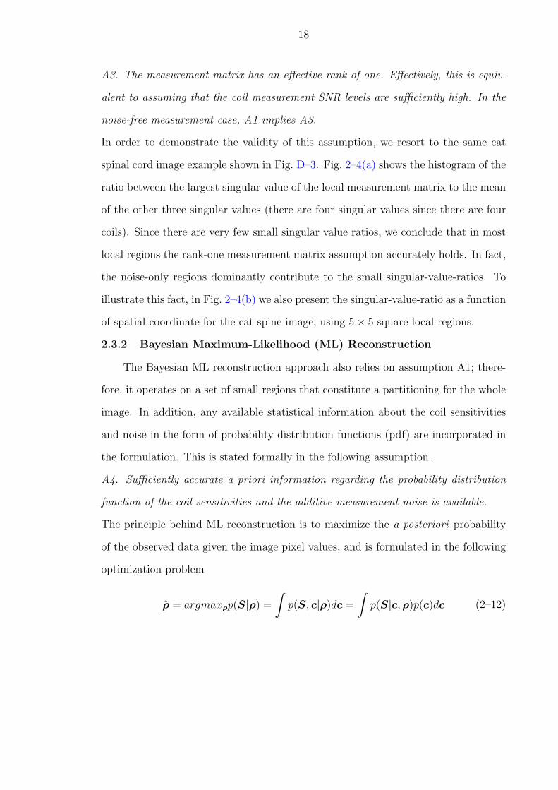
2.3.2 Bayesian Maximum-Likelihood (ML) Reconstruction

The Bayesian ML reconstruction approach also relies on assumption A1; there-

fore, it operates on a set of small regions that constitute a partitioning for the whole

image. In addition, any available statistical information about the coil sensitivities

and noise in the form of probability distribution functions (pdf) are incorporated in

the formulation. This is stated formally in the following assumption.

A4. Sufficiently accurate a priori information regarding the probability distribution

function of the coil sensitivities and the additive measurement noise is available.

The principle behind ML reconstruction is to maximize the a posteriori probability

of the observed data given the image pixel values, and is formulated in the following

optimization problem

ρ = argmaxρp(S|ρ) =

∫p(S, c|ρ)dc =

∫p(S|c, ρ)p(c)dc (2–12)

19

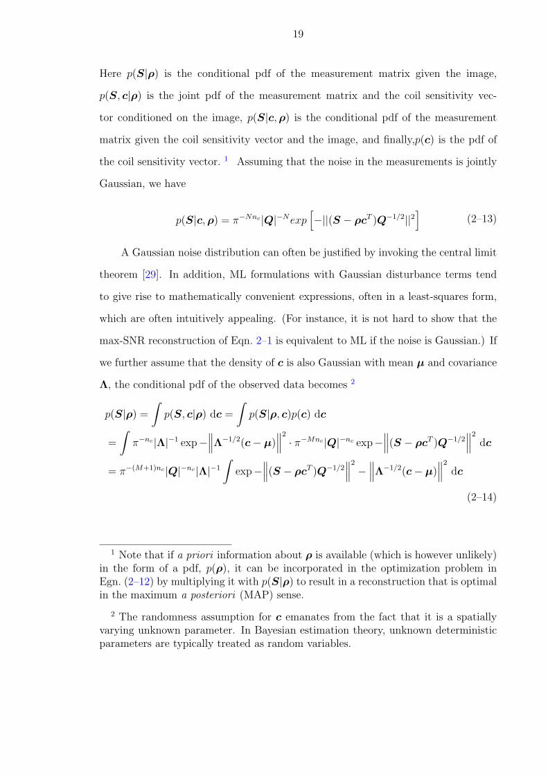
Here p(S|ρ) is the conditional pdf of the measurement matrix given the image,

p(S, c|ρ) is the joint pdf of the measurement matrix and the coil sensitivity vec-

tor conditioned on the image, p(S|c, ρ) is the conditional pdf of the measurement

matrix given the coil sensitivity vector and the image, and finally,p(c) is the pdf of

the coil sensitivity vector. 1 Assuming that the noise in the measurements is jointly

Gaussian, we have

p(S|c,ρ) = π−Nnc|Q|−Nexp[−||(S − ρcT )Q−1/2||2

](2–13)

A Gaussian noise distribution can often be justified by invoking the central limit

theorem [29]. In addition, ML formulations with Gaussian disturbance terms tend

to give rise to mathematically convenient expressions, often in a least-squares form,

which are often intuitively appealing. (For instance, it is not hard to show that the

max-SNR reconstruction of Eqn. 2–1 is equivalent to ML if the noise is Gaussian.) If

we further assume that the density of c is also Gaussian with mean µ and covariance

Λ, the conditional pdf of the observed data becomes 2

p(S|ρ) =

∫p(S, c|ρ) dc =

∫p(S|ρ, c)p(c) dc

=

∫π−nc|Λ|−1 exp−

∥∥∥Λ−1/2(c− µ)∥∥∥

2

· π−Mnc |Q|−nc exp−∥∥∥(S − ρcT )Q−1/2

∥∥∥2

dc

= π−(M+1)nc |Q|−nc |Λ|−1

∫exp−

∥∥∥(S − ρcT )Q−1/2∥∥∥

2

−∥∥∥Λ−1/2(c− µ)

∥∥∥2

dc

(2–14)

1 Note that if a priori information about ρ is available (which is however unlikely)in the form of a pdf, p(ρ), it can be incorporated in the optimization problem inEgn. (2–12) by multiplying it with p(S|ρ) to result in a reconstruction that is optimalin the maximum a posteriori (MAP) sense.

2 The randomness assumption for c emanates from the fact that it is a spatiallyvarying unknown parameter. In Bayesian estimation theory, unknown deterministicparameters are typically treated as random variables.

20

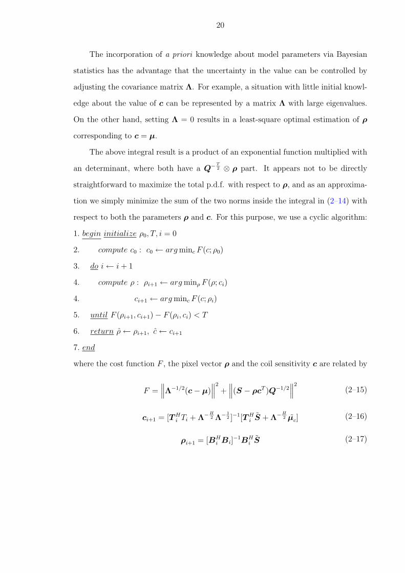
The incorporation of a priori knowledge about model parameters via Bayesian

statistics has the advantage that the uncertainty in the value can be controlled by

adjusting the covariance matrix Λ. For example, a situation with little initial knowl-

edge about the value of c can be represented by a matrix Λ with large eigenvalues.

On the other hand, setting Λ = 0 results in a least-square optimal estimation of ρ

corresponding to c = µ.

The above integral result is a product of an exponential function multiplied with

an determinant, where both have a Q−T2 ⊗ ρ part. It appears not to be directly

straightforward to maximize the total p.d.f. with respect to ρ, and as an approxima-

tion we simply minimize the sum of the two norms inside the integral in (2–14) with

respect to both the parameters ρ and c. For this purpose, we use a cyclic algorithm:

1. begin initialize ρ0, T, i = 0

2. compute c0 : c0 ← arg minc F (c; ρ0)

3. do i ← i + 1

4. compute ρ : ρi+1 ← arg minρ F (ρ; ci)

4. ci+1 ← arg minc F (c; ρi)

5. until F (ρi+1, ci+1)− F (ρi, ci) < T

6. return ρ ← ρi+1, c ← ci+1

7. end

where the cost function F , the pixel vector ρ and the coil sensitivity c are related by

F =∥∥∥Λ−1/2(c− µ)

∥∥∥2

+∥∥∥(S − ρcT )Q−1/2

∥∥∥2

(2–15)

ci+1 = [T Hi Ti + Λ−H

2 Λ− 12 ]−1[T H

i S + Λ−H2 µc] (2–16)

ρi+1 = [BHi Bi]

−1BHi S (2–17)

21

where ⊗ stands for the Kronecker product and

Bi = (Q−T2 ci)⊗ I, S = (Q−T

2 ⊗ I)

s1

...

snc

T i = (Q−T2 )⊗ ρi, µc = Λ− 1

2 µc

(2–18)

In an MRI application, we may obtain ρ and c either via analytical modeling

of the electromagnetic fields associated with the coils, or via calibration scans of a

phantom with known contrasts; by modulating the parameter Λ, we can directly

influence the accuracy of the prior knowledge of c. Such efforts to compute the

coil sensitivity patterns must use the finite-difference time-domain (FDTD) method,

which is a computational method to solve Maxwells equations. FDTD divides the

problem space into rectangular cells, called Yee-cells, and uses discrete time-steps [30,

31]. This approach has been successfully employed to compute the sensitivity patterns

of transmit and receive coils for MRI [32]. The noise covariance, on the other hand,

can be estimated from the coil images using portions of the frame that do not have

any signal.

Since a closed-form expression for the solution of this reconstruction algorithm

is not available, it is difficult to obtain an asymptotic SNR expression. Nevertheless,

since the solution is the fixed-point of the iterations, perturbation methods could be

used to obtain an SNR expression, possibly after tedious calculations.

2.3.3 Least Squares (LS) with Smoothness Penalty

Given the measurement model in Eqn. (1–8) and assumption A2, a simple and

intuitive approach is to solve a penalized least-squares (LS) problem to reconstruct

the image from the coil measurements. Recall that LS methods coincide with ML if

the error is Gaussian. A natural smoothness penalty function is one that attempts

to minimize the first and second order spatial derivatives of the coil sensitivities.

22

However, such an approach alone does not solve the problem, because the optimal

solution of a penalized LS criterion tends to yield images with large intensity. This is

so because decreasing the amplitude of the coil sensitivity profile decreases its deriv-

atives as well, causing the reconstructed image to be scaled up by the same amount.

Therefore, it appears necessary to also impose a penalty on the total energy of the

image. The resulting penalized least squares criterion, which has to be minimized to

obtain the optimal reconstructed image, is given in Eqn. (2–19)

J(ρ, c1, . . . , cnc) =(1− λ1 − λ2 − λ3)J0(ρ, c1, . . . , cnc) + λ1J1(c1, . . . , cnc)

+ λ2J2(c1, . . . , cnc) + λ3J3(ρ)

J0(ρ, c1, . . . , cnc) =nc∑

k=1

M∑i=1

N∑j=1

[sk(i, j)− ρ(i, j)ck(i, j)]2 + [sk(i, j)− ρ(i, j)ck(i, j)]

2

J1(c1, . . . , cnc) =nc∑

k=1

M∑i=2

N∑j=1

[ck(i− 1, j)− ck(i, j)]2 +

nc∑

k=1

M∑i=1

N∑j=2

[ck(i, j)− ck(i, j − 1)]2

=nc∑

k=1

(||A1ck||2 + ||A2cTk ||2

)

J2(c1, . . . , cnc) =nc∑

k=1

M∑i=3

N∑j=1

[ck(i, j)− 2ck(i− 1, j) + ck(i− 2, j)]2

+nc∑

k=1

M∑i=1

N∑j=3

[ck(i, j)− 2ck(i, j − 1) + ck(i, j − 2)]2

=nc∑

k=1

(||B1ck||2 + ||B2cTk ||2)

J3(ρ) =M∑i=1

N∑j=1

[ρ(i, j)]2 = ||ρ||2

(2–19)

where ρ now denotes the vector of pixel values for the whole image; hence no parti-

tioning is required here. Note that the penalty term in this LS formulation can be

23

interpreted as a Bayesian prior. 3 The gradient G of the cost function in (2–19) with

respect to the optimization variables W = [ρT , cT1 , . . . , cT

nc]T is

G =

∂J∂ρ

∂J∂c1

...

∂J∂cnc

= (1− λ1 − λ2 − λ3)G0 + λ1G1 + λ2G2 + λ3G3

G0 =

∂J0

∂ρ

∂J0

∂c1

...

∂J0

∂cnc

=

2∑nc

k=1[ρ¯ ck ¯ ck]

[c1 ¯ ρ¯ ρ− s1 ¯ ρ]

...

[cnc ¯ ρ¯ ρ− snc ¯ ρ]

G1 =

∂J1

∂ρ

∂J1

∂c1

...

∂J1

∂cnc

G2 =

∂J2

∂ρ

∂J2

∂c1

...

∂J2

∂cnc

=

0

2(BT1 B1c1 + c1B

T2 B2)

...

2(BT1 B1cnc + cncB

T2 B2)

G3 =

∂J3

∂ρ

∂J3

∂c1

...

∂J3

∂cnc

(2–20)

where¯ denotes element-wise vector product. In (2–20), Ai and Bi are non-symmetric

sparse Toeplitz matrices that arise from the matrix formulation of the first and second

order differences. In particular, A1 and A2 are (M-1)xM and (N-1)xN matrices with

1s on the main diagonal and -1s in the first upper diagonal, and B1 and B2 are

(M-2)xM and (N-2)xN matrices with 1s on the main diagonal, -2s in the first upper

diagonal, and 1s in the second upper diagonal. All other entries of these matrices

are zeros. Similar to the case of the Bayesian reconstruction algorithm, obtaining

an asymptotic SNR expression for this algorithm should be possible although it is

algebraically complicated.

3 More details on the relation between smoothness constraints and a priori infor-mation via Bayesian statistics can be found in [32].

24

In general, least squares criteria can be shown to be equivalent to the maximum

likelihood principle if the probability distributions under consideration are Gaussian,

or perhaps other symmetric unimodal functions where the peak of the distribution

corresponds to its mean value as well [27]. Besides the three statistical reconstruc-

tions, a image reconstruction method based on spectral decomposition is worth to

mention in Appendix D.

2.4 Results and Discussion

The performances of the proposed algorithms are first evaluated using synthetic

data. The data model for this data is as follows. A random image consisting of 9

pixels whose jth pixel value is drawn from Uniform [j, j + 1] and then normalized

such that the norm of the intensity vector is unity, ρT ρ = 1. The measurement

vector in each coil is obtained by sk = (rho + σek)ck, where c = [c1, · · · , c4]T is the

coil sensitivity vector (with each entry selected from Uniform [0, 1]), ek is zero-mean,

unit-covariance Gaussian noise (also independent across coils), and σ is the standard

deviation of the additive noise determined by the specific measurement SNR that is

being simulated. 4 All four algorithms (SVD, ML, LS, and SoS) are applied to this

synthetic data in 20000 Monte Carlo simulations for each measurement SNR level,

where all parameters are randomized as described above in every trial.

The image intensity estimate vectors of all four algorithms are normalized to

unity such that in the comparison with the ground truth (which is available in this

setup) using signal-to-error ratio (SER) without considering scaling errors. The SER

4 Note that this is not a very realistic situation, since in an actual MRI, the mea-surement SNR in a coil is also determined by its sensitivity coefficient. In this ex-ample, however, the noise is added to the image before coil sensitivity scaling isapplied, merely for convenience in representing results (such that a single SNR valuedescribes the data quality). In fact, it will become evident in the application to realdata that statistical signal processing approaches benefit more from this variabilityin measurement SNR of coils.

25

Figure 2–2. Performance of the four algorithms, SVD (circle), ML (square), LS (star),SoS (triangle), shown in terms of image reconstruction SER (dB) versusmeasurement SNR (dB). Clearly, ML and LS perform almost identicallyoutperforming SVD and SoS, which also perform identically.

is defined as SER(dB) = 10 log1 0 (||ρ||2/||ρ− ρ||2), where ρ is the normalized esti-

mate obtained using the corresponding algorithm. The results of this Monte-Carlo

experiment on the described synthetic data are presented in Fig. 2–2 in terms of av-

erage reconstruction SER versus measurement SNR for all algorithms. These experi-

ments show that all four algorithms asymptotically (as the SNR approaches infinity)

achieve equivalent reconstruction SER levels. For low SNR, however, although the

SVD and SoS yield the same level of SER performance, the ML and LS algorithms

provide a slight (about 0.6 dB) gain in SER.

26

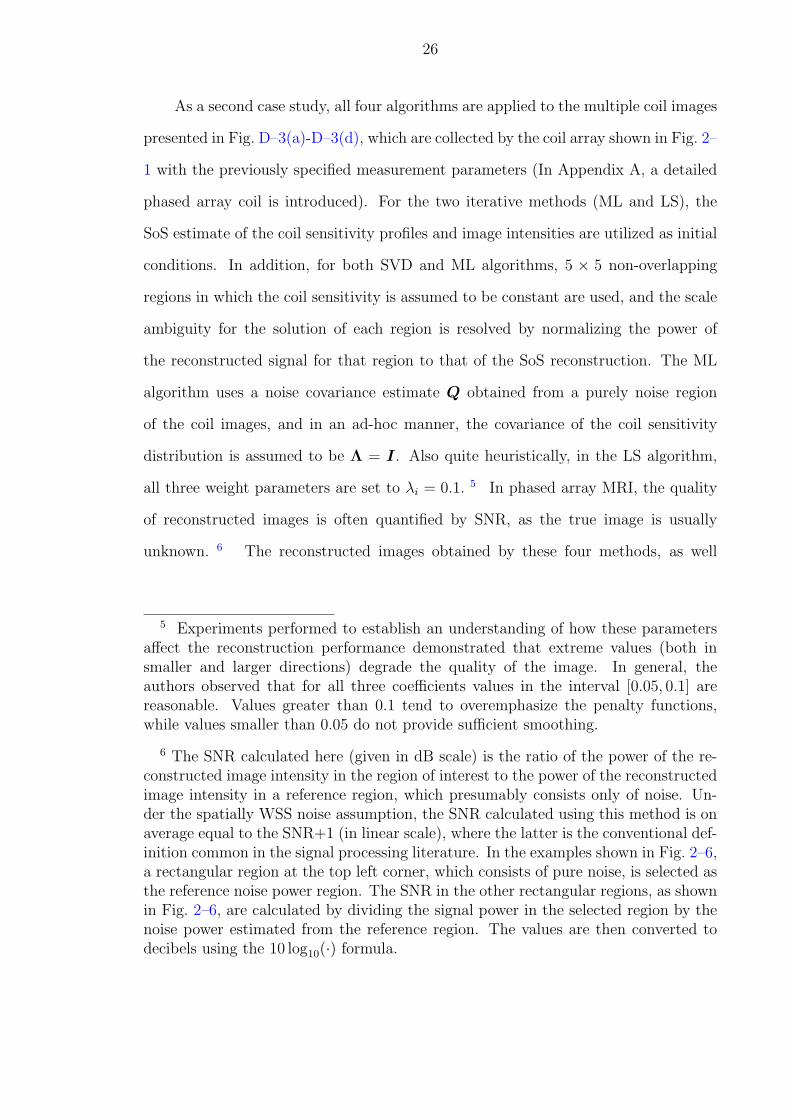
As a second case study, all four algorithms are applied to the multiple coil images

presented in Fig. D–3(a)-D–3(d), which are collected by the coil array shown in Fig. 2–

1 with the previously specified measurement parameters (In Appendix A, a detailed

phased array coil is introduced). For the two iterative methods (ML and LS), the

SoS estimate of the coil sensitivity profiles and image intensities are utilized as initial

conditions. In addition, for both SVD and ML algorithms, 5 × 5 non-overlapping

regions in which the coil sensitivity is assumed to be constant are used, and the scale

ambiguity for the solution of each region is resolved by normalizing the power of

the reconstructed signal for that region to that of the SoS reconstruction. The ML

algorithm uses a noise covariance estimate Q obtained from a purely noise region

of the coil images, and in an ad-hoc manner, the covariance of the coil sensitivity

distribution is assumed to be Λ = I. Also quite heuristically, in the LS algorithm,

all three weight parameters are set to λi = 0.1. 5 In phased array MRI, the quality

of reconstructed images is often quantified by SNR, as the true image is usually

unknown. 6 The reconstructed images obtained by these four methods, as well

5 Experiments performed to establish an understanding of how these parametersaffect the reconstruction performance demonstrated that extreme values (both insmaller and larger directions) degrade the quality of the image. In general, theauthors observed that for all three coefficients values in the interval [0.05, 0.1] arereasonable. Values greater than 0.1 tend to overemphasize the penalty functions,while values smaller than 0.05 do not provide sufficient smoothing.

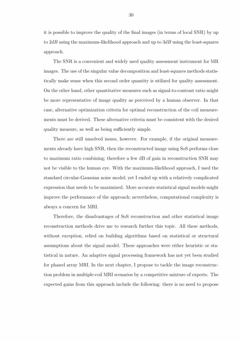
6 The SNR calculated here (given in dB scale) is the ratio of the power of the re-constructed image intensity in the region of interest to the power of the reconstructedimage intensity in a reference region, which presumably consists only of noise. Un-der the spatially WSS noise assumption, the SNR calculated using this method is onaverage equal to the SNR+1 (in linear scale), where the latter is the conventional def-inition common in the signal processing literature. In the examples shown in Fig. 2–6,a rectangular region at the top left corner, which consists of pure noise, is selected asthe reference noise power region. The SNR in the other rectangular regions, as shownin Fig. 2–6, are calculated by dividing the signal power in the selected region by thenoise power estimated from the reference region. The values are then converted todecibels using the 10 log10(·) formula.

27

(a) (b) (c) (d) (e)

(f) (g) (h) (i)

Figure 2–3. The vivio image obtained from a) Coil 1 b) Coil 2 c) Coil 3 d) Coil 4. Thecoil sensitivity estimates for f) Coil 1 g) Coil 2 h) Coil 3 i) Coil 4, and j)the reconstructed image obtained using the SoS reconstruction method.

as the estimated local SNR levels of these reconstructed images are presented in

Fig. 2–5& 2–6. By comparing the SNR estimates in Fig. 2–6(a)-2–6(d), we observe

that the SVD and SoS methods, in general, produce images with equal SNR levels

(although SVD is observed to be more sensitive to noise and measurement artifacts as

discussed below), whereas the ML approach improves the SNR by up to 2dB and the

LS approach improves the SNR by up to 3dB over the performance of SoS. However,

the correlation between SNR and image quality will be explained in Appendix B and

C.

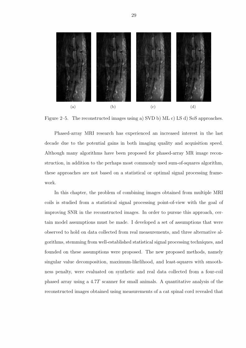
At first look, a clear artifact in the SVD reconstructed image shown in Fig. 2–

5(a) is visible. Although this artifact is not as visible in the other three reconstructed

28

0 20 40 60 80 1000

50

100

150

200

250

(a)

0

10

20

30

40

50

60

70

80

90

(b)

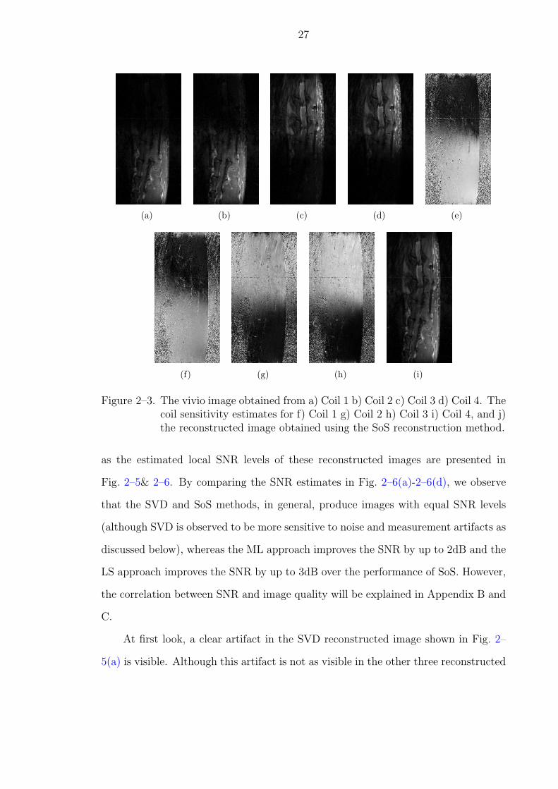
Figure 2–4. The ratio of the maximum singular value to the average of thesmaller three singular values of the measurement matrices for 5x5 non-overlapping regions a) summarized in a histogram and b) depicted as aspatial distribution over the image with grayscale values assigned in log10

scale, brighter values representing higher ratios.

images (Fig. 2–5(b)-D–7(a)) due to the small size of the figures, upon closer exami-

nation, we see that this horizontal artifact also exists in these images. The reason for

this artifact is identified as a horizontal measurement artifact that exists in all four

coil measurements at that location (most strongly seen in the first coil). This artifact,

along with measurement noise, is amplified in the SVD reconstruction method to the

highly visible level in Fig. 2–6(a). The reason for this amplification of noise and

outliers can be understood by investigating Fig. 2–4(b). The ratios of the maximum

singular values to minimum ones are not as large in the top half of the coil measure-

ment image as the same ratios in the bottom half of the image. Consequently, A3

is not as strongly satisfied in the top half as the bottom half. This causes the SVD

algorithm to pass the existing measurement noise to the reconstructed image with

some amplification. The artifact in the measurements is also amplified in the process.

29

(a) (b) (c) (d)

Figure 2–5. The reconstructed images using a) SVD b) ML c) LS d) SoS approaches.

Phased-array MRI research has experienced an increased interest in the last

decade due to the potential gains in both imaging quality and acquisition speed.

Although many algorithms have been proposed for phased-array MR image recon-

struction, in addition to the perhaps most commonly used sum-of-squares algorithm,

these approaches are not based on a statistical or optimal signal processing frame-

work.

In this chapter, the problem of combining images obtained from multiple MRI

coils is studied from a statistical signal processing point-of-view with the goal of

improving SNR in the reconstructed images. In order to pursue this approach, cer-

tain model assumptions must be made. I developed a set of assumptions that were

observed to hold on data collected from real measurements, and three alternative al-

gorithms, stemming from well-established statistical signal processing techniques, and

founded on these assumptions were proposed. The new proposed methods, namely

singular value decomposition, maximum-likelihood, and least-squares with smooth-

ness penalty, were evaluated on synthetic and real data collected from a four-coil

phased array using a 4.7T scanner for small animals. A quantitative analysis of the

reconstructed images obtained using measurements of a cat spinal cord revealed that

30

it is possible to improve the quality of the final images (in terms of local SNR) by up

to 2dB using the maximum-likelihood approach and up to 3dB using the least-squares

approach.

The SNR is a convenient and widely used quality assessment instrument for MR

images. The use of the singular value decomposition and least-squares methods statis-

tically make sense when this second order quantity is utilized for quality assessment.

On the other hand, other quantitative measures such as signal-to-contrast ratio might

be more representative of image quality as perceived by a human observer. In that

case, alternative optimization criteria for optimal reconstruction of the coil measure-

ments must be derived. These alternative criteria must be consistent with the desired

quality measure, as well as being sufficiently simple.

There are still unsolved issues, however. For example, if the original measure-

ments already have high SNR, then the reconstructed image using SoS performs close

to maximum ratio combining; therefore a few dB of gain in reconstruction SNR may

not be visible to the human eye. With the maximum-likelihood approach, I used the

standard circular-Gaussian noise model; yet I ended up with a relatively complicated

expression that needs to be maximized. More accurate statistical signal models might

improve the performance of the approach; nevertheless, computational complexity is

always a concern for MRI.

Therefore, the disadvantages of SoS reconstruction and other statistical image

reconstruction methods drive me to research further this topic. All these methods,

without exception, relied on building algorithms based on statistical or structural

assumptions about the signal model. These approaches were either heuristic or sta-

tistical in nature. An adaptive signal processing framework has not yet been studied

for phased array MRI. In the next chapter, I propose to tackle the image reconstruc-

tion problem in multiple-coil MRI scenarios by a competitive mixture of experts. The

expected gains from this approach include the following: there is no need to propose

31

or discover signal models that describe the measurements well (a must in statistical

signal processing approaches) and the local structure of the input space is naturally

extracted from the data. Thus the key difficulty to estimate the coil sensitivities is

avoided. Moreover, adaptive systems are more flexible and robust to inconsisten-

cies and nonstationarities in the data as they can be updated on-line while in use.

With a meaningful adaptation paradigm adaptive systems are able to approximate

optimal statistical signal processing approaches (to the limits set by the topology)

while requiring less design effort. However, the adaptive framework requires a desired

response for adaptation operation, as will be discussed below.

32

6dB 13dB 15dB 19dB 21dB 5.2dB

11dB 16dB 21dB 23dB 27dB 16dB







8.8dB 17dB 20dB 23dB 28dB 20dB




(a)

7.3dB 14dB 16dB 20dB 22dB 6.4dB












(b)

8.3dB 15dB 17dB 21dB 23dB 7.5dB












(c)

8.3dB 15dB 17dB 21dB 23dB 7.4dB13dB 18dB 24dB 25dB 29dB 18dB13dB 19dB 21dB 24dB 30dB 21dB15dB 22dB 23dB 26dB 29dB 21dB15dB 20dB 21dB 24dB 28dB 23dB18dB 22dB 21dB 23dB 28dB 22dB16dB 17dB 20dB 22dB 27dB 21dB14dB 18dB 23dB 25dB 29dB 22dB11dB 19dB 22dB 25dB 31dB 22dB11dB 21dB 24dB 28dB 31dB 23dB6.9dB 15dB 23dB 30dB 33dB 21dB5.1dB 17dB 24dB 28dB 32dB 16dB

(d)

Figure 2–6. The estimated local SNR levels of the reconstructed images using a)SVD b) ML c) LS d) SoS approaches, where the top left region is thenoise reference. Notice that in (a)-(d) the SNR levels are overlaid onthe reconstructed image of the corresponding method. To prevent thenumbers from squeezing, these images are stretched horizontally. Thetop left corner of each image is used as the noise power reference.

CHAPTER 3SUPERVISED LEARNING IN ADAPTIVE IMAGE RECONSTRUCTION

METHODS, PART A: MIXTURE OF LOCAL LINEAR EXPERTS

3.1 Local Patterns in Coil Profile

As we reviewed, fast MRI imaging using a phased-array of multiple coils has to

cope with an implicit inhomogeneous reception profile in each coil [33]. This feature is

described by coil sensitivity profiles, and explains the B1 field map generated from the

coil geometry. Due to the spatial configuration of phased-array coils, the sensitivities

of the coils are restricted to a finite region of space. This local coil sensitivity feature

is used in recent MRI image reconstruction such as parallel imaging with localized

sensitivities (PILS) [18], local reconstruction [19], etc.

Besides the sensitivity map locality, it is of interest whether the thermal noise

generated in the receiver coils possesses local property. The thermal noise Vnoise in

the coils is excited by the imaged lossy body in the coil vicinity, where the rms voltage

of the noise is given by Nyquist’s formula [34, 35]

Vnoise =√

4kTB∆fRL (3–1)

where k is the Boltzmann’s constant, TB the temperature of the body, ∆f the band-

width of the preamplifier attached to the coil and RL the equivalent loss resistance

of the coil. For a given designed coil system, the thermal noise Vnoise should solely

depend on RL. The loss resistance RL is affected by many factors, i.e., the geome-

tries of the coil and body, their positions relative to each other, the conductivity and

complex permittivity of the dielectric and the coil coupling. The load affects RL by

transferring the uncoupled coils into coupled and finally influence the generated noise.

This effect produces the local noise property distinct in the desired image region and

33

34

background image region. However, due to complex local structure inside the image

region, the noise property is hard to estimate there. Based on these local patterns

in coil profiles, an adaptive signal processing strategy is proposed to extract local

features and incorporate them into image reconstruction.

3.2 Competitive Learning

Competitive learning algorithms are widely used in pattern classification [36],

vector quantization [37], and time series prediction [38], etc. They employ competi-

tion among the processing elements (PEs) by lateral connection or a certain training

rule. The simple competitive learning with the winner-take-all (WTA) activation rule

leads to a PE underutilization [39]. Two other schemes, named as frequency-sensitive

competitive learning (FSCL) and the self-organizing map (SOM), are addressed to

solve this problem. FSCL incorporates the conscience term into the training to drive

all the PEs inside the network into competition [40]. The SOM method proposed by

Kohonen uses a soft competition scheme to adapt not only the activation PE but also

its neighborhood [41]. Competitive learning has also been used in image processing as

image compression [42], image segmentation [43] and color image quantization [44].

3.3 Multiple Local Models

The idea of using multiple simple and local models to represent complicated non-

linear systems has gained interest in recent years. The multiple model idea comes

from the following reasoning: if any nonlinear mapping or space representation can be

subdivided into different subset, the utilization of multiple models reduces the cou-

pling of different subsets and gives a better representation and mapping performance.

If each model is identically linear, this multiple model method is usually called local

linear model or local linear expert. In most cases, the parameter for learning multiple

models is based on competitive learning while the competition strategy is either com-

petitive or cooperative. However, it was stated that the cooperative and competitive

35

mixtures of local linear models in classification generalize better performance than

radial basis function (RBF) and MLP with a comparable number of parameters [45].

Function approximation is an interesting area to use local models in representing

a nonlinear input-output mapping. The idea of local linear modeling was applied in

predicting chaotic time series, where the nonlinear dynamics is learned by the local

approximation [46, 47], as well as in the nonlinear autoregressive model parameter

estimation given a Markov structure [48]. Jacobs et al. proposed a mixture of experts

network followed by a gated network, used in multispeaker vowel recognition [49].

This divide-and-conquer strategy first provides a new view of either modular version

of multilayer supervised network or an associative version of competitive learning.

The authors control the coupling among the multiple models by using a negative

log probability cost function. However, the gating weights are input-based and not

adapted to optimality. Fancourt introduced a cooperative fashion to the mixture of

experts network, where both the model parameters and gating weights are trained

by the Expectation-Maximization (EM) algorithm [50]. This method determines the

proportion of the datum which belongs to a single linear model according to its

posterior probability and combines the linear wiener solution in each model. The soft

competition actually provides a new data set strictly following the assumed Gaussian

distribution for each model, it may incorporate the modeling error into the final

estimation.

Another example in modular networks is applied to the local training of the

radial basis function (RBF). It shows that the k-nearest neighbor method (KNN) or

RBF network can be generalized to a local learning model based on different kernel

selection [51]. A local model networks which incorporates local learning to a radial

basis function (RBF) is proposed also in the divide-and-conquer strategy [52]. A

Growing Multi-Experts method is proposed as a novel modular network which adds

a local linear model to the RBF at the gating network stage [53]. In spite of the

36

network topology, it deploys a redundant experts removal algorithm to remove the

redundant models in order to exploit the optimal network architecture. Among these

methods, the parameter choices of the kernel (usually Gaussian kernel) needs careful

consideration. Based on the smooth tails of the Gaussian kernel, the decomposition

of the input space is somewhat overlapped, which means that the local properties

are not fully satisfied. Besides, the kernel parameter is adapted by the pure input

mapping, which doesn’t take the input-output mapping into account. Now I propose

to implement the competitive mixture of local linear experts method into image

reconstruction in phased-array MRI. It achieves simple local properties for each model

while the training is based on the input-output mapping while the gated network has

the universe approximation ability.

3.4 The Linear Mixture of Local Linear Experts for Phased-Array MRIReconstruction

In order to circumvent the difficulties associated with SoS, and to improve the

quality of the reconstructed image in terms of SNR, an adaptive training approach

with a mixture of experts can be employed [50]. In the case of MRI, it is possible

to obtain a sequence of training images from a phantom statistically representative

of the actual objects to be imaged, or equivalently, a training set of images from a

subject in the beginning of the session. The supervised adaptive training process

learns these sample properties and stores them in system weights. Once the image

reconstruction system is trained (calibrated) with this set of images, it can then be

utilized for reconstructing images from scans of other subjects (e.g., tissues). The

desired high quality output is formed by utilizing a standard image reconstruction

algorithm (such as SoS) on multiple scans of the training image set and averaging

the reconstructed images to generate a high SNR desired output image with di,j as

the desired output for pixel (i, j). An alternative to multiple images is to increase

the scan time to improve the quality of a single scan image. In training, the network

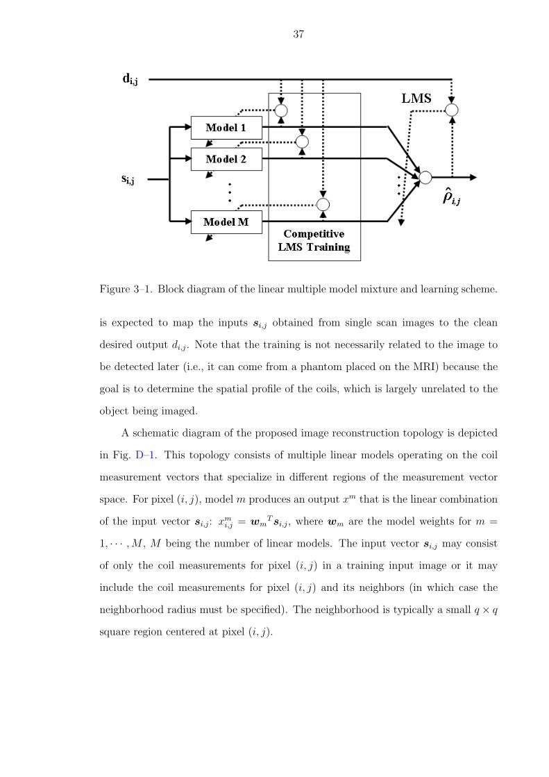
37

Figure 3–1. Block diagram of the linear multiple model mixture and learning scheme.

is expected to map the inputs si,j obtained from single scan images to the clean

desired output di,j. Note that the training is not necessarily related to the image to

be detected later (i.e., it can come from a phantom placed on the MRI) because the

goal is to determine the spatial profile of the coils, which is largely unrelated to the

object being imaged.

A schematic diagram of the proposed image reconstruction topology is depicted

in Fig. D–1. This topology consists of multiple linear models operating on the coil

measurement vectors that specialize in different regions of the measurement vector

space. For pixel (i, j), model m produces an output xm that is the linear combination

of the input vector si,j: xmi,j = wm

T si,j, where wm are the model weights for m =

1, · · · ,M , M being the number of linear models. The input vector si,j may consist

of only the coil measurements for pixel (i, j) in a training input image or it may

include the coil measurements for pixel (i, j) and its neighbors (in which case the

neighborhood radius must be specified). The neighborhood is typically a small q × q

square region centered at pixel (i, j).

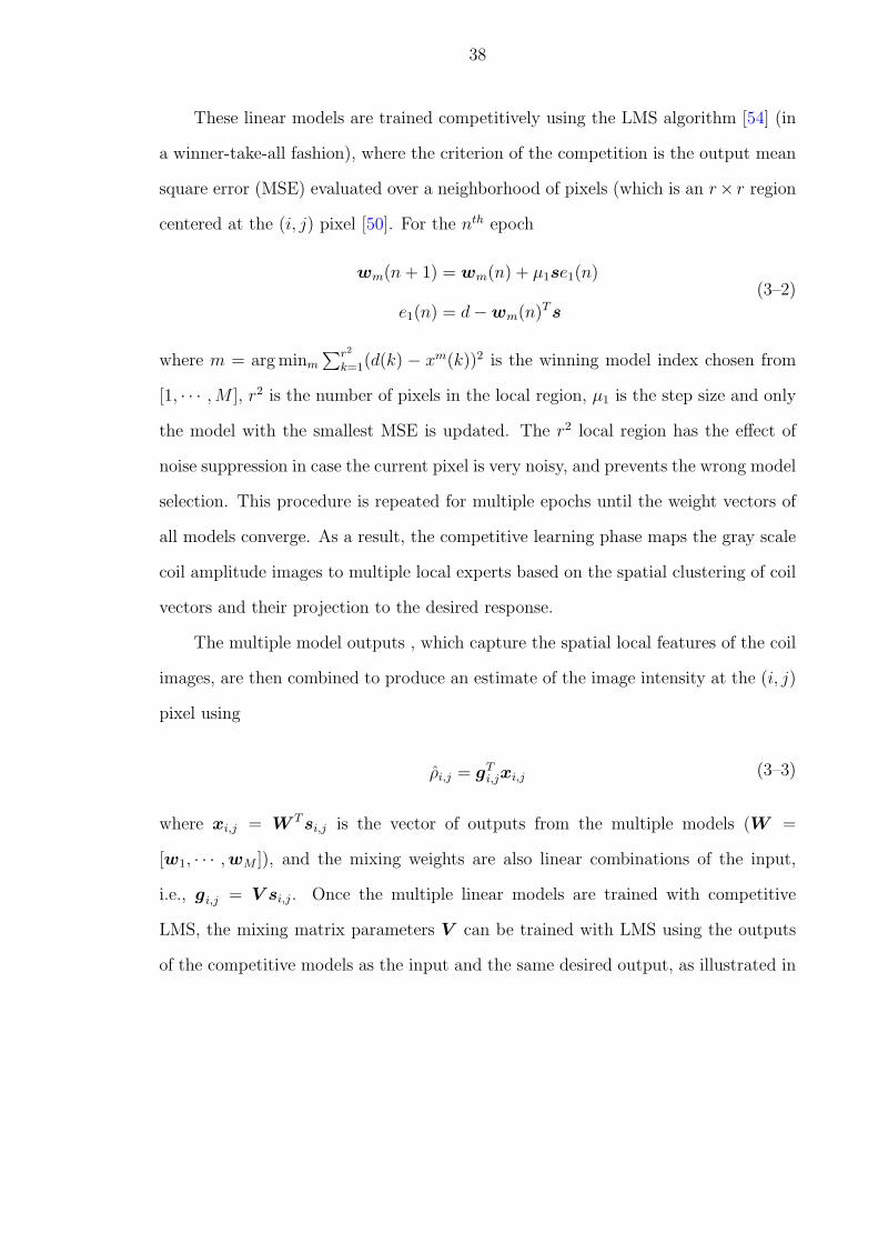
38

These linear models are trained competitively using the LMS algorithm [54] (in

a winner-take-all fashion), where the criterion of the competition is the output mean

square error (MSE) evaluated over a neighborhood of pixels (which is an r× r region

centered at the (i, j) pixel [50]. For the nth epoch

wm(n + 1) = wm(n) + µ1se1(n)

e1(n) = d−wm(n)T s

(3–2)

where m = arg minm

∑r2

k=1(d(k) − xm(k))2 is the winning model index chosen from

[1, · · · ,M ], r2 is the number of pixels in the local region, µ1 is the step size and only

the model with the smallest MSE is updated. The r2 local region has the effect of

noise suppression in case the current pixel is very noisy, and prevents the wrong model

selection. This procedure is repeated for multiple epochs until the weight vectors of

all models converge. As a result, the competitive learning phase maps the gray scale

coil amplitude images to multiple local experts based on the spatial clustering of coil

vectors and their projection to the desired response.

The multiple model outputs , which capture the spatial local features of the coil

images, are then combined to produce an estimate of the image intensity at the (i, j)

pixel using

ρi,j = gTi,jxi,j (3–3)

where xi,j = W T si,j is the vector of outputs from the multiple models (W =

[w1, · · · ,wM ]), and the mixing weights are also linear combinations of the input,

i.e., gi,j = V si,j. Once the multiple linear models are trained with competitive

LMS, the mixing matrix parameters V can be trained with LMS using the outputs

of the competitive models as the input and the same desired output, as illustrated in

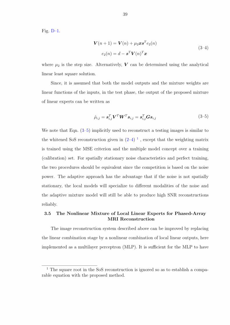
39

Fig. D–1.

V (n + 1) = V (n) + µ2xsT e2(n)

e2(n) = d− sT V (n)T x

(3–4)

where µ2 is the step size. Alternatively, V can be determined using the analytical

linear least square solution.

Since, it is assumed that both the model outputs and the mixture weights are

linear functions of the inputs, in the test phase, the output of the proposed mixture

of linear experts can be written as

ρi,j = sTi,jV

T W T si,j = sTi,jGsi,j (3–5)

We note that Eqn. (3–5) implicitly used to reconstruct a testing images is similar to

the whitened SoS reconstruction given in (2–4) 1 , except that the weighting matrix

is trained using the MSE criterion and the multiple model concept over a training

(calibration) set. For spatially stationary noise characteristics and perfect training,

the two procedures should be equivalent since the competition is based on the noise

power. The adaptive approach has the advantage that if the noise is not spatially

stationary, the local models will specialize to different modalities of the noise and

the adaptive mixture model will still be able to produce high SNR reconstructions

reliably.

3.5 The Nonlinear Mixture of Local Linear Experts for Phased-ArrayMRI Reconstruction

The image reconstruction system described above can be improved by replacing

the linear combination stage by a nonlinear combination of local linear outputs, here

implemented as a multilayer perceptron (MLP). It is sufficient for the MLP to have

1 The square root in the SoS reconstruction is ignored so as to establish a compa-rable equation with the proposed method.

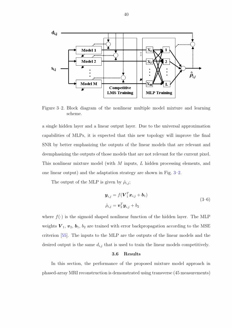
40

Figure 3–2. Block diagram of the nonlinear multiple model mixture and learningscheme.

a single hidden layer and a linear output layer. Due to the universal approximation

capabilities of MLPs, it is expected that this new topology will improve the final

SNR by better emphasizing the outputs of the linear models that are relevant and

deemphasizing the outputs of those models that are not relevant for the current pixel.

This nonlinear mixture model (with M inputs, L hidden processing elements, and

one linear output) and the adaptation strategy are shown in Fig. 3–2.

The output of the MLP is given by ρi,j;

yi,j = f(V T1 xi,j + b1)

ρi,j = vT2 yi,j + b2

(3–6)

where f(·) is the sigmoid shaped nonlinear function of the hidden layer. The MLP

weights V 1, v2, b1, b2 are trained with error backpropagation according to the MSE

criterion [55]. The inputs to the MLP are the outputs of the linear models and the

desired output is the same di,j that is used to train the linear models competitively.

3.6 Results

In this section, the performance of the proposed mixture model approach in

phased-array MRI reconstruction is demonstrated using transverse (45 measurements)

41

and coronal (9 measurements) fast collection human neck images in a 4-coil MRI sys-

tem (fast spin echo(FSE), TE=15ms, TR=150ms, ETL = 2, FOV = 40cm, slice

thickness = 5mm, matrix = 160×128, NEX=1). Sample images from the four coils

for both cross-sections are shown in Fig. 3–3 & 3–4, which is noisy due to the short

scanning time for each sample. All transverse cross-section measurements are used

for training and one of the coronal cross-section measurements (the one that is shown

in Fig. 3–4) is used for testing the resulting network. The desired reconstructed

image is estimated by averaging the SoS reconstruction for each training coil im-

age sample (Fig. 3–5(a)). Its high SNR performance demonstrates a clean and low

noise desired response (Fig. 3–5(b)). Both training and testing data sets consist of

magnitude images normalized to [−1, 1] before processing.

The training procedure, made in two stages, needs some special discussion. In

the first stage, the weights in the local linear experts are trained competitively by

LMS. The number of competitive models is selected to be M = 4 (as will be explained

below). The input vector si,j corresponds to only one pixel (i, j). The training of

the local models stops after 20 epochs with the step size µ1 = 0.01 demonstrated in

Fig. 3–6(a). After the weights in the first stage are well trained, the multiple expert

outputs are taken as the input to the second combination stage and di,j used in the

first stage is again taken as the desired response. The linear mixture finishes training

in 5 epochs with µ2 = 0.01 by LMS algorithm shown in Fig. 3–6(b). Alternatively,

the nonlinear mixture network is a 3-layer MLP network with one linear output PE,

5 hidden PEs and M input PEs corresponding to M multiple experts. The training

stops in 30 epochs with the step size µ2 = 0.005 by the backpropagation algorithm

shown in Fig. 3–7. The reconstructed image calculated from one training sample of

the transverse cross-sections by the trained nonlinear mixture of local linear experts

shows a peak SNR of 33 dB (Fig. 3–8), which is still 12 dB lower than the peak SNR

42

of the desired response image (Fig. 3–5). This SNR gap means that there is still room

for improvement in future research.

The coil measurements of the test image (coronal cross-section) are combined

using SoS (without and with whitening) as well as the proposed mixture model net-

work. Since a reference (a ground truth) is not available in MRI, typically the image

quality is measured by the empirical SNR measure, which in fact does not conform to

the traditional definition of SNR in signal processing. The procedure for computing

the SNR is as follows:

1. Find a reference region in the reconstructed image where there is no signal (i.e., a

pure noise region).

2. Compute the variance of the noise in this reference region.

3. For all other regions, compute the signal power (which includes both the actual

signal and the remaining noise in that region).

4. Calculate SNR in a region as the ratio of the power of the signal in that region

to the variance of the noise in the reference region. Convert SNR to dB. In order

to optimally configure the proposed method, parameter analysis is addressed now.

First, I demonstrate the specialization of the local linear models of the first stage dur-

ing training. The important question concerning the number of local linear models

is also addressed. Fig. 3–9 shows the spatial distribution of the pixels for a sample

image using trained multiple local models for the cases where M = 2, 4, 8, 16. One

can observe that the 2-model system basically segments the image into noise and

signal regions. As M is increased, the additional models help segment the signal and

noise regions to smaller partitions depending on their local statistics. As expected,

as the number of models is increased, the MSE of the winning models in training

converges to progressively lower value as shown in Fig. 3–6(a). However, the overall

MSE of the final output (after the combination of the multiple model outputs) does

not decrease significantly when the number of local linear models is increased above

43

M = 4(shown in Fig. 3–6(b)). Due to additional computational load and generaliza-

tion considerations, one should in practice select the smallest number of models that

yield satisfactory performance. In measuring the performance, the modeling MSE

and the SNR of the reconstructed image can be monitored simultaneously to make

a decision. In our MRI system, for example, M = 4 is a logical choice, and will be

used in the rest of the experiments.

Next, I study the effect of increasing the spatial filter order q (the neighborhood)

for each coil image in reconstructing the center pixel value. In general, the input

vector si,j for reconstructing pixel (i, j) can consist of all pixels in a neighborhood of

pixel (i, j) from all coils. For example, if a 3 × 3 region centered around pixel (i, j)

is selected, then the competing linear combiners become 9-tap 2-dimensional spatial

FIR filters on each coil, yielding a total of p = 4× 3× 3 = 36 input values, assuming

nc = 4 coils. This extension of the input vector to include neighboring pixels in the

reconstruction of the center pixel allows designing competing minimum-MSE spatial

filters for each coil. Increasing the size of these spatial filters will introduce additional

smoothing capabilities that help increase SNR. As an illustration, the performance

of the linear mixture of local linear experts approach is demonstrated on the coronal

cross-section reconstruction using noisy measurements from 4 coils. Compared to

the SNR performance of the competitive linear experts using only the center pixel (4-

dimensional input vector) shown in Fig. 3–10(a)&3–10(c), the SNR obtained by using

a 36-dimensional input (i.e., a 3×3 neighborhood for the FIR filters) shown in Fig. 3–

10(b)&3–10(d) is up to 4dB higher in the signal regions. This noise suppression is

achieved at the cost of some blurring of the sharp details in the reconstructed image,

due to the low-pass filtering effect of the increased-length spatial filters;so smaller

masks or multiple input multiple output combination method are advisable.

Now I analyze the advantage of nonlinear combination of experts. Since both the

linear and nonlinear mixtures of local linear experts use the same driving models, the

44

MSE from the competitive winner models in training can be regarded as a lower bound

for the MSE of the overall system for both paradigms, which is around 295 for M = 4

case shown in Fig. 3–6(a). However, the selection of the winner requires the knowledge

of the desired response, which is not available during testing. Therefore, I resort to a

linear or nonlinear combination adapted in the training set. The combination phase

combines not only the winner expert corresponding to the current pixel but also

the other M − 1 experts, where the winner changes within the M models when the

adaptation goes from one pixel to another. Thus, the MSE of the overall network

should be worse than that of the winners. The final MSE computed in nonlinear

mixtures demonstrates a closer value to the lower bound (MSE of around 350) than

the MSE in the linear mixture (around 530) in Fig. 3–7 & 3–6(b), which responds to

higher SNR in reconstruction.

Finally, the nonlinear mixture of local linear experts is compared to SoS, whitened

SoS, and linear mixture of local linear experts. The comparison is based on the re-

construction of the same coronal cross-section image from 4 coil measurements. For

whitened SoS, the whitening covariance matrix is estimated from the coronal cross-

section measurements. The reconstructed images and the estimated SNR levels are

presented in Fig. 3–11&3–12. Focusing only on the SNR levels in the signal regions,

we observe that the nonlinear mixture of local linear experts approach improved the

performance up to 4dB, 5dB, and 15dB over that of the linear mixture of local linear

experts, SoS with whitening, and SoS methods, respectively. The light white region

at the upper-left corner is used as the noise reference in computing the SNR levels.

As we know, the definition of SNR as a measure for image quality is not ap-

propriate. Furthermore, one might argue that the noise is only suppressed in the

background region (i.e. not affecting the signal region). In spite of the absence of

any theoretical justification, this was practically demonstrated wrong. Two nearly

identical samples of the human spinal cord image collected by four coils are collected.

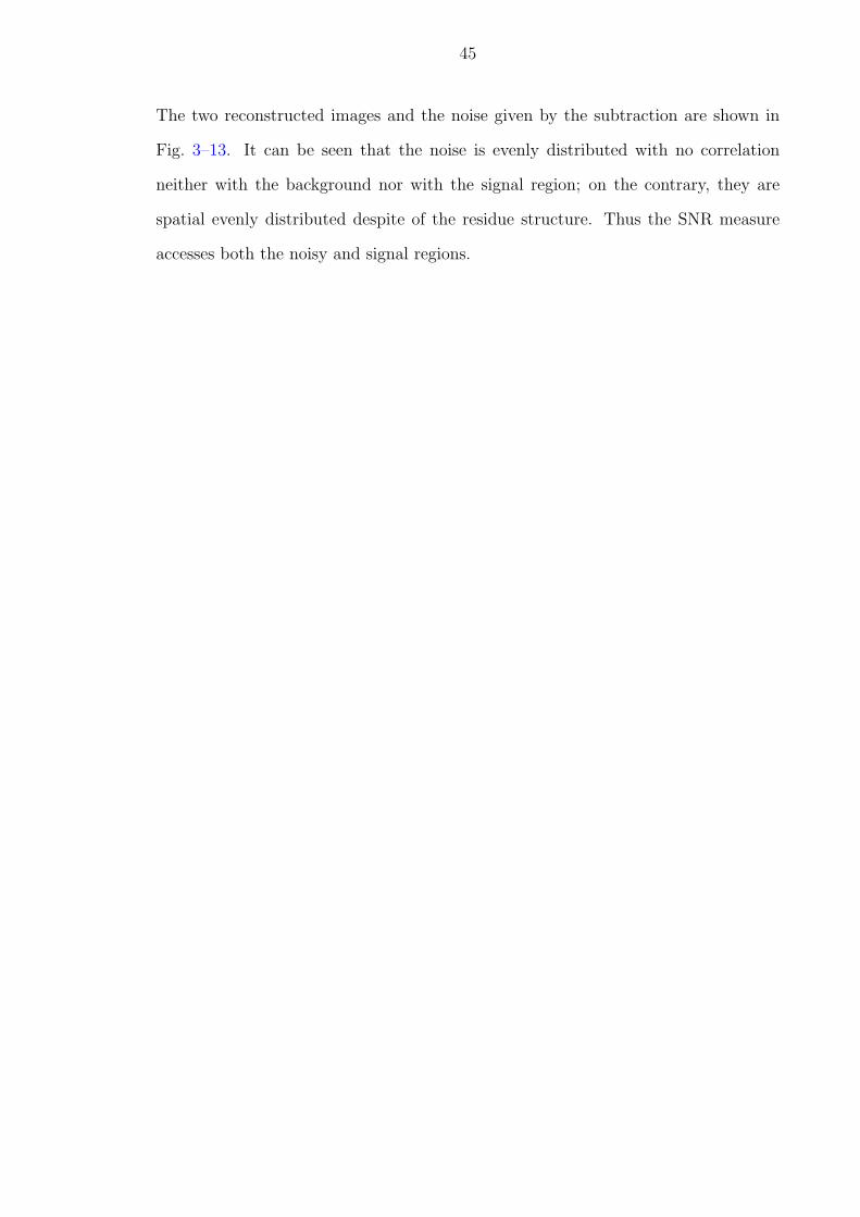
45

The two reconstructed images and the noise given by the subtraction are shown in

Fig. 3–13. It can be seen that the noise is evenly distributed with no correlation

neither with the background nor with the signal region; on the contrary, they are

spatial evenly distributed despite of the residue structure. Thus the SNR measure

accesses both the noisy and signal regions.

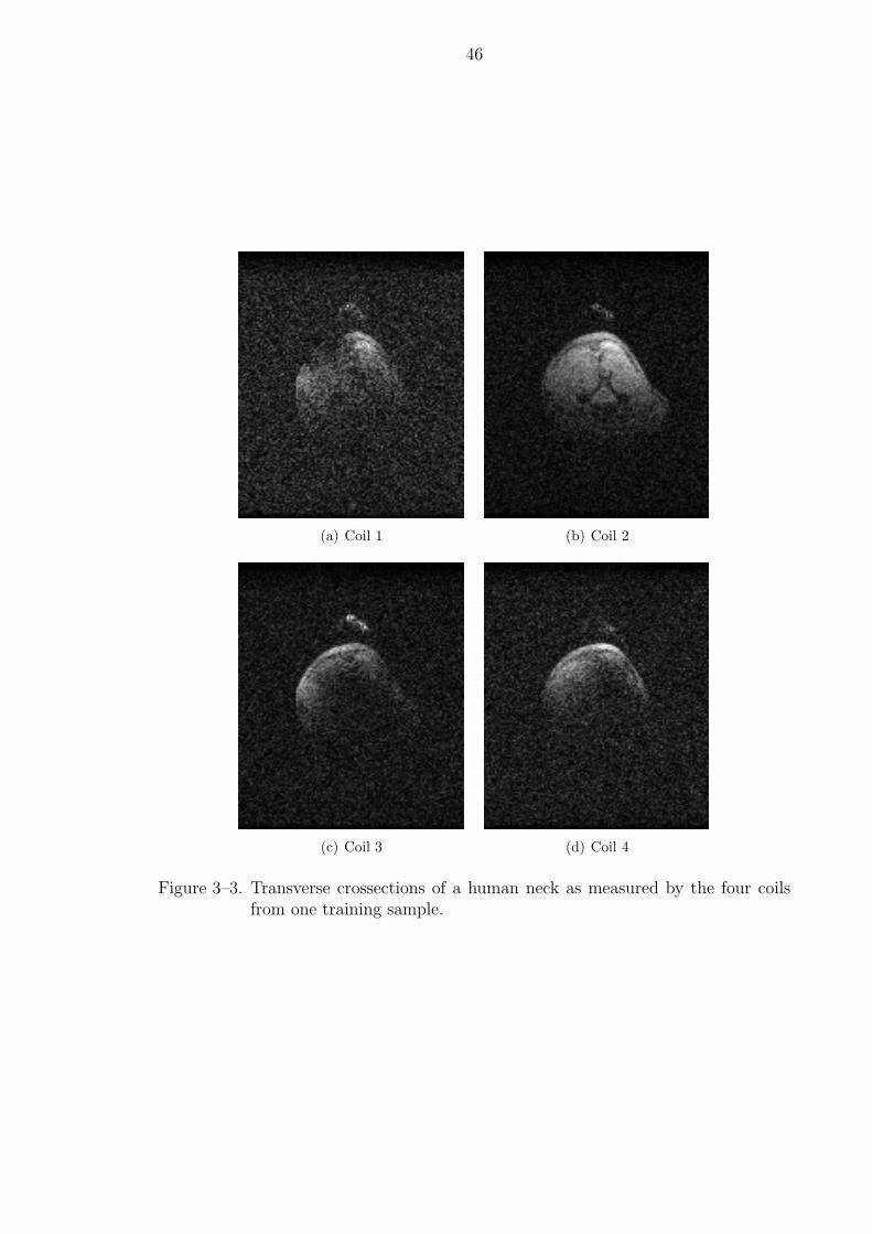
46

(a) Coil 1 (b) Coil 2

(c) Coil 3 (d) Coil 4

Figure 3–3. Transverse crossections of a human neck as measured by the four coilsfrom one training sample.

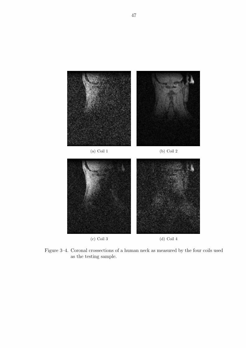
47

(a) Coil 1 (b) Coil 2

(c) Coil 3 (d) Coil 4

Figure 3–4. Coronal crossections of a human neck as measured by the four coils usedas the testing sample.

48

(a) Desire reconstructed image









(b) SNR of the desire reconstructedimage

Figure 3–5. Desired reconstructed image, (a) estimated by averaging the SoS recon-struction for each coil image sample, (b) SNR performance of the esti-mated desire.

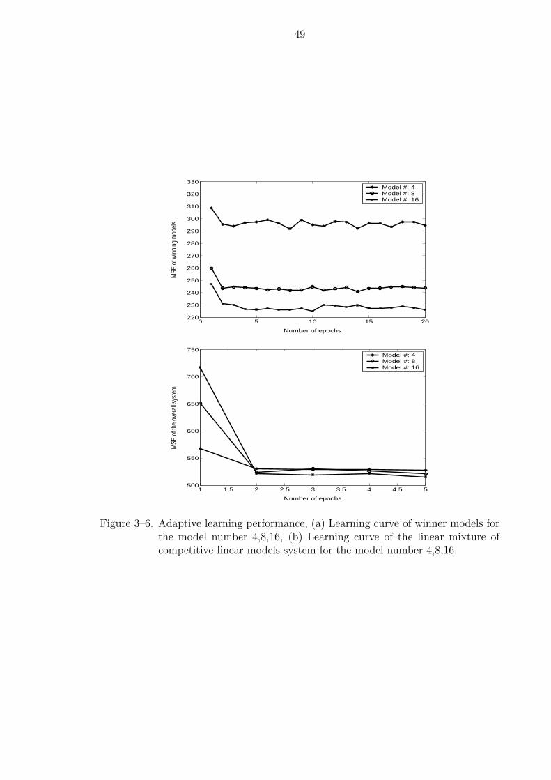
49

0 5 10 15 20220

230

240

250

260

270

280

290

300

310

320

330

MSE

of w

inni

ng m

odel

s

Number of epochs

Model #: 4Model #: 8Model #: 16

1 1.5 2 2.5 3 3.5 4 4.5 5500

550

600

650

700

750

MSE

of t

he o

vera

ll sys

tem

Number of epochs

Model #: 4Model #: 8Model #: 16

Figure 3–6. Adaptive learning performance, (a) Learning curve of winner models forthe model number 4,8,16, (b) Learning curve of the linear mixture ofcompetitive linear models system for the model number 4,8,16.

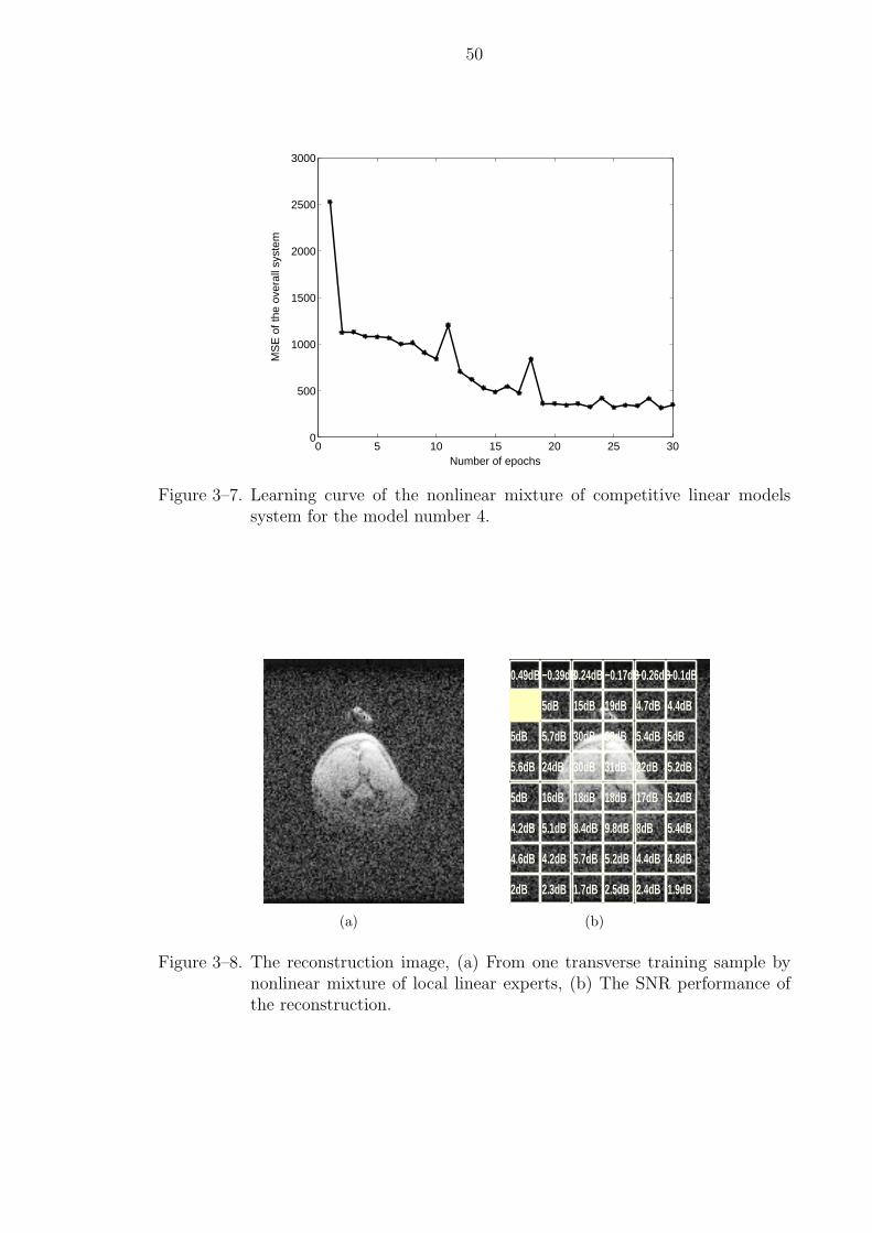
50

0 5 10 15 20 25 300

500

1000

1500

2000

2500

3000

Number of epochs

MS

E o

f the

ove

rall

syst

em

Figure 3–7. Learning curve of the nonlinear mixture of competitive linear modelssystem for the model number 4.

(a)

0.49dB −0.39dB0.24dB −0.17dB−0.26dB−0.1dB

4.5dB 5dB 15dB 19dB 4.7dB 4.4dB

5dB 5.7dB 30dB 33dB 5.4dB 5dB

5.6dB 24dB 30dB 31dB 22dB 5.2dB


4.2dB 5.1dB 8.4dB 9.8dB 8dB 5.4dB

4.6dB 4.2dB 5.7dB 5.2dB 4.4dB 4.8dB

2dB 2.3dB 1.7dB 2.5dB 2.4dB 1.9dB

(b)

Figure 3–8. The reconstruction image, (a) From one transverse training sample bynonlinear mixture of local linear experts, (b) The SNR performance ofthe reconstruction.

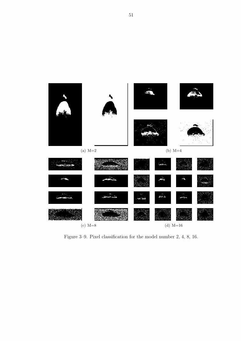
51

(a) M=2 (b) M=4

(c) M=8 (d) M=16

Figure 3–9. Pixel classification for the model number 2, 4, 8, 16.

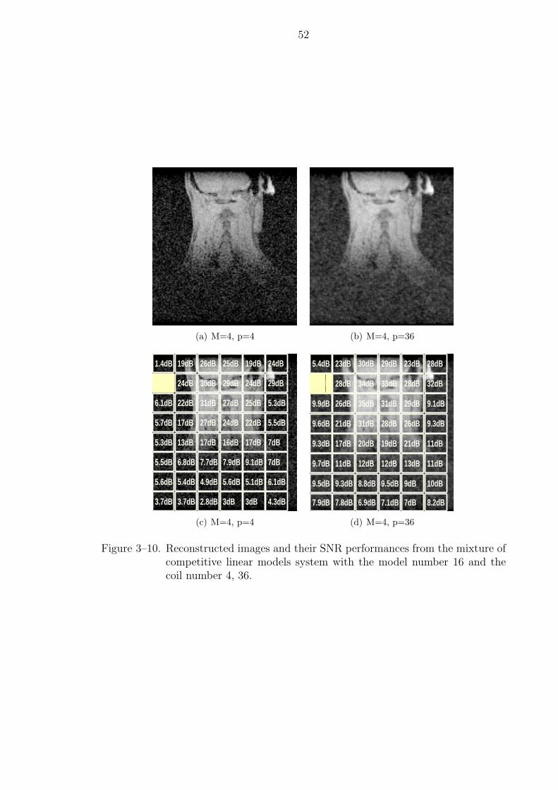
52

(a) M=4, p=4 (b) M=4, p=36



6.1dB 22dB 31dB 27dB 25dB 5.3dB

5.7dB 17dB 27dB 24dB 22dB 5.5dB


5.5dB 6.8dB 7.7dB 7.9dB 9.1dB 7dB

5.6dB 5.4dB 4.9dB 5.6dB 5.1dB 6.1dB

3.7dB 3.7dB 2.8dB 3dB 3dB 4.3dB

(c) M=4, p=4



9.9dB 26dB 35dB 31dB 29dB 9.1dB

9.6dB 21dB 31dB 28dB 26dB 9.3dB



9.5dB 9.3dB 8.8dB 9.5dB 9dB 10dB

7.9dB 7.8dB 6.9dB 7.1dB 7dB 8.2dB

(d) M=4, p=36

Figure 3–10. Reconstructed images and their SNR performances from the mixture ofcompetitive linear models system with the model number 16 and thecoil number 4, 36.

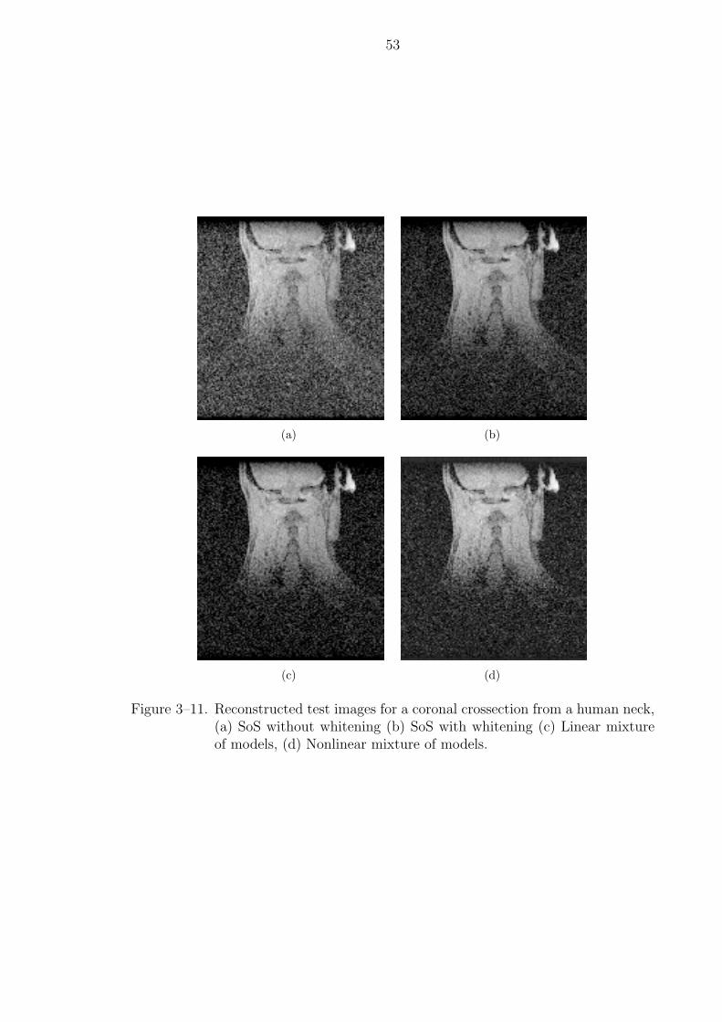
53

(a) (b)

(c) (d)

Figure 3–11. Reconstructed test images for a coronal crossection from a human neck,(a) SoS without whitening (b) SoS with whitening (c) Linear mixtureof models, (d) Nonlinear mixture of models.

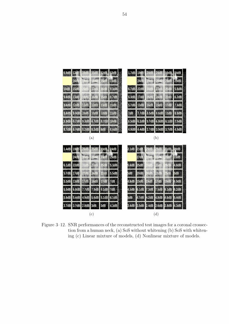
54




9.8dB 13dB 18dB 16dB 15dB 9.7dB


9.9dB 9.9dB 10dB 10dB 12dB 11dB

9.9dB 9.7dB 9.3dB 9.7dB 9.7dB 10dB

8.7dB 8.7dB 8.2dB 8.2dB 8dB 8.6dB

(a)



6.7dB 22dB 30dB 27dB 25dB 5.8dB

6.3dB 17dB 26dB 24dB 22dB 6.2dB

5.7dB 13dB 16dB 15dB 17dB 7.6dB

7dB 7.7dB 8.5dB 8.6dB 11dB 8.9dB

6.5dB 6.3dB 5.7dB 6.8dB 6.1dB 7.5dB

4.8dB 4.4dB 3.7dB 3.9dB 3.7dB 4.9dB

(b)



6.1dB 22dB 31dB 27dB 25dB 5.3dB

5.7dB 17dB 27dB 24dB 22dB 5.5dB


5.5dB 6.8dB 7.7dB 7.9dB 9.1dB 7dB

5.6dB 5.4dB 4.9dB 5.6dB 5.1dB 6.1dB

3.7dB 3.7dB 2.8dB 3dB 3dB 4.3dB

(c)



5.6dB 25dB 35dB 31dB 29dB 4.8dB


4.8dB 15dB 19dB 17dB 19dB 6.9dB

4.5dB 6.1dB 7.3dB 7.5dB 9.1dB 6.2dB

5dB 4.7dB 4.2dB 4.8dB 4.6dB 5.4dB

3.4dB 3.5dB 2.4dB 2.6dB 2.8dB 4.3dB

(d)

Figure 3–12. SNR performances of the reconstructed test images for a coronal crossec-tion from a human neck, (a) SoS without whitening (b) SoS with whiten-ing (c) Linear mixture of models, (d) Nonlinear mixture of models.

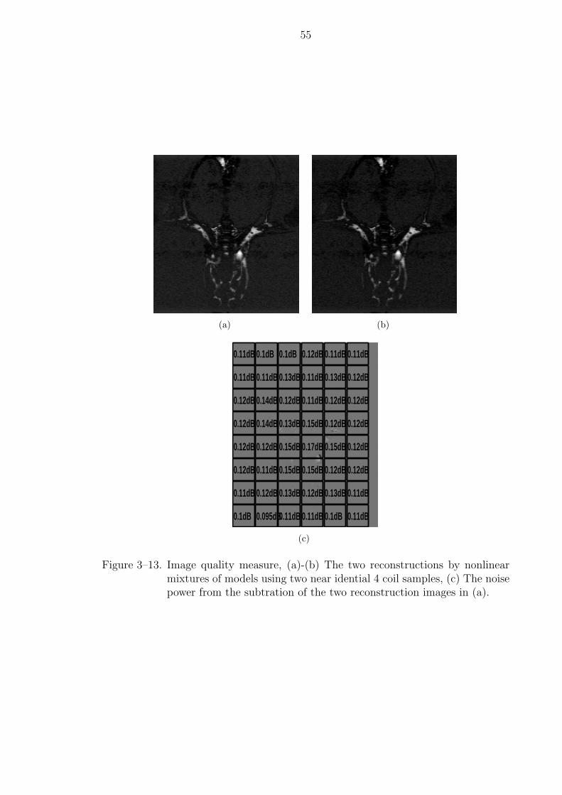
55

(a) (b)

0.11dB 0.1dB 0.1dB 0.12dB 0.11dB 0.11dB

0.11dB 0.11dB 0.13dB 0.11dB 0.13dB 0.12dB

0.12dB 0.14dB 0.12dB 0.11dB 0.12dB 0.12dB

0.12dB 0.14dB 0.13dB 0.15dB 0.12dB 0.12dB

0.12dB 0.12dB 0.15dB 0.17dB 0.15dB 0.12dB

0.12dB 0.11dB 0.15dB 0.15dB 0.12dB 0.12dB

0.11dB 0.12dB 0.13dB 0.12dB 0.13dB 0.11dB

0.1dB 0.095dB0.11dB 0.11dB 0.1dB 0.11dB

(c)

Figure 3–13. Image quality measure, (a)-(b) The two reconstructions by nonlinearmixtures of models using two near idential 4 coil samples, (c) The noisepower from the subtration of the two reconstruction images in (a).

CHAPTER 4SUPERVISED LEARNING IN ADAPTIVE IMAGE RECONSTRUCTION

METHODS, PART B: INFORMATION THEORETIC LEARNING (ITL) OFMIXTURE OF LOCAL LINEAR EXPERTS

4.1 Brief Review of Information Theoretic Learning (ITL)

In the last chapter, the nonlinear competitive local linear experts network esti-

mates the reconstruction image by combining the outputs from the multiple linear

model by a multilayer perceptron (MLP). This nonlinear combination is superior to

the linear combination due to its nonlinear compression to the models which don’t

win the adaptations. The training for the MLP weights is based on minimizing mean

square error (MSE) criterion. This criterion is extensively applied in the training of

linear or nonlinear systems due to its mathematical simplicity and practicability. It is

based on the assumption that the second order statistics is sufficient to represent the

data distribution. This is often true since the probability density distributions (pdfs)

of many systems exhibits Gaussianity, where their pdfs are exactly determined by

mean and variance. Besides, Gaussianity is also supported by the central limit theo-

rem for a large amount of sample number. However, neural networks don’t necessarily

confine the moments of their output error to the first and second order statistics due

to the implicit nonlinear processing elements (PEs), which is true for generalized

nonlinear networks. Thus, minimizing MSE might not be sufficient to capture all the

information used to train the network.

As we know, entropy is used to measure the uncertainty of a random variable due

to a its pdf. Shannon firstly defined the average information of a random variable,

named Shannon entropy, which is formulated in

Hs(x) = −E[log f(x)] (4–1)

56

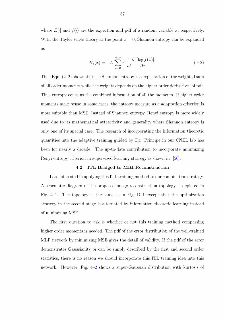
57

where E[·] and f(·) are the expection and pdf of a random variable x, respectively.

With the Taylor series theory at the point x = 0, Shannon entropy can be expanded

as

Hs(x) = −E[+∞∑n=0

xn 1

n!

∂n[log f(x)]

∂x] (4–2)

Thus Eqn. (4–2) shows that the Shannon entropy is a expectation of the weighted sum

of all order moments while the weights depends on the higher order derivatives of pdf.

Thus entropy contains the combined information of all the moments. If higher order

moments make sense in some cases, the entropy measure as a adaptation criterion is

more suitable than MSE. Instead of Shannon entropy, Renyi entropy is more widely

used due to its mathematical attractivity and generality where Shannon entropy is

only one of its special case. The research of incorporating the information theoretic

quantities into the adaptive training guided by Dr. Principe in our CNEL lab has

been for nearly a decade. The up-to-date contribution to incorporate minimizing

Renyi entropy criterion in supervised learning strategy is shown in [56].

4.2 ITL Bridged to MRI Reconstruction

I are interested in applying this ITL training method to our combination strategy.

A schematic diagram of the proposed image reconstruction topology is depicted in

Fig. 4–1. The topology is the same as in Fig. D–1 except that the optimization

strategy in the second stage is alternated by information theoretic learning instead

of minimizing MSE.

The first question to ask is whether or not this training method compassing

higher order moments is needed. The pdf of the error distribution of the well-trained

MLP network by minimizing MSE gives the detail of validity. If the pdf of the error

demonstrates Gaussianity or can be simply described by the first and second order

statistics, there is no reason we should incorporate this ITL training idea into this

network. However, Fig. 4–2 shows a super-Gaussian distribution with kurtosis of

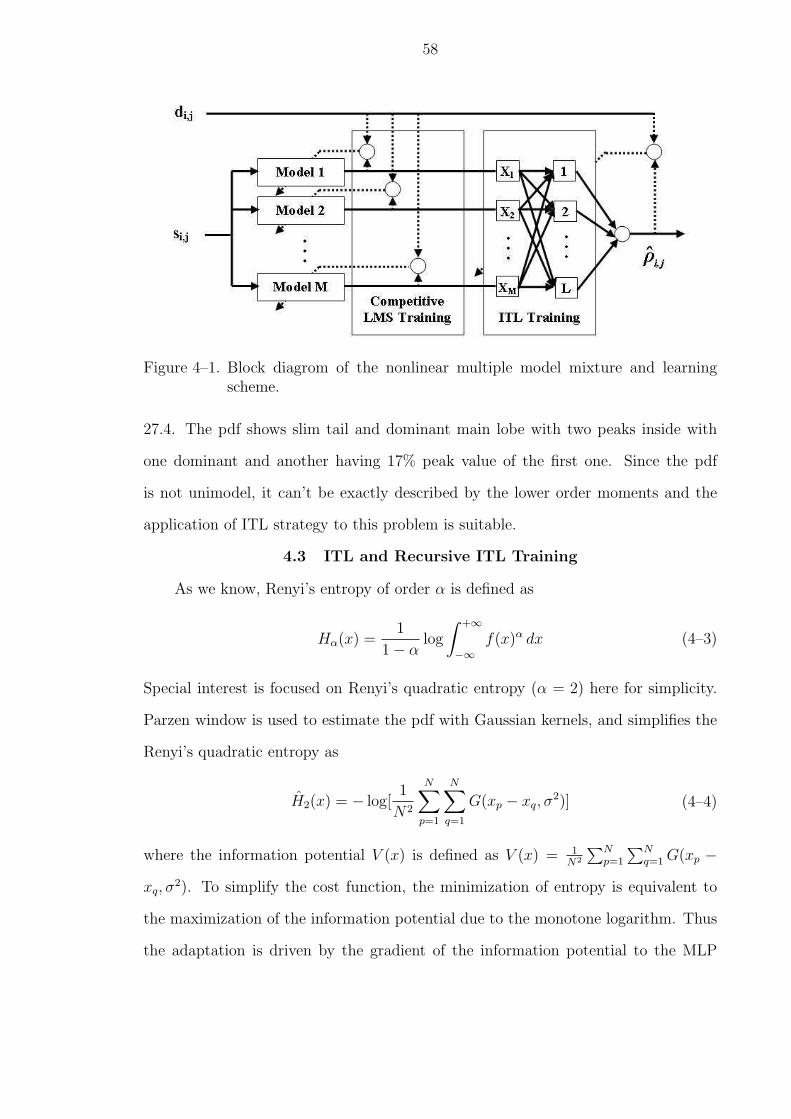
58

Figure 4–1. Block diagrom of the nonlinear multiple model mixture and learningscheme.

27.4. The pdf shows slim tail and dominant main lobe with two peaks inside with

one dominant and another having 17% peak value of the first one. Since the pdf

is not unimodel, it can’t be exactly described by the lower order moments and the

application of ITL strategy to this problem is suitable.

4.3 ITL and Recursive ITL Training

As we know, Renyi’s entropy of order α is defined as

Hα(x) =1

1− αlog

∫ +∞

−∞f(x)α dx (4–3)

Special interest is focused on Renyi’s quadratic entropy (α = 2) here for simplicity.

Parzen window is used to estimate the pdf with Gaussian kernels, and simplifies the

Renyi’s quadratic entropy as

H2(x) = − log[1

N2

N∑p=1

N∑q=1

G(xp − xq, σ2)] (4–4)

where the information potential V (x) is defined as V (x) = 1N2

∑Np=1

∑Nq=1 G(xp −

xq, σ2). To simplify the cost function, the minimization of entropy is equivalent to

the maximization of the information potential due to the monotone logarithm. Thus

the adaptation is driven by the gradient of the information potential to the MLP

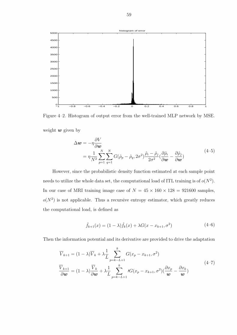
59

−1 −0.8 −0.6 −0.4 −0.2 0 0.2 0.4 0.6 0.8 10

500

1000

1500

2000

2500

3000

3500

4000

4500

5000histogram of error

Figure 4–2. Histogram of output error from the well-trained MLP network by MSE.

weight w given by

∆w = −η∂V

∂w

= η1

N2

N∑p=1

N∑q=1

G(ρp − ρq, 2σ2)

ρi − ρj

2σ2(∂ρi

∂w− ∂ρj

∂w)

(4–5)

However, since the probabilistic density function estimated at each sample point

needs to utilize the whole data set, the computational load of ITL training is of o(N2).

In our case of MRI training image case of N = 45 × 160 × 128 = 921600 samples,

o(N2) is not applicable. Thus a recursive entropy estimator, which greatly reduces

the computational load, is defined as

fk+1(x) = (1− λ)fk(x) + λG(x− xk+1, σ2) (4–6)

Then the information potential and its derivative are provided to drive the adaptation

V k+1 = (1− λ)V k + λ1

L

k∑

p=k−L+1

G(xp − xk+1, σ2)

V k+1

∂w= (1− λ)

V k

∂w+ λ

1

L

k∑

p=k−L+1

′G(xp − xk+1, σ2)(

∂xp

w− ∂xk

w)

(4–7)

60

0 50 100 1500

0.1

0.2

0.3

0.4

0.5

0.6

0.7Learning curve

# of epoch

V

(a)

0 50 100 1500

0.01

0.02

0.03

0.04

0.05

0.06

0.07

0.08

0.09

0.1kernel variance

Number of epoch

Ke

rne

l siz

e

(b)

Figure 4–3. Adaptive learning performance, (a) The information potential learningcurve, (b) The kernel variance anealing curve.

Thus the computational load of the recursive ITL training greatly reduce to o(NL),

where

In the MRI reconstruction problem, suppose forgetting length L = 20, the com-

putational load is o(NL) = o(921600 × 20) = o(18432000). Considering that the

algorithm needs a large number of epochs (for example, 150 epochs), the matlab code

still takes a long time. Fortunately, matlab provides inferfaces to external routines

written in other languages, called MATLAB Application Program Interface. Specifi-

cally, the C engine routine allows calling the components of a C MEX-file. Thus the

recursive ITL code was written in C and based on an self-defined interface function,

matlab can call this core code in C to greatly save computational time. Though the

ITL code consists lots of matrix computation, this CMEX code uses only approxi-

mately 1/20 execution time, which makes the code feasible.

4.4 Results

The performance of the proposed ITL training method is also demonstrated in

phased-array MRI reconstruction using transverse (45 measurements) and coronal (9

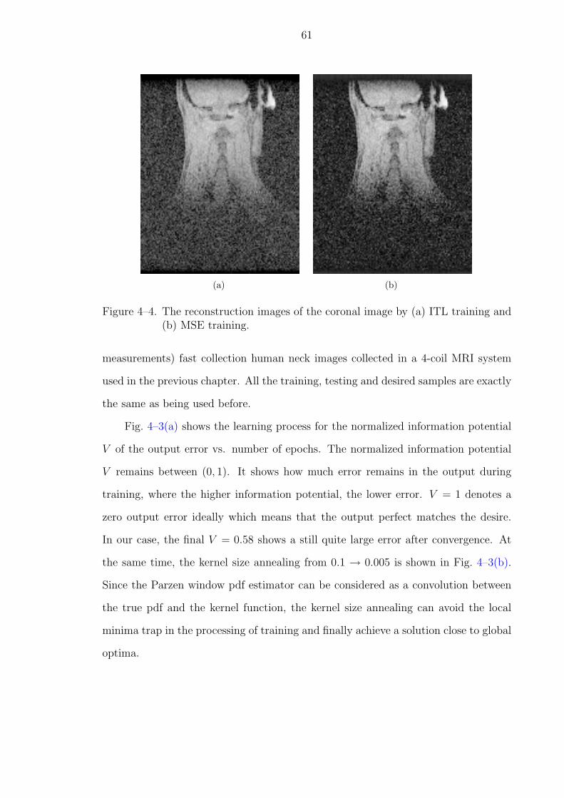
61

(a) (b)

Figure 4–4. The reconstruction images of the coronal image by (a) ITL training and(b) MSE training.

measurements) fast collection human neck images collected in a 4-coil MRI system

used in the previous chapter. All the training, testing and desired samples are exactly

the same as being used before.

Fig. 4–3(a) shows the learning process for the normalized information potential

V of the output error vs. number of epochs. The normalized information potential

V remains between (0, 1). It shows how much error remains in the output during

training, where the higher information potential, the lower error. V = 1 denotes a

zero output error ideally which means that the output perfect matches the desire.

In our case, the final V = 0.58 shows a still quite large error after convergence. At

the same time, the kernel size annealing from 0.1 → 0.005 is shown in Fig. 4–3(b).

Since the Parzen window pdf estimator can be considered as a convolution between

the true pdf and the kernel function, the kernel size annealing can avoid the local

minima trap in the processing of training and finally achieve a solution close to global

optima.

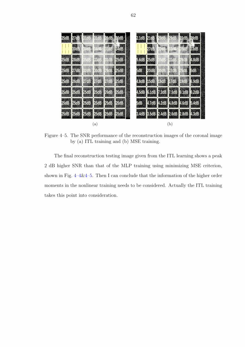
62









(a)



5.6dB 25dB 35dB 31dB 29dB 4.8dB


4.8dB 15dB 19dB 17dB 19dB 6.9dB

4.5dB 6.1dB 7.3dB 7.5dB 9.1dB 6.2dB

5dB 4.7dB 4.2dB 4.8dB 4.6dB 5.4dB

3.4dB 3.5dB 2.4dB 2.6dB 2.8dB 4.3dB

(b)

Figure 4–5. The SNR performance of the reconstruction images of the coronal imageby (a) ITL training and (b) MSE training.

The final reconstruction testing image given from the ITL learning shows a peak

2 dB higher SNR than that of the MLP training using minimizing MSE criterion,

shown in Fig. 4–4&4–5. Then I can conclude that the information of the higher order

moments in the nonlinear training needs to be considered. Actually the ITL training

takes this point into consideration.

CHAPTER 5UNSUPERVISED LEARNING IN fMRI TEMPORAL ACTIVATION PATTERN

CLASSIFICATION

5.1 Brief Review of fMRI

The interest in understanding brain functions dates back to several centuries

ago. But it was Gall et. al who argued for the first time that functional modules are

localized at specified regions and correlated to particular tasks [57]. However, it was

only in the last decade that the rapid development of functional magnetic resonance

imaging (fMRI) techniques allowed dynamic mapping of the brain processes with fine

spatial resolution. The information between functional brain regions and cognitive

processes has being investigated [7], and the temporal segmented activity demon-

strates functional independence with respect to the localized brain anatomy [8]. So

far the main methodology in fMRI is to segment the activation region in terms of the

temporal response given by the external periodic stimulus. Such stimulus alternates

between task and control conditions giving a supervised baseline for the temporal

response. Plenty of methods have been proposed to address this problem, which can

be roughly categorized into model-based and model-independent. Correlation analy-

sis (CA), as a model-based method [58, 59], combines the subspace modeling of the

hemodynamic response and the use of the spatial information to analyze fMRI series.

However, the model-based methods are not effective in neuronal pattern analysis when

the temporal information is not available. Thus various model-independent methods

were proposed, including principal component analysis (PCA) [60, 61], independent

component analysis (ICA) [62, 63] and clustering methods [64, 65, 66] to quantify the

fMRI responses.

63

64

However the challenge remains in localizing brain function when there is no a

priori knowledge available about the time window in which a stimulus may elicit a re-

sponse [67, 68]. In such cases there’s no timing for the brain response, so conventional

segmentation with stimulus is impossible. In addition, the fMRI signal is subject to

high level of noise, especially for non-repeatable physiological events or relatively long

events (compared to cognitive processes) in the brain, such as those following eating

and drinking. A temporal clustering analysis (TCA) method was proposed to reveal

the brain response following eating [9]. This is a space-time methodology that tries to

bridge the gap between spatial localizations and temporal responses. However, TCA

can still be improved and its performance is hampered by several assumptions that

are not necessarily satisfied by cognitive signals measured by fMRI. New methods are

required for dealing with these challenges.

Subspace projection method as used in the image deconvolution seems to be suit-

able for this task. They have the advantage of data compression and noise cancelation

and are widely implemented in image processing, such as image compression [69], hy-

perspectral image classification [70], etc. The optimal linear subspace projection in

terms of preserving energy is the well known principal component analysis (PCA) [71].

However, in many cases the global PCA is not optimal in particular when the data dis-

tributions are far from Gaussian. Competitive learning is known for its powerful local

feature extraction as demonstrated in the later chapters of this dissertation. It can

also be applied in unsupervised mode as in vector quantization combined with PCA

[72, 73]. Haykin et al. proposed the OIAL (optimally integrated adaptive learning)

method, which gives smaller MSE and higher compression ratio [74]. However, OIAL

doesn’t take the bias among models into consideration, which leads to sub-optimal

results. Fancourt et al. combined the mixture of experts and PCA into a cooperative

network to segment time series and images [75]. Both methods are sensitive to the

initial condition especially when input is in a high dimensional space. The SOM

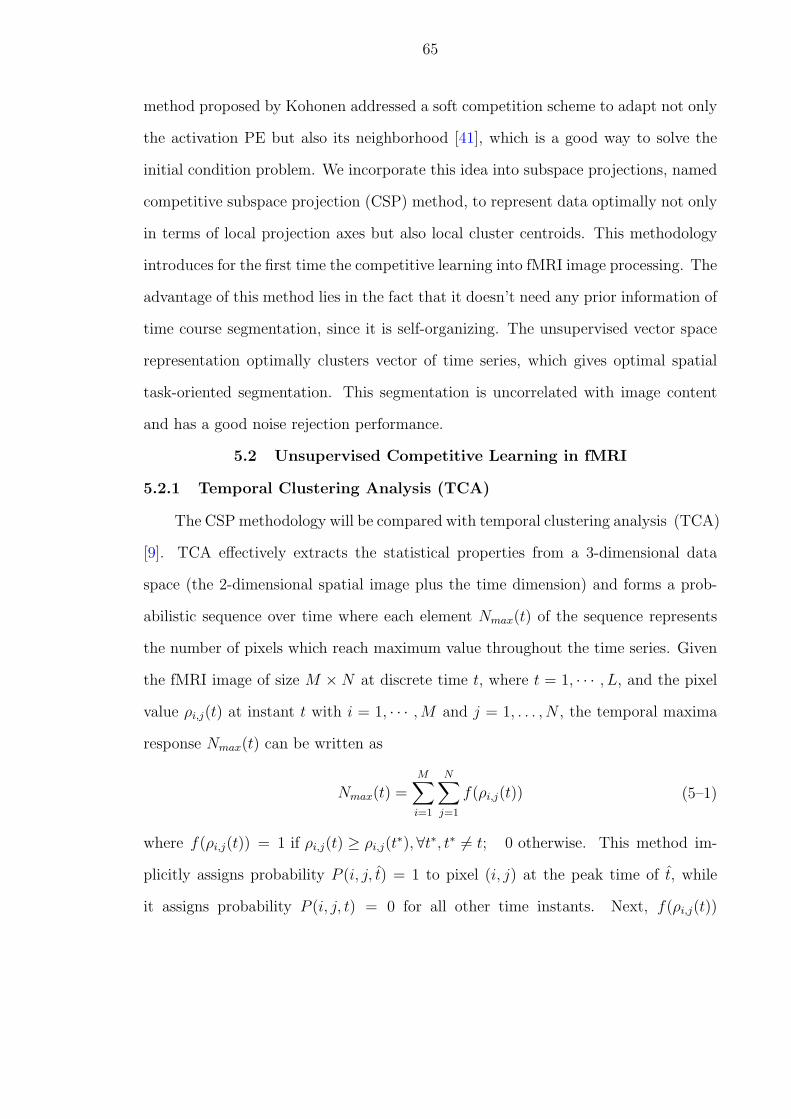
65

method proposed by Kohonen addressed a soft competition scheme to adapt not only

the activation PE but also its neighborhood [41], which is a good way to solve the

initial condition problem. We incorporate this idea into subspace projections, named

competitive subspace projection (CSP) method, to represent data optimally not only

in terms of local projection axes but also local cluster centroids. This methodology

introduces for the first time the competitive learning into fMRI image processing. The

advantage of this method lies in the fact that it doesn’t need any prior information of

time course segmentation, since it is self-organizing. The unsupervised vector space

representation optimally clusters vector of time series, which gives optimal spatial

task-oriented segmentation. This segmentation is uncorrelated with image content

and has a good noise rejection performance.

5.2 Unsupervised Competitive Learning in fMRI

5.2.1 Temporal Clustering Analysis (TCA)

The CSP methodology will be compared with temporal clustering analysis (TCA)

[9]. TCA effectively extracts the statistical properties from a 3-dimensional data

space (the 2-dimensional spatial image plus the time dimension) and forms a prob-

abilistic sequence over time where each element Nmax(t) of the sequence represents

the number of pixels which reach maximum value throughout the time series. Given

the fMRI image of size M ×N at discrete time t, where t = 1, · · · , L, and the pixel

value ρi,j(t) at instant t with i = 1, · · · ,M and j = 1, . . . , N , the temporal maxima

response Nmax(t) can be written as

Nmax(t) =M∑i=1

N∑j=1

f(ρi,j(t)) (5–1)

where f(ρi,j(t)) = 1 if ρi,j(t) ≥ ρi,j(t∗),∀t∗, t∗ 6= t; 0 otherwise. This method im-

plicitly assigns probability P (i, j, t) = 1 to pixel (i, j) at the peak time of t, while

it assigns probability P (i, j, t) = 0 for all other time instants. Next, f(ρi,j(t))

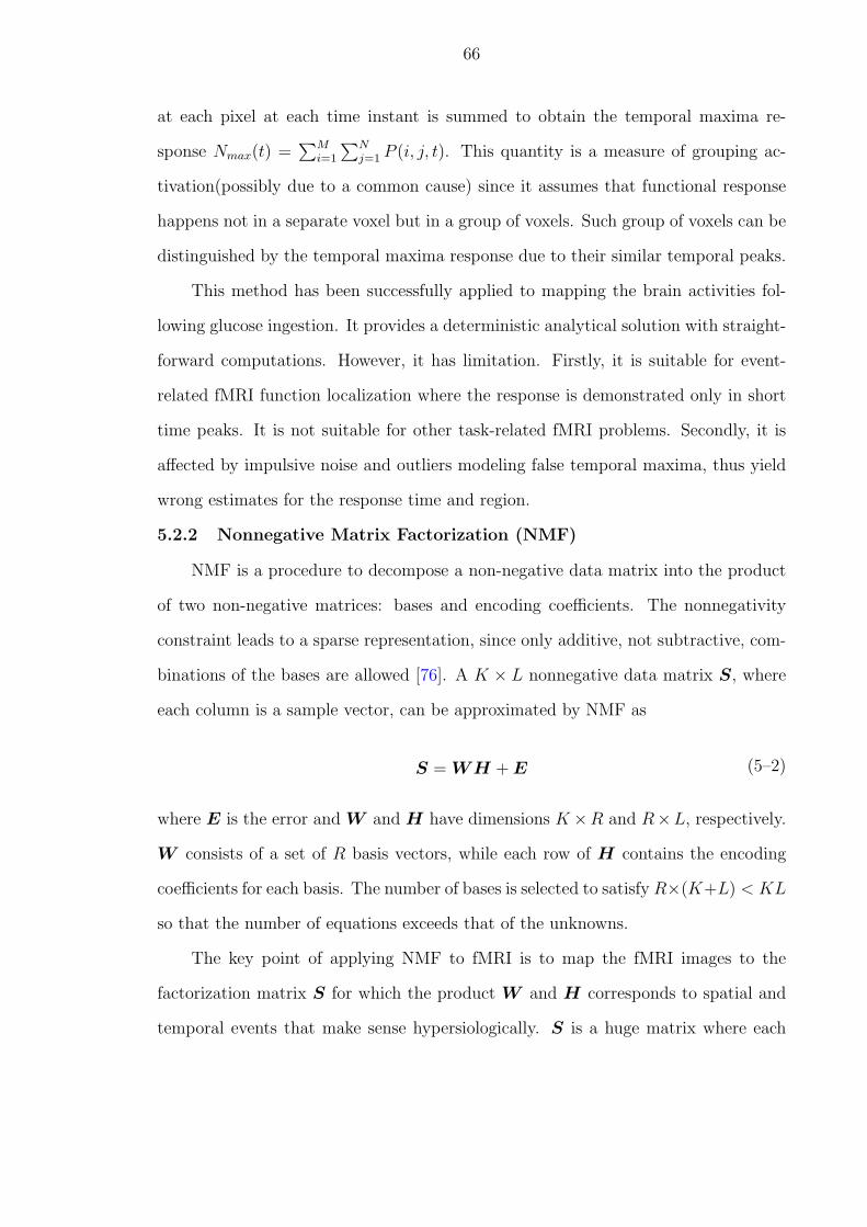
66

at each pixel at each time instant is summed to obtain the temporal maxima re-

sponse Nmax(t) =∑M

i=1

∑Nj=1 P (i, j, t). This quantity is a measure of grouping ac-

tivation(possibly due to a common cause) since it assumes that functional response

happens not in a separate voxel but in a group of voxels. Such group of voxels can be

distinguished by the temporal maxima response due to their similar temporal peaks.

This method has been successfully applied to mapping the brain activities fol-

lowing glucose ingestion. It provides a deterministic analytical solution with straight-

forward computations. However, it has limitation. Firstly, it is suitable for event-

related fMRI function localization where the response is demonstrated only in short

time peaks. It is not suitable for other task-related fMRI problems. Secondly, it is

affected by impulsive noise and outliers modeling false temporal maxima, thus yield

wrong estimates for the response time and region.

5.2.2 Nonnegative Matrix Factorization (NMF)

NMF is a procedure to decompose a non-negative data matrix into the product

of two non-negative matrices: bases and encoding coefficients. The nonnegativity

constraint leads to a sparse representation, since only additive, not subtractive, com-

binations of the bases are allowed [76]. A K × L nonnegative data matrix S, where

each column is a sample vector, can be approximated by NMF as

S = WH + E (5–2)

where E is the error and W and H have dimensions K ×R and R×L, respectively.

W consists of a set of R basis vectors, while each row of H contains the encoding

coefficients for each basis. The number of bases is selected to satisfy R×(K+L) < KL

so that the number of equations exceeds that of the unknowns.

The key point of applying NMF to fMRI is to map the fMRI images to the

factorization matrix S for which the product W and H corresponds to spatial and

temporal events that make sense hypersiologically. S is a huge matrix where each

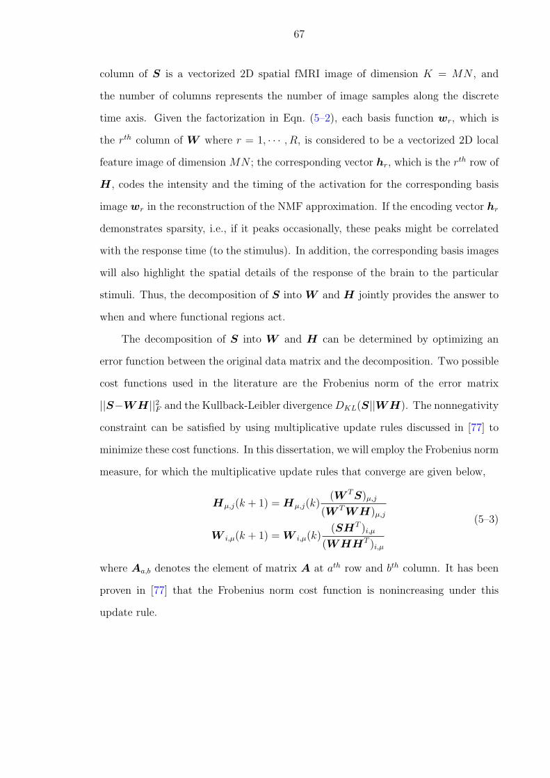
67

column of S is a vectorized 2D spatial fMRI image of dimension K = MN , and

the number of columns represents the number of image samples along the discrete

time axis. Given the factorization in Eqn. (5–2), each basis function wr, which is

the rth column of W where r = 1, · · · , R, is considered to be a vectorized 2D local

feature image of dimension MN ; the corresponding vector hr, which is the rth row of

H , codes the intensity and the timing of the activation for the corresponding basis

image wr in the reconstruction of the NMF approximation. If the encoding vector hr

demonstrates sparsity, i.e., if it peaks occasionally, these peaks might be correlated

with the response time (to the stimulus). In addition, the corresponding basis images

will also highlight the spatial details of the response of the brain to the particular

stimuli. Thus, the decomposition of S into W and H jointly provides the answer to

when and where functional regions act.

The decomposition of S into W and H can be determined by optimizing an

error function between the original data matrix and the decomposition. Two possible

cost functions used in the literature are the Frobenius norm of the error matrix

||S−WH ||2F and the Kullback-Leibler divergence DKL(S||WH). The nonnegativity

constraint can be satisfied by using multiplicative update rules discussed in [77] to

minimize these cost functions. In this dissertation, we will employ the Frobenius norm

measure, for which the multiplicative update rules that converge are given below,

Hµ,j(k + 1) = Hµ,j(k)(W T S)µ,j

(W T WH)µ,j

W i,µ(k + 1) = W i,µ(k)(SHT )i,µ

(WHHT )i,µ

(5–3)

where Aa,b denotes the element of matrix A at ath row and bth column. It has been

proven in [77] that the Frobenius norm cost function is nonincreasing under this

update rule.

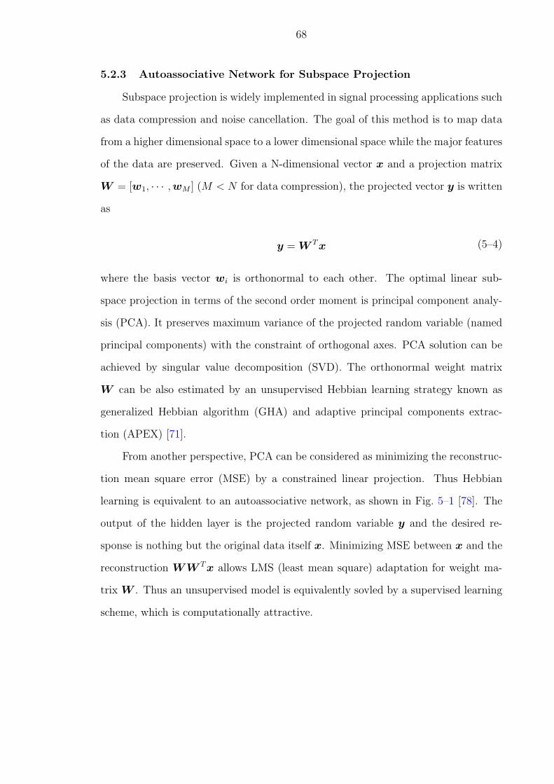
68

5.2.3 Autoassociative Network for Subspace Projection

Subspace projection is widely implemented in signal processing applications such

as data compression and noise cancellation. The goal of this method is to map data

from a higher dimensional space to a lower dimensional space while the major features

of the data are preserved. Given a N-dimensional vector x and a projection matrix

W = [w1, · · · , wM ] (M < N for data compression), the projected vector y is written

as

y = W T x (5–4)

where the basis vector wi is orthonormal to each other. The optimal linear sub-

space projection in terms of the second order moment is principal component analy-

sis (PCA). It preserves maximum variance of the projected random variable (named

principal components) with the constraint of orthogonal axes. PCA solution can be

achieved by singular value decomposition (SVD). The orthonormal weight matrix

W can be also estimated by an unsupervised Hebbian learning strategy known as

generalized Hebbian algorithm (GHA) and adaptive principal components extrac-

tion (APEX) [71].

From another perspective, PCA can be considered as minimizing the reconstruc-

tion mean square error (MSE) by a constrained linear projection. Thus Hebbian

learning is equivalent to an autoassociative network, as shown in Fig. 5–1 [78]. The

output of the hidden layer is the projected random variable y and the desired re-

sponse is nothing but the original data itself x. Minimizing MSE between x and the

reconstruction WW T x allows LMS (least mean square) adaptation for weight ma-

trix W . Thus an unsupervised model is equivalently sovled by a supervised learning

scheme, which is computationally attractive.

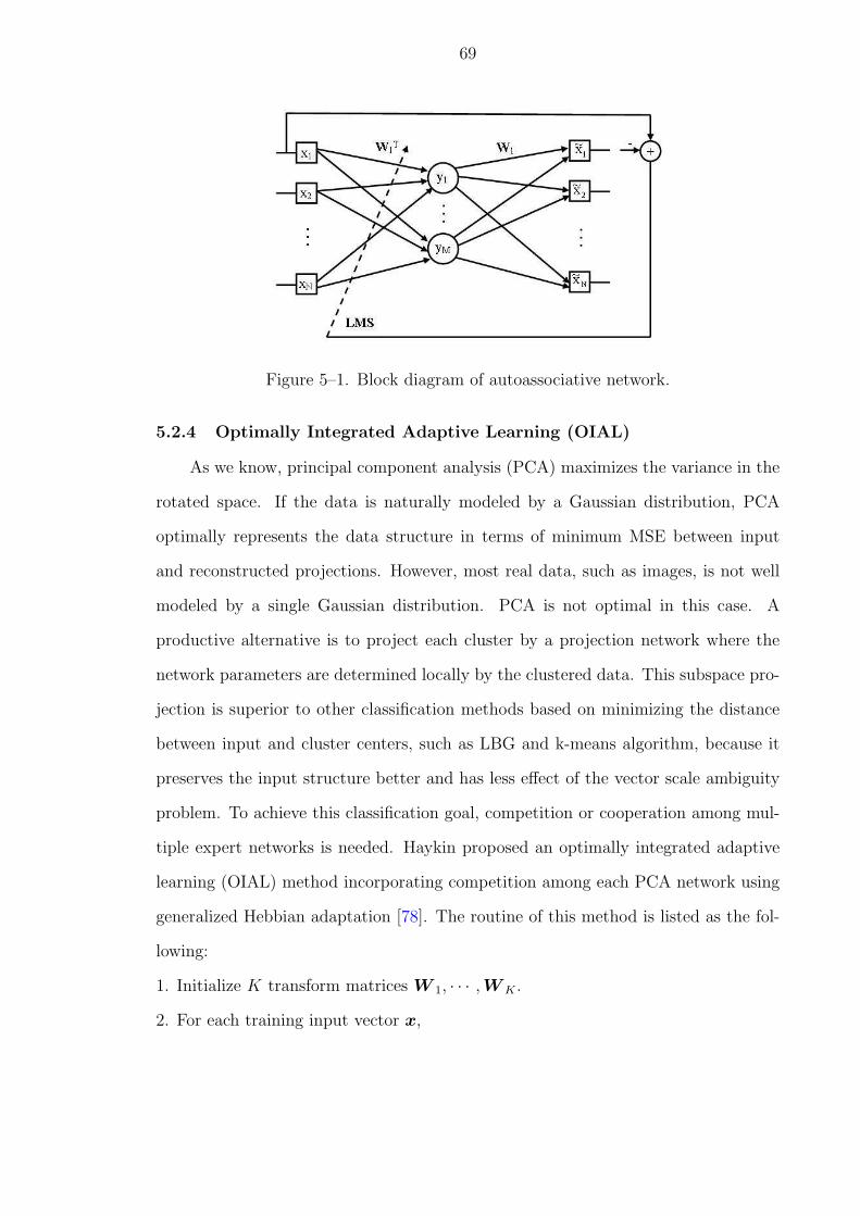
69

Figure 5–1. Block diagram of autoassociative network.

5.2.4 Optimally Integrated Adaptive Learning (OIAL)

As we know, principal component analysis (PCA) maximizes the variance in the

rotated space. If the data is naturally modeled by a Gaussian distribution, PCA

optimally represents the data structure in terms of minimum MSE between input

and reconstructed projections. However, most real data, such as images, is not well

modeled by a single Gaussian distribution. PCA is not optimal in this case. A

productive alternative is to project each cluster by a projection network where the

network parameters are determined locally by the clustered data. This subspace pro-

jection is superior to other classification methods based on minimizing the distance

between input and cluster centers, such as LBG and k-means algorithm, because it

preserves the input structure better and has less effect of the vector scale ambiguity

problem. To achieve this classification goal, competition or cooperation among mul-

tiple expert networks is needed. Haykin proposed an optimally integrated adaptive

learning (OIAL) method incorporating competition among each PCA network using

generalized Hebbian adaptation [78]. The routine of this method is listed as the fol-

lowing:

1. Initialize K transform matrices W 1, · · · ,W K .

2. For each training input vector x,

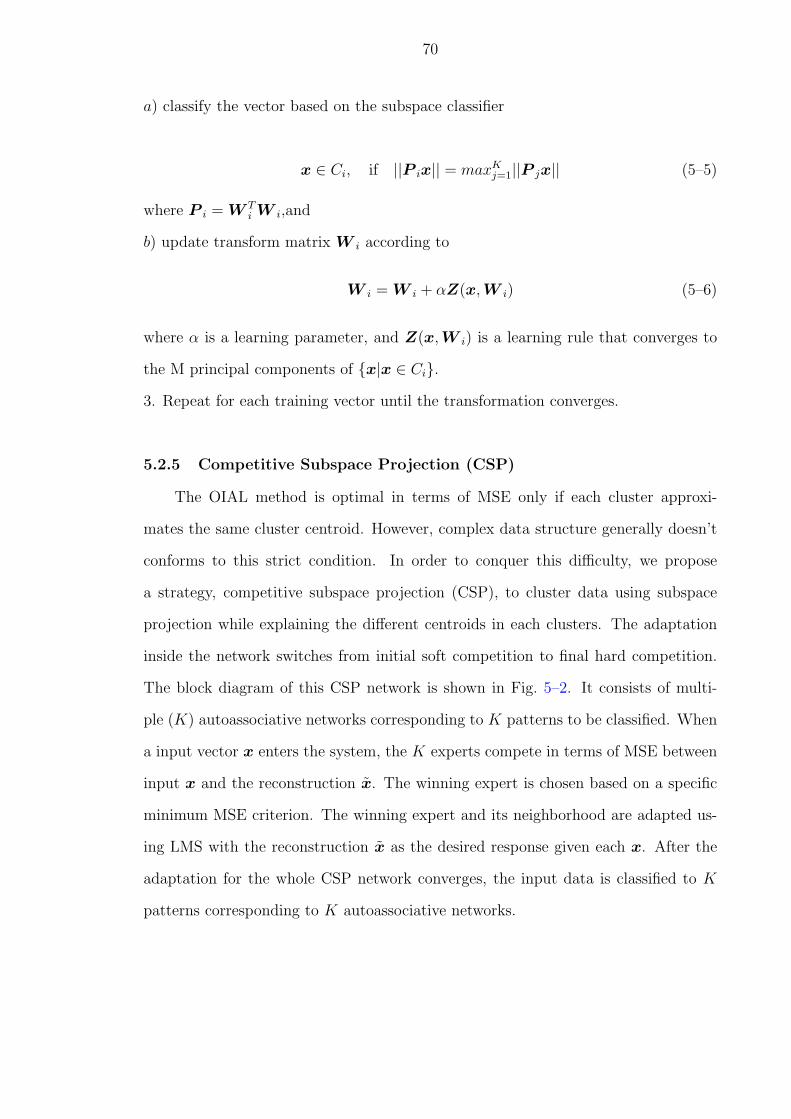
70

a) classify the vector based on the subspace classifier

x ∈ Ci, if ||P ix|| = maxKj=1||P jx|| (5–5)

where P i = W Ti W i,and

b) update transform matrix W i according to

W i = W i + αZ(x,W i) (5–6)

where α is a learning parameter, and Z(x,W i) is a learning rule that converges to

the M principal components of x|x ∈ Ci.3. Repeat for each training vector until the transformation converges.

5.2.5 Competitive Subspace Projection (CSP)

The OIAL method is optimal in terms of MSE only if each cluster approxi-

mates the same cluster centroid. However, complex data structure generally doesn’t

conforms to this strict condition. In order to conquer this difficulty, we propose

a strategy, competitive subspace projection (CSP), to cluster data using subspace

projection while explaining the different centroids in each clusters. The adaptation

inside the network switches from initial soft competition to final hard competition.

The block diagram of this CSP network is shown in Fig. 5–2. It consists of multi-

ple (K) autoassociative networks corresponding to K patterns to be classified. When

a input vector x enters the system, the K experts compete in terms of MSE between

input x and the reconstruction x. The winning expert is chosen based on a specific

minimum MSE criterion. The winning expert and its neighborhood are adapted us-

ing LMS with the reconstruction x as the desired response given each x. After the

adaptation for the whole CSP network converges, the input data is classified to K

patterns corresponding to K autoassociative networks.

71

Figure 5–2. The block diagram of competitive subspace projection methodology.

5.2.5.1 hard competition

The competition strategy is denoted as hard competition if only a single ex-

pert with the least MSE is chosen as the winner. The network architecture and

its optimization methodology with hard competition are described as follows. Each

autoassociative network explains one cluster centroid by introducing bias either to

the hidden layer or output layer, while the bias is simultaneously adapted with the

projection matrices. The bias on the output layer is preferred due to its mathe-

matical simplicity. Thus the cost function J(W , b) for each expert consists of two

partsJ(W , b) = J1(W , b)−λJ2(W ), where J1(W , b) defines the cost function sur-

face and J2(W ) is the orthogonality constraint with weighting factor λ. The two

72

items J1(W , b) and J2(W ) are given by

J1(W , b) =1

2||x− x||2

=1

2(||x||2 − 2xT WW T x + xT WW T WW T x

+ 2xT WW T b− 2xT b + bT b)

J2(W ) =M∑i=1

||wi||2 −M∑

j=1,j 6=i

[wTi wj]

(5–7)

where x is the input vector containing neighborhood pixels, x = Wy+b = WW T x+

b is the reconstruction, y = W T x is the projection vector which has less dimension

than that of x and wi is the ith column vector of matrix W . Based on the ma-

trix lemma of ∂aT a/∂w = 2J(a,w)a where J i,j(a, w) = ∂aj/∂wi, the adaptation

criterion at the nth iteration is written as

∆wi(n) =η[yi(n)(x(n)− x(n)) + x(n)(wi(n)T x(n)− yi(n))

+ λ(2wi(n)−M∑

j=1,j 6=i

P (wi,wj)wj(n))]

∆b(n) =η[x(n)− x(n)]

(5–8)

where P (wi,wj) is M × M matrix with P r,s(wi, wj) = 0 if r 6= s;

P r,s(wi,wj) = sign(wi(r) ∗ wj(r)) if r = s. sign(·) is a sign function and

r, s = 0, · · · ,M − 1.

We notice that the length of the projection vector y is less than the vector length

of x due to its subspace dimension compression. This dimension reduction results in

the error between the input x and the reconstruction x, where it is the error which

drives the adaptation. A full space projection in y causes error zero and makes no

sense for reconstruction.

5.2.5.2 soft competition

The initial condition for hard competition is a tough issue. Several options in

choosing the initial W and b are the following:

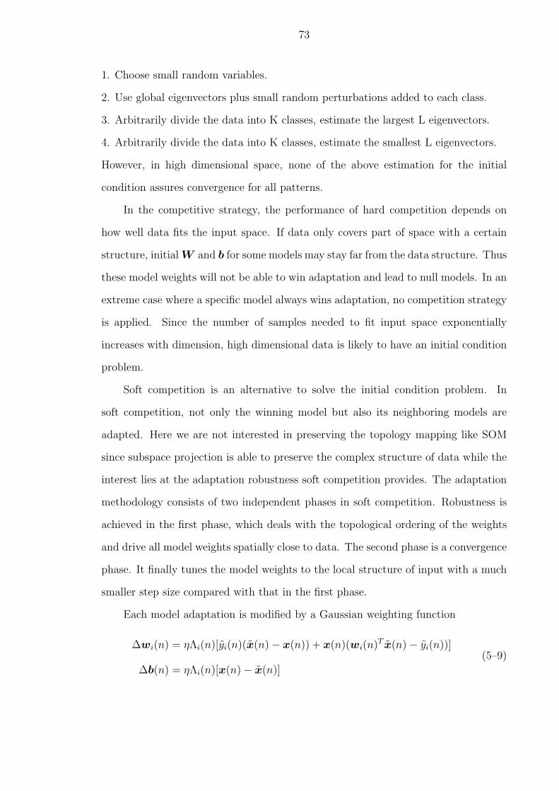
73

1. Choose small random variables.

2. Use global eigenvectors plus small random perturbations added to each class.

3. Arbitrarily divide the data into K classes, estimate the largest L eigenvectors.

4. Arbitrarily divide the data into K classes, estimate the smallest L eigenvectors.

However, in high dimensional space, none of the above estimation for the initial

condition assures convergence for all patterns.

In the competitive strategy, the performance of hard competition depends on

how well data fits the input space. If data only covers part of space with a certain

structure, initial W and b for some models may stay far from the data structure. Thus

these model weights will not be able to win adaptation and lead to null models. In an

extreme case where a specific model always wins adaptation, no competition strategy

is applied. Since the number of samples needed to fit input space exponentially

increases with dimension, high dimensional data is likely to have an initial condition

problem.

Soft competition is an alternative to solve the initial condition problem. In

soft competition, not only the winning model but also its neighboring models are

adapted. Here we are not interested in preserving the topology mapping like SOM

since subspace projection is able to preserve the complex structure of data while the

interest lies at the adaptation robustness soft competition provides. The adaptation

methodology consists of two independent phases in soft competition. Robustness is

achieved in the first phase, which deals with the topological ordering of the weights

and drive all model weights spatially close to data. The second phase is a convergence

phase. It finally tunes the model weights to the local structure of input with a much

smaller step size compared with that in the first phase.

Each model adaptation is modified by a Gaussian weighting function

∆wi(n) = ηΛi(n)[yi(n)(x(n)− x(n)) + x(n)(wi(n)T x(n)− yi(n))]

∆b(n) = ηΛi(n)[x(n)− x(n)]

(5–9)

74

where Λi(n) is the weighting function of the ith model, which has a general form of

Λi(n) = exp(−di(n)2

σ(n)2) (5–10)

where di(n) is a distance measure showing how close the ith model fits the local

cluster and σ(n)2 is the kernel width. In order to derive the proper di(n) and σ(n)2

in competitive subspace projection, a few criterions needs to be satisfied:

1. In each adaptation, the winning model with least MSE should get the largest

adaptation step while the other model adaptations depend on how well they fit the

input.

2. In the first phase of training, the weighting function should be controlled in a

given dynamic range such that all models are robustly adapted independent of data

structure.

3. In the second phase of training, the weighting function should finally approximately

shrink to a delta function centered at the winning model to achieve the final winner-

take-all fashion.

Based on the listed criteria, di(n) and σ(n)2 are such that the weighting function is

given by

Λi(n) = exp(− (ei(n)− ei∗(n))2

1l

∑K−1k=0 f((ek(n)− ei∗(n))2, (ek(n)− ei∗∗(n))2)

) (5–11)

where the reconstruction error in model i, the winning model i∗ and nearest neighbor

to the winning model i∗∗ are ei(n) = xi(n) − x(n), ei∗(n) = xi∗(n) − x(n) and

ei∗∗(n) = xi∗∗(n)−x(n), respectively; f(·) is a nonlinear truncation function to control

the extreme large ei(n) for stable convergence; l represents a scalar proportional to

the epoch index. If i = i∗, Λi(n) = 1 gives the largest step size; otherwise in the

first epoch where k = 1, Λi(n) is always in the range of [0.3679, 1], where assures

the tuning of the neighboring in the first phase of training. In the second phase of

training, a large number of epochs are needed for fine-tuning the input. Thus l will

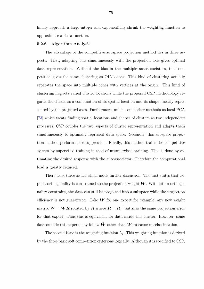
75

finally approach a large integer and exponentially shrink the weighting function to

approximate a delta function.

5.2.6 Algorithm Analysis

The advantage of the competitive subspace projection method lies in three as-

pects. First, adapting bias simultaneously with the projection axis gives optimal

data representation. Without the bias in the multiple autoassociators, the com-

petition gives the same clustering as OIAL does. This kind of clustering actually

separates the space into multiple cones with vertices at the origin. This kind of

clustering neglects varied cluster locations while the proposed CSP methodology re-

gards the cluster as a combination of its spatial location and its shape linearly repre-

sented by the projected axes. Furthermore, unlike some other methods as local PCA

[73] which treats finding spatial locations and shapes of clusters as two independent

processes, CSP couples the two aspects of cluster representation and adapts them

simultaneously to optimally represent data space. Secondly, this subspace projec-

tion method perform noise suppression. Finally, this method trains the competitive

system by supervised training instead of unsupervised training. This is done by es-

timating the desired response with the autoassociator. Therefore the computational

load is greatly reduced.

There exist three issues which needs further discussion. The first states that ex-

plicit orthogonality is constrained to the projection weight W . Without an orthogo-

nality constraint, the data can still be projected into a subspace while the projection

efficiency is not guaranteed. Take W for one expert for example, any new weight

matrix W = WR rotated by R where R = R−1 satisfies the same projection error

for that expert. Thus this is equivalent for data inside this cluster. However, some

data outside this expert may follow W other than W to cause misclassification.

The second issue is the weighting function Λi. This weighting function is derived

by the three basic soft competition criterions logically. Although it is specified to CSP,

76

Λi itself can be generalized to other unsupervised learning problems. It is a comprise

between the softmax activation function in fuzzy clustering and the usually used

Gaussian kernel in self-organizing map (SOM). On one hand, the proposed weighting

function shares the advantage of fuzzy clustering where all the soft competition is

determined by the whole cluster center statistics. This information is more accurate

than the Gaussian kernel in SOM. On the other hand, it incorporates the truncation

nonlinear function into Λi which maintains the flexibility of hard competition as SOM

does after shrinking.

Another issue is the scale ambiguity for inputs. As is known, subspace projection

is independent of the norm while any Euclidean distance clustering methods, e.g.

LBG and K-means, take norm into account. This proposed competitive subspace

projection method is a mixture of projection method and Euclidean distance methods

and thus has scale ambiguity for inputs. A cluster is defined by its local structure,

which means how the local data is grouped. Its center, projection axes and projected

variance are the linear representation of cluster itself which linearly determine the

structure and shape of cluster. Thus, a scalar multiplication can be considered as

a center shift and expanded or shrinking projected variance with the same axes. If

the center is shifted (original center is nonzero), this scalar multiplication should

generate a new cluster while it is arguing if the center is unchanged (original center

is zero). Thus the competitive subspace projection which takes the norm jointly with

the subspace projection is reasonable.

5.2.7 fMRI Application with Competitive Subspace Projection

We are interested in using this proposed method to detect the functional re-

gions in fMRI brain images. The purpose is to detect when and where the response

takes effect inside the brain after stimulus. There are multiple sampling time instants

where each sampling time corresponds to a 2D brain image with the same size. From

another aspect, each pixel in the 2D brain image has its time response, which reflects

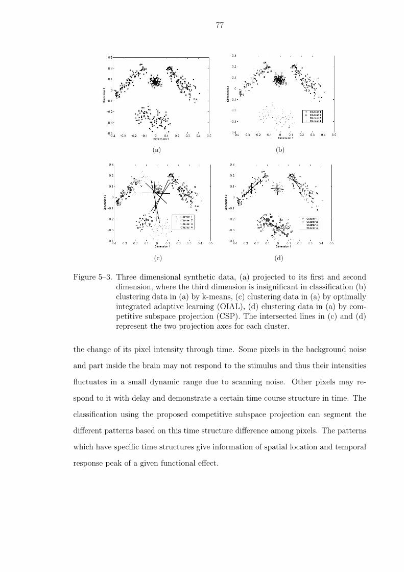
77

(a) (b)

(c) (d)

Figure 5–3. Three dimensional synthetic data, (a) projected to its first and seconddimension, where the third dimension is insignificant in classification (b)clustering data in (a) by k-means, (c) clustering data in (a) by optimallyintegrated adaptive learning (OIAL), (d) clustering data in (a) by com-petitive subspace projection (CSP). The intersected lines in (c) and (d)represent the two projection axes for each cluster.

the change of its pixel intensity through time. Some pixels in the background noise

and part inside the brain may not respond to the stimulus and thus their intensities

fluctuates in a small dynamic range due to scanning noise. Other pixels may re-

spond to it with delay and demonstrate a certain time course structure in time. The

classification using the proposed competitive subspace projection can segment the

different patterns based on this time structure difference among pixels. The patterns

which have specific time structures give information of spatial location and temporal

response peak of a given functional effect.

78

5.3 Results

Clustering Performance Comparison: The synthetic data used to demon-

strate the clustering performance is generated with complex structure. The data

which is three dimensional is projected to its first and second dimensions for classi-

fication since the third dimension is insignificant in segmentation (Fig. 5–3(a)). The

data structure consists of four natural clusters where their shapes are two approxi-

mate rectangles, one circle and one ellipse. The two rectangle clusters approximate

the circle cluster from different directions while the ellipse cluster stays compara-

tively far from the other three. Three clustering methods are compared based on

the synthetic data, which are kmeans, optimally integrated adaptive learning (OIAL)

and competitive subspace projection (CSP). It is shown in Fig. 5–3(b) that kmeans

groups data well except that it misclassifies some samples inside its neighboring end

side of the two rectangle clusters. The reason is that k-means cannot reflect complex

clustering boundary in classification. Fig. 5–3(c) reveals that the segmentation which

OIAL does conforms to separating the input space into multiple cones with the ver-

tex at the origin due to the fact that the in-between cluster centroid distances are

not considered. We can see that CSP gives a reasonable clustering fitting its natural

structure in terms of subspace projection (Fig. 5–3(d)). Here the preserved subspace

dimension is two while the projection axes to the first and second dimensions of the

synthetic input are demonstrated.

Task Detection: The fMRI brain images detecting task–related effects are

collected on eight human volunteers using a 3 Tesla MRI scanner at the UF. A

gradient-echo echo-planar imaging (EPI) pulse sequence was used with the following

scan parameters: TR/TE/FA = 6s/30ms/90o, Field of View = 240mm, matrix size

= 64x64 with an in-plane resolution of 1.875 x 1.875 mm2 and a single slice (3.5 mm

thick). The functional images consist of 750 samples in total.

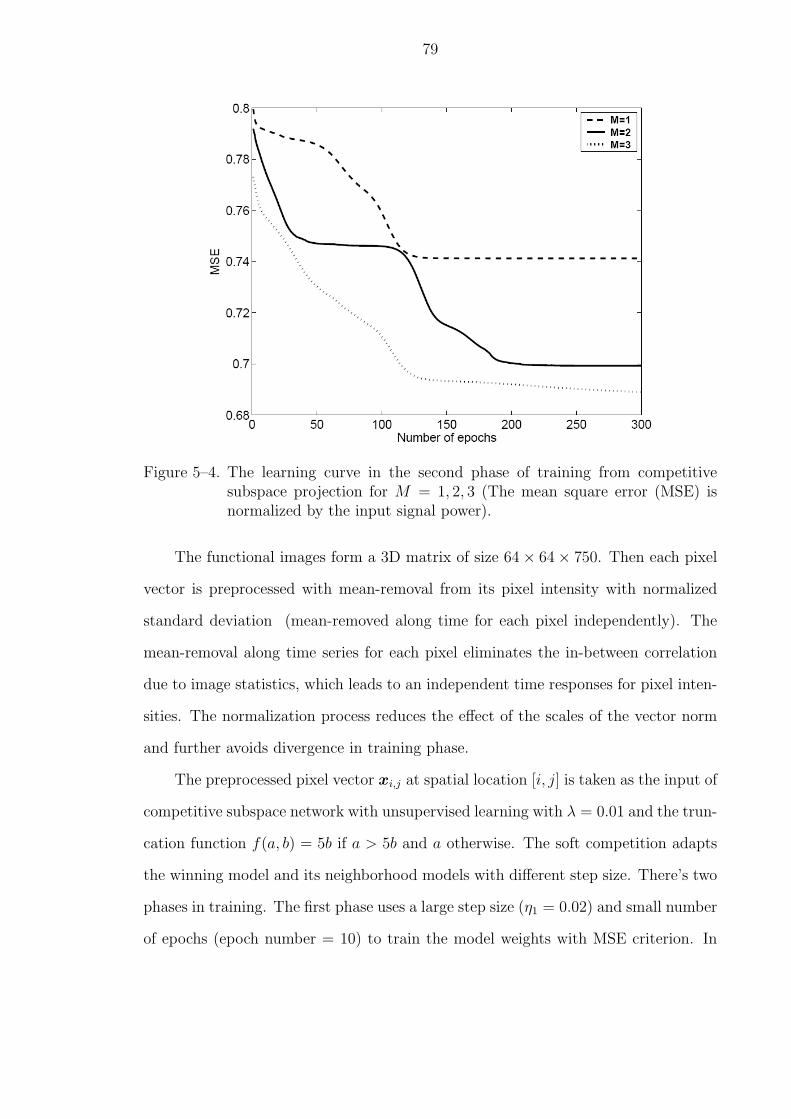
79

Figure 5–4. The learning curve in the second phase of training from competitivesubspace projection for M = 1, 2, 3 (The mean square error (MSE) isnormalized by the input signal power).

The functional images form a 3D matrix of size 64× 64× 750. Then each pixel

vector is preprocessed with mean-removal from its pixel intensity with normalized

standard deviation (mean-removed along time for each pixel independently). The

mean-removal along time series for each pixel eliminates the in-between correlation

due to image statistics, which leads to an independent time responses for pixel inten-

sities. The normalization process reduces the effect of the scales of the vector norm

and further avoids divergence in training phase.

The preprocessed pixel vector xi,j at spatial location [i, j] is taken as the input of

competitive subspace network with unsupervised learning with λ = 0.01 and the trun-

cation function f(a, b) = 5b if a > 5b and a otherwise. The soft competition adapts

the winning model and its neighborhood models with different step size. There’s two

phases in training. The first phase uses a large step size (η1 = 0.02) and small number

of epochs (epoch number = 10) to train the model weights with MSE criterion. In

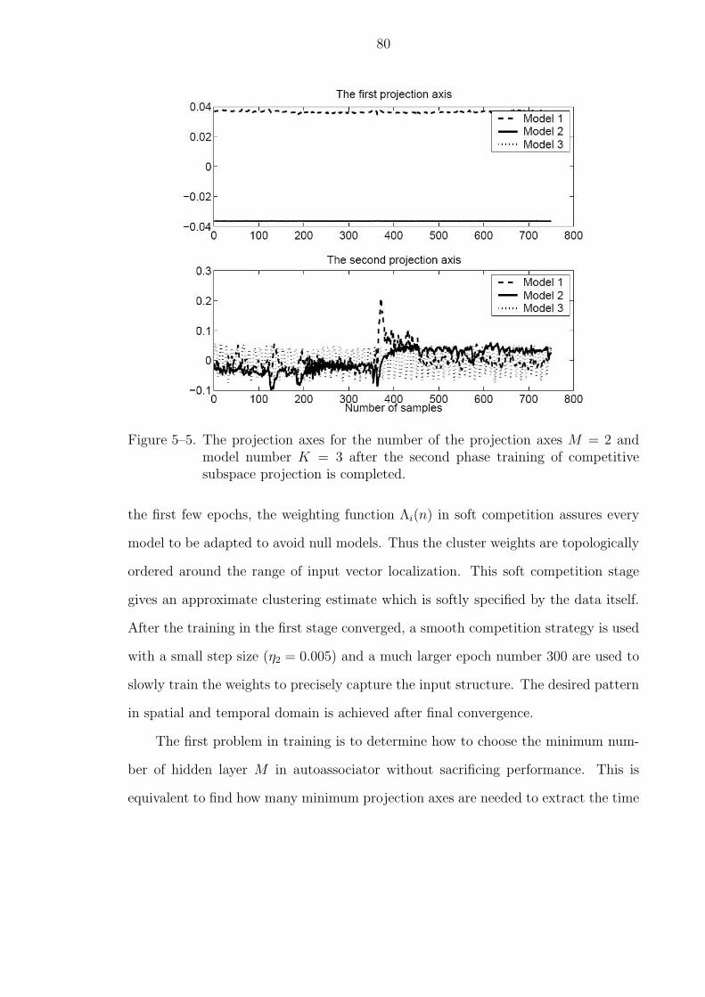
80

Figure 5–5. The projection axes for the number of the projection axes M = 2 andmodel number K = 3 after the second phase training of competitivesubspace projection is completed.

the first few epochs, the weighting function Λi(n) in soft competition assures every

model to be adapted to avoid null models. Thus the cluster weights are topologically

ordered around the range of input vector localization. This soft competition stage

gives an approximate clustering estimate which is softly specified by the data itself.

After the training in the first stage converged, a smooth competition strategy is used

with a small step size (η2 = 0.005) and a much larger epoch number 300 are used to

slowly train the weights to precisely capture the input structure. The desired pattern

in spatial and temporal domain is achieved after final convergence.

The first problem in training is to determine how to choose the minimum num-

ber of hidden layer M in autoassociator without sacrificing performance. This is

equivalent to find how many minimum projection axes are needed to extract the time

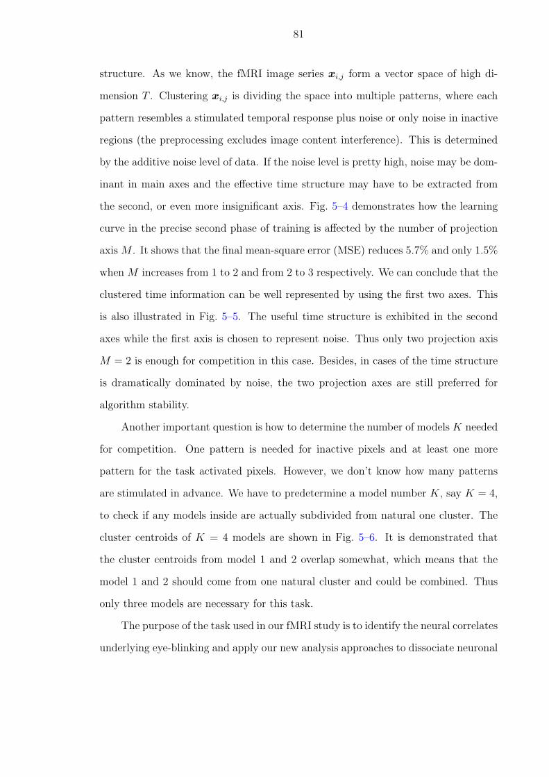
81

structure. As we know, the fMRI image series xi,j form a vector space of high di-

mension T . Clustering xi,j is dividing the space into multiple patterns, where each

pattern resembles a stimulated temporal response plus noise or only noise in inactive

regions (the preprocessing excludes image content interference). This is determined

by the additive noise level of data. If the noise level is pretty high, noise may be dom-

inant in main axes and the effective time structure may have to be extracted from

the second, or even more insignificant axis. Fig. 5–4 demonstrates how the learning

curve in the precise second phase of training is affected by the number of projection

axis M . It shows that the final mean-square error (MSE) reduces 5.7% and only 1.5%

when M increases from 1 to 2 and from 2 to 3 respectively. We can conclude that the

clustered time information can be well represented by using the first two axes. This

is also illustrated in Fig. 5–5. The useful time structure is exhibited in the second

axes while the first axis is chosen to represent noise. Thus only two projection axis

M = 2 is enough for competition in this case. Besides, in cases of the time structure

is dramatically dominated by noise, the two projection axes are still preferred for

algorithm stability.

Another important question is how to determine the number of models K needed

for competition. One pattern is needed for inactive pixels and at least one more

pattern for the task activated pixels. However, we don’t know how many patterns

are stimulated in advance. We have to predetermine a model number K, say K = 4,

to check if any models inside are actually subdivided from natural one cluster. The

cluster centroids of K = 4 models are shown in Fig. 5–6. It is demonstrated that

the cluster centroids from model 1 and 2 overlap somewhat, which means that the

model 1 and 2 should come from one natural cluster and could be combined. Thus

only three models are necessary for this task.

The purpose of the task used in our fMRI study is to identify the neural correlates

underlying eye-blinking and apply our new analysis approaches to dissociate neuronal

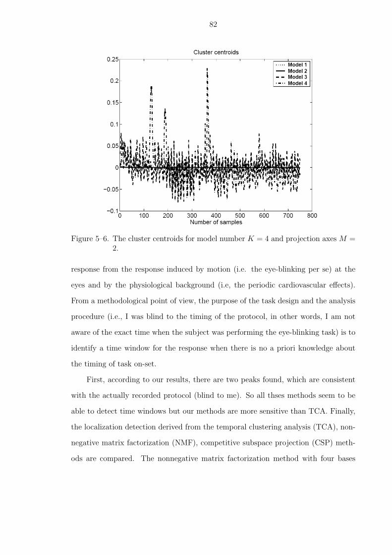
82

Figure 5–6. The cluster centroids for model number K = 4 and projection axes M =2.

response from the response induced by motion (i.e. the eye-blinking per se) at the

eyes and by the physiological background (i.e, the periodic cardiovascular effects).

From a methodological point of view, the purpose of the task design and the analysis

procedure (i.e., I was blind to the timing of the protocol, in other words, I am not

aware of the exact time when the subject was performing the eye-blinking task) is to

identify a time window for the response when there is no a priori knowledge about

the timing of task on-set.

First, according to our results, there are two peaks found, which are consistent

with the actually recorded protocol (blind to me). So all thses methods seem to be

able to detect time windows but our methods are more sensitive than TCA. Finally,

the localization detection derived from the temporal clustering analysis (TCA), non-

negative matrix factorization (NMF), competitive subspace projection (CSP) meth-

ods are compared. The nonnegative matrix factorization method with four bases

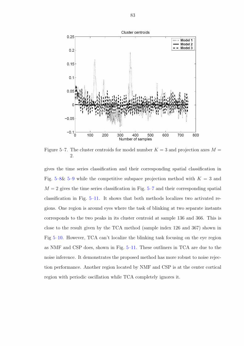
83

Figure 5–7. The cluster centroids for model number K = 3 and projection axes M =2.

gives the time series classification and their corresponding spatial classification in

Fig. 5–8& 5–9 while the competitive subspace projection method with K = 3 and

M = 2 gives the time series classification in Fig. 5–7 and their corresponding spatial

classification in Fig. 5–11. It shows that both methods localizes two activated re-

gions. One region is around eyes where the task of blinking at two separate instants

corresponds to the two peaks in its cluster centroid at sample 136 and 366. This is

close to the result given by the TCA method (sample index 126 and 367) shown in

Fig 5–10. However, TCA can’t localize the blinking task focusing on the eye region

as NMF and CSP does, shown in Fig. 5–11. These outliners in TCA are due to the

noise inference. It demonstrates the proposed method has more robust to noise rejec-

tion performance. Another region located by NMF and CSP is at the center cortical

region with periodic oscillation while TCA completely ignores it.

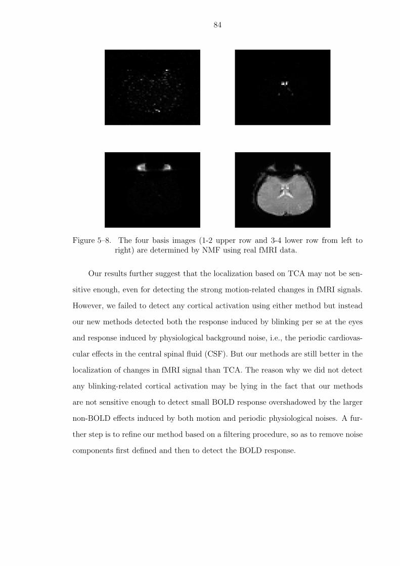
84

Figure 5–8. The four basis images (1-2 upper row and 3-4 lower row from left toright) are determined by NMF using real fMRI data.

Our results further suggest that the localization based on TCA may not be sen-

sitive enough, even for detecting the strong motion-related changes in fMRI signals.

However, we failed to detect any cortical activation using either method but instead

our new methods detected both the response induced by blinking per se at the eyes

and response induced by physiological background noise, i.e., the periodic cardiovas-

cular effects in the central spinal fluid (CSF). But our methods are still better in the

localization of changes in fMRI signal than TCA. The reason why we did not detect

any blinking-related cortical activation may be lying in the fact that our methods

are not sensitive enough to detect small BOLD response overshadowed by the larger

non-BOLD effects induced by both motion and periodic physiological noises. A fur-

ther step is to refine our method based on a filtering procedure, so as to remove noise

components first defined and then to detect the BOLD response.

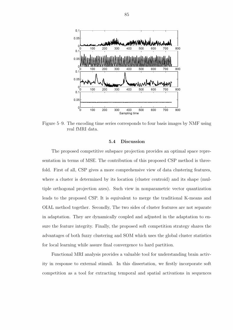
85

Figure 5–9. The encoding time series corresponds to four basis images by NMF usingreal fMRI data.

5.4 Discussion

The proposed competitive subspace projection provides an optimal space repre-

sentation in terms of MSE. The contribution of this proposed CSP method is three-

fold. First of all, CSP gives a more comprehensive view of data clustering features,

where a cluster is determined by its location (cluster centroid) and its shape (mul-

tiple orthogonal projection axes). Such view in nonparametric vector quantization

leads to the proposed CSP. It is equivalent to merge the traditional K-means and

OIAL method together. Secondly, The two sides of cluster features are not separate

in adaptation. They are dynamically coupled and adjusted in the adaptation to en-

sure the feature integrity. Finally, the proposed soft competition strategy shares the

advantages of both fuzzy clustering and SOM which uses the global cluster statistics

for local learning while assure final convergence to hard partition.

Functional MRI analysis provides a valuable tool for understanding brain activ-

ity in response to external stimuli. In this dissertation, we firstly incorporate soft

competition as a tool for extracting temporal and spatial activations in sequences

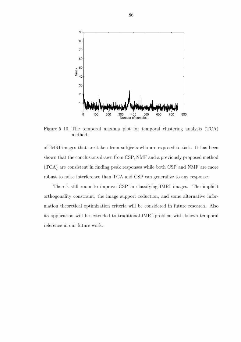
86

Figure 5–10. The temporal maxima plot for temporal clustering analysis (TCA)method.

of fMRI images that are taken from subjects who are exposed to task. It has been

shown that the conclusions drawn from CSP, NMF and a previously proposed method

(TCA) are consistent in finding peak responses while both CSP and NMF are more

robust to noise interference than TCA and CSP can generalize to any response.

There’s still room to improve CSP in classifying fMRI images. The implicit

orthogonality constraint, the image support reduction, and some alternative infor-

mation theoretical optimization criteria will be considered in future research. Also

its application will be extended to traditional fMRI problem with known temporal

reference in our future work.

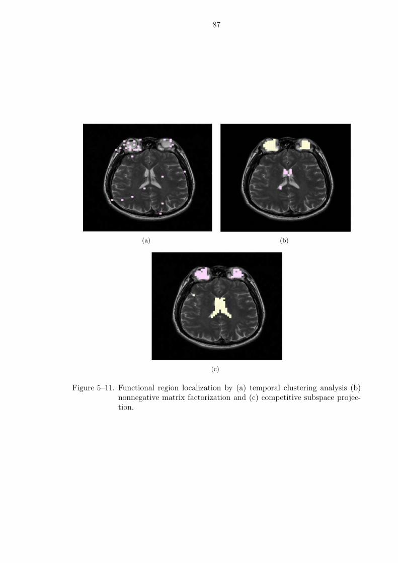
87

(a) (b)

(c)

Figure 5–11. Functional region localization by (a) temporal clustering analysis (b)nonnegative matrix factorization and (c) competitive subspace projec-tion.

CHAPTER 6CONCLUSIONS AND FUTURE WORK

6.1 Conclusions

The sum-of-squares algorithm is a conceptually simple and practical approach in

phased-array MRI that yields the asymptotically optimal SNR in image reconstruc-

tion provided the original coil measurements have high SNR levels. It relies on the

assumption that measurement noise in coil images is spatially WSS. It is proved in

this proposal that this assumption can easily be violated in practical fast collection

MRI. The proposed competitive mixture of local linear experts approach circumvents

this and other possible problems that might influence the SoS reconstruction quality.

The method relies on the local approximation capabilities of the adaptive compet-

itive models, thus its performance can be improved by modifying the local experts

properly (e.g., increasing the input filter-tap size and introducing nonlinearities in the

local experts). Here I investigated the performance of local linear experts combined

linearly and nonlinearly (using an MLP). While the linear combination yielded a 1dB

gain compared to whitened SoS (the best result obtained with the SoS strategy),

the nonlinear combination strategy exhibited its advantage by providing a 5dB SNR

improvement over the whitened SoS, i.e., an additional 4dB SNR gain over the linear

combination. Even if SNR is not a good measure for nonlinear processes, there is

visual improvement between the reconstructed images in Fig. 3–11.

In the proposal, reconstruction results are shown for single snap-shot MRI im-

ages, therefore, the SNR levels and the image quality is poor and insufficient for

practical purposes. However, note that in practice many reconstructed snap-shots

like these are averaged in order to get higher SNR levels. Therefore, the demonstrated

88

89

improvements in the SNR of single snap-shots directly influence two important fac-

tors: 1. the final reconstructed image quality improves assuming the same number

of averaged snap-shots. 2. The image acquisition time is reduced assuming a fixed

SNR so that fewer snap-shots are necessary. However, this measured improvement

in SNR may not extend to less noisy images. There are several issues that need

to be further discussed. The desired response is currently estimated by the average

of the reconstruction from each sample. It may be possible to replace the lengthy

procedure by a single near optimal image with a long scanning time. The relatively

heavy computational load of training needs to be considered despite performance

improvements.

Finally, I would like to address the necessity of the desired response that can

be considered as a shortcoming of this technique. It has been demonstrated that a

system trained in one set of images performs well on another, but it is too early to

quantify the generalization of the technique to any image collected in the same MRI

machine. Effectively I believe that the improved method is extracting the spatial

anisotropy of the coils, but it is doing so by using images that describe the spatial

EM field. Therefore further work is necessarily to quantify these efforts.

6.2 Future Work

Generalization The applicability for the method is predicted in its generaliza-

tion ability. The implicit power of adaptive learning rests on its system identification

capability to extract the system information and store it in the network weights.

This information of the system is estimated from the samples without any statistical

assumption. Then this network can be affiliated to other untrained samples which

implicitly have the same data distribution. Thus we gain the freedom of predicting

unknown data, which has the same metric inherent in nature, with training on a

given amount of samples. The competitive mixture of local linear experts captures

the constant spatial anisotropic coil sensitivities and noise properties from training

90

images directly. How well this competitive local training method learns the inner coil

structure needs to be experimentally validated. Experiments are proposed with three

phantoms representing three different image contents scanned as three training sets

in a given scanning system. Each training trains a completely separate competitive

mixture network. The different three network weights should be approximately con-

stant because they reflect the features of the phased-array coils. If this result holds,

the generalization of the proposed algorithm is validated.

Stability of Competition As stated in the results, there is still a large gap

between the SNR of the averaged image and the output of the local linear experts

which means that there are many possible improvements on the architecture presented

in the dissertation that should be done in future work. First, the adaptation of the

local linear experts should be fine tuned. The issue here in the stability of the

competition over the neighborhoods. As can be seen in Fig. 3–6, the error decreases

very fast in the first few iteration and then fluctuates. This means that the local linear

experts are not being properly adapted probably due to errors in the selection of the

winners. Soft competition may be an alternative. Future work should investigate

how to combine multiple input multiple output models without loosing the sharpness

of the reconstruction, but higher computational complexity can be expected.

Nonlinear Model vs. Linear Model This dissertation proposes a modu-

lar network consisting of local linear models and nonlinear gating. In competition,

multiple linear models are trained from the information of the desired response by

supervised learning, where the desired response is estimated from input. Then the

followed gating network generalizes the linear model outputs given different input

pixels. Each local linear model captures the mapping relationship between the input

and desire, which is assumed to be linear. If the mapping is in general a nonlinear

form, for example the whitened sum-of-squares form which is a second order poly-

nomial, the linear mapping in each local region is only suboptimal. Thus we can

91

consider incorporating the higher order polynomial into the multiple models for bet-

ter function approximations in local regions. However, the training for such multiple

nonlinear models is difficult due to many local minima.

Competitive RBF From a general point of view, each local model is considered

as a kernel which projects data into the specified kernel space. If the kernel space,

which is a functional space, demonstrates a high dimensional space property, nonlin-

ear mapping in input space can be effectively accomplished with linear models. This

sets the basis of radial basis function (RBF) network, where Gaussian basis function

performs the transform from input space to the kernel space and the gating network is

only linear combination. However, the choices of the kernel is normally based on the

input mapping in RBF, for example, Gaussian Mixture Model or K-means algorithm.

It doesn’t absorb any information in clustering from metric between input and desire.

Thus we consider to add a stage of competitive local linear experts to determine the

kernel parameters in RBF. The advantage of this method simplifies the training of

the gating network since it is linear.

Supervised Learning vs. Unsupervised Learning The proposed network

topology is a concatenation of two supervised linear stages. The advantage of the

supervised learning in multiple models lies in learning locally not the input mapping

itself but the input-output metric. However, since during testing the proper com-

bination needs to be found without the desired response, a nonlinear combination

stage is needed for testing data. These combination will usually decrease the perfor-

mance compared only with the outputs of the winner models. This conflict can be

mediated by introducing a competitive unsupervised network in the multiple model

stage instead of a supervised version. The MLP will couple the locality of each au-

toassociative model. Therefore, a local learning strategy instead is more suitable in

combination. The advantage is that only the winning model contribute to the final

92

reconstruction without coupling with the unrelated model outputs. However, the cost

paid is losing the ability to track the local metric between input and desire.

Optimality Analysis From the analysis listed, there exists a large amount of

architectures of modular networks which satisfy the divide-and-conquer strategy. It

may be possible to generalize the network topology by proposing a summarized cost

function, e.g., including L1 penalty. Based on this cost function, we might be able to

analyze the optimality of the multiple model networks under a certain constrains.

Practical Application This dissertation addresses a new adaptive signal process-

ing strategy to MRI parallel image reconstruction. However, this training strategy

has not been utilized in industry for several reasons. First, the training strategy needs

multiple samples for one object to train the system. The multiple real data (taken

from the scanning patients) has two weak points, motion artifacts and training suf-

ficiency. The motion artifact is hard to avoid in sampling due to breath, slight

trembling, etc. The sufficiency of training depends on samples. If the scanned im-

ages are too simple such that inputs only cover a small portion of the whole input

space, the insufficient trained network is not able to generalize to other untrained

images. Besides, the need for multiple conditions corresponding to different scanning

parameters used in the unknown testing complicates the training process. However,

an alternative is to design a training phantom, which doesn’t have any motion arti-

facts. Furthermore, if the phantom is well designed, which means that it has a full

dynamic range for pixel intensities with sharp and smooth boundaries, the training

of the phantom will represent the system well.

Besides, such phantom can be used as a quality measure of the reconstruction

methods. A proposed method is given based on the standard NEMA SNR calculation

as the following. Two near identical testing phantom images are reconstructed and

subtracted toward each other to eliminate any image structure. Then the pure noise

with√

2 standard deviation of one single reconstruction is obtained. Then the local

93

signal power by the local noise power from this subtraction gives the local SNR, which

truly represents the local noise level.

The second reason why the training is not widespread in industry is based on the

current long training time and unguaranteed algorithm robustness due to local min-

ima. What the industry prefers is a direct analytical solution like the sum-of-squares

method. The current development towards chip design for the fast convergence of

training the large amount of image pixels is optimistic. However, the local minima

problem for nonlinear system is still open. We hope to find some asymptotic optimal

and constrained optimal condition for the competitive local linear model in the near

future.

The last reason focuses on improving the image SNR while increasing scanning

time by multiple coils. As we know, the scanning speed can be further improved by

parallel imaging, which undersamples in k-space. This parallel imaging idea can be

further introduced into the adaptive training methodology, where the advantages of

adaptive training is preserved while further improve the imaging speed.

APPENDIX AMRI BIRDCAGE COIL

A transmit only birdcage coil to create an homogeneous excitation profile was

coupled with a 4 channel phased array receiver coil to collect the image data. The

guidance for this construction was provided by David M. Peterson in the RF coil

laboratory at Advanced Magnetic Resonance Imaging and Spectroscopy (ARMIS)

located in the University of Florida’ McKnight Brain Institute. In order to integrate

transmit and receiver coils to the Siemens Allegra MRI system, a custom set of TR

switches and software coil configurations files were implemented.

A 8 pole quadrature birdcage coil was selected to provide a homogeneous transmit

field. Coils are evaluated in the transceive mode and then converted to Tx only by

the addition of decoupling traps that are turned on in the Rx model. The transmit

only birdcage coil with 8 legs is measured using Birdcage Builder v1.0 are shown in

Table. A–1.

Each coil was laid out from pieces of copper strip (3M, Minneapolis, MN) on the

appropriate former. The dimensions for each coil were optimized in order to maximize

the SNR, while preserving the homogeneity of the coils to an acceptable level.

The capacitors (American Technical Ceramics [ATC], 1000V) were then equally

distributed and the resonant mode was verified using a Hewlett Packard (HP) 8752

network analyzer and the near field probe set. Integer multiples of half-wave cables

were made with cable traps, depending upon the desired length.

A cable trap is a narrowband equivalent of wrapping the cable around a ferrite

core. However, since ferrites are not conducive magnetically, these traps are con-

structed from discrete components. The cable is wrapped into an inductive loop, and

a capacitor that is resonant with the shield inductance was placed from one end of

94

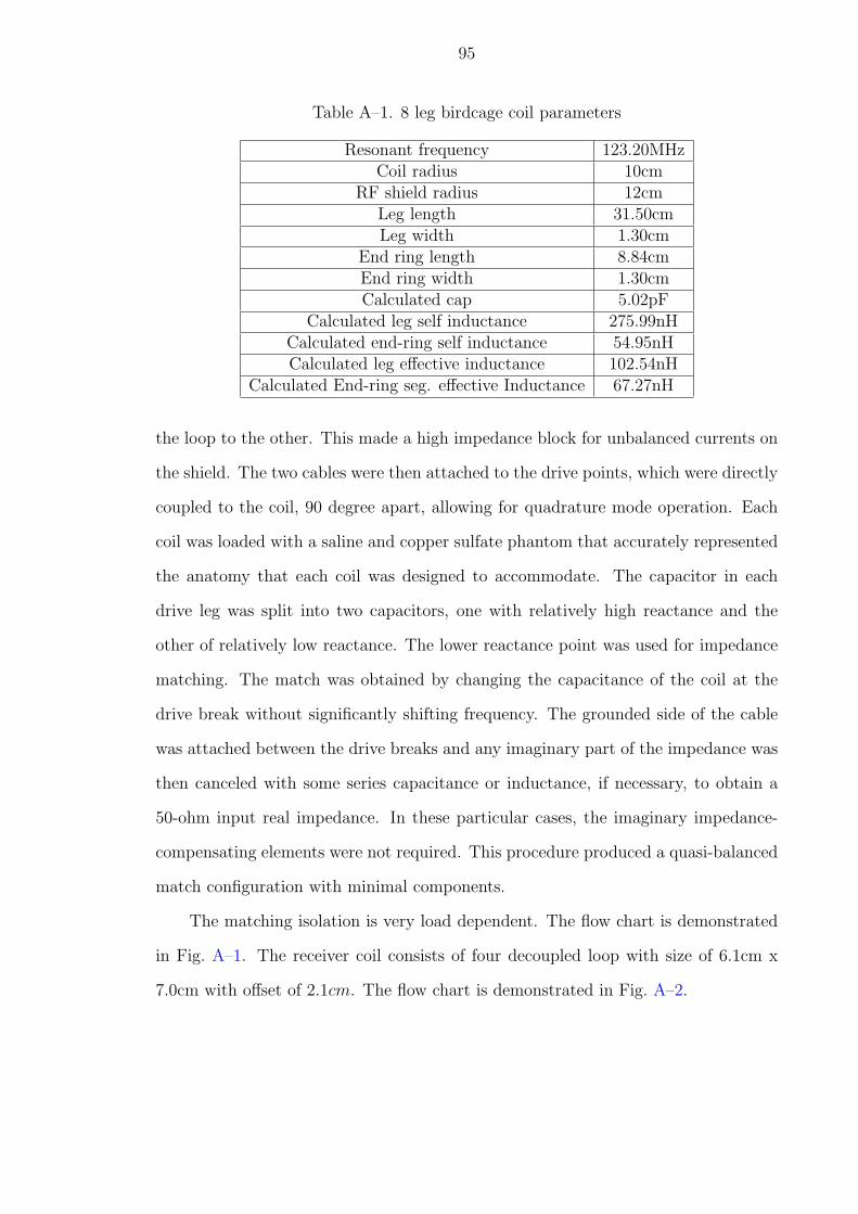
95

Table A–1. 8 leg birdcage coil parameters

Resonant frequency 123.20MHzCoil radius 10cm

RF shield radius 12cmLeg length 31.50cmLeg width 1.30cm

End ring length 8.84cmEnd ring width 1.30cmCalculated cap 5.02pF

Calculated leg self inductance 275.99nHCalculated end-ring self inductance 54.95nHCalculated leg effective inductance 102.54nH

Calculated End-ring seg. effective Inductance 67.27nH

the loop to the other. This made a high impedance block for unbalanced currents on

the shield. The two cables were then attached to the drive points, which were directly

coupled to the coil, 90 degree apart, allowing for quadrature mode operation. Each

coil was loaded with a saline and copper sulfate phantom that accurately represented

the anatomy that each coil was designed to accommodate. The capacitor in each

drive leg was split into two capacitors, one with relatively high reactance and the

other of relatively low reactance. The lower reactance point was used for impedance

matching. The match was obtained by changing the capacitance of the coil at the

drive break without significantly shifting frequency. The grounded side of the cable

was attached between the drive breaks and any imaginary part of the impedance was

then canceled with some series capacitance or inductance, if necessary, to obtain a

50-ohm input real impedance. In these particular cases, the imaginary impedance-

compensating elements were not required. This procedure produced a quasi-balanced

match configuration with minimal components.

The matching isolation is very load dependent. The flow chart is demonstrated

in Fig. A–1. The receiver coil consists of four decoupled loop with size of 6.1cm x

7.0cm with offset of 2.1cm. The flow chart is demonstrated in Fig. A–2.

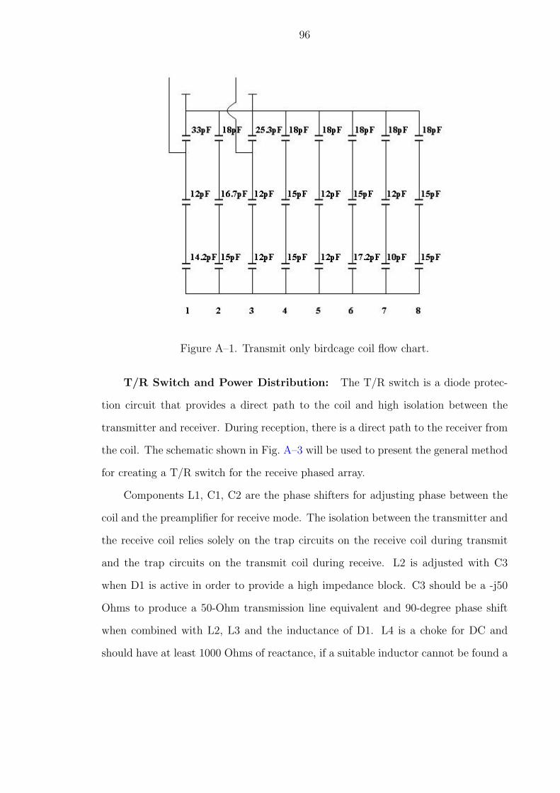
96

Figure A–1. Transmit only birdcage coil flow chart.

T/R Switch and Power Distribution: The T/R switch is a diode protec-

tion circuit that provides a direct path to the coil and high isolation between the

transmitter and receiver. During reception, there is a direct path to the receiver from

the coil. The schematic shown in Fig. A–3 will be used to present the general method

for creating a T/R switch for the receive phased array.

Components L1, C1, C2 are the phase shifters for adjusting phase between the

coil and the preamplifier for receive mode. The isolation between the transmitter and

the receive coil relies solely on the trap circuits on the receive coil during transmit

and the trap circuits on the transmit coil during receive. L2 is adjusted with C3

when D1 is active in order to provide a high impedance block. C3 should be a -j50

Ohms to produce a 50-Ohm transmission line equivalent and 90-degree phase shift

when combined with L2, L3 and the inductance of D1. L4 is a choke for DC and

should have at least 1000 Ohms of reactance, if a suitable inductor cannot be found a

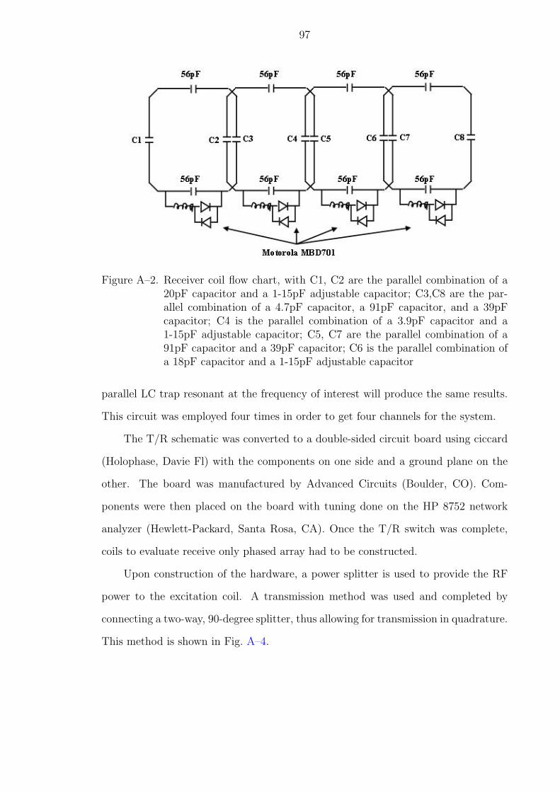
97

Figure A–2. Receiver coil flow chart, with C1, C2 are the parallel combination of a20pF capacitor and a 1-15pF adjustable capacitor; C3,C8 are the par-allel combination of a 4.7pF capacitor, a 91pF capacitor, and a 39pFcapacitor; C4 is the parallel combination of a 3.9pF capacitor and a1-15pF adjustable capacitor; C5, C7 are the parallel combination of a91pF capacitor and a 39pF capacitor; C6 is the parallel combination ofa 18pF capacitor and a 1-15pF adjustable capacitor

parallel LC trap resonant at the frequency of interest will produce the same results.

This circuit was employed four times in order to get four channels for the system.

The T/R schematic was converted to a double-sided circuit board using ciccard

(Holophase, Davie Fl) with the components on one side and a ground plane on the

other. The board was manufactured by Advanced Circuits (Boulder, CO). Com-

ponents were then placed on the board with tuning done on the HP 8752 network

analyzer (Hewlett-Packard, Santa Rosa, CA). Once the T/R switch was complete,

coils to evaluate receive only phased array had to be constructed.

Upon construction of the hardware, a power splitter is used to provide the RF

power to the excitation coil. A transmission method was used and completed by

connecting a two-way, 90-degree splitter, thus allowing for transmission in quadrature.

This method is shown in Fig. A–4.

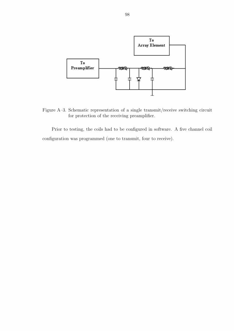
98

Figure A–3. Schematic representation of a single transmit/receive switching circuitfor protection of the receiving preamplifier.

Prior to testing, the coils had to be configured in software. A five channel coil

configuration was programmed (one to transmit, four to receive).

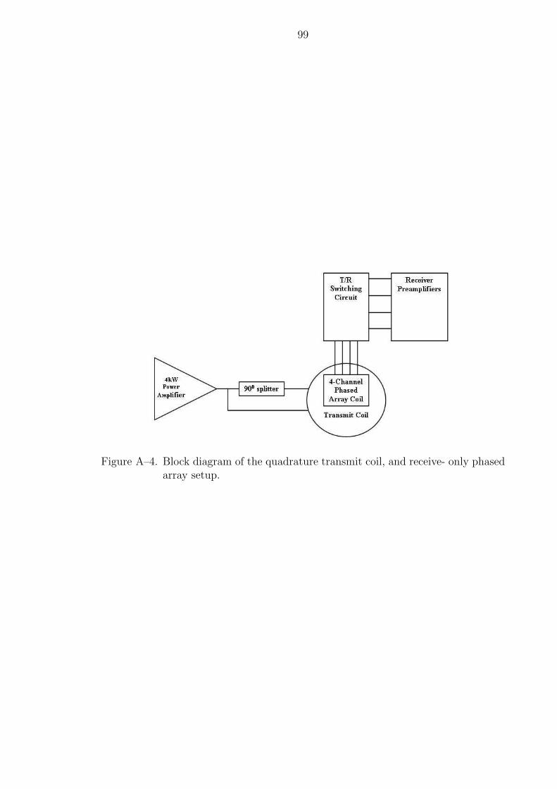
99

Figure A–4. Block diagram of the quadrature transmit coil, and receive- only phasedarray setup.

APPENDIX BMEASURING THE SIGNAL-TO-NOISE RATIO IN MAGNETIC RESONANCE

IMAGING: ACAVEAT

B.1 Introduction

Magnetic resonance imaging (MRI) is a notable medical imaging technique that

has proven to be particularly valuable for examination of the soft tissues in the body

(such as the brain), and it has become an instrumental tool for the diagnosis of stroke

and other significant diseases as well as for pinpointing the focus of diseases such as

epilepsy [21]. It is also considered to be an extremely important instrument for the

study of other parts of the nervous system (such as the spinal cord), as well as various

joints, the thorax, the pelvis and the abdomen. Because of the recent interest in signal

processing for improving the image quality, which is often quantified by the estimated

signal-to-noise ratio (SNR), it is imperative to understand how this measure can be

affected by nonlinear signal processing operations.1

Most MR imaging scenarios are limited by the SNR in the reconstructed image.

In particular, although it is sometimes argued that improving SNR beyond 20 dB are

diagnostically not significant for static imaging (see, e.g., [10, 23, 22]), an improvement

in SNR can always be translated into an increase in acquisition speed and therefore

be used to reduce the imaging cost and motion artifacts. Therefore, improving the

SNR in MR images has become extremely critical for reducing motion artifacts and

in applications where imaging speed is a major concern. Such applications include

1 Although the physical ratio-of-amplitudes is commonly used to quantify SNRin the MRI literature, in this paper, we will assume the engineering convention ofratio-of-powers. There is a square-relationship between the former and the latter.

100

101

imaging of dynamic processes, such as the heart [79]. Also, since an improvement in

SNR can significantly cut imaging times, it can increase the cost-effectiveness of MRI

equipment in a hospital environment as well as decrease breath-holding durations and

other discomforts for patients.

Evaluation of the quality of a real-world image is often a subjective task, and

perhaps due to the absence of more sophisticated indicators, the SNR appears to be

one of the most popularly used measures of the quality of an MR image. In general the

SNR does not measure bias errors (which are often significant), and furthermore there

is not always a clear correlation between the SNR and the image quality as visually

perceived by a human observer, which is more related to the contrast in a broad sense

(see, e.g., [80, Ch. 7] for a discussion of visual image quality). In this communication

we demonstrate that the SNR can be manipulated by nonlinear operations on the

data, and that it is sometimes also difficult to measure objectively. We therefore

believe that caution should be exercised when the SNR is the sole quality measure of

a reconstructed image, or of the improvement offered by a signal processing algorithm,

which possibly employs a nonlinear operation at some stage of processing.

In this study, we assume that a real-valued MR image is already obtained from

the raw k-space data and that necessary corrections to reduce phase distortions may

have been applied as discussed in [81, 82, 83]. However, since the results on the

distortion of SNR under nonlinear operations are true in general, similar effects are

expected to occur if nonlinear techniques are employed when reconstructing images

from the raw k-space data.

B.2 The Signal-to-Noise Ratio (SNR)

As we illustrate in this section, the major drawback of the SNR as a quality mea-

sure is that it is not invariant to nonlinear transformations. Consider an observation

102

model of the form

x = s + e (B–1)

where s is a signal of interest, and e is noise. We assume that both s and e are random

variables. Also, throughout this paper we assume for simplicity that all signals and

noise are real-valued,2 and that the noise is zero-mean3 . The SNR in x is given by:

SNRx =E s2E e2 (B–2)

where E · stands for statistical expectation.

Let us consider the following nonlinear transformation of x:

y = f(x) = f(s + e) = f(s) +∞∑

k=1

f (k)(s)ek

k!(B–3)

where k! is the factorial of k and f (k)(x) is the kth derivative of f(x), assuming that

all derivatives of f(x) are well-defined. The SNR in y is equal to:

SNRy =E f 2(s)

E

(∑∞k=1

f (k)(s)ek

k!

)2

≈ E f 2(s)E ′f 2(s)E e2

(B–4)

where by convention ′f(s) = f (1)(s) and ′f 2(s) = (′f(s))2, and where the approxima-

tion is valid when SNRx À 1. We conclude that SNRy > SNRx exactly when

E f 2(s)E ′f 2(s) > E

s2

(B–5)

2 All results extend to the complex case as well.

3 Note that if magnitude images are considered, the noise is not zero mean, butthe analysis here could be extended to such cases. See, e.g., [84, 81, 85] for morediscussion on the statistics of the noise in MR images.

103

and therefore nonlinear transformations can improve the SNR in a signal, provided

that the function f(x) and the statistical distribution of s are such that (B–5) holds.

In general, the conditions on f(x), under which (B–5) holds, depend on the

distribution of s. However, we can easily study a few special cases. If, for example,

f(x) = x2, then ′f(x) = 2x and hence

SNRy

SNRx

=E f(s)2

E ′f 2(s)E e2 ·E e2E s2 =

E s44(E s2)2 (B–6)

We conclude that SNRy > SNRx if and only if

Es4

> 4

(E

s2

)2 (B–7)

For zero-mean random signals s, (B–7) holds exactly when

κ(s) =E s4 − 3(E s2)2

(E s2)2 > 1 (B–8)

where κ(s) is the Kurtosis of s. (For a Gaussian distribution, κ(s) = 0; distributions

for which κ(s) > 0 are called super-Gaussian, and distributions for which κ(s) < 0

are called sub-Gaussian.) This means that if the probability distribution of the image

is highly super-Gaussian (most natural images are in this class), i.e., denser around

the mean and heavier at the tails (e.g., Laplacian) then the square-operation (such

as the one used in creating magnitude images) could deceivingly demonstrate an

improvement in SNR.

An interesting question is whether it is possible to find a function f(x) such

that SNRy > SNRx regardless of the distribution of s. Without loss of generality,

consider a unit-power signal s (i.e., E s2 = 1). Then from (B–5) SNRy > SNRx

if f 2(s) > ′f 2(s) for all s. This can be achieved if we choose f(s) = as where a

satisfies 1/e < |a| < e, because in that case∣∣ ln |a|

∣∣ < 1 which implies that f 2(s) =

a2s > (ln |a|)2a2s = ′f 2(s). Hence, a nonlinearity in the form of an exponential

function with exponent a in the range 1/e < |a| < e will improve the SNR for any

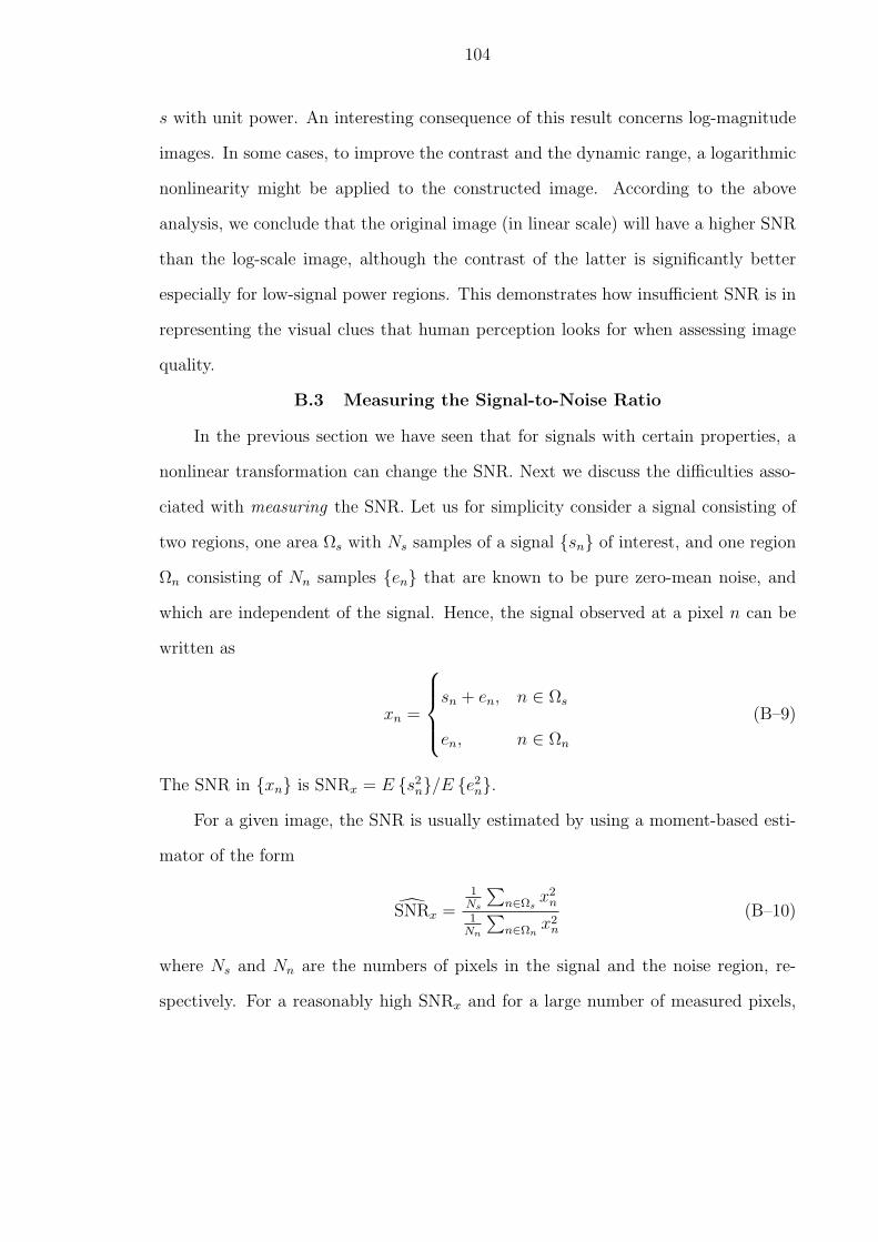
104

s with unit power. An interesting consequence of this result concerns log-magnitude

images. In some cases, to improve the contrast and the dynamic range, a logarithmic

nonlinearity might be applied to the constructed image. According to the above

analysis, we conclude that the original image (in linear scale) will have a higher SNR

than the log-scale image, although the contrast of the latter is significantly better

especially for low-signal power regions. This demonstrates how insufficient SNR is in

representing the visual clues that human perception looks for when assessing image

quality.

B.3 Measuring the Signal-to-Noise Ratio

In the previous section we have seen that for signals with certain properties, a

nonlinear transformation can change the SNR. Next we discuss the difficulties asso-

ciated with measuring the SNR. Let us for simplicity consider a signal consisting of

two regions, one area Ωs with Ns samples of a signal sn of interest, and one region

Ωn consisting of Nn samples en that are known to be pure zero-mean noise, and

which are independent of the signal. Hence, the signal observed at a pixel n can be

written as

xn =

sn + en, n ∈ Ωs

en, n ∈ Ωn

(B–9)

The SNR in xn is SNRx = E s2n/E e2

n.For a given image, the SNR is usually estimated by using a moment-based esti-

mator of the form

SNRx =1

Ns

∑n∈Ωs

x2n

1Nn

∑n∈Ωn

x2n

(B–10)

where Ns and Nn are the numbers of pixels in the signal and the noise region, re-

spectively. For a reasonably high SNRx and for a large number of measured pixels,

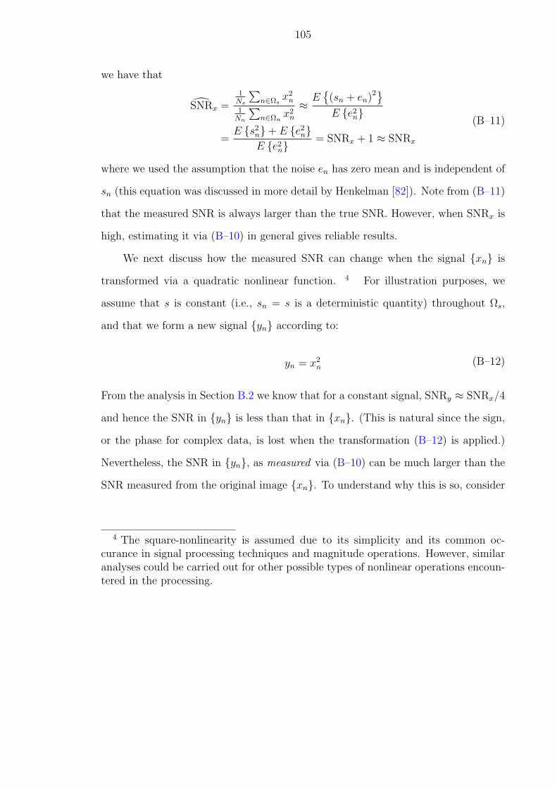
105

we have that

SNRx =1

Ns

∑n∈Ωs

x2n

1Nn

∑n∈Ωn

x2n

≈ E(sn + en)2

E e2n

=E s2

n+ E e2n

E e2n

= SNRx + 1 ≈ SNRx

(B–11)

where we used the assumption that the noise en has zero mean and is independent of

sn (this equation was discussed in more detail by Henkelman [82]). Note from (B–11)

that the measured SNR is always larger than the true SNR. However, when SNRx is

high, estimating it via (B–10) in general gives reliable results.

We next discuss how the measured SNR can change when the signal xn is

transformed via a quadratic nonlinear function. 4 For illustration purposes, we

assume that s is constant (i.e., sn = s is a deterministic quantity) throughout Ωs,

and that we form a new signal yn according to:

yn = x2n

(B–12)

From the analysis in Section B.2 we know that for a constant signal, SNRy ≈ SNRx/4

and hence the SNR in yn is less than that in xn. (This is natural since the sign,

or the phase for complex data, is lost when the transformation (B–12) is applied.)

Nevertheless, the SNR in yn, as measured via (B–10) can be much larger than the

SNR measured from the original image xn. To understand why this is so, consider

4 The square-nonlinearity is assumed due to its simplicity and its common oc-curance in signal processing techniques and magnitude operations. However, similaranalyses could be carried out for other possible types of nonlinear operations encoun-tered in the processing.

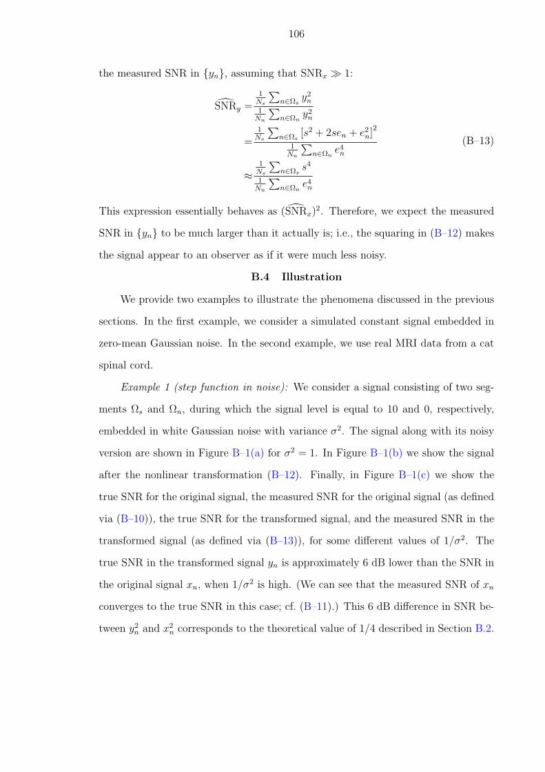
106

the measured SNR in yn, assuming that SNRx À 1:

SNRy =1

Ns

∑n∈Ωs

y2n

1Nn

∑n∈Ωn

y2n

=1

Ns

∑n∈Ωs

[s2 + 2sen + e2n]

2

1Nn

∑n∈Ωn

e4n

≈1

Ns

∑n∈Ωs

s4

1Nn

∑n∈Ωn

e4n

(B–13)

This expression essentially behaves as (SNRx)2. Therefore, we expect the measured

SNR in yn to be much larger than it actually is; i.e., the squaring in (B–12) makes

the signal appear to an observer as if it were much less noisy.

B.4 Illustration

We provide two examples to illustrate the phenomena discussed in the previous

sections. In the first example, we consider a simulated constant signal embedded in

zero-mean Gaussian noise. In the second example, we use real MRI data from a cat

spinal cord.

Example 1 (step function in noise): We consider a signal consisting of two seg-

ments Ωs and Ωn, during which the signal level is equal to 10 and 0, respectively,

embedded in white Gaussian noise with variance σ2. The signal along with its noisy

version are shown in Figure B–1(a) for σ2 = 1. In Figure B–1(b) we show the signal

after the nonlinear transformation (B–12). Finally, in Figure B–1(c) we show the

true SNR for the original signal, the measured SNR for the original signal (as defined

via (B–10)), the true SNR for the transformed signal, and the measured SNR in the

transformed signal (as defined via (B–13)), for some different values of 1/σ2. The

true SNR in the transformed signal yn is approximately 6 dB lower than the SNR in

the original signal xn, when 1/σ2 is high. (We can see that the measured SNR of xn

converges to the true SNR in this case; cf. (B–11).) This 6 dB difference in SNR be-

tween y2n and x2

n corresponds to the theoretical value of 1/4 described in Section B.2.

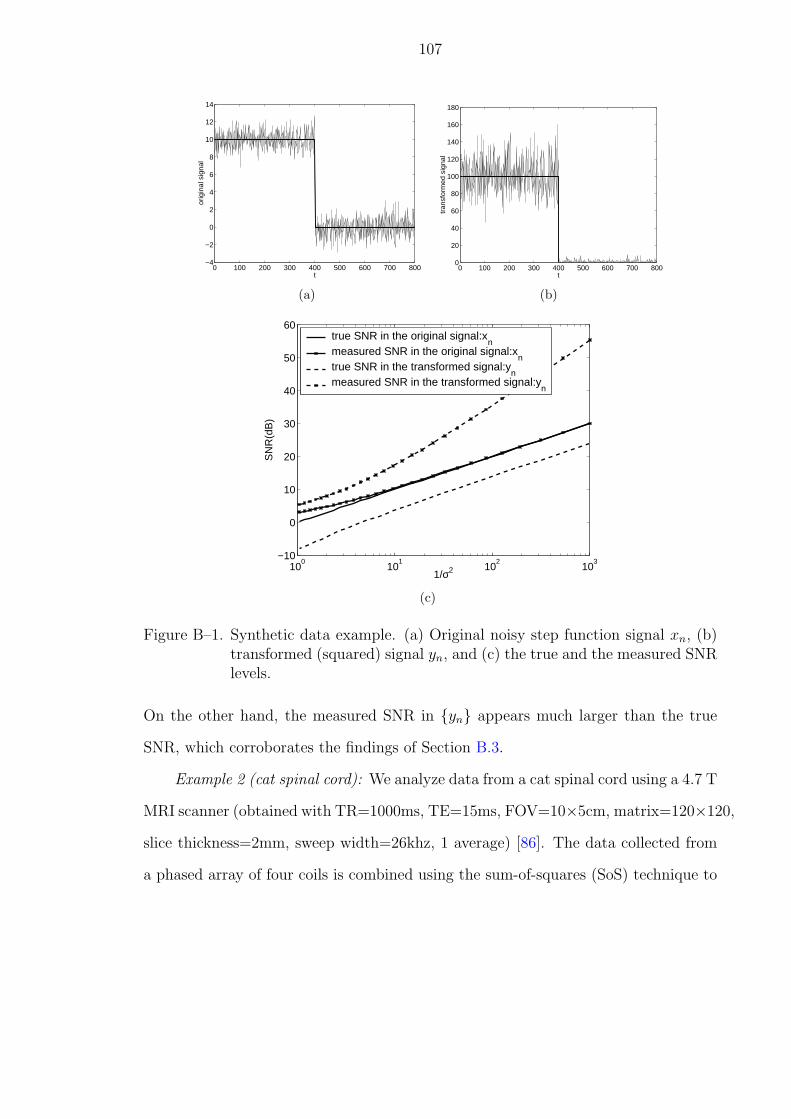
107

0 100 200 300 400 500 600 700 800−4

−2

0

2

4

6

8

10

12

14

t

orig

inal

sig

nal

(a)

0 100 200 300 400 500 600 700 8000

20

40

60

80

100

120

140

160

180

t

tran

sfor

med

sig

nal

(b)

100

101

102

103

−10

0

10

20

30

40

50

60

1/σ2

SN

R(d

B)

true SNR in the original signal:xn

measured SNR in the original signal:xn

true SNR in the transformed signal:yn

measured SNR in the transformed signal:yn

(c)

Figure B–1. Synthetic data example. (a) Original noisy step function signal xn, (b)transformed (squared) signal yn, and (c) the true and the measured SNRlevels.

On the other hand, the measured SNR in yn appears much larger than the true

SNR, which corroborates the findings of Section B.3.

Example 2 (cat spinal cord): We analyze data from a cat spinal cord using a 4.7 T

MRI scanner (obtained with TR=1000ms, TE=15ms, FOV=10×5cm, matrix=120×120,

slice thickness=2mm, sweep width=26khz, 1 average) [86]. The data collected from

a phased array of four coils is combined using the sum-of-squares (SoS) technique to

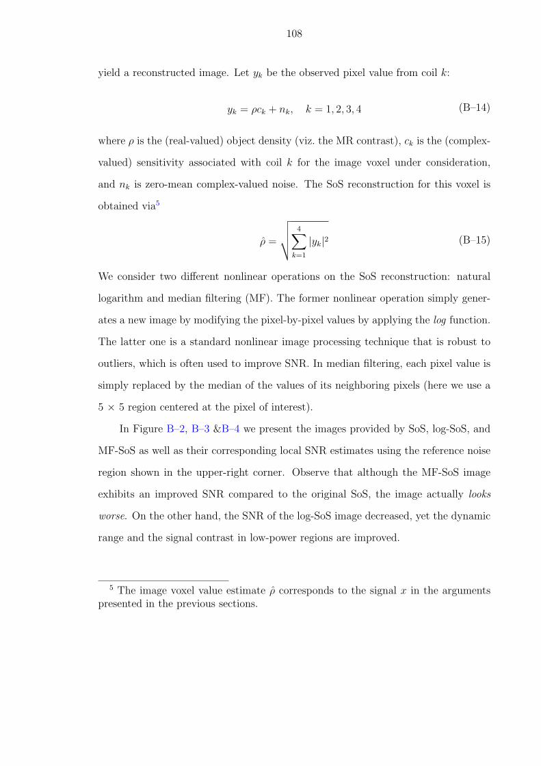
108

yield a reconstructed image. Let yk be the observed pixel value from coil k:

yk = ρck + nk, k = 1, 2, 3, 4 (B–14)

where ρ is the (real-valued) object density (viz. the MR contrast), ck is the (complex-

valued) sensitivity associated with coil k for the image voxel under consideration,

and nk is zero-mean complex-valued noise. The SoS reconstruction for this voxel is

obtained via5

ρ =

√√√√4∑

k=1

|yk|2 (B–15)

We consider two different nonlinear operations on the SoS reconstruction: natural

logarithm and median filtering (MF). The former nonlinear operation simply gener-

ates a new image by modifying the pixel-by-pixel values by applying the log function.

The latter one is a standard nonlinear image processing technique that is robust to

outliers, which is often used to improve SNR. In median filtering, each pixel value is

simply replaced by the median of the values of its neighboring pixels (here we use a

5 × 5 region centered at the pixel of interest).

In Figure B–2, B–3 &B–4 we present the images provided by SoS, log-SoS, and

MF-SoS as well as their corresponding local SNR estimates using the reference noise

region shown in the upper-right corner. Observe that although the MF-SoS image

exhibits an improved SNR compared to the original SoS, the image actually looks

worse. On the other hand, the SNR of the log-SoS image decreased, yet the dynamic

range and the signal contrast in low-power regions are improved.

5 The image voxel value estimate ρ corresponds to the signal x in the argumentspresented in the previous sections.

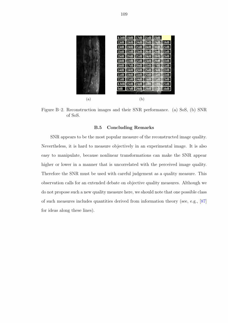
109

(a)

8.3dB 15dB 17dB 21dB 23dB 7.4dB13dB 18dB 24dB 25dB 29dB 18dB13dB 19dB 21dB 24dB 30dB 21dB15dB 22dB 23dB 26dB 29dB 21dB15dB 20dB 21dB 24dB 28dB 23dB18dB 22dB 21dB 23dB 28dB 22dB16dB 17dB 20dB 22dB 27dB 21dB14dB 18dB 23dB 25dB 29dB 22dB11dB 19dB 22dB 25dB 31dB 22dB11dB 21dB 24dB 28dB 31dB 23dB6.9dB 15dB 23dB 30dB 32dB 21dB5dB 17dB 24dB 28dB 32dB 16dB

(b)

Figure B–2. Reconstruction images and their SNR performance. (a) SoS, (b) SNRof SoS.

B.5 Concluding Remarks

SNR appears to be the most popular measure of the reconstructed image quality.

Nevertheless, it is hard to measure objectively in an experimental image. It is also

easy to manipulate, because nonlinear transformations can make the SNR appear

higher or lower in a manner that is uncorrelated with the perceived image quality.

Therefore the SNR must be used with careful judgement as a quality measure. This

observation calls for an extended debate on objective quality measures. Although we

do not propose such a new quality measure here, we should note that one possible class

of such measures includes quantities derived from information theory (see, e.g., [87]

for ideas along these lines).

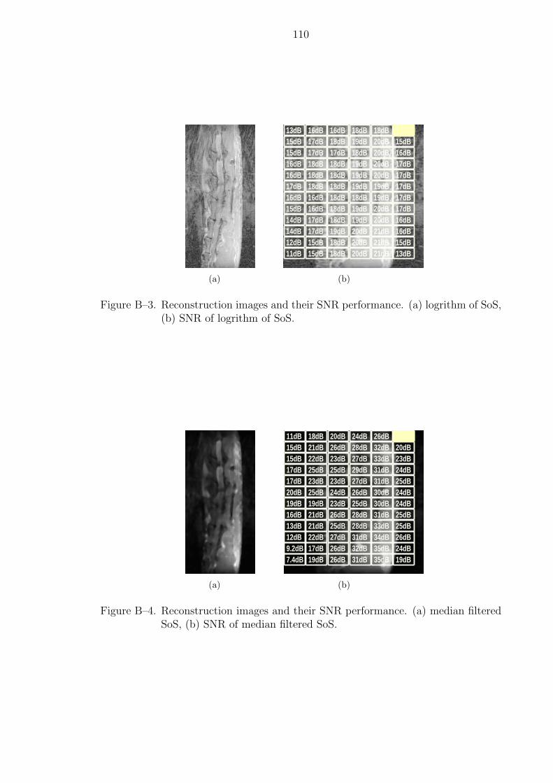
110

(a)

13dB 16dB 16dB 18dB 18dB 12dB15dB 17dB 18dB 19dB 20dB 15dB15dB 17dB 17dB 18dB 20dB 16dB16dB 18dB 18dB 19dB 20dB 17dB16dB 18dB 18dB 19dB 20dB 17dB17dB 18dB 18dB 19dB 19dB 17dB16dB 16dB 18dB 18dB 19dB 17dB15dB 16dB 18dB 19dB 20dB 17dB14dB 17dB 18dB 19dB 20dB 16dB14dB 17dB 19dB 20dB 21dB 16dB12dB 15dB 18dB 20dB 21dB 15dB11dB 15dB 18dB 20dB 21dB 13dB

(b)

Figure B–3. Reconstruction images and their SNR performance. (a) logrithm of SoS,(b) SNR of logrithm of SoS.

(a)

11dB 18dB 20dB 24dB 26dB 9.8dB15dB 21dB 26dB 28dB 32dB 20dB15dB 22dB 23dB 27dB 33dB 23dB17dB 25dB 25dB 29dB 31dB 24dB17dB 23dB 23dB 27dB 31dB 25dB20dB 25dB 24dB 26dB 30dB 24dB19dB 19dB 23dB 25dB 30dB 24dB16dB 21dB 26dB 28dB 31dB 25dB13dB 21dB 25dB 28dB 33dB 25dB12dB 22dB 27dB 31dB 34dB 26dB9.2dB 17dB 26dB 32dB 35dB 24dB7.4dB 19dB 26dB 31dB 35dB 19dB

(b)

Figure B–4. Reconstruction images and their SNR performance. (a) median filteredSoS, (b) SNR of median filtered SoS.

APPENDIX CQUALITY MEASURE FOR RECONSTRUCTION METHODS IN

PHASED-ARRAY MR IMAGES

C.1 Image Quality Measure Review

In general, image quality should an objective measure which extracts the true

object information from images. The goal is to depict well with our own assessment

of equally eye-brain system. The difficulty to find a quantitative measure to images

is due to lack of the knowledge without the visual system as well as noise and blur-

ring effect. Overwhelmingly, signal-to-noise-ratio (SNR), contrast and resolution are

used to describe the image quality. A classification-based image quality measured

is described by the model observer [88]. Hotelling trace criterion (HTO) is used for

the optimal classification of the imaging system [89]. The channelized Hotelling Ob-

server (CHO) provides a good signal detection performance approximating the human

observer [90]. The observer model based quality access roughly estimates how the

two or more object classes are separated by likelihood ratio test. However, it is not

suitable as a quantitative measure to rank medical image quality even with similar

content.

The SNR is considered as a prevalent measure to evaluate the performance of

a magnetic resonance (MR) images. Though it doesn’t provide information for the

image resolution and the image blur, it gives how much noise corrupts the signal

inside the region of interest (ROI). This measure is generally used to estimate intrinsic

physics underlying the magnetic resonance imaging (MRI) scanning system including

the radiofrequency (RF) coil design and the system parameter selection [91, 92]. The

purpose is to find a guideline for a quality measure in MRI by SNR [93].

111

112

In the last decades, multiple phased-array coils are used for fast imaging. The

increased equipment complexity increases the SNR while equivalently reduce the scan-

ning time which has the benefits of reducing the motion artifacts of the image. The

sum-of-squares (SoS) method, proposed by Roemer et al. [10], sets the foundation

of phased-array image reconstruction and it is prevalent in the industry. Based on

SoS, a substantial body of reconstruction methods have been proposed to reconstruct

coil images. However, no efforts has been reported on the comparison among how to

effectively evaluate the reconstruction performance by a proper SNR measure. The

difficulties lie in two aspects. On one hand, the reconstruction is implicitly nonlin-

ear. Any nonlinear transform can unlimitedly increase the SNR estimated by a single

acquisition image sample without affecting the true signal performance in ROI [94].

Thus a fair evaluation how the nonlinear transform affects the image quality inside

ROI needs to be studied. On the other hand, though the noise properties are well

studied in [95], the noise statistics after the nonlinear transform can be arbitrarily

anything, where no parametric estimation can be used here. In this paper, we study

the reconstructed image quality problem and incorporate a non-parametric noise sta-

tistics measure into the SNR.

C.2 Methods

C.2.1 Traditional SNR measures

Two main SNR techniques are calculated based on a single or a dual image

acquisition [96]. For a single image acquisition, the SNR SNRsingle is computed as

SNRsingle = 0.655Ms

SDb

(C–1)

where Ms is the average square root of signal power in ROI, SDb is the ensemble

standard deviation of the noise selected in the background region. The background

0.655 factor is due to the skewed noise distribution based on the magnitude im-

age from the Fourier transform [97]. This fashion of SNR calculation is consistent,

113

where no scanner stability needs to be considered, such that no image registration

is required. However, it has the disadvantage that artefacts from ghost images and

non-uniformities can be projected into the background areas. Besides, it is hard to

validate the noise power in the background area is equivalent to that in the signal

region based on this SNR measurement.

Another way to calculate SNR is according to the dual acquisition

SNRdual =√

2Ms1

SD1−2(C–2)

where Ms1 is the average square root of signal power in ROI on the first image, SD1−2

is the ensemble standard deviation in the ROI on the subtraction image. It has the

opposite advantage and disadvantage compared with the single acquisition.

C.2.2 Local nonparametric SNR measure

The proposed Local nonparametric SNR measure is also based on a dual image

collection, assuming the only difference between images is noise. 1 Since the image

content in ROI may represent varied SNR properties, a global SNR measure is not

sufficient. The ROI can be divided into subregions, let’s say 20× 20 squares, SNR is

calculated in seach subregion

SNRdual,k =√

2Ms1,k

SD1−2,k

(C–3)

where i, j is the kth subregion and M and SD denote the nonparametric estimates of

the square root of signal power and noise power. Since the signal and noise on the

reconstructed image already pass through a nonlinear system, their probability den-

sity function (pdf) can not be uniform distributed. Thus their first order and second

1 This can be achieved by scanning phantom assuming the stability of the scanningsystem; otherwise image registration and motion artefacts cancellation is needed forscanning patients.

114

order statistics can not be estimated as an ensemble average. However, nonparamet-

ric Parzen window provides a way to estimate pdf from data samples. Therefore, the

noise power SD1−2,i,j can be estimated using Parzen window as

SD1−2,k =

√∫(∆xk − µ∆xk

)2f(∆xk)dxk

=

√√√√ 1

Nk

Nk∑j=1

∆x2j

Nk∑i=1

G(∆xj −∆xi, σ2k)− (

1

Nk

Nk∑j=1

∆xj

Nk∑i=1

G(∆xj −∆xi, σ2k))

2

(C–4)

where ∆xk is the subtraction data sample and Nk is total number of samples in the

kth subregion, f(xk) is the pdf of xk, G(·) is the Gaussian kernel used to smooth the

pdf estimation with kernel width σ2k. Then the square root of signal power Ms1,k is

estimated as

Mx1,k =

√∫x12

kf(x1k)dx1k − 2SD21−2,k

=

√√√√ 1

Nk

Nk∑j=1

x12j

Nk∑i=1

G(x1j − x1i, σ2k)− 2SD2

1−2,k

(C–5)

where x1k is the data sample in the kth subregion from the first image.

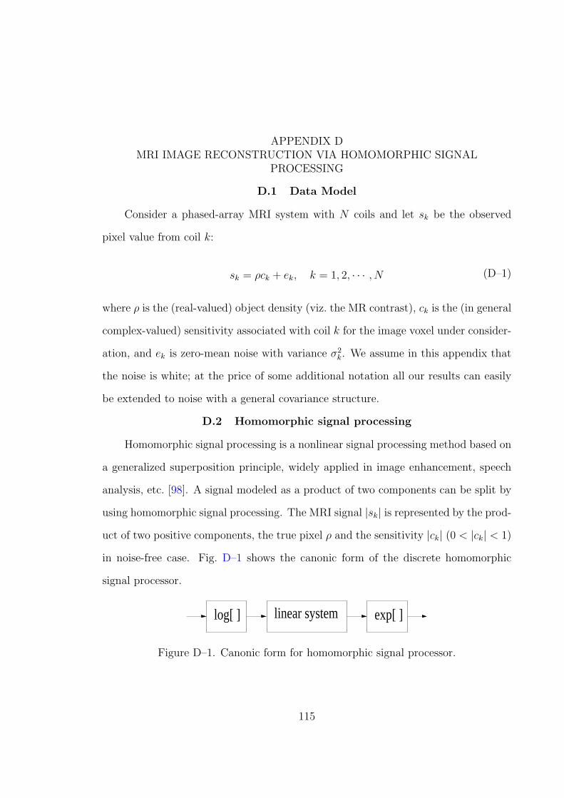
APPENDIX DMRI IMAGE RECONSTRUCTION VIA HOMOMORPHIC SIGNAL

PROCESSING

D.1 Data Model

Consider a phased-array MRI system with N coils and let sk be the observed

pixel value from coil k:

sk = ρck + ek, k = 1, 2, · · · , N (D–1)

where ρ is the (real-valued) object density (viz. the MR contrast), ck is the (in general

complex-valued) sensitivity associated with coil k for the image voxel under consider-

ation, and ek is zero-mean noise with variance σ2k. We assume in this appendix that

the noise is white; at the price of some additional notation all our results can easily

be extended to noise with a general covariance structure.

D.2 Homomorphic signal processing

Homomorphic signal processing is a nonlinear signal processing method based on

a generalized superposition principle, widely applied in image enhancement, speech

analysis, etc. [98]. A signal modeled as a product of two components can be split by

using homomorphic signal processing. The MRI signal |sk| is represented by the prod-

uct of two positive components, the true pixel ρ and the sensitivity |ck| (0 < |ck| < 1)

in noise-free case. Fig. D–1 shows the canonic form of the discrete homomorphic

signal processor.

linear systemlog[ ] exp[ ]

Figure D–1. Canonic form for homomorphic signal processor.

115

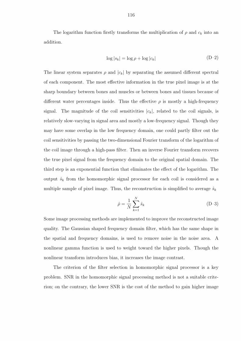
116

The logarithm function firstly transforms the multiplication of ρ and ck into an

addition.

log |sk| = log ρ + log |ck| (D–2)

The linear system separates ρ and |ck| by separating the assumed different spectral

of each component. The most effective information in the true pixel image is at the

sharp boundary between bones and muscles or between bones and tissues because of

different water percentages inside. Thus the effective ρ is mostly a high-frequency

signal. The magnitude of the coil sensitivities |ck|, related to the coil signals, is

relatively slow-varying in signal area and mostly a low-frequency signal. Though they

may have some overlap in the low frequency domain, one could partly filter out the

coil sensitivities by passing the two-dimensional Fourier transform of the logarithm of

the coil image through a high-pass filter. Then an inverse Fourier transform recovers

the true pixel signal from the frequency domain to the original spatial domain. The

third step is an exponential function that eliminates the effect of the logarithm. The

output sk from the homomorphic signal processor for each coil is considered as a

multiple sample of pixel image. Thus, the reconstruction is simplified to average sk

ρ =1

N

N∑

k=1

sk (D–3)

Some image processing methods are implemented to improve the reconstructed image

quality. The Gaussian shaped frequency domain filter, which has the same shape in

the spatial and frequency domains, is used to remove noise in the noise area. A

nonlinear gamma function is used to weight toward the higher pixels. Though the

nonlinear transform introduces bias, it increases the image contrast.

The criterion of the filter selection in homomorphic signal processor is a key

problem. SNR in the homomorphic signal processing method is not a suitable crite-

rion; on the contrary, the lower SNR is the cost of the method to gain higher image

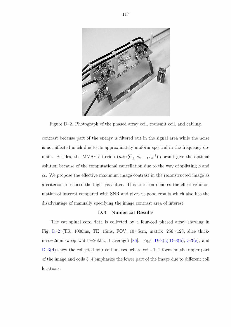
117

Figure D–2. Photograph of the phased array coil, transmit coil, and cabling.

contrast because part of the energy is filtered out in the signal area while the noise

is not affected much due to its approximately uniform spectral in the frequency do-

main. Besides, the MMSE criterion (min∑

k |sk − ρck|2) doesn’t give the optimal

solution because of the computational cancellation due to the way of splitting ρ and

ck. We propose the effective maximum image contrast in the reconstructed image as

a criterion to choose the high-pass filter. This criterion denotes the effective infor-

mation of interest compared with SNR and gives us good results which also has the

disadvantage of manually specifying the image contrast area of interest.

D.3 Numerical Results

The cat spinal cord data is collected by a four-coil phased array showing in

Fig. D–2 (TR=1000ms, TE=15ms, FOV=10×5cm, matrix=256×128, slice thick-

ness=2mm,sweep width=26khz, 1 average) [86]. Figs. D–3(a),D–3(b),D–3(c), and

D–3(d) show the collected four coil images, where coils 1, 2 focus on the upper part

of the image and coils 3, 4 emphasize the lower part of the image due to different coil

locations.

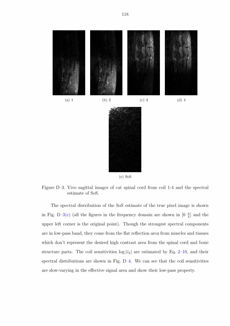
118

(a) 1 (b) 2 (c) 3 (d) 4

(e) SoS

Figure D–3. Vivo sagittal images of cat spinal cord from coil 1-4 and the spectralestimate of SoS.

The spectral distribution of the SoS estimate of the true pixel image is shown

in Fig. D–3(e) (all the figures in the frequency domain are shown in [0 π4] and the

upper left corner is the original point). Though the strongest spectral components

are in low-pass band, they come from the flat reflection area from muscles and tissues

which don’t represent the desired high contrast area from the spinal cord and bone

structure parts. The coil sensitivities log |ck| are estimated by Eq. 2–10, and their

spectral distributions are shown in Fig. D–4. We can see that the coil sensitivities

are slow-varying in the effective signal area and show their low-pass property.

119

(a) Coil 1 (b) Coil 2 (c) Coil 3 (d) Coil 4

(e) Coil 1 (f) Coil 2 (g) Coil 3 (h) Coil 4

Figure D–4. (Upper row) Spatial distribution of the coil sensitivities for four coilsignals. (Lower row) Spectral distribution of the coil sensitivities forfour coil signals.

Thus a high-pass filter is designed to filter the coil sensitivities. The cutoff fre-

quency and the stopband magnitude of the filter are chosen based on the effective

maximum image contrast criterion (the filter order adjustment is not considered for

simplicity). Fig. D–5 shows that the image contrast surface has a global maximum

and the magnitude at the peak is over two times higher than that in SoS. Based on

the filter with peak contrast in Fig. D–6, the true pixel image is reconstructed by

the filter outputs for each coil. The proposed method demonstrates visually better

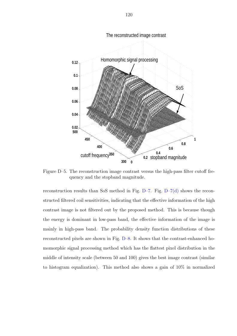
120

00.2

0.40.6

0.81

300

350

400

450

5000.02

0.04

0.06

0.08

0.1

0.12

stopband magnitude

The reconstructed image contrast

cutoff frequency

SoS

Homomorphic signal processing

Figure D–5. The reconstruction image contrast versus the high-pass filter cutoff fre-quency and the stopband magnitude.

reconstruction results than SoS method in Fig. D–7. Fig. D–7(d) shows the recon-

structed filtered coil sensitivities, indicating that the effective information of the high

contrast image is not filtered out by the proposed method. This is because though

the energy is dominant in low-pass band, the effective information of the image is

mainly in high-pass band. The probability density function distributions of these

reconstructed pixels are shown in Fig. D–8. It shows that the contrast-enhanced ho-

momorphic signal processing method which has the flattest pixel distribution in the

middle of intensity scale (between 50 and 100) gives the best image contrast (similar

to histogram equalization). This method also shows a gain of 10% in normalized

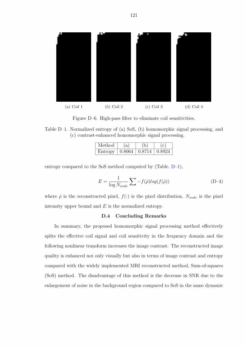
121

(a) Coil 1 (b) Coil 2 (c) Coil 3 (d) Coil 4

Figure D–6. High-pass filter to eliminate coil sensitivities.

Table D–1. Normalized entropy of (a) SoS, (b) homomorphic signal processing, and(c) contrast-enhanced homomorphic signal processing.

Method (a) (b) (c)Entropy 0.8064 0.8714 0.8924

entropy compared to the SoS method computed by (Table. D–1),

E =1

log Nscale

∑−f(ρ)log(f(ρ)) (D–4)

where ρ is the reconstructed pixel, f(·) is the pixel distribution, Nscale is the pixel

intensity upper bound and E is the normalized entropy.

D.4 Concluding Remarks

In summary, the proposed homomorphic signal processing method effectively

splits the effective coil signal and coil sensitivity in the frequency domain and the

following nonlinear transform increases the image contrast. The reconstructed image

quality is enhanced not only visually but also in terms of image contrast and entropy

compared with the widely implemented MRI reconstructed method, Sum-of-squares

(SoS) method. The disadvantage of this method is the decrease in SNR due to the

enlargement of noise in the background region compared to SoS in the same dynamic

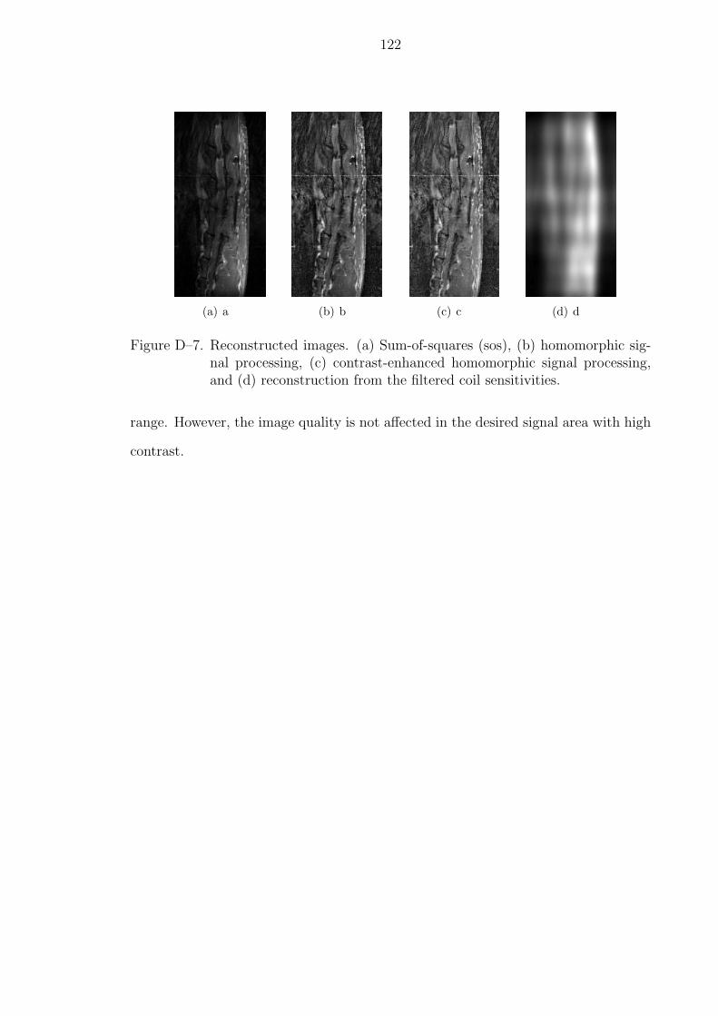
122

(a) a (b) b (c) c (d) d

Figure D–7. Reconstructed images. (a) Sum-of-squares (sos), (b) homomorphic sig-nal processing, (c) contrast-enhanced homomorphic signal processing,and (d) reconstruction from the filtered coil sensitivities.

range. However, the image quality is not affected in the desired signal area with high

contrast.

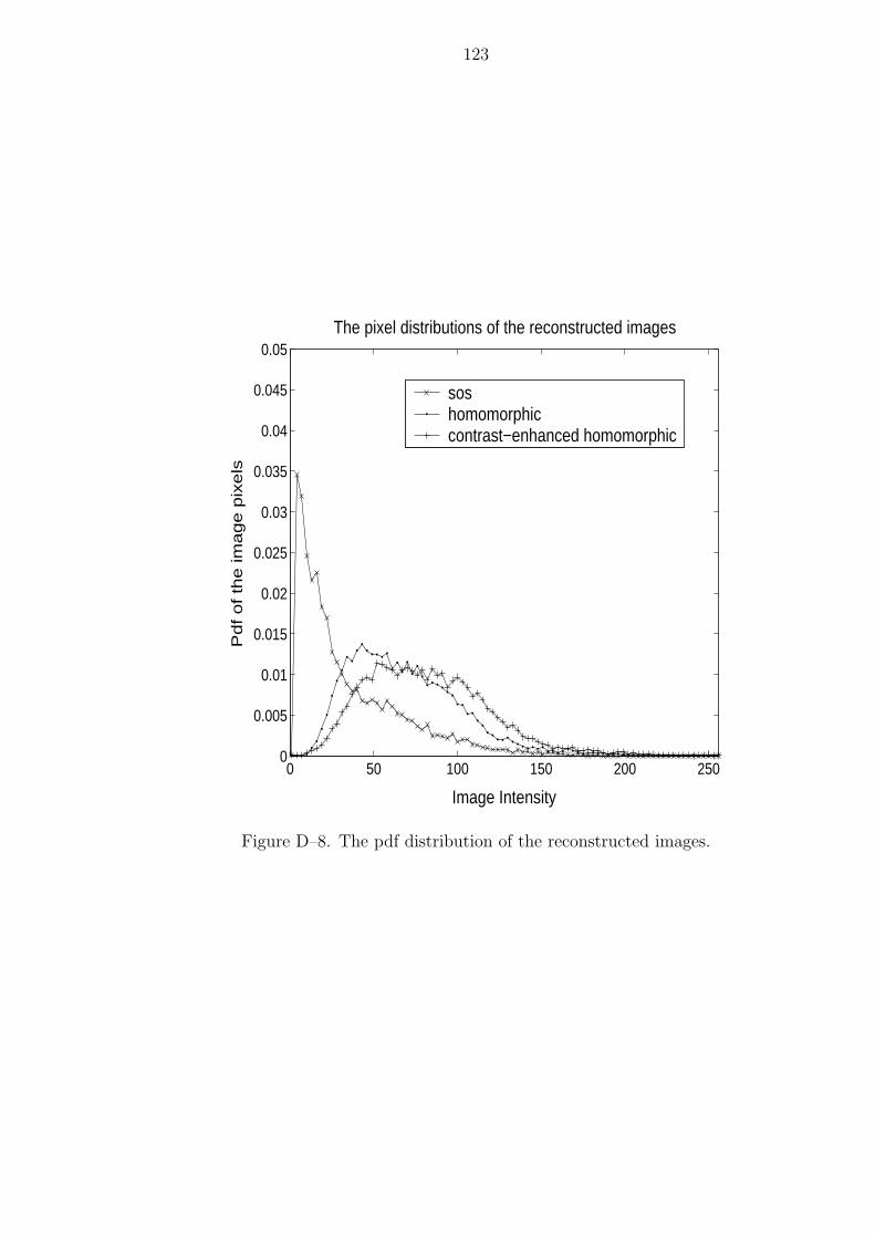
123

0 50 100 150 200 2500

0.005

0.01

0.015

0.02

0.025

0.03

0.035

0.04

0.045

0.05The pixel distributions of the reconstructed images

Image Intensity

Pd

f o

f th

e im

ag

e p

ixe

ls

soshomomorphiccontrast−enhanced homomorphic

Figure D–8. The pdf distribution of the reconstructed images.

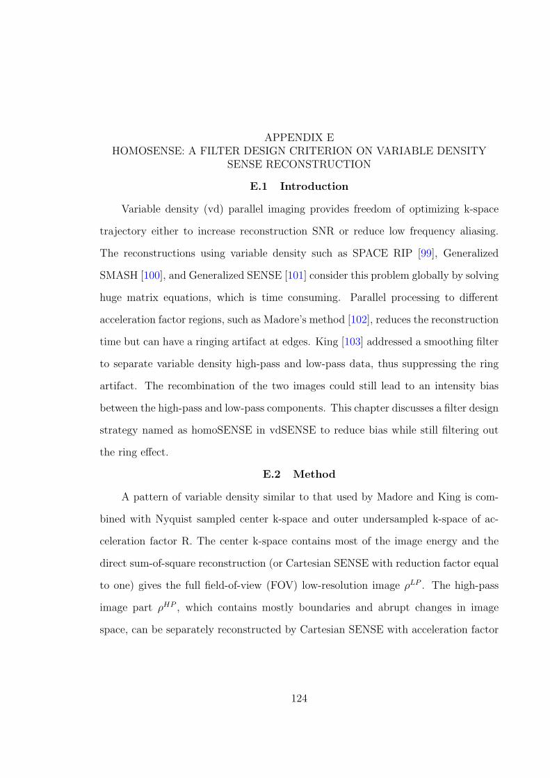
APPENDIX EHOMOSENSE: A FILTER DESIGN CRITERION ON VARIABLE DENSITY

SENSE RECONSTRUCTION

E.1 Introduction

Variable density (vd) parallel imaging provides freedom of optimizing k-space

trajectory either to increase reconstruction SNR or reduce low frequency aliasing.

The reconstructions using variable density such as SPACE RIP [99], Generalized

SMASH [100], and Generalized SENSE [101] consider this problem globally by solving

huge matrix equations, which is time consuming. Parallel processing to different

acceleration factor regions, such as Madore’s method [102], reduces the reconstruction

time but can have a ringing artifact at edges. King [103] addressed a smoothing filter

to separate variable density high-pass and low-pass data, thus suppressing the ring

artifact. The recombination of the two images could still lead to an intensity bias

between the high-pass and low-pass components. This chapter discusses a filter design

strategy named as homoSENSE in vdSENSE to reduce bias while still filtering out

the ring effect.

E.2 Method

A pattern of variable density similar to that used by Madore and King is com-

bined with Nyquist sampled center k-space and outer undersampled k-space of ac-

celeration factor R. The center k-space contains most of the image energy and the

direct sum-of-square reconstruction (or Cartesian SENSE with reduction factor equal

to one) gives the full field-of-view (FOV) low-resolution image ρLP . The high-pass

image part ρHP , which contains mostly boundaries and abrupt changes in image

space, can be separately reconstructed by Cartesian SENSE with acceleration factor

124

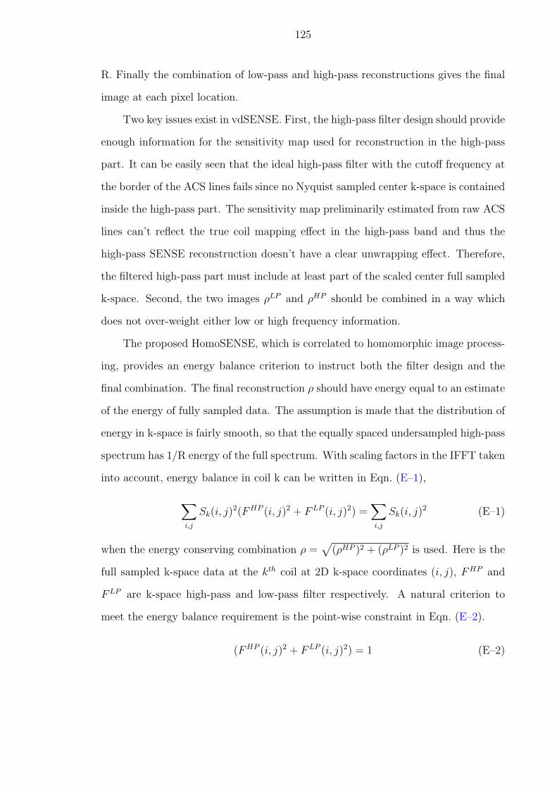
125

R. Finally the combination of low-pass and high-pass reconstructions gives the final

image at each pixel location.

Two key issues exist in vdSENSE. First, the high-pass filter design should provide

enough information for the sensitivity map used for reconstruction in the high-pass

part. It can be easily seen that the ideal high-pass filter with the cutoff frequency at

the border of the ACS lines fails since no Nyquist sampled center k-space is contained

inside the high-pass part. The sensitivity map preliminarily estimated from raw ACS

lines can’t reflect the true coil mapping effect in the high-pass band and thus the

high-pass SENSE reconstruction doesn’t have a clear unwrapping effect. Therefore,

the filtered high-pass part must include at least part of the scaled center full sampled

k-space. Second, the two images ρLP and ρHP should be combined in a way which

does not over-weight either low or high frequency information.

The proposed HomoSENSE, which is correlated to homomorphic image process-

ing, provides an energy balance criterion to instruct both the filter design and the

final combination. The final reconstruction ρ should have energy equal to an estimate

of the energy of fully sampled data. The assumption is made that the distribution of

energy in k-space is fairly smooth, so that the equally spaced undersampled high-pass

spectrum has 1/R energy of the full spectrum. With scaling factors in the IFFT taken

into account, energy balance in coil k can be written in Eqn. (E–1),

∑i,j

Sk(i, j)2(FHP (i, j)2 + FLP (i, j)2) =

∑i,j

Sk(i, j)2 (E–1)

when the energy conserving combination ρ =√

(ρHP )2 + (ρLP )2 is used. Here is the

full sampled k-space data at the kth coil at 2D k-space coordinates (i, j), FHP and

FLP are k-space high-pass and low-pass filter respectively. A natural criterion to

meet the energy balance requirement is the point-wise constraint in Eqn. (E–2).

(FHP (i, j)2 + FLP (i, j)2) = 1 (E–2)

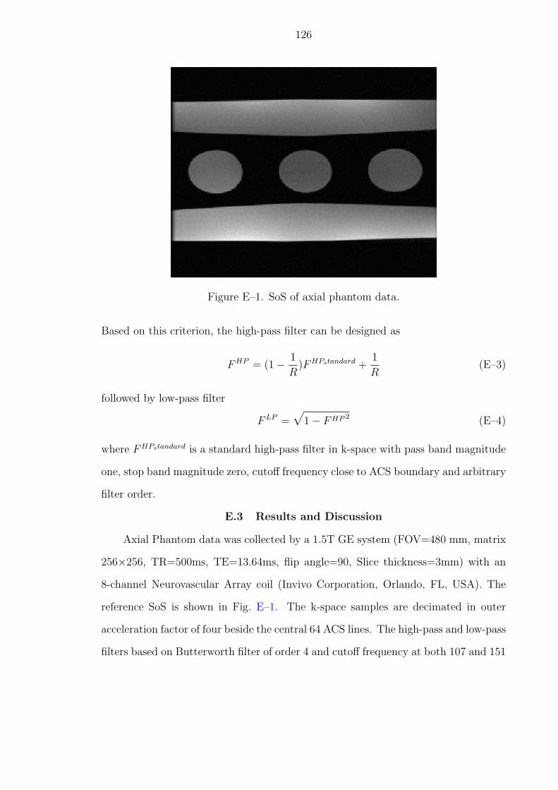
126

Figure E–1. SoS of axial phantom data.

Based on this criterion, the high-pass filter can be designed as

FHP = (1− 1

R)FHPstandard +

1

R(E–3)

followed by low-pass filter

FLP =√

1− FHP 2 (E–4)

where FHPstandard is a standard high-pass filter in k-space with pass band magnitude

one, stop band magnitude zero, cutoff frequency close to ACS boundary and arbitrary

filter order.

E.3 Results and Discussion

Axial Phantom data was collected by a 1.5T GE system (FOV=480 mm, matrix

256×256, TR=500ms, TE=13.64ms, flip angle=90, Slice thickness=3mm) with an

8-channel Neurovascular Array coil (Invivo Corporation, Orlando, FL, USA). The

reference SoS is shown in Fig. E–1. The k-space samples are decimated in outer

acceleration factor of four beside the central 64 ACS lines. The high-pass and low-pass

filters based on Butterworth filter of order 4 and cutoff frequency at both 107 and 151

127

Figure E–2. High-pass and low-pass filter with order 4 and cutoff frequency at 64.

are shown in Fig. E–2. The central PE line from the reconstructions using SENSE and

homoSENSE is demonstrated in Fig. E–3. It demonstrates that homoSENSE gives

less MSE compared to SENSE with less low frequency bias in the reconstruction.

The reconstruction time of both methods is about the same.

E.4 Conlusion

Variable density reconstruction processes full sampled and undersampled data in

parallel; but it is always affected by ring effect and combination bias. A filter design

criterion to suppress the bias is discussed in this short appendix. This global energy

balance criterion approximately solves the scale problem in final combination phase.

High and low-pass data are appropriately weighted and ringing is minimal.

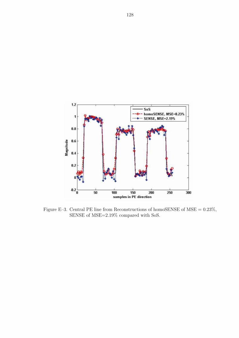
128

Figure E–3. Central PE line from Reconstructions of homoSENSE of MSE = 0.23%,SENSE of MSE=2.19% compared with SoS.

APPENDIX FHYBRID1DSENSE, A GENERALIZED SENSE RECONSTRUCTION

F.1 Introduction

Generalized k-space trajectories provide freedom of optimization either to in-

crease reconstruction SNR or to reduce aliasing. Generalized SENSE [101] provides

a global two dimensional solution to this problem by replacing the matrix inverse of

size N2 × N2, which has the computational load of O(N6), with a conjugate gradi-

ent (CG) thus the computational load reducing to O(LN3) given the image size and

epoch number L. SPACE RIP [99] and Generalized SMASH [100] further decompose

the 2D k-space into 1D k-space using SMASH modeling by solving the generalized

k-space trajectory problem in hybrid (k, r) space. This improvement reduces the

matrix size to N × N with the computational load O(N3) even without any itera-

tive algorithm. However, both methods incorporate modeling error when expressing

the coil sensitivities as linear combination of orthogonal sets. The proposed method,

named Hybrid1dSENSE, is to solve SENSE in hybrid (k, r) space by solving the in-

verse convolution equations, which avoids truncation errors as in [99, 100] and high

computational load in [101].

F.2 Method

The Hybrid1dSENSE originates from the fact that the coil image is a multiplica-

tion of the true NMR image and the coil sensitivity, which is equivalent to convolving

the Fourier transform of both NMR image and coil sensitivity. Since the undersam-

pled k-space data and the coil sensitivities are known a priori, the true NMR image

can be described as deconvolution with all coils.

129

130

Given a nc coil array with spatial coil sensitivity ci(x, y) and true MR image

ρ(x, y) where i = 1, · · · , nc, the acquired data in hybrid (k, r) space is given by

si(x, ky) =

∫ci(x, y)ρ(x, y) exp(−iyk)dy

= ci(x, ky)⊗ ρ(x, ky)

(F–1)

where x and ky is the frequency encoding (FE) direction in image space and the phase

encoding (PE) direction in k-space respectively, ci(x, ky) and ρ(x, ky) are the Fourier

transform of coil sensitivity ci(x, y) and ρ(x, y) at FE position x along PE line. Such

expression is reformulated in matrix form including multiple coil profiles as

s(x, ky) = P uρ(x, ky) (F–2)

where s(x, ky) = [s1(x, ky); · · · ; snc(x, ky)] is the undersampled hybrid space vec-

tor of size M1nc × 1 with M1 effective samples in PE direction of each coil image,

P u(x, ky) = [P u1(x, ky); · · · ; P unc(x, ky)] in which each element is a non-symmetric

Toeplitz matrix with ci(x, ky) in the first column and its (N − 1)th order circular left

shifted version in the first row. Thus a least square solution gives the hybrid space

reconstruction in Eqn. (F–3),

ρ(x, ky) = (P Hu P u)

−1P Hu s(x, ky) (F–3)

which gives the final reconstructed image followed by a 1D FFT.

F.3 Results and Discussion

Axial Phantom data is collected by a 1.5T GE system (FOV=480 mm, matrix

256×256, TR=500ms, TE=13.64ms, flip angle=90, Slice thickness=3mm) with an

8-channel Neurovascular Array coil (Invivo Corporation, Orlando, FL, USA). The

samples are decimated by an outer acceleration factor of four beyond the central

64 ACS lines. The reconstruction using equally space Cartesian SENSE and Hy-

brid1dSENSE is demonstrated in Fig. F.3. It demonstrates that Hybrid1dSENSE

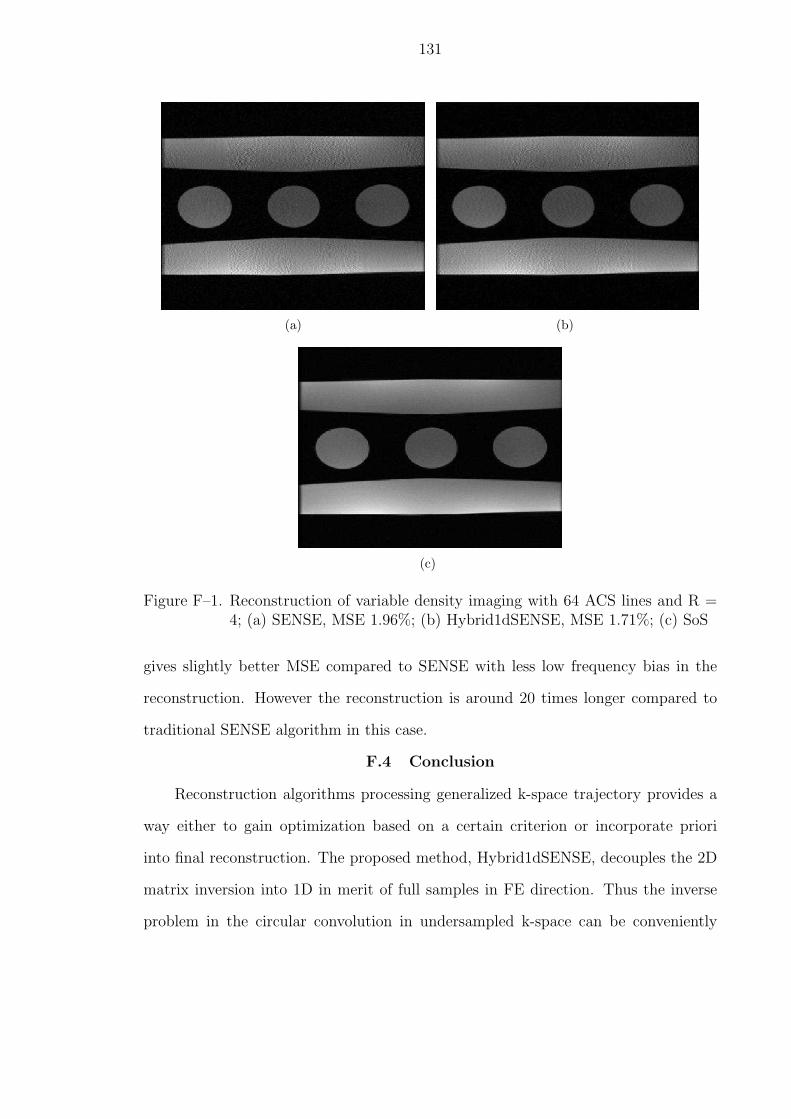
131

(a) (b)

(c)

Figure F–1. Reconstruction of variable density imaging with 64 ACS lines and R =4; (a) SENSE, MSE 1.96%; (b) Hybrid1dSENSE, MSE 1.71%; (c) SoS

gives slightly better MSE compared to SENSE with less low frequency bias in the

reconstruction. However the reconstruction is around 20 times longer compared to

traditional SENSE algorithm in this case.

F.4 Conclusion

Reconstruction algorithms processing generalized k-space trajectory provides a

way either to gain optimization based on a certain criterion or incorporate priori

into final reconstruction. The proposed method, Hybrid1dSENSE, decouples the 2D

matrix inversion into 1D in merit of full samples in FE direction. Thus the inverse

problem in the circular convolution in undersampled k-space can be conveniently

132

formulated into underdetermined least square solution in each coil. And further mul-

tiple coils balance this underdetermined issue by increasing times number of equations

while maintaining the same number of unknowns. The processing is time consuming

due to huge matrix inversion; however, parallel processing can dramatically reduce

the problem by increasing the processor complexity since each spatial location in FE

direction is decoupled already. Still, there’s room for improvement. The spatial local

redundancy of the image requires additional consideration either by 1D decomposition

with Markov Random Field (MRF) or 2D decomposition in further research.

APPENDIX GTRAJECTORY OPTIMIZATION IN K-T GRAPPA

G.1 Introduction

Dynamic imaging in MRI incorporates temporal correlation between frames.

Spatial resolution can be increased by sharing or interpolating information between

time frames. However, the practice can reduce temporal accuracy. Several recon-

struction methods have been proposed to exploit temporal correlation, e.g., UN-

FOLD [104], TSENSE [105], k-t BLAST and k-t SENSE [106] and k-t GRAPPA [107].

The further choice of sampling pattern in k-t space affects SNR, unwrapping artifact,

and temporal resolution. One desires to optimize the sampling pattern given a priori

knowledge of the image dynamics, such as breathing motion or contrast injection.

Tsao J. et al. give the optimal sampling patterns for k-t BLAST and k-t SENSE

by qualitatively analyzing the point spread function (PSF) in x-f space [108]. This

paper focuses on the optimization strategy applied to k-t GRAPPA and conjectures

a quantitative criterion for trajectory optimization. Parameters in the criterion can

be adjusted to accommodate spatial and temporal scales of change.

G.2 Method

k-t GRAPPA is a local spectrum interpolation strategy where the neighborhood

correlations both in PE encoding dimension and temporal dimension are extracted.

Missing k-space data points are estimated by convolution with a k-t kernel which is

calibrated adaptively in time. Since the reconstruction is a second order statistics

least square solution, the computational load is low. An example k-t trajectory is

demonstrated in Fig. G.3. We can see each periodic pattern is a square block of length

equal to the acceleration factor R and the acquired data are on the main diagonal

where all the off diagonal points are missing data ready to be estimated by the nearest

133

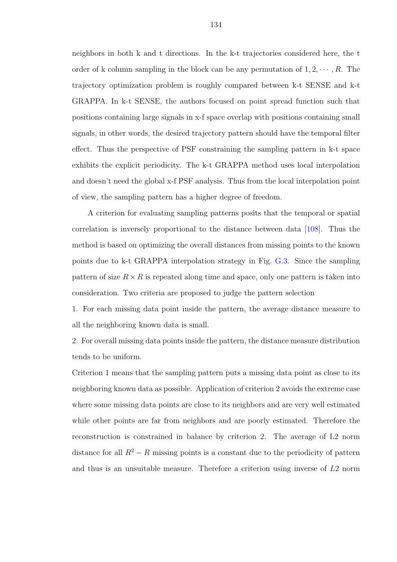
134

neighbors in both k and t directions. In the k-t trajectories considered here, the t

order of k column sampling in the block can be any permutation of 1, 2, · · · , R. The

trajectory optimization problem is roughly compared between k-t SENSE and k-t

GRAPPA. In k-t SENSE, the authors focused on point spread function such that

positions containing large signals in x-f space overlap with positions containing small

signals, in other words, the desired trajectory pattern should have the temporal filter

effect. Thus the perspective of PSF constraining the sampling pattern in k-t space

exhibits the explicit periodicity. The k-t GRAPPA method uses local interpolation

and doesn’t need the global x-f PSF analysis. Thus from the local interpolation point

of view, the sampling pattern has a higher degree of freedom.

A criterion for evaluating sampling patterns posits that the temporal or spatial

correlation is inversely proportional to the distance between data [108]. Thus the

method is based on optimizing the overall distances from missing points to the known

points due to k-t GRAPPA interpolation strategy in Fig. G.3. Since the sampling

pattern of size R×R is repeated along time and space, only one pattern is taken into

consideration. Two criteria are proposed to judge the pattern selection

1. For each missing data point inside the pattern, the average distance measure to

all the neighboring known data is small.

2. For overall missing data points inside the pattern, the distance measure distribution

tends to be uniform.

Criterion 1 means that the sampling pattern puts a missing data point as close to its

neighboring known data as possible. Application of criterion 2 avoids the extreme case

where some missing data points are close to its neighbors and are very well estimated

while other points are far from neighbors and are poorly estimated. Therefore the

reconstruction is constrained in balance by criterion 2. The average of L2 norm

distance for all R2 −R missing points is a constant due to the periodicity of pattern

and thus is an unsuitable measure. Therefore a criterion using inverse of L2 norm

135

Table G–1. k-t pattern comparison in k-t GRAPPA in reduction factor 4 cardiacimages.

[k,t] pattern [1,2,3,4] [1,2,4,3] [1,3,2,4] [1,3,4,2] [1,4,2,3] [1,4,3,2]RMSE 9.59% 10.49% 10.44% 10.45% 10.5% 9.56%

Crietrion 0.9242 0.9186 0.9186 0.9186 0.9186 0.9242

distance is proposed to evaluate the set of possible k-t trajectories in Eqn. (G–1),

maxpattern

α

√√√√ 1

R2 −R

R2−R∑n=1

(λx

∑k

1dn(kx)

+ λt

∑k

1dn(kt)

)α

maxn=1,··· ,R2−R(λx

∑k

1dn(kx)

+ λt

∑k

1dn(kt)

)α(G–1)

where λx and λt are the weighting factors in PE direction and temporal direction

corresponding to the spatial and temporal correlations separately, α is the order

of nonlinear transfer to adjust the distance distribution, dn(· ) defines the Euclidean

distance from missing data n to its nearest neighbors, kx and kt represents coordinates

in PE direction and temporal direction respectively.

G.3 Results and Discussion

Cardiac data was acquired using Siemens 8-channel cardiac array on 3T scanner

(TR=2; TI=100; TE=1.27; FOV=251×189; Flip Angle=12; Slice thickness=8mm;

matrix 192x88). The 70 fully acquired frames are decimated by different patterns in

acceleration factor of R=4, R=5 where 20 ACS lines are retained. Image sets are

reconstructed by k-t GRAPPA and compared to the fully sampled result to derive

a RMSE (Root Mean-Square-Error) for the pattern. Table G–1 demonstrates the

case R=4, where the optimal trajectories according to the optimization criterion

(λx = λt = 1, α = 2 for R = 4, 5) produce the lowest RMSE. Patterns [1, 2, 3, 4]

and [1, 4, 3, 2] have the highest criterion value. In the R = 5 case the trajectory

optimization criterion predicts optimal patterns of [13524] and [14253], corresponding

with the lowest RMSE values of 10.06% and 10.07% shown in Fig. G.3.

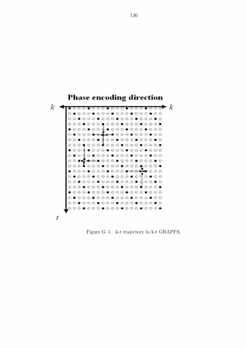
136

Figure G–1. k-t trajectory in k-t GRAPPA.

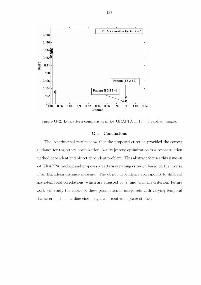
137

Figure G–2. k-t pattern comparison in k-t GRAPPA in R = 5 cardiac images.

G.4 Conclusions

The experimental results show that the proposed criterion provided the correct

guidance for trajectory optimization. k-t trajectory optimization is a reconstruction

method dependent and object dependent problem. This abstract focuses this issue on

k-t GRAPPA method and proposes a pattern searching criterion based on the inverse

of an Euclidean distance measure. The object dependence corresponds to different

spatiotemporal correlations, which are adjusted by λx and λt in the criterion. Future

work will study the choice of these parameters in image sets with varying temporal

character, such as cardiac cine images and contrast uptake studies.

REFERENCES

[1] F. Bloch, “Nuclear Induction,” Physical Review, vol. 70, pp. 460-474, 1946.

[2] E. M. Purcell, H. C. Torrey, and R. V. Pound, “Resonance Absorption byNuclear Magnetic Moments in a Solid,” Physical Review, vol. 69, p. 37, 1946.

[3] R. V. Damadian, “Tumor Detection by Nuclear Magnetic Resonance,” Science,vol. 171, p. 1151, 1971.

[4] P. C. Lauterbur, “Image Formation by Induced Local Interactions: ExamplesEmploying Nuclear Magnetic Resonance,” Nature, vol. 242, pp. 190-191, 1973.

[5] A. Kumar, D. Welti, R. R. Ernst, “NMR Fourier Zeugmatography,” Journalof Magnetic Resonance, vol. 18, pp. 69-83, 1975.

[6] P. A. Bandettini, E. C. Wong, R. S. Hinks, R. S. Tikofsky, J. S. Hyde, “TimeCourse EPI of Human Brain Function during Task Activation,” Magnetic Res-onance in Medicine, vol. 25, pp. 390-397, 1992.

[7] P. A. Tataranni, J-F Gautier, K. Chen, A. Uecker, D. Bandy, A. D. Salbe,R. E. Pratley, M. Lawson, E. M. Reiman, and E. Ravussin, “Neuroanatom-ical Correlates of Hunger and Satiation in Humans using Positron EmissionTomography,” Proceedings of National Academy of Science, vol. 96, issue 8,pp. 4569-4574, 1999.

[8] Y. Liu, J.-H. Gao, M. Liotti, Y. Pu, and P. T. Fox, “Temporal Dissociationof Parallel Processing in the Human Subcortical Outputs,” Nature, vol. 400,pp. 364-367, 1999.

[9] Y. Liu, J-H Gao, H-L Liu and P. T. Fox, “The Temporal Response of the Brainafter Eating Revealed by Functional MRI,” Nature, vol. 405, pp. 1058-1062,2000.

[10] P. B. Roemer, W. A. Edelstein, C. E. Hayes, S. P. Souza and O. M. Mueller,“The NMR Phased Array,” Magnetic Resonance in Medicine, vol. 16, pp. 192-225, 1990.

[11] K. P. Pruessmann, M. Weiger, M. B. Scheidegger, P. Boesiger, “SENSE: Sen-sitivity Encoding for Fast MRI,” Magnetic Resonance in Medicine, vol. 42,pp. 952-962, 1999.

138

139

[12] J. A. Bankson, M. A. Griswold, S. M. Wright, D. K. Sodickson, “SMASH Imag-ing with An Eight Element Multiplexed RF Coil Array,” Magnetic ResonanceMaterials in Physics, Biology and Medicine (MAGMA), vol. 10, pp. 93-104,2000.

[13] J. P. Debbins, J. P. Felmlee, S. J. Riederer, “Phase Alignment of MultipleSurface Coil Data for Reduced Bandwidth and Reconstruction Requirements,”Magnetic Resonance in Medicine, vol. 38, pp. 1003-1011, 1997.

[14] D. O. Walsh, A. F. Gmitro, M. W. Marcellin, “Adaptive Reconstruction ofPhased Array MR Imagery,” Magnetic Resonance in Medicine, vol. 43, pp. 682-690, 2000.

[15] P. Kellman, E. R. McVeigh, “Ghost Artifact Cancellation using Phased ArrayProcessing,” Magnetic Resonance in Medicine, vol. 46, pp. 335-343, 2001.

[16] M. Bydder, D. J. Larkman, J. V. Hajnal, “Combination of Signals from ArrayCoils Using Image-Based Estimation of Coil Sensitivity Profiles,” MagneticResonance in Medicine, vol. 47, pp. 539-548, 2002.

[17] R. Yan, D. Erdogmus, E. G. Larsson, J. C. Principe and J. R. Fitzsimmons,“Image Combination for High-Field Phased-Array MRI,” Proceedings of IEEEConference on Acoustics, Speech, and Signal Processing, 2003, Hong Kong,China, vol. 5, pp. 6-10, Apr. 2003.

[18] M. A. Griswold, P. M. Jakob, M. Nittka, J. W. Goldfarb, and A. Haase, “Par-tially Parallel Imaging with Localized Sensititivities(PILS),” Magnetic Reso-nance in Medicine, vol. 44, pp. 602-609, 2000.

[19] J. W. Goldfarb, and A. E. Holland, “Parallel Magnetic Resonance Imagingusing Coils with Localized Sensitivities,” Magnetic Resonance Imaging, vol. 22,no. 7, pp. 1025-1029, Sep. 2004.

[20] J. P. Hornak, The Basics of MRI, Interactive Learning Software, Henrietta,NY, 2004.

[21] E. M. Haacke, R. W. Brown, M. R. Thompson, and R. Venkatesan, MagneticResonance Imaging - Physical Principles and Sequence Design, John Wiley &Sons, Inc., New York, NY, 1999.

[22] W. A. Edelstein , G. H. Glover, C. J. Hardy, and R. W. Redington, “The Intrin-sic Signal-to-Noise Ratio in NMR Imaging,” Magnetic Resonance in Medicine,vol. 3, pp. 604-618, 1986.

[23] C. E. Hayes and P. B. Roemer, “Noise Correlations in Data SimultaneouslyAcquired from Multiple Surface Coil Arrays,” Magnetic Resonance in Medicine,vol. 16, pp. 181-191, 1990.

140

[24] G. R. Duensing, H. R. Brooker HR, and J. R. Fitzsimmons, “MaximizingSignal-to-Noise Ratio in the Presence of Coil Coupling,” Journal of MagneticResonance, vol. 111, pp. 230-235, 1996.

[25] R. A. Horn and C. R. Johnson, Matrix Analysis, Cambridge University Press,Cambridge, MA, 1985.

[26] S. M. Wright, L. L. Wald, “Theory and Application of Array Coils in MRSpectroscopy,” NMR in Biomedicine, vol. 10, pp. 394-410, 1997.

[27] S. M. Kay, Fundamentals of Statistical Signal Processing: Estimation Theory,Prentice Hall, Englewood Cliffs, NY, 1993.

[28] E. G. Larsson, D. Erdogmus, R. Yan, J. C. Principe and J. R. Fitzsimmons,“SNR-Optimality of Sum-of-Squares Reconstruction for Phased-Array Mag-netic Resonance Imaging,” Journal of Magnetic Resonance, vol. 163, no. 1,pp. 121-123, Jul. 2003.

[29] A. Papoulis, Probability, Random Variables, and Stochastic Processes,McGraw-Hill, New York, NY, 1991.

[30] K. S. Yee, “Numerical Solution of Initial Boundary Value Problems InvolvingMaxwells Equations in Isotropic Media,” IEEE Trans., Antennas and Propa-gation, vol. 14, pp. 302-307, 1996.

[31] K. S. Kunz and R. J. Luebbers, The Finite Difference Time Domain Methodfor Electromagnetics, CRC Press, Boca Raton, FL, 1993.

[32] T. S. Ibrahim, R. Lee, B. A. Baertlein, A. Kangarlu, and P. M. L. Robitaille,“Application of Finite-Difference Time-Domain Method for the Design of Bird-cage RF Head Coils Using Multi-Port Excitations,” Magnetic Resonance inMedicine, vol. 18, pp. 733-742, 2000.

[33] F-H Lin, Y-J Chen, J. W. Belliveau, and L. L. Wald, “Removing Signal Inten-sity Inhomogeneity from Surface Coil MRI using Diescrete Wavelet Transformand Wavelet Packet,” Proceedings of the 23rd Annual EMBS InternationalConference of the IEEE, Istanbul, Turkey, 2001, vol. 3, pp. 2793-2796.

[34] H. Vesselle and R. E. Collin, “The Signal-to-Noise Ratio of Nuclear MagneticResonance Surface Coils and Application to a Lossy Dielectric Cylinder Model-Part I: Theory,” IEEE Trans., Biomedical Engeneering, vol. 42, no. 5, pp. 497-506, 1995.

[35] D. I. Hoult and R. E. Richards, “The Signal-to-Noise Ratio of the NuclearMagnetic Resonance Experiment,” Journal of Magnetic Resonance, vol. 24,pp. 71-85, 1976.

141

[36] X. Tang, “Multiple Competitive Learning Network Fusion for Object Classifi-cation,” IEEE Trans., Systems, Man and Cybernetics, Part B, vol. 28, no. 4,pp. 532-543, Aug. 1998.

[37] S. C. Ahalt, A. K. Krishamurthy, P. Chen, and D. E. Melton, “CompetitiveLearning Algorithms for Vector Quantization,” Neural Networks, vol. 3, pp. 277-290, 1990.

[38] T. M. Martinetz, S. G. Berkovich, and K. J. Schulten, “’Neural-Gas’ Networkfor Vector Quantization and Its Application to Time-Series Prediction,” NeuralNetworks, vol. 4, no. 4, pp. 558-569, 1993.

[39] D. Rumelhart and D. Zipser, “Feature Discovery by Competitive Learning,”Cognitive Science, vol. 9, pp. 75-112, 1985.

[40] A. S. Galanopoulos, R. L. Moses and S. C. Ahalt, “Diffusion Approximationof Frequency Sensitive Competitive Learning,” IEEE Trans. Neural Networks,vol. 8, no. 5, pp. 1026-1030, Sep. 1997.

[41] T. Kohonen, “The Self-Organizing Map,” Proc. IEEE, vol. 78, no. 9, pp. 1464-1480, Sep. 1990.

[42] W. C. Fang, B. J. Sheu, O. T. C. Chen, and J. Choi, “A VLSI Neural Processorfor Image Data Compression using Self-Organization Network,” IEEE Trans.Neural Networks, vol. 3, no. 3, pp. 506-518, May 1992.

[43] T. Uchiyama, and M. A. Arbib, “Color Image Segmentation Using competitiveLearning,” IEEE Trans. Pattern Analysis and Machine Intelligence, vol. 16,no. 12, pp. 1197-1206, Dec. 1994.

[44] P. Schunders, “Joint Quantisation and Error Diffusion of Colour Images Us-ing Competitive Learning,” IEE Proc. Vision, Image and Signal Processing,vol. 145, no. 2, pp. 137-140, Apr. 1998.

[45] E. Alpaydin and M. I. Jordan, “Local Linear Perceptrons for Classification,”IEEE Trans. Neural Networks, vol. 7, no. 3, pp. 788-794, May 1996.

[46] J. D. Farmer and J. J. Sidorowich, “Predicting Chaotic Time Series PhysicalReview Letters,” Phys. Rev. Lett., vol. 59, no. 8, pp. 845-848, 1987.

[47] J. C. Principe, Ludong Wang and M. A. Motter, “Local Dynamic Modelingwith Self-Organizing Maps and Applications to Nonlinear System Identificationand Control,” Proc. IEEE, vol. 86, no. 11, pp. 2240-2258, Nov. 1998.

[48] A. C. Singer, G. W. Wornell, A. V. Oppenheim, “Codebook Prediction: aNonlinear Signal Modeling Paradigm,” Proceedings of IEEE Conference onAcoustics, Speech, and Signal Processing 1992, San Francisco, CA, 1992, vol. 5,pp. 325-328.

142

[49] R. A. Jacobs, M. I. Jordan, S. J. Nowlan and G. E. Hinton, “Adaptive Mixturesof Local Experts,” Neural Computation, vol. 3, pp. 79-87, 1991.

[50] C. L. Fancourt, “Gated Competitive Systems for Unsupervised Segmenta-tion and Modeling of Piecewise Stationary Signals,” PhD thesis, Universityof Florida, 1998.

[51] L. Bottou and V. N. Vapnik, “Local Learning Algorithms,” Neural Computa-tion, vol. 4, pp. 888-900, 1992.

[52] R. Murray-Smith and T. A. Johansen, “Local Model Networks and Local Learn-ing,” Multiple Model Approaches to Modelling and Control, pp. 185-210, Taylorand Francis, 1997.

[53] C. K. Loo and M. Rajeswari, “Growing Multi-Experts Network,” TENCON2000, Proceedings, Kuala Lumpur, Malaysia, 2000, vol. 3, pp. 472-477.

[54] S. Haykin, Adaptive Filter Theory, Pearson Education Inc., Delhi, India, 2002.

[55] S. Haykin, Neural Networks, a Comprehensive Foundation, Pearson EducationInc., Delhi, India, 2002.

[56] D. Erdogmus, “Information Theoretic Learning: Renyi’s Entropy and Its Appli-cations to Adaptive System Training,” PhD Dissertation, University of Florida,2002.

[57] S. Zola-Morgan, “Localization of Brain Function: the Legacy of Franz JosephGall (1758-1828),” Annual Review Neuroscience, vol. 18, pp. 359-383, 1995.

[58] O. Friman, J. Cedefamn, P. Lundberg, M. Borga, and H. Knutsson, “Detectionof Neural Activity in Functional MRI using Canonical Correlation Analysis,”Magnetic Resonance in Medicine, vol. 45, pp. 323-330, 2001.

[59] D. Gembris, G. G. Taylor, S. Schor, W. Frings, D. Suter, and S. Posse, “Func-tional Magnetic Resonance Imaging in Real Time (FIRE): Slidingwindow Cor-relation Analysis and Reference-vector Optimization,” Magnetic Resonance inMedicine, vol. 43, pp. 259-268, 2000.

[60] A. H. Anderson, D. M. Gash, and M. J. Avison, “Principal Component Analysisof the Dynamic Response Measured by fMRI: A Generalized Linear SystemsFrameworks,” Magnetic Resonance Imaging, vol. 17, pp. 795-815, 1999.

[61] R. Baumgartner, L. Ryner, W. Richter, R. Summers, M. Jarmasz, and R.Somorjai, “Comparison of Two Exploratory Data Analysis Methods for fMRI:Fuzzy Clustering vs. Principal Component Analysis,” Magnetic Resonance inMedicine, vol. 18, pp. 89-94, 2000.

143

[62] V. D. Calhoun, T. Adali, G. D. Pearlson, and J. J. Pekar, “A Method for MakingGroup Inferences from Functional MRI Data using Independent ComponentAnalysis,” Human Brain Mapping, vol. 14, pp. 140-151, 2001.

[63] M. J. McKeown, S. Makeig, G. G. Brown, T. P. Jung, S. S. Kindermann, A. J.Bell, and T. J. Sejnowski, “Analysis of fMRI Data by Blind Separation intoIndependent Spatial Components,” Human Brain Mapping, vol. 6, pp. 160-188,1998.

[64] E. Salli, H. J. Aronen, S. Savolinen, A. Corvenoja, and A. Visa, “Contex-tual clustering for Analysis of Functional MRI Data,” Medical Imaging, IEEETransactions, vol. 20, pp. 403-414, 2001.

[65] A. Baune, F. T. Sommer, M. Erb, D. Wildgruber, B. Kardatzki, G. Palm,and W. Grodd, “Dynamical Cluster Analysis of Cortical fMRI Activation,”NeuroImage, vol. 9, pp. 477-489, 1999.

[66] C. Goutte, P. Toft, E. Rostrup, F. A. Nielsen, and L. K. Hansen, “On ClusteringfMRI Time Series,” NeuroImage, vol. 9, pp. 298-310, 1999.

[67] K. J. Friston, P. Jezzard and R. Turner, “Analysis of Functional MRI Time-series,” Human Brain Mapping, vol. 1, pp. 153-171, 1994.

[68] S.-C. Ngan and X. Hu, “Analysis of Functional Magnetic Resonance ImagingData using Self-organizing Mapping with Spatial Connectivity,” Magnetic Res-onance in Medicine, vol. 41, pp. 939-946, 1999.

[69] S-H Seo, and M. R. Azimi-Sadjadi, “Orthogonal Subspace Projectionn Filteringfor Stereo Image Compression,” Proceedings IEEE International Conference onAcoustics, Speech and Signal Processing, Seattle, WA, 1998, vol. 5, pp. 2577-2580.

[70] C-I Chang, X. L. Zhao, M.L.G. Althouse, and J. J. Pan, “Least Squares Sub-space Projection Approach to Mixed Pixel Classification for Hyperspectral Im-ages,” Geoscience and Remote Sensing, IEEE Transactions, vol. 2, pp. 69-79,1994.

[71] S. Haykin, Neural Networks: A Comprehensive Foundation, Macmillan, NewYork, NY, 1994.

[72] T. K. Leen and N. Kambhatla, “Fast Non-Linear Dimension Reduction,” Ad-vances in Neural Information Processing Systems, vol. 6, pp. 152-159, 1994.

[73] N. Kambhatla and T. K. Leen, “Dimension Reduction by Local Principal Com-ponent Analysis,” Neural Computation, vol. 9, pp. 1493, 1997.

[74] R. D. Dony and S. Haykin, “Optimally Adaptive Transform Coding,” ImageProcessing, IEEE Transactions, vol. 4, pp. 1358-1370, 1995.

144

[75] C. L. Fancourt, and J. C. Principe, “Soft Competitive Principal Compo-nent Analysis Using the Mixture of Experts,” PhD Dissertation, Universityof Florida, 1998.

[76] D. D. Lee and H. S. Seung, “Learning the Parts of Objects by Non-negativeMatrix Factorization,” Nature, vol. 401, pp. 788-791, 1999.

[77] D. D. Lee and H. S. Seung, “Algorithms for Non-negative Matrix Factorization,”In Advances in Neural Information Processing Systems, vol. 13, pp. 556-562,2001.

[78] R. D. Dony, and S. Haykin, “Neural Netowrk Approaches to Image Compres-sion,” Proceedings of the IEEE, vol. 83, pp. 288-303, 1995.

[79] E. McVeigh and C. Ozturk, “Imaging Myocardial Strain,” IEEE Signal Process-ing Magazine, pp. 44-56, Nov. 2001.

[80] W. K. Pratt, Digital Image Processing, John Wiley and Sons, Inc., New York,NY, 1978.

[81] G. McGibney and M. R. Smith, “An Unbiased Signal-to-noise Ratio Measurefor Magnetic Resonance Images,” Medical Physics, vol. 20, no. 4, pp. 1077-1078,1992.

[82] R. M. Henkelman, “Measurement of Signal Intensities in the Presence of Noisein MR Images,” Medical Physics, vol. 12, pp. 232-233, 1985.

[83] R. M. Henkelman and M. J. Bronskill, “Artifacts in Magnetic Resonance Imag-ing,” Reviews of Magnetic Resonance in Medicine, vol. 2, pp. 1-126, 1987.

[84] C. D. Constantinides, E. Atalar and E. R. McVeigh, “Signal-to-noise Measure-ments in Magnitude Images from NMR Phased Arrays,” Magnetic Resonancein Medicine, vol. 38, pp. 852-857, 1997.

[85] H. Gudbjartsson and S. Patz, “The Rician Distribution of Noisy MRI Data,”Magnetic Resonance in Medicine, vol. 34, pp. 910-914, 1995.

[86] B. L. Beck and S. J. Blackband, “Phased Array Imaging on a 4.7T/33cm AnimalResearch System,” Review of Scientific Instruments, vol. 72, no. 11, pp. 4292-4294, 2001.

[87] Q. Zhao, J. C. Principe, J. Fitzsimmons, M. Bradley and P. Lang, “Func-tional Magnetic Resonance Imaging Data Analysis with Information-theoreticApproaches,” Chapter 9, Biocomputing, edited by P. Pardalos and J. Principe,Kluwer Academic Publishers, Dordrecht, The Netherlands, 2002

[88] H. H. Barrett, J. Yao, J. P. Rolland, and K. J. Myers, “Model Observers forAssessment of Image Quality,” Proceedings of the National Academy of Sciences,vol. 90, pp. 9758-9765, 1993.

145

[89] W. E. Smith and H. H. Barrett, “Hotelling Trace Criterion as a Figure of Meritfor the Optimization of Imaging Systems,” Journal of the Optical Society ofAmerica, vol. 3, pp. 717-725, 1986.

[90] K. J. Myers and H. H. Barrett, “Addition of a Channel Mechanism to the Ideal-observer Model,” Journal of the Optical Society of America, vol. 4, pp. 2447-2457, 1987.

[91] T. W. Redpath, “Signal-to-noise Ratio in MRI,” The British Journal of Radi-ology, vol. 71, pp. 704-707, 1998.

[92] T. W. Redpath and C. J. Wiggins, “Estimating Achievable Signal-to-noise Ra-tios of MRI Transmit-receive Coils from Radiofrequency Power Measurements:Applications in Quality Control,”. Physics in Medicine and Biology, vol. 45,pp. 217-227, 2000.

[93] M. J. Firbank, R. M. Harrison , E. D. Williams and A. Coulthard, “Qual-ity Assurance for MRI: Practical Experience,” The British Journal of Radiol-ogy,vol. 73, pp. 376-383, 2000.

[94] D. Erdogmus, E. G. Larsson, R. Yan, J. C. Principe and J. R. Fitzsim-mons, “Measuring the Signal-to-noise Ratio in Magnetic Resonance Imaging: aCaveat,” Signal Processing, vol. 84, no. 6, pp. 1035-1040, 2004.

[95] J. Sijbers, A. den Dekker, J. van Audekerke, M. Verhove and D. van Dyck, “Es-timation of the Noise in Magnitude MR Images,” Magnetic Resonance Imaging,vol. 16, pp. 87-90, 1998.

[96] M. J. Firbank, A. Coulthard, R. M. Harrison and E. D. Williams, “A Compar-ison of Two Methods for Measuring the Signal to Noise Ratio on MR Images,”Physics in Medicine and Biology, vol. 44,pp. 261-264, 1999.

[97] L. Kaufman, D. M. Kramer, L. E. Crooks and D. A. Ortendahl, “MeasuringSignal to Noise Ratios in MR Imaging Radiology,” vol. 173, pp. 265-267, 1989.

[98] A. V. Oppenheim and R. W. Schafer, Digital Signal Processing, Prentice HallInc., Englewood Cliffs, NY, 1975.

[99] W. E. Kyriakos, L. P. Panych, D. F. Kacher, C-F Westin, S. M. Bao, R. V.Mulkern, and F. A. Jolesz, “Sensitivity Profiles From an Array of Coils forEncoding and Reconstruction in Parallel (SPACE RIP),” Magnetic Resonancein Medicine, vol. 44, pp. 301-308, 2000.

[100] M. Bydder, D. J. Larkman and J. V. Hajnal, “Generalized SMASH Imaging,”Magnetic Resonance in Medicine vol. 47, pp. 160-170, 2002.

[101] K. P. Pruessmann, M. Weiger, P. Bornert, and P. Boesiger, “Advances in Sen-sitivity Encoding With Arbitrary k-Space Trajectories,” Magnetic Resonancein Medicine,vol. 46, pp. 638-651, 2001.

146

[102] B. Madore, “UNFOLD-SENSE: A Parallel MRI Method With Self- Calibrationand Artifact Suppression,” Magnetic Resonance in Medicine vol. 52, pp. 310-320, 2004.

[103] K. F. King, “Efficient Variable Density SENSE Reconstruction,” Proceedingsof International Society for Magnetic Resonance in Medicine, Miami, Fl, 2005,vol. 13, p. 2418.

[104] B. Madore, G. H. Glover and N. J. Pelc, “Unaliasing by Fourier-Encodingthe Overlaps Using the Temporal Dimension (UNFOLD), Applied to CardiacImaging and fMRI,” Magnetic Resonance in Medicine, vol. 42, pp. 813-828,1999.

[105] P. Kellman, F. H. Epstein and E. R. McVeigh, “Adaptive Sensitivity EncodingIncorporating Temporal Filtering (TSENSE),” Magnetic Resonance in Medi-cine, vol. 45, pp. 846-852, 2001.

[106] M. S. Hansen, S. Kozerke, K. P. Pruessmann, P. Boesiger, E. M. Pedersen, andJ. Tsao, “On the Influence of Training Data Quality in k-t BLAST Reconstruc-tion,” Magnetic Resonance in Medicine, vol. 52, pp. 1175-1183, 2004.

[107] F. Huang, J. Akao, S. Vijayakumar, G. R. Duensing and M. Limkeman, “k-tGRAPPA: A k-space Implementation for Dynamic MRI with High ReductionFactor Magnetic Resonance in Medicine,” Magnetic Resonance in Medicine,vol. 54, pp. 1172-1184, 2005.

[108] J. Tsao, S. Kozerke, P. Boesiger and K. P. Pruessmann, “Optimizing Spa-tiotemporal Sampling for k-t BLAST and k-t SENSE: Application to High-Resolution Real-Time Cardiac Steady-State Free Precession,” Magnetic Reso-nance in Medicine, vol. 53, pp. 1372-1382, 2005.

BIOGRAPHICAL SKETCH

Rui Yan was born in Chongqing, China, on January 1st, 1978. He received his

B.E. degree in the Department of Wireless Communications from Beijing University

of Posts and Telecommunications, in 1999. He continued his graduate study in the

Training Center from Beijing University of Posts and Telecommunications between

1999-2000 and in the Department of Electrical and Computer Engineering from the

Old Dominion University between 2000–2001. In 2001, he joined the Department

of Electrical and Computer Engineering at the University of Florida to pursue a

Ph.D. in machine learning and medical imaging with a M.S. degree obtained in 2003.

Under the guidance of Dr. Jose C. Principe in the Computational NeuroEngineering

Laboratory, his research is mainly focused on adaptive signal processing applied to

medical imaging. He is a member of the IEEE Signal Processing Society and also a

student member of the IEEE.

147

competitive mixture of local linear experts for magnetic

Documents

Transcript of competitive mixture of local linear experts for magnetic