A dimensionally reduced finite mixture model for multilevel data

Journal of Multivariate Analysis 101 (2010) 2543–2553

Contents lists available at ScienceDirect

Journal of Multivariate Analysis

journal homepage: www.elsevier.com/locate/jmva

A dimensionally reduced finite mixture model for multilevel dataDaniela G. Calò ∗, Cinzia ViroliDepartment of Statistics, University of Bologna, via Belle Arti, 41, Bologna, Italy

a r t i c l e i n f o

Article history:Received 9 July 2009Available online 23 July 2010

AMS subject classifications:primary 62H30secondary 62H25

Keywords:Cluster analysisFactor mixture modelDimension reductionEM-algorithmMultilevel latent class analysis

a b s t r a c t

Recently, different mixture models have been proposed for multilevel data, generallyrequiring the local independence assumption. In this work, this assumption is relaxed byallowing each mixture component at the lower level of the hierarchical structure to bemodeled according to a multivariate Gaussian distribution with a non-diagonal covariancematrix. For high-dimensional problems, this solution can lead to highly parameterizedmodels. In this proposal, the trade-off betweenmodel parsimony and flexibility is governedby assuming a latent factor generative model.

© 2010 Elsevier Inc. All rights reserved.

1. Introduction

Multilevel data are collected in different applied fields of research, such as sociology, behavioral science and medicine.Data from students nested within schools or patients hospitalized in different primary care centers are typical examplesof two-level data: pupils and patients are referred to as lower level units, while being schools and hospitals the respectivehigher level units. A two-level multivariate data set, where multiple responses are recorded for each lower level unit, canalso be seen as a three-level data set by interpreting multivariate responses as nested univariate responses.Different models have been proposed for describing multilevel data (see, for example, [17,18]). Recently, various types

of latent class [9] and finite mixture models [13] for data sets having a multilevel structure have been proposed (see, forexample, [20,21]). In particular, Vermunt [19,22] and Vermunt and Magidson [24] have introduced a hierarchical extensionof these two model-based clustering methods, with the aim of clustering multilevel data on the basis of a set of categoricalor continuous response variables. As in standard model-based clustering, the main goal of their proposal is to build ameaningful cluster model for the lower level units. However, in order to take the nested data structure into account, certainmodel parameters are allowed to differ randomly across higher level units. A particular variant—that is dealt with in thepresent paper—is based on the introduction of a discrete random effect that is assumed to capture higher level variation inlower level class membership probabilities. Since this amounts to assume that higher level units belong to a given numberof latent classes, the resulting multilevel model contains a separate finite mixture distribution at each level of nesting, thusyielding a simultaneous model-based clustering of units at both the levels of the hierarchy.The above-mentioned multilevel mixture model is presented in [22] by making the additional assumption that the

observed responses are conditionally independent of one another given the class membership of the generic lower levelunit (which is sometimes referred to as the local independence assumption). If the observed variables are modeled as afinite Gaussian mixture, this amounts to assume all the component covariance matrices to be diagonal. By removing such a

∗ Corresponding author.E-mail address: [email protected] (D.G. Calò).

0047-259X/$ – see front matter© 2010 Elsevier Inc. All rights reserved.doi:10.1016/j.jmva.2010.07.003

http://www.elsevier.com/locate/jmva

http://www.elsevier.com/locate/jmva

mailto:[email protected]

http://dx.doi.org/10.1016/j.jmva.2010.07.003

2544 D.G. Calò, C. Viroli / Journal of Multivariate Analysis 101 (2010) 2543–2553

constraint,more flexiblemodels can be defined. On the other hand, a fully unconstrained parameterization of the componentcovariance matrices involves a quadratic increasing number of parameters as dimensionality increases. When dealing withhigh-dimensional data, this choice could lead to unreliable estimates or to over-fitting problems.An alternative method for dealing with local dependencies can be devised by interpreting a two-level multivariate data

set as a three-level data set, with response variables representing the lowest level units in the hierarchy. It consists inintroducing one (or more) continuous latent variable(s) in the lowest level of hierarchy (see [23], Section 3.3).In the present paper, a specific mixture model belonging to this latter methodological framework is proposed that weak-

ens the local independence assumption while governing the trade-off between model flexibility and parsimony. It repre-sents the multilevel variant of the Heteroscedastic Factor Mixture Model (HFMM), which has been introduced by Montanariand Viroli [14] as an effective method for dimensionally reduced model-based clustering.The basic idea is to assume that the p response variables are generated by q latent factors (with q < p), which are jointly

distributed as a finite Gaussian mixture. Under these conditions, it can be proved that the observed variables are modeledas a finite Gaussian mixture as well, with parameters depending on the parameters of the factor distribution. In so doing,the number of model parameters is controlled via the dimensionality of the reduced latent space; in addition, the latentvariables can provide useful information for better understanding the investigated phenomenon.The remainder of the paper is organized as follows. After introducing some preliminaries in the next section, Section 3

provides a short description of the hierarchical finite mixturemodel for nested data developed in [24,22]. Section 4 presentsthe proposed clustering model and describes the restrictions needed for its identification. In Section 5, maximum likelihoodestimation of model parameters via the EM algorithm is developed. Section 6 presents the classification performance of theproposed model on artificial two-level multivariate data sets with varying higher level clustering structures; moreover, areal data example is illustrated where the proposedmodel provides a meaningful and relatively more parsimonious model-based clustering.

2. Preliminaries

The multilevel models described in the following two sections deal with two-level p-variate data. However, three-leveldata notation and terminology will be used in their formulation since multivariate responses are conceived as nestedunivariate responses (which yields an extra level of nesting). For example, multivariate data observed on students nestedwithin schools can be viewed in a hierarchical structure where third-level units are schools, second-level units are studentsand first-level units are the univariate responses nested within each student.First-level units are referred to by the index h, ranging from 1 to p, second-level units are denoted by the index i, and

third-level units are labeled by the index j, with j = 1, . . . , J . The number of second-level units within third-level unit j isdenoted by nj, where

∑Jj=1 nj = n.

Let yhij ∈ R denote the value of the hth observed variable for second-level unit i within third-level unit j. Notationyij = [yhij]h=1,...,p is used to refer to the p-dimensional vector of responses for case iwithin third-level unit j.

3. Hierarchical finite mixture model

The model proposed in [24,22] allows a simultaneous model-based clustering of third-level units into L latent classesand second-level units into K latent classes. Both L and K are assumed to be fixed but unknown. In the following, the twocorresponding latent class variables will be represented as allocation vectors: namely, sj = [sjl]l=1,...,L and rij = [rijk]k=1,...,Kfor third-level and second-level units, respectively. More specifically, with reference to a (second- or third-level) unit, thegeneric component of an allocation vector takes value 1 in correspondence of the class the unit belongs to, and 0 otherwise.The model consists of the following two parts:

f (yj) =L∑l=1

wl

nj∏i=1

f (yij|sj1 = 0, . . . , sjl = 1, . . . , sjL = 0) (1)

f (yij|sj1 = 0, . . . , sjl = 1, . . . , sjL = 0) =K∑k=1

πk|lf (yij|rij1 = 0, . . . , rijk = 1, . . . , rijK = 0), (2)

where sj ∼ B(1;w1, . . . , wl, . . . , wL) and rij|(sj1 = 0, . . . , sjl = 1, . . . , sjL = 0) ∼ B(1;π1|l, . . . , πk|l, . . . , πK |l), withB(1; . . .) denoting the multinomial distribution with number of trials equal to 1.In Eq. (1), third-level units are assumed to belong to one of L latent classes with prior probabilities equal to wl (where∑Ll=1wl = 1), and observations within third-level unit j are assumed to be mutually independent given the class

membership of unit j.In Eq. (2), the conditional density f (yij|sj) is modeled as a finite mixture: second-level units within third-level unit j

are assumed to belong to one of K latent classes with prior probabilities equal to πk|l (where∑Kk=1 πk|l = 1). These latter

probabilities depend on the class membership of unit j, whereas the component densities are assumed to not differ acrossthird-level classes.

D.G. Calò, C. Viroli / Journal of Multivariate Analysis 101 (2010) 2543–2553 2545

Finally, in the model defined by (1) and (2) the parameters {πk|l, k = 1, . . . , K} are allowed to differ randomly acrossthird-level units, according to the discrete random effect described by sj ∼ B(1;w1, . . . , wl, . . . , wL).In the case of finite mixtures of Gaussian distributions, Eq. (2) takes the following form:

f (yij|sj1 = 0, . . . , sjl = 1, . . . , sjL = 0) =K∑k=1

πk|lφ(p)k (yij;µk,6k), (3)

where φ(p)k denotes the p-dimensional Gaussian density with mean µk and covariance matrix 6k. Under the local indepen-dence assumption, the responses are taken to be mutually independent given rij, then Eq. (3) simplifies to

f (yij|sj1 = 0, . . . , sjl = 1, . . . , sjL = 0) =K∑k=1

πk|l

p∏h=1

φ(1)k (yhij;µhk, σ

2hk). (4)

Maximum likelihood estimates of the parameters of model (1)–(2) can be obtained by an adapted EM algorithm [6] thathas been implemented in the Latent GOLD software package [25]. Then, the units of both levels can be partitioned intoclusters according to the criterion of the maximum estimated posterior class membership probability.

4. The proposed model

The proposed model includes the same two parts described in Eqs. (1) and (2), but contains a further part that serves toconnect the p responses (i.e. first-level units) observed on the same second-level unit. This connection is described through agenerative factormodel involving q latent variables (with q < p). Therefore, themodel involves not only the two latent classvariables s and r introduced in Section 3, but also a further q-dimensional continuous latent variable linked to the first-levelof the hierarchy.More specifically, the additional assumption we introduce is that the p observed variables contained in vector y are

generated by the following factor model:yij = γ+3zij + uij, (5)

where z denotes the q-dimensional vector of factors, 3p×q is the factor loading matrix and u represents a p-dimensionalGaussian termwith zeromean anddiagonal covariancematrix9p×p. In Eq. (7), notation yij, zij, anduij denotes the realizationsof the correspondent random variables for the ith second-level unit within jth third-level unit.Conditionally to third-level class, the factor distribution is modeled as a mixture of K Gaussian densities through the

allocation variable rij|sj defined in Section 3:

f (zij|sj1 = 0, . . . , sjl = 1, . . . , sjL = 0) =K∑k=1

πk|lφ(q)(zij;µk,6k). (6)

It can be shown that fitting the model in (6) amounts to fitting the following K -component Gaussian mixture model inthe original p-dimensional space:

f (yij|sj1 = 0, . . . , sjl = 1, . . . , sjL = 0) =K∑k=1

πk|lφ(p)(yij; γ+3µk,36k3

>+ 9), (7)

where the parameters of the K Gaussian components share the same 3 and 9 matrices and depend on the parameters ofthe factor distribution, which is defined on a q-dimensional space.It is worth noting that, in analogy to (2), class-conditional densities in (7) do not differ across third-level classes, whereas

class membership probabilities πk|l depend on the class membership of third-level unit j. By comparing Eq. (7) to Eq. (2),it can be seen that the proposed model can provide a proper balance between model flexibility and parsimony in high-dimensional problems. In fact, local dependencies between observed variables are dealt with, but class-specific covariancematrices are defined on a dimensionally reduced space.Bymaking the assumptions in (5) and (6), common factor analysis and latent class analysis are combined. In fact, second-

level latent classes have to be inferred from the data jointly with the underlying factor structure. This combination has beenrecently presented by Montanari and Viroli [14], as an heteroscedastic variant of the Factor Mixture Model [10], in whichfactor covariance matrices in (6) are held equal across classes.Themodel presented in this section represents amultilevel extension of the heteroscedastic factor mixturemodel (HFMM),

where a discrete random effect is assumed to affect classmembership probabilities. Amultilevel variant of the factor mixturemodel has also been explored by Allua [2], which however uses a continuous latent variable at the third-level of the nesting.For a review on modeling multilevel data by including multiple latent variables, see Asparouhov and Muthen [3].

4.1. Identifiability conditions

As is well known, the classical factormodel requires specific restrictions to be identified. In particular, given an invertiblematrix A, the factor model (5) and the transformed factor model y = 3A−1Az + u = 3∗z∗ + u are indistinguishable.


In order to avoid this ambiguity, we impose the standard assumption that the factors have zeromean and identity covariancematrix:

E(z) =L∑l=1

wl

K∑k=1

πk|lµk = 0, (8)

V (z) =L∑l=1

wl

K∑k=1

πk|l(6k + µkµ

>

k

)−

(L∑l=1

wl

K∑k=1

πk|lµk

)(L∑l=1

wl

K∑k=1

πk|lµk

)>= Iq. (9)

Despite restrictions in (8) and (9),model (5) is still invariant under orthogonal transformations. Hence, we further imposethe constraint that3>9−13 is diagonal with elements in the decreasing order (see, for instance, [12]). This latter conditionintroduces q(q− 1)/2 restrictions on3 to be uniquely defined.As a consequence of the above-mentioned conditions, the set of free parameters of the proposed model consists of the

p× q− q(q− 1)/2 factor loadings in3, the p diagonal elements of 9, the (K − 1)× q elements of the component means,the (K − 1)× q(q+ 1)/2 elements of the full component covariance matrices and finally the L(K − 1)mixing proportionsπk|l and the L− 1 weightswl.

5. Inference

Given the notation in Section 4, we define yj as the full vector of responses for third-level unit j. The likelihood of theproposed model is

L(θ) =J∏j=1

Lj(θ; yj), (10)

where θ collectively denotes the whole set of parameters and Lj(θ; yj) is the marginal likelihood contribution for third-levelunit j. Since observations within unit j are assumed to be mutually independent given the class membership of unit j, thislatter function is defined as

Lj(θ; yj) =L∑l=1

wl

nj∏i=1

f (yij|sj1 = 0, . . . , sjl = 1, . . . , sjL = 0), (11)

where f (yij|sj1 = 0, . . . , sjl = 1, . . . , sjL = 0) is given in Eq. (7).Under the hierarchical structure of the model, the maximum likelihood estimation problem can be solved by means of

the EM algorithm.

5.1. The complete likelihood

In order to derive the complete data log-likelihood, it is worth noting that the proposed model involves three differentlatent variables devoted to different tasks. As already described in Section 4, the latent variable z accomplishes the dimensionreduction step, whereas variables r and s perform the classification of second- and third-level units, respectively.The complete likelihood function

Lc(θ) =J∏j=1

nj∏i=1

f (yij, zij, rij, sj; θ), (12)

can be written as follows:

Lc(θ) =J∏j=1

nj∏i=1

f (yij|zij, rij, sj; θ)f (zij|rij, sj; θ)f (rij|sj; θ)f (sj; θ)

=

J∏j=1

nj∏i=1

f (yij|zij; θ)f (zij|rij; θ)f (rij|sj; θ)f (sj; θ). (13)

The four terms involved in the previous expression are defined as

f (yij|zij; θ) = φ(p)(γ+3zij,9)

f (zij|rij; θ) = φ(q)(µk,6k),

according to (5) and (6) respectively, and f (rij|sj; θ) =∏Kk=1 π

rijkk|l , f (sj; θ) =

∏Ll=1w

sjll .

Remark 1. Function f (zij|rij, sj; θ) in (13) simplifies to f (zij|rij; θ) because the parameters defining the class-specificconditional distributions for the factors do not vary across third-level classes, as can be seen in Eq. (6).


Remark 2. In expression (13), f (yij|zij, rij, sj; θ) can be replaced by f (yij|zij; θ) for the following reasons: as shown in Eq. (7),the class-conditional distributions for the observed variables do not depend on variable s, in direct analogy with Remark 1;moreover, y depends on r only through z, meaning that information provided by variable r is redundant when conditioningon variable z.

Remark 3. In the following, without loss of generality, it will be assumed that the p observed variables in vector yij aremeancentered, so that γ = 0.Given the factorization in (13), the conditional expected value of the complete log-likelihood function evaluated at a

given set of parameters, θ′, has the following form:

Ez,r,s|y,θ′ [log Lc(θ)] =J∑j=1

nj∑i=1

∫f (zij|yj; θ′) log f (yij|zij; θ)dzij

+

J∑j=1

nj∑i=1

K∑k=1

∫f (zij, rijk = 1|yj; θ′) log f (zij|rijk = 1; θ)dzij

+

J∑j=1

nj∑i=1

L∑l=1

K∑k=1

f (rijk = 1, sjl = 1|yj; θ′) log f (rijk = 1|sjl = 1; θ)

+

J∑j=1

L∑l=1

f (sjl = 1|yj; θ′) log f (sjl = 1; θ), (14)

where f (zij, rijk = 1|yj; θ′) = f (rijk = 1|yj; θ′)f (zij|rijk = 1, yj; θ′) and f (rijk = 1, sjl = 1|yj; θ′) = f (sjl = 1|yj; θ′)f (rijk =1|sjl = 1, yj; θ′). Since each term on the right-hand side of the conditional expectation depends on a different set ofparameters, all the cross-derivatives are null and the maximization of the four terms in (14) can be carried out separately.

5.2. E-step

Calculation of the E-step involves computing three sets of posterior probabilities, namely f (rijk = 1|sjl = 1, yj),f (sjl = 1|yj) and f (rijk = 1|yj), and the first and second moments of the conditional densities f (zij|rijk = 1, yj) and f (zij|yj).The first two probabilities are computed by exploiting the factf (rijk = 1|sjl = 1, yj) = f (rijk = 1|sjl = 1, yij), (15)

which is due to the assumption that subjects belonging to a group are independent of one another given the group classmembership. Therefore,

f (rijk = 1|sjl = 1, yij) =f (rijk = 1|sjl = 1)f (yij|rijk = 1, sjl = 1)K∑k=1f (rijk = 1|sjl = 1)f (yij|rijk = 1, sjl = 1)

=πk|lφ

(p)(yij;3µk,36k3>+ 9)

K∑k=1πk|lφ(p)(yij;3µk,36k3

>+ 9)

(16)

and

f (sjl = 1|yj) =f (sjl = 1)f (yj|sjl = 1)L∑l=1f (sjl = 1)f (yj|sjl = 1)

=

wl

nj∏i=1f (yij|sjl = 1)

L∑l=1wl

nj∏i=1f (yij|sjl = 1)

,

where f (yij|sjl = 1) is the denominator of the fraction in Eq. (16).Eq. (15) is exploited also in the derivation of f (rijk = 1|yj) as follows:

f (rijk = 1|yj) =L∑l=1

f (rijk = 1|sjl = 1, yj)f (sjl = 1|yj)

=

L∑l=1

f (rijk = 1|sjl = 1, yij)f (sjl = 1|yj).


In order to evaluate the first and second moments of the conditional density f (zij|rijk = 1, yj), it is worth noting thatf (zij|rijk = 1, yj) = f (zij|rijk = 1, yij) because according to (5) the factor score of a subject (zij) is independent of theobserved data of other subjects. Moreover,

f (zij|rijk = 1, yij) =f (yij|zij)f (zij|rijk = 1)f (yij|rijk = 1)

, (17)

where

f (yij|zij) = φ(p)(3zij,9)

f (zij|rijk = 1) = φ(q)(µk,6k)

f (yij|rijk = 1) = φ(p)(3µk,36k3>+ 9).

After some simple algebra, it is possible to show that

f (zij|rijk = 1, yij) = φ(q)(ρk(yij), ξk)

with

ξk =(6−1k +3>9−13

)−1,

ρk(yij) = ξk(6−1k µk +3>9−1yij

).

Finally, first and second moments of f (zij|yj) can be computed as weighted average of the corresponding moments of(17) with weights given by f (rij|yij).

5.3. M-step

In the M-step, the first derivatives with respect to θ of the four terms in (14) have to be evaluated.The optimal values for3 and9 are obtained by computing the score function of

Ez|y,θ′

[J∑j=1

nj∑i=1

log f (yij|zij; θ)

]=

J∑j=1

nj∑i=1

∫f (zij|yj; θ′) log f (yij|zij; θ)dzij

where f (yij|zij; θ) = φ(p)(3zij,9). After some passages, we derive

Ez|y,θ′

[J∑j=1

nj∑i=1

log f (yij|zij; θ)

]∝

J∑j=1

nj∑i=1

−12log(det9)−

12tr9−1(yijy>ij − 2yijE[z

>

ij |yj]3>+3E[zijz>ij |yj]3

>)

from which the estimates for the new parameters given the provisional ones are

3 =

J∑j=1

nj∑i=1

yijE[z>ij |yj]E[zijz>

ij |yj]−1, 9 =

J∑j=1

nj∑i=1

yijy>ij − yijE[z>ij |yj]3>.

Estimates for µk and 6k can be obtained by maximizing the second term of (14):

Ez,r|y,θ′

[J∑j=1

nj∑i=1

log f (zij|rijk = 1; θ)

]=

J∑j=1

nj∑i=1

K∑k=1

∫f (zij, rijk = 1|yj; θ′) log f (zij|rijk = 1; θ)dzij

where f (zij|rij; θ) = φ(q)(µk,6k), as previously observed. The estimates of the new parameters in terms of provisional onesare

µk =

J∑j=1

nj∑i=1f(rijk = 1|yij; θ′

)E[zij|rijk = 1, yij; θ′]

J∑j=1


) ,

6k =

J∑j=1


) (E[zijz>ij |rijk = 1, yij; θ

′] − µkµ

>

k

)J∑j=1


) .

Finally, the estimates for the mixing proportions π and w of the mixture can be computed by evaluating the scorefunctions of


Table 1Chironomus data. Description of the p = 17 variables.

X1 Width of labial tooth C2X2 Width of central labial teeth C1 and C2X3 Height of labial tooth C1 from base of C2X4 Height of labial tooth C2X5 Height of labial tooth L1X6 Height of central labial toothX7 Width between apices of C2 teethX8 Number of pecten epipharyngeal teethX9 Ventral head lengthX10 Length antennal segment 1X11 Length antennal segment 1 to ring organX12 Length antennal segment 2X13 Length antennal segment 3X14 Length antennal segment 4X15 Width of antenna at ring organX16 Mandibible lengthX17 Frontoclypeus width

Er,s|y,θ′

[J∑j=1

nj∑i=1

K∑k=1

log f (rijk = 1|sjl = 1; θ)

]=

J∑j=1

nj∑i=1

L∑l=1

K∑k=1

f (rijk = 1, sjl = 1|yj; θ′) log f (rijk = 1|sjl = 1; θ)

and

Es|y,θ′

[J∑j=1

L∑l=1

log f (sjl = 1; θ)

]=

J∑j=1

L∑l=1

f (sjl = 1|yj; θ′) log f (sjl = 1; θ)

under the constraints that they are positive and sum to one. The obtained estimates are

πk|l =

J∑j=1

nj∑i=1

f(rijk = 1|sjl = 1, yij; θ′

)f(sjl = 1|yj; θ′

)and

wl =

J∑j=1

f(sjl = 1|yj; θ′

)where all the posterior densities have been derived in the E-step.

5.4. Initialization of the algorithm

Acrucial point associatedwith the application of the EMalgorithm is the choice of the starting values for the parameters ofthe model, since the algorithm is particularly sensitive to its initialization. In this procedure an ordinary factor analysis withq factors was used in order to derive the starting values for the factor loading matrix. The diagonal covariance matrix9 hasbeen initialized by taking a given proportion of the variances of the observed variables (for instance, 0.2). The starting valuesfor the component means and covariances were set by the method of moments, on the basis of an MCLUST classificationwith K clusters (see [7,8]) performed on the whole data set. Finally, a uniform random initialization has been used for themixture weights.

6. Some applications

6.1. A toy example: Chironomus larvae data

The aim of this example is to illustrate the classification performance of the proposed model on two-level multivariatedata with varying higher level clustering structures.The data are taken from a study on somemorphometric attributes of Chironomus larvae [4]. Three species of larvae named

nepeanensis, staegeri and tepperi have been considered, with sample sizes equal to 53, 52 and 57, respectively. For each larva,p = 17 characteristics of the larval head capsula have been measured. A list of these morphometric attributes is given inTable 1.Eight different artificial two-level multivariate data set were considered, assuming L = 2 higher level classes. These data

sets were generated so that they share the same lower level structure, given by the multivariate data described above, anddifferent structures in the higher level. The following factors were manipulated in order to generate the different higher


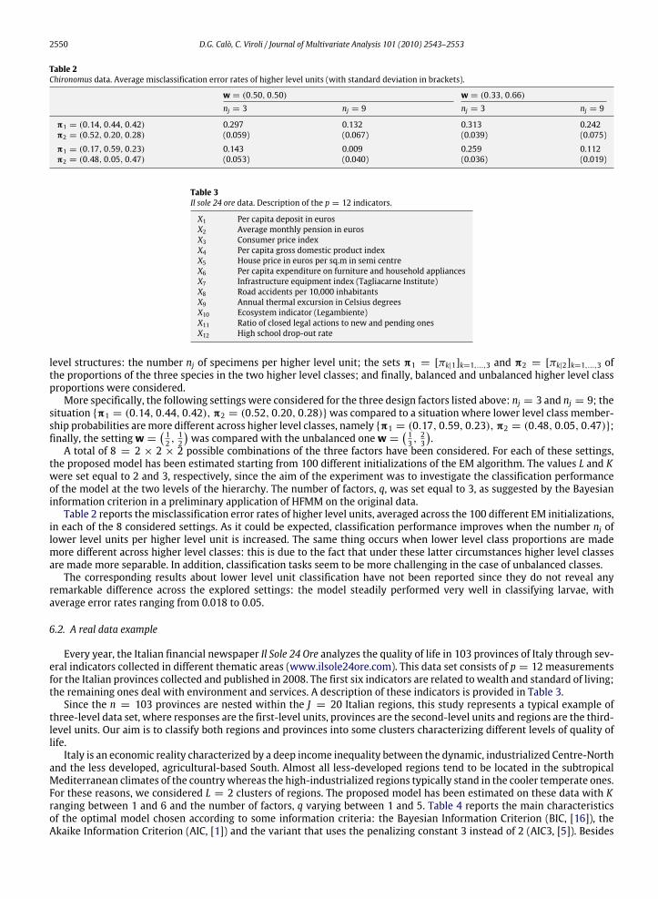
Table 2Chironomus data. Average misclassification error rates of higher level units (with standard deviation in brackets).

w = (0.50, 0.50) w = (0.33, 0.66)nj = 3 nj = 9 nj = 3 nj = 9

π1 = (0.14, 0.44, 0.42) 0.297 0.132 0.313 0.242π2 = (0.52, 0.20, 0.28) (0.059) (0.067) (0.039) (0.075)

π1 = (0.17, 0.59, 0.23) 0.143 0.009 0.259 0.112π2 = (0.48, 0.05, 0.47) (0.053) (0.040) (0.036) (0.019)

Table 3Il sole 24 ore data. Description of the p = 12 indicators.

X1 Per capita deposit in eurosX2 Average monthly pension in eurosX3 Consumer price indexX4 Per capita gross domestic product indexX5 House price in euros per sq.m in semi centreX6 Per capita expenditure on furniture and household appliancesX7 Infrastructure equipment index (Tagliacarne Institute)X8 Road accidents per 10,000 inhabitantsX9 Annual thermal excursion in Celsius degreesX10 Ecosystem indicator (Legambiente)X11 Ratio of closed legal actions to new and pending onesX12 High school drop-out rate

level structures: the number nj of specimens per higher level unit; the sets π1 = [πk|1]k=1,...,3 and π2 = [πk|2]k=1,...,3 ofthe proportions of the three species in the two higher level classes; and finally, balanced and unbalanced higher level classproportions were considered.More specifically, the following settings were considered for the three design factors listed above: nj = 3 and nj = 9; the

situation {π1 = (0.14, 0.44, 0.42),π2 = (0.52, 0.20, 0.28)}was compared to a situation where lower level class member-ship probabilities aremore different across higher level classes, namely {π1 = (0.17, 0.59, 0.23),π2 = (0.48, 0.05, 0.47)};finally, the settingw =

( 12 ,12

)was compared with the unbalanced onew =

( 13 ,23

).

A total of 8 = 2 × 2 × 2 possible combinations of the three factors have been considered. For each of these settings,the proposed model has been estimated starting from 100 different initializations of the EM algorithm. The values L and Kwere set equal to 2 and 3, respectively, since the aim of the experiment was to investigate the classification performanceof the model at the two levels of the hierarchy. The number of factors, q, was set equal to 3, as suggested by the Bayesianinformation criterion in a preliminary application of HFMM on the original data.Table 2 reports the misclassification error rates of higher level units, averaged across the 100 different EM initializations,

in each of the 8 considered settings. As it could be expected, classification performance improves when the number nj oflower level units per higher level unit is increased. The same thing occurs when lower level class proportions are mademore different across higher level classes: this is due to the fact that under these latter circumstances higher level classesare made more separable. In addition, classification tasks seem to be more challenging in the case of unbalanced classes.The corresponding results about lower level unit classification have not been reported since they do not reveal any

remarkable difference across the explored settings: the model steadily performed very well in classifying larvae, withaverage error rates ranging from 0.018 to 0.05.

6.2. A real data example

Every year, the Italian financial newspaper Il Sole 24 Ore analyzes the quality of life in 103 provinces of Italy through sev-eral indicators collected in different thematic areas (www.ilsole24ore.com). This data set consists of p = 12 measurementsfor the Italian provinces collected and published in 2008. The first six indicators are related to wealth and standard of living;the remaining ones deal with environment and services. A description of these indicators is provided in Table 3.Since the n = 103 provinces are nested within the J = 20 Italian regions, this study represents a typical example of

three-level data set, where responses are the first-level units, provinces are the second-level units and regions are the third-level units. Our aim is to classify both regions and provinces into some clusters characterizing different levels of quality oflife.Italy is an economic reality characterized by a deep income inequality between the dynamic, industrialized Centre-North

and the less developed, agricultural-based South. Almost all less-developed regions tend to be located in the subtropicalMediterranean climates of the countrywhereas the high-industrialized regions typically stand in the cooler temperate ones.For these reasons, we considered L = 2 clusters of regions. The proposed model has been estimated on these data with Kranging between 1 and 6 and the number of factors, q varying between 1 and 5. Table 4 reports the main characteristicsof the optimal model chosen according to some information criteria: the Bayesian Information Criterion (BIC, [16]), theAkaike Information Criterion (AIC, [1]) and the variant that uses the penalizing constant 3 instead of 2 (AIC3, [5]). Besides

http://www.ilsole24ore.com


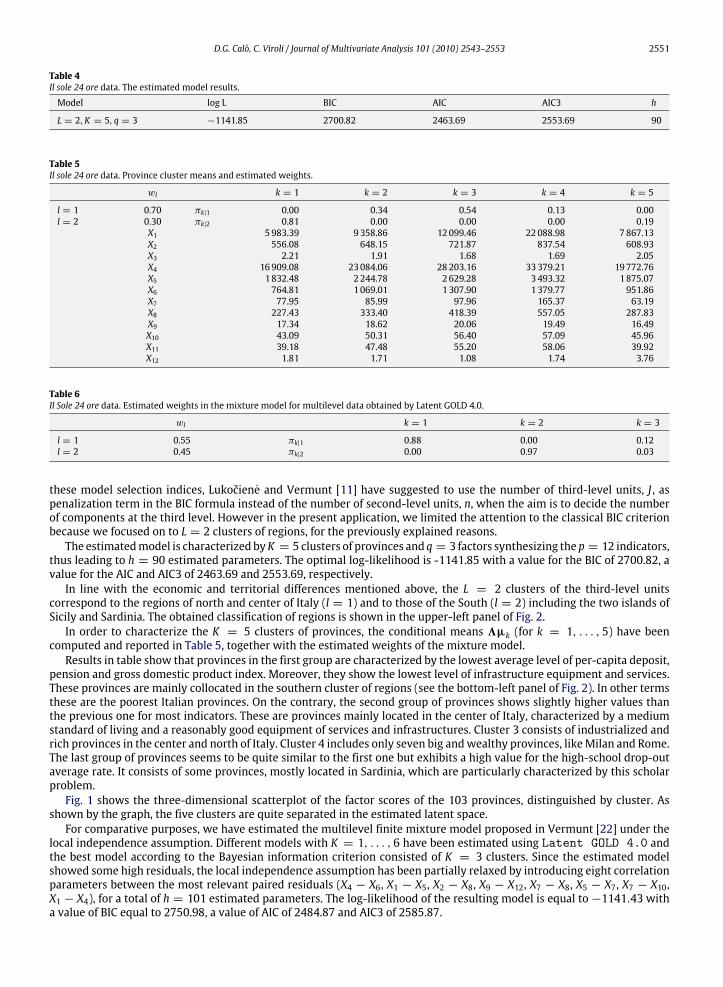
Table 4Il sole 24 ore data. The estimated model results.

Model log L BIC AIC AIC3 h

L = 2, K = 5, q = 3 −1141.85 2700.82 2463.69 2553.69 90

Table 5Il sole 24 ore data. Province cluster means and estimated weights.

wl k = 1 k = 2 k = 3 k = 4 k = 5

l = 1 0.70 πk|1 0.00 0.34 0.54 0.13 0.00l = 2 0.30 πk|2 0.81 0.00 0.00 0.00 0.19

X1 5983.39 9358.86 12099.46 22088.98 7867.13X2 556.08 648.15 721.87 837.54 608.93X3 2.21 1.91 1.68 1.69 2.05X4 16909.08 23084.06 28203.16 33379.21 19772.76X5 1832.48 2244.78 2629.28 3493.32 1875.07X6 764.81 1069.01 1307.90 1379.77 951.86X7 77.95 85.99 97.96 165.37 63.19X8 227.43 333.40 418.39 557.05 287.83X9 17.34 18.62 20.06 19.49 16.49X10 43.09 50.31 56.40 57.09 45.96X11 39.18 47.48 55.20 58.06 39.92X12 1.81 1.71 1.08 1.74 3.76

Table 6Il Sole 24 ore data. Estimated weights in the mixture model for multilevel data obtained by Latent GOLD 4.0.

wl k = 1 k = 2 k = 3

l = 1 0.55 πk|1 0.88 0.00 0.12l = 2 0.45 πk|2 0.00 0.97 0.03

these model selection indices, Lukočiene and Vermunt [11] have suggested to use the number of third-level units, J , aspenalization term in the BIC formula instead of the number of second-level units, n, when the aim is to decide the numberof components at the third level. However in the present application, we limited the attention to the classical BIC criterionbecause we focused on to L = 2 clusters of regions, for the previously explained reasons.The estimatedmodel is characterized byK = 5 clusters of provinces and q = 3 factors synthesizing the p = 12 indicators,

thus leading to h = 90 estimated parameters. The optimal log-likelihood is -1141.85 with a value for the BIC of 2700.82, avalue for the AIC and AIC3 of 2463.69 and 2553.69, respectively.In line with the economic and territorial differences mentioned above, the L = 2 clusters of the third-level units

correspond to the regions of north and center of Italy (l = 1) and to those of the South (l = 2) including the two islands ofSicily and Sardinia. The obtained classification of regions is shown in the upper-left panel of Fig. 2.In order to characterize the K = 5 clusters of provinces, the conditional means 3µk (for k = 1, . . . , 5) have been

computed and reported in Table 5, together with the estimated weights of the mixture model.Results in table show that provinces in the first group are characterized by the lowest average level of per-capita deposit,

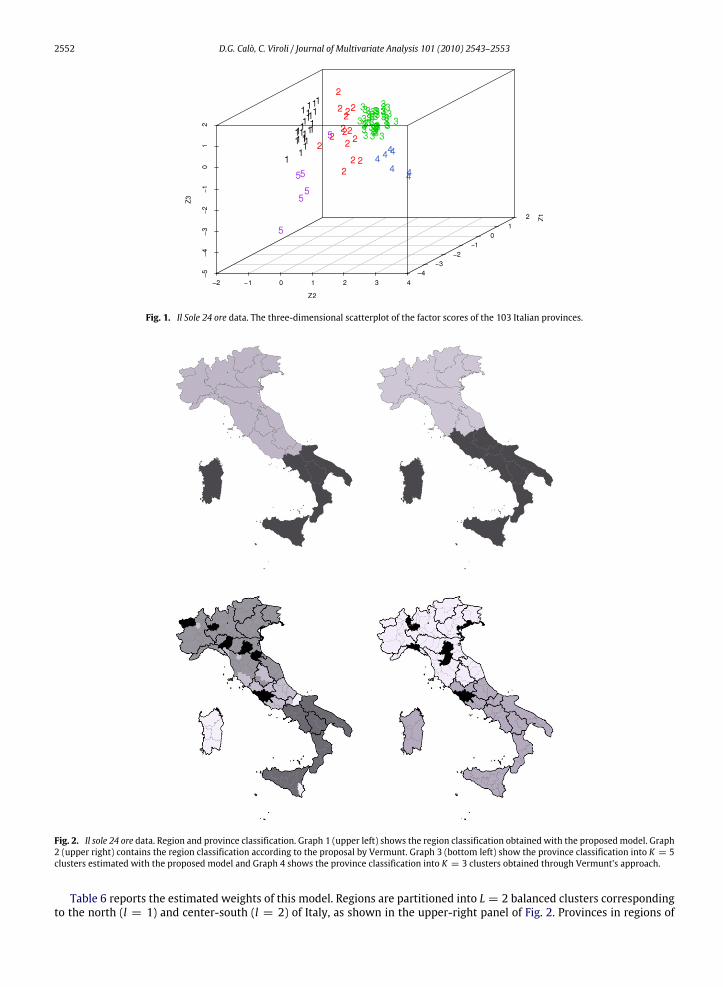
pension and gross domestic product index. Moreover, they show the lowest level of infrastructure equipment and services.These provinces are mainly collocated in the southern cluster of regions (see the bottom-left panel of Fig. 2). In other termsthese are the poorest Italian provinces. On the contrary, the second group of provinces shows slightly higher values thanthe previous one for most indicators. These are provinces mainly located in the center of Italy, characterized by a mediumstandard of living and a reasonably good equipment of services and infrastructures. Cluster 3 consists of industrialized andrich provinces in the center and north of Italy. Cluster 4 includes only seven big andwealthy provinces, likeMilan and Rome.The last group of provinces seems to be quite similar to the first one but exhibits a high value for the high-school drop-outaverage rate. It consists of some provinces, mostly located in Sardinia, which are particularly characterized by this scholarproblem.Fig. 1 shows the three-dimensional scatterplot of the factor scores of the 103 provinces, distinguished by cluster. As

shown by the graph, the five clusters are quite separated in the estimated latent space.For comparative purposes, we have estimated the multilevel finite mixture model proposed in Vermunt [22] under the

local independence assumption. Different models with K = 1, . . . , 6 have been estimated using Latent GOLD 4.0 andthe best model according to the Bayesian information criterion consisted of K = 3 clusters. Since the estimated modelshowed some high residuals, the local independence assumption has been partially relaxed by introducing eight correlationparameters between the most relevant paired residuals (X4 − X6, X1 − X5, X2 − X8, X9 − X12, X7 − X8, X5 − X7, X7 − X10,X1 − X4), for a total of h = 101 estimated parameters. The log-likelihood of the resulting model is equal to−1141.43 witha value of BIC equal to 2750.98, a value of AIC of 2484.87 and AIC3 of 2585.87.


Fig. 1. Il Sole 24 ore data. The three-dimensional scatterplot of the factor scores of the 103 Italian provinces.

Fig. 2. Il sole 24 ore data. Region and province classification. Graph 1 (upper left) shows the region classification obtained with the proposed model. Graph2 (upper right) contains the region classification according to the proposal by Vermunt. Graph 3 (bottom left) show the province classification into K = 5clusters estimated with the proposed model and Graph 4 shows the province classification into K = 3 clusters obtained through Vermunt’s approach.

Table 6 reports the estimated weights of this model. Regions are partitioned into L = 2 balanced clusters correspondingto the north (l = 1) and center-south (l = 2) of Italy, as shown in the upper-right panel of Fig. 2. Provinces in regions of


the Center-South cluster into a whole group which corresponds to the poorest provinces (π2|2 = 0.97). Provinces in thenorth of Italy cluster into two groups, a numerous group of ‘‘middle’’ provinces (π1|1 = 0.88) and a small group of eight bigand important provinces (π1|3 = 0.12) including Rome and Milan. This classification is shown in the bottom-right panel ofFig. 2.

7. Conclusions

In this paper, a model for clustering multilevel data has been introduced by combining tools from different backgrounds.Starting from the recent proposals on latent class analysis formultilevel data, we have defined and explored a dimensionallyreduced solution. It is achieved by introducing a latent factor model in order to reduce the number of free parameters of themixture model, without requiring the local independence assumption. In so doing the trade-off between model parsimonyand flexibility is governed. In the illustrated real example, a meaningful clustering of both second- and third-level unitshas been obtained by estimating a model involving less parameters than those required by traditional multilevel mixturemodeling.From a computational point of view, the proposed model has been estimated using an EM-algorithm. The algorithm did

not show any convergence problemwhen properly initialized.We have implemented it in R code and it is available from theauthors upon request. In addition, we tried fitting the proposed model with the standard software for mixture models. Asfar as Mplus 5 [15] is concerned, the model can be framed in the context of two-level confirmatory factor analysis mixturemodeling with continuous factor indicators; in our experiments some convergence problems have occurred when factorswere allowed to be heteroscedastic. The GUI version of Latent Gold does not allow us to directly specify the model;however, the model could be specified and estimated using the syntax version of the software.

References

[1] H. Akaike, A new look at statistical model identification, IEEE Trans. Automat. Control 19 (1974) 716–723.[2] S.S. Allua, Evaluation of single-and multilevel factor mixture model estimation, PhD thesis, University of Texas at Austin, 2007.[3] T. Asparouhov, B. Muthen, Multilevel mixture models, in: G.R. Hancock, K.M. Samuelsen (Eds.), Advances in Latent Variable Mixture Models,Information Age Publishing Inc., Charlotte, NC, 2008, pp. 27–51.

[4] W.R. Atchley, J. Martin, A Morphometric analyisis of differential sexual dimorphism in larvae of Chironomus, Can. Entomol. 108 (1971) 819–827.[5] H. Bozdogan, Determining the number of component clusters in the standard multivariate normal mixture model using model-selecton criteria,Technical Report No. UIC/DQM/A83-1, Quantitative Methods Department, University of Illinois at Chicago, 1983.

[6] N.M. Dempster, A.P. Laird, D.B. Rubin, Maximum likelihood from incomplete data via the EM algorithm (with discussion), J. R. Stat. Soc. Ser. B Stat.Methodol. 39 (1977) 1–38.

[7] C. Fraley, A.E. Raftery, Model-based clustering, discriminant analysis, and density estimation, J. Amer. Statist. Assoc. 97 (2002) 611–631.[8] C. Fraley, A.E. Raftery, MCLUST Version 3 for R: Normal Mixture Modeling and Model-based Clustering, Technical Report No. 504, Department ofStatistics, University of Washington, 2006.

[9] L.A. Goodman, Exploratory latent structure analysis using both identifiable and unidentifiable models, Biometrika 61 (1974) 215–231.[10] G.H. Lubke, B. Muthén, Investigating population heterogeneity with factor mixture models, Psychol. Methods 10 (2005) 21–39.[11] O. Lukočiene, J.K. Vermunt, Determining the number of components in mixture models for hierarchical data, in: A. Fink, et al. (Eds.), Advances in Data

Analysis, Data Handling and Business Intelligence, Springer, Heidelberg, 2010, pp. 241–249.[12] K.V. Mardia, J.T. Kent, J.M. Bibby, Multivariate Analysis, Academic Press, Oxford, 1976.[13] G.J. McLachlan, D. Peel, Finite Mixture Models, Wiley, New York, 2000.[14] A. Montanari, C. Viroli, Heteroscedastic factor mixture analysis, Stat. Model., 2010 (in press).[15] L.K. Muthén, B.O. Muthén, Mplus Users Guide, fifth ed., Los Angeles, 2007.[16] G. Schwarz, Estimating the dimension of a model, Ann. Statist. 6 (1978) 461–464.[17] A. Skrondal, S. Rabe-Hesketh, Generalized Latent VariableModeling: Multilevel, Longitudinal and Structural EquationModels, Chapmal and Hall, New

York, 2004.[18] A.B. Snijders, R.J. Bosker, Multilevel Analysis, SAGE Publications, London, 1999.[19] J.K. Vermunt, Multilevel latent class models, Sociol. Methodol. 33 (2003) 213–239.[20] J.K. Vermunt, Mixed-effect logistic regression models for indirectly observed outcome variables, Multivariate Behav. Res. 40 (2005) 281–301.[21] J.K. Vermunt, A hierarchical mixture model for clustering three-way data sets, Comput. Statist. Data Anal. 51 (2007) 5368–5376.[22] J.K. Vermunt, Latent class and finite mixture models for multilevel data sets, Stat. Methods Med. Res. 17 (2008) 33–51.[23] J.K. Vermunt, Mixture models for multilevel data sets, in: J. Hox, J.K. Roberts (Eds.), Handbook of Advanced Multilevel Analysis, Lawrence Erlbaum,

2010.[24] J.K. Vermunt, J.Magidson, Hierarchicalmixturemodels for nested data structures, in: C.Weihs,W. Gaul (Eds.), Classification: TheUbiquitous Challenge,

Springer, Heidelberg, 2005, pp. 176–183.[25] J.K. Vermunt, J. Magidson, LG-Syntax User’s Guide: Manual for Latent GOLD 4.5, Syntax Module, Belmont, MA, Statistical Innovations Inc.

A dimensionally reduced finite mixture model for multilevel data

Documents

Transcript of A dimensionally reduced finite mixture model for multilevel data