
Multilevel Hierarchical Modeling of Benthic Macroinvertebrate ...
104
U.S. Department of the Interior U.S. Geological Survey National Water-Quality Assessment Program Scientific Investigations Report 2009–5243 Multilevel Hierarchical Modeling of Benthic Macroinvertebrate Responses to Urbanization in Nine Metropolitan Regions across the Conterminous United States
-
Upload
khangminh22 -
Category
Documents
-
view
0 -
download
0
Transcript of Multilevel Hierarchical Modeling of Benthic Macroinvertebrate ...

U.S. Department of the InteriorU.S. Geological Survey
National Water-Quality Assessment Program
Scientific Investigations Report 2009–5243
Multilevel Hierarchical Modeling of Benthic Macroinvertebrate Responses to Urbanizationin Nine Metropolitan Regions across theConterminous United States

Cover. Background photograph—Rock Creek near Whitsett, North Carolina, a rural stream with relatively little urban influence. Inset photographs—Debris in Pigeon House Branch, a highly urbanized stream in Raleigh, North Carolina; stonefly, a large predatory insect; and water penny, an aquatic beetle larvae (photographs by Michelle Moorman and Eric Sadorf, U.S. Geological Survey).

Multilevel Hierarchical Modeling of Benthic Macroinvertebrate Responses to Urbanization in Nine Metropolitan Regions across the Conterminous United States
By Roxolana Kashuba, YoonKyung Cha, Ibrahim Alameddine, Boknam Lee, and Thomas F. Cuffney
National Water-Quality Assessment Program
Scientific Investigations Report 2009–5243
U.S. Department of the InteriorU.S. Geological Survey

U.S. Department of the InteriorKEN SALAZAR, Secretary
U.S. Geological SurveyMarcia K. McNutt, Director
U.S. Geological Survey, Reston, Virginia: 2010
For more information on the USGS—the Federal source for science about the Earth, its natural and living resources, natural hazards, and the environment, visit http://www.usgs.gov or call 1-888-ASK-USGS
For an overview of USGS information products, including maps, imagery, and publications, visit http://www.usgs.gov/pubprod
To order this and other USGS information products, visit http://store.usgs.gov
Any use of trade, product, or firm names is for descriptive purposes only and does not imply endorsement by the U.S. Government.
Although this report is in the public domain, permission must be secured from the individual copyright owners to reproduce any copyrighted materials contained within this report.
Suggested citation:Kashuba, Roxolana, Cha, YoonKyung, Alameddine, Ibrahim, Lee, Boknam, and Cuffney, T.F., 2010, Multilevel hierarchical modeling of benthic macroinvertebrate responses to urbanization in nine metropolitan regions across the conterminous United States: U.S. Geological Survey Scientific Investigations Report 2009–5243, 88 p.
Available only online at http://pubs.usgs.gov/sir/2009/5243/

iii
Foreword
The U.S. Geological Survey (USGS) is committed to providing the Nation with credible scientific information that helps to enhance and protect the overall quality of life and that facilitates effective management of water, biological, energy, and mineral resources (http://www.usgs.gov/). Information on the Nation’s water resources is critical to ensuring long-term availability of water that is safe for drinking and recreation and is suitable for industry, irrigation, and fish and wildlife. Population growth and increasing demands for water make the availability of that water, measured in terms of quantity and quality, even more essential to the long-term sustain-ability of our communities and ecosystems.
The USGS implemented the National Water-Quality Assessment (NAWQA) Program in 1991 to support national, regional, State, and local information needs and decisions related to water-quality management and policy (http://water.usgs.gov/nawqa). The NAWQA Program is designed to answer: What is the condition of our Nation’s streams and groundwater? How are conditions changing over time? How do natural features and human activities affect the qual-ity of streams and groundwater, and where are those effects most pronounced? By combining information on water chemistry, physical characteristics, stream habitat, and aquatic life, the NAWQA Program aims to provide science-based insights for current and emerging water issues and priorities. From 1991 to 2001, the NAWQA Program completed interdisciplinary assessments and established a baseline understanding of water-quality conditions in 51 of the Nation’s river basins and aquifers, referred to as Study Units (http://water.usgs.gov/nawqa/studyu.html).
National and regional assessments are ongoing in the second decade (2001–2012) of the NAWQA Program as 42 of the 51 Study Units are selectively reassessed. These assessments extend the findings in the Study Units by determining water-quality status and trends at sites that have been consistently monitored for more than a decade, and filling critical gaps in characterizing the quality of surface water and groundwater. For example, increased emphasis has been placed on assessing the quality of source water and finished water associated with many of the Nation’s largest community water systems. During the second decade, NAWQA is addressing five national priority topics that build an understanding of how natural features and human activities affect water quality, and establish links between sources of contaminants, the transport of those contaminants through the hydrologic system, and the potential effects of contaminants on humans and aquatic ecosystems. Included are studies on the fate of agricul-tural chemicals, effects of urbanization on stream ecosystems, bioaccumulation of mercury in stream ecosystems, effects of nutrient enrichment on aquatic ecosystems, and transport of con-taminants to public-supply wells. In addition, national syntheses of information on pesticides, volatile organic compounds (VOCs), nutrients, selected trace elements, and aquatic ecology are continuing.
The USGS aims to disseminate credible, timely, and relevant science information to address practical and effective water-resource management and strategies that protect and restore water quality. We hope this NAWQA publication will provide you with insights and information to meet your needs, and will foster increased citizen awareness and involvement in the protec-tion and restoration of our Nation’s waters.

iv
The USGS recognizes that a national assessment by a single program cannot address all water-resource issues of interest. External coordination at all levels is critical for cost-effective man-agement, regulation, and conservation of our Nation’s water resources. The NAWQA Program, therefore, depends on advice and information from other agencies—Federal, State, regional, interstate, Tribal, and local—as well as nongovernmental organizations, industry, academia, and other stakeholder groups. Your assistance and suggestions are greatly appreciated.
Matthew C. Larsen Associate Director for Water

v
ContentsForeword ........................................................................................................................................................iiiAbstract ...........................................................................................................................................................1Introduction.....................................................................................................................................................1
Purpose and Scope ..............................................................................................................................2Methods...........................................................................................................................................................3
Data Collection ......................................................................................................................................4Benthic Macroinvertebrate Data ..............................................................................................4Land-Cover Data ..........................................................................................................................4Climate Data..................................................................................................................................4
Data Summary .......................................................................................................................................5Urbanization Measures ..............................................................................................................5Macroinvertebrate Response Variables ..................................................................................5Land-Cover Types ........................................................................................................................9Scale-Dependent Variables .....................................................................................................11
Basin Scale ........................................................................................................................11Regional Scale ..................................................................................................................13
Technique: Multilevel Hierarchical Models ...................................................................................14Model Structure .........................................................................................................................18Model Fitting ...............................................................................................................................21Model Limitations.......................................................................................................................23
Predicting and Understanding Effects of Urbanization .........................................................................24Preliminary Land Cover Analysis .....................................................................................................24Model Summary (Model Results) .....................................................................................................29
Model 1: No Region-Level Predictor ......................................................................................30Model 2: PRECIP Region-Level Predictor ..............................................................................38Model 3: TEMP Region-Level Predictor .................................................................................43Model 4: PRECIP and TEMP Region-Level Predictors .........................................................46Model 5: AG (Continuous) Region-Level Predictor ..............................................................49Model 6: AG (Categorical) and PRECIP Region-Level Predictors ......................................52Model 7: AG (Categorical) and TEMP Region-Level Predictors ........................................58Model 8: AG (Categorical), PRECIP, and TEMP Region-Level Predictors .........................62
Model Interpretation ..........................................................................................................................62Effect of Precipitation ...............................................................................................................62Effect of Temperature ................................................................................................................65Effect of Antecedent Agriculture ............................................................................................66
Conclusions...................................................................................................................................................66General Ecological Trends ................................................................................................................66Utility of Modeling Methodology ......................................................................................................67Measures of Model Fit .......................................................................................................................67Variable Limitations ............................................................................................................................67Future Directions.................................................................................................................................69
Acknowledgments .......................................................................................................................................69References ....................................................................................................................................................69Appendix........................................................................................................................................................74

vi
Figures 1. Map showing locations of the nine metropolitan regions for which benthic
macroinvertebrate responses to urbanization were modeled ..............................................2 2. Box plots of urbanization measures ..........................................................................................6 3. Histograms and scatterplots of urbanization measures ........................................................7 4. Box plots of macroinvertebrate response variables ..............................................................8 5. Histograms and scatterplots of macroinvertebrate response variables ..........................10 6. Box plot of the percentage of current agriculture (NLCD7 and NLCD8)
in each region ..............................................................................................................................11 7. Estimates of the percentage of antecedent agriculture (AG) in each region ..................12 8. Box plot of drainage basin area in each region ....................................................................13 9. Box plots of mean annual precipitation and mean annual ambient temperature
for the period from 1980 to 1997 in each region ....................................................................13 10. Multilevel hierarchical modeling framework without group-level predictors .................15 11. Multilevel hierarchical modeling framework with group-level predictors .......................17 12. Scatterplots of the percentage of agriculture (NLCD7 and NLCD8) compared to the
percentage of forest (NLCD4 and NLCD5) for each region .................................................26 13. Scatterplots of the percentage of urban (NLCD2) compared to the percentage
of agriculture (NLCD7 and NLCD8) for each region ..............................................................27 14. Scatterplots of the percentage of agriculture (NLCD7 and NLCD8) compared to
macroinvertebrate response variables (NMDS1, RICH, EPTRICH, and RICHTOL) for agriculture-dominant regions .............................................................................................28
15. Scatterplots of NMDS1 compared to URB for each region with complete pooling, no pooling, and Model 1: No region-level predictors ...........................................................31
16. Scatterplots of RICH compared to URB for each region with complete pooling, no pooling, and Model 1: No region-level predictors ...........................................................33
17. Scatterplots of EPTRICH compared to URB for each region with complete pooling, no pooling, and Model 1: No region-level predictors ...........................................................35
18. Scatterplots of RICHTOL compared to URB for each region with complete pooling, no pooling, and Model 1: No region-level predictors ...........................................................37
19. NMDS1 multilevel hierarchical Model 2: Region-level precipitation predictor for intercept and slope ...............................................................................................................39
20. RICH multilevel hierarchical Model 2: Region-level precipitation predictor for intercept and slope ...............................................................................................................40
21. EPTRICH multilevel hierarchical Model 2: Region-level precipitation predictor for intercept and slope ...............................................................................................................41
22. RICHTOL multilevel hierarchical Model 2: Region-level precipitation predictor for intercept and slope ...............................................................................................................42
23. NMDS1 multilevel hierarchical Model 3: Region-level temperature predictor for intercept and slope ...............................................................................................................43
24. RICH multilevel hierarchical Model 3: Region-level temperature predictor for intercept and slope ...............................................................................................................44
25. EPTRICH multilevel hierarchical Model 3: Region-level temperature predictor for intercept and slope ...............................................................................................................45
26. RICHTOL multilevel hierarchical Model 3: Region-level temperature predictor for intercept and slope ...............................................................................................................45

vii
27. NMDS1 multilevel hierarchical Model 4: Region-level temperature predictor for intercept and region-level precipitation predictor for slope .........................................47
28. RICH multilevel hierarchical Model 4: Region-level temperature predictor for intercept and region-level precipitation predictor for slope .........................................47
29. EPTRICH multilevel hierarchical Model 4: Region-level temperature predictor for intercept and region-level precipitation predictor for slope .........................................48
30. RICHTOL multilevel hierarchical Model 4: Region-level temperature predictor for intercept and region-level precipitation predictor for slope .........................................48
31. NMDS1 multilevel hierarchical Model 5: Region-level antecedent agriculture percent predictor for intercept and slope ..............................................................................50
32. RICH multilevel hierarchical Model 5: Region-level antecedent agriculture percent predictor for intercept and slope ..............................................................................50
33. EPTRICH multilevel hierarchical Model 5: Region-level antecedent agriculture percent predictor for intercept and slope ..............................................................................51
34. RICHTOL multilevel hierarchical Model 5: Region-level antecedent agriculture percent predictor for intercept and slope ..............................................................................51
35. NMDS1 multilevel hierarchical Model 6: Region-level precipitation and categorical antecedent agriculture predictors for intercept and slope .................................................53
36. RICH multilevel hierarchical Model 6: Region-level precipitation and categorical antecedent agriculture predictors for intercept and slope .................................................53
37. EPTRICH multilevel hierarchical Model 6: Region-level precipitation and categorical antecedent agriculture predictors for intercept and slope .................................................54
38. RICHTOL multilevel hierarchical Model 6: Region-level precipitation and categorical antecedent agriculture predictors for intercept and slope .................................................54
39. NMDS1 multilevel hierarchical Model 7: Region-level temperature and categorical antecedent agriculture predictors for intercept and slope .................................................59
40. RICH multilevel hierarchical Model 7: Region-level temperature and categorical antecedent agriculture predictors for intercept and slope .................................................59
41. EPTRICH multilevel hierarchical Model 7: Region-level temperature and categorical antecedent agriculture predictors for intercept and slope .................................................60
42. RICHTOL multilevel hierarchical Model 7: Region-level temperature and categorical antecedent agriculture predictors for intercept and slope .................................................60
43. NMDS1 multilevel hierarchical Model 8: Region-level temperature and categorical antecedent agriculture predictors for intercept and region-level precipitation and categorical antecedent agriculture predictors for slope ....................................................63
44. RICH multilevel hierarchical Model 8: Region-level temperature and categorical antecedent agriculture predictors for intercept and region-level precipitation and categorical antecedent agriculture predictors for slope ....................................................63
45. EPTRICH multilevel hierarchical Model 8: Region-level temperature and categorical antecedent agriculture predictors for intercept and region-level precipitation and categorical antecedent agriculture predictors for slope ....................................................64
46. RICHTOL multilevel hierarchical Model 8: Region-level temperature and categorical antecedent agriculture predictors for intercept and region-level precipitation and categorical antecedent agriculture predictors for slope ....................................................64

viii
Tables 1. Major environmental characteristics of the nine metropolitan regions .............................3 2. Spearman rank correlation coefficients for urbanization measures ...................................7 3. Spearman rank correlation coefficients for macroinvertebrate response variables .....10 4. Antecedent agriculture (AG) of each region for non-urbanized basins ............................12 5. Delineation of variables included in the eight multilevel hierarchical models
per response variable ................................................................................................................18 6. Summary of unpooled regressions between URB and invertebrate response
variables based on 243 equivalent degrees of freedom ......................................................24 7. Summary of regressions between percentage of agriculture land-cover
(NLDC7 and NLDC8) and invertebrate response variables based on 243 equivalent degrees of freedom ....................................................................................................................25
8. Deviance information criteria (DIC) for the eight different multilevel hierarchical models per response variable ..................................................................................................29
9. Intercept and slope coefficient estimates, representing background condition prior to urbanization and rate of change with urbanization, respectively, and variance coef-ficient estimates for invertebrate response NMDS1 Model 1, unpooled model, and completely pooled model ...................................................................................................30
10. Intercept and slope coefficient estimates, representing background condition prior to urbanization and rate of change with urbanization, respectively, and variance coef-ficient estimates for invertebrate response RICH Model 1, unpooled model, and completely pooled model ...................................................................................................32
11. Intercept and slope coefficient estimates, representing background condition prior to urbanization and rate of change with urbanization, respectively, and variance coef-ficient estimates for invertebrate response EPTRICH Model 1, unpooled model, and completely pooled model ..........................................................................................................34
12. Intercept and slope coefficient estimates, representing background condition prior to urbanization and rate of change with urbanization, respectively, and variance coef-ficient estimates for invertebrate response RICHTOL Model 1, unpooled model, and completely pooled model ..........................................................................................................36
13. Regional intercept and slope coefficient estimates, representing regional background condition prior to urbanization and regional rate of change with urbanization, respectively, hyperparameter intercept and slope coefficient estimates and variance coefficient estimates for invertebrate response NMDS1 Models 2–5 ......39
14. Regional intercept and slope coefficient estimates, representing regional background condition prior to urbanization and regional rate of change with urbanization, respectively, hyperparameter intercept and slope coefficient estimates and variance coefficient estimates for invertebrate response RICH Models 2–5 ...........40
15. Regional intercept and slope coefficient estimates, representing regional background condition prior to urbanization and regional rate of change with urbanization, respectively, hyperparameter intercept and slope coefficient estimates and variance coefficient estimates for invertebrate response EPTRICH Models 2–5 ....41
16. Regional intercept and slope coefficient estimates, representing regional background condition prior to urbanization and regional rate of change with urbanization, respectively, hyperparameter intercept and slope coefficient estimates and variance coefficient estimates for invertebrate response RICHTOL Models 2–5 ...................................................................................................................................42

ix
17. Regional intercept and slope coefficient estimates, representing regional background condition prior to urbanization and regional rate of change with urbanization, respectively, hyperparameter intercept and slope coefficient estimates and variance coefficient estimates for invertebrate response NMDS1 Models 6–8 ......55
18. Regional intercept and slope coefficient estimates, representing regional background condition prior to urbanization and regional rate of change with urbanization, respectively, hyperparameter intercept and slope coefficient estimates and variance coefficient estimates for invertebrate response EPTRICH Models 6–8 ....56
19. Regional intercept and slope coefficient estimates, representing regional background condition prior to urbanization and regional rate of change with urbanization, respectively, hyperparameter intercept and slope coefficient estimates and variance coefficient estimates for invertebrate response RICH Models 6–8 ...........57
20. Regional intercept and slope coefficient estimates, representing regional background condition prior to urbanization and regional rate of change with urbanization, respectively, hyperparameter intercept and slope coefficient estimates and variance coefficient estimates for invertebrate response RICHTOL Models 6–8 ....61
Conversion Factors, Acronyms, Abbreviations, and Definitions
Multiply By To obtain
Lengthmeter (m) 3.281 foot (ft) kilometer (km) 0.6214 mile (mi)kilometer (km) 0.5400 mile, nautical (nmi) meter (m) 1.094 yard (yd)
Areasquare meter (m2) 0.0002471 acre square kilometer (km2) 247.1 acresquare meter (m2) 10.76 square foot (ft2) hectare (ha) 0.003861 square mile (mi2) square kilometer (km2) 0.3861 square mile (mi2)
Vertical coordinate information is referenced to the North American Vertical Datum of 1988 (NAVD 88).
Horizontal coordinate information is referenced to the North American Datum of 1983 (NAD 83).
Elevation, as used in this report, refers to distance above the vertical datum.

x
Metropolitan region abbreviationsATL Atlanta, GA, metropolitan regionBIR Birmingham, AL, metropolitan regionBOS Boston, MA, metropolitan regionDEN Denver, CO, metropolitan regionDFW Dallas-Fort Worth, TX, metropolitan regionMGB Milwaukee-Green Bay, WI, metropolitan regionPOR Portland, OR, metropolitan regionRAL Raleigh, NC, metropolitan regionSLC Salt Lake City, UT, metropolitan region
DefinitionsAG Antecedent agriculture DIC Deviance Information CriterionDPAC-Ck Distributing ambiguous parents among childrenECO Desired basin-level ecological response variable in R code terminologyEPT Ephemeroptera, Plecoptera, and Trichoptera ordersEPTRICH Combined richness of Ephemeroptera, Plecoptera, and Trichoptera ordersEUSE Effects of Urbanization on Stream Ecosystems studiesGIS Geographic Information Systemglmer Generalized linear mixed-effect model R functionHU Housing unit densityIDAS USGS Invertebrate Data Analysis SystemIS Percentage impervious surface areaLCL Lower 95% confidence limitlmer Linear mixed-effect model R functionMA-NUII Metropolitan area national urban intensity indexMA-UII Metropolitan area urban intensity indexMCMC Markov Chain Monte CarloN Number of sample basinsNAWQA National Water-Quality Assessment ProgramNLCD01 National Land Cover Data 2001NLCD1 National Land Cover Data class 1: waterNLCD2 National Land Cover Data class 2: urbanNLCD3 National Land Cover Data class 3: barrenNLCD4 National Land Cover Data class 4: forestNLCD5 National Land Cover Data class 5: shrubsNLCD7 National Land Cover Data class 7: grasslandsNLCD8 National Land Cover Data class 8: crop and pasture landsNLCD9 National Land Cover Data class 9: wetlandsNMDS1 Nonmetric multidimensional scaling first axis ordination basin scoresNOAA National Oceanic and Atmospheric AdministrationNUII National urban intensity indexPOP Population densityPRECIP Mean annual precipitationr Spearman rank correlation coefficientR R statistical software programRD Road densityRICH Total taxa richnessRICHTOL Richness-weighted mean tolerance of taxa at a basinRPKC-C Deleting ambiguous parentsRTH Richest targeted habitatTEMP Mean annual air temperatureUCL Upper 95% confidence limitURB Percentage of basin area in developed land

xi
USGS U.S. Geological Survey≥ Greater than or equal to≤ Less than or equal to> Greater than< Less than% Percentagei Individual sample indexj Region index (j=1 through 9 regions)k AG group index (k=0 for low AG, k=1 for high AG)
αj Estimated intercept for Region j (the estimated invertebrate response at URB=0)
βjEstimated slope for Region j (the estimated change in invertebrate response
per unit change in URB)
µα Mean of region-level intercepts
µβ Mean of region-level slopes
Within-region variance in invertebrate response
Between-region variance in intercept
Between-region variance in slope
γα0 Hyperparameter intercept predicting region-level intercepts
γα1 Hyperparameter slope predicting region-level intercepts
γβ0 Hyperparameter intercept predicting region-level slopes
γβ1 Hyperparameter slope predicting region-level slopes
δαk=1 Effect of high AG on region-level intercept
δαk=0 Effect of low AG on region-level intercept
δβk=1 Effect of high AG on region-level slope
δβk=0 Effect of low AG on region-level slope
δαj Effect of region on region-level intercept
δβj Effect of region on region-level slope
ρ Correlation of model coefficients, αj and βjρj Correlation of model coefficients δαj and δβjρk Correlation of model coefficients δαk and δβk
2y22


AbstractMultilevel hierarchical modeling methodology has been
developed for use in ecological data analysis. The effect of urbanization on stream macroinvertebrate communities was measured across a gradient of basins in each of nine metropolitan regions across the conterminous United States. The hierarchical nature of this dataset was harnessed in a multi-tiered model structure, predicting both invertebrate response at the basin scale and differences in invertebrate response at the region scale. Ordination site scores, total taxa richness, Ephemeroptera, Plecoptera, Trichoptera (EPT) taxa richness, and richness-weighted mean tolerance of organisms at a site were used to describe invertebrate responses. Percent-age of urban land cover was used as a basin-level predictor variable. Regional mean precipitation, air temperature, and antecedent agriculture were used as region-level predictor variables. Multilevel hierarchical models were fit to both levels of data simultaneously, borrowing statistical strength from the complete dataset to reduce uncertainty in regional coefficient estimates. Additionally, whereas non-hierarchical regressions were only able to show differing relations between invertebrate responses and urban intensity separately for each region, the multilevel hierarchical regressions were able to explain and quantify those differences within a single model. In this way, this modeling approach directly establishes the importance of antecedent agricultural conditions in masking the response of invertebrates to urbanization in metropolitan regions such as Milwaukee–Green Bay, Wisconsin; Denver, Colorado; and Dallas–Fort Worth, Texas. Also, these models show that regions with high precipitation, such as Atlanta, Georgia; Birmingham, Alabama; and Portland, Oregon, start out with better regional background conditions of
invertebrates prior to urbanization but experience faster negative rates of change with urbanization. Ultimately, this urbanization-invertebrate response example is used to detail the multilevel hierarchical construction methodology, showing how the result is a set of models that are both statistically more rigorous and ecologically more interpretable than simple linear regression models.
IntroductionStream ecosystems are increasingly affected by urban
development associated with human population growth (Booth and Jackson, 1997; Paul and Meyer, 2001; Walsh and others, 2001; Tate and others, 2005; Walsh and others, 2005). Deforestation destroys riparian buffer zones and leads to declines in canopy cover, changes in energy inputs, and increases in water temperatures (Waite and Carpenter, 2000; Jacobson, 2001; Sprague and others, 2006). Residential and industrial development introduces human waste, pesticides, and industrial chemicals into the water and sediment (Hall and Anderson, 1988; Pitt and others, 1995; Van Metre and others, 2000; Mahler and others, 2005; Gilliom and others, 2006). Impervious surfaces reduce rainfall infiltration, increase surface runoff, and alter the frequency and magnitude of peak and base flows (Klein, 1979; Poff and others, 1997; U.S. Environmental Protection Agency, 1997; Finkenbine and others, 2000; Konrad and Booth, 2002; McMahon and others, 2003; Roy and others, 2005). Altering the hydrology changes channel morphology, degrades aquatic habitats (Winterbourn and Townsend, 1991), and increases sedimentation rates (Wolman and Schick, 1967; Trimble, 1997; Sponseller and others, 2001; Roy and others, 2003b). Changes in land cover, hydrology, and impervious surface also affect stream tempera-ture (Sinokrot and Stefan, 1993; LeBlanc and others, 1997; Paul and Meyer, 2001). Collectively, these and other changes in the physical and chemical environment have been associ-ated with degraded invertebrate assemblages in many urban
Multilevel Hierarchical Modeling of Benthic Macroinvertebrate Responses to Urbanization in Nine Metropolitan Regions across the Conterminous United States
By Roxolana Kashuba,1 YoonKyung Cha,1 Ibrahim Alameddine,1 Boknam Lee,1 and Thomas F. Cuffney2
1 Nicholas School of the Environment, Duke University, Box 90328, Durham, North Carolina 27708.
2 U.S. Geological Survey, North Carolina Water Science Center, 3916 Sunset Ridge Road, Raleigh, North Carolina 27607.

2 Multilevel Hierarchical Modeling of Benthic Macroinvertebrates to Urbanization in Nine Metropolitan Regions
areas (Klein, 1979; Jones and Clark, 1987; Schueler and Galli, 1992; Lenat and Crawford, 1994; Yoder and Rankin, 1996; Horner and others, 1997; Kemp and Spotila, 1997; Kennen, 1999; Yoder and others, 1999; Beasley and Kneale, 2002; Huryn and others, 2002; Kennen and Ayers, 2002; Morley and Karr, 2002; Morse and others, 2003; Ourso and Frenzel, 2003; Roy and others, 2003a; Vølstad and others, 2003; Fitzpatrick and others, 2004; Brown and Vivas, 2005).
In 1999, the U.S. Geological Survey (USGS) initiated a series of urban stream studies (Effects of Urbanization on Stream Ecosystems, EUSE) as part of the National Water-Quality Assessment (NAWQA) Program. The EUSE studies are based on a common study design (McMahon and Cuffney, 2000; Coles and others, 2004; Cuffney and others, 2005; Tate and others, 2005) and consistent measures of urban intensity (Cuffney and Falcone, 2008) and sample-collection and processing methods (Fitzpatrick and others, 1998; Moulton and others, 2002). Nine major metropolitan regions—Boston, MA (BOS); Raleigh, NC (RAL); Atlanta, GA (ATL); Birming-ham, AL (BIR); Milwaukee–Green Bay, WI (MGB); Denver, CO (DEN); Dallas–Fort Worth, TX (DFW); Salt Lake City, UT (SLC); and Portland, OR (POR) (fig. 1)—were chosen to represent the effects of urbanization in regions of the country that differ in potential natural vegetation, air temperature, precipitation, basin relief, elevation, and basin slope (table 1). Each metropolitan region represents a geographically exten-sive region that includes numerous cities and towns in addition to the one for which it is named. EUSE studies have been used to describe the effects of urbanization on fish (Brown and others, 2009), benthic macroinvertebrates (Cuffney and others, in press), algae (Coles and others, 2009), habitat (Faith A. Fitzpatrick, U.S. Geological Survey, written commun., 2009), and water chemistry (Sprague and others, 2007).
Purpose and Scope
The purpose of this report is to develop and document an innovative multilevel hierarchical modeling framework that can be used to describe the response of benthic macroinverte-brates to urbanization (percentage of basin area in developed land, URB) and climatic factors (precipitation and air temperature) within and across the nine metropolitan regions that are included in the EUSE studies. The scope of benthic invertebrate response is limited to four assemblage metrics: nonmetric multidimensional scaling first axis ordination basin scores (NMDS1), total taxa richness (RICH), combined richness of Ephemeroptera, Plecoptera, and Trichoptera (EPTRICH), and richness-weighted mean tolerance of taxa at a basin (RICHTOL). The derivation of the models developed in this study involves:1. Description and analysis of the selected response vari-
ables along with the considered predictor variables,
2. Description of the methodology used to develop and assess the multilevel hierarchical models linking inverte-brate assemblage responses to URB, precipitation, and air temperature,
3. Development of multilevel hierarchical models that combine both local (basin) and regional variables within the model structure to predict the response of invertebrate assemblages to increased urbanization,
4. Assessment of interactions between urbanization, climate, and the condition of stream benthic invertebrate assemblages,
Figure 1. Locations of the nine metropolitan regions for which benthic macroinvertebrate responses to urbanization were modeled. [White circles indicate East regions; black circles indicate Central regions (high antecedent agriculture); white diamonds indicate West regions]

Methods 3
5. Comparison of the results generated by the different models and the metrics used to characterize invertebrate responses, and
6. Identification of the main constraints associated with the modeling methodology, selected computational execution techniques, and model formulation.
The multilevel hierarchical models described in this report link invertebrate responses to urbanization and impor-tant climate parameters (precipitation and air temperature) within each metropolitan region while simultaneously explain-ing differences in the rates at which invertebrate assemblages respond to urbanization across the nine metropolitan regions. These models, in combination with the four invertebrate response metrics, are used to identify appropriate predictor variables and invertebrate metrics for describing changes in the condition of the invertebrate assemblages. Demonstration of the utility of the multilevel hierarchical models will serve as a template for modeling the response of other biological indi-cators (fish and algal assemblages) to increased urbanization.
This report does not incorporate a thorough analysis of all possible region-level influences. The selection of invertebrate response and environmental variables was guided by previous analysis (Cuffney and others, in press). Of all EUSE data col-lected, it is possible that there are other region-level variables (such as chemical concentrations, elevations, and many more) that account for differences between regions in intercept and slope. The focus of this report project is the development of analytical statistical methodology and does not incorporate a thorough scientific analysis to determine all possible factors at which scales affect species composition, abundance, and richness in stream ecosystems. The ecological community effects predicted from urbanization indicators are broad and hard to generalize. Because there are many different species of macroinvertebrates, all potentially affected by different influences, finding predictor variables that apply to the entire
aquatic assemblage is challenging. The goal of this research effort is to introduce a new way of looking at urbanization-effects modeling data, to explain why this modeling approach makes sense in this context, to show exactly how to fit these types of models (including providing R code in the Appendix), and to demonstrate how to interpret the results ecologically. Ultimately, the multilevel hierarchical models can be used to describe and quantify ecologically relevant relations and can become a useful tool for ecological data analysis and interpretation.
Methods
The nine urban studies were conducted using a common study design (McMahon and Cuffney 2000; Coles and others 2004; Cuffney and others 2005; Tate and others 2005) that used nationally available Geographic Information System (GIS) variables (Falcone and others 2007) to define a popula-tion of candidate basins (typically basins drained by second to third order streams) from which 28–30 basins were selected to represent a gradient of urbanization within each region. Local and national GIS variables that represented the natural environmental setting (for example, ecoregion, climate, elevation, stream size) were used to minimize the effects of environmental variability by dividing candidate basins into groups with relatively homogenous environmental features. Urban intensity was defined for each candidate basin by com-bining housing density, percentage of basin area in developed land cover, and road density into an index (metropolitan area national urban intensity index, MA-NUII) scaled to range from 0 (little or no urban) to 100 (maximum urban) within each metropolitan region (Cuffney and Falcone, 2008). Once groups of basins with relatively homogeneous environmental features were defined, 28–30 basins were selected to represent the gradient of urbanization in each metropolitan region.
Table 1. Major environmental characteristics of the nine metropolitan regions.
[%, percentage; °C, degrees Celsius; cm, centimeter; MA-NUII, metropolitan area national urban intensity index]
Metropolitan regionAntecedent
agricultural land covera (%)
Mean annual air temperature
(°C)
Mean annual precipitation
(cm)
Number of candidate
basins
Number of basins in EUSE study
Atlanta, GA (ATL) 17.4 16.3 133.5 116 30Birmingham, AL (BIR) 15.0 16.0 146.8 854 28Boston, MA (BOS) 10.3 8.7 123.2 76 30Denver, CO (DEN) 88.0 9.2 43 204 28Dallas–Fort Worth, TX (DFW) 81.7 18.3 104.2 166 28Milwaukee–Green Bay, WI (MGB) 79.4 7.6 85.5 56 30Portland, OR (POR) 16.9 10.8 152.8 148 28Raleigh, NC (RAL) 24.4 14.9 119.2 871 30Salt Lake City, UT (SLC) 12.2 9.7 68 9 30
a Antecedent agricultural land cover combines row crop and grazing lands at candidate basins with MA-NUII ≤ 10.

4 Multilevel Hierarchical Modeling of Benthic Macroinvertebrates to Urbanization in Nine Metropolitan Regions
This spatially distributed sampling network was intended to represent changes in urbanization through time (that is, substitute space for time).
Conditions in each basin were verified by field reconnais-sance. If conditions in a basin deviated substantially from what was expected, based on the GIS data (for example, substantial new development that was not present on the GIS coverage), or if a sampling reach (150-meter [m] stream section at the outflow of the basin) was disturbed by local-scale effects (for example, channelization, road or building construction), an alternate basin from the same group or a group with similar natural environmental characteristics was selected to represent the same level of urban intensity. The BOS, BIR, and SLC metropolitan regions were studied during 1999–2000; ATL, DEN, and RAL were studied during 2002–2003; and DFW, MGB, and POR were studied during 2003–2004. Details of the study designs are discussed in Coles and others (2004), Cuffney and others (2005), and Tate and others (2005).
The SLC design differed from the other metropolitan regions in that many of the basins were nested, one within another. This modification was necessary because of the small number of streams that are present in SLC and was only possible because urban development in the SLC basins has progressed upstream over time, which ensures that urban intensity increases downstream. The SLC landscape character-izations were restricted to the portions of the basins that were located in the Central Basin and Range ecoregion (Omernik, 1987). Portions in the Wasatch and Uinta Mountains ecoregion were excluded because no urban development has occurred in this area, and the biology and geomorphology of the streams in this ecoregion are different from the Central Basin and Range ecoregion. Large reservoirs in DEN constituted major discontinuities that effectively isolated the upper and lower portions of many of the candidate basins. Consequently, landscape characterizations in DEN were restricted to the portions of the basins that were below the major reservoirs.
Data Collection
All data used in this modeling effort were collected as part of the EUSE studies. Of all measured EUSE variables, this report specifically includes analysis of only benthic macroinvertebrate data, land-cover data, and climate data.
Benthic Macroinvertebrate DataThe NAWQA Program sampling protocols were used to
collect benthic macroinvertebrates over a 1–4 week period during summer low base flows (Cuffney and others [1993] was used for BOS, BIR, and SLC; Moulton and others [2002] was used for ATL, DEN, DFW, MGB, POR, and RAL). Five quantitative richest targeted habitat (RTH) samples were collected from five riffles in each sampling reach using a Slack Sampler (1.25 square meters [m2] total area sampled) except in ATL, DFW, and one SLC basin (Kays Creek at Layton,
UT) where woody snags were sampled (1.4 m2 mean snag area sampled) because riffles were not available. Samples were preserved in 10-percent buffered formalin and sent to the USGS National Water Quality Laboratory in Denver, CO, for taxa identification and enumeration (Moulton and others, 2000). The USGS Invertebrate Data Analysis System (IDAS; Cuffney, 2003) was used to resolve taxonomic ambiguities and calculate assemblage metrics and diversity measures. Ambigu-ous taxa (Cuffney, 2003) were resolved independently for each metropolitan region by distributing ambiguous parents among children (DPAC-Ck) for quantitative samples and deleting ambiguous parents (RPKC-C) for qualitative samples. These options have been shown to be suitable for analyzing responses along urban gradients (Cuffney and others, 2007). Invertebrate attribute data (tolerances and functional groups) were optimized for four regions of the country—mid-Atlantic (BOS), southeast (ATL, BIR, RAL, DFW), midwest (MGB), and northwest (DEN, SLC, POR) on the basis of the attributes compiled by Cuffney (2003). Quantitative richest targeted habitat data (RTH) were converted to densities (number per square meter) prior to resolving ambiguous taxa and calculat-ing assemblage metrics.
Land-Cover DataLand-cover data for ATL, BOS, BIR, RAL, and SLC
were based on the National Land Cover Data 2001 (NLCD01) dataset (U.S. Geological Survey, 2005). Land-cover data for POR were derived (Falcone and others, 2007) by using the NLCD01 class structure to process data from the National Oceanic and Atmospheric Administration (NOAA) Coastal Change Analysis Program (National Oceanic and Atmospheric Administration, 2005). NOAA land-cover classes were recoded to match the NLCD01 classes. Land-cover data for DEN, DFW, and MGB were derived using identical methods and protocols as the NLCD01 program (Falcone and Pearson, 2006). The 16 NLCD01 land-cover classes (U.S. Geological Survey, 2005) were aggregated into eight Anderson Level I classes. For example, “deciduous forest,” “evergreen forest,” and “mixed forest” were aggregated into “forest” (Anderson and others, 1976) because the broader Level I classes were deemed to be more reliable than the Level II classes (Falcone and others, 2007).
Climate DataMean monthly precipitation (in centimeters) and air
temperature (in degrees Celsius) were derived for each of the candidate drainage basins on the basis of 1-kilometer (km) resolution (Daymet, 2005) model data. These data represented 18-year (1980–1997) temperature and precipitation means obtained from terrain-adjusted daily climatological observa-tions (Falcone and others, 2007). Region-level mean annual temperature and mean annual precipitation were obtained by averaging the annual temperature and annual precipitation for the candidate basins in each metropolitan region.

Methods 5
Data Summary
The dataset for the EUSE studies includes variables that characterize the biological, chemical, and physical conditions of 261 basins located in nine metropolitan regions. In this section, the variables that were analyzed are discussed, including six urbanization indicators that delineate census and infrastructure, four assemblage metrics of benthic macroinvertebrates, six land-cover variables, two climate parameters (ambient air temperature and precipitation), along with two fragmentation and one basin size variables. These variables were grouped into four main categories: (1) urban-ization measures, (2) macroinvertebrate response variables, (3) land-cover types, and (4) scale-dependent variables. In addition to summarizing the characteristics of the variables of primary concern, this section spans preliminary analyses, such as simple regressions of these variables, to offer a rationale for the methodology selected and variables incorporated in further analysis using multilevel hierarchical regression models.
Urbanization Measures
The process of urbanization is a complex, multidimen-sional, and dynamic process that is difficult to quantitatively define. As such, it is often hard to identify a suitable indicator that is capable of adequately characterizing the degree of urban development in a region. Several studies have used impervious surface area to represent urban gradients and their effects on stream biota. The degree of imperviousness was shown to affect the stream ecosystem by altering the hydrol-ogy and geomorphology of the stream. More frequent and larger floods, increased peak flows (and reduced base flow), and an acceleration of bed and bank erosion were observed to occur with increases in impervious surfaces (Klein, 1979; Schueler, 1994; Finkenbine and others, 2000; Walsh and others, 2001; Morse and others, 2003). However, Karr and Chu (2000) showed that imperviousness was not capable of explaining other crucial influences of urbanization, such as loss of the riparian cover.
Recent studies (Morley and Karr, 2002; Alberti and oth-ers, 2007; Horwitz and others, 2008) have used the percentage of urban area in a basin to determine urbanization effects on stream ecology, while others have tried to use population density (Jones and Clark, 1987), building density, and paved road density (Bolstad and Swank, 1997) to describe the effects of urbanization on the condition of stream biota. Given the heterogeneity of urbanization processes and the diversity of background conditions at each site, finding a single urbaniza-tion surrogate that clearly correlates with effects on aquatic systems is challenging. The EUSE studies addressed this chal-lenge by combining the percentage of developed land in the basin with road density and housing unit density to develop indices that describe urban intensity (Cuffney and Falcone, 2008). These indices were scaled to represent urbanization in each metropolitan region (metropolitan area national urban
intensity index, MA-NUII) as well as nationally (national urban intensity index, NUII). The NUII scaling compensates for differences in the rates at which the urbanization variables change among metropolitan regions as a function of popula-tion density. That is, the NUII accounts for the effects of basin and regional scales on the measurement of urban intensity, whereas the MA-NUII does not.
In this study, six potential urbanization measures were analyzed: national urban intensity index (NUII), percentage of urban area (URB), densities of housing units (HU), popula-tion density (POP), road density (RD), and percentage of impervious surface area (IS). The NUII represents the degree of urbanization across all nine metropolitan regions with a value of zero describing non-urban areas and 100 representing fully urbanized areas. Figure 2 presents box plots of the six urbanization measures that were analyzed for each of the nine regions. The figure clearly shows that SLC exhibited the strongest intensity of urban development, while DFW showed the lowest mean values of urbanization.
The six urbanization measures are highly correlated (table 2; fig. 3), so a single measure was used to describe the level of urbanization. Percentage of urban area (fig. 2B) was selected as the candidate urbanization surrogate because it has the broadest coverage along the urban intensity gradient, and it is easy to monitor and simple to portray to urban planners and decisionmakers. Even though the NUII integrates the other five measures of urbanization, either directly (URB, HU, RD) or indirectly through high correlation with URB (r = 0.93 for URB and IS; r = 0.95 for POP and URB), NUII was not used to represent urban intensity because the scaling of this index already incorporates the multilevel (basin and region) effects that are the objective of multilevel hierarchical regression.
Macroinvertebrate Response VariablesIn this report, benthic macroinvertebrate community
metrics were used to represent the response of stream biota to urban stressors. Macroinvertebrates are omnipresent in streams and show wider variety as compared to fish. Macro-invertebrates also tend to better integrate conditions over time due to their relative immobility (Lammert and Allan, 1999). Several metrics describing macroinvertebrate assemblages were analyzed in comparison with a full range of human disturbances represented by urban gradients across the nine defined regions and their corresponding basins.
Previous analyses have indicated that richness metrics are more reliable indicators of urbanization than abundance metrics (Cuffney and others, in press). As such, two richness metrics, total taxa richness (RICH) and EPT taxa richness (EPTRICH), are included as response variables in the current study. Both RICH and EPTRICH are commonly used mac-roinvertebrate parameters (Wallace and others, 1996). RICH measures the number of taxa of macroinvertebrates found in a sample, while EPTRICH measures the number of taxa in the orders Ephemeroptera (mayflies), Plecoptera (stoneflies), and Trichoptera (caddisflies) found in a sample (Barbour and

6 Multilevel Hierarchical Modeling of Benthic Macroinvertebrates to Urbanization in Nine Metropolitan Regions
Figure 2. Box plots of urbanization measures: (A) NUII, national urban intensity index; (B) URB, percent urban area; (C) HU, housing unit density; (D) POP, population density; (E) RD, road density; (F) IS, percent impervious surface area in the drainage basin. A horizontal dashed line represents the overall mean value across the nine regions.
100
80
60
40
20
0
1,000
800
600
400
200
0
100
80
60
40
20
0
2,000
1,500
1,000
500
0
14
12
10
8
6
4
2
0
50
40
30
20
10
0
SLC
RAL
POR
MG
BDF
WDE
NBO
SBI
RAT
L
SLC
RAL
POR
MG
BDF
WDE
NBO
SBI
RAT
L
NU
IIH
U
(UN
ITS
PE
R S
QU
AR
E K
ILO
ME
TER
)R
D (K
ILO
ME
TER
S O
F R
OA
DP
ER
SQ
UA
RE
KIL
OM
ETE
R)
UR
BP
OP
(PE
OP
LE P
ER
SQ
UA
RE
KIL
OM
ETE
R)
IS
Outlier more than 1.5 times interquartile range
EXPLANATION
Most extreme data point, which is no more than 1.5 times interquartile range
Most extreme data point, which is no more than 1.5 times interquartile range
75th percentile
25th percentile
Median
A B
C D
E F

Methods 7
Table 2. Spearman rank correlation coefficients for urbanization measures.
[NUII, national urban intensity index; URB, percent urban area in the drainage basin; HU, density of housing units; POP, population density; RD, road density; IS, mean percent impervious surface in the drainage basin]
NUII URB HU POP RD IS
NUII 1.00
URB 0.97 1.00
HU 0.97 0.94 1.00
POP 0.97 0.94 0.99 1.00
RD 0.97 0.94 0.94 0.95 1.00
IS 0.97 0.96 0.96 0.96 0.95 1.00
Figure 3. Histograms and scatterplots of urbanization measures. [NUII, national urban intensity index; URB, percent urban area; HU, housing unit density (units/km2); POP, population density (people/km2); RD, road density (km of road/km2); IS, percent impervious surface area in the drainage basin]
NUII
URB
HU
POP
RD
IS
0 20 40 60 80 0 500 1,500100
0 20 40 60 80 100 0 4 8 120 200 600 1,000
0 10 3020 40 50
100
80
60
40
20
0
2,000
1,500
1,000
500
0
5040302010
0
100
80
60
40
20
0
1,000
800
600
400
200
0
121086420

8 Multilevel Hierarchical Modeling of Benthic Macroinvertebrates to Urbanization in Nine Metropolitan Regions
others, 1999). The number of taxa, both RICH and EPTRICH, tends to decrease as the condition of the aquatic system degrades (Barbour and others, 1999). Although both metrics tend to decrease as perturbation proceeds, EPTRICH has been known to be more useful than RICH in terms of evaluating water quality, as EPT insect orders are not only indicative of stream disturbances, but also easy to identify and apply (Wallace and others, 1996). Although all mayfly, stonefly, and caddisfly species are found in streams under various conditions, they are likely to be most abundant in clean waters often with high levels of dissolved oxygen. Thus, increasing EPTRICH is indicative of increasing diversity of intolerant macroinvertebrate species, which suggests healthier aquatic environments. In a previous study, Roy and others (2003b) examined 30 basins in the Etowah River basin in Georgia. They found that RICH ranged between 21 and 62 with a mean value of 43, while EPTRICH ranged between 3 and 31 with a mean value of 16. The current EUSE study showed
comparable results with regard to taxa richness, whereby RICH ranged between 17 and 60 with a mean value of 32 (fig. 4B), and EPTRICH ranged between 0 and 26 with a mean value of 8 (fig. 4C). Results from this study also showed that richness, particularly EPTRICH, was strongly affected by urbanization.
In addition to the richness measures, a multivariate and a tolerance measure were examined as response variables. First axis ordination sample scores (NMDS1), a multivariate measure, were derived using nonmetric multidimensional scaling (NMDS; Clarke and Gorley, 2001) of quantitative richest targeted habitat (RTH) invertebrate samples. Separate ordination analyses were conducted for each metropolitan region using fourth-root transformed abundance data and Bray-Curtis similarities. First axis site scores (NMDS1) were used to represent responses to urbanization as this axis was most closely associated with changes in urban intensity. NMDS is a data reduction technique that locates sites along
Figure 4. Box plots of macroinvertebrate response variables: (A) NMDS1 (first axis adjusted nonmetric multidimensional scaling site score), (B) RICH (total taxa richness), (C) EPTRICH (combined richness of Ephemeroptera, Plecoptera, and Trichoptera orders), (D) RICHTOL (richness-weighted tolerance). A horizontal dashed line represents the overall mean value across the nine regions.
3
2
1
0
25
20
15
10
5
0
60
50
40
30
20
8
7
6
5
4
SLC
RAL
POR
MGB
DFW
DEN
BOS
BIR
ATL
SLC
RAL
POR
MGB
DFW
DEN
BOS
BIR
ATL
NM
DS
1E
PTR
ICH
RIC
HR
ICH
TOL
B
D
A
C
Outlier more than 1.5 times interquartile range
EXPLANATION
Most extreme data point, which is no more than 1.5 times interquartile range
Most extreme data point, which is no more than 1.5 times interquartile range
75th percentile
25th percentile
Median

Methods 9
axes that represent latent variables. That is, the process of ordination condenses information found in measures of species abundance into hypothetical variables (ordination axes) that utilize the correlation structure within the dataset to convey the same amount of information using fewer variables. The positions of sites along the axis are proportional to the similarity among the assemblages with sites with similar assemblages located close to one another and sites with dissimilar assemblages located far apart. While the relative positions of sites along the axes are important, the actual site scores are relatively arbitrary, that is, how they relate (increase or decrease) to an explanatory variable (URB) is immaterial unless the response can be tied to a known biologi-cal response, such as EPTRICH (decreases with increasing urbanization). Consequently, the NMDS1 scores were adjusted by either subtracting each value from the maximum score, if the scores decreased with decreasing EPTRICH, or subtracting the minimum score from each value, if the scores increased with decreasing EPTRICH (Cuffney and others, 2005). This rescaling produced adjusted NMDS1 scores that decreased as EPTRICH decreased and ranged from a maximum value at minimum urban intensity to zero at maximum urban intensity without affecting the relations among sites or the range of scores in each region. The resulting first axis adjusted ordination score (NMDS1) can be interpreted as a measure of “ecological distance” in species composition between sample basins. Basins with similar macroinvertebrate populations have similar NMDS1 values while basins with different species have dissimilar NMDS1 values. High NMDS1 values correlate with high EPT taxa richness and vice versa. Ordina-tion plots (axes 1 and 2) were also examined for outliers that might obscure the structure of the data. One such outlier (station 41365910437001, Bear Creek above Little Bear Creek near Phillips, WY) was removed from the Denver dataset. This basin was large (459 km2) with very little developed land (< 2% of basin area) that was not comparable to other basins. Subsequent ordination analyses and modeling efforts excluded this site. NMDS1 ranged between 0 and 3.8 (fig. 4A), with higher ordination scores representing more dissimilar aquatic assemblages across the sample basins.
Furthermore, a tolerance measure, richness-based tolerance (RICHTOL), was selected as a macroinvertebrate response variable (Barbour and others, 1999; Cuffney, 2003; North Carolina Department of Environment and Natural Resources, 2006). RICHTOL reflects the richness-weighted mean tolerance of taxa found at a sampled basin. The calcu-lated RICHTOL metric for each basin is derived based on the tolerance values that were reported by the U.S. Environmental Protection Agency (U.S. Environmental Protection Agency, 1997; Barbour and others, 1999) and North Carolina Depart-ment of Environment and Natural Resources (NCDENR) (2006). Invertebrate tolerances are scaled from 0 to 10 (fig. 4D) with the most intolerant species receiving a score of 0 and the most tolerant assigned a score of 10. RICHTOL behaves differently from the other response variables (NMDS1, EPTRICH, and RICH) in response to increasing
disturbance. While NMDS1, EPTRICH, and RICH are expected to decrease with increased urbanization, RICHTOL is expected to increase (fig. 5; table 3) as fragile species are lost in favor of more hardy macroinvertebrates that are able to persist in disturbed environments.
EPTRICH shows strong correlations (r = 0.67 – 0.73 in absolute values) with the other response variables when all nine regions are combined (table 3), which is expected because EPTRICH shares certain attributes with the other variables: EPTRICH is a subset of RICH, it was used as a reference to calibrate NMDS1 values, and both EPTRICH and RICHTOL represent tolerance differences among groups of macroinvertebrates. In contrast, RICH, NMDS1, and RICH-TOL exhibit moderate correlations (0.36 – 0.56 in absolute values) with each other (table 3). Because of regional differ-ences affecting invertebrate response, correlations between invertebrate metrics are even greater within regions.
Land-Cover TypesLand-cover data from the National Land Cover Dataset
2001 (NLCD01) were reclassified into six main types (Falcone and Pearson, 2006d): urban (NLCD2), agriculture (NLCD7 and NLCD8), forest (NLCD4 and NLCD5), water (NLCD1), wetlands (NLCD9), and barren (NLCD3). Each land-cover type is expressed as a percentage of the total basin area. The NLCD01 reclassification was conducted by redefining the agricultural areas as those that include croplands, pastures, and grasslands, while the forest class was reclassified to include both forests and shrub lands. The focus in this study is on analyzing the effects that urbanization and agricultural land cover have on the stream macroinvertebrate communities. The decision to include agriculture alongside urbanization as a predictor of stream ecosystem health stems from previous studies that have shown that agricultural practices destabilize stream banks, affect flow regimes, increase temperature, and impair ambient water quality (Lenat and Crawford, 1994; Richards and Host, 1994; Roth and others, 1996; Wichert and Rapport, 1998; Walser and Bart, 1999; Wang and others, 2000; Booth and others, 2002). Current agricultural land cover is greater in the Midwest (DEN, DFW, and MGB) than in the East and West (ATL, BIR, BOS, POR, RAL, and STL; fig. 6). Forest land cover is not used in the current analysis as it is highly correlated (negatively) with the sum of urban and agricultural land coverage, as expected both from the logic of land-use patterns and from the use of percentage data, which sums to 100 for each basin.
Diverse types of land cover, including cropland, pastures, and forests, have been developed into urban landscapes (McDonnell and Pickett, 1990; Booth and Jackson, 1997). A number of findings indicate decisive contribution of past land-use activity to the health of terrestrial or aquatic ecosystems (Moscrip and Montgomery, 1997; Foster and others, 2003). Specifically, Harding and others (1998) found cumulative degradation of aquatic diversity caused by long-term past agricultural activities, irrespective of mitigation efforts.

10 Multilevel Hierarchical Modeling of Benthic Macroinvertebrates to Urbanization in Nine Metropolitan Regions
Table 3. Spearman rank correlation coefficients for macroinvertebrate response variables.
[NMDS1, first axis adjusted nonmetric multidimensional scaling site score; RICH, total taxa richness; EPTRICH, combined richness of Ephemeroptera, Plecoptera, and Trichoptera orders; RICHTOL, richness-weighted tolerance]
NMDS1 RICH EPTRICH RICHTOL
NMDS1 1.00
RICH 0.56 1.00
EPTRICH 0.67 0.69 1.00
RICHTOL –0.54 –0.36 –0.73 1.00
Figure 5. Histograms and scatterplots of macroinvertebrate response variables. [NMDS1, first axis adjusted nonmetric multidimensional scaling site score; RICH, total taxa richness; EPTRICH, combined richness of Ephemeroptera, Plecoptera, and Trichoptera orders; RICHTOL, richness-weighted tolerance]
20 30 40 50 60 4 5 6 7 8
60
50
40
30
20
8
7
6
5
4
3
2
1
0
25
20
15
10
5
0
NMDS1
RICH
EPTRICH
RICHTOL
0 1 2 3 0 5 10 15 20 25

Methods 11
To investigate the effects of previous land use, the degree of agricultural land present in each region prior to urbanization was estimated. This antecedent agriculture (AG) was determined by calculating the mean percentage of basin area in NLCD classes 7 (grasslands) and 8 (crop and pasture lands) for non-urbanized basins (MA-NUII ≤ 10) in each metropolitan region. Grasslands were included in the estimation of antecedent agriculture because these areas are used extensively for livestock grazing. AG was calculated from the complete population of candidate basins from which the 28–30 study basins were selected. This approach provided a more extensive characterization of antecedent agricultural condition though the AG values obtained this way were very similar to AG calculated from the study basins only. MA-NUII was used to define non-urbanized basins because it is the index upon which the urbanization gradients are defined in each metropolitan region. Performing these calculations is a way to describe past agricultural activity in these regions in the absence of readily available past records of land cover prior to urbanization. This approach follows the work of Fitzpatrick and others (2004) who also used spatial variability to substi-tute for temporal changes. In this approach, mean agricultural land-cover data in non-urbanized basins at each region are extracted and used as a surrogate for representing conditions prior to the onset of urbanization. As a result of this calcula-tion (table 4; fig. 7), the nine study regions can be divided into two main categories: regions with agriculture-dominated antecedent land cover (DEN, DFW, and MGB) and regions with non-agriculture-dominant antecedent land cover (mainly forested lands; ATL, BIR, BOS, POR, RAL, and STL). These AG categories mirror patterns of current agricultural land cover (fig. 6).
Scale-Dependent Variables
It is well known that physical processes operating at different spatial scales result in varied responses of stream ecosystems. Nonetheless, most previous studies address neither the scaling issues nor the multilevel hierarchical nature of the problem at hand. Moreover, previous studies circumvent the issue of scale by separating the effects at the region and basin levels from the effects at the local, riparian buffer level (Hunsaker and Levine, 1995; Lammert and Allan, 1999; Morley and Karr, 2002; Strayer and others, 2003; Cuffney and others, 2005; Alberti and others, 2007). In the current study, an attempt was made to incorporate basin-level predictors with spatially larger scale (region level) variables in order to pres-ent a more thorough multiscale explanation of macroinverte-brate responses to urbanization and agricultural disturbances.
Basin ScaleIn addition to the percentage of urban land cover at the
basin level, several other basin-level variables were examined as plausible candidates for improving understanding of the response of stream ecosystems to the effects of increased urbanization at the basin level. Basin size has been used in several previous studies on the subject, whereby the size of a basin has been shown to affect the stream response by changing the physical environment of the stream (Johnson and others, 1995; Strayer and others, 2003). Nevertheless, basin size has been shown to be a poor predictor of macroin-vertebrate assemblage variability (Morley and Karr, 2002). In the current study, basin size is not an important parameter to include in the models given that the design of the EUSE
Figure 6. Box plot of the percentage of current agriculture (NLCD7 and NLCD8) in each region. [A horizontal dashed line represents the overall mean value across the nine regions]
80
60
40
20
0
SLC
RAL
POR
MGB
DFW
DEN
BOS
BIR
ATL
PE
RC
EN
T A
GR
ICU
LTU
RE
(NLC
D7
+ N
LCD
8)
Outlier more than 1.5 times interquartile range
EXPLANATION
Most extreme data point, which is no more than 1.5 times interquartile range
Most extreme data point, which is no more than 1.5 times interquartile range
75th percentile
25th percentile
Median

12 Multilevel Hierarchical Modeling of Benthic Macroinvertebrates to Urbanization in Nine Metropolitan Regions
Table 4. Antecedent agriculture (AG)a of each region for non-urbanized basins.
[UCL, upper 95% confidence limit; LCL, lower 95% confidence limit; N, number of sample basins; MA-NUII, metropolitan area national urban intensity index]
UCL LCL Mean N
ATL 19.5 15.4 17.4 116
BIR 16.0 14.1 15.0 854
BOS 11.7 9.0 10.3 76
DEN 90.9 85.1 88.0 204
DFW 82.8 80.5 81.7 166
MGB 81.4 77.2 79.3 56
POR 18.2 15.5 16.9 148
RAL 25.3 23.5 24.4 871
SLC 19.8 4.6 12.2 9a AG, mean percentage of basin area in NLCD classes 7 (grasslands) and 8 (crop and
pasture lands) (MA-NUII ≤ 10) in each metropolitan region.
Figure 7. Estimates of the percentage of antecedent agriculture (AG) in each region. [AG is NLCD7 and NLCD8 for basins with metropolitan area national urban intensity index (MA-NUII) < 10 (N=9 to 871). A horizontal dashed line represents the overall mean value across the nine regions]
100
80
60
40
20
0
SLC
RAL
POR
MGB
DFW
DEN
BOS
BIR
ATL
AG
Outlier more than 1.5 times interquartile range
EXPLANATION
Most extreme data point, which is no more than 1.5 times interquartile range
Most extreme data point, which is no more than 1.5 times interquartile range
75th percentile
25th percentile
Median

Methods 13
study controlled for basin size by selecting basins in the nine regions that have relatively homogeneous environmental settings, including stream size (fig. 8).
Additional basin-scale variables that were considered for this study include land-cover fragmentation variables, such as patch density, largest patch index, and mean patch area. The land-cover fragmentation variables that showed strong correlations with macroinvertebrate responses also were strongly correlated with other basin-scale measures of land cover, such as percentage of basin area in developed land. Therefore, land-cover fragmentation variables are not included in the models.
Regional ScaleThree regional scale
parameters are considered as suitable surrogates for regional scale processes that may affect the response of macroinvertebrate communities to increased urbanization. These parameters include ambient air temperature, annual precipitation, and percentage of antecedent agricultural land cover (as discussed in a previous section). Both mean annual precipitation (fig. 9A) and mean annual ambient air temperature (fig. 9B) differ among the nine regions as the within-region variances are smaller than the between-region variances. As expected, annual precipitations
are higher in coastal regions (ATL, BIR, BOS, POR, and RAL), whereas annual temperatures are higher in southern regions (ATL, BIR, DFW, and RAL). The variations in precipitation and temperature between regions may define and govern the patterns and structure of stream ecosystems at the regional scale by affecting the macroinvertebrates communities (different communities prefer different ambient conditions) along with the riparian and basin vegetation (forest as opposed to grass and shrub lands), energy inputs, channel shading, water temperatures, water chemistry, and hydrology.
Figure 8. Box plot of drainage basin area in each region. [A horizontal dashed line represents the overall mean value across the nine regions]
Figure 9. Box plots of (A) mean annual precipitation and (B) mean annual ambient air temperature for the period from 1980 to 1997 in each region. [A horizontal dashed line represents the overall mean value across the nine regions]
500
400
300
200
100
0
SLC
RAL
POR
MGB
DFW
DEN
BOS
BIR
ATL
DR
AIN
AG
E A
RE
A, I
N S
QU
AR
E K
ILO
ME
TER
S
Outlier more than 1.5 times interquartile range
EXPLANATION
Most extreme data point, which is no more than 1.5 times interquartile range
Most extreme data point, which is no more than 1.5 times interquartile range
75th percentile
25th percentile
Median
200
150
100
50
15
10
5
SLC
RAL
POR
MG
BDF
WDE
NBO
SBI
RAT
L
SLC
RAL
POR
MG
BDF
WDE
NBO
SBI
RAT
L
ME
AN
AN
NU
AL
PR
EC
IPIT
ATIO
N, I
NC
EN
TIM
ETE
RS
PE
R Y
EA
R
ME
AN
AN
NU
AL
TEM
PE
RAT
UR
E, I
ND
EG
RE
ES
CE
LSIU
S
Outlier more than 1.5 times interquartile range
EXPLANATION
Most extreme data point, which is no more than 1.5 times interquartile range
Most extreme data point, which is no more than 1.5 times interquartile range
75th percentile
25th percentile
Median
A B

14 Multilevel Hierarchical Modeling of Benthic Macroinvertebrates to Urbanization in Nine Metropolitan Regions
Specifically, temperature is known to have a role in determin-ing large-scale distributions of invertebrates independent of urbanization (Sweeney and Vannote, 1978), and the movement of precipitation through the ecosystem is known to be affected by urbanization (Walsh and others, 2005). However, at the regional scale, an annual mean temperature metric averaged over annual temporal variation may result in a less accurate description of regional climate differences relative to a cumulative precipitation metric.
Technique: Multilevel Hierarchical Models
A multilevel hierarchical model is a statistical modeling approach that allows the simultaneous analysis of hierarchi-cally structured data, for example, data collected at multiple spatial scales, such as basin-level land cover and region-level precipitation. Higher-level variables can be derived indepen-dently or by aggregating properties of lower-level variables (for example, averaging air temperatures at basins within a region to obtain region-level mean temperature). Unlike commonly used linear models, multilevel hierarchical models provide a natural framework in which to examine relations between response variables and explanatory variables that have a hierarchical arrangement. In other words, multilevel hierarchical models can be used to identify the effects of group-level variables on individual level outcomes. Multilevel hierarchical models are more statistically efficient than con-ventional regression models, which must use dummy variables and interactions terms in multiple linear or generalized linear regression models in order to represent multi-tiered effects.
Without multilevel hierarchical model capabilities, regression parameters for multiple groups of similar data can be calculated assuming all groups are different (unpooled) or all groups are the same (completely pooled). Group-level parameters in multilevel hierarchical models, however, are calculated by partially pooling estimates from only the group of interest (unpooled—separate analyses of each region) with estimates from the entire dataset across all groups (completely pooled—analyses for all regions combined). Both component estimates are weighted by group sample size and variation within and between groups (regions). For instance, the multilevel hierarchical mean estimate for a given group (region) j is estimated as follows (Gelman and Hill, 2006):
2 2
2 2
1
ˆ ,1
jj all
ymultilevelj
j
y
ny y
n
+
≈+
where
ˆ multilevelj is the partially pooled, multilevel hierarchical
mean estimate for group (region) j, jy is the unpooled mean from group (region) j, ally is the completely pooled mean for all
groups (regions), jn is the sample size of group (region) j, 2
y is the within-group (region) variance, and 2
is the between-group (region) variance.
In this way, partially pooled mean estimates experience shrinkage toward the completely pooled mean. That is, relative to unpooled means, partially pooled mean estimates are weighted toward the overall completely pooled mean. Level of shrinkage depends on sample size relative to within- and between-group variance. The multilevel hierarchical mean estimate ˆ multilevel
j is close to the complete pooling mean (that is, greater shrinkage) when the region-level variation ( )2
y and sample size ( )jn are small, whereas the estimate is close to a no-pooling mean (that is, less shrinkage) when between-region variance ( )2
and sample size are large. This means that, unlike classical regression models, multilevel hierarchical regression models can estimate model parameters even when sample sizes in some groups are very low. This is accomplished by borrowing strength from completely pooled estimates to reduce high variance in unpooled estimates from small sized groups. When there is high certainty in a group-level estimate, however, due to a large sample and large differences between groups, multilevel model estimates do not vary greatly from unpooled group estimates.
The multilevel hierarchical model framework can be illustrated by assuming that 30 basin-level samples of an ecological response (ECO) and urban condition (URB) are measured in each of three regions (A, B, and C). The three
(1)

Methods 15
Figure 10. Multilevel hierarchical modeling framework without group-level predictors. Within each region (A, B, C), ecological response (ECO) is modeled as a linear function of urban land cover (URB) as shown in eq. 5 where ECO is yij and URB is xij. Across regions, basin-level intercepts (red) and slopes (blue) for regions A, B, and C are modeled jointly as a bivariate normal distribution with a constant mean vector as defined by eq. 6 and depicted marginally for (D) intercept and (E) slope.
20
15
10
5
0
–50 20 40 60 80 100 0 20 40 60 80 100 0 20 40 60 80 100
20
15
10
5
0
–5
20
15
10
5
0
–5
A Region A Region B Region CB
D E
C
EC
O
URB
–20 –10 0 10 20 30 40 –0.4 –0.3 –0.2 –0.1 0 0.1 0.2DISTRIBUTION OF ESTIMATED INTERCEPTS, αj DISTRIBUTION OF ESTIMATED SLOPES, ßj
URB URB

16 Multilevel Hierarchical Modeling of Benthic Macroinvertebrates to Urbanization in Nine Metropolitan Regions
sets of basin-level data can each be modeled such that ECO response is a linear function of URB predictor within each region (figs. 10A–C). However, instead of modeling the three regions separately as three independent regressions, a multilevel hierarchical model can be constructed by constrain-ing model parameters to be part of a higher tier region-level distribution of parameters. Conceptually, the three intercepts for Region A, B, and C regressions are not independent but belong to a distribution of intercepts (fig. 10D). Similarly, the three slopes for Region A, B, and C regressions belong to a distribution of slopes (fig. 10E). Statistically, intercept and slope variability is represented by a joint bivariate normal distribution that accounts for the correlation between intercept and slope. Figure 10 shows only the univariate distribution of intercept at mean slope (fig. 10D) and the univariate distribu-tion of slope at mean intercept (fig. 10E). If there are no region-level variables available to explain differences between regions, then the distribution of intercepts and slopes would be centered on a constant mean pair. This model structure can be represented statistically as follows. At the basin level, the following three distributions describe the top three graphs (figs. 10A–C):
2=A =AN( x , ), for = 1,..., 30 samplesij j j ij yy i +
2=B =BN( , ), for = 1,..., 30 samplesij j j ij yy x i +
2=C =CN( , ), for = 1,..., 30 samples,ij j j ij yy x i +
where i is the basin index, j is the region index, ijx is the urban predictor variable, URB
(basin level), ijy is the ecological response variable, ECO
(basin level), Aj = is the estimated intercept for the Region A
regression (region level), Bj = is the estimated intercept for the Region B
regression (region level), Cj = is the estimated intercept for the Region C
regression (region level), Aj = is the estimated slope for the Region A
regression (region level), Bj = is the estimated slope for the Region B
regression (region level), Cj = is the estimated slope for the Region C
regression (region level), and
2y is the within-region variance in ecological
response.
This also can be written in a compressed form as:
2N( , ), for = 1,..., 30 samples
and =A, B, C regions,ij j j ij yy x i
j
+
where the index j is used to represent the three different regional slopes and intercepts.
At the region level, the following distribution describes the bottom two graphs (figs. 10D, E):
α
β
µµ
σρσ σ
ρσ σ
σα
β
α
α β
α β
β
j
jN
, ,2
2
foor =A,B,C regionsj
where j is the estimated intercept for the Region j
regression (region level); j is the estimated slope for the Region j
regression (region level); µα is the mean of region-level intercepts,
=A =B =C, , and ;j j j
µβ is the mean of region-level slopes, =A =B =C, , and ;j j j
2 is between-region variance in intercept;
2 is between-region variance in slope; and
is correlation of model coefficients αj and βj.
This model indicates that the three regional intercepts and three regional slopes are random draws from a bivariate nor-mal distribution of intercepts and slopes where intercepts are centered on µα and slopes are centered on µβ .
In addition to just being able to represent different groups as related at a higher tier, a greater strength of the multilevel model structure is the ability to actually explain differences between these groups by incorporating a group-level predictor variable. If such region-level (group-level) information is available, intercepts and slopes can be modeled as a function of a region-level variable (figs. 11D, E). In this case, the means of the joint distribution are not constant as discussed above but change depending on the value of the region-level variable. Ideally, higher region-level intercepts can be attributed to higher values of region-level variables (such as Region A) and low intercepts to low values of region-level variables (such as Region B). This would imply a relation between the region-level variable and ecological response at zero urbanization (intercept); for example, baseline ecological response could be higher for regions with more precipitation. Intercepts and slopes can each be modeled with a different region-level variable or variables within the same model structure.
(4)
(3)
(2)
(5)
(6)

Methods 17
Figure 11. Multilevel hierarchical modeling framework with group-level predictors. Within each region (A, B, C), ecological response (ECO) is modeled as a linear function of urban land cover (URB) as shown in eq. 5 where ECO is yij and URB is xij. Across regions, intercepts (red) and slopes (blue) for regions A, B, and C are modeled jointly as a function of one or more group-level predictor(s) at the regional level as defined by eq. 7 and depicted marginally for (D) intercept and (E) slope.
20
15
10
5
0
–5
Region A Region B Region C
0 20 40 60 80 100 0 20 40 60 80 100 0 20 40 60 80 100
20
15
10
5
0
–5
20
15
10
5
0
–5
A B
D E
C
EC
O
URB
38 40 42 44 46 48 50GROUP-LEVEL PREDICTOR FOR INTERCEPT, Gαj
38 40 42 44 46 48 50GROUP-LEVEL PREDICTOR FOR SLOPE, Gßj
URB URB
B
A
C
A
C
B
20
15
10
5
–0.05
–0.10
–0.15
–0.20
a j
ß j

18 Multilevel Hierarchical Modeling of Benthic Macroinvertebrates to Urbanization in Nine Metropolitan Regions
The basin-level model structure for a hierarchical multilevel model incorporating region-level variables is statistically identical to the basin-level model structure shown above for a model without region-level variables. At the region level, however, the following distribution describes the bottom two graphs in Figure 11D and E instead:
20 1
20 1
, ,
for =A, B, C regions,
j j
j j
GN G
j
+ +
where j is the estimated intercept for the Region j
regression (region level), j is the estimated slope for the Region j
regression (region level), jG is the group/region predictor variable for the
intercept (region level), jG is the group/region predictor variable for the
slope (region level), 0 1 0 1, , , and are region-level intercepts and slopes
describing the relation between a region-level predictor and αj and βj,
2 is between-region variance in intercept,
2 is between-region variance in slope, and
is correlation of model coefficients αj and βj.
Model StructureThe multilevel hierarchical models used to analyze the
effects of urbanization on stream benthic macroinvertebrate assemblages for the nine EUSE metropolitan regions incorporate predictor variables at two levels, basin (URB land cover) and region (antecedent agricultural land cover, AG; mean annual precipitation, PRECIP; and mean annual air temperature, TEMP). The combination of one basin-level and three region-level predictor variables produced eight models to evaluate (table 5). Separate models were constructed for the four different macroinvertebrate response indicators (NMDS1, RICH, EPTRICH, and RICHTOL). Two different multilevel hierarchical model forms, linear and Poisson, are used to characterize the different response variables. Linear multilevel hierarchical models are constructed for the continuous variables NMDS1 and RICHTOL, whereas Poisson general-ized linear multilevel hierarchical models are developed for RICH and EPTRICH because those variables were collected as count variables and follow the discrete Poisson distribution.
Table 5. Delineation of variables included in the eight multilevel hierarchical models per response variable.
[Model structure templates are presented in the Model Structure section of the report. URB, percentage of urban area in the drainage basin; PRECIP, mean cumulative annual precipitation; TEMP, mean annual ambient air temperature; AG, mean percentage of basin area in row crop agriculture and grazing lands for non-urbanized basins (MA-NUII < 10)]
Model structureBasin-level
predictorRegion-level predictor(s)
Basin intercept predictor(s) Basin slope predictor(s)
Model 1 Template 1 URB none noneModel 2 Template 2 URB PRECIP PRECIPModel 3 Template 2 URB TEMP TEMPModel 4 Template 2 URB TEMP PRECIPModel 5 Template 2 URB Continuous AG Continuous AGModel 6 Template 3 URB PRECIP and Categorical AG PRECIP and Categorical AG Model 7 Template 3 URB TEMP and Categorical AG TEMP and Categorical AG Model 8 Template 3 URB TEMP and Categorical AG PRECIP and Categorical AG
(7)

Methods 19
The linear multilevel hierarchal models were developed using the following three template structures.
Template 1. Model 1 (no region-level predictor):
2N( , )ij j j ij yy x +
2
2 , ,
j
jN
where i=1,……, ~30 basins within each region, j=1,……, 9 regions, ijy is basin-level ecological response of benthic
macroinvertebrates (for NMDS1 or RICHTOL),
ijx is basin-level urban land-cover percentage (URB),
j is region-level intercept (the estimated invertebrate response at URB=0),
j is region-level slope (the estimated change in invertebrate response per unit change in URB),
2y is within-region variance in invertebrate
response, µα and µβ are means of region-level intercepts and
slopes, respectively,
2 is between-region variance in intercept,
2 is between-region variance in slope, and
is correlation of model coefficients. The intercept (αj) and slope (βj) are allowed to vary by
region in order to account for the difference of urbanization effect among regions. Instead of region-level information on regional differences, intercept (αj) and slope (βj) are modeled as a joint bivariate normal distribution centered on a vector of constant means µ µα β and ( ) . The error term ( )2
y represents variation within regions, including the measurement error and natural variation in invertebrate response metrics at a basin, and variation between basins beyond what is explained by the urbanization indicator (URB). The errors 2
and 2
represent unexplained variation between regions. The term ρ accounts for the correlation between αj and βj, as typically increasing intercept is associated with decreasing slope and vice versa.
Template 2. Models 2–5 (one continuous variable region-level predictor):
( )2N , ij j j ij yy x +
20 1
20 1
, ,
j j
j j
PN P
+ +
where i=1,……, ~30 basins within each region, j=1,……, 9 regions, ijy is basin-level ecological response of benthic
macroinvertebrates (for NMDS1 or RICHTOL),
ijx is basin-level urban land cover percentage (URB),
j is region-level intercept (the estimated invertebrate response at URB=0),
j is region-level slope (the estimated change in invertebrate response per unit change in URB),
2y is within-region variance in invertebrate
response, and j jP P are region-level conditions (such as PRECIP,
TEMP, or AG as a percentage) predicting intercept and slope, respectively,
0 1 0 1, , , and are hyperparameter intercepts and slopes describing the relation between a region-level predictor and αj and βj,
2 is between-region variance in intercept,
2 is between-region variance in slope, and
is correlation of model coefficients αj and βj. The intercept (αj) and slope (βj) are still allowed to
vary by region, however, in this second template structure; intercept (αj) and slope (βj), are each modeled as a linear function of a region-level predictor. Instead of centering on a constant vector of means as in Model 1, in Models 2–5 intercept (αj) and slope (βj) are modeled as a joint bivariate normal distribution centered on a different mean vector for each region. These means are predicted from the values of continuous variables jP and jP in each region. In Model 2,
jP = jP = PRECIP, in Model 3, jP = jP = TEMP, in Model 4, jP = TEMP and jP = PRECIP, and in Model 5,
jP = jP = AG (continuous form). The error term 2y still
represents variation within regions. The errors 2 and 2
in Models 2–5 represent variation between regions, beyond what is explained by the region-level predictors. The term ρ again accounts for the correlation between αj and βj.
(11)
(10)
(9)
(8)

20 Multilevel Hierarchical Modeling of Benthic Macroinvertebrates to Urbanization in Nine Metropolitan Regions
AG percentages for the nine regions take on values either <30% or >70%. Therefore, AG can also be represented categorically as either low or high. This categorical AG vari-able can be incorporated into the model structure as follows:
Template 3. Models 6–8 (two region-level predictors: one continuous variable and one categorical variable):
( )2N , ij j j ij yy x +
0 10 1
j j j kj j j k
PP
+ = + + +
2
2 0 , 0
j j j j j
j j j j jN
2
20 , ,0
k k kk kk k k k k
N
where i=1,……, ~30 basins within each region, j=1,……, 9 regions, k=0 for low levels of AG and k=1 for high levels of AG, ijy is basin-level ecological response of benthic
macroinvertebrates (for NMDS1 or RICHTOL),
ijx is basin-level urban land cover percentage (URB),
j is region-level intercept (the estimated invertebrate response at URB=0),
j is region-level slope (the estimated change in invertebrate response per unit change in URB),
2y is within-region variance in invertebrate
response, and j jP P are region-level conditions (such as PRECIP
or TEMP) predicting intercept and slope, respectively,
0 1 0 1, , , and are hyperparameter intercepts and slopes describing the relation between a region-level predictor and αj and βj,
and j j are effects of region on intercept and slope, respectively,
and k k are effects of AG group on intercept and slope, respectively,
2j is between-region variance of the regional
effect on intercept, 2
j is between-region variance of the regional effect on slope,
j is correlation of model coefficients j and j ,
2k is between-AG group variance of the AG
effect on intercept, 2
k is between-AG group variance of the AG effect on slope, and
k is correlation of model coefficients k and k .
In this third template, intercept (αj) and slope (βj) vary by region and by AG category (low or high). The intercept (αj) and slope (βj) are again modeled as a joint bivariate normal distribution centered on a different mean vector for each region-AG group combination. Intercept and slope are predicted from the sum of a linear regression with continuous variables jP and jP , a region effect term and an AG effect term. In Model 6, jP = jP = PRECIP, in Model 7, jP = jP = TEMP, and in Model 8, jP = TEMP and jP = PRECIP. The region-varying components of the intercept and slope, j and j , respectively, are modeled as a bivariate normal distribution with the prior centered on zero, and with
2j and 2
j accounting for between-region variance of the regional effect on intercept and slope, respectively. The AG-varying components of the intercept and slope, k and
k , respectively, are also modeled as a bivariate normal distribution with the prior centered on zero, and with 2
k and 2
k accounting for between-AG group variance of the AG effect on intercept and slope, respectively. The error term 2
y still represents variation within regions. Finally, the terms j and k account for the correlation between regional effects on slope and intercept and AG effects on slope and intercept, respectively.
In this template, the influence of AG is modeled as a grouping factor. But because there are only two AG groups, it may not be the most appropriate model structure to evaluate using the lmer fitting function (Gelman and Hill, 2006). Model structure may be computationally appropriate as well as more intuitively interpretable if the influence of AG in modeled as a numeric predictor instead of as a grouping factor. This alternate model structure could incorporate both continuous and categorical regional predictors in the following manner (representing the effect of AG, in R output terminol-ogy, as a “fixed” effect rather than a “random” effect as in the structure above):
( )2N , ij j j ij yy x +
where i=1,……, ~30 basins within each region, j=1,……, 9 regions,
(17)
(16)
(15)
(14)
(13)
(12)
20 1
20 1
, ,
j j AG
j j AG
P AGN P AG
+ + + +

Methods 21
ijy is basin-level ecological response of benthic macroinvertebrates (for NMDS1 or RICHTOL),
ijx is basin-level urban land cover percentage (URB),
j is region-level intercept (the estimated invertebrate response at URB=0),
j is region-level slope (the estimated change in invertebrate response per unit change in URB),
2y is within-region variance in invertebrate
response, and j jP P are region-level conditions (such as PRECIP
or TEMP) predicting intercept and slope, respectively,
0 1 0 1, , , and are hyperparameter intercepts and slopes describing the relation between a region-level predictor and αj and βj,
and AG AG are effects of AG predictor on hyperparameter intercept and slope, respectively
AG is 0 for high AG values and 1 for low AG values,
2 is between-region-and-AG-group variance
in intercepts around their mean, 0 1 j AGP + + ,
2 is between-region-and-AG-group
variance in slopes around their mean, 0 1 j AGP + + , and
is correlation of model coefficients αj and βj.
However, this reparameterization shows no significant difference on model results and conclusions, likely because of the large difference between AG groups, a difference which is explained by the model regardless of specific parameteriza-tion. Therefore, the first model Template 3 parameterization is utilized in this report.
These three template structures are modified to accom-modate the count response variables of RICH and EPTRICH by fitting a basin-level Poisson-distributed generalized linear model with a log link function in place of the basin-level normally-distributed linear model used for NMDS1 and RICHTOL. The normal distribution for yij in each of the three templates is replaced by the following equations:
( )Poissonij ijy
log ,e ij j j ijx = +
where i=1,……, ~30 basins within each region, j=1,……, 9 regions, ijy is basin-level ecological response of
benthic macroinvertebrates (for RICH or EPTRICH),
ijx is basin-level urban land cover percentage (URB),
j is region-level intercept (the estimated invertebrate response at URB=0),
j is region-level slope (the estimated change in invertebrate response per unit change in URB), and
ij is the Poisson distribution parameter specific to a basin within a region.
Thus, the ecological count response variable yij is modeled as Poisson distributed around parameter ij , the logarithm of which is a linear function of xij. This amended model structure adjusts the skewness of the count data distri-butions as well as prevents negative predicted values. There is no variance parameter for the Poisson basin-level models because Poisson distribution variance equals the distribution mean and, therefore, changes as the mean changes (as opposed to normal distribution variance which is modeled as a constant
2y at the basin level for NMDS1 and RICHTOL response
variables). The regression coefficient αj now represents the log of the mean ecological response at URB=0, and the regression coefficient βj now represents the expected change in the log of the mean ecological response per unit change in the predictor xij. The region-level tier of the Poisson multilevel hierarchical models remain the same as the region-level tier of the linear multilevel hierarchical models.
These multilevel hierarchical models, thus, provide a systematic structure to fit the individual measurements and to account for variation among the nine regions. Based on the above model frameworks, the multilevel hierarchical models are developed in eight steps by adding environmental predictors at the individual and region levels. All models are compared to a model using no region-level predictors (Model 1). PRECIP and TEMP are used as continuous region-level predictors alone (Models 2 and 3) or in combination (Model 4). Antecedent agriculture (AG) is used as a continu-ous region-level predictor alone (Model 5) or as a categorical variable in addition to a PRECIP or TEMP predictor to further divide regions into groups of high and low antecedent agri-culture land cover (Models 6, 7, and 8). Interaction between group-level variables is not included in the models.
Model FittingLinear and Poisson multilevel hierarchical models are
fit using the functions lmer (linear mixed-effect model) and glmer (generalized linear mixed-effect model), respectively, from the lme4 package in R statistical program, version 2.7.1, released on June 23, 2008 (R 2008). The lmer and glmer functions use the sparse matrix and Laplace approximation methods to estimate the crossed random effects, which are reflected in the model parameters. Model coefficient estimates are calculated by fitting all coefficients simultaneously to basin and region level data and reporting the maximum likelihood estimate of each coefficient. The lmer and glmer functions
(19)
(18)

22 Multilevel Hierarchical Modeling of Benthic Macroinvertebrates to Urbanization in Nine Metropolitan Regions
are expected to be robust and resilient in dealing with various types of model structure and data because of the advanced algorithms incorporated in these functions.
Hierarchical model output is created and translated into coefficients as described below, using Model 2 as an example. An lmer model output object is created using the following code in R:
> M2 <- lmer(ECO ~ URB + PRECIP + URB:PRECIP + (1+URB|REGION)
The desired basin-level response variable (ECO) is modeled as a function of the basin-level predictor (URB), the region-level predictor (PRECIP), and the interaction between URB and PRECIP. The final term of the model allows basin-level inter-cept (as indicated in the code by ‘1’) and slope (as indicated in the code by ‘URB’) to change between regions (REGION). This model code will produce output coefficients for each regional regression equation in the following format:
ECO = c0 + c1*URB + c2*PRECIP + c3*URB*PRECIP
These coefficients from R output can be rearranged as follows to show the desired basin-level linear regression predicting ECO from URB, including the effect of precipitation:
ECO = (c0 + c2*PRECIP) + (c1 + c3*PRECIP)*URB
Then, Model 2 intercept,
αj = c0 + c2*PRECIP
And Model 2 slope with URB,
βj = c1 + c3*PRECIP
Intercepts and slopes are calculated this way for each region. This calculation procedure applies to intercept and slope coef-ficients for Models 2–5. Model 1 has no region-level predictor term and, therefore, coefficients are simply c0 for intercept and c1 for slope.
Models 6–8 add a second categorical predictor. Using Model 6 as an example, an lmer model output object is created using the following code in R:
> M6 <- lmer(ECO ~ URB + PRECIP + URB:PRECIP +(1+URB|REGION)+(1+URB|AG)
The desired basin-level response variable (ECO) is modeled as a function of the basin-level predictor (URB), the region-level continuous predictor (PRECIP), and the interaction between URB and PRECIP. The (1+URB|REGION) term of the model allows basin-level intercept (1) and slope (URB) to change between regions (REG) and the (1+URB|AG) term allows basin-level intercept (1) and slope (URB) to change between the two antecedent agriculture groups. This model code will
produce output coefficients for each regional regression equa-tion in the following format:
ECO = c0 + c1*URB + c2*PRECIP + c3*URB*PRECIP
where coefficients are changing not only by region but also by AG group.
Rearranging again into:
ECO = (c0 + c2*PRECIP) + (c1 + c3*PRECIP)*URB
this time c0 is composed of c0_mean + c0_REG +c0_AG, and c1 is composed of c1_mean + c1_REG +c1_AG. The R syntax calls c0_mean a “fixed effect” and c0_REG and c0_AG “random effects,” although the terms fixed and random are relative. Then, Model 6 intercept,
αj = c0_mean + c0_REG +c0_AG + c2*PRECIP
And Model 2 slope with URB,
βj = c1_mean + c1_REG +c1_AG + c3*PRECIP
Intercepts and slopes are calculated this way for each region. This calculation procedure applies to intercept and slope coef-ficients for Models 6–8.
If Models 6–8 are parameterized with the influence of AG as a numeric predictor instead of as a grouping factor, R code would look like the following:
> M6.2 <- lmer(ECO ~ URB + PRECIP + AG + URB:PRECIP + URB:AG +(1+URB|REGION)
where the desired basin-level response variable (ECO) is mod-eled directly as a function of the basin-level predictor (URB), the region-level continuous predictor (PRECIP), the interac-tion between URB and PRECIP, and the region-level categori-cal predictor (AG), and the interaction between URB and AG. Here, the (1+URB|REGION) term of the model allows basin-level intercept (1) and slope (URB) to change between regions (REG), but this time the intercept and slope estimates incorporate both PRECIP and AG effects directly. R output now reports coefficients in the format:
ECO = c0 + c1*URB + c2*PRECIP + c3*URB*PRECIP +c4*AG +c5*URB*AG
where AG effect coefficients are now reported directly in output as “fixed effects.”
Rearranging into regional slope-intercept form,
ECO = (c0 + c2*PRECIP + c4*AG) + (c1 + c3*PRECIP +c5*AG)*URB (29)
(28)
(27)
(26)
(25)
(24)
(23)
(22)
(20)
(21)

Methods 23
Model 6.2 intercept can then be calculated directly from “fixed effects” by
αj = c0 + c2*PRECIP + c4*AG
And Model 6.2 slope with URB,
βj = c1 + c3*PRECIP + c5*AG
Again, constructing models in R in this way (M6.2) results in nearly identical conclusions to models constructed as M6 code above and, therefore, M6 format analysis is reported for all Models 6–8 in this report.
Model results are summarized graphically by plotting each set of nine αj estimates and nine βj estimates against their respective region-level predictor variable values. Average trend lines (eqs 11 and 13) are drawn using 0 and 1 coefficients as the region-level intercept and slope, respectively, predicting αj estimates from region-level predic-tor (for example, PRECIP), and 0 and 1 coefficients as the region-level intercept and slope, respectively, predicting βj estimates from region-level predictor. Error bars representing one standard deviation are drawn on each αj and βj estimate (see Appendix for detailed R code).
A Deviance Information Criterion (DIC) is used for evaluating and comparing the eight multilevel hierarchical models for each response variable. This criterion has been developed specifically for comparing hierarchical multilevel model results. It quantitatively evaluates a model by balancing better fitness to the data with less complexity of the model structure. Lower DIC values indicate better model fit. DIC cannot be compared between response variables, as it is a relative and not absolute measure (Spiegelhalter and others, 2002).
Model LimitationsThis preliminary analysis uses the R command lmer
(and its generalized linear corollary, glmer) to calculate multilevel hierarchical model results. To conserve computa-tional power, this command reports only the peaks of posterior distributions of the coefficients and does not use prior distribu-tions. Even though the updated version of R (R–2.7.1; released on June 23, 2008) improves the performance of hierarchical multilevel regression models by offering more robust and flexible algorithms, several drawbacks were discovered to using the lmer and glmer functions to approximate a fully Bayesian analysis.
For example, the lmer and glmer functions occasion-ally produce errors due to difficult matrix inversions and then do not converge on parameter estimates. One possible cause of such errors is that certain constraints on estimated variance-covariance matrix—which is positive-definite and symmetric—might be violated. This type of error can possibly be resolved by centering the predictor or by increasing the number of groups in the grouping factor. However, these solutions cannot be applied in the current study because
the centering transformation restricts interpretability of the regression plots along the predictor-axis. Also, increasing the number of groups in the categorical agricultural predictor is not an option because AG is distributed only at high and low values. More importantly, regardless of whether the error is resolved or not, the reliability of resultant coefficients as well as variance components cannot be confirmed because the running algorithms of glmer (and lmer) are not accessible at the R user level. Thus, introducing Bayesian inference using WinBugs appears to be necessary in further studies in order to more explicitly comprehend the factors of uncertainty in model parameters. Using the lmer and glmer functions in primary analysis enabled quicker running of simple introduc-tory models to choose initial responding variables and easily plot results.
In order to work around the problem of convergence, decimal fractions for URB (fraction urban land cover) are used instead of percentages during model fitting, and all other variables are used in their natural scale. The only remaining questionable results involve RICH Models 6 and 7, where, when parameterized in this manner, variance between high and low AG groups is calculated to be zero. However, non-zero variance calculation can be coerced by using URB as a percentage, not a fraction, and standardizing precipitation as PRECIP divided by two standard deviations of PRECIP. Neither method gives overt errors in R, but it is not clear which method produces better estimates. Philosophically, it is unacceptable for model convergence on estimates of intercept, slope, and variance parameters to depend on variable scaling. These different results are likely due to variations in numerical approximation algorithms causing the reporting of different results for different variable scales. This is a potential problem for any estimates not calculated analytically. In the current study, the method using fractional URB to be consistent with the parameterization of the rest of the models is shown. A potential parameterization to try to solve this problem may involve fitting models with AG as a direct categorical regression variable instead of a group divider as it is currently modeled.
Alternately, the convergence problems may be exacer-bated by the effect of the small number of groups involved in this analysis (nine for precipitation, temperature, and percentage of antecedent agriculture and two for categorical antecedent agriculture) on the numerical estimation algorithm. For small groups, the lmer function does not estimate vari-ance well and, hence, is unable to converge on posterior peaks of coefficients. An algorithm with more flexible computations is required to ensure accurate calculation of model parameters. In addition to causing computational problems, small group sample size statistically leads to low confidence and high uncertainty in region-level predictors.
Finally, as mentioned above, lmer does not allow the incorporation of prior information into the model specification; therefore, models solved with lmer are not fully Bayesian. Solutions calculated by lmer essentially are identical to those calculated by using a Markov Chain Monte Carlo (MCMC) method using non-informative prior distributions. For the
(31)
(30)
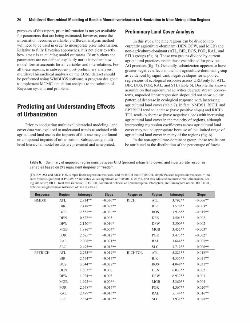
24 Multilevel Hierarchical Modeling of Benthic Macroinvertebrates to Urbanization in Nine Metropolitan Regions
purposes of this report, prior information is not yet available for parameters that are being estimated; however, once the information becomes available, a different analysis method will need to be used in order to incorporate prior information. Relative to fully Bayesian approaches, it is not clear exactly how lmer is calculating model estimates. Distributions and parameters are not defined explicitly nor is it evident how model format accounts for all variables and interrelations. For all these reasons, in subsequent post-preliminary analyses, multilevel hierarchical analysis on the EUSE dataset should be performed using WInBUGS software, a program designed to implement MCMC simulation analysis to the solution of Bayesian systems and problems.
Predicting and Understanding Effects of Urbanization
Prior to conducting multilevel hierarchal modeling, land cover data was explored to understand trends associated with agricultural land use as the impacts of this use may confound or compound impacts of urbanization. Subsequently, multi-level hierarchal model results are presented and interpreted.
Preliminary Land Cover Analysis
In this study, the nine regions can be divided into currently agriculture-dominant (DEN, DFW, and MGB) and non-agriculture-dominant (ATL, BIR, BOS, POR, RAL, and STL) groups (fig. 6). These two groups divided by current agricultural practices match those established for previous AG practices (fig. 7). Generally, urbanization appears to have greater negative effects in the non-agriculture-dominant group as evidenced by significant, negative slopes for unpooled regressions of ecological response across URB only for ATL, BIR, BOS, POR, RAL, and STL (table 6). Despite the known assumption that agricultural activities degrade stream ecosys-tems, unpooled linear regression slopes did not show a clear pattern of decrease in ecological response with increasing agricultural land cover (table 7). In fact, NMDS1, RICH, and EPTRICH tend to increase (have positive slope) and RICH-TOL tends to decrease (have negative slope) with increasing agricultural land cover in the majority of regions, although interpreting regression coefficients across agricultural land cover may not be appropriate because of the limited range of agricultural land cover in many of the regions (fig. 6).
In the non-agriculture-dominant group, these results can be attributed to the distribution of the percentage of forest
Table 6. Summary of unpooled regressions between URB (percent urban land cover) and invertebrate response variables based on 243 equivalent degrees of freedom.
[For NMDS1 and RICHTOL, simple linear regression was used, and for RICH and EPTRICH, simple Poisson regression was used; * indi-cates values significant at P<0.05; ** indicates values significant at P<0.001. NMDS1, first axis adjusted nonmetric multidimensional scal-ing site score; RICH, total taxa richness; EPTRICH, combined richness of Ephemeroptera, Plecoptera, and Trichoptera orders; RICHTOL, richness-weighted mean tolerance of taxa at a basin]
Response Region Intercept Slope Response Region Intercept Slope
NMDS1 ATL 2.814** –0.030** RICH ATL 3.792** –0.006**BIR 2.418** –0.023** BIR 3.578** –0.003*BOS 2.557** –0.036** BOS 3.938** –0.015**DEN 0.822** 0.005 DEN 3.504** –0.002DFW 2.120** –0.010* DFW 3.500** –0.002MGB 1.886** –0.007* MGB 3.452** –0.003*POR 2.685** –0.018** POR 3.473** –0.002*RAL 2.908** –0.021** RAL 3.644** –0.005**SLC 2.495** –0.018** SLC 3.712** –0.006**
EPTRICH ATL 2.753** –0.019** RICHTOL ATL 5.221** 0.018**BIR 2.654** –0.015** BIR 4.555** 0.021**BOS 3.044** –0.028** BOS 4.048** 0.031**DEN 1.803** 0.000 DEN 6.033** 0.002DFW 1.924** –0.003 DFW 6.937** –0.001MGB 1.992** –0.006* MGB 5.360** 0.004POR 2.548** –0.017** POR 4.367** 0.020**RAL 2.489** –0.016** RAL 5.144** 0.016**SLC 2.834** –0.018** SLC 3.931** 0.028**

Predicting and Understanding Effects of Urbanization 25
associated with the corresponding percentage of agriculture (fig. 12); that is, in ATL, BIR, BOS, and RAL, responses are likely to increase with increasing percentage of agriculture (table 7), not because agricultural practices yield positive effects on invertebrate communities, but more convincingly because percentage of agriculture is positively related to percentage of forest (fig. 12, ATL, BIR, BOS, and RAL graphs), whereas it is negatively associated with urbanization (fig. 13, ATL, BIR, BOS, and RAL graphs). Conversely, in POR and SLC, invertebrate communities show mostly insignificant responses to increasing percentage of agriculture (table 7), because there is more variation in the relations between percentage of agriculture and forest and urban land cover (figs. 12 and 13, POR and SLC graphs).
In contrast to the non-agriculture-dominant group, the agriculture-dominant group generally involves small percentages of forest (fig. 12); thus, agricultural land cover is nearly the inverse of urban land cover (fig. 13). The noticeable common feature in this agriculture-dominant group is that the assemblage metrics already reach low levels (or high levels in the case of RICHTOL) at the low range of both the urban and agricultural gradients (see intercepts in tables 6 and 7); accordingly, the rate of change in the responses along the gradients are relatively small or not detectable (see slopes in tables 6 and 7). However, in this group, low percentages of agriculture (or high urbanization) correspond consistently to the low levels of response, while high percentages of agricul-ture (or low urbanization) correspond to more variability in the responses (fig. 14), agreeing with results of previous studies (Wang and others, 2000).
Table 7. Summary of regressions between percentage of agriculture land-cover (NLDC7 and NLDC8) and invertebrate response variables based on 243 equivalent degrees of freedom.
[For NMDS1 and RICHTOL, simple linear regression was used, and for RICH and EPTRICH, simple Poisson regression was used; * indicates values significant at P<0.05; ** indicates values significant at P<0.001. NMDS1, first axis adjusted nonmetric multidimensional scaling site score; RICH, total taxa richness; EPTRICH, combined richness of Ephemeroptera, Plecoptera, and Trichoptera orders; RICH-TOL, richness-weighted mean tolerance of taxa at a basin]
Response Region Intercept Slope Response Region Intercept Slope
NMDS1 ATL 1.020** 0.049** RICH ATL 3.352** 0.014**BIR 0.850** 0.054** BIR 3.391** 0.006BOS 0.444 0.185** BOS 3.200** 0.060**DEN 1.340** –0.006 DEN 3.354** 0.001DFW 1.240** 0.011* DFW 3.383** 0.001MGB 1.402** 0.005 MGB 3.198** 0.002*POR 2.309** –0.010 POR 3.461** –0.002RAL 1.113** 0.056** RAL 3.205** 0.014**SLC 1.359** 0.012 SLC 3.345** 0.004
EPTRICH ATL 1.672** 0.031** RICHTOL ATL 6.334** –0.033*BIR 1.708** 0.031** BIR 5.988** –0.049**BOS 1.759** 0.106** BOS 5.852** –0.158**DEN 1.795** 0.000 DEN 6.142** –0.001DFW 1.705** 0.002 DFW 6.785** 0.002MGB 1.539** 0.004 MGB 5.512** –0.001POR 2.434** –0.015** POR 4.715** 0.013RAL 1.230** 0.039** RAL 6.472** –0.041**SLC 1.908** –0.004 SLC 5.713** –0.013

26 Multilevel Hierarchical Modeling of Benthic Macroinvertebrates to Urbanization in Nine Metropolitan Regions
Figure 12. Scatterplots of the percentage of agriculture (NLCD7 and NLCD8) compared to the percentage of forest (NLCD4 and NLCD5) for each region.
100
80
60
40
20
0
FOR
ES
T
100
80
60
40
20
0
FOR
ES
T
100
80
60
40
20
0
FOR
ES
T
0 20 40
AGRICULTURE
60 80 100 0 20 40
AGRICULTURE
60 80 100 0 20 40
AGRICULTURE
60 80 100
ATL BIR BOS
DEN DFW MGB
POR RAL SLC

Predicting and Understanding Effects of Urbanization 27
Figure 13. Scatterplots of the percentage of urban (NLCD2) compared to the percentage of agriculture (NLCD7 and NLCD8) for each region. [The filled squares represent the basins where percent forest (NLCD4 and NLCD5) is less than or equal to 33, the triangles represent the basins where percent forest (NLCD4 and NLCD5) is between 33 and 67, and the crosses represent the basins where percent forest (NLCD4 and NLCD5) is greater than or equal to 67]
ATL BIR BOS
DEN DFW MGB
POR RAL SLC
100
80
60
40
20
0
AG
RIC
ULT
UR
EA
GR
ICU
LTU
RE
AG
RIC
ULT
UR
E
100
80
60
40
20
0
100
80
60
40
20
00 20 40
URBAN
60 80 100 0 20 40
URBAN
60 80 100 0 20 40
URBAN
60 80 100

28 Multilevel Hierarchical Modeling of Benthic Macroinvertebrates to Urbanization in Nine Metropolitan Regions
Figure 14. Scatterplots of the percentage of agriculture (NLCD7 and NLCD8) compared to macroinvertebrate response variables (NMDS1, RICH, EPTRICH, and RICHTOL) for agriculture-dominant regions.
DEN DFW MGB
3.0
2.5
2.0
1.5
1.0
0.5
0
NM
DS
1R
ICH
EP
TRIC
H
50
45
40
35
30
25
20
15
10
5
0
RIC
HTO
L
8
7
6
5
40 20 40
AGRICULTURE
60 80 100 0 20 40
AGRICULTURE
60 80 100 0 20 40
AGRICULTURE
60 80 100

Predicting and Understanding Effects of Urbanization 29
Model Summary (Model Results)
Eight different multilevel hierarchical models of the form described in the Methods section, with varying region-level intercept and slope predictors, are fit to NMDS1, RICH, EPTRICH, and RICHTOL data from nine different regions. Deviance information criteria (DIC) are calculated (table 8) as a measure of goodness of fit across the eight models for each response variable. At the basin level, NMDS1 and RICHTOL models predict a continuous response from a continuous URB predictor using a linear regression, and RICH and EPTRICH models predict a discrete response from a continuous URB predictor using a generalized linear regression (Poisson data distribution with log link function). These regressions are defined by a set of nine region-level intercepts (αj) and nine slopes (βj), as well as a measure of average within-region variance ( )2
y for the linear regressions. The region-level slopes and intercepts themselves belong
to a higher tier distribution either centered on a constant pair of means (µ µα β and , Model 1), predicted from a linear regression with a region-level variable (Models 2–5),
or predicted from linear regressions with two region-level variables (Models 6–8). Each higher tier regression is defined by a hyperparameter intercept predicting region-level inter-cepts ( )0 , a hyperparameter slope predicting region-level intercepts ( )1 , between-region variance in intercept ( )2
, a hyperparameter intercept predicting region-level slopes ( )0 , a hyperparameter slope predicting region-level slopes ( )1 , and between-region variance in slope ( )2
. For the two region-level variable models, an additional term (δ) is added to hyperparameter intercept estimates to account for high (k=1) or low (k=0) antecedent agriculture. (See Model Structure section for model templates with coefficients.) Region-level annual precipitation and temperature are used as continuous variables (Models 2–4 and 6–8) , and region-level antecedent agricultural percentage is used as both a continuous (Model 5) and categorical variable (Models 6–8). When fit in R using the lmer or glmer commands, all models converge on peak values of posterior distributions of coefficients, calculated numerically using maximum likelihood estimation. Model coefficients are presented in tables 9–20. Model graphs are presented in figures 15–46.
Table 8. Deviance information criteria (DIC) for the eight different multilevel hierarchical models per response variable.
[NMDS1, first axis adjusted nonmetric multidimensional scaling site score; RICH, total taxa richness; EPTRICH, combined richness of Ephemeroptera, Plecoptera, and Trichoptera orders; RICHTOL, richness-weighted mean tolerance of taxa at a basin. See table 5 (p. 18) for model definitions]
Model 1 Model 2 Model 3 Model 4 Model 5 Model 6 Model 7 Model 8
NMDS1 499.5 472.8 489.9 484.0 462.2 471.4 479.5 474.4RICH 344.8 344.3 339.9 337.7 339.9 344.3 339.9 336.5EPTRICH 356.9 351.8 356.8 353.7 334.9 345.7 347.1 345.6RICHTOL 443.4 425.1 425.3 412.7 402.1 417.8 410.4 404.1

30 Multilevel Hierarchical Modeling of Benthic Macroinvertebrates to Urbanization in Nine Metropolitan Regions
Table 9. Intercept (α) and slope (β) coefficient estimates, representing background condition prior to urbanization and rate of change with urbanization, respectively, and variance coefficient estimates ( )2 2 2, , y for invertebrate response NMDS1 Model 1, unpooled model, and completely pooled model.
[N/A, not applicable because there are no α or β distributions for the unpooled and completely pooled models. Model 1 has only higher tier constant mean predictors ( µ µα β and ) and no group-level predictors, unpooled model addresses each region separately, and completely pooled model combines all regions]
Model 1 (Partially pooled) Unpooled Completely pooled
αj βj αunpooled βunpooled2ys α β
ATL 2.73 –2.80 2.81 –3.07 0.159 2.32 –1.60BIR 2.42 –2.24 2.42 –2.31 0.238BOS 2.50 –3.03 2.56 –3.57 0.144DEN 1.83 –0.74 1.67 –0.49 0.590DFW 2.15 –1.09 2.12 –0.97 0.575MGB 1.95 –0.84 1.89 –0.71 0.539POR 2.63 –1.84 2.69 –1.84 0.442RAL 2.76 –1.97 2.91 –2.10 0.193SLC 2.44 –1.69 2.50 –1.76 0.384
2y 0.360 Separate values for each j; see above 0.445
µα 2.378 N/A N/A
µβ –1.805 N/A N/A
2 0.139 N/A N/A
2 0.794 N/A N/A
Model 1: No Region-Level PredictorIn Model 1, each response variable is modeled hier-
archically from basin-level URB without any region-level predictors, allowing the intercept and slope to vary by region around constant means. In order to provide a benchmark for comparison, non-multilevel hierarchical linear regression models are also calculated. Completely pooled models are constructed by fitting a linear regression or generalized linear regression to data from all nine regions simultaneously while unpooled models are constructed by fitting a linear regression or generalized linear regression to each region independently. The results from these simple completely pooled and separate unpooled models are compared with Model l to understand how a hierarchical multilevel model bridges the gap between information obtained from these two modeling extremes.
NMDS1, RICH, and EPTRICH generally decrease with increasing urbanization while RICHTOL increases with increasing urbanization. These trends support the notion that the expansion of urban developed area co-occurred with detrimental effects on macroinvertebrate assemblages. While complete pooling of all nine regions summarize the aggregate pattern of decline with urbanization for each response,
unpooled models show that original conditions and response rates differ between regions.
For NMDS1, the negative trend of decreasing NMDS1 values with increasing urban land cover in complete pooling of all nine regions (fig. 15, dashed line) shows substantial scatter (table 9, 2
y = 0.445). When each region is modeled separately (fig. 15, black line), the unpooled regression models for POR, RAL, and SLC are similar to the completely pooled model. The unpooled models for ATL, BIR, and BOS have steeper slopes than the completely pooled, and the unpooled slopes of DFW, MGB, and DEN are statistically not different from zero. That is, the urbanization effects in POR, RAL, and SLC are close to the nine-region average, the effects in ATL, BIR, and BOS are above average (NMDS1 responds more to increasing urbanization than average), and the effects in DFW, MGB, and DEN are below average (NMDS1 responds less to increasing urbanization than average). Additionally, baseline NMDS1 values at no urbanization (intercepts) for unpooled models in BIR, BOS, DFW, and SLC are similar to completely pooled un-urbanized baseline. However, ATL, POR, and RAL appear to have higher NMDS1 values at no urbanization than overall average, while DEN and MGB have lower values at no urbanization than average.

Predicting and Understanding Effects of Urbanization 31
Figure 15. Scatterplots of NMDS1 compared to URB for each region with complete pooling, no pooling, and Model 1: No region-level predictors (eqs. 8 and 9, Template 1). [Dashed line, complete pooling; black line, no pooling; green line, Model 1 multilevel hierarchical partial pooling. NMDS1, nonmetric multidimensional scaling first axis ordination basin scores; URB, percentage of basin area in developed land]
ATL BIR BOS
DEN DFW MGB
POR RAL SLC
3.0
2.0
1.0
0
3.0
2.0
1.0
0
3.0
2.0
1.0
0
NM
DS
1N
MD
S1
NM
DS
1
0 20 40
URB
60 80 100 0 20 40
URB
60 80 100 0 20 40
URB
60 80 100

32 Multilevel Hierarchical Modeling of Benthic Macroinvertebrates to Urbanization in Nine Metropolitan Regions
Negative relations between RICH and percentage of urban land area in all nine regions (fig. 16; table 10) show between and within region variability, as well. Urbanization effects also vary among the nine regions with different intercepts and slope rates. The unpooled rate of change in total
richness with urbanization appears near average (completely pooled) for BIR, RAL, and SLC; below average in DEN, DFW, MGB, and POR; and above average in ATL. BOS, however, stands out as showing a substantially faster degrad-ing of RICH compared to other regions.
Table 10. Intercept (α) and slope (β) coefficient estimates, representing background condition prior to urbanization and rate of change with urbanization, respectively, and variance coefficient estimates ( )2 2 2, , y for invertebrate response RICH Model 1, unpooled model, and completely pooled model.
[N/A, not applicable because data variance is equal to the mean parameter (λ) in Poisson models and, therefore, changes with changing λj, and there are no α or β distributions for the unpooled and completely pooled models. Model 1 has only higher tier constant mean predictors ( µ µα β and ) and no group-level predictors, unpooled model addresses each region separately, and completely pooled model combines all regions]
Model 1 (Partially pooled) Unpooled Completely pooled
αj βj αunpooled βunpooledα β
ATL 3.78 –0.68 3.79 –0.62 3.62 –0.44BIR 3.58 –0.31 3.58 –0.28BOS 3.91 –1.26 3.94 –1.51DEN 3.51 –0.19 3.50 –0.16DFW 3.51 –0.19 3.50 –0.17MGB 3.48 –0.27 3.45 –0.29POR 3.49 –0.24 3.47 –0.24RAL 3.64 –0.50 3.64 –0.50SLC 3.68 –0.55 3.71 –0.59
2y N/A N/A N/A
µα 3.618 N/A N/A
µβ –0.467 N/A N/A
2 0.022 N/A N/A
2 0.116 N/A N/A

Predicting and Understanding Effects of Urbanization 33
Figure 16. Scatterplots of RICH compared to URB for each region with complete pooling, no pooling, and Model 1: No region-level predictors (eqs. 8 and 9, Template 1). [Dashed line, complete pooling; black line, no pooling; green line, Model 1 multilevel hierarchical partial pooling. RICH, total taxa richness; URB, percentage of basin area in developed land]
ATL BIR BOS
DEN DFW MGB
POR RAL SLC
60
50
40
30
20
60
50
40
30
20
60
50
40
30
20
RIC
HR
ICH
RIC
H
0 20 40
URB
60 80 100 0 20 40
URB
60 80 100 0 20 40
URB
60 80 100
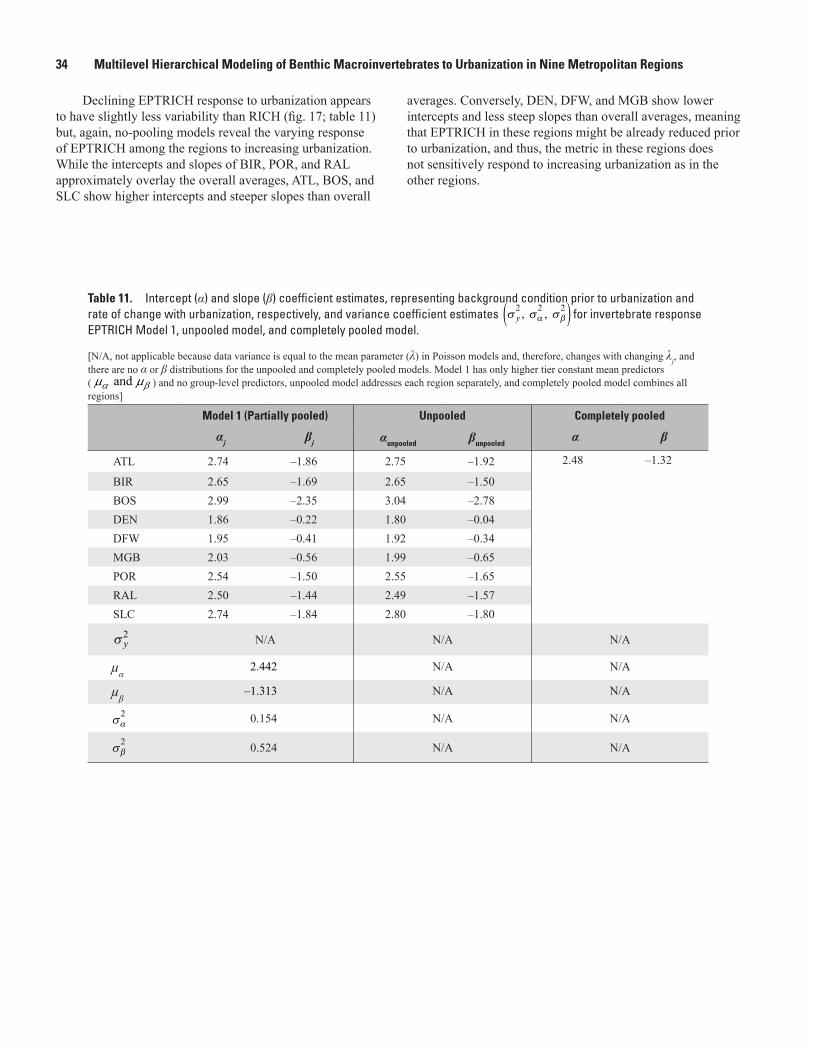
34 Multilevel Hierarchical Modeling of Benthic Macroinvertebrates to Urbanization in Nine Metropolitan Regions
Declining EPTRICH response to urbanization appears to have slightly less variability than RICH (fig. 17; table 11) but, again, no-pooling models reveal the varying response of EPTRICH among the regions to increasing urbanization. While the intercepts and slopes of BIR, POR, and RAL approximately overlay the overall averages, ATL, BOS, and SLC show higher intercepts and steeper slopes than overall
averages. Conversely, DEN, DFW, and MGB show lower intercepts and less steep slopes than overall averages, meaning that EPTRICH in these regions might be already reduced prior to urbanization, and thus, the metric in these regions does not sensitively respond to increasing urbanization as in the other regions.
Table 11. Intercept (α) and slope (β) coefficient estimates, representing background condition prior to urbanization and rate of change with urbanization, respectively, and variance coefficient estimates ( )2 2 2, , y for invertebrate response EPTRICH Model 1, unpooled model, and completely pooled model.
[N/A, not applicable because data variance is equal to the mean parameter (λ) in Poisson models and, therefore, changes with changing λj, and there are no α or β distributions for the unpooled and completely pooled models. Model 1 has only higher tier constant mean predictors ( µ µα β and ) and no group-level predictors, unpooled model addresses each region separately, and completely pooled model combines all regions]
Model 1 (Partially pooled) Unpooled Completely pooled
αj βj αunpooled βunpooledα β
ATL 2.74 –1.86 2.75 –1.92 2.48 –1.32
BIR 2.65 –1.69 2.65 –1.50BOS 2.99 –2.35 3.04 –2.78DEN 1.86 –0.22 1.80 –0.04DFW 1.95 –0.41 1.92 –0.34MGB 2.03 –0.56 1.99 –0.65POR 2.54 –1.50 2.55 –1.65RAL 2.50 –1.44 2.49 –1.57SLC 2.74 –1.84 2.80 –1.80
2y N/A N/A N/A
µα 2.442 N/A N/A
µβ –1.313 N/A N/A
2 0.154 N/A N/A
2 0.524 N/A N/A

Predicting and Understanding Effects of Urbanization 35
Figure 17. Scatterplots of EPTRICH compared to URB for each region with complete pooling, no pooling, and Model 1: No region-level predictors (eqs. 8 and 9, Template 1). [Dashed line, complete pooling; black line, no pooling; green line, Model 1 multilevel hierarchical partial pooling. EPTRICH, combined richness of Ephemeroptera, Plecoptera, and Trichoptera orders; URB, percentage of basin area in developed land]
ATL BIR BOS
DEN DFW MGB
POR RAL SLC
25
20
15
10
5
0
25
20
15
10
5
0
25
20
15
10
5
0
EP
TRIC
HE
PTR
ICH
EP
TRIC
H
0 20 40
URB
60 80 100 0 20 40
URB
60 80 100 0 20 40
URB
60 80 100

36 Multilevel Hierarchical Modeling of Benthic Macroinvertebrates to Urbanization in Nine Metropolitan Regions
Finally, the complete pooling of RICHTOL across all nine regions (fig. 18, dashed line) shows a pattern opposite the other three metrics. While total richness, EPT richness, and ordination scores scaled to EPT richness decrease with urbanization, richness-weighted tolerance generally increases with increasing urban land cover. Overall, this pattern shows considerable scatter (table 12, 2
y = 0.704), greater than that for NMDS1. Modeled individually, POR, MGB, and SLC have the greatest within-region variability in RICHTOL response to urban land cover (table 12, 2
y = 0.555, 0.389, 0.354, respectively). The unpooled regressions (fig. 18, black line) match the slope of the completely pooled model fairly well in BIR, ATL, RAL, and POR but exhibit steeper slopes than the slope of the completely pooled model for BOS and SLC and flatter slopes than those calculated in the completely pooled model for MGB, DFW, and DEN. This means that the RICHTOL in BOS and SLC responds more drastically to increasing urbanization than the overall average, while in MGB, DFW, and DEN the rate at which RICHTOL increases is less affected by increases in urbanization as compared to the overall average.
Multilevel hierarchical Model 1 combines data from an individual region with the overall trend from the nine regions to calculate partially pooled estimates of intercept (αj) and slope (βj) for each region, as well as estimates of within-region variance in invertebrate response ( )2
y , between-region
variance in intercept ( )2 , and between-region variance in
slope ( )2 for each of the four ecological response models.
As in the simple linear regressions, the multilevel hierarchical model intercept represents the estimated value of the ecologi-cal metric at zero urbanization, and the slope represents the rate of change of the ecological metric with urbanization. However, the difference is that multilevel hierarchical model estimates are calculated taking into account both the regional data and the overall data across all regions. These partially pooled αj and βj values are, therefore, shrunk toward the overall mean. For example, the estimated Model 1 NMDS1 αj value for ATL (2.73, table 9) is a partial pooling of intercept information from the unpooled NMDS1 ATL model (2.81, table 9) and intercept information from the overall completely pooled NMDS1 model (2.32, table 9).
By assigning multilevel hierarchical structure to the data, individual region estimates borrow strength from the entire dataset and decrease the biasing influence of group sample size. In this analysis, all of the nine regions have approxi-mately equal sample sizes (28–30). Also, between-region variance is generally greater than within-region variance, meaning that the pattern of ecological response to urbanization varies substantially from region to region for each response variable. Therefore, unpooled regressions have greater weight than the completely pooled regression on partially pooled estimates. This is why, although the partially pooled multilevel
Table 12. Intercept (α) and slope (β) coefficient estimates, representing background condition prior to urbanization and rate of change with urbanization, respectively, and variance coefficient estimates ( )2 2 2, , y for invertebrate response RICHTOL Model 1, unpooled model, and completely pooled model.
[N/A, not applicable because there are no α or β distributions for the unpooled and completely pooled models. Model 1 has only higher tier con-stant mean predictors ( µ µα β and ) and no group-level predictors, unpooled model addresses each region separately, and completely pooled model combines all regions]
Model 1 (Partially pooled) Unpooled Completely pooled
αj βj αunpooled βunpooled2ys α β
ATL 5.26 1.60 5.22 1.75 0.122 5.20 1.22BIR 4.58 2.13 4.55 2.11 0.231BOS 4.12 2.75 4.05 3.05 0.187DEN 5.98 0.21 6.03 0.16 0.226DFW 6.92 –0.16 6.94 –0.06 0.282MGB 5.32 0.59 5.36 0.35 0.389POR 4.37 2.12 4.37 1.98 0.555RAL 5.15 1.55 5.14 1.57 0.131SLC 4.01 2.60 3.93 2.83 0.354
2y 0.275 Separate values for each j; see above 0.704
µα 5.079 N/A N/A
µβ 1.482 N/A N/A
2 0.916 N/A N/A
2 1.169 N/A N/A

Predicting and Understanding Effects of Urbanization 37
Figure 18. Scatterplots of RICHTOL compared to URB for each region with complete pooling, no pooling, and Model 1: No region-level predictors (eqs. 8 and 9, Template 1). [Dashed line, complete pooling; black line, no pooling; green line, Model 1 multilevel hierarchical partial pooling. RICHTOL, richness-weighted mean tolerance of taxa at a basin; URB, percentage of basin area in developed land]
ATL BIR BOS
DEN DFW MGB
POR RAL SLC
8
7
6
5
4
8
7
6
5
4
8
7
6
5
4
RIC
HTO
LR
ICH
TOL
RIC
HTO
L
0 20 40
URB
60 80 100 0 20 40
URB
60 80 100 0 20 40
URB
60 80 100

38 Multilevel Hierarchical Modeling of Benthic Macroinvertebrates to Urbanization in Nine Metropolitan Regions
hierarchical models (figs. 15–18, green lines, for NMDS1, RICH, EPTRICH, and RICHTOL, respectively) technically lie between their respective completely pooled and separate unpooled regressions for each region (figs. 15–18, dashed and black lines, for NMDS1, RICH, EPTRICH, and RICHTOL, respectively), they do not appear to differ significantly from results obtained by separate unpooled regressions. This trend holds for Models 2–8 and, therefore, the visual model results at the basin level are not depicted for the remaining models. Since Model 1 imposes a higher tier distribution structure on the data by assuming that slopes and intercepts for the nine regions are drawn from the same distribution, residual vari-ance decreases for the linear multilevel hierarchical models ( 2
y = 0.360 and 0.275, for NMDS1 and RICHTOL, table 9 and table 12, respectively) relative to the completely pooled models ( 2
y = 0.445 and 0.704, for NMDS1 and RICHTOL, table 9 and table 12, respectively) which has no higher tier structure requirement. Poisson model variance is not held constant by definition and, therefore, the same comparison cannot be made for RICH and EPTRICH.
Because it does not incorporate region-level data, Model 1 assumes that slopes and intercepts for regions are exchangeable and are drawn from the same distribution centered on a constant, µ. When region-level variables are available, however, differences in slope and intercept between regions are no longer random. These differences can now be explained by differences in region-level variable values, as shown below. In this way, multilevel hierarchical analysis incorporates data measured at different scales into the same model and enables multilevel hierarchical models to harness greater interpretive power than simple single-tier regression.
Model 2: PRECIP Region-Level Predictor
Unlike Model 1, Models 2–8 assume that differences between regions in response to urbanization are not random but mediated by physical environmental factors. Model 2 uses the differences in annual precipitation between the nine regions to account for differences in regional intercept and slope. Partially pooled estimates of intercept (αj) and slope (βj) for each region, within-region variance in invertebrate response ( )2
y , between-region variance in intercept ( )2
, and between-region variance in slope ( )2 are again
calculated for each of the four ecological response models. In addition, Model 2 estimates region-level intercepts and slopes ( )0 1 0 1, , , and which describe the relation between the regional precipitation predictor and αj and βj. This means that in Model 2, 2
and 2 now describe variation of
estimated intercepts and slopes around a higher tier regression line, instead of variation around a constant mean as in Model 1. Incorporating a regional, explanatory variable into intercept and slope estimation results in better model fit for all four response variables, as measured by lower DIC for Model 2 (and all subsequent Models) relative to Model 1 (table 8).
When precipitation is included as a region-level predic-tor, NMDS1 (fig. 19; table 13), RICH (fig. 20; table 14), and EPTRICH (fig. 21; table 15) intercepts increase with increas-ing precipitation and their slopes become more negative with increasing precipitation. Conversely, RICHTOL intercepts decrease with increasing precipitation and slopes become more steeply positive with increasing precipitation (fig. 22; table 16). This finding means that precipitation affects both baseline pre-urbanization conditions and rate of change in ecological condition with urbanization.
Because NMDS1 scores are scaled such that they decrease from a maximum value at minimum urban intensity to zero at maximum urban intensity, the intercept provides a measure of the approximate extent to which the assemblages at minimum and maximum urbanization (URB) differ. Regions with little precipitation have lower intercepts than do regions with higher precipitation (fig. 19A). Consequently, the amount of change that can occur over the urbanization gradient is lower in regions with lower precipitation. This finding is also reflected in the slopes (fig. 19B), which are higher in regions with higher precipitation and lower in regions with lower precipitation. That is, given a minimum possible low NMDS1 value of zero, higher NMDS1 starting values have more parameter space in which to fall. This correlation between intercept and slope is addressed with the ρ model coefficient term.
RICH and EPTRICH metrics are absolute, not scaled, measures of total and EPT taxa richness. Higher precipitation is also associated with greater total richness and greater EPT richness at zero urbanization, although both relations look considerably more scattered than NMDS1 Model 2. This greater initial richness results in more negative rates of change of richness with urbanization at high precipitation, and lower initial richness at low precipitation results in the opposite (less negative rates of change of richness with urbanization). RICHTOL metrics are richness weighted and defined on a scale of 0 to 10. However, RICHTOL values in the EUSE dataset range from only 4 to 7, showing that typical macroin-vertebrate communities were neither completely tolerant nor completely intolerant. Following expected response direction of the previous three variables, higher precipitation was associated with lower richness-weighted tolerance and steeper increase in tolerance with urbanization. Similar to NMDS1, RICHTOL intercepts and slopes also show inverse correlation, lending ecological credence to observed patterns.
Therefore, in addition to response shapes derived from statistical consequences, Model 2 is scientifically interpretable. In general, macroinvertebrate condition metrics appear to be worse in dry regions with little precipitation and better in wet regions with greater precipitation prior to urbanization. This can be interpreted to mean that wet regions are likely associ-ated with greater indicators of healthier stream macroinver-tebrate communities than dry regions in the absence of urban land cover. Precipitation also appears to speed up the decline of macroinvertebrate communities with urbanization.

Predicting and Understanding Effects of Urbanization 39
Table 13. Regional intercept (αj) and slope (β
j) coefficient estimates, representing regional background condition prior to
urbanization and regional rate of change with urbanization, respectively, hyperparameter intercept and slope coefficient estimates ( 0 1 0 1, , , and ), and variance coefficient estimates ( )2 2 2, , y for invertebrate response NMDS1 Models 2–5.
[See table 5 (p. 18) for model definitions]
Model 2 Model 3 Model 4 Model 5
αj βj αj βj αj βj αj βj
ATL 2.71 –2.77 2.76 –2.86 2.73 –2.77 2.60 –2.44BIR 2.55 –2.49 2.44 –2.30 2.43 –2.29 2.59 –2.60BOS 2.49 –3.06 2.49 –3.09 2.44 –3.02 2.50 –3.07DEN 1.72 –0.56 1.80 –0.70 1.80 –0.69 1.83 –0.75DFW 2.18 –1.16 2.18 –1.10 2.19 –1.11 1.98 –0.68MGB 1.98 –0.88 1.92 –0.80 1.94 –0.85 1.96 –0.85POR 2.71 –1.98 2.61 –1.81 2.64 –1.91 2.75 –2.08RAL 2.69 –1.86 2.78 –1.98 2.81 –2.01 2.69 –1.83SLC 2.19 –1.32 2.39 –1.632 2.42 –1.65 2.78 –2.24
2y 0.360 0.359 0.359 0.359
0 1.407 1.901 1.948 2.818
1 0.009 0.0383 0.035 –0.011
0 0.240 –1.199 –0.836 –2.784
1 –0.019 –0.049 –0.009 0.024
2 0.046 0.139 0.134 0.0162 0.436 0.922 0.551 0.108
Figure 19. NMDS1 multilevel hierarchical Model 2: Region-level precipitation predictor for (A) intercept and (B) slope. Within each region, NMDS1 (first axis adjusted nonmetric multidimensional scaling site score) is modeled as a linear function of URB (percent urban land cover) as shown in eq. 10 (Template 2, basin level). Across regions, intercepts (A) and slopes (B) are modeled as a function of regional precipitation as shown in eq. 11 (Template 2, region level).
BIR
BOS
DEN
DFW
MGB
PORRALATL
SLC
40 60 80 100 120 140 160REGION−LEVEL ANNUAL PRECIPITATION, IN CENTIMETERS
40 60 80 100 120 140 160REGION−LEVEL ANNUAL PRECIPITATION, IN CENTIMETERS
ES
TIM
ATE
D S
LOP
E, ß
j
BIR
BOS
DEN
DFW
MGB
PORRAL
SLC
A B
–0.5
–1.0
–1.5
–2.0
–2.5
–3.0
–3.5
ES
TIM
ATE
D IN
TER
CE
PT,
αj
3.0
2.8
2.6
2.4
2.2
2.0
1.8
1.6
ATL

40 Multilevel Hierarchical Modeling of Benthic Macroinvertebrates to Urbanization in Nine Metropolitan Regions
Figure 20. RICH multilevel hierarchical Model 2: Region-level precipitation predictor for (A) intercept and (B) slope. Within each region, RICH (total taxa richness) is modeled as a log-linear function of URB (percent urban land cover) as shown in eqs. 18 and 19 (Template 2, basin level). Across regions, intercepts (A) and slopes (B) are modeled as a function of regional precipitation as shown in eq. 11 (Template 2, region level).
Table 14. Regional intercept (αj) and slope (β
j) coefficient estimates, representing regional background condition prior to
urbanization and regional rate of change with urbanization, respectively, hyperparameter intercept and slope coefficient estimates ( 0 1 0 1, , , and ), and variance coefficient estimates ( )2 2 2, , y for invertebrate response RICH Models 2–5.
[N/A, not applicable because data variance is equal to the mean parameter (λ) in Poisson models and, therefore, changes with changing λj. See table 5 (p. 18) for model definitions]
Model 2 Model 3 Model 4 Model 5
αj βj αj βj αj βj αj βj
ATL 3.78 –0.69 3.78 –0.68 3.79 –0.75 3.78 –0.68BIR 3.58 –0.32 3.58 –0.29 3.58 –0.34 3.60 –0.34BOS 3.91 –1.26 3.90 –1.25 3.90 –1.19 3.90 –1.25DEN 3.50 –0.18 3.49 –0.21 3.50 –0.19 3.49 –0.15DFW 3.51 –0.19 3.52 –0.13 3.53 –0.09 3.49 –0.18MGB 3.48 –0.27 3.48 –0.29 3.47 –0.26 3.47 –0.26POR 3.50 –0.25 3.49 –0.24 3.48 –0.29 3.51 –0.27RAL 3.64 –0.50 3.65 –0.50 3.66 –0.50 3.65 –0.51SLC 3.67 –0.53 3.64 –0.52 3.64 –0.53 3.70 –0.58
2y N/A N/A N/A N/A
0 3.510 3.602 3.442 3.742
1 0.001 0.001 0.014 –0.003
0 –0.226 –0.723 –0.273 –0.718
1 –0.002 0.021 –0.002 0.0062 0.020 0.021 0.023 0.0122 0.111 0.111 0.104 0.075
40 60 80 100 120 140 160REGION−LEVEL ANNUAL PRECIPITATION, IN CENTIMETERS
40 60 80 100 120 140 160REGION−LEVEL ANNUAL PRECIPITATION, IN CENTIMETERS
ES
TIM
ATE
D S
LOP
E, ß
j
A B
–0.2
–0.4
–0.6
–0.8
–1.0
–1.2
–1.4
ES
TIM
ATE
D IN
TER
CE
PT,
αj
4.0
3.9
3.8
3.7
3.6
3.5
ATL
BIR
BOS
DEN DFWMGB
POR
RALSLC
ATL
BIR
BOS
DEN DFWMGB POR
RALSLC
FIG 20

Predicting and Understanding Effects of Urbanization 41
Figure 21. EPTRICH multilevel hierarchical Model 2: Region-level precipitation predictor for (A) intercept and (B) slope. Within each region, EPTRICH (combined richness of Ephemeroptera, Plecoptera, and Trichoptera orders) is modeled as a log-linear function of URB (percent urban land cover) as shown in eqs. 18 and 19 (Template 2, basin level). Across regions, intercepts (A) and slopes (B) are modeled as a function of regional precipitation as shown in eq. 11 (Template 2, region level).
Table 15. Regional intercept (αj) and slope (β
j) coefficient estimates, representing regional background condition prior to
urbanization and regional rate of change with urbanization, respectively, hyperparameter intercept and slope coefficient estimates ( 0 1 0 1, , , and ), and variance coefficient estimates ( )2 2 2, , y for invertebrate response EPTRICH Models 2–5.
[N/A, not applicable because data variance is equal to the mean parameter (λ) in Poisson models and, therefore, changes with changing λj. See table 5 (p. 18) for model definitions]
Model 2 Model 3 Model 4 Model 5
αj βj αj βj αj βj αj βj
ATL 2.75 –1.91 2.74 –1.84 2.74 –1.83 2.73 –1.84BIR 2.69 –1.85 2.65 –1.67 2.68 –1.80 2.70 –1.75BOS 2.99 –2.30 3.00 –2.37 3.00 –2.40 2.94 –2.28DEN 1.83 –0.12 1.85 –0.23 1.86 –0.17 1.80 –0.15DFW 1.96 –0.50 1.95 –0.38 1.95 –0.37 1.91 –0.36MGB 2.02 –0.55 2.03 –0.58 2.01 –0.64 1.97 –0.48POR 2.56 –1.64 2.54 –1.51 2.55 –1.73 2.63 –1.60RAL 2.50 –1.45 2.50 –1.43 2.49 –1.40 2.59 –1.55SLC 2.72 –1.70 2.74 –1.84 2.78 –1.79 2.75 –1.86
2y N/A N/A N/A N/A
0 1.729 2.444 2.269 2.926
1 0.007 0.000 0.014 –0.012
0 0.165 –1.373 –0.886 –2.183
1 –0.014 0.005 –0.004 0.0232 0.105 0.154 0.162 0.0082 0.307 0.530 0.442 0.041
40 60 80 100 120 140 160REGION−LEVEL ANNUAL PRECIPITATION, IN CENTIMETERS
40 60 80 100 120 140 160REGION−LEVEL ANNUAL PRECIPITATION, IN CENTIMETERS
ßjE
STI
MA
TED
SLO
PE
, ßj
A B
0
–0.5
–1.0
–1.5
–2.0
–2.5
ES
TIM
ATE
D IN
TER
CE
PT,
αj
3.0
2.8
2.6
2.4
2.2
2.0
1.8
ATLBIR
BOS
DEN
DFWMGB
POR
SLC
RAL
ATLBIR
BOS
DEN
DFWMGB
PORSLC
RAL
FIG 21

42 Multilevel Hierarchical Modeling of Benthic Macroinvertebrates to Urbanization in Nine Metropolitan Regions
Figure 22. RICHTOL multilevel hierarchical Model 2: Region-level precipitation predictor for (A) intercept and (B) slope. Within each region, RICHTOL (richness-weighted mean tolerance of taxa at a basin) is modeled as a linear function of URB (percent urban land cover) as shown in eq. 10 (Template 2, basin level). Across regions, intercepts (A) and slopes (B) are modeled as a function of regional precipitation as shown in eq. 11 (Template 2, region level).
Table 16. Regional intercept (αj) and slope (β
j) coefficient estimates, representing regional background condition prior to
urbanization and regional rate of change with urbanization, respectively, hyperparameter intercept and slope coefficient estimates ( 0 1 0 1, , , and ), and variance coefficient estimates ( )2 2 2, , y for invertebrate response RICHTOL Models 2–5.
[See table 5 (p. 18) for model definitions]
Model 2 Model 3 Model 4 Model 5
αj βj αj βj αj βj αj βj
ATL 5.25 1.60 5.25 1.63 5.26 1.55 5.17 1.87BIR 4.55 2.13 4.53 2.32 4.52 2.41 4.53 2.19BOS 4.11 2.75 4.16 2.41 4.21 2.05 4.19 2.43DEN 6.01 0.21 6.01 0.14 5.99 0.21 6.10 0.00DFW 6.92 –0.16 6.93 –0.19 6.92 –0.22 6.94 –0.22MGB 5.32 0.59 5.32 0.62 5.32 0.67 5.35 0.50POR 4.35 2.12 4.36 2.12 4.38 1.93 4.31 2.25RAL 5.15 1.55 5.15 1.58 5.15 1.60 5.04 1.78SLC 4.06 2.60 4.03 2.62 4.00 2.71 4.19 2.39
2y 0.274 0.275 0.278 0.272
0 6.032 3.786 3.937 4.171
1 –0.009 0.104 0.092 0.024
0 0.078 1.989 1.962 2.656
1 0.013 –0.042 –0.005 –0.0312 0.924 0.850 0.745 0.2752 1.088 1.263 1.245 0.049
40 60 80 100 120 140 160REGION−LEVEL ANNUAL PRECIPITATION, IN CENTIMETERS
40 60 80 100 120 140 160REGION−LEVEL ANNUAL PRECIPITATION, IN CENTIMETERS
ES
TIM
ATE
D S
LOP
E, ß
j
A B
ES
TIM
ATE
D IN
TER
CE
PT,
αj
7.0
6.5
6.0
5.5
5.0
4.5
4.0
3.0
2.5
2.0
1.5
1.0
0.5
0
–0.5
ATL
BIR
BOS
DEN
DFW
MGB
RAL
POR
SLC
ATL
BIR
BOS
DEN
DFW
MGB
POR
SLC
RAL
FIG 22

Predicting and Understanding Effects of Urbanization 43
Model 3: TEMP Region-Level Predictor
Model 3 replaces annual precipitation with annual temperature as a region-level intercept and slope predictor. Model format and coefficient interpretations are identical to Model 2, exchanging TEMP for PRECIP. In contrast to models including precipitation, only NMDS1 and RICHTOL appear to respond to temperature, while RICH and EPTRICH, for the most part, do not.
For NMDS1, Model 3 goodness of model fit evaluated visually and quantitatively (DIC = 489.9, table 8) is less than the fit of Model 2 (DIC = 472.8, table 8). Nonetheless, there is still a fairly strong increase in intercept with increasing temperature (fig. 23A; table 13) and increase in negative slope steepness with increasing temperature (fig. 23B; table 13). Decline in NMDS1 with urbanization (in all regions except DEN) appears to happen faster in regions with warmer temperatures. The negative relation of slope with temperature is not very strong, and regions such as BOS, DEN, and DFW do not follow this pattern closely.
Temperature does not appear to have any effect on RICH prior to urbanization (fig. 24A; table 14). Total richness prior to urbanization appears to vary randomly across both colder regions (such as SLC and MGB) and warmer regions (such as ATL and DFW). Somewhat of a pattern with temperature is observed under urbanization conditions. There appears to be less decline in total richness per unit change of urbanization
with warmer temperature (fig. 24B), which implies that warmer climate is more optimal for high total macroinver-tebrate richness. However, this response to temperature is driven largely by a BOS outlier, which has an estimated slope substantially more negative than the remaining regions and also the second coldest annual temperature. Without the BOS point, it appears that slope estimates vary randomly with temperature, as well. Therefore, it is surprising that DIC assigns better model fit to Model 3 (DIC = 339.9, table 8) than to Model 2 (DIC = 344.3, table 8) for RICH data. It is not clear why this occurs.
For EPTRICH, adding a region-level predictor did not significantly reduce the DIC (356.8, table 8), nor significantly improve the accuracy in estimating coefficients at region level ( 2
= 0.154 and 2 = 0.524 for Model 1 [table 11]
relative to 2 = 0.105 and 2
= 0.307 for Model 2 and 2 = 0.154 and 2
= 0.530 for Model 3 [table 15]). In fact, adding a region-level predictor actually slightly increased the unexplained region-level variance for Model 3 slope. One potential reason of this result could be the similar sample sizes (27 to 30) among regions, which minimizes the level of pooling effect toward the overall mean, thus also minimizing the degree of modifying 2
and 2 , which is usually done
through partial pooling. Another possibility could be that 2 and 2
increase because adding a region-level predictor actually unveils the hidden variation among regions by explaining correlation between the basin-level variable (URB)
Figure 23. NMDS1 multilevel hierarchical Model 3: Region-level temperature predictor for (A) intercept and (B) slope. Within each region, NMDS1 (first axis adjusted nonmetric multidimensional scaling site score) is modeled as a linear function of URB (percent urban land cover) as shown in eq. 10 (Template 2, basin level). Across regions, intercepts (A) and slopes (B) are modeled as a function of regional temperature as shown in eq. 11 (Template 2, region level).
8 10 12 14 16 18 20REGION−LEVEL ANNUAL TEMPERATURE, IN DEGREES CELSIUS
8 10 12 14 16 18 20REGION−LEVEL ANNUAL TEMPERATURE, IN DEGREES CELSIUS
ES
TIM
ATE
D S
LOP
E, ß
j
A B
ES
TIM
ATE
D IN
TER
CE
PT,
αj
3.0
2.8
2.6
2.4
2.2
2.0
1.8
1.6
–0.5
–1.0
–1.5
–2.0
–2.5
–3.0
–3.5
ATL
BIRBOS
SLC
DEN
DFW
MGB
POR
RAL
ATL
BIR
BOS
DEN
DFW
MGB
PORRAL
SLC
FIG 23

44 Multilevel Hierarchical Modeling of Benthic Macroinvertebrates to Urbanization in Nine Metropolitan Regions
and region-level errors ( )2 2 and (Gelman and Hill 2006). Nonetheless, a region-level predictor still improves the model with regard to interpretability of region-level variations. Estimated intercepts and slopes do not show any significant tendency (of increasing or decreasing) along with changes in annual mean temperature (fig. 25). This result indicates that influential factors other than temperature likely determine the response of EPTRICH at the region-level. One of the potential factors might be the level of agricultural activities at each region because the regions that deviated from the others, by having lower intercepts and higher slopes, are the agriculture-dominant group (DEN, MGB, DFW; see Preliminary Land Cover Analysis section).
For RICHTOL, Model 3 seems to fit (DIC = 425.3, table 8) the data as well as Model 2 (DIC = 425.1, table 8). Nonetheless, in Model 3 the intercept increases with
increasing temperature (fig. 26A; table 16), while the positive slope on urban development tends to decrease with increasing temperatures (fig. 26B; table 16). Prior to urbanization, it appears that there are more tolerant species in warmer regions. And the positive relation between RICHTOL and urban development dampens slightly as regional mean annual ambient temperature increases. This could mean that warmer regions initially start with more hardy species and as such they have less opportunity to gain even more hardy species with increasing urbanization. This dampening of the slope with increased temperature does not seem to be strong for regions such as MGB and DEN, which have flat slopes despite low mean temperatures. Again, it appears that high-agriculture regions (DEN, DFW, MGB) form a response group pattern visually separate from the remaining regions.
Figure 24. RICH multilevel hierarchical Model 3: Region-level temperature predictor for (A) intercept and (B) slope. Within each region, RICH (total taxa richness) is modeled as a log-linear function of URB (percent urban land cover) as shown in eqs. 18 and 19 (Template 2, basin level). Across regions, intercepts (A) and slopes (B) are modeled as a function of regional temperature as shown in eq. 11 (Template 2, region level).
8 10 12 14 16 18 20
REGION−LEVEL ANNUAL TEMPERATURE, IN DEGREES CELSIUS
8 10 12 14 16 18 20
REGION−LEVEL ANNUAL TEMPERATURE, IN DEGREES CELSIUSE
STI
MA
TED
SLO
PE
, ßj
A B
ES
TIM
ATE
D IN
TER
CE
PT,
αj
3.9
3.8
3.7
3.6
3.5
0
–0.2
–0.4
–0.6
–0.8
–1.0
–1.2
–1.4
ATL
BIR
BOS
DENDFW
MGBPOR
RALSLC
ATL
BIR
DENDFW
MGBPOR
RALSLC
FIG 24

Predicting and Understanding Effects of Urbanization 45
Figure 25. EPTRICH multilevel hierarchical Model 3: Region-level temperature predictor for (A) intercept and (B) slope. Within each region, EPTRICH (combined richness of Ephemeroptera, Plecoptera, and Trichoptera orders) is modeled as a log-linear function of URB (percent urban land cover) as shown in eqs. 18 and 19 (Template 2, basin level). Across regions, intercepts (A) and slopes (B) are modeled as a function of regional temperature as shown in eq. 11 (Template 2, region level).
Figure 26. RICHTOL multilevel hierarchical Model 3: Region-level temperature predictor for (A) intercept and (B) slope. Within each region, RICHTOL (richness-weighted mean tolerance of taxa at a basin) is modeled as a linear function of URB (percent urban land cover) as shown in eq. 10 (Template 2, basin level). Across regions, intercepts (A) and slopes (B) are modeled as a function of regional temperature as shown in eq. 11 (Template 2, region level).
8 10 12 14 16 18 20REGION−LEVEL ANNUAL TEMPERATURE, IN DEGREES CELSIUS
8 10 12 14 16 18 20REGION−LEVEL ANNUAL TEMPERATURE, IN DEGREES CELSIUS
ES
TIM
ATE
D S
LOP
E, ß
j
A B
ES
TIM
ATE
D IN
TER
CE
PT,
αj
3.0
2.8
2.6
2.4
2.2
2.0
1.8
0
–0.5
–1.0
–1.5
–2.0
–2.5
ATL
BIR
BOS
SLC
DEN
DFWMGB
PORRAL
ATL
BIR
BOS
DEN
DFW
MGB
PORRAL
SLC
8 10 12 14 16 18 20REGION−LEVEL ANNUAL TEMPERATURE, IN DEGREES CELSIUS
8 10 12 14 16 18 20REGION−LEVEL ANNUAL TEMPERATURE, IN DEGREES CELSIUS
ES
TIM
ATE
D S
LOP
E, ß
j
A B
ES
TIM
ATE
D IN
TER
CE
PT,
αj
7.0
6.5
6.0
5.5
5.0
4.5
4.0
3.0
2.5
2.0
1.5
1.0
0.5
0
–0.5
BIR
BOS
DEN
DFW
MGB
POR
RALATL
SLC
ATL
BIRBOS
DEN
DFW
MGB
POR
RAL
SLC

46 Multilevel Hierarchical Modeling of Benthic Macroinvertebrates to Urbanization in Nine Metropolitan Regions
Model 4: PRECIP and TEMP Region-Level Predictors
Model 4 combines the most scientifically plausible climate region-level predictors into one model where intercept varies with temperature, and slope varies with precipitation. The intent is to account for the possibility that temperature governs the baseline ecological response at pre-urbanization, while precipitation governs the rate of change in ecological response with urban development. In this model, partially pooled estimates of basin-level intercept (αj) are modeled at the region level as a linear function of TEMP using region-level intercept, 0 , and region-level slope, 1 . Meanwhile, partially pooled estimates of basin-level slope (βj) are modeled as a linear function of PRECIP using region-level intercept,
0 , and region-level slope, 1 . Coefficients 2 and
2 then represent between-region variance in intercept as
predicted by TEMP and between-region variance in slope as predicted by PRECIP, respectively.
For NMDS1, patterns of intercept increase with tem-perature (fig. 27A; table 13) and negative slope decrease with precipitation (fig. 27B; table 13) do not change substantially from those in Models 3 and 2, respectively. Quantitatively, goodness of Model 4 fit (DIC = 484.0, table 8) lies between that of Model 2 (DIC = 472.8, table 8) and Model 3 (DIC = 489.9, table 8). Scientifically, this model supports the assumption that temperature affects baseline macroin-vertebrate species condition in regions with no urban land cover while precipitation affects the rate of change in species condition with increasing urbanization. However, the DIC value of this model also suggests that, although temperature is capable of explaining differences in NMDS1 intercepts, perhaps precipitation explains these differences better.
For RICH, annual precipitation appears to increase the steepness of negative slope whether intercept is modeled with temperature (fig. 28B; table 14) or precipitation (fig. 20B). However, a relation between temperature and intercept is only evident when slope is modeled with precipitation (fig. 28A) but not when both slope and intercept are modeled with temperature (fig. 24A). This may mean that when variability in slope is better accounted for by precipitation, then temperature can explain variability in intercept. Otherwise, temperature
is not able to explain differences in intercepts. Directionally, RICH Model 4 suggests that warmer temperature may be a driving force for greater richness of macroinvertebrates on un-urbanized land when higher precipitation is explaining faster macroinvertebrate richness decline with urbanization.
EPTRICH Model 4 shows a slight improvement in the capacity of temperature to explain regional differences in intercept (fig. 29A) compared to EPTRICH Model 3 (fig. 25A). Intercept increases minimally with temperature when slope is modeled with precipitation; however, between-region variation in intercept increases from Model 3 ( 2
= 0.162 relative to 0.154, table 15). In contrast, the ability of precipitation to predict differences in slopes is diminished when intercept is modeled with temperature (fig. 29B) instead of with precipitation as in Model 2 (fig. 21B). Nonetheless, slopes continue to become more negative with increasing precipitation although less so. Deviations of the agriculture-dominant group (DEN, DFW, MGB) from the others are still distinguishable. Therefore, the effect of agriculture is expected to overrule either temperature or precipitation in terms of predicting the behavior of EPTRICH.
For RICHTOL, the overall pattern of intercept increasing with temperature in Model 4 (fig. 30A) does not change substantially from the pattern observed in Model 3 (fig. 26A). However, the pattern of increasing slopes with increasing precipitation seen in Model 2 (fig. 22B) is reversed in direction (fig. 30B). When intercept is modeled with temperature instead of precipitation, RICHTOL slopes decrease instead of increase with precipitation. However, greater between-region variance in slope is observed for Model 4 ( 2
= 1.245, table 16) than for Model 2 ( 2
= 1.088 , table 16). Decrease in BOS estimated slope from Model 2 to Model 4 appears to have influenced the reversal in relation of slopes with precipitation. Even though quantitatively the goodness of fit for Model 4 (DIC = 412.7, table 8) is better than that of Models 2 and 3, the presence of high leverage points tends to skew the expected line. The lmer procedure does not allow for the ability to fix this problem. Scientifically, this model suggests that temperature is not well related to baseline macroinverte-brate species tolerance in regions with no urban land cover, while precipitation may either increase or decrease the rate of change in RICHTOL with increasing urbanization.

Predicting and Understanding Effects of Urbanization 47
Figure 27. NMDS1 multilevel hierarchical Model 4: Region-level temperature predictor for (A) intercept and region-level precipitation predictor for (B) slope. Within each region, NMDS1 (first axis adjusted nonmetric multidimensional scaling site score) is modeled as a linear function of URB (percent urban land cover) as shown in eq. 10 (Template 2, basin level). Across regions, intercepts (A) are modeled as a function of regional temperature and slopes (B) are modeled as a function of regional precipitation as shown in eq. 11 (Template 2, region level).
Figure 28. RICH multilevel hierarchical Model 4: Region-level temperature predictor for (A) intercept and region-level precipitation predictor for (B) slope. Within each region, RICH (total taxa richness) is modeled as a log-linear function of URB (percent urban land cover) as shown in eqs. 18 and 19 (Template 2, basin level). Across regions, intercepts (A) are modeled as a function of regional temperature and slopes (B) are modeled as a function of regional precipitation as shown in eq. 11 (Template 2, region level).
40 60 80 100 120 140 160REGION−LEVEL ANNUAL PRECIPITATION, IN CENTIMETERS
8 10 12 14 16 18 20REGION−LEVEL ANNUAL TEMPERATURE, IN DEGREES CELSIUS
A B
ES
TIM
ATE
D IN
TER
CE
PT,
αj
3.0
2.8
2.6
2.4
2.2
2.0
1.8
1.6
–0.5
–1.0
–1.5
–2.0
–2.5
–3.0
–3.5
ATL
BIRBOS
DEN
DFW
MGB
POR
RAL
ATL
BIR
BOS
DEN
DFW
MGB
POR
RAL
ES
TIM
ATE
D S
LOP
E, ß
j
SLC SLC
FIG 27 40 60 80 100 120 140 160REGION−LEVEL ANNUAL PRECIPITATION, IN CENTIMETERS
8 10 12 14 16 18 20REGION−LEVEL ANNUAL TEMPERATURE, IN DEGREES CELSIUS
ES
TIM
ATE
D S
LOP
E, ß
j
A B
ES
TIM
ATE
D IN
TER
CE
PT,
αj
3.9
3.8
3.7
3.6
3.5
0
–0.2
–0.4
–0.6
–0.8
–1.0
–1.2
ATL
BIR
BOS
DENDFW
MGB POR
RALSLC ATL
BIR
BOS
DEN
DFW
MGBPOR
RALSLC

48 Multilevel Hierarchical Modeling of Benthic Macroinvertebrates to Urbanization in Nine Metropolitan Regions
Figure 29. EPTRICH multilevel hierarchical Model 4: Region-level temperature predictor for (A) intercept and region-level precipitation predictor for (B) slope. Within each region, EPTRICH (combined richness of Ephemeroptera, Plecoptera, and Trichoptera orders) is modeled as a log-linear function of URB (percent urban land cover) as shown in eqs. 18 and 19 (Template 2, basin level). Across regions, intercepts (A) are modeled as a function of regional temperature and slopes (B) are modeled as a function of regional precipitation as shown in eq. 11 (Template 2, region level).
Figure 30. RICHTOL multilevel hierarchical Model 4: Region-level temperature predictor for (A) intercept and region-level precipitation predictor for (B) slope. Within each region, RICHTOL (richness-weighted mean tolerance of taxa at a basin) is modeled as a linear function of URB (percent urban land cover) as shown in eq. 10 (Template 2, basin level). Across regions, intercepts (A) are modeled as a function of regional temperature and slopes (B) are modeled as a function of regional precipitation as shown in eq. 11 (Template 2, region level).
40 60 80 100 120 140 160REGION−LEVEL ANNUAL PRECIPITATION, IN CENTIMETERS
8 10 12 14 16 18 20REGION−LEVEL ANNUAL TEMPERATURE, IN DEGREES CELSIUS
ES
TIM
ATE
D S
LOP
E, ß
j
A B
ES
TIM
ATE
D IN
TER
CE
PT,
αj
3.0
2.8
2.6
2.4
2.2
2.0
1.8
0
–0.5
–1.0
–1.5
–2.0
–2.5
ATLBIR
BOS
SLC
DEN
DFWMGB
POR RAL
ATL
BIR
BOS
DEN
DFW
MGB
POR
RAL
SLC
40 60 80 100 120 140 160REGION−LEVEL ANNUAL PRECIPITATION, IN CENTIMETERS
8 10 12 14 16 18 20REGION−LEVEL ANNUAL TEMPERATURE, IN DEGREES CELSIUS
ES
TIM
ATE
D S
LOP
E, ß
j
A B
ES
TIM
ATE
D IN
TER
CE
PT,
αj
7.0
6.5
6.0
5.5
5.0
4.5
4.0
3.0
2.5
2.0
1.5
1.0
0.5
0
–0.5
BIR
BOS
DEN
DFW
MGB
POR
RAL
SLC
BIR
BOS
DEN
DFW
MGB
POR
RAL
SLC
ATL
ATL

Predicting and Understanding Effects of Urbanization 49
Model 5: AG (Continuous) Region-Level Predictor Region-level antecedent agriculture and pasture land
cover percentage are used to predict intercept and slope in Model 5. This region-level variable attempts to describe the amount of agricultural land use in drainage basins with low urban land use, as a surrogate for type of land cover in a region prior to urbanization of its drainage basins (in other words, antecedent agricultural land cover). Despite the use of a continuous variable format, antecedent agricultural land use in the nine regions is not distributed continuously but rather divides the regions into two major groups: one with low antecedent agriculture land cover (BOS, SLC, BIR, POR, ATL, RAL all <30 percent) and one with high antecedent agriculture land cover (DFW, MGB, DEN all >70 percent). In the previous models, DEN, DFW, and MGB intercepts and slopes often form a cluster separate from the six other regions. This pattern can now be accounted for by incorporating the antecedent agriculture variable. Coefficients are the same as in Models 2–4 and now represent slopes, intercepts, and vari-ances as predicted by region-level antecedent agriculture.
Model 5 has the best quantitative fit of all tested models for all four ecological response variables, but this is likely due to the statistical implications of predicting a line with essentially two points. The distribution of antecedent agricultural land cover (AG) is also interesting from a national context. That is, how representative are these data in terms of the antecedent conditions from which cities are developing? Are there examples of cities that are developing in areas of 40–70 percent agriculture, or are cities converting lands that are either primarily in forest or intensive agriculture? The NAWQA Program has data from three other metropolitan regions that were not part of the EUSE studies (Anchorage, AK; Chicago, IL; and Seattle, WA) that fall into the existing pattern: Anchorage, forest; Chicago, high agriculture; and Seattle, forest.
This division into two groups clearly shows that regions with low antecedent agriculture have high intercepts, and
regions with high antecedent agriculture have low intercepts for NMDS1 (fig. 31A; table 13), RICH (fig. 32A; table 14), and EPTRICH (fig. 33A; table 15). RICHTOL, just as clearly, has low intercepts at low antecedent agriculture, and high intercepts for high antecedent agriculture (fig. 34A; table 16). This means that, at zero urbanization, ecological communities living on land that was previously agricultural are more degraded than communities in areas that were not agricultural in the past. Agricultural activities, therefore, appear to degrade macroinvertebrate assemblages, even if there is no urbaniza-tion effect. High antecedent agriculture land use in DFW, MGB, and DEN leads to lower ordination scores, lower total and EPT richness, and higher tolerances in these regions prior to urbanization.
Regions with low antecedent agriculture also have steeper negative slopes than regions with high antecedent agriculture for NMDS1 (fig. 31B), RICH (fig. 32B), and EPTRICH (fig. 33B) and steeper positive slopes for RICHTOL (fig. 34B). Rate of change of each of these four macroinvertebrate measures is closer to zero in regions with high antecedent agriculture. Since ecological communities in regions with a lot of previously converted agricultural land have already been disturbed, there is little further decline in macroinvertebrate response compared to regions with less disturbed pre- urbanization land cover. That is, the same amount of urbaniza-tion has a greater effect in regions with low antecedent agriculture than in regions with high antecedent agriculture. Model 5 has the best quantitative fit of all tested models for three of the four response variables (DIC = 462.2, 334.9, 402.1 for NMDS1, EPTRICH, and RICHTOL, respectively, table 8), but this is likely due to the statistical implications of predicting a line with essentially two points. Regardless of the degree of fitness, this model strongly supports the idea speculated in the previous models that past agricultural practices determine the patterns of change in macroinvertebrate measures associated with urbanization. These model results imply that the effect of urbanization on stream ecosystems should not be analyzed in isolation.

50 Multilevel Hierarchical Modeling of Benthic Macroinvertebrates to Urbanization in Nine Metropolitan Regions
Figure 31. NMDS1 multilevel hierarchical Model 5: Region-level antecedent agriculture percent predictor for (A) intercept and (B) slope. Within each region, NMDS1 (first axis adjusted nonmetric multidimensional scaling site score) is modeled as a linear function of URB (percent urban land cover) as shown in eq. 10 (Template 2, basin level). Across regions, intercepts (A) and slopes (B) are modeled as a function of antecedent agriculture as shown in eq. 11 (Template 2, region level).
Figure 32. RICH multilevel hierarchical Model 5: Region-level antecedent agriculture percent predictor for (A) intercept and (B) slope. Within each region, RICH (total taxa richness) is modeled as a log-linear function of URB (percent urban land cover) as shown in eqs. 18 and 19 (Template 2, basin level). Across regions, intercepts (A) and slopes (B) are modeled as a function of antecedent agriculture as shown in eq. 11 (Template 2, region level).
40 60 80 100200REGION−LEVEL ANTECEDENT AGRICULTURE, IN PERCENT
40 60 80 100200REGION−LEVEL ANTECEDENT AGRICULTURE, IN PERCENT
ES
TIM
ATE
D S
LOP
E, ß
j
A B
ES
TIM
ATE
D IN
TER
CE
PT,
αj
2.8
2.6
2.4
2.2
2.0
1.8
–0.5
–1.0
–1.5
–2.0
–2.5
–3.0
ATLBOS
BIR
DEN
DFWMGB
PORRAL
SLC
ATLBIR
BOS
DEN
DFW
MGB
POR
RAL
SLC
40 60 80 100200REGION−LEVEL ANTECEDENT AGRICULTURE, IN PERCENT
40 60 80 100200REGION−LEVEL ANTECEDENT AGRICULTURE, IN PERCENT
ES
TIM
ATE
D S
LOP
E, ß
j
A B
ES
TIM
ATE
D IN
TER
CE
PT,
αj
0
–0.2
–0.4
–0.6
–0.8
–1.0
–1.2
–1.4
ATL
BIR
BOS
DEN
DFW
MGB
POR
RAL
SLC ATL
BIR
BOS
DENDFW
MGBPOR
RALSLC
3.9
3.8
3.7
3.6
3.5
FIG 32

Predicting and Understanding Effects of Urbanization 51
Figure 33. EPTRICH multilevel hierarchical Model 5: Region-level antecedent agriculture percent predictor for (A) intercept and (B) slope. Within each region, EPTRICH (combined richness of Ephemeroptera, Plecoptera, and Trichoptera orders) is modeled as a log-linear function of URB (percent urban land cover) as shown in eqs. 18 and 19 (Template 2, basin level). Across regions, intercepts (A) and slopes (B) are modeled as a function of antecedent agriculture as shown in eq. 11 (Template 2, region level).
Figure 34. RICHTOL multilevel hierarchical Model 5: Region-level antecedent agriculture percent predictor for (A) intercept and (B) slope. Within each region, RICHTOL (richness-weighted mean tolerance of taxa at a basin) is modeled as a linear function of URB (percent urban land cover) as shown in eq. 10 (Template 2, basin level). Across regions, intercepts (A) and slopes (B) are modeled as a function of antecedent agriculture as shown in eq. 11 (Template 2, region level).
40 60 80 100200REGION−LEVEL ANTECEDENT AGRICULTURE, IN PERCENT
40 60 80 100200REGION−LEVEL ANTECEDENT AGRICULTURE, IN PERCENT
ES
TIM
ATE
D S
LOP
E, ß
j
A B
ES
TIM
ATE
D IN
TER
CE
PT,
αj
0
–0.5
–1.0
–1.5
–2.0
3.0
2.8
2.6
2.4
2.2
2.0
1.8
ATL
BIR
BOS
DEN
DFW
POR RAL
SLC
ATL
BIR
BOS
DEN
DFW
MGB
PORRAL
SLCMGB
FIG 33
40 60 80 100200REGION−LEVEL ANTECEDENT AGRICULTURE, IN PERCENT
40 60 80 100200REGION−LEVEL ANTECEDENT AGRICULTURE, IN PERCENT
ES
TIM
ATE
D S
LOP
E, ß
j
A B
ES
TIM
ATE
D IN
TER
CE
PT,
αj
2.5
2.0
1.5
1.0
0.5
0
–0.5
7.0
6.5
6.0
5.5
5.0
4.5
4.0
ATL
BIR
BOS
DFW
DEN
MGB
POR
RAL
SLC
ATLBIR
BOS
DFW
MGB
POR
RAL
SLC
DEN
FIG 34

52 Multilevel Hierarchical Modeling of Benthic Macroinvertebrates to Urbanization in Nine Metropolitan Regions
Model 6: AG (Categorical) and PRECIP Region-Level Predictors
The continuous AG variable naturally divides the regions into two groups (figs. 35–38), which disrupts linear regression assumptions concerning coverage across the whole range of possible predictor variable values. Therefore, in Model 6, antecedent agriculture percentage is converted into a categori-cal high or low antecedent agriculture predictor. Region-level precipitation is also included as an additional region-level pre-dictor of intercept and slope. Model 6, then, fits the ecological response data to a non-nested model, which incorporates two different levels of grouping: region and antecedent agricultural category. This model structure examines the dependence of ecological responses on percentage of urban land cover at the basin level and annual mean precipitation at the region level, conditional on the levels of region and antecedent agriculture. The antecedent agriculture category is not allowed to interact with precipitation because region sample size (n = 9) is not large enough to support this estimation accurately. Coefficients αj and βj now represent the PRECIP component of the region-level intercept and slope, while αk and βk represent the AG component of the region-level intercept and slope. Together αj + αk and βj + βk represent the total of the region-level intercept and slope terms. Higher tier region-level regression parameters, 0 1 0 1, , , and , still describe only the relation between region-level predictors αj and βj and PRECIP. And variances are modeled using 2
y for within-region variance in invertebrate response, 2
for between-region variance in intercept, 2
for between-region variance in slope, and 2
k for between-category (AG) variance in slope and intercept.
For NMDS1 and EPTRICH, regions with low antecedent agriculture (figs. 35A and 37A, blue lines; tables 17 and 18) continue to have estimated intercepts greater than regions with high antecedent agriculture (figs. 35A and 37A, red lines) across all values of annual precipitation. Also, as shown previously, slope is steeper for regions with low antecedent agriculture (figs. 35B and 37B, blue lines) than for regions with high antecedent agriculture (figs. 35B and 37B, red lines). Low and high antecedent agriculture trend lines are parallel because Model 6 does not incorporate interaction between antecedent agriculture and precipitation. Similarly, RICHTOL intercepts continue to be lower for regions with
low antecedent agriculture (fig. 38A, blue line) and higher for regions with high antecedent agriculture (fig. 38A, red line) across all values of annual precipitation. RICHTOL slopes are higher for regions with low antecedent agriculture (fig. 38B, blue line) than for regions with high antecedent agriculture (fig. 38B, red line).
NMDS1 intercept still increases with increasing pre-cipitation (fig. 35A) and negative slope becomes steeper with increasing precipitation (fig. 35B) in Model 6 compared to Model 2 (fig. 19); however, when categorical AG is introduced into the model, relations of EPTRICH and RICHTOL with precipitation change. Precipitation no longer has an increasing effect on EPTRICH intercept (fig. 21A) and a decreasing effect on EPTRICH negative slope (fig. 21B) when AG is included, instead little relation is shown between either intercept (fig. 37A) or slope (fig. 37B) and precipitation. Precipitation’s decreasing effect on RICHTOL intercept (fig. 22A) and increasing effect on RICHTOL slope (fig. 22B) are actually reversed when AG is included (fig. 38). Model 6 shows that antecedent agriculture is an important categorical predictor of regional differences in ordination scores, indicator species richness and richness-weighted tolerance pre-urbanization condition, and rate of change with urbanization, in some cases even influencing the effect of precipitation.
For NMDS1, EPTRICH, and RICHTOL, despite having less favorable measures of fit (DIC = 471.4, 345.7, and 417.8, respectively, table 8) than Model 5 (DIC = 462.2, 334.9, and, 402.1, respectively, table 8), Model 6 visually appears to describe the data well. This is likely because Model 6 accounts for two major region-level influences on differences between basin-level models. Both antecedent agriculture levels and annual precipitation affect how different regions respond to urbanization and account for region differences in baseline invertebrate assemblage conditions. As these region-level vari-ables affect separate system elements (land use and climate), it is important to evaluate the influence of both simultaneously. This reasoning is quantitatively supported as inclusion of an agricultural predictor to the precipitation model improves model fit to the data for NMDS1, EPTRICH, and RICHTOL (DIC decreases from 472.8, 351.8, and 425.1, respectively, for Model 2 to 471.4, 345.7, and 417.8, respectively, for Model 6, table 8).

Predicting and Understanding Effects of Urbanization 53
Figure 35. NMDS1 multilevel hierarchical Model 6: Region-level precipitation predictor and categorical antecedent agriculture (AG) predictor (red: high AG; blue: low AG) for (A) intercept and (B) slope. Within each region, NMDS1 (first axis adjusted nonmetric multidimensional scaling site score) is modeled as a linear function of URB (percent urban land cover) as shown in eq. 12 (Template 3, basin level). Across regions, intercepts (A) and slopes (B) are modeled as a function of regional precipitation and categorical antecedent agriculture as shown in eqs. 13, 14, and 15 (Template 3, region level)
Figure 36. RICH multilevel hierarchical Model 6: Region-level precipitation predictor and categorical antecedent agriculture (AG) predictor (red: high AG; blue: low AG) for (A) intercept and (B) slope. Within each region, RICH (total taxa richness) is modeled as a log-linear function of URB (percent urban land cover) as shown in eqs. 18 and 19 (Template 3, basin level). Across regions, intercepts (A) and slopes (B) are modeled as a function of regional precipitation and categorical antecedent agriculture as shown in eqs. 13, 14, and 15 (Template 3, region level)
40 60 80 100 120 140 160REGION−LEVEL ANNUAL PRECIPITATION, IN CENTIMETERS
40 60 80 100 120 140 160REGION−LEVEL ANNUAL PRECIPITATION, IN CENTIMETERS
ES
TIM
ATE
D S
LOP
E, ß
j
A B
–0.5
–1.0
–1.5
–2.0
–2.5
–3.0
ES
TIM
ATE
D IN
TER
CE
PT,
αj
2.8
2.6
2.4
2.2
2.0
1.8
ATLBIR
BOSSLC
DEN
DFW
MGB
POR
RAL
ATL
BIR
BOS
DEN
DFWMGB
POR
RALSLC
FIG 35
40 60 80 100 120 140 160REGION−LEVEL ANNUAL PRECIPITATION, IN CENTIMETERS
40 60 80 100 120 140 160REGION−LEVEL ANNUAL PRECIPITATION, IN CENTIMETERS
ES
TIM
ATE
D S
LOP
E, ß
j
A B
ES
TIM
ATE
D IN
TER
CE
PT,
αj
ATL
BIR
BOS
DEN DFWMGB
POR
RALSLC
ATL
BIR
BOS
DEN DFWMGB POR
RALSLC
3.9
3.8
3.7
3.6
3.5
–0.2
–0.4
–0.6
–0.8
–1.0
–1.2
–1.4

54 Multilevel Hierarchical Modeling of Benthic Macroinvertebrates to Urbanization in Nine Metropolitan Regions
Figure 37. EPTRICH multilevel hierarchical Model 6: Region-level precipitation predictor and categorical antecedent agriculture (AG) predictor (red: high AG; blue: low AG) for (A) intercept and (B) slope. Within each region, EPTRICH (combined richness of Ephemeroptera, Plecoptera, and Trichoptera orders) is modeled as a log-linear function of URB (percent urban land cover) as shown in eqs. 18 and 19 (Template 3, basin level). Across regions, intercepts (A) and slopes (B) are modeled as a function of regional precipitation and categorical antecedent agriculture as shown in eqs. 13, 14, and 15 (Template 3, region level)
Figure 38. RICHTOL multilevel hierarchical Model 6: Region-level precipitation predictor and categorical antecedent agriculture (AG) predictor (red: high AG; blue: low AG) for (A) intercept and (B) slope. Within each region, RICHTOL (richness-weighted mean tolerance of taxa at a basin) is modeled as a linear function of URB (percent urban land cover) as shown in eq. 12 (Template 3, basin level). Across regions, intercepts (A) and slopes (B) are modeled as a function of regional precipitation and categorical antecedent agriculture as shown in eqs. 13, 14, and 15 (Template 3, region level)
40 60 80 100 120 140 160REGION−LEVEL ANNUAL PRECIPITATION, IN CENTIMETERS
40 60 80 100 120 140 160REGION−LEVEL ANNUAL PRECIPITATION, IN CENTIMETERS
ES
TIM
ATE
D S
LOP
E, ß
j
A B
ES
TIM
ATE
D IN
TER
CE
PT,
αj
3.0
2.8
2.6
2.4
2.2
2.0
1.8
0
–0.5
–1.0
–1.5
–2.0
–2.5
BIR
BOS
ATL
DEN DFW
MGB
PORRAL
SLC
BIR
BOS
DEN
DFWMGB
PORRAL
SLC
ATL
40 60 80 100 120 140 160REGION−LEVEL ANNUAL PRECIPITATION, IN CENTIMETERS
40 60 80 100 120 140 160REGION−LEVEL ANNUAL PRECIPITATION, IN CENTIMETERS
ES
TIM
ATE
D S
LOP
E, ß
j
A B
ES
TIM
ATE
D IN
TER
CE
PT,
αj
7.0
6.5
6.0
5.5
5.0
4.5
4.0
2.5
2.0
1.5
1.0
0.5
0
–0.5
ATL
BIR
BOS
DEN
DFW
MGB
POR
RAL
SLC
ATL
BIR
BOS
DEN
DFW
MGB
PORRAL
SLC

Predicting and Understanding Effects of Urbanization 55
Table 17. Regional intercept (αj) and slope (β
j) coefficient estimates, representing regional
background condition prior to urbanization and regional rate of change with urbanization, respectively, hyperparameter intercept and slope coefficient estimates ( 0 1 0 1, , , and k k + + ), and variance coefficient estimates ( )2 2 2, , y for invertebrate response NMDS1 Models 6–8.
[See table 5 (p. 18) for model definitions]
Model 6 Model 7 Model 8
αj βj αj βj αj βj
ATL 2.63 –2.54 2.70 –2.70 2.69 –2.66BIR 2.66 –2.72 2.69 –2.74 2.68 –2.75BOS 2.48 –3.03 2.44 –2.94 2.42 –2.92DEN 1.78 –0.65 1.85 –0.79 1.83 –0.73DFW 2.04 –0.84 2.10 –0.94 2.10 –0.93MGB 1.95 –0.83 1.83 –0.62 1.84 –0.67POR 2.79 –2.16 2.66 –1.90 2.69 –2.01RAL 2.69 –1.85 2.77 –1.97 2.77 –1.96SLC 2.46 –1.74 2.61 –1.97 2.59 –1.9
2y 0.358 0.356 0.356
0 k + highAG (k=1): 1.652lowAG (k=0): 2.191
highAG (k=1): 1.616lowAG (k=0): 2.307
highAG (k=1): 1.609lowAG (k=0): 2.298
1 0.003 0.026 0.027
0 k + highAG (k=1): –0.210lowAG (k=0): –1.426
highAG (k=1): –0.497lowAG (k=0): –2.057
highAG (k=1): –0.326lowAG (k=0): –1.661
1 –0.007 –0.025 –0.006
2
Region ( j): 0.006AG (k): 0.157
Region ( j): 0.004AG (k): 0.245
Region ( j): 0.006AG (k): 0.244
2
Region ( j): 0.169AG (k): 0.797
Region ( j): 0.187AG (k): 1.248
Region ( j): 0.162AG (k): 0.918

56 Multilevel Hierarchical Modeling of Benthic Macroinvertebrates to Urbanization in Nine Metropolitan Regions
Table 18. Regional intercept (αj) and slope (β
j) coefficient estimates, representing regional
background condition prior to urbanization and regional rate of change with urbanization, respectively, hyperparameter intercept and slope coefficient estimates ( 0 1 0 1, , , and k k + + ), and variance coefficient estimates ( )2 2 2, , y for invertebrate response EPTRICH Models 6–8.
[N/A, not applicable because data variance is equal to the mean parameter (λ) in Poisson models and, therefore, changes with changing λj. See table 5 (p. 18) for model definitions]
Model 6 Model 7 Model 8
αj βj αj βj αj βj
ATL 2.74 –1.91 2.72 –1.81 2.75 –1.89 BIR 2.68 –1.84 2.66 –1.69 2.69 –1.84 BOS 2.96 –2.29 2.97 –2.29 2.97 –2.33 DEN 1.87 –0.17 1.88 –0.27 1.85 –0.15 DFW 1.92 –0.45 1.90 –0.30 1.93 –0.43 MGB 1.98 –0.51 2.00 –0.52 1.98 –0.53 POR 2.58 –1.66 2.59 –1.59 2.58 –1.70 RAL 2.58 –1.55 2.57 –1.53 2.57 –1.53 SLC 2.77 –1.78 2.76 –1.88 2.76 –1.76
2y N/A N/A N/A
0 k + highAG (k=1): 1.963lowAG (k=0): 2.756
highAG (k=1): 2.095lowAG (k=0): 2.877
highAG (k=1): 1.883lowAG (k=0): 2.651
1 0.000 –0.014 0.005
0 k + highAG (k=1): –0.228lowAG (k=0): –1.546
highAG (k=1): –0.715lowAG (k=0): –2.141
highAG (k=1): –0.137lowAG (k=0): –1.408
1 –0.002 0.028 –0.003
2
Region ( j): 0.022AG (k): 0.162
Region ( j): 0.019AG (k): 0.158
Region ( j): 0.025AG (k): 0.154
2
Region ( j): 0.077AG (k): 0.450
Region ( j): 0.067AG (k): 0.527
Region ( j): 0.085AG (k): 0.421

Predicting and Understanding Effects of Urbanization 57
RICH intercept and slope estimates, on the other hand, have zero variance between high and low AG groups (fig. 36; table 19). This means RICH Model 6 calculates no differences in the number of taxa supported by regions with low antecedent agricultural land use and regions with high antecedent agricultural land use pre-urbanization or in rate of change in taxa with urbanization. Therefore, with no AG influence, the effect of precipitation mirrors the results of RICH Model 2 (fig. 20), and DIC does not differ between Model 6 and Model 2 (table 8). Looking at RICH Model 5 relative to Model 5 for the other three response variables, low AG intercepts vary substantially across the range of all intercept estimates more for RICH (fig. 32A) than for NMDS1 (fig. 31A), EPTRICH (fig. 33A), and RICHTOL (fig. 34A). Also, with the exception of BOS, differences between high AG and low AG slopes are not great (fig. 32B). In RICH Model 6, these patterns are translated into no clear differentia-tion between high and low AG estimates as distributions for the two groups overlap across intercept (fig. 36A) and slope
(fig. 36B) values. Intercepts of high AG regions are low and slopes are flatter but so are intercepts and slopes of POR and BIR, indicating that the influence of PRECIP on taxa richness may be greater than the influence of antecedent agriculture.
This lack of variation between high and low AG groups is calculated using URB as a fraction and unscaled PRECIP variables in the R lmer command. If variables are rescaled to URB as a percentage and PRECIP rescaled by dividing by two standard deviations of PRECIP, then regions in the low antecedent agricultural land use support more taxa at zero urbanization and have steeper negative slopes than do regions with high antecedent agricultural land use (ecologi-cally similar to trends observed for NMDS1, EPTRICH, and RICHTOL), and response to PRECIP looks nearly flat (similar to EPTRICH Model 6). This change in results depending on variable scaling showcases one of the drawbacks of lmer, because it appears that rescaling has a non-negligible effect on numerical estimation results.
Table 19. Regional intercept (αj) and slope (β
j) coefficient estimates, representing regional
background condition prior to urbanization and regional rate of change with urbanization, respectively, hyperparameter intercept and slope coefficient estimates ( 0 1 0 1, , , and k k + + ), and variance coefficient estimates ( )2 2 2, , y for invertebrate response RICH Models 6–8.
[N/A, not applicable because data variance is equal to the mean parameter (λ) in Poisson models and, therefore, changes with changing λj. See table 5 (p. 18) for model definitions]
Model 6 Model 7 Model 8
αj βj αj βj αj βj
ATL 3.78 –0.69 3.78 –0.68 3.78 –0.75BIR 3.58 –0.32 3.59 –0.31 3.59 –0.34BOS 3.90 –1.26 3.90 –1.25 3.90 –1.24DEN 3.50 –0.18 3.49 –0.19 3.48 –0.17DFW 3.50 –0.19 3.51 –0.13 3.52 –0.12MGB 3.47 –0.27 3.47 –0.28 3.46 –0.27POR 3.50 –0.26 3.50 –0.25 3.49 –0.29RAL 3.65 –0.51 3.66 –0.50 3.68 –0.51SLC 3.69 –0.57 3.65 –0.53 3.67 –0.54
2y N/A N/A N/A
0 k + highAG (k=1): 3.510lowAG (k=0): 3.510
highAG (k=1): 3.602lowAG (k=0): 3.602
highAG (k=1): 3.353lowAG (k=0): 3.501
1 0.001 0.001 0.014
0 k + highAG (k=1): –0.226lowAG (k=0): –0.226
highAG (k=1): –0.723lowAG (k=0): –0.723
highAG (k=1): –0.058lowAG (k=0): –0.295
1 –0.002 0.021 –0.002
2
Region ( j): 0.020AG (k): 0.000
Region ( j): 0.021AG (k): 0.000
Region ( j): 0.018AG (k): 0.007
2
Region ( j): 0.111AG (k): 0.000
Region ( j): 0.111AG (k): 0.000
Region ( j): 0.094AG (k): 0.018

58 Multilevel Hierarchical Modeling of Benthic Macroinvertebrates to Urbanization in Nine Metropolitan Regions
Model 7: AG (Categorical) and TEMP Region-Level Predictors
Model 7 substitutes the region-level temperature predic-tor for the region-level precipitation predictor, retaining the categorical antecedent agriculture predictor (figs. 39–42). Again, conditional on the two non-nested levels of region and antecedent agriculture, this model examines the dependence of ecological responses on percentage of urban land cover at the basin level and annual mean temperature at the region level without accounting for interaction between the two group-level predictors. Coefficients remain the same as Model 6, substituting TEMP for PRECIP.
Similar to Model 6, the effect of antecedent agriculture is evident and consistent for NMDS1, EPTRICH, and RICHTOL. Regions with low antecedent agriculture have higher intercepts (figs. 39A and 41A, blue lines; tables 17 and 18) and steeper negative slopes (figs. 39B and 41B, blue lines; tables 17 and 18) than regions with high antecedent agriculture (figs. 39 and 41, red lines; tables 17 and 18) across all values of annual temperature for NMDS1 and EPTRICH, while, for RICHTOL, regions with low antecedent agriculture have lower intercepts (fig. 42A, blue lines; table 20) and steeper positive slopes (fig. 42B, blue lines; table 20) than regions with high antecedent agriculture (fig. 42, red lines; table 20) across all values of annual temperature. Again, the two antecedent agriculture trend lines are parallel because Model 7 does not incorporate interaction between antecedent agriculture and temperature.
NMDS1 intercepts continue to increase with increas-ing temperature (fig. 39A), and slopes continue to steepen negatively with increasing temperature (fig. 39B). Model 7 quantitative fit (DIC = 479.5, table 8) is not as good as Model 6 (DIC = 471.4, table 8), similar to how Model 2 fit with precipitation (DIC = 472.8, table 8) exceeded Model 3 fit with temperature (DIC = 489.9, table 8) prior to inclusion of an agricultural predictor. Despite lower DIC for Model 6 than for Model 7, the addition of the agricultural predictor to the temperature model offers valuable interpretation improve-ments. In Model 3, the deviations of regions, which did not appear to show a linear pattern with intercept and outliers with slope, can now be explained with categorical antecedent agriculture. Before antecedent agriculture was introduced, DEN, MGB, and DFW had lower intercepts (fig. 23A) and less negative slopes (fig. 23B) than regression lines with tempera-ture. Antecedent agricultural land use explains this pattern.
Analysis by visual inspection is supported quantitatively. Accounting for agriculture improves the originally poorer fit of the temperature model (DIC decreases from 489.9 for Model 3 to 479.5 for Model 7, table 8).
For EPTRICH, when the effect of low or high antecedent agriculture is additionally considered as a grouping factor, an effect of temperature is evident within each group (fig. 41) as compared to Model 3 (fig. 25) which showed no effect of temperature on all regions together. As with NMDS1, observed differences in intercepts and slopes relative to temperature are finally explained and quantified by antecedent agriculture. Within each AG group, intercept now decreases and slope flattens with increasing annual temperature. However, interpreting the regression results at the region level becomes more difficult when the nine regions are divided into two groups because region-level regressions are performed with merely three to six data points each. As for NMDS1, model fit improves with inclusion of an antecedent agriculture predictor (DIC = 356.8 for Model 3 and 347.1 for Model 7, table 8).
Unlike the direction of effect reversal caused by addition of AG to the RICHTOL precipitation model, RICHTOL intercepts continue to increase with increasing temperature (fig. 42A) and slopes continue to decrease in magnitude with increasing temperature (fig. 42B) as they did prior to the inclusion of AG. Quantitative fit (DIC = 410.4, table 8) is better than all previous models except Model 5 (DIC = 402.1, table 8). The addition of the agricultural predictor is also able to visually explain intercept and slope differences better than the model using a temperature predictor alone. DEN, MGB, and DFW had higher intercepts (fig. 26A) and lower slopes (fig. 26B) than the region-level temperature regression lines in Model 3. In Model 6, these differences are explained by differences in antecedent agriculture.
Again, RICH Model 7 calculates no differences between response patterns for regions with high as opposed to low antecedent agriculture (fig. 40; table 19). Intercept does not appear to vary with temperature (fig. 40A), but slope flattens slightly with increasing temperature (fig. 40B). As the variance between antecedent agriculture levels is zero, this pattern is essentially mathematically identical to RICH Model 3 (fig. 24) with minor numerical approximation error differences in coef-ficients. DIC between RICH Model 3 and Model 7 is identical (table 8). Previous discussion for RICH Model 6 involving intercept and slope distribution overlap and lmer limitations applies for RICH Model 7, as well.

Predicting and Understanding Effects of Urbanization 59
Figure 39. NMDS1 multilevel hierarchical Model 7: Region-level temperature predictor and categorical antecedent agriculture (AG) predictor (red: high AG; blue: low AG) for (A) intercept and (B) slope. Within each region, NMDS1 (first axis adjusted nonmetric multidimensional scaling site score) is modeled as a linear function of URB (percent urban land cover) as shown in eq. 12 (Template 3, basin level). Across regions, intercepts (A) and slopes (B) are modeled as a function of regional temperature and categorical antecedent agriculture as shown in eqs. 13, 14, and 15 (Template 3, region level)
Figure 40. RICH multilevel hierarchical Model 7: Region-level temperature predictor and categorical antecedent agriculture (AG) predictor (red: high AG; blue: low AG) for (A) intercept and (B) slope. Within each region, RICH (total taxa richness) is modeled as a log-linear function of URB (percent urban land cover) as shown in eqs. 18 and 19 (Template 3, basin level). Across regions, intercepts (A) and slopes (B) are modeled as a function of regional temperature and categorical antecedent agriculture as shown in eqs. 13, 14, and 15 (Template 3, region level)
8 10 12 14 16 18 20REGION−LEVEL ANNUAL TEMPERATURE, IN DEGREES CELSIUS
8 10 12 14 16 18 20REGION−LEVEL ANNUAL TEMPERATURE, IN DEGREES CELSIUS
ES
TIM
ATE
D S
LOP
E, ß
j
A B
ES
TIM
ATE
D IN
TER
CE
PT,
αj
2.8
2.6
2.4
2.2
2.0
1.8
–0.5
–1.0
–1.5
–2.0
–2.5
–3.0
ATLBIR
BOS
DEN
DFW
MGB
POR
RAL
SLC
ATLBIR
BOS
DEN DFW
MGB
PORRALSLC
FIG 39
8 10 12 14 16 18 20REGION−LEVEL ANNUAL TEMPERATURE, IN DEGREES CELSIUS
8 10 12 14 16 18 20REGION−LEVEL ANNUAL TEMPERATURE, IN DEGREES CELSIUS
ES
TIM
ATE
D S
LOP
E, ß
j
A B
ES
TIM
ATE
D IN
TER
CE
PT,
αj
ATL
BIR
BOS
DENDFW
MGBPOR
RALSLC
ATL
BIR
BOS
DENDFW
MGBPOR
RALSLC
3.9
3.8
3.7
3.6
3.5
0
–0.2
–0.4
–0.6
–0.8
–1.0
–1.2
–1.4

60 Multilevel Hierarchical Modeling of Benthic Macroinvertebrates to Urbanization in Nine Metropolitan Regions
Figure 41. EPTRICH multilevel hierarchical Model 7: Region-level temperature predictor and categorical antecedent agriculture (AG) predictor (red: high AG; blue: low AG) for (A) intercept and (B) slope. Within each region, EPTRICH (combined richness of Ephemeroptera, Plecoptera, and Trichoptera orders) is modeled as a log-linear function of URB (percent urban land cover) as shown in eqs. 18 and 19 (Template 3, basin level). Across regions, intercepts (A) and slopes (B) are modeled as a function of regional temperature and categorical antecedent agriculture as shown in eqs. 13, 14, and 15 (Template 3, region level)
Figure 42. RICHTOL multilevel hierarchical Model 7: Region-level temperature predictor and categorical antecedent agriculture (AG) predictor (red: high AG; blue: low AG) for (A) intercept and (B) slope. Within each region, RICHTOL (richness-weighted mean tolerance of taxa at a basin) is modeled as a linear function of URB (percent urban land cover) as shown in eq. 12 (Template 3, basin level). Across regions, intercepts (A) and slopes (B) are modeled as a function of regional temperature (in degrees Celsius) and categorical antecedent agriculture as shown in eqs. 13, 14, and 15 (Template 3, region level)
8 10 12 14 16 18 20REGION−LEVEL ANNUAL TEMPERATURE, IN DEGREES CELSIUS
8 10 12 14 16 18 20REGION−LEVEL ANNUAL TEMPERATURE, IN DEGREES CELSIUS
ES
TIM
ATE
D S
LOP
E, ß
j
A B
ES
TIM
ATE
D IN
TER
CE
PT,
αj
3.0
2.8
2.6
2.4
2.2
2.0
1.8
0
–0.5
–1.0
–1.5
–2.0
–2.5
ATLBIR
BOS
DEN DFW
MGB
POR RAL
SLC
ATL
BIR
BOS
DEN DFW
MGB
PORRAL
SLC
8 10 12 14 16 18 20REGION−LEVEL ANNUAL TEMPERATURE, IN DEGREES CELSIUS
8 10 12 14 16 18 20REGION−LEVEL ANNUAL TEMPERATURE, IN DEGREES CELSIUS
ES
TIM
ATE
D S
LOP
E, ß
j
A B
ES
TIM
ATE
D IN
TER
CE
PT,
αj
7.0
6.5
6.0
5.5
5.0
4.5
4.0
2.5
2.0
1.5
1.0
0.5
0
–0.5
ATL
BIR
BOS
DEN
DFW
MGB
POR
RAL
SLC
ATL
BIR
BOS
DEN
DFW
MGB
POR
RAL
SLC

Predicting and Understanding Effects of Urbanization 61
Table 20. Regional intercept (αj) and slope (β
j) coefficient estimates, representing regional background
condition prior to urbanization and regional rate of change with urbanization, respectively, hyperparameter intercept and slope coefficient estimates ( 0 1 0 1, , , and k k + + ), and variance coefficient estimates ( )2 2 2, , y for invertebrate response RICHTOL Models 6–8.
[See table 5 (p. 18) for model definitions]
Model 6 Model 7 Model 8
αj βj αj βj αj βj
ATL 5.20 1.75 5.18 1.79 5.17 1.80BIR 4.59 2.03 4.69 1.97 4.61 2.19BOS 4.22 2.31 4.17 2.40 4.23 2.01DEN 5.97 0.32 5.94 0.28 5.96 0.27DFW 6.97 –0.39 6.98 –0.33 6.92 –0.14MGB 5.35 0.50 5.36 0.51 5.41 0.34POR 4.35 2.13 4.31 2.24 4.39 1.87RAL 4.99 1.89 4.98 1.87 4.98 1.94SLC 4.08 2.56 4.19 2.37 4.11 2.56
2y 0.275 0.275 0.276
0 k + highAG (k=1): 5.547lowAG (k=0): 3.721
highAG (k=1): 4.570lowAG (k=0): 2.943
highAG (k=1): 4.881lowAG (k=0): 3.276
1 0.007 0.129 0.103
0 k + highAG (k=1): 0.686lowAG (k=0): 2.964
highAG (k=1): 1.036lowAG (k=0): 3.057
highAG (k=1): 0.663lowAG (k=0): 2.850
1 –0.007 –0.075 –0.006
2
Region ( j): 0.306AG (k): 1.713
Region ( j): 0.044AG (k): 1.339
Region ( j): 0.063AG (k): 1.306
2
Region ( j): 0.089AG (k): 2.667
Region ( j): 0.015AG (k): 2.065
Region ( j): 0.049AG (k): 2.424

62 Multilevel Hierarchical Modeling of Benthic Macroinvertebrates to Urbanization in Nine Metropolitan Regions
Model 8: AG (Categorical), PRECIP, and TEMP Region-Level Predictors
Model 8 combines a region-level temperature predictor for the intercept with a region-level precipitation predictor for the slope and continues to include the categorical antecedent agriculture predictor for both without interaction. Coefficients and model structure are identical to Models 6 and 7 with intercept terms predicted by temperature and slope terms predicted by precipitation.
NMDS1 results (fig. 43; table 17) duplicate those of Model 7 for intercept (fig. 39A) and Model 6 for slope (fig. 35B), with quantitative fit between those for Models 6 and 7 (DIC = 474.4 relative to DIC = 471.4 for Model 6 and DIC = 479.5 for Model 7, table 8). This means intercept increased with temperature and negative slope became more negative with precipitation. Fit improved from that of Model 4 (DIC = 484.0 , table 8) with the addition of categori-cal agriculture but was not better than the fit for Model 6, which used only region-level precipitation and categorical agriculture. Therefore, it appears that region-level precipita-tion describes baseline NMDS1 condition at zero urbanization more accurately than region-level temperature. This may be because an annual mean temperature measure averages over temporal variation resulting in more uncertainty and less descriptive power than a measure of cumulative precipitation. High antecedent agriculture continued to correlate with lower intercepts and flatter slopes with a large predictive distinction between high and low antecedent agriculture groups.
For RICH, Model 8 was the only model that was able to differentiate between high and low AG in the presence of an additional continuous physical predictor variable. As in Model 5, high antecedent agriculture was associated with lower average intercepts (fig. 44A) and flatter average slopes (fig. 44B). However, visually, there did not appear to be a large distinction between the two AG groups, with much observed overlap and small between-agriculture-group variance ( 2
= 0.007 and 2 = 0.018, table 19). Similar patterns
of intercept increase with temperature and negative slope decrease with precipitation were observed in Model 8 as in Model 4 (fig. 28), accompanied by slight DIC improvement with the addition of AG (from 337.7 for Model 4 to 336.5 for Model 8, table 8).
For EPTRICH, when the effect of low or high antecedent agriculture is additionally considered as a grouping factor, the effects of both temperature and precipitation do not change from Model 4 (fig. 29). That is, within each group, the intercept slightly increases with increasing annual temperature (fig. 45A) and the negative slope decreases further with increasing precipitation (fig. 45B). Additionally, the group of high antecedent agriculture (DEN, DFW, and MGB) has lower intercept and higher slope on average. As a result, this additional grouping improves the quantitative fitness of Model 8 (DIC = 345.6, table 8) over EPTRICH Model 4 (DIC = 353.7, table 8).
Similar to NMDS1, RICHTOL results (fig. 46; table 20) duplicate those of Model 7 for intercept and Model 6 for slope, with quantitative fit between those for Models 6 and 7 (DIC = 404.1 relative to DIC = 417.8 for Model 6 and DIC = 410.4 for Model 7, table 8). Direction of change in intercepts and slopes with temperature and precipitation was the same as in Model 4 (fig. 30), with intercept increasing with temperature (fig. 46A) and slope becoming less positive with precipitation (fig. 46B). Both high and low AG groups followed these trends with high AG regions tending to have higher tolerance and flatter slopes. As AG helped explain differences in intercepts and slopes, model fit improved over that of Model 4 (DIC = 412.7, table 8).
Model InterpretationPrecipitation, air temperature and antecedent agricultural
were all found to affect the response of macroinvertebrates to urbanization in different ways.
Effect of PrecipitationNMDS1, RICH, and EPTRICH exhibit the same
pattern of increasing intercept with precipitation. Logically, RICHTOL responds oppositely with decreasing intercept across precipitation. This means that, in general, ecological condition before urbanization was found to improve with precipitation. This makes sense ecologically because it shows that, at zero urbanization, regions with higher annual rainfall have greater baseline abundance and richness than regions with less rain. That is, there is a greater amount and diversity of organisms in wet climates as opposed to dry climates. Since organisms require water to live, this result is well supported by biology. At zero urbanization, regions with an abundance of annual rain also have lower richness-weighted tolerance values than regions with less rain. This means, when there is an abundance of rain, less tolerant organisms can survive but when there is less rain, even at zero urbanization, organisms that are more tolerant (hardy) will thrive. In drier regions, baseline sites have more tolerant organisms without even considering the effect of urbanization. Additionally, precipitation is correlated with vegetation. In order for forests to exist, a certain amount of precipitation is needed. Regions with higher precipitation tend to be more heavily forested than regions with lower precipitation, which tend to be dominated by grass- or shrublands. Forested regions are more conducive to supporting a diverse assemblage of invertebrates because they moderate extremes in air and water temperatures, reduce extremes in streamflow, reduce erosion and sedimentation, support more diverse and stable habitats, incorporate fewer sources of chemical contamination, and provide more variable and sustainable food sources. Therefore, higher precipitation almost always corresponded to higher adjusted ordination score, richness, and EPT richness and lower tolerance at zero urbanization.

Predicting and Understanding Effects of Urbanization 63
Figure 43. NMDS1 multilevel hierarchical Model 8: Region-level temperature and categorical antecedent agriculture (AG) predictors (red: high AG; blue: low AG) for (A) intercept and region-level precipitation and categorical antecedent agriculture predictors for (B) slope. Within each region, NMDS1 (first axis adjusted nonmetric multidimensional scaling site score) is modeled as a linear function of URB (percent urban land cover) as shown in eq. 12 (Template 3, basin level). Across regions, intercepts (A) are modeled as a function of regional temperature and categorical antecedent agriculture and slopes (B) are modeled as a function of regional precipitation and categorical antecedent agriculture as shown in eqs. 13, 14, and 15 (Template 3, region level)
Figure 44. RICH multilevel hierarchical Model 8: Region-level temperature and categorical antecedent agriculture (AG) predictors (red: high AG; blue: low AG) for (A) intercept and region-level precipitation and categorical antecedent agriculture predictors for (B) slope. Within each region, RICH (total taxa richness) is modeled as a log-linear function of URB (percent urban land cover) as shown in eqs. 18 and 19 (Template 3, basin level). Across regions, intercepts (A) are modeled as a function of regional temperature and categorical antecedent agriculture and slopes (B) are modeled as a function of regional precipitation and categorical antecedent agriculture as shown in eqs. 13, 14, and 15 (Template 3, region level)
40 60 80 100 120 140 160REGION−LEVEL ANNUAL PRECIPITATION, IN CENTIMETERS
8 10 12 14 16 18 20REGION−LEVEL ANNUAL TEMPERATURE, IN DEGREES CELSIUS
ES
TIM
ATE
D S
LOP
E, ß
j
A B
ES
TIM
ATE
D IN
TER
CE
PT,
αj
2.8
2.6
2.4
2.2
2.0
1.8
–0.5
–1.0
–1.5
–2.0
–2.5
–3.0
ATLBIR
BOS
DEN
DFW
MGB
POR
RAL
SLC
ATLBIR
BOS
DENDFW
MGB
PORRALSLC
40 60 80 100 120 140 160REGION−LEVEL ANNUAL PRECIPITATION, IN CENTIMETERS
8 10 12 14 16 18 20REGION−LEVEL ANNUAL TEMPERATURE, IN DEGREES CELSIUS
ES
TIM
ATE
D S
LOP
E, ß
j
A B
ES
TIM
ATE
D IN
TER
CE
PT,
αj
0
–0.2
–0.4
–0.6
–0.8
–1.0
–1.2
–1.4
ATL
BIR
BOS
DEN
DFW
MGB
POR
RALSLCATL
BIR
BOS
DEN DFW
MGBPOR
RALSLC
3.9
3.8
3.7
3.6
3.5
3.4

64 Multilevel Hierarchical Modeling of Benthic Macroinvertebrates to Urbanization in Nine Metropolitan Regions
Figure 45. EPTRICH multilevel hierarchical Model 8: Region-level temperature and categorical antecedent agriculture (AG) predictors (red: high AG; blue: low AG) for (A) intercept and region-level precipitation and categorical antecedent agriculture predictors for (B) slope. Within each region, EPTRICH (combined richness of Ephemeroptera, Plecoptera, and Trichoptera orders) is modeled as a log-linear function of URB (percent urban land cover) as shown in eqs. 18 and 19 (Template 3, basin level). Across regions, intercepts (A) are modeled as a function of regional temperature and categorical antecedent agriculture and slopes (B) are modeled as a function of regional precipitation and categorical antecedent agriculture as shown in eqs. 13, 14, and 15 (Template 3, region level)
Figure 46. RICHTOL multilevel hierarchical Model 8: Region-level temperature and categorical antecedent agriculture (AG) predictors (red: high AG; blue: low AG) for (A) intercept and region-level precipitation and categorical antecedent agriculture predictors for (B) slope. Within each region, RICHTOL (richness-weighted mean tolerance of taxa at a basin) is modeled as a linear function of URB (percent urban land cover) as shown in eq. 12 (Template 3, basin level). Across regions, intercepts (A) are modeled as a function of regional temperature and categorical antecedent agriculture and slopes (B) are modeled as a function of regional precipitation and categorical antecedent agriculture as shown in eqs. 13, 14, and 15 (Template 3, region level)
40 60 80 100 120 140 160REGION−LEVEL ANNUAL PRECIPITATION, IN CENTIMETERS
8 10 12 14 16 18 20REGION−LEVEL ANNUAL TEMPERATURE, IN DEGREES CELSIUS
ES
TIM
ATE
D S
LOP
E, ß
j
A B
ES
TIM
ATE
D IN
TER
CE
PT,
αj
0
–0.5
–1.0
–1.5
–2.0
–2.5
3.0
2.8
2.6
2.4
2.2
2.0
1.8
ATL
BIR
BOS
SLC
DEN
DFWMGB
POR RAL
ATL
BIR
BOS
DEN
DFWMGB
POR
RAL
SLC
40 60 80 100 120 140 160REGION−LEVEL ANNUAL PRECIPITATION, IN CENTIMETERS
8 10 12 14 16 18 20REGION−LEVEL ANNUAL TEMPERATURE, IN DEGREES CELSIUS
ES
TIM
ATE
D S
LOP
E, ß
j
A B
ES
TIM
ATE
D IN
TER
CE
PT,
αj
2.5
2.0
1.5
1.0
0.5
0
7.0
6.5
6.0
5.5
5.0
4.5
4.0
BIR
BOS
DEN
DFW
MGB
POR
RAL
ATL
SLC
BIRBOS
DEN
DFW
MGB
PORRAL
SLC
ATL

Predicting and Understanding Effects of Urbanization 65
The few exceptions to this pattern in intercepts occurred when categorical antecedent agriculture (AG) was added to the models, after which EPTRICH intercept no longer responded to precipitation, and RICHTOL intercept actually increased with increasing precipitation. Even though EPTRICH intercept increases with precipitation when modeled alone (fig. 21A), EPTRICH pre-urbanization condition is likely more affected by antecedent agriculture levels than by precipitation, thereby reducing the explanative capacity of precipitation once AG is included in the model (fig. 37A). Additionally, regions with high AG tend to have low precipitation, which may confound the two predictors. SLC, in contrast, has low AG and low precipitation. In fact, the unusually low intercept of this SLC outlier, combined with generally high model variability and low region sample size, may be causing the apparent reversal of the RICHTOL intercept pattern with precipitation after the inclusion of AG (figs. 38A–42A).
NMDS1, RICH, and EPTRICH also exhibit the same pat-tern of decreasing (negative) slope with precipitation. RICH-TOL again responds oppositely with increasing (positive) slope with precipitation (although only when intercept was also modeled with precipitation). This means that measures of ecological condition decline faster with increasing urbaniza-tion (have more negative slopes) in regions with more rain than in regions with less rain. That is, regions with an abun-dance of rainfall experience more drastic ecological disruption than dry regions for the same amount of urbanization. This result is likely because more rain ensures that the byproducts of urbanization (sediment, chemicals, pollutants) run off into the streams, therefore decreasing ecosystem quality more for the same amount of urbanization. Increased precipitation also exacerbates the effect of urbanization by way of changes in hydrology. When a region has an abundance of rain, urbaniza-tion can affect flow through less infiltration, less groundwater flow, faster transfer to stream channels through drains, higher and shorter duration high flows, lower and longer duration low flows, less available aquatic habitat, and numerous changes in channel shape and incision. In places where rainfall is less, the same amount of urbanization causes less ecosystem damage and, hence, has a (negative) slope of smaller absolute value with urbanization. Most slopes of change in tolerance with urbanization are positive (urbanization is related to macroin-vertebrate communities of higher tolerance) and increase as precipitation increases. This is for the same reason—in regions where there is an abundance of rain, tolerance increases faster with urbanization than in regions that have less rain.
When antecedent agriculture is included in the model (figs. 38B, 46B) or when intercept is modeled with temperature instead of precipitation (fig. 30B), RICHTOL slope instead decreases with precipitation. This result could be due to the fact that the influence of antecedent agriculture is overriding the effect of precipitation. Even though AG is not explicitly included in the model with temperature-predicted intercept, it is clear that the regions with high AG form a separate group from the rest of the low AG regions, potentially obscuring a precipitation driver. A similar decreasing of precipitation
influence can be seen for EPTRICH when the addition of an AG predictor flattens the relation between EPTRICH slope with urbanization and precipitation (fig. 37B) compared to the precipitation slope model without AG (fig. 21B).
Effect of Temperature
The relation of ecological condition with temperature is not clear from this modeling effort. NMDS1 and RICHTOL intercepts both increase with increasing temperature (although with significant variability) while RICH and EPTRICH intercepts do not vary systematically with temperature. When slope is predicted by precipitation alone or precipitation and antecedent agriculture, RICH and EPTRICH intercepts increase slightly with temperature (but, again, with variabil-ity). It appears that there may be an optimal temperature range for some macroinvertebrate responses (regions with median average temperature values tend to have highest NMDS1 and EPTRICH intercepts) above and below which pre-urbanization ecological condition declines because it is either too hot or too cold to produce maximum community population health.
This final interpretation is supported by biology. Invertebrates are known to have thermal optima where their growth, survival, and fecundity are at their peak (Sweeney and Vannote, 1978). Theoretically, regions with low annual temperatures have less thermal variability and would probably support fewer taxa. Regions such as RAL, ATL, and BIR have warm summer periods and cool winter periods so they can support both warm and cool adapted species. However, there is too much variability in the temperature models to unequivocally decipher this pattern in these data. Contrary to original assumptions, model results show that precipitation more clearly and consistently explains differences in regional macroinvertebrate conditions prior to urbanization. Perhaps a linear relation is not the best model form to use to capture the effect of temperature. Using an annual temperature mean may capture seasonal temperature variation that could be driving ecological response differences, resulting in a time scale mismatch problem. Alternately, perhaps the perceived explanatory power of precipitation is spurred by its correlation with antecedent agriculture.
A consistent relation between temperature and rate of urbanization for the four ecological measures does not appear to exist. NMDS1 slope becomes more negative with increas-ing temperature, while RICH slopes becomes less negative and EPTRICH slope does not change with temperature. RICHTOL slope with urbanization becomes less positive with temperature. This means warmer temperatures are increasing the effect of urbanization for NMDS1, decreasing the effect of urbanization for RICH and RICHTOL, and not affecting EPTRICH. These relations, again, are not clear and involve scatter. Qualitatively, it seems like precipitation also has a tighter relation with slope than temperature. It makes sense logically that precipitation would have more direct effects on urbanization than temperature. Urbanization in cold places is

66 Multilevel Hierarchical Modeling of Benthic Macroinvertebrates to Urbanization in Nine Metropolitan Regions
likely similar to urbanization in warm places, while urbaniza-tion in wet places is different from urbanization in dry places. When AG is included as a slope predictor with temperature for most measures (figs. 39B, 41B, 42B), it is clear that AG explains more than temperature does for all ecological responses except EPTRICH (fig. 40B).
Effect of Antecedent Agriculture
Ecological condition prior to urbanization is consistently poorer for regions with high antecedent agricultural activity than regions with low antecedent agriculture. NDMS1, RICH, and EPTRICH intercepts decrease with AG, and RICHTOL intercepts increase with AG when AG is modeled either continuously or categorically. This result is intuitive. As agricultural land was already disturbed from a natural state prior to urbanization, ecological communities living in past agricultural areas are more degraded than communities in past non-agricultural areas even at zero urbanization. If previous agricultural activity changed the macroinvertebrate community composition to include more pollutant-resistant species, ordination would be able to readily detect this shift in assemblage structure and the shift would also likely be reflected in lower richness and EPT richness and higher richness-weighted tolerance.
When AG is modeled continuously, RICH intercepts have high variability for the low antecedent agriculture group (fig. 32A). This large range of intercept values for all regions having low AG likely contributes to the fact that both precipitation and temperature mask the effect of agriculture when RICH is modeled with both an environmental and AG influence (figs. 36A and 40A). This masking does not occur for any other response variable. Also, low intercepts for DEN, DFW, and MGB match better with the precipitation pattern (all three high-agriculture regions happen to have lower precipitation values, so they are close to each other on the precipitation axis) than with the temperature pattern (MGB and DEN have low temperature and DFW has high tempera-ture, so their similar, low intercepts are not near each other on the temperature axis). This distribution of precipitation values could possibly be making it look like precipitation is a better predictor than temperature, when really the important predic-tor is antecedent agriculture.
Similarly, rate of decline in ecological condition with urbanization is consistently faster for regions with low antecedent agriculture. That is, all macroinvertebrate measures show slopes closer to zero (less negative slopes for NMDS1, RICH, and EPTRICH, and less positive slopes for RICHTOL) for regions with high AG parameterized both continuously and categorically. Agricultural disturbance dampens the effect of urban disturbance on macroinvertebrates. Since ecological communities in regions with a lot of previously converted agricultural land have already been disturbed, there is little further decline in macroinvertebrate response with urbaniza-tion compared to regions where urbanization starts with less disturbed land cover. This pattern is likely observed because
the macroinvertebrates living in areas with a lot of antecedent agriculture have already been degraded by the effects of agriculture and are, therefore, less influenced by further human activity.
As with intercept, this pattern of slope change with AG does not appear to be as strong when ecological condition is measured using total taxa richness. Slopes for POR and BIR are estimated as low (close to zero) as average slopes for the high AG group (fig. 32B) and, therefore, a categorical AG predictor is not able to distinguish differences in overall slope trend between regions with high and low AG when precipita-tion and temperature predictors are included (figs. 36B and 40B). Even when the slope dampening effect of high agriculture is observed when temperature predicts intercept and precipitation predicts slope (fig. 44B), slopes of POR and BIR continue to overlap with those of DEN, DFW, and MGB. Past agricultural activity may not affect total richness as much as it affects abundance-based ordination scores, EPTRICH and RICHTOL.
ConclusionsA multilevel hierarchical modeling approach is an appro-
priate means of describing the multiple tiers of EUSE data statistically and ecologically because it allows discernment of relations between responses and predictors at multiple scales. The connections between urbanization and ecosystem status at the basin level are clearer if modeled in a framework that accounts for region-level effects, which change the nature of the relation between URB and macroinvertebrate community response in different regions. In this way, the understanding of both the basin- and region-scale effects of urbanization on aquatic macroinvertebrate species abundance can be increased, and previously unexplained regional differences in response to urbanization can be quantified.
General Ecological TrendsObserved changes in intercepts and slopes with region-
level predictors are ecologically interpretable. Intercepts represent macroinvertebrate condition at zero urbanization, in other words, before urbanization and its effects take place. In general, this baseline macroinvertebrate condition prior to urbanization is found to be better across all four metrics in locations with high rainfall and low previous agriculture. That is, regions with high cumulative annual precipitation and low antecedent agriculture exhibited invertebrate metric values generally considered indicators of healthy streams such as high diversity (RICH), high amounts of sensitive taxa (EPTRICH and NMDS1 scaled to EPTRICH), and low richness-weighted mean tolerance (RICHTOL). These same high rain and low antecedent agriculture regions were also associated with faster decline of macroinvertebrate com-munities with urbanization, as measured by steeper slopes of change in invertebrate metrics for the same amount of increasing urbanization.
Conclusions 67
Temperature alone has no consistent effect on mac-roinvertebrate pre-urban condition or on rate of response to urbanization. However, when modeled with antecedent agriculture, cold regions show better baseline conditions prior to urbanization but faster decline with urbanization when combined with low previous agriculture. These multilevel hierarchical models demonstrate that the effects of urbaniza-tion are influenced by both natural (rain, temperature) and human factors (antecedent agriculture). To effectively quantify the effects of these different factors, it is important to model their influences at the appropriate scales, as well as to incorpo-rate the simultaneous influences of multiple factors.
Utility of Modeling Methodology
The multilevel hierarchical model structure is a natural framework for analyzing data with hierarchical arrangement. As part of the EUSE study, such data were collected by measuring variables across basins within a region as well as higher tier variables across regions. Applying this modeling methodology to sets of variables measured at different levels located in nested tiers creates better understanding of the relation between predictors and responses at multiple scales. As opposed to calculating basin-level coefficients separately for each region, modeling these data hierarchically decreases model uncertainty by borrowing strength from the entire dataset (rather than just one region at a time) when calculating region specific model coefficients. Alternately, using a multilevel hierarchical model is more statistically efficient than attempting to account for regional differences non-hierarchically using dummy variables. Once multilevel hierarchical models are fit to the hierarchical EUSE dataset, they provide a means of making predictions about ecological effects for regions where there are region-level predictor measures but no basin-level measures. This type of inference is accomplished by predicting basin-level intercept and slope estimates for a new region from the higher tier inter-region coefficients and error terms. Model users are unable to make such predictions with non-multilevel individual region models, which require availability of data at the basin level in order to establish regression relations.
Measures of Model Fit
It is difficult to establish a quantitative measure of model fit for multilevel hierarchical models with varying parameters and forms. Deviance Information Criterion (DIC) attempts to quantify the balance between predictive benefits of additional variables and drawbacks of overparameterization, but DIC values between different model structures are not comparable. Additionally, DIC does not capture the scientific validity or plausibility of a model, and certain statistical principles may influence the relative magnitude of DIC (Spiegelhalter and others, 2002). For example, of the eight models tested, the model with the smallest DIC for all response variables
is Model 5, the model that uses a continuous measure of antecedent agriculture percentage. However, it is not clear that Model 5 offers the best fit to the data. The reason quantitative fit of Model 5 is evaluated so highly is because antecedent agriculture of the nine regions clusters around two groups so that, at the region level, linear regressions are essentially fit to two points, resulting in low estimates of variance. In terms of interpretability, Model 5 is not necessarily the most useful model because there is no sample information for agriculture values between the two groups, and it is unclear whether this tight linear relation exists across the entire range of possible antecedent agriculture percentages.
Variable Limitations
Despite producing reasonable models that link urbanization effects to macroinvertebrate response, the use of RICHTOL as a measure to represent the ecosystem condition has two main limitations. The first being that RICHTOL is not a truly continuous variable as it is defined to vary only between 0 and 10. In theory, this limitation can be fixed through adopting the logit transformation on the variable. However, in this case, the logit transformation does not help since most values are centered in the middle of the range and as such the transformation complicates the interpretability of the response variable while slightly increasing the spread of the data. Possible limitations of RICH and EPTRICH include over-summarization of ecological condition and difficulty of communicating Poisson (count based) regression models and results.
Variables that condense and combine a large amount of information into a few measures (for example, NMDS1 or NUII) may not be the most appropriate to use, both in model-ing patterns and in explaining or understanding what variables mean on their own and in relation to other variables. Adjusted ordination score (NMDS1) does not unambiguously represent macroinvertebrate assemblage data. Ordination is a multivari-ate method that is designed to summarize the relations among sites based on the similarity (or dissimilarity) among the assemblages. Ordination is a data reduction technique that reduces the dimensionality of the data to typically two or three dimensions while retaining as much of the structure in the original multidimensional data as possible. Conceptually, the dimensions of the ordination (ordination axes) can be associated with derived environmental gradients that capture the major axes of variability (that is, assemblage change) in the datasets. Sites are located along these axes such that sites with similar assemblages are located close together and dissimilar sites are located far apart. Consequently, the relative position of sites along the ordination axes has ecological meaning in that it represents degree of ecological community difference. The ordination axis explaining this difference can then be attributed to an environmental change such as urbanization. The relative distances among sites can then be interpreted as responses to urbanization by plotting ordination

68 Multilevel Hierarchical Modeling of Benthic Macroinvertebrates to Urbanization in Nine Metropolitan Regions
scores against an explanatory variable such as urban intensity. Ordination analysis would appear to be an ideal method of analyzing responses along an urbanization gradient since these methods are designed to detect assemblage changes along potential explanatory gradients. However, there are a number of problems associated with ordination that make it difficult to use ordination results in multilevel analyses and to communicate ordination results to water-resource managers. Despite producing models with interpretable effects on macroinvertebrate abundance, it is not clear that NMDS1 is the best measure to represent ecosystem condition.
The calculation of ordination score obfuscates the details of actual ecological condition found in the original data. Complex matrix manipulation does not identify which basins are grouped in which ways. For basins with similar NMDS1 values, it is not clear which species these basins have in com-mon nor is it clear exactly how similarities change for basins with dissimilar NMDS1 values. For example, what if two basins have different amounts of different species (dissimilar macroinvertebrate assemblages) but both basins represent a poor ecological condition? It is possible that the two basins would be far apart in ordination space yet they each represent a negative effect of urbanization. Unadjusted ordination scores are directionless prior to chosen interpretation; they are only a measure of relative assemblage change. Ordination axes are only latent variables that account for variability in the original data. Counter to intuition, increasing or decreasing ordination score values have no absolute meaning until assigned by adjustment relative to another variable. But, how can an adjusted unidirectional continuous axis then be used to describe ecological response if there may be multiple but different ways to be ecologically unhealthy?
Ordination analysis also requires cumbersome recalcula-tion of all values every time a basin is added to or removed from a dataset, making the measure impractical and incon-sistent within regions. Removal of one data point should not have an effect on the response value of a different data point. While NMDS1 site scores are related to relative measures of assemblage similarity the actual units of measure are not clearly defined, consequently it is not known whether they follow a linear, logarithmic, or other kind of systematic scale. That is, there is no simple definition of what an NMDS1 value means. This ambiguity makes changes in NMDS1 difficult to communicate to both scientists and environmental managers.
Perhaps of greatest relevance to multilevel modeling is the question of whether ordination scores derived indepen-dently for different metropolitan regions are ecologically comparable among metropolitan regions. That is, does a change from 0.5 to 1.5 units on the ordination axis in BOS have the same meaning for POR? The consistency of vari-able definition between regions is important for multilevel modeling because the logic of complete pooling relies on it. The interpretation reliability between regions is complicated by the rescaling required to place ordination in a consistent ecological context. For example, in this study, the ordinations were rescaled so that the first site axis scores decreased with
increasing urbanization and ranged from a maximum value at minimum urbanization to zero at maximum urbanization. This rescaling eliminated negative numbers and preserved the range of the original ordination scores and the distances among sites. Rescaling the axis scores in this manner facilitates comparability among metropolitan regions by preserving the relative distances among sites and the differences in the range of ordination scores among metropolitan regions. However, an NMDS1 of 2 in BOS still does not have the exact same meaning in terms of macroinvertebrate assemblage status as an NMDS1 of 2 in POR. Hence comparing the two regions on the same scale of NMDS1 values is not entirely valid. This inconsistency presents theoretical objections to pooling NMDS1 values between regions as part of the hierarchical modeling calculations as the actual numbers mean different things in different regions.
The comparability of NMDS1 multilevel response models to models based on more straight forward assemblage response metrics (EPTRICH, RICHTOL) provides empirical evidence that the independently derived ordination scores captured regional scale differences in the change in inverte-brate assemblages across the urbanization gradient. While the ordinations provided ecologically meaningful results that incorporate data from the entire assemblage, the complexity of calculation, theoretical considerations, and the difficulty of explaining what ordination scores represent make this a less attractive response variable than metrics that emphasize only a portion of the assemblage (EPTRICH) or only one aspect of the assemblage (RICHTOL). Ordination is a valuable tool for analyzing assemblages, and it is only through the use of these more powerful tools that confidence can be gained in the presentation of the more simple metrics. But for the reasons listed above, directly measurable total richness, EPT richness, and richness-weighted tolerance may be better metrics to use to quantify stream ecosystem macroinvertebrate assemblages. Although NMDS has data summarizing advantages that met-rics lack, the data analysis tools must fit the analysis methods, and it is not clear that ordination scores are an appropriate response variable to use in inter-region hierarchical modeling.
A similar problem with information condensation exists for the National Urban Intensity Index (NUII) predictor metric. The NUII predictor is an artificially scaled amalgama-tion of multiple covarying variables that have been scaled to account for regional differences in the rates at which the component variables (housing density, road density, percent-age developed land) change across metropolitan regions. A benefit of combining covarying variables from different data sources is to prevent possible errors in one data source from biasing the whole index. Multimetric measures such as NUII are commonly used in bioassessment for this reason. However, there is no statistical strength in combining multiple covarying variables because no new information is gained. Additionally, because NUII combines many different measures into one score, it is hard to define explicitly what that score represents. There is no definition, for example, for what a NUII of 30 means. Similar to NMDS1, NUII is calculated and calibrated

References 69
per dataset so a NUII value cannot be measured on its own. Instead, a NUII value is dependent on the range of data in the dataset, and the entire set of NUII values has to be recalculated for every new data point. Therefore, NUII is not a clear, consistent, and unchanging measurement. Additionally, from a multilevel modeling standpoint, NUII already attempts to incorporate regional differences, though in a more primitive manner than multilevel modeling. Because of this, using NUII as a predictor in multilevel models may, in fact, confound regional and basin influences. It is statistically and intuitively more appropriate to directly account for regional differences at a higher tier in the multilevel models than to indirectly attempt to do so using NUII as a lower tier predictor. For these reasons, percentage of urban land cover was chosen over NUII as the basin-level predictor variable in this analysis.
Metrics should be simple, consistent, measurable, and usable. Metrics should be easy to obtain and easy for mangers to understand them in environmental models and decisions. Ultimately, neither NMDS1 nor NUII fulfill these criteria.
Future Directions
The next immediate model building step in this research is the implementation of WinBUGS fully Bayesian methodol-ogy to replace lmer convergence problems, incorporate prior information, and report distributions of model coefficients rather than just point estimates. Once methodology is upgraded, more specific and management orientated model drivers can be developed by incorporating other basin-level and region-level predictor variables, including alternate urban-ization indicators resulting from the decomposition of NUII. This modeling approach can also be expanded to evaluate the effect of urbanization on algae and fish assemblages. Using region-level coefficients, ecological effects can be predicted in regions for which only region-level predictor measures exist and compared to future real world measurements (for example, datasets to be collected in Chicago, Anchorage, and Seattle). Development and implementation of quantitative model evaluation and verification criteria are essential in order to be able to judge the quality of results.
AcknowledgmentsThis report was completed initially as part of the work
from the course “Topics in Environmental and Ecological Statistics” led by Dr. Song S. Qian of the Nicholas School of the Environment at Duke University through a cooperative agreement between the USGS and Duke University. Dr. Qian was instrumental in teaching of multilevel hierarchical modeling philosophy and providing statistical consult through-out the course of this analysis. The authors thank Dr. Kenneth H. Reckhow of the Nicholas School of the Environment at Duke University for project conception and funding acquisition. Dr. Gerard McMahon of the U.S. Geo-logical Survey expertly managed and guided the continuation
of this work to meet USGS study goals. Dr. Andrew Gelman of Columbia Unviersity and Jason May of the U.S. Geological Survey provided insightful technical reviews resulting in the improvement of this report.
References
Alberti, M., Booth, D., Hill, K., Coburn, B., Avolio, C., Coe, S., and Spirandelli, D., 2007, The impact of urban patterns on aquatic ecosystems—An empirical analysis in Puget lowland sub-basins: Landscape and Urban Planning, v. 80, p. 345–361.
Anderson, J.R., Hardy, E.E., Roach, J.T., and Witmer, R.E., 1976, A land use and land cover classification system for use with remote sensor data: U.S. Geological Survey Pro-fessional Paper 964, 28 p.
Barbour, M.T., Gerritsen, J., Snyder, B.D., and Stribling, J.B., 1999, Rapid bioassessment protocols for use in streams and wadeable rivers—Periphyton, benthic macroinvertebrates, and fish (2d ed.): U.S. Environmental Protection Agency, Office of Water, EPA 841–B–99–002.
Beasley, Gary, and Kneale, Pauline, 2002, Reviewing the impact of metals and PAHs on macroinvertebrates in urban watercourses: Progress in Physical Geography, v. 26, no. 2, p. 236–270, doi:10.1191/0309133302pp334ra, accessed July 11, 2009, at http://ppg.sagepub.com/cgi/content/abstract/26/2/236.
Bolstad, P.V., and Swank, W.T., 1997, Cumulative impacts of landuse on water quality in a Southern Appalachian water-shed: Journal of the American Water Resources Association, v. 33, no. 3, p. 519–533.
Booth, D.B., Hartley, D., and Jackson, R., 2002, Forest cover, impervious-surface area, and the mitigation of stormwater impacts: Journal of the American Water Resources Associa-tion, v. 38, p. 835–845.
Booth, D.B., and Jackson, C.R., 1997, Urbanization of aquatic systems—Degradation thresholds, stormwater detection, and the limits of mitigation: Journal of the American Water Resources Association, v. 33, no. 5, p. 1077–1090.
Brown, L.R., Gregory, M.B., and May, J.T., 2009, Rela-tion of urbanization to stream fish assemblages and spe-cies traits in nine metropolitan areas of the United States: Urban Ecosystems, doi:10.1007/s11252-009-0082-2, accessed July 11, 2009, at http://www.springerlink.com/content/70j6051012752r88/.
Brown, M.T., and Vivas, M.B., 2005, Landscape development intensity index: Environmental Monitoring and Assessment, v. 101, p. 289–309.

70 Multilevel Hierarchical Modeling of Benthic Macroinvertebrates to Urbanization in Nine Metropolitan Regions
Clarke, K.R., and Gorley, R.N., 2001, Primer 5—Nonmetric multi dimensional scaling (MDS) in Primer 5 user manual tutorial: New York, Primer-E Ltd.
Coles, J.F., Bell, A.H., Scudder, B.C., and Carpenter, K.D., 2009, The effects of urbanization and other environmental gradients on algal assemblages in nine metropolitan areas across the United States: U.S. Geological Survey Scientific Investigations Report 2009–5022, 18 p.
Coles, J.F., Cuffney, T.F., McMahon, Gerard, and Beaulieu, K.M., 2004, The effects of urbanization on the biological, physical, and chemical characteristics of coastal New Eng-land streams: U.S. Geological Survey Professional Paper 1695, 47 p.
Cuffney, T.F., 2003, User’s manual for the National Water-Quality Assessment Program Invertebrate Data Analysis System (IDAS) software—Version 3: U.S. Geological Survey Open-File Report 03–172, 114 p.
Cuffney, T.F., Bilger, M.D., and Haigler, A.M., 2007, Ambigu-ous taxa—Effects on the characterization and interpretation of invertebrate assemblages: Journal of the North American Benthological Society, v. 26, no. 2, p. 286–307.
Cuffney, T.F., Brightbill, R.A., May, J.T., and Waite, I.R., in press, Responses of benthic macroinvertebrates to envi-ronmental changes associated with urbanization in nine metropolitan areas: Ecological Society of America, preprint accessed January 4, 2010, at http://www.esajournals.org/doi/pdf/10.18990/08-1311.
Cuffney, T.F., and Falcone, J.A., 2008, Derivation of nation-ally consistent indices representing urban intensity within and across nine metropolitan areas of the conterminous United States: U.S. Geological Survey Scientific Investiga-tions Report 2008–5095, 36 p.
Cuffney, T.F., Gurtz, M.E., and Meador, M.R., 1993, Methods for collecting benthic invertebrate samples as part of the National Water-Quality Assessment Program: U.S. Geologi-cal Survey Open-File Report 93–406, 66 p.
Cuffney, T.F., Zappia, Humbert, Giddings, E.M.P., and Coles, J.F., 2005, Effects of urbanization on benthic macroinver-tebrate assemblages in contrasting environmental set-tings—Boston, Massachusetts; Birmingham, Alabama; and Salt Lake City, Utah: American Fisheries Society Sympo-sium 47, p. 361–407.
Daymet (Daily Surface Weather and Climatological Summa-ries), 2005, Numerical Terradynamic Simulation Group: Daymet database, accessed December 2005 at http://www.daymet.org.
Falcone, James, and Pearson, Daniel, 2006, Land-cover and imperviousness data for regional areas near Denver, Colo-rado; Dallas–Fort Worth, Texas; and Milwaukee–Green Bay, Wisconsin, 2001: U.S. Geological Survey Data Series 221, 17 p.
Falcone, James, Stewart, Jana, Sobieszczyk, Steven, Dupree, Jean, McMahon, Gerard, and Buell, Gary, 2007, A com-parison of natural and urban characteristics and the devel-opment of urban intensity indices across six geographic settings: U.S. Geological Survey 2007–5123, 43 p., 7 apps.
Finkenbine, J.K., Atwater, J.W., and Mavinic, D.S., 2000, Stream health after urbanization: Journal of the American Water Resources Association, v. 36, no. 5, p. 1149–1160.
Fitzpatrick, F.A., Harris, M.A., Arnold, T.L., and Richards, K.D., 2004, Urbanization influences on aquatic communi-ties in Northeastern Illinois streams: Journal of the Ameri-can Water Resources Association, v. 40, no. 2, p. 461–475.
Fitzpatrick, F.A., Waite, I.R., D’Arconte, P.J., Meador, M.R., Maupin, M.A., and Gurtz, M.E., 1998, Revised methods for characterizing stream habitat in the National Water-Quality Assessment Program: U.S. Geological Survey Water-Resources Investigations Report 98–4052, 67 p.
Foster, David, Swanson, Frederick, Aber, John, Burke, Ingrid, Brokaw, Nicholas, Tilman, David, and Knapp, Alan, 2003, The importance of land-use legacies to ecology and conser-vation: BioScience, v. 53, no. 1, p. 77–88.
Gelman, Andrew, and Hill, Jennifer, 2006, Data analysis using regression and multilevel/hierarchical models: Cambridge, UK, Cambridge University Press, 648 p.
Gilliom, R.J., Barbash, J.E., Crawford, C.G., Hamilton, P.A., Martin, J.D., Nakagaki, Naomi, Nowell, L.H., Scott, J.C., Stackelberg, P.E., Thelin, G.P., and Wolock, D.M., 2006, Pesticides in the nation’s streams and ground water, 1992–2001: U.S. Geological Survey Circular 1291, 172 p.
Hall, K.J., and Anderson, B.C., 1988, The toxicity and chemi-cal composition of urban stormwater runoff: Canadian Journal of Civil Engineering, v. 15, no. 1, p. 98–106.
Harding, J.S., Benfield, E.F., Bolstad, P.V., Helfman, G.S., and Jones, E.B.D. III, 1998, Stream biodiversity—The ghost of land use past: Proceedings of the National Acad-emy of Sciences of the United States of America, v. 95, p. 14843–14847.
Horner, R.R., Booth, D.B., Azous, A., and May, C.W., 1997, Watershed determinants of ecosystem functioning, in Roesner, L.A., ed., Effects of watershed development and management on aquatic ecosystems, Engineering Founda-tion Conference, August 4–9, 1996, Snowbird, UT: New York, American Society of Civil Engineering, p. 251–274.

References 71
Horwitz, R.J., Johnson, T.E., Overbeck, P.F., O’Donnell, T.K., Hession, W.C., and Sweeney, B.W., 2008, Effects of riparian vegetation and watershed urbanization on fishes in streams of the Mid-Atlantic Piedmont (USA): Journal of the American Water Resources Association, v. 44, no. 3, p. 724–741.
Hunsaker, C.T., and Levine, D.A., 1995, Hierarchical approaches to the study of water quality in rivers: BioSci-ence, v. 45, no. 3, p. 193–203.
Huryn, A.D., Butz Huryn, V.M., Arbuckle, C.J., and Tsomides, L., 2002, Catchment land-use, macroinvertebrates and detri-tus processing in headwater streams—Taxonomic richness versus function: Freshwater Biology, v. 47, p. 401–415.
Jacobson, M.Z., 2001, GATOR-GCMM—A global- through urban-scale air pollution and weather forecast model 1. Model design and treatment of subgrid soil, vegetation, roads, rooftops, water, sea ice, and snow: Journal of Geo-physical Research, v. 106, no. D6, p. 5385–5401.
Johnson, B.L., Richardson, W.B., and Naimo, T.J., 1995, Past, present and future concepts in large river ecology: BioSci-ence, v. 45, p. 134–141.
Jones, R.C., and Clark, C.C., 1987, Impact of watershed urbanization on stream insect communities: Journal of the American Water Resources Association, v. 23, no. 6, p. 1047–1055.
Karr, J.R., and Chu, E.W., 2000, Sustaining living rivers: Hydrobiologia, v. 422–423, p. 1–14.
Kemp, S.J., and Spotila, J.R., 1997, Effects of urbanization on brown trout, Salmo trutta, other fishes and macroinverte-brates in Valley Creek, Valley Forge, Pennsylvania: Ameri-can Midland Naturalist, v. 138, p. 55–68.
Kennen, J.G., 1999, Relation of macroinvertebrate commu-nity impairment to catchment characteristics in New Jersey streams: Journal of the American Water Resources Associa-tion, v. 35, no. 4, p. 939–955.
Kennen, J.G., and Ayers, M.A., 2002, Relation of environmen-tal characteristics to the composition of aquatic assemblages along a gradient of urban land use in New Jersey, 1996–98: U.S. Geological Survey Water-Resources Investigations Report 02–4069, 77 p.
Klein, R.D., 1979, Urbanization and stream quality impair-ment: Journal of the American Water Resources Associa-tion, v. 15, no. 4, p. 948–963.
Konrad, C.P., and Booth, D.B., 2002, Hydrologic trends associated with urban development for selected streams in the Puget Sound basin, western Washington: U.S. Geologi-cal Survey Water-Resources Investigations Report 02–4040, 40 p.
Lammert, M., and Allan, J.D., 1999, Assessing biotic integrity of streams—Effects of scale in measuring the influence of land use/cover and habitat structure on fish and macroinver-tebrates: Environmental Management, v. 23, p. 257–270.
LeBlanc, R.T., Brown, R.D., and FitzGibbon, J.E., 1997, Mod-eling the effects of land use change on the water tempera-ture in unregulated urban streams: Journal of Environmental Management, v. 49, no. 4, p. 445–469.
Lenat, D.R., and Crawford, J.K., 1994, Effects of land use on water quality and aquatic biota of three North Carolina Piedmont streams: Hydrobiologia, v. 294, p. 185–199.
Mahler, B.J., VanMetre, P.C., Bashara, T.J., Wilson, J.T., and Johns, D.A., 2005, Parking lot sealcoat—An unrecognized source of urban polycyclic aromatic hydrocarbons: Envi-ronmental Science and Technology, v. 39, p. 5560–5566, doi:10.1021/es0501565, accessed July 6, 2009, at http://pubs.acs.org/doi/full/10.1021/es0501565.
McDonnell, M.J., and Pickett, S.T.A., 1990, Ecosystem structure and function along urban-rural gradients—An unexploited opportunity for ecology: Ecology, v. 71, no. 4, p. 1232–1237, doi:10.2307/1938259, accessed July 12, 2009, at http://www.esajournals.org/doi/abs/10.2307/1938259.
McMahon, Gerard, Bales, J.D., Coles, J.F., Giddings, E.M.P., and Zappia, Humbert, 2003, Use of stage data to character-ize hydrologic conditions in an urbanizing environment: Journal of the American Water Resources Association, v. 39, p. 1529–1546.
McMahon, Gerard, and Cuffney, T.F., 2000, Quantifying urban intensity in drainage basins for assessing stream ecologi-cal conditions: Journal of the American Water Resources Association, v. 36, no. 6, p. 1247–1261.
Morley, S.A., and Karr, J.R., 2002, Assessing and restoring the health of urban streams in the Puget Sound basin: Conserva-tion Biology, v. 16, no. 6, p. 1498–1509.
Morse, C.C., Huryn, A.D., and Cronan, C., 2003, Impervious surface area as a predictor of the effects of urbanization on stream insect communities in Maine, U.S.A.: Environmental Monitoring and Assessment, v. 89, no. 1, p. 95–127.
Moscrip, A.L., and Montgomery, D.R., 1997, Urbanization, flood frequency, and salmon abundance in Puget lowland streams: Journal of the American Water Resources Associa-tion, v. 33, no. 6, p. 1289–1297.
Moulton, S.R. II, Carter, J.L., Grotheer, S.A., Cuffney, T.F., and Short, T.M., 2000, Methods of analysis by the U.S. Geological Survey National Water Quality Laboratory—Processing, taxonomy, and quality control of benthic mac-roinvertebrate samples: U.S. Geological Survey Open-File Report 00–212, 49 p.

72 Multilevel Hierarchical Modeling of Benthic Macroinvertebrates to Urbanization in Nine Metropolitan Regions
Moulton, S.R. II, Kennen, J.G., Goldstein, R.M., and Ham-brook, J.A., 2002, Revised protocols for sampling algal, invertebrate, and fish communities as part of the National Water-Quality Assessment Program: U.S. Geological Sur-vey Open-File Report 02–150, 75 p.
National Oceanic and Atmospheric Administration, 2005, Coastal Change Analysis Program (C–CAP) homepage: National Oceanic and Atmospheric Administration, Coastal Services Center, accessed December 2005 at http://www.csc.noaa.gov/crs/lca/ccap.html.
North Carolina Department of Environment and Natural Resources, 2006, Standard operating procedures for benthic macroinvertebrates, Biological Assessment Unit, 42 p., accessed July 6, 2009, at http://h2o.enr.state.nc.us/esb/BAUwww/benthossop.pdf.
Omernik, J.M., 1987, Ecoregions of the conterminous United States: Annals of the Association of American Geographers, v. 77, p. 118–125.
Ourso, R.T., and Frenzel, S.A., 2003, Identification of linear and threshold responses in streams along a gradient of urbanization in Anchorage, Alaska: Hydrobiologia, v. 501, p. 117–131.
Paul, M.J., and Meyer, J.L., 2001, Streams in the urban land-scape: Annual Review of Ecology and Systematics, v. 32, p. 333–365.
Pitt, R., Field, R., Lalor, M., and Brown, M., 1995, Urban stormwater toxic pollutants—Assessment, sources, and treatability: Water Environment Research, v. 67, no. 3, p. 260–275.
Poff, N.L., Allan, J.D., Bain, M.B., Karr, J.R., Prestegaard, K.L., Richter, B.D., Sparks, R.E., and Stromberg, J.C., 1997, The natural flow regime—A paradigm for river con-servation and restoration: BioScience, v. 47, p. 769–784.
R Foundation for Statistical Computing, 2008, R—A language and environment for statistical computing: Vienna, Austria, R Foundation for Statistical Computing, version 2.9.1, The R project for statistical computing, accessed July 6, 2009, at http://www.R-project.org.
Richards, Carl, and Host, George, 1994, Examining land use influences on stream habitats and macroinvertebrates—A GIS approach: Water Resources Bulletin, v. 30, no. 4, p. 729–738, doi:10.1111/j.1752-1688.1994.tb03325.x, accessed July 12, 2009, at http://www3.interscience.wiley.com/journal/119284470/issue.
Roth, N.E., Allan, J.D., and Erickson, D.L., 1996, Landscape influences on stream biotic integrity assessed at multiple spatial scales: Landscape Ecology, v. 11, no. 3, p. 141–156.
Roy, A.H., Freeman, M.C., Freeman, B.J., Wenger, S.J., Ensign, W.E., and Meyer, J.L., 2005, Investigating hydro-logic alteration as a mechanism of fish assemblage shifts in urbanizing streams: Journal of the North American Ben-thological Society, v. 24, no. 3, p. 656–678, doi:10.1899/04-022.1, accessed July 12, 2009, at http://www.bioone.org/doi/full/10.1899/04-022.1.
Roy, A.H., Rosemond, A.D., Leigh, D.S., Paul, M.J., and Wallace, J.B., 2003a, Habitat-specific responses of stream insects to land cover disturbance—Biological consequences and monitoring implications: Journal of the North American Benthological Society, v. 22, no. 2, p. 292–307.
Roy, A.H., Rosemond, A.D., Paul, M.J., Leigh, D.S., and Wallace, J.B., 2003b, Stream macroinvertebrate response to catchment urbanisation (Georgia, U.S.A.): Freshwater Biol-ogy, v. 48, p. 329–346.
Schueler, T.R., 1994, The importance of imperviousness: Watershed Protection Techniques, v. 1, no. 3, p. 100–111.
Schueler, T.R., and Galli, J., 1992, Environmental impacts of stormwater ponds, in Anacostia Restoration Team, eds., Watershed restoration sourcebook: Washington, DC, Metro-politan Washington Council of Governments, 242 p.
Sinokrot, B.A., and Stefan, H.G., 1993, Stream temperature dynamics—Measurements and modelling: Water Resources Research, v. 29, issue 7, p. 2299–2312.
Spiegelhalter, D.J., Best, N.G., Carlin, B.P., and van der Linde, A., 2002, Bayesian measures of model complexity and fit: Journal of the Royal Statistical Society, Series B, v. 64, issue 4, p. 583–639.
Sponseller, R.A., Benfield, E.F., and Valett, H.M., 2001, Relationships between land use, spatial scale and stream macroinvertebrate communities: Freshwater Biology, v. 46, p. 1409–1424.
Sprague, L.A., Harned, D.A., Hall, D.W., Nowell, L.H., Bauch, N.J., and Richards, K.D., 2007, Response of stream chemistry during base flow to gradients of urbanization in selected locations across the conterminous United States, 2002–04: U.S. Geological Survey Scientific Investigations Report 2007–5083, 132 p.
Sprague, L.A., Zuellig, R.E., and Dupree, J.A., 2006, Effects of urbanization on stream ecosystems in the South Platte River basin, Colorado and Wyoming, chap. A of Effects of urbanization on stream ecosystems in six metropolitan areas of the United States: U.S. Geological Survey Scientific Investigations Report 2006–5101–A, 139 p.
Strayer, D.L., Beighley, R.E., Thompson, L.C., Brooks, S., Nilsson, C., Pinay, G., and Naiman, R.J., 2003, Effects of land cover on stream ecosystems—Roles of empirical mod-els and scaling issues: Ecosystems, v. 6, p. 407–423.

References 73
Sweeney, B.W., and Vannote, R.L., 1978, Size variation and the distribution of hemimetabolous aquatic insects—Two thermal equilibrium hypotheses: Science, v. 200, p. 444–446.
Tate, C.M., Cuffney, T.F., McMahon, Gerard, Giddings, E.M.P., Coles, J.F., and Zappia, Humbert, 2005, Use of an urban intensity index to assess urban effects on streams in three contrasting environmental settings, in Brown, L.R., Gray, R.H., Hughes, R.M., and Meador, M.R., eds., Effects of urbanization on stream ecosystems: American Fisheries Society Symposium 47, p. 291–315.
Trimble, S.W., 1997, Contribution of stream channel erosion to sediment yield from an urbanizing watershed: Science, v. 278, no. 5342, p. 1442–1444, doi:10.1126/ science.278.5342.1442, accessed July 12, 2009, at http://www.sciencemag.org/cgi/content/abstract/278/5342/1442.
U.S. Environmental Protection Agency, 1997, State source water assessment and protection programs: U.S. Environ-mental Protection Agency, Office of Water, EPA 816–R–97–009.
U.S. Geological Survey, 2005, Multi-resolution land character-istics consortium (MRLC): U.S. Geological Survey national land cover database 2001 (NLCD 2001), accessed Decem-ber 2005 at http://www.mrlc.gov/mrlc2k_nlcd.asp.
Van Metre, P.C., Mahler, B.J., and Furlong, E.T., 2000, Urban sprawl leaves its PAH signature: Environmental Science and Technology, v. 34, v. 19, p. 4064–4070, doi:10.1021/es991007n, accessed July 12, 2009, at http://pubs.acs.org/toc/esthag/34/19.
Vølstad, J.H., Roth, N.E., Mercurio, G., Southerland, M.T., and Strebel, D.E., 2003, Using environmental stressor information to predict the ecological status of Maryland non-tidal streams as measured by biological indicators: Environmental Monitoring and Assessment, v. 84, no. 3, p. 219–242.
Waite, I.R., and Carpenter, K.D., 2000, Associations among fish assemblage structure and environmental variables in Willamette Basin streams, Oregon: Transactions of the American Fisheries Society, v. 129, p. 754–770.
Wallace, J.B., Grubaugh, J.W., and Whiles, M.R., 1996, Biotic indices and stream ecosystem processes—Results from an experimental study: Ecological Applications, v. 6, no. 1, p. 140–151, doi:10.2307/2269560, accessed July 13, 2009, at http://www.esajournals.org/doi/abs/10.2307/2269560.
Walser, C.A., and Bart, H.L., 1999, Influence of agriculture on in-stream habitat and fish community structure in Piedmont watersheds of the Chattahoochee River system: Ecology of Freshwater Fish, v. 8, p. 237–246.
Walsh, C.J., Roy, A.H., Feminella, J.W., Cottingham, P.D., Groffman, P.M., and Morgan, R.P. II, 2005, The urban stream syndrome—Current knowledge and the search for a cure: Journal of the North American Benthological Society, v. 24, no. 3, p. 706–723, doi: 10.1899/04-028.1, accessed July 7, 2009, at http://www.bioone.org/doi/abs/10.1899/04-028.1.
Walsh, C.J., Sharpe, A.K., Breen, P.F., and Sonneman, J.A., 2001, Effects of urbanization on streams of the Melbourne region, Victoria, Australia. I. Benthic macroinvertebrate communities: Freshwater Biology, v. 46, p. 535–551.
Wang, Lizhu, Lyons, John, Kanehi, Paul, Bannerman, Roger, and Emmons, Edward, 2000, Watershed urbanization and changes in fish communities in southeastern Wisconsin streams: Journal of the American Water Resources Associa-tion, v. 36, no. 5, p. 1173–1189.
Wichert, G.A., and Rapport, D.J., 1998, Fish community structure as a measure of degradation and rehabilitation of riparian systems in an agricultural drainage basin: Environ-mental Management, v. 22, no. 3, p. 425–443.
Winterbourn, M.J., and Townsend, C.R., 1991, Streams and rivers—One-way flow systems, in Barnes, R.S.K., and Mann, K.H., eds., Fundamentals of aquatic ecology: Oxford, UK, Blackwell Publishing, p. 230–242.
Wolman, M.G., and Schick, A.P., 1967, Effects of construction on fluvial sediment, urban and suburban areas of Maryland: Water Resources Research, v. 3, no. 2, p. 451–464.
Yoder, C.O., Miltner, R.J., and White, Dale, 1999, Assess-ing the status of aquatic life designated uses in urban and suburban watersheds, in National Conference on Retrofit Opportunities for Water Resource Protection in Urban Envi-ronments, Proceedings, February 9–12, 1998, Chicago, IL: U.S. Environmental Protection Agency, EPA/625/R–99/002, p. 16–28.
Yoder, C.O., and Rankin, E.T., 1996, Assessing the condition and status of aquatic life designated uses in urban and sub-urban watersheds, in Roesner, L.A., ed., Effects of water-shed development and management on aquatic ecosystems, Proceedings of an Engineering Foundation Conference, August 4–9, 1996, Snowbird, UT: New York, American Society of Civil Engineers, p. 201–227.

74 Multilevel Hierarchical Modeling of Benthic Macroinvertebrates to Urbanization in Nine Metropolitan Regions
Appendix
R Code for Results and Analysis
#Analysis section of USGS report
library(arm)
dataDIR <- “z:/EUSE/Data”
## the data
EUSE <- read.csv(paste(dataDIR,”EUSE_USGSReportData.csv”, sep=”/”), header=T)
attach(EUSE)
n<-9
REGION.name <- as.vector(REGION) #length(REGION.name)=261 (datapoints)-no Denver outlier
uniqREGION <- unique(REGION.name)
REGIONprecip<-tapply(AnnMeanP,REGION,mean)
REGIONtemp<-tapply(AnnMeanT,REGION,mean)
REGIONbackag<-rep(NA,n)
P.NLCD78<-P.NLCD7+P.NLCD8
for (i in 1:9){
REGIONbackag[i]<-mean(P.NLCD78[REGION.UII<=10®IONindex==i])
}
REGIONbackag.cat<-rep(NA,n)
for (i in 1:9){
if (REGIONbackag[i]<=50){
REGIONbackag.cat[i]<-0
} else {
REGIONbackag.cat[i]<-1
}
}

Appendix 75
## the models
#set urban predictor
URB<-P.NLCD2/100
#set eco response variable-- pick one and uncomment it
#REGULAR LINEAR REGRESSION
#ECO<-NMDS1; ECO.name<-”NMDS1”
#ECO<-RICHTOL; ECO.name<-”RICHTOL”
#POISSON GENERALIZED LINEAR REGRESSION
ECO<-RICH; ECO.name<-”RICH”
#ECO<-EPTRICH; ECO.name<-”EPTRICH”
##########################################################
## REGULAR LINEAR REGRESSION-- NMDS1 and RICHTOL
#complete pooling
lm.pooled <- lm(ECO ~ URB) #one slope and one intercept
#no pooling (separate slopes and intercepts)
ab.hat.unpooled <- array (NA, c(n,2))
for (j in 1:n){
lm.unpooled <- lm (ECO ~ URB, subset=(REGIONindex==j)) #9 (separate) slopes and 9 (separate) intercepts
ab.hat.unpooled[j,] <- summary(lm.unpooled)$coef[,1]
}
#partial pooling- varying intercept and slope by group
#MODEL 1: no group-level predictor
M1 <- lmer(ECO ~ URB + (1+URB|REGION))

76 Multilevel Hierarchical Modeling of Benthic Macroinvertebrates to Urbanization in Nine Metropolitan Regions
#MODEL 2: precip group-level predictor
M2 <- lmer(ECO ~ URB + REGIONprecip[REGION] + URB:REGIONprecip[REGION]+(1+URB|REGION))
#MODEL 3: temp group-level predictor
M3 <- lmer(ECO ~ URB + REGIONtemp[REGION] + URB:REGIONtemp[REGION]+(1+URB|REGION))
#MODEL 4: temp group-level predictor for intercept; precip predictor for slope
M4 <- lmer(ECO ~ URB + REGIONtemp[REGION] + URB:REGIONprecip[REGION]+(1+URB|REGION))
#MODEL 5: antecedent ag+past group-level predictor
M5 <- lmer(ECO ~ URB + REGIONbackag[REGION] + URB:REGIONbackag[REGION]+(1+URB|REGION))
#MODEL 6: categorical ag, precip group-level predictor
M6 <- lmer(ECO ~ URB + REGIONprecip[REGION] + URB:REGIONprecip[REGION]+(1+URB|REGION)+(1+URB|REGIONbackag.cat[REGION]))
#MODEL 7: categorical ag, temp group-level predictor
M7 <- lmer(ECO ~ URB + REGIONtemp[REGION] + URB:REGIONtemp[REGION]+(1+URB|REGION)+(1+URB|REGIONbackag.cat[REGION]))
#MODEL 8: categorical ag, temp group-level predictor for intercept; precip predictor for slope
M8 <- lmer(ECO ~ URB + REGIONtemp[REGION] + URB:REGIONprecip[REGION]+(1+URB|REGION)+(1+URB|REGIONbackag.cat[REGION]))
##########################################################
## GENERALIZED (POISSON) LINEAR REGRESSION-- RICH and EPTRICH
#complete pooling

Appendix 77
lm.pooled <- glm (ECO ~ URB,family=poisson)
#one slope and one intercept
#no pooling (separate slopes and intercepts)
ab.hat.unpooled <- array (NA, c(n,2))
for (j in 1:n){
lm.unpooled <- glm (ECO ~ URB, subset=(REGIONindex==j),family=poisson)
#9 (separate) slopes and 9 (separate) intercepts
ab.hat.unpooled[j,] <- summary(lm.unpooled)$coef[,1]
}
#partial pooling- varying intercept and slope by group
#MODEL 1: no group-level predictor
M1 <- glmer(ECO ~ URB + (1+URB|REGION),family=poisson)
#MODEL 2: precip group-level predictor
M2 <- glmer(ECO ~ URB + REGIONprecip[REGION] + URB:REGIONprecip[REGION]+(1+URB|REGION),family=poisson)
#MODEL 3: temp group-level predictor
M3 <- glmer(ECO ~ URB + REGIONtemp[REGION] + URB:REGIONtemp[REGION]+(1+URB|REGION),family=poisson)
#MODEL 4: temp group-level predictor for intercept; precip predictor for slope
M4 <- glmer(ECO ~ URB + REGIONtemp[REGION] + URB:REGIONprecip[REGION]+(1+URB|REGION),family=poisson)
#MODEL 5: antecedent ag+past group-level predictor
M5 <- glmer(ECO ~ URB + REGIONbackag[REGION] + URB:REGIONbackag[REGION]+(1+URB|REGION),family=poisson)
#MODEL 6: categorical ag, precip group-level predictor

78 Multilevel Hierarchical Modeling of Benthic Macroinvertebrates to Urbanization in Nine Metropolitan Regions
M6 <- glmer(ECO ~ URB + REGIONprecip[REGION] + URB:REGIONprecip[REGION]+(1+URB|REGION)+(1+URB|REGIONbackag.cat[REGION]),family=poisson)
#MODEL 7: categorical ag, temp group-level predictor
M7 <- glmer(ECO ~ URB + REGIONtemp[REGION] + URB:REGIONtemp[REGION]+(1+URB|REGION)+(1+URB|REGIONbackag.cat[REGION]),family=poisson)
#MODEL 8: categorical ag, temp group-level predictor for intercept; precip predictor for slope
M8 <- glmer(ECO ~ URB + REGIONtemp[REGION] + URB:REGIONprecip[REGION]+(1+URB|REGION)+(1+URB|REGIONbackag.cat[REGION]),family=poisson)
##########################################################
#MODEL COEFFICIENTS--can use for all ECO response variables, one at a time
a.hat.M1 <- coef(M1)$REGION[,1]
b.hat.M1 <- coef(M1)$REGION[,2]
a.hat.M2 <- coef(M2)$REGION[,1] + coef(M2)$REGION[,3]*REGIONprecip
b.hat.M2 <- coef(M2)$REGION[,2] + coef(M2)$REGION[,4]*REGIONprecip
a.se.M2 <- se.ranef(M2)$REGION[,1]
b.se.M2 <- se.ranef(M2)$REGION[,2]
a.hat.M3 <- coef(M3)$REGION[,1] + coef(M3)$REGION[,3]*REGIONtemp
b.hat.M3 <- coef(M3)$REGION[,2] + coef(M3)$REGION[,4]*REGIONtemp
a.se.M3 <- se.ranef(M3)$REGION[,1]
b.se.M3 <- se.ranef(M3)$REGION[,2]
a.hat.M4 <- coef(M4)$REGION[,1] + coef(M4)$REGION[,3]*REGIONtemp
b.hat.M4 <- coef(M4)$REGION[,2] + coef(M4)$REGION[,4]*REGIONprecip
a.se.M4 <- se.ranef(M4)$REGION[,1]
b.se.M4 <- se.ranef(M4)$REGION[,2]

Appendix 79
a.hat.M5 <- coef(M5)$REGION[,1] + coef(M5)$REGION[,3]*REGIONbackag
b.hat.M5 <- coef(M5)$REGION[,2] + coef(M5)$REGION[,4]*REGIONbackag
a.se.M5 <- se.ranef(M5)$REGION[,1]
b.se.M5 <- se.ranef(M5)$REGION[,2]
M6.fixef <- fixef(M6)
M6.ranef <- ranef(M6)
M6.seranef <- se.ranef(M6)
a.hat.M6 <- M6.fixef[1] + M6.ranef[[1]][,1] + M6.ranef[[2]][c(1,1,1,2,2,2,1,1,1),1] + M6.fixef[3]*REGIONprecip
b.hat.M6 <- M6.fixef[2] + M6.ranef[[1]][,2] + M6.ranef[[2]][c(1,1,1,2,2,2,1,1,1),2] + M6.fixef[4]*REGIONprecip
a.se.M6 <- M6.seranef[[1]][,1]
b.se.M6 <- M6.seranef[[1]][,2]
M7.fixef <- fixef(M7)
M7.ranef <- ranef(M7)
M7.seranef <- se.ranef(M7)
a.hat.M7 <- M7.fixef[1] + M7.ranef[[1]][,1] + M7.ranef[[2]][c(1,1,1,2,2,2,1,1,1),1] + M7.fixef[3]*REGIONtemp
b.hat.M7 <- M7.fixef[2] + M7.ranef[[1]][,2] + M7.ranef[[2]][c(1,1,1,2,2,2,1,1,1),2] + M7.fixef[4]*REGIONtemp
a.se.M7 <- M7.seranef[[1]][,1]
b.se.M7 <- M7.seranef[[1]][,2]
M8.fixef <- fixef(M8)
M8.ranef <- ranef(M8)
M8.seranef <- se.ranef(M8)
a.hat.M8 <- M8.fixef[1] + M8.ranef[[1]][,1] + M8.ranef[[2]][c(1,1,1,2,2,2,1,1,1),1] + M8.fixef[3]*REGIONtemp
b.hat.M8 <- M8.fixef[2] + M8.ranef[[1]][,2] + M8.ranef[[2]][c(1,1,1,2,2,2,1,1,1),2] + M8.fixef[4]*REGIONprecip
a.se.M8 <- M8.seranef[[1]][,1]

80 Multilevel Hierarchical Modeling of Benthic Macroinvertebrates to Urbanization in Nine Metropolitan Regions
b.se.M8 <- M8.seranef[[1]][,2]
#GRAPHS###################################################
#ONE 9-REGION x vs. y--- for regular linear regressions (AV1 or RICHTOL)
#M1: no group-level predictors
OUT<-”z:/EUSE/USGS Report/Inverts/USGS Final report drafts and comments/Final NMDS1 Figs”
postscript(file=paste(OUT, “USGS.M1.eps”,sep=”/”), width=8, height=8.5, horizontal=F, paper=”special”)
par (mfrow=c(3,3), mar=c(4,4,3,1), oma=c(1,1,2,1))
for (j in 1:n){
plot (URB[REGIONindex==j]*100, ECO[REGIONindex==j], xlim=c(min(URB*100),max(URB*100)), ylim=c(min(ECO[!is.na(ECO)==TRUE]),max(ECO[!is.na(ECO)==TRUE])),xlab=”URB”, ylab=ECO.name, cex=1.5, cex.lab=1.2, cex.axis=1.2,main=uniqREGION[j],cex.main=1.5)
curve (coef(lm.pooled)[1] + coef(lm.pooled)[2]/100*x, lwd=.5, lty=2, add=T) #completely pooled=dashed line
curve (ab.hat.unpooled[j,1] + ab.hat.unpooled[j,2]/100*x, lwd=.5, col=”gray10”, add=T) #unpooled=black line
curve (a.hat.M1[j] + b.hat.M1[j]/100*x, lwd=1, col=3, add=T) #partially pooled- green line
}
dev.off()
#ONE 9-REGION x vs. y--- for Poission generalized linear regressions (TR or EPT)
#M1: no group-level predictors
OUT<-”z:/EUSE/USGS Report/Inverts/USGS Final report drafts and comments/Final EPTRICH Figs”
postscript(file=paste(OUT, “USGS.M1.eps”,sep=”/”), width=8, height=8.5, horizontal=F, paper=”special”)
par (mfrow=c(3,3), mar=c(4,4,3,1), oma=c(1,1,2,1))
for (j in 1:n){
plot (URB[REGIONindex==j]*100, ECO[REGIONindex==j], xlim=c(0,100), ylim=c(min(ECO),max(ECO)),xlab=”URB”, ylab=ECO.name, cex=1.5, cex.lab=1.2, cex.axis=1.2, main=uniqREGION[j], cex.main=1.5)

Appendix 81
curve (exp(coef(lm.pooled)[1] + coef(lm.pooled)[2]/100*x), lwd=.5, lty=2, add=T) #completely pooled=dashed line
curve (exp(ab.hat.unpooled[j,1] + ab.hat.unpooled[j,2]/100*x), lwd=.5, col=”gray10”, add=T) #unpooled=black line
curve (exp(a.hat.M1[j] + b.hat.M1[j]/100*x), lwd=1, col=3, add=T) #partially pooled- green line
}
dev.off()
#NINE estimated intercept and slopes across REGION-level predictor--for all ECO variables
#M2: precip REGION-level predictor
lower.aM2 <- a.hat.M2 - a.se.M2
upper.aM2 <- a.hat.M2 + a.se.M2
postscript(file=paste(OUT, “USGS.M2.eps”,sep=”/”), width=11.5, height=6, horizontal=F,paper=”special”)
par (mfrow=c(1,2),mgp=c(1.5,0.5,0),tck=-0.02,mar=c(3,3,3,1))
plot (REGIONprecip, a.hat.M2, ylim=range(lower.aM2,upper.aM2+0.1),
xlab=”REGION-level annual precipitation”, ylab=expression(paste(“Estimated intercept, “, alpha[j])), pch=19,xlim=c(35,170), main=paste(“Multilevel Model 2 (“,ECO.name,”),
intercept with precipitation”))
curve (fixef(M2)[“(Intercept)”] + fixef(M2)[“REGIONprecip[REGION]”]*x, lwd=1, col=”black”, add=TRUE)
segments (REGIONprecip, lower.aM2, REGIONprecip, upper.aM2, lwd=.5, col=”gray10”)
text(x=REGIONprecip,y=a.hat.M2,labels=uniqREGION,pos=c(4,4,4,4,4,4,4,4,4))
lower.bM2 <- b.hat.M2 - b.se.M2
upper.bM2 <- b.hat.M2 + b.se.M2
plot (REGIONprecip, b.hat.M2, ylim=range(lower.bM2,upper.bM2),
xlab=”REGION-level annual precipitation”, ylab=expression(paste(“Estimated slope, “, beta[j])), pch=19,
xlim=c(35,170),main=paste(“Multilevel Model 2(“,ECO.name,”),

82 Multilevel Hierarchical Modeling of Benthic Macroinvertebrates to Urbanization in Nine Metropolitan Regions
slope with precipitation”))
curve (fixef(M2)[“URB”] + fixef(M2)[“URB:REGIONprecip[REGION]”]*x, lwd=1, col=”black”, add=TRUE)
segments (REGIONprecip, lower.bM2, REGIONprecip, upper.bM2, lwd=.5, col=”gray10”)
text(x=REGIONprecip,y=b.hat.M2,labels=uniqREGION,pos=c(4,4,4,4,4,4,4,4,4))
dev.off()
#M3: temp REGION-level predictor
lower.aM3 <- a.hat.M3 - a.se.M3
upper.aM3 <- a.hat.M3 + a.se.M3
postscript(file=paste(OUT, “USGS.M3.eps”,sep=”/”), width=11.5, height=6, horizontal=F,paper=”special”)
par (mfrow=c(1,2),mgp=c(1.5,0.5,0),tck=-0.02,mar=c(3,3,3,1))
plot (REGIONtemp, a.hat.M3, ylim=range(lower.aM3,upper.aM3),
xlab=”REGION-level annual temperature”, ylab=expression(paste(“Estimated intercept, “, alpha[j])), pch=19, xlim=c(7,20),main=paste(“Multilevel Model 3 (“,ECO.name,”),
intercept with temperature”))
curve (fixef(M3)[“(Intercept)”] + fixef(M3)[“REGIONtemp[REGION]”]*x, lwd=1, col=”black”, add=TRUE)
segments (REGIONtemp, lower.aM3, REGIONtemp, upper.aM3, lwd=.5, col=”gray10”)
text(x=REGIONtemp,y=a.hat.M3,labels=uniqREGION,pos=c(4,4,4,4,4,4,4,2,4))
lower.bM3 <- b.hat.M3 - b.se.M3
upper.bM3 <- b.hat.M3 + b.se.M3
plot (REGIONtemp, b.hat.M3, ylim=range(lower.bM3,upper.bM3),
xlab=”REGION-level annual temperature”, ylab=expression(paste(“Estimated slope, “, beta[j])), pch=19,
xlim=c(7,20),main=paste(“Multilevel Model 3 (“,ECO.name,”),
slope with temperature”))
curve (fixef(M3)[“URB”] + fixef(M3)[“URB:REGIONtemp[REGION]”]*x, lwd=1, col=”black”, add=TRUE)

Appendix 83
segments (REGIONtemp, lower.bM3, REGIONtemp, upper.bM3, lwd=.5, col=”gray10”)
text(x=REGIONtemp,y=b.hat.M3,labels=uniqREGION,pos=c(4,4,4,4,4,4,4,4,4))
dev.off()
#M4: temp group-level predictor for intercept; precip predictor for slope
lower.aM4 <- a.hat.M4 - a.se.M4
upper.aM4 <- a.hat.M4 + a.se.M4
postscript(file=paste(OUT, “USGS.M4.eps”,sep=”/”), width=11.5, height=6, horizontal=F,paper=”special”)
par (mfrow=c(1,2),mgp=c(1.5,0.5,0),tck=-0.02,mar=c(3,3,3,1))
plot (REGIONtemp, a.hat.M4, ylim=range(lower.aM4,upper.aM4),
xlab=”REGION-level annual temperature”, ylab=expression(paste(“Estimated intercept, “, alpha[j])), pch=19, xlim=c(7,20),main=paste(“Multilevel Model 4 (“,ECO.name,”),
intercept with temperature”))
curve (fixef(M4)[“(Intercept)”] + fixef(M4)[“REGIONtemp[REGION]”]*x, lwd=1, col=”black”, add=TRUE)
segments (REGIONtemp, lower.aM4, REGIONtemp, upper.aM4, lwd=.5, col=”gray10”)
text(x=REGIONtemp,y=a.hat.M4,labels=uniqREGION,pos=c(4,4,2,4,4,4,4,4,4))
lower.bM4 <- b.hat.M4 - b.se.M4
upper.bM4 <- b.hat.M4 + b.se.M4
plot (REGIONprecip, b.hat.M4, ylim=range(lower.bM4,upper.bM4),
xlab=”REGION-level annual precipitation”, ylab=expression(paste(“Estimated slope, “, beta[j])), pch=19,
xlim=c(35,170),main=paste(“Multilevel Model 4(“,ECO.name,”),
slope with precipitation”))
curve (fixef(M4)[“URB”] + fixef(M4)[“URB:REGIONprecip[REGION]”]*x, lwd=1, col=”black”, add=TRUE)
segments (REGIONprecip, lower.bM4, REGIONprecip, upper.bM4, lwd=.5, col=”gray10”)
text(x=REGIONprecip,y=b.hat.M4,labels=uniqREGION,pos=c(4,4,4,4,4,4,4,4,4))
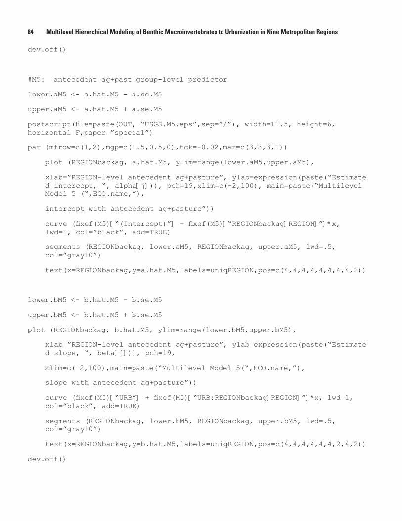
84 Multilevel Hierarchical Modeling of Benthic Macroinvertebrates to Urbanization in Nine Metropolitan Regions
dev.off()
#M5: antecedent ag+past group-level predictor
lower.aM5 <- a.hat.M5 - a.se.M5
upper.aM5 <- a.hat.M5 + a.se.M5
postscript(file=paste(OUT, “USGS.M5.eps”,sep=”/”), width=11.5, height=6, horizontal=F,paper=”special”)
par (mfrow=c(1,2),mgp=c(1.5,0.5,0),tck=-0.02,mar=c(3,3,3,1))
plot (REGIONbackag, a.hat.M5, ylim=range(lower.aM5,upper.aM5),
xlab=”REGION-level antecedent ag+pasture”, ylab=expression(paste(“Estimated intercept, “, alpha[j])), pch=19,xlim=c(-2,100), main=paste(“Multilevel Model 5 (“,ECO.name,”),
intercept with antecedent ag+pasture”))
curve (fixef(M5)[“(Intercept)”] + fixef(M5)[“REGIONbackag[REGION]”]*x, lwd=1, col=”black”, add=TRUE)
segments (REGIONbackag, lower.aM5, REGIONbackag, upper.aM5, lwd=.5, col=”gray10”)
text(x=REGIONbackag,y=a.hat.M5,labels=uniqREGION,pos=c(4,4,4,4,4,4,4,4,2))
lower.bM5 <- b.hat.M5 - b.se.M5
upper.bM5 <- b.hat.M5 + b.se.M5
plot (REGIONbackag, b.hat.M5, ylim=range(lower.bM5,upper.bM5),
xlab=”REGION-level antecedent ag+pasture”, ylab=expression(paste(“Estimated slope, “, beta[j])), pch=19,
xlim=c(-2,100),main=paste(“Multilevel Model 5(“,ECO.name,”),
slope with antecedent ag+pasture”))
curve (fixef(M5)[“URB”] + fixef(M5)[“URB:REGIONbackag[REGION]”]*x, lwd=1, col=”black”, add=TRUE)
segments (REGIONbackag, lower.bM5, REGIONbackag, upper.bM5, lwd=.5, col=”gray10”)
text(x=REGIONbackag,y=b.hat.M5,labels=uniqREGION,pos=c(4,4,4,4,4,4,2,4,2))
dev.off()

Appendix 85
#M6: categorical ag, precip REGION-level predictor
lower.aM6 <- a.hat.M6 - a.se.M6
upper.aM6 <- a.hat.M6 + a.se.M6
postscript(file=paste(OUT, “USGS.M6.eps”,sep=”/”), width=11.5, height=6, horizontal=F,paper=”special”)
par (mfrow=c(1,2),mgp=c(1.5,0.5,0),tck=-0.02,mar=c(3,3,3,1))
plot (REGIONprecip, a.hat.M6, ylim=range(lower.aM6,upper.aM6),
xlab=”REGION-level annual precipitation”, ylab=expression(paste(“Estimated intercept, “, alpha[j])),
pch=19, xlim=c(35,170), col=c(4,4,4,2,2,2,4,4,4), main=paste(“Multilevel Model 6 (“,ECO.name,”),
intercept with ag+grassland and precipitation “))
curve (fixef(M6)[“(Intercept)”] + M6.ranef[[2]][1,1] + fixef(M6)[“REGIONprecip[REGION]”]*x, lwd=1,col=”blue”, add=TRUE)
curve (fixef(M6)[“(Intercept)”] + M6.ranef[[2]][2,1] + fixef(M6)[“REGIONprecip[REGION]”]*x, lwd=1,col=”red”, add=TRUE)
segments (REGIONprecip, lower.aM6, REGIONprecip, upper.aM6, lwd=.5, col=c(4,4,4,2,2,2,4,4,4))
text(x=REGIONprecip,y=a.hat.M6,labels=uniqREGION,pos=c(4,4,4,4,4,4,4,4,4),col=c(4,4,4,2,2,2,4,4,4))
lower.bM6 <- b.hat.M6 - b.se.M6
upper.bM6 <- b.hat.M6 + b.se.M6
plot (REGIONprecip, b.hat.M6, ylim=range(lower.bM6,upper.bM6),
xlab=”REGION-level annual precipitation”, ylab=expression(paste(“Estimated slope, “, beta[j])),pch=19, xlim=c(35,170),col=c(4,4,4,2,2,2,4,4,4),main=paste(“Multilevel Model 6 (“,ECO.name,”),
slope with ag+grassland and precipitation”))
curve (fixef(M6)[“URB”] + M6.ranef[[2]][1,2] + fixef(M6)[“URB:REGIONprecip[REGION]”]*x,lwd=1,col=”blue”, add=TRUE)
curve (fixef(M6)[“URB”] + M6.ranef[[2]][2,2] + fixef(M6)[“URB:REGIONprecip[REGION]”]*x, lwd=1,
col=”red”, add=TRUE)
segments (REGIONprecip, lower.bM6, REGIONprecip, upper.bM6, lwd=.5, col=c(4,4,4,2,2,2,4,4,4))

86 Multilevel Hierarchical Modeling of Benthic Macroinvertebrates to Urbanization in Nine Metropolitan Regions
text(x=REGIONprecip,y=b.hat.M6,labels=uniqREGION,pos=c(4,4,4,4,4,4,4,4,4),col=c(4,4,4,2,2,2,4,4,4))
dev.off()
#M7: categorical ag, temp REGION-level predictor
lower.aM7 <- a.hat.M7 - a.se.M7
upper.aM7 <- a.hat.M7 + a.se.M7
postscript(file=paste(OUT, “USGS.M7.eps”,sep=”/”), width=11.5, height=6, horizontal=F,paper=”special”)
par (mfrow=c(1,2),mgp=c(1.5,0.5,0),tck=-0.02,mar=c(3,3,3,1))
plot (REGIONtemp, a.hat.M7, ylim=range(lower.aM7,upper.aM7),
xlab=”REGION-level annual temperature”, ylab=expression(paste(“Estimated intercept, “, alpha[j])), pch=19,xlim=c(7,20), col=c(4,4,4,2,2,2,4,4,4), main=paste(“Multilevel Model 7 (“,ECO.name,”),
intercept with ag+grassland and temperature”))
curve (fixef(M7)[“(Intercept)”] + M7.ranef[[2]][1,1] + fixef(M7)[“REGIONtemp[REGION]”]*x, lwd=1, col=”blue”, add=TRUE)
curve (fixef(M7)[“(Intercept)”] + M7.ranef[[2]][2,1] + fixef(M7)[“REGIONtemp[REGION]”]*x, lwd=1, col=”red”, add=TRUE)
segments (REGIONtemp, lower.aM7, REGIONtemp, upper.aM7, lwd=.5, col=c(4,4,4,2,2,2,4,4,4))
text(x=REGIONtemp,y=a.hat.M7,labels=uniqREGION,pos=c(4,4,4,4,4,4,4,4,4),col=c(4,4,4,2,2,2,4,4,4))
lower.bM7 <- b.hat.M7 - b.se.M7
upper.bM7 <- b.hat.M7 + b.se.M7
plot (REGIONtemp, b.hat.M7, ylim=range(lower.bM7,upper.bM7),
xlab=”REGION-level annual temperature”, ylab=expression(paste(“Estimated slope, “, beta[j])), pch=19,
xlim=c(7,20),col=c(4,4,4,2,2,2,4,4,4),main=paste(“Multilevel Model 7 (“,ECO.name,”),
slope with ag+grassland and temperature”))
curve (fixef(M7)[“URB”] + M7.ranef[[2]][1,2] + fixef(M7)[“URB:REGIONtemp[REGION]”]*x, lwd=1, col=”blue”, add=TRUE)
curve (fixef(M7)[“URB”] + M7.ranef[[2]][2,2] + fixef(M7)

Appendix 87
[“URB:REGIONtemp[REGION]”]*x, lwd=1, col=”red”, add=TRUE)
segments (REGIONtemp, lower.bM7, REGIONtemp, upper.bM7, lwd=.5, col=c(4,4,4,2,2,2,4,4,4))
text(x=REGIONtemp,y=b.hat.M7,labels=uniqREGION,pos=c(4,4,4,4,4,4,4,4,4),col=c(4,4,4,2,2,2,4,4,4))
dev.off()
#M8: categorical ag, temp REGION-level predictor
lower.aM8 <- a.hat.M8 - a.se.M8
upper.aM8 <- a.hat.M8 + a.se.M8
postscript(file=paste(OUT, “USGS.M8.eps”,sep=”/”), width=11.5, height=6, horizontal=F,paper=”special”)
par (mfrow=c(1,2),mgp=c(1.5,0.5,0),tck=-0.02,mar=c(3,3,3,1))
plot (REGIONtemp, a.hat.M8, ylim=range(lower.aM8,upper.aM8),
xlab=”REGION-level annual temperature”, ylab=expression(paste(“Estimated intercept, “, alpha[j])), pch=19,xlim=c(7,20), col=c(4,4,4,2,2,2,4,4,4), main=paste(“Multilevel Model 8 (“,ECO.name,”),
intercept with ag+grassland and temperature”))
curve (fixef(M8)[“(Intercept)”] + M8.ranef[[2]][1,1] + fixef(M8)[“REGIONtemp[REGION]”]*x, lwd=1, col=”blue”, add=TRUE)
curve (fixef(M8)[“(Intercept)”] + M8.ranef[[2]][2,1] + fixef(M8)[“REGIONtemp[REGION]”]*x, lwd=1, col=”red”, add=TRUE)
segments (REGIONtemp, lower.aM8, REGIONtemp, upper.aM8, lwd=.5, col=c(4,4,4,2,2,2,4,4,4))
text(x=REGIONtemp,y=a.hat.M8,labels=uniqREGION,pos=c(4,2,4,4,4,4,4,4,4),col=c(4,4,4,2,2,2,4,4,4))
lower.bM8 <- b.hat.M8 - b.se.M8
upper.bM8 <- b.hat.M8 + b.se.M8
plot (REGIONprecip, b.hat.M8, ylim=range(lower.bM8,upper.bM8),
xlab=”REGION-level annual precipitation”, ylab=expression(paste(“Estimated slope, “, beta[j])), pch=19, xlim=c(35,170),col=c(4,4,4,2,2,2,4,4,4),main=paste(“Multilevel Model 8 (“,ECO.name,”),
slope with ag+grassland and precipitation”))
curve (fixef(M8)[“URB”] + M8.ranef[[2]][1,2] + fixef(M8)
88 Multilevel Hierarchical Modeling of Benthic Macroinvertebrates to Urbanization in Nine Metropolitan Regions
[“URB:REGIONprecip[REGION]”]*x, lwd=1, col=”blue”, add=TRUE)
curve (fixef(M8)[“URB”] + M8.ranef[[2]][2,2] + fixef(M8)[“URB:REGIONprecip[REGION]”]*x, lwd=1, col=”red”, add=TRUE)
segments (REGIONprecip, lower.bM8, REGIONprecip, upper.bM8, lwd=.5, col=c(4,4,4,2,2,2,4,4,4))
text(x=REGIONprecip,y=b.hat.M8,labels=uniqREGION,pos=c(4,4,4,4,4,4,4,4,4),col=c(4,4,4,2,2,2,4,4,4))
dev.off()

Prepared by:USGS Enterprise Publishing NetworkRaleigh Publishing Service Center3916 Sunset Ridge RoadRaleigh, NC 27607
For additional information regarding this publication, contact:Thomas F. CuffneyU.S. Geological Survey3916 Sunset Ridge RoadRaleigh, NC 27607phone: 1-919-571-4019email: [email protected]
Or visit the Effects of Urbanization on Stream Ecosystems (EUSE) NAWQA Project Web site at:http://water.usgs.gov/nawqa/urban/

Kashuba and others—M
ultilevel Hierarchical M
odeling of Benthic M
acroinvertebrate Responses to Urbanization in N
ine Metropolitan Regions—
Scientific Investigations Report 2009–5243
Printed on recycled paper