�����������������

Citation: Ahmed, H.O.A.; Yu, Y.;

Wang, Q.; Darwish, M.; Nandi, A.K.

Intelligent Fault Diagnosis

Framework for Modular Multilevel

Converters in HVDC Transmission.

Sensors 2022, 22, 362. https://

doi.org/10.3390/s22010362

Academic Editor: Hossam A. Gabbar

Received: 10 November 2021

Accepted: 31 December 2021

Published: 4 January 2022

Publisher’s Note: MDPI stays neutral

with regard to jurisdictional claims in

published maps and institutional affil-

iations.

Copyright: © 2022 by the authors.

Licensee MDPI, Basel, Switzerland.

This article is an open access article

distributed under the terms and

conditions of the Creative Commons

Attribution (CC BY) license (https://

creativecommons.org/licenses/by/

4.0/).

sensors

Article

Intelligent Fault Diagnosis Framework for Modular MultilevelConverters in HVDC TransmissionHosameldin O. A. Ahmed 1, Yuexiao Yu 1,2, Qinghua Wang 1,3, Mohamed Darwish 1 and Asoke K. Nandi 1,4,*

1 Department of Electronic and Electrical Engineering, Brunel University London, Uxbridge UB8 3PH, UK;hosameldin.ahmed3@brunel.ac.uk (H.O.A.A.); yuyuexiao333@hotmail.com (Y.Y.); wqhhuazi@163.com (Q.W.);Mohamed.darwish@brunel.ac.uk (M.D.)

2 State Grid Sichuan Electric Power Research Institute of China, Chengdu 610094, China3 School of Mechatronic Engineering, Xi’an Technological University, Xi’an 710021, China4 Visiting Professor, School of Mechanical Engineering, Xi’an Jiaotong University, Xi’an 710049, China* Correspondence: asoke.nandi@brunel.ac.uk

Abstract: Open circuit failure mode in insulated-gate bipolar transistors (IGBT) is one of the mostcommon faults in modular multilevel converters (MMCs). Several techniques for MMC fault diagno-sis based on threshold parameters have been proposed, but very few studies have considered artificialintelligence (AI) techniques. Using thresholds has the difficulty of selecting suitable threshold valuesfor different operating conditions. In addition, very little attention has been paid to the importanceof developing fast and accurate techniques for the real-life application of open-circuit failures ofIGBT fault diagnosis. To achieve high classification accuracy and reduced computation time, a faultdiagnosis framework with a combination of the AC-side three-phase current, and the upper andlower bridges’ currents of the MMCs to automatically classify health conditions of MMCs is proposed.In this framework, the principal component analysis (PCA) is used for feature extraction. Then,two classification algorithms—multiclass support vector machine (SVM) based on error-correctingoutput codes (ECOC) and multinomial logistic regression (MLR)—are used for classification. Theeffectiveness of the proposed framework is validated by a two-terminal simulation model of the MMC-high-voltage direct current (HVDC) transmission power system using PSCAD/EMTDC software.The simulation results demonstrate that the proposed framework is highly effective in diagnosingthe health conditions of MMCs compared to recently published results.

Keywords: MMC-HVDC; fault detection; fault classification; principal component analysis (PCA);multiclass support vector machine (SVM); multinomial logistic regression (MLR)

1. Introduction

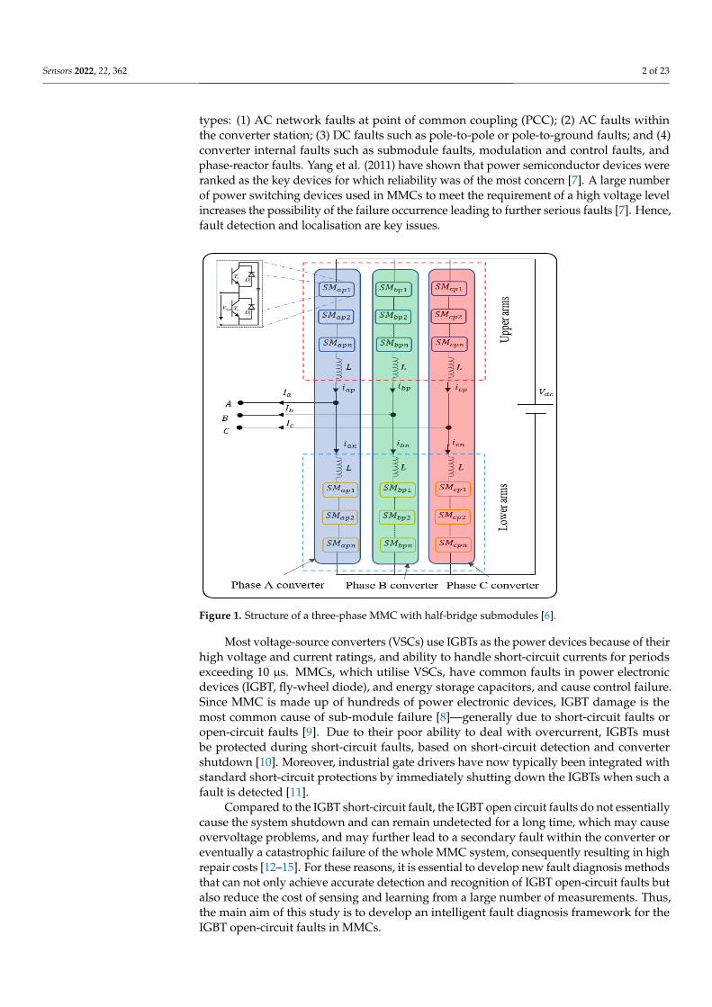
MMCs in HVDC transmission systems offer high voltage, high efficiency, and highquality of AC voltage [1–3]. MMC technology was first introduced by Marquardt [4]in 2001. Recently, it has been implemented by key manufacturers of HVDC equipmentand has shown obvious benefits compared with line communicating converters (LCC)based HVDC. The MMCs are essentially constructed by linking several arms to createa three-phase converter. Each arm is created by several series-connected sub-modulesbuilt with controllable semiconductor devices such as IGBTs, diodes, and capacitors. Inseries with each arm, an inductor is added to smooth the current. Based on how the armsare connected, different MMC structures can be developed [5]. Of these, the double-starstructure is the most applied topology. Figure 1 illustrates a typical structure of a DC tothree-phase AC MMC system with n matching submodules (SMs) in each arm of the upperand lower sides of the converters. Each SM is a half-bridge circuit with two IGBTs and onecapacitor [6]. Condition classification of MMCs can avoid further substantial failures in theMMC system. Recently, there is an increasing interest in fault detection and localisationof MMC-based HVDC converters. Generally, the fault types can be put into four main

Sensors 2022, 22, 362. https://doi.org/10.3390/s22010362 https://www.mdpi.com/journal/sensors

Sensors 2022, 22, 362 2 of 23

types: (1) AC network faults at point of common coupling (PCC); (2) AC faults withinthe converter station; (3) DC faults such as pole-to-pole or pole-to-ground faults; and (4)converter internal faults such as submodule faults, modulation and control faults, andphase-reactor faults. Yang et al. (2011) have shown that power semiconductor devices wereranked as the key devices for which reliability was of the most concern [7]. A large numberof power switching devices used in MMCs to meet the requirement of a high voltage levelincreases the possibility of the failure occurrence leading to further serious faults [7]. Hence,fault detection and localisation are key issues.

Sensors 2022, 22, x FOR PEER REVIEW 2 of 24

system. Recently, there is an increasing interest in fault detection and localisation of MMC-based HVDC converters. Generally, the fault types can be put into four main types: (1) AC network faults at point of common coupling (PCC); (2) AC faults within the con-verter station; (3) DC faults such as pole-to-pole or pole-to-ground faults; and (4) converter internal faults such as submodule faults, modulation and control faults, and phase-reactor faults. Yang et al. (2011) have shown that power semiconductor devices were ranked as the key devices for which reliability was of the most concern [7]. A large number of power switching devices used in MMCs to meet the requirement of a high voltage level increases the possibility of the failure occurrence leading to further serious faults [7]. Hence, fault detection and localisation are key issues.

Figure 1. Structure of a three-phase MMC with half-bridge submodules [6].

Most voltage-source converters (VSCs) use IGBTs as the power devices because of their high voltage and current ratings, and ability to handle short-circuit currents for pe-riods exceeding 10 μs. MMCs, which utilise VSCs, have common faults in power elec-tronic devices (IGBT, fly-wheel diode), and energy storage capacitors, and cause control failure. Since MMC is made up of hundreds of power electronic devices, IGBT damage is the most common cause of sub-module failure [8]—generally due to short-circuit faults or open-circuit faults [9]. Due to their poor ability to deal with overcurrent, IGBTs must be protected during short-circuit faults, based on short-circuit detection and converter shut-down [10]. Moreover, industrial gate drivers have now typically been integrated with standard short-circuit protections by immediately shutting down the IGBTs when such a fault is detected [11].

Compared to the IGBT short-circuit fault, the IGBT open circuit faults do not essen-tially cause the system shutdown and can remain undetected for a long time, which may cause overvoltage problems, and may further lead to a secondary fault within the con-verter or eventually a catastrophic failure of the whole MMC system, consequently result-ing in high repair costs [12–15]. For these reasons, it is essential to develop new fault di-agnosis methods that can not only achieve accurate detection and recognition of IGBT

Figure 1. Structure of a three-phase MMC with half-bridge submodules [6].

Most voltage-source converters (VSCs) use IGBTs as the power devices because of theirhigh voltage and current ratings, and ability to handle short-circuit currents for periodsexceeding 10 µs. MMCs, which utilise VSCs, have common faults in power electronicdevices (IGBT, fly-wheel diode), and energy storage capacitors, and cause control failure.Since MMC is made up of hundreds of power electronic devices, IGBT damage is themost common cause of sub-module failure [8]—generally due to short-circuit faults oropen-circuit faults [9]. Due to their poor ability to deal with overcurrent, IGBTs mustbe protected during short-circuit faults, based on short-circuit detection and convertershutdown [10]. Moreover, industrial gate drivers have now typically been integrated withstandard short-circuit protections by immediately shutting down the IGBTs when such afault is detected [11].

Compared to the IGBT short-circuit fault, the IGBT open circuit faults do not essentiallycause the system shutdown and can remain undetected for a long time, which may causeovervoltage problems, and may further lead to a secondary fault within the converter oreventually a catastrophic failure of the whole MMC system, consequently resulting in highrepair costs [12–15]. For these reasons, it is essential to develop new fault diagnosis methodsthat can not only achieve accurate detection and recognition of IGBT open-circuit faults butalso reduce the cost of sensing and learning from a large number of measurements. Thus,the main aim of this study is to develop an intelligent fault diagnosis framework for theIGBT open-circuit faults in MMCs.

Sensors 2022, 22, 362 3 of 23

Conventional multilevel converter fault diagnosis has many techniques to deal withfault detection and localisation [16–20]. For instance, Khomfoi and Tolbert [16] proposed afault diagnosis and reconfiguration technique for a cascaded H-bridge multilevel inverterdrive using principal component analysis (PCA) and neural network (NN). In this method,the genetic algorithm is used to select valuable principal components. Simulation andexperimental results showed that their method can detect fault type, fault location, andreconfiguration. Song and Huang [17] proposed a fault-tolerant strategy using H-bridgebuilding block (HBBB) redundancy in cascaded H-bridge multilevel converter (CHMC)-based static synchronous compensator (STATCOM). In this strategy, the fault identificationis based on the operator analysis. Simulation and experimental results based on switch-voltage sensed signals appear to validate their method. Sedghi et al. [18] introduced amethod for a cascaded H-bridge fault diagnosis using histogram analysis and NN. In thismethod, the output voltage is used to detect fault type and their locations. Similarly, Jianget al. [19] proposed a method for a cascaded H-bridge inverter fault diagnosis using discreteFourier transform (DFT) and NN. In this method, the output voltage is used as a diagnosticsignal. Lezana et al. [20] proposed a method for cell fault detection using high-frequencyharmonic analysis in a cascaded multicell converter using one voltage measurement peroutput phase. Furthermore, Yazdani et al. [21] introduced a method for multilevel cascadedconverter STATCOM fault detection and mitigation using output phase voltages. Theperformance of this method is validated using PSCAD/EMDTC simulation. Moreover,Wang et al. [22] presented a strategy for multilevel inverter fault diagnosis based on PCAand multiclass relevance vector machine (mRVM). In this strategy, first, the output voltageis used as a diagnostic signal that is pre-processed using a fast Fourier transform (FFT).Then, the PCA is used to extract fault signatures from the sensed output voltage. Withthese extracted features, an mRVM model is used to classify fault types.

Even though the efficiency of these methods and many more in fault diagnosis ofconventional multilevel converters has been validated in many studies, they cannot beused directly for diagnosing a fault in the MMC system owing to differences in structureand operating principle of MMC and conventional multilevel converters [23]. Hence, otherfault diagnosis strategies have been proposed for MMCs. For example, Shao et al. [24]introduced a fault detection method for MMC using a sliding mode observer (SMO) andswitching model of a half-bridge. However, the accuracy of measurements may limitits applications. A fault detection and isolation method for open-circuit faults of powersemiconductor devices in an MMC based on SMO for the circulating current in and MMCwas proposed [25]. Moreover, the detection and location of MMCs’ open-circuit faultusing extended state observer (ESO) has been introduced using differences between thetheoretical and observed full arm voltages [23]. A fault identification method [26] based onwavelet analysis and NN has been proposed. Jiao et al. [27] presented a method for MMCfault diagnosis using the firefly algorithm optimised support vector machine (FA-SVM),in which FFT-PCA is used to extract features from the voltage signal of a three-phase ACside under the open-circuit fault of IGBT. Kiranyaz et al. [28] proposed a real-time systemfor early fault detection and identification using adaptive one-dimensional convolutionalNN. Furthermore, Li et al. introduced a method for fault diagnosis and location for MMCwith the open-circuit fault in SM. In this technique, based on the data character of the basicprinciple of the MMC in a normal or open-circuit fault condition, a mixed kernel supporttensor machine (MKSTM) is offered to dispose of these tensor data [29]. Chen et al. [30]proposed a validation method for the simulation model of a power system integratedwith the internet of things that can process high-dimensional simulation data and provideevidence for model error location. The method consists of two main parts. First, a featureextraction method for multivariate time series using factor analysis and modified adaptiveProny method. Second, a validation model based on the similarity evaluation is established.The validation discussed in this paper identifies the model errors and their locations, whichcan be used to improve the simulation model against the practical/acknowledged system.The method is verified by an application to the MMC-HVDC model in PSASP [30]. Yang

Sensors 2022, 22, 362 4 of 23

et al. proposed two SM failure detection and location techniques, namely, a clusteringalgorithm (CA)-based technique and a calculated capacitance (CC)-based technique. Inthe proposed CA-based method, the K-means clustering algorithm is employed to detectand locate the faulty SMs with open-switch failures through identifying the pattern of 2-Dtrajectories of the SM characteristic variables. The proposed CC-based method is based onthe calculation and comparison of a physical component parameter—namely, the nominalSM capacitance—and is capable of failure detection, location, and classification within onestage [31].

Recently, Huai et al. [32] introduced a single-ended fault location technique with vari-ational mode decomposition (VMD) method and novel parameter optimization scheme us-ing traveling wave (TW) that could be used as an alternative backup plan for communication-based fault location methods. In this method, the VMD is utilised to extract fault featuresfor fault location estimation, which is further improved by using singular entropy-basedparameter optimization. The continuous TW arrivals can be reflected via the most sin-gular IMF under the optimized VMD [32]. Han et al. [33] presented a fault diagnosistechnique based on short-time wavelet entropy integrating the LSTM and the SVM. Inthis technique, the short-time wavelet entropy is used to extract the fault information,then the LSTM process theses information, and finally the output of the LSTM is usedas input of the SVM to obtain the fault diagnosis result [33]. Xing et al. [34] proposeda machine learning-based detection and location method for open-circuit fault. In thismethod, sliding window and feature extraction were used to construct the dataset, whichwas then used to train a model based on multivariate Gaussian distribution for anomalydetection [34]. Ye et al. [35] introduced a technique for fault location of MMC-HVDC usingwavelet transform and deep belief network (DBN). In this technique, first, the wavelettransform is used to decompose the original single pole ground fault voltage waveform,and then the computed high frequency and low-frequency components were used to traindifferent DBN models for fault location estimating [35]. Shen et al. [36] presented a faultdiagnosis method for the IGBT open-circuit faults of different MMC SMs have similar char-acteristics using weighted-amplitude permutation entropy (WAPE), DS evidence fusiontheory, and the LSTM techniques [36]. Ke et al. [37] proposed a fault diagnosis techniquefor MMC based on the synchro-squeezing transform (SST) and genetic algorithm optimizeddeep convolution neural network (GA-DCNN). In this technique, first, the time-frequencyrepresentations (TFRs) of the raw signals which are synthesized by AC, and the innercirculating current of the MMC are calculated with SST. Then, DCNN is employed to learnthe underlying features from the TFRs. The genetic algorithm is used to optimize the keyhyperparameters of the DCNN while batch normalization, dropout, and data augmentationtechnologies are investigated to prevent the DCNN model from overfitting and improvethe performance of the model [37]. More recently, Guo et al. proposed a fault diagnosisframework for MMC using temporal convolutional network (TCN) integrating adaptivechirp mode decomposition (ACMD) and silhouette coefficient (SC). In this technique, first,the ACMD is used to extract and reconstruct signal components from the original signal.Then, SC is used to characterize the importance of each component. Finally, the TCN modelwas employed to automatically extract features from the signal components and providethe classification results [38].

Various HVDC open-circuit fault diagnosis-based studies rely on measurements col-lected from voltage sensors [11,39,40] or both voltage and current sensors [26,41–43] withinthe IGBT modules. In [39], a sensor-less current measurement technique is used. It is mainlybased on measuring the instantaneous sub-modules capacitor voltages with the aim tosuppress the circulating second harmonic current rather than detecting an open-circuit fault.In [40], a reduced number of voltage measuring techniques are used, but an individualvoltage sensor is still needed for each IGBT module. In [11], a method based on the theoret-ical assumption that all measurements are available and are fed to a MATLAB/Simulinkmodel is used. Reference [41] is based on fault diagnosis techniques using both voltage andcurrent sensors. Reference [26] can accurately locate the bridge arm of the faulty submodule

Sensors 2022, 22, 362 5 of 23

but cannot locate the specific sub-module. Reference [42] has the limitation of failing toidentify how many IGBTs failed when multiple faults occur simultaneously. Reference [43]uses excessive current measurements in each arm and the voltage measurements acrosseach submodule. Certainly, there will be huge advantages if a minimum number of onlycurrent sensors are used to detect faults with high accuracy and reduced computation time.This is covered in our paper.

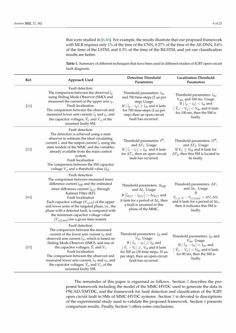
Table 1 records different techniques used for IGBT open circuit fault detection andlocalisation [24,42,44,45], based on threshold parameters. These have difficulties in settingcorrect threshold values for different operating conditions. In contrast, AI-based techniquescan automatically develop a model and improve the accuracy of fault diagnosis. Here, thefault diagnosis of the IGBT open circuit in SMs is studied to overcome the aforementionedproblems and achieve high fault classification accuracy with fewer sensors and reducedcomputational time.

We propose an intelligent diagnosis framework for MMCs faults using machinelearning-based technique and combined information of current sensors to automaticallyrecognise the open-circuit failures of IGBT in MMCs. The contributions of this paper are asfollows:

a. The proposed intelligent fault diagnosis framework utilises only current sensor datafor fault diagnosis. This study achieves high accuracy of fault diagnosis using onlycurrent sensors and AI-based techniques.

b. We combine the measured current data of the AC-side three-phase current and of theupper bridge and lower bridge of each three phases to form a vector of features thatrepresent the current health condition of MMCs.

c. Our proposed framework reduces measured current data using PCA that linearlymaps the current data into a lower-dimensional space of principal components.

d. For fault classification, multiclass SVM based on error-correcting output codes(ECOC) and multinomial logistic regression (MLR) algorithms are used with thelearned feature vector to achieve improved classification accuracy and reducedcomputation time.

e. Compared to recently published results that are based on machine learning tech-niques, our proposed method is faster and yet achieves competitive, if not better,classification accuracies of open-circuit failures of IGBT fault diagnosis in MMC-HVDC transmission.

f. The high reduction in the computational time comes from two elements of ourproposed method: (i) using a minimum number of only current sensors; (ii) using thePCA method to select fewer features that can be used for training the classificationalgorithm—i.e., SVM and MLRC algorithms—and for classifying MMC-HVDC healthconditions using the trained classification models.

g. Being able to obtain high classification accuracy while highly reducing the compu-tational time, our proposed method can be used in real implementations of MMC-HVDC fault diagnosis systems.

The use of only current signals of the AC-side three-phase current and the upper bridgeand lower bridge of each three phases for open-circuit fault detection and classification ofMMCs has been investigated in our recently published papers [6,46]. We have conducted aseries of investigations using the same dataset and deep learning methods to identify thefault type. In [6], we discussed autoencoder-based deep neural network (AE-DNN) andconvolutional neural networks (CNNs) methods. In [46], we investigated long short-termmemory (LSTM) neural network methods. In this paper, our proposed framework reducesmeasured current data using PCA that linearly maps the time series data into a lower-dimensional space of principal components that retain most of the variance of the originalmeasurements of the current signals. Then, for fault classification, ECOC-based SVM andMLR algorithms are used with the learned feature vector to achieve improved classificationaccuracy and reduced computation time. The experimental results demonstrate that ourproposed framework with MLR is much faster than the CNN, AE-DNN, LSTM, and BiLSTM

Sensors 2022, 22, 362 6 of 23

that were studied in [6,46]. For example, the results illustrate that our proposed frameworkwith MLR requires only 1% of the time of the CNN, 0.27% of the time of the AE-DNN, 0.6%of the time of the LSTM, and 0.3% of the time of the BiLSTM, and yet our classificationresults are better.

Table 1. Summary of different techniques that have been used in different studies of IGBT open-circuitfault diagnosis.

Ref. Approach Used Detection ThresholdParameters

Localisation ThresholdParameters

[24]

Fault detection:The comparison between the observed ipusing Sliding Mode Observer (SMO) andmeasured the current of the upper arm ip.

Fault localisationThe comparison between the observed andmeasured lower arm current, ip and ip, and

the capacitor voltages, Vci and Vci of theassumed faulty SM.

Threshold parameters: Ith,and 700 time-steps (2 µs per

step) Usage:If∣∣ ip − ip

∣∣ ≥ Ith and it lastsfor 700 time-steps (2 µs perstep) then an open-circuit

fault has occurred.

Threshold parameters: Ith,Vthi, and 100 ms. Usage:

If∣∣ ip − ip

∣∣ < Ith and∣∣ Vci −Vci∣∣ < Vthi and it lasts

for 100 ms, then the SM isfaulty.

[42]

Fault detection:The detection is achieved using a state

observer to estimate the ideal circulatingcurrent ic and the output current io using thestate models of the MMC and the variables

already available from the main controlsystem.

Fault localisationThe comparison between the SM capacitor

voltage Vci and a threshold value Uth.

Threshold parameters: Ith,and ∆T1. Usage:

If∣∣ ic − ic

∣∣ > Ith and it lastsfor ∆T1, then an open-circuit

fault has occurred.

Threshold parameters: Uth,and ∆T2. Usage:

If Vci ≥ Uth and it lasts for∆T2, then this SM is located to

be faulty.

[44]

Fault detection:The comparison between measured innerdifference current idiff and the estimated

inner difference current idi f f throughKalman Filter (KF).Fault localisation

Each capacitor voltage (Vc,p,N) of the upperand lower arms of the targeted phase, i.e., thephase with a detected fault, is compared with

the minimum capacitor voltage value(Vc(t),min) for a given time instant.

Threshold parameters: ∆idiffand ∆ti. Usage:

If∣∣∣idi f f − idi f f

∣∣∣ > ∆idi f f andit lasts for a period of ∆ti, then

a fault is assumed in thisphase of the MMC.

Threshold parameters: ∆Vcand ∆tv. Usage:

IfVc, p, N −Vc(t),min > ∆Vc ∆Vcand it lasts for a period of ∆tv,

then it indicates this SM isfaulty.

[45]

Fault detection:The comparison between the measuredcurrent of the lower arm current iN and

observed arm current iN , which is based onSliding Mode Observer (SMO), and one of

the capacitor voltages, Vc and Vc.Fault localisation

The comparison between the observed andmeasured lower arm current, iN and iN, and

the capacitor voltages, Vci and Vci of theassumed faulty SM.

Threshold parameters: Ith andVth. Usage:

If∣∣ iN − iN

∣∣ ≥ Ith and∣∣ Vc −Vc∣∣ ≥, Vth and it lasts

for 500 µs (50 time-steps, 10 µsper step), then an open-circuit

fault has occurred.

Threshold parameters: Ith andVthi. Usage:

If∣∣ iN − iN

∣∣ < Ith, and∣∣ Vci −Vci∣∣ < Vthi and it lasts

for 80 ms, then the SM isfaulty.

The remainder of this paper is organised as follows. Section 2 describes the pro-posed framework including the model of the MMC-HVDC used to generate the data inPSCAD/EMTDC, and the framework for fault detection and classification of the IGBTopen circuit fault in SMs of MMC-HVDC systems. Section 3 is devoted to descriptionsof the experimental study used to validate the proposed framework. Section 4 presentscomparison results. Finally, Section 5 offers some conclusions.

Sensors 2022, 22, 362 7 of 23

2. Proposed Framework2.1. Data Modeling

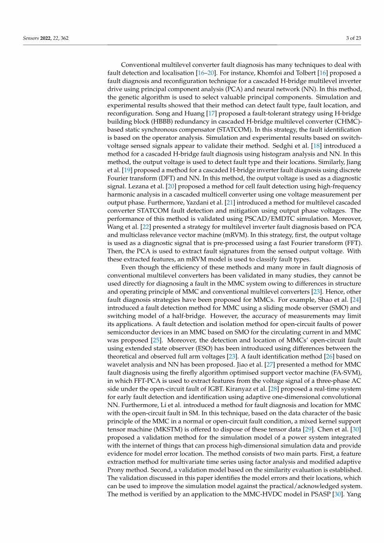
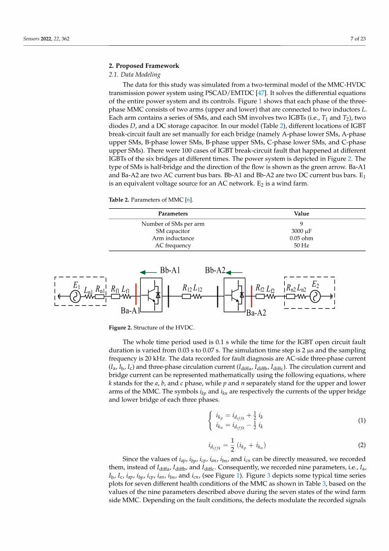
The data for this study was simulated from a two-terminal model of the MMC-HVDCtransmission power system using PSCAD/EMTDC [47]. It solves the differential equationsof the entire power system and its controls. Figure 1 shows that each phase of the three-phase MMC consists of two arms (upper and lower) that are connected to two inductors L.Each arm contains a series of SMs, and each SM involves two IGBTs (i.e., T1 and T2), twodiodes D, and a DC storage capacitor. In our model (Table 2), different locations of IGBTbreak-circuit fault are set manually for each bridge (namely A-phase lower SMs, A-phaseupper SMs, B-phase lower SMs, B-phase upper SMs, C-phase lower SMs, and C-phaseupper SMs). There were 100 cases of IGBT break-circuit fault that happened at differentIGBTs of the six bridges at different times. The power system is depicted in Figure 2. Thetype of SMs is half-bridge and the direction of the flow is shown as the green arrow. Ba-A1and Ba-A2 are two AC current bus bars. Bb-A1 and Bb-A2 are two DC current bus bars. E1is an equivalent voltage source for an AC network. E2 is a wind farm.

Table 2. Parameters of MMC [6].

Parameters Value

Number of SMs per arm 9SM capacitor 3000 µF

Arm inductance 0.05 ohmAC frequency 50 Hz

Sensors 2022, 22, x FOR PEER REVIEW 7 of 24

short-term memory (LSTM) neural network methods. In this paper, our proposed frame-work reduces measured current data using PCA that linearly maps the time series data into a lower-dimensional space of principal components that retain most of the variance of the original measurements of the current signals. Then, for fault classification, ECOC-based SVM and MLR algorithms are used with the learned feature vector to achieve im-proved classification accuracy and reduced computation time. The experimental results demonstrate that our proposed framework with MLR is much faster than the CNN, AE-DNN, LSTM, and BiLSTM that were studied in [6,46]. For example, the results illustrate that our proposed framework with MLR requires only 1% of the time of the CNN, 0.27% of the time of the AE-DNN, 0.6% of the time of the LSTM, and 0.3% of the time of the BiLSTM, and yet our classification results are better.

The remainder of this paper is organised as follows. Section 2 describes the proposed framework including the model of the MMC-HVDC used to generate the data in PSCAD/EMTDC, and the framework for fault detection and classification of the IGBT open circuit fault in SMs of MMC-HVDC systems. Section 3 is devoted to descriptions of the experimental study used to validate the proposed framework. Section 4 presents com-parison results. Finally, Section 5 offers some conclusions.

2. Proposed Framework 2.1. Data Modeling

The data for this study was simulated from a two-terminal model of the MMC-HVDC transmission power system using PSCAD/EMTDC [47]. It solves the differential equations of the entire power system and its controls. Figure 1 shows that each phase of the three-phase MMC consists of two arms (upper and lower) that are connected to two inductors L. Each arm contains a series of SMs, and each SM involves two IGBTs (i.e., 𝑇 and 𝑇 ), two diodes D, and a DC storage capacitor. In our model (Table 2), different locations of IGBT break-circuit fault are set manually for each bridge (namely A-phase lower SMs, A-phase upper SMs, B-phase lower SMs, B-phase upper SMs, C-phase lower SMs, and C-phase upper SMs). There were 100 cases of IGBT break-circuit fault that happened at dif-ferent IGBTs of the six bridges at different times. The power system is depicted in Figure 2. The type of SMs is half-bridge and the direction of the flow is shown as the green arrow. Ba-A1 and Ba-A2 are two AC current bus bars. Bb-A1 and Bb-A2 are two DC current bus bars. E1 is an equivalent voltage source for an AC network. E2 is a wind farm.

Ba-A1 Ba-A2

Bb-A2Bb-A1

R12 L12 Rf2 Lf2 Rn2Ln2Rf1 Lf1Rn1Ln1E1 E2

Figure 2. Structure of the HVDC.

The whole time period used is 0.1 s while the time for the IGBT open circuit fault duration is varied from 0.03 s to 0.07 s. The simulation time step is 2 μs and the sampling frequency is 20 kHz. The data recorded for fault diagnosis are AC-side three-phase current (Ia, Ib, Ic) and three-phase circulation current (Idiffa, Idiffb, Idiffc). The circulation current and bridge current can be represented mathematically using the following equations, where k stands for the a, b, and c phase, while p and n separately stand for the upper and lower arms of the MMC. The symbols ikp and ikn are respectively the currents of the upper bridge and lower bridge of each three phases.

Figure 2. Structure of the HVDC.

The whole time period used is 0.1 s while the time for the IGBT open circuit faultduration is varied from 0.03 s to 0.07 s. The simulation time step is 2 µs and the samplingfrequency is 20 kHz. The data recorded for fault diagnosis are AC-side three-phase current(Ia, Ib, Ic) and three-phase circulation current (Idiffa, Idiffb, Idiffc). The circulation current andbridge current can be represented mathematically using the following equations, wherek stands for the a, b, and c phase, while p and n separately stand for the upper and lowerarms of the MMC. The symbols ikp and ikn are respectively the currents of the upper bridgeand lower bridge of each three phases.{

ikp = idi f f k+ 1

2 ik

ikn = idi f f k− 1

2 ik(1)

idi f f k=

12(ikp + ikn) (2)

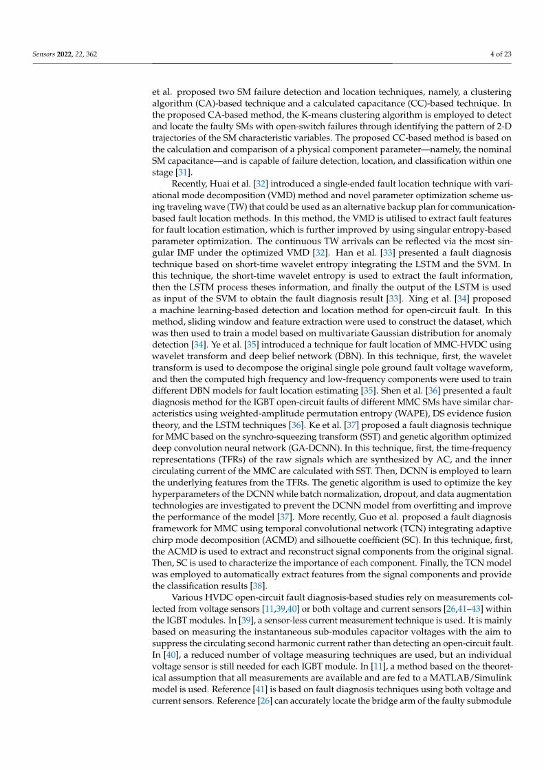
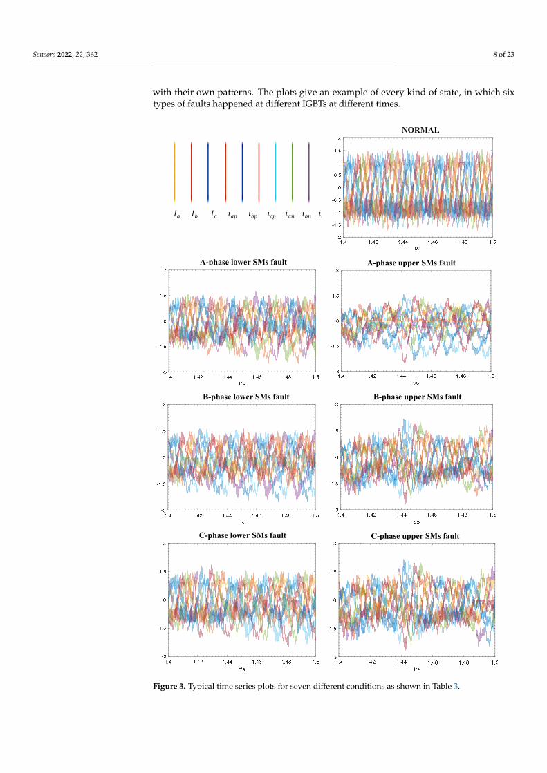
Since the values of iap, ibp, icp, ian, ibn, and icn can be directly measured, we recordedthem, instead of Idiffa, Idiffb, and Idiffc. Consequently, we recorded nine parameters, i.e., Ia,Ib, Ic, iap, ibp, icp, ian, ibn, and icn, (see Figure 1). Figure 3 depicts some typical time seriesplots for seven different health conditions of the MMC as shown in Table 3, based on thevalues of the nine parameters described above during the seven states of the wind farmside MMC. Depending on the fault conditions, the defects modulate the recorded signals

Sensors 2022, 22, 362 8 of 23

with their own patterns. The plots give an example of every kind of state, in which sixtypes of faults happened at different IGBTs at different times.

1

Figure 3. Typical time series plots for seven different conditions as shown in Table 3.

A-phase lower SMs fault A-phase upper SMs fault

B-phase lower SMs fault B-phase upper SMs fault

C-phase lower SMs fault C-phase upper SMs fault

NORMAL

𝐼𝑎 𝐼𝑏 𝐼𝑐 𝑖𝑎𝑝 𝑖𝑏𝑝 𝑖𝑐𝑝 𝑖𝑎𝑛 𝑖𝑏𝑛 𝑖𝑐

Figure 3. Typical time series plots for seven different conditions as shown in Table 3.

Sensors 2022, 22, 362 9 of 23

Table 3. MMC health conditions [6].

Faulty Bridge Label Value

Normal 1A-phase lower SMs 2A-phase upper SMs 3B-phase lower SMs 4B-phase upper SMs 5C-phase lower SMs 6C-phase upper SMs 7

2.2. Description of the Proposed Framework

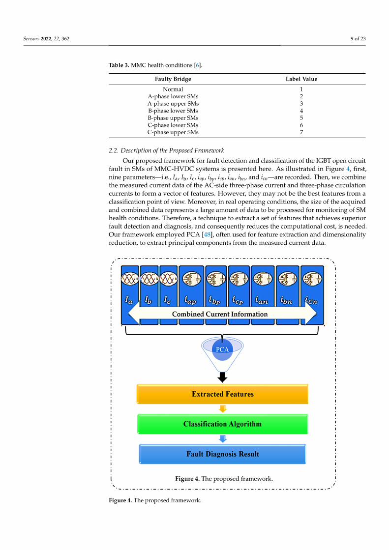
Our proposed framework for fault detection and classification of the IGBT open circuitfault in SMs of MMC-HVDC systems is presented here. As illustrated in Figure 4, first,nine parameters—i.e., Ia, Ib, Ic, iap, ibp, icp, ian, ibn, and icn—are recorded. Then, we combinethe measured current data of the AC-side three-phase current and three-phase circulationcurrents to form a vector of features. However, they may not be the best features from aclassification point of view. Moreover, in real operating conditions, the size of the acquiredand combined data represents a large amount of data to be processed for monitoring of SMhealth conditions. Therefore, a technique to extract a set of features that achieves superiorfault detection and diagnosis, and consequently reduces the computational cost, is needed.Our framework employed PCA [48], often used for feature extraction and dimensionalityreduction, to extract principal components from the measured current data.

Sensors 2022, 22, x FOR PEER REVIEW 10 of 24

2.2. Description of the Proposed Framework Our proposed framework for fault detection and classification of the IGBT open cir-

cuit fault in SMs of MMC-HVDC systems is presented here. As illustrated in Figure 4, first, nine parameters—i.e., Ia, Ib, Ic, iap, ibp, icp, ian, ibn, and icn—are recorded. Then, we combine the measured current data of the AC-side three-phase current and three-phase circulation currents to form a vector of features. However, they may not be the best features from a classification point of view. Moreover, in real operating conditions, the size of the ac-quired and combined data represents a large amount of data to be processed for monitor-ing of SM health conditions. Therefore, a technique to extract a set of features that achieves superior fault detection and diagnosis, and consequently reduces the computational cost, is needed. Our framework employed PCA [48], often used for feature extraction and di-mensionality reduction, to extract principal components from the measured current data.

Figure 4. The proposed framework.

The PCA [48] is used to form a low-dimensional feature vector from the high-dimen-sional combined current data by ignoring the least significant of these components from the PCA. The process of PCA using eigenvector decomposition includes the following steps: First, calculate the mean vector of the combined measured data. Then, compute the covariance matrix of the combined measured data. Finally, obtain the eigenvalues and eigenvectors of the covariance matrix. Suppose that the combined measured dataset 𝑋 = 𝑥 𝑥 … 𝑥 has L observations and N-dimensional space. PCA transforms X to 𝑋 = 𝑥 , 𝑥 , … , 𝑥 in a new 𝑚-dimensional space. The aim is to reduce the dimensionality

Figure 4. The proposed framework.

Sensors 2022, 22, 362 10 of 23

The PCA [48] is used to form a low-dimensional feature vector from the high-dimensionalcombined current data by ignoring the least significant of these components from the PCA.The process of PCA using eigenvector decomposition includes the following steps: First,calculate the mean vector of the combined measured data. Then, compute the covariancematrix of the combined measured data. Finally, obtain the eigenvalues and eigenvectors ofthe covariance matrix. Suppose that the combined measured dataset X = [x1, x2 . . . xL] hasL observations and N-dimensional space. PCA transforms X to X = [ x1, x2, . . . , xL] in anew m-dimensional space. The aim is to reduce the dimensionality from N to m (m� N)of measurements. To calculate the transformation matrix W, PCA utilises eigenvalues andeigenvectors as

λ→V = CX

→V (3)

Here, λ is an eigenvalue,→V is an eigenvector, and CX is the related covariance matrix

of the combined data X, which can be computed by applying the following Equation (4).

CX =1L

L

∑i=1

(xi − x)(xi − x)T (4)

where xi is observation (i) of the combined measured data and x is the mean of the observa-tions, which can be calculated using the equation,

x =1L

L

∑i=1

xi (5)

To reduce the dimensionality of our combined data X by means of PCA using eigen-vector, one ignores the least important components from the principal components, i.e.,columns of V, as

X = WT1 x (6)

Here X ∈ RL x m is the obtained low-dimensional data matrix of our combined data x,and W1 is the projection matrix.

Finally, with these extracted features, SVM-based ECOC and MLR algorithms are usedfor classification.

2.2.1. SVM-Based ECOC

SVM is a supervised learning algorithm that was first proposed for binary classifi-cations [49]. The basic idea of SVM is that it can find the best hyperplane(s) to separatedata from two different classes in such a way that the distance between the two classes,which is called the margin, is maximised. The basic SVM classifier is constructed from asimple linear maximum margin classifier. Briefly, we present the simplified SVM classifieras follows:

With a set of examples of the obtained low-dimensional data of our combined data, i.e.,the selected features from PCA, (X ∈ RL x m) along with their associated class C ∈ RL x 1

such that,X = (x1, c1), (x2, c2), . . . , (xL, cL) (7)

= (xi, ci), , ∀i = 1, 2, . . ., L (8)

Here xi ∈ Rm is an m-dimensional input vector that represents the observation (i) of thelow-dimensional matrix and ci is the associated class label for every i = 1, 2, . . ., L. Assumeci ∈ {+1,−1} for two possible classes ‘NORMAL’ and ‘FAULTY’ conditions, which is abinary classification problem. Binary classification aims to define a function f (x) that cansuccessfully predict the class label ci for an input vector xi by defining a hyperplane, which

Sensors 2022, 22, 362 11 of 23

is also called a boundary, that can separate the examples with the NORMAL class from theexamples with the FAULTY class such that

f (x) = sgn(

wTx + b)

(9)

Here sgn is the sign of(wTx + b

), x is the input vector, w is an m-dimensional vector

that defines the boundary, and b is a scalar. To find the best boundary the following threehypothesizes are defined,

H0 = wTx + b = 0 (10)

H1 = wTx + b = −1 (11)

H2 = wTx + b = +1 (12)

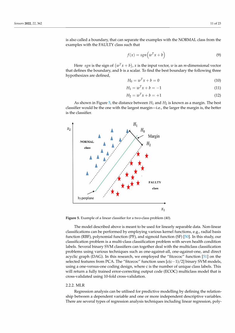
As shown in Figure 5, the distance between H1 and H2 is known as a margin. The bestclassifier would be the one with the largest margin—i.e., the larger the margin is, the betteris the classifier.

2

Figure 5. Example of a linear classifier for a two-class problem (40).

The model described above is meant to be used for linearly separable data. Non-linearclassifications can be performed by employing various kernel functions, e.g., radial basisfunction (RBF), polynomial function (PF), and sigmoid function (SF) [50]. In this study, ourclassification problem is a multi-class classification problem with seven health conditionlabels. Several binary SVM classifiers can together deal with the multiclass classificationproblems using various techniques such as one-against-all, one-against-one, and directacyclic graph (DAG). In this research, we employed the “fitcecoc” function [51] on theselected features from PCA. The “fitcecoc” function uses [c(c−1)/2] binary SVM models,using a one-versus-one coding design, where c is the number of unique class labels. Thiswill return a fully trained error-correcting output code (ECOC) multiclass model that iscross-validated using 10-fold cross-validation.

2.2.2. MLR

Regression analysis can be utilised for predictive modelling by defining the relation-ship between a dependent variable and one or more independent descriptive variables.There are several types of regression analysis techniques including linear regression, poly-

Sensors 2022, 22, 362 12 of 23

nomial regression, logistic regression, etc. Logistic regression (LR) is one of the most widelyused techniques in binary classification problems. Briefly, we describe the LR as follows:

Let a set of examples of the obtained low-dimensional data of our combined data, i.e.,the selected features from PCA, (X ∈ RL x m) along with their associated class C ∈ RL x 1 asdescribed in Equations (7) and (8) above. The LR is a probabilistic discriminative methodthat learns P(c|x) directly from the training where ci ∈ {0, 1} such that

P(c = 1|x ) = h1(x) = g(−θTh

)= 1/(1 + e−θTq) (13)

Here c = 1 is the class, x is the input observation of the obtained low-dimensional data,and g

(−θTh

)is the logistic function. As ∑ P(C) = 1 then P(c = 0|x ) can be calculated as

P(c = 0|x ) = h0(x) = 1− P(c = 1|x ) = 1−(

1/(

1 + e−θT x))

(14)

The likelihood of the parameters of L examples of the data can be calculated as

`(θ) =L

∏i=1

((

g(

θTxi))c(i)

(1− g(

θTxi))

1−c(i)(15)

Here θ = [θ0, θ1, . . . , θi] are the model parameters. The log-likelihood is widely usedand can be computed as

log `(θ) =L

∑i=1

log(((

g(

θTxi))c(i)

(1− g(

θTxi))1−c(i)) (16)

To avoid the overfitting, a regularisation term λ is added the log-likelihood functionsuch that

log `(θ) =L

∑i=1

log(

P(

ci = ck

∣∣∣xi; θ))− λ

2‖ θ ‖2 (17)

The MLR is a linear supervised regression model that generalises the logistic regression(LR) where labels are binary, i.e., c(i) ∈ {0,1} to multi-classification problems that have labels{1, . . . , c} where c is the number of classes. The LR and MLR have been used in machinefault diagnosis [52–55]. We briefly describe the simplified multinomial logistic regressionmodel as follows: in multinomial logistic regression with multi-labels c(i) ∈ {1, . . . , c} theaim is to estimate the probability P(c = c(i) |x) for each value of c(i) = 1 to c, such that

hθ(x) =

P(c = 1|x; θ)P(c = 2|x; θ)

.

.

.P(c = K|x; θ)

=1

∑Kj=1 exp

(θ(j)Tx

)

eθ(1)T x

eθ(2)T x

.

.

.eθ(K)T x

(18)

where θ(1), θ(2) , . . . , θ(K) ∈ Rn are the parameters of the multinomial logistic regressionmodel.

3. Experimental Study

The data used in this study were collected from a two-terminal simulation model ofthe MMC-HVDC transmission power system described in Section 2. Seven conditionsof MMCs status have been recorded. These include one normal condition and six IGBTopen-circuit fault conditions in lower and upper arms of the MMC containing, A-phaselower SMs, A-phase upper SMs, B-phase lower SMs, B-phase upper SMs, C-phase lowerSMs, and C-phase upper SMs faults. A total of 100 examples of each condition were

Sensors 2022, 22, 362 13 of 23

recorded; this gave a total of 700 (100 × 7) raw data files to work with. All the nineparameters—i.e., Ia, Ib, Ic, iap, ibp, icp, ian, ibn, and icn—were recorded to obtain 5001 timesamples. The measurements of these nine parameters were concatenated to form a vectorof samples that represent the current health condition of the MMCs. This gave a total of45,009 (5001 × 9) samples dimension for each vector of health condition. First, experimentswere conducted for testing data of sizes 15% to 50% and 20 trials for each experiment with10-fold cross-validation.

By using PCA on the concatenated measurements and then ignoring all eigenvaluesless than 10−10 of the largest eigenvalue, we obtain 604 principal components, retainingwell over 99% of the total variance of the data. With these learned features, SVM-basedon the ECOC algorithm and MLR algorithm are used for classification. Classificationaccuracies are obtained by averaging the results of twenty trials for each classifier and eachexperiment. Additionally, in each experiment, we have examined the effects of using anormalisation technique in our classification results for both SVM and MLR.

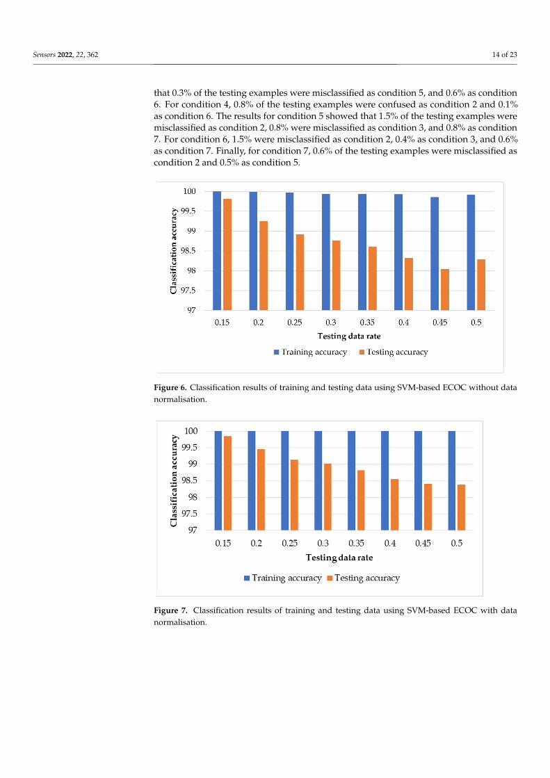
3.1. Results of SVM-Based ECOC without Data Normalisation

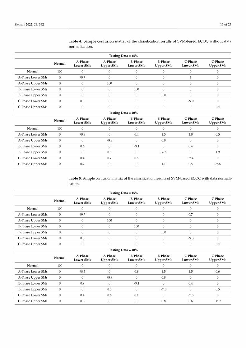
Figure 6 shows the classification results of training and testing data using our frame-work with an SVM-based ECOC classifier without data normalisation. On average, thetesting classification results have high classification accuracies from 99.8% with 15% testingdata to 98.0% with a 45% testing data rate. A possible explanation for these results might bethat the increase in the training data might improve the accuracy of the trained classificationmodel. Table 4 provides a sample confusion matrix of the classification results for eachcondition with testing data of 15% and 40%. As can be seen from Table 4, the recognition ofthe normal condition of the MMCs is 100% with both the 15% and 40% testing data. With15% testing data, our method misclassified none of the testing examples of conditions 1,3, 4, 5, and 7. For condition 2, our method misclassified 0.3% of the testing examples ofcondition 2 as condition 6 and 1% of the testing examples of condition 6 as condition 2.However, with 40% testing data, our method misclassified 1.2% of the testing examples ofcondition 2 as condition 4 (0.6%), condition 6 (0.4%), and condition 7 (0.2%) For condition3, our proposed method misclassified 1.1% of the testing examples as condition 5 (0.3%)and condition 6 (0.7%). For condition 4, 0.9% of the testing examples were misclassified ascondition 2 (0.4%) and condition 6 (0.5%). Results for condition 5 misclassified 3.4% of thetesting examples as condition 2 (1.5%), condition 3 (0.8%), and condition 7 (1.1). Resultsfor condition 6 showed that 1.8% of the testing examples were confused as condition 2,0.4% of the testing examples were misclassified as condition 4, and 0.5% were misclassifiedas condition 7. Finally, 2.4% of the testing examples of condition 7 were misclassified ascondition 2 (0.5%) and condition 5 (1.9%).

3.2. Results of SVM-Based ECOC with Data Normalisation

Figure 7 shows the classification results of training and testing data using our frame-work with the SVM classifier and data normalisation. Overall, the testing classificationresults have high classification accuracies where the minimum accuracy achieved is 98.4%with 50% testing data and maximum accuracy is 99.9% with 15% testing data. This indicatesthat there was a slight improvement in the classification accuracy of SVM-based ECOCwith data normalization compared to the classification results without data normalizationdescribed above. Table 5 shows the sample confusion matrix of the classification resultsfor each health condition with testing data of 15% and 40%. Additionally, the recognitionof the normal healthy condition is 100% with both 15% and 40% of testing data. With15% testing data, there are no misclassifications of conditions 1, 3, 4, 5, and 7. Results forcondition 2 showed that 0.3% of the testing examples were confused as condition 6. Whilefor condition 6, the results revealed that 0.7% of the testing examples were misclassified ascondition 2. With 40% testing data, the recognition accuracy for condition 1—i.e., the nor-mal condition—was 100%. For condition 2, 0.9% of the testing examples were misclassifiedas condition 4, 0.4% as condition 6, and 0.3% as condition 7. Results for condition 3 showed

Sensors 2022, 22, 362 14 of 23

that 0.3% of the testing examples were misclassified as condition 5, and 0.6% as condition6. For condition 4, 0.8% of the testing examples were confused as condition 2 and 0.1%as condition 6. The results for condition 5 showed that 1.5% of the testing examples weremisclassified as condition 2, 0.8% were misclassified as condition 3, and 0.8% as condition7. For condition 6, 1.5% were misclassified as condition 2, 0.4% as condition 3, and 0.6%as condition 7. Finally, for condition 7, 0.6% of the testing examples were misclassified ascondition 2 and 0.5% as condition 5.

Sensors 2022, 22, x FOR PEER REVIEW 14 of 24

well over 99% of the total variance of the data. With these learned features, SVM-based on the ECOC algorithm and MLR algorithm are used for classification. Classification accura-cies are obtained by averaging the results of twenty trials for each classifier and each ex-periment. Additionally, in each experiment, we have examined the effects of using a nor-malisation technique in our classification results for both SVM and MLR.

3.1. Results of SVM-Based ECOC without Data Normalisation Figure 6 shows the classification results of training and testing data using our frame-

work with an SVM-based ECOC classifier without data normalisation. On average, the testing classification results have high classification accuracies from 99.8% with 15% test-ing data to 98.0% with a 45% testing data rate. A possible explanation for these results might be that the increase in the training data might improve the accuracy of the trained classification model. Table 4 provides a sample confusion matrix of the classification re-sults for each condition with testing data of 15% and 40%. As can be seen from Table 4, the recognition of the normal condition of the MMCs is 100% with both the 15% and 40% testing data. With 15% testing data, our method misclassified none of the testing examples of conditions 1, 3, 4, 5, and 7. For condition 2, our method misclassified 0.3% of the testing examples of condition 2 as condition 6 and 1% of the testing examples of condition 6 as condition 2. However, with 40% testing data, our method misclassified 1.2% of the testing examples of condition 2 as condition 4 (0.6%), condition 6 (0.4%), and condition 7 (0.2%) For condition 3, our proposed method misclassified 1.1% of the testing examples as con-dition 5 (0.3%) and condition 6 (0.7%). For condition 4, 0.9% of the testing examples were misclassified as condition 2 (0.4%) and condition 6 (0.5%). Results for condition 5 misclas-sified 3.4% of the testing examples as condition 2 (1.5%), condition 3 (0.8%), and condition 7 (1.1). Results for condition 6 showed that 1.8% of the testing examples were confused as condition 2, 0.4% of the testing examples were misclassified as condition 4, and 0.5% were misclassified as condition 7. Finally, 2.4% of the testing examples of condition 7 were mis-classified as condition 2 (0.5%) and condition 5 (1.9%).

Figure 6. Classification results of training and testing data using SVM-based ECOC without data normalisation.

Figure 6. Classification results of training and testing data using SVM-based ECOC without datanormalisation.

Sensors 2022, 22, x FOR PEER REVIEW 16 of 24

Table 5. Sample confusion matrix of the classification results of SVM-based ECOC with data nor-malisation

Testing Data = 15%

Normal A-Phase Lower SMs

A-Phase Upper SMs

B-Phase Lower SMs

B-Phase Upper SMs

C-Phase Lower SMs

C-Phase Upper SMs

Normal 100 0 0 0 0 0 0 A-Phase Lower SMs 0 99.7 0 0 0 0.7 0 A-Phase Upper SMs 0 0 100 0 0 0 0 B-Phase Lower SMs 0 0 0 100 0 0 0 B-Phase Upper SMs 0 0 0 0 100 0 0 C-Phase Lower SMs 0 0.3 0 0 0 99.3 0 C-Phase Upper SMs 0 0 0 0 0 0 100

Testing Data = 40%

Normal A-Phase Lower SMs

A-Phase Upper SMs

B-Phase Lower SMs

B-Phase Upper SMs

C-Phase Lower SMs

C-Phase Upper SMs

Normal 100 0 0 0 0 0 0 A-Phase Lower SMs 0 98.5 0 0.8 1.5 1.5 0.6 A-Phase Upper SMs 0 0 98.9 0 0.8 0 0 B-Phase Lower SMs 0 0.9 0 99.1 0 0.4 0 B-Phase Upper SMs 0 0 0.5 0 97.0 0 0.5 C-Phase Lower SMs 0 0.4 0.6 0.1 0 97.5 0 C-Phase Upper SMs 0 0.3 0 0 0.8 0.6 98.9

Figure 7. Classification results of training and testing data using SVM-based ECOC with data nor-malisation.

3.3. Results of MLR without Data Normalisation Figure 8 depicts the classification results of training and testing data using our frame-

work with the MLR classifier without data normalisation. Figure 8 indicates that the test-ing results have classification accuracies above 99% for all the rates of testing data used in this study. In particular, classification results from our proposed method with MLR are 99.8% and 99.5% for testing data without normalisation of 15% and 20%, respectively. The least classification accuracy was achieved using testing data of 35% with 99%. Table 6

Figure 7. Classification results of training and testing data using SVM-based ECOC with datanormalisation.

Sensors 2022, 22, 362 15 of 23

Table 4. Sample confusion matrix of the classification results of SVM-based ECOC without datanormalization.

Testing Data = 15%

Normal A-PhaseLower SMs

A-PhaseUpper SMs

B-PhaseLower SMs

B-PhaseUpper SMs

C-PhaseLower SMs

C-PhaseUpper SMs

Normal 100 0 0 0 0 0 0

A-Phase Lower SMs 0 99.7 0 0 0 1 0

A-Phase Upper SMs 0 0 100 0 0 0 0

B-Phase Lower SMs 0 0 0 100 0 0 0

B-Phase Upper SMs 0 0 0 0 100 0 0

C-Phase Lower SMs 0 0.3 0 0 0 99.0 0

C-Phase Upper SMs 0 0 0 0 0 0 100

Testing Data = 40%

Normal A-PhaseLower SMs

A-PhaseUpper SMs

B-PhaseLower SMs

B-PhaseUpper SMs

C-PhaseLower SMs

C-PhaseUpper SMs

Normal 100 0 0 0 0 0 0

A-Phase Lower SMs 0 98.8 0 0.4 1.5 1.8 0.5

A-Phase Upper SMs 0 0 98.8 0 0.8 0 0

B-Phase Lower SMs 0 0.6 0 99.1 0 0.4 0

B-Phase Upper SMs 0 0 0.5 0 96.6 0 1.9

C-Phase Lower SMs 0 0.4 0.7 0.5 0 97.4 0

C-Phase Upper SMs 0 0.2 0 0 1.1 0.5 97.6

Table 5. Sample confusion matrix of the classification results of SVM-based ECOC with data normali-sation.

Testing Data = 15%

Normal A-PhaseLower SMs

A-PhaseUpper SMs

B-PhaseLower SMs

B-PhaseUpper SMs

C-PhaseLower SMs

C-PhaseUpper SMs

Normal 100 0 0 0 0 0 0

A-Phase Lower SMs 0 99.7 0 0 0 0.7 0

A-Phase Upper SMs 0 0 100 0 0 0 0

B-Phase Lower SMs 0 0 0 100 0 0 0

B-Phase Upper SMs 0 0 0 0 100 0 0

C-Phase Lower SMs 0 0.3 0 0 0 99.3 0

C-Phase Upper SMs 0 0 0 0 0 0 100

Testing Data = 40%

Normal A-PhaseLower SMs

A-PhaseUpper SMs

B-PhaseLower SMs

B-PhaseUpper SMs

C-PhaseLower SMs

C-PhaseUpper SMs

Normal 100 0 0 0 0 0 0

A-Phase Lower SMs 0 98.5 0 0.8 1.5 1.5 0.6

A-Phase Upper SMs 0 0 98.9 0 0.8 0 0

B-Phase Lower SMs 0 0.9 0 99.1 0 0.4 0

B-Phase Upper SMs 0 0 0.5 0 97.0 0 0.5

C-Phase Lower SMs 0 0.4 0.6 0.1 0 97.5 0

C-Phase Upper SMs 0 0.3 0 0 0.8 0.6 98.9

Sensors 2022, 22, 362 16 of 23

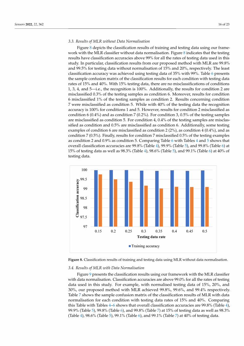
3.3. Results of MLR without Data Normalisation

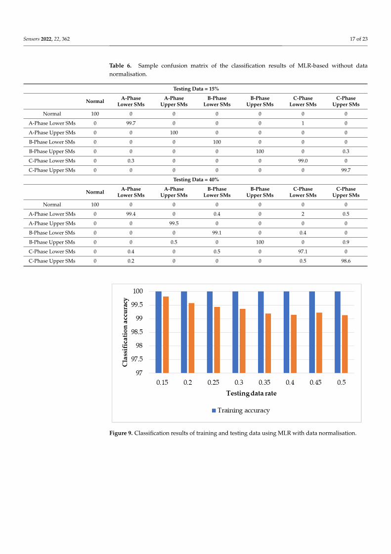
Figure 8 depicts the classification results of training and testing data using our frame-work with the MLR classifier without data normalisation. Figure 8 indicates that the testingresults have classification accuracies above 99% for all the rates of testing data used in thisstudy. In particular, classification results from our proposed method with MLR are 99.8%and 99.5% for testing data without normalisation of 15% and 20%, respectively. The leastclassification accuracy was achieved using testing data of 35% with 99%. Table 6 presentsthe sample confusion matrix of the classification results for each condition with testing datarates of 15% and 40%. With 15% testing data, there are no misclassifications of conditions1, 3, 4, and 5—i.e., the recognition is 100%. Additionally, the results for condition 2 aremisclassified 0.3% of the testing samples as condition 6. Moreover, results for condition6 misclassified 1% of the testing samples as condition 2. Results concerning condition7 were misclassified as condition 5. While with 40% of the testing data the recognitionaccuracy is 100% for conditions 1 and 5. However, results for condition 2 misclassified ascondition 6 (0.4%) and as condition 7 (0.2%). For condition 3, 0.5% of the testing samplesare misclassified as condition 5. For condition 4, 0.4% of the testing samples are misclas-sified as condition and 0.5% are misclassified as condition 6. Additionally, some testingexamples of condition 6 are misclassified as condition 2 (2%), as condition 4 (0.4%), and ascondition 7 (0.5%). Finally, results for condition 7 misclassified 0.5% of the testing examplesas condition 2 and 0.9% as condition 5. Comparing Table 6 with Tables 4 and 5 shows thatoverall classification accuracies are 99.8% (Table 4), 99.9% (Table 5), and 99.8% (Table 6) at15% of testing data as well as 98.3% (Table 4), 98.6% (Table 5), and 99.1% (Table 6) at 40% oftesting data.

Sensors 2022, 22, x FOR PEER REVIEW 18 of 24

Figure 8. Classification results of training and testing data using MLR without data normalisation.

3.4. Results of MLR with Data Normalisation Figure 9 presents the classification results using our framework with the MLR classi-

fier with data normalisation. Classification accuracies are above 99.0% for all the rates of testing data used in this study. For example, with normalised testing data of 15%, 20%, and 30%, our proposed method with MLR achieved 99.8%, 99.6%, and 99.4% respectively. Table 7 shows the sample confusion matrix of the classification results of MLR with data normalisation for each condition with testing data rates of 15% and 40%. Comparing this Table with Tables 4–6 shows that overall classification accuracies are 99.8% (Table 4), 99.9% (Table 5), 99.8% (Table 6), and 99.8% (Table 7) at 15% of testing data as well as 98.3% (Table 4), 98.6% (Table 5), 99.1% (Table 6), and 99.1% (Table 7) at 40% of testing data.

Figure 9. Classification results of training and testing data using MLR with data normalisation.

Figure 8. Classification results of training and testing data using MLR without data normalisation.

3.4. Results of MLR with Data Normalisation

Figure 9 presents the classification results using our framework with the MLR classifierwith data normalisation. Classification accuracies are above 99.0% for all the rates of testingdata used in this study. For example, with normalised testing data of 15%, 20%, and30%, our proposed method with MLR achieved 99.8%, 99.6%, and 99.4% respectively.Table 7 shows the sample confusion matrix of the classification results of MLR with datanormalisation for each condition with testing data rates of 15% and 40%. Comparingthis Table with Tables 4–6 shows that overall classification accuracies are 99.8% (Table 4),99.9% (Table 5), 99.8% (Table 6), and 99.8% (Table 7) at 15% of testing data as well as 98.3%(Table 4), 98.6% (Table 5), 99.1% (Table 6), and 99.1% (Table 7) at 40% of testing data.

Sensors 2022, 22, 362 17 of 23

Table 6. Sample confusion matrix of the classification results of MLR-based without datanormalisation.

Testing Data = 15%

Normal A-PhaseLower SMs

A-PhaseUpper SMs

B-PhaseLower SMs

B-PhaseUpper SMs

C-PhaseLower SMs

C-PhaseUpper SMs

Normal 100 0 0 0 0 0 0

A-Phase Lower SMs 0 99.7 0 0 0 1 0

A-Phase Upper SMs 0 0 100 0 0 0 0

B-Phase Lower SMs 0 0 0 100 0 0 0

B-Phase Upper SMs 0 0 0 0 100 0 0.3

C-Phase Lower SMs 0 0.3 0 0 0 99.0 0

C-Phase Upper SMs 0 0 0 0 0 0 99.7

Testing Data = 40%

Normal A-PhaseLower SMs

A-PhaseUpper SMs

B-PhaseLower SMs

B-PhaseUpper SMs

C-PhaseLower SMs

C-PhaseUpper SMs

Normal 100 0 0 0 0 0 0

A-Phase Lower SMs 0 99.4 0 0.4 0 2 0.5

A-Phase Upper SMs 0 0 99.5 0 0 0 0

B-Phase Lower SMs 0 0 0 99.1 0 0.4 0

B-Phase Upper SMs 0 0 0.5 0 100 0 0.9

C-Phase Lower SMs 0 0.4 0 0.5 0 97.1 0

C-Phase Upper SMs 0 0.2 0 0 0 0.5 98.6

Sensors 2022, 22, x FOR PEER REVIEW 18 of 24

Figure 8. Classification results of training and testing data using MLR without data normalisation.

3.4. Results of MLR with Data Normalisation Figure 9 presents the classification results using our framework with the MLR classi-

fier with data normalisation. Classification accuracies are above 99.0% for all the rates of testing data used in this study. For example, with normalised testing data of 15%, 20%, and 30%, our proposed method with MLR achieved 99.8%, 99.6%, and 99.4% respectively. Table 7 shows the sample confusion matrix of the classification results of MLR with data normalisation for each condition with testing data rates of 15% and 40%. Comparing this Table with Tables 4–6 shows that overall classification accuracies are 99.8% (Table 4), 99.9% (Table 5), 99.8% (Table 6), and 99.8% (Table 7) at 15% of testing data as well as 98.3% (Table 4), 98.6% (Table 5), 99.1% (Table 6), and 99.1% (Table 7) at 40% of testing data.

Figure 9. Classification results of training and testing data using MLR with data normalisation.

Figure 9. Classification results of training and testing data using MLR with data normalisation.

Sensors 2022, 22, 362 18 of 23

Table 7. Sample confusion matrix of the classification results of MLR-based with data normalisation.

Testing Data = 15%

Normal A-PhaseLower SMs

A-PhaseUpper SMs

B-PhaseLower SMs

B-PhaseUpper SMs

C-PhaseLower SMs

C-PhaseUpper SMs

Normal 100 0 0 0 0 0 0

A-Phase Lower SMs 0 99.7 0 0 0 1 0

A-Phase Upper SMs 0 0 100 0 0 0 0

B-Phase Lower SMs 0 0 0 100 0 0 0

B-Phase Upper SMs 0 0 0 0 100 0 0

C-Phase Lower SMs 0 0.3 0 0 0 99.0 0

C-Phase Upper SMs 0 0 0 0 0 0 100

Testing Data = 40%

Normal A-PhaseLower SMs

A-PhaseUpper SMs

B-PhaseLower SMs

B-PhaseUpper SMs

C-PhaseLower SMs

C-PhaseUpper SMs

Normal 100 0 0 0 0 0 0

A-Phase Lower SMs 0 99.4 0 0.4 0 2 0.5

A-Phase Upper SMs 0 0 99.5 0 0.2 0 0

B-Phase Lower SMs 0 0 0 99.1 0 0.4 0

B-Phase Upper SMs 0 0 0.5 0 99.8 0 0.4

C-Phase Lower SMs 0 0.4 0 0.5 0 97.1 0

C-Phase Upper SMs 0 0.2 0 0 0 0.5 99.1

4. Comparisons of Results

In this section, the results achieved using our proposed framework with MLR andSVM-based ECOC are described. Classification results of the MMCs health conditionsachieved using our proposed framework are compared with some recently publishedresults.

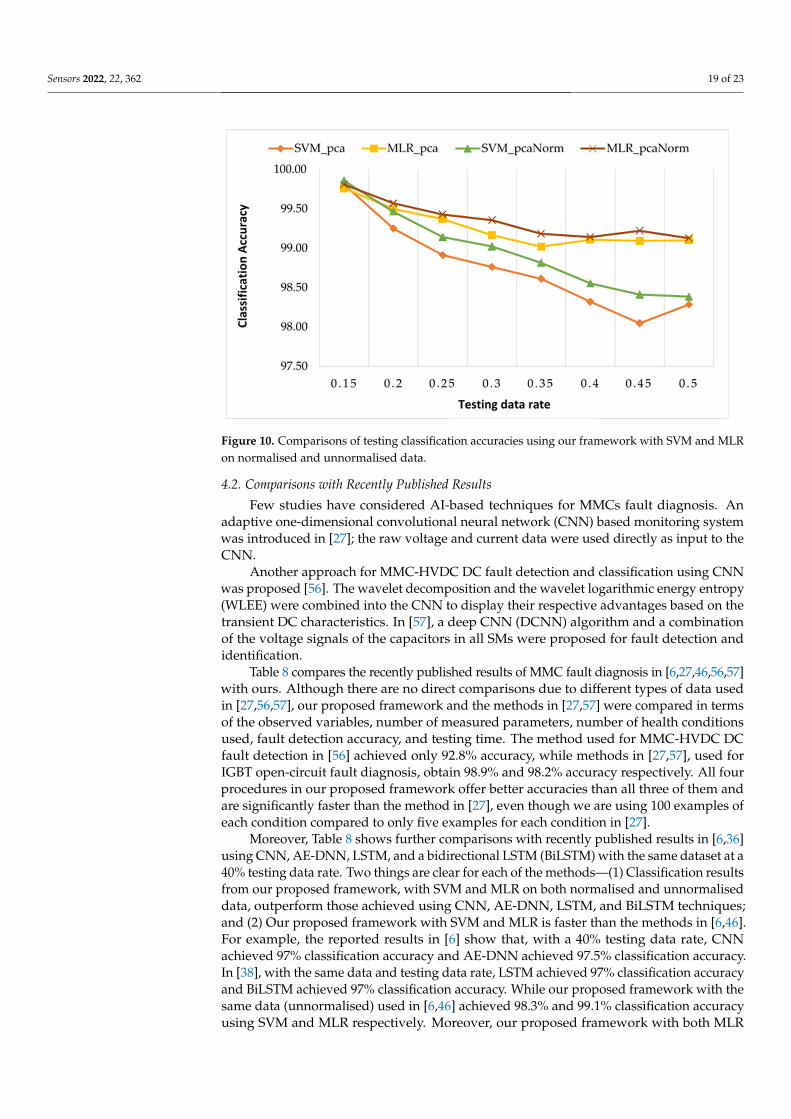
4.1. Comparisons of Testing Classifications

Figure 10 provides a comparison of testing classification results achieved using ourframework with SVM and MLR. From Figure 10, it is apparent that the classificationaccuracies of MMCs health condition using our framework with all four combinations arethe same at 15% of the testing rate. Additionally, in each of MLR and SVM, results withnormalised data are better than those with unnormalised data. For larger than 15% of thetesting rate, MLR results are better than SVM results on both normalised and unnormaliseddata. Additionally, MLR testing takes significantly less than a 10th of the time of SVM.

Sensors 2022, 22, 362 19 of 23Sensors 2022, 22, x FOR PEER REVIEW 20 of 24

Figure 10. Comparisons of testing classification accuracies using our framework with SVM and MLR on normalised and unnormalised data.

4.2. Comparisons with Recently Published Results Few studies have considered AI-based techniques for MMCs fault diagnosis. An

adaptive one-dimensional convolutional neural network (CNN) based monitoring system was introduced in [27]; the raw voltage and current data were used directly as input to the CNN.

Another approach for MMC-HVDC DC fault detection and classification using CNN was proposed [56]. The wavelet decomposition and the wavelet logarithmic energy en-tropy (WLEE) were combined into the CNN to display their respective advantages based on the transient DC characteristics. In [57], a deep CNN (DCNN) algorithm and a combi-nation of the voltage signals of the capacitors in all SMs were proposed for fault detection and identification.

Table 8 compares the recently published results of MMC fault diagnosis in [6,27,46,56,57] with ours. Although there are no direct comparisons due to different types of data used in [27,56,57], our proposed framework and the methods in [27,57] were com-pared in terms of the observed variables, number of measured parameters, number of health conditions used, fault detection accuracy, and testing time. The method used for MMC-HVDC DC fault detection in [56] achieved only 92.8% accuracy, while methods in [27,57], used for IGBT open-circuit fault diagnosis, obtain 98.9% and 98.2% accuracy re-spectively. All four procedures in our proposed framework offer better accuracies than all three of them and are significantly faster than the method in [27], even though we are using 100 examples of each condition compared to only five examples for each condition in [27].

Moreover, Table 8 shows further comparisons with recently published results in [6,36] using CNN, AE-DNN, LSTM, and a bidirectional LSTM (BiLSTM) with the same dataset at a 40% testing data rate. Two things are clear for each of the methods—(1) Clas-sification results from our proposed framework, with SVM and MLR on both normalised and unnormalised data, outperform those achieved using CNN, AE-DNN, LSTM, and BiLSTM techniques; and (2) Our proposed framework with SVM and MLR is faster than the methods in [6,46]. For example, the reported results in [6] show that, with a 40% testing data rate, CNN achieved 97% classification accuracy and AE-DNN achieved 97.5%

Figure 10. Comparisons of testing classification accuracies using our framework with SVM and MLRon normalised and unnormalised data.

4.2. Comparisons with Recently Published Results

Few studies have considered AI-based techniques for MMCs fault diagnosis. Anadaptive one-dimensional convolutional neural network (CNN) based monitoring systemwas introduced in [27]; the raw voltage and current data were used directly as input to theCNN.

Another approach for MMC-HVDC DC fault detection and classification using CNNwas proposed [56]. The wavelet decomposition and the wavelet logarithmic energy entropy(WLEE) were combined into the CNN to display their respective advantages based on thetransient DC characteristics. In [57], a deep CNN (DCNN) algorithm and a combinationof the voltage signals of the capacitors in all SMs were proposed for fault detection andidentification.

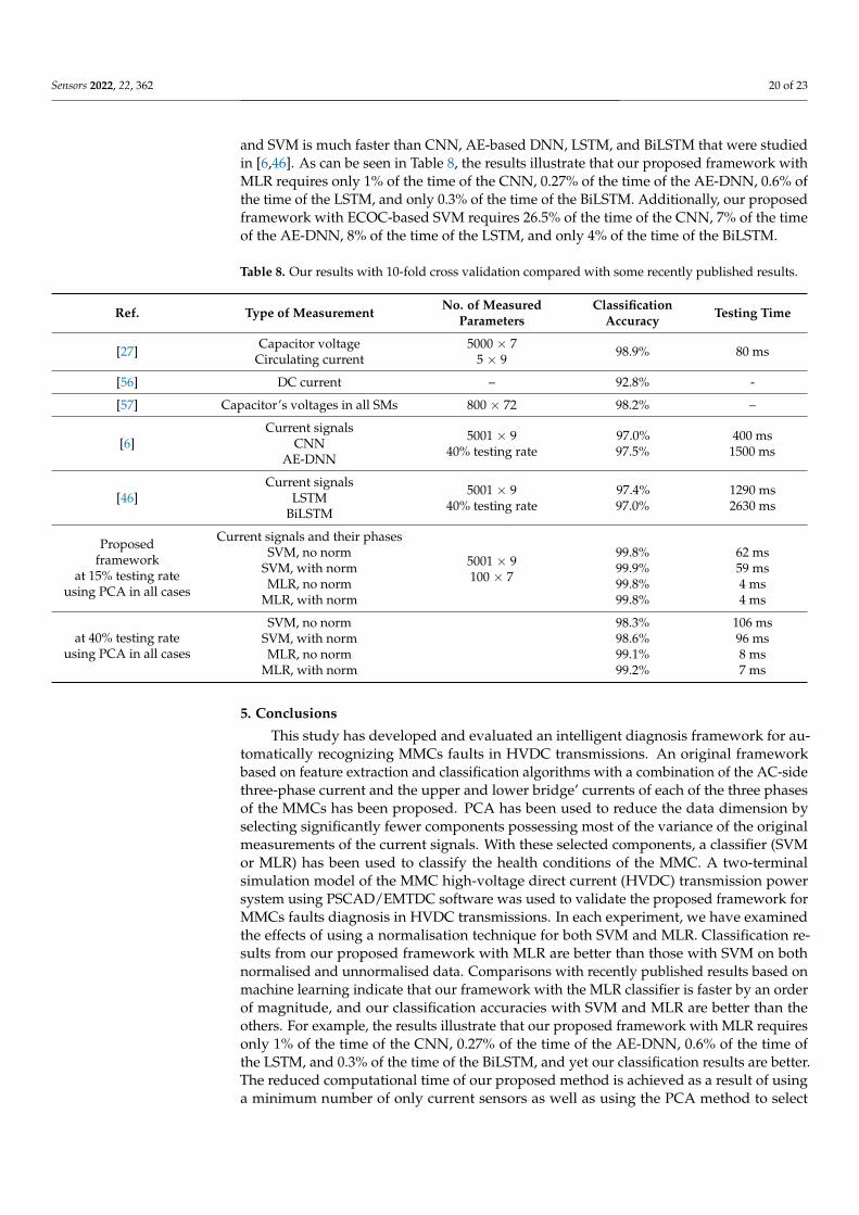
Table 8 compares the recently published results of MMC fault diagnosis in [6,27,46,56,57]with ours. Although there are no direct comparisons due to different types of data usedin [27,56,57], our proposed framework and the methods in [27,57] were compared in termsof the observed variables, number of measured parameters, number of health conditionsused, fault detection accuracy, and testing time. The method used for MMC-HVDC DCfault detection in [56] achieved only 92.8% accuracy, while methods in [27,57], used forIGBT open-circuit fault diagnosis, obtain 98.9% and 98.2% accuracy respectively. All fourprocedures in our proposed framework offer better accuracies than all three of them andare significantly faster than the method in [27], even though we are using 100 examples ofeach condition compared to only five examples for each condition in [27].

Moreover, Table 8 shows further comparisons with recently published results in [6,36]using CNN, AE-DNN, LSTM, and a bidirectional LSTM (BiLSTM) with the same dataset at a40% testing data rate. Two things are clear for each of the methods—(1) Classification resultsfrom our proposed framework, with SVM and MLR on both normalised and unnormaliseddata, outperform those achieved using CNN, AE-DNN, LSTM, and BiLSTM techniques;and (2) Our proposed framework with SVM and MLR is faster than the methods in [6,46].For example, the reported results in [6] show that, with a 40% testing data rate, CNNachieved 97% classification accuracy and AE-DNN achieved 97.5% classification accuracy.In [38], with the same data and testing data rate, LSTM achieved 97% classification accuracyand BiLSTM achieved 97% classification accuracy. While our proposed framework with thesame data (unnormalised) used in [6,46] achieved 98.3% and 99.1% classification accuracyusing SVM and MLR respectively. Moreover, our proposed framework with both MLR

Sensors 2022, 22, 362 20 of 23

and SVM is much faster than CNN, AE-based DNN, LSTM, and BiLSTM that were studiedin [6,46]. As can be seen in Table 8, the results illustrate that our proposed framework withMLR requires only 1% of the time of the CNN, 0.27% of the time of the AE-DNN, 0.6% ofthe time of the LSTM, and only 0.3% of the time of the BiLSTM. Additionally, our proposedframework with ECOC-based SVM requires 26.5% of the time of the CNN, 7% of the timeof the AE-DNN, 8% of the time of the LSTM, and only 4% of the time of the BiLSTM.

Table 8. Our results with 10-fold cross validation compared with some recently published results.

Ref. Type of Measurement No. of MeasuredParameters

ClassificationAccuracy Testing Time

[27] Capacitor voltageCirculating current

5000 × 75 × 9 98.9% 80 ms

[56] DC current – 92.8% -

[57] Capacitor’s voltages in all SMs 800 × 72 98.2% –

[6]Current signals

CNNAE-DNN

5001 × 940% testing rate

97.0%97.5%

400 ms1500 ms

[46]Current signals

LSTMBiLSTM

5001 × 940% testing rate

97.4%97.0%

1290 ms2630 ms

Proposedframework

at 15% testing rateusing PCA in all cases

Current signals and their phases

5001 × 9100 × 7

SVM, no norm 99.8% 62 msSVM, with norm 99.9% 59 msMLR, no norm 99.8% 4 ms

MLR, with norm 99.8% 4 ms

at 40% testing rateusing PCA in all cases

SVM, no norm 98.3% 106 msSVM, with norm 98.6% 96 msMLR, no norm 99.1% 8 ms

MLR, with norm 99.2% 7 ms

5. Conclusions

This study has developed and evaluated an intelligent diagnosis framework for au-tomatically recognizing MMCs faults in HVDC transmissions. An original frameworkbased on feature extraction and classification algorithms with a combination of the AC-sidethree-phase current and the upper and lower bridge’ currents of each of the three phasesof the MMCs has been proposed. PCA has been used to reduce the data dimension byselecting significantly fewer components possessing most of the variance of the originalmeasurements of the current signals. With these selected components, a classifier (SVMor MLR) has been used to classify the health conditions of the MMC. A two-terminalsimulation model of the MMC high-voltage direct current (HVDC) transmission powersystem using PSCAD/EMTDC software was used to validate the proposed framework forMMCs faults diagnosis in HVDC transmissions. In each experiment, we have examinedthe effects of using a normalisation technique for both SVM and MLR. Classification re-sults from our proposed framework with MLR are better than those with SVM on bothnormalised and unnormalised data. Comparisons with recently published results based onmachine learning indicate that our framework with the MLR classifier is faster by an orderof magnitude, and our classification accuracies with SVM and MLR are better than theothers. For example, the results illustrate that our proposed framework with MLR requiresonly 1% of the time of the CNN, 0.27% of the time of the AE-DNN, 0.6% of the time ofthe LSTM, and 0.3% of the time of the BiLSTM, and yet our classification results are better.The reduced computational time of our proposed method is achieved as a result of usinga minimum number of only current sensors as well as using the PCA method to select

Sensors 2022, 22, 362 21 of 23

fewer features to train the classification algorithm—i.e., SVM and MLRC algorithms—andto classify the MMC-HVDC’s health conditions using the trained classification models.

Author Contributions: H.O.A.A. and A.K.N. conceived and designed this paper. Y.Y. generated theraw data. M.D. and Q.W. gave the best suggestions about these experiments. H.O.A.A. analysed thedata. H.O.A.A. and A.K.N. wrote a draft of the manuscript. All authors contributed to discussingthe results in the manuscript. All authors have read and agreed to the published version of themanuscript.

Funding: This research was funded by the National Natural Science Foundation of China, grant no.51105291; by the Shaanxi Provincial Science and Technology Agency, nos. 2020GY124, 2019GY-125,and 2018JQ5127; and by the Key Laboratory Project of the Department of Education of ShaanxiProvince, nos. 19JS034 and 18JS045.

Institutional Review Board Statement: Not applicable.

Informed Consent Statement: Not applicable.

Data Availability Statement: The data presented in this study may be available on request from thefirst author, Hosameldin O. A. Ahmed. The data are not publicly available due to privacy reasons.

Acknowledgments: This work has been supported by Brunel University London (UK) and theNational Fund for Study Abroad (China). Yuexiao Yu and Qinghua Wang would like to thank BrunelUniversity London (UK) for hosting them during the development and execution of this research.

Conflicts of Interest: The authors declare no conflict of interest.

References1. Kouro, S.; Malinowski, M.; Gopakumar, K.; Pou, J.; Franquelo, L.G.; Wu, B.; Rodriguez, J.; Pérez, M.A.; Leon, J.I. Recent advances

and industrial applications of multilevel converters. IEEE Trans. Ind. Electron. 2010, 57, 2553–2580. [CrossRef]2. Saeedifard, M.; Iravani, R.; Pou, J. A space vector modulation strategy for a back–to back five-level HVDC converter system. IEEE

Trans. Ind. Electron. 2009, 56, 452–466. [CrossRef]3. Gnanarathna, U.N.; Gole, A.M.; Jayasinghe, R.P. Efficient modeling of modular Multi-level HVDC converters (MMC) on

electromagnetic transient simulation programs. IEEE Trans. Power Deliv. 2014, 26, 316–324. [CrossRef]4. Marquardt, R. Stromrichterschaltungen Mit Verteilten Energiespeichern. German Patent DE10103031A1, 24 January 2001.5. Sharifabadi, K.; Harnefors, L.; Nee, H.P.; Norrga, S.; Teodorescu, R. Design, Control, and Application of Modular Multilevel Converters

for HVDC Transmission Systems; John Wiley & Sons: Hoboken, NJ, USA, 2016. [CrossRef]6. Wang, Q.; Yu, Y.; Ahmed, H.O.; Darwish, M.; Nandi, A.K. Fault detection and classification in MMC-HVDC systems using

learning methods. Sensors 2020, 20, 4438. [CrossRef] [PubMed]7. Yang, S.; Bryant, A.; Mawby, P.; Xiang, D.; Ran, L.; Tavner, P. An industry-based survey of reliability in power electronic converters.

IEEE Trans. Ind. Appl. 2011, 47, 1441–1451. [CrossRef]8. Lu, B.; Sharma, S.K. A literature review of IGBT fault diagnostic and protection methods for power inverters. IEEE Trans. Ind.

Appl. 2009, 45, 1770–1777. [CrossRef]9. Ciappa, M. Selected failure mechanisms of modern power modules. Microelectron. Reliab. 2002, 42, 653–667. [CrossRef]10. Nuutinen, P.; Peltoniemi, P.; Silventoinen, P. Short-circuit protection in a converter-fed low-voltage distribution network. IEEE

Trans. Power Electron. 2012, 28, 1587–1597. [CrossRef]11. Abdallah, M.M.; Hamad, M.S.; Helal, A.A. Fault detection and isolation of MMC under submodule open circuit fault. In

Proceedings of the 2017 Nineteenth International Middle East Power Systems Conference (MEPCON), Cairo, Egypt, 19–21December 2017; pp. 1195–1200. [CrossRef]

12. Estima, J.O.; Cardoso, A.J.M. A new algorithm for real-time multiple open-circuit fault diagnosis in voltage-fed PWM motordrives by the reference current errors. IEEE Trans. Ind. Electron. 2012, 60, 3496–3505. [CrossRef]

13. Liu, H.; Ma, K.; Wang, C.; Blaabjerg, F. Fault diagnosis and fault-tolerant control of modular multi-level converter high-voltageDC system: A review. Electric Power Compon. Syst. 2016, 44, 16–1759. [CrossRef]

14. Liu, H.; Loh, P.C.; Blaabjerg, F. Review of fault diagnosis and fault-tolerant control for modular multilevel converter of HVDC.In Proceedings of the IECON 2013-39th Annual Conference of the IEEE Industrial Electronics Society, Vienna, Austria, 10–13November 2013; pp. 1242–1247. [CrossRef]

15. Sen, M.; Alaraj, M.; Park, J.D. Open circuit fault detection and localization in modular multilevel converter. In Proceedings of theNorth American Power Symposium (NAPS), Denver, CO, USA, 18–20 September 2016; pp. 1–6. [CrossRef]

16. Khomfoi, S.; Tolbert, L.M. Fault diagnosis and reconfiguration for multilevel inverter drive using AI-based techniques. IEEETrans. Ind. Electron. 2007, 54, 2954–2968. [CrossRef]

Sensors 2022, 22, 362 22 of 23

17. Song, W.; Huang, A.Q. Fault-tolerant design and control strategy for cascaded H-bridge multilevel converter-based STATCOM.IEEE Trans. Ind. Electron. 2009, 57, 2700–2708. [CrossRef]

18. Sedghi, S.; Dastfan, A.; Ahmadyfard, A. Fault detection of a seven level modular multilevel inverter via voltage histogram andneural network. In Proceedings of the IEEE 8th International Conference on Power Electronics-ECCE Asia, Jeju, Korea, 30 May–3June 2011; pp. 1005–1012. [CrossRef]

19. Jiang, W.; Wang, C.; Li, Y.P.; Wang, M. Fault detection and remedy of multilevel inverter based on BP neural network. InProceedings of the 2012 Asia-Pacific Power and Energy Engineering Conference, Shanghai, China, 27–29 March 2012; pp. 1–4.[CrossRef]

20. Lezana, P.; Aguilera, R.; Rodríguez, J. Fault detection on multicell converter based on output voltage frequency analysis. IEEETrans. Ind. Electron. 2009, 56, 2275–2283. [CrossRef]

21. Yazdani, A.; Sepahvand, H.; Crow, M.L.; Ferdowsi, M. Fault detection and mitigation in multilevel converter STATCOMs. IEEETrans. Ind. Electron. 2010, 58, 1307–1315. [CrossRef]

22. Wang, T.; Xu, H.; Han, J.; Elbouchikhi, E.; Benbouzid, M.E.H. Cascaded H-bridge multilevel inverter system fault diagnosis usinga PCA and multiclass relevance vector machine approach. IEEE Trans. Power Electron. 2015, 30, 7006–7018. [CrossRef]

23. Hu, X.; Zhang, J.; Xu, S.; Deng, F. Detection and location of open-circuit fault for modular multilevel converter. Int. J. Electr. PowerEnergy Syst. 2020, 115, 105425. [CrossRef]

24. Shao, S.; Wheeler, P.W.; Clare, J.C.; Watson, A.J. Fault detection for modular multilevel converters based on sliding mode observer.IEEE Trans. Power Electron. 2013, 28, 4867–4872. [CrossRef]

25. Shao, S.; Watson, A.J.; Clare, J.C.; Wheeler, P.W. Robustness analysis and experimental validation of a fault detection and isolationmethod for the modular multilevel converter. IEEE Trans. Power Electron. 2015, 31, 3794–3805. [CrossRef]

26. Pu, L.I.N.; ZHANG, Z.; ZHANG, Z.; Kang, L.; Wang, X. Open-circuit Fault Diagnosis for Modular Multilevel Converter UsingWavelet Neural Network. In Proceedings of the 2019 IEEE Innovative Smart Grid Technologies-Asia (ISGT Asia), Chengdu,China, 21–24 May 2019; pp. 250–255. [CrossRef]

27. Jiao, W.; Liu, Z.; Zhang, Y. Fault Diagnosis of Modular Multilevel Converter with FA-SVM Algorithm. In Proceedings of the 2019Chinese Control Conference (CCC), Guangzhou, China, 27–30 July 2019; pp. 5093–5098. [CrossRef]

28. Kiranyaz, S.; Gastli, A.; Ben-Brahim, L.; Al-Emadi, N.; Gabbouj, M. Real-time fault detection and identification for MMC using1-D convolutional neural networks. IEEE Trans. Ind. Electron. 2018, 66, 8760–8771. [CrossRef]

29. Li, C.; Liu, Z.; Zhang, Y.; Chai, L.; Xu, B. Diagnosis and location of the open-circuit fault in modular multilevel converters: Animproved machine learning method. Neurocomputing 2019, 28, 58–66. [CrossRef]

30. Chen, H.; Wang, J.; Liu, J.; Rehman, B.; Qian, F.; Liu, C. Validation Method for Simulation Model of Internet of Things-AidedPower System. IEEE Access 2019, 8, 1185–1192. [CrossRef]

31. Yang, Q.; Qin, J.; Saeedifard, M. Analysis, detection, and location of open-switch submodule failures in a modular multilevelconverter. IEEE Trans. Power Deliv. 2015, 31, 155–164. [CrossRef]

32. Huai, Q.; Liu, K.; Hooshyar, A.; Ding, H.; Chen, K.; Liang, Q. Single-ended line fault location method for multi-terminal HVDCsystem based on optimized variational mode decomposition. Electr. Power Syst. Res. 2021, 194, 107054. [CrossRef]

33. Han, Y.; Qi, W.; Ding, N.; Geng, Z. Short-time wavelet entropy integrating improved LSTM for fault diagnosis of modularmultilevel converter. IEEE Trans. Cybern. 2021, 1–9. [CrossRef] [PubMed]

34. Xing, W.; Yang, H.; Sheng, J.; Chang, X.; Li, W.; He, X. Open-circuit Fault Detection and Location in MMCs with MultivariateGaussian Distribution. In Proceedings of the 2020 4th IEEE International Conference on HVDC (HVDC), Xi’an, China, 6–9November 2020; pp. 555–559. [CrossRef]

35. Ye, X.; Lan, S.; Xiao, S.J.; Yuan, Y. Single Pole-to-Ground Fault Location Method for MMC-HVDC System Using WaveletDecomposition and DBN. IEEJ Trans. Electr. Electron. Eng. 2021, 16, 238–247. [CrossRef]

36. Shen, Y.; Wang, T.; Amirat, Y.; Chen, G. IGBT Open-Circuit Fault Diagnosis for MMC Submodules Based on Weighted-AmplitudePermutation Entropy and DS Evidence Fusion Theory. Machines 2021, 9, 317. [CrossRef]

37. Ke, L.; Zhang, Y.; Yang, B.; Luo, Z.; Liu, Z. Fault diagnosis with synchrosqueezing transform and optimized deep convolutionalneural network: An application in modular multilevel converters. Neurocomputing 2021, 21, 24–33. [CrossRef]

38. Guo, Q.; Zhang, X.; Li, J.; Li, G. Fault diagnosis of modular multilevel converter based on adaptive chirp mode decompositionand temporal convolutional network. Eng. Appl. Artif. Intell. 2022, 107, 104544. [CrossRef]

39. Reddy, G.A.; Shukla, A. Arm current sensor-less control of MMC for Circulating current suppression. In Proceedings of the 2019IEEE Energy Conversion Congress and Exposition (ECCE), Baltimore, MD, USA, 29 September–3 October 2019; pp. 6905–6910.[CrossRef]

40. Chen, X.; Liu, J.; Deng, Z.; Song, S.; Ouyang, S. IGBT Open-Circuit Fault Diagnosis for Modular Multilevel Converter WithReduced-Number of Voltage Sensor Measuring Technique. In Proceedings of the 2019 IEEE 10th International Symposium onPower Electronics for Distributed Generation Systems (PEDG), Xi’an, China, 3–6 June 2019; pp. 47–50. [CrossRef]

41. Xu, K.; Xie, S.; Yan, Y.; Zhang, Z.; Zhang, B.; Qian, Q. A fast fault diagnosis method for submodule failures in modular multilevelconverters. In Proceedings of the 2017 IEEE Energy Conversion Congress and Exposition (ECCE), Cincinnati, OH, USA, 1–5October 2017; pp. 1125–1130. [CrossRef]

42. Li, B.; Shi, S.; Wang, B.; Wang, G.; Wang, W.; Xu, D. Fault diagnosis and tolerant control of single IGBT open-circuit failure inmodular multilevel converters. IEEE Trans. Power Electron. 2015, 31, 3165–3176. [CrossRef]

Sensors 2022, 22, 362 23 of 23

43. Yang, S.; Tang, Y.; Wang, P. Seamless fault-tolerant operation of a modular multilevel converter with switch open-circuit faultdiagnosis in a distributed control architecture. IEEE Trans. Power Electron. 2018, 33, 7058–7070. [CrossRef]

44. Deng, F.; Chen, Z.; Khan, M.R.; Zhu, R. Fault detection and localization method for modular multilevel converters. IEEE Trans.Power Electron. 2014, 30, 2721–2732. [CrossRef]

45. Shao, S.; Wheeler, P.W.; Clare, J.C.; Watson, A.J. Open-circuit fault detection and isolation for modular multilevel converter basedon sliding mode observer. In Proceedings of the 15th European Conference on Power Electronics and Applications (EPE)-IEEE,Lille, France, 2–6 September 2013; pp. 1–9. [CrossRef]

46. Wang, Q.; Yu, Y.; Ahmed, H.O.; Darwish, M.; Nandi, A.K. Open-Circuit Fault Detection and Classification of Modular MultilevelConverters in High Voltage Direct Current Systems (MMC-HVDC) with Long Short-Term Memory (LSTM) Method. Sensors 2021,21, 4159. [CrossRef] [PubMed]

47. Anaya-Lara, O.; Acha, E. Modeling and analysis of custom power systems by PSCAD/EMTDC. IEEE Trans. Power Deliv. 2002, 17,266–272. [CrossRef]

48. Pearson, K. LIII: On lines and planes of closest fit to systems of points in space. Lond. Edinb. Dublin Philos. Mag. J. Sci. 1901, 2,559–572. [CrossRef]

49. Cortes, C.; Vapnik, V. Support-vector networks. Mach. Learn. 1995, 20, 273–297. [CrossRef]50. Gunn, S.R. Support vector machines for classification and regression. ISIS Tech. Rep. 1998, 14, 5–16.51. Mathworks.com. Fit Multiclass Models for Support Vector Machines or Other Classifiers—MATLAB Fitcecoc. 2017. Available

online: http://uk.mathworks.com/help/stats-/fitcecoc.html (accessed on 25 July 2021).52. Ahmed, H.; Nandi, A.K. Compressive sampling and feature ranking framework for bearing fault classification with vibration

signals. IEEE Access 2018, 6, 44731–44746. [CrossRef]53. Ahmed, H.O.; Nandi, A.K. Three-stage hybrid fault diagnosis for rolling bearings with compressively sampled data and subspace

learning techniques. IEEE Trans. Ind. Electron. 2018, 66, 5516–5524. [CrossRef]54. Ahmed, H.O.A.; Wong, M.L.D.; Nandi, A.K. Intelligent condition monitoring method for bearing faults from highly compressed

measurements using sparse over-complete features. Mech. Syst. Signal Processing 2018, 99, 459–477. [CrossRef]55. Ahmed, H.O.; Nandi, A.K. Condition Monitoring with Vibration Signals: Compressive Sampling and Learning Algorithms for Rotating

Machines; John Wiley & Sons: Hoboken, NJ, USA, 2020.56. Wang, J.; Zheng, X.; Tai, N. DC Fault Detection and Classification Approach of MMC-HVDC Based on Convolutional Neural

Network. In Proceedings of the 2018 2nd IEEE Conference on Energy Internet and Energy System Integration (EI2), Beijing,China, 20–22 October 2018; pp. 1–6. [CrossRef]

57. Qu, X.; Duan, B.; Yin, Q.; Shen, M.; Yan, Y. Deep Convolution Neural Network Based Fault Detection and Identification forModular Multilevel Converters. In Proceedings of the 2018 IEEE Power & Energy Society General Meeting (PESGM), Portland,OR, USA, 5–10 August 2018; pp. 1–5. [CrossRef]