Spatial distribution maps for benthic communities

Spatial distribution maps forbenthic communities

A study of common mussels (Mytilus edulis), neptune grass(Posidonia oceanica), and Cymodocea nodosa based on

hydroacoustic measurements

Per Settergren Sørensen

Lyngby 1999Department of Mathematical Modelling

Technical University of Denmark

Ph.d. Thesis

Name Per Settergren Sørensen, M.Sc.Eng. (CE87)

Ph.d number 96-0169-221

Ph.d programme Mathematics

Institute Department of Mathematical Modelling (IMM)

Start date November 1st, 1996

End date July 31st, 1999

Supervisor Professor Knut Conradsen, IMM

Co-supervisor Associate Professor Bjarne Kjær Ersbøll, IMM

Copyright 1999by Per Settergren Sørensen

Preface

This thesis has been prepared at the Section for Image Analysis, Department of MathematicalModelling, Technical University of Denmark, in partial fulfillment of the requirements foracquiring the Ph.D. degree in engineering.

The general framework of this thesis is statistics, in particular geostatistics and statistical imageanalysis, and the application domain is hydroacoustic marine biology. Reading this thesisrequires a basic knowledge of multivariate statistics.

The object of the thesis is the preparation of maps depicting spatial distribution of mussels andseagrasses on the sea floor based on hydroacoustic measurements. The report gives a treatmentof some of the statistical challenges arising from the special data types and sampling designspresented by hydroacoustic measurements, in particular echo sounder measurements. The mainresult is that it is feasible to use hydroacoustic measurements to prepare spatial distributionmaps at large scales with a relatively high resolution.

The application of a large and unique collection of hydroacoustic datasets has been a major partof the work, from the planning of observational designs to the data analysis leading to spatialdistribution maps. Therefore, the elaboration of a well-founded alignment of methods ofgeostatistics, image analysis and multivariate statistics in an appropriate data processing schemehas been a main objective. The use of mathematics and statistics in this thesis can be conceivedof as a tour around the image modelling marketplace, yet it is my hope that the presentation iscoherent and adequate. Hopefully, the results can inspire further developments of dataprocessing methodology for hydroacoustic measurements in regard to sea floor mapping.

Lyngby, November 5th, 1999

Per Settergren Sørensen

ii

Acknowledgements

I am indebted to my supervisor Professor Knut Conradsen, Head of the Section for ImageAnalysis, for encouraging and guiding many steps throughout this work and for letting medepend on his knowledge of mathematics and statistics. I thank my co-supervisor AssociateProfessor Bjarne Kjær Ersbøll and Associate Research Professor Allan Aasbjerg Nielsen fortheir prompt help and many valuable suggestions; during the last 3 years of close collaborationAllan contributed a frank and direct atmosphere that has been stimulating and fruitful.Furthermore, I acknowledge the prompt services by Secretary Helle Welling and the advice onMCMC from Assoc. Professor Jens Michael Carstensen, and the contributions from Ass.Research Professor Nette Schultz and Assoc. Research Professor Anette Ersbøll, all from IMM.

At VKI, my work place, I would like to acknowledge the enthusiasm and energy provided bymy marine biologist colleague and close collaborator M.Sc. Kristian Madsen. Words ofgratitude go to the head of my department, Arne Hurup Nielsen, and to the director of ourdivision, Kurt Jensen, for their professional and financial support, and to my colleagues for helpwith the manuscript and with debugging of my Delphi 3 code. I thank M.Sc. Kasper Hornbækfor many valuable comments made during the finalisation of the manuscript. Special thoughtsof appreciation go to my former colleague Professor Jes la Cour Jansen, Department of Buildingand Environmental Technology, Lund University, Sweden, for showing me the entrance to thescientific world many years ago and helping me through the gates.

I acknowledge the geometric approach to statistical image analysis taught me by AssistantResearch Professor Mads Nielsen, 3D-Lab, School of Dentistry, University of Copenhagen,during the course in the spring 1998, as well as the energetic work conducted by my fellowstudent cand.silv. Mads Jeppe Tarp-Johansen from DINA, KVL.

I am grateful to Professor Peter Guttorp, Department of Statistics and director of NRCSE at theUniversity of Washington, Seattle, USA, for giving me the opportunity to visit the NationalResearch Centre for Statistics and the Environment (NRCSE) in September and October 1998.Thanks goes to NRCSE fellows Joel Reynolds and David Caccia for their comments andsuggestions and to Professor Paul Sampson and Dean Billheimer for valuable discussions, andto Erik Christiansson and Gerry Goedde for their support during my stay at Bagley Hall.

Thanks to the kind providers of data, Jorge Rey at Estudios Geologicos Marinos (ESGEMAR),Málaga, Patricia Siljeström at IRNASE/CSIC, Sevilla, Ola Oskarsson at MMT, Göteborg, andto Klas Vikgren for providing the video strip-charts. I thank all participants in the BioSonarproject for their contributions, which have been inspiring and amending some of the steps takenin this thesis; I am particularly grateful for many hours of good company and inspiringdiscussions with Kristian, Allan and Knut. The support and funding from the Commission ofthe European Union under contract no. MAS3-CT95-0026 with the MAST office of DG XII ishighly appreciated. The funding received from Øresundskonsortiet is acknowledged.

Finally, I would like to thank my friends and family, Janne, Amanda and Valdemar (arriving inthe middle of the study), as well as Katrine and Charlotte for being there and for their supportand patience in times of high work load, in particular in the phase of finalising the manuscript.

It goes without saying that without all the fine people mentioned and the funding received Iwould not have been able to carry out this work.

iii

Abstract

The application of hydroacoustic measurements for preparation of spatial distribution maps ofbenthic communities is reported. For the present study common mussels (Mytilus edulis),neptune grass (Posidonia oceanica) and Cymodocea nodosa, serving as canonical species ofmany European marine ecosystems, were selected. These species are supposed to be goodindicators of marine ecosystem health. The hydroacoustic measurements comprisepreprocessed echo sounder recordings and side-scan sonar data forming a large and uniquecollection of datasets based on 4 field campaigns in Øresund and the Mediterranean. Acombination of geostatistical methods for spatial interpolation of the echo sounder observationsand a set of classification rules, based on discriminant analysis of the feature space of theobservations, is found to yield reliable distribution maps when compared to groundtruth data.The data-driven methodology developed is shown to be adaptive to instationarities in the echosounder observations and is recommended as a substantial improvement of existing methods ofsea floor mapping based on echo sounder data.

Elaborations of the developed methodology are studied, comprising the use of geostatisticalsimulation, Markov random fields and Boolean models. Geostatistical simulation provides ameans of assessing the variability of random field functionals such as the estimated distributionarea of a benthic species. The Markov random field allows the spatial distribution of thebenthic communities to be modelled as a less smooth or regular phenomena than assumed whenusing geostatistical models. The use of Markov random fields in a Markov chain Monte Carlosimulation framework enables an alternative means of assessing variability of image functionalsthat is based on a sound theoretical basis. The estimates of variability obtained for estimateddistribution areas with the two approaches compare satisfactorily. The Boolean models aresuggested as a point of departure for embedding models of spatial patterns on the minor scalesof observations to be used in up-scaling approaches to enhance the quality of the distributionmaps and to be combined with biogeochemical models describing spatiotemporal populationdynamics.

Finally, the use of side-scan sonar data is illustrated in a data fusion exercise combining side-scan sonar data with the results based on echo sounder measurements. The feasible use of side-scan sonar for mapping of benthic communities remains an open task to be studied in the future.

The data processing methodology developed is a contribution to the emerging field ofhydroacoustic marine biology. The method of penalised maximum pseudo-likelihood forestimation of the Ising model under a huge amount of missing pixel data is a contribution tostatistical image analysis. Furthermore, the estimation method developed for non-stationaryBoolean models that combines scale-space kernel smoothing with the so-called method-of-moments applied to stationary Boolean models is a contribution to stochastic geometry.

iv

Sammenfatning

Et studie af anvendelsen af hydroakustiske målinger til kortlægning af benthiske samfundsudbredelse beskrives. Blåmuslinger (Mytilus edulis), neptungræs (Posidonia oceanica) ogCymodocea nodosa blev udvalgt, da disse arter er af grundlæggende betydning for mangemarine europæiske økosystemer. Disse arter antages således at være gode indikatorer for demarine økosystemers sundhed. De hydroakustiske målinger omfatter præprocesseredeekkolodsmålinger og side-scan sonar målinger, som udgør en enestående samling af datasætindsamlet under 4 feltkampagner i Øresund og Middelhavet. Studierne viser, at en kombinationaf geostatistiske metoder til spatiel interpolation af ekkolodsmålinger med klassifikationsregler,som er baseret på diskriminantanalyser af målingernes faserum, resulterer i udbredelseskort,hvis pålidelighed kan verificeres vha. groundtruth data. Det bliver eftervist, at den udviklededata-drevne metodologi er adaptiv mht. manglende stationaritet mellem ekkolodsmålinger, ogden anbefales således som en væsentlig forbedring af eksisterende metoder til kortlægning afhavbunden vha. ekkolodsmålinger.

Forskellige elaboreringer af den udviklede metodologi er efterfølgende undersøgt, omfattendebrug af geostatistisk simulation, Markov felter og Boolean models. Geostatistisk simulation eret redskab til estimering af variabilitet for funktionaler af stokastiske felter såsom estimeredeudbredelsesarealer for benthiske samfund. Ved brug af Markov felter er det muligt at modellerebenthiske samfunds udbredelse som teksturer, dvs. spatielle stokastiske felter med mindreglathed og regularitet end forudsat, når geostatistiske metoder anvendes. Anvendelse af Markovfelt modeller til simulation inden for et såkaldt Markov chain Monte Carlo paradigme er enalternativ metode til estimation af variabilitet for udbredelsesarealer, som har en attraktivteoretisk fundering. Variansestimater beregnet med de to simulationsmetoder udviser godoverensstemmelse. Boolean models foreslås som et middel til at indlejre viden om spatiellemønstre, som er karakteristiske for hvert enkelt benthisk samfund på de mindre skalaer, medsigte på dels at forbedre udbredelseskortenes opløsning og præcision, dels at kunne kombinereudbredelseskortene med biogeokemiske modeller til beskrivelse af spatiotemporalpopulationsdynamik.

Anvendelse af side-scan sonar data illustreres i en datafusionsøvelse, hvori side-scan sonar datakombineres med resultater baseret på ekkolodsmålinger. Gode anvendelsesmetoder for side-scan sonar data med henblik på at fremstille udbredelseskort for bentiske samfund er et åbentproblem, som vil blive studeret fremover.

Den udviklede metodologi for processering af hydroakustiske data er et bidrag til det for tidenfremvoksende felt hydroakustisk marinbiologi. Den udviklede estimationsmetode for Isingmodellens parametre under store mængder manglende pixelværdier i et billede, som er baseretpå penalised maximum pseudo-likelihood, er et bidrag til statistisk billedanalyse. Den for ikke-stationære Boolean models udviklede estimationsmetode, som kombinerer udglatninger i etskalarum med den såkaldte moment-metode for stationære Boolean models, er et bidrag tilmetoder inden for stokastisk geometri.

v

Table of Contents

Preface.............................................................................................................................................................................i

Acknowledgements .....................................................................................................................................................ii

Abstract....................................................................................................................................................................... iii

Sammenfatning........................................................................................................................................................... iv

1 INTRODUCTION.....................................................................................................1

1.1 Background and objectives .......................................................................................................................11.1.1 Background ........................................................................................................................................... 11.1.2 Objectives .............................................................................................................................................. 2

1.2 Contexts ..........................................................................................................................................................31.2.1 Interdisciplinary scientific context ..................................................................................................... 31.2.2 Mathematical-statistical context ......................................................................................................... 51.2.3 The context of marine biology ........................................................................................................... 61.2.4 Scope and field of applications.......................................................................................................... 71.2.5 Scale of spatial distribution maps...................................................................................................... 71.2.6 Delimitation........................................................................................................................................... 7

1.3 The target species.........................................................................................................................................81.3.1 Common mussels ................................................................................................................................. 81.3.2 Neptune grass (Posidonia oceanica)................................................................................................. 9

1.4 Applied software and previous publications.........................................................................................9

1.5 Outline of the thesis...................................................................................................................................10

2 DATA MATERIAL................................................................................................ 11

2.1 Field campaigns and data acquisition...................................................................................................112.1.1 Design of field campaigns ................................................................................................................ 122.1.2 Execution of the field campaigns in 1996...................................................................................... 162.1.3 Execution of the field campaigns in 1997...................................................................................... 16

2.2 Available and selected data......................................................................................................................162.2.1 Echo sounder data recorded in Øresund......................................................................................... 162.2.2 Echo sounder data recorded at Cartagena ...................................................................................... 172.2.3 Side-scan sonar data .......................................................................................................................... 17

2.3 Groundtruth data.......................................................................................................................................17

3 GEOSTATISTICAL DISTRIBUTION MAPS FOR MUSSELS..................... 19

3.1 Semivariograms and kriging ..................................................................................................................193.1.1 Introduction to the theory of geostatistics...................................................................................... 193.1.2 The practice of semivariograms and kriging.................................................................................. 273.1.3 Semivariograms for the bottom type areas .................................................................................... 283.1.4 Semivariograms for the test areas ................................................................................................... 35

vi

3.2 Classification of feature spaces...............................................................................................................393.2.1 Classification and discriminant analysis ........................................................................................ 393.1.2 Estimation of classification regions ................................................................................................ 403.1.3 Classification of the test areas.......................................................................................................... 453.1.4 Interpretations ..................................................................................................................................... 47

3.3 Preparation of distribution maps and estimates of distribution areas ........................................483.3.1 Validation maps for the bottom type areas .................................................................................... 483.3.2 Distribution maps for test area 1, Drogden South ........................................................................ 513.3.3 Distribution maps for test area 2, Flinterenden NW..................................................................... 58

3.4 Change detection in mussel distribution maps ...................................................................................63

3.5 Groundtruthing and verification ...........................................................................................................69

3.6 Summary and discussion..........................................................................................................................76

4 SPATIAL DISTRIBUTION MAPS FOR SEAGRASSES............................... 79

4.1 Descriptive statistics and variograms ...................................................................................................794.1.1 The datasets from the bottom type areas at Cabo de Palos ......................................................... 794.1.2 The dataset for the test area at Cabo de Palos ............................................................................... 824.1.3 Semivariograms .................................................................................................................................. 84

4.2 Feature space classification .....................................................................................................................85

4.3 Spatial distribution maps for Cymodocea nodosa .............................................................................87

4.4 Discussion.....................................................................................................................................................89

5 GEOSTATISTICAL SIMULATION OF MUSSEL DISTRIBUTION MAPS. 91

5.1 Introduction to geostatistical simulation..............................................................................................915.1.1 Basic theory of conditional geostatistical simulation................................................................... 925.1.2 The practice of conditional geostatistical simulation ................................................................... 93

5.2 Simulation-based assessment of variability.........................................................................................945.2.1 The steps of the simulation ............................................................................................................... 955.2.2 Results and subsequent analyses ..................................................................................................... 98

5.3 Discussion.................................................................................................................................................. 101

6 A MARKOV RANDOM FIELD APPROACH TO DISTRIBUTION MAPS OFMUSSELS ..................................................................................................................105

6.1 Introduction.............................................................................................................................................. 1056.1.1 Markov random fields......................................................................................................................1066.1.2 Markov chain Monte Carlo .............................................................................................................107

6.2 The Ising model........................................................................................................................................ 1086.2.1 Basic properties of the Ising model...............................................................................................1086.2.2 Simulation of the Ising model.........................................................................................................1126.2.3 Maximum likelihood estimation for the Ising model.................................................................113

6.3 Ising model estimation for images with missing data.................................................................... 1146.3.1 Maximum pseudo-likelihood for images containing missing data..........................................1156.3.2 Penalised maximum pseudo-likelihood........................................................................................119

vii

6.3.3 MCMC approximated ML estimation...........................................................................................125

6.4 Estimation and simulation of an Ising model for the study area............................................... 1296.4.1 Dataset for the core part of test area 1, 1997................................................................................1296.4.2 PMPL estimation for the Ising model...........................................................................................1306.4.3 Ising model simulations of mussel distribution maps................................................................131

6.5 Discussion.................................................................................................................................................. 132

7 SIDE-SCAN SONAR AND DATA FUSION...................................................135

7.1 Side-scan sonar data............................................................................................................................... 1357.1.1 Preprocessing and geocoding of Isis side-scan sonar data........................................................1367.1.2 Classification of Isis side-scan sonar images...............................................................................136

7.2 Data fusion studies .................................................................................................................................. 138

7.3 Discussion.................................................................................................................................................. 143

8 MODELS OF SPATIAL PATTERNS..............................................................145

8.1 Introduction.............................................................................................................................................. 1458.1.1 Mathematical morphology..............................................................................................................1458.1.2 Scale-space theory............................................................................................................................1478.1.3 Boolean models .................................................................................................................................1478.1.4 Other frameworks for modelling of spatial patterns ..................................................................148

8.2 Models of spatial patterns for mussels .............................................................................................. 1498.2.1 Basic formulation of a spatial pattern model for mussels .........................................................149

8.3 Estimation of non-stationary Boolean models ................................................................................ 1518.3.1 Introduction.......................................................................................................................................1518.3.2 Basic theory .......................................................................................................................................1518.3.3 Illustration of the estimation method for Posidonia oceanica .................................................152

9 SUMMARY AND CONCLUSIONS .................................................................157

9.1 Conclusions ............................................................................................................................................... 157

9.2 Outlook and perspectives ...................................................................................................................... 158

10 REFERENCES ...................................................................................................159

Appendix A: Preprocessing of echo sounder data from Øresund.Appendix B: Exploratory spatial data analysis of echo sounder data from Øresund.Appendix C: The preprocessing and geocoding of Isis side-scan sonar dataAppendix D: Software developedAppendix E: Relevant websites

1

1 Introduction

This ph.d. thesis investigates the use of various statistical image analysis methods for mappingof benthic communities, and suggests ways of combining data and models at different spatialscales into coherent maps of their spatial distribution. The present chapter gives a shortintroduction to the background and objectives of the studies, and outlines their scientific andmethodological contexts. Furthermore, potential applications are discussed shortly, and a briefintroduction to the targeted species is given.

1.1 Background and objectivesThe studies reported here aim at the production of reliable, large-scale, high resolutiondistribution maps for designated benthic communities. The results of the present studies viewedin common with the results of the BioSonar project (MAS3-CT95-0026, 1997; 1998; 1999)yield one of the first tenable bids for a data processing method that complies with these threeambitious objectives, in this author's opinion. The present ph.d. thesis is aimed at the applicationof a specific spatial data type for particular purposes rather than aiming at a study of a particularmathematical method; hence, the use, description and development of mathematics will bedetailed primarily in cases where it is found necessary or desirable. The specific property of thespatial data type under consideration is that it has a particular net-shaped structure of irregulardata locations, i.e. what is usually referred to as irregularly spaced data in geostatistics.

1.1.1 BackgroundThe biological material on the sea floor or partly immersed in it is called benthos or benthicmaterial (benthic = at the sea bottom). Benthic habitats are usually divided into a range oftypes, like it is done in terrestrial biogeography, described by so-called benthic communitiescharacterised by certain species being vital for the structures of benthic ecosystems. Benthiccommunities constitute the general object of the measurements and methods described here, asopposed to pelagic material (pelagic = in the water phase, above ground), i.e. fish and otherswimming organisms. In the world's oceans the benthic biomass at depths greater than 3000 mis probably less than 1 gm-2 wet weight, at depths between 200 m and 3000 m the world averageis about 20 gm-2, and for waters shallower than 200 m the average is about 200 gm-2; it has beencalculated that more than 80% of the marine benthic biomass of the world lives on thecontinental shelves at depths of 0 - 200 m (Barnes & Mann, 1991). The biological production inthese areas is one of the main drivers of global ecological cycles, and very important forhumankind too. With the rise of environmental awareness focus on the sustainability andbiodiversity of these coastal marine environments is increasing in many public and politicalcontexts.

Thus, monitoring of marine ecosystem health is becoming increasingly important, and newmethods must be explored to ensure the sufficient efficacy of environmental surveillance andcorresponding mapping of spatial distributions of target species and ecosystems. One group ofsurvey methods selects so-called indicator species, that is species canonical to wholeecosystems, and tries to evaluate the ecosystem health by assessing the state of the indicator

2

species. In the BioSonar project common mussels (Mytilus edulis) and neptune grass (Posidoniaoceanica) were selected as indicator species. During the project data were also collected for thespecies Cymodocea nodosa in the Mediterranean and eelgrass (Zostera marina) in Øresund,creating additional valuable datasets.

Usual marine biological methods for benthic investigations deal with in situ sampling of the seabottom, qualitative reports of diver's findings and occasionally still photos or subsea videosrecorded at the sea floor. The BioSonar project explored the opportunities of applyinghydroacoustic measurements and sonar recordings for benthic surveys, which was expected tobe a promising venture. The BioSonar project concerned how to produce reliable and precisedistribution maps for benthic communities at optimised costs, applying as many automatedprocesses as possible. One of the major challenges of the approach was that there were severalchains in the process needing refurbishment and elaboration in order to produce the resultingdistribution maps. The list of overall goals of the project included:

♦ Quantitative detection (ability to detect benthic communities, and the ability to characterisetheir density with satisfactory precision)

♦ Reliability (reproducible or traceable, objective methods)♦ Automation (computerisation of all possible work processes)♦ Change detection (methods for monitoring changes in benthic communities).

Therefore, the goal was to measure precision by quantitative methods, e.g. by use of so-calledresubstitution rates for classified images, and the processes should be automated as far aspossible. In this context automation means at least computerised as regards the overallprocessing from the gathering of raw data to the preparation of the distribution maps to beinserted in GIS systems. Some of these processes would possibly require subjective decisionsto be carried out during the use of computer programs, and might therefore not be totallyobjective or independent of the operator.

The present ph.d. thesis was prepared as a part of the work on the BioSonar project, and muchof the work was therefore largely overlapping with it. Hence, the overall goals of the of theBioSonar project apply here also, with the qualification that the present thesis is a study of asubset of the data material and the data types collected in the BioSonar project. A specificdescription of the BioSonar data material and the subset of the data material selected for thepresent ph.d. study is given in chapter 2.

1.1.2 ObjectivesThe objectives of the studies can be outlined as follows:

♦ To determine the feasibility and applicability of hydroacoustic measurements in the form ofecho sounder recordings and side-scan sonar images for preparation of distribution maps ofbenthic communities.

♦ To develop statistically sound data processing methods for preparation of distribution mapsbased on hydroacoustic measurements.

♦ To develop statistical methods for assessment of the uncertainty of distribution maps, inparticular of derived coverage area estimates.

♦ To suggest and estimate stochastic models of the spatial patterns of the selected benthiccommunities.

Stated in a more pictorial way the objectives are to develop the infrastructure and the black boxcontents of the general data flow diagram depicted in Figure 1.1.

3

Figure 1.1 An outline of the data flow involved in the preparation of spatial distribution mapsbased on hydroacoustic measurements.

1.2 ContextsThis section introduces various points of departure for describing the rationale and context ofthe present study. The contexts sketched in the following comprise an interdisciplinary scientificcontext, a mathematical context, a marine biological context and an application context, and alist of topics not included is given too.

1.2.1 Interdisciplinary scientific contextTo produce spatial distribution maps various disciplines must be brought together. The scientificand methodological fields can be divided into those contributing to the input, i.e. planning ofobservational designs and collection and acquisition of measurements, to the output, i.e. theproduction of (end user) spatial distribution maps, and to the intermediate processing linking theoutput to the input, cf. Figure 1.2.

In the input section remote sensing, marine biology and geostatistics applies to the design of thefield campaigns in tasks such as pointing out interesting survey areas and planning sailingtransect layouts. Backscatter theory and signal analysis applies to the hydroacousticsconsiderations of selecting the right instrumentation operating at the right frequencies, etc. andto the collection and preprocessing of electronic sensor signals. Finally, knowledge ofunderwater video (and photo) is a necessary component in the planning and execution ofgroundtruth data collection.

4

Input Processing / function Output

Marine biology

Remote sensing

Hydroacoustics,Backscatter theory &

Signal analysis

Geostatistics

UW video

Multivariate statistics

Spatial statistics, i.e. Geostatistics& Markov random fields

Stochastic geometry andmathematical morphology

Biogeochemical modelling

Backscatter theory

Cartography

Marine biology

GIS(Geographical

information systems)

Figure 1.2 Some of the disciplines involved in the preparation of spatial distribution maps onthe basis of hydroacoustic measurements. The list of fields given here is not intended to beexhaustive.

In the output section, the production of thematic maps belongs naturally under the field ofcartography, and GIS is included in the list to underline the electronic and digital nature of themaps produced. Marine biology enters as a verification means comparing output to groundtruthdata.

A selection of mathematically based data processing disciplines links input and output. Firstand foremost the use of spatial statistics and statistical image analysis, including geostatisticsand Markov random fields, is emphasized; in some cases it is advantageous to supplement andelaborate these methods by means of stochastic geometry and mathematical morphology. Toprovide links to the worldview of biologists and their lines of study a promising path for thefuture would be to integrate these stochastic models with population dynamics models, the latteroften having a principal deterministic content. This would allow the description of growthrates, seasonal behaviour patterns, etc. to enter the modelling; the term biogeochemicalmodelling in Figure 1.2 is hinting at this. In a more advanced setting, backscatter theory mightbe applied directly in the data processing when (or if) the measurement techniques reach a levelwhere various species can be differentiated and detected by the hydroacoustic backscattersignatures.

All these jigsaw puzzles can be put into one hat constituting a field that could be labeledhydroacoustic marine biology. The end product is a thematic map, that is a map wheresubregions have been coloured to indicate properties of interest, like e.g. nations depicted in anatlas; formally, every pixel of a thematic map has been assigned a value from a set of stipulatedthematic classes. Thus, a thematic map can be viewed as the product of a topographic map, i.e.a simple map of some measurement variables, and an interpretation of the measurements givenby e.g. a set of classification rules.

A few of the fields mentioned above are singled out for further introduction below.

5

1.2.2 Mathematical-statistical contextA basic dichotomy of mathematical statistics is that of separating signal from noise implicitlydefining most statistical models by the following canonical expression:

Y = µ + e (1.1)

where Y is a measurement, µ is the deterministic component of the measurement, and e is therandom component of the measurement. This dichotomy of a dual (deterministic, random)component is known under various names as e.g. (level, variability), (location, dispersion),(explained, unexplained), and (signal, noise), pertaining more or less to properties of the dualcomponents. These labels are not globally applicable, e.g. explainable components are notnecessarily deterministic, levels and locations can be rather fluctuating, noise might be quiteexplainable, etc. Hence, Tukey (1977) used the terms smooth and rough to give the notion ofthis dichotomy in a generic sense. One point of (1.1) is that the delimitation of the explainedcomponent µ and the random component e is defined subjectively by the person formulating themodel, probably guided by a formulation of the hypothesis to be investigated.

Here, the generic model (1.1) is applied over a 2-dimensional (2D) space, and hence it iswritten:

Z(s) = µ(s) + e(s) (1.2)

extending the random variable Y to the random field Z(s) defined on the underlying 2D space(the index set) containing the point s = (x,y)'. The expression (1.2) indicates that the spatialmeasurements are made up of a smooth spatial component µ(s) and a random (rough)component e(s).

Another basic observation to make from a statistical point of view is that the datasets studiedhere represent observational designs, i.e. they are measurements of a state of nature that is notcontrollable (yet...) by humankind as opposed to experimental designs aimed at studying effectsof varying a range of interesting, controllable factors. Observational designs have their ownbody of design and inference theory, and one of the original introductions to the subject can befound in Cochran (1983).

The random field Z(s) is normally studied by means of geostatistics if the index set isconsidered to be continuous and by means of theory and methods for random fields withdiscrete support if the index set is a discretised grid. For simplicity, treatment of the latter willbe restricted to Markov random fields.

Geostatistics emerged in the early 1970s and '80s as a hybrid discipline of mining engineering,geology, mathematics, and statistics, primarily elaborated and promoted by G. Matheron at theEcole des Mines in Paris. Its strength over more classical approaches to ore-reserve estimationlies in the inherent accounting for both large-scale and small-scale spatial variability, whereearlier methods like trend-surface methods accounted for large-scale variability only. Much ofgeostatistics terminology stems from its history of emergence, e.g. the class of optimal linearspatial prediction methods is called kriging owing to one of the originators D.G. Krige.Introductions to geostatistics can be found in Journel & Huijbregts (1978) and Isaaks &Srivastava (1989), and to spatial statistics in general in Cressie (1991). Some enlighteningremarks on the simultaneous development of computational power and geostatistics can befound in Myers (1999). In the present report, a more detailed introduction to geostatistics isgiven in section 3.2.1, and an introduction to geostatistical simulation is given in section 3.5.1.

6

Markov random fields theory is a basic modelling framework for statistical image analysiswhere images are conceived of as data organised in lattices (the technical term) and representedas pixels. Markov random fields describe small-scale variability by correlation between closelylocated pixels and provide good means for describing textures of images. Introductions toMarkov random fields are given in e.g. Cressie (1991), Carstensen (1992) and Guttorp (1995).

Together, the use of geostatistics and Markov random fields forms the backbone of spatialstatistics. A more eloquent definition of spatial statistics is given by Charlie Geyer: "Spatialstatistics, narrowly defined, is the study of stochastic processes in Euclidean spaces, like thelocations of trees in a forest or patches of land and water in a satellite image. Broadly defined,it covers any stochastic process with dependence more complicated than a time series, like theinheritance of genetic traits over generations of a family tree or like the network of socialinteractions in a community." (Citation from prof. Geyer's website at University of Minnesota,URL: http://www.stat.umn.edu/booklet/charlie/activities.html)

In the present study the echo sounder data are geostatistical data collected along the sailingtrajectories, so-called transects. These data belong to a particular spatial data type belonging tothe class of irregular data in the argot of geostatistics (Nielsen, 1994), living on a continuousindex set and arranged in a net-shaped pattern.

Finally, it can be mentioned that some elements of stochastic geometry and mathematicalmorphology are used to analyse patterns formed by mussels and neptune grass by means ofBoolean models, and furthermore, that classification methods based on multivariatediscriminant analysis are applied as well.

1.2.3 The context of marine biologyIn marine biology traditional monitoring methods are based primarily on in situ sampling.Hydroacoustic applications in marine biology so far have been dealing mainly with pelagicdetection, e.g. distribution mapping of herring (Maravelias & Haralabous, 1995). On the otherhand hydroacoustic measurements of the sea floor have been used for more than a decade inoceanographic geology to describe sediments and provide large-scale mapping hereof. Hence,the use of hydroacoustic measurements for mapping of benthic communities lies somewhere inbetween and is as such an innovative approach.

The hydroacoustic mapping of the benthic communities provides promising options for theexecution of large-scale surveys.

In scientific marine biological research a hydroacoustic monitoring methodology of this typewould typically apply as a first step in a monitoring campaign to identify interesting sites to beused for in-depth studies. Results produced by this method are (reluctantly) considered to beuseful but quite crude by marine biologists, as the resulting maps provide information aboutpresence/absence, where more elaborate parameters must be measured by other means. Theseviews were expressed by several participants at an annual meeting for Danish mussel biologistsat VKI in February 1999, where the main results of the studies were presented.

However, in environmental protection and surveillance tasks the options provided arepromising, allowing these to be carried out at low costs and yet producing large-scale maps ofthe selected benthos at the sea floor. Furthermore, the remote sensing perspective is promising,and it might probably be advantageous to integrate investigations of this type with satellite data.In the future, hydroacoustics based maps might provide the groundtruth for larger-scale remotesensing maps of the sea floor.

Until recently, little research has been done on models of spatial patterns formed by benthiccommunities. An early contribution to spatial benthic biology is the seminal paper by Paine &

7

Levin (1981) where the authors used a stochastic diffusion model to describe the spatio-temporal dynamics of tidal patches of mussels. Snover & Commito (1998) used a fractal modelto describe the spatial patterns of tidal patches of mussels recorded in photos.

1.2.4 Scope and field of applicationsThe hydroacoustic measurements can be used for several purposes:

♦ Environmental inventories (e.g. in marine conservation areas),♦ Environmental impact assessments (e.g. monitoring in relation to construction works), and♦ Environmental change detection.

The studies of ways of assessing uncertainty is necessary for use in environmental monitoring inrelation to decision support and decision making processes. At present, methods are beingdeveloped allowing objective quantitative criteria like a 25% decrease of a certain measure to beincluded in the design of monitoring campaigns aimed at environmental impact assessments.These planning methods are primarily based on so-called power analysis methods (Green, 1989;Cohen, 1988). Power analysis relates negotiated interesting effect sizes, ∆, to estimates ofbackground variability, σ, and uses power functions, π(⋅), i.e. probabilities of detecting ∆ giventhe size of σ, and the monitoring design(s) in question to assess designs based on π(∆/σ).

Considerations like these were used in the design of the monitoring programmes for the Fixedlink between Sweden and Denmark, cf. Sørensen (1994a; 1995).

1.2.5 Scale of spatial distribution mapsThe term scale is a vague term that is not easily given a rigid formal definition, and this appliesalso to large-scale and small-scale. However, an operational definition can be given based onscales of the benthic communities themselves. Mussels do not extend their domain below amaximum water depth of 15-20 metres, and neptune grass does not go below water depths of80-100 metres. Thus, the maximum water depth of a benthic community defines the extent ofthe maximum large scale perpendicular to the coastline. At the locations surveyed in the actualfield campaigns the maximum water depths corresponded to a maximum scale for mussels at 5-10 km and approximately the same for neptune grass off the coast in the south-eastern part ofSpain. It is recommendable that such operational values of large scales are settled uponwhenever a similar study is conducted.

1.2.6 DelimitationThe following topics were omitted in the present study, although they might be everything fromuseful to substantial and interesting in regard to the objectives:

♦ Hydroacoustic backscatter theory,♦ Spatio-temoral population dynamics and their forcing functions,♦ General remote sensing theory,♦ Aerial primitives, i.e. primitive elements of support and the function hereof is not

considered in detail,♦ Vector representations of thematic maps, and♦ Image segmentation.

Change detection is not fully omitted as minor hints hereat are given e.g. in chapter 5.

8

1.3 The target speciesIn this section a very brief introduction to the selected indicator species is given. A generalintroduction to benthic communities is given in Parsons, Takahashi & Hargrave (1977).

1.3.1 Common musselsIt is common knowledge what a closed or dead common mussel looks like, hence a photo ofactively filtrating common mussels is depicted in Figure 1.3.

Figure 1.3 Actively filtrating common mussels (Mytilus edulis)(courtesy of Anders Højgård Petersen, VKI).

Mussels begin their life cycle as larvae suspended in the water phase, normally in large swarms.Then they settle, all at about the same time, and attain their wellknown shape beginning as tinymussels of approx. 1 mm length. Larvae are normally spawned once a year, yet years of 2spawnings or none have been recorded too, and the generation dynamics of mussels is not wellunderstood. A full-grown mussel reaches a length of 5 - 7 cm.

Mussels tend to form patches to improve their feeding conditions. At larger scales (10 - 100metres) mussels can either cover the sea floor as a textural distribution known as mussel beds,or they can form dotted patterns of dispersed patches. Only the former was found in Øresund,where the datasets studied here were collected. Mussels are not entirely stationary, they canmove about on their foot even though they seldomly do so.

Mussels are often selected as indicator species due their robustness. Mussels can sustain lifewithout oxygen supplies in up to 40 - 50 days. Mussels have specific depth ranges; in Øresund,they are mainly found at water depths between approx. 3 and 15 metres.

9

1.3.2 Neptune grass (Posidonia oceanica)

Figure 1.4 A patch of a neptune grass (Posidonia oceanica) meadow.

Posidonia is one of the main seagrass genera among Zostera, Cymodocea, Halodule andThalassia . Posidonia can go to depths of 60 - 80 metres if the depth of the photic zone allows it.Posidonia forms the basis of many marine ecosystems, and can be present in large neptune grassmeadows, cf. Figure 1.4, or be more sparsely distributed in patches separated by sediment. It isabundant and widespread in the Mediterranean where it is the foundation of many benthicecosystems. Recent years have seen a depletion of the Posidonia meadows caused by theintruding exogenous species Caulerpa taxifolia in the northern and western parts of theMediterranean. The interested reader can find more details on seagrasses and Posidonia inBarnes & Mann (1991).

1.4 Applied software and previous publicationsThe main vehicle for data processing has been my old workhorse SAS, using here the version6.12 for Windows95; in particular, some of the more tedious matrix manipulating algorithmswere implemented in SAS/IML, both as utility programs and as a means of testing the Delphiprograms developed. SAS is a registered trademark of SAS Institute Inc., Cary, North Carolina.

The public domain geostatistical software library GSLIB, version 2.0, and the surface mappingpackage Surfer, version 6.03, were used to do the geostatistical data processing and productionof maps. GSLIB is published by Deutsch & Journel (1998) and copyrighted by OxfordUniversity Press. Surfer is a registered trademark of Golden Software Inc., Golden, Colorado.

The (object) pascal programming environment Delphi, version 3.0, was used to programsimulators for Markov random fields as well as a converter, called GRID, to turn GSLIB resultfiles into pixel images in Windows95, using the PGM and PPM image formats, as a parallel tothe Postscript converter provided with GSLIB for unix systems. Furthermore, Delphi was usedto make a program that conducts the dilations, Gaussian filtering and quadratic regressionestimations necessary for the estimation of non-stationary Boolean models. Delphi is aregistered trademark of Inprise Corporation, Scotts Valley, California.

10

Some of the studies reported in this thesis have previously been partially published in:

MAS3-CT95-0026 (1997): "Scientific Report for Year 1 of the BioSonar Project". Reportprepared by the BioSonar project partners to the MAST Office of the European Union.


MAS3-CT95-0026 (1999): "Final Scientific Report of the BioSonar Project". Report preparedby the BioSonar project partners to the MAST Office of the European Union.

Sørensen P.S., Madsen K.N., Nielsen A.A., Schultz N., Conradsen K. & Oskarsson O. (1998):Mapping of the benthic communities Common mussel and Neptune grass by use ofhydroacoustic measurements. 3rd European Marine Science & Technology Conference,Session report of Seafloor characterisation session, European Commission.

1.5 Outline of the thesisChapter 3, the basic corner stone of the report, outlines and details the necessary geostatisticaldata processing steps needed to prepare distribution maps on the basis of echo sounder data.Based on exploratory spatial data analyses summarised in appendix B, this chapter goes throughanalyses of spatial continuity and classification of feature spaces of echo soundermeasurements, to arrive at a hybrid block kriging method employed to prepare classifieddistribution maps. Furthermore, chapter 3 contains an introductory treatment of spatial changedetection, and the results are compared to groundtruth data.

The other chapters follow various paths using the contents of chapter 3 as a point of departure.Chapter 4 describes results of applying the algorithms developed and presented in chapter 3 formussels (Mytilus edulis) to the mapping of neptune grass (Posidonia oceanica) and Cymodoceanodosa in the Mediterranean. Chapter 5 presents the results of geostatistical simulationsconducted to assess variability of distribution maps and derived map functionals like estimateddistribution areas of mussels.

Chapter 6 presents Markov random fields as an alternative framework for the simulation basedassessment of distribution map variability, and compares the results to those obtained with thegeostatistical simulations. A method for estimating the Ising model parameters under presenceof major amounts of missing data is discussed, based on penalised maximum pseudo-likelihood.

Chapter 7 gives a short presentation of the use of side-scan sonar data and the fusion hereof withecho sounder data.

Chapter 8 discusses various ways of formulating models of spatial patterns formed by benthiccommunities and develops a method to estimate localised parameters for a non-stationaryBoolean model based on a combination of scale-space theory and Cressie's method-of-momentsfor stationary Boolean models. The use of the method for estimation of the non-stationaryBoolean model is illustrated for the spatial patterns of Posidonia oceanica.

Finally, a summary of the thesis is contained in chapter 9, including some suggestions for futureresearch and hints at directions to be taken to develop the field of hydroacoustic marine biology.

This is the plan of the thesis. The present introductory chapter has been sketching some of thecontexts of the study, including some very brief details about the indicator species used. Thenext chapter (chapter 2) presents the data material, the field campaigns and the subsets of thedata selected for the ph.d. study.

11

2 Data Material

This chapter presents the design of the field campaigns, their execution and the resultingdatasets including a discussion of data quality issues.

2.1 Field campaigns and data acquisitionThe data material was collected during 4 field campaigns executed during the fall of 1996 and1997 in the southern part of Øresund between Denmark and Sweden and in coastal waters closeto Cartagena in the south-eastern part of Spain. The geographical locations of the fieldcampaigns are indicated in Figure 2.1.

(a) Scandinavian campaigns (b) Mediterranean campaigns

Figure 2.1 Geographical locations of the field campaigns.

12

In the following sections the what, how, where, when, how much and how good regarding thedata material is detailed.

2.1.1 Design of field campaignsThe field campaigns were planned to enable the acquisition of hydroacoustic data, groundtruthdata and ancillary data like in situ samples of the benthic communities and water samples to beanalysed chemically for covariates like turbidity, salinity and oxygen concentration. Thehydroacoustic data acquisition comprised the collection of echo sounder data using an echosounder add-on device called RoxAnn operated at 200 kHz and the collection of side-scan sonardata using a Geoacoustics side-scan sonar at 100 kHz and 500 kHz and an EOSCANpostprocessing device. Specifications of the instrumentation are given in Tables 2.1 and 2.2.

Table 2.1 Components of the GeoAcoustics dual frequency side-scan sonar system.Unit Weight /kg2 Model SS941 Transceiver units containing the key in circuitry,power supply, and analogue processing circuitry.

13.6 x 2= 27.2

1 Model 159 Towed Vehicle containing sub-sea electronics ModelSS942. 100/500 kHz ± 1%.

37.5

Coaxial Tow Cable. (50 m). 12

OMS Eoscan Data Acquisition System with five channels EOSCANSoftware, version 3.13. Weight includes SVGA monitor.

approx. 45

Auxiliaries: Interconnecting Cables, Rubber Deck Cable, Spare partscase, Interconnecting Cables, Portable Notebook PC

-

Table 2.2 Components of the RoxAnn echo sounder recording system.UnitNavigation: Differential GPS Magnavox 200 D

RoxAnn seabed analysis system

Heave compensator Seatex MRU 6

Gyro Robertson RGC11

Echosounder Simrad 300P 200 kHz

Echosounder G101 50 kHz

Main sampling computer MMT ARON System 486 33 Mhz 200Mbytes 10 serial ports.

Auxiliaries: Plotter, HP 7475B, Parallel printer

The field campaigns in the Mediterranean and in Øresund were carried out in the twoconsecutive years 1996 and 1997. The areas in Øresund were surveyed in weeks 42 and 43 (lasthalf of October) in 1996 and 1997, and the Mediterranean areas were surveyed in weeks 46 and47 in 1996 and weeks 47 and 48 in 1997, thus screening out possible effects of seasonalvariations in the change detection analyses. The field campaigns were executed under themanagement of managing director Ola Oskarsson, Marin Mätteknik AB (MMT), Sweden, inØresund using MMT research vessels, and under the management of technical director JorgeRey, Estudios Geologicos Marinos (ESGEMAR), Spain, in the coastal waters near Cartagenausing ESGEMAR vessels.

13

How and whereThe design of the field campaigns were based on three types of sea bed areas:

♦ Test areas: Two areas were selected at the locations in Spain and Denmark, respectively, atsizes of 1 - 2 km².

♦ Bottom type areas: 3 - 6 areas at sizes of 100 x 100 metres were selected.♦ Footprint areas: One area was selected for every campaign having a size of 60 x 60 metres.

The purpose of the two test areas was to collect mixed data representing real world cases withthe intention that the two test areas should be different. Thus, in Øresund one test area wasplaced on the southern edge of Drogden, situated southwest of the island Saltholm, and wasexpected to contain a horizontal density gradient of mussels. The other test area was placed inthe northwest part of Flinterenden, an area southeast of Saltholm known to be covered by largemussel beds. In the Mediterranean one test area was placed at Cabo de Palos east of Cartagenaexpected to represent an area of healthy neptune grass meadows. (This is Palos de Murcia, notto be confused with Palos de la Frontera southwest of Sevilla from where Columbus departed onhis first journey in 1492). The other test area was placed at Mazarrón west of Cartagena andwas expected to represent an area of degraded meadows.

The purpose of the so-called bottom type areas was to include sea floor areas covered in apractically uniform way by distinct and specific benthic populations. The data from thesebottom type areas were planned to apply as reference points when the test areas were studied,and as basic data in preliminary studies of the discriminatory power of the hydroacoustic data.

The measurements made in the so-called footprint area were introduced to be able to assessrepeatability and drifts from day to day, i.e. as a possible calibration means.

345000 350000 355000 360000 365000 370000 3750006155000

6160000

6165000

6170000

6175000

6180000

Bottom type areasEelgrass

SandMusselsTest area 1

Test area 2

Footprint area

Saltholm

Malmö

Copenhagen

Amager

Drogden

Flinte-Renden

Limhamn

Dragør

Field campaign 1: ØRESUND

Figure 2.2 Geographical map including test areas etc. in Øresund used in the first fieldcampaign in 1996. The coordinates are UTM 33 Northings and Eastings on the ED50 ellipsoid.

14

Three bottom type areas were used in the Øresund, namely sand (100% coverage), a mussel bed(100% coverage), and eelgrass (Zostera marina) meadows at approx. 100% coverage. The areasof the Øresund field campaigns are depicted in Figure 2.2.

In the Mediterranean five bottom type areas were devised, namely sand (Cabo de Palos), mud(Mazarrón), neptune grass (Posidonia oceanica) meadow at a 100% coverage (Cabo de Palos),degraded posidonia meadow (Mazarrón) and a Cymodocea nodosa meadow at a 100% coverage(Cabo de Palos).

To study the spatial properties of the hydroacoustic measurements at various scales anddirections in the test areas a basic orthogonal transect grid having a distance between transectsat 120 metres were applied. The basic transect grid was supplemented by a more dense zoneconsisting of a cross having 7 transects interspaced by 20 metres in each of the orthogonaldirections, and a fringe on the cross consisting of 4 transects separated by distances at 60metres. This is illustrated for test area 1 in Øresund in Figure 2.3.

Groundtruthing was prepared using video and still photos. Vertical video recordings were takenat fixed stations, primarily at intersection points in the transect grids. The video camera wasmounted with a measuring tape. Still images were prepared for fixed stations by means of aphoto-sampler. The images cover approx. 2 m² of the sea bottom.

A range of exogenous and supplementary variables were measured, including depth,temperature and salinity profiles, chlorophyll (when feasible), seston and transparency. Sea statewas opted for, but the measurements were not implemented.

6162000

6162500

6163000

6163500

355500 356000 356500 357000 357500

Figure 2.3 Transect grid applied in Test area 1 (Drogden South, Øresund), in 1996 and 1997with the dense cross positioned at a place presumed to have a potential gradient in musseldensity. The coordinates are UTM 33 ED50 Northings and Eastings.

15

Monitoring grid designsThe footprint area was 60 x 60 m² and was monitored as the first thing every morning during thecampaigns. RoxAnn was used along two transects interspaced by 20 metres with a transect inthe middle perpendicular to the two others. Side-scan sonar was used along one transect.

The bottom type areas were 100 x 100 m². They were covered by 5 RoxAnn transectsinterspaced by 20 metres by (10,30,..,90) in two orthogonal directions in 1996, and in 1997 10transects in either direction were used. For the side-scan sonar three transects were used in eachof the four compass directions, with transects starting in 0, 20 and 40 metres from the left end ofthe bottom axis seen from the direction, where the sailing began.

The test areas were approx. 2 km². For RoxAnn the canonical grid design in the test areas had 7transects in the centre interspaced by 20 metres. Around these transects 8 transects were placed,4 on each side, interspaced by 60 metres. On the outside of these transects the rest of thetransects were interspaced by 120 metres. An identical grouping of transects was used in theperpendicular direction, cf. Figure 2.3.

According to these monitoring designs an outline of the planned datasets, comprising two typesof hydroacoustic data and groundtruth data, can be given in the form of Tables 2.3 and 2.4, forØresund and the Mediterranean, respectively.

Table 2.3 Outline of planned datasets for the field campaigns in Øresund.Field campaignsØresund

1996 - I 1997 - IIITest areas Drogden South

Flinterenden NWDrogden South

Flinterenden NW Bottom type areas Mussels

SandEelgrass

MusselsSand

EelgrassFootprint area near Dragør near Dragør

Table 2.4 Outline of planned datasets for the field campaigns in the Mediterranean.Field campaignsThe Mediterranean

1996 - II 1997 - IVTest areas Cabo de Palos

MazarrónCabo de Palos

MazarrónBottom type areas Posidonia, full cover

Posidonia, sparseCymodocea

SandMud

Posidonia, full coverPosidonia, degraded

CymodoceaSandMud

Footprint area at Palos at Palos

16

2.1.2 Execution of the field campaigns in 1996The field campaign in Øresund in the fall of 1996 was executed according to the plan andresulted in a full range of datasets and a collection of groundtruth video recordings.

In the Mediterranean the campaign resulted in full datasets for the Cabo de Palos test area andrelated bottom type areas, whereas the sea trials in the Mazarrón area were postponed due to badweather conditions. Parts of these datasets were collected during a supplementary sea trial in thespring of 1997.

2.1.3 Execution of the field campaigns in 1997The field campaign in Øresund in the fall of 1997 was executed according to the plan andyielded almost all the planned datasets and a collection of groundtruth video recordings.However, the datasets for the eelgrass bottom type area went missing and could not bereestablished, and the majority of the groundtruth transect videos were severely blackened bylack of light thus limiting the scope for groundtruth scrutiny. Due to a need to optimise the timeperiod used for the sea trials, the monitoring of the test area 2 at Flinterenden NW was reducedto a minor part in the centre of the planned test area. The side-scan sonar data acquired with theGeoAcoustics device were supplemented with side-scan sonar recordings made by MMT ABusing their Isis equipment.

The field campaign in the Mediterranean in the fall of 1997 was executed according to the planand resulted in a full range of datasets and a collection of groundtruth video recordings.

2.2 Available and selected dataThis section describes the link between the planned datasets and the final selection of datasetsamong those acquired during the field campaigns, i.e.

Planned data ⊇ Available data ⊇ Selected data.

2.2.1 Echo sounder data recorded in ØresundThe RoxAnn device, consisting of a head amplifier, a parallel receiver and a software package,records time-integrated parts of the first and the second backscattered echo from the sea floor,called E1 and E2, respectively. The existence of a relation between sea floor morphology andE1 (sea floor roughness) and E2 (sea floor hardness) is detailed on an empirical basis inChivers, Emerson & Burns (1990) and Chivers & Burns (1991). A theoretical justification forthe said interpretation of E1 and E2 is given by Heald & Pace (1996). In the BioSonar fieldcampaigns an echo sounder frequency at 200 kHz was used. Thus, the echo sounder datasetsconsist of series of bivariate vectors (E1,E2) recorded at series of locations along sailingtrajectories, so-called transects. Section 2.4 gives a thorough introduction to the selected echosounder data from Øresund.

Available dataFrom the 1996 campaign all planned RoxAnn datasets were available. From the 1997 campaignthe eelgrass dataset went missing and could not be recovered.

Data quality and selected dataThe RoxAnn datasets were delivered as ASCII files and posed no obstacles regarding collationand preprocessing of the raw data files. By inspection the data were found to be of good quality,with the qualification that some series showed indications of lacking synchronicity between the

17

GPS logging device and the RoxAnn computer, causing some coordinates to be recordedwithout proper updating. The treatment of these skips is described in section 2.4.

As the eelgrass bottom type dataset from 1997 went missing it was decided to omit eelgrassfrom the analyses presented in this thesis.

2.2.2 Echo sounder data recorded at CartagenaThe use of RoxAnn in the Mediterranean was similar to the use in Øresund.

Available dataAt Cabo de Palos RoxAnn was used to measure the planned bottom types and test areas, and theadditional bottom type characterised by Cymodocea nodosa. As mentioned, parts of the datasetsfrom the Mazarrón test area were omitted, and thus this test area was not selected for use here.

Data quality and selected dataThe RoxAnn datasets were delivered as ASCII files and posed no obstacles regarding collationand preprocessing of the raw data files. By inspection the data were found to be of good quality.

2.2.3 Side-scan sonar dataThe GeoAcoustics dual frequency side-scan sonar device was used in all 4 field campaigns atfrequencies of 100 kHz and 500 kHz. Additionally, the Isis side-scan sonar system was used inparallel in the second field campaign in Øresund 1997. Technical details about side-scan sonardevices and their functioning can be found in Blondel & Murton (1997).

Available dataGeoAcoustics data were made available as PCX gray scale images. The raw data, i.e. thevoltage measurements aggregated in so-called side-scan sonar pings and stored automatically ina proprietary file format, were made available but not readable, as it proved prohibitivelydifficult to convert the data. The Isis side-scan sonar recorded pings in the Q-MIPS file format,which is a property of Triton Elics Inc., the manufacturer of the Isis system. The company hasmade a format description available allowing the raw data to be obtained by conversion of theQ-MIPS files by developing the appropriate software algorithms. The process of convertingand geocoding the Q-MIPS side-scan sonar files is described in appendix A.

Data quality and selected dataDuring inspection of the delivered PCX files some findings cast reasonable doubt on thefeasibility of the geocoding algorithms employed. Thus, taking the obstacles caused by theproprietary nature of the GeoAcoustics data into account too, it was decided to omit these datafrom the present study, with a few exceptions (see chapter 8). The GeoAcoustics side-scansonar data were used in various other studies reported in the BioSonar reports (MAS3-CT95-0026, 1998; 1999). For illustratory purposes the Isis side-scan sonar from the 1997 fieldcampaign in Øresund were selected here. Due to their restricted and secondary nature, thetreatment of them will be likewise.

2.3 Groundtruth data

Video recordingsAlong every 5th sailing transect the towfish carried a video camera recording images of the seafloor. An example frame is shown in Figure 2.4. Also, vertical video recordings were taken atfixed stations. Video cameras were mounted with a measuring tape.

18

Figure 2.4 An example of a frame from the groundtruth video recorded in test area 1 in 1996.

Apart from videos, series of sea floor photos were taken at fixed stations by means of a photo-sampler. The photos cover approximately 2 m² at the sea floor.

Regarding covariates and in situ samples the variables listed in Table 2.5 were recorded.

Table 2.5 Exogenous and supplementary variables.Variable Measurement methodWater depth Depth was recorded continuously from the boat.

Temperature Profiles were measured daily in the footprint area and twice a day in thetest area under investigation.

Salinity Profiles were measured daily in the footprint area and twice a day in thetest area under investigation.

Chlorophyll Water samples were taken at one metre intervals in the footprint area andat three depths in the area under investigation.

Seston Water samples were taken in one metre intervals in the footprint area andat three depths in the area under investigation.

Transparency Transparency was measured daily in the footprint area and twice a day inthe test area under investigation

Sea state Sea state was measured by recordings of pitch and roll.

19

3 Geostatistical distribution maps formussels

This chapter presents the results of applying geostatistics to the RoxAnn echo soundermeasurements made in Øresund to prepare distribution maps for mussels. Appendix B containsan exploratory spatial data analysis illuminating some of the characteristics of the datasets.Section 3.1 gives a short introduction to geostatistics and discusses the measures of spatialcontinuity and models pertaining to these, and the usage of the models in spatial interpolation,so-called kriging. Methods for transforming measured data into interpreted thematic maps arediscussed in section 3.2 based on discriminant analysis of the measurements feature space.Section 3.3 reports on the resulting distribution maps prepared by combining the kriged maps ofmeasured data with the classified regions in feature space derived in section 3.2. Section 3.4gives a heuristic approach to the use of the distribution maps for change detection, section 3.5compares the distribution maps with groundtruth data, and section 3.6 contains a summary.

3.1 Semivariograms and kriging

3.1.1 Introduction to the theory of geostatisticsGood introductions to geostatistics are given in Isaaks & Srivastava (1989) and Cressie (1991),on which the following rely even though parts of the notation is adopted from Nielsen (1996)and Rathbun (1998). Although basic knowledge of geostatistics is assumed, this shortintroduction has been included to allow recapitulation of basic elements.

The term Geostatistics comprises methods for dealing with small- and large-scale variations ofspatial variables recorded on a continuous index set D (D for domain). This data type isopposed to lattice data living on a discrete 2D (or 3D) grid and having pixel images as theircommon interpretation in 2D. However, geostatistics is frequently used to deal with lattice datatoo. The index set D is normally a subset of the Euclidian spaces R² or R3. The randomvariables studied in geostatistics can be seen as extensions of time series variables, for whichone dimension (time) is usually assumed and a random variable Y (without an underlyingdomain) is generalised to the random function Y(t), which is identified with a stochasticprocess; the time domain D can be assumed either discrete or continuous. Spatial variables,which are sometimes called regionalised variables (Journel & Huijbregts, 1978), are alike timeseries variables except for having more dimensions filled into the domain space, and for havingsymmetrical dimensions, i.e. you can go to the left and to the right in space, but not backwardsin time.

As much of geostatistics originated through studies of subsets of R² the spatial variable istermed Z thus leaving y free to denote a coordinate identifier rather than a realisation of arandom variable Y. The elements in D, i.e. the locations in the region studied, are termed s(vectors and matrices are identified by context, not by use of bold types) for s = (x, y)'.

20

Some definitions are in place:

Definitions D1-D9.

The set of random variables Z = Z(s) | s ∈ D defines a random field Z: D → R. (D1)

Z(s) has the mean value µ(s) = E[Z(s)]. (D2)

Z(s) has the covariance covZ(s),Z(s+h) = C(s,h), where h = (hx, hy)' is a (D3)spatial lag vector.

Z(s) has the variogram varZ(s+h)-Z(s) = 2γ(s,h). (D4)The function γ(s,h) is called the semivariogram.

Z(s) is first-order stationary if µ(s) = µ is constant over D. (D5)

Z(s) is second-order stationary if Z(s) is first-order stationary (D6)and C(s,h) = C(h) is constant over D.

Z(s) is said to be intrinsically stationary if 2γ(s,h) = 2γ(h) is constant over D. (D7)

C(h) or 2γ(h) is said to be isotropic if C(h) = C(||h||) or 2γ(h) = 2γ(||h||). (D8)

Z(⋅) is a Gaussian random field if Z(sj) | j=1,...,k is jointly Gaussian (D9)distributed for all finite collections of locations sj | j=1,...,k.

To emphasize the randomness of the random field some authors write the definition as

Z = Z(s;θ) | s ∈ D, θ ∈ Ω)

where Ω is an element of a probability space definition given by a triplet (Ω,T,P), T being atopological space of open sets in Ω and P a probability measure defined on T.

The term random field is not a unique identifier; other terms applied in presentations ofgeostatistics are regionalised variable (Journel & Huijbregts, 1978), random function (Isaaks &Srivastava, 1989; Cressie, 1991; Deutsch & Journel, 1998) and stochastic process (Cressie,1991). In this thesis, random field or spatial variable is used to explicitly indicate the canonical2-dimensional nature of the domain D.

The random field is typically denoted by Z or Z(⋅) rather than Z(s;θ), leaving Z(s) to denote therandom variable at a particular location s. A realisation, i.e. a particular outcome, of the randomvariable Z(s) is termed z(s). A thorough introduction to random fields is given in Isaaks &Srivastava (1989), where a random field is defined as a set of random variables that have somespatial locations and whose dependence on each other is specified by some probabilisticmechanism (p. 218).

As can be seen from the definitions the basic statistical dichotomy of signal-noise or smooth-rough (Tukey, 1977), cf. section 1.2.2, applies equally well here, using

Z(s) = µ(s) + e(s)

21

to separate large-scale variation µ(s) and small-scale variation e(s). The mean function µ(⋅) canbe either deterministic or contain stochastic components and is characterised by the first-ordermoments. The rough component, e(⋅), is a zero-mean random field being partially characterisedby the second-order moments using, e.g. the covariance C(s,h). Hence, the definitions of first-and second-order stationarity are straightforward, and assumption of these properties are usuallystipulated a priori to allow a parsimonious description of spatial variability / spatial continuity.

Intrinsic stationarity (D7) defined in the context of the variogram 2γ(s,h) is a more generalconcept than second-order stationarity (D6) defined for the covariance C(s,h), as it concerns theincrements Z(s+h)-Z(s) only not assuming first-order stationarity of Z(s), i.e.

First-order stationarity RFs ⊃ Second-order stationary RFs ⊂ Intrinsically stationary RFs.

Alternative approaches avoiding a priori assumptions of second-order stationarity or intrinsicstationarity include a data-driven attempt to construct a warped metric space in which second-order stationarity can be assumed (Sampson & Guttorp, 1992; Guttorp, Meiring & Sampson,1994). Given empirical correlation estimates between observation sites, multidimensionalscaling was used to transform geographical coordinates into a space where distances correspondto spatial dispersion. The authors then proceed to calculate semivariograms for the transformedlocations in the warped space in a traditional fashion.

The lag vectors h are normally embedded in a Euclidian metric space over D. There are caseswhere a more generalised manifold embedding of D is relevant, allowing other kinds of curvedor buckled metric spaces to be induced on the domain D. For example, when geostatistics isapplied to variables measured in waters of rivers and estuaries of non-convex shape a naturalreplacement for Euclidian lag distances would be distances measured in the gauge coordinatesystem induced by the field of water currents. Thus, the distance measure would take account ofbends and curves in the shape of the water body. An approach akin to this was introduced inRathbun (1998) using a so-called water distance being the shortest distance that may betraversed entirely over water, i.e. the minimum geodesic distance.

Assumptions of Gaussianity of Z(s) are not necessary for the geostatistics machinery, but as inmany other fields of statistics estimation and prediction theory is considerably simpler ifGaussianity is assumed. If Z(s) is Gaussian then the random field Z(⋅) is fully characterised bythe first- and second-order moments, i.e. µ(s) and C(s,h), which is a further simplification.

Stationarity and ergodicityA random field is not per se a very stable or predictable entity. Hence, various assumptionsabout the random field Z(⋅) are normally added to the assumptions of first- and second-orderstationarity to allow for straightforward interpretation of estimates and predictions. In additionoften only one sample z = (z(s1), ..., z(sn)) is available necessitating the assumption of someregularity conditions. A strong and general assumption to add is that of ergodicity.

In a popular phrasing, an ergodic function can go anywhere anytime: It can go anywhere inphase space, i.e. it is not confined to a subspace, and it can go there anytime meaning that it isnot bound by periodicity constraints. The term "ergodic" stems from a Greek word denotingwandering. Cressie (1991) states that (p. 53): "... simply put, this property allows expectationsover the Ω space to be estimated by spatial averages." In other words, ergodicity ensures thatspatial averages over one realisation approximate a series of parallel spatial averages obtainedfrom many realisations. Where second-order stationarity is a regularity assumption regardingthe random field in question, the ergodicity adds regularity assumptions regarding the estimatesand predictions that can be made for random fields.

22

In practice a less ambitious assumption is usually made (often implicitly), namely that of weakergodicity (Cressie, 1991) guaranteeing that the sample mean and covariances converge to theirpopulation counterparts. Citing Cressie (1991) again (p. 57): "Ergodicity is an assumption madeto allow inference to proceed for a series of non-independent observations. It might only beverifiable in the sense that one fails to reject it. This should not be too worrisome becausescientific discovery generally proceeds in this way." The assumptions of stationarity and weakergodicity are properties of the random field model, not of the underlying spatial distribution.Deutsch & Journel (1998) are suggesting to formulate this as a stationarity decision rather than astationarity assumption, to clear up the matter.

SupportIn geostatistics support denotes the basic area (or volume) cell represented by a measured value.As an example, the opening angle of the echo sounder used to measure E1 and E2 was 3.5°,yielding the received first echo and hence E1 to represent an elemental circular sea floor area ofπ(d⋅tan3.5°)² at the water depth d. This so-called footprint area is approximately 0.29 m²(~ 0.542² m²) at 5 metres and 1.18 m² (~ 1.08² m²) at 10 metres depths. For E2 the signalreverberations travel a distance of 3d to the sea bed (Heald & Pace, 1996), and hence the E2footprint covers an area of π(3d⋅tan3.5°)², corresponding to 1.63² m² and 3.25² m² at 5 and 10metres depth, respectively. Thus, the footprint area size of E2, being a ratio 3² larger than thatof E1, shows that E2 is a more aggregated measure. The maximum number of mussels in anecho sounder footprint is [π⋅d²⋅tan(3.5°)²/(0.05m)²], e.g. approx. 120 and 1000 mussels in the E1and E2 footprint at 5 metres, respectively. Various methods exist for considering change-of-support and including support geometry parameters in the expressions for variograms, etc.(Journel & Huijbregts, 1978).

Measures of spatial continuityThe natural measure of the small-scale variation or local correlation of e(s) is the spatialautocovariance cov(Z(s),Z(s+h)) equal to C(h) under assumptions of second-order stationarity.Two other functions apply for the same purpose, namely the correlogram, ρ(h), and thevariogram, 2γ(h) (Isaaks & Srivastava, 1989). These three measures of spatial continuity arerelated as follows (Isaaks & Srivastava 1989; Rossi et al., 1992; Nielsen, 1996):

2γ(h) = 2(C(0) - C(h))

ρ(h) = C(h)/C(0) = 1 - γ(h)/C(0),

where C(0) = σ² is the variance of the random variable Z(s) and γ(h) is the semivariogram. Mostapplied geostatistics is based on the use of the semivariogram rather than the autocovariance.There are several reasons for this. Firstly, the semivariogram γ(h) needs an assumption ofintrinsic stationarity only, whereas the covariance C(h) needs an assumption of second-orderstationarity to apply. The class of second-order processes is a strict subset of the class ofintrinsic stationary processes, hence the semivariogram applies to a larger group of processes.An example of a process that is intrinsically stationary but not second-order stationary, i.e.where γ(⋅) is defined but C(⋅) is not, is the 2-dimensional isotropic Brownian motion (Cressie,1991). If W(s) | s ∈ R² is such a process, then

var(W(s+h)-W(s)) = ||h||, for h ∈ R²,

i.e. a function of h only, and thus γ(⋅) is defined. However,

cov(W(s+h),W(s)) = (1/2)⋅(||s+h|| + ||s|| - ||h||), h ∈ R²

23

which is not a function of h. Although this difference of properties is a very basic one it israther exotic, and there are other and more practical reasons for preferring to usesemivariograms compared to autocovariances. For example, it can be shown that thesemivariogram can be estimated more reliably than the covariance (Cressie, 1991).

Three basic properties, called the range of influence, the sill, and the nugget effect applies tovariograms. They can be defined as follows (Isaaks & Srivastava, 1989):

Range (of influence)As the separation distance ||h|| between pairs of locations increases, the correspondingvariogram values will also generally increase. Eventually, however, an increase in theseparation distance no longer causes a corresponding increase in the average squared differencebetween pairs of values and the variogram reaches a plateau. The distance at which thevariogram reaches this plateau is called the range, cf. Figure 3.1.

SillThe sill is the plateau that the variogram reaches at the range.

Nugget effectThough the value of the variogram for h = (0, 0)' is strictly 0, several factors, such as samplingerror and short scale variability, may cause sample values separated by extremely smalldistances to be quite dissimilar. This causes a discontinuity at the origin of the variogram. Thevertical jump from the value of 0 at the origin to the value of the variogram at extremely smallseparation distances is called the nugget effect. The ratio of the nugget effect to the sill is oftenreferred to as the relative nugget effect and is usually quoted in percentages.

Other important concepts like anisotropy, nested structures, and conditional negative-definiteness (Isaaks & Srivastava, 1989) apply also, but the details are skipped here. Forsimplicity, isotropy will normally be assumed in the following, i.e. that γ(h) = γ(||h||).

For irregular data the variogram can be estimated by

2γ*(h) = 1/N(h,ε) Σ (i,j)∈N(h,ε) (z(si) - z(sj))²

where N(h,ε) can be identified without confusion with the set of point pairs

N(h,ε) = (si, sj) | si-sj ∈ Oε(h)

as well as with the number of elements herein; Oε(h) is a tolerance neighbourhood of h given bythe tolerance vector ε. Oε(h) is normally specified by tolerances for the polar representation ofh, i.e. by angular tolerances combined with a magnitude tolerance.

To be used in a straightforward manner in the subsequent spatial interpolation (kriging) it ispreferred to substitute a model, i.e. an analytical expression, for the sample variogram in theapplications. This enables easy calculation of γ(h) for any h compared to possibly awkwardinterpolation of values in the sample variogram.

Three of the mainstream semivariogram models are given in Table 3.1 and depicted in theirstandardised form in Figure 3.1. For the exponential models and Gaussian models the sill isreached asymptotically, hence the range R is operationally defined as the value of ||h|| where95% of the sill is reached. This was first proposed by Donald Myers (Myers et al., 1982) and isnow common practice.

24

Exponential model

Spherical model

Gaussian model

Figure 3.1 An illustration of three semivariogram models with identical values of sill andrange. The dotted lines indicate the range and the sill.

Table 3.1 Standardised and generic expressions for selected semivariogram models. Thefull models including offset (nugget), C0, and scale (sill if nugget is zero), C1, areγ(h) = Co + C1⋅γs(h). The generic expressions γg(h') are obtained by using α in h' = αh toadjust γs(h) for the range, R.Model Standardised expressions, γs(h) Generic expressionsExponential model γs(h) = 1-exp(-3h/R) γg(h) = 1-e-h

Spherical model γs(h) = 1.5(h/R) - 0.5(h/R)3, if h ≤ Rγs(h) = 1, if h > R

γg(h) = 3/2⋅(h - h3/3)

Gaussian model γs(h) = 1-exp(-3h²/R²) γg(h) = 1-e-h²

The Gaussian variogram model has a horizontal derivative at the origin, i.e. ∂γ/∂h(0)=0, andthus assumes a high degree of smoothness of the spatial continuity. All sample variograms (andother measures of spatial continuity) reported here were calculated using the public domainlibrary GSLIB. Semivariogram models were estimated by use of PROC NLIN in SAS.

KrigingSpatial interpolation methods devise ways of estimating the expectation E(Z(s0)) of the randomfield Z(⋅) at a given location s0, on the basis of measurements z(s1), z(s2), ..., z(sn). Ordinarykriging is the preferred geostatistical method for linear spatial interpolation, and the ordinarykriging estimator Z*(s0) for E(Z(s0)) is defined as a linear combination of the data:

Z*(s0) = E*(Z(s0)) = <w,z> = Σ i wi⋅z(si) (3.1)

where z is the observation vector, <⋅,⋅> is the inner product, and w is the vector of weightsw = (w1, w2, ..., wn)' subject to the ordinary kriging optimality criteria. Thus, w is found as:

25

arg min V(Z*(s0)-Z(s0)) (3.2) w

i.e. the weights that minimise the mean squared error of Z*(s), subject to an unbiasednessconstraint

E(Z*(s0)-Z(s0)) = 0 (3.3)

which amounts to the constraint

<w,1> = Σ i wi = 1 (3.4)

in case first-order stationarity is assumed, i.e. µ(s) = µ. If the constraint (3.4) is not applied theinterpolation method is called simple kriging, as opposed to ordinary kriging.

It is an important point to make that the mean squared error of the estimate Z*(s0) depends onthe structure of the spatial continuity and the geometry of the data points only; it does notdepend on the data values. This property is a consequence of assumptions of either intrinsic orsecond order stationarity. Based on axiomatic definitions the kriging varianceσ²OK = V(Z*(s0)-Z(s0)) can be elaborated as follows:

σ²OK = V(Z*(s0)-Z(s0)) (3.5)

= V(Z*(s0)) + V(Z(s0)) - 2 cov(Z*(s0),Z(s0))

where V(Z(s0)) = σ² is the variance of the random variable Z(s0) assumed to be constant for alls0, and

V(Z*(s0)) = var(Σi wiz(si)) = Σ iΣj wiwj cov(z(si),z(sj)) (3.6)

= Σ iΣj wiwj C(si-sj) = ΣiΣj wiwj C(hij), (3.7)

2 cov(Z*(s0),Z(s0)) = 2 Σi wi cov(z(si),Z(s0)) (3.8)

= 2 Σi wi C(si-s0)) = 2 Σ i wi C(hi0) (3.9)

where the steps from (3.6) to (3.7) and from (3.8) to (3.9) are made on basis of the stationarityassumption yielding C(si,hij) = C(hij), hence this is where the data values vanishes from thekriging variance. Thus, the kriging variances provide a comparison of alternative geometricdata configurations, but they are usually not measures of local estimation accuracy (Deutsch &Journel, 1998). In other words, the kriging variance σ²OK(s0) is a function of the local accuracyand can be used to minimise the mean squared error (~local accuracy), even though it is notitself a measure of the local estimation accuracy (as data values have vanished from theexpressions).

The expressions in (3.7) and (3.9) can be inserted in (3.5) yielding

σ²OK = V(Z*(s0)-Z(s0)) (3.10)

= σ² +ΣiΣ j wiwj C(hij) - 2 Σi wi C(hi0). (3.11)

In practice the minimisation of σ²OK under the unbiasedness constraint <w,1> = 1 is done byincluding the constraint in the object function using a Lagrange multiplier for g(w) = <w,1>-1,i.e. w* = (w,λ) is determined as

26

arg min [σ²OK - 2λg(w)] w*

The minimising argument w* is determined by solving the n+1 equations obtained by equatingfirst order partial derivatives of the object function to zero. The kriging equations derived in thefashion illustrated above can be developed using the semivariogram γ(h) instead of thecovariance C(h), see e.g. Isaaks & Srivastava (1989) for a thorough presentation.

Using kriging for mapping of a 2D region, a series of values Z*(sk) are estimated at fixedlocations sk on a grid, G, in the region. Thus, the global kriging result, Z*, can be written as

Z* = Z(sk) | sk ∈ G, k=1..m , (3.12)

where Z* has been calculated by estimating minimising weights wk locally at all sk ∈ G. Assuch, the mapping inherent in the production of Z* is not constrained to or optimised withrespect to any global optimality criteria, it is solely produced by optimising local accuracy(unbiasedness and minimum kriging variance). This is a point we will return to in chapter 5. Itis in regard to the optimal local accuracy that ordinary kriging is said to provide an optimallinear spatial predictor, known as a BLUE estimator, BLUE for "best linear unbiased estimator".

Other methods of spatial interpolation include (but are not restricted to) Delaunay triangulation,inverse distance weighting, and splines. Delaunay triangulation and inverse distance weightingis described in Isaaks & Srivastava (1989), whereas Laslett (1994) contains an interestingcomparison of kriging and splines. However, none of these methods contain any concernsabout variance minimisation, wherefore they are less relevant in a statistical setting, althoughtheir performances in many circumstances are comparable to ordinary kriging.

Ordinary kriging is extendable in various directions, comprising such extensions as e.g.:♦ Indicator kriging, where data values z in Z*(s0) = <w,z> are replaced by threshold indicators

I[z>c] to yield the estimator Z*(s0) = <w,I[z>c]>;♦ co-kriging, i.e. simultaneous kriging of multivariate spatial variables using additional cross-

covariance models;♦ disjunctive kriging, where Z*(s0) = <w,z> is replaced by Z*(s0) = <f(z),1> using the vector f

of (possibly different) functions fi to be applied to the elements z(si) in z;♦ factorial kriging, which is kriging based on a model containing several stochastic

components of the random field, i.e. using the model Z(s) = Z1(s) + ... + Zk(s) rather thanZ(s) = µ(s)+e(s), and

♦ universal kriging, employing a (linear) model of the mean field µ, e.g. allowing covariatesto enter the kriging by a linear model µ(s) = <β,x(s)>.

It remains to introduce the idea of block kriging. The ordinary kriging estimator Z*(s0)estimates the value of the random field Z(⋅) in the (Euclidian) point s0. Often, it is desirable toestimate the mean value of a basic area element (pixel) B, e.g. a rectangle centered on s0:

ZB*(s0) = |B|-1 ∫B z*(v) dv (3.13)

≈ 1/n Σ i Z*(vi)

where the latter shows that the estimated block mean is normally obtained by using the averageof a set of discretisation points vi within B. Isaaks & Srivastava (1989) give the empiricallybased observation that 16 ~ 4 x 4 discretisation points will suffice in most cases to get a properprecision of the block average.

27

3.1.2 The practice of semivariograms and krigingWhereas much of the geostatistical theory has been elaborated to a great extent the practice ofgeostatistics is still flavored by craftmanship rather than clear-cut consensus procedures. This ismirrored in the reflections of A.G. Journel in the foreword to Isaaks & Srivastava (1989):

"Applied geostatistics, or for that matter any applied statistics, is an art in the best sense of theterm and, as such, is neither completely automatable nor purely objective. In a recentexperiment conducted by the U.S. Environmental Protection Agency, 12 independent reputablegeostatisticians were given the same sample data set and asked to perform a straightforwardblock estimation. The 12 results were widely different due to widely different data analysisconclusions, variogram models, choices of kriging type, and search strategy. [ ... ]

It bears repeating that there is no accepted universal algorithm for determining avariogram/covariance model, whether generalised or not, that cross-validation is no guaranteethat an estimation procedure will actually produce good estimates of unsampled values, thatkriging need not be the most appropriate estimation method, and that the most consequentialdecisions of any geostatistical study are taken early in the exploratory data analysis phase."

Regarding the estimation of spatial continuity it is commonly recommended (e.g. Deutsch &Journel, 1998) that several measures be calculated and compared to assess the stability of theresults. An example is given below. For the particular irregular data type studied in this thesis,posted as it is on a continuous index set in a netshaped pattern, the choice of search strategy isimportant. Using a simple search strategy in the interpolation the closest points are selected,and will thus lead to a tiling of the studied area reflected in both the kriging results and in thekriging variances, cf. Figure 3.2. Thus, a quadrant search (or even an octant search) should bepreferred for the datasets in question here.

Kriging estimates Kriging variance

Figure 3.2 Illustration of the effects of using a simple nearest neighbour search strategy for thenetshaped data type based on sets of orthogonal transect lines used in the present studies. Thestriping and discontinuities are clearly visible.

28

The geostatistical data analysis given herein is based on the widely used software packageGSLIB (Deutsch & Journel, 1998). A review of the GSLIB package and handbook is given inMyers (1999).

3.1.3 Semivariograms for the bottom type areasSemivariograms for the observed values of log E1 and log E2 have been calculated for thebottom type areas by use of the program GAMV from the GSLIB collection, version 2.0, forDOS. Lag sizes of 1 metres were chosen on the basis of the descriptions in section 3.1, as acompromise between the average lag distances found in 1996 and 1997. The SAS procedurePROC NLIN was used to estimate the coefficients of the exponential semivariogram modelsbased on sample semivariogram data for ||h|| < 30 metres. The estimated coefficients of thevariograms are given in Tables 3.2 and 3.3, and the estimated variogram models are illustratedin Figures 3.3 - 3.6.

Table 3.2 Estimated coefficients for exponential variogram models, bottom type areas 1996.

Mussels,logE1

Mussels,logE2 Sand, logE1 Sand, logE2

c0 0.00444 0.00258 0.00657 0.01170c1 0.01051 0.01399 0.01541 0.02243 R 9.35 10.01 12.62 16.32Sill, c0+c1 0.01495 0.01657 0.02198 0.03413so = √c0 0.066 0.051 0.081 0.108Nugget, c0/Sill 29.7% 15.5% 29.9% 34.3%

Table 3.3 Estimated coefficients for exponential variogram models, bottom type areas 1997.

Mussels,logE1

Mussels,logE2 Sand, logE1 Sand, logE2

c0 0.00180 0.00093 0.00575 0.00288c1 0.03631 0.02031 0.01452 0.03619R 8.75 11.64 8.95 11.68Sill, c0+c1 0.03811 0.02124 0.02027 0.03907so = √c0 0.042 0.031 0.076 0.054Nugget, c0/Sill 4.7% 4.4% 28.4% 7.4%

29

0.00

0.01

0.02

0.03

0.04

0.05

0 10 20 30 40 50

lag h, [metres]

sem

iva

rio

gra

m g

(h)

log E1log E2

Figure 3.3 Sample omni-directional semivariograms and estimated exponential semivariogrammodels for the mussel bottom type area, 1996.

0.00

0.01

0.02

0.03

0.04

0.05

0 10 20 30 40 50

lag h, [metres]

sem

iva

rio

gra

m g

(h)

log E1log E2

Figure 3.4 Sample omni-directional semivariograms and estimated exponential semivariogrammodels for the sand bottom type area, 1996.

30

0.00

0.01

0.02

0.03

0.04

0.05

0 10 20 30 40 50

lag h, [metres]

sem

iva

rio

gra

m g

(h)

log E1

log E2

Figure 3.5 Sample omni-directional semivariograms and estimated exponential semivariogrammodels for the mussel bottom type area, 1997.

0.00

0.01

0.02

0.03

0.04

0.05

0 10 20 30 40 50

lag h, [metres]

sem

iva

rio

gra

m g

(h)

logE1logE2

Figure 3.6 Sample omni-directional semivariograms and estimated exponential semivariogrammodels for the sand bottom type area, 1997.

31

It was found that:

♦ Nugget effects compare satisfactorily with the micro-scale variances found in the study ofbackground variability, cf. tables B.1 through B.4 in appendix B.

♦ The sill of logE1 in the sand area is about unchanged, and the sills of logE2 in both areasare also having approx. stable levels, whereas the sill has increased markedly for logE1 inthe mussel area.

♦ The hole effect present in the sample semivariogram for logE1 in the mussel area in 1997 issupposed to be an effect of the sampling grid used, having a transect interspacing at 10metres, where the hole effect is seen. The low average separation distance in 1997 isprobably a prerequisite for observing such a hole effect.

♦ The range estimates are rather stable showing no substantial deviations from 1996 to 1997.

The results are consistent as regards the shape of the spatial continuity function, i.e. thesemivariogram. Therefore, as an overall assessment, these semivariogram results are found to beconsistent taking the differences in the employed sampling grids into account as well as the driftof the voltage signals between 1996 and 1997, cf. appendix B.

As suggested in Isaaks & Srivastava (1989) and Deutsch & Journel (1998) we calculatedalternative measures of spatial continuity to discern possible variations and the validity of usingthe semivariograms as a basis for further studies. The correlogram and the semimadogram werechosen as candidates. Other options include the covariance (equivalent to the correlogram) andthe indicator semivariogram, the relative semivariogram and the pairwise relativesemivariograms (Deutsch & Journel, 1998), but these are not valid here working on logarithms,and indicator variograms. The semimadogram is a robust estimator using the mean absolutedifference (m.a.d.) of the pairs of values in Nε(h) as a replacement of the squared differenceused in the semivariogram. Other robust estimators exist, e.g. an estimator based on square rootsof the absolute difference (Cressie, 1991).

For the mussel bottom area in 1997 sample semivariograms, correlograms and semimadogramswere calculated, cf. Figures 3.7 - 3.10, for the NE-SW and NW-SE directions (the area is tiltedby 45°) with a tolerance at ±22.5°as well as omni-directional values. Exponential models wereestimated for the omni-directional sample measures using PROC NLIN in SAS for thecalculated measures. The results are depicted in Table 3.4.

Table 3.4 Coefficients estimated for various measures of spatial continuity.Estimates Standard deviationsmeasure of

spatial continuity Range Nugget Scale Range Nugget ScaleE1 semivariogram 10.45 0.0616 0.83061) 0.96 0.0363 0.0364

correlogram 19.54 0.1422 - 1.48 0.0383 -semimadogram 6.47 0.0166 0.0907 0.64 0.0041 0.0041

E2 semivariogram 11.58 0.0437 0.97881) 0.41 0.0167 0.0168correlogram 10.53 0.0286 - 0.35 0.0173 -semimadogram 7.41 0.0117 0.0690 0.51 0.0022 0.0022

E1 vs E2 correlogram 41.19 0.8054 - 2.07 0.0064 -1) The sills were standardised for the semivariograms, hence it should ideally not be necessary to estimate both C0

and C1, as the identity C0+C1 = 1 applies. However, data for h < 40 m was used having a slightly lower sill.

32

0.0

0.2

0.4

0.6

0.8

1.0

1.2

1.4

0 10 20 30 40 50 60lag h

Sem

ivar

iog

ram

logE1

NE-SWNW-SE

0.0

0.2

0.4

0.6

0.8

1.0

1.2

1.4

0 10 20 30 40 50 60lag h

Sem

ivar

iog

ram

logE2NE-SWNW-SE

Figure 3.7 Sample northeast-southwest and northwest-southeast semivariograms and estimatedexponential models for the mussel bottom type area, 1997.

33

-0.4

-0.2

0.0

0.2

0.4

0.6

0.8

1.0

1.2

0 10 20 30 40 50 60

lag h

Co

rrel

og

ram

logE1NE-SW

NW-SE

-0.4

-0.2

0.0

0.2

0.4

0.6

0.8

1.0

1.2

0 10 20 30 40 50 60

lag h

Co

rrel

og

ram

logE2NE-SW

NW-SE

Figure 3.8 Sample northeast-southwest and northwest-southeast correlograms and estimatedexponential models for the mussel bottom type area, 1997.

34

0.00

0.02

0.04

0.06

0.08

0.10

0.12

0.14

0 10 20 30 40 50 60lag h

Sem

ivar

iog

ram

logE1

NE-SWNW-SE

0.000.010.020.030.040.050.060.070.080.090.10

0 10 20 30 40 50 60lag h

Sem

ivar

iog

ram

logE2

NE-SWNW-SE

Figure 3.9 Sample northeast-southwest and northwest-southeast semimadograms and estimatedexponential models for the mussel bottom type area, 1997.

-0.10

-0.05

0.00

0.05

0.10

0.15

0.20

0.25

0 10 20 30 40 50 60

lag h

Co

rrel

og

ram

(logE1,logE2)NE-SWNW-SE

Figure 3.10 Sample northeast-southwest and northwest-southeast cross-correlograms and anestimated exponential model for the mussel bottom type area, 1997.

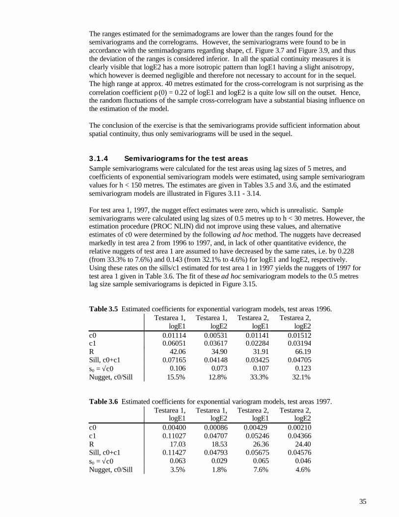
35

The ranges estimated for the semimadograms are lower than the ranges found for thesemivariograms and the correlograms. However, the semivariograms were found to be inaccordance with the semimadograms regarding shape, cf. Figure 3.7 and Figure 3.9, and thusthe deviation of the ranges is considered inferior. In all the spatial continuity measures it isclearly visible that logE2 has a more isotropic pattern than logE1 having a slight anisotropy,which however is deemed negligible and therefore not necessary to account for in the sequel.The high range at approx. 40 metres estimated for the cross-correlogram is not surprising as thecorrelation coefficient ρ(0) = 0.22 of logE1 and logE2 is a quite low sill on the outset. Hence,the random fluctuations of the sample cross-correlogram have a substantial biasing influence onthe estimation of the model.

The conclusion of the exercise is that the semivariograms provide sufficient information aboutspatial continuity, thus only semivariograms will be used in the sequel.

3.1.4 Semivariograms for the test areasSample semivariograms were calculated for the test areas using lag sizes of 5 metres, andcoefficients of exponential semivariogram models were estimated, using sample semivariogramvalues for h < 150 metres. The estimates are given in Tables 3.5 and 3.6, and the estimatedsemivariogram models are illustrated in Figures 3.11 - 3.14.

For test area 1, 1997, the nugget effect estimates were zero, which is unrealistic. Samplesemivariograms were calculated using lag sizes of 0.5 metres up to h < 30 metres. However, theestimation procedure (PROC NLIN) did not improve using these values, and alternativeestimates of c0 were determined by the following ad hoc method. The nuggets have decreasedmarkedly in test area 2 from 1996 to 1997, and, in lack of other quantitative evidence, therelative nuggets of test area 1 are assumed to have decreased by the same rates, i.e. by 0.228(from 33.3% to 7.6%) and 0.143 (from 32.1% to 4.6%) for logE1 and logE2, respectively.Using these rates on the sills/c1 estimated for test area 1 in 1997 yields the nuggets of 1997 fortest area 1 given in Table 3.6. The fit of these ad hoc semivariogram models to the 0.5 metreslag size sample semivariograms is depicted in Figure 3.15.

Table 3.5 Estimated coefficients for exponential variogram models, test areas 1996.Testarea 1,

logE1Testarea 1,

logE2Testarea 2,

logE1Testarea 2,

logE2c0 0.01114 0.00531 0.01141 0.01512c1 0.06051 0.03617 0.02284 0.03194R 42.06 34.90 31.91 66.19Sill, c0+c1 0.07165 0.04148 0.03425 0.04705s0 = √c0 0.106 0.073 0.107 0.123Nugget, c0/Sill 15.5% 12.8% 33.3% 32.1%

Table 3.6 Estimated coefficients for exponential variogram models, test areas 1997.Testarea 1,

logE1Testarea 1,

logE2Testarea 2,

logE1Testarea 2,

logE2c0 0.00400 0.00086 0.00429 0.00210c1 0.11027 0.04707 0.05246 0.04366R 17.03 18.53 26.36 24.40Sill, c0+c1 0.11427 0.04793 0.05675 0.04576s0 = √c0 0.063 0.029 0.065 0.046Nugget, c0/Sill 3.5% 1.8% 7.6% 4.6%

36

0.00

0.02

0.04

0.06

0.08

0.10

0.12

0.14

0 50 100 150 200 250 300

lag h, [metres]

sem

iva

rio

gra

m g

(h)

log E1log E2

Figure 3.11 Sample omni-directional semivariograms and estimated exponentialsemivariogram models for test area 1, Drogden South, 1996.

0.00

0.02

0.04

0.06

0.08

0.10

0.12

0.14

0 50 100 150 200 250 300

lag h, [metres]

sem

iva

rio

gra

m g

(h)

log E1log E2

Figure 3.12 Sample omni-directional semivariograms and estimated exponentialsemivariogram models for test area 2, Flinterenden NW, 1996.

37

0.00

0.02

0.04

0.06

0.08

0.10

0.12

0.14

0 50 100 150 200 250 300

lag h, [metres]

sem

iva

rio

gra

m g

(h)

log E1log E2

Figure 3.13 Sample omni-directional semivariograms and estimated exponentialsemivariogram models for test area 1, Drogden South, 1997.

0.00

0.02

0.04

0.06

0.08

0.10

0.12

0.14

0 50 100 150 200 250 300

lag h, [metres]

sem

iva

rio

gra

m g

(h)

log E1log E2

Figure 3.14 Sample omni-directional semivariograms and estimated exponentialsemivariogram models for test area 2, Flinterenden NW, 1997.

38

0.00

0.02

0.04

0.06

0.08

0.10

0.12

0 5 10 15 20 25 30

logE1logE2

Figure 3.15 Sample omni-directional semivariograms for lag sizes at 0.5 metres, and estimatedexponential semivariogram models for test area 1, Drogden South, 1997, using the ad hocestimated nugget effects.

Based on the semivariogram estimations the following findings were made:

♦ The estimated nugget effects have decreased markedly from 1996 to 1997. The pattern oftest area 1 exhibiting the lower nugget effects is maintained in both years. The nuggeteffects are in concordance with the micro-scale variances found in the backgroundvariability study.

♦ The sills have increased from 1996 to 1997, except for logE2 in test area 2 keeping aconstant sill. The ratios of the sills for logE1 and logE2 in the test areas seem to be stable inboth years, being approx. 2 for test area 1 and 1.2 for test area 2, cf. Figures 3.11 - 3.14.

♦ There is a slightly disturbing decrease in the range values from the 1996 to the 1997datasets. It could be suggested that it is caused by the instationarity observed between 1996and 1997, but it is not possible to give any supporting evidence.

The results are consistent as regards the shape of the spatial continuity function, i.e. thesemivariogram, and with the findings for the bottom type areas, apart for the shrinking of theranges. Thus, as an overall assessment, it is maintained that these semivariogram results areconsistent measures of spatial continuity taking the drift of the signal voltages between 1996and 1997 into account.

39

3.2 Classification of feature spacesFeatures are certain properties expected to enable or enhance the detection of objects of interest.In many image analysis applications the generation and extraction of features is a task in its ownright. For the echo sounder data it could be relevant to conduct a feature extraction exerciseprovided that the full, digitised signal was available. However, it is not; what is at hand is theroughness and hardness features extracted by the RoxAnn device, called E1 and E2. Hence, thefeature space consists of these two variables, and the classification hereof is aimed atestablishing quantitative and computational rules for assigning a sea bottom class to ameasurement Y = (E1, E2)'.

3.2.1 Classification and discriminant analysisModern development of classification algorithms during the last 2 decades has shaped modernadaptive classifiers based on neural networks, deformable templates, and other semiparametricmethods. Several decades before that, classical discriminant analysis based on multivariateGaussian distribution theory and some subsequent nonparametric elaborations were developed.Classical Gaussian discriminant analysis will be employed here, too, leaving modernclassification methods to be pursued in other settings. For a presentation of the application ofdeformable templates to the mussel and sand feature spaces analysed in the sequel, the reader isreferred to Schultz (1995; 1998; 1999) and to her contributions in the BioSonar reports (MAS3-CT95-0026, 1997; 1998; 1999).

An introduction to (multivariate) Gaussian discriminant analysis is given in Conradsen (1984).The classification is based on a statistical discrimination between k Gaussian populations

π1, π2, ..., πk, π i ~ Gaup(µi, Σ i).

To classify an observation x means to assign it to a population π i, which is done by calculating avector u = (u1, ... , uk)' of scores ui for every population by use of

ui(x) = -1/2 log(detSi) - 1/2(x-yi)'Si-1(x-yi) + log(pi), (3.14)

where yi and Si are estimates of the population mean µi and dispersion Σi, and pi is a priorprobability of x being a member of population π i. The observation x is then assigned to the classi for which ui attains the maximum value in the set of ui's. This classification rule is known asthe Bayesian solution, as the posterior probability of x being a member of π i given the value ofx, is

p(π i | x) = exp(ui) / Σ j exp(uj),

thus the maximum ui corresponds to the maximum posterior probability p(π i | x). If priorknowledge is unavailable, i.e. it is not possible to assign reasonable values to pi, the all-equalprinciple is usually used, and the term log(pi) is then removed from (3.14), as all pi are equal.Other classification strategies than the maximisation of posterior probability can be applied, e.g.the minimax (= minimisation of maximum loss) solution choosing a strategy that makes allmisclassification probabilities identical.

In the present feature space there are only two populations, and the third class, the reject class,is comprised of all observations lying outside the two 95% Gaussian confidence ellipsoids. Theuse of the 95% confidence ellipsoids was decided as a compromise between covering thesample populations and securing a minimal overlap of the two confidence ellipsoids.

40

Thereby, the following decision rule for the x assignment applies:

class 0, if ||x-y1||1 > χ²(2)0.95 and ||x-y2||2 > χ²(2)0.95

class 1, if u1(x) > u2(x) and ||x-y1||1 ≤ χ²(2)0.95

class 2, if u1(x) ≤ u2(x) and ||x-y2||2 ≤ χ²(2)0.95,

where the norms ||z||i are given by ||z||i = z'Si-1z. The code 1 is used for the mussel class, and 2 is

used for the sand class.

3.2.2 Estimation of classification regionsThe classification of the mussel and sand feature spaces for 1996 and 1997 was carried out intwo steps. First, a discriminant analysis was carried out based on bigaussian descriptions of themussels and sand samples with different dispersion matrices. Secondly, to introduce a rejectclass describing areas far away from the samples, 95% confidence ellipsoids were used todelimit the mussel and sand classes, leaving the area outside to be classified as an 'other' bottomtype.

In 1996, the two datasets for the mussel and the sand bottom type area contain 709 and 1011observations, respectively. To provide a cross-classification dataset approximately one third ofboth datasets have been put aside for test datasets, leaving 451 and 697 observations for theestimation datasets. Table 3.7 shows the sample averages, y, and dispersions, S, for (log(E1),log(E2))' for the mussels and sand estimation datasets.

Table 3.7 Descriptive statistics for the 1996 estimation datasets (from the bottom type areas)for the bigaussian measurements Y = (logE1, logE2)'.

Mussels , 1996 Sand, 1996

N 451 697

average, y -1.73100 -0.78987

-2.23279 -0.64862

0.01745 0.00350 0.02225 0.00758 dispersion, S 0.00350 0.01540 0.00758 0.03232

The two datasets for the mussel and the sand bottom type areas from 1997 contain 3094 and1624 observations respectively. As for 1996 approximately one third of either dataset havebeen put aside for cross-validation datasets, leaving 2021 and 1126 observations for theestimation dataset. The descriptive statistics for the estimation datasets from 1997 are given inTable 3.8.

Table 3.8 Descriptive statistics for the 1997 estimation datasets for the bigaussianmeasurements Y = (logE1, logE2)'.

Mussels, 1997 Sand, 1997

N 2021 1126

average, y -2.52213 -2.11986

-3.12155 -2.16624

0.04519 0.00704 0.01964 0.00556 dispersion, S 0.00704 0.02110 0.00556 0.04283

41

-3.00

-2.50

-2.00

-1.50

-1.00

-0.50

0.00

-1.50 -1.25 -1.00 -0.75 -0.50 -0.25 0.00

log E2

log

E1

Mussels

Sand

Figure 3.16 (a) The feature space of 1996 with illustrations of the regions used in theclassification: The quadratic border line between the mussel and sand regions, and the 95%approximated confidence ellipsoids for the mussel and sand observations. The separating line,the discriminator curve, is an ellipsoid.

-4.00

-3.50

-3.00

-2.50

-2.00

-1.50

-1.00

-3.00 -2.75 -2.50 -2.25 -2.00 -1.75 -1.50

log E2

log

E1

Mussels

Sand

Figure 3.16 (b) The feature space of 1997 with indications of the regions used in theclassification: The quadratic border line between the mussel and sand regions, and the 95%approximated confidence ellipsoids for the mussel and sand observations. The quadraticdiscriminator function is a hyperbola.

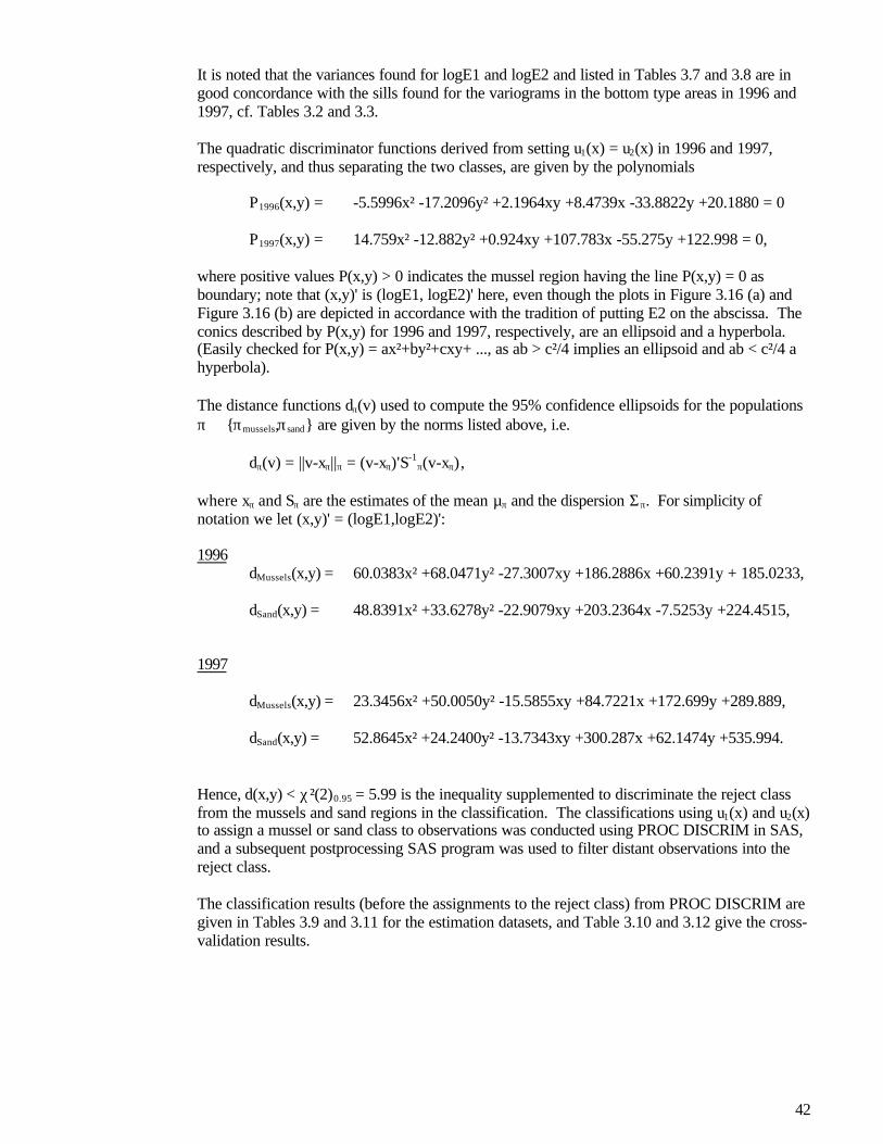
42

It is noted that the variances found for logE1 and logE2 and listed in Tables 3.7 and 3.8 are ingood concordance with the sills found for the variograms in the bottom type areas in 1996 and1997, cf. Tables 3.2 and 3.3.

The quadratic discriminator functions derived from setting u1(x) = u2(x) in 1996 and 1997,respectively, and thus separating the two classes, are given by the polynomials

P1996(x,y) = -5.5996x² -17.2096y² +2.1964xy +8.4739x -33.8822y +20.1880 = 0

P1997(x,y) = 14.759x² -12.882y² +0.924xy +107.783x -55.275y +122.998 = 0,

where positive values P(x,y) > 0 indicates the mussel region having the line P(x,y) = 0 asboundary; note that (x,y)' is (logE1, logE2)' here, even though the plots in Figure 3.16 (a) andFigure 3.16 (b) are depicted in accordance with the tradition of putting E2 on the abscissa. Theconics described by P(x,y) for 1996 and 1997, respectively, are an ellipsoid and a hyperbola.(Easily checked for P(x,y) = ax²+by²+cxy+ ..., as ab > c²/4 implies an ellipsoid and ab < c²/4 ahyperbola).

The distance functions dπ(v) used to compute the 95% confidence ellipsoids for the populationsπ ∈ πmussels,πsand are given by the norms listed above, i.e.

dπ(v) = ||v-xπ||π = (v-xπ)'S-1π(v-xπ),

where xπ and Sπ are the estimates of the mean µπ and the dispersion Σπ. For simplicity ofnotation we let (x,y)' = (logE1,logE2)':

1996dMussels(x,y) = 60.0383x² +68.0471y² -27.3007xy +186.2886x +60.2391y + 185.0233,

dSand(x,y) = 48.8391x² +33.6278y² -22.9079xy +203.2364x -7.5253y +224.4515,

1997

dMussels(x,y) = 23.3456x² +50.0050y² -15.5855xy +84.7221x +172.699y +289.889,

dSand(x,y) = 52.8645x² +24.2400y² -13.7343xy +300.287x +62.1474y +535.994.

Hence, d(x,y) < χ²(2)0.95 = 5.99 is the inequality supplemented to discriminate the reject classfrom the mussels and sand regions in the classification. The classifications using u1(x) and u2(x)to assign a mussel or sand class to observations was conducted using PROC DISCRIM in SAS,and a subsequent postprocessing SAS program was used to filter distant observations into thereject class.

The classification results (before the assignments to the reject class) from PROC DISCRIM aregiven in Tables 3.9 and 3.11 for the estimation datasets, and Table 3.10 and 3.12 give the cross-validation results.

43

Table 3.9 Classification Summary for Calibration Data, 1996.Number of Observations and Percent Classified into CLS:

From CLS To CLS=1 To CLS=2 Total1 449 2 4512 19 678 697

Total 468 680 11481 99.56% 0.44% 100.00%2 2.73% 97.27% 100.00%

Total 40.77% 59.23% 100.00%

Table 3.10 Classification Summary for Cross-validation Data, 1997.Number of Observations and Percent Classified into CLS:


Total 264 308 5721 99.61% 0.39% 100.00%2 2.23% 96.18% 100.00%

Total 46.15% 53.85% 100.00%

Table 3.11 Classification Summary for Calibration Data, 1997.Number of Observations and Percent Classified into CLS:


Total 2020 1127 31471 98.07% 1.93% 100.00%2 3.37% 96.63% 100.00%

Total 64.19% 35.81% 100.00%

Table 3.12 Classification Summary for Cross-validation Data, 1997.Number of Observations and Percent Classified into CLS:


Total 1071 500 15711 98.04% 1.96% 100.00%2 3.82% 96.18% 100.00%

Total 68.17% 31.83% 100.00%

The cross-validation results given in Tables 3.10 and 3.12 supplemented by the contents ofFigures 3.17 and 3.18, showed that the results of the classification of the feature space are fairlyrobust and reliable. Feature space inspection and the estimated variogram models underpin thefinding that the magnitude of the E1 and E2 values cannot be used directly in a reliableestimation procedure, wherefore it is recommendable to use the classification method describedhere in an adaptive fashion.

44

-3.00

-2.50

-2.00

-1.50

-1.00

-0.50

-1.25 -1.00 -0.75 -0.50 -0.25 0.00

log E2

log

E1

Mussels

Sand

Figure 3.17 The rejects and misclassified observations from the bottom type areas of 1996, 36observations from the sand area and 36 from the mussel area.

-3.50

-3.00

-2.50

-2.00

-1.50

-1.00

-2.75 -2.50 -2.25 -2.00 -1.75 -1.50

log E2

log

E1

Mussels

Sand

Figure 3.18 The rejects and misclassified observations from the bottom type areas of 1997, 109observations from the sand area and 201 from the mussel area.

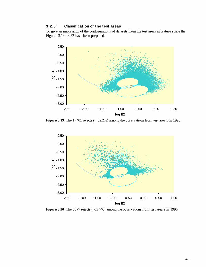
45

3.2.3 Classification of the test areasTo give an impression of the configurations of datasets from the test areas in feature space theFigures 3.19 - 3.22 have been prepared.

-3.00

-2.50

-2.00

-1.50

-1.00

-0.50

0.00

0.50

-2.50 -2.00 -1.50 -1.00 -0.50 0.00 0.50

log E2

log

E1

Figure 3.19 The 17401 rejects (~ 52.2%) among the observations from test area 1 in 1996.

-3.00

-2.50

-2.00

-1.50

-1.00

-0.50

0.00

0.50

-2.50 -2.00 -1.50 -1.00 -0.50 0.00 0.50 1.00

log E2

log

E1

Figure 3.20 The 6877 rejects (~22.7%) among the observations from test area 2 in 1996.

46

-4.00

-3.50

-3.00

-2.50

-2.00

-1.50

-1.00

-0.50

0.00

-3.25 -2.75 -2.25 -1.75 -1.25 -0.75

log E2

log

E1

Figure 3.21 The 35468 rejects (~ 45.9%) among the observations from test area 1 in 1997.

-4.00

-3.50

-3.00

-2.50

-2.00

-1.50

-1.00

-0.50

0.00

-3.25 -2.75 -2.25 -1.75 -1.25 -0.75

log E2

log

E1

Figure 3.22 The 1623 rejects (~15.5%) among the observations from test area 2 in 1997.

Table 3.13 Classification summary for the test areas in 1996 and 1997.frequency percent

mussels sand reject mussels sand reject1996, test area 1 13109 2640 17401 39.5 8.0 52.51996, test area 2 22849 521 6877 75.5 1.7 22.71997, test area 1 39299 2481 35468 50.9 3.2 45.91997, test area 2 8747 76 1623 83.7 0.7 15.5

47

The classification results for the test areas are summarised in Table 3.13. Very small fractionsof the observations are classified as sand, whereas the mussels as expected are clearly dominantin test area 2, which is also reflected by Figure 3.20 and 3.22. In test area 1 the expectedheterogeneous pattern is mirrored in the feature space.

3.2.4 InterpretationsA word on the interpretation of the feature space classification is in place. The interpretationoffered in this thesis is conservative as it uses a binary scale for assigning mussel or sand classesto the observations. Several like studies operate with trinary or quaternary scales, the trinaryscale containing a class corresponding to the middle gray region of undecidedness (50/50), andthe quarternary scale using 4 classes corresponding to the quartile intervals of 0-25%, 26-50%,etc. However, here the aim is to lay a reliable corner stone for future developments, and as longas there is no supporting evidence that warrants further divisions of the mussel-sand scale it willnot be discussed here.

Other approaches could be envisioned, e.g. an approach using the Mahalanobis distances froman observation to the sample averages of the mussel and sand populations in feature space toassign a probability vector to the observation by inverting the quantile of the correspondingcontour line into a probability. However, such approaches can only be qualified by certaintypes of datasets, e.g. bottom type areas having a fixed coverage rate of mussels below 100%,and as these are not at hand, it will be superfluous to embark on such a venture here.

What is really at stake is the challenge of identifying (link) functions µ(c;θ) and e(c;ψ) for therelation between RoxAnn measurements Z(s) = (E1(s), E2(s))' and the mussel coverage ratec(s) at the location s:

Z(s) = (E1(s), E2(s))' = µ(c(s);θ) + e(c(s);ψ)

where θ and ψ are auxiliary parameters describing other properties that the mean field and thesmall-scale variation might depend upon, like the pattern of the mussels, e.g. patches or smoothtexture. Even in a very simple form,

Z(s) = µ(c(s)) + e(s) (3.15)

this functional relation is not identifiable from the datasets produced during the BioSonar fieldcampaigns. Based on the existing datasets the following statistics of the function (3.15) wereestimated:

E(Z(s) | c ≈ 0) and V(Z(s) | c ≈ 0)and

E(Z(s) | c ≈ 1) and V(Z(s) | c ≈ 1)

for the sand and mussel bottom type areas, respectively. That is, knowledge about the functionat the endpoints of the coverage rate scale has been obtained (and it was found that theseendpoints seem to be instationary although maintaining the same relative positions in featurespace). Future scrutiny of the function µ(c;θ) could involve tank experiments with controlled /designed mussel textures, which would be very interesting.

48

3.3 Preparation of distribution maps and estimates ofdistribution areas

This section describes in detail how the calculated variograms and classified regions of featurespace are used intertwined to produce spatial distribution maps by kriging of the observationsfollowed by classification of the kriged values.

3.3.1 Validation maps for the bottom type areasFor the bottom type areas spatial distribution maps have been prepared mainly to validate theuse of the classification rule given in section 3.3. It is expected that they will reflect thepresence of a homogeneous sea bottom covered either by mussels or sand.

The distribution maps were prepared in a simple and straightforward fashion by kriging theobservations of logE1 and logE2 to estimate point values on a grid where points are separatedby 1 metre in vertical and horizontal directions. The kriging was based on the variogrammodels given by the coefficients listed in Tables 3.2 and 3.3. The maps were produced usingSurfer, version 6.0, and the grids containing the results of the point kriging were postprocessedwith a SAS program to provide the classified maps using the classification rule given in section3.3. The resulting classification codes are given as:

1 ~ mussels, 2 ~ sand, and 0 ~ reject class.

The mussel codes are depicted as blue (the darker colour in gray scale), the sand codes areyellow (the lighter colour in gray scale), and the reject codes are white throughout this section.The resulting maps are depicted in Figures 3.23 - 3.26, where the kriged map of the water depthhas been included to allow scrutiny of potential deviations, etc.

364800 364850 364900

6162050

6162100

6162150

-2.20

-2.00

-1.80

-1.60

-1.40

-1.20

364800 364850 364900

6162050

6162100

6162150

-1.50

-1.30

-1.10

-0.90

-0.70

-0.50

364800 364850 364900

6162050

6162100

6162150

0.00

1.00

2.00

364800 364850 364900

6162050

6162100

6162150

4.50

4.70

4.90

5.10

5.30

5.50

5.70

5.90

Figure 3.23 Mussel bottom type area, 1996. LogE1 is mapped upper left, logE2 is mappedupper right, depth is mapped lower right, and lower left depicts the classified distribution map.

49

357640 357660 357680 357700 357720

6162380

6162400

6162420

6162440

6162460

-2.50

-2.30

-2.10

-1.90

-1.70

357640 357660 357680 357700 357720

6162380

6162400

6162420

6162440

6162460

-1.00

-0.80

-0.60

-0.40

357640 357660 357680 357700 357720

6162380

6162400

6162420

6162440

6162460

0.00

1.00

2.00

357640 357660 357680 357700 357720

6162380

6162400

6162420

6162440

6162460

4.00

4.20

4.40

4.60

4.80

5.00

Figure 3.24 Sand bottom type area, 1996. LogE1 is mapped upper left, logE2 is mapped upperright, depth is mapped lower right, and lower left depicts the classified distribution map.

364800 364850 364900

6162050

6162100

6162150

-3.00

-2.60

-2.20

-1.80

-1.40

364800 364850 364900

6162050

6162100

6162150

-2.70

-2.30

-1.90

-1.50

364800 364850 364900

6162050

6162100

6162150

0.00

1.00

1.50

2.00

3.00

364800 364850 364900

6162050

6162100

6162150

3.75

4.25

4.75

5.25

Figure 3.25 Mussel bottom type area, 1997. LogE1 is mapped upper left, logE2 is mappedupper right, depth is mapped lower right, and lower left depicts the classified distribution map.

50

357635 357660 357685 357710 3577356162370

6162395

6162420

6162445

6162470

-3.50

-3.30

-3.10

-2.90

-2.70

-2.50

357635 357660 357685 357710 3577356162370

6162395

6162420

6162445

6162470

-2.70

-2.50

-2.30

-2.10

-1.90

-1.70

-1.50

357640 357660 357680 357700 357720

6162380

6162400

6162420

6162440

6162460

0.00

1.00

2.00

357635 357660 357685 357710 3577356162370

6162395

6162420

6162445

6162470

3.50

3.70

3.90

4.10

4.30

4.50

Figure 3.26 Sand bottom type area, 1997. LogE1 is mapped upper left, logE2 is mapped upperright, depth is mapped lower right, and lower left depicts the classified distribution map.

A short summary of the classification results for the kriged points is given in Table 3.14. Thefollowing observation can be made in Figures 3.23 - 3.26 and Table 3.14:

♦ The 1996 maps of logE1 and logE2 appear smoother than the maps for 1997, which is aneffect of the lower data density and the lower transect density.

♦ In the 1997 maps the data along transects are clearly reflected in the kriged maps, whereforeit could be argued that the side length of the square grid cells should have been greater (than1 metres) for the 1997 data. This is particularly apparent in the maps of the water depths;however, the grid cell size being identical in both years allows comparisons to be madewithout qualifications regarding differences in cell size.

♦ The patterns of the depth maps, i.e. the topography, are reproduced fairly well from 1996 to1997, which is a good underpinning of the validity of the data.

♦ Mussels are represented as a strong majority in the mussel bottom type area, and sand isvice versa in the sand areas. The positions and number of blank spots containingcomplementary bottom classes are not reproduced from 1996 to 1997, which can beattributed to random variation inherent in the measurement process, or, at least in themussels case, a result of restructuring of mussel beds, i.e. wandering and settling ofmussels.

51

Table 3.14 A summary of the classification of the kriged values for the bottom type areas,given in percentages of the total number of grid points.

Mussels Sand Reject TotalMussels, 1996 99.4 0.0 0.6 100.0Mussels, 1997 98.6 0.2 1.2 100.0Sand, 1996 0.3 99.7 0.0 100.0Sand, 1997 0.6 98.9 0.5 100.0

Regardless, the main observation is that the fractions of grid points classified as mussels in themussel area and those classified as sand in the sand area, given in Table 3.14, seem prettyconvincing and provide a proper validation of the outlined classification scheme. The classifiedmaps evidently support this impression.

3.3.2 Distribution maps for test area 1, Drogden SouthThe maps of the spatial distribution of mussels should provide this information lending itself toclear and unambiguous interpretation. Thus, the following considerations applied to the methodchosen for preparing the maps. It is considered desirable, that the maps depicted in rasterformat contain directly interpretable figures, hence every pixel should represent an average ofthe part of the region it covers. In other words block kriging is more suited for this task thanpoint kriging.

For the block kriging a discretisation of the pixel interior by use of 4 x 4 points was chosen onthe basis of the recommendation by given Isaaks & Srivastava (1989), where 4 x 4 points isrecommended as a minimum limit for ensuring stability of the results. One way to go about thiswould be to form block averages directly from the 4 x 4 values obtained from point kriging andthen classifying the block averages using a modified dispersion matrix S adjusted for theaveraging of 16 spatially dependent point estimates from Z(s). Alternatively, the variogrammodel could be adjusted for the change of support from points to the pixel blocks and then usedin a "point" kriging that would produce the block averages directly. Journel & Huijbregts(1978) give a thorough discussion of how to adjust variogram models for change of support.

Either way, the result will be a binary variable, and therefore a hybrid approach was chosen togain a little more resolution. Thus, an ordinary point kriging system is used to estimate the 16points, which are then classified individually. Afterwards, mussel and sand proportions arecalculated as the marginal ratios hereof within every pixel. The classification rule for the blockis set to use a 50% thresholding rule, i.e. if one of the proportions pmus or psand are greater than0.5, the pixel will be classified accordingly, otherwise it will be assigned to the reject class.Suppose c is a 16-valued vector containing the classification results ci at all the 4 x 4 subgridpoints, then pmus, psand and class are assigned values as follows:

pmus = Σi=1..16 I[ci=<mussels>]/16

psand = Σi=1..16 I[ci=<sand>]/16

class = <mussels>, if pmus > 0.5<sand>, if psand > 0.5<reject>, otherwise.

If pmus = psand = 0.5 a coin is flipped (this didn't occur anywhere).

Other considerations concern the choice of pixel size in the grid to be used. An upper limit isindicated by the magnitude of the range of influence, R. Hence, going substantially higher thanR a very smoothed result can be expected as then the spatial continuity is smoothed at the globallevel, and thus will be close to the overall kriged average. As a rule-of-thumb a lower limit is

52

set by the minimum distance between data, as the purpose of kriging is to estimate the meanfield by smoothing out small-scale spatial variation which cannot be observed below theminimum distance between observations. Sometimes a similar concern is phrased as "the dataare visible in the kriged map", not implying the obvious, but rather that deviating small-scalepatterns are seen in regions of high data density; an observation like that would indicate that thegrid size should be increased. These concerns have been combined with a rationale of keeping afixed relative data density thereby making use of the three distinct grid sizes used in thesampling of the areas to obtain maps in various scales of resolution. Thus, maps have beenprepared for the total outstretch of the test areas having gross transect distances at 120 metresusing the hybrid block kriging and proportion calculation of pixels at 30 x 30 m² pixels. For thecenter part of the test areas containing transects 60 metres apart the size of the pixels werechosen at 15 x 15 m², and for the core part of test area 1 where transects are 20 metres apart thepixel size was chosen at 5 x 5 m². Thus, the relative data density is maintained (approximately)by choosing pixel sizes at a ratio 30: 15: 5 similar to the transect distances at 120: 60: 20.

The specifications of the geographic boundaries for the maps prepared for test area 1 are givenin Table 3.15.

Table 3.15 Specifications of the geographic boundaries for the total area and subareas in testarea 1, Drogden South.

Areaside length ofsquare pixels /m

map boundaries in UTMcoordinates

image dimensions(height x width)

Total area 30 [355520, 357200] x[6162000, 6163440]

48 x 56

Center area withtransects 60 m apart

15 [355700, 356330] x[6162420, 6163050]

42 x 42

Core part withtransects 20 m apart

5 [355940, 356060] x[6162680, 6162800]

24 x 24

356000 356500 357000

6162250

6162750

6163250

-2.50

-2.00

-1.50

-1.00

-0.50

356000 356500 357000

6162250

6162750

6163250

-2.00

-1.50

-1.00

-0.50

0.00

356000 356500 3570006162000

6162500

6163000

356000 356500 357000

6162250

6162750

6163250

2.00

3.00

4.00

5.00

6.00

7.00

8.00

Figure 3.27 Kriged observation maps and the distribution map containing classified 30 x 30 mblocks for test area 1, 1996. LogE1 is mapped upper left, logE2 upper right, and depth lowerright. The lower left depicts the classified distribution map, where blue is mussels and yellow issand.

53

356000 356500 357000

6162500

6163000

0.00

0.20

0.40

0.60

0.80

1.00

356000 356500 357000

6162500

6163000

0.00

0.20

0.40

0.60

0.80

1.00

356000 356500 357000

6162500

6163000

Figure 3.28 Maps for the total test area mainly covered by transects 120 metres apart, for testarea 1, 1996. At the top the mussel proportions map is depicted, the middle depicts the sandproportions map, and the lower is the classified map. The total area is 1680 x 1440 m² = 2.4192km².

54

355800 356000 356200

6162600

6162800

6163000

355800 356000 356200

6162600

6162800

6163000

Figure 3.29 Maps for the centered area covered by 60 metres interspersed transects, for testarea 1, 1996. The left map shows the mussel proportions, and the right contains the classifiedmap. The total area is 630 x 630 m² = 0.3969 km².

355950 356000 356050

6162700

6162750

355950 356000 356050

6162700

6162750

Figure 3.30 Maps for the core area covered by transects 20 metres apart, for test area 1, 1996.The left map contains the mussel proportions, and the right map holds the classified map. Thetotal area is 120 x 120 m².

The block kriging was carried out using Surfer to prepare the point kriging results on the 4 x 4subgrids, followed by a calculation of the proportions within blocks and the block class using aSAS program. The results are pixels of 900 m², 225 m² and 25 m² having assigned values of asea bottom class, and assigned proportions of mussel and sand coverage rates in a resolution ofunity at 2-4, i.e. 0, 1/16, 2/16, ..., 1.

The maps for logE1, logE2 and depth contained in Figure 3.27 and 3.31 were prepared usingpoint kriging to a 10 metres grid. This was done to give an indication of their patterns of spatialvariation at a higher resolution than provided by the 30 m grid.

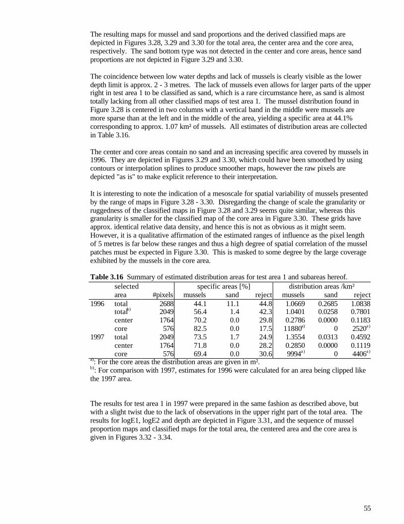
55

The resulting maps for mussel and sand proportions and the derived classified maps aredepicted in Figures 3.28, 3.29 and 3.30 for the total area, the center area and the core area,respectively. The sand bottom type was not detected in the center and core areas, hence sandproportions are not depicted in Figure 3.29 and 3.30.

The coincidence between low water depths and lack of mussels is clearly visible as the lowerdepth limit is approx. 2 - 3 metres. The lack of mussels even allows for larger parts of the upperright in test area 1 to be classified as sand, which is a rare circumstance here, as sand is almosttotally lacking from all other classified maps of test area 1. The mussel distribution found inFigure 3.28 is centered in two columns with a vertical band in the middle were mussels aremore sparse than at the left and in the middle of the area, yielding a specific area at 44.1%corresponding to approx. 1.07 km² of mussels. All estimates of distribution areas are collectedin Table 3.16.

The center and core areas contain no sand and an increasing specific area covered by mussels in1996. They are depicted in Figures 3.29 and 3.30, which could have been smoothed by usingcontours or interpolation splines to produce smoother maps, however the raw pixels aredepicted "as is" to make explicit reference to their interpretation.

It is interesting to note the indication of a mesoscale for spatial variability of mussels presentedby the range of maps in Figure 3.28 - 3.30. Disregarding the change of scale the granularity orruggedness of the classified maps in Figure 3.28 and 3.29 seems quite similar, whereas thisgranularity is smaller for the classified map of the core area in Figure 3.30. These grids haveapprox. identical relative data density, and hence this is not as obvious as it might seem.However, it is a qualitative affirmation of the estimated ranges of influence as the pixel lengthof 5 metres is far below these ranges and thus a high degree of spatial correlation of the musselpatches must be expected in Figure 3.30. This is masked to some degree by the large coverageexhibited by the mussels in the core area.

Table 3.16 Summary of estimated distribution areas for test area 1 and subareas hereof.specific areas [%] distribution areas /km²selected

area #pixels mussels sand reject mussels sand reject1996 total 2688 44.1 11.1 44.8 1.0669 0.2685 1.0838

totalb) 2049 56.4 1.4 42.3 1.0401 0.0258 0.7801center 1764 70.2 0.0 29.8 0.2786 0.0000 0.1183core 576 82.5 0.0 17.5 11880a) 0 2520a)

1997 total 2049 73.5 1.7 24.9 1.3554 0.0313 0.4592center 1764 71.8 0.0 28.2 0.2850 0.0000 0.1119core 576 69.4 0.0 30.6 9994a) 0 4406a)

a): For the core areas the distribution areas are given in m².b): For comparison with 1997, estimates for 1996 were calculated for an area being clipped likethe 1997 area.

The results for test area 1 in 1997 were prepared in the same fashion as described above, butwith a slight twist due to the lack of observations in the upper right part of the total area. Theresults for logE1, logE2 and depth are depicted in Figure 3.31, and the sequence of musselproportion maps and classified maps for the total area, the centered area and the core area isgiven in Figures 3.32 - 3.34.

56

356000 356500 357000

6162250

6162750

6163250

-3.00

-2.50

-2.00

-1.50

-1.00

-0.50

0.00

356000 356500 357000

6162250

6162750

6163250

-2.75

-2.50

-2.25

-2.00

-1.75

-1.50

-1.25

356000 356500 3570006162000

6162500

6163000

356000 356500 357000

6162500

6163000

2.50

3.50

4.50

5.50

6.50

Figure 3.31 Kriged observation maps and the distribution map containing classified 30 x 30 mblocks for test area 1, 1997. LogE1 is mapped upper left, logE2 upper right, and depth lowerright. The lower left depicts the classified distribution map, where blue is mussels and yellow issand.

The coincidence between low water depths and lack of mussels cannot be reproduced in the1997 maps due to the lack of data in the upper right. However, in the vicinity of the upper rightsloped edge bordering to that part of the area, there are traces of sand in the classified map inFigure 3.32. The general pattern of the mussel distribution found in 1996, cf. Figure 3.28, isreproduced to some extent, i.e. the description of the mussel distribution centered in twocolumns with a sparser vertical band in the middle still applies. The 1997 map indicates that themussels have spread into the southern part of the area, indicating a general increase in theabundance of mussels in test area 1, from 1996 to 1997. The corresponding estimates of musseldistribution area are 1.04 km² and 1.36 km² for 1996 and 1997, respectively, corresponding toan increase in specific area from 56.4% to 73.5%, cf. Table 3.16.

The indication of a (meso-)scale for spatial variability of mussels discussed for the 1996 maps isvisible for the 1997 maps too. In 1997 the mussel distribution in the core area, cf. Figure 3.34,has decreased markedly compared to 1996, from 82.5% to 69.4% measured by the specific area.Most of the blank spots from the 1996 core area map, cf. Figure 3.30, are recaptured by the1997 map of the core area, and many more blank spots have appeared in the meantime,indicating that an erosion of the mussel beds in the area has taking place.

57

356000 356500 357000

6162500

6163000

0.00

0.20

0.40

0.60

0.80

1.00

356000 356500 357000

6162500

6163000

0.00

0.20

0.40

0.60

0.80

1.00

356000 356500 3570006162000

6162500

6163000

Figure 3.32 Maps for the total test area mainly covered by transects 120 metres apart, for testarea 1, 1997. At the top the mussel proportions are depicted, the middle contains the sandproportions map, and at the bottom the classified map is depicted. The total area is 1680 x 1440m² - 1040 x (280+820)/2 m² = 1.8472 km², and the pixel size is 30 x 30 m².

58

355800 356000 356200

6162600

6162800

6163000

355800 356000 356200

6162600

6162800

6163000

Figure 3.33 Maps for the centered area covered by transects 60 metres apart, for 1997. The leftmap shows the mussel proportions, and the right the classified map obtained by thresholding theleft map at 0.5. The total area is 630 x 630 m² = 0.3969 km², and the pixel size is 15 x 15 m².

355950 356000 356050

6162700

6162750

355950 356000 356050

6162700

6162750

Figure 3.34 Maps for the core area covered by transects 20 metres apart. The left map showsthe mussel proportions, and the right map contains the classified map. The total area is 120 x120 m², and the pixel size is 5 x 5 m².

3.3.3 Distribution maps for test area 2, Flinterenden NWDistribution maps for test area 2 in 1996 and 1997 have been prepared by the same method asdescribed for test area 1 above, i.e. using square pixels with a side length of 30 metres to form ahybrid block kriging of mussel and sand proportions. The distribution maps for test area 2 in1996 are depicted in Figures 3.35, 3.36 and 3.37, indicating huge amounts of mussels at theseabed. In particular, the degree of pixels having coverage rates at 100% or just below 100% isremarkable in Figure 3.36, indicating a large and homogeneous mussel bed in the area. At theupper western edge the depth delimitation of the mussels is reflected.

59

In 1997, having confirmed the abundant distribution of mussels in test area 2, the fieldcampaign was redesigned to put emphasis on more interesting matters than monitoring large,homogeneous patches of mussels, cf. Figure 3.36. Thus, only the core part of the area wassampled in 1997. To enable some comparison between 1996 and 1997 the core part of the areawas mapped for 1996 as well using square pixels with a side length at 15 metres. The estimateddistribution areas and specific areas are given in Table 3.17.

Table 3.17 Estimates of distribution areas in test area 2.selected specific area distribution area /m²area reject mussels sand reject mussels sand

1996 total 2448 18.1 81.8 0.1 398779 1802218 2203core 595 0.2 99.8 0 268 133607 0

1997 core 595 2.9 97.1 0 3882 129993 0

In the specific areas given in Table 3.17 the abundant mussel beds in test area 2 are evident, andeven more so in the core part of the areas in 1996 and 1997 having specific areas at 99.8% and97.1%, barely a decrease worth mentioning. However, although the majority of the averagecoverage rates obtained for the 15 x 15 m² pixels in the maps in Figures 3.38 and 3.39 aregreater than 0.5, there is a visible tendency in the mussel proportions maps of some decreases inthe coverage rates.

362000 362500 363000 3635006162000

6162500

6163000

6163500

-2.00

-1.50

-1.00

-0.50

0.00

362000 362500 363000 3635006162000

6162500

6163000

6163500

-2.00

-1.60

-1.20

-0.80

-0.40

0.00

362000 362500 363000 363500

6162000

6162500

6163000

6163500

6164000

362000 362500 363000 3635006162000

6162500

6163000

6163500

1.00

3.00

5.00

7.00

Figure 3.35 Distribution map for test area 2, 1996. LogE1 is mapped upper left, logE2 ismapped upper right, depth is mapped lower right, and lower left depicts the classifieddistribution map.

60

362000 362500 363000 363500

6162000

6162500

6163000

6163500

6164000

0.00

0.20

0.40

0.60

0.80

1.00

362000 362500 363000 363500

6162000

6162500

6163000

6163500

6164000

Figure 3.36 Maps for test area 2 in 1996 mainly covered by transects 120 metres apart. Theupper map depicts the mussel proportions, and the lower is the corresponding classified map.The total area is 2.2032 km², and the pixel size is 30 x 30 m².

61

362600 362700 362800 362900 363000

6162800

6162900

6163000

6163100

6163200

-3.00

-2.50

-2.00

-1.50

-1.00

362600 362700 362800 362900 363000

6162800

6162900

6163000

6163100

6163200

-3.00

-2.50

-2.00

-1.50

-1.00

362600 362700 362800 362900 363000

6162800

6162900

6163000

6163100

6163200

362600 362700 362800 362900 363000

6162800

6162900

6163000

6163100

6163200

3.50

4.50

5.50

6.50

Figure 3.37 Distribution map for test area 2, 1997. LogE1 is mapped upper left, logE2 ismapped upper right, depth is mapped lower right, and lower left depicts the classifieddistribution map.

62

362600 362700 362800 362900 363000

6162800

6162900

6163000

6163100

6163200

362600 362700 362800 362900 363000

6162800

6162900

6163000

6163100

6163200

Figure 3.38 Maps for the core part of test area 2, 1996, mainly covered by transects 60 and 20metres apart. The left map depicts the mussel proportions, and at the right the classified map isdepicted. The total area is 0.1339 km², and the pixel size is 15 x 15 m².

362600 362700 362800 362900 363000

6162800

6162900

6163000

6163100

6163200

362600 362700 362800 362900 363000

6162800

6162900

6163000

6163100

6163200

Figure 3.39 Maps for (the core part of) test area 2, 1997, mainly covered by transects 60 and20 metres apart. The left map depicts the mussel proportions, and at the right the classified mapis depicted. The total area is 0.1339 km², and the pixel size is 15 x 15 m².

63

3.4 Change detection in mussel distribution mapsThis section illustrates a few heuristic ways of assessing the changes in mussel distributionbased on the maps presented in section 3.3. Some common sense basics of spatial changedetection and related hypothesis testing is discussed in Martin & Scott (1995).

One of the objectives of the BioSonar project has been to study the opportunities for changedetection in the developed map preparation and data processing methodology. Theseopportunities can be illustrated by use of the observations recorded for test area 1, DrogdenSouth, in Øresund. Having employed the thorough data processing scheme described anddeveloped in the preceding sections one finally arrives at maps depicting locations of mussels,sand and the so-called reject class, representing all other bottom types. On the basis of thesedistribution maps it is elementary to subtract the maps of 1996 from those of 1997 to formdifference maps, which have been done for test area 1 in total, for the center area, and for thecore part. The resulting maps are depicted in Figures 3.40, 3.41 and 3.42, respectively, alongwith the distribution maps of 1996 and 1997.

As noted above it seems that the mussels have been increasing their abundance in the southernpart of the area while maintaining large parts of their distribution in particular in the center ofthe total area bordering to the sloping edge at the upper right. To assess whether the expectedcorrelation between the locations of sea bottom classes of 1996 and 1997 is present, a 2-wayfrequency table was generated using SAS, cf. Table 3.18. A χ²-test was used to test whether thecontents of the table can be assumed to be random, i.e. that the pixels of 1996 are independentof the pixels in 1997. The test result shown in the lower part of Table 3.18 strongly indicatesthat this is not the case here, and that indeed the pixels classified as mussels in 1996 to a largeextent are classified as mussels in 1997 too, and vice versa.

The postulated spread of mussels in the southern part of the area in 1997 was quantifiedlikewise by separating the area into a northern and a southern part at UTM Northings of6162700, and then producing the 2-way tables in each part of the area. The results are depictedin Table 3.19 and show that the migration between the reject and mussel classes is about equalin the northern part, as 164 mussel pixels have vanished and 140 new mussel pixels haveappeared in 1997. In the southern part, there is a marked increase in the number of musselpixels, 46 have gone and 416 new mussel pixels have appeared, strongly underlining the visualimpression of the distribution maps and their changes.

64

356000 356500 3570006162000

6162500

6163000

356000 356500 3570006162000

6162500

6163000

356000 356500 3570006162000

6162500

6163000

Figure 3.40 Graphical change detection for test area 1. In the map at the bottom, red (thedarker colour in grayscale prints) is the color of decreases from 1996 to 1997, and green (thelighter colour) indicates increases from 1996 to 1997. At the top, the 1996 distribution map isdepicted, in the middle the 1997 map is shown.

65

355800 356000 356200

6162600

6162800

6163000

355800 356000 356200

6162600

6162800

6163000

355800 356000 356200

6162600

6162800

6163000

Figure 3.41 Graphical change detection for the center part of test area 1 containing transects 60metres apart, illustrated by the classified maps. In the map at the bottom, red (the darker colourin grayscale prints) is the color of decreases from 1996 to 1997, and green (the lighter colour)indicates increases from 1996 to 1997. At the top, the 1996 distribution map is depicted, in themiddle the 1997 map is shown.

66

355950 356000 356050

6162700

6162750

355950 356000 356050

6162700

6162750

355950 356000 356050

6162700

6162750

Figure 3.42 Graphical change detection for the core part of test area 1 containing transects 20metres apart, illustrated by the mussel proportion maps. In the map at the bottom, red (thedarker colour in grayscale prints) is the color of decreases from 1996 to 1997, and green (thelighter colour) indicates increases from 1996 to 1997. At the top, the 1996 distribution map isdepicted, in the middle the 1997 map is shown.

67

Table 3.18 A categorical table of the classified pixels in the clipped test area 1 in 1997 versusthe classes in 1996 (output from PROC FREQ in SAS) for the same pixels. A χ²-test of cellindependence is included in the lower part of the table.

TABLE OF CLS97 BY CLS96

CLS97 CLS96

Frequency‚ Percent ‚ Row Pct ‚ Col Pct ‚ 0‚ 1‚ 2‚ Total ƒƒƒƒƒƒƒƒƒˆƒƒƒƒƒƒƒƒˆƒƒƒƒƒƒƒƒˆƒƒƒƒƒƒƒƒˆ 0 ‚ 290 ‚ 210 ‚ 10 ‚ 510 ‚ 14.15 ‚ 10.25 ‚ 0.49 ‚ 24.89 ‚ 56.86 ‚ 41.18 ‚ 1.96 ‚ ‚ 33.49 ‚ 18.18 ‚ 35.71 ‚ ƒƒƒƒƒƒƒƒƒˆƒƒƒƒƒƒƒƒˆƒƒƒƒƒƒƒƒˆƒƒƒƒƒƒƒƒˆ 1 ‚ 556 ‚ 941 ‚ 8 ‚ 1505 ‚ 27.14 ‚ 45.92 ‚ 0.39 ‚ 73.45 ‚ 36.94 ‚ 62.52 ‚ 0.53 ‚ ‚ 64.20 ‚ 81.47 ‚ 28.57 ‚ ƒƒƒƒƒƒƒƒƒˆƒƒƒƒƒƒƒƒˆƒƒƒƒƒƒƒƒˆƒƒƒƒƒƒƒƒˆ 2 ‚ 20 ‚ 4 ‚ 10 ‚ 34 ‚ 0.98 ‚ 0.20 ‚ 0.49 ‚ 1.66 ‚ 58.82 ‚ 11.76 ‚ 29.41 ‚ ‚ 2.31 ‚ 0.35 ‚ 35.71 ‚ ƒƒƒƒƒƒƒƒƒˆƒƒƒƒƒƒƒƒˆƒƒƒƒƒƒƒƒˆƒƒƒƒƒƒƒƒˆ Total 866 1155 28 2049 42.26 56.37 1.37 100.00

STATISTICS FOR TABLE OF CLS97 BY CLS96

Statistic DF Value Prob ƒƒƒƒƒƒƒƒƒƒƒƒƒƒƒƒƒƒƒƒƒƒƒƒƒƒƒƒƒƒƒƒƒƒƒƒƒƒƒƒƒƒƒƒƒƒƒƒƒƒƒƒƒƒ Chi-Square 4 285.696 0.001 Likelihood Ratio Chi-Square 4 139.801 0.001 Mantel-Haenszel Chi-Square 1 48.634 0.001 Phi Coefficient 0.373 Contingency Coefficient 0.350 Cramer's V 0.264

Sample Size = 2049

68

Table 3.19 Categorical tables of classified pixels from 1997 versus classified pixels from 1996,for the northern part (UTM Northing above 6162700) of test area 1 (the upper table) and thesouthern part of test area 1 (the lower table).


CLS97 CLS96



CLS97 CLS96


69

3.5 Groundtruthing and verificationHaving all the prepared distribution maps at hand it is stimulating to turn to reality for a while.In the following a small selection of the groundtruth data is presented, with a primary focus onthe sea bottom imagery obtained during the field campaigns.

7a: (364822, 6162142) 7b: (364822, 6162142)

8a: (364829, 6162149) 8b: (364829, 6162149)

Figure 3.43 Groundtruthing photos from the mussel bottom type area, taken at the upper leftrim of the area. Locations 7 and 8 were classified as mussels.

For the bottom type areas the photos taken at the bottom fulfilled the expectations of a smoothand homogeneous bottom coverage of mussels and sand, respectively. Figure 3.43 depictsphotos taken at the locations 7 and 8 in the mussel bottom type area and the mussels are clearlyabundant in these locations. All photos were made in duplicate by lowering the photo samplertwice through the water column onto the seafloor. Differences in duplicate photos are causedby the drift of the vessel in the time interval between the two photos were taken.

The size of the bottom covered by the photo sampler is approx. 2 m², which is quite close to thepixel size used for the bottom type areas, whereas for the test areas the basic pixel size is 30 x30 m². Hence, the photos can merely give indications of the sea floor in their closesurroundings in the test areas, wherefore it would be preferable to have a selection procedure forthe groundtruthing sites that could adapt to proposed pixel sizes for the resulting maps. Thesecould in turn be derived from investigations of spatial continuity based on preliminaryinvestigations. Having a proposed pixel size at hand photos could be recorded in selected pixelsat all of the 4 x 4 discretisation points used for block kriging.

70

12a: (356908, 6162320) 12b: (356908, 6162320)

13a: (356311, 6162078) 13b: (356311, 6162078)

16a: (355589, 6162316) 16b: (355589, 6162316)

22a: (356048, 6163407) 22b: (356048, 6163407)

Figure 3.44 Selected groundtruthing photos from test area 1, 1996. The locations 12, 13 and22 were classified as rejects, i.e. neither mussels nor sand, and the location 16 was classified asa mussel seafloor, cf. Figure 3.28.

71

In Figure 3.44 a selection of photos from test area 1 in 1996 is shown. Three of the fourlocations depicted are classified as rejects on the basis of estimates of the proportion of the 900m² pixel in which they are contained, cf. Figure 3.28. Nevertheless, the photos and theclassification of the aerial elements to which they belong does make good sense, althoughinterpretations based hereon for the larger pixels must be made with caution. Location 12 iscontained in a reject pixel close to a set of pixels classified as sand in the south-eastern part oftest area 1. Location 16 contained in a mussel pixel does indeed have the highest cover ofmussels in the photos shown. However, the gross difference between 22a and 22b hints at themicro-scale variation exhibited by mussel beds. Thus, it is considered satisfactory to verify thatthe photos do not lead to rejection of the mapping results but rather support the classificationresults, although the difference in aerial coverage between 2 m² and 900 m² prohibits anyconfirmatory statements to be made.

7a: (362670, 6163119) 7b: (362670, 6163119)

8a: (363336, 6163113) 8b: (363336, 6163113)

Figure 3.45 Selected groundtruthing photos from test area 2. Locations 7 and 8 were classifiedas mussels, cf. Figure 3.36.

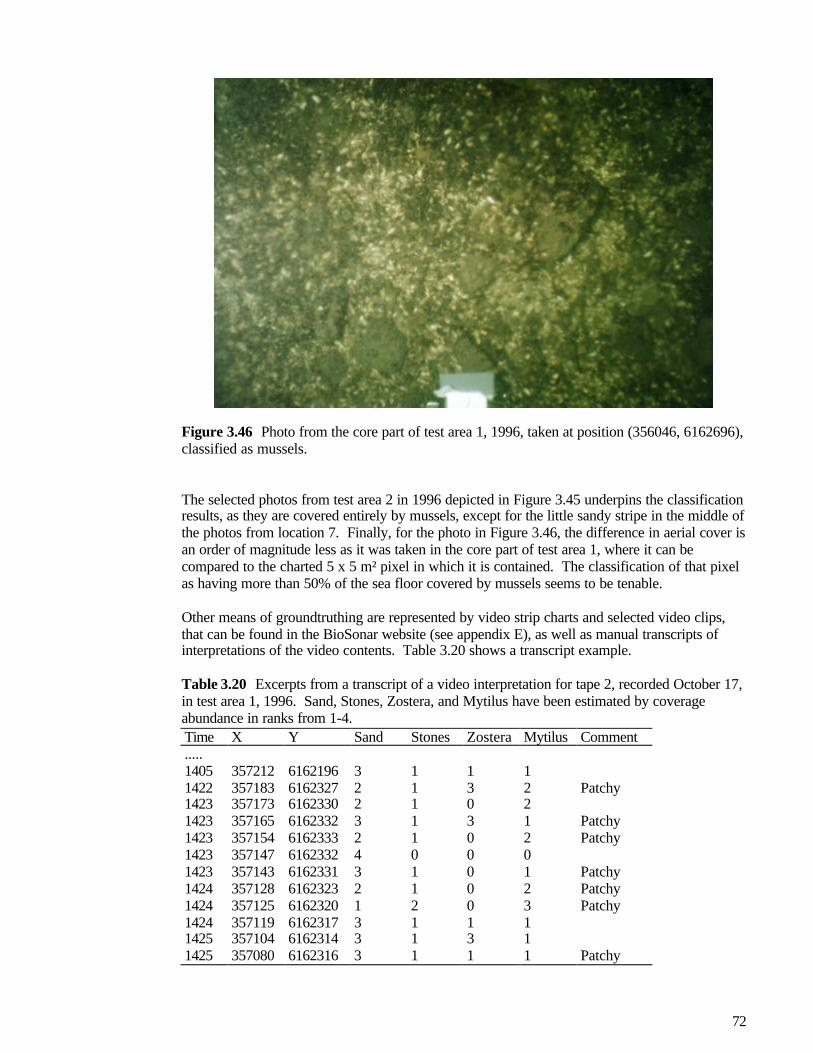
72

Figure 3.46 Photo from the core part of test area 1, 1996, taken at position (356046, 6162696),classified as mussels.

The selected photos from test area 2 in 1996 depicted in Figure 3.45 underpins the classificationresults, as they are covered entirely by mussels, except for the little sandy stripe in the middle ofthe photos from location 7. Finally, for the photo in Figure 3.46, the difference in aerial cover isan order of magnitude less as it was taken in the core part of test area 1, where it can becompared to the charted 5 x 5 m² pixel in which it is contained. The classification of that pixelas having more than 50% of the sea floor covered by mussels seems to be tenable.

Other means of groundtruthing are represented by video strip charts and selected video clips,that can be found in the BioSonar website (see appendix E), as well as manual transcripts ofinterpretations of the video contents. Table 3.20 shows a transcript example.

Table 3.20 Excerpts from a transcript of a video interpretation for tape 2, recorded October 17,in test area 1, 1996. Sand, Stones, Zostera, and Mytilus have been estimated by coverageabundance in ranks from 1-4.Time X Y Sand Stones Zostera Mytilus Comment..... 1405 357212 6162196 3 1 1 1 1422 357183 6162327 2 1 3 2 Patchy1423 357173 6162330 2 1 0 2 1423 357165 6162332 3 1 3 1 Patchy1423 357154 6162333 2 1 0 2 Patchy1423 357147 6162332 4 0 0 0 1423 357143 6162331 3 1 0 1 Patchy1424 357128 6162323 2 1 0 2 Patchy1424 357125 6162320 1 2 0 3 Patchy1424 357119 6162317 3 1 1 1 1425 357104 6162314 3 1 3 1 1425 357080 6162316 3 1 1 1 Patchy

73

Transcripts like that shown in Table 3.20 are very useful in the establishing phase of themonitoring and the development of the methodology. They do not lend themselves easily toautomation and/or quantification, wherefore the transcripts has the qualification that allinterpretation is based on qualitative estimates made once by an operator for the purpose of aquick estimation only; multiple runs made by different operators may give quite differentresults.

To shed some light on the appropriateness of the proposed mapping procedure a smallvalidation exercise was conducted in the style of Isaaks & Srivastava (1989). A vertical transectcentered on an UTM Easting of 356015 was selected, and the data in the 30 x 30 m² pixelscentered on this transect were compare to the results of the hybrid block kriging. For every 30 x30 m² pixel all observations Y = (logE1, logE2)' were classified using the classification rulesstipulated earlier, and the marginal proportions of mussels and sand in the observation sets werecalculated. These observation based proportions were compared to the proportions obtainedfrom kriging and classification of the 4 x 4 block discretisation points.

The results are depicted in Figure 3.47 and 3.48. In Figure 3.47 it is indicated that the krigingprocedure tends to yield more polarised estimates than is indicated by the observations. For the1997 datasets this is a valid interpretation of the results as the data density is approx. 48observations / pixel being markedly greater than the 16 point values / pixel used in the mappingprocedure. The upper left rectangles in Figure 3.47 indicates some deviation in the proportionestimates leading to differences in the classification results, which amounts to 7 / 48 = 14.6%for the 1997 dataset, and 6 / 47 = 12.8% for the 1996 dataset.

This tendency of the hybrid block kriged proportion estimates to be heavier tailed than theobservation based proportion estimates is clearly visible in Figure 3.48 too. As long as thepixels contain a greater amount of data locations than discretisation points, the coarseness of thediscretisation can be expected to drive the polarisation of the kriged estimates. Increasing theresolution by adding more discretisation points will not remove the polarisation, unless a scaleis reached that reflects the scale of the spatial variability. This is analogous to the polarisationeffect of using a winner-take-all voting system in democracies compared to the substantiallysmaller bias introduced by proportional representation voting systems.

Although there is some bias present, the results of this one-transect validation are consideredsatisfactory as the curves nevertheless exhibit the same patterns in Figure 3.48 and hence thekriging results can be relied upon to reflect to sea floor state in most cases. The earlierobservation of mussels spreading south from 1996 to 1997 is underlined by the rise of the plotsin the left side in 1997.

74

0.00

0.50

1.00

0.00 0.50 1.00Block averages of observations

Kri

ged

blo

ck p

rop

ort

ion

s

0.00

0.50

1.00

0.00 0.50 1.00Block averages of observations

Kri

ged

blo

ck p

rop

ort

ion

s

Figure 3.47 Scatter plots for kriged block proportions versus block proportions calculated byaveraging of observations for the pixels centered on the vertical transect at UTM Eastings of356315 m. The upper plot depicts the results for 1996, the lower depicts the results for 1997.

75

0.00

0.50

1.00

0 200 400 600 800 1000 1200 1400 1600

UTM Northing (-6162000) [m]

Est

ima

ted

mu

ssel

pro

po

rtio

ns

obs. averages

kriged prop.

0.00

0.50

1.00

0 200 400 600 800 1000 1200 1400 1600UTM Northings (-6162000) [m]

Est

ima

ted

mu

ssel

pro

po

rtio

ns

obs. averageskriged prop.

Figure 3.48 Transect line series for kriged block proportions versus block proportionscalculated by averaging observations. The upper plot depicts results from 1996 and the lowerreflects the 1997 results.

76

3.6 Summary and discussionLet us recapitulate for a moment the path travelled through this chapter. In the spring of 1996the field campaigns were designed to allow for enhanced results of the distribution mappingbased on hydroacoustic measurements. The field campaigns were executed in the fall of 1996and 1997, and the datasets were preprocessed to remove artefacts arising from lacks in thenavigation data, etc.

The obtained datasets allowed the estimation over several scales of spatial continuity andpossible anisotropy hereof. Exploratory spatial data analyses and studies of the spatialcontinuity established that data are basically stationary within areas, that logarithms of theobservations in most cases yield good approximations to Gaussian distributions, and thatactually measured values and ranges of the measurements differ markedly between 1996 and1997 (details are given in appendix B). However, the structure of the spatial continuity wassimilar for the two years, and the relative positions of data in feature space were similar too.Studies of the feature spaces of data from the bottom type areas established that thehydroacoustic observations allow basic discrimination between seafloors covered with mussels,eelgrass, and sand, respectively. Thus, the data are considered reliable and the methodology isthought to be resistant to long-term instationarities emerging over years or months; it is ofcourse vulnerable to short-term instationarities causing discrepancies between measurementsmade in a bottom type area and a test area within the same sea trial.

Kriging was used to interpolate maps of logE1 and logE2, which were combined and classifiedusing the regions derived from the feature spaces of the bottom type areas. This type ofclassification using groundtruth and observations representing distinct classes is referred to assupervised classification in the pattern recognition literature. The devised methodology wasadapted to the need for clear interpretations of the maps by using block kriging to produce(block) averages over map pixels. The kriged values representing a 4x4 points discretisation ofthe blocks were classified and used to calculate marginal proportions for mussels and sand forevery block. This procedure makes better use of the information contained than forming blockaverages of logE1 and logE2 straightforwardly and classifying the single value obtained.Comparisons to results based on a transect containing data at high densities indicate that themethodology produces viable results, although tendencies towards a polarisation bias in theestimated proportions were found, i.e. estimated proportions were more frequent in the tails atapprox. 0% and 100% than the observations.

To the best of this author's knowledge, the methodology to prepare spatial distribution mapsdeveloped here is unique, as regards the use of advanced data-driven methods of geostatistics incombination with selected bottom type areas and groundtruthing data. Related approachesinclude the traditional use of RoxAnn, and the methodologies developed and presented by thesurvey companies BioSonics Inc. and Quester Tangent Corp.

In the traditional use of RoxAnn (Chivers, Emerson & Burns, 1990; Chivers & Burns, 1991)users can interpret results in feature space (E1, E2) by use of a fixed classification map providedby the manufacturer Marine Microsystems Ltd. In many cases this can be expected to lead togross misclassification rates as the fixed division of feature space using disjoint rectangles isrigid and insensitive to behaviour of actual observations, not to mention the inexorableproblems encountered if the instationarities found in the BioSonar field campaigns are awidespread property of the RoxAnn measurements (which they might very well be). Therefore,although the original RoxAnn methodology presented a breakthrough making large scale seabed classifications workable, several elaborations have been developed in acknowledgement ofthe shortcomings of the rigid classification procedure used in the original approach.

77

The contributions made by BioSonics Inc., Seattle, WA, lie in the development of more flexiblefeature extraction algorithms and development of the necessary hardware and software enablingthis enhanced flexibility. Thus, BioSonics has developed alternative hardware devices, like e.g.the ESP Echo Signal Processor, enabling users to store digitised echo envelopes at a (user-specified) high sampling frequency. Having the full echo signal at hand allows subsequentanalysis and feature extraction to be made on a qualified basis, rather than by use of twohardwired chips producing E1 and E2 in the RoxAnn device (Sabol & Burczinski, 1998). Thisis a promising component to include in future sea bed classification methodologies, where it islikely that adaptation of feature extraction algorithms to the domain under study as well as theobjectives of the study will be a step forward.

The contributions from Quester Tangent Corporation, Sydney, Canada, lie mainly in thedevelopment of a more fine-grained classification procedure. Thus, a hardware componentparallel to RoxAnn was developed by QT, which uses the digitised signal from an echo sounderto generate a feature vector containing 150 - 166 feature elements. These feature vectors aresubsequently compressed into 3 feature variables by use of principal components analysis, andthe 3 feature variables are then used for classification purposes (Collins & McConnaughey,1998; Collins, Gregory & Anderson, 1996). The classifications can be either unsupervised if nogroundtruth is available or supervised in the presence of training data sets (Collins &McConnaughey, 1998). Based on the experience of the present study unsupervised classificationis not recommendable, at least not for the goals pursued here.

The contributions from these two companies go hand in hand focusing on separate links in thedata processing chain. However, the end results are typically presented as maps containingclassified transects shown as appropriately coloured line segments to depict the classification.No attempts are apparently made to let the classified transect observations enter a geostatisticalframework in order to produce exhaustive thematic maps of investigated regions, and here is thelink in the data processing chain where the methodology described in this chapter enters as acontribution. The approach developed here is simple, transparent and makes good use ofgeostatistics to produce full coverage maps with clear interpretations.

Meanwhile, RoxAnn remains the most used device for sea bed classification despite the limitedresolution and precision provided, mainly because it has gained widespread use for mundanepurposes like e.g., finding coral reefs or pipelines, and detecting lobsters and schools of fish. Atpresent several of the companies mentioned are directing their research into the field of dualfrequency echo sounders as a promising way of supplying an extended set of features to the seabed classification algorithms. Alternative devices are multibeam echo sounders and side-scansonars, which are discussed briefly in chapters 8 and 9.

As regards the inner workings of the methodology developed in this chapter the followingcomments can be put forth.

The kriging results rely heavily on the estimated variogram parameters which exhibitedsubstantial degrees of uncertainty in some cases, cf. the estimation of the variograms for testarea 1 in 1997, in section 3.1.4. This uncertainty could be propagated to the kriging resultssimultaneously with the uncertainty inherent in data by embedding the kriging in a Bayesianframework by use of Markov chain Monte Carlo methods (Diggle, Tawn & Moyeed, 1998).

The hard classification values applied here might alternatively be replaced by probability fieldsdescribing the somewhat crude proportion measures derived above. Alternatively, a probabilityvector for each pixel might be obtained by transforming the vector of distances from each classcenter (normalised by the dispersion norm) into a probability assigned to the correspondingcontour ellipsoid, maybe employing some degree of thresholding at a certain quantile.Subsequently, a probability field kriging (Deutsch & Journel, 1998) could be applied andpostprocessed using a threshold value like the 40% coverage rate (i.e. pixel probability value)

78

used in the Fixed Link studies (Sørensen, 1994b; Sørensen, 1995) to produce a binarydistribution map. Another approach could be to use the reverse of linear mixture modelling,called linear unmixing (Nielsen, 1997; Settle & Drake, 1993).

Because the echo sounder data are very dense along transects and very sparse in the orthogonaldirections, the order of first conducting the block kriging (by discretisation with 4x4 points forlogE1 and logE2) and then subsequently classifying these points and forming proportions (bymarginal frequencies within classes) might be reversed. Thereby, the dense trails ofobservations could be classified within a subgrid corresponding to the aforementioned 4x4discretisation points yielding local proportion estimates based on averages of classifiedobservations. These data derived proportions could then be subjected to block kriging, probablyafter use of a logit transform ( logit(p) = log[p/(1-p)] ) on the data derived proportions to havethe input to the kriging being closer to Gaussianity.

Regarding the benthic communities in question, it is seen that the separation occurs mainlyalong the E1 axis, i.e. the ruggedness scale (this is even more apparent when eelgrass isincluded, as the eelgrass observations enter the feature space in a cluster above mussels on theE1 axis). Thus, it can be argued that the echo sounder discriminates the different textures bymeans of the dominating grain size being reflected in the ruggedness measure. The featurespace classifications are not exact, bias and variability are introduced by e.g. mussels hidingbeneath seaweeds being classified as rejects, or stone and gravel at the same grain size asmussels ( ~ 5 cm length) being classified as mussels. Furthermore, there is no evidence that thefeatures used here enable the discrimination between live and dead mussels. Although thesequalifications should be recognised when using the spatial distribution maps, the methodremains a substantial improvement for the preparation of large scale, high resolution mapping.

Regarding the size of mussel beds, the preparation of distribution maps at varying scalesadapted to the varying transect densities indicated that one of the characteristic scales of musselbeds might lie in the range of 80 - 100 metres, cf. the maps for the core part of test area 1. Thisis a reproduction of a finding from an earlier study using another and less refined methodology(Sørensen, 1995).

Finally, methods to match the support of groundtruth data to the support of hydroacousticobservations, so-called footprints, and/or to the kriging results, e.g. based on up-scaling, shouldbe a priority for future studies. A comparison of the hybrid block kriging method based on awinner-take-all block voting of the discretisation points within a pixel with a more traditionalapproach based on adjusting the variograms models to the change of support, as described indetail in Journel & Huijbregts (1978), would be interesting too.

Several benefits could be gained from a study intended to reproduce the results reported here.The drift between years could be checked, and monitoring designs could sample selectedbottom type areas twice to enable a broader assessment of the precision, i.e. repeatability andreproducibility, of the measurements. Furthermore, execution of sea trials with completenavigation data rendering the pre-smoothing of coordinates within transects obsolete, wouldremove one of the concerns about the studies reported in this thesis.

An increase of the estimated mussel distribution area in test area 1 from 1.04 km² in 1996 to1.35 km² in 1997 was observed. Whether this is attributable to random fluctuations or to anactual structural change cannot be judged on a statistical basis given the results at hand. Thechapters 5 and 6 are devoted to addressing this question by use of geostatistics and imageanalysis methods.

Before moving on to that, the next chapter gives a short description of a distribution mappingstudy based on the Mediterranean data.

79

4 Spatial distribution maps forseagrasses

This chapter describes attempts made to prepare spatial distribution maps for neptune grass(Posidonia oceanica) and Cymodocea nodosa based on the Mediterranean data.

The exposition here will be based on the 1997 echo sounder data only. For a description of the1996 datasets and attempts to use these for spatial distribution mapping the reader is referred toSchultz & Ersbøll (1998), where some inherent problems with these datasets are illustrated.

4.1 Descriptive statistics and variogramsThis section gives a brief introduction to the datasets collected in the bottom type areas at Cabode Palos in the fall of 1997 and in the test area placed in the same region, and presents theestimated semivariograms to be used in the spatial interpolation.

4.1.1 The datasets from the bottom type areas at Cabo de PalosThe monitored bottom type areas at Cabo de Palos in 1997 comprise a bottom type area withPosidonia oceanica at the sea floor, one covered by Cymodocea nodosa, and three differentsand bottom type areas, covering various water depths at 13, 16 and 23 metres, respectively.The locations of the transect observations are depicted in Figure 4.1 and 4.2.

4163200

4163400

4163600

699800 700000 700200UTM Eastings

UT

M N

ort

hin

gs

cymodoceaPosidoniaSand1

Figure 4.1 Transect grids for the bottom type areas of Cymodocea, Posidonia and sand no. 1.

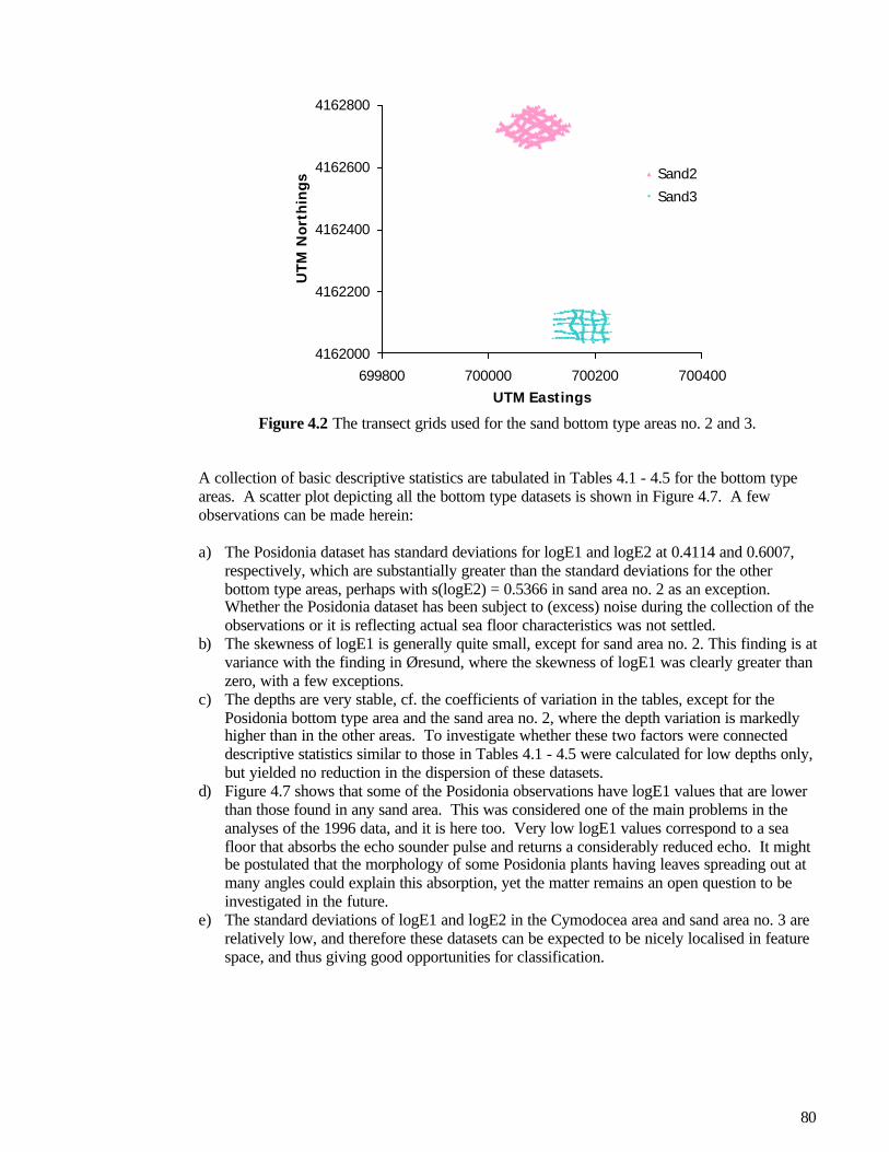
80

4162000

4162200

4162400

4162600

4162800

699800 700000 700200 700400UTM Eastings

UT

M N

ort

hin

gs Sand2

Sand3

Figure 4.2 The transect grids used for the sand bottom type areas no. 2 and 3.

A collection of basic descriptive statistics are tabulated in Tables 4.1 - 4.5 for the bottom typeareas. A scatter plot depicting all the bottom type datasets is shown in Figure 4.7. A fewobservations can be made herein:

a) The Posidonia dataset has standard deviations for logE1 and logE2 at 0.4114 and 0.6007,respectively, which are substantially greater than the standard deviations for the otherbottom type areas, perhaps with s(logE2) = 0.5366 in sand area no. 2 as an exception.Whether the Posidonia dataset has been subject to (excess) noise during the collection of theobservations or it is reflecting actual sea floor characteristics was not settled.

b) The skewness of logE1 is generally quite small, except for sand area no. 2. This finding is atvariance with the finding in Øresund, where the skewness of logE1 was clearly greater thanzero, with a few exceptions.

c) The depths are very stable, cf. the coefficients of variation in the tables, except for thePosidonia bottom type area and the sand area no. 2, where the depth variation is markedlyhigher than in the other areas. To investigate whether these two factors were connecteddescriptive statistics similar to those in Tables 4.1 - 4.5 were calculated for low depths only,but yielded no reduction in the dispersion of these datasets.

d) Figure 4.7 shows that some of the Posidonia observations have logE1 values that are lowerthan those found in any sand area. This was considered one of the main problems in theanalyses of the 1996 data, and it is here too. Very low logE1 values correspond to a seafloor that absorbs the echo sounder pulse and returns a considerably reduced echo. It mightbe postulated that the morphology of some Posidonia plants having leaves spreading out atmany angles could explain this absorption, yet the matter remains an open question to beinvestigated in the future.

e) The standard deviations of logE1 and logE2 in the Cymodocea area and sand area no. 3 arerelatively low, and therefore these datasets can be expected to be nicely localised in featurespace, and thus giving good opportunities for classification.

81

Table 4.1 Descriptive statistics for the Cymodocea bottom type area in 1997.E1 E2 Depth logE1 logE2

N 396 396 396 396 396Mean 0.2414 0.1751 12.4356 -1.4314 -1.7666

Std.dev. 0.0339 0.0394 0.3027 0.1419 0.2177Skewness 0.1435 0.7412 -0.1028 -0.1504 0.2942

CV 14.1% 22.5% 2.4% - -Range 0.164 0.211 1.8 0.7024 1.077Q3-Q1 0.055 0.060 0.4 0.2278 0.3524Max 0.325 0.320 13.4 -1.1239 -1.1394Q3 0.270 0.202 12.6 -1.3093 -1.5995

Median 0.240 0.167 12.4 -1.4271 -1.7898Q1 0.215 0.142 12.2 -1.5371 -1.9519Min 0.161 0.109 11.6 -1.8264 -2.2164

Table 4.2 Descriptive statistics for the Posidonia bottom type area in 1997.E1 E2 Depth logE1 logE2

N 311 311 311 311 311Mean 0.2165 0.0913 13.204 -1.6071 -2.5589

Std.dev. 0.0788 0.0502 1.2537 0.4114 0.6007Skewness -0.0074 0.704 -4.5139 -0.6117 -0.3419

CV 36.4% 55.0% 9.5% - -Range 0.334 0.260 15.29 1.8146 2.9741Q3-Q1 0.130 0.083 0.5 0.6211 1.0312Max 0.399 0.274 17.39 -0.9188 -1.2946Q3 0.281 0.129 13.5 -1.2694 -2.0479

Median 0.214 0.082 13.2 -1.5418 -2.5010Q1 0.151 0.046 13.0 -1.8905 -3.0791Min 0.065 0.014 2.1 -2.7334 -4.2687

Table 4.3 Descriptive statistics for the sand bottom type area no. 1 in 1997.E1 E2 Depth logE1 logE2

N 454 454 454 454 454Mean 0.1558 0.094 12.9051 -1.8709 -2.426

Std.dev. 0.0239 0.0284 0.2262 0.1511 0.3814Skewness 0.5458 -0.6415 -0.1608 0.123 -1.3586

CV 15.3% 30.2% 1.8% - -Range 0.153 0.127 1.2 0.9104 1.9129Q3-Q1 0.034 0.037 0.3 0.2202 0.3924Max 0.256 0.149 13.5 -1.3626 -1.9038Q3 0.172 0.114 13.1 -1.7603 -2.1716

Median 0.153 0.0995 12.9 -1.8773 -2.3076Q1 0.138 0.077 12.8 -1.9805 -2.5639Min 0.103 0.022 12.3 -2.273 -3.8167

82


N 345 345 345 345 344Mean 0.2963 0.0557 16.1203 -1.2371 -3.0079

Std.dev. 0.0771 0.029 1.3684 0.1858 0.5366Skewness 5.7205 0.7261 -0.7532 2.2568 -0.7148

CV 26.0% 52.1% 8.5% - -Range 0.892 0.294 6.7 2.2946 3.0706Q3-Q1 0.045 0.029 2 0.1552 0.5632Max 0.992 0.194 18.3 -0.008 -1.6399Q3 0.313 0.068 17.2 -1.1616 -2.6809

Median 0.286 0.054 16.5 -1.2518 -2.9188Q1 0.268 0.039 15.2 -1.3168 -3.2442Min 0.1 -0.1 11.6 -2.3026 -4.7105


N 387 387 387 387 387Mean 0.3958 0.1712 23.3641 -0.9323 -1.7719

Std.dev. 0.0403 0.0197 0.4314 0.1057 0.1168Skewness -0.4394 0.0594 -0.0575 -0.7679 -0.3234

CV 10.2% 11.5% 1.8% - -Range 0.24 0.122 2.8 0.6503 0.7187Q3-Q1 0.047 0.026 0.6 0.1175 0.1523Max 0.502 0.238 24.6 -0.6892 -1.4355Q3 0.424 0.184 23.7 -0.858 -1.6928

Median 0.396 0.171 23.3 -0.9263 -1.7661Q1 0.377 0.158 23.1 -0.9755 -1.8452Min 0.262 0.116 21.8 -1.3394 -2.1542

4.1.2 The dataset for the test area at Cabo de PalosA summary of descriptive statistics for this dataset is given Table 4.6. The standard deviationsfor logE1 and logE2 are at the same level as found for the Posidonia bottom type dataset, whichis not surprising as the area is large and covered with a heterogeneous blend of sea floor types.

Table 4.6 Descriptive statistics for the test area at Cabo de Palos in 1997.E1 E2 Depth logE1 logE2

N 19789 19789 19789 19789 19789Mean 0.3098 0.1447 16.402 -1.227 -2.1245

Std.dev. 0.1101 0.0954 4.5337 0.3265 0.6235Skewness 1.6471 1.6973 0.0572 0.275 -0.0602

CV 35.5% 65.9% 27.6% - -Range 1.308 0.861 23.5 2.6264 5.663Q3-Q1 0.127 0.104 8 0.4336 0.84Max 1.41 0.864 27.7 0.3436 -0.1462Q3 0.361 0.183 20.6 -1.0189 -1.6983

Median 0.287 0.117 15.2 -1.2483 -2.1456Q1 0.234 0.079 12.6 -1.4524 -2.5383Min 0.102 0.003 4.2 -2.2828 -5.8091

83

4162000

4162500

4163000

4163500

4164000

4164500

699000 699500 700000 700500 701000 701500

UTM Eastings

UT

M N

ort

hin

gs

Figure 4.3 The transect grid applied in the Cabo de Palos test area in 1997.

The transects used in the test area in 1997 are depicted in Figure 4.3, and a scatter plot of allobservations is depicted in Figure 4.4.

-3.00

-2.50

-2.00

-1.50

-1.00

-0.50

0.00

0.50

1.00

-7.00 -6.00 -5.00 -4.00 -3.00 -2.00 -1.00 0.00

logE2

log

E1

Figure 4.4 A scatter plot of logE1 versus logE2 for the Cabo de Palos test area 1 in 1997.

The contour of the scatter cloud in Figure 4.4 is shaped like a droplet much alike the shapesseen for the test areas in Øresund. It is a curiosity that the droplet shape in Figure 4.4. is tiltedby 90° compared to those found in Øresund, cf. Figure B.9, suggesting that the variables havebeen swapped. However, several checks verified that this was not the case.

84

4.1.3 SemivariogramsSemivariograms for the observed values of log E1 and log E2 in the test area were calculated byuse of the program GAMV from the GSLIB collection, version 2.0. Lag sizes of 5 metres werechosen. The SAS procedure PROC NLIN was used to estimate the coefficients of theexponential semivariogram models based on sample semivariogram data for ||h|| < 150 metres.The estimated coefficients of the variograms are given in Table 4.7, and the estimatedvariogram models are illustrated in Figures 4.5 and 4.6.

0.00

0.02

0.04

0.06

0.08

0.10

0 50 100 150 200 250 300

lag h [m]

sem

iva

rio

gra

m,

g(h

)

NESWNWSE

Figure 4.5 Sample semivariograms for NW-SE and NE-SW directions and the estimatedexponential model for log E1 in the Palos test area.

0.00

0.10

0.20

0.30

0.40

0.50

0 50 100 150 200 250 300

lag h [m]

sem

iva

rio

gra

ms,

g(h

)

NESW

NWSE

Figure 4.6 Sample semivariograms for NW-SE and NE-SW directions and the estimatedexponential model for log E2 in the Palos test area.

85

Table 4.7 Estimated parameters for exponential variogram models forlogE1 and logE2 in test area 1 in Cabo de Palos.

log E1 log E2C0 0.0102 0.0235C1 0.0606 0.1934R 121.4 100.7sill 0.0708 0.2169nugget 14.4% 10.8%

For logE1 the variogram model was estimated using the omni-directional sample variogram, asthe semivariograms in Figure 4.5 seem quite isotropic. For logE2 there is a solid zonalanisotropy for lags above 50 metres in that the sill in the direction from north-west to south-eastis clearly higher than the sill for the perpendicular direction. As the mesoscale (and microscale)contributions to the spatial continuity are important to model here, the semivariogram modelwas fitted to the sample semivariogram for the lags along the north-east to south-west orientatedtransects.

The ranges found for the variogram model, cf. Table 4.7, are remarkably high compared to theranges found in Øresund lying at values of 10 - 40 metres with one exception at 66 metres.

4.2 Feature space classificationAn introduction to classification based on discriminant analysis is given in section 3.3. Thefeature space containing observations from the five selected bottom types areas is depicted inFigure 4.7, in which it is evident that the Posidonia observations are represented as a large,diffuse cloud surrounding the population of Cymodocea measurements and the 3 scatter cloudsobtained from sand bottom type areas. Thus, they cannot be discriminated from the localisedscatter clouds of the other bottom types, and it is not considered feasible to use the Posidoniaobservations in a classification based on traditional discriminant analysis.

-3.00

-2.50

-2.00

-1.50

-1.00

-0.50

-4.50 -4.00 -3.50 -3.00 -2.50 -2.00 -1.50 -1.00

log E2

log

E1

Sand 1

Sand 2

Sand 3

Cymodocea

Posidonia

Figure 4.7 The feature space for the Mediterranean RoxAnn data from 1997 at Cabo de Palos.

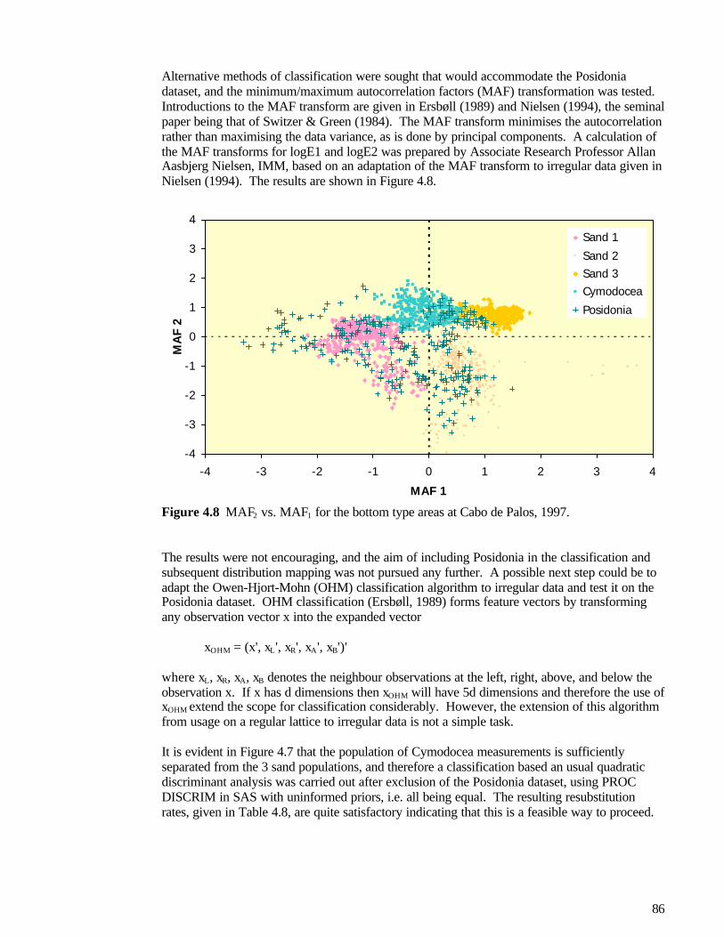
86

Alternative methods of classification were sought that would accommodate the Posidoniadataset, and the minimum/maximum autocorrelation factors (MAF) transformation was tested.Introductions to the MAF transform are given in Ersbøll (1989) and Nielsen (1994), the seminalpaper being that of Switzer & Green (1984). The MAF transform minimises the autocorrelationrather than maximising the data variance, as is done by principal components. A calculation ofthe MAF transforms for logE1 and logE2 was prepared by Associate Research Professor AllanAasbjerg Nielsen, IMM, based on an adaptation of the MAF transform to irregular data given inNielsen (1994). The results are shown in Figure 4.8.

-4

-3

-2

-1

0

1

2

3

4

-4 -3 -2 -1 0 1 2 3 4

MAF 1

MA

F 2

Sand 1

Sand 2Sand 3Cymodocea

Posidonia

Figure 4.8 MAF2 vs. MAF1 for the bottom type areas at Cabo de Palos, 1997.

The results were not encouraging, and the aim of including Posidonia in the classification andsubsequent distribution mapping was not pursued any further. A possible next step could be toadapt the Owen-Hjort-Mohn (OHM) classification algorithm to irregular data and test it on thePosidonia dataset. OHM classification (Ersbøll, 1989) forms feature vectors by transformingany observation vector x into the expanded vector

xOHM = (x', xL', xR', xA', xB')'

where xL, xR, xA, xB denotes the neighbour observations at the left, right, above, and below theobservation x. If x has d dimensions then xOHM will have 5d dimensions and therefore the use ofxOHM extend the scope for classification considerably. However, the extension of this algorithmfrom usage on a regular lattice to irregular data is not a simple task.

It is evident in Figure 4.7 that the population of Cymodocea measurements is sufficientlyseparated from the 3 sand populations, and therefore a classification based an usual quadraticdiscriminant analysis was carried out after exclusion of the Posidonia dataset, using PROCDISCRIM in SAS with uninformed priors, i.e. all being equal. The resulting resubstitutionrates, given in Table 4.8, are quite satisfactory indicating that this is a feasible way to proceed.

87

Table 4.8 Resubstitution rates for the four bottom types used in the classification. Class 1 isCymodocea, and classes 2, 3, and 4 correspond to sand areas no. 1, 2, and 3, respectively.

From CLS 1 2 3 4 Total1 381 9 0 6 396

96.2% 2.3% 0.0% 1.5% 100%2 13 424 17 0 454

2.9% 93.4% 3.7% 0.0% 100%3 13 0 331 0 344

3.8% 0.0% 96.2% 0.0% 100%4 13 0 3 371 387

3.4% 0.0% 0.8% 95.9% 100%Total 420 433 351 377 1581

Percent 26.6% 27.4% 22.2% 23.9% 100%

4.3 Spatial distribution maps for Cymodocea nodosaA spatial distribution map for Cymodocea nodosa and sand has been prepared based on ordinarypoint kriging of log E1 and log E2 in the test area followed by a classification of the pixels byentering logE1 and logE2 into the classification conducted by PROC DISCRIM in SAS. Figure4.9 depicts the resulting map comprising 2 classes, viz. sand and Cymodocea, i.e. the 3 sandclasses have been merged in the map, and Table 4.9 holds the pixel counts for the 4 classes.

699600 699800 700000 700200 700400 700600 700800 701000 701200

UTM Eastings

4162400

4162600

4162800

4163000

4163200

4163400

4163600

4163800

4164000

UTM

Nor

thin

gs

Figure 4.9 The distribution map for Cymodocea (green) and sand (yellow) prepared on thebasis of RoxAnn measurements. In grey scale yellow is lighter and green is the darker colour.

88

Table 4.9 The counts of pixels for the four populations entering the sea bed classification.

Cumulative Cumulative CLASS Frequency Percent Frequency Percent ƒƒƒƒƒƒƒƒƒƒƒƒƒƒƒƒƒƒƒƒƒƒƒƒƒƒƒƒƒƒƒƒƒƒƒƒƒƒƒƒƒƒƒƒƒƒƒƒƒƒƒ Cymodocea 5707 32.4 5707 32.4 Sand 1 1347 7.7 7054 40.1 Sand 2 8909 50.6 15963 90.7 Sand 3 1630 9.3 17593 100.0

The pixel colour counts in Table 4.9 were multiplied by the pixel size of 10 x 10 m² yielding adistribution area estimate at 0.5707 km² of the spatial distribution of Cymodocea nodosa.

Comparison with side-scan sonar based mapsThe distribution map in Figure 4.9 can be compared to the distribution map for the same areaprepared on the basis of side-scan sonar mosaics by Patricia Siljeström and Adela Moreno atIRNASE in Sevilla. This map is depicted in Figure 4.10 and contains segmentations ofPosidonia, Cymodocea and sand. It is clearly visible how the contour of the area classified as

Figure 4.10 The distribution map for Cymodocea and Posidonia at Cabo de Palos, 1997,prepared on the basis of side-scan sonar mosaics.

89

sand based on echo sounder measurements in Figure 4.9 resembles the contour of the areaclassified as Posidonia in the side-scan sonar based distribution map. This is quiteunderstandable, as the Posidonia class was excluded from the analysis of the RoxAnn data.

4.4 DiscussionThe spatial distribution map for Cymodocea can be regarded as being tentatively groundtruthedby the corresponding side-scan sonar map, thus indicating that the methodology combiningkriging and classification is feasible for Cymodocea too. This is said with the qualification thatthe discrepancy between the two maps concerning Posidonia must be resolved in other ways.

As such, the results given here and in the data report for the 1996 data (Schultz & Ersbøll, 1998)for Posidonia oceanica are not immediately encouraging. However, the lack of success heremight be overcome by similar research sea trials, and it might regardlessly stimulateelaborations of sea bed classification methods for the class of ragged textures that Posidoniaseems to be a member of. Like mussels, Cymodocea is known to have a rather smallcharacteristic scale, and therefore forms a smooth texture at the seafloor, whereas Posidoniameadows consist of large plants that can have many shapes and form a large variety of sea bedtextures. Hence, the results are perhaps not that surprising after all. Pursuance of this matter byrefining the classification algorithms is another option, either by testing the said Owen-Hjort-Mohn algorithm on these data, or by using some of the other modern classification methods likedeformable templates or neural networks.

It is this author's belief that the results for Posidonia reported here should be sought reproducedin other areas, largely repeating the designs used here too, to verify the problems encountered.Should they so prevail, other methods of detecting Posidonia oceanica can be pursued, like forexample in Bozzano et al. (1998), where the acoustic backscattering signature of Posidonia isused for detection purposes.

91

5 Geostatistical simulation of musseldistribution maps

This chapter provides a means of assessing the uncertainty of the spatial distribution maps formussels. Geostatistical simulation is used to derive estimates of coverage areas andaccompanying variance estimates. It is argued that simulated maps are valuable supplements tokriged maps of mussel distributions.

5.1 Introduction to geostatistical simulationThe need for geostatistical simulation arises when it is necessary to estimate the spatialvariability for some purpose, for example when the variability of a random field functional isrequested. An example of a random field functional is the distribution area, D, of a specific seafloor type, C, measured by the random field Z(⋅):

D[Z(⋅)] = ∫A I[Z(s) ∈ C] dA.

An exampleIn the present context, monitoring of the abundance of mussels within a larger region whereenvironmental impacts are anticipated could be an example (abundance is the biological termfor numbers obtained by counting individuals of a species). Suppose mussels have beenselected as an indicator species by an Environmental Protection Agency (EPA), and somemoderating actions are planned in case environmental impacts reach a certain level, which isexpected to be matched by a decrease in mussel abundance at 10%. The EPA would then needan assessment of the feasibility of the 10% threshold value, and - on a statistical basis - thiswould amount to whether such a decrease would be detectable in the presence of randomvariation of the mussel abundance estimate, which could be derived from mussel distributionarea estimates derived in chapter 3. Geostatistical simulation would then be needed to quantifythe variance of estimated mussel abundances.

RationaleThe interpolation procedure of kriging provides the optimum local estimates Z*(s) of therandom field over a designated grid G, i.e. Z*(s) | s ∈ G , in terms of unbiasedness, i.e.E[Z*(s)]=Z(s), and minimum mean square error, i.e. Z*(s) minimises E[(Z*(s)-Z(s))²].Therefore, the kriging estimator Z*(s) is a smoother that estimates the mean field µ(s) in Z(s) =µ(s) + e(s) and ignores e(s), maintaining the unbiasedness as E[e(s)] = 0. Hence, the univariatevariability as well as the spatial variability of Z*(s) will normally be smaller than for the randomfield Z(s) under study. This is simply a more complex manifestation of the phenomenon that amean value estimator like the arithmetic average will tend to have a variance that is less than thevariable it is averaging. Geostatistical simulation is needed to provide estimators that includethe small-scale random field e(s).

92

5.1.1 Basic theory of conditional geostatistical simulationThe following introduction is based on Journel & Huijbregts (1978) and Deutsch & Journel(1998). Geostatistical simulation aims at reproducing global properties of the spatial datasetunder investigation, primarily univariate distributions, patterns of spatial continuity andobserved values in the data locations: A) Univariate distributions are reproduced in terms offirst and second order moments as well as empirical histograms, B) patterns of spatial continuityare maintained by using models of the empirical variograms in the kriging of the simulatedvalues, and C) the data values are maintained by conditioning of the simulated values to the datapoints. Other kinds of specific global properties can be reproduced in the simulations too, butwill not be dealt with here.

A) The univariate distributions are reproduced by transforming data appropriately before use,and then back-transforming simulation results afterwards, signified by the transformationfunction ψ in Figure 5.1. In GSLIB practice (Deutsch & Journel, 1998), the transform ψ isproduced with a separate program that produces a histogram file to be used in the back-transformation too.

Z ~ F(z;θ) →ψ

U ~ Gau(0,1),U = ψ(Z)

↓

z1,..,zn,

zi = ψ-1(ui)←

ψ-1u1,.., un

(simulations of U)

Figure 5.1 Transform and back-transform applied in simulating n instances of the randomvariable Z having the (possibly empirically determined) cdf. F(z;θ).

B) The pattern of spatial continuity is maintained by calculating local conditional expectationsand variances by use of simple kriging (SK):

E[Z(s) | z(si), i=1,..,k] = ZSK*(s) = m(s) + Σi=1..k wi(z(si)-m(si))

V[Z(s) | z(si), i=1,..,k] = C(0) - Σi=1..k wiC(s-si),

where z(si) are k data values in a relevant neighbourhood of s, m(s) is the expected value of therandom variable Z(s), and the k weights wi are given by the k equations (Deutsch & Journel,1998, p. 140) in the SK system:

Σj=1..k wiC(si-sj) = C(s-si), i=1..k.

This local conditioning to maintain spatial continuity holds provided the random variables areGaussian, hence the need for the initial transformation.

C) The conditioning to data values is made by the following trick. Suppose that anunconditional simulation has been conducted yielding results zs(s) in grid nodes s ∈ G and indata locations zs(si), i=1..n, using s as a subscript to indicate simulation. Pretending the

93

simulated values zs(si) at the data locations are observed and fixed values (like the real data), thekriging of the real data is mimicked at the grid nodes to produce kriged estimates zs

*(s), s ∈ G.Having the simulated values zs(s) at hand already, the kriging error e*(s) at the grid nodes s ∈ Gcan be estimated by e*(s) = zs(s)-zs

*(s). Using an exact interpolator Z*(s) will ensure that thekriged value is equal to the observed value at data locations, i.e. z*(si) = z(si), and thereforezs

*(si) = zs(si), because the same vector of kriging weights w apply to z*(si) and zs*(si) as they

stem from identical data configurations.

Keeping in mind that the ordinary kriging estimator Z*(s) is estimating the mean field it mightbe termed µ*(s), and the conditional simulation estimator can then be expressed as

zsc(s) = µ*(s) + e*(s)

= z*(s) + (zs(s) - zs*(s)).

The conditional simulation estimator zsc(s) is thus composed of the ordinary kriging estimateproviding the mean field contribution and the simulated error estimate constructed to retain datavalues while maintaining the univariate distributions and the spatial continuity as well. Journel& Huijbregts (1978) proves that the estimator zsc(s) has the same variogram 2γ(h) as the datasetused for conditioning (in terms of the variogram model provided for the simulation), andtherefore fits its purpose.

It is required that the error estimates e*(s) and the mean field estimates µ*(s) are independent (ororthogonal), which is proved in Journel & Huijbregts (1978), p. 497. On p. 496 the authorsprove that the estimation variance of zsc(s) is twice the kriging variance, and goes on to state: "Interms of estimation variance, kriging is twice as good an estimator as conditional simulation:Estimation is not the object of simulation".

Thus, it is clear that conditional simulation cannot take the place of kriging under normalcircumstances. However, Deutsch & Journel (1998) discuss objectives that could qualify theuse of conditional simulation for estimation, and mention estimation of global features likelarge-scale heterogeneity or textures, and estimation of extreme values, i.e. tail quantiles. In thelatter case kriging is not an optimal choice as the kriging estimator is a mean squared errorminimiser targeted at local levels of the mean field, and hence suboptimal for extreme values.

Geostatistical simulation is a growing field according to Deutsch & Journel (1998), although itseems to be slightly controversial judged by the arguments given on page 4: "Recentapplications of geostatistics have de-emphasized the mapping application of kriging. Kriging isnow used to build models of uncertainty that depend on the data values in addition to the dataconfiguration. The attention has shifted from mapping to conditional simulation, also known asstochastic imaging. Conditional simulation allows drawing alternative, equally probablerealizations of the spatial distribution of the attributes(s) under study. These alternativestochastic images provide a measure of uncertainty about the unsampled values takenaltogether in space rather than one by one. In addition, these simulated images do not sufferfrom the characteristic smoothing effect of kriging."

5.1.2 The practice of conditional geostatistical simulationThe GSLIB manual (Deutsch & Journel, 1998) gives the following recipe for conductingconditional geostatistical simulations, p. 144 (Deutsch & Journel uses u for locations instead ofs, "cdf" for a cumulative distribution function, i.e. a c.d.f., and "ccdf" for a conditional c.d.f.):

"The conditional simulation of a continuous variable z(u) modeled by a Gaussian-relatedstationary RF Z(u) proceeds as follows:

94

1. Determine the univariate cdf FZ (z) representative of the entire study area and not only ofthe z sample data available. Declustering may be needed if the z data are preferentiallylocated; smoothing with extrapolation may also be needed.

2. Using the cdf FZ (z), perform the normal score transform of z data into y data with astandard normal cdf; [the program nscore from GSLIB is mentioned]

3. Check for bivariate normality of the normal score y data; […] If the multivariate Gaussianmodel cannot be retained, then consider alternative models such as a mixture of Gaussianpopulations [197] or an indicator-based algorithm for the stochastic simulation.

4. If a multivariate Gaussian RF model can be adopted for the y variable, proceed withprogram sgsim and sequential simulation, i.e.,• Define a random path that visits each node of the grid (not necessarily regular) once.

At each node u, retain a specified number of neighboring conditioning data includingboth original y data and previously simulated grid node y values.

• Use SK with the normal score variogram model to determine the parameters (mean andvariance) of the ccdf of the RF Y (u) at location u.

• Draw a simulated value y(l) (u) from that ccdf.• Add the simulated value y(l) (u) to the data set.• Proceed to the next node, and loop until all nodes are simulated

5. Backtransform the simulated normal values y(l) (u), u ∈ A into simulated values for theoriginal variable z(l)(u) = ϕ -1(y(l)( u)), u ∈ A. Within-class interpolations and tailextrapolations are usually called for; […]"

This recipe will be used in the next section to evaluate the uncertainty of the mussel distributionarea within the core part of test area 1 in 1997.

5.2 Simulation-based assessment of variabilityThe selected areaThe core part of test area 1 from 1997 was chosen to illustrate the use of geostatisticalsimulation to assess variability of distribution maps. The core part of test area 1 containstransects 20 metres apart, thus having a large data density, and it has an interesting blend ofmussels and non-mussels (rejects) at the sea floor, cf. Figure 3.34.

Figure 5.2 An illustration of classified observations in the core part of test area 1 from 1997.The darker symbols represent mussels and the lighter symbols non-mussels. The area is 120² m².

95

As in section 3.4 the core part is defined as the 120 x 120 m² area given by the UTM Eastingsand Northings [355940, 356060] x [6162680, 6162800]. The dataset from 1997 contains 2008observations herein. Using the classification function described in section 3.3 to divide allobservations into the binary classes of mussels and non-mussels, the total number of musselobservations is 1008 (~ 50.2%). The classified observations are illustrated in Figure 5.2.

5.2.1 The steps of the simulationSince the simulations in GSLIB are performed on standardised Gaussian data, a first preparatorystep is to transform the variables in question, logE1 and logE2, into normal deviates by use ofthe program NSCORE. The resulting transformation curves based on empirical histograms aredepicted in Figure 5.3, and a scatter plot of the resulting transformed variables is depicted inFigure 5.4.

-4

-2

0

2

4

-3 -2 -1 0

Ga

uss

ian

z-s

core

logE1

logE2

Figure 5.3 Transformation curves for logE1 and logE2 calculated by NSCORE.

-4

4

-4 4

Figure 5.4 Scatter diagram of transformed logE1 and logE2 values.

Before commencing to the geostatistical simulation using SGSIM, semivariograms wereprepared for the standardised Gaussian transforms of logE1 and logE2, cf. Figures 5.5 and 5.6.

96

0.00

0.50

1.00

1.50

0 10 20 30 40 50

NS

EW

Figure 5.5 Semivariogram for the transformed variable z(logE1),the standardised Gaussian deviate of logE1.

0.00

0.50

1.00

1.50

0 10 20 30 40 50

NS

EW

Figure 5.6 Semivariogram for the transformed variable z(logE2),the standardised Gaussian deviate of logE2.

Table 5.1 Estimated coefficients for exponential semivariogram models for thetransformed variables. As the standardised values have a sill at 1, only thenugget,C0, and the range, R, were estimated. C1 is then 1-C0.

z(logE1) z(logE2)C0 0.0984 ± 0.0404 0.1512 ± 0.0529C1 1-C0 1-C0R 10.83 ± 0.89 12.72 ± 1.23

For simplicity the values (10.8, 0.10) and (12.7, 0.15) of (R, C0) for z(logE1) and z(logE2),respectively, were used for exponential variogram models.

A simulation was conducted to produce 10 instances of the z(logE1) and z(logE2) random fieldsconditional on the transformed data on a grid with nodes 1 metre apart, i.e. containing 120 x 120nodes. Check statistics of the 10 simulations are given in Table 5.2. The deviations from theideal values 0 and 1 of average and standard deviation for a standardised variable are relativelysmall, except perhaps the averages of simulation no. 1, which might optionally be discarded asrepresenting an initial phase before stationarity is reached.

97

Table 5.2. Check statistics for the 10 conditional simulations generated.zE1 zE2simulation

no. average std.dev. average std.dev.1 -0.1274 1.0052 -0.1284 0.98862 -0.0328 0.9791 -0.0219 0.97333 -0.0041 0.9916 0.0110 1.01264 -0.0473 0.9706 -0.0301 1.00955 -0.0463 1.0115 -0.0381 1.04576 -0.0240 0.9812 -0.0128 1.03087 0.0021 0.9978 0.0097 0.98928 -0.0043 0.9834 0.0037 0.97609 0.0096 0.9848 0.0250 0.9914

10 -0.0647 0.9752 -0.0483 0.9998

The simulated 10 maps of logE1 and logE2 were classified by use of the rules outlined inchapter 3, and their class counts are summarised in Table 5.3. Subsequently, due to the verylow amount of sand pixels, these were identified with rejects in the images to yield the binarymaps depicted in Figure 5.7.

Table 5.3 Class counts and relative frequencies for the 10 simulated maps distribution maps.The average of the specific mussel coverage areas is 59.87% for the 10 simulations with astandard deviation at 1.12%. The class counts sum to 120² = 14400.

class counts specific areas /relative frequencies

simulationno. mussels sand reject mussels sand reject1 8915 3 5482 61.9% 0.02% 38.1%2 8712 0 5688 60.5% 0.00% 39.5%3 8485 1 5914 58.9% 0.01% 41.1%4 8708 0 5692 60.5% 0.00% 39.5%5 8375 0 6025 58.2% 0.00% 41.8%6 8483 0 5917 58.9% 0.00% 41.1%7 8560 1 5839 59.4% 0.01% 40.6%8 8533 2 5865 59.3% 0.01% 40.7%9 8678 2 5720 60.3% 0.01% 39.7%10 8759 1 5640 60.8% 0.01% 39.2%

The simulated images where merged into an average image, which was then thresholded at 0.5amounting to a simple majority decision among the 10 images about the value of the mergedpixel. This is the so-called MPM estimate (MPM = marginal posterior modes) introduced ine.g. Besag (1989). The MPM estimate of the distribution map is seen in the lower right cornerof Figure 5.7.

For comparison with the simulated maps a series of maps of logE1 and logE2 were kriged using1, 2, 4, and 8 metres as side lengths in the pixels. For the maps based on 2, 4 and 8 metrespixels cubic splines were used to interpolate the maps onto a 1 metre grid. The sequence 1, 2, 4,and 8 was applied to illuminate the degree of smoothing as a function of block size as well asthe amount of artefacts introduced by interference between the highly irregular data geometryand the relatively high resolution of 1 x 1 m² grid cells. The sequence of classified mapsprepared from the logE1 and logE2 maps is shown in Figure 5.8.

98

Figure 5.7 10 simulations of the mussel coverage in the core part of test area 1, 1997; musselpixels are black, rejects are white. The lower right corner depicts the coverage map derivedfrom a smoothed kriging (left) and the MPM estimate of the same map (right) derived bythresholding the average of the 10 images at 0.5.

5.2.2 Results and subsequent analysesIt is the impression of the simulated maps that they reproduce the mean field consistently withthe kriged map in the lower right corner of Figure 5.7 (left), with the addition of the simulatederrors embedding a certain amount of diffusion in the maps. The average map given by theMPM estimate in the lower right corner of Figure 5.7 (right) is more similar to the kriged mapthan the individual simulations as the error component is dampened by the averaging, yet it stillcontains many traces of small-scale diffusions, which the kriged map does not.

The small-scale variation in the MPM estimated map can be interpreted as a reflection of a realworld phenomenon rather than an estimation error, as mussel beds are known to have somedegree of patchiness when the mussel cover (specific area) is markedly lower than 100%, i.e. farfrom saturation. Some self-similarity of mussel pattern geometry within the scales of 5 cm - 5m would allow the conjecture that the diffused MPM map has a closer resemblance to the stateof nature than the kriged maps. The self-similarity assumption over a limited range of scaleswould allow the scaling of inference from mussel dimensions of 5 cm length to the map pixeldimensions of 1 m², even though the pixels might contain more than 400 mussels each. Snover& Commito (1998) describe a field study of these self-similar (fractal) patterns of Mytilus edulisin a soft-bottom system, and conclude that the mussel beds studied exhibited fractal qualitiesover a two orders of magnitude range of spatial scales, approx. 5 mm to 50 cm.

Assuming the small-scale heterogeneity is a real world phenomenon the MPM map could beused to point to verification sites by selecting sites fully surrounded by mussel pixels or rejectpixels, respectively. In these sites, there should be a high probability of finding a high coveragerespectively a low coverage of mussels within 1 x 1 m² pixels, which could be covered by thephoto sampler used in the BioSonar field campaigns.

99

It must be underlined that the MPM estimate is based on simulation and is therefore not the bestestimator, as mentioned earlier. Hence, individual pixels in highly diffused local regions cannotbe interpreted as optimal estimators of the sea floor class and therefore cannot apply forverification measures. However, for a joint interpretation of local regions, i.e. local sets ofpixels, the amount of small-scale diffusion seen is probably more realistic than the sharp edgesbetween the mussel regions and reject regions seen in the kriged map, as judged by transectvideos and photos from the groundtruthing data.

1 m, 67.6% 2 m, 69.0% 4 m, 69.6% 8 m, 71.1%Figure 5.8 Kriged distribution maps for square pixel side lengths of 1, 2, 4 and 8 metres,postprocessed by cubic splines to interpolate the maps onto 1 m² grids. The specific areas ofmussel coverage are given below the maps.

Another view to the estimation of small-scale variation can be discussed by looking at thekriged map sequence in Figure 5.8. As kriging is a mean field estimator the resolution of thekriged grid is sufficiently low as long as data values are not visible in the kriging results, as sucha visibility of data would reflect a small-scale variation intended to be smoothed to inferiority.This principle can be used to judge the feasibility of the resolutions used in the map sequence inFigure 5.8. Thus, the maps kriged to grid cells having side lengths of 1 m and 2 m containclearly visible traces of data, in particular along the intertwined double transect close to the rightedge of the area. Therefore, these maps are judged to have a resolution that is too high to allowkriging to estimate the mean field alone. The maps based on 4 metres and 8 metres could bothbe argued to reflect the mean field. The map based on 8 m pixels was compared to the MPMestimated map yielding the 2 x 2 frequency table given in Table 5.4.

Table 5.4 Two-way frequency table for the pixels in the binary maps obtained by kriging andsimulation. The specific areas are 67.6% for the MPM estimated map and 71.1% for the krigedmap.

MPM estimated mapfrequencies percentages

0 1 0 10 2934 1230 20.4% 8.5%Kriged map

based on 8 mpixels 1 1729 8507 12.0% 59.1%

The correlation coefficient of the two maps is 0.519, indicating the marked influence of thesmall-scale heterogeneity on the MPM estimated map. It should be underlined that the MPMestimated map is not a realisation of the hypothetical random field Z(⋅) describing musselproportions within 1 metre pixels as are the individual simulations. Rather, it is an intermediatemap lying between the kriging results and the individual realisations. This is confirmed by theconsistency with which the specific mussel area increases with increased degrees of smoothing.For the individual simulations, the specific areas lie around 60%, cf. Table 5.3, whereas thespecific area of the MPM estimated map, 67.6%, is markedly biased. The increasing degree ofsmoothing in the kriged map sequence in Figure 5.8 increases the specific area monotonicallyfrom 67.6% to 71.1% for the highest degree of smoothing.

100

Having the specific mussel areas increasing consistently with increased smoothing, i.e. havingsimilar effects as averaging, suggests that the population of measurements y = (logE1, logE2)'within the core part of test area 1 has its centre of gravity placed within the 95% confidenceellipsoid for mussels used in the classification. (The derivation of this ellipsoid is described insection 3.2). This would explain how the smoothing would tend to contract the bivariateenvelope onto a centroid posted inside this ellipsoid and hence the overlap of the ellipsoid andthe bivariate envelope of kriged results would increase as the degree of smoothing increases.

The scatter plot of logE2 versus logE1 for the core part of test area 1 in 1997 is depicted inFigure 5.9, where the centre of gravity - the centroid - is indicated with a cross.

-3.00

-2.00

-1.00

0.00

-3.00 -2.50 -2.00 -1.50 -1.00

logE2

log

E1

Figure 5.9 The feature space for the core part of test area 1 in 1997, i.e. logE1 vs. logE2. Theobservations within the mussel ellipsoid are indicated by the lighter (ocre) colour, and theobservations with the blue (darker) colour are the rejects. The cross indicates the average of theobservations.

The bivariate envelope depicted in Figure 5.9 verifies this explanation of the increasing specificareas, as the centroid is clearly within the mussel ellipsoid, and the rejects are posted at thefringe of (the right part of) the ellipsoid.

In Figure 5.10 the relative frequencies of fractions of mussel classifications assigned to everyindividual pixel are depicted. The bias of the MPM estimate is reflected by the slope of therelative frequencies from low proportions of mussel classifications to high proportions ofmussel classifications. That is, mussel pixels that are assigned to the reject class in 1 - 4 of thesimulations are much more frequent (by about a factor 3) than reject pixels that are assigned tothe mussel class in 1 - 4 of the simulations. Assuming that the simulations are ergodic thisproperty is a characteristic of the individual simulations too, and indeed the simulationsdepicted in Figure 5.7 indicate that there is a higher tendency to have spurious reject pixelswithin mussel areas than to have spurious mussel pixels within reject areas.

This is a textural feature that cannot be reproduced by kriging, and hence it is another argumentfor the case of simulation based estimation of maps for the present case. This textural feature isan observation that is coherent with the basic knowledge that mussels in Øresund tend to formclusters (Mussels normally cluster, but occasionally they form regularly distributed smallerpatches, e.g. in Limfjorden in the northern part of Denmark).

101

0.00

0.05

0.10

0.15

0.20

0.00 0.20 0.40 0.60 0.80 1.00proportion of mussel pixels

rela

tive

fre

qu

en

cy

Figure 5.10 The distribution of the relative number of mussel classifications within pixels inthe simulated images.

What is then the conclusion on this bias discussion, i.e. what is the best guess at the true musseldistribution area? The distribution area is a joint feature of the whole map and therefore theestimate must be based on the individual simulations. Certainly, the kriged map is a locallyoptimal estimator, but here the subsequent classification step depends on an extreme quantile,i.e. the 95% confidence ellipsoid, and therefore the smoothing provided by kriging is notoptimal for joint estimation. Higher credibility must therefore be assigned to the averagespecific area at 59.87% for the individual simulations than to the estimates based on smoothing,including the MPM map.

5.3 DiscussionOn the outset the present chapter was not intended to make the case for simulation basedestimates of maps, but rather to concentrate on the variability estimation issue. However, thepresentation given above indicates that simulated maps are valuable supplements to kriged mapsas regards mapping and visual exposition of regions in question, and as a means to ensureoptimality of values of random field functionals. Whereas kriging is the best local estimator asit is targeted on the mean field, the simulated maps are the best means of illuminating suchfeatures as texture and diffusion in local regions of a map. One does not have to choose, thetwo approaches are complementary by satisfying different objectives of description. Hence, theestimated map derived as the MPM estimate formed from an array of simulated random fields issuggested as a supplement to mussel distribution maps. Regarding the computation of randomfield functionals, like e.g. a sea floor distribution area for a specific bottom class, simulation ispreferable in terms of unbiasedness and as a means of estimating variability of functionals.

A simulation based MPM map could be used to point to good candidates for verification sites inthe studied region by pointing to regions where the local diffusion is low. These candidatescould then be selected for monitoring provided they are situated on an edge in the kriged map.

102

Figure 5.11 Alternative mussel distribution maps (mussel pixels are black, rejects are white):The simulation based MPM estimated map (left) containing smoothed traces of small-scaleheterogeneity, and the kriged mean field map (right).

There are other arguments for the use of simulated maps than the smoothing versus extremevalues schism. The data geometry is highly irregular due to the transect based monitoringdesign, thus the simulated maps might be the only realistic way of producing maps at highresolutions, i.e. close to the resolution of the transects. Furthermore, the exploratory spatial dataanalysis in appendix B indicated that logE1 is not strictly Gaussian, which is another reasonwhy kriging might perhaps not be the optimal estimator.

There are interesting pathways to study further in relation to simulated maps. For example, itwould be interesting to use the simulation approach to assess the effect of removing transectsfrom the grid on the resulting variance of the specific areas. Properly designed, such studieswould provide valuable input to future optimisation of monitoring designs for hydroacousticmeasurements. Another interesting pathway could be to study the properties of the simulatedmaps in scale-space to elucidate possible characteristic spatial scales of mussel beds. Ifsuccessful, results from such a study might be combined with a self-similarity model rangingover 2 or 3 orders of magnitude to be used in e.g. up-scaling of groundtruth data to reflect theresolution of kriged maps.

Returning to the question given in the opening of the chapter, the feasibility of a 10% decreaseof the mussel distribution area can now be evaluated for the core part of test area 1 in 1997.Making the assumption that the standard deviation at 1.12% applies to the next year too, the rateof decrease of the mussel distribution area could be estimated as

r = 1 - A1/A0,

where A0 and A1 are mussel distribution areas of the current year and the next year,respectively. The hypothesis testing should preferably be conducted in log space (Lyngby &Sørensen, 1994; Green, 1989; Roberts, 1993), and the hypothesis for testing the true decreaserate ρ against the stipulated value of 10% = r0 would then be

H0: log(1-ρ) ≥ log(1-0.1),

against H1: log(1-ρ) < log(1-0.1).

103

Underlying assumptions are

log A0 ~ Gau(µ0, σ²)

log A1 ~ Gau(µ, σ²)

where µ = µ0(1-ρ), and the σ² of the logarithms of estimated areas could be derived from theaverage and standard deviation above by using that var(logX) = log(1+CV(X)) holdsapproximately if CV(X) is not too high (i.e. clearly below 100%). Thus, we estimate

σ² = log (1 + 1.12%/59.87%) = 0.13614,

and would then reject H0 for values of Z such that

Z = (log(1-ρ) - log(1-r0))/σ < Φ(0.05) = -1.6445,

assuming that σ² is known, which yields a critical limit at ρ = 0.2805 using a traditionalsignificance level at 5%. When the true relative decrease is above 28.1% there is less than 5%probability of missing this incidence by testing against a decrease threshold at 10%. In a realapplication context further considerations would apply, including power calculations, etc., butbased on experience a setup like that given here would often be deemed feasible and practicable.

The point is that these calculations are made on a reliable basis provided by geostatisticalsimulation. Another point is that the variability estimates provided by the simulation make useof the data values, whereas the variances obtained by kriging depend solely on the geometry ofthe data locations.

There are some qualifications of the use of geostatistical simulation results; some of themrelated to possible lacks of ergodicity are discussed in Deutsch & Journel (1998). Furthermore,it is not known to this author whether it is possible to formulate results akin to central limittheorems for geostatistical simulations.

Therefore, in the next chapter we turn to a more simplistic random field model, that has nicetheoretical properties in terms of ergodicity and a framework providing central limit theoremsetc., thereby providing a better theoretical foundation for statistical inference of random fieldfunctionals.

105

6 A Markov Random Field approach todistribution maps of mussels

This chapter applies an alternative and very simple random field model for simulation ofdistribution maps, the so-called Ising model living on a discrete index set as opposed to themodels living on continuous index sets used so far. First, an introduction is given to Markovrandom fields and the Ising model, and the estimation and simulation of the Ising model isoutlined. By interpreting a rectangular region containing transect data as an image with amassive amount of missing data, an adaptation of an existing estimation method that accountsfor the missing data, called penalised maximum pseudo-likelihood, is presented. The model isestimated for the core part of test area 1 in 1997 and then used for simulation. The results, asregards texture and variability of image functionals, are compared to the results from thegeostatistical simulations.

6.1 IntroductionSo far the objectives of mapping the distribution of benthic communities and estimating theirdistribution area, as well as finding accompanying uncertainty measures, have been based onrandom field models living on a continuous index set, i.e. R² in a generic sense. However, arich variety of methods has been developed over the last two decades for random fields livingon a discrete index set (a lattice), i.e. N² in a generic sense, called Markov random fields. Thespatial continuity is defined by the dependency on the neighbourhood of the marginaldistributions over individual points, which is conceptually similar to the use in geostatistics ofspatial autocovariances for random fields living on R² to describe spatial continuity.

One of the main problems in dealing with coverage estimates based on distribution mapsprepared by means of classification (or segmentation) of processed echo sounder or side-scansonar data, is the lack of explicit information about uncertainty of the estimates. This stemsmainly from the fact that the distribution map normally constitutes one solitary observation,wherefore no replicates are present to be used for assessment of variability.

To overcome this obstacle several theoretical frameworks contribute means of combining asingle observation, i.e. a 2D map in this case, with a model to allow for estimation ofuncertainties by simulations. A range of synthetic datasets are produced by simulating themodel conditional on the observed map data, and used subsequently as synthetic replicates tocalculate variability measures. In the traditional geostatistical framework this can be done bysimulations based on the geostatistical model as illustrated in chapter 5. In this chapter themethodology known as Markov chain Monte Carlo simulation (MCMC) is illustrated as analternative approach, using the so-called Ising model as a model of the patterns of mussel pixelsin the map. One advantage of the MCMC methodology is that it is directly applicable to mapsproduced by either geostatistical processing of echo sounder data or maps produced by imageprocessing of side-scan sonar data.

106

The Ising model (or Ising field) belongs to the family of Markov Random Fields (MRF). Beingone of the simplest MRFs, the Ising model does not involve smoothing and might therefore be afeasible alternative description of mussel beds, at least as a first approximation.

The presentation in this chapter relies on Cressie (1991), Carstensen (1992), Higdon (1994),Guttorp (1995), Gilks, Richardson & Spiegelhalter (1996), Rosholm (1997), and Green (1998).

6.1.1 Markov random fieldsA Markov random field is a 2D sibling to the 1D Markov chain defined by the lack of memoryproperty, i.e. for the time series Y = (Y1,...,Yt)' to be a Markov chain it is sufficient that thevalue of Yt+1 depends on Yt, but not the Yi for i < t, that is

p(Yt+1 |Y) = p(Yt+1 |Yt).

Giving the t-axis a spatial rather than a temporal interpretation the Markov property states thatYt+1 depends on the neighbour Yt only. The following is straightforward, taking notice of thenotation used in image analysis and MRF theory having a tradition for using one index i onlyfor the image pixels, without loss of interpretability. The idea of Yt as a neighbour of Yt+1 canbe generalised a bit by defining a neighbourhood system N on the 2D lattice G:

N = ∂i | i ∈ G ,

where ∂i is such that

i ∉ ∂i,and

i ∈∂j <=> j ∈ ∂i,

whereby N defines a topology on G consisting of the neighbourhood sets ∂i. For digital imagesthe lack of memory property is stated as:

p(Xi | X-i) = p(Xi | ∂i)

i.e. the value of the ith pixel conditional on the rest of the image, X-i = X1,...Xi-1, Xi+1,...,Xn,depends on the neighbouring pixels only. This is often termed the local property of Markovrandom fields, i.e. that they (by definition) allow the probability distribution of the image X tobe specified by local pdf.'s for pixels conditioned on their neighbourhood. (The random fieldmust also satisfy a condition stating that all configurations of pixels X must have a probabilityabove zero, a technical condition that basically ensures ergodicity).

The random fields can describe Gaussian distributions for individual pixels, i.e. be GaussianMarkov random fields, and can be assigned many other distributions as well. In the sequel thesimplest possible type of random variable will be used, namely a binary variable, said to have aBernoulli distribution B(1,p), e.g. Xi is fully specified by p:

PrXi = 1 = p, PrXi = 0 = 1-p.

Their number of elements orders the neighbourhood systems and thus the neighbourhoodscontaining the smallest possible neighbourhood sets are called 1. order neighbourhoods, etc.For square pixels on a rectangular grid (as opposed to triangular and hexagonal grids) a 1. orderneighbourhood is given by the four closest pixels, one at the left, one at the right, one above,and one below the current pixel. This yields the definition of the Ising model, as it is identicalto a 1. order binary Markov random field.

107

Detailed introductions to Markov random fields are given in Guttorp (1995), Carstensen (1992)and Conradsen & Carstensen (1998), where the equivalence with Gibbs random fields isdiscussed as well as the celebrated Hammersley-Clifford theorem proving this equivalence. Fora general exposition of the theory of stochastic processes underlying MRFs, see e.g. Cox &Miller (1965).

6.1.2 Markov chain Monte CarloMarkov chain Monte Carlo (MCMC) is a very general methodology used to simulatedistributions that could otherwise not be obtained due to complexity. The complexity can stemfrom e.g. the distributions being hypervariable, that is containing a huge number of mutuallydependent variables, or from causal links and networks of high complexity in models. Gilks,Richardson & Spiegelhalter (1996) give examples of the many different statistical areas inwhich MCMC can solve hitherto computationally impracticable problems. MCMC is still anexciting new research area in 1999, cf. the words of Peter Guttorp (1995) in the preface: "...I tryto emphasize the importance of Markov chain Monte Carlo methods, which are having asprofound an impact on statistics in the nineties as did the bootstrap in the eighties."

The basic idea of MCMC can be stated as follows (Green, 1998). Given a distribution of interestπ(θ), θ ∈ Ω, a Markov chain θ1, θ2, ...., is constructed having π as its limiting distribution, andthe chain is then simulated and the realisations treated as a sample from π. The construction ofa Markov chain θt implies the definition of a transition kernel P(θt,θt+1) over Ω² whereby theprobabilities of state transitions are given for all θt and θt+1. The transition kernel P is ageneralisation of the transition matrix for discrete Markov chains.

Having produced a sample from π(θ) by MCMC, estimates can be calculated. For example, theprobability π(θ ∈ A ⊆ Ω) is estimated by #t ≤ N: θt ∈ A/N and the expectation of a functiong(θ) is estimated by 1/N⋅Σ t=1..N g(θt). Note the Bayesian flavour of the terminology, where e.g.π(θ) is a Bayesian posterior in most cases. MCMC can be used in other frameworks, but mostMCMC theory has been developed with a view to the Bayesian paradigm and therefore appliesnaturally in a Bayesian setting.

MCMC can be used even where static simulation cannot, as all simulation methods rely on thelaw of large numbers, which remains true due to the ergodic theorem when Markov chains areused instead of an i.i.d. sequence (i.i.d. = independent identically distributed).

To be applicable for MCMC a Markov chain must be ergodic, that is it must be aperiodic andirreducible . Irreducibility ensures that the Markov chain will not get trapped in a subspace of Ω,and aperiodicity allows any point in Ω to be reached in the next step of the chain with aprobability higher than zero (regardless of how small it might actually be). The ergodicproperties are needed for the basic MCMC limit theorems, which state that (Green, 1998):

1) If θt is an irreducible Markov chain with transition kernel P and invariant or limitingdistribution π, and g is a real valued function with ∫|g(θ)|π(dθ) < ∞, then

1/N Σ t=1..N g(θt) → ∫g(θ)π(dθ).

for π-almost all θ0.

108

2) If the chain is also aperiodic, i.e. fully ergodic, there is a stronger result implyingconvergence in distribution as well, that is

||P t(θ0,⋅) - π(⋅)|| → 0

as t → ∞, for π-almost all θ0.

MCMC is relevant to image processing, where for example the neighbourhood dependencydescribed for MRFs allow transition kernels P to be defined as local transitions making itstraightforward to construct Markov chains that simulate images. As will be shown later,MCMC can play a special role in the estimation of image models under presence of missingdata. Furthermore, the basic limit theorems of MCMC ensure that functionals derived from theMCMC simulated images are themselves stable in the sense of having a limiting distribution,and thus the MCMC framework ensures the existence of first-order and second-order statisticsfor derived image functionals as well.

Thus, whereas the image model used in this chapter might be too parsimonious, its embeddingin an MCMC framework guarantees some mathematically sound and defendable results on theother hand.

Peter Green discusses some strengths and weaknesses of MCMC in his presentation (Green,1998), mentioning the following strengths:

♦ MCMC gives a large freedom in modelling being, in principle, unlimited and because it iswell adapted for models defined on sparse graphs.

♦ MCMC gives freedom in inference as well, giving opportunities for simultaneous inferenceand allowing one to address questions posed after simulations are completed, like e.g.ranking and model selection.

♦ It is the only available method for complex problems.♦ MCMC integrates uncertainty coherently and allows for model comparisons, -criticism, and

-choice and also encourages sensitivity analysis.

He is also listing the following weaknesses and dangers:

♦ MCMC implies the risk that fitting technology runs ahead of statistical science.♦ There are difficulties in validating computer code.♦ There are risks of MCMC leading to undisciplined, selective presentations.♦ Possibilities of slow convergence that might not be diagnosable.

Good introductions to MCMC can be found in Gilks, Richardson and Spiegelhalter (1996), andin Guttorp (1995), and a good overview of the application of MCMC with four detailedexamples is given in Besag et al. (1996).

6.2 The Ising modelThis section introduces the Ising model and some of its characteristics, followed by outlines ofhow to simulate and estimate Ising models.

6.2.1 Basic properties of the Ising modelThe Ising model originated within statistical mechanics as a model to describe magnetisation. Atwo-dimensional grid or lattice is supposed to contain one of two values in every cell (originally

109

positive or negative magnetic spin) and the cells are assumed to be correlated to their nearestneighbours adjacent to the four cell edges. (The rectangular grid based on squares is just one ofseveral basic grids, other grid types like the hexagonal can be applied). The value of the ith

pixel, Xi , is thus influenced by the neighbours j ∈ ∂i, a relation that defines the local conditionalprobabilities

p(Xi = xi | ∂i) = exp(xi⋅[α +β1(xw+xe) +β2(xn+xs)]) /(1+exp(α +β1(xw+xe) +β2(xn+xs))),

where the members of ∂i = xw, xe, xn, xs are the neighbours of xi at the west, the east, the northand the south. In this parameterisation, which is common in image processing, β1 controls thenumber of horizontal 1-1 neighbours and β2 controls the number of vertical 1-1 neighbours.This interpretation is valid under the assumption that the set 0,1 was used for the binarycoding of pixels. When β1 = β2 = β the Ising model is said to be isotropic . The parameter αcontrols the amount of 1-pixels, assuring a mean fraction at 0.5 when α = -(β1+β2). If the meanfraction of 1-pixels is 0.5, the Ising model is said to be symmetric or having a zero field .Denoting the local conditional probability of Xi being a 1-pixel by p, we write

p = p(Xi = 1 | ∂i) = exp(α +β1(xw+xe) +β2(xn+xs)) /(1+exp(α +β1(xw+xe) +β2(xn+xs))),

and hence

logit p = log(p/(1-p)) = α +β1(xw+xe) +β2(xn+xs),

which can be averaged over all 16 combinations of pixel values for the neighbours to yield

logit p = log(p/(1-p)) = α +β1 +β2,

from which it is evident that we can set p equal to 0.5 locally and obtain α = -(β1+β2) as thecondition for symmetry. It is my conjecture that the relation

log OR(µ) = logit µ = <θ,1> = α +β1 +β2 (6.1)

where µ is the global mean fraction of 1-pixels, i.e. the image mean value, and θ is theparameter vector (α, β1, β2)', holds too, but it has not been within my reach to consult therelevant papers, e.g. Martin-Löf (1973), which might contain the relevant proof. The symbolOR indicates that the figure is the odds ratio of the mean, known from logistic regression(Kleinbaum, 1994). In some contexts the Ising model is described as a spatial logistic model(Cressie, 1991). Log odds ratios will be used as indirect measures of the external fields, i.e. themean fractions, in the following sections.

If (6.1) holds globally, it can be used to compute the mean fraction, µ, when the parametervector θ = (α, β1, β2)' is known or estimated.

The joint probability of an image X = X1, ..., Xn for the isotropic model is

P(X = x) = 1/c(α,β) ⋅ exp(αΣixi) exp(βΣiΣ j∈∂ixixj) (6.2)

where c(α,β) is a normalisation constant, sometimes referred to as the partition function(Carstensen, 1992; Guttorp, 1995).

The original parameterisation assumed that pixels be coded from the set -1,1 of spins. In thatcase the interaction parameters, β1 and β2, control the number of identical neighbours in eitherdirection, and α controls the mean fraction.

110

The parameterisation of the isotropic Ising model can be generalised to read (Higdon, 1994)

P(X = x) = 1/c(α,β) ⋅ exp(αΣixi) exp(β Σ iΣj∈∂i I[xi=xj]) (6.3)

allowing α to control the mean fraction, µ, as α = logit µ, and letting the β coefficient controladjacencies of identical pixels, regardless of the coding of the pixels. Both parameterisationsare used in this chapter. The first given by (6.2) will be referred to as the Carstensen-parameterisation and the second given in (6.3) will be referred to as the Higdon-parameterisation. When not explicitly stated, the Carstensen-parameterisation is assumed. Inthe Higdon-parameterisation α is called the external field, and the β's are called interactionparameters (as mentioned above).

The Ising model got its name from the original work in 1923 by the graduate student Ising, whoshowed that the 1-dimensional model had no phase transition, i.e. the magnetization variedcontinuously. The other main contributor is Onsager (1944) who gave the exact solution to the2-dimensional problem in 1944, showing that it had a phase transition of the type seen in realferromagnets. This led to great advances in the theory of phase transitions and criticalphenomena.

The phase transition is illustrated in the example images in Figure 6.1 simulated for a symmetricand isotropic Ising model. For β = 0 a binary white-noise image is obtained, and for β at 0.5,1.0, 1.5 and 1.7 it is seen that the size of clusters containing identical pixels increase whileretaining the symmetry, i.e. having about an equal number of 1-pixels and 0-pixels in theimages. When the β coefficient approaches the percolation limit of 2⋅sinh-1(1) ≈ 1.7627 (halfthis value, ≈ 0.88, for the Higdon-parameterisation), percolation begins to emerge, i.e. pixels ofthe same colour begin to form very large clusters that tend to have a global outreach. For βabove 1.7627 it is seen that the image is covered almost solely by one of the two kinds of pixels,leaving just a few speckles of the other pixel type in the images. In the phase transition themean fraction of a symmetric joint distribution is still 0.5, but the mean is now divided image-wise instead of pixel-wise locally in the images. This is graphed in Figure 6.2, showing thebifurcation of the mean fraction in a sample image, i.e. a realisation from the joint distribution.

Onsager (1944) showed that the phase transitions occur for values above the so-called criticalitylimit and that this limit is defined for the anisotropic model by the equation

crit(β1,β2) = sinh(β1/2)sinh(β2/2) = 1. (6.4)

Coefficients β1 and β2 for which crit(β1, β2) > 1 are said to be supercritical, whereas thosecorresponding to crit(β1 , β2) < 1 are said to be subcritical. The state of supercriticality or phasetransition is also referred to as long-range correlation, as it can be shown that any image pixel iscorrelated to the border pixels when the coefficients are supercritical, independently of the sizeof the image.

There are many similarities to random fields with continuous support. The external fielddescribed by α is stationary for α being a single, global variable (using the Higdon-parameterisation here). It is straightforward to introduce an external field by specifying αlocally, i.e. α is replaced by the matrix A = αi describing the external field at every site.This is similar to geostatistical applications where kriging of a stationary field can beaugmented by an external field, which is presumably described by some smooth function; insimple cases a quadratic polynomial will suffice. The same idea could be used to fill in A witha smooth external field. A more stochastic approach would be to use an underlying data imageas a prior thereby letting αi depend on yi in the data image without fixing the site value xi in theestimated image, i.e. αi < ∞. Higdon (1994) contains several examples of applications of theseideas.

111

β = 0 β = 0.5 β = 1.0

β = 1.5 β = 1.7 β = 1.76

β = 1.8 β = 2.0 β = 3.0

Figure 6.1 Example configurations for the symmetric isotropic Ising model for an increasingsequence of β values.

0.00

0.50

1.00

1.0 1.5 2.0 2.5 3.0-5

-4

-3

-2

-1

0

1

2

3

4

5

-5 -4 -3 -2 -1 0 1 2 3 4 5

Figure 6.2 Illustrations of the phase transition in the Ising model. At the left, the meanfraction, µ, of 1-pixels is depicted for the symmetric isotropic Ising model as a function of β.The phase transition occurs at β = 2sinh-1(1) = 1.762747. At the right, the phase transitionboundaries given by (6.4) are depicted for the anisotropic model.

112

The Ising model is aperiodic and irreducible, hence an ergodic theorem applies and it can beused in an MCMC framework. Applications of the Ising model and binary MRFs in imageanalysis comprise image restoration, texture simulation, etc. For more details about MRFs andtheir use in image modelling the reader is referred to Carstensen (1992) and Higdon (1994).

6.2.2 Simulation of the Ising modelThe early methods of simulating Ising models relied on single site updates like Metropolissampling (Hastings, 1970) and Gibbs sampling (Geman & Geman, 1984). These algorithmsvisit every individual pixel and use smart ways of expressing the local conditional probability,i.e. (6.1) or (6.2), with regard to simulation purposes. This has evolved into a subfield of itsown within the MCMC framework, where updating and mixing algorithms are studied in theframework of the Metropolis-Hastings-Green (MHG) update mechanisms (Geyer, 1998) for usein other types of models.

For Ising models the single-site updates were succeeded by the cluster updating methods, nowknown under the name of auxiliary variable methods. The first and seminal algorithm was theSwendsen-Wang cluster update (Swendsen & Wang, 1987), which has formed the basis for avariety of elaborations. Being one of these, the partial decoupling algorithm was introduced byHigdon (1994) and works like a very user-friendly version of the Swendsen-Wang algorithm. Ashort sketch of the Swendsen-Wang and the partial decoupling algorithms is given in thefollowing.

The Swendsen-Wang algorithm (SW) is sketched in Table 6.1. An auxiliary "bond" variable, u,is used to form bonds between sites, i.e. uij = 1 means that xi and xj are connected, while uij = 0means that they are not. The rationale is that by specifying bonds by the variable u it is possibleto decouple the interaction terms from the external field term. We define π(u|x) to let the uij's beindependent and uniformly distributed. The interaction coefficients enter the realisations of theu variable by controlling the probability of bonding, i.e.

p(uij=1| x) = 1-exp(-βij)

where βij = β1 for horizontal neighbours and vice versa. Subsequently, the bonds can betraversed to form clusters of bonded pixels and the clusters can then be assigned a value usingthe external field only, i.e. with a probability proportional to exp(αΣ i∈C xi ) over the cluster C.In other words, when each cluster has been assigned a colour the sweeping step is done. Thisprocedure gave a tremendous speed up of computation time, in particular for larger images.

Table 6.1 Swendsen-Wang algorithm (SW).

for every sweep of the image: given x, update u:

setup bonds between sites using β1 and β2

label clusters and assign cluster IDs to sites given u, update x:

assign colours to clusters using αassign cluster colour to all sites

The SW algorithm speeds up computations by a high rate. However, some deficiencies arisewhen e.g. the SW algorithm is used with an external field and strong interactions, i.e. havingthe mean fraction µ differing from 0.5, or when SW is sought used for sophisticated simulationpurposes like simulating images conditional on partial data. If some of the pixels of the imageare fixed, as they would be when simulating conditional on data, the SW algorithm may move

113

slowly through the sample space, when a majority of the clusters contain data and thereforehave a zero probability of changing colour. Elaborations of the Swendsen-Wang that allowedfor conditional simulation and good mixing when used with external fields were sought andHigdon (1994) suggested the partial decoupling algorithm as a generalisation of the Swendsen-Wang that can be adapted easily to a range of application purposes.

Table 6.2 Partial decoupling algorithm.

Setup decoupling weights λij

for every sweep of the image: given x, update u:

setup bonds between sites using β1 and β2

label clusters and assign cluster IDs to sites given u, update x:

determine cluster bordersassign colours to clusters using α, β1 and β2

assign cluster colour to all sites

The partial decoupling algorithm is sketched in Table 6.2. A user-specified matrix containingthe decoupling weights λij as fixed constants is used to direct the simulations. The decouplingweights enter the simulations the expression of the bonding probabilities for uij now read

p(uij=1| x) = 1-exp(-λijβij)

and the price for introducing these weights is that the clusters are no longer independent of oneanother, conditional on the bond variables, u. Hence, it is necessary to update clustersconditionally on their neighbours. The theoretical details of the conditional probabilitiesinvolved are given in Higdon (1994). That partial decoupling is a generalisation of the SWalgorithm is easily seen as it is identical to Gibbs sampling when all λij = 0 and identical to theSW algorithm when all λij = 1.

Partial decoupling is easily used for simulations conditional on data. Setting λij = 0 for j ∈ ∂ifor all data pixels xi and setting all other λij = 1 will prevent any neighbouring pixel frombonding with the data pixel while using the SW updates away from the data pixels.

In the simulations prepared here, a guard region at 10% width was added to the images and thena so-called periodic boundary was used, meaning that the image is simulated on a torus, lettingleftmost and rightmost pixels in a row be neighbours, as well as topmost and bottommostneighbours.

6.2.3 Maximum likelihood estimation for the Ising modelThe full likelihood for the Ising model is not computable in practice, hence the traditionalsolution to parameter estimation prescribes to maximise the so-called pseudo-likelihood instead(Cressie, 1991; Carstensen, 1992). The pseudo-likelihood is given by assuming that pixels areindependent, wherefore the expression

PL = Π pixi (1-pi)1-xi

can be maximised leading to the maximum pseudo-likelihood (MPL) estimate. In practice thelogarithm of PL is maximised, i.e. the function f(θ) is used:

114

f(θ) = log PL = Σi [xiTi - log(1+exp(Ti))], (6.5)

where θ = (α, β1, β2)', si = (1, xw+xe, xn+xs)', Ti = θ'si, and pi = exp(Ti)/(1+exp(Ti)).

Feeding f(θ) and the gradient

∇f(θ) = Σ i [xi-pi]si (6.6)

and Hessian matrix

∇²f(θ) = -Σ i pi/(1+exp(Ti))⋅sisi' (6.7)

to a computerised maximisation routine (like e.g. NLPQN in SAS/IML) an estimate of θ can beobtained. It is not straightforward to derive an initial starting guess θ0 = (α0, β10, β20)' from thesufficient statistics of the image (t0, t1, t2)', where

t0 = 1/N Σixi, (6.8)

t1 = 1/N ΣiΣ j∈∂i xixj for horizontal neighbours, and

t2 = 1/N ΣiΣ j∈∂i xixj for vertical neighbours,

however, the relation

α0 +β10 + β20 = logit t0, (6.9)

can be combined with reasonable isotropic initial values for β in the range of 1.0 - 1.5 with goodresults because the MPL algorithm is rather robust as regards avoiding falling into local maxima(Carstensen, 1992).

Other methods apply, e.g. Besag's coding set method (Besag, 1974), but the MPL method hasgained widespread use due to its simplicity and its ability to produce good estimates (Cressie,1991; Carstensen, 1992).

6.3 Ising model estimation for images with missing dataThe MPL estimation outlined in the section above is implicitly assumed to work on imageswhere all pixels are known, i.e. given by a measured value in some sense. However, thetransect data only account for a small fraction of the pixels, leaving the rest as unknowns. TheIsing model would not be estimable if the data were scattered all over the field as in traditionalgeostatistical datasets, leaving no data pixel pairs to be used in the estimation of the interactioncoefficients, β (unless a very coarse discretisation is applied to the data). The one-dimensionalnature of the transect data ensures that a feasible number of pixel pairs is present and allows theMPL estimation to be carried out. However, when the transect data are discretised and filledinto an image, the fraction of missing data pixels is still rather high, typically at least 90%.Naturally, the actual fraction of missing data for a dataset depends on the size of the pixels usedfor the discretisation of the image.

In acknowledgement of the crude accuracy (accuracy comprising bias and precision) of MPLestimates under these circumstances, the plan was to use the MPL estimate as an initial goodstarting guess for a refined and complex maximum likelihood algorithm called MCL. CharlesGeyer discusses MCL in several papers, e.g. Geyer & Thomson (1992) and Geyer (1998), and

115

Guttorp (1995) gives a good basic introduction to the MCL method as well. Geyer (1998)describes in detail how the method might be used for cases of missing data to obtain goodestimates within a MCMC framework.

It turned out that the MPL estimates tend to break down when the fraction of missing pixels liessomewhere between 80% and 90% and, moreover, vast numerical difficulties were encounteredwhen the MCL method was implemented, due to its highly non-linear properties. Thebreakdown properties of the MPL estimates were studied and lead to a penalised version of thepseudo-likelihood algorithm, by which penalised maximum pseudo-likelihood estimates(PMPL) can be obtained. This section gives the details of the studies leading to the PMPLmethod and presents the theory behind the MCL estimation procedure.

6.3.1 Maximum pseudo-likelihood for images containing missing dataPreliminary attempts to produce MPL estimates for images containing binary coverage data aswell as missing data indicated that the MPL estimates get inflated when the fraction of missingdata reaches a certain level in the interval of 80% - 90%. Thus an experiment was conducted tostudy the properties of this breakdown using sequences of images derived from an initial fullimage by removing an increasing fraction of the pixels, i.e. assigning them to the class ofmissing values. The removal of pixels was done by removing an identical number of columnsand rows leaving equidistant rows and columns of data pixels in the image, thereby producing asequence of increasingly thinned images, cf. Figure 6.4.

In the thinning experiment described in the sequel the fraction of missing data is used as thecritical measure for the breakdown of the MPL estimation. The most accurate measure to usewould be the number of missing pixel pairs, as this is the critical number for the estimation ofthe interaction coefficients. However, as this fraction is considered to be proportional to thefraction of missing pixels due to the strict one-dimensional geometry of the transect data, thelatter is used in the sequel.

The image thinning experimentIn order to emulate the properties of an image given by classified transect data containing amajor amount of missing data, i.e. void pixel values, an image thinning experiment was carriedout. A set of 7 images containing 128 x 128 pixels were simulated to closely mimic the area tobe studied, i.e. the core part of test area 1 being 120 x 120 m². A symmetric Ising field wasassumed with isotropic β values at 1.5, which are values anticipated to be close to the endresults, i.e. the parameter vector θ = (-3.0, 1.5, 1.5)' = (α, β1, β2)' was used. An interactioncoefficient, β, at 1.5 ensures that clusters (mussel patches) can be contained by the model whilemaintaining a local nature of the clusters, as an isotropic β = 1.5 is subcritical. The 7 simulatedimages are depicted in Figure 6.3.

For every image a sequence of increasing thinning was generated by retaining the values inevery kth row and column for k = 4, 8, 10, 12, 14, 16, 18, and 20 corresponding to fractions ofmissing pixels at 0.562, 0.766, 0.821, 0.850, 0.864, 0.879, 0.894, and 0.908. One of theresulting image sequences are illustrated in Figure 6.4 for the first image (a) in Figure 6.3, andbear good resemblance to the geometry of the real world transect data.

The image sequences were fed to a maximisation routine (NLPQN in SAS/IML) to obtain MPLestimates θ* of θ = (α, β1, β2)' for k = 4, 8, and 16 initially, to be checked for recovery of thetrue values of θ = (-3.0, 1.5, 1.5)', cf. Figure 6.5 and Figure 6.6. Figure 6.5 depicts inflationmeasured by ||(β1,β2)'||/||(1.5,1.5)'|| and the relative criticality crit(β1 ,β2)/crit(1.5,1.5), where β1

and β2 are estimated values. Figures 6.5 and 6.6 show that instabilities occur at k = 16, i.e. at afraction of missing data at 0.879.

116

(a) (b) (c) (d)

(e) (f) (g)Figure 6.3 The 7 simulated images employed as a basis for the thinning experiment.

image (a) 4 8

10 12 14

16 18 20Figure 6.4 The image thinning sequence for image (a) in Figure 6.3, retaining every kth rowand column for k = 4, 8, 10, 12, 14, 16, 18, 20. Grey pixels indicate missing values.

117

0.00

0.50

1.00

1.50

2.00

2.50

0.00 0.20 0.40 0.60 0.80 1.00

Fraction of missing data

Inflation

rel. criticality

Figure 6.5 Inflation and relative criticality for the interaction coefficients, β1 and β2, forthinned images given by k = 4, 8, and 16. The inflation is measured as the length of (β1,β2)relative to the true vector (1.5,1.5), i.e. by ||(β1,β2)'||/||(1.5,1.5)'||, where β1 and β2 are estimatedvalues. The relative criticality is measured by crit(β1,β2)/crit(1.5,1.5). The markers indicateresults for individual image sequences and the lines indicate the averages of the measures.

-1

0

1

2

3

0 1 2 3 4-1

0

1

2

3

0 1 2 3 4

Figure 6.6 Trajectories of (β1,β2) estimates for increased thinning rates in the β phase space,showing a clear inflation at the high end of the interval of thinning rates. At the right thetrajectories are depicted with error bars indicating the standard deviations of the β's derivedfrom the Hessian matrix. Abscissas and ordinates are β1 and β2, respectively.

Subsequently to the initial experiment, extra thinnings k = 10, 12, 14, 18, and 20 were added tothe image sequences as an effort to locate the limiting fraction of missing data pixels abovewhich the inflation occurs in the interval between 80% and 90%. The biases found in the MPLestimates for criticality, mean fraction and anisotropy for the extended image sequences aredepicted in Figures 6.7 - 6.9, which depict the odds ratios, the relative criticalities, and theanisotropy biases, respectively. The latter is given as max(|β1/β2|, |β2/β1|).

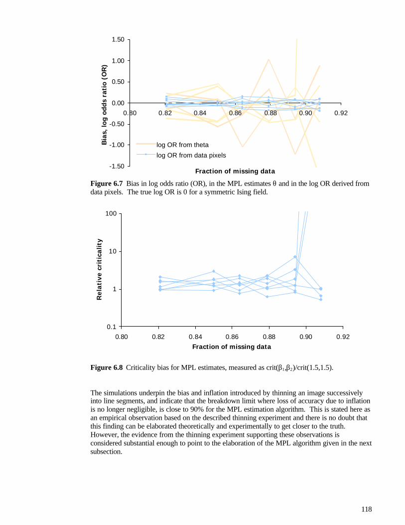
118

-1.50

-1.00

-0.50

0.00

0.50

1.00

1.50

0.80 0.82 0.84 0.86 0.88 0.90 0.92


Bia

s, lo

g o

dd

s ra

tio

(O

R)

log OR from theta

log OR from data pixels

Figure 6.7 Bias in log odds ratio (OR), in the MPL estimates θ and in the log OR derived fromdata pixels. The true log OR is 0 for a symmetric Ising field.

0.1

1

10

100

0.80 0.82 0.84 0.86 0.88 0.90 0.92Fraction of missing data

Re

lati

ve c

riti

cali

ty

Figure 6.8 Criticality bias for MPL estimates, measured as crit(β1,β2)/crit(1.5,1.5).

The simulations underpin the bias and inflation introduced by thinning an image successivelyinto line segments, and indicate that the breakdown limit where loss of accuracy due to inflationis no longer negligible, is close to 90% for the MPL estimation algorithm. This is stated here asan empirical observation based on the described thinning experiment and there is no doubt thatthis finding can be elaborated theoretically and experimentally to get closer to the truth.However, the evidence from the thinning experiment supporting these observations isconsidered substantial enough to point to the elaboration of the MPL algorithm given in the nextsubsection.

119

0

1

2

3

4

5

0.80 0.82 0.84 0.86 0.88 0.90 0.92


An

iso

tro

py

bia

s

Figure 6.9 Anisotropy bias for MPL estimates measured by max(|β1/β2|, |β2/β1|).

The development of bias as a function of the amount of missing data in the log odds ratio, logOR(θ), given by (6.1) is displayed in Figure 6.7, which also indicates that the log OR derivedfrom the data still left in the image is more stable than the estimated log OR. Thus, the imagestatistic for the OR can be used to provide a good initial value θ0 and to penalise largefluctuations in the OR(θ). Thus, the next subject is introduced as it is evidently required torepair the MPL algorithm for the inflation and related loss of accuracy encountered when thefraction of missing pixels is high, i.e. above 80% - 90%. These high fractions apply to thedataset to be studied from test area 1.

What is needed is a way of supporting the estimation by imposing certain regularity measures,such that the optimality of θ will depend on the pseudo-likelihood and on the regularity criteriaas well. Adding such regularity criteria to an estimation procedure is known as penalisation, i.e.the secondary criterion is specified as a penalty on the object function of the maximisation. Thesetup of a penalty vector and a comparison of the penalised MPL with the ordinary MPL isdescribed in the next section.

6.3.2 Penalised maximum pseudo-likelihoodIn some frameworks the following elaborations are termed regularisation (Nielsen, 1998).However, it is preferred to reserve the word 'regularisation' for cases of massively multivariateestimation problems, where some smoothness condition, normally expressed as a penalty onfirst- or second-order derivatives, is applied in the elementary approaches (Green, 1998a). Herewe deal with an estimation vector θ containing three elements and the general term 'penalisedlikelihood' will apply. In usual maximum likelihood θ is estimated as the argument value wherea maximum of the likelihood function L(θ) is found, i.e.

θML = arg max [L(θ)],

whereas in penalised maximum likelihood a penalty criterion P(θ) is added to obtain thepenalised maximum likelihood estimate θ by:

θPML = arg max [L(θ) - λP(θ)]

120

where λ is a multiplier either to be included in the maximisation as an auxiliary parameter or tobe assigned a fixed value before the optimisation is carried out.

A simple example of penalised likelihood is in model selection likelihood, where the penaltyadjusts the likelihood function for the number of parameters entering the model(s) by use of e.g.the Akaike information criterion, AIC, or the Bayes information criterion, BIC. Green (1998a)gives another example, describing how the optimal selection of splines for empirical curvefitting leads to selection of the well-known cubic splines when a penalty on the lack ofsmoothness of the second-order derivative is added to the minimisation of the sum of squares.

Thus, a penalty vector was applied to regularise or calibrate the estimation to the condition of amassive amount of missing data. The penalty vector,

P(θ) = (p1²(θ), p2²(θ), p3²(θ))'

is usually specified by quadratic penalty elements, making inference and derivatives easy tohandle and interpret. Some authors prefer to use a linear criterion Pi(θ) = |pi(θ)| rather than aquadratic Pi(θ) = pi²(θ), and Green (1998a) suggests a generalisation using Pi(θ) = logcosh(pi(θ)/∂), where ∂ can be used to calibrate the power of the expression in the intervalbetween 1 and 2.

Three penalty elements have been defined to penalise departures in θ regarding supercriticality,mean fraction or log odds ratio, and anisotropy.

CriticalityThe penalty for supercriticality is based on considerations of the phenomenon that is modelledwith the Ising field, i.e. it is partly based on a domain-specific argument. If the images coversufficiently large areas and the data indicate that the area is not totally covered by mussels (i.e.that the mean fraction of the data pixels is clearly less than 1), then it can be assumed thatmussel patches will exhibit a local structure and not be globally connected. Furthermore, it canbe argued that supercritical interaction coefficients are generally undesirable for mussel bedsbecause they would imply that mussel beds are bimodal in the large global areas studied. Meanfractions of mussel beds close to 1 (or 0) are thus better modelled by imposing a strong externalfield and keeping the interaction coefficients in the subcritical region.

Apart from these domain specific arguments, the thinning experiment showed that theinteraction coefficients have some tendency to inflate markedly and thus a criticality penalty isreasonable as a means to control the inflation hereof. The inflation of the interactioncoefficients could alternatively be controlled by a penalty on the Euclidean length of the vector(β1,β2). However, it was found recommendable to use the penalty for the criticality measure asit applies at a higher qualitative level due to the domain-specific arguments given above.

In operational terms it is assumed that the interaction coefficients comply with the inequality

crit(β1,β2) = sinh(β1/2) sinh(β2/2) < 1.

A straightforward penalty would be p1(θ) = crit(β1,β2), as this would assume high values forsupercritical β values. However, this criterion was found to be too weak for practical purposesand something more akin to thresholding of supercritical values was searched for, whilemaintaining simplicity of the penalty expression. Thus, to make this penalty behave like a blendof a penalty and a thresholding, a quartic penalty, i.e. a double squared penalty, was used:

p1(θ) = [crit(β1,β2)]². (6.10)

121

Mean fractionA simple linear penalty was used to control the departures from the log odds ratio, which issimply logit(t0), where t0 is the mean fraction estimated from the data pixels by use of (6.8):

p2(θ) = <θ,1> - log OR = α +β1 +β2 -logit(t0).

AnisotropyIt is not the intention to impose isotropy on the interaction coefficients with this penalty. If thatwas the case, it would be much simpler to estimate an isotropic Ising field directly. The intentis to counteract the tendency to get highly artificial anisotropic coefficients due to the inflation,which was observed in the thinning experiment. To penalise anisotropy the followingexpression was used:

p3(θ) = (β1/β2+β2/β1)/2.

The maximisation function, f(θ), the derivative and the Hessian given by (6.5), (6.6), and (6.7)are then supplemented with the penalty vector to yield the following maximisation system:

g(θ) = f(θ) - <λ,P(θ)>,

∇g(θ) = ∇f(θ) - <λ,∇P(θ)>,

∇²g(θ) = ∇²f(θ) - <λ,∇²P(θ)>,

and the penalised pseudo-maximum likelihood (PMPL) estimate θ* of θ is the argument valuewhere g(θ) is maximised.

The PMPL method has the flavour of an ad hoc method, yet the calibration results are quitesatisfactory. Based on a subjective trial and error process it was found that a λ = (1,3,5)' yieldedstable and consistent results not departing very much from the full-image estimates. In Figure6.10 the trajectories in the phase space for the interaction coefficients obtained with PMPL arecompared to the trajectories obtained with MPL, giving the clear impression that the inflationhas vanished with the introduction of the penalties. Figures 6.11 - 6.13 are the PMPLcounterparts to Figures 6.7 - 6.9, and indicate the improvements in accuracy obtained by usingPMPL, cf. the scaling of the axes.

Standard deviations of the estimates of α, β1, and β2 obtained for the 7 sample images werecalculated for every thinning level to quantify the precision of the MPL and the PMPLestimates. These values are collected in Table 6.3. Likewise, the average of the absolutedifferences between estimates and true values over the 7 sample images were calculated at everythinning level to quantify the bias of the MPL and the PMPL estimates. The bias estimates arecollected in Table 6.4.

122

-1

0

1

2

3

0 1 2 3 4-1

0

1

2

3

0 1 2 3 4

Figure 6.10 Phase spaces for the betas before and after penalising the pseudo-likelihood.Estimates of the interaction coefficients β1 and β2 obtained by MPL are depicted to the left, andestimates obtained by PMPL are depicted to the right. Abscissas and ordinates are β1 and β2,respectively. The true value is (β1,β2) = (1.5,1.5).

-1.50

-1.00

-0.50

0.00

0.50

1.00

1.50

0.80 0.82 0.84 0.86 0.88 0.90 0.92


Bia

s, lo

g o

dd

s ra

tio

(O

R)

Figure 6.11 Log odds ratio bias for PMPL estimates, cf. Figure 6.7.

123

0

1

2

0.80 0.82 0.84 0.86 0.88 0.90 0.92


Re

lati

ve c

riti

cali

ty

Figure 6.12 Criticality bias, crit(β1,β2)/crit(1.5,1.5), for estimates obtained with PMPLestimation. Compares with Figure 6.8.

0.90

0.95

1.00

1.05

1.10

0.80 0.82 0.84 0.86 0.88 0.90 0.92Fraction of missing data

An

iso

tro

py

bia

s

Figure 6.13 Anisotropy bias for PMPL estimates, measured by max(|β1/β2|, |β2/β1|). Compareswith Figure 6.9.

Tables 6.3 and 6.4 underline the qualitative observations made in Figures 6.10 - 6.13; the PMPLestimates have consistently higher precision and less bias than the MPL estimates, in particularwhen the fraction of missing values is approaching 90%. It is surmised that the PMPL methodwill provide consistent estimates for fractions greater than 90% as well, which will be needed inthe following sections.

Figures 6.14 and 6.15 depict the values of precision and bias given in Tables 6.3 and 6.4.

124

Table 6.3 A comparison of precision measured by standard deviations of estimates for the MPLand the PMPL methods.

α β1 β2

fraction ofmissing values MPL PMPL MPL PMPL MPL PMPL0 0.055 0.054 0.041 0.041 0.039 0.0390.821 0.596 0.269 0.324 0.127 0.336 0.1100.85 0.581 0.244 0.292 0.092 0.589 0.1600.864 0.620 0.242 0.347 0.086 0.244 0.0670.879 0.436 0.292 0.595 0.098 0.892 0.2260.894 1.626 0.331 0.580 0.098 0.765 0.1210.908 17.818 0.392 9.385 0.140 17.634 0.136

Table 6.4 A comparison of bias measured by averages of absolute differences to the true valuesfor the MPL and the PMPL methods.

α β1 β2

fraction ofmissing values MPL PMPL MPL PMPL MPL PMPL0 0.040 0.040 0.032 0.031 0.027 0.0270.821 0.539 0.221 0.312 0.104 0.287 0.0810.85 0.746 0.210 0.260 0.085 0.603 0.1580.864 0.746 0.188 0.227 0.079 0.418 0.0690.879 0.520 0.200 0.541 0.084 0.599 0.1460.894 1.189 0.262 0.473 0.085 0.822 0.0990.908 12.585 0.277 5.885 0.122 9.877 0.108

0.00

0.25

0.50

0.75

1.00

0.00 0.25 0.50 0.75 1.00

MPL precision

PM

PL

pre

cisi

on

alfa

beta1beta2

Figure 6.14 PMPL precision versus MPL precision for the thinning experiment. The dottedline indicates the y = x line, where the precisions are identical. Highly inflated MPL values arenot depicted, cf. Table 6.3.

125

0.00

0.25

0.50

0.75

1.00

0.00 0.25 0.50 0.75 1.00

MPL biasP

MP

L b

ias

alfa

beta1beta2

Figure 6.15 PMPL precision versus MPL precision for the thinning experiment. The dottedline indicates the y = x line, where the biases are identical. Highly inflated MPL values are notdepicted, cf. Table 6.4.

The SAS/IML code for the PMPL algorithm is inserted in appendix D.

6.3.3 MCMC approximated ML estimationThis subsection describes an interesting and elegant piece of mathematical statistics aimed at theapproximative calculation of a complex likelihood function. The idea is to rewrite thelikelihood function in the form of log likelihood ratios in a fashion that allows approximationsof the partition function, based on simulations, to enter the expression of the function and itsderivatives. This so-called Monte Carlo Likelihood (MCL) method provides a richer and moreelegant framework for solving the problem of estimating the Ising model under presence ofhuge amounts of missing data, than does the PMPL method presented in the subsection above.

MCL has one problem, though: It is highly non-linear, and leads to many calls of exponentialfunctions with arguments like 100 or 1000, which it was experienced that even contemporarycomputers dislike. Thus, this subsection might be skipped, as the implementation presentedabounding numerical difficulties due to these massively non-linear expressions and successfulestimations were not executed. The presentation is included due to the niceties of the theoryand as a documentation of work carried out during the studies. Some hints are given at the endon how to overcome the troubles encountered here. The presentation is an adaptation of piecesof theory for spatial point processes (Geyer, 1998; 1999) to the particularities of the Ising modeland relies on Guttorp (1995) as well.

Details of the method as applied to a full observation x (an image), i.e. containing no missingdata, are given first and then the interesting case of images with missing data is dealt with. Thetheory detailed in the sequel is described in (Geyer, 1999).

DefinitionsSome formal definitions are needed first. Let (Ω,A,µ) be a measure space and h a non-negativereal function on Ω. Then

f(x) = 1/c h(x), x ∈ Ω

defines a probability density f with respect to µ of a measure P, given that c = ∫ h(x) µ(dx) isfinite and nonzero. The following terms are usually applied

126

♦ h is an unnormalised density of P with respect to µ.♦ f is the normalised density of P with respect to µ.♦ c is the normalising constant for h.

Parametric statistical models are introduced into this framework by extending the concept ofh(x) to a family of densities described by a parameter space Θ. Let H = h(θ), θ ∈ Θ be afamily of unnormalised densities with respect to µ. Thus,

f(x;θ) = 1/c(θ) h(x;θ), x ∈ Ω

defines a probability density f(x;θ) with respect to µ of a measure Pθ, given that the normalisingfunction c(θ) = ∫ h(x;θ) µ(dx) is finite and nonzero for all θ ∈ Θ. The normalising function isequivalent to the partition function for the Ising model. Then Π = Pθ, θ ∈ Θ is a statisticalmodel specified by the family of probability densities F = f(x;θ) , θ ∈ Θ with respect to µ.

MCL without missing dataAssuming that an observation x of the stochastic variable X and a model Pθ of X with parameterθ is given, the aim is to compute a maximum likelihood estimate (MLE) of θ. Using the aboveseparation of f(x;θ) the log likelihood ratio for an observation x against a fixed point ψ∈Θ is

l(θ) = log h(x;θ)/h(x;ψ) - log c(θ)/c(ψ)

where the first term containing the unnormalised densities is known in closed form whereas thesecond term containing the normalising functions is not. That is, the ratio h(x;θ)/h(x;ψ) isreadily calculated using the observation x, whereas an approximation of the ratio c(θ)/c(ψ) canbe derived by use of MCMC. This is the basic principle in MCL, hence it is yielding an MCMCbased approximation to the ML estimate of θ. The rationale of the approach can be described asfollows.

It is assumed that h(x;θ) = 0 whenever h(x;ψ) = 0. Then

c(θ)/c(ψ) = 1/c(ψ) ∫ h(x;θ) µ(dx)= ∫ h(x;θ)/h(x;ψ) h(x;ψ)/c(ψ) µ(dx)= ∫ h(x;θ)/h(x;ψ) f(x;ψ) µ(dx)= Eψ [h(X;θ)/h(X;ψ)].

Using the model Pψ it is possible to obtain n quasi-independent samples X1, …, Xn by use ofMCMC and approximate Eψ [h(X;θ)/h(X;ψ)] by 1/n Σ i h(Xi;θ)/h(Xi;ψ) leading to an MCMCapproximation of the likelihood ratio

ln(θ) = log h(x;θ)/h(x;ψ) - log(1/n Σ i h(Xi;θ)/h(Xi;ψ)),

which can be maximised to give an MCMC approximation θn to the MLE θ whichmaximises l(θ).

In order to maximise this by computer, an optimisation subroutine should be used that can becalled in optimising step no. i with the current value of ln(θi) and the gradient ∇ln(θi) for a fixedset of n simulated observations from Pψ. The gradient of ln(θ) is

∇ln(θ) = ∇(h(x,θ)/h(x,ψ))/(h(x,θ)/h(x,ψ) - ∇(1/n Σi h(Xi;θ)/h(Xi;ψ)) / (1/n Σ i h(Xi;θ)/h(Xi;ψ))= ∇h(x,θ)/h(x,θ) - 1/n Σ i [∇h(Xi;θ)/ h(Xi;θ)) (h(Xi;θ)/h(Xi;ψ)] / (1/n Σ i h(Xi;θ)/h(Xi;ψ))= ∇log h(x,θ) - 1/n Σ i ∇log h(Xi;θ) w(Xi),

127

wherew(x) = [h(x;θ)/h(x;ψ)] / (1/n Σ i h(Xi;θ)/h(Xi;ψ)). (6.11)

The Hessian is

∇²ln(θ) = ∇²log h(x;θ) - 1/n Σi w(Xi) ∇²log h(Xi;θ) - 1/n Σi ∇w(Xi) ∇log h(Xi;θ),

where

∇w(x) = w(x) [ ∇log h(x,θ) - 1/n Σj ∇log h(Xj;θ) w(Xj) ].

The formulas are easy to apply to the family of exponential densities here, cf. the Ising modeldefinition, yielding

h(x;θ) = exp ⟨t(x),θ⟩,

and thus

log h(x;θ) = ⟨t(x),θ⟩,∇log h(x;θ) = t(x),∇2 log h(x;θ) = 0.

MCL for images with missing dataAssume that x is missing data and y is observed data for a model specified by an unnormaliseddensity hθ(x,y), i.e. the image (x,y) or "x+y" consists of the missing pixels x and the data pixels(transect data) y, giving "+" the proper geometric interpretation. The likelihood of θ given y is

L(θ) = c(θ|y)/c(θ),

and the log likelihood ratio against a fixed point ψ is

l(θ) = log L(θ)/L(ψ) = log c(θ|y)/c(θ) - log c(ψ|y)/c(ψ)= log c(θ|y)/c(ψ|y) - log c(θ)/c(ψ).

The fact that

c(θ)/c(ψ) = Eψ [hθ(X)/hψ(X)] (6.12)

is applied as well as

c(θ|y)/c(ψ|y) = Eψ [hθ(X,Y)/hψ(X,Y) | Y=y]. (6.13)

As before, the right hand sides of (6.12) and (6.13) can be approximated by MCMC. Thus, themodel Pψ is used to obtain n quasi-independent samples (X1,,Y1), …. (Xn,Yn) from theunconditional density of the images by use of MCMC, and approximate Eψ [h(X;θ)/h(X;ψ)] by1/n Σ i h(Xi;θ)/h(Xi;ψ). Secondly, n quasi-independent samples (X1*,y), ..., (Xn*,y) conditionalon the observed part of the image, y, are simulated. A combination of the two simulatedsequences is leading to an MCMC approximation of the likelihood ratio

ln(θ) = log h(x;θ)/h(x;ψ) - log(1/n Σ i h(Xi;θ)/h(Xi;ψ)),

128

which can be maximised to give an MCMC approximation θn of the MLE θ which maximisesl(θ), as above.

The end result is a Monte Carlo approximated likelihood ln(θ):

ln(θ) = log 1/n Σ exp<t(xi*+y),θ-ψ> - log 1/n Σ exp<t(xi+yi),θ-ψ>,

where x+y denote the image composed of the known data pixels y and the unknown missingdata pixels x. Again, in order to maximise this by computer, an optimisation subroutine shouldbe used that can be called in optimising step no. i with the current value of ln(θi) and thegradient ∇ln(θi) for a fixed set of n simulated observations from Pψ.

Thus, an algorithm implementing the MCL approach to maximum likelihood in the presence ofmissing data could look like the sketch given in Table 6.5.

Table 6.5 MCL algorithm.

1. Obtain a rough initial estimate of θ (using e.g. PMPL).2. Simulate a sequence of quasi-independent Ising model realisations using θ

conditional on the data, y.3. Calculate their sufficient statistics tC = (t1, t2, t3)', where index C denotes

conditional statistics.4. Simulate a sequence of quasi-independent Ising model realisations using θ.5. Calculate their sufficient statistics t = (t1, t2, t3)'.6. Use the sequences tC i and ti in a computer optimisation routine given the

function and the gradient described above.

One of the points of the MCL algorithm is the separation between the simulations and theoptimisation. After running two Ising field samplers using the partial decoupling algorithm(step 2 - 5 in Table 6.5), two series of sufficient statistics t1,..,tN and t1C,.., tNC have been derivedthat summarise all the information needed from the simulations in the optimisation step 6.

This works well as long as the so-called importance weights, w(x), (6.11) do not becomedivergent, which they do when the steps ∆θ = θi+1-θi in the optimisation routine get too big.This poses a grave restriction on the optimisation algorithm, as it needs to take very small steps,and the initial guess must be rather close to the final estimate for this to work. To see how theweights get to diverge, we fill in the expressions for the Ising model in (6.11) using a certainsequence of t(xi) = ti in the above notation:

w(xi) = [h(xi;θ)/h(xi;ψ)] / (1/n Σ i h(xi;θ)/h(xi;ψ))= exp<t(xi),θ-ψ> / (1/n Σi exp<t(xi),θ-ψ>),

which works as long as all the ti's are about equal. However, that is seldom the case, more oftena few will deviate from the others, causing one or a few weights to divide the weighting masssumming approximately to 1 between themselves and leaving the rest of the weights to bevirtually zero.

Several tricks were tried to remedy the situation, including linear scaling of the ti's and settingboundaries on the stepsize ∆θ for the optimisation algorithm; as it is pointed out in Geyer(1992) and in Geyer's contribution to Wilks, Richardson & Spiegelhalter (1996), it is possible touse a trust region to restrict the movement of the algorithm. However, this solution implies thatthe algorithm given in Table 6.5 becomes a step in a surrounding master algorithm,necessitating that the simulations in steps 2 - 5 be repeated using the latest value of θi whenever

129

the border of the current trust region is reached. The optimisation must be repeated within thetrust region of the new starting guess and so on iteratively until, hopefully, an optimum isreached. This solution lacks the elegance and simplicity benefits that were are the assets ofMCL, and to this author's experience it was not simple to obtain convergence using this method.

If this author should need to use MCL estimation in another context, he would go for some ofthe alternative solutions to overcome the numerical difficulties. Some of these are mentionedby Geyer (1998) and Higdon (1994); preferably the inverse logistic regression method could beselected. The inverse logistic regression method sets out by estimating the partition functionc(θ) for a small set M of selected values intended to cover the region of θ values containing themaximising θ. The estimates c*(θk), θk ∈ M are prepared by use of MCMC and then aninterpolation function c#(θ) is estimated for the partition function. The approximated partitionfunction c#(θ) is then used in the optimisation and the Ising field samplers need only be runonce.

6.4 Estimation and simulation of an Ising model for thestudy area

This section returns to the application aspect and describes the estimation of an Ising model forthe core part of test area 1 in 1997 using the PMPL method described in section 6.3.2. Theestimated Ising model is used to simulate samples of the mussel distribution maps conditionalon the transect data, and the resulting measures of variability of the distribution areas areevaluated.

6.4.1 Dataset for the core part of test area 1, 1997To illustrate the use of the Ising model on the echo sounder data, the core part of test area 1,1997, is used. This dataset was also used for the geostatistical simulation studies in chapter 5and using the same area for the two random field models will make it easy to compare them. Touse a discrete image model the dataset must be discretised accordingly. The transect data wereclassified using the feature space classification rules derived in chapter 3 and given a simplebinary interpretation of being either mussels or non-mussels by merging the sand and rejectclasses. Thus, using a basic square pixel size of 1 m², the data pixels in the image were givenvalues of mussels (~ 1) or non-mussels (~ 0), assigning a third value to all pixels not observed.Where several observations were attributed to the same pixel simple majority was used todecide the coding and an electronic coin was flipped in case of ties. The resulting data imagehaving 120 x 120 pixels is depicted in Figure 6.16.

Figure 6.16 A discretised version of the dataset for the core part of test area 1, 1997, withclassified observations posted on the transects. Darker pixels belong to the mussel class, lighterpixels belong to the non-mussels class and grey pixels were not observed.

130

6.4.2 PMPL estimation for the Ising modelThere are 1286/120² = 8.9% data pixels in the image, the rest of the pixel values are unknown,i.e. the fraction of missing data is 91.1%, which is just above the range studied in the thinningexperiment in section 6.3.1. The fraction of mussel pixels in the image is 0.6932, whichcorresponds to a log odds ratio (OR) of 0.8151.

Based on the semivariogram estimations documented in chapter 3, the values of the correlation,r(1), between logE1 and logE2 for pixels one metre apart were derived. These values are givenin Table 6.6. As we are in a local part of test area 1, where mussels and sand are dominating, itis expected that the β1 and β2 values will reflect the r(1) values for mussels and sand, i.e.correspond to correlations at approx. 0.70. The corresponding β value is approx. 1.75 found bygraphical inspection of Figure 3.7 in Carstensen (1992). Using the OR we get an expectedvalue for α = -(β1+β2)+log OR = -4.32. Thus, the following value of θ can be used as a startingvalue for the PMPL estimation:

θ0 = (-4.32, 1.75, 1.75)'.

Table 6.6 Derivation of correlation coefficients for 1x1 m² pixelstestarea 1 mussels sand

logE1 logE2 logE1 logE2 logE1 logE2c0 0.0001 0.0001 0.0018 0.0009 0.0010 0.0002c1 0.1142 0.0479 0.0363 0.0203 0.0191 0.0387R 17.00 18.78 8.75 11.64 6.29 10.98r(1) 0.8377 0.8515 0.6762 0.7390 0.5895 0.7570

The MPL maximisation was implemented in a SAS/IML program using the Gauss-Newtonoptimisation routine NLPQN. The source code is listed in appendix D. A good introduction tomultivariate optimisation and the mechanics of Gauss-Newton methods is given in Press et al.(1992). The resulting estimate of θ is

θ*PMPL = (-2.3138, 1.4038, 1.4415)',

which corresponds to a mean fraction of µ = logit-1(<θ,1>) = logit-1(0.5315) = 0.6298. Theresulting mean fraction derived from the estimated parameters is not too far away from thevalue derived from the pixel counts at 0.6932. These figures also compare reasonably well withthe specific areas found with the geostatistical methods, which yielded 0.711 for the krigingbased estimate and 0.676 for the MPM estimate based on 10 samples of geostatisticalsimulation. The diagonal trace of the Fisher information matrix is (1.1081, 0.7179, 0.7369),reflecting the uncertainty of the estimates when 91.1% of the image contains unknown pixels.

The MCL method adapted from Geyer (1998) was used subsequently to try to polish theestimated θ. However, the results were not encouraging and comprised inexorable numericaldifficulties as mentioned above.

131

6.4.3 Ising model simulations of mussel distribution mapsHaving obtained an estimate of the θ parameter vector for the Ising model we can proceed toproduce samples from the distribution π(θ) of the mussel beds in the study area and eventuallyarrive at a standard deviation for the specific areas found in the samples. The simulations werecarried out by use of the partial decoupling sampler to condition the simulations on the dataimage depicted in Figure 6.16. In Figure 6.17 the 12 samples are depicted, they wereinterspaced by 500 sweeps to make them quasi-independent.

1 2 3 4

5 6 7 8

9 10 11 12

Figure 6.17 12 simulations of the mussel coverage in the core part of test area 1, 1997.Simulated mussel pixels are blue, simulated non-mussels are yellow, data pixels classified asmussels are black and data pixels classified as non-mussels are white. These images comparewith the geostatistical equivalents depicted in Figure 5.7.

Table 6.7 The mean fractions for the 12 samples depicted in Figure 6.17, havingan average at 49.26% and a standard deviation at 1.81%.

1 0.5205 7 0.49312 0.4819 8 0.50083 0.5049 9 0.51304 0.5129 10 0.48455 0.4591 11 0.48226 0.4825 12 0.4765

The mean fractions calculated for the 12 sample images depicted in Figure 6.17 are shown inTable 6.7. These mean fractions compare satisfactorily with the corresponding values for thegeostatistical simulations. The standard deviation found here at 1.81% is in accordance with thestandard deviation for the geostatistical simulations at 1.12%. The average at 49.26% is less

132

than the corresponding values for the geostatistical simulation at 59.87%. Furthermore, acomparison of Figures 6.17 and Figure 5.7 reveals that first- and second-order moments of theimages are very crude measures of similarity due to the marked deviations between the twotypes of images. The data geometry, i.e. the net-shape formed by the transects is visible in theMRF based images, which is surmised to be an artefact produced by the simulation method.Furthermore, the clusters of mussel pixels are smaller and have a more sporadic pattern inFigure 6.17. This might indicate that the estimated interaction coefficients are too small, but itcould also point to the fact that the Ising model is a very simple model, that might not be able tograsp the relevant properties of the mussel beds in the data in a fully satisfactory way.

To investigate the former explanation MPL estimates were calculated for the 10 imagesproduced by geostatistical simulation and depicted in Figure 5.7. The resulting estimates arelisted in Table 6.8 and indicate that this is not the case; on the contrary, the interactioncoefficients given in Table 6.8 are consistently smaller than the PMPL estimate produced for thediscretised transect data at (-2.3138, 1.4038, 1.4415)'. A visual inspection of the images inFigure 5.7 shows that they contain rather large clusters that would be expected to yield values ofβ at approx. 1.5 - 1.7 to this author's experience provided a constant external field is assumed.Thus, it is likely that the estimation can be improved successfully by allowing data to induce anexternal field α(si) that reflects spatial trends or large scale variation in the images.

Applications of this approach are reported in e.g. Higdon (1994). Use hereof would make theestimated interaction coefficients given in Table 6.8 more reasonable, and would probably allowsimulation results to be improved as well. The external field could be derived from e.g. thekriged values, which would have the smooth large scale variation needed, and this wouldprovide a good direction for integrating the geostatistical and the MRF approaches in a modelthat reflects large scale as well as small scale variation.

Table 6.8 MPL estimates of θ for the 10 geostatisticallysimulated images depicted in Figure 5.7.

no α β1 β2

1 -2.3125 1.1811 1.23372 -2.4885 1.2853 1.21903 -2.4813 1.2749 1.20474 -2.2641 1.1780 1.15695 -2.3602 1.1992 1.20556 -2.4123 1.2257 1.21997 -2.4078 1.2147 1.24148 -2.4198 1.1612 1.27629 -2.4192 1.1985 1.2828

10 -2.3361 1.1829 1.2259

Finally, using a higher order random field might allow the simulations to emulate the musselbed patterns in a more realistic way.

6.5 DiscussionIt has been illustrated how a simple model in an MCMC setting applies as a general tool toobtain a p.d.f. description of a distribution area based on one sample. First-order Markovrandom fields are very simple, but they provide a first approximation as illustrated in Figure6.17. However, a comparison of the resulting maps with similar images obtained bygeostatistical simulation points to the latter as the best bid for a simulation method as it has abetter mimicry of the expected mussel sea bed texture.

133

Several pathways can be followed to enhance the results. The links to geostatistics can beimproved using hybrid approaches where the two are blended. The first steps towardscombining the paradigms of geostatistical modelling with Markov random field modelling havebeen made in e.g. Rathbun & Cressie (1994) and Diggle, Tawn & Moyeed (1998).

As regards more elaborate models, one could employ fractal models (Guillaudeux & Maillard,1998; Snover & Commito, 1998) of the mussel patterns, or go to the theoretically moresatisfying reaction-diffusion models (Paine & Levin, 1981; Murray 1993). Such models ofspatial patterns of benthic communities are discussed in chapter 8. Before commencing to thatsubject, a short presentation of the work carried out on side-scan sonar data is given in the nextchapter.

135

7 Side-scan sonar and data fusion

This chapter describes work that was carried out in close collaboration with Associate ResearchProfessor Allan Aasbjerg Nielsen, IMM. The first section introduces the side-scan sonar dataand the selection and pre-processing of datasets. The second section describes a study made toinvestigate the possible gains from combining the echo sounder and the side-scan sonar data toimprove the results of sea bottom classification, and a short discussion is given.

7.1 Side-scan sonar dataDuring the field campaigns in 1996 and 1997 a range of side-scan sonar datasets were recordedusing the Geoacoustics side-scan sonar device at 100 kHz and 500 kHz, and processed intodigital files by use of the EOSCAN system. The processing and geocoding of the Geoacousticsimages was executed with black-box proprietary software, and several attempts made to convertthe datasets into an open readable format failed. The Geoacoustics side-scan sonar images weresupposedly geocoded with the aforementioned proprietary software, i.e. converted into imageshaving pixel positions reflect geographical positions located in the UTM coordinate system. Anexample mosaic of geocoded Geoacoustics side-scan images is shown in Figure 7.1.

Figure 7.1 A mosaic composed of Geoacoustics side-scan sonar images from the Posidoniaoceanica bottom type area at Cabo de Palos, 1996.

Unfortunately, it was not possible to fully verify the geocoding of the Geoacoustics data.Furthermore, the closed data format prohibited further insight in the datasets and their propertiesand caused the datasets to lack flexibility for further data processing. Therefore, it was decidedto supplement the data material with another type of side-scan sonar data known to provide the

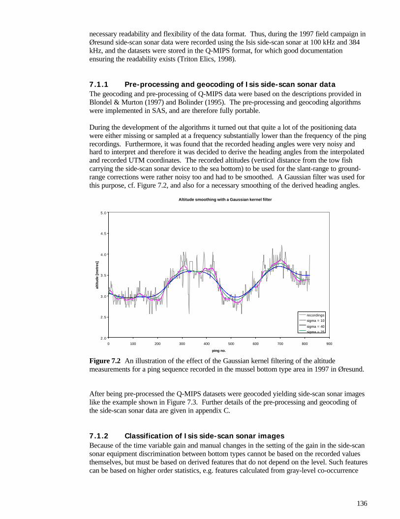
136

necessary readability and flexibility of the data format. Thus, during the 1997 field campaign inØresund side-scan sonar data were recorded using the Isis side-scan sonar at 100 kHz and 384kHz, and the datasets were stored in the Q-MIPS format, for which good documentationensuring the readability exists (Triton Elics, 1998).

7.1.1 Pre-processing and geocoding of Isis side-scan sonar dataThe geocoding and pre-processing of Q-MIPS data were based on the descriptions provided inBlondel & Murton (1997) and Bolinder (1995). The pre-processing and geocoding algorithmswere implemented in SAS, and are therefore fully portable.

During the development of the algorithms it turned out that quite a lot of the positioning datawere either missing or sampled at a frequency substantially lower than the frequency of the pingrecordings. Furthermore, it was found that the recorded heading angles were very noisy andhard to interpret and therefore it was decided to derive the heading angles from the interpolatedand recorded UTM coordinates. The recorded altitudes (vertical distance from the tow fishcarrying the side-scan sonar device to the sea bottom) to be used for the slant-range to ground-range corrections were rather noisy too and had to be smoothed. A Gaussian filter was used forthis purpose, cf. Figure 7.2, and also for a necessary smoothing of the derived heading angles.

Altitude smoothing with a Gaussian kernel filter

2.0

2.5

3.0

3.5

4.0

4.5

5.0

0 100 200 300 400 500 600 700 800 900

ping no.

altit

ude

[met

res]

recordingssigma = 10

sigma = 40sigma = 25

Figure 7.2 An illustration of the effect of the Gaussian kernel filtering of the altitudemeasurements for a ping sequence recorded in the mussel bottom type area in 1997 in Øresund.

After being pre-processed the Q-MIPS datasets were geocoded yielding side-scan sonar imageslike the example shown in Figure 7.3. Further details of the pre-processing and geocoding ofthe side-scan sonar data are given in appendix C.

7.1.2 Classification of Isis side-scan sonar imagesBecause of the time variable gain and manual changes in the setting of the gain in the side-scansonar equipment discrimination between bottom types cannot be based on the recorded valuesthemselves, but must be based on derived features that do not depend on the level. Such featurescan be based on higher order statistics, e.g. features calculated from gray-level co-occurrence

137

matrices, so-called GLCMs. GLCM methods are introduced in e.g. Haralick, Shanmugam &Dinstein (1973) and Carstensen (1992).

Figure 7.3 Resulting side-scan sonar image obtained from transect no. 23 in the Eelgrassbottom type area, 1997. (Gray levels have been inverted).

A discrimination based on global image features was carried out, for which 100 kHz and 384kHz side-scan sonar images from the three bottom type areas were selected; 3 images wereselected from the eelgrass bottom type area, and 2 images from the mussels and sand bottomtype areas, respectively. Based on the GLCMs for the selected side-scan sonar images 15 globalimage features were derived: Energy, entropy, maximum probability, correlation, diagonalmoment, kappa, difference energy, difference entropy, inertia, inverse difference moment, sumenergy, sum entropy, sum variance, cluster shade, and cluster prominence. Analyses ofvariance (ANOVA) were performed on these 15 features and revealed that the 100 kHz imagesdid a better job in the discrimination than the 384 kHz images, which was in accordance withthe impression of a visual inspection of the data.

Subsequently, geocoded images were classified by means of higher order local momentscalculated in a 7x7 filter window, and it was found that the discriminatory power resides mainly

138

with the second and third order moments (variance and skewness). Further details about the useof local moments for classification are given in the next section. One example of aclassification is shown in Figure 7.4, based on a resampling of the 0.25 x 0.25 m² pixels in theoriginal images into 1 x 1 m² pixels.

Figure 7.4 Geocoded 100 kHz Isis side-scan sonar image from the mussel bottom type area inØresund, 1997, and a segmentation hereof based on higher order local moments. Blue ismussels, yellow is sand and red is reject/other. The region covered by the images is 100 m by100 m.

7.2 Data fusion studiesThe data fusion carried out was aimed at the classification of the joint kriged echo sounder datafrom RoxAnn and side-scan sonar images. Side-scan sonar data entered into the classificationsonly via features derived from them. These are the abovementioned local second and thirdorder moments calculated in a 7x7 filter window. RoxAnn echo sounder data were kriged to a 1m grid. Only 100 kHz side-scan sonar images were used, as these seem to have the higherdiscriminatory power.

For the data fusion study to example datasets were chosen, namely the side-scan sonar pingsequence no. 103 from the mussel bottom type area, and the ping sequence no. 114 from thesand bottom type area. The echo sounder data consists of the datasets described in chapter 3and appendix B. The full side-scan sonar images (103) and (114) are shown in Figure 7.5 andFigure 7.6. For the classification the images were cropped to the specification areas applying tothe echo sounder data as well.

Two spatial resolutions were used, 25 cm and 1 meter. In the 25 cm case the mussel area imagecovers 560 x 568 pixels and the sand area image covers 400 x 400 pixels.

139

Figure 7.5 Geocoded Isis side-scan sonar images. The image to the left was produced from theping sequence 103, recorded at the location of the mussel bottom type area, and has an originalsize of 1200 x 1200 pixels. The image to the right was produced from the ping sequence 114,recorded at the location of the sand bottom type area, and has an original size of 800 x 800pixels.

All classifications described in the sequel were made by means of ordinary quadratic maximumlikelihood (ML) discriminant analysis, the same method as described in section 3.2. In all casesstatistics for the classifications were calculated only where all data, i.e. both echo sounder andside-scan sonar, have non-missing values. The results are shown as the classified images andthe resubstitution confusion matrices. In the Figures 7.6 - 7.11 the mussels area is shown on theleft and the sand area on the right. Missing data are coded white, mussels are blue, sand isyellow and rejects (beyond the 95% percentile in the χ2 distribution for the Mahalanobisdistance) are red.

140

RoxAnn data alone

Figure 7.6 Classification result for echo sounder data, 25 cm pixels. The mussel bottom typearea is depicted to the left and the sand bottom type area to the right, Øresund 1997. Blue ismussels, yellow is sand and red is reject class.

Figure 7.7 Classification result for echo sounder data, 1 m pixels. The mussel bottom type areais depicted to the left and the sand bottom type area to the right, Øresund 1997. Blue is mussels,yellow is sand and red is reject class.

Table 7.1 Resubstitution confusion matrix for echo sounder data, 25 cm pixels.Reject Mussels Sand Total

Mussels 5.90% 94.08% 0.02% 100%Sand 4.76% 1.06% 94.19% 100%Total 5.34% 48.32% 46.34% 100%

Table 7.2 Resubstitution confusion matrix for echo sounder data, 1 m pixels.Reject Mussels Sand Total


141

Side-scan Sonar data alone

Figure 7.8 Classification result for side-scan sonar data, 25 cm pixels. The mussel bottom typearea is depicted to the left and the sand bottom type area to the right, Øresund 1997. Blue ismussels, yellow is sand and red is reject class.

Figure 7.9 Classification result for side-scan sonar data, 1 m pixels. The mussel bottom typearea is depicted to the left and the sand bottom type area to the right, Øresund 1997. Blue ismussels, yellow is sand and red is reject class.

Table 7.3 Resubstitution confusion matrix for side-scan sonar data, 25 cm pixels.Reject Mussels Sand Total


Table 7.4 Resubstitution confusion matrix for side-scan sonar data, 1 m pixels.Reject Mussels Sand Total


142

Combined RoxAnn and SSS data

Figure 7.10 Classification result for combined echo sounder and side-scan sonar data, 25 cmpixels. The mussel bottom type area is depicted to the left and the sand bottom type area to theright, Øresund 1997. Blue is mussels, yellow is sand and red is reject class.

Figure 7.11 Classification result for combined echo sounder and side-scan sonar data, 1 mpixels. The mussel bottom type area is depicted to the left and the sand bottom type area to theright, Øresund 1997. Blue is mussels, yellow is sand and red is reject class.

Table 7.5 Resubstitution confusion matrix for combined echo sounderand side-scan sonar data, 25 cm pixels.

Reject Mussels Sand TotalMussels 6.52% 93.46% 0.02% 100%Sand 6.25% 0.89% 92.86% 100%Total 6.39% 47.92% 45.69% 100%

Table 7.6 Resubstitution confusion matrix for combined echo sounderand side-scan sonar data, 1 m pixels.

Reject Mussels Sand TotalMussels 6.95% 93.05% 0.00% 100%Sand 6.81% 1.02% 92.17% 100%Total 6.88% 45.33% 47.79% 100%

143

On the 1 m scale the satisfactory classification results are largely governed by the RoxAnn data,whereas for the 25 cm scale the finer resolution of the side-scan sonar data is conspicuous in theresulting image.

7.3 DiscussionOther surveyors and researchers have seemingly had similar experiences when comparing side-scan sonar to echo sounder based classification of the sea floor. Bornhold, Collins & Yamanaka(1999) conclude that side-scan images can provide a full coverage with good topographic detailand substrate information of varying quality, while the echo sounder data (QTC View in theircase) can provide detailed substrate classifications over a wide range of bottom types.

It remains an open problem to devise good recipes for the utilisation of side-scan sonar inclassification of smooth sea bottom textures like those formed by mussels and Cymodoceanodosa. For sea bottom textures containing objects at a scale making them clearly visible in theside-scan sonar images it is a more unproblematic task to classify the sea bed types, cf. thePosidonia oceanica patches present in Figure 7.1.

145

8 Models of spatial patterns

This chapter investigates the options for elaborating models of the spatial patterns formed bybenthic communities. The first section introduces relevant methods and pieces of theory, inparticular the Boolean model, and mentions some alternative frameworks for modelling ofspatial patterns. The second section describes how basic assumptions lead to the formulation ofa Boolean model for mussels, and outlines the same process for seagrasses. In the third sectiona new method for the estimation of non-stationary Boolean models is proposed, and the methodis illustrated for a side-scan sonar image of Posidonia oceanica.

8.1 IntroductionThis chapter gives some short bits and pieces regarding relevant fields like mathematicalmorphology, scale-space theory and stochastic geometry, and gives a short introduction toBoolean models. A short summary of other modelling frameworks for spatial patterns is given.

8.1.1 Mathematical morphologyThis subsection contains a short introduction to the basic operators used in mathematicalmorphology. The presentation relies on Serra (1982), Cressie (1991) and, in particular in thissection, on Vincent (1999).

The basic morphological operators are defined based on the concept of a structuring element,which is a particular set B ⊂ R2, usually small and of a simple shape like e.g. a disk, square or aline segment. The structuring element is translated over images X and its relationships with Xare studied at each location. An origin is supplied with the specification of the structuringelement B indicating the point in the B, which is used to position B in the image duringtranslations. An example of a square structuring element with the origin in the lower left corneris depicted in Figure 8.1.

•

Figure 8.1 A simple 3x3 square structuring element.

From B the transposed set B(

can be derived:

BbbB ∈−=(

B(

is derived by rotating B by 180o about the origin O, which typically belongs to B. Thetranslation of B by x is denoted by Bx:

146

BbxbBx ∈+=

The dilation of a set X ⊂ R2 by structuring element B, denoted δB (X), is the set of points x ∈ R2

such that the translation of B by x has a non-empty intersection with set X:

δB (X) = x∈ R2 | X ∩ Bx ≠ Ø

It can be shown that the dilation of X by B is equal to the Minkowski Addition of X and B(

,denoted X ⊕ B

(:

BbXxbxBXXB

((∈∈+=⊕= ,)(δ

The morphological dilation is defined as a Minkowski addition by some authors, in particular inthe U.S. (Sternberg, 1986), however without any transposition of the structuring element, whilethe former definition is used by the French school (Serra, 1982). In practice, this distinction ismostly academic, since useful structuring elements B are typically symmetric: B

( = B.

The erosion of X by a structuring element B, denoted εB(X), is the set of points x ∈ R2 such thatthe translation of B by x is included in X:

εB(X) = x ∈ R2 | Bx ⊆ X

This definition of the erosion of X by B corresponds to the Minkowski subtraction of X and B(

:

εB(X) = X ? B(

= x∈ R2 | ∀b ∈ B(

, x - b ∈ X

In popular terms the dilation operator tends to "grow" sets while the erosion "shrinks" them.Through dilation, different components of a set X can be connected and some holes and gapscan be filled, whereas with erosion holes become bigger, and objects (i.e. connectedcomponents) can vanish. More formally, these operations are equipped with a number offundamental properties, which will not be detailed here.

From the erosion and dilation operators, two other useful morphological transformations can bederived as follows:

The opening of X by B, denoted by γB (X), is given by:

))(()( XX BBB εδγ (=

The opening of X by B is often denoted by (X) B, or X ? B.

The closing of X by B, denoted by φB (X), is given by:

))(()( XX BBB δεφ (=

In the literature, the closing of X by B is sometimes denoted by (X) B or X ? B.

Openings and closings tend to smooth the boundary of the original set X, but each in a differentmanner. The opening tends to remove the small protrusions in which the structuring element

147

cannot fit, whereas the closing fills in the gaps that cannot hold the structuring element. Theopening also shrinks the original set whereas the closing makes it bigger. More formally, onecan state the following properties:

1. Openings and closings are increasing operators.2. Openings are anti-extensive, closings are extensive.3. Openings and closings are duals of each other.4. Openings and closings are idempotent.

A thorough exposition of mathematical morphology is given in Serra (1982), and a more recentintroduction to mathematical morphology is given by Vincent (1999).

8.1.2 Scale-space theoryScale-space theory deals with the problem of finding proper scales for processing of imageswith regard to some stipulated objectives. The scale is found by investigating the scale-spaceover an image, which consists of all smoothed versions of the image for a specified smoothingkernel and a smoothing parameter, t, denoting the position in scale-space. Usually a Gaussiankernel is used to generate the Gaussian scale-space over an image, and the scale parameter, t,can be defined as t = σ² where σ² is the variance parameter entering the Gaussian kernel. Thus,for an image I given by I: R² → R, the scale-space above it parameterised by t is given by

L(t) = g(t) ⊗ I,

where L: R² × R → R maps an image I into scale-space by smoothing it with the Gaussiankernel g(t), and ⊗ is the convolution operator.

One of the points of Gaussian scale-space theory is that it makes the use of geometric operatorslike differential operators very handy due to the properties of the Gaussian kernel. A goodintroduction to scale-space theory can be found in Lindeberg (1996).

8.1.3 Boolean modelsBoolean models are composites made by combining every point in a sample generated by ahomogeneous spatial Poisson point process with a compact set, which can be deterministic ordrawn from some distribution; the Boolean model then consists of the union of the compactsets. In the terminology of Boolean models the points, s, from the spatial Poisson process D aregerms and the compact sets, Z, assigned to the germs are grains. The Boolean model, X, is thengiven by

X = ∪ Zi ⊕ si | si ∈ D,

where the Minkowski addition Zi ⊕ si of the compact set Zi and the point si implies that Zi istranslated to have its origin located on si. The Poisson process is described by its intensity, λ,and the distribution of grains can be characterised by the expectation of the grain areas, E(|Z|),and e.g. the mean perimeter, E(P(Z)).

The mathematical treatment of Boolean models makes substantial use of the hitting functiondefined by

TX(K) = PX ∩K ≠ ∅

and its complement

QX(K) = 1-TX(K) = PX ∩K = ∅

148

where K can be interpreted as a structuring element. If K is a point, i.e. K = s, then themeasure q = QX(s) = 1 - Ps ∈ X is called the porosity of the Boolean model. The porosityis the probability that a point belongs to the complement of the Boolean model X. It can beshown, that

q = exp(-λE(|Z|)),

which is known as the coverage property of the Boolean model.

Introductions to Boolean models are given in Hall (1988), Cressie (1991) and Molchanov(1999).

8.1.4 Other frameworks for modelling of spatial patternsDeterministic spatial models could be established based on biogeochemical properties of thebenthic community in question, i.e. using dynamics of biota behaviour at the scale ofindividuals or at some aggregated scale to simulate temporal development and stability ofspatial patterns that might emerge. For example, a mussel pattern model might be formulatedusing a settling of larvae as an initial event and then applying simple rules guiding themovements of the growing mussels at the sea bed like e.g. substrate preferences and tendenciesto cluster. Simulating such a model over a sufficient time span might reveal patterns that couldprovide insight in the real world phenomena of mussel beds.

Reaction-diffusion models (Murray, 1993) based on Turing diffusion (Barrio et al., 1999) orsome other diffusion mechanism would be a strong alternative. These models are able tocapture a broad scope of pattern phenomena, ranging from the formation of spots on a leopardto the spatial patterns of epidemic outbreaks (Murray, 1993). Although stochastic diffusionmodels seem to be good candidates for modelling of spatial patterns, they were not used heredue to their complexity, especially in regard to estimation (Guttorp, 1995).

A successful application of a diffusion model to the development and structure of tidal musselpatches is described in Paine & Levin (1981). However, the spatial aspect of the mussel patchesis not included in that model.

Snover & Commito (1998) apply a fractal model to sea floor photos of mussels to obtainestimates of fractal dimensions of mussel patches and they obtain seemingly good andreasonable results. Stoyan (1994) recommends caution when fractal models are imposed onnatural phenomena perceived as point processes and demonstrates how second-ordercharacteristics of some point processes that are not self-similar can behave exactly as second-order characteristics for self-similar point patterns. A good introduction to the practicalapplication of fractals in the study of natural phenomena is given in Hastings & Sugihara(1993). Guillaudeux & Maillard (1998) used fractal models to simulate seabed textures andproduced ripple simulations that are visually adequate.

Exotic alternatives include the use of artificial life models. An artificial life model might applymaking use of internal states of individuals and the resulting actions-reactions to theenvironmental conditions and other individuals, including the clumping of individuals.

In the sequel the presentation is focused on simple stochastic models of spatial patterns like theBoolean model.

149

8.2 Models of spatial patterns for musselsThis section outlines the steps in deriving a model of spatial patterns for mussels, anddemonstrates some of the data material that might eventually be used to estimate such models.

8.2.1 Basic formulation of a spatial pattern model for musselsContemplating a little on the basic elements of the process under consideration, namely themussels, a description of a set of mussels can be given by

M = mi | i=1..N,where

mi = (si,pi), si ∈ R4

and the i'th mussel, mi, is given by its position si and property vector pi = (size, orientation, …).The set M will normally describe mussels within a certain local region, given by e.g. the UTMcoordinates of the corner points.

Leaving out all elements of the property vector but the size of the mussels, M can be projectedonto R² × R, i.e.

M → M’ = ((x,y)i, ri) | i=1..N,

keeping the geographical location (x,y)’ and leaving out altitude and temporal dynamics, andrepresenting the size of the mussel by a canonical measure like the length along the major axisof the shell, r. A grown Mytilus edulis measures 5 – 7 cm in the longer direction, and has a notentirely symmetric shape, however the deviation from symmetry is quite small and the spatialcontour of a mussel might well be modelled by an ellipse. Yet, to simplify matters it is chosento regard mussels as circular items in the following.

Assuming positions si to be members of a homogeneous Poisson process, M’ is a Booleanmodel of the spatial mussel pattern, where the mussel contours are the grains and their positionsare the germs. For general usage the assumption of a homogeneous Poisson process is nottenable (above a certain small scale), and therefore models must be found that allow theintensity of the point process to fluctuate. Within mussel beds a Boolean model based on aPoisson cluster process (Neyman-Scott process) might be an appropriate model at thefundamental scales.

Recent developments in models for spatial processes to be considered include the area-interaction model (Kendall, 1998) and the continuum random-cluster model. However, notrestricting the scope unnecessarily, it is simply assumed here that the intensities can fluctuateand exhibit spatial trends, and therefore a non-stationary Boolean model is suggested as a propermodel for spatial patterns of mussels.

Spatial models for seagrassesThe same elaboration as made above for mussels can be made for neptune grass leading to anon-stationary Boolean model too. However, there is a slight difference, as the grains for thePosidonia model would consist of neptune grass patches, which consist of one or several plantsand therefore not necessarily of individuals.

The video strip-charts depicted in Figure 8.2 are included for their visual appeal and their futurepotential for estimating models of spatial patterns for benthic communities at the fundamentalscales.

150

Figure 8.2 Video strip-charts from the field campaigns in Øresund.

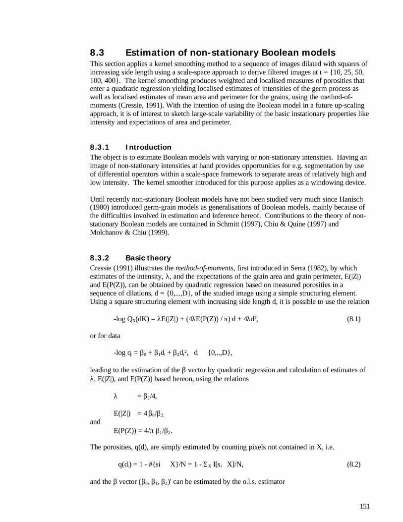
151

8.3 Estimation of non-stationary Boolean modelsThis section applies a kernel smoothing method to a sequence of images dilated with squares ofincreasing side length using a scale-space approach to derive filtered images at t = 10, 25, 50,100, 400. The kernel smoothing produces weighted and localised measures of porosities thatenter a quadratic regression yielding localised estimates of intensities of the germ process aswell as localised estimates of mean area and perimeter for the grains, using the method-of-moments (Cressie, 1991). With the intention of using the Boolean model in a future up-scalingapproach, it is of interest to sketch large-scale variability of the basic instationary properties likeintensity and expectations of area and perimeter.

8.3.1 IntroductionThe object is to estimate Boolean models with varying or non-stationary intensities. Having animage of non-stationary intensities at hand provides opportunities for e.g. segmentation by useof differential operators within a scale-space framework to separate areas of relatively high andlow intensity. The kernel smoother introduced for this purpose applies as a windowing device.

Until recently non-stationary Boolean models have not been studied very much since Hanisch(1980) introduced germ-grain models as generalisations of Boolean models, mainly because ofthe difficulties involved in estimation and inference hereof. Contributions to the theory of non-stationary Boolean models are contained in Schmitt (1997), Chiu & Quine (1997) andMolchanov & Chiu (1999).

8.3.2 Basic theoryCressie (1991) illustrates the method-of-moments, first introduced in Serra (1982), by whichestimates of the intensity, λ, and the expectations of the grain area and grain perimeter, E(|Z|)and E(P(Z)), can be obtained by quadratic regression based on measured porosities in asequence of dilations, d = 0,...,D, of the studied image using a simple structuring element.Using a square structuring element with increasing side length d, it is possible to use the relation

-log QX(dK) = λE(|Z|) + (4λE(P(Z)) / π)⋅d + 4λd², (8.1)

or for data

-log qi = β0 + β1di + β2di², di ∈ 0,..,D,

leading to the estimation of the β vector by quadratic regression and calculation of estimates ofλ, E(|Z|), and E(P(Z)) based hereon, using the relations

λ = β2/4,

E(|Z|) = 4⋅β0/β2,

andE(P(Z)) = 4/π⋅β1/β2.

The porosities, q(d), are simply estimated by counting pixels not contained in X, i.e.

q(di) = 1 - #si ∈ X/N = 1 - ΣX I[si∈X]/N, (8.2)

and the β vector (β0, β1, β2)' can be estimated by the o.l.s. estimator

152

β* = (T'T)-1T'Y,

where T is the matrix containing D row vectors (1, di, di²) and Y holds negative logarithms ofthe observed porosities, qi.

The method-of-moments can be extended to non-stationary Boolean models by calculating alocalised value of the porosities, qi(s), in every image pixel, s, thereby replacing the globalmeasures qi in (8.1) by localised weighted sums, where the weights stem from a Gaussian kernelapplied to the dilated image sequence. The kernel smoothing of the porosities is illustrated inFigure 8.3, and can be expressed as

q(s;di) = 1 - ΣX g(si-s)⋅I[si∈X]/N, (8.3)where

g(∆,t) = (4πt)-1/2 exp(-∆²/4t),

and t = σ² is the scale-space parameter. Thus, in every point, s, in the image the followingmodified version of the relation (8.1) is applied

-log QX(dK;s) = λ(s)E(|Z|;s) + (4λ(s)E(P(Z);s) / π)⋅d + 4λd², s ∈ image, (8.4)

and the object is to estimate the images reflecting λ(s), E(|Z|;s) and E(P(Z);s).

Figure 8.3 An illustration of the kernel smoothing. To the right, the global image isdepicted reflecting the constant weights employed when forming a global porositymeasure. To the left, the weights applied to the pixel at (60,40) by a Gaussian kernelwith a σ = 10 is illustrated.

Other estimation methods for non-stationary Boolean models reported in recent literatureinclude use of a certain combination of two structuring elements (Schmitt, 1997) and a anothermethod based on kernel smoothing of measures derived by the method of intensities(Molchanov & Chiu, 1999).

8.3.3 Illustration of the estimation method for Posidonia oceanicaA subset of a mosaic for Posidonia oceanica was extracted and classified manually bythresholding gray levels into binary pixels having the black representing Posidonia patches andwhite being sand, cf. Figure 8.4.

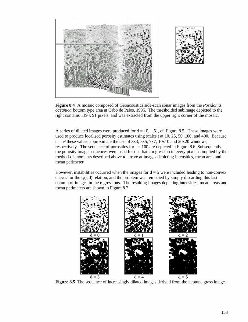
153

Figure 8.4 A mosaic composed of Geoacoustics side-scan sonar images from the Posidoniaoceanica bottom type area at Cabo de Palos, 1996. The thresholded subimage depicted to theright contains 119 x 91 pixels, and was extracted from the upper right corner of the mosaic.

A series of dilated images were produced for d = 0,...,5, cf. Figure 8.5. These images wereused to produce localised porosity estimates using scales t at 10, 25, 50, 100, and 400. Becauset = σ² these values approximate the use of 3x3, 5x5, 7x7, 10x10 and 20x20 windows,respectively. The sequence of porosities for t = 100 are depicted in Figure 8.6. Subsequently,the porosity image sequences were used for quadratic regression in every pixel as implied by themethod-of-moments described above to arrive at images depicting intensities, mean area andmean perimeter.

However, instabilities occurred when the images for d = 5 were included leading to non-convexcurves for the qi(s;d) relation, and the problem was remedied by simply discarding this lastcolumn of images in the regressions. The resulting images depicting intensities, mean areas andmean perimeters are shown in Figure 8.7.

d = 0 d = 1 d = 2

d = 3 d = 4 d = 5Figure 8.5 The sequence of increasingly dilated images derived from the neptune grass image.

154

d = 0 d = 1 d = 2

d = 3 d = 4 d = 5Figure 8.6 The sequence of increasingly smoothed porosity images estimated by Gaussiankernel smoothing with a parameter t = 100 of the increasingly dilated neptune grass images.

t = 10 t = 25 t = 50 t = 100 t = 400

Intensities

Areas

Perimeters

Figure 8.7 The resulting images of intensities, areas and perimeters for the scale parameters tused in the Gaussian kernel smoothing. The black holes in the images indicate regions ofsingularity in the o.l.s. estimator for the quadratic regression.

The results shown in Figure 8.7 indicate that the smoothing scale has to be sufficiently high toexclude local singularities. Furthermore, they show traces of resonance patterns around sharpthresholds in the data image, cf. the two ellipse-shaped contours that prevails up to t = 100 inthe images. Yet for t = 400 corresponding approx. to a 20x20 smoothing window the resultingimages are stable and give good indications of the spatial trends in intensities of the germs andthe shape distribution for the grains, cf. Figure 8.4.

155

The method proposed here might pose some challenges in terms of interpretability, on the otherhand it provides a high degree of resolution and detail, and therefore provides a good foundationfor the further use of spatial trends of the parameters in the non-stationary Boolean models.

For example, these models could be employed in the distribution mapping by means of up-scaling (Schneider et al., 1997) and kriging of the intensity field, possibly as an elaboration ofthe approach taken in Rathbun & Cressie (1994).

157

9 Summary and conclusions

This chapter contains a brief summary of the results and findings of the present study.

Chapter 3 outlined and detailed the necessary geostatistical data processing steps to preparedistribution maps based on echo sounder data. Based on exploratory spatial data analysessummarised in appendix B, this chapter demonstrated the feasibility of conducting classificationof feature spaces of echo sounder measurements and arrived at a hybrid block kriging methodproviding mussel coverage rates that were subsequently used to prepare spatial distributionmaps. Chapter 4 applied the algorithms developed and presented for mussels (Mytilus edulis) tothe mapping of neptune grass (Posidonia oceanica) and Cymodocea nodosa in theMediterranean and demonstrated that the method worked satisfactorily for the latter, which hasa smooth texture.

Chapter 5 demonstrated how geostatistical simulations could be used to assess the variability ofmussel distribution maps and the derived distribution areas of mussels. Chapter 6 demonstratedan alternative approach to the assessment of variability based on the use of Markov randomfields. Due to large amounts of missing data inherent in the transect based images an adjustedmethod for Ising model estimation called penalised maximum pseudo-likelihood (PMPL) wereproposed. A synthetic image thinning experiment demonstrated the feasibility of the methodand, in particular, its ability to control inflation of estimates caused by the large amount ofmissing data. Subsequently, it was demonstrated how the Ising field could be simulated toassess distribution map variability, and the results were compared to those obtained with thegeostatistical simulations.

Chapter 7 gave a short presentation of the use of side-scan sonar data and the fusion hereof withecho sounder data.

Chapter 8 discussed the formulating of models of spatial patterns formed by benthiccommunities and developed a new method to estimate localised parameters for non-stationaryBoolean models based on a combination of scale-space theory and the so-called method-of-moments for stationary Boolean models. The use of the proposed method was illustrated for thespatial patterns of Posidonia oceanica.

9.1 ConclusionsHere is a short discussion of the degree of fulfilment attained for the objectives of this Ph.D.study as they were outlined in section 1.1:

1) To determine the feasibility and applicability of hydroacoustic measurements in the form ofecho sounder recordings and side-scan sonar images for preparation of distribution mapsof benthic communities.

158

It has been shown that mussels can be quantified based on echo sounder measurements,provided a sufficiently elaborate methodology for the preparation of distribution maps is usedinvolving bottom type areas and groundtruth data to allow proper feature space classification.

For side-scan sonar data the use of higher order local moments (local standard deviations andlocal skewness) enabled classification and quantification for mussels, in particular when usedjointly with echo sounder data.

2) To develop statistically sound data processing methods for preparation of distribution mapson the basis of hydroacoustic measurements.

This is demonstrated and discussed in chapters 3 and 4.

3) To develop statistical methods for assessment of the uncertainty of distribution maps, inparticular of derived coverage area estimates.

Two approaches has been illustrated and their properties discussed in chapters 5 and 6, namelygeostatistical simulation and the use of Markov random fields in an MCMC setting, the latterexemplified by the use of an Ising model.

4) To suggest and estimate stochastic models of the spatial patterns of the selected benthiccommunities.

The case has been made that non-stationary Boolean models would provide a good startingpoint regarding stochastic models of spatial patterns for benthic communities, and a newestimation method has been proposed for such models.

9.2 Outlook and perspectivesSome issues of further research and development within the field of hydroacoustic marinebiology are briefly mentioned here.

♦ Multi-beam echo sounder and multi-beam sonar data are highly interesting and might turnout to be the primary instrumentation to use in the sea floor mapping in shallow waters.

♦ Up-scaling methods aimed at the combination of data sources (with different scales ofsupport and modelling regimes) into coherent distribution maps would be very interesting toapply to the methodologies and fields touched upon in this thesis.

The up-scaling could be based on a unified view of the spatial statistical methods, which ishinted at in the following table:

FrameworkInstantiation /

subfield / exampleSmooth /

MeanRough /

Covariance descriptors

Geostatistics Ordinary kriging Gaussian mean field, µ Variograms, γ(h)

Markov random fields Ising model logit mean field, α Energy coefficients, β

Stochastic geometry Boolean model Intensity field, λ Point and set covariancefunctions, C(h)

159

10 References

Adler R. (1981): The geometry of random fields. Wiley, New York.

Augustin J.M., le Suave R., Lurton X., Voisset M., Dugelay S. & Satra C. (1996): Contributionof the multibeam acoustic imagery to the exploration of the sea-bottom. MarineGeophysical Researches, Vol. 18, pp. 459-486.

Augustin N.H., Mugglestone M.A. & Buckland S.T. (1998): The role of simulation inmodelling spatially correlated data. Environmetrics, Vol. 9/2, pp. 175-196.

Balestri E., Piazzi L. & Cinelli F. (1998): Survival and growth of transplanted and naturalseedlings of Posidonia oceanica (L.) Delile in a damaged coastal area. Journal ofExperimental Marine Biology and Ecology, Vol. 228, pp. 209-225.

Barnes R.S.K. & Mann K.H. (1991): Fundamentals of aquatic ecology. 2. edition, BlackwellScientific Publications Ltd., Oxford.

Barrio R.A., Varea C., Aragón J.L. & Maini P.K. (1999): A two-dimensional numerical study ofspatial pattern formation in interacting turing systems. Bulletin of mathematicalbiology, Vol. 61, pp. 483-505.

Basford D.J., Eleftheriou A., Davies I.M., Irion G. & Soltwedel T. (1993): The ICES North SeaBenthos Survey: The Sedimentary Environment. ICES Journal of Marine Science, Vol.50, pp. 71-80.

Beauchemin S.S. & Barron J.L. (1995): The computation of optical flow. ACM ComputingSurveys, Vol. 27/3, pp. 433-467

Berkhout R.J., Chessa A.G. & Martinius A.W. (1996): A Statistical Adjustment of Haldorsen'sConditioned Boolean Simulation Algorithm. Mathematical Geology, Vol. 28/6, pp.791-810.

Besag J. (1974): Spatial interaction and the statistical analysis of lattice systems (withdiscussion). Journal of the Royal Statistical Society, Vol. 2, pp. 192-236.

Besag J. (1989): Towards Bayesian image analysis. Journal of Applied Statistics, Vol. 16/3, pp.395-407.

Besag J., Green P., Higdon D. & Mengersen K. (1996): Bayesian computation and stochasticsystems. Preprint.

Blondel P. & Murton B.J. (1997): Handbook of seafloor sonar imagery. Wiley, Chichester.

Blondel P., Parson L.M. & Robigou V. (1998): TexAn: Textural analysis of sidescan sonarimagery and generic seafloor characterisation. Proceedings of the IEEE Oceans '98Conference, pp. 419-423.

Bolinder A. (1995): Geographic rectification and mosaicking of side-scan sonar imagery. Ph.d.thesis, Department of Naval Architecture and Ocean Engineering, Chalmers Universityof Technology, Göteborg, Sweden.

160

Bornhold B.D., Collins W.T. & Yamanaka L. (1999): Comparison of seabed characterisationusing sidescan sonar and acoustic classification techniques. Canadian CoastalConference, Victoria, British Columbia, Canada.

Bozzano R., Mantovani R., Siccardi A. & Castellano L. (1998): Acoustic backscattering frommarine vegetation. Proceedings of the IEEE Oceans '98 Conference, pp. 1017-1021.

Brinke W.B.M ten, Augustinus P.G.E.F. & Berger G.W. (1995): Fine-grained SedimentDeposition on Mussel Beds in the Oosterschelde (The Netherlands), Determined fromEchosoundings, Radio-isotopes and Biodeposition Field Experiments. Estuarine,Coastal and Shelf Science, Vol. 40, pp.195-217.

Buckland S.T. (1982): A note on the Fourier series model for analysing line transect data.Biometrics, Vol. 38, pp. 469-477.

Burns D.R. (1992): Acoustic and elastic scattering from seamounts in three dimensions – Anumerical modeling study. J. Acoust. Soc. Am., Vol. 92/5, pp. 2784-2791.

Burns D., Queen C.B. & Chivers R.C. (1985): An ultrasonic signal processor for use inunderwater acoustics. Ultrasonics, July 1985, pp. 189-191.

Caccia D.C. (1998): Analyzing exact fractal time series: Evaluating dispersional analysis andrescaled range methods. Masters thesis, Statistics Department, University ofWashington.

Carstensen J.M. (1992): Description and simulation of visual texture. Ph.d. thesis, Departmentof Mathematical Modelling, Technical University of Denmark.

Cervenka P., Herzfeld U.C. & de Moustier C. (1994): Accuracy of the spatial representation ofthe seafloor with bathymetric sidescan sonars. Marine Geophysical Researches, Vol. 16,pp. 407-425.

Chauvaud S., Bouchon C. & Manières R. (1998): Remote sensing techniques adapted to highresolution mapping of tropical coastal marine ecosystems (coral reefs, seagrass beds andmangrove). Int. Journal of Remote Sensing, Vol. 19/18, pp. 3625-3639.

Cherry S. (1997): Non-parametric estimation of the sill in geostatistics. Environmetrics, Vol. 8,pp 13-27.

Chiu S.N. & Quine M.P. (1997): Central limit theory for the number of seeds in a growth modelin 3d ith inhomogeneous Poisson arrivals. The Annals of Applied Probability, Vol. 7/3,pp. 802-814.

Chivers R.C. & Burns D. (1991): Remote acoustic sensing of the seabed. Proceedings of the IVInternational School and Physical Acoustics, pp. 343-353, edited by A. Alippi. WorldScientific Publishers, Singapore.

Chivers R.C., Burns D. R. & Sisk H. (1989): Analysis of echo-sounder signals for sea-bedcharacterization. Ultrasonic International 89 Conference Proceedings.

Chivers R.C., Emerson N. & Burns D.R. (1990): New acoustic processing in underwaysurveying. The Hydrographic Journal, Vol. 56, pp. 9-17.

Cochran W.G. (1983): Planning and Analysis of Observational Studies. New York: John Wiley& Sons.

Cohen J. (1988): Statistical power analysis for the behavioral sciences. 2nd ed., LawrenceErlbaum Associates.

Collins W.T. & McConnaughey R.A. (1998): Acoustic classification of the sea floor to addressessential fish habitat and marine protected area requirements. Canadian HydrographicConference 1998, CHS, Victoria, British Columbia, Canada.

161

Collins W.T., Gregory R. & Anderson J. (1996): A Digital Approach to Seabed Classification.Sea Technology, August 1996.

Conradsen K. & Carstensen J.M. (1998): Markov random fields. Course notes for 04351:Statistical Image Analysis. Department of Mathematical Modelling, TechnicalUniversity of Denmark.

Conradsen K. (1984): An Introduction to Statistics; Vol 1A, 1B, 2A & 2B. Department ofMathematical Modelling, Technical University of Denmark.

Constantine A.G. & Hall P. (1994): Characterizing surface smoothness via estimation ofeffective fractal dimension. J.R. Statist. Soc., Vol. 56/1, pp 97-113.

Cox D.D., Cox L.H. & Ensor K.B. (1997): Spatial sampling and the environment: some issuesand directions. Environmental and Ecological Statistics, Vol. 4, pp. 219-233.

Cox D.R. & Miller H.D. (1965): The theory of stochastic processes. London, Chapman & Hall.

Cressie N. & Zimmerman D.L. (1992): On the stability of the geostatistical method.Mathematical Geology, Vol. 24/1, pp. 45-59.

Cressie N.A.C. (1991): Statistics for spatial data, John Wiley and Sons, Inc., New York, 900 pp.

Deutsch C.V. & Journel A.G. (1998): GSLIB, Geostatistical Software Library and User's Guide,second edition, Oxford University Press.

Diggle P.J, Tawn J.A. & Moyeed R.A. (1998): Model-based geostatistics (with discussion).Applied Statistics, Vol. 47/3, pp. 299-350.

Dolmer P. (1998): The interactions between bed structure of Mytilus edulis L. and the predatorAsterias rubens L. Journal of Experimental Marine Biology and Ecology, Vol. 228, pp.137-150.

Duarte C.M. & Sand-Jensen K. (1990): Seagrass colonization: Patch formation and patchgrowth in Cymodocea nodosa. Mar. Ecol. Progr. Ser., Vol. 65, pp. 193-200.

Dunning J.B, Stewart D.J., Danielson B.J., Noon B.R., Root T.L., Lamberson R.H.& StevensE.E. (1995): Spatially explicit population models: Current forms and future uses.Ecological Applications, Vol. 5/1, pp. 3-11.

Ersbøll B.K: (1989): Transformations and classifications of remotely sensed data - theory andgeological cases. Ph.d. thesis, Department of Mathematical Modelling, TechnicalUniversity of Denmark.

Fabricius-Bjerre, F. (1981): Textbook of Geometry, I: Analytical geometry and linear algebra.6th edition. In Danish. Polyteknisk Forlag.

Fismen M. (1997): Exact simulation using Markov chains. Master thesis, Norwegian Universityof Technology and Science, Trondheim, Norway.

Foley J.D., van Dam A., Feiner S.K. & Hughes J.F. (1990): Computer graphics, principles andpractice. 2. ed., Addison-Wesley, Reading, MA.

Foote K.G. & Stefánsson G. (1993): Definition of the problem of estimating fish abundanceover an area from acoustic line-transect measurements of density. ICES Journal ofMarine Science, Vol. 50, pp. 369-381.

Fox C.G. (1996): Objective classification of oceanic ridge-crest terrains using two-dimensionalspectral models of bathymetry: Application to the Juan de Fuca Ridge. MarineGeophysical Researches, Vol. 18, pp. 707-128.

Geman S. & Geman D. (1984): Stochastic relaxation, Gibbs distributions and the Bayesianrestoration of images. IEEE Transactions on Pattern Analysis and Machine Intelligence,Vol. 6, pp. 721-741.

162

Gensane M. (1989): A statistical study of acoustic signals backscattered from the sea bottom.IEEE Journal of Oceanic Engineering, Vol. 14/1, pp. 84-93.

Geyer C.J. & Thompson E. (1992): Constrained Monte Carlo maximum likelihood fordependent data (with discussion). Journal of the Royal Statistical Society, series B, Vol.54/3, pp. 657-699.

Geyer C.J. (1998): Likelihood inference for spatial point processes. Preprint.

Geyer C.J. (1999): Likelihood Inference for Spatial Point Processes. In Stochastic Geometry:Likelihood and Computation, eds. W. Kendall, O. Barndorff-Nielsen and M. N. M. vanLieshout, London: Chapman and Hall/CRC, pp. 141-172.

Gilks W.R., Richardson S. & Spiegelhalter D.J. (1996): Markov chain Monte Carlo in practice.Chapman & Hall.

Glasbey C.A. & Mardia K.V. (1998): A statistical framework for image warping. Preprint.

Goff J.A. & Jordan T.H. (1988): Stochastic modeling of seafloor morphology: Inversion of seabeam data for second-order statistics. Journal of Geophysical Research, Vol. 93/B11,pp. 13589-13608.

Green P.J. & Murdoch D.J. (1998): Exact sampling for Bayesian inference: towards generalpurpose algorithms. Bayesian Statistics, Vol. 6, Oxford University Press (Preprint).

Green P.J. (1998): Slides from a presentation outlining MCMC at the Strathclyde Conference,1998.

Green P.J. (1998a): Penalized likelihood. Preprint.

Green R. (1989): Power analysis and practical strategies for environmental monitoring.Environmental research, Vol. 50, pp. 195-205.

Guilladeux S. & Maillard E. (1998): Seabed simulations with fractal techniques. Proceedings ofIEEE Oceans '98 Conference, Vol. 1, pp. 433-437.

Guttorp P., Meiring W. & Sampson P.D. (1994): A space-time analysis of ground-level ozonedata. Environmetrics, Vol. 5, pp. 241-254.

Guttorp P. (1995): Stochastic Modeling of Scientific Data. Chapman & Hall / CRC.

Hall P. (1988): Introduction to the Theory of Coverage Processes. Wiley, New York.

Hanisch K.H. (1980): On classes of random sets and point process models. ElektronischeInformationsverarbeitung und Kybernetik, Vol. 16, pp. 409-412.

Haralick R.M., Shanmugam K. & Dinstein I. (1973): Textural featurs for image classification.IEEE Transactions on Systems, Man and Cybernetics, Vol. 3/6, pp. 610-621.

Hastings H.M. & Sugihara G. (1993): Fractals, a user's guide for the natural sciences. OxfordUniversity Press.

Hastings W.K. (1970): Monte Carlo sampling methods using Markov chains and theirapplications. Biometrika, vol. 57, pp. 97-109.

Hawrot R.Y. & Niemi G.J. (1996): Effects of edge type and patch shape on avian communitiesin a mixed conifer-hardwood forest. The Auk, Vol. 113/3, pp. 589-598.

Heald G.J. & Pace N.G. (1996): An analysis of 1st and 2nd backscatter for seabed classification.Proceedings of the 3rd European Conference on Underwater Acoustics. Heraklion,Crete, Greece. Ed. J. S. Papadakis.

Hellequin L. (1998): Statistical characterization of multibeam echosounder data. Proceedings ofthe IEEE Oceans '98 Conference, pp. 228-233.

163

Herzfeld, U.C., and Higginson C.A. (1996): Automated Geostatistical Seafloor Classification –Principles, Parameters, Feature Vectors, and Discrimination Criteria. Computers andGeoscience, Vol. 22, No. 1, pp. 35-52.

Higdon D.M. (1994): Spatial applications of Markov chain Monte Carlo for Bayesian inference.Ph.D. Dissertation, Statistics Department, University of Washington.

Hinkley D.V. (1988): Bootstrap methods. J. R. Statist. Soc. B, Vol. 50/3, pp. 321-337.

Hoelscher-Hoebing U. & Kraus D. (1998): Unsupervised image segmentation and image fusionfor multi-beam/multi-aspect sidescan sonar images. Proceedings of the IEEE Oceans '98Conference, pp. 571-576.

Hughes Clarke J.E., Mayer L.A. & Wells D.E. (1996): Shallow-water imaging multibeamsonars: A new tool for investigating seafloor processes in the Coastal Zone and on theContinental Shelf. Marine Geophysical Researches, Vol. 18, pp. 607-629.

Hughes J.P. & Guttorp P. (1994): Incorporating spatial dependence and atmospheric data in amodel of precipitation. Journal of Applied Meteorology, Vol. 33, pp. 1503-1515.

Huseby R.B., Milvang O., Solberg A.S. & Bjerde K.W. (1993): Seabed classification frommultibeam echosounder data using statistical methods. Proceedings of the IEEE Oceans'93 Conference, pp. 229-233.

Isaaks E.H. & Srivastava R.M. (1989): An introduction to applied geostatistics. OxfordUniversity Press, New York, 561 pp.

ISO 5725-2 (1994): Accuracy (trueness and precision) of measurements methods and results -Part 2: Basic method for the determination of repeatability and reproducibility of astandard measurement method. International Organization for Standardisation, Geneva.

Jiang M., Stewart W.K. & Marra M. (1993): Segmentation of seafloor sidescan imagery usingMarkov Random Fields and neural networks. Proceedings of the IEEE Oceans '93Conference, Vol. III, pp. 456-461.

Journel A. & Rossi M. (1989): When do we need a trend model in kriging? MathematicalGeology, Vol. 21/7, pp. 715-739.

Journel A.G. & Huijbregts C. (1978): Mining geostatistics. Academic Press.

Kaiser G. (1994): A Friendly Guide to Wavelets. Birkhäuser, Boston.

Kendall W. (1998): Perfect Simulation for the Area-Interaction Point Process. Preprint.

Kitanidis P.K. & Vomvoris E.G. (1983): A geostatistical approach to the inverse problem ingroundwater modeling (steady state) and one-dimensional simulations. WaterResources Research, Vol. 19/3, pp. 677-690.

Kleinbaum D.G. (1994): Logistic regression: A self-learning text. Springer-Verlag, New York.

Kostylev V., Erlandsson J. & Johannesson K. (1997): Microdistribution of the polymorphicsnail littorina saxatilis (Olivi) in a patchy rocky shore habitat. Ophelia, Vol. 47/1, pp 1-12.

Larsen R., Conradsen K. & Ersbøll B.K. (1998): Estimation of dense image flow fields in fluids.IEEE Transactions on Geoscience and Remote Sensing, Vol. 36/1, pp.256-264.

Laslett G.M. (1994): Kriging and splines: An empirical comparison of their predictiveperformance in some applications. Journal of the American Statistical Association, Vol.89/426, pp. 391-400.

Lindeberg T. (1996): Scale-space: A framework for handling image structures at multiplescales. Proceedings of Seminar at the CERN School of Computing, Egmond aan Zee,The Netherlands, 8-21 September, 1996.

164

Little S. A. & Smith D.K. (1996): Fault scarp identification in side-scan sonar and bathymetryimages from the Mid-Atlantic Ridge using wavelet-based digital filters. MarineGeophysical Researches, Vol. 18, pp. 741-755.

Lyngby J.E. & Sørensen P.S. (1994): Growth dynamics of eelgrass in Øresund and assessmentof impact of shading on eelgrass growth. Doc. No. 94/173/0E. Report toØresundskonsortiet prepared on behalf of VKI.

Magorrian B.H., Service M. & Clarke W. (1995): An acoustic bottom classification survey ofStrangford Lough, Northern Ireland. J. Mar. Biol. Ass. U.K., Vol. 75, pp. 987-992.

Malinverno A. (1989): Testing linear models of sea-floor topography. Pure and AppliedGeophysics, Vol 131, pp. 139-155.

Malladi R., Sethian J.A. & Vemuri B.C. (1994): Evolutionary fronts for topology-independentshape modeling and recovery. Proceedings of Third European Conference on ComputerVision (ECCV'94), Stockholm, Sweden, May 1994, pp. 3-13.

Mallet Y., Coomans D. & de Vel O. (1996): Recent developments in discriminant analysis onhigh dimensional spectral data. Chemometrics and Intelligent Laboratory Systems, Vol.35, pp. 157-173.

Maravelias C.D. & Haralabous J. (1995): Spatial distribution of herring in the Orkney/Shetlandarea (Northern North Sea): A geostatistical analysis. Netherlands Journal of SeaResearch, Vol. 34/4, pp. 319-329.

Marbá N., Duarte C.M., Cebrián J., Enríquez S., Gallegos M.E., Olesen B., Sand-Jensen K.(1996): Growth and population dynamics of Posidonia oceanica on the SpanishMediterranean coast: elucidating seagrass decline. Marine Ecology Progress Series,Vol. 137, pp. 203-213.

Martin E.B. & Scott E.M. (1995): The detection of change in spatial processes. Environmetrics,Vol. 6., pp. 141-154.

Martin-Löf A. (1973): Mixing properties, diferentiability of the free energy and the central limittheorem for a pure phase in the Ising model at low temperature. Comm. Math. Phys.,Vol. 32, pp. 75-92.



MAS3-CT95-0026 (1999): "Final Scientific Report of the BioSonar Project". Report preparedby the BioSonar project partners to the MAST Office of the European Union.

MAS-CT-0026 (1995): Technical annex to Sonar technology for monitoring and assessment ofbenthic communities. Prepared by the BioSonar project proposal group.

Messieh S.N., Rowell T.W., Peer D.L. & Cranford P.J. (1991): The effects of trawling, dredgingand ocean dumping on the eastern Canadian continental shelf seabed. Continental ShelfResearch, Vol. 11, Nos 8-10, pp. 1237-1263.

Molchanov I.S. (1999): Random closed sets. Chapter 7 contributed to Stochastic Geometry,Likelihood and Computation, edited by Barndorff-Nielsen, Kendall & van Lieshout,Chapman & Hall.

Molchanov I.S. & Chiu S.N. (1999): Smoothing techniques and estimation methods for non-stationary Boolean models with applications to coverage processes. Technical report,Department of Statistics, University of Glasgow.

Montgomery D.C: (1991): Design and analysis of experiments. 3rd edition, Wiley & Sons.

165

Murray J.D. (1993): Mathematical Biology. 2nd ed., Biomathematics Texts, Vol. 19, Springer-Verlag.

Myers D.E, Begovich C.L., Butz T.L. & Kane V. (1982): Variogram Models for RegionalGroundwater Geochemical Data. Mathematical Geology, Vol. 14, pp. 629-644.

Myers D.E. (1999): Book review: GSLIB, Geostatistical software library and user's guide,second edition; Clayton V. Deutsch and Andre G. Journel; Oxford University Press,1998, x + 369 pages, ISBN 0-19-510015-8. Computers & Geosciences, vol 25, pp. 309-312.

Nielsen A.A. (1994): Analysis of regularly and irregularly sampled spatial, multivariate, andmultitemporal data. Ph.d. thesis, Department of Mathematical Modelling, TechnicalUniversity of Denmark.

Nielsen A.A. (1996): Introduction to Geostatistics. Course notes to 8829: GeographicalInformation Systems. Department of Mathematical Modelling, Technical University ofDenmark.

Nielsen A.A. (1997): Linear unmixing. Research notes, Department of Mathematical Modelling,Technical University of Denmark.

Nielsen M. & Deriche R. (1996): Binocular dense depth reconstruction using isotropyconstraint. Proceedings of the 9th Scandinavian Conference on Image Analysis, pp. 49-56, Uppsala, Sweden, June 6-9 1995.

Nielsen M. (1998): Course notes for Statistical Image Analysis. Technical University ofDenmark, Spring 1998.

Nielsen M., Maas R., Niessen W.J., Florack L.M.J. & ter Haar Romey B.M. (1999): Binocularstereo from grey-scale images. Journal of Mathematical Imaging and Vision, Vol. 10/2,pp 103-122.

O'Driscoll R.L. (1998): Description of spatial pattern in seabird distributions along line transectsusing neighbour K statistics. Marine Ecology Progress Series, Vol. 165, pp. 81-94.

Onsager L. (1944): Crystal statistics, I. A two-dimensional model with an order-disordertransition. Phys. Rev., Vol. 65, pp. 117-149.

Pace N.G. & Dyer C.M. (1979): Machine classification of sedimentary sea bottoms. IEEETransactions of Geoscience Electronics, Vol. GE-17/3, pp. 52-56.

Paine R.T. & Levin S.A. (1981): Intertidal landscapes: Disturbance and the dynamics of pattern.Ecological Monographs, Vol. 51/2, pp. 145-178.

Parsons T.R., Takahashi M. & Hargrave B. (1977): Biological oceanographic processes. 2nd

edition, Pergamon Press, Oxford.

Parthiot F, Cervenka P. & Ollivier F. (1995): Seafloor spatial representation and bathymetrydata quality. IEEE Oceans '95 Conference Proceedings, Vol. 3, pp. 1922-1927.

Phillips D.L., Henry Lee E., Herstrom A.A., Hogsette W.E. & Tingey D.T. (1996): Use ofauxiliary data for spatial interpolation of ozone exposure in Southeastern forests.Environmetrics, Vol. 8, pp. 43-61.

Phinn S., Franklin J., Hope A., Stow D. & Huenneke L. (1995): Biomass distribution mappingusing airborne digital video imagery and spatial statistics in a semi-arid environment.Journal of Environmental Management, Vol. 47, pp. 139-164.

166

Pican N., Trucco E., Ross M., Lane D.M., Petillot Y. & Tena Ruiz I. (1998): Texture analysisfor seabed classification: Co-occurrence matrices vs self-organizing maps. Proceedingsof the IEEE Ocens '98 Conference, Vol. 1, pp. 424-428.

Pollock K.H. & Kendall W.L. (1987): Visibility bias in aerial surveys: A review of estimationprocedures. Journal of Wildlife Management, Vol. 51/2, pp. 502-510.

Porteiro C., Carrera P. & Miquel J. (1996): Analysis of Spanish acoustic surveys for sardine,1991-1993: abundance estimates and inter-annual variability. ICES Journal of MarineScience, Vol. 53, pp. 429-433.

Prager B.T., Caughey D.A. & Poeckert R.H. (1995): Bottom classification: operational resultsfrom QTC view. IEEE Oceans '95 Conference Proceedings, Vol. 3, pp. 1827-1835.

Pratson L.F. & Edwards M.H. (1996): Introduction to advances in seafloor mapping usingsidescan sonar and multibeam bathymetry data. Marine Geophysical Researches, Vol.18, pp. 601-605.

Press W.H., Teukolsky S.A., Vetterling W.T. & Flannery B.P. (1992): Numerical Recipes in C:The Art of Scientific Computing. 2. edition, Cambridge University Press.

Priebe R., Chotiros N.P., Walter D.J. & Lambert D.N. (1995): Sea Floor Classification byWavelet Decomposition of Fathometer Echoes. IEEE Oceans '95 ConferenceProceedings, Vol. 3, pp. 1814-1821.

Rathbun S.L. & Cressie N.A.C. (1994): Space-time survival point processes: Longleaf pines insouthern Georgia. Journal of the American Statistical Association, Vol. 89, pp. 1164-1174.

Rathbun S.L. (1998): Spatial modelling in irregularly shaped regions: Kriging estuaries.Environmetrics, Vol. 9/2, pp. 109-130.

Ripley B. (1988): Statistical inference for spatial processes. Cambridge University Press, NewYork, 1988.

Roberts E.A. (1993): Seasonal Cycles, Environmental Change and BACI Designs.Environmetrics, Vol. 4/2, pp. 209-231.

Rosholm A. (1997): Statistical methods for segmentation and classification of images. Ph.D.thesis, Department of Mathematical Modelling, Technical University of Denmark.

Rossi R.E., Mulla D.J., Journel A.G. & Frannz E.H. (1992): Geostatistical tools for modelingand interpreting ecological spatial dependence. Ecological Monographs, Vol. 2/2, pp.277-314.

Sabol B.M. & Burczinski J. (1998): Digital echo sounder system for characterizing vegetationin shallow-water environments. Proceedings of the Fourth European Conference onUnderwater Acoustics, edited by A. Alippi & G.B. Cannelli, Rome, 1998.

Sabol B.M., Shaffer D.J. & Melton jr. E. (1996): Mapping seagrasses for dredging operations.US Army Corps of Engineers. Vol D-96-1.

Sampson P.D. & Guttorp P. (1992): Nonparametric estimation of nonstationary spatialcovariance structure. Journal of the American Statistical Association, Vol. 87, pp. 108-119.

Schlagintweit G.E.O. (1993): Real-time acoustic bottom classification for hydrography – a fieldevaluation of RoxAnn. Proceedings of the IEEE Oceans '93 Conference, Vol. III, pp.214-219.

Schlese-Heidelbaugh W. & Nelson W.G. (1995): A power analysis of methods for assessmentof change in seagrass cover. Aquatic Botany, Vol. 53, pp. 227-233.

167

Schmitt M. (1997): Estimation of intensity and shape in a non-stationary Boolean model.Proceedings of the International Symposium "Advances in Theory and Applications ofRandom sets", October 9-11, 1996, Fontainebleau, France.

Schneider D.C., Walters R., Thrush S. & Dayton P. (1997): Scale-up of ecological experiments:Density variation in the mobile bivalve Macomona liliana. Journal of Experimentalmarine Biology and Ecology, Vol. 216, pp. 129-152.

Schultz N. & Ersbøll A. (1998): Meditteranean Rox Ann data. Data report, Department ofMathematical Modelling, Technical University of Denmark.

Schultz N. (1995): Segmentation and classification of biological objects. Ph.d. thesis,Department of Mathematical Modelling, Technical University of Denmark.

Schultz N. (1998): A Nonparametric deformable template classifier. Preprint.

Schultz N. (1999): Using a Nonparametric Deformable Template Classifier for Sea Floorsegmentation. Preprint.

Serra J. (1982): Image Analysis and Mathematical Morphology. Academic Press London.

Settle J.J. & Drake N.A. (1993): Linear mixing and the estimation of ground cover proportions.Int. Journal of Remote Sensing, Vol. 14/6, pp. 1159-1177.

Snover M.L. & Commito J.A. (1998): The fractal geometry of Mytilus edulis L. spatialdistribution in a soft-bottom system. Journal of Experimental Marine Biology andEcology, Vol. 223, pp. 53-64.

Sørensen P.S. (1994a): Sample sizes and power considerations for the Marine MonitoringProgramme. Report no. 94/126/0E to Øresundskonsortiet prepared on behalf of VKI.

Sørensen P.S. (1994b): The statistical basis for use of RoxAnn measurements to preparedistribution maps. Doc. No. 94/160/0E. Report to Øresundskonsortiet prepared onbehalf of VKI.

Sørensen P.S. (1995): Study of RoxAnn as a basis for mapping of mussel beds, Doc. no.95/109/1E. Report to Øresundskonsortiet prepared on behalf of VKI.

Sørensen P.S., Madsen K.N., Nielsen A.A., Schultz N., Conradsen K. & Oskarsson O. (1998):Mapping of the benthic communities Common mussel and Neptune grass by use ofhydroacoustic measurements. 3rd European Marine Science & Technology Conference,Session report of Seafloor characterisation session, European Commission.

Sotheran I.S., Foster-Smith R.L. & Davis J. (1997): Mapping of marine benthic habitats usingimage processing techniques within a raster-based geographic information system.Estuarine, Coastal and Shelf Science, Vol. 44/A, pp. 25-31.

Spencer S., Smith D.K., Cann J.R., Lin J. & McAllister E. (1997): Structure and stability ofnon-transform discontinuities on the Mid-Atlantic Ridge between 24o N and 30o N.Marine Geophysical Researches, Vol. 19, pp. 339-362.

Sternberg S.R. (1986): Grayscale morphology. Computer Vision, Graphics, and ImageProcessing, Vol. 35/3, pp. 333-355.

Stoyan D. (1982): A remark on the line transect method. Biom. J. Vol. 24/2, pp. 191-195.

Stoyan D. (1994): Caution with "fractal" point patterns! Statistics, Vol 25, pp. 267-270.

Sullivan P.J. (1991): Stock abundance estimation using depth-dependent trends and spatiallycorrelated variation. Can. J. Fish. Aquat. Sci., Vol. 48, pp. 1691-1703.

Swendsen R.H. & Wang, J.S. (1987): Nonuniversal critical dynamics in Monte Carlosimulations. Physical Review Letters, Vol. 58/2, pp. 86-88.

168

Switzer P. & Green A.A. (1984): Min/max autocorrelation factros for multivariate spatialimagery. Tech. rep. 6, Stanford University. 10 pp.

Tamsett D. (1992): Sea-bed characterisation and classification from the power spectra of side-scan sonar data. Marine Geophysical Researches, Vol. 15, pp. 43-64.

Tassan S. (1994): Local algorithms using SeaWiFS data for the retrieval of phytoplankton,pigments, suspended sediment, and yellow substance in coastal waters. Applied Optics,Vol 33/12, pp. 2369-2378.

Theisen B.F. (1977): Feeding rate of Mytilus edulis L. (Bivalvia) from different parts of Danishwaters in the water of different turbidity. Ophelia, Vol. 16/2, pp. 221-232.

Theisen B.F. (1982): Variation in size of gills, labial palps, and adductor muscle in Mytilusedulis L. (Bivalvia) from Danish waters. Ophelia, Vol. 21/1, pp. 49-63.

Thompson S.K. (1992): Sampling. John Wiley & Sons Inc.

Triton Elics Inc. (1998): Q-MIPS Data format description. Preprint.

Tukey J. (1977): Exploratory Data Analysis. Addison Wesley, Reading, MA.

Vincent L. (1999): Current topics in applied Morphological Image Analysis. Chapter 6contributed to Stochastic Geometry, Likelihood and Computation, edited by Barndorff-Nielsen, Kendall & van Lieshout, Chapman & Hall.

Weaver W. (1982): Lady Luck: The theory of probability. Dover edition, Dover PublicationsInc., New York.

Wen R. & Sinding-Larsen R. (1997): Image filtering by factorial kriging - sensitivity analysisand application to Gloria side-scan sonar images. Mathematical Geology, Vol. 28/4, pp.433-468.

Williamson N.J. & Traynor J.J. (1996): Application of a one-dimensional geostatisticalprocedure to fisheries acoustic surveys of Alaskan pollock. ICES Journal of MarineScience, Vol. 53, pp. 423-428.

Zietz S. & Elicker C. (1995): Modeling and analysis of sonar backscatter intensity for oceanbottom classification. Proceedings of the IEEE Oceans '95 Conference, pp. 1836-1839.

Spatial distribution maps for benthic communities

Documents

Transcript of Spatial distribution maps for benthic communities