Quantifying disturbances in benthic communities—comparison of the community disturbance index...

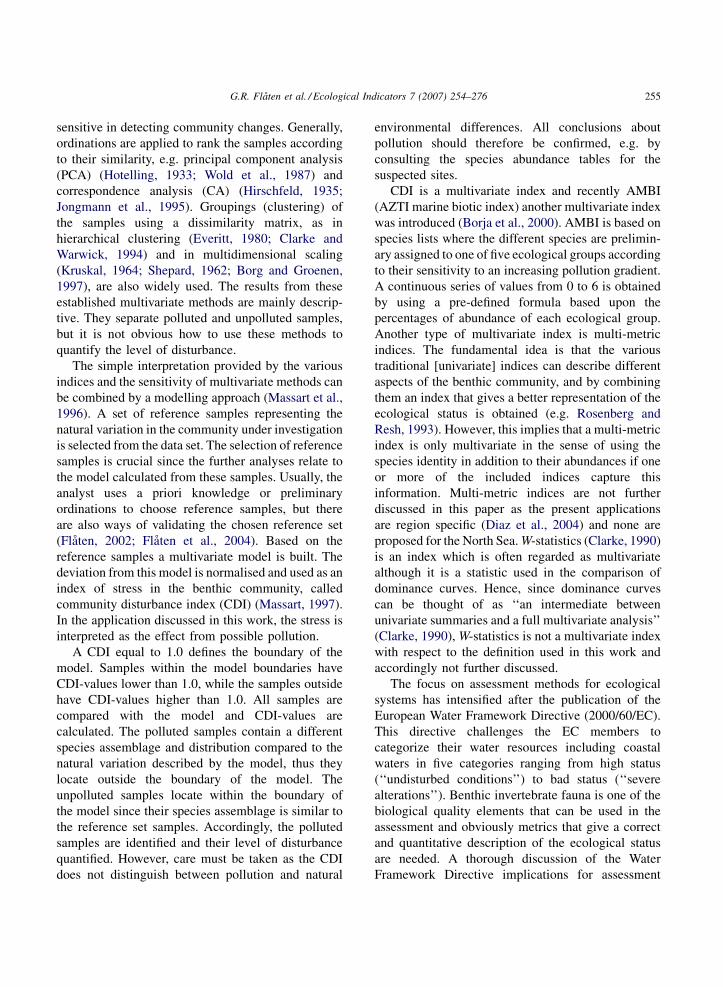
This article is also available online at:www.elsevier.com/locate/ecolind

Ecological Indicators 7 (2007) 254–276

Quantifying disturbances in benthic communities—comparison

of the community disturbance index (CDI)

to other multivariate methods

Geir Rune Flaten a,*, Helge Botnen b, Bjørn Grung a, Olav M. Kvalheim a

a Department of Chemistry, University of Bergen, Allegaten 41, N-5007 Bergen, Norwayb Section of Applied Environmental Research, Høyteknologisenteret, N-5020 Bergen, Norway

Received 30 March 2005; received in revised form 3 February 2006; accepted 5 February 2006

Abstract

A multivariate index assessing community stress in marine benthic count data is compared to other multivariate methods.

Both ordinations and clustering methods are included in the comparison and so is AMBI (AZTI marine biotic index). The

community disturbance index (CDI) requires the data to contain undisturbed reference samples. If this requirement is met, the

calculations are carried out in two steps. Firstly, the reference samples are separated and used to build a model representing the

natural variation. Subsequently, the remaining samples are compared to the model and the respective disturbance indices are

calculated. The CDI has the same sensitivity as the traditional multivariate methods. Additionally, one obtains a quantification of

the relative level of disturbance. The comparison is performed using data from monitoring surveys at three different oilfields in

the North Sea: Troll, Ekofisk and Oseberg-Brage. The samples are collected in 1996, 1990 and 1996, respectively.

# 2006 Published by Elsevier Ltd.

Keywords: Multivariate analysis; Environmental monitoring; Marine benthic analyses; Community disturbance index (CDI); Pollution

1. Introduction

Marine benthic communities are sensitive to

natural and anthropogenic factors in the local

environment. This is utilised in environmental impact

surveys where benthic fauna is widely used as an

indicator of pollution (e.g. Olsgard and Gray, 1995).

There are several ways to extract information from the

* Corresponding author. Fax: +47 55 58 94 90.

E-mail address: [email protected] (G.R. Flaten).

1470-160X/$ – see front matter # 2006 Published by Elsevier Ltd.

doi:10.1016/j.ecolind.2006.02.001

data collected in such surveys. Various indices may be

used, e.g. Shannon–Wiener (Shannon and Weaver,

1949), Pielou (Pielou, 1966) and Hurlbert (Hurlbert,

1971). All of them assign a single value (index) to each

sample. The indices are calculated from the abundance

of species and their distribution without considering

the species assemblage. Accordingly, community

changes due to differences in the species assemblage

are not detected by these indices.

Multivariate approaches utilise the species identity

in addition to their abundances. Thus, they are more

mailto:[email protected]

http://dx.doi.org/10.1016/j.ecolind.2006.02.001

G.R. Flaten et al. / Ecological Indicators 7 (2007) 254–276 255

sensitive in detecting community changes. Generally,

ordinations are applied to rank the samples according

to their similarity, e.g. principal component analysis

(PCA) (Hotelling, 1933; Wold et al., 1987) and

correspondence analysis (CA) (Hirschfeld, 1935;

Jongmann et al., 1995). Groupings (clustering) of

the samples using a dissimilarity matrix, as in

hierarchical clustering (Everitt, 1980; Clarke and

Warwick, 1994) and in multidimensional scaling

(Kruskal, 1964; Shepard, 1962; Borg and Groenen,

1997), are also widely used. The results from these

established multivariate methods are mainly descrip-

tive. They separate polluted and unpolluted samples,

but it is not obvious how to use these methods to

quantify the level of disturbance.

The simple interpretation provided by the various

indices and the sensitivity of multivariate methods can

be combined by a modelling approach (Massart et al.,

1996). A set of reference samples representing the

natural variation in the community under investigation

is selected from the data set. The selection of reference

samples is crucial since the further analyses relate to

the model calculated from these samples. Usually, the

analyst uses a priori knowledge or preliminary

ordinations to choose reference samples, but there

are also ways of validating the chosen reference set

(Flaten, 2002; Flaten et al., 2004). Based on the

reference samples a multivariate model is built. The

deviation from this model is normalised and used as an

index of stress in the benthic community, called

community disturbance index (CDI) (Massart, 1997).

In the application discussed in this work, the stress is

interpreted as the effect from possible pollution.

A CDI equal to 1.0 defines the boundary of the

model. Samples within the model boundaries have

CDI-values lower than 1.0, while the samples outside

have CDI-values higher than 1.0. All samples are

compared with the model and CDI-values are

calculated. The polluted samples contain a different

species assemblage and distribution compared to the

natural variation described by the model, thus they

locate outside the boundary of the model. The

unpolluted samples locate within the boundary of

the model since their species assemblage is similar to

the reference set samples. Accordingly, the polluted

samples are identified and their level of disturbance

quantified. However, care must be taken as the CDI

does not distinguish between pollution and natural

environmental differences. All conclusions about

pollution should therefore be confirmed, e.g. by

consulting the species abundance tables for the

suspected sites.

CDI is a multivariate index and recently AMBI

(AZTI marine biotic index) another multivariate index

was introduced (Borja et al., 2000). AMBI is based on

species lists where the different species are prelimin-

ary assigned to one of five ecological groups according

to their sensitivity to an increasing pollution gradient.

A continuous series of values from 0 to 6 is obtained

by using a pre-defined formula based upon the

percentages of abundance of each ecological group.

Another type of multivariate index is multi-metric

indices. The fundamental idea is that the various

traditional [univariate] indices can describe different

aspects of the benthic community, and by combining

them an index that gives a better representation of the

ecological status is obtained (e.g. Rosenberg and

Resh, 1993). However, this implies that a multi-metric

index is only multivariate in the sense of using the

species identity in addition to their abundances if one

or more of the included indices capture this

information. Multi-metric indices are not further

discussed in this paper as the present applications

are region specific (Diaz et al., 2004) and none are

proposed for the North Sea. W-statistics (Clarke, 1990)

is an index which is often regarded as multivariate

although it is a statistic used in the comparison of

dominance curves. Hence, since dominance curves

can be thought of as ‘‘an intermediate between

univariate summaries and a full multivariate analysis’’

(Clarke, 1990), W-statistics is not a multivariate index

with respect to the definition used in this work and

accordingly not further discussed.

The focus on assessment methods for ecological

systems has intensified after the publication of the

European Water Framework Directive (2000/60/EC).

This directive challenges the EC members to

categorize their water resources including coastal

waters in five categories ranging from high status

(‘‘undisturbed conditions’’) to bad status (‘‘severe

alterations’’). Benthic invertebrate fauna is one of the

biological quality elements that can be used in the

assessment and obviously metrics that give a correct

and quantitative description of the ecological status

are needed. A thorough discussion of the Water

Framework Directive implications for assessment

G.R. Flaten et al. / Ecological Indicators 7 (2007) 254–276256

methods is outside the scope of this paper although

some considerations are included in Section 5.

In the present work, the performance of the CDI is

compared to traditional multivariate approaches and

AMBI. In the first part of the theory section a brief

introduction to the tested multivariate methods is

given. The last part of the theory section contains a

thorough presentation of the CDI approach. This

includes a presentation of the modelling approach and

a suggestion of how CDI-values can be regarded in a

statistical context, as the CDI approach is expected to

be unfamiliar to the reader. In the results and

discussions sections comparisons are made for three

different data sets collected during environmental

monitoring surveys in the vicinity of oil platforms in

the North Sea. The data sets are chosen due to the

homogenous natural environment at each field and the

single source of disturbance, which creates a gradient

of decreasing disturbance with increasing distance to

the oil platform. These features simplify the validation

of the analysis results, although it is expected that

CDI-values can be used to quantify the environmental

stress or pollution level, in any surveys where samples

from unpolluted sites (i.e. reference set samples) exist.

2. Theory

2.1. Ordination methods

Ordination methods separate the samples due to

their species assemblage and abundance. The ordina-

tions are presented in plots where increasing distance

and angular deviations reflect increasing difference

among samples.

2.1.1. Principal component analysis

Principal component analysis (PCA), (Hotelling,

1933; Wold et al., 1987), is a decomposition of the

abundance matrix, X, into k components:

X ¼ TPt þ E (1)

where T and P are the score and loading matrices,

respectively. Both contain k column vectors. Super-

script t is used to denote transposition. The number of

principal components, k, is chosen according to the

criterion of maximal systematic variance explained.

Often, a k of two or three is sufficient to account for

most of the systematic variance among samples. The

scores and loadings are calculated by demanding

maximal explained variance under the constraint of

mutual orthogonality among the components. The

residual matrix, E, contains the part of X not explained

by the principal components.

2.1.2. Correspondence analysis

Correspondence analysis (CA) (Hirschfeld, 1935;

Jongmann et al., 1995) is a PCA with weighting:

M�1XN�1 ¼ TcaPtca þ E (2)

where both M and N are diagonal matrices. The

diagonal in M contains the row sums of the abun-

dance matrix, X, while N contains the column sums.

Tca and Ptca are the scores and loadings matrices,

respectively. They are labelled ‘ca’ to emphasise that

they are different from the PCA scores and loadings.

Two or three components are often sufficient to

explain most of the variation. As in Eq. (1), E is

the residual matrix.

2.2. Methods based on the dissimilarity matrix

The distances between the sample vectors, called

dissimilarities, can be used for grouping the data.

Bray–Curtis dissimilarities (Bray and Curtis, 1957)

are usually applied when analysing benthic count data,

and they are calculated as:

di j ¼Pn

k¼1 jxik � x jkjPnk¼1ðxik þ x jkÞ

; i; j ¼ 1; . . . ;m (3)

where dij is the dissimilarity between sample i and j, xik

the count of species k in sample i, m the number of

samples in the data set, and n is the number of species.

All the di,j-values are collected in a symmetric dis-

similarity matrix, D.

2.2.1. Multidimensional scaling

Non-metric multidimensional scaling (MDS)

(Kruskal, 1964; Shepard, 1962; Borg and Groenen,

1997) is a low-dimensional representation of the

information in the dissimilarity matrix. An MDS plot

is a mapping of the dissimilarities, dij, into the

corresponding distances, distij(Z), in an MDS space Z


(Borg and Groenen, 1997, p. 31):

f : di j! disti jðZÞ (4)

In order to assess the quality of the MDS models

the stress value proposed by Kruskal (1964) is used:

Stress ¼

ffiffiffiffiffiffiffiffiffiffiffiffiffiffiffiffiffiffiffiffiffiffiffiffiffiffiffiffiffiffiffiffiffiffiffiffiffiffiPðdi j � disti jðZÞÞ2P

d2i j

s(5)

Stress values measure the correspondence between the

mapping into the MDS space, distij(Z), and the dis-

similarities, dij. The lower the stress value, the better

the representation of the dissimilarities in the MDS

space, i.e. the corresponding MDS plot gives a better

picture of groupings and clusters in the data as cap-

tured by the dissimilarities. A rule-of-thumb is that

stress values above 0.2 indicate poor representation of

the data. Nevertheless, this is only suggestive since

both the numbers of samples and the properties of the

data influence the stress value.

2.2.2. Agglomerate hierarchical clustering

In agglomerate hierarchical clustering (Everitt,

1980; Johnson and Wichern, 1992) the two samples

having the smallest dissimilarity are identified and

joined. The dissimilarities containing the two com-

bined samples are removed from the dissimilarity

matrix. Subsequently, dissimilarities between the new

cluster of samples and the remaining samples are

calculated and inserted into the dissimilarity matrix.

This is repeated until all the samples are connected.

The sequence of combinations shows the groupings in

the data. This is visualised in a dendrogram.

Group average linking is usually applied to

calculate the new dissimilarities in benthic analyses.

It defines the dissimilarities of the new group as the

mean of the dissimilarities in the preceding groups,

and can be formulated as (Johnson and Wichern,

1992):

dðUVÞW ¼PNðUVÞ

i

PNW

k dik

NðUVÞNW

(6)

where d(UV)W is the new dissimilarity when combining

cluster (group) (UV) with cluster (sample) W. dik is the

distance between object i in UV and object j in W.

N(UV) and NW is the number of items in clusters (UV)

and W.

2.3. Modelling approach

The modelling approach consists of two steps: a

model describing the natural variation in the survey

area is built. Subsequently, the samples are compared

to this model and the similarity to the model is

quantified by the CDI-values. The samples outside the

boundaries of the model are classified as not belonging

to the model. They have a different species

assemblage, which is either due to pollution or

deviations in the natural environmental factors. The

boundaries of the model are determined by the F-

statistics, as shown later in this section (Eq. (10)).

The least complicated model is one single point. The

distance to this point determines whether a sample

belongs to the model. Confidence intervals are point

models. The upper and lower confidence limits

correspond to the boundaries of the model, while the

centre point represents the model. In Fig. 1a the (1 � a)

confidence interval for the standardised normal dis-

tribution is shown. The confidence interval is the part of

the probability density function labelled (1 � a). The a

samples within the shaded tails are outside the con-

fidence interval and hence outside the model. Observe

that the distance between a sample and the centre point

determinewhether that samples lies outside or inside the

confidence interval, i.e. outside or inside the model.

The point model can be extended to a line model,

and such a model is shown in Fig. 1b. Asterisks

indicate the model itself. The boundary for a line

model is a surrounding cylinder and in the figure the

solid lines indicate this boundary. Two hundred

simulated samples are compared with the model in

Fig. 1b. Each of the samples is indicated by a point.

The samples outside the boundary of the model are

emphasised by bold face. Obviously samples outside

the model can also be located in front of or behind the

cylinder which corresponds to the model boundary.

The histogram for the distances between the samples

and the line model in Fig. 1b, are shown in Fig. 1c. The

white bars represent the samples within the model

boundaries, while the shaded bars represent the samples

outside the boundaries, i.e. the samples indicated by

bold points in Fig. 1b. By definition, the distance

between a sample and the line model is always positive,

and therefore the histogram only contains positive

numbers. Observe that there is a clear similarity

between the right half of the probability density


Fig. 1. The figure outlines the idea of modelling by comparing modelling with the well-known confidence interval. (a) The probability function

for the standardised normal distribution is shown. The main part, labelled (1 � a), is the part of the distribution within the 100(1 � a)%

confidence interval. The confidence interval can be seen as a point model for the centre point, here zero. (b) A line model (asterisks) for a set of

measurements (points). The boundary of the model (solid cylinder) is found by statistical testing on the residuals for the samples. The distance to

the model determines whether a sample is inside or outside the model. It is a clear analogy to the confidence interval or point model shown in (a).

(c) The distribution of the distances to the model for the samples in (b). The vertical line indicates the boundary of the model, and the bars

representing samples outside the model are shaded. Observe the resemblance with the right half of the probabilities function in (a).


function in Fig. 1a and the histogram of the distances

to the model in Fig. 1c. The model is easily extended to

more dimensions.

2.3.1. Community disturbance index

The calculation of CDI-values is based on a

modelling approach called soft independent modelling

of class analogies (SIMCA) (Wold, 1976). In short, it is

a supervised classification where the models are built

using a lower dimensional representation (PCA) of a

reference set selected a priori. The reference set consists

of the sampling sites representing the natural variation,

i.e. the undisturbed sites. The a priori knowledge used to

select this reference set is generally the results from the

ordinations combined with the lists of the most

abundant species. The ordinations are used to separate

the reference samples, and the abundance lists are used

to identify them. The distance to the oil rig is an

additional parameter, which can be used to select

reference samples in the application presented in this

work as it is reasonable to expect that the pollution

impact decreases with increasing distance to the

pollution source (the oil rig). There are ways for

validating reference sets (Flaten, 2002), but these

approaches are not further discussed in this work.

A PCA model, describing the natural variation, is

built from the reference set (Eq. (1)).1 The number of

components to include in the model, k, is decided by

cross validation (Wold, 1978). In short, cross

validation is to successively remove groups of samples

from the reference set, building models of the

remaining samples with various numbers of compo-

nents and subsequently predicting the left out samples.

The number of components that gives the smallest sum

of squared prediction errors is used in the model of the

reference set. After the model has been found, new

samples are compared to it using:

ti ¼ xiPrefðPtrefPrefÞ�1

(7)

and

ei ¼ xi � tiPref (8)

1 Even though it is widely assumed that the PCA requires normal-

ity in the data, the development of principal components does not

require a multivariate normal assumption (Johnson and Wichern,

1992). The benthic count data form sparse integer matrices, but for

modelling purposes PCA seems to handle this kind of data.

where xi is the sample to be compared to the model,

Pref the loading matrix for the reference set, and ti is

the vector containing the estimated scores for sam-

ple i. The residual, ei, contains the variation in xi not

accounted for by the model. The line model example

in Fig. 1c can be regarded as a SIMCA model

with one component, and in that case the residual

corresponds to the distance from the sample to the

model.

To assess the samples within or outside the

boundary of the model, the residual standard deviation

(RSD) is used. Firstly, the RSD-value for each sample

i belonging to the reference set is calculated as:

RSDi ¼

ffiffiffiffiffiffiffiffiffiffiffiffiffiffiffiffiffiffiffiffiffiffiffiffiffiffiffiffiffiffiffiffiffiffiffiffiffiffiffiffiffiffiffiffiðmref � 1Þðmref � k � 1Þ

etiei

ðn� kÞ

s(9)

where ei is the residual for sample i with respect to the k-

dimensional model, mref the number of samples in the

reference set, and n is the overall number of species.

After calculating the RSD for the reference

samples, the boundary of the model, RSDcrit, is

defined as the product of the mean residual standard

deviation, RSDref, and the critical F-value:

RSD2crit ¼ RSD2

ref Fcrit (10)

where Fcrit is from the standard F-distribution using the

selected level of significance, here F0:95½ðn� kÞ; ðn�kÞðmref � k � 1Þ�where n, mref and k are the number of

species, the number of samples in the reference set, and

the number of components in the model, respectively.

The disturbance of each sample (CDI) is quantified

by relating the sample’s RSD to the boundary of the

model, RSDcrit. The RSD value for non-reference

sample i is calculated as:

RSDi ¼ffiffiffiffiffiffiffiffiffiffiffiet

iei

n� k

r(11)

where, as before, ei is the k residuals for sample i, k the

number of components in the model, and n is the

number of species. The CDI-value for sample i is

defined as:

CDIi ¼RSDi

RSDcrit

(12)

where RSDcrit is the border of the model as defined

by Eq. (10). Obviously, samples within the model


2 It is tested whether the variance for the sample is larger than the

variance for the reference samples. This is a complete test since the

variance is related to the model of the natural variation rather than

the mean values for the reference set. The mean values would

require a two-sided test in order to be unambiguous.

boundaries have CDI-values smaller than 1.0. How to

interpret different CDI-values is further discussed in

the next section.

The CDI-values correspond to the deviation from

the model for the respective samples. Thus, the CDI-

values are a quantification of the stress or deviation in

the benthic community of the samples compared to the

communities described by the model. In this work, the

reference samples are selected in order to obtain a

reference set that describes the natural variation in a

limited area. Accordingly, CDI-values higher than one

corresponds to samples that deviate from the natural

variation, and the size of the CDI reports to which

extent the sample deviate from the model. High CDI-

values can therefore be interpreted as highly polluted

samples. However, it should be emphasised that the

CDI-values incorporate all variation separating sam-

ples from the model including natural variation.

Hence, any conclusions about pollution need to be

confirmed by, e.g., consulting the species table for the

suspect sample.

2.3.2. Statistical interpretation of the community

disturbance index

The community disturbance index can also be

explained with basis in the F-test. Eqs. (10) and (12)

can be combined to obtain:

CDIi ¼RSDi

RSDcrit

ffiffiffiffiffiffiffiffiFcrit

p (13)

where RSDi is the distance to the model for sample i,

RSDcrit the mean residual variation for the samples in

the reference set, and Fcrit is the F-statistics at the

selected confidence level and corrected for degrees of

freedom.

The similarity to the F-test is more apparent if

Eq. (13) is rearranged to:

Fcrit ¼RSD2

i

RSD2ref

1

CDI2(14)

Generally, F-tests compare the variances of two nor-

mal populations, and the null hypothesis is that the

variances are equal, i.e.:

H0 :s2

1

s22

¼ 1 (15)

where s21 and s2

2 are the variances for the two com-

pared distributions. Population 1 corresponds to the

set of samples to be tested as possibly polluted and

population 2 corresponds to the reference set describ-

ing the natural variation. In F-tests for real systems

where the true variances are unknown, estimates of the

variances are used. In the CDI calculations the RSD

values are used as estimates for the variance.

The null hypothesis is that the tested sample i has

similar variation as the reference set, i.e. is not

polluted. Rejection of the null hypothesis indicates

that the composition of the tested sample is different

from the natural variation as described by the variation

of the reference samples, at the selected level of

significance. Hence, the sample can be regarded as

polluted although this assumption must be confirmed

by e.g. consulting the species abundance tables.

The hypothesis test can be formulated as:2

Reject H0 :s2

i

s2ref

¼ 1 in favor of

H1 :s2

i

s2ref

> 1 if

RSD2i

RSD2ref

�Fa½ðn� kÞ; ðn� kÞðmref � k � 1Þ� (16)

where a, n, mref and k are the significance level,

number of species, the number of samples in the

reference set, and the number of components in the

model, respectively.

Combining Eqs. (14) and (16) one realises that

CDI-values (strictly CDI2) larger than 1.0 is a rejection

of the null hypothesis at the selected level of

significance a. Thus, the tested sample probably

belongs to a population different from the modelled

natural variation.

By studying the cumulative probability density

functions, it can be shown that different CDI-value

levels can be interpreted as F-tests at various

significance levels given that the degrees of freedom

are kept constant (Flaten, 2002). Hence, higher

community disturbance indices, which are equal to


larger RSDi values, correspond to more significant

rejection of the null hypothesis. As in all statistical

testing a certain significance level a implies that 1 � a

normal samples can be wrongly classified. Hence

samples just outside the model (CDI-values slightly

higher than 1.0) can be sensitive to the selection of

significance level. In our experience this has not been a

problem as the main features of the CDI-values are

robust with regard to significance level. Another point

to be made here is that the CDI calculations as all

statistical calculations depend on the degrees of

freedom. High CDI-values, say CDI > 2, in data sets

with the dimensions as those discussed in this paper

indicates a very significant difference between the

current sample and the model. In a smaller data set the

same CDI-value is a less significant indication of

difference than in the bigger data set, cf. Eq. (16).

2.4. AZTI marine biotic index

AMBI is a novel index (Borja et al., 2000) based on

existing ecological models. The benthic species are

assigned to one of five ecological groups, GI–GV,

according to their sensitivity to pollution. Continuous

series of values from 0 to 6 is obtained by using a pre-

defined formula based upon the percentages of

abundance of each ecological group:

AMBI ¼

fð0�%GIÞ þ ð1:5�%GIIÞ þ ð3�%GIIIÞþ ð4:5�%GIVÞ þ ð6�%GVÞg

100(17)

AMBI can be calculated using the free software

provided by AZTI (www.azti.es), and this software

also contains the most recent grouped species list. The

AMBI results presented in this work is calculated

using the species list labelled ‘‘October 2005’’.

2.5. Pre-treatment

Square root transformations are used to decrease

the influence of the most abundant species in the PCA

ordinations and in the CDI modelling. The square root

transformation also reduces heteroscedasticity (Kval-

heim et al., 1994), which is important in the CDI

modelling. Square root transformation was not used

for the CA ordinations because the ordination patterns

for the square root transformed data were similar to the

ordinations using the raw data. Threshold values i.e.

removal of rare species, was not used as this did not

change the analysis results.

3. Data

The data investigated in this work originates from

the environmental monitoring programme of petro-

leum activities on the Norwegian shelf (SFT, 1997).

Data from three monitoring surveys performed in the

vicinity of three oil platforms are selected. The

samples are collected along four approximately

orthogonal bearings. One of the bearings lies along

the main current in the investigated areas. At each

sampling site five replicate samples are collected. The

exception is the reference site, where 10 replicates are

collected. The reference site is located far from the oil

rig, typically 10 000 m and beyond. The sampling

sites are in this work named stations. All analyses are

performed at a replicate level which makes it possible

to identify deviating replicates. Additionally, both

inter and intra differences among the stations are

visualised when the data are analysed at a replicate

level. Obviously replicate level results can be difficult

to interpret if say two of the five replicates are polluted

but in this work the focus is on the comparison of

methods. Usually the dilemma of deviating replicate

results are solved by reporting average values, and

mean CDI-values are just as representative as other

averaged statistics.

The three data sets are collected at Oseberg-Brage

(1996), Troll (1996) and Ekofisk (1990). All samples

are handled according to the prescriptions given by the

Norwegian Pollution Control Authorities (SFT, 1997).

The fields are located in the North Sea, between Great

Britain and Norway. The differences in the physical

conditions of the fields are presented in Table 1.

3.1. Data labelling

When referring to the stations, the notation AA-

ppp/qqq is used. AA is a code used to designate the

field. TA is used for Troll and EK for Ekofisk.

Oseberg-Brage is a cluster of three installations

indicated by F, C and BR, respectively. ppp is the

orientation of the axis that the station lies along. This

direction is given as the degrees relative to the north.

qqq gives the distance in metres between the platform

mailto:[email protected]


Table 1

The three investigated fields and their physical properties are listed

Field Depths (m) Sediment type Main current Oil production start

Troll 304–311 Fine grained clay and silt From north-west 1996 (after collection

of samples)

Ekofisk 67–76 Medium sand Uncertain, trend north and east 1971

Oseberg-Brage 108–142 Medium/fine grained sand From north-west 1991

and the station. In the figures containing replicates all

the five replicates are labelled with the number of the

station. The numbering of the stations at Troll, Ekofisk

and Oseberg-Brage are shown in Tables 2, 3 and 4,

respectively. In those tables the Shannon–Wiener

Table 2

The numbering of the stations from Troll together with their distance to the

listed

Numbering of

stations

Troll CDI AMBI Shannon–

Wiener

index

Total

number

of species

Tota

num

of in

1 TA-45/500 0.96 1.64 4.12 61 1390

2 TA-120/2000 0.89 1.63 4.38 65 1340

3 TA-140/800 1.00 1.54 4.25 59 1270

4 TA-140/1200 0.97 1.75 4.43 68 1900

5 TA-220/250 0.88 1.45 4.12 55 1260

6 TA-220/500 0.85 1.60 4.16 51 1090

7 TA-220/1000 0.85 1.49 3.84 48 1165

8 TA-270/250 1.01 1.58 4.33 69 1705

9 TA-270/500 0.86 1.37 3.98 59 1390

10 TA-270/1000 0.92 1.51 4.26 64 1630

11 TA-360/250 0.94 1.55 4.29 68 1375

12 TA-360/500 0.94 1.72 4.27 67 1555

13 TA-360/1000 0.95 1.38 4.44 75 1650

14 TA-360/2000 0.91 1.43 4.40 60 1320

15 TA-180/10000 0.88 1.52 4.28 95 2665

For each station the Shannon–Wiener diversity index is calculated in add

species, the total number of individuals, and the three most abundant spe

abundance of the species.

index, the total number of species and the three most

abundant species at each station are included too. The

Shannon–Wiener index is chosen as the univariate

reference index since it is widely used in the analysis

of the type of data discussed in this paper. However, it

contamination source and the direction with regard to the north are

l

ber

dividuals

Most abundant species (abundances

in parenthesis)

Thyasira ferruginea (245), Onuphis quadricuspis (90),

Clymenura borealis (90)

Thyasira ferruginea (160), Clymenura borealis (120),

Onuphis quadricuspis (110)

Onuphis quadricuspis (125), Thyasira ferruginea (110),





Chaetozone setosa (95)









Onuphis quadricuspis (260), Clymenura borealis (165),

Thyasira ferruginea (155)



Thyasira ferruginea (230), Clymenura borealis (145),

Onuphis quadricuspis (130)


Paramphinome jeffreysii (120)





ition to CDI and AMBI. Additionally the total number of observed

cies are given for each station. The numbers in parentheses are the


Table 3

The numbering of the stations from Ekofisk together with their distance to the contamination source and the direction with regard to the North are

listed

Numbering

of stations

Ekofisk CDI AMBI Shannon–

Wiener

index

Total

number of

species

Total

number of

individuals

Most abundant species (abundances in parenthesis)

1 EK-1/5700 0.86 1.46 3.94 54 320 Anthozoa indet. (61), Goniada maculata (36),

Sthenelais limicola (28)

2 EK-3/3300 0.92 1.46 4.13 49 305 Goniada maculata (44), Amphiura filiformis (28),


3 EK-335/1800 1.78 3.55 2.10 21 270 Nemertini indet. (110), Capitella capitata (76),

Glycera alba (20)





6 EK-74/3900 0.94 1.61 4.12 57 271 Goniada maculata (43), Sthenelais limicola (29),

Amphiura filiformis (22)


Phoronis sp. (26)


Scoloplos armiger (18)

9 EK-137/5800 0.93 1.46 3.90 53 281 Amphiura filiformis (50), Goniada maculata (41),

Phoronis sp. (22)

10 EK-144/4400 0.91 1.47 3.85 53 289 Goniada maculata (53), Ophiura affinis (32),



Phoronis sp. (40)


Phoronis sp. (41)

13 EK-140/850 1.17 1.40 4.52 72 358 Goniada maculata (45), Phoronis sp. (36),


14 EK-175/500 1.94 1.01 3.55 58 817 Galathowenia oculata (413), Goniada maculata (62),

Ampharete falcata (43)













21 EK-288/1900 1.01 1.53 4.22 49 336 Phoronis sp. (45), Goniada maculata (42),



Phoronis sp. (21)


Levinsenia gracilis (20)



For each station the Shannon–Wiener diversity index is calculated in addition to CDI and AMBI. Additionally the total number of observedspecies, the total number of individuals, and the three most abundant species are given for each station. The numbers in parentheses are theabundance of the species.


Table 4

The numbering of the stations from Oseberg-Brage together with their distance to the contamination source and the direction with regard to the

North are listed

Numbering

of stations

Oseberg-

Brage

CDI AMBI Shannon–

Wiener

index

Total

number of

species

Total

number of

individuals

Most abundant species (abundances in parenthesis)

1 F-135/350 2.12 3.99 2.01 44 751 Chaetozone setosa (508), Thyasira flexuosa (77),

Cerianthus lloydii (23)

2 F-135/500 1.42 3.10 3.16 45 390 Chaetozone setosa (109), Thyasira flexuosa (76),

Spiophanes bombyx (75)

3 F-135/750 0.82 2.26 2.72 41 356 Owenia fusiformis (150), Chaetozone setosa (60),


4 F-135/1500 0.83 1.69 1.54 50 1017 Owenia fusiformis (809), Myriochele oculata (58),


5 F135/10000 1.03 1.81 2.51 73 1054 Owenia fusiformis (636), Myriochele oculata (108),


6 C-150/1000 2.37 4.01 1.75 42 983 Chaetozone setosa (730), Thyasira flexuosa (56),


7 C-150/1500 2.47 2.01 2.80 54 1190 Ditrupa arietina (394), Chaetozone setosa (279),

Owenia fusiformis (195)

8 C-180/250 3.92 4.67 2.31 34 2075 Chaetozone setosa (915), Capitella capitata (675),

Thyasira sarsii (132)

9 C-335/9900 0.94 1.75 2.30 64 550 Owenia fusiformis (356), Myriochele oculata (44),


10 BR-330/15000 0.84 1.72 2.74 51 343 Owenia fusiformis (187), Myriochele oculata (35),


11 BR-150/250 4.93 4.98 1.08 17 2786 Capitella capitata (1833), Thyasira sarsii (892),

Eteone longa (26)

12 BR-150/500 1.46 3.80 2.63 38 306 Chaetozone setosa (133), Capitella capitata (37),

Thyasira flexuosa (28)

13 BR-150/1000 2.39 2.78 3.03 46 884 Chaetozone setosa (274), Thyasira flexuosa (243),

Ditrupa arietina (93)

14 BR-150/1500 1.87 2.21 3.06 45 676 Chaetozone setosa (145)Thyasira flexuosa (135),

Owenia fusiformis (106)

For each station the Shannon–Wiener diversity index is calculated in addition to CDI and AMBI. Additionally the total number of observed

species, the total number of individuals, and the three most abundant species are given for each station. The numbers in parentheses are the

abundance of the species.

has been pointed out that the Shannon–Wiener index

can be more insensitive than other diversity measures

(Gray, 2000).

Table 5

The common species observed in the three data sets

Troll Ekofisk Oseberg-Brage

Troll 227 27 62

Ekofisk 27 197 68

Oseberg-Brage 62 68 252

The diagonal contains the number of species in each field.

4. Results

4.1. Local versus global analysis

The count data from all the three fields were

merged into one matrix. The species not present in a

sample were represented by zero. In Table 5, the

number of common species at the three fields is listed

together with the total number of species. Fig. 2 shows

the MDS plot of the Bray–Curtis dissimilarities for the

merged matrix. Samples from Troll, Ekofisk and

Oseberg-Brage are labelled ‘T’, ‘E’ and ‘O’,

respectively. The separation of the fields makes it

evident that the further analyses must be performed

field-wise, i.e. locally.


Fig. 2. MDS ordination of Bray–Curtis dissimilarities for all the

three fields. The samples from Troll, Ekofisk and Oseberg-Brage are

labelled ‘T’, ‘E’ and ‘O’, respectively. Observe that the three fields

clearly are separated.

4.2. Troll

The ordination methods indicate that there is no

clear gradient in the Troll data. The CA and PCA

ordination plots are shown in Fig. 3a and 3b,

respectively. Both plots contain the two first ordination

components. The PCA ordination is performed on

square root and centred data. One replicate from

station 4 stands out in the CA ordination. Capitella

capitata (Fabricius 1750) was abundant in this sample

(110 individuals). The remaining samples form one

single cluster. The deviating replicate is located in the

lower part of the PCA ordination plot but the

separation is less here.

The dendrogram resulting from the Bray–Curtis

dissimilarities is shown in Fig. 3c. Average species

abundances are used and the nodes are labelled with

the corresponding station references. The stations TA-

220/500, TA-220/1000 and TA-140/800 are grouped

together on the top of the plot. However, the

dissimilarity is low (less than 0.35) so it is concluded

that there are no distinct clusters in the Troll data. The

MDS gives the same picture: no clusters are observed

(Fig. 3d). There is no gradient in the MDS plot. The

high stress value (0.26) suggests that the representa-

tion of the data is not very good. The reason for this is

probably that there are no groupings in the data.

The outermost stations, stations 2, 4, 7, 9, 12, 13, 14

and 15, are included in the reference set except the

outlying replicate from station 4 which is excluded.

The modelling calculations are performed on square

root transformed data. Cross validation suggests using

only one component in the model. The CDI-values

obtained from the modelling are shown in Fig. 3e. A

bar marks the CDI-value for each replicate and the

bars for the reference samples are shaded. The

sampling sites are separated by horizontal dotted

lines and each station is labelled by the location

details. Some replicates have CDI-values higher than

1.0 and should accordingly be classified as disturbed.

Still, mean CDI-values are all equal to or lower than

1.0 for all the stations (Table 2). The variation in CDI-

values for replicates is due to differences in their

species assemblage, and this variation also appears in

the other multivariate methods. The conclusion is that

there was no pollution at the Troll field.

AMBI supports these findings to some extent as the

levels are low, 1.4–1.7. Although using the biotic

index scale which is calibrated with the European

Water Framework Directive (Borja et al., 2004) all

stations are classified as ‘‘slightly disturbed’’

(1.2 < AMBI � 3.3). The ‘‘slightly disturbed’’ cate-

gory is characterised by a domination of species

tolerant to an excess of organic matter. This is

unexpected since the oil production at the field did not

start until after the studied data set was collected

(Table 1). However, a possible explanation is that there

is a fairly high percentage of species not assigned to

any particular ecological group in the species list

(average is 17.5%) and this calls for careful

interpretation of the pollution level (Borja and

Muxika, 2005).

4.3. Ekofisk

The multivariate analyses showed that the refer-

ence station located 30 000 m from the oil rig (station

24), was different from the others. This is due to the

geographic distance to the other stations rather than to

pollution. The distance itself do not cause the

difference in the community structure but environ-

mental factors like, e.g., depth, current, and sediment

type, are more likely to be different at large distances.

Therefore, station 24 is considered to be an outlier and

excluded from the further analyses.


Fig. 3. The results obtained through the different multivariate analyses of the Troll data. (a) The CA ordination plot for the Troll data. The

numbers refer to the sampling site where the replicate is collected. One replicate from station 4 separates, but the rest of the samples locate in one

cluster. (b) The PCA ordination plot for the square root transformed Troll data. The numbers refer to the sampling site where the replicate is

collected. No particular replicate stands out, and there are no observable trends or groupings in the Troll data. (c) The dendrogram of the Bray–

Curtis dissimilarities calculated from the Troll data. No cluster separates, i.e. the Troll data are homogeneous. (d) MDS ordination of the Bray–

Curtis dissimilarities calculated from the Troll data. The numbers refer to the sampling site where the replicate is collected. Clearly, there are no

groupings in the data. (e) The CDI-values calculated for the Troll data. Shaded bars mark the reference stations. The vertical line indicates CDI-

values equal to 1.0, i.e. the border that separates disturbed and undisturbed stations. The horizontal dashed lines separate the replicates from the

different stations. The distance to the pollution source and the direction with regard to the north is included for each sampling site.


Fig. 3. (Continued ).


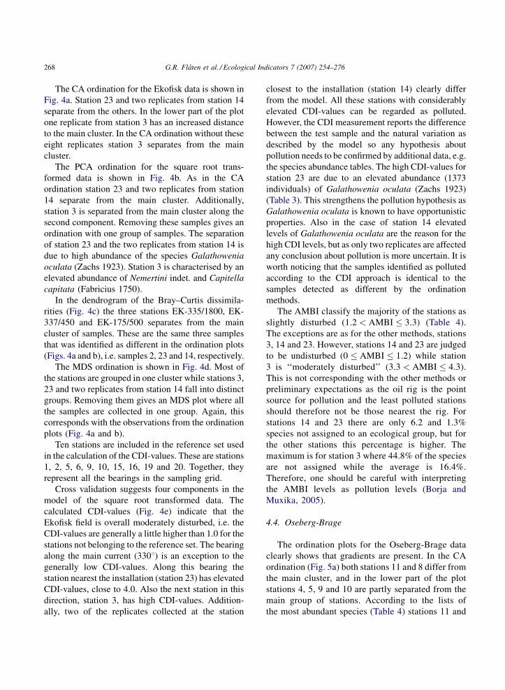
The CA ordination for the Ekofisk data is shown in

Fig. 4a. Station 23 and two replicates from station 14

separate from the others. In the lower part of the plot

one replicate from station 3 has an increased distance

to the main cluster. In the CA ordination without these

eight replicates station 3 separates from the main

cluster.

The PCA ordination for the square root trans-

formed data is shown in Fig. 4b. As in the CA

ordination station 23 and two replicates from station

14 separate from the main cluster. Additionally,

station 3 is separated from the main cluster along the

second component. Removing these samples gives an

ordination with one group of samples. The separation

of station 23 and the two replicates from station 14 is

due to high abundance of the species Galathowenia

oculata (Zachs 1923). Station 3 is characterised by an

elevated abundance of Nemertini indet. and Capitella

capitata (Fabricius 1750).

In the dendrogram of the Bray–Curtis dissimila-

rities (Fig. 4c) the three stations EK-335/1800, EK-

337/450 and EK-175/500 separates from the main

cluster of samples. These are the same three samples

that was identified as different in the ordination plots

(Figs. 4a and b), i.e. samples 2, 23 and 14, respectively.

The MDS ordination is shown in Fig. 4d. Most of

the stations are grouped in one cluster while stations 3,

23 and two replicates from station 14 fall into distinct

groups. Removing them gives an MDS plot where all

the samples are collected in one group. Again, this

corresponds with the observations from the ordination

plots (Fig. 4a and b).

Ten stations are included in the reference set used

in the calculation of the CDI-values. These are stations

1, 2, 5, 6, 9, 10, 15, 16, 19 and 20. Together, they

represent all the bearings in the sampling grid.

Cross validation suggests four components in the

model of the square root transformed data. The

calculated CDI-values (Fig. 4e) indicate that the

Ekofisk field is overall moderately disturbed, i.e. the

CDI-values are generally a little higher than 1.0 for the

stations not belonging to the reference set. The bearing

along the main current (3308) is an exception to the

generally low CDI-values. Along this bearing the

station nearest the installation (station 23) has elevated

CDI-values, close to 4.0. Also the next station in this

direction, station 3, has high CDI-values. Addition-

ally, two of the replicates collected at the station

closest to the installation (station 14) clearly differ

from the model. All these stations with considerably

elevated CDI-values can be regarded as polluted.

However, the CDI measurement reports the difference

between the test sample and the natural variation as

described by the model so any hypothesis about

pollution needs to be confirmed by additional data, e.g.

the species abundance tables. The high CDI-values for

station 23 are due to an elevated abundance (1373

individuals) of Galathowenia oculata (Zachs 1923)

(Table 3). This strengthens the pollution hypothesis as

Galathowenia oculata is known to have opportunistic

properties. Also in the case of station 14 elevated

levels of Galathowenia oculata are the reason for the

high CDI levels, but as only two replicates are affected

any conclusion about pollution is more uncertain. It is

worth noticing that the samples identified as polluted

according to the CDI approach is identical to the

samples detected as different by the ordination

methods.

The AMBI classify the majority of the stations as

slightly disturbed (1.2 < AMBI � 3.3) (Table 4).

The exceptions are as for the other methods, stations

3, 14 and 23. However, stations 14 and 23 are judged

to be undisturbed (0 � AMBI � 1.2) while station

3 is ‘‘moderately disturbed’’ (3.3 < AMBI � 4.3).

This is not corresponding with the other methods or

preliminary expectations as the oil rig is the point

source for pollution and the least polluted stations

should therefore not be those nearest the rig. For

stations 14 and 23 there are only 6.2 and 1.3%

species not assigned to an ecological group, but for

the other stations this percentage is higher. The

maximum is for station 3 where 44.8% of the species

are not assigned while the average is 16.4%.

Therefore, one should be careful with interpreting

the AMBI levels as pollution levels (Borja and

Muxika, 2005).

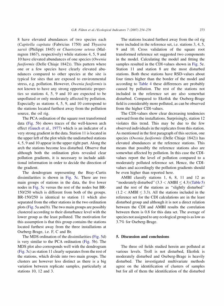
4.4. Oseberg-Brage

The ordination plots for the Oseberg-Brage data

clearly shows that gradients are present. In the CA

ordination (Fig. 5a) both stations 11 and 8 differ from

the main cluster, and in the lower part of the plot

stations 4, 5, 9 and 10 are partly separated from the

main group of stations. According to the lists of

the most abundant species (Table 4) stations 11 and


Fig. 4. The results obtained through the different multivariate analyses of the Ekofisk data. (a) The CA ordination plot for the Ekofisk data. The

numbers refer to the sampling site where the replicate is collected The replicates from station 23 and two replicates from station 14 separate, and

the analyses suggest that they are polluted. The rest of the samples assemble in one group. (b) The PCA ordination plot for the square root

transformed Ekofisk data. The numbers refer to the sampling site where the replicate is collected. As observed in the CA ordination the replicates

from station 23 and two replicates from station 14 separate. Additionally, station 3 separates along the second component. Subsequent analyses

show that station 3 is polluted. (c) The dendrogram of the Bray–Curtis dissimilarities calculated from the Ekofisk data. (d) MDS ordination of the

Bray–Curtis dissimilarities calculated from the Ekofisk data. The numbers refer to the sampling site where the replicate is collected. Exactly as in

the dendrogram stations 3, 23 and some replicates from station 14 separate. (e) The CDI-values calculated for the Ekofisk data. Shaded bars mark

the reference stations. The vertical line indicates CDI-values equal to 1.0, i.e. the border that separates disturbed and undisturbed stations. The

horizontal dashed lines separate the replicates from the different stations. The distance to the contamination source and the direction with regard

to the North is included for each sampling site.


Fig. 5. The results obtained through the different multivariate analyses of the Oseberg-Brage data. (a) The CA ordination plot for the Oseberg-

Brage data. The numbers refer to the sampling site where the replicate is collected. The replicates from stations 11 and 8 clearly separate, and the

further analyses prove that these stations are heavily polluted. (b) The PCA ordination plot for the square root transformed Oseberg-Brage data.

The numbers refer to the sampling site where the replicate is collected. As observed in the CA ordination the replicates from stations 11 and 8

clearly separate. (c) The dendrogram of the Bray–Curtis dissimilarities calculated from the Oseberg-Brage data. The three installations on the

field are indicated by F, C and BR. (d) MDS ordination of the Bray–Curtis dissimilarities calculated from the Oseberg-Brage data. The disturbed

stations are found in the upper part of the plot while the unpolluted samples (stations 3, 4, 5, 9, 10) are found in the lower part. (e) The CDI-values

calculated for the Oseberg-Brage data. Shaded bars mark the reference stations. The vertical line indicates CDI-values equal to 1.0, i.e. the border

that separates disturbed and undisturbed stations. The horizontal dashed lines separate the replicates from the different stations. The distance to

the contamination source and the direction with regard to the North is included for each sampling site. The CDI-values decrease along increasing

distance to the contamination source.


8 have elevated abundances of two species each

(Capitella capitata (Fabricius 1750) and Thyasira

sarsii (Philippi 1845) or Chaetozone setosa (Mal-

mgren 1867), respectively) while stations 4, 5, 9 and

10 have elevated abundances of one species (Owenia

fusiformis (Delle Chiaje 1842)). This pattern where

one or a few species have clearly elevated abu-

ndances compared to other species at the site is

typical for sites that are exposed to environmental

stress, e.g. pollution. However, Owenia fusiformis is

not known to have any strong opportunistic proper-

ties so stations 4, 5, 9 and 10 are expected to be

unpolluted or only moderately affected by pollution.

Especially as stations 4, 5, 9, and 10 correspond to

the stations located furthest away from the pollution

source, the oil rig.

The PCA ordination of the square root transformed

data (Fig. 5b) shows traces of the well-known arch

effect (Gauch et al., 1977) which is an indicator of a

very strong gradient in the data. Station 11 is located in

the upper left of the plot while the undisturbed stations

4, 5, 9 and 10 appear in the upper right part. Along the

arch the stations become less disturbed. Observe that

although both the ordination plots revealed clear

pollution gradients, it is necessary to include addi-

tional information in order to decide the direction of

the gradient.

The dendrogram representing the Bray–Curtis

dissimilarities is shown in Fig. 5c. There are two

main groups of stations in the data, the five lower

nodes in Fig. 5c versus the rest of the nodes but BR-

150/250 which is different from both of the groups.

BR-150/250 is identical to station 11 which also

separated from the other stations in the two ordination

plots (Fig. 5a and b). The two main groups are possibly

clustered according to their disturbance level with the

lower group as the least polluted. The motivation for

this assumption is that this group contains the stations

located furthest away from the three installations at

Oseberg-Brage, i.e. F, C and Br.

The MDS ordination of the dissimilarities (Fig. 5d)

is very similar to the PCA ordination (Fig. 5b). The

MDS plot also corresponds well with the dendrogram

(Fig. 5c) as station 11 clearly separates from the rest of

the stations, which divide into two main groups. The

clusters are however less distinct as there is a big

variation between replicate samples, particularly at

stations 10, 12 and 3.

The stations located furthest away from the oil rig

were included in the reference set, i.e. stations 3, 4, 5,

9 and 10. Cross validation of the square root

transformed reference set suggested two components

in the model. Calculating the model and fitting the

samples resulted in the CDI-values shown in Fig. 5e.

Station 11 and station 8 are the most disturbed

stations. Both these stations have RSD-values about

four times higher than the border of the model and

according to Table 4 these differences are probably

caused by pollution. The rest of the stations not

included in the reference set are also somewhat

disturbed. Compared to Ekofisk the Oseberg-Brage

field is considerably more polluted, as can be observed

from the higher CDI-values.

The CDI-values show clear decreasing tendencies

outward from the installations. Surprisingly, station 12

violates this trend. This may be due to the few

observed individuals in the replicates from this station.

As mentioned in the first paragraph of this section, one

species (Owenia fusiformis (Delle Chiaje 1842)) has

elevated abundances at the reference stations. This

means that possibly the reference stations also are

somewhat affected by pollution. In this case the CDI-

values report the level of pollution compared to a

moderately polluted reference set. Hence, the CDI-

values and accordingly the pollution gradients should

be even higher than reported here.

AMBI classify stations 1, 6, 8, 11 and 12 as

‘‘moderately disturbed’’ (3.3 < AMBI � 4.3) (Table 5)

and the rest of the stations as ‘‘slightly disturbed’’

(1.2 < AMBI � 3.3). All the stations included in the

reference set for the CDI calculations are in the least

disturbed group and although it is not a direct relation

between the CDI and AMBI results the correlation

between them is 0.8 for this data set. The average of

species not assigned to any ecological group is as low as

3.7% for Oseberg-Brage.

5. Discussion and conclusions

The three oil fields studied herein are polluted at

various levels. Troll is not disturbed, Ekofisk is

moderately disturbed and Oseberg-Brage is heavily

disturbed. The investigated multivariate methods

agree on the identification of clusters of samples

but for all of them the identification of the disturbed


samples relies on lists of species abundance. AMBI

has an additional requirement which is preliminary

assignment of the species to one of five ecological

groups. On the other hand, if an assigned species list

covering all the species in the sample is available

AMBI can provide a classification in accordance with

the Water Framework Directive (2000/60/EC)

directly. In this work the AMBI results from Troll

and Ekofisk must be carefully interpreted due to a high

percentage of species not assigned to any ecological

group. For Oseberg-Brage the percentage of not

assigned species were low, and this was also the data

set for which AMBI corresponded best with the other

multivariate methods including the CDI.

The multivariate methods differ in their level of

information. The methods based on the dissimilarity

matrix do not contain quantitative information. This is

obvious, since the Bray–Curtis dissimilarity is not a

Euclidean distance measurement (Borg and Groenen,

1997, p. 55). Although quantitative information is not

kept there are methods and dissimilarity measures

that can give biologically significant information

from dissimilarity measures (e.g. Clarke and War-

wick, 1994) but this is not further discussed here. In

the ordination plots the quantitative differences are

conserved and to some extent it is possible to extract

them visually. On the other hand, it is not obvious how

to report the quantitative information beyond pre-

senting the ordination plots. In modelling, the model

describes the natural variation and the samples are

compared to this model. The samples’ distances to the

model are a measurement of the difference to the

natural variation. Thus, the CDI-values, which

correspond to normalised distances, can be used as

a quantitative measurement of pollution in an area

with relatively homogenous natural variation. Sam-

ples with CDI-values lower than 1.0 are not disturbed

at the selected level of significance (Eq. (10)).

Samples which have CDI-values higher than 1.0

are disturbed and the size of the CDI-value

corresponds to the level of disturbance (pollution).

Thus, the list of CDI-values for the samples in a data

set gives a quantitative report of the level of pollution

at each station. Such a list makes it possible to

compare the pollution level in different surveys for a

field monitored several times, for instance. Another

application is ranking of relative pollution levels

among different fields which is difficult by means of

ordination methods and the qualitative dissimilarity

matrix methods.

It is not emphasised in this work, but the

modelling approach depends on selecting a good

reference set so as to avoid misleading CDI-values.

A good reference set gives a good representation of

the natural variation in the investigated area. The

consequence of a poor reference set is incorrect

border of the model, i.e. the calculated CDI-values

cannot be regarded as reliable pollution estimates.

The reference set is poor when too few stations are

included (the natural variation is not fully spanned)

and it is poor if too many, i.e. disturbed stations, are

included (the model becomes too wide). Combining

available information regarding the test area and the

ordinations is the evident way of selecting reference

stations. For the cases studied in this work typically

the outermost stations (those furthest away from the

pollution source) are included in the reference set.

Other constraints can be feasible if the CDI approach

is used in other applications.

AMBI is also a multivariate index that uses the

quantitative information in the abundance data as well

as the species identity. AMBI builds on previously

proposed ecological models (Borja et al., 2000) and a

preliminary classification of species in one of five

ecological groups. This can be difficult if a new region

is investigated, c.f. the high percentage of not assigned

species for Troll and Ekofisk. However, over time it

should be possible to build a species list covering any

region of interest. The challenge is though that in order

to assign a species to an ecological group a certain

level of knowledge about the species is required.

Hence, the two critical points in AMBI are (i) that the

underlying model is correct and valid for all regions

and (ii) that all species are and are correctly assigned

to an ecological group.

In the earlier mentioned Water Framework Direc-

tive (2000/60/EC) it is proposed to categorize water

quality in five classes. The scientists behind AMBI has

taken this into account and proposed how AMBI can

be used in classification in accordance with the

directive (Borja et al., 2004). No such work is done in

order to adapt the CDI to the EC’s water directive.

However, the authors believe that the modelling

approach should be well suited to meet the require-

ments in the directive. Particularly since the directive

relate all the pollution or disturbance levels to ‘‘normal


conditions’’. Thus, if the scientist is able to choose a

reference set that reflects the normal conditions, CDI

is a direct reflection of how different the ecological

status of stations is from these normal conditions.

Combining methods is the best approach to

analysis of benthic count data. Some kind of clustering

or ordination is a good start. If the ordination separates

any groups the tables of species abundances help to

distinguish polluted and undisturbed samples. The

undisturbed samples can be brought together in a

reference set, and subsequently a model of the natural

variation in the sampling area can be calculated from

this reference set. Comparing the samples to the

calculated model gives the CDI-values, which reports

quantitative information regarding the relative level of

disturbance in the monitoring area.

Even though the CDI approach is confined to

estimation of pollution levels in this work, it is

believed that the approach also can be useful in other

applications where it is of interest to quantify e.g.

differences in ecological status. The prerequisite is a

set of samples that define a reference area or state

which other samples can be compared to. Hence, the

different samples’ similarities to the pre-defined

reference state are calculated and various environ-

mental gradients can be quantified.

Acknowledgements

Norsk Hydro ASA and Phillips Petroleum Com-

pany Norway are thanked for giving access to their

data from the regular survey and monitor program of

the oil fields on the Norwegian shelf. The Norwegian

Research Council (NFR) is thanked for their financial

support to the project.

References

Borg, I., Groenen, P., 1997. Modern Multidimensional Scaling—

Theory and Applications. Springer, New York.

Borja, A., Franco, J., Perez, V., 2000. A marine biotic index to

establish the ecological quality of soft-bottom benthos within

European estuarine and coastal environments. Mar. Pollut. Bull.

40 (12), 1100–1114.

Borja, A., Franco, J., Muxika, I., 2004. The biotic indices and the

Water Framework Directive: the required consensus in the new

benthic monitoring tools. Mar. Pollut. Bull. 48, 405–408.

Borja, A., Muxika, I., 2005. Guidelines for the use of AMBI (AZTI’s

marine biotic index) in the assessment of the benthic ecological

quality. Mar. Pollut. Bull. 50, 787–789.

Bray, J.R., Curtis, J.T., 1957. An ordination of the upland forest

communities of southern Wisconsin. Ecol. Monogr. 27, 325–

349.

Clarke, K.R., 1990. Comparison of dominance curves. J. Exp. Mar.

Biol. Ecol. 138 (1–2), 130–143.

Clarke, K.R., Warwick, R.M., 1994. Change in Marine Commu-

nities: An Approach to Statistical Analysis and Interpretation.

Plymouth Marine Laboratory, UK.

Diaz, R.J., Solan, M., Valente, R.M., 2004. A review of approaches

for classifying benthic habitats and evaluating habitat quality. J.

Environ. Manage. 73, 165–181.

Everitt, B., 1980. Cluster Analysis, 2nd ed. Heinemann, London.

Flaten, G.R., 2002. Dynamic environmental monitoring by means of

multivariate modelling. Ph.D. Thesis. University of Bergen,

Norway.

Flaten, G.R., Grung, B., Kvalheim, O.M., 2004. A method for

validation of reference sets in SIMCA modelling. Chem. Intell.

Lab. Syst. 72, 101–109.

Gauch, H.G., Whittaker, R.H., Wentworth, T.R., 1977. A compara-

tive study of reciprocal averaging and other ordination techni-

ques. J. Ecol. 65, 157–174.

Gray, J.S., 2000. The measurement of marine species diversity, with

an application to the benthic fauna of the Norwegian continental

shelf. J. Exp. Mar. Biol. Ecol. 250, 23–49.

Hirschfeld, H.O., 1935. A connection between correlation and

contigency. Proc. Camb. Philos. Soc. 31, 520–524.

Hotelling, H., 1933. Analysis of a complex of statistical variables

into principal components. J. Educ. Psychol. 24 417–444 and

498–520.

Hurlbert, 1971. The nonconcept of species diversity—a critique and

alternative parameters. Ecology 52, 577–586.

Johnson, R.A., Wichern, D.W., 1992. Applied Multivariate Statis-

tical Analysis, 3rd ed. Prentice Hall, New Jersey.

Jongmann, R.H.G., Ter Braak, C.J.F., Van Tongeren, O.F.R., 1995.

Data Analysis in Community and Landscape Ecology. Cam-

bridge University Press, Cambridge, UK.

Kruskal, J.B., 1964. Multidimensional scaling by optimizing

goodness of fit to a nonmetric hypothesis. Psychometrika 29,

1–27.

Kvalheim, O.M., Brakstad, F., Liang, Y.-Z., 1994. Preprocessing of

analytical profiles in the presence of homoscedastic or hetero-

scedastic noise. Anal. Chem. 66 (1), 43–51.

Massart, B.G.J., 1997. Environmental monitoring and forecasting by

means of multivariate methods. Ph.D. Thesis. University of

Bergen, Norway.

Massart, B.G.J., Kvalheim, O.M., Libnau, F.O., Ugland, K.I.,

Tjessem, K., Bryne, K., 1996. Projective ordination by

SIMCA: a dynamic strategy for cost-efficient environmental

monitoring around offshore installations. Aquat. Sci. 58 (2),

120–138.

Olsgard, F., Gray, J.S., 1995. A comprehensive analysis of the effects

of offshore oil and gas exploration and production on the benthic

communities of the Norwegian continental shelf. Mar. Ecol.

Progr. Ser. 122, 277–306.


Pielou, E.C., 1966. The measurement of species diversity in differ-

ent types of biological collections. J. Theoret. Biol. 13, 131–144.

Rosenberg, D.M., Resh, V.H. (Eds.), 1993. Freshwater Bio-mon-

itoring and Benthic Macroinvertebrates. Chapman and Hall,

London.

Shannon, C.E., Weaver, W., 1949. The Mathematical Theory of

Communication. University of Illinois Press, Urbana.

Shepard, R.N., 1962. The analysis of proximities: multidimensional

scaling with an unknown distance function. Psychometrika 27,

125–140.

The Norwegian Pollution Control Authority (SFT), 1997. Guide-

lines for environmental monitoring of petroleum activities on the

Norwegian shelf, TA: 1424/1997.

Wold, S., 1976. Pattern recognition by means of disjoint principal

components models. Pattern Recogn. 8, 127–139.

Wold, S., 1978. Cross-validatory estimation of the number of

components in factor and principal components models. Tech-

nometrics 20, 397–405.

Wold, S., Esbensen, K., Geladi, P., 1987. Principal component

analysis. Chem. Intell. Lab. Syst. 2, 37–52.

Quantifying disturbances in benthic communities—comparison of the community disturbance index...

Documents

Transcript of Quantifying disturbances in benthic communities—comparison of the community disturbance index...