
Hidden disturbance in regional vegetation dynamics from road ...
287
HIDDEN DISTURBANCE IN REGIONAL VEGETATION DYNAMICS FROM ROAD PAVING IN A COUPLED NATURAL AND HUMAN SYSTEM: A CASE STUDY FROM THE SOUTHWEST AMAZON By GERALDINE KLARENBERG A DISSERTATION PRESENTED TO THE GRADUATE SCHOOL OF THE UNIVERSITY OF FLORIDA IN PARTIAL FULFILLMENT OF THE REQUIREMENTS FOR THE DEGREE OF DOCTOR OF PHILOSOPHY UNIVERSITY OF FLORIDA 2017
-
Upload
khangminh22 -
Category
Documents
-
view
3 -
download
0
Transcript of Hidden disturbance in regional vegetation dynamics from road ...

HIDDEN DISTURBANCE IN REGIONAL VEGETATION DYNAMICS FROM ROAD PAVING IN A COUPLED NATURAL AND HUMAN SYSTEM: A CASE STUDY FROM
THE SOUTHWEST AMAZON
By
GERALDINE KLARENBERG
A DISSERTATION PRESENTED TO THE GRADUATE SCHOOL OF THE UNIVERSITY OF FLORIDA IN PARTIAL FULFILLMENT
OF THE REQUIREMENTS FOR THE DEGREE OF DOCTOR OF PHILOSOPHY
UNIVERSITY OF FLORIDA
2017

© 2017 Geraldine Klarenberg

To my children and my parents

4
ACKNOWLEDGMENTS
I would like to thank my advisor, Dr Rafael Muñoz-Carpena for his unwavering
support throughout the years. His enthusiasm for science, passion for learning new
things and his willingness to discuss ideas and methods have been invaluable to my
development as a scientist.
I would also like to thank my Co-Chair Dr. Greg Kiker and my committee, Dr.
Stephen Perz, Dr. Wendell Cropper and Dr. Mark Brown for their guidance and
feedback. I am grateful for the time they have made available to provide support and
input into this research. The diversity of their viewpoints and backgrounds have been
important in increasing my understanding of various disciplines.
I am indebted to the National Science Foundation for the funding provided for the
first part of my research.
From the UF Department of Agricultural and Biological Engineering, I am grateful
to Dr. Ray Huffaker, Dr. Miguel Campo-Bescos, Dr. Matteo Convertino, Dr. Galia
Selaya, Miles Medina, and from the UF Department of Geography Dr. Jane Southworth,
Dr. Matt Marsik, Dr. Erin Bunting and Dr. Likai Zhu. Without their help with data
collection, guidance on methods and discussions on topics of interest, this study would
have surely not come to be.
Staff at the UF High Performance Computing Center, specifically Matt
Gitzendanner, Max Prokopenko, Alex Moskalenko and Ying Zhang, have been
tremendously helpful and I thank them for all their assistance.
There are so many friends who took this journey with me; some on the same
journey, others on a completely different path, but always understanding and caring.
Everyone’s kind words and encouragement have buoyed me these past years.

5
Last but not least I would like to thank my family from the bottom of my heart.
First and foremost, my kids Sebastiaan and Amara, who never asked for their mom to
do a PhD, but who had to deal with my absences, long work hours and forgetfulness.
They put up with it, loved me more than anything anyway and were my indefatigable
cheerleaders during that last push to finish. My husband Chris and his kids Charlotte
and Jack, for the love, support and understanding during these long years. Chris’
support was invaluable, as he provided a listening ear (for both my excitement as well
as my griping), helped me with computer problems, always kept me grounded, and
gave me a place of love to come home to every day. Finally, my parents Richard and
Marga – they raised me to have grit and to believe in myself. Without those two things,
this dissertation would not have come to fruition. While far away, they are always in my
thoughts and my heart. We have had to miss each other for too long and I am looking
forward to more visits home.

6
TABLE OF CONTENTS page
ACKNOWLEDGMENTS ...................................................................................................... 4
LIST OF TABLES ................................................................................................................ 9
LIST OF FIGURES ............................................................................................................ 11
LIST OF ABBREVIATIONS ............................................................................................... 13
ABSTRACT ........................................................................................................................ 15
CHAPTER
1 INTRODUCTION ........................................................................................................ 17
Coupled Human Natural Systems, Complexity and Change..................................... 17 Stability, Regime Shifts and Resilience ............................................................... 18 Road Infrastructure Development and Forest Degradation ................................ 20 Ecosystem Services and Ecosystem Function ................................................... 21 Ecosystem Function and Vegetation Dynamics .................................................. 23 The Study Area .................................................................................................... 25
Hypothesis and Sub-Hypotheses ............................................................................... 31 Hypothesis ............................................................................................................ 31 Expected Significance .......................................................................................... 31 Sub-Hypotheses ................................................................................................... 32
2 A SPATIAL-TEMPORAL DATABASE TO EVALUATE ROAD DEVELOPMENT IMPACTS IN A COUPLED NATURAL-HUMAN SYSTEM IN A TRI-NATIONAL FRONTIER IN THE AMAZON .................................................................................... 41
Background and Summary ......................................................................................... 41 Methods ....................................................................................................................... 44
Data Collection and Compilation ......................................................................... 44 Human Variables .................................................................................................. 44 Environmental Variables ...................................................................................... 47 Stationary Variables ............................................................................................. 53
Data Records .............................................................................................................. 56 Technical Validation ............................................................................................. 57 Usage Notes ......................................................................................................... 59
3 CLUSTER ANALYSIS OF VEGETATION DYNAMICS AND ASSOCIATION WITH ROAD PAVING ................................................................................................. 65
Background ................................................................................................................. 65 Methods ....................................................................................................................... 68

7
Data ...................................................................................................................... 68 Time Series Clustering Based on an Adaptive Dissimilarity Index ..................... 69 Clustering Validation Measures ........................................................................... 71 Number of States and Breakpoint Analysis ......................................................... 73 Data Availability .................................................................................................... 74
Results ........................................................................................................................ 74 Four EVI2 Clusters Along a Road Paving Gradient ............................................ 74 Additional Cluster Analysis on Biophysical Variables ......................................... 75 States and Breakpoint Analysis ........................................................................... 76
Discussion ................................................................................................................... 76 Assessment of Final Clusters .............................................................................. 76 Comparison of States Changes ........................................................................... 77 Methodological Findings: Cluster Selection and State Changes ........................ 78
4 CHANGING LANES: HIGHWAY PAVING IN THE SOUTHWESTERN AMAZON ALTERS LONG-TERM TRENDS AND DRIVERS OF REGIONAL VEGETATION DYNAMICS ........................................................................................ 88
Background ................................................................................................................. 88 Results ........................................................................................................................ 93
Identification of Clusters Vegetation Dynamics and their Association with Road Paving Extent .......................................................................................... 93
Common Trends Explain the Shared Variability of Each VDC ........................... 94 In a Disturbed System State, Covariates Explain More of the Variance In
Vegetation Dynamics Than in an Undisturbed System State.......................... 95 Variables Associated with Anthropogenic Activity Increase in Importance in
Explaining Vegetation Dynamics in the Disturbed System State .................... 96 Among Natural Covariates, Temperature is the Main Direct Driver of
Vegetation Dynamics ........................................................................................ 98 Low Frequency Signals Explain Trend Behavior Across the Study Area as a
Whole, but Dominate Particularly in the Paved State ....................................101 Unpaved to Paved Conditions Represent Two Stable System States with a
Transition State in Between Them .................................................................103 Discussion .................................................................................................................104
Main Findings .....................................................................................................104 Broader Impacts .................................................................................................105 Limitations and Further Research .....................................................................106
Methods .....................................................................................................................107 Study Area ..........................................................................................................107 Response Covariate: Vegetation Dynamics, EVI2 ............................................108 Candidate Covariates Related to Human Activity .............................................109 Candidate Covariates Associated with Biophysical Processes ........................110 Clustering ...........................................................................................................111 Lagging and Reduction of Covariate Data Set ..................................................112 Dynamic Factor Analysis ...................................................................................113 Importance of Trends and Covariates ...............................................................114 Spectral Analysis of Trends ...............................................................................115

8
Software Used ....................................................................................................115 Data Availability ..................................................................................................116
5 CAUSALITY ANALYSIS OF REGIONAL BIOPHYSICAL AND VEGETATION VARIABLES REVEALS INCREASED FEEDBACK ALONG A ROAD PAVING GRADIENT IN THE SW AMAZON ...........................................................................128
Background ...............................................................................................................128 Materials and Methods .............................................................................................135
Study Site and Data ...........................................................................................135 Methods ..............................................................................................................138 Data Availability ..................................................................................................145
Results ......................................................................................................................145 Identification of Four Vegetation Dynamics Clusters along a Road Paving
Gradient ...........................................................................................................145 Signal separation reveals different signals for vegetation in each VDC...........146 Causality testing of signals for three VDCs indicates an increase in causal
relationships for EVI ........................................................................................148 Discussion .................................................................................................................150
Vegetation Dynamics Clusters and Signals ......................................................150 Application of Causality Analyses on Complex Systems: Implications of
Findings and Methods ....................................................................................151 Concluding Remarks ................................................................................................155
6 CONCLUSIONS ........................................................................................................169
Main Findings ............................................................................................................169 Scientific Findings ..............................................................................................169 Methodological Findings ....................................................................................176
Limitations And Future Research .............................................................................177 Broader Impacts ........................................................................................................181
APPENDIX
A SUPPLEMENTARY MATERIALS FOR CHAPTER 4 ..............................................184
B SUPPLEMENTARY MATERIALS FOR CHAPTER 5 ..............................................212
C ADDITIONAL NOTES ON GRANGER CAUSALITY ANALYSIS ............................243
Granger Prediction ....................................................................................................243 Results for Granger Prediction .................................................................................245 Discussion .................................................................................................................246
LIST OF REFERENCES .................................................................................................266
BIOGRAPHICAL SKETCH ..............................................................................................287

9
LIST OF TABLES
Table page 2-1 Overview of dynamic variables collected and compiled for the area in Madre
de Dios (Peru), Acre (Brazil) and Pando (Bolivia), the MAP area. ....................... 60
2-2 Overview of stationary data collected and compiled for the area in Madre de Dios (Peru), Acre (Brazil) and Pando (Bolivia), the MAP area. ............................ 63
3-1 Dunn Index and Silhouette Width results from all clustering options for EVI2 ..... 79
3-2 Values of the validation measures indicating the best number of VDCs after a hierarchical cluster analysis. .................................................................................. 80
4-1 List of variables used in the analysis, their unit of measure, and source. ..........117
4-2 Results of dynamic factor analyses of Enhanced Vegetation Index (EVI2) for 4 Vegetation Dynamics Areas (VDCs).................................................................119
5-1 Periodicities that were selected to create reconstructed signals of time series and the contribution of each signal to the decomposition ...................................157
5-2 Surrogate data test results ...................................................................................160
5-3 Significant cross skill mapping after applying extended CCM ............................163
A-1 Overview of communities included in the study. .................................................184
A-2 Statistical characteristics of monthly EVI2 time series (1982 – 2010) per VDC .187
A-3 Statistical properties of the monthly area-weighted time series of Candidate Explanatory Variables ..........................................................................................188
A-4 Lags applied to time series of candidate explanatory variables. ........................190
A-5 Results of Variation Inflation Factor (VIF) analysis for explanatory variables included in dynamic factor analyses per VDC. ....................................................191
A-6 Dynamic Factor Model (Model I, trends only) goodness-of-fit results of selected (best) models for individual communities. .............................................192
A-7 Average relative importance of trends and explanatory variables in dynamic factor analyses (Model II, trends and explanatory variables) simulating EVI2 ...195
A-8 Dynamic Factor Model (Model II, trends and explanatory variables) goodness-of-fit results of selected (best) models for individual communities. ...199
10
A-9 Beta coefficients (weightings, β) of the explanatory variables for the selected Dynamic Factor Models II (trends and explanatory variables)............................202
A-10 Factor loadings (weightings, α) of the trends for the selected Dynamic Factor Models II (trends and explanatory variables), for each community. ...................206
A-11 Frequencies, cycle lengths and spectral power density values for the Pacific Decadal Oscillation (PDO) ...................................................................................210
B-1 Cycle lengths (months) used to set the window length in Singular Spectrum Analysis (based on spectral density results). ......................................................212
B-2 Weighted adjacency matrices ..............................................................................213
B-3 Relevant lags identified with extended CCM .......................................................214
C-1 Results of Granger causality analysis for VDC 4 ................................................247
C-2 VAR models with p value for the Ljung-Box test > 0.05 ......................................248
C-3 Granger causality test results for all variables (at selected AR order) ...............256

11
LIST OF FIGURES
Figure page 1-1 Schematic representation of the relationships between ecosystem services
and functions, and the human system, including the role of vegetation dynamics. ................................................................................................................ 39
1-2 The MAP area in Peru, Brazil and Bolivia, with the Inter Oceanic Highway, other roads, protected areas major cities and communities ................................. 40
2-1 Comparison of monthly values per community polygon for AVHRR-derived EVI (1982-1999) and “true” EVI (2000-2010) ........................................................ 64
3-1 Average values of EVI2 and biophysical variables per community for the period 1987-2009 ................................................................................................... 81
3-2 Analysis framework for clustering analysis ............................................................ 83
3-3 Selection criteria for determination of the appropriate number of clusters ........... 84
3-4 Dendrogram of EVI2 time series clusters, with 4 clusters selected. ..................... 85
3-5 Characteristics of the study area ........................................................................... 86
4-1 Characteristics of the study area after clustering analysis ..................................121
4-2 Contributions of model components of the final VDC DFMs II for each community to explaining variance in vegetation dynamics .................................122
4-3 Proportion of variance explained by each covariate for each community ..........123
4-4 Lagged time series of the covariates used in the final Dynamic Factor Models (DFMs) II for each VDC ........................................................................................124
4-5 𝛽 coefficients of the covariates used in the final Dynamic Factor Models
(DFMs) II for each VDC ........................................................................................125
4-6 Characteristics of the trends (unknown explained variance) in the selected Dynamic Factor Models II ....................................................................................126
4-7 Flow chart of methods ..........................................................................................127
5-1 Analysis framework for causality analysis ...........................................................164
5-2 Characteristics of the study area after clustering analysis. .................................165
5-3 Reconstructed time series, the signals, after Singular Spectrum Analysis ........166

12
5-4 Heat maps for the observed EVI2, reconstructed EVI2, and line plots for the observed and reconstructed EVI2........................................................................167
5-5 Networks of cross-mapping skill (𝜌) of deterministic signals of EVI (𝜌 ≥ 0.65)
per VDC, after testing for false positives due to synchronicity ............................168
A-1 Simulated and observed monthly Enhanced Vegetation Index (EVI2) time series ....................................................................................................................211
B-1 Observed, area-weighted time series for each VDC ...........................................216
B-2 Results of Singular Value Decomposition (VDC) of time series of VDC 1 .........217
B-3 Results of Singular Value Decomposition (VDC) of time series of VDC 2 .........221
B-4 Results of Singular Value Decomposition (VDC) of time series of VDC 3 .........225
B-5 Results of Singular Value Decomposition (VDC) of time series of VDC 4 .........229
B-6 Results of Singular Value Decomposition (VDC) of time series of climate indices ...................................................................................................................233
B-7 Lineplots and heatmaps of original and reconstructed time series of all variables for all 4 VDCs ........................................................................................234
B-8 Nonlinear cross-prediction skill to determine stationarity of signals, per VDC ...241
B-9 Networks of cross-mapping skill (𝜌) of deterministic signals (𝜌 ≥ 0.65) per VDC, after testing for false positives due to synchronicity ..................................242
C-1 Conditional Granger causality (p<0.05) results for VDC 1 and VDC 4 ...............265

13
LIST OF ABBREVIATIONS
AAFT Amplitude Adjusted Fourier Transform
AIC Akaike’s information Criterion
AMO Atlantic Multidecadal Oscillation
AVHRR Advanced Very High Resolution Radiometer
BEF Biodiversity-Ecosystem Functioning
BIC Bayesian Information Criterion
CCM Convergent Cross Mapping
CNH Coupled Natural Human
CPC Climate Prediction Center (NOAA)
CRU Climate Research Center (University of East Anglia)
DBH Diameter at breast height
DEM Digital Elevation Map
DFA Dynamic Factor Analysis
DFM Dynamic Factor Model
ENSO El Niño / Southern Oscillation
EVI Enhanced Vegetation Index
EVI2 Enhanced Vegetation Index 2
fPAR Fraction of Photosynthetically Active Radiation
GC Granger Causality
IIRSA Initiative for the Integration of the Regional Infrastructure of South America
IOH Inter-Oceanic Highway
IQR Interquartile Range
LAI Leaf Area Index

14
MAP Madre de Dios / Acre / Pando
MASL Meters above sea level
MEI Multivariate ENSO Index
MODIS Moderate Resolution Imaging Spectroradiometer
NDVI Normalized Difference Vegetation Index
NFTP Non-Forest Timber Product
NOAA National Oceanic and Atmospheric Administration
NPP Net primary Production
NSE Nash-Sutcliffe Coefficient of Efficiency
PDO Pacific Decadal Oscillation
PET Potential Evapotranspiration
PFT Plant Functional Type
PPS Pseudo Phase Space
SSA Singular Spectrum Analysis
SVD Singular Value Decomposition
UN-REDD United Nations Programme on Reducing Emissions from Deforestation and Forest Degradation
VDC Vegetation Dynamics Cluster
VIF Variance Inflation Factor
VIP Vegetation Index and Phenology (research group at the University of Arizona)

15
Abstract of Dissertation Presented to the Graduate School of the University of Florida in Partial Fulfillment of the Requirements for the Degree of Doctor of Philosophy
HIDDEN DISTURBANCE IN REGIONAL VEGETATION DYNAMICS FROM ROAD
PAVING IN A COUPLED NATURAL AND HUMAN SYSTEM: A CASE STUDY FROM THE SOUTHWEST AMAZON
By
Geraldine Klarenberg
December 2017
Chair: Rafael Muñoz-Carpena Cochair: Greg Kiker Major: Agricultural and Biological Engineering
Infrastructure development, specifically road construction, contributes socio-
economic benefits to society worldwide. However, detrimental environmental effects of
road construction have been documented, most notably increased deforestation.
Beyond deforestation, this study hypothesized that road construction introduces
degradation, “unseen” regional effects on forests, over time. This potentially leads to
changes in ecosystem services a forest provides. In coupled natural-human (CNH)
systems this has implications for both nature and humans. At a regional scale, such
changes would be visible in vegetation dynamics: as species composition shifts or
vegetation structure changes, the phenology patterns, or vegetation dynamics, change.
To test this hypothesis, we use a long-term remotely sensed vegetation index,
EVI2, as a proxy for vegetation dynamics, combined with field-based socio-ecological
data and biophysical data from global data sets, for a transboundary region in the
southwestern Amazon that has been subject to construction of the Inter-Oceanic
Highway (IOH) during our study period of (1987–2009). These data were available for
99 communities that experienced road paving at different times. Specialized time series

16
analysis techniques were applied, designed to uncover underlying structure of
vegetation dynamics and find linkages with other localized variables. First, we found 4
areas of common vegetation dynamics associated with the average extent of road
construction, Vegetation Dynamics Clusters (VDCs). We analyzed the importance of
shared trends and explanatory variables within and across VDCs with a multivariate
time series reduction technique, Dynamic Factor Analysis. We found that human-related
covariates become more important in explaining forest structure dynamics as road
construction intensity increases. Trends, indicators of underlying unexplained effects,
become relatively less important as construction increases and are dominated by lower
frequency signals; potentially influenced by climate indices. By applying novel causality
analyses, we identified increased feedback in causal relationships from vegetation
dynamics to biophysical variables from the unpaved to the paved state. This potentially
indicates less stability, and more opportunity for vegetation changes to affect the local
and global climate. This study indicates the need for a focus on regional degradation as
part of road infrastructure development projects in forest-rich countries.

17
CHAPTER 1 INTRODUCTION
Coupled Human Natural Systems, Complexity and Change
Coupled natural and human (CNH) systems are defined as “integrated systems
in which people interact with natural components” (J. Liu et al., 2007). Further than that
though, it provides a framework for scientific understanding in which processes and
complex interactions between human and natural systems are integrated (Chen and Y.
Liu, 2014). Dynamics in one system affect dynamics in the other, and when changes
occur in one, this is often carried over to the other in a nonlinear fashion. As many
natural and human systems become more interwoven due to increased exploitation,
expansion of human living space, increased population and climate change, research
on understanding these systems is important. Gaining insight into issues of ecological
deterioration and sustainable development are paramount, and researching only one or
the other system will be unlikely to paint a complete picture of the challenges and
potential solutions. As Liu et al. (2007) point out, many systems are unique and will
need unique research and solutions. All of them have characteristics of complex
systems though: feedback loops, nonlinear dynamics, thresholds, time lags,
heterogeneity, legacy effects, emergent properties (‘surprises’) and scale issues. In
essence, this can be summarized as spatial, temporal and organizational complexity
(Pickett et al., 2005). Spatial complexity refers to spatial heterogeneity and
configurations of components of the system. Temporal complexity considers the effects
of past states and legacies, and organizational complexity encompasses connectivity
between components. Emergent properties are an important aspect of understanding
complex systems: they refer to properties that emerge as a result of complex

18
interaction, i.e. they are not based on linear relationships and thus not easily predicted.
When researching change in complex systems, it becomes important to define change,
stability and (especially) resilience in the context of the system under consideration.
Stability, Regime Shifts and Resilience
It has been posited that systems can be subject to critical transitions, which
involves a drastic change of one state to another, due to a small change in a variable or
a small stochastic disturbance. This otherwise insignificant event causes a shift in
system state because the system has become increasingly fragile due to various earlier
disturbances (Gunderson and Holling, 2002; Hirota et al., 2011; Scheffer, 2009;
Scheffer et al., 2009; 2001). This current thinking has evolved from classical
catastrophe theory (Zeeman, 1976), a branch of bifurcation theory which particularly
regards hysteresis (a fold catastrophe) and cusp bifurcations (Scheffer et al., 2001).
Hysteresis occurs in situations where the value of a physical property lags behind
changes in the effect causing it. An example is algae outbreaks in surface water caused
by high nutrient loads; there is usually a particular value of nutrient loading at which the
system shifts from clear to an algae outbreak. However, to return the system to its
original clear state, nutrient loads need to be reduced far lower than the value at which
the system shifted in the first place. So, besides the catastrophical shift itself in the
system, it is also more difficult to return to the original system. Zeeman (1976) provided
applied examples of catastrophe theory in biology and behavioral sciences, and
applications of the theory and identification of phenomena such as multimodality (the
existence of multiple stable states, associated with hysteresis) have since expanded to
ecology (Frelich and Reich, 1999; Gunderson and Holling, 2002; Scheffer et al., 2001;
Wissel, 1984).

19
Importantly, Scheffer (2009) points out that it is simplistic to refer to “equilibria” or
“stable states” in complex and dynamic systems such as ecosystems or CNH systems,
and rather proposes the terms ‘regime’ and ‘regime shifts’. This terminology makes it
clear that a stable system is not necessarily in only one state: cyclical, chaotic and
oscillating systems can also be ‘stable’ since the regime in which the system cycles or
oscillates, or the (strange) attractor around or toward which it moves, are stable. This
complicates the identification of alternative stable regimes or change points; and in
addition, ecological systems generally display an amount of noise due to stochastic
events and processes.
‘Resilience’, as defined in the context of regime shifts (in chaotic and/or cyclical
systems), refers to the size of the ‘basin of attraction’ (Holling, 1973; Scheffer et al.,
2001), that is, the boundary of the area of the domain of an attractor. It is hypothesized
that this domain changes over time due to hysteresis. If a basin of attraction has been
identified and delineated for the identity of a particular system, the most pressing
question for practical purposes is where the system is positioned within the basin of
attraction at a particular point in time. If it is close to the edge, the outer boundary, less
change or disturbance is required to cause a regime shift, a critical transition.
A more practical and generally accepted description of ‘resilience’ is “the
persistence of relationships within a system and [it] is a measure of the ability of these
systems to absorb changes of state variables, driving variables, and parameters, and
still persist” (Holling, 1973). This description has been further refined by Cumming et al.
(2005), who note that relationships within a system often change, but in order for a
system to be resilient, “the essential attributes that define its identity must be

20
maintained”. It is therefore important to define the system under consideration; its
identity, and the attributes that define it.
Recent studies have indicated that the Amazon system in general is possibly
heading for a transition to a regime dominated by disturbances, with associated
changes in water and energy cycles (Davidson et al., 2012) or even that the system is
headed for a ‘critical transition’ or ‘tipping point’ related to deforestation and biome
changes (Nepstad et al., 2008; Nobre and Borma, 2009). Numerous studies have
simulated land cover changes taking place in the Amazon due to human-induced
climate change, anthropogenic disturbances and positive feedback cycles (Almeyda
Zambrano et al., 2010; Keller, 2009; Marsik et al., 2011).
Road Infrastructure Development and Forest Degradation
For forest ecosystems, road construction and paving are the main drivers of
deforestation (Laurance et al., 2002a; Marsik et al., 2011). There are also signs that
road paving contributes to degradation of forest systems. Previous research found that
even limited logging disturbances had a permanent local effect on forest structure in
Madagascar (Brown and Gurevitch, 2004). Differences in vegetation structure and
phenology between natural and anthropogenic treefall gaps 1 to 4 years after logging
were also identified in a Bolivian forest, despite almost identical forest cover
percentages (mean 88% for the anthropogenic gaps, and 91% for the natural gaps),
with lower mean number of flowering and fruiting plants in anthropogenic gaps, as well
as more regeneration of non-commercial pioneer species in these gaps (Felton et al.,
2006). A review study concluded that in Neotropical secondary forests, the recovery
trajectory of vegetation and its characteristics is uncertain in anthropogenic settings,
and dependent on site-specific factors and land use (Guariguata and Ostertag, 2001).

21
Changes in forest structure will in turn impact components of the system: changes in
tropical forest structure have been linked to modifications in wildlife populations in
Panama (DeWalt et al., 2003), and ecosystem productivity was found to be driven by
canopy phenology in the Amazon (Restrepo-Coupe et al., 2013). A forest inventory
study (Baraloto et al., 2015) found differences in forest value (based on biodiversity,
carbon stocks and timber and non-timber forest products), and highlighted that
deforestation and degradation do not always respond similarly to road paving.
Considering these findings and the need for better understanding of CNH systems,
there is a need to do more research on the complexity of road paving and forest
degradation. Road paving increases connectivity within an area and a CNH system,
making it important that research considers this issue regionally.
For research purposes, forest degradation needs a clearer meaning than this
broad collection of processes and changes. In this study, the definition of Putz and
Redford (2010) is adopted: “forests that lose their defining attributes (e.g., ancient trees,
fauna, and coarse woody debris) through logging, market hunting, wildfires, or invasion
by exotic species, become degraded forest”. This is in line with the earlier definition of
resilience and allows us to consider degradation in an comprehensive and systematic
manner. To streamline the approach further, ecosystem services can be considered as
one of these attributes, especially for CNH systems.
Ecosystem Services and Ecosystem Function
It has long been acknowledged in both science and society that nature provides
essential services, goods and cultural services to humankind – “ecosystem services”. In
the past, the focus has mainly been on tangible or direct benefits, such as materials
(wood, water); but more recently the scope has broadened to include “provisioning”,

22
“regulating”, “cultural” and “supporting” ecosystem services, as defined in the
Millennium Ecosystem Assessment (2005). The latter was initiated in 2001 with support
of the United Nations and overseen by a multistakeholder board, and “set out to assess
the consequences of ecosystem change for human well-being and to establish the
scientific basis for actions needed to enhance the conservation and sustainable use of
ecosystems and their contributions to human well-being.” The Millennium Ecosystem
Assessment gives a (non-exhaustive) list of various services that fall under the 4 earlier
mentioned categories of ecosystem services. Using this broad approach, the ecosystem
services of the Amazon as a whole have been found to be under great pressure (Foley
et al., 2007). Also at smaller scales, since CNH systems consist of ecological as well as
anthropogenic components and influences, it is reasonable to evaluate a system from
the point of view of ecosystem services. Then, in order to evaluate CNH systems in
terms of resilience and, possibly, tipping points, a decision needs to be made what
“identity” of the system to consider. For this research, we propose that vegetation
dynamics and structure are suitable when considering forest degradation due to their
linkages with ecosystem services (Figure 1-1). This will be explained in the following
sections.
The concept of ecosystem services is generally regarded as a subjective metric
since what is regarded as a service by one might not necessarily constitute as a service
for another. “Ecosystem services” implies some form of valuation, which is hardly ever
straightforward and hinders measurability. Instead, the associated notion of ecosystem
function is more objective and more measurable. Ecosystem functions are defined as
“the capacity of natural processes and components to provide goods and services that

23
satisfy human needs, directly or indirectly” (De Groot et al., 2002). Hence, services are
obtained from functioning of the ecosystem (Baraloto et al., 2014). Three generally
recognized ecosystem functions are the carbon, the hydrological and the nutrient cycle.
Each ecosystem function is a product of the natural processes that define its ecological
structure and processes, and the natural processes are a result of interactions of biotic
and abiotic components of the system (Figure 1-1). This is in line with the definition of
ecosystem functioning: “the rate, level or temporal dynamics of one or more ecosystem
processes such as primary production, total plant biomass, or nutrient, gain, loss, or
concentration” (Tilman, 2001).
Ecosystem Function and Vegetation Dynamics
Ecosystem functions that are of importance in forest areas in general are carbon
storage, and diversity. Specific species can provide very specific and local ecosystem
services (such as timber or non-timber products), whereas carbon storage provides a
more regional and global ecosystem service. The regional and global relevance in
diversity lies mostly in functional diversity (diversity of traits), which in turn supports
other functions and services such as carbon storage, hydrology and nitrogen cycles.
Forests that experience a reduction in their functioning (and thus services), while still
classified as a forest, can be regarded as a degraded forest, or a forest of lesser quality,
from an ecosystem services point-of-view.
The proposal to evaluate vegetation dynamics to assess forest degradation in a
CNH system stems from the notion that vegetation dynamics drive ecosystem
functioning, which in turn drives ecosystem services. Vegetation dynamics, also termed
phenology, play an important role in timing of ecosystem functions such the water and
carbon cycle, or primary productivity. Phenology – e.g. growth and senescence - is

24
affected by biophysical variables such as temperature and precipitation, and has been
used extensively to evaluate impacts of climate change (Donnelly and Yu, 2017; Menzel
et al., 2006). However, it also differs per species, so phenological signatures are also an
expression of species composition or vegetation structure. Recent controlled
experiments on the timing of flowering showed that increases or decreases in diversity
changed the timing of flowering (Wolf et al., 2017). Hence, different phenology patterns
or vegetation dynamics can imply differences in species composition, vegetation
structure or diversity. Vegetation dynamics are unique and a change in these dynamics
implies a change in vegetation structure and species composition, as well as a change
in subsequent ecosystem functions and services.
To analyze vegetation dynamics at a regional level and a longer time period, time
series of vegetation indices can be used. These remote sensing products have been
used in many studies to monitor and evaluate phenology (Asner et al., 2000; Morton et
al., 2014; Reed et al., 1994). The Enhanced Vegetation Index (EVI) is one of these
products. It is calculated from surface reflectances measured by the Moderate
Resolution Imaging Spectroradiometer (MODIS) satellite in a way that it reduces the
influence of aerosols and soil back scatter and decouples these influences from the
vegetation signal (Huete et al., 2010). The advantage of EVI over other indexes such as
the Normalized Difference Vegetation Index (NDVI) is its increased sensitivity in areas
with high biomass, i.e. it does not saturate at high values (Weng, 2011). Since EVI is a
measure of the contrast between absorption of blue and red wavelengths (by
chlorophyll in leaves) and scatter of near-infrared radiation (dependent on canopy
properties such as Leaf Area Index (LAI), leaf angle distribution, leaf morphology), it is

25
an expression of physiological and structural properties of the canopy (Huete et al.,
2010). It is sometimes also referred to as ‘greenness’: “the composite optical property of
canopy chlorophyll content, leaf area, vegetation cover, and structures” (Huete et al.,
2002). Though it does not give exact information in terms of species composition, it can
provide indications of structural change in a forest. The relationships between EVI and
biophysical vegetation properties such as Leaf Area Index (LAI), biomass or Gross
Primary Production and chlorophyll content, or “greenness” (through fPAR, fraction
absorbed photosynthetically active radiation) have been summarized in previous work
(Huete et al., 2002). The link with fPAR, or chlorophyll content, is clearest, as is the link
with gross primary production (though the latter was only established for temperate
regions (Huete et al., 2010).
The Study Area
This study focuses on the construction of the Inter-Oceanic Highway (IOH),
which connects ports on the Pacific coast of Peru with the Atlantic ports in Southern
Brazil, and runs through the so-called MAP area. The “MAP” area in the Southwestern
Amazon covers an area where three nations meet: Peru, Bolivia and Brazil (Figure 1-1).
The acronym MAP refers to the departments of these three countries that comprise the
area: Madre de Dios (Peru), Acre (Brazil) and Pando (Bolivia). The area lies between
9°48’ S and 13°1’ S latitude and 67°10’ and 70°31’ W longitude, at the foot of the Andes
Mountains and in the headwaters of the Amazon River. The climate is tropical, classified
as Awi (Köppen) with an average daily temperature of 25 °C and mean annual
precipitation of approximately 2000 mm. The dry season runs from June to September,
in which monthly rainfall averages < 100 mm (Marsik et al., 2011).

26
The types of forest in the area are dense tropical forest, open tropical forest with
palm trees, and open forests dominated by bamboo – with many locations containing a
mix of these forest types (Carvalho et al., 2013; Rockwell et al., 2014; Salimon et al.,
2011). The area is of significance for tropical conservation (Killeen and Solorzano,
2008; Myers et al., 2000; Phillips et al., 2006), with high diversity in biota in terms of tree
species, birds and insects (Phillips et al., 2006). The large Chico Mendes Extractive
Reserve forms part of the study area (in Brazil), as well as the Manuripi National Wildlife
Reserve (in Bolivia), Figure 1-2. The natural vegetation generally has a faster turnover
than forests further north and east; on average the western Amazon has a turnover rate
of 2.6% a-1 as opposed to 1.4% a-1 (Quesada et al., 2012), which is attributed to both
soil fertility and climate. Above ground biomass and stand-level wood density are also
lower in the region compared to the rest of the Amazon (Nogueira et al., 2008; Quesada
et al., 2012). Quesada et al. (2012) posit that feedback mechanisms associated with soil
physical quality is primarily responsible for this phenomenon: higher soil fertility favors
fast-growing species, which generally have shorter lifespans. This in turn creates higher
mortality, more gap formation and higher light levels lower in the forest: taken together
with the high availability in nutrients, this again promotes the growth of species with
higher increments of diameter which invest less in structure (wood density) and thus live
shorter. Another study (Keeling et al., 2008) also observed this negative relationship
between wood density (representing shade tolerance) and annual diameter increment,
indicating that species that thrive under high light conditions allocate more carbon to
diameter increase than to wood density. In combination with the low wood densities

27
recorded in the area, this indicates that the area experiences a naturally high
disturbance regime.
The study area has historical economic and social importance due to its role in
the rubber boom in the late nineteenth and early twentieth century (establishing e.g. Rio
Branco, Xapuri and Cobija). Most communities outside the urban areas still have
extractivist livelihoods, though there has been a shift to cattle in for instance Acre. In
this state, the main forest product is timber, contributing 43% to its exports (Duchelle et
al., 2014). In Pando, the primary industry is Brazil nuts (Bertholletia excelsa), also
known as castaña. Regionally, it plays an important role, with the estimated production
for the year 2000 was 10,000 metric tons by Bolivia, 7,800 metric tons by Brazil and
2,200 metric tons by Peru (Collinson et al., 2000). Only 3% of the harvest is used
domestically, the majority is exported. To illustrate the importance of the industry: it is
estimated that in 2000 in Madre de Dios alone, 38% of the population (27,000 people)
depended directly or indirectly on brazil nut trade, and that it generates on average 67%
of their gross annual income (Collinson et al., 2000). Being an internationally traded
commodity, it has significant impacts on forest management policies: it is for instance
illegal to cut down Brazil nut trees in all three countries (Rockwell et al., 2015). Another
study conducted in the region found that higher agricultural income is positively
correlated with more deforested area, but higher income from Brazil nuts is associated
with less deforestation (Duchelle et al., 2010). Concerns have been raised about current
harvest levels being unsustainable to maintain populations in the long-term (Peres et
al., 2003). Other nontimber forest products (NTFP) that are of importance in the area
are açai (Euterpe precatoria) and natural rubber (Hevea brasiliensis) to some extent

28
(Duchelle et al., 2014). High value timber products in the area are mahogany (Switenia
macrophila sp.), cedro (also referred to as Spanish cedar, Cedrela odorota) and cumuru
(Dipteriyx intermedia Ducke), and illegal logging has been cited as a problem,
specifically in Madre de Dios (Mendoza et al., 2007). Gold mining is another problem in
Madre de Dios, as much of it is artisanal and even illegal. It has been found to cause
deforestation and degradation, and is creating environmental and human health
problems (Ashe, 2012; Scullion et al., 2014).
The state capitals of Madre de Dios, Acre and Pando are respectively Puerto
Maldonado (139,000 inhabitants), Rio Branco (320,000 inhabitants) and Cobija (56,000
inhabitants). Funding was made available in 1985 to connect Rio Branco to Cruzeiro do
Sul in northern Acre and to the state of Rondônia by paving the BR-364 highway, but
the work was only finalized in 2002. In the past, Puerto Maldonado was connected to
Cusco through an unpaved road traversing the Andes. Cobija in Bolivia was connected
to Riberalta in the east and Chive in the south, both via an unpaved road through
Porvenir. Recent road paving (i.e. during the study period) involves finalization of the
Inter Oceanic Highway (IOH) as per the 2004 agreement between Brazil and Peru: the
BR-317 runs from Rio Branco to Capixaba, past Xapuri, through Brasileia to Assis
Brasil/Iñapari at the border with Peru. From there, the 30C runs through Iberia to Puerto
Maldonado, and from there to the rest of Peru (Cusco and Arequipa), and 3 ports at the
Pacific Ocean. The highway was officially finished and opened in 2011. Bridges were
built at Brasileia and Cobija (2004) and at Assis Brasil and Iñapari, both crossing the
Rio Acre (2006), and at Puerto Maldonado over the Rio Madre de Dios (2009-2010).

29
There have been concerns about possible negative impacts of paving of the
highway, specifically increases in illegal immigration, illegal mining, population,
deforestation, threats to indigenous populations (Collyns and Phillips, 2011; Roberts,
2011). Concerns have been raised about the lack, or very limited, environmental impact
assessment that has been conducted in relation to the construction of this highway
(Almeyda Zambrano et al., 2010; Redwood, 2012). Several studies have been
conducted in the MAP area, aiming to identify and quantify impacts of road paving in the
area, and recommend mitigating measures (Mendoza et al., 2007; Perz et al., 2011a;
2013a; 2013c; 2011b). These studies evaluated socio-economic as well as ecological
impacts. Other research focused exclusively, and more in-depth, on regional ecological
phenomena, such as deforestation and fragmentation (Broadbent et al., 2008; Marsik et
al., 2011). Studies at a more local level focused on edge effects (Phillips et al., 2006),
which suggested little effect from anthropogenic disturbances, which was attributed to
the earlier mentioned faster growth rates in the area and hence adaptation.
The 99 communities that this research specifically focuses on are resource-
dependent rural communities that were part of earlier studies (Perz et al., 2013c;
2011b). They are defined as being “distinct land tenure units and/or population centers”
by Perz et al. (2011). Population densities are low, with an average family density of
0.07 families/km2 and a maximum of 3.17 families/km2 for the study period. Land use is
described by Phillips et al. (2006) as complex and shifting, and includes urban areas,
subsistence agriculture, logging, selective harvesting, gold-mining, conservation areas,
secondary forest and old-growth forest in which non-timber forest products (NTFPs
such as brazil nuts and rubber) are harvested.

30
Based on this, the MAP region is regarded as a CNH system, an “integrated
system in which people interact with natural components” (J. Liu et al., 2007), which are
characterized by a variety of factors creating complexity. A similar description of the
area, as a socio-ecological system in line with a statement from the Stockholm
Resilience Center (2012), is also applicable: “(…) it emphasizes the humans-in-the-
environment perspective; that earth’s ecosystems (…) provide the biophysical
foundation and ecosystems services for social and economic development. (…). But
also that the ecosystems we observe have been shaped by human decision making
throughout history and human actions directly and indirectly alter their capacity to
sustain societal development.” Since social actors are an integral part of this approach,
adaptive management is an important aspect. As Gunderson and Holling (2002) stress,
rigid management of natural resources can actually have detrimental effects, often
leading to a lack of resilience and the collapse, or transition, of ecosystems.
This research will focus on attributes and states associated with this identity of a
CNH system in relation to highway development. Specifically, we question whether the
vegetation dynamics and structure of the system is subject to change and possible
‘tipping points’. The importance lies in the linkage with ecosystem services, making it
closely related to the both the human and natural components of the system. Even
though the ecosystem might still be classified as ‘forest’, its identity as a CNH system
might be compromised or altered in many ways – which cannot be measured or
quantified by looking at forest cover only.

31
Hypothesis and Sub-Hypotheses
Hypothesis
The identity – vegetation dynamics – of the coupled natural and human system in
the SW Amazon in the MAP area is affected by road paving, beyond only deforestation,
and different stable states exist.
Expected Significance
This research will contribute to understanding the stability dynamics of the
system in question, and will help local stakeholders make decisions about policies and
adaptive management. At a more general level, it is expected that this research will
facilitate a deeper understanding of vegetation dynamics at a large regional scale, and
over longer time periods. This will be an addition to the growing body of work on more
applied research on resilience, stability and critical transitions.
Lastly, it contributes to global discussions around the United Nations’ program
“Reducing Emissions from Deforestation and forest Degradation in developing
countries” (UN-REDD). In legal and policy terms, this program focuses on carbon
sequestration and land cover by trees, but as has been pointed out in literature (Putz
and Redford, 2010; Sasaki and Putz, 2009), defining ‘forests’ in those terms without
taking into account biodiversity or vegetation structure, would actually be a disservice.
Hopefully outcomes of this research will prove informative for policy and decision
makers faced with having to understand complex coupled natural and human systems.
More specifically, this research hopes to assist Brazil, Peru and Bolivia in planning and
implementing Work Area 4 of the UN-REDD Programme 2011-2015 Strategy, which
pertains to countries “adopting safeguard standards for ecosystem services and
livelihood benefits”.

32
In order to test the main hypothesis of this research, we developed a working
premise, upon which sub-hypotheses were based and tested: that EVI vegetation
dynamics in the SW Amazon MAP area will reflect states, beyond traditional forest/non-
forest alternative states.
Sub-Hypotheses
H1: Within the vegetation dynamics there are distinct transitional states
closely associated with road paving. In answering the first hypothesis we aimed to
understand whether there was a commonality across vegetation dynamics that we could
associate with road paving. We hypothesized that the longer roads had been paved, the
more vegetation would be impacted in terms of species and structure, and this would
show in altered dynamics (phenology). Communities’ start and finish time of highway
construction varied across the area, so we hypothesized to find differences in
vegetation dynamics accordingly. We used clustering to conduct this analysis, with a
very specific focus on time series clustering. Clusters are created based on the
(dis)similarity between time series. We were specifically interested in dynamics, or
patterns of change, and the selected methodology for creating the dissimilarity matrix
allows for more or less emphasis on either values or ‘behavior’ of the time series
(Chouakria and Nagabhushan, 2007). The latter refers to directions of change between
two points in time. This method has been applied in studies with large data sets, such
as tree phylogeny (Bosela et al., 2016), fish abundance based on catch data (Ono et al.,
2015), gene expression (Douzal-Chouakria et al., 2009) and analysis of precipitation
time series (Palizdan et al., 2016). There are a number of ways the time series can then
be clustered hierarchically and all methods give all possible clusters, from all time series
being their own cluster to all time series in one cluster. Since the best type of clustering

33
and the optimum number of clusters is usually not immediately apparent, we base our
final decision on the use of two clustering indices conjunctively. After clustering
vegetation dynamics, we also extend the clustering analysis to other variables, and
conduct an analysis to check for system states of vegetation dynamics (i.e. dominant
values). This is done to evaluate and characterize differences between the clusters,
since clustering is based largely on behavior of standardized values, so general
statistics such as mean values and standard deviations are unlikely to be informative.
The number of states, based on the histogram of values, is associated with dynamics –
for instance, a perfectly sinusoidal time series generates a bimodal distribution, two
dominant values. By doing this analysis using a moving window, we can check whether
this changes over time per cluster.
H2: The relative contribution of human factors to explaining vegetation
dynamics increases with road paving. Here we aim to understand the dynamics in
the area and the linkages between variables, based on statistical analysis. This is
important in trying to understand what influences system state – both temporally and
spatially. We expect that forest dynamics respond to different drivers as one moves
along the paving gradient. Specifically, anthropogenic covariates are expected to
become more important under more advanced paving conditions. Previous research
has shown that increased regional disturbances are integral to driving and changing
vegetation structure and dynamics (Sousa, 1984; Thonicke et al., 2001), and that
anthropogenic disturbances have different effects than natural disturbances (Brown and
Gurevitch, 2004; Felton et al., 2006; Guariguata and Ostertag, 2001).

34
Work conducted to test this hypothesis will be based on long-term data sets (+20
years) for the MAP area, comprising a range of variables associated with either natural
or human system. Vegetation dynamics are modeled as the response variable in this
study. The method applied, Dynamic Factor Analysis (DFA), aims to increase
understanding of relationships between state variables (and the state of the system). It
is spatially explicit, and can quantify the contribution of different drivers to the state of
the system (Campo-Bescós et al., 2013; Kaplan et al., 2010; Muñoz-Carpena et al.,
2005; Zuur et al., 2007; 2003b). This is a multivariate time series reduction technique
which aims at finding a (or more) common trend(s) across multiple spatially explicit state
variable time series as linear combinations. The approach then proceeds to add
explanatory variables (also time series) to the model, with the aim of reducing the
importance of the trend and shifting explained variance to know variables. The general
mathematical formula of a Dynamic Factor Model is:
𝑆𝑛(𝑡) = ∑ 𝛾𝑚,𝑛𝛼𝑚(𝑡)𝑀𝑚=1 + 𝜇𝑛(𝑡) + ∑ 𝛽𝑘,𝑛𝜈𝑘(𝑡) + 휀𝑛(𝑡)𝐾
𝑘=0 (1-1)
𝛼𝑚(𝑡) = 𝛼𝑚(𝑡 − 1) + 𝜂𝑚(𝑡) (1-2)
Sn(t) is the value of the n-th response variable at time t; am(t) is the m-th unknown trend
at time t; 𝛾𝑚,𝑛 represents the unknown factor loadings; 𝜇𝑛 is the n-th constant level
parameter for displacing each linear combination of common trends up and down; 𝛽𝑘,𝑛
represents the unknown regression parameters for the K explanatory variables 𝜈𝑘(𝑡);
휀𝑛(𝑡) is the error component. Every location for which a time series of the response
variable is available, will have unique coefficients for the shared trends and variables in
model. These express the importance of each at that location.

35
Eventually the aim is to construct a multi-linear regression model with
explanatory variables and as few trends as possible to explain the variability in the
response variable. Comparison of the modeled and the measured values will provide a
Nash-Sutcliffe coefficient of Efficiency (Ceff or NSE), and together with Akaike’s
Information Criterion (AIC) or Bayesian Information Criterion (BIC), these goodness-of-
fit measures allow for evaluation of models with different combinations of explanatory
variables. The model(s) with the lowest AIC or BIC, and an acceptable Ceff, are selected
as the ‘best’ models. This method has been applied in the past for the Okavango Delta,
which explored the different factors driving vegetation (Campo-Bescós et al., 2013).
This study found various factors (rainfall, precipitation, evapotranspiration, etc.)
weighted differently along a rainfall gradient. This method thus adds an important spatial
component to the analysis of the system; and by considering regression coefficients
across a spatial gradient, the weight or importance of covariates (drivers) can be
outlined (Campo-Bescós et al., 2013). This analysis aims to add (spatial) insight into
relationships between socio-economic and natural drivers and system response.
H3: The causal networks of natural and climate variables are disrupted and
become sparser with road paving extent.
After having looked at relationships between variables with DFA, the next step is
to investigate whether any causal relationships exist. For this study, the selected
methodology requires time series that are dynamic (signals), so it includes the
vegetation dynamics, biophysical variables and some climate indices. We expect that
undisturbed forests are more resilient and show strong relationships with all variables
since climate/vegetation feedbacks have been reported in previous studies (Betts et al.,

36
2004; Notaro et al., 2006; Quesada et al., 2012). We anticipate that causal relationships
between biophysical variables and vegetation dynamics change with more paving, with
more emphasis on precipitation and soil moisture, and less on temperature influences.
This stems from previous work that found that under fragmented or logged conditions,
forest becomes more sensitive to drought and moisture-related variables (Laurance and
Williamson, 2001; Nepstad et al., 2001).
The methodologies involved in testing this hypothesis are relatively new, and
center around the consideration of the system as a deterministic system, specifically a
nonlinear low-dimensional deterministic system. This is the opposite of a stochastic
linear system. Thus, there is no randomness involved and behavior is nonlinear. Low-
dimensionality refers to the number of variables involved in the system, i.e. dimensions.
Since noise in data can obscure identification of this system, the first part of this study
aims to find system attractors (also called signals) and determine whether these exhibit
nonlinear deterministic behavior and/or responses. Detection and reconstruction of
signals in each time series is done with Singular Spectrum Analysis (SSA), which
serves to separate (potentially deterministic) signals from unstructured noise
(Golyandina et al., 2014; Golyandina and Zhigljavsky, 2013). It then proceeds to test for
statistical causality by applying a novel approach, Convergent Cross Mapping (Huffaker
et al., 2017; Sugihara et al., 2012). The suitability of this analysis depends on the
outcomes of the signal reconstruction and tests for stationary nonlinear deterministic
behavior, as well as tests for low-dimensionality. CCM is only suitable for stationary low-
dimensional systems. Since signals have to pass a number of tests to be found suitable

37
for CCM, this study is also an exploration of whether or not the system can be
expressed as a low-dimensional deterministic system.
The basis for the methods is that for deterministic systems, time series that are
causally related (e.g. x and y) will form an attractor when plotted against each other in
state space. However, if there is only one signal available (x), one can still form the
attractor if lagged versions are created from the original with the appropriate time delay
(the time delay of the causal effect). The methods applied here are based on, and are
extended from, Taken’s theorem to use delay embedding to create an attractor in state
space with n dimensions, a so-called shadow attractor. Hence this is not the real
attractor (of x and y), but if this is done for both x and y, their shadow attractors map to
the real attractor 1:1 (Sugihara et al., 2012). So if x and y are dynamically coupled, they
will also map to each other. CCM thus aims at detecting causality by testing for
correspondence between shadow attractors (Sugihara et al., 2012). These methods are
more suitable than previous methodologies, such as Granger causality (Granger, 1969;
Guo et al., 2010), which are based on linear approaches. Considering the complexity of
the system, it is unlikely that relationships are linear. The requirements for Granger
causality analysis is that time series are separable, meaning that drivers are separable
from other factors (BozorgMagham et al., 2015). This is unlikely in complex systems
with (suspected) feedback dynamics.
This research aims to find causal linkages across the research area between
various variables. CCM might be able to identify causal relationships between system
components and allow us to build a causal network. The method has been applied
previously in a number of ecological and environmental studies (Huffaker et al., 2016b;

38
Sugihara et al., 2012; Van Nes et al., 2015; Ye et al., 2015). Most of these had a limited
number of variables involved, but we hope that in our approach we can build a
comprehensive causal network.

39
Figure 1-1. Schematic representation of the relationships between ecosystem services and functions, and the human
system, including the role of vegetation dynamics.

40
Figure 1-2. The MAP area in Peru, Brazil and Bolivia, with the Inter Oceanic Highway,
other roads, protected areas major cities and communities. State capitals are named in bold.

41
CHAPTER 2 A SPATIAL-TEMPORAL DATABASE TO EVALUATE ROAD DEVELOPMENT IMPACTS IN A COUPLED NATURAL-HUMAN SYSTEM IN A TRI-NATIONAL
FRONTIER IN THE AMAZON
Background and Summary
Road infrastructure development is on the rise, and is predicted to increase 60%
in total length by 2050, compared to 2010 (Laurance et al., 2014). From a macro-
economic perspective, road infrastructure is described as a necessity, as the increase
of trade and economic growth will require gateway and corridor infrastructure for imports
and exports (OECD, 2011). Population growth and the increasing proportion of people
living in cities is also indicated as a driver of increased mobility and thus driving the
need for infrastructure. Having quality infrastructure is considered the key to
competitiveness on a global level, as it integrates national markets and provides access
to international markets. Addition of new infrastructure is projected to predominantly
take place in emerging economies (Dulac, 2013), and with that, many of these roads will
be constructed in and through wilderness and pristine areas (Laurance et al., 2009).
Local negative impacts by roads and the associated effects from increased
anthropogenic disturbance on forest ecosystems have been documented in many
studies: deforestation, increased logging, increased fire, loss of biodiversity, decreased
mobility and increased mortality of wild life, hydrological changes, increased human
migration, violent conflicts and illegal (economic) activities (Almeyda Zambrano et al.,
2010; Chazdon, 2003; Coffin, 2007; Foley et al., 2007; Forman, 2003; Laurance et al.,
2009; 2001; Nepstad et al., 2001; Perz et al., 2013c). Previous research predicts road
impacts to be highest in areas high in biodiversity and carbon storage (Laurance et al.,
2014), i.e. tropical forest regions.

42
The Amazon forest provides a number of locally, regionally and globally
important provisioning, cultural, regulating and supporting ecosystem services (Foley et
al., 2007; Millennium Ecosystem Assessment, 2005). It contains hotspots for
biodiversity (Killeen and Solorzano, 2008; Myers et al., 2000), provides timber and non-
timber forest products (NTFPs) and is home to a number of indigenous peoples and
cultures. At the global level, carbon storage and nutrient cycling are important
supporting ecosystem services, as well as hydrological regulation and climate regulation
through freshwater discharge and vegetation-atmosphere feedbacks (Davidson et al.,
2012; Pereira et al., 2012). The total Amazonian area (including non-protected areas) at
risk from current or near-term threats (transportation, mining, agriculture, timber, etc.)
was found to be 53%(Walker et al., 2014). The same study calculated that this area
contains 46% of Amazonian aboveground carbon; 39,743 MtC. This is a very
conservative finding, as the study did not include the loss of forest associated with road
infrastructure, or the increased access to the forest interior due to it(Walker et al., 2014).
This illustrates the possible consequences of concerns that have been expressed in
various studies about the Amazon potentially reaching a tipping point, considering the
multiple threats to the system(Cumming et al., 2012; Hirota et al., 2011; Nepstad et al.,
2008; Nobre and Borma, 2009; Pereira et al., 2012; Scheffer et al., 2001; Verbesselt et
al., 2016). Many of these studies predict a shift in states, from a system dominated by
tropical forest to a savannah-dominated system, or large-scale rainforest die-back.
As climate variability and human disturbances have become sources of major
concern(Davidson et al., 2012; Malhi et al., 2008) in these scenarios, there is a need to
increasingly conduct long-term studies that consider road development in the Amazon

43
as part of a complex human-natural system with specific spatio-temporal characteristics.
Particularly in tropical forest areas where livelihoods are often closely associated with
the natural environment, and ecosystem services extend to regional and global scales,
integration of scales and sub-systems is important. With this type of information, we can
conduct studies that take a comprehensive view of the system to evaluate trade-offs,
advantages and disadvantages of road development.
From this perspective, data were collected and compiled for an area in the
Amazon impacted by road development. The area in question is a tri-national frontier
area where the states of Madre de Dios (Peru), Acre (Brazil) and Pando (Bolivia) meet,
also known as the MAP area. The Inter-Oceanic Highway (IOH), which connects the
ports in Peru and ports in Brazil, was constructed in the MAP area between the 1980s
and 2011, with increased construction activity from 2002 onwards. This database is
unique as it covers the time period before, during and after highway construction, and
contains data pertaining to the human sub-system as well as the natural sub-system. At
a spatial level, a large part of the data is available for 100 “communities”, as opposed to
municipal or state level, giving a more detailed and livelihoods-focused perspective.
Certain variables are not available at community or state level, but at country level: this
is due to the disparities in data availability between states in different countries. The
focus was on data that are available across the area equally. Different components of
this database have been used in studies that assessed either the human component of
the system (Perz et al., 2013c; 2007), the biophysical component (Cumming et al.,
2012; 2012b; Marsik et al., 2011), or a combination of both (Baraloto et al., 2015; 2014;
Perz et al., 2011b; 2011a). We anticipate that these data can be used for more studies,

44
particularly simulation and modelling studies, as well as studies focusing on improving
environmental impact assessments conducted for road development projects.
Methods
Data Collection and Compilation
The database contains information on natural and human sub-systems as time
series, with variables available at global, country, community and point level. A
community is defined as a “distinct land tenure unit and/or population center”, and the
definition is a result of one of the earlier survey studies in the MAP area - see next
section(Perz et al., 2011a). Data compilation was primarily focused on the time period
1980-2010 (the road construction period), though data availability varied (Tables 2-1
and 2-2). This database is a combination of data obtained from field work in the area,
reanalysis (calculated) data from larger, often global, data sets, as well as remotely
sensed data and information derived from remote sensing. Secondary data sources
were accessed in the period 2013-2014. There are also data records included in the
database that are not dynamic that provide stationary spatial and qualitative information.
Human Variables
The survey methods applied to collect data from 100 communities in the MAP
area are extensively outlined in a previous study (Perz et al., 2011b; 2011a). In brief,
community boundaries were identified in a GIS with the help of administrative data
sources such as censuses, cadastral maps, zoning plans, etc. The focus was on areas
around the IOH in the three states, Madre de Dios (Peru) and Acre (Brazil) and roads in
Pando (Bolivia) that were deemed in the sphere of influence of the IOH. Systematic
geographic sampling led to a selection of communities with varying distances to the IOH

45
and regional capitals. In addition to recording regional (state) capitals, the nearest
markets to communities were identified.
In 2007 and 2008, researchers and students from the University of Florida, the
National Amazonian University of Madre de Dios, the Amazonian University of Pando
and the Federal University of Acre interviewed current and past community
representatives, using a structured questionnaire with open-ended questions. The
questionnaire covered interviewee characteristics, general information about the
community, and specific topics: community population, community infrastructure,
community assistance, community livelihood activities, change in the importance of
those activities in the past 5 years, change in availability of forest resources in the past
5 years, marketing of key products, conflicts over natural resources, and community
response to fires. GPS information was collected to calculate precise distances to
nearest (local) markets and the nearest capitals. Information on population changes (as
number of families) in the communities includes the reported number of families in a
community as of 2007 (from community leader surveys; averaged among leader
estimates), families considered community members but living elsewhere (usually a
town), number of families joining the community in the last 5 years, number of families
leaving the community in the last 5 years. Based on this information population changes
were extrapolated from 2007 to 2012 with an exponential growth rate. Using the rural
growth rate pre-2002 (based on rural populations in censuses pre-2002), population
growth rates were extrapolated back to 1987. Using surface area of the communities,
family density over time was calculated. Changes in population size in the state capitals
and the nearest markets were obtained from census data.

46
Road paving is expressed as a value between 0 (no paving) and 1 (fully paved)
and refers to the road segment closest to the community it is associated with. Field
notes and official documentation with the timing of the onset and conclusion of paving of
segments provides the 0 and 1 values, and linear interpolation was applied to obtain a
time series for paving proportion in the period in between. Connectivity between
communities and the nearest market and the regional capital was expressed as travel
time in minutes. These calculations are based on the distance to town, the paving status
of different road segments, travel speeds and road maintenance (especially for unpaved
roads). Travel speeds were based on direct experience in the field, hence this also
takes topography-related conditions into account such as curves and steepness.
Information was collected on tenure rules and the (perceived) enforcement of
these rules for each community. These were similarly based on fieldwork, which
included workshops with stakeholders, and official rules for resource use given by
governments. The values given for ‘tenure rules’ is simply the percentage of forest a
community is allowed to cut down. Values vary between 0 and 1, representing 0 to
100% deforestation allowed. Enforcement values reflect perceptions by experts as to
the extent to which those use rules are actually enforced by government agencies
responsible for oversight, which roughly corresponds to the probability of infractions
being detected and punished. Here again, the values run from 0 to 1, with higher values
indicating more likely enforcement.
At country level, a number of socio-economic indicators were collected from the
World Bank DataBank (http://databank.worldbank.org/data/home.aspx), at annual
resolution. These variables are: electricity from non-renewable resources, electricity

47
from renewable sources (excluding hydroelectric), foreign direct investment, profit from
forests, GDP growth, GDP per capita growth, profit from natural gas, life expectancy at
birth, profit from minerals, total profit from natural resources, profit from crude oil, power
consumption, and GDP per capita.
Environmental Variables
Data for a number of biophysical variables were obtained from global reanalysis
data sets and remote sensing products: minimum, mean and maximum temperature,
precipitation, potential evapotranspiration, soil moisture, species richness, forest cover,
vegetation dynamics (Enhanced Vegetation Index), fire occurrence, and Net Primary
Productivity (NPP). Using GIS, these were area-weighted to obtain monthly time series
at community level. Data records for country level environmental variables were also
gathered, as well as climate indices (global level). At point level, two data sets were
compiled: river flow, and precipitation at meteorological stations.
Monthly data sets for the minimum, mean and maximum temperatures,
precipitation and potential evapotranspiration were sourced from the Climatic Research
Unit (CRU) at the University of East Anglia (https://crudata.uea.ac.uk/cru/data/hrg/). The
mean, minimum and maximum temperatures (in °C) and precipitation (in mm) were
obtained at a resolution of 0.5 x 0.5° (Harris et al., 2013), and were assigned to each
community polygon in an area-weighted manner. Potential evapotranspiration (in mm) is
also included in the CRU data set, and is calculated from a variant of the Penman-
Monteith formula, using mean, minimum and maximum temperature, vapor pressure
and cloud cover (Harris et al., 2013).
Soil moisture data come from the National Oceanic and Atmospheric
Administration (NOAA) Climate Prediction Center (CPC) model at a resolution of 0.5 x

48
0.5°, which uses CPC precipitation data and temperature data from the NCEP/NCAR
Reanalysis(Fan, 2004). It can be downloaded from the NOAA Earth System Research
Laboratory (ESRL) website
(https://www.esrl.noaa.gov/psd/data/gridded/data.cpcsoil.html). The data are provided
as average soil moisture in terms of water height equivalents (mm). As with the other
data sets, the soil moisture data are calculated as an area-weighted average time series
for each community polygon.
Inferred species richness of vegetation is calculated from 𝛼 diversity (within-
habitat diversity) of vegetation, computed from Landsat imagery by applying a method
that is based on the Shannon entropy of pixel intensity (Convertino et al., 2012), at an
annual scale. Landsat imagery was collected for each year and the images were
analyzed for each visible band (blue, green and red). A wavelet-based texture retrieval
method was used that applied wavelet analysis to decompose local (pixel) signals. The
𝛼 diversity is calculated as Shannon’s entropy index of the green band. To quantify the
entropy, the spectral heterogeneity measured by reflectance is used. Because different
species have different reflectance levels in the visible bands, the range of reflectance is
indicative of diversity. If the range of reflectivity is higher, the entropy is higher, hence
the diversity is higher. The number of species is calculated from the 𝛼 diversity; time
series per community are calculated as in area-weighted manner.
The data on area covered by forest in each community (in km2 and as a
percentage) were generated with methods from a previous study in the Bolivian part of
the MAP area (Marsik et al., 2011). The method for forest-nonforest (FNF) classification
relied on Landsat images (4 and 5 TM and 7ETM+) of the area from 1986, 1991, 1996,

49
2000, 2005 and 2010. Images were sourced for the dry season, to minimize the impact
of cloud cover and smoke. Corrections for atmospheric and seasonal differences were
applied to the images, and they were georeferenced to less than 15 m, with the
Maryland Global Land Cover Facility 2000 Geocover as base images. After mosaicking
and removal of clouds, shadows and water with a PCA image differencing and
thresholding method, derived image products for bands 4, 5 and 7 were generated to
assist in classification. These products were tasseled cap indices (producing three
bands that represent brightness, greenness and wetness), a mid-infrared index and a
3x3 moving variance window calculation of each pixel. The latter gives a measure of
texture, which is helpful in classifying forest and non-forest, and especially in cases
where selective logging has resulted in small cleared areas in the forest matrix. The first
two products, greenness and mid-infrared bands, help in differentiating forest from other
types of vegetation, and the brightness bands in detecting non-forest areas. Training
samples were obtained from Pando, Bolivia, in 2006, recording known locations of
forest, pasture and bare or built land cover. The latter two were combined as the non-
forest class. The primary and secondary image products were used to get pixel values
for these locations. Application of decision tree classification started with creating the
decision rules with data mining software (Compumine, http://www.compumine.com),
using 85% of the data to train and create the decision tree, and 15% to test the tree. To
create classifications the ERDAS Knowledge Engineer rule-based classifier was used.
Finally, more than 350 training sample points were collected in 2006 and 2007 with land
cover type observations, which were used to evaluate classification of the 2005 images.
In addition, Advanced Spaceborne Thermal Emission and Reflection Radiometer

50
(ASTER) images were used for an additional accuracy assessment. Average accuracy
of the classification for the 2005 images was 87.85% for the field samples, and 97.96%
for the ASTER images. Subsequently the classification method was applied to all
images. For the community polygons, forest area (km2) and forest as proportion of the
whole community area were calculated.
Remotely sensed data for the Enhanced Vegetation Index (EVI) and fire from the
Moderate Resolution Imaging Spectroradiometer (MODIS) were downloaded from the
Land Processes Distributed Active Archive Center (LP-DAAC,
https://lpdaac.usgs.gov/data_access/data_pool). EVI is a reflectance-based index,
essentially expressing “greenness” of an area (Huete et al., 2010; 2002). The product
used was MOD13Q1, providing EVI at 250 m spatial resolution and essentially 16-day
temporal resolution (the algorithm uses the best pixel value from a 16-day period).
Values of EVI range between -1 and 1, with higher values reflecting higher levels of
“greenness” (chlorophyll). Healthy vegetation generally falls between 0.20 and 0.80. EVI
is sensitive to canopy structural changes, and does not saturate as easily as other
vegetation indices under high biomass conditions, found in tropical areas. For data
series per community and at a monthly time step, 16-daily data were averaged per
month and GIS was used to extract area-weighted averages.
For fire (or thermal anomalies) time series, MOD14A2 data, also from MODIS,
were downloaded with a temporal resolution of 8 days and a spatial resolution of 1 km.
In this product, pixels have been assigned a classification of fire or no fire – a “fire
mask”. For each community polygon, the proportion of pixels experiencing fire was
calculated (for the 8-day data), which was then averaged over all fire masks in a month
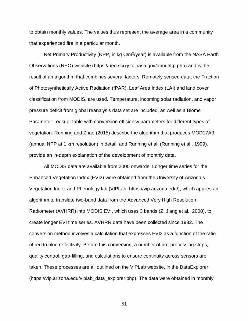
51
to obtain monthly values. The values thus represent the average area in a community
that experienced fire in a particular month.
Net Primary Productivity (NPP, in kg C/m2/year) is available from the NASA Earth
Observations (NEO) website (https://neo.sci.gsfc.nasa.gov/about/ftp.php) and is the
result of an algorithm that combines several factors. Remotely sensed data; the Fraction
of Photosynthetically Active Radiation (fPAR), Leaf Area Index (LAI) and land cover
classification from MODIS, are used. Temperature, incoming solar radiation, and vapor
pressure deficit from global reanalysis data set are included, as well as a Biome
Parameter Lookup Table with conversion efficiency parameters for different types of
vegetation. Running and Zhao (2015) describe the algorithm that produces MOD17A3
(annual NPP at 1 km resolution) in detail, and Running et al. (Running et al., 1999).
provide an in-depth explanation of the development of monthly data.
All MODIS data are available from 2000 onwards. Longer time series for the
Enhanced Vegetation Index (EVI2) were obtained from the University of Arizona’s
Vegetation Index and Phenology lab (VIPLab, https://vip.arizona.edu/), which applies an
algorithm to translate two-band data from the Advanced Very High Resolution
Radiometer (AVHRR) into MODIS EVI, which uses 3 bands (Z. Jiang et al., 2008), to
create longer EVI time series. AVHRR data have been collected since 1982. The
conversion method involves a calculation that expresses EVI2 as a function of the ratio
of red to blue reflectivity. Before this conversion, a number of pre-processing steps,
quality control, gap-filling, and calculations to ensure continuity across sensors are
taken. These processes are all outlined on the VIPLab website, in the DataExplorer
(https://vip.arizona.edu/viplab_data_explorer.php). The data were obtained in monthly

52
time steps and at a 0.05° resolution for 1982-2010. Area-weighted time series were
extracted for each community polygon. A number of corrections were applied to ensure
continuity between pre- and post-2000 data (see “Technical Validation”). Note that there
are differences between the earlier mentioned EVI records and these EVI2 records for
2000-2010 due to the different resolutions of the data, and the modifications applied at
the VIPLab.
At point level, monthly precipitation data (in mm) from stations were extracted
from the Global Historical Climatology Network (GHCN) by NOAA
(https://www.ncdc.noaa.gov/ghcnm/v2.php): 5 stations in Acre (Brazil), 1 in Madre de
Dios (Peru) and 2 in Pando (Bolivia). All these time series have gaps, ranging from a
few months to a full year.
Monthly minimum, maximum and average stream flow data (in m3/s) for the three
most important rivers in the area were also located and downloaded: for the Rio Acre
and Rio Madre de Dios. The data were obtained from the Agência Nacional de Águas
(ANA) in Brazil, through its Hidroweb (http://www.snirh.gov.br/hidroweb/ or
http://hidroweb.ana.gov.br/). Searches were conducted to find stations for two river
basins; Rio Acre is in the sub-basin numbered 13 by ANA (Solimôes), and Rio Madre
de Dios is in sub-basin 15 (Madeira). Both are part of the larger Amazon basin. The Rio
Acre forms the border between Peru and Brazil, and for a part between Bolivia and
Brazil (until Cobija/Brasiléia). Then it turns north, with the Rio Xapuri and Rio Branco
being tributaries before the river reaches the town of Rio Branco. From Cobija and
Brasiléia onwards part of the border is the the Rio Abuña, which is a tributary to the Rio
Madeira (in the state of Rondônia, Brazil). The Rio Madre de Dios originates in Peru,

53
flows into Bolivia and eventually joins the Rio Beni and the Rio Madeira. Most stations
have gaps in the data in varying degrees, and for 3 stations on the Rio Acre enough
data were available to apply a gap-filling method based on linear regression between
station data to create continuous time series.
At country level, annual indicators from the World Bank DataBank
(http://databank.worldbank.org/data/home.aspx) were compiled for the natural sub-
system: agricultural land, arable land and protected areas, all as percentage of the land
area in each country.
At the global level, monthly time series for the Atlantic Multidecadal Oscillation
(AMO), the Pacific Decadal Oscillation (PDO) and the Multivariate El Niño/Southern
Oscillation Index (MEI) were obtained from the NOAA Earth System Research
Laboratory (https://www.esrl.noaa.gov/psd/data/climateindices/list/). For the AMO we
obtained the unsmoothed version (Enfield et al., 2001). This time series is an index of
surface temperature of the North Atlantic Ocean. The PDO consists of the first principal
component of monthly anomalies of sea surface temperature of the North Pacific
Ocean(Mantua et al., 1997; Zhang et al., 1997). The MEI is a composite index that is
believed to better reflect the El Niño/Southern Oscillation (ENSO) phenomenon than
simply sea surface temperatures (Wolter and Timlin, 2012). It incorporates sea level
pressure, surface air temperature, sea surface temperature, cloudiness fraction, zonal
and meridional components of surface wind over the tropical Pacific Ocean.
Stationary Variables
Stationary data for the communities covered in this database are provided as
separate records. These records contain information on names, area, distances to
markets and capitals (see “Human variables”) and mean elevation (meters above sea

54
level, MASL). Mean elevation is extracted from a Digital Elevation Map (DEM) using the
“Zonal Statistics” tool in ArcGIS. This DEM was sourced from the website of the United
States Geological Society (USGS, http://gdex.cr.usgs.gov/gdex) associated with LP-
DAAC. Most importantly, this record with community information contains community
IDs that should be used to link the various files with country and community level data.
Forest types were available for the Acre area (Brazil) from a previous
study(Salimon et al., 2011) that used a combination of the Brazilian Forest Classification
System and the Vegetation map of the Ecological and Economical Zoning for Acre for
its classification. The latter vegetation map is based primarily on the Radambrasil
project (Projeto Radar da Amazônia), the first large-scale monitoring project in the
Amazon. This classification takes soil, climate geological and geomorphological
attributes into account. Using this classification, forest types were generated for Madre
de Dios (Peru) and Pando (Bolivia) with a Random Forest model that included the
covariates EVI, soils, elevation, and slope. Where forest is absent, the land cover is
classified as “developed” or as “water”. For each community, the percentage of forest
types and/or land cover is given.
Botanical data were collected for a number of sites in the area between 2007 and
2010 for studies on biomass(Baraloto et al., 2014) and forest value(Baraloto et al.,
2015). These articles provide an in-depth overview of methods used, a summary will be
provided here. Study sites were selected to represent geographic variability, and
community leaders were engaged to provide consent and identify areas representative
of the community area. Focus was on terra firme forests with the aim of being able to
evaluate human impacts. Across the whole MAP area 67 sites were sampled with an

55
adaptation of the Phillips et al. (Phillips et al., 2003) modified Gentry plot
method(Baraloto et al., 2011) in a paired design, with the purpose of measuring
biodiversity and aboveground biomass. There were 27 sites in Acre, 25 in Madre de
Dios and 15 in Pando. Distance from roads varied, with generally one site closer to
roads (< 2 km) and 1 further away (> 5 km) in each community. Each site consisted of a
100 x 190 m sampling grid, within which 10 subplots of 2 x 50 m were sampled. The
subplots were situated perpendicular to a randomly chosen baseline, alternatively
opposite of each other along this baseline. Woody plants with a diameter at breast
height (DBH, at 1.3 m) ≥ 2.5 cm were measured for height and DBH. Then, each
subplot was extended to 10 x 50 m, and all woody stems with DBH ≥ 20 cm were
measured. Voucher specimens were collected for species that could not be identified in
the field, and collections from each country are held at their local herbaria: the National
Amazonian University of Madre de Dios in Puerto Maldonado (Peru), the Center for
Research on Amazon Protection of the Amazonian University of Pando in Cobija
(Bolivia), and the Zoobotanical Park of the Federal University of Acre in Rio Branco
(Brazil). After extensive identification efforts, 93.5% of samples were identified to the
genus level, 99.5% to the family level. In addition to detailed plant data, aboveground
biomass and biomass in timber species were calculated per site. Aboveground biomass
was estimated with allometric equations based on size class as per Baraloto et al.
(Baraloto et al., 2011).
To obtain soil information for the area, a gridded soil data set was downloaded
from the International Soil Reference and Information Centre (ISRIC – World Soil
Information, http://www.isric.org/explore/soilgrids). This data set has a resolution of 1

56
km and provides soil organic carbon (g/kg), soil pH, sand, silt and clay fractions (%),
bulk density (tones/m3), cation-exchange capacity (cmol/kg), volumetric coarse
fragments, soil organic carbon stock (tonnes/ha), depth to bedrock (m), World
Reference Base soil groups and USDA Soil Taxonomy suborders at 6 depths covering
0-200 cm soil profiles(Hengl et al., 2014). For this database, we averaged the 6 values
to obtain single values. Values for saturated hydraulic conductivity (10-6 m/s), saturated
volumetric water content and residual volumetric water content (both cm3/cm3) were
calculated with pedotransfer functions listed in Marthews et al. (Marthews et al., 2014),
using those by Cosby et al. (1984 in Marthews et al., 2014) for saturated hydraulic
conductivity and those by Tomasella and Hodnett (1998 in Marthews et al., 2014) for
water content. Information for each community was extracted using GIS.
Shapefiles are made available as well, these include: state boundaries,
communities, roads, rivers and protected areas. The metadata for the point data (flow
and precipitation from stations) provide coordinates for the stations.
Data Records
All data sets and records are stored in a Figshare repository, (Data Citation 1:
10.6084/m9.figshare.c.3933364). The main level of data organization is under the
headers human variables, natural variables and stationary data (Table 2-1). Within
these, there are subdivisions. Under “human variables”, data are grouped at either
community or country level. Table 2-1 lists the available data and their level, and files
are named according to the listed abbreviation. All data are provided in comma
delimited files (.csv), with either a country or community identifier. Where necessary,
metadata files are included to elaborate on data in the files. Environmental variables
have a similar format and organization, and also contain data at global or point level.

57
Data at global level (climate indices) are not linked to any country or community. Point
data files contain coordinates for their location in a metadata file, including station
numbers. Separate files contain the data per station. For precipitation this is all
contained in one file, but since flow data contain a number of time series (minimum,
maximum and mean), it is separated per station. These files are also comma delimited
files (.csv). Dynamic variables that have a temporal resolution of 1 month contain a
column for months and a column for years to reduce issues with reading dates into data
analysis programs. The time periods for which data are available varies, see Table 2-1.
Stationary data are a mix of comma delimited files (.csv) and shapefiles (.shp
and associated files). Data are grouped for community information, botanical data,
forest type, shapefiles and soil type (Table 2-2). All metadata files are comma delimited
as well.
Technical Validation
Data from reanalysis projects or larger global data sets were sourced from
reputable sources (e.g. WorldBank data, data from NOAA, CRU, ISRIC) with internal
data checks. Other local data were obtained from sources with documentation on
measurements and calculations (e.g. ANA, GHCN). We double-checked coordinates for
the stations to ensure that they were in the MAP area and along water ways (for the
flow data). In addition, visual checks of data relating to dynamic variables was done to
ensure there were no anomalous data. Where there were minor issues with community
data relating to human variables (e.g. travel times, family density), these were identified
and resolved in an iterative manner due to several authors evaluating the data sets.
Note that some station data (precipitation and stream flow) have gaps.

58
Data correction was performed on EVI2 data to address outliers and
discrepancies between AVHRR-derived EVI (1982-1999) and MODIS EVI (2000-2010),
because AVHRR-derived EVI exhibited consistently lower values. This is attributed to
the lower quality of AVHRR data in areas with high cloud density (pers. comm. Dr. K.
Didan). For this correction, data were divided into pre- and post-2000 data. For each
data group, outliers were defined as an uncharacteristically positive change from one
month to the other, shaped as a peak. Negative changes were not scrutinized, since
vegetation can be cut down, causing a large negative change in EVI. However, it would
be unlikely for EVI to peak very quickly. Any change larger than 2 times the interquartile
range of the data is flagged and removed. The change value was purposefully kept
large since the data had already undergone pre-processing at the VIPLab. Removed
values were replaced with long-term averages on a month-by-month basis (i.e. a gap for
January was filled with the long-term average for January). Finally the pre-2000 data set
was adjusted by moving the data up by the long-term post-2000 average, again on a
month-by-month basis for each community separately. This was done on a month-by-
month basis because differences between the long-term averages varied per month
(Figure 2-1). The data repository contains an RMarkdown file with code and this
explanation.
We highly encourage users to consult the original sources, websites and
publications for general data limitations and caveats. While all reanalysis and calculated
data comes from reputable sources, underpinned by peer-reviewed publications, users
should familiarize themselves with these and take these into account during and after
analyses. All variables have been captured and recorded in the International System of

59
Units (SI). Note that Portuguese or Spanish names can include special characters that
do not transfer well into coding or analysis applications.
Usage Notes
As the impact of human disturbances increases and intensifies in many areas
due to road infrastructure development, it is important to be able to analyze systems as
a broad as possible. Considering systems as coupled natural-human systems that are
dynamic over time and space allows researchers to fully explore what kinds of impacts
to expect. We would like to encourage researchers to use these data in explicit spatio-
temporal approaches, integrating human and natural variables. While a number of
studies have already been conducted with these data, each mostly considered separate
components of the data set. Of particular interest for future research would be changes
over time in the system associated with road infrastructure development. These data
could also be used to investigate spatial variability and heterogeneity in relation to road
infrastructure. With the available data, analyses can take place at the regional level, or
at community level. Of interest could be:
1. Time series research on dynamic variables to understand the interplay between variables and find drivers or causality mechanisms;
2. Simulation and prediction studies to identify important variables, and the potential for system state changes. This type of research would be informative for other areas undergoing road infrastructure development in terms of types of models to use and data collection requirements;
3. Global Sensitivity and Uncertainty Analyses to understand the workings of these models. The data in this database can provide a baseline for the development of distributions required for model parameters.
.

60
Table 2-1. Overview of dynamic variables collected and compiled for the area in Madre de Dios (Peru), Acre (Brazil) and Pando (Bolivia), the MAP area.
Sub-system
Spatial resolution
Dynamic Variables Temporal resolution
Time period H
UM
AN
Community ENF Enforcement of tenure rules (0 to 1: with 0=least, 1=most)
Annual 1985 - 2010
Country ENR Electricity from non-renewable sources (oil, gas and coal; % of total)
Annual 1980 – 2010
Country ER Electricity from renewable sources, excluding hydroelectric (% of total)
Annual 1980 - 2010
Community FAM Number of families in the community
5-yearly 1987 - 2012
Community FAMD Family density (families/km2) 5-yearly 1987 - 2012
Country FI Foreign direct investment, net inflows (% of GDP)
Annual 1980 - 2011
Country FR Profit from forests (% of GDP) a Annual 1980 - 2010
Country GDP GDP growth (annual %) Annual 1980 – 2011
Country GDPC GDP per capita growth (annual %) b
Annual 1980 - 2011
Country GR Profit from natural gas (% of GDP) c
Annual 1980 - 2010
Country LE Life expectancy at birth, total (years)
Annual 1980 – 2011
Country MR Profit from minerals (% of GDP) d
Annual 1980 – 2010
Country NRR Total profit from natural resources (% of GDP) e
Annual 1980 - 2010
Country OR Profit from crude oil (% of GDP) f
Annual 1980 – 2010
Country PC Power consumption (kWh per capita)
Annual 1980 - 2010
Community PNC Population in (nearest) state capital
Annual 1986 – 2010
Community PNM Population in nearest market Annual 1986 - 2010
Country PPP
GDP per capita, PPP (current international $) = GDP converted to international dollars using purchasing power parity rates
Annual 1980 - 2011
Community PAV Paving (0 to 1, with 0=no paving, 1=fully paved)
Annual 1985 - 2012
Community TEN
Percentage of deforestation allowed under tenure rules (0 to 1: e.g. 0.1=maximum of 10% deforestation allowed)
Annual 1985 - 2010
Community TTC Travel time to capital (minutes) Annual 1986 - 2010
Community TTM Travel time to nearest market (minutes)
Annual 1986 - 2010

61
Table 2-1. Continued. Sub-system
Spatial resolution
Dynamic Variables Temporal resolution
Time period N
AT
UR
AL
Country AG Agricultural land (% of land area) g
Annual 1980 - 2009
Global AMO Atlantic Multidecadal Oscillation Monthly 1987 - 2009
Country AR Arable land (% of land area) h Annual
Community EVI Enhanced Vegetation Index (MODIS product)
Monthly 2000 - 2010
Community EVI2 Enhanced Vegetation Index 2 (VIPLab product)
Monthly 1982 - 2010
Community FIR Fire occurrence (average over a community area per month)
Monthly 2000 - 2010
Point FLOW River flow at a number of stations
Monthly* ~1967 - 2012*
Community FOR Forest area as percentage of community area
5-yearly 1986 – 2010
Community MAXT Maximum temperature (°C) Monthly 1982 - 2010
Community MEANT Mean temperature (°C) Monthly 1982 - 2010
Global MEI Multivariate ENSO Index Monthly 1987 - 2009
Community MINT Minimum temperature (°C) Monthly 1982 - 2010
Community NPP Net Primary Production (C/m2/year)
Monthly 2000 - 2010
Community P Precipitation (mm) Monthly 1982 - 2010
Country PA Percentage Protected Areas (% of whole country)
Annual 1980 - 2009
Global PDO Pacific Decadal Oscillation Monthly 1987 - 2009
Point PP Precipitation (mm) at a number of meteorological stations
Monthly* ~1985 - 2011*
Community PET Potential evapotranspiration (mm)
Monthly 1982 - 2010
Community SM Soil moisture (mm) Monthly 1982 - 2010
Community SR Species richness (alpha diversity) i
Annual 1984 - 2012
a Also called ‘forest rents’, defined as the roundwood harvest multiplied with the product of average prices and a region-specific rental rate. b GDP per capita based on purchasing power parity (PPP). PPP GDP is gross domestic product converted to international dollars using purchasing power parity rates. An international dollar has the same purchasing power over GDP as the U.S. dollar has in the United States. GDP at purchaser's prices is the sum of gross value added by all resident producers in the economy plus any product taxes and minus any subsidies not included in the value of the products. It is calculated without making deductions for depreciation of fabricated assets or for depletion and degradation of natural resources. Data are in current international dollars. c Also called ‘natural gas rents’: the difference between the value of natural gas production at world prices and total costs of production. d Also called ‘mineral rents’: the difference between the value of production for a stock of minerals at world prices and their total costs of production. Tin, gold, lead, zinc, iron, copper, nickel, silver, bauxite and phosphate are included. e Also referred to as ‘total natural resources rents’: the sum of oil rents, natural gas rents, coal rents, mineral rents and forest rents. f ‘Oil rents’: the difference between the value of crude oil production at world prices and total cost of production.

62
Table 2-1. Continued. g Agricultural land refers to the share of land area that is arable, under permanent crops, and under permanent pastures. Land under permanent crops is land cultivated with crops that occupy the land for long periods and need not be replanted after each harvest, such as cocoa, coffee, and rubber. This category includes land under flowering shrubs, fruit trees, nut trees, and vines, but excludes land under trees grown for wood or timber. Permanent pasture is land used for five or more years for forage, including natural and cultivated crops. h Arable land includes land defined by the FAO as land under temporary crops (double-cropped areas are counted once), temporary meadows for mowing or for pasture, land under market or kitchen gardens, and land temporarily fallow. Land abandoned as a result of shifting cultivation is excluded. i Alpha diversity translated into number of species per polygon, inferred from Landsat data by Convertino et al. (2012). * Some time series have gaps, for flow 3 stations have been gap-filled (see ‘Methods’). Time series vary in length for each station
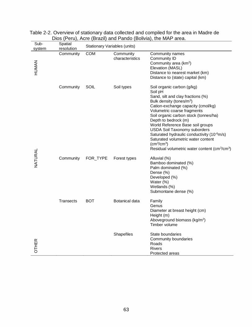
63
Table 2-2. Overview of stationary data collected and compiled for the area in Madre de Dios (Peru), Acre (Brazil) and Pando (Bolivia), the MAP area.
Sub-system
Spatial resolution
Stationary Variables (units)
HU
MA
N
Community COM Community characteristics
Community names Community ID Community area (km2) Elevation (MASL) Distance to nearest market (km) Distance to (state) capital (km)
NA
TU
RA
L
Community
SOIL Soil types Soil organic carbon (g/kg) Soil pH Sand, silt and clay fractions (%) Bulk density (tones/m3) Cation-exchange capacity (cmol/kg) Volumetric coarse fragments Soil organic carbon stock (tonnes/ha) Depth to bedrock (m) World Reference Base soil groups USDA Soil Taxonomy suborders Saturated hydraulic conductivity (10-6m/s) Saturated volumetric water content (cm3/cm3) Residual volumetric water content (cm3/cm3)
Community
FOR_TYPE Forest types Alluvial (%) Bamboo dominated (%) Palm dominated (%) Dense (%) Developed (%) Water (%) Wetlands (%) Submontane dense (%)
Transects BOT Botanical data Family Genus Diameter at breast height (cm) Height (m) Aboveground biomass (kg/m2) Timber volume
OT
HE
R
Shapefiles State boundaries Community boundaries Roads Rivers Protected areas

64
Figure 2-1. Comparison of monthly values per community polygon for AVHRR-derived EVI (1982-1999) and “true” EVI (2000-2010). A) Monthly averages for 2 periods. B) Differences between the monthly averages for the 2 periods.

65
CHAPTER 3 CLUSTER ANALYSIS OF VEGETATION DYNAMICS AND ASSOCIATION WITH
ROAD PAVING
Background
The Amazon region in South America holds the largest areas of intact forest in
the world and has been proven to be of great importance to the global climate system
and biodiversity (Foley et al., 2007; Keller, 2009). There is global concern about
changes in land cover in the Amazon caused by anthropological disturbances and the
consequences of such land cover changes; both globally and locally (Davidson et al.,
2012; Keller, 2009; Nobre and Borma, 2009). Anthropological disturbances have an
impact directly on forest cover by deforestation, but also on forest structure and
composition, varying with the extent and frequency of the disturbances. Structural and
phenological changes due to anthropological disturbances (logging, fire) are for
instance changes in basal area, community composition (J. Zhu et al., 2007),
understory composition and vine cover (Felton et al., 2006). Infrastructure development,
such as road building, increases these disturbances and many studies have highlighted
negative socio-economic and biophysical effects that these developments have at local,
regional and even larger scales. Road paving and construction has been found to be
the main driver of deforestation (Laurance et al., 2009; 2002c). Other effects include
land degradation, impacts on abiotic processes (such as hydrology), disruption of
movement of organisms and increased mortality, alteration of natural disturbance
regimes (e.g. fire), pollution, violent conflict over natural resources, and rural-urban
migration (Coffin, 2007; Laurance et al., 2009; Marsik et al., 2011; Perz et al., 2011b;
2011a).

66
The Inter-Oceanic Highway (IOH) runs through the forested and highly biodiverse
‘MAP’ area in the SW Amazon, a tri-national area that includes parts of Peru, Brazil and
Bolivia, for which we gathered a large multi-disciplinary long-term database. Paving of
the highway has started at different times across the area, offering a valuable study site
with data before, during and after anthropological disturbance. Considering the tight
coupling of natural and human systems in this area, changes in ecosystem services
from the natural (forest) system would have far-reaching consequences. This concern
goes beyond deforestation or forest loss: even if forest cover is maintained, is this forest
degraded or altered over time due to road paving? Degradation of the forest ecosystem
has an effect on ecosystem services, and in order to evaluate degradation, we propose
to look at vegetation dynamics in this study. Vegetation dynamics, or phenology, refer to
the timing of biological processes, such as flowering, growth and senescence.
Vegetation structure and species composition have an effect on vegetation dynamics,
and vegetation dynamics in turn affect ecosystem services such as primary productivity
and nutrient cycling (Figure 1-1). If a change in vegetation dynamics is found, we can
deduct that ecosystem services broadly will also have changed.
We use the extended Enhanced Vegetation Index (EVI2), a remote sensing
product, as a proxy for vegetation dynamics. This product is an extended version of
original EVI (which is available from 2000 onwards), with values as far back as 1982
obtained from a conversion of other remote sensing data (form the Advances Very High
Resolution Radiometer). Previous research on vegetation dynamics in the Amazon
created ‘pheno-regions’ using the Normalized Difference Vegetation Index (NDVI),
within which phenology is similar (F. B. Silva et al., 2013). Similarly, this study aims at

67
‘grouping’ vegetation dynamics time series and assesses these dynamics at a smaller
scale, particularly in the presence of road paving. Road paving introduces new and
amplified perturbations to the system (Cumming et al., 2005), thus we hypothesize that
vegetation dynamics are affected by road paving over time. We expect that similar
vegetation dynamics (in terms of values and timing) can be grouped together, and that
they are associated with the extent of road paving. Since the data cover areas with
roads that were paved at the beginning of the study period (1987 – 2009), areas that
had roads paved over the course of the study period and areas that never had paved
roads, we expect to identify different (transitional) states of vegetation dynamics.
To answer this hypothesis, we use time series of EVI2 to explore potential
clusters, and the characteristics of these clusters. Considering the size of our overall
data set and further research, the additional advantage is the reduction of complexity of
the data set. Cluster analysis is a useful method to deal with large data sets, to gain
initial understanding of the structure and potential relationships, before proceeding to
more complex analyses. Specific methods have been developed to cluster time series.
Some of the best known are Dynamic Time Warping (DTW) and shape-based distance
(SBD). For the purpose of our research, a method was needed that clusters time series
together based on timing of values specifically, not just frequencies. We wanted to
ensure that vegetation dynamics that peak or fall in a particular month were clustered
together: the focus is on similarity in phenological variation. Hence, for the creation of a
dissimilarity matrix – on which clustering is based – this needs to be accounted for. In
this study, we used a method that creates an adaptive dissimilarity index: this takes into
account both values and ‘behavior’ of the time series (Chouakria and Nagabhushan,

68
2007). After clustering the data with a number of hierarchical methods, we employed
two validation measures that supply criteria for the optimum number of clusters and
clustering method based on compactness and separation (Figure 3-2). In order to
investigate if there were biophysical variables that had the potential explain the cluster
results for EVI2, we applied cluster analysis to the data sets for minimum, maximum
and mean temperature, precipitation, soil moisture, potential evapotranspiration and
species richness. We also took into account values and behavior (similar to the EVI2
clustering), and evaluated if the results were similar to EVI2 clustering
To investigate cluster differences, mean and median values for the EVI2 per
cluster are not useful, since a) all analyses were and will be done on normalized data, to
focus on the dynamics, and b) the dissimilarity index takes dynamics into account as
well as actual values. Neither does comparing variance provide much information, since
these values can be the same, but the timing can differ. We decided to look at the
number of ‘states’ for each cluster in terms of EVI2 values. States are defined as the
dominant values, i.e. peaks in the probability distribution of the values. By defining these
using a moving window over the whole study period, we can see if the number of states
change over time. We applied a breakpoint analysis to assess differences between the
clusters.
Methods
Data
For this analysis we primarily focused on time series for EVI2, the long-term EVI
data set with AVHRR-converted EVI data for the period pre-2000. We used monthly
time series for road paving, minimum, maximum and mean temperature, precipitation,
PET, soil moisture and species richness to attempt to interpret the cluster results. These

69
data sets are described in detail in Chapter 2. For these analyses, we used monthly
data from January 1987 to December 2009, considering that this was the time frame for
which data described in Chapter 2, and to be used in subsequent Chapters, overlaps.
Figure 3-1 shows average values over this time period for each community in the study
area. It gives an indication of the differences in average values, but in this study we did
not use absolute values. All data were normalized, since we are only interested in
dynamics – shape and relative magnitude of values – not absolute values.
Time Series Clustering Based on an Adaptive Dissimilarity Index
All clustering methods start with developing a matrix that contains distances
between points or objects (Figure 3-2). For clarification, in this text we refer to this
matrix as the dissimilarity matrix (other terms are distance, similarity or proximity
matrix). Each time series in the analysis is called an object. The dissimilarity measure
we calculate is related to closeness of values and time series behavior (Chouakria and
Nagabhushan, 2007), which is achieved by including an automatic adaptive tuning
function in the conventional dissimilarity index:
𝐷(𝑆1, 𝑆2) = 𝑓(𝑐𝑜𝑟𝑡(𝑆1, 𝑆2)) ∙ 𝛿𝑐𝑜𝑛𝑣(𝑆1, 𝑆2) (3-1)
with
𝑓(𝑥) =2
1+𝑒𝑘∙𝑥 , 𝑥 ≥ 0 (3-2)
in which S is an object (a time series) and 𝑘 a parameter that determines how much 𝑥 is
taken into account, with 𝑥 being the temporal correlation coefficient (𝑐𝑜𝑟𝑡(𝑆1, 𝑆2), see
Equation 3-4). At a value of 𝑘 = 0, the dissimilarity matrix is based on values only. At
higher 𝑘, temporal correlation (‘behavior’) is taken into account more. The conventional
measure for dissimilarity based on values is expressed in 𝛿𝑐𝑜𝑛𝑣(𝑆1, 𝑆2) which is the

70
summed Euclidian distance between series 𝑆1 and 𝑆2 at 𝑡𝑖 with respective values 𝑢 and
𝑣 for 𝑝 points in time:
𝛿𝑐𝑜𝑛𝑣(𝑆1, 𝑆2) = √(∑ (𝑢𝑖 − 𝑣𝑖)2𝑝𝑖=1 ) (3-3)
The temporal correlation coefficient that is used in Equation 3-1 is:
𝑐𝑜𝑟𝑡(𝑆1, 𝑆2) =∑ (𝑢𝑖+1−𝑢𝑖)(𝑣𝑖+1− 𝑣𝑖)
𝑝−1𝑖=1
√∑ (𝑢𝑖+1−𝑢𝑖)2𝑝−1𝑖=1
√∑ (𝑣𝑖+1−𝑣𝑖)2𝑝−1𝑖=1
(3-4)
where 𝑐𝑜𝑟𝑡(𝑆1, 𝑆2) lies between -1 and 1. At 1, series 𝑆1 and 𝑆2 exhibit exactly the same
behavior between 𝑡𝑖 and 𝑡𝑖+1: increase or decrease with the same growth rate. At 0 their
growth rates are stochastically linearly and independent, and at -1 their behavior is
opposite. Parameter k determines how much proximity with respect to behavior or with
respect to value contributes to the dissimilarity index.
After developing dissimilarity matrices for a range of values for 𝑘 (0 ≤ 𝑘 ≤ 5),
hierarchical agglomerative clustering was applied. This method takes a bottom-up
approach, starting with each object as a singleton cluster. At each step, clusters merge
based on certain distance metrics, until all objects are clustered in one cluster. The
resulting cluster tree or dendrogram can then be evaluated to decide where to cut off
the tree. We evaluated the results of four cluster methods: single linkage, complete
linkage (maximum), average linkage and Ward’s method. In single linkage clustering,
the clusters with the smallest minimum pair-wise distance (between objects in different
clusters) are clustered together at each step. Complete linkage clustering is also based
on pairwise distances, but it clusters those together that have the smallest maximum
distance. This method is more sensitive to outliers. Average linkage clustering
calculates the average distance between all objects in one cluster and all objects in

71
another cluster, and clusters based on the smallest value. Ward’s method takes a
different approach than these three methods: instead of using distance metrics, it
analyzes variance. For each possible combination of clusters at a step, the error sum of
squares (ESS) is calculated, and whichever pair yields the smallest ESS is clustered
together. The ESS thus compares individual objects against cluster means. With objects
𝑘 with dissimilarity values 𝑥 in cluster 𝑖 it is calculated as:
𝐸𝑆𝑆 = ∑ ∑ |𝑥𝑖𝑘 − �̅�𝑖𝑘|2𝑘𝑖 (3-5)
This implies that the initial cluster distance (between singleton clusters) is the Euclidean
squared distance between objects. For each cluster method, we evaluated the results of
2 to 10 clusters, for dissimilarity matrices with 𝑘 ranging from 0 to 5 for each (a total of
216 cluster options), Figure 3-2.
Clustering Validation Measures
The Dunn Index (Dunn, 2008) and the Silhouette Width (Rousseeuw, 1987) were
used as metrics to determine the suitability of the clusters. These are widely used
metrics that focus on compactness and separation of clusters. They are known as
internal validation measures: evaluation of the clusters is based on the data and
clustering only and no additional (‘outside’) information is required.
The number of clusters with the highest Dunn index (DI) indicates this the
optimum number of clusters; i.e. the highest separation between clusters, and the least
spread of data within clusters. The index is the ratio of the minimum distance between
observations not in the same cluster, and the maximum distance between observations
within a cluster. This can be written as
𝐷𝐼 =min𝑖≠𝑗
{𝛿(𝐶𝑖,𝐶𝑗)}
max1≤𝑙≤𝑘
{∆(𝐶𝑙)} (3-6)

72
where 𝛿(𝐶𝑖 , 𝐶𝑗) is the distance between clusters 𝑖 and 𝑗, and ∆(𝐶𝑙) is the within-cluster
distance (the diameter) for a cluster with 𝑘 objects.
The Silhouette width (SW) ranges from -1 to 1, with higher values meaning that
the clusters are cohesive and well separated. This measure takes the lowest average
dissimilarity of a series with other clusters (Euclidean distance) and subtracts the
average dissimilarity of the series with its own cluster. The “silhouette” is then the ratio
of this number to whichever average dissimilarity is the highest: if the average
dissimilarity with the neighboring cluster is larger than the average dissimilarity within-
cluster, this yields a positive number ≤ 1. The average silhouette is the final metric. For
instance, for a system with cluster 𝐴 and a number of clusters 𝐶 (for which 𝐶 ≠ 𝐴), the
calculation of silhouette 𝑠 for object 𝑖 in 𝐴 is (Rousseeuw, 1987):
𝑎(𝑖) = 𝑎𝑣𝑒𝑟𝑎𝑔𝑒 𝑑𝑖𝑠𝑠𝑖𝑚𝑖𝑙𝑎𝑟𝑖𝑡𝑦 𝑜𝑓 𝑖 𝑡𝑜 𝑎𝑙𝑙 𝑜𝑡ℎ𝑒𝑟 𝑜𝑏𝑗𝑒𝑐𝑡𝑠 𝑜𝑓 𝐴 (3-7)
𝑑(𝑖, 𝐶) = 𝑎𝑣𝑒𝑟𝑎𝑔𝑒 𝑑𝑖𝑠𝑠𝑖𝑚𝑖𝑙𝑎𝑟𝑖𝑡𝑦 𝑜𝑓 𝑖 𝑡𝑜 𝑎𝑙𝑙 𝑜𝑏𝑗𝑒𝑐𝑡𝑠 𝑜𝑓 𝑒𝑎𝑐ℎ 𝐶 (3-8)
After calculating this for all clusters 𝐶 ≠ 𝐴, we find the smallest value:
𝑏(𝑖) = min𝐴≠𝐶
𝑑(𝑖, 𝐶) (3-9)
and calculate silhouette 𝑠(𝑖):
𝑠(𝑖) =𝑏(𝑖)−𝑎(𝑖)
max{𝑎(𝑖),𝑏(𝑖)} (3-10)
this can then be average for all objects 𝑘 in 𝐴
𝑠𝑘 =1
𝑛𝑘∑ 𝑠(𝑖) (3-11)
and eventually be averaged for all clusters.
The package ‘clValid’ in R was used for analyses, with changes made to the
code so they could use the previously described adaptive dissimilarity matrix.

73
Number of States and Breakpoint Analysis
After cluster analysis, EVI2 time series were grouped together in their respective
cluster. They were then averaged in an area-weighted manner for each cluster for this
analysis, based on the area of the community the EVI2 time series is associated with.
We developed histograms and calculated the probability distribution functions over a
moving window of 5 years (60 months) for each area-weighted time series. The number
of peaks in the histogram were counted and noted as ‘states’ for that particular window.
Moving the window one month at a time, all states were recorded for the full period of
record. This method has been applied in the past theoretical systems such as Lorenz
curves (Huffaker et al., 2017) - from which the code has been derived - and a similar
approach has been used on climate systems (Livina et al., 2010). Since the number of
states appeared to vary over time, we applied a break point analysis (Andersen et al.,
2009; Zeileis et al., 2003; 2002) to determine the point where there was a statistically
significant difference in number of states between two periods. This is termed a
‘structural change’.
The ‘strucchange package’ in R (Zeileis et al., 2002) was used to perform the
breakpoint analysis. The method we implemented relies on F test statistics, and tests
for a single breakpoint – across the whole time period of interest, for each potential
change point. This test is also known as a Chow test: for a particular point in time two
linear models are fitted – one for the data before this point and one for data after that
point. The resulting residuals are then compared to the residuals from a linear model
fitted for the complete time series. If n is the number of observations and k the number
of regressors in the model,

74
𝐹 =𝑅𝑆𝑆−𝐸𝑆𝑆
𝐸𝑆𝑆 (𝑛−2𝑘)⁄ (3-12)
with RSS the restricted sum of squares (residuals from one model for all observations)
and ESS the error sum of squares (residuals from a model with two components). In our
analyses, the linear model was a model without a slope, hence the mean of the time
series. The implemented approach uses moving breakpoints, thus generating
sequential F tests. The year for which the F statistic is highest (and above the critical F
level), is regarded as the breakpoint (Andersen et al., 2009; Zeileis et al., 2003). To
determine whether a breakpoint is statistically significant (above the critical F level), p-
values are calculated – which are adjusted for asymptotic p-value approximations
(Hansen, 1997).
Data Availability
The data sets generated during and/or analysed for this study, as well as code,
are available in a Figshare repository, 10.6084/m9.figshare.c.3933367.
Results
Four EVI2 Clusters Along a Road Paving Gradient
The validation measures that were calculated for all possible clusters, indicated
that all options were valid clusters, i.e. their values were larger than zero. DI and SW
are low overall, indicating that the clustering is weak to moderate. In determining the
appropriate number of clusters, we first looked for results where the optimum number of
clusters recommended by the DI and SW were the same (Table 3-1 and Figure 3-3).
While a number of clustering methods indicated that two clusters gave the highest DI
and SW, we decided to cluster the data into four clusters – the result from clustering
with Ward’s method (Figures 3-3 and 3-4). Since we are interested in finding and
75
analyzing heterogeneity in the study area, having more clusters essentially allows us to
analyze the data at a higher resolution. We opted to use the results from the analysis
that used 𝑘 = 2 in the adaptive dissimilarity index calculations. While the SW is lower
than for the option with 𝑘 = 3, the DI is almost twice as large. Since the DI seems to
take into account outliers more (since it takes the maximum within-cluster distance), we
preferred this value to be higher. At 𝑘 = 2 the contribution of the behavior component to
the dissimilarity index is 76.2% and the value component contributes 23.8% (Chouakria
and Nagabhushan, 2007).
After deciding on the appropriate number of clusters, the results were mapped
(Figures 3-5a and 3-5b). The resulting clusters showed spatial cohesion and will be
referred to as Vegetation Dynamics Clusters (VDCs). We calculated the mean road
paving extent per community (one value per community, Figures 3-5c and 3-5e), and
area-weighted average paving extent per VDC (a time series per cluster, Figure 3-5d).
We then ordered the VDCs accordingly: there was an increasing tendency in median
paving extent across VDCs (Figure 3-5e). There were also distinct differences in area-
weighted average paving extent per VDC (Figure 3-5d) in terms of start and end time of
paving. Road paving extent is indicated by values between 0 and 1, with 0 indicating an
unpaved road, 1 a fully paved road, and anything in between indicating road paving in
progress. Based on these distinctions, VDC 1 represents the unpaved system state,
VDC 2 and VDC 3 transition states, and VDC 4 the mostly paved system state.
Additional Cluster Analysis on Biophysical Variables
To test whether there were biophysical variables that could be associated with
the clustering found for EVI2, these were also clustered with the same methods and

76
evaluation metrics. We applied the same cluster analysis (with 𝑘 = 2 for the adaptive
dissimilarity index calculation) to the time series for minimum, maximum and mean
temperature, precipitation, PET, soil moisture and species richness. The optimum
number of clusters suggested by the DI and SW were not identical to EVI2 (Table 3-2).
States and Breakpoint Analysis
The number of states was variable for each VDC over time (Figure 3-6). For
VDCs 1, 2 and 3 the number of states is generally lower (2 to 3) at the end of the study
period. The breakpoint analysis found statistically significant breakpoints for each VDC,
which were all located between 1997 and 2001. We added the point in time where
average area-weighted paving was at 0.1 (10%) to Figure 3-6 to compare it with the
timing of the breakpoint.
Discussion
Assessment of Final Clusters
The DI and SW values indicate that overall, clustering is weak to moderate. This
is a result of the noisiness of the EVI2 data, something that is a problem with much
remote sensing data in the tropics (Huete et al., 2002). However, all cluster results are
valid in the sense that the DI and SW are positive values. Negative values would
indicate that clusters are overlapping, and that assignment of an object to a cluster is
probably misspecified. The moderate clustering strength is something to take into
account with further analyses. There might be outliers for each cluster that could
complicate analyses or interpretation of results. Spatially, one such outlier is potentially
the community in Bolivia (without paving) that has been clustered together with the
communities in Brazil (VDC 4). Still, from field work it appears that this community is
closely associated with the Brazilian communities, so even though it has no road paving
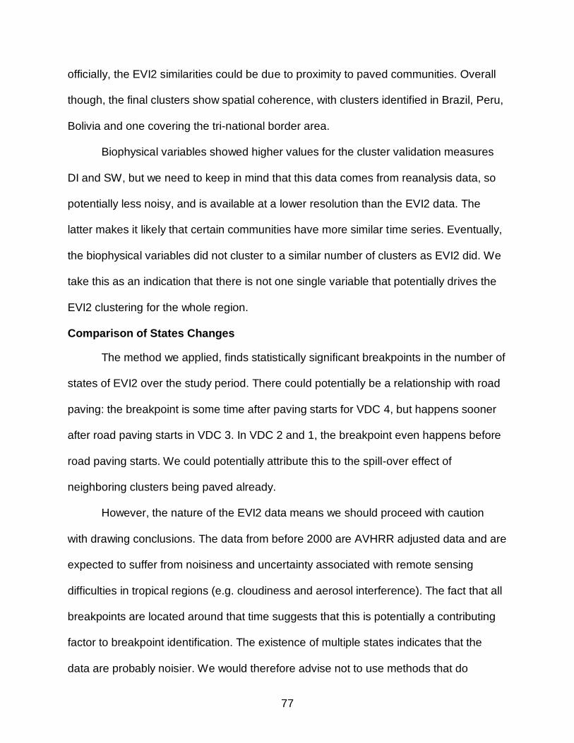
77
officially, the EVI2 similarities could be due to proximity to paved communities. Overall
though, the final clusters show spatial coherence, with clusters identified in Brazil, Peru,
Bolivia and one covering the tri-national border area.
Biophysical variables showed higher values for the cluster validation measures
DI and SW, but we need to keep in mind that this data comes from reanalysis data, so
potentially less noisy, and is available at a lower resolution than the EVI2 data. The
latter makes it likely that certain communities have more similar time series. Eventually,
the biophysical variables did not cluster to a similar number of clusters as EVI2 did. We
take this as an indication that there is not one single variable that potentially drives the
EVI2 clustering for the whole region.
Comparison of States Changes
The method we applied, finds statistically significant breakpoints in the number of
states of EVI2 over the study period. There could potentially be a relationship with road
paving: the breakpoint is some time after paving starts for VDC 4, but happens sooner
after road paving starts in VDC 3. In VDC 2 and 1, the breakpoint even happens before
road paving starts. We could potentially attribute this to the spill-over effect of
neighboring clusters being paved already.
However, the nature of the EVI2 data means we should proceed with caution
with drawing conclusions. The data from before 2000 are AVHRR adjusted data and are
expected to suffer from noisiness and uncertainty associated with remote sensing
difficulties in tropical regions (e.g. cloudiness and aerosol interference). The fact that all
breakpoints are located around that time suggests that this is potentially a contributing
factor to breakpoint identification. The existence of multiple states indicates that the
data are probably noisier. We would therefore advise not to use methods that do

78
comparisons on EVI2 data of pre- and post-paving periods. Since VDCs also cluster
along an average road paving gradient (Figure 3-5), an appropriate approach would be
to interpret the VDCs as areas increasingly impacted by road paving.
This research confirmed the hypothesis, that there are states associated with
road paving – but we do not have complete certainty about transitions. The state
changes and breakpoint analysis suggest an ordering along the road paving gradient,
but the noisiness of the EVI2 data requires that we interpret these results carefully.
Methodological Findings: Cluster Selection and State Changes
Selection of clustering is seldom straightforward, and we used two well-known
methods to evaluate clusters based on compactness and distance from other clusters.
While these methods should help in making the decision on the number of clusters less
subjective, choosing evaluation or validation measures is in itself also subjective – since
many exist. Using two methods, however, is a good safeguard against subjectivity. We
expected that the two measures would be more in agreement though, since they purport
to evaluate similar things; compactness and separation. The type of calculations applied
for each measure appear to result in differences though. Hence, in choosing the
appropriate number of clusters, it is also important to evaluate the validation measure
that is used by applying more than one measure and comparing results.
The method of finding state changes is a useful tool to better understand
dynamic data. In this study, however, the nature of the EVI2 data limits the
interpretation of the results with much certainty. The method could be expanded by also
evaluating the values associated with the states, and the height of the peaks in the
histograms. This could provide information on stability of the states and allow for an
even deeper understanding of potential changes.

79
Table 3-1. Dunn Index and Silhouette Width results from all clustering options for EVI2
Optimum umber of clusters
Test values
Clustering method
k Dunn Index
Silhouette Width
Dunn Index
Silhouette Width
Ward’s 0 3 8 0.53 0.09 1 8 4 0.41 0.15 2 4 4 0.30 0.22 3 4 4 0.16 0.28 4 7 4 0.14 0.32 5 7 6 0.09 0.37 Single linkage 0 2 2 0.78 0.18 (minimum) 1 2 2 0.59 0.21 2 2 2 0.40 0.24 3 2 2 0.26 0.26 4 2 2 0.17 0.28 5 2 2 0.11 0.29 Average 0 2 2 0.78 0.18 1 2 2 0.50 0.18 2 2 2 0.30 0.23 3 2 2 0.17 0.28 4 3 7 0.12 0.32 5 2 6 0.09 0.38 Complete 0 2 2 0.67 0.13 (maximum) 1 6 2 0.42 0.18 2 10 4 0.26 0.20 3 7 4 0.22 0.26 4 10 6 0.12 0.28 5 10 4 0.06 0.37
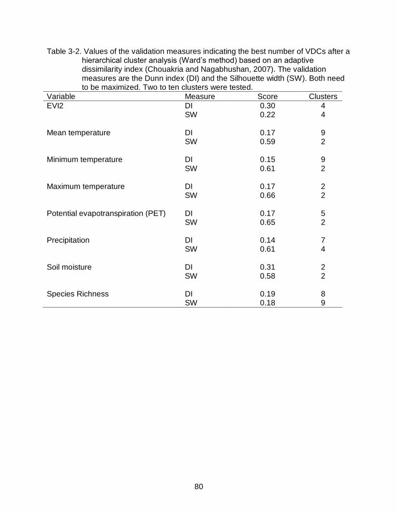
80
Table 3-2. Values of the validation measures indicating the best number of VDCs after a hierarchical cluster analysis (Ward’s method) based on an adaptive dissimilarity index (Chouakria and Nagabhushan, 2007). The validation measures are the Dunn index (DI) and the Silhouette width (SW). Both need to be maximized. Two to ten clusters were tested.
Variable Measure Score Clusters
EVI2 DI 0.30 4 SW 0.22 4 Mean temperature DI 0.17 9 SW 0.59 2 Minimum temperature DI 0.15 9 SW 0.61 2 Maximum temperature DI 0.17 2 SW 0.66 2 Potential evapotranspiration (PET) DI 0.17 5 SW 0.65 2 Precipitation DI 0.14 7 SW 0.61 4 Soil moisture DI 0.31 2 SW 0.58 2 Species Richness DI 0.19 8 SW 0.18 9

81
Figure 3-1. Average values of EVI2 and biophysical variables per community for the period 1987-2009. a) EVI2, b)
potential evapotranspiration, c) species richness, d) average temperature, e) minimum temperature, f) maximum temperature, g) precipitation and h) soil moisture.

82
Figure 3-1. Continued.
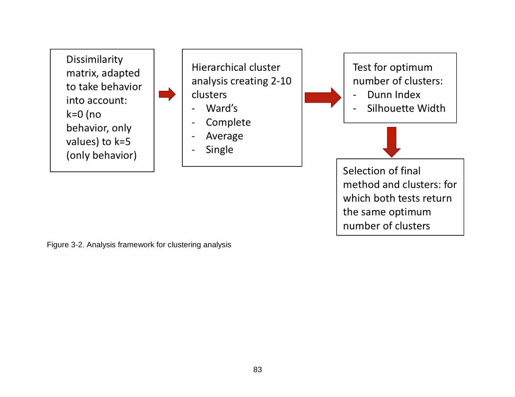
83
Figure 3-2. Analysis framework for clustering analysis

84
Figure 3-3. Selection criteria for determination of the appropriate number of clusters. These results are for clustering with Ward’s method with 𝑘 = 2 in the
calculation of the dissimilarity matrix. A) Results from the Dunn Index. B) Results from the Silhouette Width.

85
Figure 3-4. Dendrogram of EVI2 time series clusters, with 4 clusters selected.
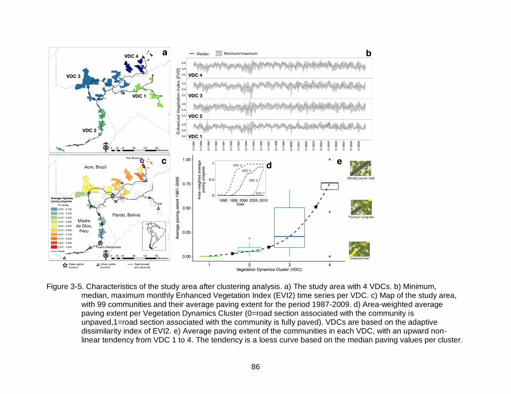
86
Figure 3-5. Characteristics of the study area after clustering analysis. a) The study area with 4 VDCs. b) Minimum,
median, maximum monthly Enhanced Vegetation Index (EVI2) time series per VDC. c) Map of the study area, with 99 communities and their average paving extent for the period 1987-2009. d) Area-weighted average paving extent per Vegetation Dynamics Cluster (0=road section associated with the community is unpaved,1=road section associated with the community is fully paved). VDCs are based on the adaptive dissimilarity index of EVI2. e) Average paving extent of the communities in each VDC, with an upward non-linear tendency from VDC 1 to 4. The tendency is a loess curve based on the median paving values per cluster.

87
Figure 3-6. Results from the breakpoint analysis of EVI2 per cluster. Panels on the left show the states over a moving window of 5 years. States are peaks in the probability distribution of values. Panels on the right show the F-statistic for the test of different means before and after a moving breakpoint, as well as the critical F-value, the breakpoint (black) and the point where road paving was at 10% in the cluster.

88
CHAPTER 4 CHANGING LANES: HIGHWAY PAVING IN THE SOUTHWESTERN AMAZON ALTERS LONG-TERM TRENDS AND DRIVERS OF REGIONAL VEGETATION
DYNAMICS
Background
The Amazon region in South America holds the largest areas of intact forest in
the world (Killeen and Solorzano, 2008);,(Keller, 2009), which is of great importance to
the global and regional climate system, biodiversity and carbon sequestration (Foley et
al., 2007; Myers et al., 2000). There is great concern about changes in land cover in the
Amazon, and the global and local consequences of such changes (Foley et al.,
2007);,(Davidson et al., 2012; Nobre and Borma, 2009) Anthropogenic disturbances
have direct impacts on forest cover by deforestation, and on forest structure and
composition that vary with the extent and frequency of the disturbances. For example,
logging and fire result in structural and phenological changes like reduction in basal
area, vegetation composition (J. Zhu et al., 2007), understory composition and vine
cover (Felton et al., 2006). Degradation of healthy forest reduces local, regional and
global ecosystem services (Foley et al., 2007).
Road construction and paving have been found to be a main driver of
deforestation (Laurance et al., 2009; 2002a; Marsik et al., 2011; Nepstad et al., 2001).
Large infrastructure projects also cause land degradation, impacts on abiotic processes
(such as hydrology), disruption of movement of organisms and increased mortality,
alteration of natural disturbance regimes (e.g. fire), and pollution. While infrastructure
has been demonstrated to bring socio-economic benefits, it can also lead to violent
conflict over natural resources, and rural-urban migration (Coffin, 2007; Laurance et al.,
2009; 2002b; Perz et al., 2011b; 2011a). Increasing interest in the relationships

89
between infrastructure development and the environment has given rise to the field of
‘road ecology’ (Forman, 2003), mostly focused on effects in the vicinity of roads. Most
studies have considered straightforward direct impacts such as deforestation (Laurance
et al., 2002a; Marsik et al., 2011), and localized impacts such as edge effects on
vegetation (Coffin, 2007; Lugo and Gucinski, 2000; Mesquita et al., 1999);,(Laurance et
al., 2009). For example, environmental impact assessments conducted for Amazonian
highway construction in Brazil only considered very limited areas of impact along the
roads, neglecting the potential regional impacts of road construction(Laurance et al.,
2009), such as forest degradation and changing vegetation dynamics in larger areas.
Vegetation dynamics refer to temporal fluctuations and spatial variability in vegetation
structure associated with disturbance regimes resulting from natural and anthropogenic
drivers. Changes in vegetation dynamics are indicative of the shifting forest structure
and the corresponding ecosystem services, which have social as well as ecological
impacts(Foley et al., 2007). It is therefore important to study changes beyond forest
cover changes, and to do an analysis that addresses both natural and human
processes, thus considering the system from a socio-ecological perspective.
The tri-national area in the southwestern Amazon (the so-called MAP area after
the provinces of Madre de Dios (Peru), Acre (Brazil) and Pando (Bolivia)) has been
characterized as a “biodiversity hotspot” (Killeen and Solorzano, 2008; Myers et al.,
2000; Perz et al., 2011a) where livelihoods are closely associated with natural
resources. The area is thus a useful example of a complex socio-ecological or coupled
natural-human system (Perz et al., 2011b; 2011a; 2013b). This means that disturbances
to the system can result from natural and anthropogenic drivers and their interactions
90
(Chazdon, 2003; Cumming et al., 2012; Davidson et al., 2012; Phillips et al., 2008). One
very specific anthropogenic disturbance in MAP is the development of roads, which has
been an important part of regional economic integration and development in recent
decades (Perz et al., 2008; 2011a; 2007). In particular, the Inter-Oceanic Highway
(IOH), connecting the Atlantic and Pacific Oceans and traversing the MAP region, is one
of the key infrastructure projects of the Peru-Brazil-Bolivia axis of integration (Rapp,
2005). The road is a major part of the Initiative for the Integration of Regional
Infrastructure in South America (IIRSA) that targeted infrastructure investments for
“strategic growth corridors for regional commerce” (Perz et al., 2011b).
Previous research found that even limited logging disturbances, without
significant forest cover loss, had a permanent local effect on forest structure in
Madagascar(Brown and Gurevitch, 2004). Differences in vegetation structure and
phenology between natural and anthropogenic treefall gaps 1 to 4 years after logging
were also identified in a Bolivian forest, despite almost identical forest cover
percentages (mean 88% for the anthropogenic gaps, and 91% for the natural gaps),
with lower mean number of flowering and fruiting plants in anthropogenic gaps, as well
as more regeneration of non-commercial pioneer species in these gaps(Felton et al.,
2006). A review study concluded that in Neotropical secondary forests, the recovery
trajectory of vegetation and its characteristics is uncertain in anthropogenic settings,
and dependent on site-specific factors and land use(Guariguata and Ostertag, 2001).
Changes in forest structure will in turn impact ecosystem service provision: changes in
tropical forest structure have been linked to modifications in wildlife populations in
Panama(DeWalt et al., 2003), and ecosystem productivity was found to be driven by

91
canopy phenology in the Amazon(Restrepo-Coupe et al., 2013). A forest inventory
study in the MAP region(Baraloto et al., 2015) found differences in forest value (based
on biodiversity, carbon stocks and timber and non-timber forest products) across the
frontier, and highlighted that deforestation and degradation do not always respond
similarly to road paving. Unfortunately, in situ vegetation structure assessments, while
extremely valuable for purposes of biodiversity valuation, are time-intensive, limited to
discrete locations and usually have a limited time dimension (synaptic), making it
difficult to assess changes in vegetation dynamics over time and space for a large area.
There is a need to comprehensively assess spatially distributed changes in vegetation
dynamics due to road paving to gain a better understanding of the system-wide effects
of infrastructure development.
Based on this evidence, we formulate a hypothesis that even if forest cover is
maintained, the structure of the forest will be regionally impacted in the presence of
advancing road paving. Our hypothesis asserts that there are different forest structures
and dynamics across a gradient of road paving, from dirt road to fully paved. Further we
suggest that forest change responds to different drivers as one moves along the paving
gradient. Specifically, anthropogenic covariates are expected to become more important
under more advanced paving conditions associated with increased regional
disturbances which are integral to driving and changing vegetation structure (Sousa,
1984; Thonicke et al., 2001).
To test this hypothesis, we require a long-term time series of vegetation index
values in order to study changes in vegetation structure and dynamics. The long-term
monthly Enhanced Vegetation Index (EVI), a remote sensing product from the Moderate

92
Resolution Imaging Spectroradiometer (MODIS), has been found to indicate vegetation
phenology and structure (Asner et al., 2000; Huete et al., 2002). It has been used in
previous studies to evaluate phenology, structure and ecosystem functioning (Bradley
and Fleishman, 2008; Cabello et al., 2012; Reed et al., 1994; Volante et al., 2012).
EVI2, used in this study, is a relatively new product (Z. Jiang et al., 2008), consisting of
EVI extended back in time from two-band Advanced Very High Resolution Radiometer
(AVHRR) data (1982-1999) and three-band MODIS EVI (2000 and after).
We combine the EVI2 data on forest vegetation with field-based socioeconomic
and biophysical data, which serve as indicators of drivers of vegetation change. Socio-
ecological survey data for the period 1987 – 2009 are available for 99 areas defined as
communities in the MAP region (Perz et al., 2011b; 2011a), as well as biophysical
covariates (see Methods). Paving of the IOH started at different times in different
countries across the MAP frontier, offering a valuable long-term study site with a paving
gradient (before, during and after) for road construction.
The objective of this paper is to test our hypotheses by applying advanced
statistical time series analyses to explore the structural and phenological changes of
forests at a regional scale, and how they are associated with the progression of road
paving and natural and human drivers and interactions. The time- and resource-
intensive methods that we apply allow us to analyse 99 unique long-term time series of
vegetation dynamics, without having to resort to simplification techniques. They focus
on finding shared variance and common trends across large numbers of time series.
We first identify areas of shared spatio-temporal vegetation dynamics along a road
paving gradient by means of cluster analysis. To identify common drivers for these
93
vegetation dynamics, we separate and attribute the relative importance of latent effects
(unexplained shared variance or trends) and explanatory natural and human covariates
(explained variance or direct effects) by means of Dynamic Factor Analysis (DFA), a
specialized dimension-reduction time-series analysis technique (Campo-Bescós et al.,
2013; Kaplan et al., 2010; Kuo and Lin, 2010; Ritter and Muñoz-Carpena, 2013a). The
results are twofold: identification of common trends and covariates across a larger
region, while also specifying their importance at local level. The objectives are twofold:
identification of common trends and covariates across a larger region, while also
specifying their importance at local level. Our innovative approach provides a way for
systematic and continuous assessment of forest degradation, represented by the shift in
the importance of trends and human and natural covariates under increased highway
paving.
Results
Identification of Clusters Vegetation Dynamics and their Association with Road Paving Extent
The socioeconomic survey includes 99 distinct communities in the MAP area in
the Southwestern Amazon (Figure 4-1a and Table A-1). Monthly time series of the
vegetation index, EVI2 (Z. Jiang et al., 2008)), for these communities were available,
with biophysical and socio-economic data (see Table 4-1). Hierarchical cluster analysis
on an adaptive dissimilarity index (Chouakria and Nagabhushan, 2007) of normalized
monthly EVI2 time series (1987-2009) permitted organization of the communities into 4
distinct clusters, based on identical Silhouette width and Dunn index results (Brock et
al., 2008), see Figures 3-3 and 3-4. These will be referred to as Vegetation Dynamics
Clusters (VDCs) in this study (Figure 4-1d). Characteristics of the EVI2 time series of

94
each VDC are given in Figure 4-1e and Table 4-1. Normalized values were used in this
study to retain the focus on the time series dynamics, and facilitate interpretation of
model results.
A distinct relationship was identified between VDCs (Figure 4-1c) and median
area-weighted average paving extent per VDC (Figure 4-1b). Road paving extent is
indicated by values between 0 and 1, with 0 indicating an unpaved road, 1 a fully paved
road, and anything in between indicating road paving in progress. An average was
taken for each community for the period January 1987 to December 2009, and is an
expression of when paving started and the length of the construction period (Figure 4-
1c). Thus, VDC 1 represents the unpaved system state, VDC 2 and VDC 3 transition
states, and VDC 4 the mostly paved system state. Subsequent models and analyses
were conducted for each VDC.
Common Trends Explain the Shared Variability of Each VDC
Dynamic Factor Models (DFMs) for VDCs 1 through 4 simulated EVI2 with
common trends only (DFMs I) identified 4, 7, 6 and 3 trends, respectively (Table 4-2),
based on their lowest Bayesian Information Criterion (BIC). The median goodness-of-fit
(Nash-Sutcliffe coefficient, Ceff) ranged between 0.67 and 0.76, indicating that the
models captured the shared variability within regions well. Respectively, 83%, 75%,
81% and 71% of VDC 1 through 4 models for each community had an acceptable(Ritter
and Muñoz-Carpena, 2013a) Ceff>0.60 (See Table A-6 for details and Figure A-1 for
examples of fitted time series). Overall, 98% of Ceff were higher than 0.50 (97 out of 99),
which is considered a good overall fit considering the typical noisiness of ecological
data. The analysis identified regional, shared variance – common trends – underlying
the vegetation dynamics for each VDC. Based on this result, we developed DFMs with

95
both trends and area-weighted averaged covariates to attempt to explain the shared
variance in each VDC (see Methods and Figure 4-7).
In a Disturbed System State, Covariates Explain More of the Variance In Vegetation Dynamics Than in an Undisturbed System State
Next, ‘DFM II’ (with covariates) for each VDC were obtained by stepwise
backward elimination of covariates or trends until the lowest BIC was reached. We
started with all covariates and the number of trends from DFMs I. Elimination was based
on the average importance of each model component per VDC, which was determined
with a computationally intensive method (Grömping, 2006) that calculates semi-partial
R2 of model components, averaged over all possible model orders (see Methods for a
detailed explanation of this measure of importance of regression components). This
produces an index of importance for each covariate for each community, which are then
averaged over the whole VDC to select the least important model component which will
be eliminated from the model. Some covariates were lagged before DFA application,
based on their cross-correlation with average area-weighted EVI2, to account for
delayed responses of vegetation dynamics to covariates (Table A-4). Table 4-2 lists
results for DFMs II with covariates ordered according to average importance for each
model (see Table A-7 for more detailed results). We found that each final DFM II (bold
in Table 4-2) based on the same number of trends as DFM I, with 6 to 8 covariates
each. Each DFM II contained both natural and human covariates. The models’ Ceff
stayed the same or increased: thus, while the number of trends remained the same,
their importance became smaller. A portion of the explained variance was shifted to the
covariates, while maintaining model fit. Again, for 98% of DFMs II, Ceff 0.50. Figure 4-
2a plots the total explained variance (R2), and Figure 4-2b shows the cumulative
³

96
importance of all trends and covariates compared to average paving extent in
communities. Importance is expressed as the average explained variance. While total
R2 stays fairly constant across all average paving extent (Figure 4-2a), the Loess curves
in Figure 4-2b show that once average paving extent passes 0.50 (50%), the
importance of trends and covariates shifts. Specifically, covariates explained
approximately 25% of variance under unpaved conditions, and 50% under paved
conditions, while trends exhibit a decrease their explanatory power. This implies that for
communities where paving started longer ago, much of the vegetation dynamics can be
explained with covariates directly. Tables A-8 to A-11 contain details on covariate time
series, model fits and weighting and loading coefficients for each community.
Variables Associated with Anthropogenic Activity Increase in Importance in Explaining Vegetation Dynamics in the Disturbed System State
In Figure 4-2c, the explained variance is subdivided into that associated with
natural covariates and with human covariates (Table 4-1). Communities with more
recent road paving (low average road paving extent, 0.10) showed an increase in
variance explained by human covariates compared to communities with no road paving
at all, but this decreased for communities with higher average road paving (0.25),
potentially due to adaptation of the system to a different disturbance regime. Eventually
though, there was an inversion of importance of natural and human covariates that
occurred after paving extent reached the 0.50 point.
Figure 4-3 shows that travel time to market, family density and enforcement of
tenure rules were the most important (highest average semi-partial R2) human
covariates in the DFMs II. The covariate time series used in the DFM IIs for each VDC
are shown in Figure 4-4. The standardized regression coefficients (β) of the DFMs give

97
additional information beyond the explained variance as its sign indicates an inverse or
reinforcing effect of the covariates on vegetation dynamics. For interpretation of the
coefficients of this study, we need to keep in mind that covariates were added to the
models with lags (Figure 4-5). The inverse effect of family density is intuitive: increasing
family density (Figure 4-4) leading to decreasing EVI2 could be linked to increased
pressure on vegetation and forest exploitation.
For travel time to market, we need to take into account the average paving extent
of communities in each VDC to understand its effect: for later paved communities (low
average paving extent, VDC 2), the decrease in travel time is associated with
decreased EVI2 (positive β), again due to increased pressure and exploitation
associated with better access to markets for locals and better access to forest products
by outsiders. However, for communities that had paved roads earlier in the study period
(higher average paving extent, VDC 4), the sign of β reverses to negative values. The
change in travel time is less pronounced and occurs over a longer time period (Figure 4-
4), so it is possible that over time communities shift their focus to more urban sources of
income rather than forest-based ones, prompting higher EVI2 over time.
Enforcement of tenure rules on deforestation also had a positive effect on EVI2 in
communities that had unpaved roads during the study period (VDC 1), as expected.
While enforcement also increased for the communities that had paving longer, in VDC 4
(Figure 4-4) its effects appeared negative (i.e. lower EVI2). A possible explanation for
this seemingly counterintuitive result is the 13-month lag applied to this covariate (in
Figure 4-5 the lags are given above each covariate plot), relevant mostly to Acre, Brazil
(Figure 4-1d). Most of the enforcement change occurs in the early years (1990-1991,

98
Figure 4-4), after which enforcement stays fairly constant. Extraction of forest resources
and conversion to agriculture had been going on for many decades in this area, and in
the 1980s several groups (ranchers, rubber tappers, colonists) clashed over land use
and deforestation (Hoelle, 2011). Subsequent increased enforcement might have been
too late to affect vegetation positively.
Among Natural Covariates, Temperature is the Main Direct Driver of Vegetation Dynamics
Temperature time series were important factors in all VDCs. Normalized
minimum, maximum and average temperature had different temporal patterns (Figure 4-
4) and combined appeared relevant in simulating vegetation dynamics (Figure 4-3): on
average, across all communities, the variance explained by the three temperature time
series (average semi-partial R2) is 32% of all variance explained by natural covariates.
This is probably due to their effect on photosynthesis, which affects phenological
signatures. Figure 4-3 shows that with increased average paving, maximum
temperature becomes relatively more important than minimum and average
temperature. Minimum temperature is used unlagged in the models, indicating an
immediate effect of this covariate in the simulation; average and maximum
temperatures are lagged respectively 12-13 and 13-14 months (Figure 4-5). Maximum
and average temperature have an effect on germination, flowering or other reproductive
processes, which would explain the longer lag in its effect. The positive β coefficients for
temperature shows that temperature and vegetation dynamics are similar (increased
temperature simulates increased EVI2 and vice versa), which is expected in this study
area. Climate change is projected to affect maximum temperatures significantly in the

99
future, including its anomalies (Pachauri et al., 2015), indicating that areas under the
influence of road paving disturbances will be sensitive to these changes.
In terms of hydrological controls, precipitation itself is less important than
potential evapotranspiration and soil moisture in the models (Figure 4-3). Their
importance decreases in areas with higher average road paving extent. The importance
of soil moisture for VDC 1, VDC 2 and VDC 3 is supported by previous research
(Quesada et al., 2012) which pointed to the relevance of the hydrologic cycle in
combination with soil properties in these areas with mostly natural disturbances and
limited anthropogenic disturbances. In terms of the effect of soil moisture (the β
coefficient), it is mixed when there is less road paving (Figure 4-5). As road paving
increases, it becomes more distinctly negative (-0.40 < β < 0.0), meaning lower soil
moisture leads to a higher EVI2. A key component in interpreting this result is the lag of
3-4 months applied to this covariate. While soil moisture usually peaks at the beginning
of the year during the later portion of the wet season (March-April), EVI2 generally
reaches its lowest points around the middle of the year during the dry season (June-
September). By implementing the soil moisture with a lag, EVI2 and soil moisture
essentially display opposite dynamics, and the timing of soil moisture peaks and lows
become a factor in simulating EVI2 lows and peaks for most communities. However,
some communities with lower average paving extent have a positive β coefficient (0.0 <
β < 0.3): for VDC 1, for which soil moisture was also lagged 3 months, this implies that
EVI2 in these areas have later peaks and dips than the other areas – probably because
of different vegetation types and/or structure. For VDC 2, the lag of 10 months plays a
role in β coefficients being positive: soil moisture peaks are now aligned with EVI2
100
peaks in December-January. Overall, soil moisture dynamics appear to be an important
control in vegetation dynamics, but this relevance disappears when average road
paving increases.
While the importance of potential evapotranspiration is fairly constant across
communities (Figure 4-3), the β coefficient is negative for a number of communities in a
transition paving state (Figure 4-5) until the most paved state, where potential
evapotranspiration has a positive effect on EVI2. The early negative effect indicates that
higher evapotranspiration results in lower EVI2. This is counterintuitive since we would
expect a positive effect: higher evapotranspiration signifies more photosynthetic activity
and thus higher EVI2 values. A component to consider is that potential
evapotranspiration is lagged. The lag is 14 months, meaning the PET peak of
August/September is aligned with October/November EVI2 values, and the lowest PET
values for July with September EVI2 values. EVI2 generally rises after the dry winter
period (May-September, Supplementary Fig. S1), but the timing of this rise varies
across the study area between September and November, and sometimes even
December or January. There is similar variation in the beginning of the year, when
potential evapotranspiration starts dropping (it is based mostly on temperature, see
Methods), but EVI2 can still stay high. These differences in phenological signature could
contribute to negative β coefficients. Since PET dynamics are fairly consistent (Figure 4-
4), this points to mixed vegetation dynamics during the (early) transition state.
The negative coefficients for species richness (Figure 4-5) for some communities
are similar to earlier findings (Baraloto et al., 2014), which established that there are
trade-offs between plant diversity and forest structure covariates in the region.

101
Increased forest structure (in terms of aboveground biomass) was associated with less
diversity. The species richness time series included in the models showed no clear
positive or negative trend for these areas. The percentage of a community under forest
cover predictably has a positive β coefficient (Figure 4-5), but only plays a role in VDC 1
(Figure 4-3 and 4-5), the communities with no paving.
Low Frequency Signals Explain Trend Behavior Across the Study Area as a Whole, but Dominate Particularly in the Paved State
While the number of common trends stays the same for each VDC for Models I
and II (Table 4-1), their importance in explaining variance is diminished for all VDCs
once covariates are added in Models II, compared to Models I. None of the R2 values
for the Models II has decreased in comparison with Model I (Figure 4-2a), but the
covariates now also explain variance in all communities (Figure 4-2c). This is a sign that
the effects of certain covariates on vegetation dynamics were present in those trends,
and were now removed from the trends. The remaining trends still explain a fair amount
of the variance across all VDCs (25-50%). These could represent covariates missing
from the models (e.g. fire occurrence, actual evapotranspiration, climate indices), or
non-linear interactions between covariates that are not modeled explicitly with DFA.
The variance explained by the trends for each community (expressed as average
semi-partial R2) is plotted in Figure 4-6a, with the trends over time shown in Figure 4-6b.
It is of interest to note that even for communities with a similar paving history (x-axis for
Figure 4-6a), there is a range in the amount variance explained by each trend across
communities. In Figure 4-6a, it is easiest to see for the first trend in each VDC due to
the color scheme, but the other trends also vary in the variance they explain. This is a

102
clear sign that there is information contained in the trends that is spatially variable and
not included elsewhere.
If time series of physical processes are (partially) a result of the sum of various
frequencies(Koopmans, 1995), spectral analysis can help disentangle them.
Frequencies (i.e. cycle lengths) with the highest power spectral density contribute most
to explaining variance in relative terms (this method does not quantify absolute
contribution). The spectral power density of signals contained in the trends was
determined (see Methods), and for each trend the three signals with the highest density
are visualized in Figure 4-6c. Certain low-frequency signals – long cycle lengths - show
up consistently in each region, and we attribute these to solar and climatic influences.
Solar activity and its associated radiation have an influence on the earth’s biosphere
(Brajša et al., 2009; Offermann et al., 2010) and its variation is acknowledged as a
natural climate forcing (Pachauri et al., 2015). The solar cycle has an 11- to 22-year
frequency, and a 5.6-year periodicity has been shown to be significantly present too
(Ramanuja Rao, 1973). Frequencies of 22.5, 11.25 and 5.625 years are present in the
trends in this study. The Pacific Decadal Oscillation (PDO), a pattern of ocean-
atmosphere variability, has been found to play a role in the Amazon in previous
studies(Arias et al., 2010; Herzog et al., 2011; G. A. M. D. Silva et al., 2011). The PDO
contains a 4.8- and 8-year frequency (Table A-11), close to the 4.5- and 7.5-year
frequencies also found in a number of the DFM trends.
There is a decrease in higher frequency signals (cycle lengths < 18 months)
across the VDCs with increased paving extent (Figure 4-6c). Especially for VDC 4, more
of the variance of the trends is captured in the low frequency signals. Since the trends

103
explain relatively little of the overall EVI2 variance for this VDC (Figure 4-6a), we
deduce that the covariates included in the model that offer high frequency variations
(temperature, precipitation, PET) have more explanatory power on vegetation dynamics
in this VDC.
Unpaved to Paved Conditions Represent Two Stable System States with a Transition State in Between Them
A transition state between paved and unpaved conditions can be clearly
identified in Figures 4-2b and 4-2c. There is a shift in the importance of trends and
covariates explaining EVI2 dynamics, as well as a shift in importance between natural
and human covariates, as was noted above. Both these shifts happen around an
average paving extent of 0.75. This is an interesting finding as it shows that this system
took more or less 16-17 years (0.75 of the 22-year study period) to go through an
assumed full transition after road paving.
The number of trends in the paved and unpaved state is similar and low (Figures
4-6a and 4-6b). This points to the uniformity of vegetation dynamics in the communities
across these regions – possibly because the dynamics reached a stable state
considering the duration they were unpaved or partially paved. The transition states,
with 6 and 7 trends, have more heterogeneity in paving and impacts across the
communities in their regions and a variety of vegetation responses. This highlights that
while paving is ongoing, changes and system states at a regional level are more
heterogeneous and more difficult to predict. Once the system stabilizes again, the
system state is different than before the disturbance: this is visible, in addition to DFM
specification in terms of covariates, in the frequencies contained in the trends. That

104
VDC4 is stable is an assumption: re-analysis of longer time series in the future would
have to confirm this.
Discussion
Main Findings
This research offers support for the hypothesis that there are areas that have
distinct forest structures and phenologies along a road paving gradient, and provides
support for the second part of the hypothesis, that different covariates and mechanisms
drive vegetation dynamics across the road paving gradient.
We have found distinct areas with common temporal vegetation dynamics
(VDCs), associated with road paving progression in the SW Amazon, confirming our
hypothesis that vegetation structure is altered with increased road paving. With a time
series dimension reduction technique, Dynamic Factor Analysis (DFA), we uncovered
common trends and a number of (lagged) socio-economic and biophysical covariates
that explain shared variance of EVI2 for each VDC. We found differences in the
Dynamic Factor Models (DFMs) between VDCs in terms of covariates and trends
included, their importance in explaining variance, and 𝛽 coefficients (negative or positive
effects). There are two stable system states identified with unpaved and paved
conditions (VDC 1 and VDC 4). These two stable states have distinct differences in
human and natural driving factors of vegetation dynamics. Human covariates are
relatively more important in the paved state (family density and travel time to markets);
similarly, the natural covariate for temperature is important in the paved state. In the
unpaved state and the transition states, there is considerable influence from natural
variables like potential evapotranspiration, soil moisture, and minimum and average
temperatures. Lastly, results show there is a change in trends from the unpaved to the

105
paved system state, with trends losing both importance and overall number of signals,
notably high-frequency signals. The latter is associated with covariates explaining more
variance in the paved state directly. Within VDCs, for communities with similar average
paving extent, trends vary in their contribution to explained variance. This suggests that
there are covariates with spatial variation that have not been included in this study, but
that these are less important for the paved state (VDC 4).
Broader Impacts
This study has shown the power of Dynamic Factor Analysis when applied to a
complex data set where time series are subject to change over an extended period of
time and space. This offered a continuous overview of the dynamics in the importance
of the effects of different covariates, as opposed to snapshots in time. DFA provides a
systematic framework to study how forest degradation evolves over time as a process
like road paving unfolds. Other areas in which this method could prove useful are
experimental interventions in biological and health fields, to assess how complex
systems respond, or governmental regulations affect the outcome.
The results of the study will benefit local and regional planners, as well as
conservation initiatives at a practical level. The findings shed light on which covariates
are relevant at different phases of the road paving process as they impact regional
vegetation structure. The results thus point to management options by identifying
important covariates that can also be managed, such as enforcement of tenure rules
and migration. The analysis also provides insights into which biophysical covariates
affected by climate change will have the most impact and where. With temperature
anomalies projected to change in the future(Pachauri et al., 2015), the effect on areas in
a paved state will be stronger. Most importantly though, the study indicates that

106
vegetation dynamics - and their effects on ecosystem services - will differ across
regions associated with different levels of road paving. Future research on specific
ecosystem services changes with change in forest dynamics is relevant for both
conservation as well as future economic opportunities in the study area. Many
livelihoods are strongly dependent on the natural environment, and infrastructure
planning initiatives should anticipate these effects. Provisions should be made in the
planning stages of a road project to monitor vegetation dynamics after project
completion, beyond only deforestation. More detailed and localized technologies, such
as Light Detection And Ranging (LiDAR) or products from the Fluorescence Explorer
(FLEX), will provide useful. Governments and research institutes should invest in these
technologies for ongoing monitoring.
Lastly, this study adds a regional, up-scaled analysis to the field of road ecology.
As the people’s desire for development, trade and connections continues, road paving
will undoubtedly continue into many forested areas such as the Amazon, Central Africa
and Southeast Asia with unparalleled ecosystem services provision(Laurance et al.,
2014).
Limitations and Further Research
While remote sensing products are increasingly available and useful for doing
larger-scale regional analyses, inherent noise in the data should be carefully evaluated.
This is especially true in humid tropical regions, which exhibit extended periods of cloud
cover contributing to observation error. While the models exhibit an acceptable
goodness-of-fit for most communities, their performance is low in some areas partly due
to observation error. Further research on signals and frequencies in EVI2 data would be
beneficial to quantify differing vegetation dynamics in more detail and assess errors, as

107
well as field studies that measure biomass and vegetation structure, or more detailed
remote sensing studies (e.g. with LiDAR).
While DFA is efficient at capturing variance in ecological time series because of
its autoregressive approach to modeling trends, if the variance is not accounted for
among the covariates in expanded models and instead remains captured in the trends,
it stays unknown. This requires more detailed investigations into issues such as logging,
the role of fire, and species composition in terms of functional groups. It is however
challenging to obtain reliable data on these concepts for sufficiently long periods of time.
Dynamic Factor Models add covariates linearly, and while possible lagged
responses have been accounted for, interactions are not explicitly accounted for. Future
research should focus on untangling interactions between both human and natural
covariates, in particular with mechanistic models. This would also assist in identifying
causal relationships, since DFA does not account for this.
Methods
Study Area
The 99 communities included in this study lie within the states of Madre de Dios
(Peru), Acre (Brazil) and Pando (Bolivia), also referred to as the “MAP” region. The area
lies between 9°48’ S and 13°1’ S latitude and 67°10’ and 70°31’ W longitude, at the foot
of the Andes Mountains and in the headwaters of tributaries of the Amazon River. The
climate is tropical, classified as Awi (Köppen climate classification), with an average
daily temperature of 25° C and mean annual precipitation of approximately 2000 mm.
The dry season runs from June to October, in which monthly rainfall averages < 100
mm. The types of forest in the area are dense tropical forest, open tropical forest with
palm trees, and open forests dominated by bamboo – with many locations containing a

108
mix of these forest types (Carvalho et al., 2013; Rockwell et al., 2014; Salimon et al.,
2011).
The Inter-Oceanic Highway was paved between approximately 1992 (Rio
Branco) and 2010 (Peru). Communities in Bolivia still had unpaved roads during the
time period studied since road paving had not progressed much further than Cobija
(Figure 4-1a). These are resource-dependent rural communities that were part of earlier
studies (Perz et al., 2013b; 2011b; 2011a). They are defined as being “distinct land
tenure units and/or population centers” (Perz et al., 2011a). Population densities are
low, with an average family density of 0.07 families/km2 and a maximum of 3.17
families/km2 for the study period. Land use is described as complex and shifting, and
includes urban areas, subsistence agriculture, logging, gold mining, conservation areas,
secondary forest and old-growth forest in which non-timber forest products (NTFPs
such as brazil nuts and rubber) are harvested (Phillips et al., 2006).
The methodologies that were applied to clean and analyze data are depicted in
Figure 4-7.
Response Covariate: Vegetation Dynamics, EVI2
Data for the enhanced vegetation index (EVI2) used in this analysis were
obtained from the University of Arizona’s Vegetation Index and Phenology (VIP) lab,
which applies an algorithm to translate two-band data from the Advanced Very High
Resolution Radiometer (AVHRR) into MODIS EVI (Z. Jiang et al., 2008). AVHRR data
have been collected since 1982. The data used in this analysis (1987-2009) were
obtained from the VIP lab in October 2013 in monthly time steps and at a 0.05°
resolution. Area-weighted time series were extracted for each community polygon.
109
Data correction was performed to address outliers and discrepancies between
AVHRR-derived EVI (1982-1999) and MODIS EVI (2000-2010), because AVHRR-
derived EVI exhibited consistently lower values (an overall average of 0.387 vs. 0.513).
This is attributed to the lower quality of AVHRR data in areas with high cloud density
(pers. comm. Dr. K. Didan).
The final data set generally has the lowest EVI2 occurring in the driest months
(June, July and August). EVI2 peaks during the wet season, in November, December
and January. Variations in monthly medians across communities are larger during the
wet season than the dry season (Figure 2-1).
Candidate Covariates Related to Human Activity
Annual data sets for a variety of covariates associated with human activity in the
study area are available from previous studies (Perz et al., 2013b). Variables uses in
this study are: number of families in a community (FAM), family density (FAMD, number
of families / km2), population in the nearest capital (PNC), population in the nearest
market (PNM), paving (PAV), deforestation allowed under tenure rules (TEN),
enforcement of tenure rules (ENF), travel time to the nearest capital (TTC) and travel
time to the nearest market (TTM). See Table A-2. Data sets were linearly interpolated to
create monthly time series.
PAV is a value between 0 and 1 representing proportion of a road segment
paved, and is derived from field work. The year when paving of the road segment along
which a community sits is finalized is taken as the starting point to estimate increments
in the proportion paved. If a community is along a highway segment between two towns
that was paved by 1999, that community gets a value of “1” for 1999 (and subsequent
years). Proportions paved in the years prior are derived from field notes with the timing

110
of the onset and conclusion of paving of that segment, with a linear interpolation of
paving proportions during the intervening time period.
Travel times, representing connectivity, are in minutes and based on the distance
to the nearest capital or market, and average travel speeds taking into account paved
and non-paved segments. For some communities, the nearest market is also the
capital, rendering the same time series for these covariates (Figure 4-1a).
TEN and ENF are similarly based on fieldwork, which included workshops with
stakeholders, and official rules for resource use given by governments. TEN is simply
the percentage of forest a community is allowed to cut down. Values vary between 0
and 1, representing 0 to 100% deforestation allowed. ENF are perceptions by experts
as to the extent to which those use rules are actually enforced by government agencies
responsible for oversight, which roughly corresponds to the probability of infractions
being detected and punished. Here again, the values run from 0 to 1, with higher values
indicating more likely enforcement.
Candidate Covariates Associated with Biophysical Processes
Monthly data sets were sourced in June 2013 from the Climatic Research Unit
(CRU) at the University of East Anglia. Covariates include the mean, minimum and
maximum temperatures, precipitation and potential evapotranspiration (AVET, MINT,
MAXT, P, PET). For more details, see Table A-2. The mean, minimum and maximum
temperatures (in °C) and precipitation (in mm) were obtained at a resolution of 0.5 x
0.5° (Harris et al., 2013), and were assigned to each community polygon in an area-
weighted manner. Potential evapotranspiration (in mm) is also included in the CRU data
set, and is calculated from a variant of the Penman-Monteith formula, using mean,

111
minimum and maximum temperature, vapor pressure and cloud cover (Harris et al.,
2013).
Soil moisture (SM) comes from the NOAA Climate Prediction Center (CPC)
model at a resolution of 0.5 x 0.5°, which uses CPC precipitation data and temperature
data from the NCEP/NCAR Reanalysis(Fan, 2004). The data are provided as average
soil moisture in terms of water height equivalents (mm). As with the other data sets, the
soil moisture data are calculated as an area-weighted time series for each community
polygon.
Forest area as a percentage of community polygon area (FOR) is sourced from a
deforestation study conducted in the area (Marsik et al., 2011). Forest and non-forest
percentages for each polygon are available for the years 1986, 1991, 1996, 2000, 2005
and 2010, and were interpolated to obtain monthly values.
Inferred species richness (SR) is alpha diversity computed from Landsat imagery
by applying a method that is based on the Shannon entropy of pixel intensity
(Convertino et al., 2012).
Clustering
To find the “optimum” number of clusters, 3 steps were implemented: 1)
calculation of a dissimilarity matrix, 2) application of Ward’s hierarchical clustering, and
3) calculation of the Dunn index and Silhouette width as measures of compactness and
separation of the clusters.
The EVI2 (1982-2010) was normalized and a time series-based dissimilarity
matrix D was established (Chouakria and Nagabhushan, 2007). D contains aspects of
Euclidian distance between time series, as well as a temporal correlation measure.
Therefore, the proximity measure is related to similarity of values and time series
112
behavior. Behavior is defined as the increase or decrease of values between points in
time, as well as the rate of this change. An automatic adaptive tuning function is
included in the conventional dissimilarity index calculations, with a parameter k that
determines how much behavior and value proximity contribute to D. At k=0, D is only
based on values, and at kmax = 5 behavior contributes most.
Ward’s hierarchical clustering was then applied to D to group communities
together. Ward’s method calculates the distance between clusters as the increase in the
sum of squares if they are merged. All series start out with the value zero, as they are
all regarded as their own cluster, and series or clusters are merged for those that have
the smallest distance increase. The Dunn index and Silhouette width are calculated for
2 to 10 clusters to determine the appropriate k and number of clusters. For k = 2 and 4
clusters, the Dunn index was highest (0.085) as well as the Silhouette width (0.36). All
candidate covariate time series were clustered according to the regions that resulted
from the EVI2 clustering analysis, to use in further analyses.
Lagging and Reduction of Covariate Data Set
All candidate covariate time series (1987-2009) were reduced to a single time
series for each VDC as an area-weighted average. Based on the highest statistically
significant cross-correlation with area-weighted EVI2 of its region, each regional
candidate covariate was lagged anywhere from 0 to 19 time steps (months); for more
details, see Table A-4. A Variation Inflation Factor (VIF) analysis was applied to detect
collinearity (VIF > 10) (Neter et al., 1996; Zuur et al., 2007), with covariates with the
highest VIF excluded from the data set in an iterative manner until a covariate data set
remained with all VIFs < 10 (see Table A-5).

113
Dynamic Factor Analysis
Dynamic Factor Analysis (DFA) is a dimension-reducing statistical analysis that
is applied to explore relationships between response covariates and common (shared)
covariates in dynamic systems over time. It aims to explain shared variation of observed
time series using a set of common trends, with the number of trends being substantially
smaller than the number of observed time series. These common trends across all time
series model temporal variation across the response covariates as linear combinations,
and represent driving factors across all time series. The coefficient associated with a
trend in a time series gives an indication of the importance of that trend for that time
series. The trends are estimated using an Expectation Maximization (EM) algorithm,
which allows maximum likelihood estimation in situations where there are latent random
covariates in a model (Holmes et al., 2014; Zuur et al., 2007; 2003a). Covariates can be
added to the model in a linear fashion. The Dynamic Factor Model being estimated is
𝑆𝑛(𝑡) = ∑ 𝛾𝑚,𝑛𝛼𝑚(𝑡)𝑀𝑚=1 + 𝜇𝑛(𝑡) + ∑ 𝛽𝑘,𝑛𝜈𝑘(𝑡) + 휀𝑛(𝑡)𝐾
𝑘=0 (4-1)
𝛼𝑚(𝑡) = 𝛼𝑚(𝑡 − 1) + 𝜂𝑚(𝑡) (4-2)
𝑆𝑛(𝑡) is the value of the n-th response covariate at time t; 𝛼𝑚(𝑡) is the m-th unknown
trend at time t; 𝛾𝑚,𝑛 represents the unknown factor loadings; 𝜇𝑛(𝑡) is the n-th constant
level parameter for displacing each linear combination of common trends up and down;
𝛽𝑘,𝑛 represents the unknown regression parameters for the K covariate time series
𝜈𝑘(𝑡); 휀𝑛(𝑡) and ηm(t) are the error components. 휀𝑛(𝑡) can be interpreted as the process
errors of the hidden trends, and 𝜂𝑚(𝑡) as the observation errors, which are independent
Gaussian noise with zero mean and a variance-covariance matrix that can take different
forms. For this analysis, the variance-covariance matrices are implemented as

114
symmetric (diagonal) matrices. The constant level parameter (𝜇𝑛(𝑡)) is set to zero since
normalized data are used.
The Dynamic Factor Models (DFMs) were assessed based on their goodness-of-
fit (Nash-Sutcliffe coefficient of efficiency, Ceff) and parsimony (Bayesian Information
Criterion, BIC). The aim throughout model development was to add enough covariates
to explain most of the shared variance across all response covariate time series, so that
reliance on the trends in minimized, without lowering the goodness-of-fit or worsening
model parsimony (Campo-Bescós et al., 2013; Kaplan et al., 2010; Kaplan and Muñoz-
Carpena, 2011; Kuo and Lin, 2010; Muñoz-Carpena et al., 2005; Ritter et al., 2009).
Whereas Models I contained only trends, Models II contained trends and
covariates. Models with lowest BICs were considered the best models. To find the best
Models II, a backwards elimination procedure was adopted where initial ‘full’ models
contained the number of common trends from the best Model I and all covariates. The
covariate or trend least important to explaining variance in the model was dropped, and
a new Model II was then developed with a reduced set of trends and covariates. This
step was iterated until the BIC hit its lowest point; covariate elimination was halted when
BIC started rising again.
Importance of Trends and Covariates
The importance of trends and covariates in the models was examined by
variance partitioning (Chevan and Sutherland, 1991; Johnson and Lebreton, 2004; Zuur
et al., 2007). This was implemented as the average semi-partial R2 over all possible
orders of model components, as well as its ‘relative importance’ (Grömping, 2006;
Lindeman et al., 1980). The latter is relative to the total coefficient of determination (R2),
is non-negative and the values for all model components add up to 1, or 100% of R2

115
(also known as the Lindeman, Merenda and Gold (LMG) method (Grömping, 2006)).
Since DFA estimated a unique DFM for each community, based on common trends and
covariates, we averaged the relative importance of each trend and covariate across the
VDC, to then eliminate the factor with the lowest average value.
This approach of taking the average semi-partial R2 over all possible orders of
model components is driven by the fact that the order in which non-orthogonal
regressors appear in the regression determines the amount of variance they explain –
which could lead to biased results if not all orders are taken into account.
Spectral Analysis of Trends
To gain insight in the periodic components of the trends, spectral analysis was
performed. Dominant periods or frequencies were identified by spectral density
estimation: higher values indicate relatively more importance of a particular frequency in
explaining oscillations in the trend. For each trend, the spectral density is estimated
using a fast Fourier transform with a modified Daniell kernel with dimension 2 as a
smoother, and the 3 frequencies with the highest density were selected for display in
Figure 4-6.
Software Used
All data cleaning was done in R (3.2.4) and Python. Maps were rendered in
ArcMap. R was used for all subsequent analyses and figures. The following packages
were used: TSclust (adaptive dissimilarity index), clValid (cluster validation, adjusted to
be able to work with the adaptive dissimilarity index as input), fmsb (VIF), MARSS
(DFA), relaimpo (relative importance in linear regressions), hydroGOF (Nash-Sutcliffe
coefficient), ggplot2, reshape2, zoo, grid, gridExtra, cowplot and gtable (figures).

116
Data Availability
The data sets generated during and/or analysed for this study are available in the
Figshare repository, 10.6084/m9.figshare.c.3858064.
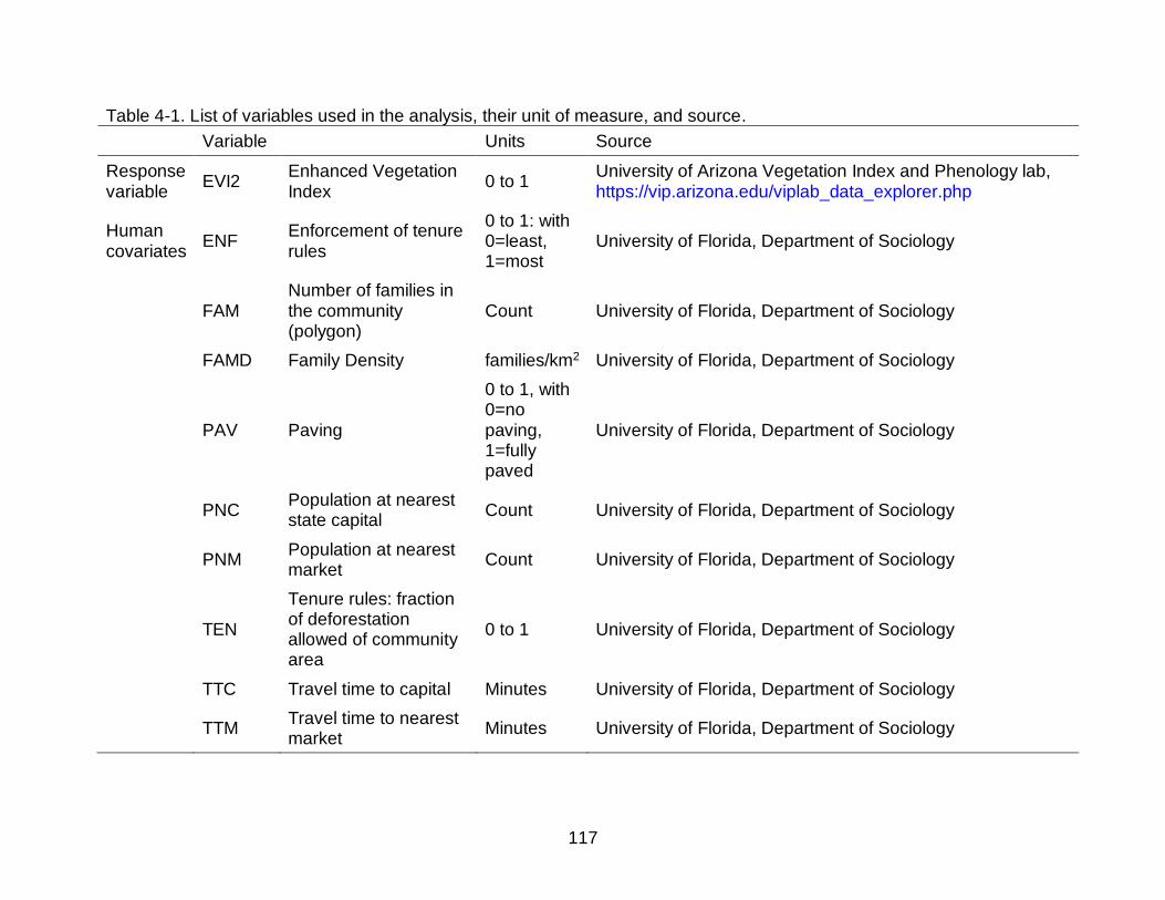
117
Table 4-1. List of variables used in the analysis, their unit of measure, and source.
Variable Units Source
Response variable
EVI2 Enhanced Vegetation Index
0 to 1 University of Arizona Vegetation Index and Phenology lab, https://vip.arizona.edu/viplab_data_explorer.php
Human covariates
ENF Enforcement of tenure rules
0 to 1: with 0=least, 1=most
University of Florida, Department of Sociology
FAM
Number of families in the community (polygon)
Count University of Florida, Department of Sociology
FAMD Family Density families/km2 University of Florida, Department of Sociology
PAV Paving
0 to 1, with 0=no paving, 1=fully paved
University of Florida, Department of Sociology
PNC
Population at nearest state capital
Count University of Florida, Department of Sociology
PNM
Population at nearest market
Count University of Florida, Department of Sociology
TEN
Tenure rules: fraction of deforestation allowed of community area
0 to 1 University of Florida, Department of Sociology
TTC Travel time to capital Minutes University of Florida, Department of Sociology
TTM
Travel time to nearest market
Minutes University of Florida, Department of Sociology

118
Table 4-1. Continued.
Variable Units Source
Natural covariates
AVET Mean temperature °C University of East Anglia, Climate Research Unit, https://crudata.uea.ac.uk/cru/data/hrg/
FOR Forest area
as fraction community area
University of Florida, Department of Geography
MAXT Maximum temperature °C
University of East Anglia, Climate Research Unit, https://crudata.uea.ac.uk/cru/data/hrg/
MINT Minimum temperature °C
University of East Anglia, Climate Research Unit, https://crudata.uea.ac.uk/cru/data/hrg/
P Precipitation mm
University of East Anglia, Climate Research Unit, https://crudata.uea.ac.uk/cru/data/hrg/
PET
Potential evapotranspiration
mm University of East Anglia, Climate Research Unit, https://crudata.uea.ac.uk/cru/data/hrg/
SM Soil moisture mm
NOAA Climate Prediction Center (PCP), https://www.esrl.noaa.gov/psd/data/gridded/data.cpcsoil.html
SR Species richness
Alpha diversity
University of Florida, Department of Agricultural and Biological Engineering

119
Table 4-2. Results of dynamic factor analyses of Enhanced Vegetation Index (EVI2) for 4 Vegetation Dynamics Areas (VDCs). Model I: only trends are fitted, no explanatory variables. Model II: both trends and explanatory variables (EV) are fitted. EVs are listed according to their relative importance (LMG) in each model. BIC is the Bayesian Information Criterion, Ceff is the Nash-Sutcliffe coefficient of efficiency. Model results in bold are the selected models for further discussion.
VDC Model Number of trends (γ)
Explanatory variables (EV) BIC Median Ceff
(95% confidence interval)
1 I 1 10205 0.54 (0.27-0.81) unpaved I 2 10011 0.62 (0.30-0.85) (n=18) I 3 9876 0.71 (0.32-0.87) I 4 9789 0.74 (0.49-0.87) I 5 9796 0.75 (0.50-0.89) II 4 ENF AVET MINT PET FOR SR SM FAMD MAXT P 9994 0.75 (0.52-0.87) II 4 ENF AVET MINT PET SR SM FOR MAXT FAMD 9958 0.75 (0.52-0.88) II 4 FOR ENF AVET MINT PET SR SM MAXT 9923 0.75 (0.51-0.87) II 4 FOR AVET MINT ENF PET SM SR 9896 0.75 (0.50-0.87) II 3 FOR AVET MINT SR PET ENF SM 9939 0.73 (0.40-0.86) 2 I 1 14379 0.41 (0.14-0.84) transition I 2 10915 0.49 (0.18-1.00) (n=24) I 3 10305 0.60 (0.24-1.00) I 4 10144 0.72 (0.29-1.00) I 5 10055 0.77 (0.39-1.00) I 6 10043 0.80 (0.48-1.00) I 7 10007 0.80 (0.51-1.00) I 8 10034 0.82 (0.53-1.00) II 7 TTM PAV PET SM MAXT P MINT AVET SR TEN 10390 0.83 (0.54-1.00) II 7 PAV TTM PET SR MAXT SM P MINT AVET 10323 0.83 (0.54-1.00) II 7 PAV TTM SR PET SM MAXT P MINT 10266 0.83 (0.54-1.00) II 7 PAV TTM PET SM MAXT P SR 10244 0.82 (0.53-1.00) II 7 PAV TTM PET SM MAXT SR 10262 0.83 (0.46-1.00)

120
Table 4-2. Continued
VDC Model Number of trends (γ)
Explanatory variables (EV) BIC Median Ceff
(95% confidence interval)
3 I 1 23129 0.63 (0.40-0.76) transition I 2 22261 0.66 (0.41-0.82) (n=43) I 3 21573 0.71 (0.48-0.85) I 4 21223 0.74 (0.55-0.90) I 5 18230 0.74 (0.55-1.00) I 6 18082 0.77 (0.56-1.00) I 7 18134 0.78 (0.56-1.00) II 6 PET SM MINT FAMD AVET MAXT P TEN SR ENF 19010 0.79 (0.59-1.00) II 6 PET MINT SM MAXT AVET FAMD P TEN SR 18900 0.79 (0.59-1.00) II 6 PET MINT SM MAXT AVET FAMD P TEN 18817 0.79 (0.59-1.00) II 6 FAMD PET MINT SM MAXT AVET P 18695 0.79 (0.59-1.00) II 6 FAMD PET SM MINT AVET MAXT 18590 0.78 (0.58-1.00) II 5 FAMD PET SM MINT AVET MAXT 18664 0.77 (0.58-1.00) 4 I 1 8224 0.59 (0.35-0.77) paved I 2 7992 0.66 (0.35-0.89) (n=14) I 3 7986 0.68 (0.36-0.89) I 4 8007 0.70 (0.39-0.91) II
3 FAMD TTM PET MINT AVET MAXT P ENF SM TEN 8100 0.69 (0.38-0.90)
II 3 FAMD TTM PET MINT AVET MAXT ENF P SM 8076 0.68 (0.38-0.90) II 3 FAMD TTM PET MINT AVET MAXT ENF P 8054 0.69 (0.38-0.90) II 3 FAMD PET MINT TTM AVET MAXT ENF 8056 0.69 (0.38-0.90)

121
Figure 4-1. Characteristics of the study area after clustering analysis. a) Map of the study area, with 99 communities and
their average paving extent for the period 1987-2009 b) Area-weighted average paving extent per Vegetation Dynamics Cluster (0=road section associated with the community is unpaved,1=road section associated with the community is fully paved). VDCs are based on the adaptive dissimilarity index of EVI2. c) Average paving extent of the communities in each VDC, with an upward non-linear tendency from VDC 1 to 4. The tendency is a loess curve based on all average paving values. d) The study area with 4 VDCs. e) Minimum, median, maximum monthly Enhanced Vegetation Index (EVI2) time series per VDC.

122
Figure 4-2. Contributions of model components of the final VDC DFMs II for each community to explaining variance in
vegetation dynamics. Average paving extent of each community is plotted along the x-axis, colors indicate the VDC. a). Proportion of explained variance, R2, of the DFMs I and II, with a linear fit b) Average proportion of explained variance over all possible orders of the model components, average semi-partial R2, for trends and covariates. Loess curves indicate respectively a downward and upward tendency with increased paving extent, with a transition identified between a paving extent of 0.50 and 0.90. c) Average proportion of explained variance over all possible orders of the model components, average semi-partial R2, for natural and human covariates. Loess curves indicate resp. a downward and upward trend with increased paving extent, with a transition identified between a paving extent of 0.50 and 0.90.

123
Figure 4-3. Proportion of variance explained by each covariate for each community. Average paving extent of each
community is plotted along the x-axis, colors indicate the VDC. Covariates are grouped in columns according to the extent (maximum) of variance explained: low (left column) and high (middle and right column)

124
Figure 4-4. Lagged time series of the covariates used in the final Dynamic Factor Models (DFMs) II for each VDC. The
applied lags are specified Figure 4-5 and in Table A-5. Colors are associated with VDCs. Not every covariate is used for each VDC, selection is based on Variation Inflation Factor (VIF) analysis.

125
Figure 4-5. 𝛽 coefficients of the covariates used in the final Dynamic Factor Models (DFMs) II for each VDC. The applied
lags are specified in the grey bar above the plots, and in Table A-5. Negative covariates (in the grey area in the plot) imply that the covariate has an opposing effect on EVI2. Colors are associated with VDCs. Grouping in columns is according to the extent of explained variance of the covariates from Figure 4-3: note the differences in y-axis scaling for the columns.
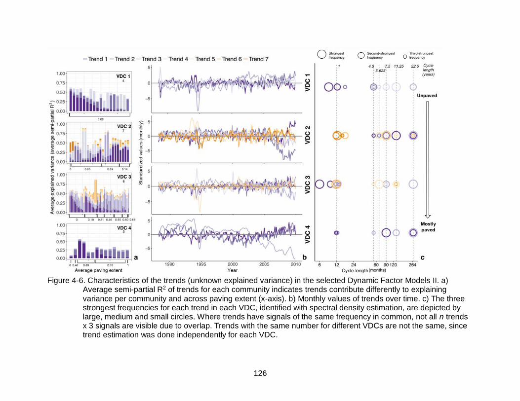
126
Figure 4-6. Characteristics of the trends (unknown explained variance) in the selected Dynamic Factor Models II. a)
Average semi-partial R2 of trends for each community indicates trends contribute differently to explaining variance per community and across paving extent (x-axis). b) Monthly values of trends over time. c) The three strongest frequencies for each trend in each VDC, identified with spectral density estimation, are depicted by large, medium and small circles. Where trends have signals of the same frequency in common, not all n trends x 3 signals are visible due to overlap. Trends with the same number for different VDCs are not the same, since trend estimation was done independently for each VDC.

127
Figure 4-7. Flow chart of methods

128
CHAPTER 5 CAUSALITY ANALYSIS OF REGIONAL BIOPHYSICAL AND VEGETATION VARIABLES REVEALS INCREASED FEEDBACK ALONG A ROAD PAVING
GRADIENT IN THE SW AMAZON
Background
Infrastructure development is an essential component of economic development
for many countries, but socio-economic benefits are often accompanied by negative
impacts. Rural-urban migration, conflicts over natural resources, land degradation,
changes in natural disturbance regimes, impacts on abiotic processes, pollution and the
disruption of animal movement have been documented (Laurance et al., 2009; Nepstad
et al., 2001). For forest ecosystems, road construction and paving are the main drivers
of deforestation (Laurance et al., 2002a; Marsik et al., 2011). Besides such land cover
conversion from forest to non-forest, studies have also highlighted potential impacts on
vegetation dynamics. Vegetation dynamics in the simplest interpretation refer to the
growth and senescence of vegetation over time, however on a broader level they
convey the influence of biotic and abiotic processes, climate, and natural and
anthropogenic disturbance regimes on vegetation structure and productivity.
On localized scales, indications have been found that vegetation dynamics can
indeed differ after anthropogenic disturbances, while forest cover did not change. In a
Bolivian forest, regeneration after either natural or anthropogenic disturbances was
dissimilar, with differences in vegetation structure and phenology (Felton et al., 2006).
Specifically, there were less flowering and fruiting plants in anthropogenic gaps, and
more non-commercial pioneer species. Similarly, in Madagascar limited logging
disturbance had a permanent effect on forest structure (Brown and Gurevitch, 2004).
These changes in vegetation dynamics can have an effect on ecosystem goods and

129
services, ranging from local to global level, and from carbon storage to river flow
regulation (Foley et al., 2007). For instance, at local level, differences in tropical forest
structure limit certain wildlife populations in Panama (DeWalt et al., 2003), bat diversity
is affected by vegetation structure (Santos et al., 2016), and other research found that
productivity in the Amazon is mostly driven by canopy phenology, not radiation
(Restrepo-Coupe et al., 2013). Considering that vegetation dynamics play a role in
ecosystem services provision (Millennium Ecosystem Assessment, 2005), they are
particularly important in coupled natural and human (CNH) systems.
The Southwestern Amazon has been subject to highway paving since the 1980s.
The so-called MAP area, where the states of Madre de Dios (Peru), Acre (Brazil) and
Pando (Bolivia) meet is an area through which the Inter-Oceanic Highway (IOH) has
been built in recent years. This highway, connecting the Atlantic coast in Brazil and the
Pacific coast in Peru, was finalized in 2011. The area has been recognized as a
“biodiversity hotspot” (Killeen and Solorzano, 2008; Myers et al., 2000; Perz et al.,
2011a) and livelihoods have been and still are closely linked to natural resources
(Almeyda Zambrano et al., 2010; Perz et al., 2013c): the area is a typical example of a
CNH system. As expected, deforestation in the area is associated with roads and urban
centers (Southworth et al., 2011), though it is not clear how much deforestation
accelerates with increased access (Marsik et al., 2011). Previous field research in the
area concluded that deforestation and degradation can experience different impacts,
with forest plots experiencing slightly more effect on forest value by the proximity to the
IOH, than to urban centers (Baraloto et al., 2015). Overall, we do not have a long-term
view of what the system-wide effects of road construction in the area are on vegetation

130
dynamics, and if and how these have evolved over time. Differences in vegetation
dynamics would imply changes in structure and composition of vegetation, which in turn
means altered ecosystem services and a potential for impacts on livelihoods and the
environment.
Changes in vegetation dynamics are hard to evaluate at a regional scale
because they involve structural changes in vegetation that are time consuming and
costly to capture through local field studies, especially over time. Further, drawing
conclusions at a larger scale from field plots has been shown to be challenging (Fisher
et al., 2008). Hence, most ‘road ecology’ studies focus on effects near roads but do not
assess regional vegetation dynamics. In addition to this spatial scale, the temporal
component is important since road construction is an incremental process itself, and
impacts from the presence of roads can increase or decrease over time, they are rarely
once-off events, and they can lag behind actual road construction (Findlay and
Bourdages, 2000; Laurance et al., 2009). Considering the importance of vegetation
dynamics in the MAP area and probable impacts of highway paving, there is a need for
a spatio-temporal analysis of long-term vegetation dynamics to determine whether or
not there has been an alteration in vegetation dynamics, and if so, whether the drivers
of these dynamics have changed. The latter would imply there has been a shift in
system state and a change in connectivity.
In this study, we hypothesized that the causal network of long-term vegetation
dynamics and biophysical variables (and climate indices) differs across a gradient of
road paving extent. We expected that, for the time period we studied, undisturbed
forests are more resilient and show strong relationships with all variables since

131
climate/vegetation feedbacks have been reported in previous studies (Betts et al., 2004;
Notaro et al., 2006; Quesada et al., 2012). We anticipated that causal relationships
between biophysical variables and vegetation dynamics would change with more
paving, with more emphasis on precipitation and soil moisture, and less on temperature
influences. This stems from previous work that found that under fragmented or logged
conditions, forest becomes more sensitive to drought and moisture-related variables
(Laurance and Williamson, 2001; Nepstad et al., 2001).
In order to evaluate changes to vegetation dynamics over longer periods and
larger areas, we can use remotely sensed vegetation indices (such as the Normalized
Difference Vegetation Index, NDVI, or the Enhanced Vegetation Index, EVI) as a proxy
for vegetation dynamics (Asner et al., 2000; Bradley and Fleishman, 2008; Cabello et
al., 2012; Chambers et al., 2007; Huete et al., 2002; Reed et al., 1994; F. B. Silva et al.,
2013; Volante et al., 2012). We tested our hypothesis by analyzing remotely sensed
regional vegetation indices for clusters of communities along the IOH, and mapping
potential causality between vegetation dynamics and other biophysical variables, using
a combination of novel and traditional approaches. We did this at a relatively high
temporal resolution of one month, with the objective of specifically capturing changes in
vegetation dynamics within years, an indication of phenology and productivity
(Chambers et al., 2007; F. B. Silva et al., 2013).
The methods applied to construct causality networks are a combination of
relatively new and innovative approaches, Singular Spectrum Analysis (SSA) and
Convergent Cross Mapping (CCM). While there is no conclusive method to prove ‘real’
causality with mathematical methods from the perspective of science philosophy, these

132
techniques come closest to causality as it has been defined and employed by Wiener
and Granger (Granger, 1980; 1969; 1963); analyses based on (statistically significant)
predictability. The remainder of this paper uses the term causality in the same vein.
The traditional approach has been Granger Causality (GC) analysis, which relies
on the comparison of vector autoregressive models to establish whether or not a
variable is significant in improving predictions of another variable. The method has been
used in various fields with or without modifications (Guo et al., 2010; 2008), such as
neuroscience (Bressler and Seth, 2011), cognitive processing (Zhou et al., 2009),
development studies (Weinhold and Reis, 2001), and ecological and environmental
studies. (Damos, 2016; Detto et al., 2012; B. Jiang et al., 2015; Kaufmann et al., 2004;
2003; Tuttle and Salvucci, 2016). However, GC relies on the system dynamics being
separable and linear, and complex natural systems are generally assumed to contain
nonlinear deterministic components (Sugihara et al., 2012). Determinism means that the
system is not stochastic, and that that there are theoretically identifiable (fixed)
relationships between variables or components in a system. In cases such as these,
signals are not separable linearly since each will contain information associated with
another. Current methods such as SSA are based on Taken’s Theorem of time-delayed
embedding and state space reconstruction and can identify nonlinear signals reliably
(this will be explained later in this Chapter). In noisy time series, which are common in
environmental sciences, this is an important step. Finding signals and removing noise is
essential for the causality analyses. The systems within which these signals occur, can
be weakly or strongly coupled. This coupling strength refers to synchronization of
signals: strongly coupled systems have signals (i.e. dynamics) that are more

133
synchronized. This makes it harder to identify the direction of causality in these
systems. CCM analysis identifies causality and driving variables in low-dimensional
weakly coupled systems using these signals (BozorgMagham et al., 2015; Mønster et
al., 2016), and for systems where there are stronger coupled dynamics, extended CCM
can distinguish between true bidirectionality or strong unidirectional forcing (Ye et al.,
2015). ‘Low-dimensionality’ implies there is a limited number of variables (‘dimensions’)
involved in explaining the system, generally less than 6. This is another reason why the
identification of signals is important before causality testing: some high-dimensional
(more complex) systems can still be partly explained with low-dimensional
representations of it.
We follow the approach by Huffaker et al. (2016b; 2017) to separate signals from
the original time series, and extensively test signals for stationarity, determinism and
eventually causal relationships. Stationarity and determinism are important for the
causality analysis as it requires a certain degree of stability in the signals to obtain
reliable results. Since these conditions have to met before it is justified to test for
causality with CCM, it is possible that variables ‘fail’ these tests. This indicates that they
are potentially high-dimensional or linear stochastic, and we need to turn to other
methods (Figure 5-1). We can apply GC analysis in these cases, and we can use
Multivariate SSA (MSSA) first to remove shared seasonality across time series.
Removal of shared seasonality, as advocated but also cautioned for by Granger (1979),
is generally done to avoid that synchronized seasonality overpowers the GC analysis. It
has been in done in several ways in the past (Papagiannopoulou et al., 2017; Tuttle and
Salvucci, 2016), usually involving some form of model building to simulate seasonality.

134
MSSA is an extension of SSA and is ideally suited for removal of seasonality, since it
does not require (subjective) models and can identify a number of frequencies across
various time series. Explanation and results of tests with GC causality are not discussed
in this Chapter, but can be found in Appendix C.
We apply SSA and CCM to a data set for the MAP area for a 23-year period
(1987-2009), for communities along the IOH that experienced highway construction at
different points in time. For 99 communities we obtained a long-term Enhanced
Vegetation Index (EVI2), maximum temperature, minimum temperature, potential
evapotranspiration, precipitation, soil moisture, all from re-analysis data sets. These
variables have been highlighted in numerous Amazon-wide studies as potential driving
factors (Betts et al., 2004; Gloor et al., 2015; Phillips et al., 2009; Quesada et al., 2012),
and are available at sufficient resolution. We also included the Multivariate ENSO Index
(MEI), Atlantic Multidecadal Oscillation (AMO) and the Pacific Decadal Oscillation
(PDO) since previous research found them strongly correlated with global,
hemispherical and continental carbon fluxes and climatic variables (Z. Zhu et al., 2017).
We applied time series-based cluster analysis to cluster the communities according to
similar vegetation dynamics and associated these with road paving extent. All analyses
were implemented per cluster, on area-weighted average time series, and results were
compared.
The objective of this Chapter is multi-faceted: first, to determine whether there
are differences in vegetation dynamics between areas, and characterize them. This will
be done with clustering and signal extraction. Second, to identify and compare driving
forces in each area which will be achieved by mapping causal networks. Finally, all of
135
these components combined give us a comprehensive overview of vegetation dynamics
along a road paving gradient and enable us to identify differences and similarities.
Materials and Methods
Study Site and Data
Study site
The 99 communities included in this study lie within the states of Madre de Dios
(Peru), Acre (Brazil) and Pando (Bolivia), also referred to as the “MAP” region. The area
lies between 9°48’ S and 13°1’ S latitude and 67°10’ and 70°31’ W longitude, at the foot
of the Andes Mountains and in the headwaters of tributaries of the Amazon River. The
climate is tropical, classified as Awi (Köppen climate classification), with an average
daily temperature of 25° C and mean annual precipitation of approximately 2000 mm.
The dry season runs from June to October, in which monthly rainfall averages < 100
mm. The types of forest in the area are dense tropical forest, open tropical forest with
palm trees, and open forests dominated by bamboo – with many locations containing a
mix of these forest types (Carvalho et al., 2013; Rockwell et al., 2014; Salimon et al.,
2011). The Inter-Oceanic Highway was paved between approximately 1992 (Rio
Branco) and 2011 (Peru). Communities in Bolivia still had unpaved roads during the
time period studied since road paving had not progressed much further than Cobija.
These are resource-dependent rural communities that were part of earlier studies (Perz
et al., 2013b; 2013a; 2011b). They are defined in these as being “distinct land tenure
units and/or population centers”. This ensures that any effects on vegetation within a
community results from the same land tenure arrangements and management
decisions.

136
Highway paving
Highway paving histories were provided from previous studies (Perz et al.,
2013b). It is a value between 0 and 1 representing proportion of a road segment paved,
and is derived from field work. The year when paving of the road segment along which a
community sits is finalized is taken as the starting point to estimate increments in the
proportion paved. If a community is along a highway segment between two towns that
was paved by 1999, that community gets a value of “1” for 1999 (and subsequent
years). Proportions paved in the years prior are derived from field notes with the timing
of the onset and conclusion of paving of that segment, with a linear interpolation of
paving proportions during the intervening time period.
Vegetation dynamics: EVI2
Data for the enhanced vegetation index (EVI2) used in this analysis were
obtained from the University of Arizona’s Vegetation Index and Phenology (VIP) lab,
which applies an algorithm to translate two-band data from the Advanced Very High
Resolution Radiometer (AVHRR) into MODIS EVI (Z. Jiang et al., 2008). AVHRR data
have been collected since 1982. The data used in this analysis (1987-2009) were
obtained from the VIP lab in October 2013 in monthly time steps and at a 0.05°
resolution. Area-weighted time series were extracted for each community polygon. Data
correction was performed to address outliers and discrepancies between AVHRR-
derived EVI (1982-1999) and MODIS EVI (2000-2010), because AVHRR-derived EVI
exhibited consistently lower values (an overall average of 0.387 vs. 0.513), see the link
in Supplementary Materials to data and code. This is attributed to the lower quality of
AVHRR data in areas with high cloud density (pers. comm. Dr. K. Didan). For the
remainder of this study, this variable will be referred to as EVI or vegetation dynamics.

137
Biophysical variables from reanalysis data sets
Monthly data sets were sourced in June 2013 from the Climatic Research Unit
(CRU) at the University of East Anglia. Covariates include the minimum, mean and
maximum temperatures, precipitation and potential evapotranspiration (MINT, MEANT,
MAXT, P, PET). The mean, minimum and maximum temperatures (in °C) and
precipitation (in mm) were obtained at a resolution of 0.5 x 0.5° (Harris et al., 2013), and
were assigned to each community polygon in an area-weighted manner. Potential
evapotranspiration (in mm) is also included in the CRU data set, and is calculated from
a variant of the Penman-Monteith formula, using mean, minimum and maximum
temperature, vapor pressure and cloud cover (Harris et al., 2013).
Soil moisture (SM) comes from the NOAA Climate Prediction Center (CPC)
model at a resolution of 0.5 x 0.5°, which uses CPC precipitation data and temperature
data from the NCEP/NCAR Reanalysis (Fan, 2004). The data are provided as average
soil moisture in terms of water height equivalents (mm). As with the other data sets, the
soil moisture data are calculated as an area-weighted time series for each community
polygon.
Climate indices
The AMO, PDO and MEI time series were all obtained from the NOAA Earth
System Research Laboratory. For the AMO we used the unsmoothed version (Enfield et
al., 2001). This time series is an index of surface temperature of the North Atlantic
Ocean. The PDO consists of the first principal component of monthly anomalies of sea
surface temperature of the North Pacific Ocean (Mantua et al., 1997; Zhang et al.,
1997). The MEI is a composite index that is believed to better reflect the El
Niño/Southern Oscillation (ENSO) phenomenon than simply sea surface temperatures

138
(Wolter and Timlin, 2012). It incorporates sea level pressure, surface air temperature,
sea surface temperature, cloudiness fraction, zonal and meridional components of
surface wind over the tropical Pacific Ocean.
All data used in analyses described below were normalized first.
Methods
Time series clustering
We applied a time series clustering based on an adaptive similarity matrix
(Chouakria and Nagabhushan, 2007). In order to cluster variables based on their
shared dynamics and not just values, this method contains a scaling function which
allows both behavior as well as values to be taken into account the similarity matrix
calculation. Behavior is defined as the direction and steepness of the time series
between two points in time. Parameter 𝑘, which ranges from 0 to 5 determines how
much behavior contributes to the similarity matrix, see Equations 3-1 through 3-4 in
Chapter 3. Behavior similarity is expressed as temporal correlation, and Euclidian
distance is used for value similarity.
We used hierarchical clustering with Ward’s method for 1 to 10 clusters, and with
𝑘 varying between 0 and 5. To obtain the most objective selection of the appropriate
number of clusters, all results were evaluated with the Dunn Index and the Silhouette
Width (Brock et al., 2008), schemes that base validation only on the data themselves.
The Dunn Index compares within cluster variation (compactness) and the distance with
other clusters (separation). It compares the minimum distance between points not in the
same cluster and the maximum within-cluster distance, and ranges from 0 to infinity.
The Silhouette Width attempts the same, but by comparing each point to its own cluster
(cohesion) and to other clusters (separation), with the final value being the average over

139
all points in the cluster. It lies between -1 and 1, and should be above 0 for decently
separated clusters. Negative values indicate some clusters overlap. Both measures
should be maximized. We chose the number of clusters that maximized both indicators.
After clustering, all variables (except climate indices) were transformed to area-
weighted averages for each VDC for further analysis.
Singular spectrum analysis
Phase space, the plotting of time series against its own lagged versions, is the
basis for analysis of dynamic systems with deterministic components, which is known
as Taken’s Theorem. In a system with causal variables, plotting these against each
other in phase space (e.g. in 3D for 3 variables) will reveal an attractor, a specific
pattern or path. Examples are predator-prey relationships or the Lorenz attractor. Often
though, we do not know the causal relationships from which to construct an attractor.
Taken’s Theorem states that if we apply an appropriate lag to a time series, and plot
these lagged versions, we can obtain a shadow attractor which is topologically similar to
the real attractor. These properties can be used in causality analysis.
Real-life time series are often subject to a fair amount of noise, particularly in
ecology and environmental sciences. The first step is to separate noise and signals in
the time series, since noise complicates the construction of an attractor (Figure 5-1).
SSA deconstructs and reconstructs time series by identifying regular oscillatory
components of different frequencies (deconstruction) which are simply added together
to reconstruct the ‘signal’ of the time series. It is based on decomposition of time series
into orthogonal components through Singular Value Decomposition (SVD) of a Toeplitz
matrix (Golyandina, 2010). A Toeplitz matrix contains lagged copies of the original time

140
series in its columns, which makes it a matrix with constant diagonals from left to right.
For a matrix 𝐿 × 𝐾 this takes the form:
𝑇 = (
𝑡𝐾 𝑡𝐾−1
𝑡𝐾+1 𝑡𝐾
⋮ ⋮𝑡𝐾+𝐿−1 𝑡𝐾+𝐿−2
⋯ 𝑡2
⋯ 𝑡3
⋯ ⋮ ⋯ 𝑡𝐿+1
𝑡1
𝑡2
⋮𝑡𝐾
)
The window length (the number of columns) for creating the matrix was the multiple of
the dominant periodic component of the data, not exceeding N/2 (N = number of
observations in the time series). Using this window length makes it more likely that SSA
will find the most important frequencies (or periodic components) in the time series. The
dominant periodic component was determined by spectral analysis, which applies a
Fourier transform and returns the power spectral density of frequencies present in the
time series.
The SVD aims to separate the original Toeplitz matrix into elementary matrices.
The method returns so-called eigentriples: each is a combination of a singular value
(the square root of an eigenvalue), a left eigenvector and a right eigenvector.
Multiplication of the singular value, left eigenvector and transposed right eigenvector
gives an elementary matrix (Golyandina and Zhigljavsky, 2013). The original Toeplitz
matrix is the sum of all elementary matrices. Some of the eigentriples (or elementary
matrices) can be grouped together to form unique, separable signals – which is what we
are after for signal reconstruction. To decide which to group together, first the
elementary matrices are converted to time series with diagonal averaging: averages of
diagonals give the time series values at each time 𝑡 (see for instance the layout of
theToeplitz matrix, diagonal averaging will return the original time series). This produces
a large number of time series, which when added together form the original time series.

141
However, we are not interested in all these components. Decomposing the original time
series in periodic components and noise (and sometimes a trend), the purpose of SSA,
is only informative if these additive components are separable. This can be evaluated
with a w-correlation matrix, the weighted correlation between the time series
components obtained through the SVD and diagonal averaging. The weight reflects the
number of times an element appears in the elementary matrix (explained in detail in
Golyandina et al. (2013)). This correlation is a measure of orthogonality (0) or non-
orthogonality (1) of two time series. We can also perform visual inspection of
scatterplots of pairs. Paired periodic time series with the same frequencies will exhibit
high correlation with each other and not with others, and will form regular shapes when
plotted against each other in a scatterplot. The selected time series components (i.e.
eigentriple pairs) are the basis of oscillatory components of the time series and after
extraction, and then addition form the ‘reconstructed’ time series. The contribution to the
decomposition by each periodic time series was calculated as the weighted norm of the
eigenvectors as percentage of the total weighted norm of the original time series.
Adding those of the selected periodic time series signify the total contribution to the
decomposition by the ‘reconstructed’ time series - which we can term the ‘signal’. All the
steps incorporated in this method ensure that the signal is separable from the noise.
To test for stationarity of the signals, nonlinear cross-prediction was employed
(Huffaker et al., 2017). This method measures the skill with which segments of the time
series predict other segments of the same time series using nonlinear prediction
methods. If the prediction skill decreases with remote segments, the time series is
deemed non-stationary. The method starts with dividing the series into segments, and

142
for each the appropriate embedding dimension is calculated (i.e. the maximum lag at
which lagged time series of the original still share information with the original – the first
average mutual information index minimum for the series). These segments are then
embedded with this lag to create matrices with lagged copies of themselves. Each is
used as learning and testing sets alternatively: as a testing set the segment is used to
predict future points using the nearest neighbors approach. These predictions are then
evaluated against a learning set using the Nash-Sutcliffe coefficient, a measure of
goodness-of-fit (Huffaker et al., 2016b; Nash and Sutcliffe, 1970; Ritter and Muñoz-
Carpena, 2013b); i.e. if we have 5 segments, each will be used to predict the other 4.
After confirming stationarity, surrogate data testing was applied to provide
statistical proof of the likelihood that the reconstructed time series is not generated by a
linear stochastic system, but by a deterministic system. This done by shifting values in
the time series in such a way that the serial structure is destroyed, but the statistical
properties are conserved. The surrogate data that are produced is then tested for
characteristics of nonlinear dynamics, comparing those to the characteristics of the
original signal. The null hypothesis is that the signal is generated by a linear stochastic
system – meaning that the characteristics of the surrogate data resemble those of the
signal. This type of testing is widely accepted as a suitable measure to test the null
hypothesis of a time series being a representation of a particular type of system (Dolan
and Spano, 2001; Small and Tse, 2003; 2002; Theiler et al., 1992). The surrogate data
testing approach we applied for this study has been used in previous studies (Huffaker,
2015; Huffaker et al., 2017; 2016b), and guidance on implementation has been taken
from these works. We also refer to these documents for the detailed methodology and

143
implementation. We applied algorithms that produce amplitude-adjusted Fourier
transform (AAFT) surrogates (Theiler et al., 1992) and pseudoperiodic (PPS) surrogates
(Small and Tse, 2003). The double surrogate testing covers two potential types of data:
linearly filtered noise processes (AAFT) and periodic orbits with uncorrelated noise
(PPS). The discriminating statistics that were estimated were nonlinear prediction skill
and entropy complexity. The prediction skill is expressed as the Nash-Sutcliffe
coefficient of efficiency, NSE (Ritter and Muñoz-Carpena, 2013a), which is calculated
for the earlier described nonlinear prediction of segments of the time series of other
segments of itself (Sugihara et al., 2012). Entropy complexity expresses uncertainty and
randomness of a data set: lower values point to high predictability whereas higher
values indicate independently and uniformly distributed values (the null hypothesis). For
the tests, nonparametric rank order statistics were applied, with 𝛼=0.05 and parameter
𝑘=5 (the number of surrogates needed for values of 𝛼) to give us 𝑆 = (𝑘 𝛼⁄ ) − 1 = 99
surrogates for a one-tailed hypothesis test. The null hypothesis is accepted if the
statistic value of the signal falls within the 𝑘 largest or smallest values produced by the
surrogates. The test for prediction skill is an upper-tailed test since we only reject the
null hypothesis if the surrogate data predict with better skill than the signal. The test for
entropy complexity is a lower-tailed test as we are looking for lower entropy values for
the signal than the surrogate data. If the null hypothesis is rejected, we conclude there
is sufficient evidence for deterministic structure and use the signals for further causality
analysis.

144
Convergent cross mapping
CCM is a relatively new method (Sugihara et al., 2012), but has gained a lot of
popularity over the years with a number of variations in implemented on different types
of data sets (Clark et al., 2015; Huffaker et al., 2016a; Ma et al., 2014; Mønster et al.,
2016; Van Nes et al., 2015). We used the original approach by (Sugihara et al., 2012)
as implemented by (Huffaker et al., 2017). This method is based on phase space
reconstructions: if two variables interact in a deterministic fashion with each other,
phase space reconstruction of each variable with delayed coordinates (shadow
attractors) would map exactly onto the phase space that we could create from both
variables (the original attractor). Hence they should also map perfectly to each other.
CCM takes a shadow attractor for 𝑋, and with a nonlinear prediction algorithm (nearest
neighbors) estimates points on another shadow attractor 𝑌. The Pearson’s correlation
coefficient (𝜌) between the original and estimated points of the second shadow attractor
𝑌 is referred to as cross-map skill, see Sugihara et al. (2012) and Huffaker et al. (2017)
for details. If this is high, 𝑋 has causal influence on 𝑌. There is a convergence
requirement: that the cross-map skill should converge to a certain value as the time
series portion used for cross-mapping (libraries) gets longer. The final value for 𝜌 is the
average of a fraction of the total libraries tested. We set this fraction to 0.33, of the last
(longest) libraries tested. Only 𝜌 ≥ 0.65 were included in causal network construction.
CCM has been found to work well on systems with weak to moderate coupling.
However, in systems with strong unidirectional forcing, ‘generalized synchronicity’ can
occur, with high cross-mapping skill both ways (Sugihara et al., 2012). Regular CCM
generally cannot distinguish between true bidirectional causality, or strong unidirectional

145
forcing. By forcing asynchrony on the data though, the true directionality can be
established (Ye et al., 2015). Extended CCM applies both positive and negative lags to
the driving signal. If it is truly the driving signal, the highest 𝜌 will be detected at a
negative lag as the dynamic of the driver has to occur first. Variables with 𝜌 ≥ 0.65 but
their highest 𝜌 at a positive lag were deemed false positives and not drivers. Only
results where the difference between the 𝜌𝑚𝑖𝑛 and 𝜌𝑚𝑎𝑥 was larger than 0.05 ∙ 𝜌𝑚𝑖𝑛
were considered (Huffaker et al., 2017). The lags have additional significance, in the
sense that they can indicate the order of effects in a transitive network (Ye et al., 2015).
Data Availability
Data collected and processed for this study can be found at
10.6084/m9.figshare.c.3933388, as well as the R code that was used for processing
and analysis.
Results
Identification of Four Vegetation Dynamics Clusters along a Road Paving Gradient
The time series clustering resulted in the identification of 4 clusters, with behavior
contributing 76.2% to the similarity matrix (𝑘 = 2). These clusters also showed spatial
consistency (Figure 5-2a). In the remainder of this study they will be referred to as
Vegetation Dynamics Clusters (VDCs). The collection of EVI time series per VDC
shows different temporal patterns (Figure 5-2b), though their long-term average, median
and standard deviations are similar for each VDC.
The area-weighted average road paving was calculated for each VDC (Figure 5-
2d), and the average road paving for each community individually (Figure 5-2c) was
plotted per VDC in a boxplot (Figure 5-2e). Based on the distinct differences in the time

146
series in Figure 5-2b, and the exponential trend in paving extent (a loess curve through
the medians), VDCs were ordered from least associated with road paving to highly
associated with road paving. VDCs 1 and 4 and be considered the two extreme states,
unpaved and paved, within the system. VDC 2 and 3 are then transitional in terms of
road paving, with most communities having had road paving less than 50% of the study
period.
Signal separation reveals different signals for vegetation in each VDC
The analysis reconstructed different EVI signals for each VDC, with different
periodicities (see Figure 5-3, Table 5-1, Figures B-2 to B-6). All signals have a 12-month
oscillation, but the presence of oscillations of 4, 5 or 6 months vary between VDCs.
There is also a difference in the periodicity of the low-frequency signals. Figure 5-4
demonstrates the differences between the VDCs even clearer, and also shows there is
general agreement of patterns of low and high EVI values between observed data (first
column) and reconstructed data (second column). For VDC 1, lower EVI values occur
from June to August, but there is another dry period in some years at the beginning of
the year. This is less prominent in the other VDCs. Higher EVI values are stronger in
October-December for VDC 1 and 2, less strong for VDC 3 and 4. The low frequency
signals are visible as bands of years with lower EVI around 1992-1995 and 2000-2004
for VDC 2 for example, but with more frequent low EVI years for VDC 4.
We found that even though the reconstructed signals for biophysical variables
seemed similar between VDCs (Figure 5-3), the periodicities used for reconstruction
were different (Table 5-1). Cycles of 12 and 6 months persisted for all VDCs for
maximum, mean and minimum temperature as well as PET, and precipitation and soil
moisture also had a clear annual cycle. Beyond that, there is a large variation in cycles

147
included in the signals. It is of interest to note that for all biophysical variables the lower
frequency periodicities mostly occur in VDC 3 and/or 4. Variables with the most
variation between VDCs are maximum temperature and precipitation, which is clear in
B-7. Precipitation in VDC 4 has a more distinct low frequency signal, with drier and
wetter periods of about 4 years. Across all VDCs, higher maximum temperatures
appear to slowly shift to occur slightly earlier in the year. The soil moisture signal lags
about 2 months behind precipitation: June-September is a drier period, but soil moisture
drops below average in August-November. The contribution to the decomposition is
high for most variables (Table 5-1), with EVI and maximum temperature yielding the
lower contributions (40-60%).
For the climate indices, MEI shows periodicities of approximately 5 years, 2-3
years and 9 months, which is in line with previous studies (Kuss and Gurdak, 2014;
Park and Dusek, 2013; Roy, 2010; Velasco et al., 2017). The AMO contains
periodicities of 8.3 years, approximately 1 year, and 4.5 months. The PDO contains an
annual periodicity, 2.5 years and almost 2 years. Due to the length of the time series,
we are potentially missing out on longer temporal cycles, since other studies also found
15-25 year cycles for the PDO and 50-70 year cycles for the AMO (D'Aleo and
Easterbrook, 2010; Kuss and Gurdak, 2014; Park and Dusek, 2013). This probably also
explains the lower contribution to decomposition for the PDO (40%) and AMO (46%).
The nonlinear predictive skill for the variables was tested using 5 segments
(Figure B-8). We concluded that for VDC 4 the EVI is non-stationary, with a clear
downward skill, making it unsuitable for further CCM analysis. For the other VDCs and
the climate variables, while the skill was low for some variables and somewhat

148
ambiguous in some cases (e.g. AMO), we decided there is sufficient stationarity to
continue with subsequent testing for determinism. Surrogate data testing rejected the
null hypothesis of linear stochastic dynamics with either surrogate test, AAFT or PPS,
for all signals based on both discriminating statistics (predictive skill and entropy
complexity). For two signals, EVI signals for VDC 2, and mean temperature for VDC 3,
the rejection is not as strong as for others (Table 5-2).
Causality testing of signals for three VDCs indicates an increase in causal relationships for EVI
As outlined in the methods, after calculating the cross-mapping skill 𝜌 (Table B-
2), we applied extended CCM to distinguish bidirectionality from strong unidirectional
forcing for VDCs 1, 2 and 3 and climate variables. While our calculations generate
numeric results for passing or not passing extended CCM (see Methods), this
evaluation was also based on visual inspection of plots of the delays, as not all results
were as obvious as previous studies suggest they could be (Ye et al., 2015), see Table
B-3. The final results, for 𝜌 ≥ 0.65 and filtered with extended CCM are summarized in
Table 5-3. Note that the absence of 𝜌 does not imply there is no cross-mapping skill at
all; simply that it fell below the cut-off. Considering the dense network of causality that
appeared for this system, we wanted to focus on the most significant causal
connections.
Biophysical variables
This study shows biophysical variables in the Southwestern Amazon form a tight
causal network of their nonlinear deterministic components, with bidirectionality in all
ways for VDC 1 -3 (Table 5-3): maximum, average, minimum temperature, precipitation,
potential evapotranspiration and soil moisture. This points to strong feedback loops; and

149
these are not altered with the extent of highway paving. Extended CCM gives an
indication of order, since lags from this analysis differ per VDC (Table B-3). In the
following construction and discussion of causality networks the bidirectional
relationships for the biophysical variables are not depicted, to enhance the readability of
the graphs.
Climate variables
Figure 5-5 shows the CCM results for the nonlinear deterministic components for
EVI driving other variables. The results for variables driving EVI and climate indices,
and climate indices as drivers, are shown in Figure B-9. The AMO and MEI are being
driven by an increasing number of variables across the VDC 1-3. The MEI is mostly
driven by moisture-related variables; precipitation and soil moisture. While neither of
these could physically directly affect the MEI, we suspect there is an indirect effect here
through cloudiness and/or actual evapotranspiration. The AMO is more driven by
temperature-related variables; maximum and minimum temperature and potential
evapotranspiration. Again, we suspect that there is some relationship with cloudiness
and/or actual evapotranspiration. This would be a mechanistic explanation for the
influence of biophysical (local) variables on climate indices (Arias et al., 2010; Klein et
al., 1999). The AMO is the only climate index that appears to drive biophysical
variables, temperature and soil moisture. It is also the only climate index driving the
other two, the PDO and the MEI. Note that these results do not imply there was no
causal effect at all from the MEI onto the PDO or AMO, but its 𝜌 was below the cut-off
(Table B-2).
The indication that EVI drives the AMO across all three VDCs, and the MEI in
VDC 1 (Figure 5-5 and B-9), can be interpreted as indirect effects as well. The strength

150
of this causal relationship increases from VDC 1-3 (shown in the colors of the arrows in
Figure 5-5), but the number of causal relationships from EVI to biophysical variables
(Figure 5-5), as well as the number and strength of biophysical variables to the AMO
(Figure B-9) also increases along the VDCs. It is plausible that the mechanistic causal
path is from EVI to biophysical and/or atmospheric variables to (other, not included
variables to) sea surface temperature anomalies or climate indices.
Vegetation dynamics
The vegetation dynamics (EVI) signals are driven by all biophysical variables,
which does not change across VDCs – except for some variations in strength of the
causal relationships (Figure B-9). In VDC 1, maximum temperature, potential
evapotranspiration and soil moisture are the strongest drivers of EVI, while for VDC 3
this has evened out more, with only minimum temperature having a slightly stronger
influence. Surprisingly, we see an increase in feedback from EVI from VDC 1 to 3
(Figure 5-5): whereas EVI does not seem to drive any of the biophysical variables in
VDC 1, this increases to EVI driving maximum, mean and minimum temperature,
precipitation and soil moisture in VDC 3.
Discussion
Vegetation Dynamics Clusters and Signals
From the cluster analysis results, we conclude there are indeed clusters of
vegetation dynamics that are distinguishable based on their values and, mostly, their
temporal behavior. The signals extracted from the area-weighted time series provide
more support for this as EVI signals incorporate different frequencies. This is an
interesting finding considering that previous research considered the whole area to be in
one particular ‘phenoregion’ (F. B. Silva et al., 2013). That study divided the Amazon in

151
regions based on intra-annual variation in NDVI, and the MAP area fell into a region
with “evergreen forest in high lands” with a dry season from June to August, with
potentially a small area of our study area in Peru, falling in “bamboo forest” with a dry
season from May to September. NDVI and EVI are not the same though, and EVI is
known for better reflecting vegetation changes in dense forest and tropical regions
(Huete et al., 2002). This study highlights that the forests in the Amazon are even more
heterogeneous than suggested in previous studies – though we offer support for the
hypothesis that in our study area this is due to anthropogenic influences, specifically
highway paving. Another potential explanation for the VDCs or any changes that we see
across VDCs could be soil or forest types (Baraloto et al., 2015; Quesada et al., 2012).
However, a classification for this area (in development) indicates that on average
respectively 78%, 57%, 87% and 69% of VDCs 1-4 are “terra firme forest over soils with
low/medium fertility, with bamboo and without bamboo” and the remaining areas are
different types of flooded forest. In the absence of any other variables currently along
which to order VDCs, the road paving gradient is intuitive.
Application of Causality Analyses on Complex Systems: Implications of Findings and Methods
Scientific findings
The strong bidirectional biophysical network that we identified is a finding that is
to be expected for this area: vegetation in tropical areas, specifically the Amazon, are
known for their feedback loops (Betts et al., 2004; Quesada et al., 2012). It is
encouraging to see that these connections were maintained across 3 VDCs, which
indicates resilience in the system. It could be argued that ‘true’ bidirectionality is
physically not possible: two variables cannot change at the same time and also drive
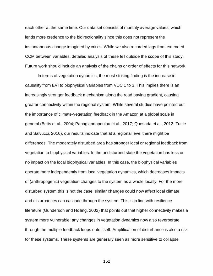
152
each other at the same time. Our data set consists of monthly average values, which
lends more credence to the bidirectionality since this does not represent the
instantaneous change imagined by critics. While we also recorded lags from extended
CCM between variables, detailed analysis of these fell outside the scope of this study.
Future work should include an analysis of the chains or order of effects for this network.
In terms of vegetation dynamics, the most striking finding is the increase in
causality from EVI to biophysical variables from VDC 1 to 3. This implies there is an
increasingly stronger feedback mechanism along the road paving gradient, causing
greater connectivity within the regional system. While several studies have pointed out
the importance of climate-vegetation feedback in the Amazon at a global scale in
general (Betts et al., 2004; Papagiannopoulou et al., 2017; Quesada et al., 2012; Tuttle
and Salvucci, 2016), our results indicate that at a regional level there might be
differences. The moderately disturbed area has stronger local or regional feedback from
vegetation to biophysical variables. In the undisturbed state the vegetation has less or
no impact on the local biophysical variables. In this case, the biophysical variables
operate more independently from local vegetation dynamics, which decreases impacts
of (anthropogenic) vegetation changes to the system as a whole locally. For the more
disturbed system this is not the case: similar changes could now affect local climate,
and disturbances can cascade through the system. This is in line with resilience
literature (Gunderson and Holling, 2002) that points out that higher connectivity makes a
system more vulnerable: any changes in vegetation dynamics now also reverberate
through the multiple feedback loops onto itself. Amplification of disturbance is also a risk
for these systems. These systems are generally seen as more sensitive to collapse

153
(Gunderson and Holling, 2002). Why there is an increase in connectivity cannot be
definitively answered with these results and requires further research. We pose that the
different vegetation dynamics (and thus different causal network) means the structure
and composition of vegetation differs between the unpaved and paved state, with the
paved state containing vegetation that interacts more with biophysical variables. Most
likely the vegetation is more strongly seasonal, hence mechanistic processes such as
stomatal opening and closing (affecting evapotranspiration and carbon exchange with
the atmosphere) and greening/senescence have a more direct effect on local
biophysical variables.
Stationarity results of the EVI excluded VDC 4 from CCM analysis, which is
another important finding of this study. This result implies that this system, specifically
vegetation dynamics, is already undergoing some change (at the regional level). This is
one of the more defined states, i.e. the paved state, so it would be important to
understand the dynamics in more detail. In particular since this is the state that all other
VDCs are trending towards in terms of paving status. It is suggested to do more
research on the EVI signal, potentially exploring signals and causality for segments of
the time series. Further work into change point analysis is also recommended, ideally at
the community level.
Even though the relationships between the AMO, PDO and MEI were not the
main objective of this study, we found that the relationships we identified for the
deterministic components of the time series confirm and clarify previous work (Enfield et
al., 2001; Kuss and Gurdak, 2014; Roy, 2010). The AMO appears to be the most
influential climate index in our study area. This study adds insight to the relationship

154
between climate indices and biophysical variables, but there is a need for further
research on the actual mechanisms linking these. The methods applied here go beyond
correlation analyses which often leave questions of drivers (Wang et al., 2013), but
reveal the directionality of causality clearer. We must caution that the length of the time
series could have prevented us from picking up longer term oscillations that might be
relevant as well, and that the results presented in Figure 5-5 and B-9 do not imply a
complete absence of causality between some indices, simply that they were below the
cut-off (see Table 5-3 and Table B-2). Also, we cannot assume we have included all
variables that could fill in the complete causal path. Variables such as actual
evapotranspiration, evaporation, cloudiness and wind could be important in sea surface
temperature anomalies, as previous studies have suggested that these play a role
(Klein et al., 1999; Mitchell and Wallace, 1992). Another study that examined sea level
pressure and sea surface temperature concluded that in the atmosphere-ocean
interaction, it is the atmosphere driving the ocean (Davis, 1976). This gives credence to
the findings in this study, though confirmation of causality of these global phenomena
would have to come from a much larger and comprehensive study incorporating several
regions.
Applicability of methods
While we propose that (nonlinear deterministic) CCM is more suitable than (linear
stochastic) GC analysis for a system as the one we studied here, there are caveats to
consider with this method too. The length of the time series influences the signals that
can be identified with SSA, especially low frequency signals. The quality of the
reconstructed signals is dependent on the interpretation of the researcher as well. Up to
now, there are not many guidelines on cut-offs for separability, stationarity or causal

155
strength. And as we found in this study, if a signal appears to undergo change over the
course of the time period (VDC 4), CCM cannot be applied. Finally, if a system has no
low-dimensional deterministic structure, but is instead high dimensional, CCM is not a
suitable causality detection method. In this study, as will be the case with many studies
of environmental systems, there still remains the question how much a reconstructed
signal should contribute to the decomposition to be deemed a ‘strong’ enough signal.
EVI scored the lowest in this regard, but because of the inherent noisiness of this data,
we deemed it sufficient to proceed with CCM.
Lastly, while extended CCM is very promising, application to strongly coupled
systems with bidirectionality gives ambiguous results in terms of values and shapes of
results over all the tested lags. We used a rather arbitrary cutoff of 0.05 ∙ 𝜌𝑚𝑖𝑛 to decide
whether or not to evaluate the results from the lagged CCM, but further research is
required on appropriate cutoffs, especially in the light of results that do not exhibit the
typical ‘hump’ in results (i.e. one clear 𝜌𝑚𝑎𝑥 across results from the lagged CCM).
Lastly, as has been expressed throughout this study, there is always the possibility that
variables that are of importance have not been included. Some of these are actual
evapotranspiration, cloudiness, fire, and potentially anthropogenic variables that vary
monthly or intra-annually (water use, food or timber prizes).
Concluding Remarks
This research has provided support to our hypothesis that vegetation dynamics
differ along a road paving gradient, not just in their appearance (the signal), but also
structurally. All biophysical indicators are implicated as drivers across the VDCs
associated with road paving, with varying strength. Most notably though, is an increase
in feedback from vegetation onto biophysical indicators, locally, with increased paving.

156
Also, the different nature of the vegetation dynamics signal in the paved state (VDC 4),
which excludes it as a candidate for CCM analysis, is of interest. Non-stationarity
implies a change in the signal over time. This suggests that increased infrastructure
development could lead to a more locally connected system, which would be more
sensitive to (anthropogenic) disturbances due to amplification. While this is not
necessarily a new suggestion, we have been able to back this up with real-life data.
Unfortunately, the exact mechanics behind this cannot be pinpointed with this research,
but should be the focus of further research.
The results of this study provide support for policies that aim at monitoring a suite
of variables after highway paving has been implemented. Studies have suggested that
imminent thresholds and regime shifts can be detected from time series by monitoring
critical slowing down, in terms of recovery of variance and autocorrelation after
disturbances (Dakos et al., 2014; 2011; 2012; Scheffer et al., 2009). With vegetation
dynamics being a difficult variable to monitor and measure at larger scales in tropical
areas, it is recommended to intensively measure other local variables such as the ones
included in this study: the most straightforward ones being temperature and
precipitation. Considering the increased connectivity with increased road paving, these
could be indicators of impending (local) system changes. With forest areas worldwide
under threat of the current infrastructure development paradigm (Laurance et al., 2014),
monitoring forest areas and limiting impacts should be high on the agenda of any nation
or development agency.

157
Table 5-1. Periodicities that were selected to create reconstructed signals of time series and the contribution of each signal to the decomposition (value of the weighted norm of the signal as percentage of the total weighted norm of the time series). Total contribution of the signals combined is highlighted in bold. EVI2 = Enhanced vegetation Index2, MAXT = maximum temperature, MEANT = average temperature, MINT = minimum temperature, P = precipitation, PET = potential evapotranspiration, SM = soil moisture, AMO = Atlantic Multidecadal Oscillation, PDO = Pacific Decadal Oscillation, MEI = Multivariate ENSO Index.
VDC 1 VDC 2 VDC 3 VDC 4
Periodicity (months)
Decomposition contribution
Periodicity (months)
Decomposition contribution
Periodicity (months)
Decomposition contribution
Periodicity (months)
Decomposition contribution
EVI2 31.1 12.0 6.1 4.0
47% 19% 20% 4% 4%
12.0 36.0 33.3 4.9 4.4
44% 19% 16% 5% 2% 2%
12.0 46.4 6.1 9.1
49% 26% 15% 5% 3%
12.0 40.6 19.8 4.7 3.7
41% 24% 14% 2% 1% 1%
MAXT 12.0 6.0 4.0
55% 33% 20% 2%
12.0 6.0 4.0 13.8
58% 32% 21% 3% 2%
12.0 6.0 30.8 10.9 4.1
60% 33% 17% 4% 3% 3%
12.0 6.0 6.4 4.0
57% 32% 21% 2% 2%
MEANT 12.0 6.0 2.2
63% 43% 19% 1%
12.0 6.0 3.3 6.4
66% 50% 14% 1% 1%
12.0 6.0 5.3 4.0 19.3 6.2
70% 46% 15% 3% 3% 2% 1%
12.0 6.0 6.3
131.0
65% 40% 20% 3% 2%

158
Table 5-1. Continued.
VDC 1 VDC 2 VDC 3 VDC 4
Periodicity (months)
Decomposition contribution
Periodicity (months)
Decomposition contribution
Periodicity (months)
Decomposition contribution
Periodicity (months)
Decomposition contribution
MINT 12.0 6.0 15.9 2.7 6.3 2.2
86% 70% 12% 1% 1% 1% 1%
12.0 6.0 2.7 2.8
82% 73% 7% 1% 1%
12.0 6.0 4.0
84% 73% 9% 2%
12.0 6.0 5.3 4.0 12.1 6.3 6.3 2.7 2.8
89% 70% 13% 1% 1% 1% 1% 1% 1%
0.4%
P 12.0 13.7 10.3
64% 60% 3% 1%
12.0 6.0 4.0 2.2
6.1
69% 59% 4% 3% 2% 1%
12.0 20.3 4.0 2.2 4.0 5.6 5.6
67% 59% 3% 3% 2% 2% 2% 1%
12.0 47.1 12.8
63% 48% 9% 6%
PET 12.0 6.0 4.0 2.4 3.0 12.0
89% 75% 10% 2% 1% 1%
0.3%
12.0 6.0 4.0 6.0 2.4 6.5
90% 71% 11% 5% 1% 1% 1%
12.0 6.0 4.0 3.0 2.4 9.0
89% 74% 9% 4% 1% 1%
0.3%
12.0 6.0 3.9 3.0 2.4 27.8 13.7
90% 72% 11% 2% 2% 2%
0.5% 0.3%

159
Table 5-1. Continued.
VDC 1 VDC 2 VDC 3 VDC 4
Periodicity (months)
Decomposition contribution
Periodicity (months)
Decomposition contribution
Periodicity (months)
Decomposition contribution
Periodicity (months)
Decomposition contribution
SM 12.0 6.7
81% 80% 1%
12.0 57.0 6.0
90% 78% 6% 6%
12.0 69.8
85% 81% 4%
12.0 10.9 6.7
85% 83% 1%
0.5%
AMO* 100.7 12.2 13.2 4.5
46% 38% 6% 1% 1%
PDO* 11.8 30.7 22.9
40% 23% 9% 8%
AMO* 100.7 12.2 13.2 4.5
46% 38% 6% 1% 1%
* Climate variables are not VDC-specific.

160
Table 5-2. Surrogate data test results
VDC 1 2 3
Enhanced Vegetation Index 2 Predictive skill Signal 0.97 0.87 0.93 AAFT (high-low) 0.72 - 0.96 0.69 – 0.88 0.66 – 0.93 PPS (high-low) -0.43 - 0.94 -0.42 – 0.95 -0.43 – 0.95 H0 (AAFT / PPS) reject / reject accept / accept reject / accept Entropy complexity Signal 0.80 0.81 0.75 AAFT (high) 0.75 0.79 0.73 PPS (high) 0.96 0.96 0.95 H0 (AAFT / PPS) accept / reject accept / reject accept / reject
Maximum temperature Predictive skill Signal 1 0.98 0.99 AAFT (high-low) 0.55 – 0.94 0.59 – 0.94 0.63 – 0.93 PPS (high-low) -0.37 – 0.93 -0.36 – 0.95 -0.43 – 0.95 H0 (AAFT / PPS) reject / reject reject / reject reject / reject Entropy complexity Signal 0.65 0.77 0.73 AAFT (high) 0.74 0.75 0.75 PPS (high) 0.96 0.96 0.96 H0 (AAFT / PPS) reject / reject accept / reject reject / reject
Mean temperature Predictive skill Signal 0.97 0.98 0.60 AAFT (high-low) 0.32 – 0.97 0.41 – 0.90 0.47 – 0.88 PPS (high-low) -0.43 – 0.96 -0.39 – 0.96 -0.42 – 0.95 H0 (AAFT / PPS) accept / reject reject / reject accept / accept Entropy complexity Signal 0.81 0.74 0.78 AAFT (high) 0.76 0.78 0.79 PPS (high) 0.96 0.96 0.96 H0 (AAFT / PPS) accept / reject reject / reject reject / reject

161
Table 5-2. Continued.
VDC 1 2 3
Minimum temperature Predictive skill Signal 0.89 0.97 0.95 AAFT (high-low) 0.42 – 0.82 0.56 – 0.86 0.56 – 0.89 PPS (high-low) -0.39 – 0.96 -0.39 – 0.96 -0.36 -0.96 H0 (AAFT / PPS) reject / accept reject / reject reject / accept Entropy complexity Signal 0.80 0.71 0.51 AAFT (high) 0.79 0.78 0.74 PPS (high) 0.96 0.96 0.96 H0 (AAFT / PPS) accept / reject reject / reject reject / reject
Precipitation Predictive skill Signal 0.99 0.85 0.88 AAFT (high-low) 0.86 – 0.96 0.63 – 0.91 0.57 – 0.84 PPS (high-low) -0.43 – 0.96 -0.38 – 0.95 -0.38 – 0.96 H0 (AAFT / PPS) reject / reject accept / accept reject / accept Entropy complexity Signal 0.69 0.76 0.75 AAFT (high) 0.68 0.76 0.77 PPS (high) 0.96 0.96 0.96 H0 (AAFT / PPS) reject / reject reject / reject reject / reject
Potential evapotranspiration Predictive skill Signal 0.99 0.99 1 AAFT (high-low) 0.68 – 0.94 0.62 – 0.94 0.72 – 0.95 PPS (high-low) -0.43 – 0.96 -0.39 – 0.96 -0.42 – 0.95 H0 (AAFT / PPS) reject / reject reject / reject reject / reject Entropy complexity Signal 0.73 0.72 0.80 AAFT (high) 0.77 0.71 0.76 PPS (high) 0.96 0.96 0.96 H0 (AAFT / PPS) reject / reject accept / reject accept / reject

162
Table 5-2. Continued.
VDC 1 2 3
Soil moisture Predictive skill Signal 1 0.99 0.99 AAFT (high-low) 0.83 – 0.96 0.89 – 0.96 0.90 – 0.97 PPS (high-low) -0.42 – 0.97 -0.43 – 0.96 -0.40 – 0.97 H0 (AAFT / PPS) reject / reject reject / reject reject / reject Entropy complexity Signal 0.68 0.66 0.67 AAFT (high) 0.72 0.69 0.69 PPS (high) 0.96 0.96 0.96 H0 (AAFT / PPS) reject / reject reject / reject reject / reject
Non-VDC related AMO PDO MEI Predictive skill Signal 0.88 0.96 0.96 AAFT (high-low) 0.32 – 0.83 0.74 – 0.90 0.73 – 0.93 PPS (high-low) -0.38 – 0.96 -0.44 – 0.93 -0.50 – 0.93 H0 reject / accept reject / reject reject / reject Entropy complexity Signal 0.62 0.71 0.59 AAFT (high) 0.80 0.71 0.71 PPS (high) 0.96 0.96 0.96 H0 reject / reject reject / reject reject / reject

163
Table 5-3. Significant cross skill mapping after applying extended CCM (𝜌 ≥ 0.65). The driving variables are in the columns, acting upon the variables in the rows. The analysis was applied to each VDC separately.
Drivers
EVI2 MAXT MEANT MINT P PET SM AMO PDO MEI
VDC 1 EVI - 0.97 0.97 0.94 0.94 0.99 0.99 - - - MAXT - - 0.98 0.96 0.97 1.00 1.00 0.92 - - MEANT - 0.98 - 0.97 0.95 0.98 0.98 - - - MINT - 0.87 0.97 - 0.93 0.88 0.88 - - - P - 0.99 0.99 0.97 - 0.99 0.99 - - - PET - 0.99 0.97 0.95 0.94 - - - - - SM - 0.98 0.98 0.95 0.94 0.99 0.99 - - - AMO 0.83 0.85 0 0.85 - 0.89 0.89 - - - PDO - - - - - - - - - - MEI 0.68 - - - 0.76 - 0.73 0.83 0.77 -
VDC 2 EVI - 0.88 0.9 0.91 0.9 0.92 0.92 - - - MAXT 0.74 - 0.97 0.98 0.92 0.98 0.95 - - - MEANT - 0.97 - 0.99 0.93 0.98 0.96 - - - MINT - 0.96 0.98 - 0.92 0.96 0.95 - - - P - 0.92 0.95 0.96 - 0.93 0.94 - - - PET 0.71 0.98 0.97 0.97 0.93 - 0.96 - - - SM 0.82 0.97 0.97 0.98 0.94 0.97 - 0.78 - - AMO 0.82 0.85 - 0.87 - 0.89 - - - - PDO - - - - - - - - - - MEI - - - 0.67 0.69 - 0.75 0.83 0.77 -
VDC 3 EVI - 0.81 0.88 0.96 0.89 0.9 0.95 - - - MAXT 0.67 - 0.93 0.97 0.91 0.99 0.96 - - - MEANT 0.68 0.8 - 0.94 0.87 0.77 0.87 - - - MINT 0.81 0.91 0.92 - 0.95 0.95 0.96 0.93 - - P 0.74 0.9 0.91 0.98 - 0.97 0.96 - - - PET 0 0.89 0.87 0.97 0.89 - 0.96 0.66 - - SM 0.79 0.89 0.94 0.99 0.91 1.00 - - - - AMO 0.86 0.84 0.83 0.87 0.86 0.89 0.9 - 0.66 - PDO - - 0.66 0.72 0.68 0.66 0.75 - - - MEI - - - 0.66 0.68 - 0.73 0.83 0.74 -
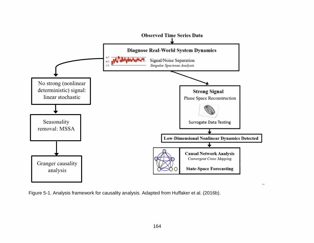
164
Figure 5-1. Analysis framework for causality analysis. Adapted from Huffaker et al. (2016b).

165
Figure 5-2. Characteristics of the study area after clustering analysis. a) The study area with 4 VDCs. b) Minimum,
median, maximum monthly Enhanced Vegetation Index (EVI2) time series per VDC. c) Map of the study area, with 99 communities and their average paving extent for the period 1987-2009. d) Area-weighted average paving extent per Vegetation Dynamics Cluster (0=road section associated with the community is unpaved,1=road section associated with the community is fully paved). VDCs are based on the adaptive dissimilarity index of EVI2. e) Average paving extent of the communities in each VDC, with an upward non-linear tendency from VDC 1 to 4. The tendency is a loess curve based on all average paving values.

166
Figure 5-3. Reconstructed time series, the signals, after Singular Spectrum Analysis.
EVI = Enhanced Vegetation Index 2, MAXT = maximum temperature, MEANT = mean temperature, MINT = minimum temperature, P = precipitation, PET = potential evapotranspiration, SM = soil moisture, AMO = Atlantic Multidecadal Oscillation, PDO = Pacific Decadal Oscillation, MEI = Multivariate ENSO Index.

167
Figure 5-4. Heat maps for the observed EVI2 (column 1), reconstructed EVI2 (column 3), and line plots for the observed
and reconstructed EVI2 (column 3) for VDC 1 (A), VDC 2 (B), VDC 3 (C) and VDC 4 (D). The heat maps have months along the x-axis (Jan – Dec) and years along the y-axis (1987 to 2009 from top to bottom).

168
Figure 5-5. Networks of cross-mapping skill (𝜌) of deterministic signals of EVI (𝜌 ≥ 0.65) per VDC, after testing for false
positives due to synchronicity. Bidirectional causality between minimum, mean, maximum temperature, precipitation, potential evapotransporation and soil moisture are not shown. EVI = Enhanced Vegetation Index 2, MAXT = maximum temperature, MEANT = mean temperature, MINT = minimum temperature, P = precipitation, PET = potential evapotranspiration, SM = soil moisture, AMO = Atlantic Multidecadal Oscillation, PDO = Pacific Decadal Oscillation, MEI = Multivariate ENSO Index.

169
CHAPTER 6
CONCLUSIONS
Main Findings
Scientific Findings
For an area in the Amazon that has been subject to road paving, this study
answered questions pertaining to resilience of a forest system in the face of
infrastructure development and increased anthropogenic influences and disturbances.
Based on existing literature on resilience, tipping points and road development impacts
the main hypothesis of this research was that “the identity of the coupled natural and
human system in the SW Amazon in the MAP area is affected by road paving, beyond
only deforestation, and different stable states exist.” While studies have already shown
that roads are key drivers of deforestation, less is known about forest degradation at
larger, regional scales. Degradation is generally an ill-defined concept (Putz and
Redford, 2010; Sasaki and Putz, 2009), and the definition of Putz and Redford (2010) is
adopted in this study: “[old growth] forests that lose their defining attributes (e.g.,
ancient trees, fauna, and coarse woody debris) through logging, market hunting,
wildfires, or invasion by exotic species, become degraded forest”. Note that this is
different from many global climate change agreements that generally refer to
degradation in terms of loss of canopy cover of carbon stock (Sasaki and Putz, 2009).
Degradation is affected not only by these spatial scales of road paving but also
different temporal scales: detecting change generally requires long time series, which
are not always available. Hence, the availability of multidisciplinary, long-term data for a
region in the SW Amazon that has been subject to highway paving provides the unique
opportunity to answer those questions. In particular, this study uniquely combines

170
available local socio-economic data, long-term remote sensing data, and information on
natural variables from re-analysis projects. We conducted data-driven research to draw
conclusions from characteristics from, and relationships between, data sets.
Considering that road paving is ongoing in coupled natural-human systems in many
parts of the world, results from this research are of interest to a wide audience, for
instance researchers on road ecology and disturbances, policy makers dealing with
environmental impact assessments and conservation issues, as well as international
organizations involved in conservation, climate change and financing of infrastructure
development.
This study focused on vegetation dynamics as an expression of the forest system
state. This is driven by the concept of ecosystem services in a coupled natural-human
system. Ecosystem services for both humans and nature are provided by the functions
of an ecosystem, and some examples of functions are water regulation, soil stability,
primary productivity, nutrient cycling. For a number of functions, such as the timing of
water and carbon cycles and primary productivity, phenology of vegetation (timing of
growth and senescence) plays an important role. Phenological ‘signatures’ of vegetation
(cycles and dynamics over time) and vegetation structure and composition are closely
related: different species will respond differently to certain conditions. Thus, a distinct
change in vegetation dynamics over time can imply a shift in vegetation composition
(especially if climatic conditions have not changed), or a change in timing of responses.
The latter also impacts ecosystem services. Ideally, long-term records of species
abundance and vegetation structure would allow quantification of road paving
degradation over time – as we consider these an attribute of the system. Unfortunately,

171
this information is not typically available, and if available, usually only locally. However,
spatio-temporal vegetation dynamics records based on remote sensing vegetation
indices provide a powerful proxy for analyses of changes from ongoing road paving.
The Enhanced Vegetation Index (EVI) was chosen as a suitable index, since it is known
to maintain its sensitivity under high biomass conditions (Huete et al., 2002), and it is
associated with Leaf Area Index and primary productivity (Cabello et al., 2012; Potter et
al., 2009), which are linked to ecosystem services. We used monthly EVI2 ((Z. Jiang et
al., 2008), as it provides long-term data from AVHRR reanalysis before 2000, and ‘true’
EVI from MODIS since then. AVHRR suffers more from cloud cover and other
atmospheric issues, so we anticipated the first period of our data set to have different
characteristics than the second period. This made it difficult to do a before/after road
paving analysis of each time series itself. Instead, we assembled monthly EVI2 with
other existing data for 99 communities along the Inter-Oceanic Highway that were
subject to paving at different points in time. To exclusively focus on dynamics, we only
used normalized time series of all variables.
The research was ordered around 3 sub-hypotheses to answer the main
hypothesis. First, we asked the question if we could find commonalities (shared
variance and shared behavior) in the monthly time series for EVI2 vegetation dynamics
spatially aggregated over each of the 99 local communities. All communities were
located along the Inter-Oceanic Highway that was paved during the period of study
(1987-2009), but paving started and finished at different times across communities. If
there was any effect from road paving on vegetation dynamics, clustering might group
communities together with a similar road paving history. After applying a time series

172
clustering technique based on values and behavior, we identified 4 Vegetation Cluster
Dynamics (VDCs) that we could associate with average road paving extent for the study
period. An analysis to identify the number of ‘states’ of average EVI2 over time (and a
breakpoint analysis) showed that there were differences between the clusters. Since the
number of states (dominant values in a histogram) is associated with dynamics, this
provided an early indication that dynamics differed between VDCs – as was the purpose
of the time series clustering technique. The existence of 4 VDCs confirmed our first sub-
hypothesis that “there are different states of vegetation dynamics associated with the
transitional states from unpaved to paved road development”. Available information on
soil and general forest types did not associate strongly with the clustering. The
dynamics of natural variables failed to cluster in the same way, a confirmation that there
was no single variable driving for the cluster results.
We used the cluster results to build unique Dynamic Factor Models for each
VDC. This was done to confirm the second hypothesis, that “the variables that explain
vegetation dynamics (in terms of variance) differ across a road paving gradient, with
human factors becoming more important”. DFMs use trends and variables as shared
explanatory factors across the VDCs and assign importance per community. The
strength of DFA is that it gives outputs for each community individually (spatial effects),
and it includes times series of observed covariates and auto-regressive (orthogonal)
trends (temporal effects). Trends represent unique shared variance between
communities, essentially indicating the existence of one or more explanatory variables
not included in the analysis. This analysis revealed a number of things, beyond simply
answering the sub-hypothesis. It showed that human factors, such as enforcement of

173
tenure rules, family density and travel time to market explained more of the variance in
vegetation dynamics under the paved condition. In addition, we also found that the
number of trends and the importance in explaining vegetation dynamics reduced from
the unpaved to the paved state. Thus, the variables included in the DFMs in the paved
state explain more of the vegetation dynamics.
Another important finding of this study was the fact that the change in importance
of trends and variables, and human and natural variables, was a complete switch for
each pair. When plotting this shift for all communities along their average road paving
extent, this switch happened at an average paving extent of 75% (for our 23-year
period), i.e. more or less between VDC 3 and 4. Lastly, by defining different DFMs for
each VDC, this method showed that the VDCs were not just different in the expression
of the vegetation dynamics, but potentially also in what drives the dynamics.
The last sub-hypothesis posed that “under the influence of road paving, the
causal network underlying vegetation dynamics would be disrupted and become
sparser”. This study looked at drivers deeper by applying (statistical) causality analyses.
The associated methods applied in this study are based on identifying deterministic
signals that represent a low-dimensional nonlinear deterministic system, i.e. an
attractor. Singular Spectrum Analysis (SSA) decomposes time series in components
from which a signal can be reconstructed – removing noise that would otherwise
complicate further analysis. The technique to determine causality, Convergent Cross
Mapping (CCM), is novel and is specifically suited for these low-dimensional nonlinear
deterministic systems, where linear approaches (such as Granger causality) do not
suffice for these systems because of the entanglement of information in time series. In

174
this analysis, the area-weighted averages of biophysical variables and EVI2 per cluster
were used, and the method was able to identify signals for each. After rigorous testing
for stationarity and determinism, VDC 1-3 were found suitable for CCM. For VDC 4 the
EVI2 signal was non-stationary. The resulting causality networks partly corroborated the
hypothesis and indicated differences in causal networks between VDCs. However, it
also showed an increase in causal connections from vegetation dynamics to natural
variables, instead of a decrease. Increased connectivity has been associated with less
resilience and a higher risk of collapse as any disturbances can travel and/or amplify
through the system (Gunderson and Holling, 2002). While causality between all
biophysical variables was strong and stayed the same across VDCs, the increase in
connectivity came from increased feedback from vegetation. Hence, while
vegetation/climate feedbacks and correlations have been found in previous studies
(Betts et al., 2004; Notaro et al., 2006), this study shows that the direction of these
relationships might vary locally or regionally, particularly in the presence of human
disturbance. In the undisturbed state, vegetation dynamics are driven by biophysical
variables, which themselves are not influenced by vegetation, but this changes for more
disturbed systems. The feedback from EVI2 implies that any further changes in
vegetation dynamics will impact biophysical variables too. The tight causal network also
suggests that methods used as early warnings for regime shifts (“critical slowing down”,
i.e. the reduced ability to recover from small perturbations) could be applied to only one,
or a few variables, but can serve as an early warning for the whole system. The fact that
the EVI2 signal was non-stationary implies that it was undergoing change over the
period of study. A suggestion here is that during road paving vegetation dynamics

175
indeed undergo change (increased connectivity from VDC 1-3) and eventually results in
a change of state (non-stationarity in VDC 4). Dynamic Factor Analysis also shows
shifts between the importance of trends versus variables, and human versus natural
variables between VDC 3 and 4.
Overall, this study confirms the first part of the main hypothesis: the identity of
the socio-ecological system in the SW Amazon in the MAP area is affected by road
paving, beyond only deforestation. However, the second part, that different stable states
exist, could not be conclusively answered. The non-stationary nature of the EVI2 signal
in VDC 4 in particular suggests this area is undergoing change.
While it was challenging to work with composite data (EVI2, socio-economical
and biological), it is of utmost importance that research on the development of the
products, and analysis on them, continues unabated. In order to find out how human
disturbances affect systems long-term, we need to do research on disturbances that
have already taken place; we cannot afford to only do research future or recent
disturbances. This poses challenges in obtaining data that go as far back as needed
(e.g. EVI2 data transformed from AVHRR, estimated socio-economic data), but with the
knowledge we gain from analyzing these data, while keeping uncertainties in mind, we
can contribute to adaptive management and the development of improved
methodologies and data sets. With the amount of undisturbed systems declining -
already in 1995, almost 75% of the habitable surface on earth was disturbed at least in
part by humans (Hannah et al., 1994; Sanderson et al., 2002), the time to understand
long-term effects is now.

176
Methodological Findings
After applying evaluation criteria to find the appropriate number of clusters, the
study found that seemingly similar criteria (the Dunn Index and Silhouette Width) still
gave different results. Besides the two criteria applied, there are a number of other
criteria available; some measure internal stability, others do external comparisons. So,
while the use of these criteria attempts to remove the subjectivity of clustering, it is
worth remembering that choosing the criteria also involves subjectivity. Combining
criteria that evaluate a similar measure is advisable in cluster studies.
The use of clusters made DFA application suitable, as this method seeks to
explain the shared variance among different locations throughout time. However, it did
make interpretation of the results more challenging, as analysis now included
comparisons between DFMs, not just within DFMs. Another challenge was the number
of variables included in these analyses, which limited the preferred approach of
assessing all possible combinations of variables. We consider the backwards
elimination method based on variance decomposition (partial R2) a good alternative, but
acknowledge there are other approaches to model specification that are just as valid.
Overall, we found DFA to be a useful tool in assessing areas undergoing change, with
each being at different points of the change process. While the uncovered relationships
do not imply causality, the analysis gave an indication that the VDCs are potentially
structurally different.
CCM has stringent requirements on the signals to which CCM can be applied, in
terms of stationarity and determinism. This proved to be limiting in analyzing VDC 4,
and highlighted that for areas actively undergoing change CCM might not be suitable. It
was encouraging that SSA uncovered signals for the time series, especially for EVI2,

177
which is considered noisy data. There is still a noise component that remains
unexplained, but we do not know how much of this is observation error and how much
process error. As with DFA, the number of variables included made this a time-
consuming analyses, since many of the pre-processing steps involve manual and visual
decisions and calculation settings. An advantage is that this allows the researcher to
become intimately involved with the data and the methods, gaining a better
understanding of their potential and their limitations. It does, however, also complicate
analyses of systems involving many variables.
The methods applied in this research are novel and take full advantage of
methods that have evolved over the years and current computational power. Compared
to what was possible years ago, it is an exciting time to do research on large long-term
data sets. The major challenge nowadays is evaluating applicability and the results that
are generated. The next section will touch on this and give recommendations for future
work.
Limitations And Future Research
When working with ecological data, issues with noisiness generally arise. This
study was no exception. This makes it difficult in some case to evaluate goodness-of-fit
of methods or model performance. In addition, remotely sensed products from tropical
areas are notorious for noisiness because of cloud cover and potential saturation at
high biomass values. While EVI2 purportedly solves the latter, there are still questions
around the validity of EVI2 representing vegetation. Since there is no clear answer to
this question as of yet, and the majority of studies and research articles support the use
of EVI2 for this purpose, it was deemed justified to use this variable in this study.

178
However, for future studies it would be interesting to compare EVI data and more locally
specific data, such as LiDAR, to find commonalities and anomalies.
The data that were used representing natural variables all come from reanalysis
studies. This means these are not actual measured values in most places. These
studies however use sophisticated methods to calculate and estimate values, and
several checks are in place to validate results. Considering the scarcity of data for areas
such as our study area, these data are invaluable to gain insight into processes in the
area. Since the methodologies applied in this research were time series analyses, there
are variables that would have been interesting to include, but that were not available as
a time series, e.g. general forest type or land cover. Future work can look at expanding
the existing database with additional time series.
In the DFA analysis, variables are assigned coefficients that can be interpreted
as the strength of the variable in explaining the response variable, though there is some
discussion in the scientific community about this. Certain conditions on collinearity need
to be met to make this true, and this is hardly ever the case. This is why this study uses
methods to counter this (calculation of Variance Inflation Factors, VIF), and also uses
the average semi-partial R2 for interpretation of results. It is recommended to generally
use two indicators (coefficients and semi-partial R2 ) to draw conclusions. Regarding the
inclusion of several trends in each model, part of the information contained in the trend
could refer to variables that we either failed to include or could not include due to time
series length. The could be variables such as cloudiness, fire, actual evapotranspiration
and human factors with a time series signature (food, timber, gold or Brazil nut prices,
selective logging intensity). There could also be a common observation error time

179
series, associated with typical remote sensing limitations in the tropics that are often
quite noisy.
While Cross Convergent Mapping is the most novel method to identify causality,
it bears repeating, from Chapter 5, that it is not possible to identify ‘true’ causality with
mathematical equations. Eventually CCM results still rely on some form of correlation,
albeit in a much more complex and nonlinear application. With that limitation said, CCM
is an innovative procedure with a solid foundation based on decades of research into
deterministic systems. Results from this research, as well as other studies (Lusch et al.,
2016; Sugihara et al., 2012), suggest that this method is preferred for causality analysis
over Granger causality analysis. Considering the earlier mentioned concerns about
EVI2 data, future research into characterizing EVI2 with CCM would provide interesting
insights into other phenological systems around the world. For example, comparing
results from more temperate regions and tropical regions might result in more clarity
about the potential error and noisiness of EVI in tropical areas. We found that extended
CCM offers exciting prospects, but yielded ambiguous results in some cases (e.g.
biophysical variables wrongly driving climate indices). This could be due to drivers
possibly acting indirectly (but strongly), so future research should focus on including
other variables that might play a role, such as cloudiness, wind, etc. Future work should
also include a closer look at the bi-directionality between some of the tightly coupled
biophysical variables: the results from the extended CCM include information that can
inform causal pathways. For the CCM procedure overall (including all pre-processing),
more research should lead to insights into cutoffs or significant values, as the ones

180
applied in this research are all derived from other methods, or are based on statistics
and common sense – but not necessarily experience.
This research only focuses on vegetation dynamics from a time series point of
view. While the results give us important insights into potential degradation, it does not
study detailed mechanisms of vegetation dynamics. Future research should focus on
mechanistic modeling of the system, to simulate the conditions this study in order to
gain more insight into underlying processes.
In general, limitations associated with this research stem from data and
methodology limitations. First, there will most likely be variables missing in the analyses,
which results in an “incomplete” picture of the system, leaving us to speculate about
certain findings (trends in FDA, certain causal relationships in CCM). We should also be
cautious about the actual data we have: vegetation indices are still only a proxy of
vegetation dynamics, and we make assumptions about its relationship with the real
world. Second, methodological constraints limit the certainty with which we can draw
conclusions. DFA finds relationships, but not necessarily causality. With CCM
uncovering statistical causality, we can make suggestions about real-world causality,
but these are still inferences. In addition, the stringent requirements on signals to apply
CCM to (stationarity, low-dimensional deterministic) excludes the application of this
approach to systems that are non-stationary and are undergoing change, and high-
dimensional systems. This is still a challenge, and a major topic for future research. This
research uncovered interesting potential relationships and potential change points, but a
large part of its contribution also lies in the evaluation of the usefulness and applicability
of advanced time series analyses to complex coupled natural and human systems.

181
Broader Impacts
This research has shown that, even in the absence of deforestation, road
construction potentially decreases the resilience of forest systems at larger regional
scales. While this research has not pinpointed the exact mechanisms, a relevant point is
that this disturbance and their drivers are often hidden due to the scale and complexity
of the effects. For example, on remote sensing images, these areas can still look
forested, but the structure and the dynamics might not be the same anymore. In
particular in CNH systems this is of importance, as ecosystem services are an integral
part of the connected system. The study shows that the change in forest dynamics
resulting from the road disturbance can potentially affect ecosystem services at much
larger scales through feedback mechanisms. For example, changes in temperature
regulation and carbon sequestration over large areas such as the Amazon could trigger
global hemispherical processes.
Overall, the findings of this research have implications for management of
(“undisturbed”) forest areas along roads. Larger protected areas along roads would be
recommended, with a focus on enforcement early on. Mostly though, the findings have
bearing on monitoring campaigns that can influence policy and management: ongoing
monitoring and analysis of data will highlight change or potential change and contribute
to adaptive management. Adaptive management will be required if indeed (the timing
of) ecosystem services changes in the area. It would thus be advisable to implement
monitoring programs that focus on vegetation dynamics on a long-term basis. This
could be done with existing remote sensing products such as MODIS, but ideally with
newer and more locally applicable technologies such as LiDAR, combined with new
high resolution remote sensing (e.g. WorldView or Europe’s Fluoresence Explorer,

182
FLEX). Research projects are underway to identify canopy structure, and even species,
from these technologies (Graves et al., 2016; Immitzer et al., 2012; Olivier et al., 2017;
Rybansky et al., 2016; Verrelst et al., 2015). As these technologies will become more
available as time goes by, regional (state) governments dealing with road paving
projects could be in a position to employ them. Efforts to educate local stakeholders on
these opportunities and transfer the results to improve management should be
sustained though long-term campaigns. We acknowledge this will be difficult for the
more general stakeholder population, considering the slow and long-term changes we
are considering here, and the more immediate, short-term pressing needs of the local
population. There are conservation organizations in the area though (e.g. the Amazon
Conservation Association) and research initiatives, which would be prominent
stakeholders, particularly for monitoring and transferring adaptive management
solutions.
Additionally, since causality analysis implies a strong link between biophysical
variables with increased paving, it is also advisable to monitor these closely. This is
usually easier than monitoring vegetation dynamics and many places already have
stations in place that monitor temperature and precipitation. However, ongoing analysis
of the data is key: other research has shown that time series characteristics undergo
changes, “critical slowing down”, when approaching tipping points (Dakos and
Bascompte, 2014; Scheffer et al., 2009). Considering the causal relationships, a change
in one (easily measured) variable could serve as a warning for the overall system. Note
that it would be useful in this context to have more insight into causal (mechanistic)
pathways mentioned earlier to ensure the appropriate variables are monitored.

183
Lastly, many road infrastructure projects in remote areas receive funding from
‘outside’ sources, such as development banks or international organizations (e.g. the
Inter-American Development Bank or the International Finance Corporation). This
research supports the urgent re-focusing by these organizations on forest degradation
in their environmental sustainability performance standards, especially focusing on
ongoing monitoring and analysis of vegetation dynamics and other socio-ecological
variables. While long-term effects are more complicated and costly to monitor than
immediate effects, the pay-offs are potentially greater. Preventing forest degradation will
conserve ecosystem services for the environment and humans for generations to come,
and should be part of corporate and organizational social responsibility.

184
APPENDIX A SUPPLEMENTARY MATERIALS FOR CHAPTER 4
Table A-1. Overview of communities included in the study.
Number Name km2 Country
X_1 3 Arroyos 124.6
Bolivia
X_2 Vera Cruz 104.3
X_3 Mukden 125.5
X_4 Extrema 87.8
X_5 Sena 222.5
X_6 Santa Rita 41.0
X_7 Santa María 117.5
X_8 San Antonio (Km. 60) 70.7
X_9 Santa Lucía 182.1
X_10 Trinchera 70.4
X_11 Litoral 7.5
X_12 San Luís 7.1
X_13 Nuevo Triunfo 0.0
X_14 Barzola (Villa Rosario) 0.9
X_15 Marapani 4.0
X_16 Santa Rosa de Abuná 32.2
X_17 Conquísta 27.1
X_18 Porvenir 7.7
X_19 Villa Rojas 5.9
X_20 Pontón 2.4
X_21 Santa Elena 12.7
X_23 Molienda 64.5
X_24 Irak 55.7
X_25 El Maty (San Antonio del) 160.0
X_26 Mandarino 115.8
X_27 Avaroa 39.1
X_28 Batraja 6.0
X_29 El Carmen 29.9
X_30 Karamano 5.0
X_31 Santa Lourdes 48.1
X_32 Primero de Mayo 14.0
X_33 Las Abejas 20.5
X_34 Jericó 5.0
X_35 Nueva Vida 22.3
X_36 Limera 0.0
X_37 Monterrey (Pando) 99.4

185
Table A-1. Continued.
Number Name km2 Country
X_38 C.N. Belgica 533.9
X_39 Villa Rocío 202.1
X_40 Union Progreso 29.8
X_41 Shiringayoc 72.1
Peru
X_42 Santo Domingo 4.8
X_43 Santa Rita Baja 33.4
X_44 Santa Rosa (Las Piedras) 46.4
X_45 San Bernardo 17.2
X_46 Villa Primavera 59.7
X_47 Planchon 113.9
X_48 Centro Poblado de Alegría 148.4
X_49 La Pastora 22.8
X_50 San Isidro De Chilin 75.6
X_51 Sudadero 170.4
X_52 Centro Poblado Menor de Mavila 196.5
X_53 Florida Baja 20.5
X_54 Florida Alta 42.4
X_55 A.C. Agraria Arca Pacahuara 81.4
X_56 Santa Rosa (Laberinto) 6.1
X_57 C.P. Alerta 46.1
X_58 Inaparí 26.4
X_59 Portillo 44.3
X_60 Loromayo 167.0
X_61 Virgen de la Candelaria 49.5
X_62 El Prado 14.8
X_63 Abeja 108.0
X_64 Nueva Esperanza 23.5
X_65 Chilina 15.1
X_66 San Antonio Abad 16.1
X_67 Ponalillo 17.5
X_68 La Merced 15.9
X_69 San Francisco de Asís 9.4
X_70 Monterrey (MDD) 83.5
X_71 Cachuela Alta 11.9
X_72 Otilia 5.5
X_73 Centro Cachuela 8.0
X_74 Asentamiento Humano El Tríunfo 0.8
X_75 Alto Libertad 52.5

186
Table A-1. Continued.
Number Name km2 Country
X_76 Seringal Filipinas 550.4
X_77 PA Benfica 57.0
X_78 PA Moreno Maia 227.9
X_79 PA Alcobras 107.1
X_80 PAE Remanso 431.2
X_81 PAE Santa Quiteria 693.1
X_82 PAD Quixada 529.9
X_83 PAE Chico Mendes 289.1
Brazil
X_84 PAE Porto Rico 118.9
X_85 PA Baixa Verde 50.7
X_86 PA Paraguassu 121.1
X_87 Sagarana 341.5
X_88 Seringal Sao Francisco do Iracema 505.2
X_89 Seringal Icuria 657.4
X_90 Seringal Independencia 121.7
X_91 Seringal Paraguacu 168.0
X_92 Polo Agroflorestal Brasileia 5.3
X_93 Polo Estrada da Borracha 2.3
X_94 Polo da Variante 3.4
X_95 PCA Helio Pimenta 1.4
X_96 PA Colibri 15.6
X_97 PA Vista Alegre 10.3
X_98 PA Limeira 22.8
X_99 KM 52 101.0
X_100 Seringal Sao Francisco 304.4
Abbreviations: PA/PAD = settlement projects, traditional projects of individual land concessions to small farmers PAE = Projectos de Assentamentos Agroextrativis (agro-extractive settlement projects, aimed at wild collector communities, mainly rubber-tappers and Brazil-nut collectors) PCA = projeto casulo (peri-urban settlement project for agricultural and ranching activities)

187
Table A-2. Statistical characteristics of monthly EVI2 time series (1982 – 2010) per VDC: mean (𝜇), median (M), standard deviation (𝜎), minimum (min) and maximum (max). n is the number of time series in a VDC. EVI2 is a combination of two-band and three-band Enhanced Vegetation Indexes, which are indexes calculated from surface reflectance measured by satellites. It represents vegetation dynamics and characteristics such as biomass and structure.
VDC 𝜇 M 𝜎 min max
1 (n=18) 0.50 - 0.53 0.50 - 0.54 0.06 - 0.08 0.23 - 0.38 0.65 - 0.75
2 (n=24) 0.42 - 0.53 0.43 - 0.53 0.05 - 0.08 0.14 - 0.35 0.56 - 0.76
3 (n=43) 0.49 - 0.54 0.50 - 0.54 0.05 - 0.08 0.05 - 0.35 0.65 - 0.72
4 (n=14) 0.44 - 0.54 0.45 - 0.53 0.06 - 0.08 0.20 - 0.38 0.58 - 0.73

188
Table A-3. Statistical properties of the monthly area-weighted time series of Candidate Explanatory Variables ν (January 1987 to December 2009, n=276) per VDC: mean ( ), median (M), standard deviation ( ), minimum (min) and
maximum (max). Human explanatory variables (νhum) Natural explanatory variables (νnat)
VDC ν M min max ν M min max
1 ENF 0.05 0.02 0.02 0.09 FOR 98 99 95 99
2 0.07 0.04 0.01 0.20 85 85 74 89 3 0.27 0.28 0.02 0.42 89 91 79 95 4 0.43 0.49 0.05 0.61 89 92 75 97 1 FAM 43 43 37 52 MAXT 31.6 31.5 28.3 34.5
2 159 153 127 221 30.0 30.0 25.9 33.5 3 169 168 150 193 30.9 30.8 27.6 33.9 4 184 184 179 191 31.6 31.5 28.8 34.3 1 FAMD 0.004 0.004 0.004 0.006 AVET 26.3 26.6 22.3 28.4
2 0.066 0.044 0.010 0.200 24.6 25.0 20.1 27.1 3 0.006 0.006 0.006 0.007 25.3 25.7 21.0 27.6 4 0.013 0.013 0.012 0.014 26.3 26.6 22.5 28.3 1 PNC 19,666 16,997 7,299 43,323 MINT 21.0 21.7 15.9 24.0 2 38,543 36,750 18,576 65,584 19.1 19.7 14.3 22.4 3 157,891 157,855 96,192 218,239 19.8 20.5 14.5 23.0 4 210,659 211,489 130,361 285,455 21.1 21.7 16.1 24.0 1 PNM 1,363 1,280 666 2,398 P 150 124 1 592 2 7,356 6,969 3,239 13,017 204 189 1 649 3 7,790 7,384 3,842 13,112 163 149 3 571 4 12,436 12,238 7,596 17,757 176 132 1 709 1 PAV 0.00 0.00 0.00 0.00 PET 101 101 75 131 2 0.09 0.00 0.00 0.82 108 107 77 136 3 0.37 0.27 0.00 0.88 99 99 76 126 4 0.65 0.85 0.04 0.98 92 92 71 114 1 TEN 0.63 1.00 0.10 1.00 SM 465 469 220 652 2 0.77 1.00 0.49 1.00 468 473 256 657 3 0.36 0.40 0.28 0.45 456 465 221 680 4 0.15 0.15 0.13 0.19 476 484 229 651 1 TTC 196 214 163 214 SR 306 305 300 315 2 95 95 79 95 141 140 123 154 3 246 234 184 313 107 103 83 130
m s
m m

189
Table A-3. Continued. Human explanatory variables (νhum) Natural explanatory variables (νnat)
VDC ν M min max ν M min max
4 126 109 106 162 66 64 36 94 1 TTM 40 40 40 40
2 25 25 19 25 3 47 47 43 49 4 62 59 59 69
m m

190
Table A-4. Lags applied to time series of candidate explanatory variables. The lags ( , in months) are based on the
highest cross-correlation coefficient ( ) between the lagged area-weighted average candidate explanatory
variable (X) and area-weighted average EVI2 time series (Y). The minus (-) sign indicates that the explanatory variable value occurs before the EVI2 value it has the highest correlation with. Text in bold highlights instances
where the cross-correlation is significant at .
VDC 1 VDC 2 VDC 3 VDC 4
Candidate Explanatory Variable
ENF Enforcement of tenure rules (0 to 1: with 0=least, 1=most)
-9 -0.01 -16 0.04 -21 -0.04 -13 0.14
FAM Number of families in the community (polygon) -15 0.06 -3 0.07 -15 -0.07 -13 -0.26
FAMD Family Density (families/km2) -21 -0.11 -4 0.06 0 -0.10 -6 -0.27
PGC Population growth at nearest state capital -15 0.03 -4 0.10 -15 0.05 -13 0.08
PGM Population growth at nearest market -15 0.05 -3 0.10 -21 -0.02 -13 0.06
PAV Paving (0 to 1, with 0=no paving, 1=fully paved) - - -21 -0.04 -21 -0.04 -13 0.20
TEN Percentage of deforestation allowed under tenure rules (0 to 1: e.g. 0.1=maximum of 10% deforestation allowed)
-16 -0.01 -4 -0.03 -21 0.04 -5 -0.12
TTC Travel time to capital (minutes) -21 0.03 0 0.07 -15 -0.10 -13 -0.20
TTM Travel time to nearest market (minutes) - - 0 0.06 0 -0.05 -5 -0.20
AVET Mean temperature (°C) -12 0.40 -12 0.35 -13 0.44 -13 0.40
FOR Forest area as percentage of polygon area -21 0.07 -4 -0.06 -21 0.05 0 0.06
MAXT Maximum temperature (°C) -13 0.33 -14 0.40 -14 0.43 -14 0.41
MINT Minimum temperature (°C) 0 0.40 -11 0.37 0 0.47 0 0.44
P Precipitation (mm) -4 -0.35 -17 -0.35 0 0.37 -1 0.34
PET Potential evapotranspiration (mm) -14 0.41 -14 0.45 -14 0.47 -15 0.43
SM Soil moisture (mm) -3 -0.39 -10 0.42 -4 -0.44 -4 -0.41
SR Species richness (alpha diversity) i -19 -0.22 0 -0.09 -13 -0.06 -1 -0.11
t
rXY t( )
±2
n= ±0.12 n = 276( )
t rXY t( ) t rXY t( ) t rXY t( ) t rXY t( )

191
Table A-5. Results of Variation Inflation Factor (VIF) analysis for explanatory variables included in dynamic factor analyses per VDC. All candidate explanatory variables (CEVs) with VIF > 10 are excluded. Lagged time series of the CEVs (as per Table A-3) are used in the VIF analysis.
Explanatory Variable VIF values
VDC 1 VDC 2 VDC 3 VDC 4
ENF Enforcement of tenure rules (0 to 1: with 0=least, 1=most) 2.09 1.96 5.34 FAMD Family Density (families/km2) 4.55 2.62 1.19 PAV Paving (0 to 1, with 0=no paving, 1=fully paved) 2.00* 7.58 TEN Percentage of deforestation allowed under tenure rules (0 to 1: e.g.
0.1=maximum of 10% deforestation allowed) 1.81 4.06 4.70
TTM Travel time to nearest market (minutes) 2.00* 6.30 2.60 FOR Forest area as percentage of polygon area 5.46 MAXT Maximum temperature (°C) 2.00 3.44 3.26 1.83 AVET Mean temperature (°C) 2.21 2.40 2.29 2.16 MINT Minimum temperature (°C) 2.24 3.17 3.22 2.98 P Precipitation (mm) 2.37 2.27 2.21 1.66 PET Potential evapotranspiration (mm) 3.70 6.55 4.66 3.40 SM Soil moisture (mm) 3.99 3.14 2.97 3.86 SR Species richness (alpha diversity) i 1.16 1.16 3.59
* Paving and travel time to market are constant over time and not included in further Dynamic Factor Analysis

192
Table A-6. Dynamic Factor Model (Model I, trends only) goodness-of-fit results of selected (best) models for individual communities.
VDC Community Ceff RMSE
1 X_5 0.59 0.65 X_6 0.62 0.60 X_7 0.86 0.38 X_8 0.77 0.47 X_9 0.86 0.37 X_17 0.60 0.63 X_21 0.68 0.57 X_24 0.85 0.39 X_25 0.87 0.35 X_26 0.81 0.44 X_27 0.87 0.36 X_28 0.75 0.50 X_29 0.71 0.54 X_32 0.50 0.71 X_33 0.48 0.72 X_34 0.74 0.51 X_35 0.63 0.60 X_37 0.75 0.50 2 X_39 0.87 0.36 X_40 0.53 0.70 X_41 0.87 0.36 X_42 0.90 0.31 X_43 0.56 0.67 X_44 0.74 0.52 X_45 0.61 0.64 X_47 0.92 0.29 X_48 0.91 0.30 X_49 0.61 0.63 X_51 0.86 0.38 X_52 0.89 0.33 X_53 0.49 0.73 X_54 0.98 0.15 X_56 0.54 0.69 X_60 0.53 0.70 X_61 0.74 0.51 X_62 1.00 0.01 X_70 0.89 0.33 X_71 0.59 0.65 X_72 0.64 0.61 X_73 1.00 0.01 X_74 0.68 0.58 X_75 0.91 0.30

193
Table A-6. Continued.
VDC Community Ceff RMSE
3 X_1 0.89 0.34 X_2 0.79 0.46 X_3 0.79 0.46 X_4 0.87 0.36 X_10 0.57 0.67 X_11 0.52 0.70 X_12 0.72 0.54 X_13 0.72 0.53 X_14 0.72 0.53 X_15 0.63 0.61 X_18 0.57 0.66 X_19 0.66 0.58 X_20 0.72 0.53 X_23 0.77 0.48 X_30 0.56 0.66 X_31 0.63 0.62 X_36 0.67 0.58 X_38 0.91 0.31 X_46 0.74 0.51 X_50 0.78 0.47 X_55 0.75 0.50 X_57 0.68 0.57 X_58 0.80 0.45 X_59 1.00 0.02 X_63 0.90 0.32 X_64 0.63 0.62 X_65 0.72 0.53 X_66 0.67 0.58 X_67 0.61 0.63 X_68 0.79 0.46 X_69 1.00 0.02 X_76 0.88 0.35 X_81 0.85 0.39 X_82 0.88 0.35 X_83 0.79 0.46 X_84 0.81 0.44 X_86 0.72 0.54 X_87 0.82 0.43 X_89 0.84 0.41 X_91 0.85 0.39 X_92 0.70 0.55 X_99 0.78 0.47 X_100 0.91 0.31

194
Table A-6. Continued.
VDC Community Ceff RMSE
4 X_16 0.29 0.85 X_77 0.68 0.57 X_78 0.81 0.44 X_79 0.72 0.54 X_80 0.81 0.44 X_85 0.68 0.57 X_88 0.92 0.29 X_90 0.81 0.45 X_93 0.56 0.66 X_94 0.50 0.72 X_95 0.56 0.66 X_96 0.70 0.55 X_97 0.65 0.60 X_98 0.66 0.58

195
Table A-7. Average relative importance of trends and explanatory variables in dynamic factor analyses (Model II, trends and explanatory variables) simulating EVI2. Backward selection is applied; the variables with the lowest mean relative importance (LMG) are eliminated one by one until the Bayesian Information Criterion (BIC) reaches its lowest point. Italic = selected models.
VDC 1 VDC 2 VDC 3 VDC 4 EV LMG
(mean) BIC EV LMG
(mean) BIC EV LMG
(mean) BIC EV LMG
(mean) BIC
γ1 0.21 9994 γ1 0.17 10390 γ4 0.27 19010 γ1 0.19 8100 γ2 0.19 γ4 0.14 γ1 0.15 FAMD 0.16 γ4 0.19 γ3 0.12 γ2 0.10 γ3 0.16 ENF 0.06 γ2 0.10 γ6 0.08 TTM 0.10 AVET 0.05 TTM 0.07 PET 0.05 γ2 0.06 MINT 0.04 PAV 0.06 γ5 0.05 PET 0.05 γ3 0.04 γ7 0.04 SM 0.04 MINT 0.05 PET 0.04 PET 0.04 MINT 0.04 AVET 0.05 FOR 0.04 γ6 0.04 FAMD 0.04 MAXT 0.05 SR 0.04 SM 0.04 AVET 0.04 P 0.04 SM 0.03 MAXT 0.04 MAXT 0.04 ENF 0.04 FAMD 0.03 γ5 0.03 γ3 0.03 SM 0.03 MAXT 0.02 P 0.03 P 0.03 TEN 0.02 P 0.02 MINT 0.02 TEN 0.02 AVET 0.02 SR 0.02 SR 0.02 ENF 0.01 TEN 0.01 γ1 0.21 9958 γ1 0.19 10322 γ3 0.28 18900 γ1 0.19 8076 γ2 0.20 γ7 0.14 γ1 0.15 FAMD 0.19 γ4 0.19 γ3 0.13 γ2 0.10 γ2 0.16 ENF 0.05 γ2 0.10 γ6 0.08 TTM 0.09 AVET 0.05 PAV 0.06 γ5 0.05 γ3 0.06 MINT 0.05 TTM 0.06 PET 0.05 PET 0.05 PET 0.04 γ4 0.05 MINT 0.04 MINT 0.05 γ3 0.04 γ6 0.05 SM 0.04 AVET 0.05 SR 0.04 PET 0.04 MAXT 0.04 MAXT 0.05

196
Table A-7. Continued. VDC 1 VDC 2 VDC 3 VDC 4 EV LMG
(mean) BIC EV LMG
(mean) BIC EV LMG
(mean) BIC EV LMG
(mean) BIC
SM 0.04 SR 0.03 AVET 0.04 ENF 0.05 FOR 0.03 MAXT 0.03 FAMD 0.04 P 0.04 MAXT 0.02 SM 0.03 γ4 0.03 SM 0.03 FAMD 0.02 γ5 0.03 P 0.03 P 0.02 TEN 0.02 MINT 0.02 SR 0.02 AVET 0.02 γ1 0.21 9923 γ1 0.17 10266 γ3 0.28 18817 FAMD 0.20 8054 γ2 0.19 γ7 0.14 γ1 0.17 γ2 0.20 γ4 0.19 γ3 0.13 γ2 0.10 γ1 0.16 FOR 0.06 γ2 0.09 γ6 0.08 TTM 0.08 ENF 0.06 PAV 0.06 PET 0.05 PET 0.06 AVET 0.05 TTM 0.05 γ5 0.04 MINT 0.06 MINT 0.05 γ6 0.05 MINT 0.04 γ3 0.05 PET 0.04 γ4 0.05 SM 0.04 AVET 0.05 γ3 0.04 SR 0.05 MAXT 0.04 MAXT 0.05 SR 0.04 PET 0.04 AVET 0.04 ENF 0.05 SM 0.04 SM 0.04 FAMD 0.04 P 0.05 MAXT 0.02 MAXT 0.04 γ4 0.03 γ5 0.03 P 0.03 P 0.03 TEN 0.02 MINT 0.03 γ1 0.22 9896 γ1 0.20 10244 γ3 0.27 18695 γ1 0.21 8056 γ4 0.19 γ4 0.16 γ1 0.17 FAMD 0.21 γ2 0.18 γ3 0.14 γ2 0.10 γ2 0.16 FOR 0.08 γ2 0.10 γ6 0.08 PET 0.07 AVET 0.06 PAV 0.06 FAMD 0.06 MINT 0.07 MINT 0.05 TTM 0.06 γ5 0.05 γ3 0.07 ENF 0.05 γ7 0.05 PET 0.05 TTM 0.06

197
Table A-7. Continued. VDC 1 VDC 2 VDC 3 VDC 4 EV LMG
(mean) BIC EV LMG
(mean) BIC EV LMG
(mean) BIC EV LMG
(mean) BIC
PET 0.05 γ5 0.05 MINT 0.04 AVET 0.06 SM 0.04 PET 0.04 SM 0.04 MAXT 0.05 SR 0.04 SM 0.04 MAXT 0.04 ENF 0.05 γ3 0.04 MAXT 0.04 AVET 0.04 γ6 0.03 γ4 0.03 P 0.02 P 0.03 SR 0.02 γ1 0.20 9939 γ1 0.20 10262 γ3 0.27 18590 γ3 0.19 γ3 0.15 γ1 0.17 γ2 0.17 γ6 0.14 γ2 0.10 FOR 0.13 γ2 0.10 γ6 0.08 AVET 0.06 PAV 0.06 FAMD 0.06 MINT 0.05 TTM 0.06 PET 0.05 SR 0.05 γ5 0.05 γ5 0.05 PET 0.05 PET 0.05 SM 0.05 ENF 0.04 SM 0.04 MINT 0.05 SM 0.04 γ7 0.04 AVET 0.04 MAXT 0.04 MAXT 0.04 γ4 0.03 γ4 0.03 SR 0.02 γ3 0.30 18664 γ4 0.18 γ2 0.09 γ1 0.09 FAMD 0.06 PET 0.05 SM 0.05

198
Table A-7. Continued. VDC 1 VDC 2 VDC 3 VDC 4 EV LMG
(mean) BIC EV LMG
(mean) BIC EV LMG
(mean) BIC EV LMG
(mean) BIC
MINT 0.05 AVET 0.04 MAXT 0.04 γ5 0.04

199
Table A-8. Dynamic Factor Model (Model II, trends and explanatory variables) goodness-of-fit results of selected (best) models for individual communities.
VDC Community Ceff RMSE
1 X_5 0.61 0.63 X_6 0.62 0.60 X_7 0.86 0.37 X_8 0.78 0.47 X_9 0.87 0.36 X_17 0.63 0.61 X_21 0.68 0.57 X_24 0.87 0.36 X_25 0.88 0.35 X_26 0.83 0.41 X_27 0.81 0.44 X_28 0.75 0.50 X_29 0.74 0.51 X_32 0.51 0.70 X_33 0.49 0.71 X_34 0.75 0.50 X_35 0.67 0.58 X_37 0.77 0.48 2 X_39 0.87 0.36 X_40 0.55 0.69 X_41 0.88 0.34 X_42 0.91 0.30 X_43 0.58 0.65 X_44 0.74 0.52 X_45 0.62 0.63 X_47 0.93 0.27 X_48 0.91 0.30 X_49 0.62 0.62 X_51 0.86 0.38 X_52 0.90 0.32 X_53 0.52 0.70 X_54 0.98 0.15 X_56 0.56 0.68 X_60 0.58 0.66 X_61 0.79 0.47 X_62 1.00 0.01 X_70 0.90 0.33 X_71 0.62 0.63 X_72 0.68 0.58 X_73 1.00 0.01 X_74 0.68 0.57

200
Table A-8. Continued.
VDC Community Ceff RMSE
X_75 0.91 0.30 3 X_1 0.89 0.33 X_2 0.81 0.44 X_3 0.80 0.45 X_4 0.87 0.36 X_10 0.59 0.65 X_11 0.61 0.63 X_12 0.76 0.49 X_13 0.73 0.52 X_14 0.72 0.53 X_15 0.67 0.58 X_18 0.58 0.65 X_19 0.67 0.58 X_20 0.71 0.54 X_23 0.80 0.45 X_30 0.57 0.65 X_31 0.64 0.61 X_36 0.68 0.57 X_38 0.91 0.31 X_46 0.75 0.50 X_50 0.78 0.47 X_55 0.78 0.48 X_57 0.69 0.56 X_58 0.81 0.45 X_59 1.00 0.02 X_63 0.91 0.31 X_64 0.64 0.61 X_65 0.74 0.51 X_66 0.67 0.58 X_67 0.63 0.61 X_68 0.79 0.46 X_69 1.00 0.02 X_76 0.87 0.37 X_81 0.85 0.39 X_82 0.88 0.36 X_83 0.80 0.45 X_84 0.82 0.43 X_86 0.75 0.50 X_87 0.82 0.43 X_89 0.84 0.40 X_91 0.84 0.40 X_92 0.70 0.55 X_99 0.80 0.45

201
Table A-8. Continued.
VDC Community Ceff RMSE
X_100 0.92 0.29 4 X_16 0.33 0.83 X_77 0.70 0.55 X_78 0.81 0.43 X_79 0.72 0.54 X_80 0.81 0.44 X_85 0.68 0.57 X_88 0.92 0.28 X_90 0.84 0.40 X_93 0.61 0.62 X_94 0.49 0.72 X_95 0.59 0.65 X_96 0.74 0.52 X_97 0.66 0.60 X_98 0.66 0.59

202
Table A-9. Beta coefficients (weightings, β) of the explanatory variables for the selected Dynamic Factor Models II (trends and explanatory variables).
VDC 1 βENF βFAMD βPAV βTEN βTTM βFOR βMAXT βAVET βMINT βP βPET βSM βSR
X_5 0.35 0.37 0.23 -0.01 -0.01 -0.29 -0.10
X_6 0.32 0.59 0.05 0.12 0.01 -0.31 -0.14
X_7 0.17 0.57 0.12 0.18 0.21 -0.09 -0.19
X_8 0.32 0.68 0.10 0.17 -0.01 -0.24 -0.18
X_9 0.40 0.67 0.04 0.23 0.27 -0.09 -0.15
X_17 0.46 0.48 0.19 0.10 0.07 -0.12 -0.09
X_21 0.60 0.65 0.11 0.14 0.17 0.06 -0.17
X_24 1.02 0.61 0.21 0.20 0.11 0.14 -0.21
X_25 0.72 0.59 0.22 0.15 0.07 0.01 -0.24
X_26 0.84 0.78 0.17 0.07 0.08 0.05 -0.24
X_27 1.37 0.87 0.08 0.18 -0.05 0.16 -0.34
X_28 0.49 0.27 0.26 0.13 0.12 0.20 -0.13
X_29 0.87 0.66 0.15 0.05 0.28 0.09 -0.16
X_32 0.45 0.58 0.17 0.21 0.05 -0.02 -0.19
X_33 0.55 0.55 0.26 0.15 0.13 0.19 -0.15
X_34 0.66 0.41 0.14 0.22 0.10 0.10 -0.16
X_35 0.65 0.60 0.04 0.27 0.16 0.05 -0.12
X_37 0.88 0.76 0.23 0.06 0.26 0.27 -0.13
VDC 2
X_39 0.96 1.31 -0.03 -0.10 0.15 0.19 0.11
X_40 2.00 1.12 0.03 -0.01 0.33 -0.20 -0.15
X_41 1.21 1.52 -0.03 -0.04 0.24 0.11 0.04
X_42 -0.76 -0.62 0.06 0.07 0.05 -0.09 -0.22
X_43 1.86 0.80 0.16 -0.06 0.03 0.02 -0.19
X_44 0.86 1.32 0.04 -0.11 -0.02 0.17 0.12
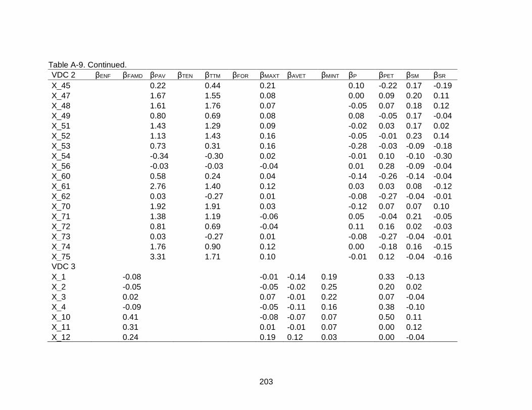
203
Table A-9. Continued.
VDC 2 βENF βFAMD βPAV βTEN βTTM βFOR βMAXT βAVET βMINT βP βPET βSM βSR
X_45 0.22 0.44 0.21 0.10 -0.22 0.17 -0.19
X_47 1.67 1.55 0.08 0.00 0.09 0.20 0.11
X_48 1.61 1.76 0.07 -0.05 0.07 0.18 0.12
X_49 0.80 0.69 0.08 0.08 -0.05 0.17 -0.04
X_51 1.43 1.29 0.09 -0.02 0.03 0.17 0.02
X_52 1.13 1.43 0.16 -0.05 -0.01 0.23 0.14
X_53 0.73 0.31 0.16 -0.28 -0.03 -0.09 -0.18
X_54 -0.34 -0.30 0.02 -0.01 0.10 -0.10 -0.30
X_56 -0.03 -0.03 -0.04 0.01 0.28 -0.09 -0.04
X_60 0.58 0.24 0.04 -0.14 -0.26 -0.14 -0.04
X_61 2.76 1.40 0.12 0.03 0.03 0.08 -0.12
X_62 0.03 -0.27 0.01 -0.08 -0.27 -0.04 -0.01
X_70 1.92 1.91 0.03 -0.12 0.07 0.07 0.10
X_71 1.38 1.19 -0.06 0.05 -0.04 0.21 -0.05
X_72 0.81 0.69 -0.04 0.11 0.16 0.02 -0.03
X_73 0.03 -0.27 0.01 -0.08 -0.27 -0.04 -0.01
X_74 1.76 0.90 0.12 0.00 -0.18 0.16 -0.15
X_75 3.31 1.71 0.10 -0.01 0.12 -0.04 -0.16
VDC 3
X_1 -0.08 -0.01 -0.14 0.19 0.33 -0.13
X_2 -0.05 -0.05 -0.02 0.25 0.20 0.02
X_3 0.02 0.07 -0.01 0.22 0.07 -0.04
X_4 -0.09 -0.05 -0.11 0.16 0.38 -0.10
X_10 0.41 -0.08 -0.07 0.07 0.50 0.11
X_11 0.31 0.01 -0.01 0.07 0.00 0.12
X_12 0.24 0.19 0.12 0.03 0.00 -0.04

204
Table A-9. Continued.
VDC 3 βENF βFAMD βPAV βTEN βTTM βFOR βMAXT βAVET βMINT βP βPET βSM βSR
X_13 0.25 0.17 0.10 0.03 -0.04 -0.31
X_14 0.42 0.17 0.07 0.02 -0.09 -0.24
X_15 0.47 -0.02 0.08 -0.14 0.18 -0.18
X_18 0.38 0.01 -0.01 0.03 0.05 -0.28
X_19 0.34 0.21 0.06 -0.06 -0.21 -0.40
X_20 0.28 0.16 0.09 0.06 -0.07 -0.26
X_23 0.10 -0.14 -0.11 0.18 0.44 -0.03
X_30 0.33 0.03 -0.10 0.08 0.47 0.10
X_31 0.44 0.10 0.06 -0.01 0.11 0.05
X_36 0.26 0.05 0.02 0.09 0.10 -0.18
X_38 -0.28 0.12 0.05 0.09 0.04 -0.15
X_46 -0.32 0.22 0.07 0.13 -0.19 -0.16
X_50 -0.18 0.03 0.00 0.15 0.13 -0.11
X_55 -0.17 0.17 -0.04 -0.04 0.11 -0.20
X_57 -0.10 0.13 0.04 0.16 -0.07 -0.12
X_58 -0.20 0.26 0.18 -0.04 -0.42 -0.32
X_59 -0.03 0.00 -0.06 -0.07 0.09 -0.01
X_63 -0.21 0.12 -0.07 0.19 0.05 -0.08
X_64 -0.17 0.19 0.13 -0.16 -0.09 -0.26
X_65 -0.12 0.22 -0.05 0.01 -0.03 -0.24
X_66 -0.24 0.17 0.01 0.05 -0.21 -0.18
X_67 -0.24 0.24 -0.03 0.08 -0.05 -0.11
X_68 -0.16 0.03 -0.13 0.18 0.13 -0.08
X_69 -0.03 0.00 -0.06 -0.07 0.09 -0.01
X_76 0.57 -0.07 -0.02 0.17 0.27 0.00
X_81 0.01 0.10 0.14 0.14 0.03 -0.14

205
Table A-9. Continued.
VDC 3 βENF βFAMD βPAV βTEN βTTM βFOR βMAXT βAVET βMINT βP βPET βSM βSR
X_82 0.35 0.19 0.13 0.03 -0.15 -0.27
X_83 0.45 -0.12 -0.03 0.17 0.37 0.01
X_84 0.49 0.14 0.02 0.05 0.03 -0.19
X_86 -0.24 0.25 0.04 0.18 -0.21 -0.09
X_87 0.62 0.03 -0.03 0.11 0.16 0.04
X_89 -0.13 0.13 0.07 0.16 0.17 0.00
X_91 -0.09 0.14 0.14 0.11 0.03 -0.08
X_92 0.46 0.17 0.12 -0.06 -0.18 -0.35
X_99 0.44 0.06 0.12 0.05 0.25 -0.05
X_100 -0.34 0.24 0.06 0.12 -0.14 -0.13
VDC 4
X_16 -0.44 -0.66 -0.36 0.11 -0.01 0.28 0.16 -0.05
X_77 -0.73 -1.06 -0.95 0.25 0.08 0.01 0.06 0.14
X_78 -0.53 -1.33 -0.46 0.13 -0.01 0.13 0.24 0.15
X_79 -0.51 -1.11 -0.61 0.19 -0.02 0.17 0.14 0.13
X_80 -0.45 -1.07 -0.33 0.17 0.00 0.26 0.13 0.12
X_85 -0.54 -0.81 -0.91 0.19 0.13 0.05 0.02 0.21
X_88 -0.33 -0.97 -0.14 0.17 0.09 0.14 0.10 0.09
X_90 -0.26 -0.84 -0.09 0.18 0.01 0.18 0.17 -0.10
X_93 -0.62 -0.86 -0.65 0.15 0.09 0.08 0.11 0.29
X_94 -0.52 -0.81 -0.75 0.09 0.14 0.08 0.02 0.13
X_95 -0.48 -1.00 -0.67 0.20 0.02 0.18 0.04 0.05
X_96 -0.63 -0.91 -1.07 0.15 0.08 0.08 -0.09 0.26
X_97 -0.52 -1.35 -0.32 0.13 0.04 0.11 0.05 0.19
X_98 -0.59 -1.01 -0.79 0.15 0.08 0.05 0.15 0.18

206
Table A-10. Factor loadings (weightings, α) of the trends for the selected Dynamic Factor Models II (trends and explanatory variables), for each community.
α1 α2 α3 α4 α5 α6 α7
VDC 1
X_5 0.54 0.32 -0.06 0.25
X_6 0.09 0.53 -0.12 0.11
X_7 0.23 0.58 0.03 0.25
X_8 0.20 0.62 -0.08 0.14
X_9 0.29 0.52 -0.04 0.35
X_17 0.60 0.30 -0.10 0.17
X_21 0.19 0.24 -0.07 0.63
X_24 0.78 0.22 -0.29 0.45
X_25 0.68 0.35 -0.18 0.42
X_26 0.56 0.35 -0.14 0.60
X_27 0.30 0.21 -0.54 0.31
X_28 0.77 0.18 -0.08 0.29
X_29 0.35 0.15 -0.18 0.69
X_32 0.34 0.40 -0.10 0.13
X_33 0.31 0.21 -0.08 0.46
X_34 0.71 0.22 -0.12 0.48
X_35 0.18 0.17 -0.09 0.63
X_37 0.51 0.28 -0.10 0.60
VDC 2
X_39 0.71 0.12 -0.27 0.14 0.01 -0.32 0.09
X_40 0.33 0.57 -0.28 0.03 0.05 0.04 0.01
X_41 0.69 0.08 -0.07 0.23 0.01 -0.42 0.05
X_42 0.17 0.24 -1.00 0.13 -0.03 0.04 0.00
X_43 0.20 0.60 -0.37 0.09 0.02 0.03 -0.04

207
Table A-10. Continued.
α1 α2 α3 α4 α5 α6 α7
X_44 0.75 0.07 -0.18 0.17 0.02 -0.12 0.12
X_45 0.47 0.16 -0.50 0.17 -0.06 -0.06 -0.04
X_47 0.81 0.33 -0.15 0.11 -0.01 0.20 -0.09
X_48 0.86 0.23 -0.08 0.12 0.02 0.09 0.00
X_49 0.40 0.12 -0.31 0.64 0.10 -0.09 -0.02
X_51 0.69 0.27 -0.21 0.27 -0.04 0.14 -0.15
X_52 0.78 0.12 -0.13 0.18 0.00 -0.19 0.04
X_53 0.09 0.31 -0.36 0.26 -0.04 -0.20 0.12
X_54 0.21 0.33 -1.04 0.09 0.04 0.01 0.01
X_56 0.26 0.19 -0.60 0.39 0.07 -0.08 0.10
X_60 0.17 0.33 -0.39 0.31 0.03 -0.11 0.37
X_61 0.23 0.75 -0.31 0.20 0.05 -0.06 0.08
X_62 0.18 0.02 -0.18 1.28 -0.09 -0.04 0.12
X_70 0.87 0.32 -0.18 0.09 0.06 0.12 0.06
X_71 0.59 0.22 -0.20 0.38 -0.01 0.12 -0.13
X_72 0.45 0.16 -0.31 0.67 0.19 0.01 0.06
X_73 0.18 0.02 -0.18 1.28 -0.09 -0.04 0.12
X_74 0.16 0.28 0.05 0.60 0.05 -0.02 -0.32
X_75 0.20 0.84 -0.07 0.05 -0.06 -0.04 -0.02
VDC 3
X_1 0.75 0.19 0.28 0.01 0.01 0.17
X_2 0.71 0.30 0.31 -0.12 -0.07 0.26
X_3 0.48 0.45 0.40 -0.13 -0.08 0.34
X_4 0.76 0.20 0.26 0.02 0.00 0.18
X_10 0.37 0.08 0.56 -0.06 -0.05 -0.13
X_11 0.53 0.26 0.48 -0.22 -0.08 0.31

208
Table A-10. Continued.
α1 α2 α3 α4 α5 α6 α7
X_12 0.06 0.08 0.45 0.02 0.28 0.16
X_13 0.20 0.19 0.49 0.11 0.09 0.15
X_14 0.17 0.18 0.62 0.10 -0.01 0.27
X_15 0.26 0.09 0.63 0.05 -0.10 0.45
X_18 0.27 0.04 0.52 0.13 0.05 0.16
X_19 0.10 0.12 0.54 0.18 0.00 0.36
X_20 0.23 0.10 0.53 0.20 0.00 0.22
X_23 0.61 0.18 0.31 -0.23 -0.04 0.40
X_30 0.34 0.18 0.45 -0.13 -0.06 -0.18
X_31 0.30 0.03 0.59 -0.09 0.09 0.01
X_36 0.23 0.24 0.52 -0.03 0.05 0.30
X_38 0.40 0.63 0.26 -0.04 0.03 0.43
X_46 0.49 0.48 0.23 0.06 0.02 0.55
X_50 0.59 0.25 0.26 0.08 0.12 0.43
X_55 0.41 0.36 0.23 0.04 0.01 0.94
X_57 0.60 0.31 0.27 0.03 -0.04 0.49
X_58 0.24 0.36 0.29 0.12 0.25 0.52
X_59 0.35 0.22 0.27 -0.24 -0.07 1.89
X_63 0.75 0.20 0.25 0.12 0.07 0.55
X_64 0.20 0.41 0.34 0.17 0.08 0.56
X_65 0.44 0.31 0.27 0.06 0.04 0.78
X_66 0.41 0.22 0.19 0.08 0.14 0.87
X_67 0.58 0.17 0.22 0.19 0.07 0.42
X_68 0.73 0.20 0.23 0.06 0.12 0.38
X_69 0.35 0.22 0.27 -0.24 -0.07 1.89
X_76 0.25 0.26 0.70 -0.24 -0.08 0.14

209
Table A-10. Continued.
α1 α2 α3 α4 α5 α6 α7
X_81 0.27 0.45 0.47 0.05 0.04 0.31
X_82 0.12 0.28 0.65 0.12 0.00 0.37
X_83 0.34 0.23 0.61 -0.19 -0.02 -0.02
X_84 0.24 0.13 0.66 -0.08 0.08 0.10
X_86 0.25 0.61 0.32 0.08 -0.05 0.60
X_87 0.10 0.29 0.71 -0.29 -0.06 0.28
X_89 0.27 0.53 0.34 -0.07 0.01 0.27
X_91 0.31 0.57 0.38 -0.02 0.03 0.13
X_92 0.05 0.13 0.61 0.10 0.02 0.25
X_99 0.07 0.31 0.66 -0.04 -0.05 0.13
X_100 0.38 0.70 0.26 -0.01 0.03 0.31
VDC 4
X_16 0.27 0.26 0.00
X_77 0.21 0.63 0.00
X_78 0.40 0.58 -0.07
X_79 0.41 0.54 0.00
X_80 0.58 0.34 -0.01
X_85 0.26 0.57 0.06
X_88 0.72 0.18 -0.01
X_90 0.77 0.15 0.01
X_93 0.10 0.54 -0.04
X_94 0.28 0.46 0.05
X_95 0.30 0.56 0.01
X_96 0.19 0.67 0.08
X_97 0.18 0.58 -0.13
X_98 0.17 0.59 0.01
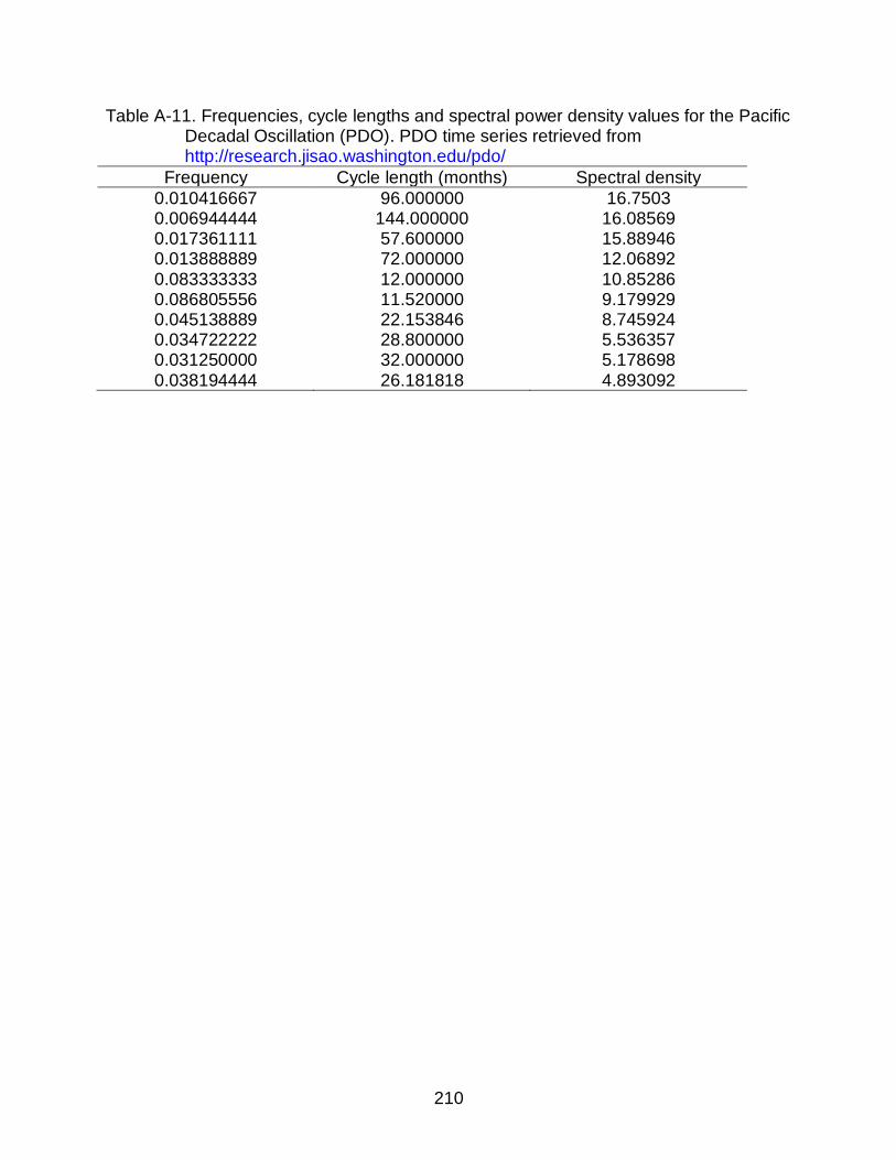
210
Table A-11. Frequencies, cycle lengths and spectral power density values for the Pacific Decadal Oscillation (PDO). PDO time series retrieved from http://research.jisao.washington.edu/pdo/
Frequency Cycle length (months) Spectral density
0.010416667 96.000000 16.7503 0.006944444 144.000000 16.08569 0.017361111 57.600000 15.88946 0.013888889 72.000000 12.06892 0.083333333 12.000000 10.85286 0.086805556 11.520000 9.179929 0.045138889 22.153846 8.745924 0.034722222 28.800000 5.536357 0.031250000 32.000000 5.178698 0.038194444 26.181818 4.893092
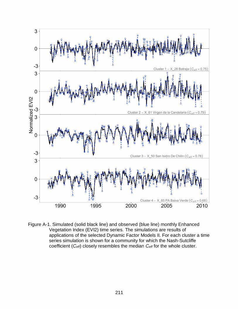
211
Figure A-1. Simulated (solid black line) and observed (blue line) monthly Enhanced Vegetation Index (EVI2) time series. The simulations are results of applications of the selected Dynamic Factor Models II. For each cluster a time series simulation is shown for a community for which the Nash-Sutcliffe coefficient (Ceff) closely resembles the median Ceff for the whole cluster.

212
APPENDIX B SUPPLEMENTARY MATERIALS FOR CHAPTER 5
Data and code for calculations (including explanations) can be found on 10.6084/m9.figshare.c.3933388 Table B-1. Cycle lengths (months) used to set the window length in Singular Spectrum
Analysis (based on spectral density results).
Cycle lengths (m) VDC EVI MAXT MINT P PET SM SR AMO PDO MEI
1 12 12 12 12 12 12 32 12 12 12 2 12 12 12 12 12 12 12 3 12 12 12 12 12 12 12 4 12 12 12 12 12 12 12

213
Table B-2. Weighted adjacency matrices EVI MAXT MEANT MINT P PET SM AMO PDO MEI
VDC 1 EVI 0.99 0.98 0.96 0.97 1.00 0.99 0.75 0.31 -0.25 MAXT 0.99 0.98 0.96 0.97 1.00 0.99 0.92 0.46 -0.13 MEANT 0.99 0.98 0.97 0.95 0.99 0.99 0.11 0.25 -0.21 MINT 0.95 0.87 0.97 0.93 0.88 0.96 -0.06 0.15 0.01 P 0.99 0.99 0.99 0.97 0.99 0.99 0.36 0.24 0.00 PET 0.99 0.99 0.97 0.95 0.94 0.99 0.65 0.32 -0.02 SM 0.99 0.98 0.98 0.95 0.94 1.00 0.06 0.17 -0.21 AMO 0.82 0.85 0.84 0.85 0.90 0.89 0.91 0.61 0.51 PDO 0.63 0.64 0.67 0.74 0.78 0.71 0.81 0.71 0.37 MEI 0.54 0.50 0.57 0.65 0.76 0.61 0.73 0.83 0.82 VDC 2 EVI 0.90 0.92 0.94 0.92 0.92 0.92 0.55 0.37 -0.02 MAXT 0.76 0.99 0.98 0.94 0.98 0.96 0.21 0.16 -0.20 MEANT 0.76 0.98 0.98 0.94 0.99 0.98 0.68 0.33 -0.06 MINT 0.50 0.94 0.98 0.92 0.96 0.95 0.45 0.44 -0.21 P 0.55 0.91 0.95 0.96 0.93 0.94 0.34 0.29 -0.03 PET 0.81 0.98 0.98 0.97 0.93 0.96 0.60 0.26 -0.14 SM 0.88 0.96 0.98 0.98 0.94 0.97 0.78 0.34 0.09 AMO 0.85 0.88 0.88 0.87 0.86 0.89 0.88 0.61 0.51 PDO 0.63 0.58 0.72 0.78 0.75 0.67 0.80 0.71 0.37 MEI 0.73 0.53 0.63 0.67 0.69 0.61 0.75 0.83 0.82 VDC 3 EVI 0.81 0.88 0.96 0.91 0.90 0.94 0.51 0.38 -0.11 MAXT 0.67 0.93 0.97 0.94 0.99 0.95 0.60 0.46 -0.14 MEANT 0.68 0.80 0.94 0.85 0.77 0.86 0.28 0.32 0.18 MINT 0.81 0.91 0.92 0.96 0.95 0.96 0.93 0.40 -0.17 P 0.70 0.88 0.89 0.98 0.98 0.96 0.32 0.35 -0.14 PET 0.65 0.89 0.87 0.97 0.92 0.95 0.66 0.49 -0.05 SM 0.79 0.89 0.93 0.99 0.94 1.00 0.03 0.18 -0.06 AMO 0.86 0.84 0.83 0.87 0.88 0.89 0.90 0.61 0.51 PDO 0.65 0.62 0.71 0.78 0.77 0.70 0.81 0.71 0.37 MEI 0.70 0.58 0.61 0.66 0.71 0.60 0.73 0.83 0.82 VDC 4 EVI 0.82 0.85 0.88 0.74 0.85 0.91 0.22 0.28 0.32 MAXT 0.62 0.98 0.97 0.92 0.99 0.99 0.56 0.28 -0.13 MEANT 0.63 0.99 0.97 0.89 0.98 0.98 0.87 0.39 -0.18
MINT 0.68 0.98 0.98 0.82 0.99 0.99 0.46 0.39 0.03 P 0.54 0.92 0.93 0.92 0.92 0.95 0.82 0.36 -0.16 PET 0.81 0.97 0.96 0.97 0.78 0.99 0.42 0.25 -0.12 SM 0.50 0.96 0.94 0.96 0.74 0.99 -0.11 0.02 -0.08 AMO 0.71 0.86 0.86 0.86 0.87 0.87 0.91 0.61 0.51 PDO 0.56 0.61 0.71 0.75 0.75 0.68 0.81 0.71 0.37 MEI 0.72 0.50 0.57 0.64 0.81 0.60 0.72 0.83 0.82

214
Table B-3. Relevant lags identified with extended CCM. Lags are only relevant under the following circumstances, in this order: i) 𝜌 ≥ 0.65, and ii) the lag is negative, indicating a true driver. A value of NA indicates that the highest 𝜌 occurred at lag 0 or a positive lag, but the significance requirement of a 5% difference between the highest and the lowest 𝜌 over a range of -6 to +6 lags was not met.
EVI MAXT MEANT MINT P PET SM AMO PDO MEI
VDC 1 EVI - -5 NA -2 NA -3 -5 -6 - - MAXT -6 - NA -3 -4 -2 -2 -3 - - MEANT -5 -4 - -6 NA NA -5 - - - MINT - -5 0 - -6 -2 -4 - - - P -5 -4 -6 0 - -4 -4 - - - PET -2 -2 -6 -6 -3 - -3 0 - - SM NA -2 NA -2 NA NA - - - - AMO - -1 - - - -1 -2 - - - PDO - - -6 -6 - -4 -5 -6 - - MEI - - - -5 -5 - -3 NA -2 -
VDC 2 EVI - NA -6 -6 -5 NA NA - - - MAXT -6 - -6 -6 5 -1 NA - - - MEANT -1 0 - 0 0 NA NA - - - MINT - -1 -3 - 0 -4 -4 - - - P - -5 NA 0 - NA -5 - - - PET 1 0 NA -6 -5 - -4 - - - SM - NA NA NA -6 0 - NA - - AMO -4 0 - - - -1 - - - - PDO - - -6 -6 -6 -4 - -6 - - MEI - - - -5 -4 - -3 NA -2 -
VDC 3 EVI - NA -1 -1 6 NA NA - - - MAXT -4 - -5 -4 -4 NA NA - - -

215
Table B-3. Continued.
EVI MAXT MEANT MINT P PET SM AMO PDO MEI
MEANT - -5 - -4 -6 NA -4 - - - MINT 0 NA - - NA -3 NA 4 - - P -3 NA -5 -1 - NA -5 - - - PET - -3 NA -6 -6 - -2 -2 - - SM -6 -1 -4 -6 -2 -3 - - - - AMO NA -6 -5 - - -1 -2 - - - PDO - - -6 -6 -6 -4 -5 -6 - - MEI - - - -6 -5 - NA NA -2 - VDC 4 EVI - - NA -5 0 NA NA - - - MAXT - - -6 -6 -1 -5 NA - - - MEANT - 0 - NA -1 NA -4 -6 - - MINT NA -6 0 - NA NA NA - - - P - 0 0 -2 - 0 NA - - - PET -1 -2 -2 -2 NA - -4 - - - SM - NA -5 NA -4 0 - - - - AMO - -1 - - - -1 - - - - PDO - - -6 -6 -6 -4 -5 -6 - -

216
Figure B-1. Observed, area-weighted time series for each VDC

217
Figure B-2. Results of Singular Value Decomposition (VDC) of time series of VDC 1. From left to right: eigenvectors,
scatterplots of pairs of eigenvectors, and weighted correlation plots of pairs of eigenvectors.

218
Figure B-2. Continued.

219
Figure B-2. Continued.
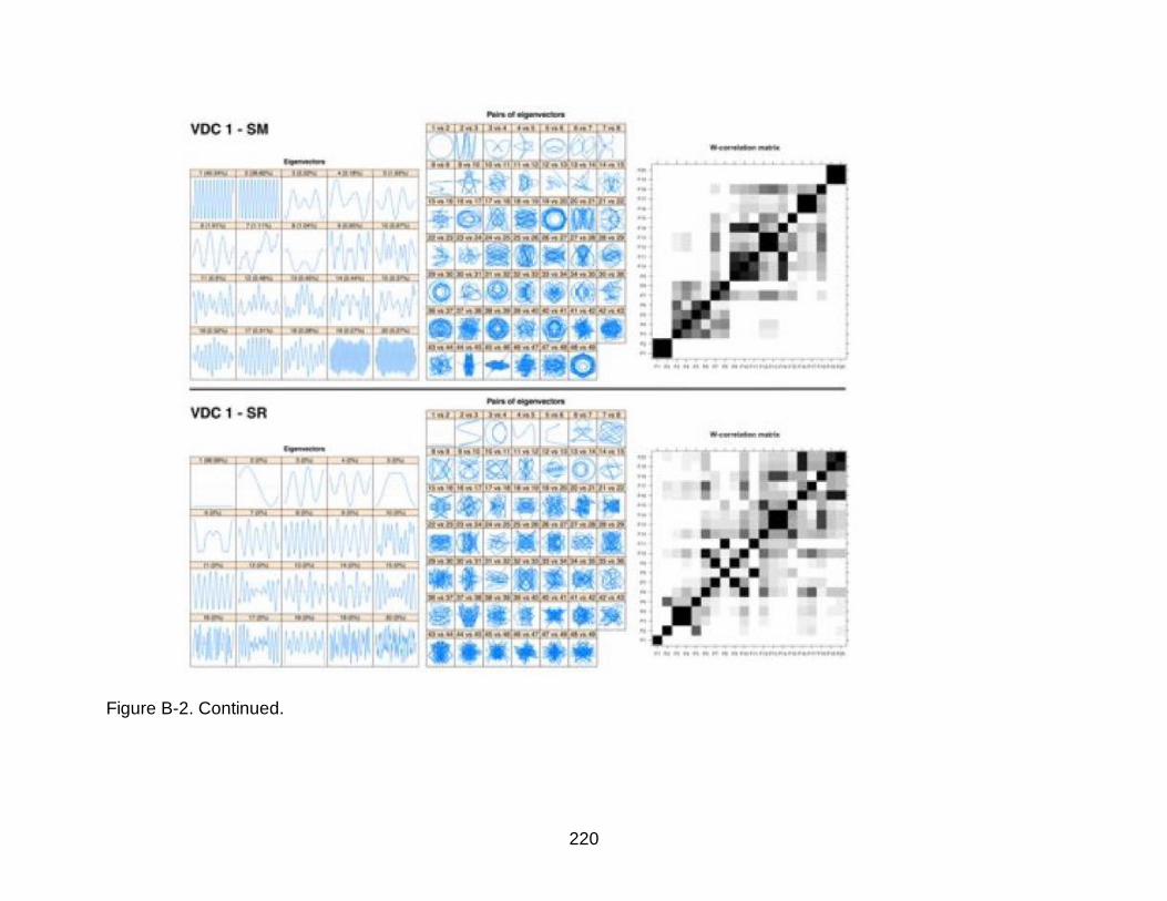
220
Figure B-2. Continued.

221
Figure B-3. Results of Singular Value Decomposition (VDC) of time series of VDC 2. From left to right: eigenvectors,
scatterplots of pairs of eigenvectors, and weighted correlation plots of pairs of eigenvectors.

222
Figure B-3. Continued.

223
Figure B-3. Continued.

224
Figure B-3. Continued.

225
Figure B-4. Results of Singular Value Decomposition (VDC) of time series of VDC 3. From left to right: eigenvectors,
scatterplots of pairs of eigenvectors, and weighted correlation plots of pairs of eigenvectors.

226
Figure B-4. Continued.

227
Figure B-4. Continued.

228
Figure B-4. Continued.

229
Figure B-5. Results of Singular Value Decomposition (VDC) of time series of VDC 4. From left to right: eigenvectors,
scatterplots of pairs of eigenvectors, and weighted correlation plots of pairs of eigenvectors.
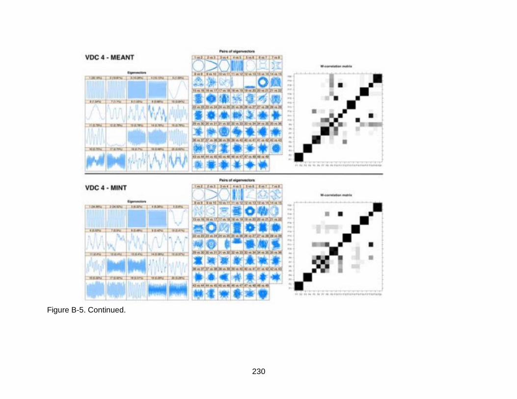
230
Figure B-5. Continued.

231
Figure B-5. Continued.

232
Figure B-5. Continued.

233
Figure B-6. Results of Singular Value Decomposition (VDC) of time series of climate indices. a) eigenvectors, b)
scatterplots of pairs of eigenvectors, and c) weighted correlation plots of pairs of eigenvectors.

234
Figure B-7. Lineplots and heatmaps of original and reconstructed time series of all variables for all 4 VDCs: maximum,
mean and minimum temperature, precipitation, potential evapotranspiration and soil moisture (A = VDC 1, B = VDC 2, C = VDC 3, D = VDC 4). In order: maximum temperature, mean temperature, minimum temperature, precipitation, potential evapotranspiration, soil moisture and climate indices. Climate variables (AMO, PDO, MEI) are not VDC related. First column is observed data, second column reconstructed. Months on the x-axis for the first two columns of plots.

235
Figure B-7. Continued.

236
Figure B-7. Continued.

237
Figure B-7. Continued.
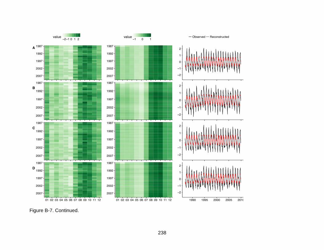
238
Figure B-7. Continued.
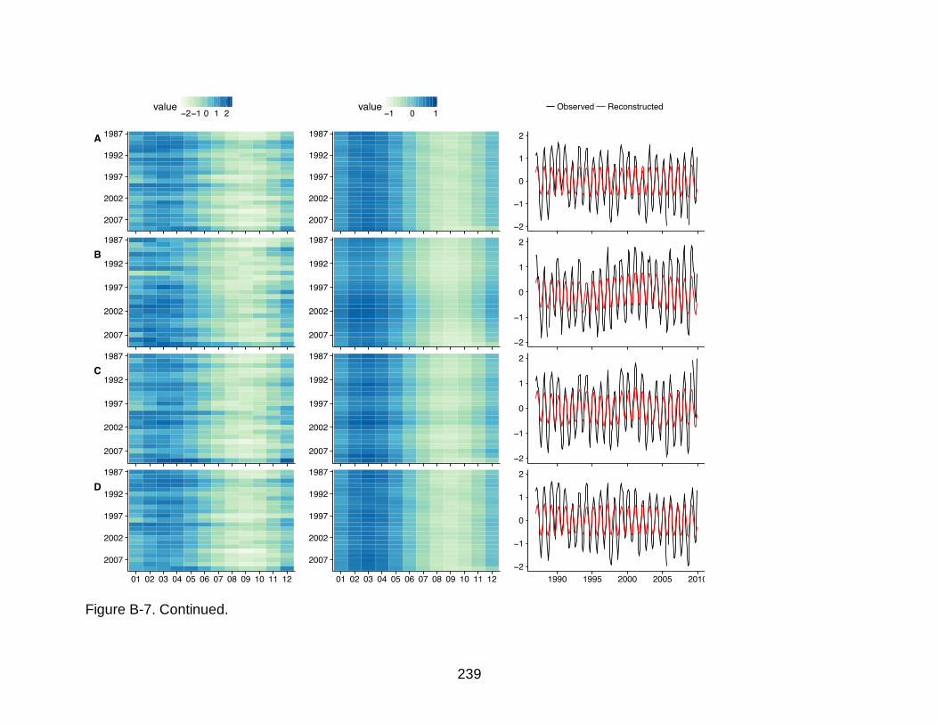
239
Figure B-7. Continued.

240
Figure B-7. Continued.

241
Figure B-8. Nonlinear cross-prediction skill to determine stationarity of signals, per VDC. Five segments are tested (black
lines), and an average is calculated across tests (red line).

242
Figure B-9. Networks of cross-mapping skill (𝜌) of deterministic signals (𝜌 ≥ 0.65) per VDC, after testing for false positives
due to synchronicity. Bidirectional causality between minimum, mean, maximum temperature, precipitation, potential evapotransporation and soil moisture are not shown. Species richness did not have a deterministic signal, so cross-mapping skill could not be determined. EVI = Enhanced Vegetation Index 2, MAXT = maximum temperature, MEANT = mean temperature, MINT = minimum temperature, P = precipitation, PET = potential evapotranspiration, SM = soil moisture, AMO = Atlantic Multidecadal Oscillation, PDO = Pacific Decadal Oscillation, MEI = Multivariate ENSO Index.

243
APPENDIX C ADDITIONAL NOTES ON GRANGER CAUSALITY ANALYSIS
Granger Prediction
CG analysis is more traditional causality analyses that we can apply to variables
(systems) that do not pass the tests for stationarity or (low-dimensional) determinism.
The basic tenet for GC is that if the prediction of a variable is improved by the inclusion
of another variable, this second variable is said to “Granger-cause” the first. Granger
formalized this with a series of linearized models (Granger, 1969). In order to remove
seasonality, which could bias the results to indicate causality due to strong
corresponding seasonality in two time series, we applied Multivariate Singular Spectrum
Analysis (MSSA). This method is similar to SSA, but it estimates signals that a number
of time series have in common and allows for signal reconstruction for each time series
separately. After removal of these shared seasonalities for each VDC, GC analysis was
applied to the remainders of each time series. For GC analysis, time series needed to
be stationary so any remaining trends over time needed to be removed. All time series
were evaluated for their order of integration with the KPSS-test and differentiated where
necessary. On the resulting time series, Vector Autoregression (VAR) was applied; it
captures linear interdependencies between multiple variables while also taking into
account the stochastic nature with the autoregressive components. The first VAR model
for Y consists of components with p-lagged vectors of the available variables (including
Y) and an error component:
𝑌𝑡 = ∑ 𝑎𝑖𝑌𝑡−𝑖𝑝𝑖−1 + ∑ 𝑏𝑖𝑋𝑡−𝑖
𝑝𝑖−1 + ∑ 𝑐𝑖𝑍𝑡−𝑖 + 휀1𝑡
𝑝𝑖−1 (C-1)
in which Y is the variable that is being tested for being driven by X, Z is the
collection of all other variables, a, b and c are coefficients (for c, a collection of

244
coefficients for each variable in Z), 휀 is the error component and p is the appropriate lag.
The latter was determined by first developing models for lags 1-12. The residuals were
checked for autocorrelation with the Ljung-Box test, and models with autocorrelated
residuals were discarded. Well-specified models should have residuals that are free of
autocorrelation. Next, the Aikaike Information Criterion (AIC) was calculated for the
remaining models, and out of these, the model with the lowest AIC was selected as the
best model. Next, using the same p, a second VAR model is developed without variable
X, the variable we want to test for Granger causing Y:
𝑌𝑡 = ∑ 𝑑𝑖𝑌𝑡−𝑖𝑝𝑖−1 + ∑ 𝑒𝑖𝑍𝑡−𝑖 + 휀2𝑡
𝑝𝑖−1 (C-2)
If the first model (with X) significantly improves the prediction of Y (i.e. the variance
contained in 휀1𝑡 is less than in 휀2𝑡), X is said to Granger cause Y. This is measured with
an F statistic:
𝐹 = ln(𝑅𝑆𝑆2 𝑅𝑆𝑆1⁄ ) (C-3)
with RSS the residual sum of squares for respectively VAR model 2 and VAR model 1.
If the presence of Z mediates any influence from X, bi will equal to zero, and the F
statistic will be zero since the error term has not changed. Conversely, less variance
contained in 휀1𝑡 generates a positive F statistic. The null hypothesis is that there is no
causality between variables, with 𝛼 = 0.05. Because of the presence of Z, this approach
is coined conditional Granger analysis, as opposed to ‘regular’ Granger analysis which
only considers X and Y. Other variables could (indirectly) affect this relationship, and by
taking into account this influence, otherwise misleading links are removed. Note that the
results of Granger analysis (or the VARs built) are not necessarily predictive tools, since
they do not evaluate goodness-of-fit specifically nor evaluate which covariates to

245
include or exclude. They give an indication of (potential) drivers of variables, which can
be used in the development of predictive models.
Results for Granger Prediction
GC analysis was applied to VDC 4 (see Chapter 3): since the EVI signal in VDC
4 violated the stationarity requirement (Chapter 5), this was the alternative causality
test. This way we could also test the CCM and GC results for agreement. The same
variables that were used in the CCM analysis were used in this test. Species richness
was also included in this analysis – it was excluded from the CCM analysis since no
signal was identified. Seasonality was removed from the VDC’s variables by applying
MSSA. Table C-1 and Figure C-1 summarizes the GC results. Tables C-2 and C-3
contain more details on the VAR models and full GC analysis. Take note that while p
values give a relative indication as to how much improvement a variable brings to
predicting another, GC analysis does not assign any strength to causal relationships.
This analysis shows a markedly different picture than CCM, with less dense causality
networks. Comparison with the previous analyses casts doubts on the completeness of
the causal networks and the results themselves. The GC analysis captures some of
causality that was also identified with CCM that we would continue to see, such as the
influence of EVI on minimum, maximum and mean temperature. Many causal
relationships that we expected to see are not identified with GC analysis, especially the
relationships between biophysical variables themselves (Table 5-3 and 5-4). There are
effects from variables onto the PDO, and from the MEI to a variable in GC analysis,
while CCM highlights the AMO as a central climate index. These variables do not differ
between VDCs, so results should be similar. Previous studies have found that GC
analysis misidentifies or misses causal relationships in comparison to CCM for known

246
systems (Lusch et al., 2016; Sugihara et al., 2012), and we conclude this is also the
case here. The only indication from this analysis is that the causality from EVI onto
maximum, mean and minimum temperature potentially increases. However, we deem
the results unsuitable as a representation of the complete causal network for the
system.
Discussion
In terms of methodology, as a result from these tests we would caution against using
GC analyses as a method to determine causality until there is a better understanding of
the conditions that affect performance of the analyses. Recent research has shown that
this method can give different results when inputs are only slightly changed, and that
accuracy varies with the density of the networks being estimated (Lusch et al., 2016).
For this study, where input data are either from reanalysis sources or remote sensing,
relying on GC would carry risk. We suspect that the EVI data are subject to
considerable noise due to the difficulty of measuring reflectance in the tropics during
times of high cloud cover and fires. The effect that this has on GC analysis is unknown.
While GC is spreading in popularity in environmental sciences (Damos, 2016; Detto et
al., 2012; B. Jiang et al., 2015; Kaufmann et al., 2003; 2004b; Notaro et al., 2006;
Papagiannopoulou et al., 2017; Tuttle and Salvucci, 2016), and many variations have
been developed on the original concept, it is not advised to use it as a tool to do causal
network mapping.

247
Table C-1. Results of Granger causality analysis for VDC 4. A variable Granger causes another variable if 𝑝 ≤ 0.05. The Nash-Sutcliffe Coefficient of Efficiency (NSE) indicates the goodness of fit of the full model (all variables included).
Variable Granger causes
Order of AR model
Ljung-Box p value
NSE of full model
F statistic
p value
EVI
MAXT 1 0.25 0.29
0.02 0.03
MEI 0.02 0.01 EVI
MEANT 1 0.36
0.31
0.12 0.00 MAXT 0.02 0.04 MEI 0.03 0.00 EVI MINT 10 0.16 0.76 0.20 0.00 MEI AMO 2 0.05 0.11 0.03 0.03 MAXT PDO 6 0.59 0.27 0.07 0.02

248
Table C-2. VAR models with p value for the Ljung-Box test > 0.05 Variable AR order AIC NSE Ljung-Box test: p
value
Cluster 1 EVI 2 -0.51 0.37 0.48 EVI 3 -0.50 0.39 0.25 EVI 4 -0.50 0.41 0.21 EVI 5 -0.50 0.44 0.73 EVI 6 -0.49 0.45 0.54 EVI 7 -0.49 0.48 0.60 EVI 8 -0.48 0.53 0.61 EVI 9 -0.48 0.57 0.10 EVI 10 -0.47 0.60 0.44 EVI 11 -0.47 0.67 0.43 EVI 12 -0.49 0.70 0.08 MAXT 1 -0.42 0.42 0.43 MAXT 2 -0.45 0.45 0.89 MAXT 3 -0.48 0.48 0.69 MAXT 4 -0.52 0.54 0.53 MAXT 5 -0.53 0.58 0.28 MAXT 6 -0.54 0.60 0.52 MAXT 7 -0.53 0.62 0.39 MAXT 8 -0.54 0.64 0.62 MAXT 9 -0.58 0.67 0.42 MAXT 10 -0.62 0.69 0.23 MAXT 11 -0.66 0.71 0.12 MAXT 12 -0.68 0.73 0.29 MEANT 1 -0.78 0.26 0.55 MEANT 2 -0.78 0.29 0.68 MEANT 3 -0.77 0.34 0.80 MEANT 4 -0.77 0.39 0.65 MEANT 5 -0.76 0.46 0.66 MEANT 6 -0.75 0.49 0.91 MEANT 7 -0.75 0.53 0.83 MEANT 8 -0.74 0.57 0.65 MEANT 9 -0.74 0.60 0.59 MEANT 10 -0.74 0.63 0.42 MEANT 11 -0.76 0.67 0.12 MEANT 12 -0.80 0.69 0.16 MINT 1 -1.33 0.44 0.11 MINT 2 -1.33 0.50 0.67 MINT 3 -1.35 0.52 0.61 MINT 4 -1.37 0.56 0.44 MINT 5 -1.41 0.60 0.72 MINT 6 -1.42 0.62 0.73 MINT 7 -1.46 0.67 0.78 MINT 8 -1.47 0.70 0.63 MINT 9 -1.46 0.72 0.59 MINT 10 -1.46 0.75 0.49 MINT 11 -1.51 0.77 0.15 MINT 12 -1.57 0.79 0.12 P 1 -0.77 0.25 0.41 P 2 -0.77 0.28 0.32 P 3 -0.77 0.32 0.85 P 4 -0.78 0.33 0.14
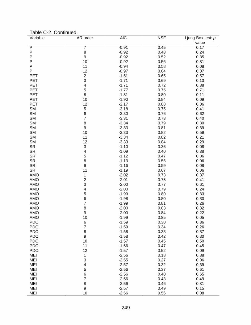
249
Table C-2. Continued. Variable AR order AIC NSE Ljung-Box test: p
value
P 7 -0.91 0.45 0.17 P 8 -0.92 0.48 0.24 P 9 -0.92 0.52 0.35 P 10 -0.92 0.56 0.31 P 11 -0.94 0.58 0.08 P 12 -0.97 0.64 0.07 PET 2 -1.51 0.65 0.57 PET 3 -1.71 0.69 0.13 PET 4 -1.71 0.72 0.38 PET 5 -1.77 0.75 0.71 PET 8 -1.81 0.80 0.11 PET 10 -1.90 0.84 0.09 PET 12 -2.17 0.88 0.06 SM 5 -3.18 0.75 0.41 SM 6 -3.30 0.76 0.62 SM 7 -3.31 0.78 0.40 SM 8 -3.34 0.79 0.30 SM 9 -3.33 0.81 0.39 SM 10 -3.33 0.82 0.59 SM 11 -3.34 0.82 0.21 SM 12 -3.33 0.84 0.29 SR 3 -1.10 0.36 0.08 SR 4 -1.09 0.40 0.38 SR 5 -1.12 0.47 0.06 SR 8 -1.13 0.56 0.06 SR 9 -1.16 0.59 0.08 SR 11 -1.19 0.67 0.06 AMO 1 -2.02 0.73 0.37 AMO 2 -2.01 0.75 0.41 AMO 3 -2.00 0.77 0.61 AMO 4 -2.00 0.79 0.24 AMO 5 -1.99 0.80 0.33 AMO 6 -1.98 0.80 0.30 AMO 7 -1.99 0.81 0.26 AMO 8 -2.00 0.83 0.32 AMO 9 -2.00 0.84 0.22 AMO 10 -1.99 0.85 0.05 PDO 6 -1.59 0.30 0.36 PDO 7 -1.59 0.34 0.26 PDO 8 -1.58 0.38 0.37 PDO 9 -1.58 0.42 0.30 PDO 10 -1.57 0.45 0.50 PDO 11 -1.56 0.47 0.45 PDO 12 -1.57 0.52 0.09 MEI 1 -2.56 0.18 0.38 MEI 3 -2.55 0.27 0.06 MEI 4 -2.57 0.32 0.39 MEI 5 -2.56 0.37 0.61 MEI 6 -2.56 0.40 0.65 MEI 7 -2.56 0.43 0.49 MEI 8 -2.56 0.46 0.31 MEI 9 -2.57 0.49 0.15 MEI 10 -2.56 0.56 0.08

250
Table C-2. Continued. Variable AR order AIC NSE Ljung-Box test: p
value
MEI 11 -2.56 0.59 0.09 MEI 12 -2.56 0.61 0.15 Cluster 2 EVI 10 -0.34 0.66 0.08 EVI 11 -0.36 0.69 0.12 EVI 12 -0.35 0.71 0.13 MAXT 1 -0.39 0.45 0.35 MAXT 3 -0.49 0.59 0.37 MAXT 4 -0.51 0.59 0.37 MAXT 5 -0.51 0.60 0.37 MAXT 6 -0.53 0.63 0.36 MAXT 7 -0.53 0.66 0.39 MAXT 8 -0.54 0.69 0.86 MAXT 9 -0.54 0.71 0.81 MAXT 10 -0.60 0.74 0.73 MAXT 11 -0.69 0.77 0.76 MAXT 12 -0.68 0.80 0.38 MEANT 1 -0.88 0.30 0.57 MEANT 2 -0.87 0.33 0.15 MEANT 3 -0.87 0.44 0.22 MEANT 4 -0.86 0.46 0.47 MEANT 5 -0.86 0.47 0.38 MEANT 6 -0.86 0.50 0.37 MEANT 7 -0.86 0.55 0.19 MEANT 8 -0.85 0.59 0.59 MEANT 9 -0.84 0.61 0.70 MEANT 10 -0.85 0.66 0.71 MEANT 11 -0.90 0.69 0.94 MEANT 12 -0.94 0.74 0.61 MINT 1 -1.31 0.44 0.05 MINT 2 -1.30 0.49 0.33 MINT 3 -1.33 0.56 0.22 MINT 4 -1.34 0.57 0.49 MINT 5 -1.38 0.59 0.28 MINT 6 -1.39 0.61 0.37 MINT 7 -1.39 0.65 0.19 MINT 8 -1.38 0.70 0.41 MINT 9 -1.40 0.71 0.55 MINT 10 -1.40 0.75 0.56 MINT 11 -1.47 0.77 0.92 MINT 12 -1.52 0.81 0.61 P 1 -0.77 0.29 0.19 P 2 -0.78 0.35 0.17 P 3 -0.80 0.41 0.30 P 4 -0.80 0.43 0.10 P 6 -0.90 0.51 0.17 P 7 -0.93 0.54 0.75 P 8 -0.93 0.56 0.83 P 9 -0.92 0.58 0.45 P 10 -0.92 0.64 0.68 P 11 -0.92 0.66 0.65 P 12 -0.91 0.68 0.60

251
Table C-2. Continued. Variable AR order AIC NSE Ljung-Box test: p
value
PET 3 -1.57 0.64 0.06 PET 5 -1.67 0.69 0.07 PET 7 -1.72 0.73 0.10 PET 8 -1.72 0.75 0.14 PET 9 -1.73 0.77 0.08 PET 10 -1.78 0.80 0.11 PET 11 -1.84 0.82 0.24 PET 12 -2.00 0.85 0.11 SM 4 -2.74 0.67 0.64 SM 5 -2.76 0.69 0.64 SM 6 -2.78 0.71 0.64 SM 7 -2.84 0.72 0.43 SM 9 -2.90 0.78 0.11 SM 10 -2.89 0.79 0.13 SM 11 -2.89 0.81 0.18 SR 3 -0.55 0.99 0.07 SR 4 -0.54 0.99 0.05 SR 5 -0.53 0.99 0.17 SR 12 -0.59 0.99 0.06 AMO 1 -2.02 0.73 0.34 AMO 2 -2.01 0.75 0.93 AMO 3 -2.00 0.76 0.55 AMO 6 -1.98 0.79 0.38 AMO 7 -1.99 0.79 0.44 AMO 8 -2.00 0.80 0.89 AMO 9 -2.00 0.81 0.53 AMO 10 -1.99 0.83 0.67 AMO 11 -1.98 0.85 0.51 AMO 12 -1.98 0.86 0.31 PDO 6 -1.59 0.30 0.34 PDO 7 -1.59 0.33 0.80 PDO 8 -1.58 0.35 0.76 PDO 9 -1.58 0.39 0.97 PDO 10 -1.57 0.44 0.15 PDO 11 -1.56 0.48 0.58 PDO 12 -1.57 0.51 0.27 MEI 1 -2.56 0.16 0.54 MEI 3 -2.55 0.27 0.10 MEI 4 -2.57 0.34 0.59 MEI 5 -2.56 0.39 0.87 MEI 6 -2.56 0.43 0.79 MEI 7 -2.56 0.44 0.68 MEI 8 -2.56 0.50 0.26 MEI 9 -2.57 0.52 0.06 MEI 10 -2.56 0.55 0.27 MEI 11 -2.56 0.59 0.19 MEI 12 -2.56 0.62 0.06 Cluster 3 EVI 2 -0.71 0.39 0.82 EVI 3 -0.71 0.40 0.68 EVI 4 -0.70 0.42 0.34 EVI 5 -0.70 0.47 0.34

252
Table C-2. Continued. Variable AR order AIC NSE Ljung-Box test: p
value
EVI 6 -0.69 0.50 0.16 EVI 10 -0.67 0.62 0.07 EVI 11 -0.67 0.65 0.05 MAXT 1 -0.72 0.23 0.89 MAXT 2 -0.71 0.29 0.72 MAXT 3 -0.71 0.35 0.34 MAXT 4 -0.71 0.37 0.59 MAXT 5 -0.70 0.40 0.61 MAXT 6 -0.70 0.43 0.69 MAXT 7 -0.69 0.46 0.56 MAXT 8 -0.69 0.53 0.38 MAXT 9 -0.68 0.56 0.28 MAXT 10 -0.68 0.59 0.10 MAXT 11 -0.70 0.61 0.19 MAXT 12 -0.72 0.65 0.11 MEANT 1 -0.61 0.42 0.25 MEANT 2 -0.65 0.48 0.93 MEANT 3 -0.66 0.51 0.59 MEANT 4 -0.67 0.53 0.87 MEANT 5 -0.68 0.56 0.89 MEANT 6 -0.68 0.59 0.77 MEANT 7 -0.69 0.62 0.61 MEANT 8 -0.72 0.65 0.28 MEANT 9 -0.77 0.67 0.32 MEANT 10 -0.85 0.69 0.13 MEANT 11 -0.88 0.71 0.28 MEANT 12 -0.89 0.74 0.11 MINT 1 -1.37 0.46 0.09 MINT 2 -1.36 0.54 0.60 MINT 3 -1.38 0.57 0.86 MINT 4 -1.42 0.59 0.51 MINT 5 -1.44 0.62 0.87 MINT 6 -1.45 0.65 0.89 MINT 7 -1.46 0.69 0.69 MINT 8 -1.45 0.71 0.12 MINT 9 -1.45 0.72 0.19 MINT 10 -1.48 0.75 0.08 MINT 11 -1.55 0.76 0.15 P 1 -0.83 0.23 0.40 P 2 -0.82 0.30 0.13 P 3 -0.83 0.34 0.44 P 4 -0.83 0.37 0.21 P 5 -0.87 0.45 0.17 P 6 -0.90 0.47 0.29 P 7 -0.92 0.49 0.24 P 8 -0.93 0.51 0.60 P 9 -0.93 0.56 0.39 P 10 -0.92 0.60 0.53 P 11 -0.93 0.62 0.82 P 12 -0.95 0.65 0.70 PET 3 -1.64 0.65 0.06 PET 4 -1.64 0.69 0.32 PET 5 -1.73 0.71 0.15

253
Table C-2. Continued. Variable AR order AIC NSE Ljung-Box test: p
value
PET 8 -1.76 0.79 0.27 PET 9 -1.76 0.82 0.40 PET 10 -1.86 0.84 0.54 PET 11 -1.93 0.85 0.65 PET 12 -2.19 0.88 0.10 SM 5 -3.14 0.93 0.33 SM 6 -3.13 0.94 0.21 SM 7 -3.16 0.94 0.06 SM 9 -3.18 0.95 0.14 SM 10 -3.18 0.95 0.16 SM 11 -3.18 0.96 0.41 SM 12 -3.17 0.96 0.36 SR 2 -1.01 0.59 0.07 SR 3 -1.01 0.60 0.20 SR 4 -1.03 0.62 0.22 SR 5 -1.03 0.64 0.45 SR 10 -1.08 0.76 0.13 AMO 1 -2.02 0.73 0.35 AMO 2 -2.01 0.75 0.82 AMO 3 -2.00 0.76 0.59 AMO 4 -2.00 0.77 0.22 AMO 5 -1.99 0.78 0.18 AMO 6 -1.98 0.78 0.14 AMO 7 -1.99 0.79 0.36 AMO 8 -2.00 0.80 0.95 AMO 9 -2.00 0.81 0.63 AMO 10 -1.99 0.82 0.21 AMO 12 -1.98 0.86 0.06 PDO 6 -1.58 0.30 0.38 PDO 7 -1.58 0.34 0.91 PDO 8 -1.57 0.37 0.86 PDO 9 -1.56 0.43 0.66 PDO 10 -1.56 0.45 0.27 PDO 11 -1.55 0.49 0.23 MEI 1 -2.56 0.17 0.28 MEI 4 -2.57 0.33 0.23 MEI 5 -2.56 0.37 0.41 MEI 6 -2.56 0.41 0.54 MEI 7 -2.56 0.43 0.69 MEI 8 -2.56 0.48 0.36 MEI 9 -2.57 0.52 0.14 MEI 10 -2.56 0.53 0.24 MEI 11 -2.56 0.58 0.34 MEI 12 -2.56 0.62 0.24 Cluster 4 EVI 2 -0.52 0.31 0.71 EVI 5 -0.54 0.46 0.22 EVI 6 -0.54 0.47 0.32 EVI 7 -0.53 0.50 0.23 EVI 8 -0.53 0.55 0.13 EVI 9 -0.52 0.58 0.10 EVI 10 -0.54 0.63 0.08

254
Table C-2. Continued. Variable AR order AIC NSE Ljung-Box test: p
value
MAXT 1 -0.46 0.45 0.96 MAXT 2 -0.52 0.47 0.67 MAXT 3 -0.54 0.49 0.94 MAXT 4 -0.56 0.52 0.19 MAXT 5 -0.57 0.56 0.13 MAXT 6 -0.58 0.57 0.09 MAXT 7 -0.57 0.62 0.08 MAXT 8 -0.60 0.65 0.55 MAXT 9 -0.63 0.67 0.49 MAXT 10 -0.68 0.70 0.21 MEANT 1 -0.79 0.22 0.80 MEANT 2 -0.78 0.25 0.65 MEANT 3 -0.78 0.30 0.94 MEANT 4 -0.77 0.32 0.09 MEANT 5 -0.76 0.40 0.12 MEANT 6 -0.76 0.44 0.08 MEANT 7 -0.75 0.52 0.05 MEANT 8 -0.75 0.56 0.58 MEANT 9 -0.74 0.58 0.37 MEANT 10 -0.74 0.61 0.12 MINT 1 -1.39 0.46 0.44 MINT 2 -1.38 0.49 0.80 MINT 3 -1.40 0.51 0.40 MINT 8 -1.49 0.71 0.36 MINT 9 -1.50 0.72 0.33 MINT 10 -1.53 0.74 0.08 P 9 -0.74 0.63 0.05 P 10 -0.78 0.65 0.16 PET 2 -1.43 0.60 0.14 PET 3 -1.60 0.64 0.17 PET 4 -1.60 0.67 0.86 PET 5 -1.67 0.69 0.69 PET 6 -1.67 0.72 0.13 PET 8 -1.70 0.76 0.22 PET 9 -1.69 0.80 0.52 PET 10 -1.80 0.82 0.65 PET 11 -1.84 0.83 0.28 PET 12 -2.14 0.86 0.12 SM 4 -3.22 0.76 0.26 SM 5 -3.23 0.78 0.55 SM 6 -3.37 0.79 0.82 SM 7 -3.38 0.80 0.37 SM 8 -3.43 0.82 0.56 SM 9 -3.42 0.82 0.67 SM 10 -3.42 0.83 0.43 SM 11 -3.44 0.85 0.38 SM 12 -3.44 0.87 0.34 SR 2 -1.92 0.67 0.27 SR 3 -1.93 0.69 0.47 SR 4 -1.92 0.70 0.10 SR 10 -1.94 0.81 0.11 SR 12 -1.98 0.84 0.16 AMO 1 -2.02 0.73 0.25

255
Table C-2. Continued. Variable AR order AIC NSE Ljung-Box test: p
value
AMO 2 -2.01 0.74 0.77 AMO 3 -2.00 0.75 0.52 AMO 4 -2.00 0.76 0.21 AMO 5 -1.99 0.78 0.16 AMO 6 -1.98 0.78 0.31 AMO 7 -1.99 0.78 0.59 AMO 8 -2.00 0.79 0.87 AMO 9 -2.00 0.80 0.95 AMO 10 -1.99 0.81 0.66 AMO 11 -1.98 0.82 0.40 AMO 12 -1.98 0.84 0.29 PDO 6 -1.59 0.37 0.61 PDO 7 -1.59 0.40 0.25 PDO 8 -1.58 0.43 0.51 PDO 9 -1.58 0.46 0.23 PDO 10 -1.57 0.50 0.22 PDO 11 -1.56 0.52 0.28 MEI 1 -2.56 0.19 0.38 MEI 4 -2.57 0.33 0.33 MEI 5 -2.56 0.37 0.56 MEI 6 -2.56 0.40 0.54 MEI 7 -2.56 0.44 0.71 MEI 8 -2.56 0.49 0.22 MEI 9 -2.57 0.51 0.23 MEI 10 -2.56 0.53 0.14 MEI 11 -2.56 0.57 0.13 MEI 12 -2.56 0.61 0.27

256
Table C-3. Granger causality test results for all variables (at selected AR order) Variable Granger causes AR order F statistic p value
Cluster 1 MAXT EVI 2 0.01 0.42 MEANT EVI 2 0.02 0.10 MINT EVI 2 0.03 0.03 P EVI 2 0.02 0.07 PET EVI 2 0.01 0.30 SM EVI 2 0.01 0.39 SR EVI 2 0.02 0.05 AMO EVI 2 0.02 0.07 PDO EVI 2 0.00 0.83 MEI EVI 2 0.02 0.14 EVI MAXT 12 0.04 0.93 MEANT MAXT 12 0.18 0.02 MINT MAXT 12 0.21 0.01 P MAXT 12 0.05 0.84 PET MAXT 12 0.07 0.67 SM MAXT 12 0.08 0.57 SR MAXT 12 0.09 0.39 AMO MAXT 12 0.06 0.82 PDO MAXT 12 0.08 0.50 MEI MAXT 12 0.07 0.72 EVI MEANT 12 0.05 0.83 MAXT MEANT 12 0.17 0.03 MINT MEANT 12 0.25 0.00 P MEANT 12 0.08 0.57 PET MEANT 12 0.11 0.27 SM MEANT 12 0.07 0.63 SR MEANT 12 0.09 0.42 AMO MEANT 12 0.07 0.72 PDO MEANT 12 0.09 0.41 MEI MEANT 12 0.07 0.67 EVI MINT 12 0.07 0.65 MAXT MINT 12 0.14 0.08 MEANT MINT 12 0.17 0.03 P MINT 12 0.10 0.37 PET MINT 12 0.17 0.02 SM MINT 12 0.06 0.77 SR MINT 12 0.09 0.47 AMO MINT 12 0.09 0.48 PDO MINT 12 0.12 0.20 MEI MINT 12 0.07 0.61 EVI P 12 0.06 0.75 MAXT P 12 0.12 0.18 MEANT P 12 0.08 0.51 MINT P 12 0.07 0.61 PET P 12 0.07 0.64 SM P 12 0.06 0.74 SR P 12 0.07 0.71 AMO P 12 0.13 0.14 PDO P 12 0.07 0.64 MEI P 12 0.06 0.73 EVI PET 12 0.04 0.93 MAXT PET 12 0.16 0.04

257
Table C-3. Continued. Variable Granger causes AR order F statistic p value
MEANT PET 12 0.17 0.03 MINT PET 12 0.17 0.03 P PET 12 0.04 0.95 SM PET 12 0.13 0.13 SR PET 12 0.11 0.23 AMO PET 12 0.05 0.89 PDO PET 12 0.08 0.54 MEI PET 12 0.06 0.82 EVI SM 8 0.04 0.45 MAXT SM 8 0.06 0.22 MEANT SM 8 0.07 0.13 MINT SM 8 0.08 0.05 P SM 8 0.04 0.57 PET SM 8 0.08 0.09 SR SM 8 0.06 0.25 AMO SM 8 0.05 0.29 PDO SM 8 0.03 0.71 MEI SM 8 0.04 0.52 EVI SR 11 0.11 0.13 MAXT SR 11 0.06 0.70 MEANT SR 11 0.06 0.69 MINT SR 11 0.03 0.93 P SR 11 0.13 0.06 PET SR 11 0.02 0.98 SM SR 11 0.12 0.08 AMO SR 11 0.10 0.18 PDO SR 11 0.06 0.62 MEI SR 11 0.05 0.80 EVI AMO 1 0.00 0.80 MAXT AMO 1 0.00 0.48 MEANT AMO 1 0.00 0.62 MINT AMO 1 0.00 0.57 P AMO 1 0.00 0.87 PET AMO 1 0.00 0.60 SM AMO 1 0.00 0.94 SR AMO 1 0.01 0.23 PDO AMO 1 0.00 0.89 MEI AMO 1 0.00 0.59 EVI PDO 6 0.01 0.97 MAXT PDO 6 0.02 0.62 MEANT PDO 6 0.01 0.93 MINT PDO 6 0.01 0.91 P PDO 6 0.01 0.98 PET PDO 6 0.04 0.31 SM PDO 6 0.02 0.66 SR PDO 6 0.04 0.21 AMO PDO 6 0.05 0.12 MEI PDO 6 0.02 0.80 EVI MEI 9 0.09 0.10 MAXT MEI 9 0.03 0.85 MEANT MEI 9 0.03 0.86 MINT MEI 9 0.04 0.58 P MEI 9 0.08 0.15 PET MEI 9 0.03 0.85

258
Table C-3. Continued. Variable Granger causes AR order F statistic p value
SM MEI 9 0.06 0.32 SR MEI 9 0.03 0.84 AMO MEI 9 0.03 0.80 PDO MEI 9 0.06 0.31 Cluster 2 MAXT EVI 11 0.06 0.60 MEANT EVI 11 0.11 0.16 MINT EVI 11 0.11 0.15 P EVI 11 0.13 0.06 PET EVI 11 0.10 0.23 SM EVI 11 0.10 0.21 SR EVI 11 0.06 0.65 AMO EVI 11 0.07 0.54 PDO EVI 11 0.04 0.86 MEI EVI 11 0.08 0.41 EVI MAXT 11 0.14 0.04 MEANT MAXT 11 0.21 0.00 MINT MAXT 11 0.19 0.00 P MAXT 11 0.03 0.95 PET MAXT 11 0.13 0.05 SM MAXT 11 0.07 0.46 SR MAXT 11 0.10 0.18 AMO MAXT 11 0.06 0.65 PDO MAXT 11 0.11 0.12 MEI MAXT 11 0.06 0.63 EVI MEANT 12 0.15 0.07 MAXT MEANT 12 0.23 0.00 MINT MEANT 12 0.25 0.00 P MEANT 12 0.03 0.98 PET MEANT 12 0.16 0.05 SM MEANT 12 0.14 0.09 SR MEANT 12 0.14 0.08 AMO MEANT 12 0.10 0.29 PDO MEANT 12 0.12 0.16 MEI MEANT 12 0.08 0.59 EVI MINT 12 0.13 0.14 MAXT MINT 12 0.21 0.00 MEANT MINT 12 0.23 0.00 P MINT 12 0.04 0.93 PET MINT 12 0.16 0.04 SM MINT 12 0.11 0.22 SR MINT 12 0.12 0.17 AMO MINT 12 0.12 0.18 PDO MINT 12 0.13 0.15 MEI MINT 12 0.07 0.62 EVI P 7 0.04 0.33 MAXT P 7 0.06 0.14 MEANT P 7 0.06 0.12 MINT P 7 0.06 0.09 PET P 7 0.03 0.55 SM P 7 0.05 0.26 SR P 7 0.12 0.00 AMO P 7 0.09 0.02

259
Table C-3. Continued. Variable Granger causes AR order F statistic p value
PDO P 7 0.05 0.21 MEI P 7 0.01 0.99 EVI PET 12 0.17 0.02 MAXT PET 12 0.14 0.09 MEANT PET 12 0.18 0.02 MINT PET 12 0.17 0.03 P PET 12 0.03 0.97 SM PET 12 0.11 0.25 SR PET 12 0.14 0.09 AMO PET 12 0.10 0.31 PDO PET 12 0.11 0.29 MEI PET 12 0.07 0.70 EVI SM 9 0.08 0.13 MAXT SM 9 0.03 0.83 MEANT SM 9 0.04 0.63 MINT SM 9 0.03 0.76 P SM 9 0.06 0.28 PET SM 9 0.08 0.16 SR SM 9 0.05 0.46 AMO SM 9 0.09 0.10 PDO SM 9 0.09 0.07 MEI SM 9 0.09 0.10 EVI SR 12 0.07 0.61 MAXT SR 12 0.09 0.44 MEANT SR 12 0.11 0.25 MINT SR 12 0.08 0.60 P SR 12 0.04 0.93 PET SR 12 0.11 0.26 SM SR 12 0.07 0.64 AMO SR 12 0.07 0.61 PDO SR 12 0.16 0.05 MEI SR 12 0.03 0.97 EVI AMO 1 0.00 0.81 MAXT AMO 1 0.00 0.91 MEANT AMO 1 0.00 0.34 MINT AMO 1 0.00 0.32 P AMO 1 0.00 0.73 PET AMO 1 0.00 0.29 SM AMO 1 0.00 0.87 SR AMO 1 0.00 0.53 PDO AMO 1 0.00 0.81 MEI AMO 1 0.00 0.55 EVI PDO 6 0.03 0.52 MAXT PDO 6 0.03 0.35 MEANT PDO 6 0.03 0.44 MINT PDO 6 0.02 0.53 P PDO 6 0.05 0.15 PET PDO 6 0.02 0.57 SM PDO 6 0.02 0.57 SR PDO 6 0.02 0.69 AMO PDO 6 0.08 0.01 MEI PDO 6 0.04 0.21 EVI MEI 9 0.03 0.88 MAXT MEI 9 0.05 0.49
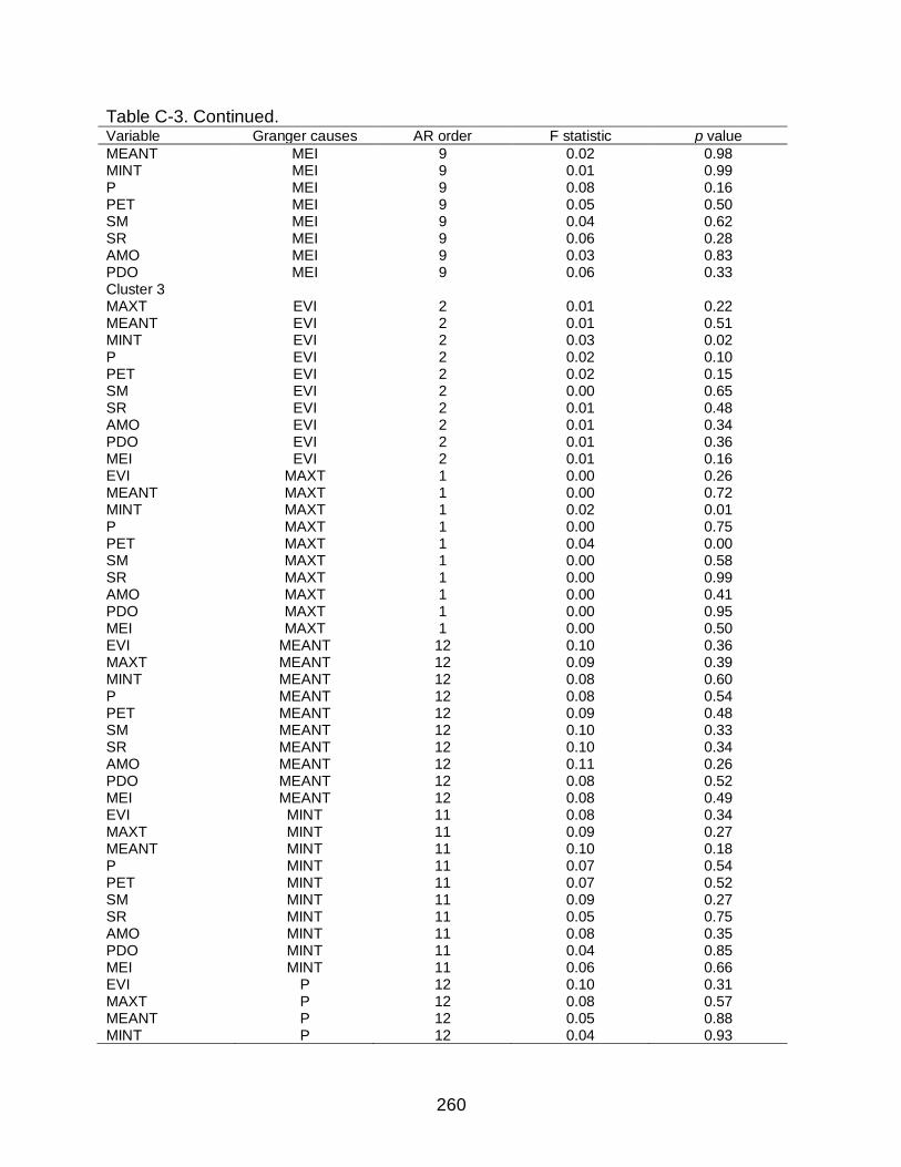
260
Table C-3. Continued. Variable Granger causes AR order F statistic p value
MEANT MEI 9 0.02 0.98 MINT MEI 9 0.01 0.99 P MEI 9 0.08 0.16 PET MEI 9 0.05 0.50 SM MEI 9 0.04 0.62 SR MEI 9 0.06 0.28 AMO MEI 9 0.03 0.83 PDO MEI 9 0.06 0.33 Cluster 3 MAXT EVI 2 0.01 0.22 MEANT EVI 2 0.01 0.51 MINT EVI 2 0.03 0.02 P EVI 2 0.02 0.10 PET EVI 2 0.02 0.15 SM EVI 2 0.00 0.65 SR EVI 2 0.01 0.48 AMO EVI 2 0.01 0.34 PDO EVI 2 0.01 0.36 MEI EVI 2 0.01 0.16 EVI MAXT 1 0.00 0.26 MEANT MAXT 1 0.00 0.72 MINT MAXT 1 0.02 0.01 P MAXT 1 0.00 0.75 PET MAXT 1 0.04 0.00 SM MAXT 1 0.00 0.58 SR MAXT 1 0.00 0.99 AMO MAXT 1 0.00 0.41 PDO MAXT 1 0.00 0.95 MEI MAXT 1 0.00 0.50 EVI MEANT 12 0.10 0.36 MAXT MEANT 12 0.09 0.39 MINT MEANT 12 0.08 0.60 P MEANT 12 0.08 0.54 PET MEANT 12 0.09 0.48 SM MEANT 12 0.10 0.33 SR MEANT 12 0.10 0.34 AMO MEANT 12 0.11 0.26 PDO MEANT 12 0.08 0.52 MEI MEANT 12 0.08 0.49 EVI MINT 11 0.08 0.34 MAXT MINT 11 0.09 0.27 MEANT MINT 11 0.10 0.18 P MINT 11 0.07 0.54 PET MINT 11 0.07 0.52 SM MINT 11 0.09 0.27 SR MINT 11 0.05 0.75 AMO MINT 11 0.08 0.35 PDO MINT 11 0.04 0.85 MEI MINT 11 0.06 0.66 EVI P 12 0.10 0.31 MAXT P 12 0.08 0.57 MEANT P 12 0.05 0.88 MINT P 12 0.04 0.93
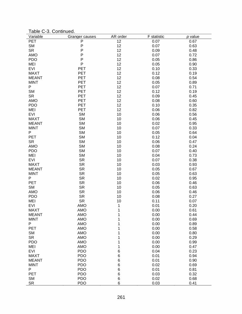
261
Table C-3. Continued. Variable Granger causes AR order F statistic p value
PET P 12 0.07 0.67 SM P 12 0.07 0.63 SR P 12 0.09 0.48 AMO P 12 0.07 0.72 PDO P 12 0.05 0.86 MEI P 12 0.05 0.90 EVI PET 12 0.10 0.33 MAXT PET 12 0.12 0.19 MEANT PET 12 0.08 0.54 MINT PET 12 0.05 0.89 P PET 12 0.07 0.71 SM PET 12 0.12 0.19 SR PET 12 0.09 0.45 AMO PET 12 0.08 0.60 PDO PET 12 0.10 0.35 MEI PET 12 0.06 0.82 EVI SM 10 0.06 0.56 MAXT SM 10 0.06 0.45 MEANT SM 10 0.02 0.95 MINT SM 10 0.07 0.33 P SM 10 0.05 0.64 PET SM 10 0.12 0.04 SR SM 10 0.06 0.47 AMO SM 10 0.08 0.24 PDO SM 10 0.07 0.40 MEI SM 10 0.04 0.73 EVI SR 10 0.07 0.38 MAXT SR 10 0.03 0.93 MEANT SR 10 0.05 0.67 MINT SR 10 0.05 0.63 P SR 10 0.02 0.95 PET SR 10 0.06 0.46 SM SR 10 0.05 0.63 AMO SR 10 0.06 0.46 PDO SR 10 0.08 0.27 MEI SR 10 0.11 0.07 EVI AMO 1 0.01 0.20 MAXT AMO 1 0.00 0.61 MEANT AMO 1 0.00 0.44 MINT AMO 1 0.00 0.69 P AMO 1 0.00 0.89 PET AMO 1 0.00 0.58 SM AMO 1 0.00 0.80 SR AMO 1 0.00 0.29 PDO AMO 1 0.00 0.99 MEI AMO 1 0.00 0.47 EVI PDO 6 0.04 0.23 MAXT PDO 6 0.01 0.94 MEANT PDO 6 0.01 0.90 MINT PDO 6 0.02 0.69 P PDO 6 0.01 0.81 PET PDO 6 0.03 0.32 SM PDO 6 0.02 0.68 SR PDO 6 0.03 0.41

262
Table C-3. Continued. Variable Granger causes AR order F statistic p value
AMO PDO 6 0.06 0.05 MEI PDO 6 0.03 0.49 EVI MEI 9 0.08 0.16 MAXT MEI 9 0.05 0.45 MEANT MEI 9 0.05 0.44 MINT MEI 9 0.04 0.59 P MEI 9 0.11 0.03 PET MEI 9 0.03 0.88 SM MEI 9 0.07 0.25 SR MEI 9 0.04 0.63 AMO MEI 9 0.04 0.62 PDO MEI 9 0.091 0.081 Cluster 4 MAXT EVI 6 0.03 0.40 MEANT EVI 6 0.03 0.32 MINT EVI 6 0.03 0.49 P EVI 6 0.05 0.09 PET EVI 6 0.06 0.06 SM EVI 6 0.02 0.61 SR EVI 6 0.02 0.68 AMO EVI 6 0.03 0.51 PDO EVI 6 0.01 0.81 MEI EVI 6 0.01 0.84 EVI MAXT 10 0.03 0.90 MEANT MAXT 10 0.14 0.02 MINT MAXT 10 0.14 0.01 P MAXT 10 0.05 0.66 PET MAXT 10 0.03 0.86 SM MAXT 10 0.09 0.17 SR MAXT 10 0.10 0.10 AMO MAXT 10 0.07 0.31 PDO MAXT 10 0.07 0.31 MEI MAXT 10 0.06 0.46 EVI MEANT 1 0.01 0.06 MAXT MEANT 1 0.00 0.63 MINT MEANT 1 0.01 0.24 P MEANT 1 0.00 0.76 PET MEANT 1 0.07 0.00 SM MEANT 1 0.02 0.01 SR MEANT 1 0.01 0.08 AMO MEANT 1 0.01 0.14 PDO MEANT 1 0.00 0.96 MEI MEANT 1 0.00 0.99 EVI MINT 10 0.04 0.83 MAXT MINT 10 0.06 0.51 MEANT MINT 10 0.12 0.05 P MINT 10 0.05 0.66 PET MINT 10 0.04 0.72 SM MINT 10 0.10 0.12 SR MINT 10 0.08 0.27 AMO MINT 10 0.11 0.07 PDO MINT 10 0.06 0.56 MEI MINT 10 0.06 0.52

263
Table C-3. Continued. Variable Granger causes AR order F statistic p value
EVI P 10 0.03 0.88 MAXT P 10 0.04 0.77 MEANT P 10 0.02 0.96 MINT P 10 0.01 1.00 PET P 10 0.05 0.58 SM P 10 0.05 0.63 SR P 10 0.05 0.57 AMO P 10 0.04 0.85 PDO P 10 0.11 0.06 MEI P 10 0.04 0.85 EVI PET 12 0.05 0.86 MAXT PET 12 0.07 0.72 MEANT PET 12 0.09 0.41 MINT PET 12 0.10 0.31 P PET 12 0.03 0.98 SM PET 12 0.08 0.54 SR PET 12 0.08 0.51 AMO PET 12 0.10 0.37 PDO PET 12 0.07 0.64 MEI PET 12 0.05 0.90 EVI SM 12 0.16 0.05 MAXT SM 12 0.15 0.07 MEANT SM 12 0.14 0.09 MINT SM 12 0.12 0.18 P SM 12 0.07 0.70 PET SM 12 0.17 0.03 SR SM 12 0.10 0.38 AMO SM 12 0.16 0.05 PDO SM 12 0.13 0.13 MEI SM 12 0.12 0.18 EVI SR 12 0.13 0.13 MAXT SR 12 0.08 0.57 MEANT SR 12 0.09 0.45 MINT SR 12 0.10 0.37 P SR 12 0.02 1.00 PET SR 12 0.06 0.81 SM SR 12 0.09 0.46 AMO SR 12 0.12 0.18 PDO SR 12 0.07 0.70 MEI SR 12 0.06 0.76 EVI AMO 1 0.01 0.19 MAXT AMO 1 0.00 0.70 MEANT AMO 1 0.00 0.78 MINT AMO 1 0.00 0.75 P AMO 1 0.00 0.56 PET AMO 1 0.00 0.90 SM AMO 1 0.00 0.35 SR AMO 1 0.00 0.88 PDO AMO 1 0.00 0.90 MEI AMO 1 0.00 0.53 EVI PDO 6 0.10 0.00 MAXT PDO 6 0.07 0.03 MEANT PDO 6 0.05 0.12 MINT PDO 6 0.03 0.47

264
Table C-3. Continued. Variable Granger causes AR order F statistic p value
P PDO 6 0.04 0.19 PET PDO 6 0.05 0.09 SM PDO 6 0.02 0.54 SR PDO 6 0.02 0.59 AMO PDO 6 0.06 0.06 MEI PDO 6 0.03 0.34 EVI MEI 9 0.09 0.11 MAXT MEI 9 0.06 0.40 MEANT MEI 9 0.05 0.47 MINT MEI 9 0.05 0.49 P MEI 9 0.02 0.91 PET MEI 9 0.06 0.33 SM MEI 9 0.05 0.43 SR MEI 9 0.05 0.51 AMO MEI 9 0.03 0.83 PDO MEI 9 0.09 0.07

265
Figure C-1. Conditional Granger causality (p<0.05) results for VDC 1 and VDC 4. a) Granger causality from other
variables onto EVI and climate indices for VDC 1, b) Granger causality from other variables onto EVI and climate indices for VDC 4, c) Granger causality from EVI and climate indices onto other variables for VDC 1, d) Granger causality from EVI and climate indoces onto other variables for VDC 4. Colors of the arrows indicate the range of the p-values. EVI = Enhanced Vegetation Index 2, MAXT = maximum temperature, MEANT = mean temperature, MINT = minimum temperature, P = precipitation, PET = potential evapotranspiration, SM = soil moisture, SR = species richness, AMO = Atlantic Multidecadal Oscillation, PDO = Pacific Decadal Oscillation, MEI = Multivariate ENSO Index.

266
LIST OF REFERENCES
Almeyda Zambrano, A., Broadbent, E., Schmink, M., Perz, S., Asner, G., 2010. Deforestation drivers in Southwest Amazonia: Comparing smallholder farmers in Iρapari, Peru, and Assis Brasil, Brazil. Conservat Soc 8, 157–14. doi:10.4103/0972-4923.73805
Andersen, T., Carstensen, J., Hernández-García, E., Duarte, C.M., 2009. Ecological
thresholds and regime shifts: approaches to identification. Trends in Ecology & Evolution 24, 49–57. doi:10.1016/j.tree.2008.07.014
Arias, P.A., Fu, R., Hoyos, C.D., Li, W., Zhou, L., 2010. Changes in cloudiness over the
Amazon rainforests during the last two decades: diagnostic and potential causes. Clim Dyn 37, 1151–1164. doi:10.1007/s00382-010-0903-2
Ashe, K., 2012. Elevated Mercury Concentrations in Humans of Madre de Dios, Peru.
PLoS ONE 7, e33305–6. doi:10.1371/journal.pone.0033305 Asner, G., Townsend, A.R., Braswell, B.H., 2000. Satellite observation of El Niño effects
on Amazon Forest phenology and productivity. Geophys. Res. Lett. 981–984. Baraloto, C., Alverga, P., Baéz Quispe, S., Barnes, G., Bejar Chura, N., Brasil da Silva,
I., Castro, W., da Souza, H., de Souza Moll, I., del Alcazar Chilo, J., Duenas Linares, H., Garate Quispe, J., Kenji, D., Medeiros, H., Murphy, S., Rockwell, C.A., Shenkin, A., Silveira, M., Southworth, J., Vasquez, G., Perz, S., 2014. Trade-offs among forest value components in community forests of southwestern Amazonia. E&S 19, art56–11. doi:10.5751/ES-06911-190456
Baraloto, C., Alverga, P., Quispe, S.B., Barnes, G., Chura, N.B., da Silva, I.B., Castro,
W., da Souza, H., de Souza Moll, I.E., del Alcazar Chilo, J., Linares, H.D., Quispe, J.G., Kenji, D., Marsik, M., Medeiros, H., Murphy, S., Rockwell, C., Selaya, G., Shenkin, A., Silveira, M., Southworth, J., Colomo, G.H.V., Perz, S., 2015. Effects of road infrastructure on forest value across a tri-national Amazonian frontier. Biol.Conserv. 191, 674–681. doi:10.1016/j.biocon.2015.08.024
Baraloto, C., Rabaud, S., Molto, Q., Blanc, L., Fortunel, C., Herault, B., Davila, N.,
Mesones, I., Rios, M., Valderrama, E., Fine, P.V.A., 2011. Disentangling stand and environmental correlates of aboveground biomass in Amazonian forests. Global Change Biol. 17, 2677–2688. doi:10.1111/j.1365-2486.2011.02432.x
Betts, R.A., Cox, P.M., Collins, M., Harris, P.P., Huntingford, C., Jones, C.D., 2004. The
role of ecosystem-atmosphere interactions in simulated Amazonian precipitation decrease and forest dieback under global climate warming. Theor Appl Climatol 78, 1–19. doi:10.1007/s00704-004-0050-y

267
Bosela, M., Popa, I., Gömöry, D., Longauer, R., Tobin, B., Kyncl, J., Kyncl, T., Nechita, C., Petráš, R., Sidor, C.G., Šebeň, V., Büntgen, U., 2016. Effects of post-glacial phylogeny and genetic diversity on the growth variability and climate sensitivity of European silver fir. J.Ecol. 104, 716–724. doi:10.1111/1365-2745.12561
BozorgMagham, A.E., Motesharrei, S., Penny, S.G., Kalnay, E., 2015. Causality
Analysis: Identifying the Leading Element in a Coupled Dynamical System. PLoS ONE 10, e0131226–17. doi:10.1371/journal.pone.0131226
Bradley, B.A., Fleishman, E., 2008. Can remote sensing of land cover improve species
distribution modelling? J.Biogeogr. 35, 1158–1159. doi:10.1111/j.1365-2699.2008.01928.x
Brajša, R., Wöhl, H., Hanslmeier, A., Verbanac, G., Ruždjak, D., Cliver, E., Svalgaard,
L., Roth, M., 2009. On solar cycle predictions and reconstructions. A&A 496, 855–861. doi:10.1051/0004-6361:200810862
Bressler, S.L., Seth, A.K., 2011. Wiener–Granger Causality: A well established
methodology. NeuroImage 58, 323–329. doi:10.1016/j.neuroimage.2010.02.059 Broadbent, E.N., Asner, G.P., Keller, M., Knapp, D.E., Oliveira, P.J., Silva, J.N., 2008.
Forest fragmentation and edge effects from deforestation and selective logging in the Brazilian Amazon. Biol.Conserv. 141, 1745–1757.
Brock, G., Datta, S., Pihur, V., Datt, S., 2008. clValid: An R Package for Cluster
Validation. Journal of Statistical Software 25, 1–22. Brown, K.A., Gurevitch, J., 2004. Long-term impacts of logging on forest diversity in
Madagascar. Proceedings of the National Academy of Sciences 101, 6045–6049. Cabello, J., Fernández, N., Alcaraz-Segura, D., Oyonarte, C., Piñeiro, G., Altesor, A.,
Delibes, M., Paruelo, J.M., 2012. The ecosystem functioning dimension in conservation: insights from remote sensing. Biodivers.Conserv. 21, 3287–3305. doi:10.1007/s10531-012-0370-7
Campo-Bescós, M.A., Muñoz-Carpena, R., Kaplan, D.A., Southworth, J., Zhu, L.,
Waylen, P.R., 2013. Beyond Precipitation: Physiographic Gradients Dictate the Relative Importance of Environmental Drivers on Savanna Vegetation. PLoS ONE 8, e72348–14. doi:10.1371/journal.pone.0072348
Carvalho, A.L. de, Nelson, B.W., Bianchini, M.C., Plagnol, D., Kuplich, T.M., Daly, D.C.,
2013. Bamboo-Dominated Forests of the Southwest Amazon: Detection, Spatial Extent, Life Cycle Length and Flowering Waves. PLoS ONE 8, e54852–13. doi:10.1371/journal.pone.0054852

268
Chambers, J.Q., Asner, G.P., Morton, D.C., Anderson, L.O., Saatchi, S.S., Espírito-Santo, F.D.B., Palace, M., Souza, C., Jr, 2007. Regional ecosystem structure and function: ecological insights from remote sensing of tropical forests. Trends in Ecology & Evolution 22, 414–423. doi:10.1016/j.tree.2007.05.001
Chazdon, R.L., 2003. Tropical forest recovery: legacies of human impact and natural
disturbances. Perspectives in Plant Ecology, Evolution and Systematics 6, 51–71. doi:10.1078/1433-8319-00042
Chen, J., Liu, Y., 2014. Coupled natural and human systems: a landscape ecology
perspective. Landscape Ecol. 46, 1139–4. doi:10.1007/s10980-014-0125-9 Chevan, A., Sutherland, M., 1991. Hierarchical Partitioning. The American Statistician
45, 90–96. Chouakria, A.D., Nagabhushan, P.N., 2007. Adaptive dissimilarity index for measuring
time series proximity. ADAC 1, 5–21. doi:10.1007/s11634-006-0004-6 Clark, A.T., Ye, H., Isbell, F., Deyle, E.R., Cowles, J., Tilman, G.D., Sugihara, G., 2015.
Spatial convergent cross mapping to detect causal relationships from short time series. Ecology 96, 1174–1181. doi:10.1890/14-1479.1
Coffin, A.W., 2007. From roadkill to road ecology: A review of the ecological effects of
roads 15, 396–406. doi:10.1016/j.jtrangeo.2006.11.006 Collins, D. and Phillips, T. 2011. Pacific-Atlantic route drives up fears of crime and
destruction. In: The Guardian (online). https://www.theguardian.com/environment/2011/jul/14/pacific-atlantic-route-brazil-peru Accessed: 3 October 2012
Collinson, C., Burnett, D., Agreda, V., 2000. Economic viability of Brazil nut trading in
Peru. Natural Resources Institute, University of Greenwich, Kent, UK. Convertino, M., Mangoubi, R.S., Linkov, I., Lowry, N.C., Desai, M., 2012. Inferring
Species Richness and Turnover by Statistical Multiresolution Texture Analysis of Satellite Imagery 7, e46616–16. doi:10.1371/journal.pone.0046616
Cumming, G.S., Barnes, G., Perz, S., Schmink, M., Sieving, K.E., Southworth, J.,
Binford, M., Holt, R.D., Stickler, C., Van Holt, T., 2005. An Exploratory Framework for the Empirical Measurement of Resilience. Ecosystems 8, 975–987. doi:10.1007/s10021-005-0129-z
Cumming, G.S., Southworth, J., Rondon, X.J., Marsik, M., 2012. Spatial complexity in
fragmenting Amazonian rainforests: Do feedbacks from edge effects push forests towards an ecological threshold? Ecological Complexity 11, 67–74.

269
D'Aleo, J., Easterbrook, D., 2010. Multidecadal Tendencies in ENSO and Global Temperatures Related to Multidecadal Oscillations. Energy & Environment 21, 437–460. doi:10.1260/0958-305X.21.5.437
Dakos, V., Bascompte, J., 2014. Critical slowing down as early warning for the onset of
collapse in mutualistic communities. Proc.Natl.Acad.Sci.U.S.A. 111, 17546–17551. doi:10.1073/pnas.1406326111
Dakos, V., Carpenter, S.R., Van Nes, E.H., Scheffer, M., 2014. Resilience indicators:
prospects and limitations for early warnings of regime shifts. Philosophical Transactions of the Royal Society B: Biological Sciences 370, 20130263–20130263. doi:10.1098/rstb.2013.0263
Dakos, V., Kéfi, S., Rietkerk, M., Van Nes, E.H., Scheffer, M., 2011. Slowing Down in
Spatially Patterned Ecosystems at the Brink of Collapse. Am.Nat. 177, E153–E166. doi:10.1086/659945
Dakos, V., Van Nes, E.H., D'Odorico, P., Scheffer, M., 2012. Robustness of variance
and autocorrelation as indicators of critical slowing down. Ecology 93, 264–271. Damos, P., 2016. Using multivariate cross correlations, Granger causality and graphical
models to quantify spatiotemporal synchronization and causality between pest populations. BMC Ecology 1–17. doi:10.1186/s12898-016-0087-7
Davidson, E.A., de Araújo, A.C., Artaxo, P., Balch, J.K., Brown, I.F., Bustamante,
M.M.C., Coe, M.T., DeFries, R.S., Keller, M., Longo, M., Munger, J.W., Schroeder, W., Soares-Filho, B.S., Souza, C.M., Wofsy, S.C., 2012. The Amazon basin in transition. Nature 481, 321–328. doi:10.1038/nature10717
Davis, R. E. Predictability of sea surface temperature and sea level pressure anomalies
over the North Pacific Ocean. Journal of Physical Oceanography 6, 249–266 (1976). De Groot, R.S., Wilson, M.A., Boumans, R.M., 2002. A typology for the classification,
description and valuation of ecosystem functions, goods and services. Ecol.Econ. 41, 393–408.
Detto, M., Molini, A., Katul, G., Stoy, P., Palmroth, S., Baldocchi, D., 2012. Causality
and Persistence in Ecological Systems: A Nonparametric Spectral Granger Causality Approach. Am.Nat. 179, 524–535. doi:10.1086/664628
DeWalt, S.J., Maliakal, S.K., Denslow, J.S., 2003. Changes in vegetation structure and
composition along a tropical forest chronosequence: implications for wildlife. For.Ecol.Manage. 182, 139–151. doi:10.1016/S0378-1127(03)00029-X
Dolan, K.T., Spano, M.L., 2001. Surrogate for nonlinear time series analysis. Phys. Rev.
E 64, 189–6. doi:10.1103/PhysRevE.64.046128

270
Donnelly, A., Yu, R., 2017. The rise of phenology with climate change: an evaluation of
IJB publications 1–22. doi:10.1007/s00484-017-1371-8 Douzal-Chouakria, A., Diallo, A., Giroud, F., 2009. Adaptive clustering for time series:
Application for identifying cell cycle expressed genes. Comput.Stat.Data Anal. 53, 1414–1426. doi:10.1016/j.csda.2008.11.031
Duchelle, A.E., Almeyda, A., Hoyos, N., Marsik, M., Broadbent, E., Kainer, A., 2010.
Conservation in an Amazon tri-national frontier: patterns and drivers of land cover change in community-managed forests, in:. Presented at the Taking stock of smallholder and community forestry where do we go from here, pp. 1–40.
Duchelle, A.E., Greenleaf, M., Mello, D., Gebara, M.F., Melo, T., 2014. Acre’s State
System of Incentives for Environmental Services (SISA), Brazil, in: Sills, E.O. (Ed.), REDD+ on the Ground. a Case Book of Subnational Initiatives Across the Globe. Center for International Forestry Research (CIFOR).
Dulac, J., 2013. Global Land Transport Infrastructure Requirements. International
Energy Agency. Dunn, J.C., 2008. Well-Separated Clusters and Optimal Fuzzy Partitions. Journal of
Cybernetics 4, 1–13. doi:10.1080/01969727408546059 Enfield, D.B., Mestas-Nuñez, A.M., Trimble, P.J., 2001. The Atlantic Multidecadal
Oscillation and its relation to rainfall and river flows in the continental U.S. Geophys. Res. Lett. 28, 2077–2080. doi:10.1029/2000GL012745
Fan, Y., 2004. Climate Prediction Center global monthly soil moisture data set at 0.5°
resolution for 1948 to present. J. Geophys. Res. 109, D10102–8. doi:10.1029/2003JD004345
Felton, A., Felton, A.M., Wood, J., Lindenmayer, D.B., 2006. Vegetation structure,
phenology, and regeneration in the natural and anthropogenic tree-fall gaps of a reduced-impact logged subtropical Bolivian forest. For.Ecol.Manage. 235, 186–193. doi:10.1016/j.foreco.2006.08.011
Findlay, C.S., Bourdages, J., 2000. Response Time of Wetland Biodiversity to Road
Construction on Adjacent Lands. Conserv.Biol. 14, 86–94. doi:10.1046/j.1523-1739.2000.99086.x
Fisher, J.I., Hurtt, G.C., Thomas, R.Q., Chambers, J.Q., 2008. Clustered disturbances
lead to bias in large-scale estimates based on forest sample plots. Ecol.Lett. 11, 554–563. doi:10.1111/j.1461-0248.2008.01169.x

271
Foley, J.A., Asner, G.P., Costa, M.H., Coe, M.T., DeFries, R.S., Gibbs, H.K., Howard, E.A., Olson, S., Patz, J., Ramankutty, N., Snyder, P., 2007. Amazonia revealed: forest degradation and loss of ecosystem goods and services in the Amazon Basin. Frontiers in Ecology and the Environment 5, 25–32.
Forman, R.T.T., 2003. Road ecology: science and solutions. Island Press. Frelich, L.E., Reich, P.B., 1999. Minireviews: Neighborhood Effects, Disturbance
Severity, and Community Stability in Forests. Ecosystems 2, 151–166. Gloor, M., Barichivich, J., Ziv, G., Brienen, R., Schöngart, J., Peylin, P., Ladvocat Cintra,
B.B., Feldpausch, T., Phillips, O., Baker, J., 2015. Recent Amazon climate as background for possible ongoing and future changes of Amazon humid forests. Global Biogeochem.Cycles 29, 1384–1399. doi:10.1002/2014GB005080
Golyandina, N., 2010. On the choice of parameters in singular spectrum analysis and
related subspace-based methods. Statistics and Its Interface 3, 259–279. doi:10.4310/SII.2010.v3.n3.a2
Golyandina, N., Shlemov, A., Korobeynikov, A., Usevich, K., 2014. Multivariate and 2D
extensions of Singular Spectrum Analysis with the Rssa package. arXiv. doi:arXiv:1309.5050
Golyandina, N., Zhigljavsky, A., 2013. Basic SSA, in: Singular Spectrum Analysis for
Time Series, SpringerBriefs in Statistics. Springer Berlin Heidelberg, Berlin, Heidelberg, pp. 11–70. doi:10.1007/978-3-642-34913-3_2
Granger, C.W.J., 1980. Testing for causality: a personal viewpoint. Journal of Economic
Dynamics and Control 2, 329–352. Granger, C.W.J., 1969. Investigating causal relations by econometric models and cross-
spectral methods. Econometrica 37, 424–438. Granger, C.W.J., 1963. Economic Processes Involving Feedback. Information and
Control 6, 28–48. Graves, S., Asner, G., Martin, R., Anderson, C., Colgan, M., Kalantari, L., Bohlman, S.,
2016. Tree Species Abundance Predictions in a Tropical Agricultural Landscape with a Supervised Classification Model and Imbalanced Data. Remote Sensing 8, 161–21. doi:10.3390/rs8020161
Grömping, U., 2006. Relative Importance for Linear Regression in R: The Package
relaimpo. Journal of Statistical Software 17, 1–27. doi:10.18637/jss.v017.i01

272
Guariguata, M.R., Ostertag, R., 2001. Neotropical secondary forest succession: changes in structural and functional characteristics. For.Ecol.Manage. 148, 185–206. doi:10.1016/S0378-1127(00)00535-1
Gunderson, L.H., Holling, C.S., 2002. Panarchy: understanding transformations in
systems of humans and nature. Island, Washington. Guo, S., Ladroue, C., Feng, J., 2010. Granger Causality: Theory and Applications, in:
Feng, J., Fu, W., Sun, F. (Eds.), Frontiers in Computational and Systems Biology. London, pp. 73–98. doi:https://doi.org/10.1007/978-1-84996-196-7_5
Guo, S., Seth, A.K., Kendrick, K.M., Zhou, C., Feng, J., 2008. Partial Granger
causality—Eliminating exogenous inputs and latent variables. Journal of Neuroscience Methods 172, 79–93. doi:10.1016/j.jneumeth.2008.04.011
Hannah, L., Carr, J.L., Lankerani, A., 1994. Human disturbance and natural habitat: a
biome level analysis of a global data set. Biodivers.Conserv. 4, 128–155. Hansen, B. E. Approximate asymptotic P values for structural-change tests. Journal of
Business and Economic Statistics 15, 60–67 (1997). Harris, I., Jones, P.D., Osborn, T.J., Lister, D.H., 2013. Updated high-resolution grids of
monthly climatic observations - the CRU TS3.10 Dataset. Int. J. Climatol. 34, 623–642. doi:10.1002/joc.3711
Hengl, T., de Jesus, J.M., MacMillan, R.A., Batjes, N.H., Heuvelink, G.B.M., Ribeiro, E.,
Samuel-Rosa, A., Kempen, B., Leenaars, J.G.B., Walsh, M.G., Gonzalez, M.R., 2014. SoilGrids1km — Global Soil Information Based on Automated Mapping. PLoS ONE 9, e105992–17. doi:10.1371/journal.pone.0105992
Herzog, S.K., Martinez, R., Jorgenson, P.M., Tiessen, H. (Eds.), 2011. Climate Change
and Biodiversity in the Tropical Andes. Inter-American Institute for Global Change (IAI) and Scientific Committee on Problems of the Environment (SCOPE).
Hirota, M., Holmgren, M., Van Nes, E.H., Scheffer, M., 2011. Global Resilience of
Tropical Forest and Savanna to Critical Transitions 334, 232–235. doi:10.1126/science.1210657
Hoelle, J., 2011. Convergence on Cattle: Political Ecology, Social Group Perceptions,
and Socioeconomic Relationships in Acre, Brazil. Culture, Agriculture, Food and Environment 33, 95–106. doi:10.1111/j.2153-9561.2011.01053.x
Holling, C.S., 1973. Resilience and Stability of Ecological Systems. Annu.Rev.Ecol.Syst.
4, 1–23.

273
Holmes, E.E., Ward, E.J., Scheuerell, M.D., 2014. Analysis of multivariate time- series using the MARSS package 1–262.
Huete, A., Didan, K., Miura, T., Rodriguez, E.P., Gao, X., Ferreira, L.G., 2002. Overview
of the radiometric and biophysical performance of the MODIS vegetation indices. Remote Sensing of Environment 83, 195–213.
Huete, A., Didan, K., van Leeuwen, W., Miura, T., Glenn, E., 2010. MODIS Vegetation
Indices, in: Ramachandran, B., Justice, C., Abrams, M. (Eds.), Land Remote Sensing and Global Environmental Change. Springer, New York, NY, pp. 579–602. doi:https://doi.org/10.1007/978-1-4419-6749-7_26
Huffaker, R., 2015. Building Economic Models Corresponding to the Real World. Appl.
Econ. Perspect. Pol. 37, 537–552. doi:10.1093/aepp/ppv021 Huffaker, R., Bittelli, M., Rosa, R., 2017. Nonlinear time series analysis with R. Oxford
University Press. Huffaker, R., Canavari, M., Muñoz-Carpena, R., 2016a. Distinguishing between
endogenous and exogenous price volatility in food security assessment: An empirical nonlinear dynamics approach. AGSY 1–12. doi:10.1016/j.agsy.2016.09.019
Huffaker, R., Muñoz-Carpena, R., Campo-Bescós, M.A., Southworth, J., 2016b.
Demonstrating correspondence between decision-support models and dynamics of real-world environmental systems. Environmental Modelling and Software 83, 74–87. doi:10.1016/j.envsoft.2016.04.024
Immitzer, M., Atzberger, C., Koukal, T., 2012. Tree Species Classification with Random
Forest Using Very High Spatial Resolution 8-Band WorldView-2 Satellite Data. Remote Sensing 4, 2661–2693. doi:10.3390/rs4092661
Jiang, B., Liang, S., Yuan, W., 2015. Observational evidence for impacts of vegetation
change on local surface climate over northern China using the Granger causality test. J. Geophys. Res. Biogeosci. 120, 1–12. doi:10.1002/2014JG002741
Jiang, Z., Huete, A., Didan, K., Miura, T., 2008. Development of a two-band enhanced
vegetation index without a blue band. Remote Sensing of Environment 112, 3833–3845. doi:10.1016/j.rse.2008.06.006
Johnson, J.W., Lebreton, J.M., 2004. History and Use of Relative Importance Indices in
Organizational Research. Organizational Research Methods 7, 238–257. doi:10.1177/1094428104266510
274
Kaplan, D., Muñoz-Carpena, R., 2011. Complementary effects of surface water and groundwater on soil moisture dynamics in a degraded coastal floodplain forest. Journal of Hydrology 398, 221–234.
Kaplan, D., Muñoz-Carpena, R., Ritter, A., 2010. Untangling complex shallow
groundwater dynamics in the floodplain wetlands of a southeastern U.S. coastal river. Water Resour.Res. 46, n/a–n/a. doi:10.1029/2009WR009038
Kaufmann, R.K., D'Arrigo, R.D., Laskowski, C., Myneni, R.B., Zhou, L., Davi, N.K.,
2004. The effect of growing season and summer greenness on northern forests. Geophys. Res. Lett. 31, n/a–n/a. doi:10.1029/2004GL019608
Kaufmann, R.K., Zhou, L., Myneni, R.B., Tucker, C.J., Slayback, D., Shabanov, N.V.,
Pinzon, J., 2003. The effect of vegetation on surface temperature: A statistical analysis of NDVI and climate data. Geophys. Res. Lett. 30, 449–4. doi:10.1029/2003GL018251
Keeling, H.C., Baker, T.R., Martinez, R.V., Monteagudo, A., Phillips, O.L., 2008.
Contrasting patterns of diameter and biomass increment across tree functional groups in Amazonian forests. Oecologia 158, 521–534. doi:10.1007/s00442-008-1161-4
Keller, M., 2009. Amazonia and global change. American Geophysical Union,
Washington, DC. Killeen, T.J., Solorzano, L.A., 2008. Conservation strategies to mitigate impacts from
climate change in Amazonia. Philosophical Transactions of the Royal Society B: Biological Sciences 363, 1881–1888. doi:10.1098/rstb.2007.0018
Klein, S.A., Soden, B.J., Lau, N.-C., 1999. Remote Sea Surface Temperature Variations
during ENSO: Evidence for a Tropical Atmospheric Bridge. J. Climate 12, 917–932. doi:10.1175/1520-0442(1999)012<0917:RSSTVD>2.0.CO;2
Koopmans, L.H., 1995. The spectral analysis of time series. Elsevier. doi:10.1016/B978-
012419251-5/50003-X Kuo, Y.-M., Lin, H.-J., 2010. Dynamic factor analysis of long-term growth trends of the
intertidal seagrass Thalassia hemprichii in southern Taiwan. Estuarine, Coastal and Shelf Science 86, 225–236. doi:10.1016/j.ecss.2009.11.017
Kuss, A.J.M., Gurdak, J.J., 2014. Groundwater level response in U.S. principal aquifers
to ENSO, NAO, PDO, and AMO. Journal of Hydrology 519, 1939–1952. doi:10.1016/j.jhydrol.2014.09.069

275
Laurance, W.F., Albernaz, A.K.M., Costa, C.D., 2002a. Is deforestation accelerating in the Brazilian Amazon? Environ.Conserv. 28, 1–7. doi:10.1017/S0376892901000339
Laurance, W.F., Clements, G.R., Sloan, S., O’Connell, C.S., Mueller, N.D., Goosem, M.,
Venter, O., Edwards, D.P., Phalan, B., Balmford, A., Van Der Ree, R., Arrea, I.B., 2014. A global strategy for road building. Nature 513, 229–232. doi:10.1038/nature13717
Laurance, W.F., Cochrane, M.A., Bergen, S., Fernside, P.M., Delamônica, P., Barber,
C., D'Angelo, S., Fernando, T., 2001. The Future of the Brazilian Amazon. Science 291, 438–439.
Laurance, W.F., Goosem, M., Laurance, S.G.W., 2009. Impacts of roads and linear
clearings on tropical forests. Trends in Ecology & Evolution 24, 659–669. doi:10.1016/j.tree.2009.06.009
Laurance, W.F., Lovejoy, T.E., Vasconcelos, H.L., Bruna, E.M., Didham, R.K., Stouffer,
P.C., Gascon, C., Bierregaard, R.O., Laurance, S.G., Sampaio, E., 2002b. Ecosystem decay of Amazonian forest fragments: a 22‐year investigation.
Conserv.Biol. 16, 605–618. Laurance, W.F., Schroth, G., Fearnside, P.M., Bergen, S., Venticinque, E.M., Da Costa,
C., 2002c. Predictors of Deforestation in the Brazilian Amazon. J.Biogeogr. 29, 737–748.
Laurance, W.F., Williamson, G.B., 2001. Positive feedbacks among forest
fragmentation, drought, and climate change in the Amazon. Conserv.Biol. 15, 1529–1535.
Lindeman, R.H., Merenda, P.F., Gold, R.Z., 1980. Introduction to bivariate and
multivariate analysis. Glenview, Ill: Scott, Foresman and Company. Liu, J., Dietz, T., Carpenter, S.R., Alberti, M., Folke, C., Moran, E., Pell, A.N., Deadman,
P., Kratz, T., Lubchenco, J., Ostrom, E., Ouyang, Z., Provencher, W., Redman, C.L., Schneider, S.H., Taylor, W.W., 2007. Complexity of coupled human and natural systems. Science 317, 1513–1516. doi:10.1126/science.1144004
Livina, V.N., Kwasniok, F., Lenton, T.M., 2010. Potential analysis reveals changing
number of climate states during the last 60 kyr. Climate of the Past 6, 77–82. doi:10.5194/cp-6-77-2010
Lugo, A.E., Gucinski, H., 2000. Function, effects, and management of forest roads.
For.Ecol.Manage. 133, 249–262.

276
Lusch, B., Maia, P.D., Kutz, J.N., 2016. Inferring connectivity in networked dynamical systems: Challenges using Granger causality. Phys. Rev. E 94, 125–14. doi:10.1103/PhysRevE.94.032220
Ma, H., Aihara, K., Chen, L., 2014. Detecting Causality from Nonlinear Dynamics with
Short-term Time Series. Nature Publishing Group 4, 7464–10. doi:10.1038/srep07464
Malhi, Y., Roberts, J.T., Betts, R.A., Killeen, T.J., Li, W., Nobre, C.A., 2008. Climate
Change, Deforestation, and the Fate of the Amazon. Science 319, 169–172. doi:10.1126/science.1146961
Mantua, N.J., Hare, S.R., Zhang, Y., Wallace, J.M., Francis, R.C., 1997. A Pacific
Interdecadal Climate Oscillation with Impacts on Salmon Production. Bull. Amer. Meteor. Soc. 78, 1069–1079. doi:10.1175/1520-0477(1997)078<1069:APICOW>2.0.CO;2
Marsik, M., Stevens, F.R., Southworth, J., 2011. Amazon deforestation: Rates and
patterns of land cover change and fragmentation in Pando, northern Bolivia, 1986 to 2005 35, 353–374. doi:10.1177/0309133311399492
Marthews, T.R., Quesada, C.A., Galbraith, D.R., Malhi, Y., Mullins, C.E., Hodnett, M.G.,
Dharssi, I., 2014. High-resolution hydraulic parameter maps for surface soils in tropical South America. Geosci. Model Dev. 7, 711–723. doi:10.5194/gmd-7-711-2014
Mendoza, E., Perz, S., Schmink, M., Nepstad, D., 2007. Participatory stakeholder
workshops to mitigate impacts of road paving in the Southwestern Amazon. Conservat Soc 5, 382–407.
Menzel, A., Sparks, T.H., Estrella, N., Koch, E., Aasa, A., Ahas, R., Alm-Kübler, K.,
Bissolli, P., Braslavska, O., Briede, A., Chmielewski, F.M., Crepinsek, Z., Curnel, Y., Dahl, Å., Defila, C., Donnelly, A., FILELLA, Y., Jatczak, K., Mage, F., Mestre, A., Nordli, Ø., Peñuelas, J., Pirinen, P., Remisova, V., Scheifinger, H., Striz, M., Susnik, A., van Vliet, A.J.H., Wielgolaski, F.-E., Zach, S., Zust, A., 2006. European phenological response to climate change matches the warming pattern. Global Change Biol. 12, 1969–1976. doi:10.1111/j.1365-2486.2006.01193.x
Mesquita, R.C.G., Delamônica, P., Laurance, W.F., 1999. Effect of surrounding
vegetation on edge-related tree mortality in Amazonian forest fragments. Biol.Conserv. 91, 129–134. doi:10.1016/S0006-3207(99)00086-5
Millennium Ecosystem Assessment, 2005. Ecosystems and human well-being. Island
Press Washington, DC.

277
Mitchell, T.P., Wallace, J.M., 1992. The annual cycle in equatorial convection and sea surface temperature. J. Climate 5, 1140–1156.
Morton, D.C., Nagol, J., Carabajal, C.C., Rosette, J., Palace, M., Cook, B.D., Vermote,
E.F., Harding, D.J., North, P.R.J., 2014. Amazon forests maintain consistent canopy structure and greenness during the dry season. Nature 506, 221–224. doi:10.1038/nature13006
Muñoz-Carpena, R., Ritter, A., Li, Y.C., 2005. Dynamic factor analysis of groundwater
quality trends in an agricultural area adjacent to Everglades National Park. J.Contam.Hydrol. 80, 49–70.
Myers, N., Mittermeier, R.A., Mittermeier, C.G., da Fonseca, G.A.B., Kent, J., 2000.
Biodiversity hotspots for conservation priorities. Nature 403, 853–858. Mønster, D., Fusaroli, R., Tylén, K., Roepstorff, A., Sherson, J.F., 2016. Inferring
Causality from Noisy Time Series Data - A Test of Convergent Cross-Mapping, in:. Presented at the 1st International Conference on Complex Information Systems, SCITEPRESS - Science and and Technology Publications, pp. 48–56. doi:10.5220/0005932600480056
Nash, J.E., Sutcliffe, J.V., 1970. River flow forecasting through conceptual models. Part
I - A discussion of principles. Journal of Hydrology 10, 282–290. Nepstad, D., Carvalho, G., Cristina Barros, A., Alencar, A., Paulo Capobianco, J.,
Bishop, J., Moutinho, P., Lefebvre, P., Lopes Silva, U., Jr., Prins, E., 2001. Road paving, fire regime feedbacks, and the future of Amazon forests. For.Ecol.Manage. 154, 395–407. doi:10.1016/S0378-1127(01)00511-4
Nepstad, D.C., Stickler, C.M., Soares- Filho, B., Merry, F., 2008. Interactions among
Amazon land use, forests and climate: prospects for a near-term forest tipping point. Philosophical transactions of the Royal Society of London.Series B, Biological sciences 363, 1737–1746.
Neter, J., Kutner, M.H., Nachtsheim, C.J., Wasserman, W., 1996. Applied linear
regression models. McGraw-Hill, Boston, Massachusetts, USA. Nobre, C.A., Borma, L.D.S., 2009. “Tipping points” for the Amazon forest.
Curr.Opin.Environ.Sustain. 1, 28–36. doi:10.1016/j.cosust.2009.07.003 Nogueira, E.M., Nelson, B.W., Fearnside, P.M., França, M.B., Oliveira, Á.C.A. de, 2008.
Tree height in Brazil's ‘arc of deforestation’: Shorter trees in south and southwest Amazonia imply lower biomass. For.Ecol.Manage. 255, 2963–2972. doi:10.1016/j.foreco.2008.02.002

278
Notaro, M., Liu, Z., Williams, J.W., 2006. Observed Vegetation–Climate Feedbacks in the United States*. J. Climate 19, 763–786. doi:10.1175/JCLI3657.1
OECD, 2011. Strategic Transport Infrastructure Needs to 2030. Offermann, D., Hoffmann, P., Knieling, P., Koppmann, R., Oberheide, J., Steinbrecht,
W., 2010. Long-term trends and solar cycle variations of mesospheric temperature and dynamics. J. Geophys. Res. 115, D18127–18. doi:10.1029/2009JD013363
Olivier, M.-D., Robert, S., Fournier, R.A., 2017. A method to quantify canopy changes
using multi-temporal terrestrial lidar data: Tree response to surrounding gaps. Agricultural and Forest Meteorology 237-238, 184–195. doi:10.1016/j.agrformet.2017.02.016
Ono, K., Punt, A.E., Hilborn, R., 2015. Think outside the grids: An objective approach to
define spatial strata for catch and effort analysis. Fisheries Research 170, 89–101. doi:10.1016/j.fishres.2015.05.021
Pachauri, R.K., Meyer, L., Plattner, G.K., Stocker, T., 2015. Climate Change 2014:
Synthesis Report. Contribution of Working Groups I, II and III to the Fifth Assessment Report of the Intergovernmental Panel on Climate Change. IPCC.
Palizdan, N., Falamarzi, Y., Huang, Y.F., Lee, T.S., 2016. Precipitation trend analysis
using discrete wavelet transform at the Langat River Basin, Selangor, Malaysia. Stochastic Environmental Research and Risk Assessment 31, 853–877. doi:10.1007/s00477-016-1261-3
Papagiannopoulou, C., Miralles, D.G., Decubber, S., Demuzere, M., Verhoest, N.E.C.,
Dorigo, W.A., Waegeman, W., 2017. A non-linear Granger-causality framework to investigate climate–vegetation dynamics. Geosci. Model Dev. 10, 1945–1960. doi:10.5194/gmd-10-1945-2017
Park, J., Dusek, G., 2013. ENSO components of the Atlantic multidecadal oscillation
and their relation to North Atlantic interannual coastal sea level anomalies. Ocean Sci. 9, 535–543. doi:10.5194/os-9-535-2013
Pereira, M.P.S., Malhado, A.C.M., Costa, M.H., 2012. Predicting land cover changes in
the Amazon rainforest: An ocean-atmosphere-biosphere problem. Geophys. Res. Lett. 39, n/a–n/a. doi:10.1029/2012GL051556
Peres, C.A., Baider, C., Zuidema, P.A., Wadt, L.H., Kainer, K.A., Gomes-Silva, D.A.,
Salomao, R.P., Simoes, L.L., Franciosi, E.R., Cornejo Valverde, F., Gribel, R., Shepard, G.H., Jr, Kanashiro, M., Coventry, P., Yu, D.W., Watkinson, A.R., Freckleton, R.P., 2003. Demographic threats to the sustainability of Brazil nut exploitation. Science 302, 2112–2114.

279
Perz, S., Brilhante, S., Brown, F., Caldas, M., Ikeda, S., Mendoza, E., Overdevest, C., Reis, V., Reyes, J.F., Rojas, D., Schmink, M., Souza, C., Walker, R., 2008. Road building, land use and climate change: prospects for environmental governance in the Amazon. Philosophical Transactions of the Royal Society B: Biological Sciences 363, 1889–1895. doi:10.1098/rstb.2007.0017
Perz, S.G., Cabrera, L., Carvalho, L.A., Castillo, J., Chacacanta, R., Cossio, R.E.,
Solano, Y.F., Hoelle, J., Perales, L.M., Puerta, I., Rojas Céspedes, D., Rojas Camacho, I., Costa Silva, A., 2011a. Regional integration and local change: road paving, community connectivity, and social–ecological resilience in a tri-national frontier, southwestern Amazonia. Regional Environmental Change 12, 35–53. doi:10.1007/s10113-011-0233-x
Perz, S.G., Muñoz-Carpena, R., Kiker, G., Holt, R.D., 2013a. Evaluating ecological
resilience with global sensitivity and uncertainty analysis. Ecol.Model. 263, 174–186. doi:10.1016/j.ecolmodel.2013.04.024
Perz, S.G., Overdevest, C., Caldas, M.M., Walker, R.T., Arima, E.Y., 2007. Unofficial
road building in the Brazilian Amazon: dilemmas and models for road governance. Environ.Conserv. 34, 112–121. doi:10.1017/s0376892907003827
Perz, S.G., Qiu, Y., Xia, Y., Southworth, J., Sun, J., Marsik, M., Rocha, K., Passos, V.,
Rojas, D., Alarcón, G., Barnes, G., Baraloto, C., 2013b. Trans-boundary infrastructure and land cover change: Highway paving and community-level deforestation in a tri-national frontier in the Amazon 34, 27–41. doi:10.1016/j.landusepol.2013.01.009
Perz, S.G., Rosero, M., Leite, F.L., Araujo Carvalho, L., Castillo, J., Vaca Mejia, C.,
2013c. Regional Integration and Household Resilience: Infrastructure Connectivity and Livelihood Diversity in the Southwestern Amazon. Hum Ecol 41, 497–511. doi:10.1007/s10745-013-9584-x
Perz, S.G., Shenkin, A., Barnes, G., Cabrera, L., Carvalho, L.A., Castillo, J., 2011b.
Connectivity and Resilience: A Multidimensional Analysis of Infrastructure Impacts in the Southwestern Amazon. Soc.Indicators Res. 106, 259–285. doi:10.1007/s11205-011-9802-0
280
Phillips, O.L., Aragão, L.E.O.C., Lewis, S.L., Fisher, J.B., Lloyd, J., López-González, G., Malhi, Y., Monteagudo, A., Peacock, J., Quesada, C.A., van der Heijden, G., Almeida, S., Amaral, I., Arroyo, L., Aymard, G., Baker, T.R., Bánki, O., Blanc, L., Bonal, D., Brando, P., Chave, J., de Oliveira, Á.C.A., Cardozo, N.D., Czimczik, C.I., Feldpausch, T.R., Freitas, M.A., Gloor, E., Higuchi, N., Jiménez, E., Lloyd, G., Meir, P., Mendoza, C., Morel, A., Neill, D.A., Nepstad, D., Patiño, S., Peñuela, M.C., Prieto, A., Ramírez, F., Schwarz, M., Silva, J., Silveira, M., Thomas, A.S., Steege, ter, H., Stropp, J., Vásquez, R., Zelazowski, P., Dávila, E.A., Andelman, S., Andrade, A., Chao, K.-J., Erwin, T., Di Fiore, A., C, E.H., Keeling, H., Killeen, T.J., Laurance, W.F., Cruz, A.P., Pitman, N.C.A., Vargas, P.N., Ramírez-Angulo, H., Rudas, A., Salamão, R., Silva, N., Terborgh, J., Torres-Lezama, A., 2009. Drought Sensitivity of the Amazon Rainforest. Science 323, 1344–1347. doi:10.1126/science.1164033
Phillips, O.L., Lewis, S.L., Baker, T.R., Chao, K.J., Higuchi, N., 2008. The changing
Amazon forest. Philosophical Transactions of the Royal Society B: Biological Sciences 363, 1819–1827. doi:10.1098/rstb.2007.0033
Phillips, O.L., Rose, S., Mendoza, A.M., Vargas, P.N., 2006. Resilience of Southwestern
Amazon Forests to Anthropogenic Edge Effects. Conserv.Biol. 20, 1698–1710. doi:10.1111/j.1523-1739.2006.00523.x
Phillips, O.L., Vargas, P.N., Monteagudo, A.L., Cruz, A.P., Zans, M.-E.C., Sanchez,
W.G., Yli-Halla, M., Rose, S., 2003. Habitat association among Amazonian tree species: a landscape-scale approach. J.Ecol. 91, 757–775. doi:10.1046/j.1365-2745.2003.00815.x
Pickett, S.T.A., Cadenasso, M.L., Grove, J.M., 2005. Biocomplexity in Coupled Natural–
Human Systems: A Multidimensional Framework. Ecosystems 8, 225–232. doi:10.1007/s10021-004-0098-7
Potter, C., Klooster, S., Huete, A., Genovese, V., Bustamante, M., Guimaraes Ferreira,
L., Cosme de Oliveira Junior, R., Zepp, R., 2009. Terrestrial carbon sinks in the Brazilian Amazon and Cerrado region predicted from MODIS satellite data and ecosystem modeling. Biogeosciences Discuss. 6, 947–969. doi:10.5194/bgd-6-947-2009
Putz, F.E., Redford, K.H., 2010. The importance of defining “forest”: tropical forest
degradation, deforestation, long‐term phase shifts, and further transitions. Biotropica
42, 10–20.

281
Quesada, C.A., Phillips, O.L., Schwarz, M., Czimczik, C.I., Baker, T.R., Patiño, S., Fyllas, N.M., Hodnett, M.G., Herrera, R., Almeida, S., Alvarez Dávila, E., Arneth, A., Arroyo, L., Chao, K.J., Dezzeo, N., Erwin, T., di Fiore, A., Higuchi, N., Honorio Coronado, E., Jimenez, E.M., Killeen, T., Lezama, A.T., Lloyd, G., López-González, G., Luizão, F.J., Malhi, Y., Monteagudo, A., Neill, D.A., Núñez Vargas, P., Paiva, R., Peacock, J., Peñuela, M.C., Peña Cruz, A., Pitman, N., Priante Filho, N., Prieto, A., Ramírez, H., Rudas, A., Salomão, R., Santos, A.J.B., Schmerler, J., Silva, N., Silveira, M., Vásquez, R., Vieira, I., Terborgh, J., Lloyd, J., 2012. Basin-wide variations in Amazon forest structure and function are mediated by both soils and climate. Biogeosciences 9, 2203–2246. doi:10.5194/bg-9-2203-2012
Ramanuja Rao, K., 1973. Short periodicities in solar activity. Solar Physics 29, 47–53. Rapp, K., 2005. The Brazil-Peru Trans Oceanic Highway. Project Summary. Redwood, J., 2012. The Environmental and Social Impacts of Major IDB-Financed Road
Improvement Projects: The Interoceanica IIRSA Sur and IIRSA Norte Highways in Peru. Inter-American Development Bank.
Reed, B.C., Brown, J.F., VanderZee, D., Loveland, T., Merchant, J.W., Ohlen, D.O.,
1994. Measuring phenological variability from satellite imagery. Journal of Vegetation Science 5, 703–714.
Restrepo-Coupe, N., da Rocha, H.R., Hutyra, L.R., da Araujo, A.C., Borma, L.S.,
Christoffersen, B., Cabral, O.M.R., de Camargo, P.B., Cardoso, F.L., da Costa, A.C.L., Fitzjarrald, D.R., Goulden, M.L., Kruijt, B., Maia, J.M.F., Malhi, Y.S., Manzi, A.O., Miller, S.D., Nobre, A.D., Randow, von, C., Sá, L.D.A., Sakai, R.K., Tota, J., Wofsy, S.C., Zanchi, F.B., Saleska, S.R., 2013. What drives the seasonality of photosynthesis across the Amazon basin? A cross-site analysis of eddy flux tower measurements from the Brasil flux network. Agricultural and Forest Meteorology 182-183, 128–144. doi:10.1016/j.agrformet.2013.04.031
Ritter, A., Muñoz-Carpena, R., 2013. Performance evaluation of hydrological models:
Statistical significance for reducing subjectivity in goodness-of-fit assessments. Journal of Hydrology 480, 33–45. doi:10.1016/j.jhydrol.2012.12.004
Roberts. 2011. Interoceanic Highway - Road to Ruin? In The Argentina Independent (online). http://www.argentinaindependent.com/currentaffairs/latest-news/newsfromargentina/interoceanic-highway-road-to-ruin/ Accessed 11 September 2012
282
Rockwell, C.A., Guariguata, M.R., Menton, M., Arroyo Quispe, E., Quaedvlieg, J., Warren-Thomas, E., Fernandez Silva, H., Jurado Rojas, E.E., Kohagura Arrunátegui, J.A.H., Meza Vega, L.A., Revilla Vera, O., Quenta Hancco, R., Valera Tito, J.F., Villarroel Panduro, B.T., Yucra Salas, J.J., 2015. Nut Production in Bertholletia excelsa across a Logged Forest Mosaic: Implications for Multiple Forest Use. PLoS ONE 10, e0135464–22. doi:10.1371/journal.pone.0135464
Rockwell, C.A., Kainer, K.A., d’Oliveira, M.V.N., Staudhammer, C.L., Baraloto, C., 2014.
Logging in bamboo-dominated forests in southwestern Amazonia: Caveats and opportunities for smallholder forest management. For.Ecol.Manage. 315, 202–210. doi:10.1016/j.foreco.2013.12.022
Rousseeuw, P.J., 1987. Silhouettes: a graphical aid to the interpretation and validation
of cluster analysis. Journal of Computational and Applied Mathematics 20, 53–65. Roy, Sen, S., 2010. Identification of periodicity in the relationship between PDO, El Niño
and peak monsoon rainfall in India using S-transform analysis. Int. J. Climatol. 31, 1507–1517. doi:10.1002/joc.2172
Running, S.W., Nemani, R., Glassy, J.M., Thornton, P.E., 1999. MODIS Daily
Photosynthesis (PSN) and Annual Net Primary Production (NPP) Product (MOD17). Rybansky, M., Brenova, M., Cermak, J., van Genderen, J., Sivertun, Å., 2016.
Vegetation structure determination using LIDAR data and the forest growth parameters. IOP Conf. Ser.: Earth Environ. Sci. 37, 012031–8. doi:10.1088/1755-1315/37/1/012031
Salimon, C.I., Putz, F.E., Menezes-Filho, L., Anderson, A., Silveira, M., Brown, I.F.,
Oliveira, L.C., 2011. Estimating state-wide biomass carbon stocks for a REDD plan in Acre, Brazil. For.Ecol.Manage. 262, 555–560. doi:10.1016/j.foreco.2011.04.025
Sanderson, E.W., Jaiteh, M., Levy, M.A., Redford, K.H., Wannebo, A.V., Woolmer, G.,
2002. The Human Footprint and the Last of the Wild. BioScience 52, 891–14. doi:10.1641/0006-3568(2002)052[0891:THFATL]2.0.CO;2
Santos, dos, A.J., Vieira, T.B., de Cassia Faria, K., 2016. Effects of vegetation structure
on the diversity of bats in remnants of Brazilian Cerrado savanna. Basic and Applied Ecology 17, 720–730. doi:10.1016/j.baae.2016.09.004
Sasaki, N., Putz, F.E., 2009. Critical need for new definitions of “forest” and ‘forest
degradation’ in global climate change agreements. Conservation Letters 2, 226–232.
Scheffer, M., 2009. Critical transitions in nature and society. Princeton University Press.

283
Scheffer, M., Bascompte, J., Brock, W.A., Brovkin, V., Carpenter, S.R., Dakos, V., Held, H., Van Nes, E.H., Rietkerk, M., Sugihara, G., 2009. Early-warning signals for critical transitions 461, 53–59. doi:10.1038/nature08227
Scheffer, M., Carpenter, S., Foley, J.A., Folke, C., Walker, B., 2001. Catastrophic shifts
in ecosystems. Nature 413, 591–596. Scullion, J.J., Vogt, K.A., Sienkiewicz, A., Gmur, S.J., Trujillo, C., 2014. Assessing the
influence of land-cover change and conflicting land-use authorizations on ecosystem conversion on the forest frontier of Madre de Dios, Peru. Biol.Conserv. 171, 247–258. doi:10.1016/j.biocon.2014.01.036
Silva, F.B., Shimabukuro, Y.E., Aragão, L.E.O.C., Anderson, L.O., Pereira, G., Cardozo,
F., Arai, E., 2013. Large-scale heterogeneity of Amazonian phenology revealed from 26-year long AVHRR/NDVI time-series. Environ. Res. Lett. 8, 024011–15. doi:10.1088/1748-9326/8/2/024011
Silva, G.A.M.D., Drumond, A., Ambrizzi, T., 2011. The impact of El Niño on South
American summer climate during different phases of the Pacific Decadal Oscillation. Theor Appl Climatol 106, 307–319. doi:10.1007/s00704-011-0427-7
Small, M., Tse, C.K., 2003. Detecting determinism in time series: The method of
surrogate data. Circuits and Systems I: Fundamental Theory and Applications, IEEE Transactions on 50, 663–672.
Small, M., Tse, C.K., 2002. Applying the method of surrogate data to cyclic time series.
Physica D 164, 187–201. doi:10.1016/S0167-2789(02)00382-2 Sousa, W.P., 1984. The role of disturbance in natural communities.
Annu.Rev.Ecol.Syst. 15, 353–391. Southworth, J., Marsik, M., Qiu, Y., Perz, S., Cumming, G., Stevens, F., Rocha, K.,
Duchelle, A., Barnes, G., 2011. Roads as Drivers of Change: Trajectories across the
Tri‑National Frontier in MAP, the Southwestern Amazon. Remote Sensing 3, 1047–
1066. doi:10.3390/rs3051047 Stockholm Resilience Centre. 2012. What is resilience?
http://www.stockholmresilience.org/21/research/what-is-resilience/research-background/research-framework/social-ecological-systems.html Accessed 13 December 2012.
Sugihara, G., May, R., Ye, H., Hsieh, C.H., Deyle, E., Fogarty, M., Munch, S., 2012.
Detecting Causality in Complex Ecosystems. Science 338, 496–500. doi:10.1126/science.1227079
Theiler, J., Eubank, S., A, A.L., Galdrikian, B., Farmer, J., 1992. Testing for nonlinearity

284
in time series: the method of surrogate data. Physica D 58, 77–94. Thonicke, K., Venevsky, S., Sitch, S., Kramer, W., 2001. The role of fire disturbance for
global vegetation dynamics: coupling fire into a Dynamic Global Vegetation Model. Global Ecol.Biogeogr. 10, 661–677.
Tilman, D., 2001. Functional diversity. Encyclopedia of biodiversity 3, 109–120. Tuttle, S., Salvucci, G., 2016. Empirical evidence of contrasting soil moisture-
precipitation feedbacks across the United States. Science 352, 825–827. doi:10.1126/science.aaa7185
Van Nes, E.H., Scheffer, M., Brovkin, V., Lenton, T.M., Ye, H., Deyle, E., Sugihara, G.,
2015. Causal feedbacks in climate change. Nature Climate change 5, 445–448. doi:10.1038/nclimate2568
Velasco, E.M., Gurdak, J.J., Dickinson, J.E., Ferré, T.P.A., Corona, C.R., 2017.
Interannual to multidecadal climate forcings on groundwater resources of the U.S. West Coast. Biochemical Pharmacology 11, 250–265. doi:10.1016/j.ejrh.2015.11.018
Verbesselt, J., Umlauf, N., Hirota, M., Holmgren, M., Van Nes, E.H., Herold, M., Zeileis,
A., Scheffer, M., 2016. Remotely sensed resilience of tropical forests. Nature Climate change 6, 1028–1031. doi:10.1038/nclimate3108
Verrelst, J., Camps-Valls, G., Muñoz-Marí, J., Rivera, J.P., Veroustraete, F., Clevers,
J.G.P.W., Moreno, J., 2015. Optical remote sensing and the retrieval of terrestrial vegetation bio-geophysical properties – A review. ISPRS Journal of Photogrammetry and Remote Sensing 108, 273–290. doi:10.1016/j.isprsjprs.2015.05.005
Volante, J.N., Alcaraz-Segura, D., Mosciaro, M.J., Viglizzo, E.F., Paruelo, J.M., 2012.
Ecosystem functional changes associated with land clearing in NW Argentina. “Agriculture, Ecosystems and Environment” 154, 12–22. doi:10.1016/j.agee.2011.08.012
Walker, W., Baccini, A., Schwartzmann, S., Ríos, S., Oliveira-Miranda, M.A., Augusto,
C., Ruiz, M.R., Arrasco, C.S., Ricardo, B., Smith, R., Meyer, C., Jintiach, J.C., Campos, E.V., 2014. Forest carbon in Amazonia: the unrecognized contribution of indigenous territories and protected natural areas. Carbon Management. doi:10.1080/17583004.2014.990680
Wang, J., Yang, B., Ljungqvist, F.C., Zhao, Y., 2013. The relationship between the
Atlantic Multidecadal Oscillation and temperature variability in China during the last millennium. J. Quaternary Sci. 28, 653–658. doi:10.1002/jqs.2658

285
Weinhold, D., Reis, E.J., 2001. Model evaluation and causality testing in short panels: the case of infrastructure provision and population growth in the Brazilian Amazon. Journal of Regional Science 41, 639–658.
Weng, Q., 2011. Advances in environmental remote sensing: sensors, algorithms, and
applications. CRC Press. Wissel, C., 1984. A universal law of the characteristic return time near thresholds.
Oecologia 65, 101–107. Wolf, A.A., Zavaleta, E.S., Selmants, P.C., 2017. Flowering phenology shifts in
response to biodiversity loss. Proc.Natl.Acad.Sci.U.S.A. 114, 3463–3468. doi:10.1073/pnas.1608357114
Wolter, K., Timlin, M.S., 2012. Measuring the strength of ENSO events: How does
1997/98 rank? Weather 53, 315–324. Ye, H., Deyle, E.R., Gilarranz, L.J., Sugihara, G., 2015. Distinguishing time-delayed
causal interactions using convergent cross mapping. Nature Publishing Group 5, 1–9. doi:10.1038/srep14750
Zeeman, E.C., 1976. Catastrophe Theory. Scientific American 234, 65–83. Zeileis, A., Kleiber, C., Krämer, W., Hornik, K., 2003. Testing and dating of structural
changes in practice. Comput.Stat.Data Anal. 44, 109–123. doi:10.1016/S0167-9473(03)00030-6
Zeileis, A., Leisch, F., Hornik, K., Kleiber, C., 2002. strucchange: An RPackage for
Testing for Structural Change in Linear Regression Models. Journal of Statistical Software 7, 1–38. doi:10.18637/jss.v007.i02
Zhang, Y., Wallace, J.M., Battisti, D.S., 1997. ENSO-like Interdecadal Variability: 1900–
93. J. Climate 10, 1004–1020. doi:10.1175/1520-0442(1997)010<1004:ELIV>2.0.CO;2
Zhou, Z., Chen, Y., Ding, M., Wright, P., Lu, Z., Liu, Y., 2009. Analyzing brain networks
with PCA and conditional Granger causality. Hum. Brain Mapp. 30, 2197–2206. doi:10.1002/hbm.20661
Zhu, J., Mao, Z., Hu, L., Zhang, J., 2007. Plant diversity of secondary forests in
response to anthropogenic disturbance levels in montane regions of northeastern China. J For Res 12, 403–416. doi:10.1007/s10310-007-0033-9
Zhu, Z., Piao, S., Xu, Y., Bastos, A., Ciais, P., Peng, S., 2017. The effects of
teleconnections on carbon fluxes of global terrestrial ecosystems. Geophys. Res. Lett. 44, 3209–3218. doi:10.1002/2016GL071743

286
Zuur, A.F., Fryer, R.J., Jolliffe, I.T., Dekker, R., Beukema, J.J., 2003a. Estimating common trends in multivariate time series using dynamic factor analysis. Environmetrics 14, 665–685.
Zuur, A.F., Ieno, E.N., Smith, G.M., 2007. Analysing ecological data. Springer New
York. Zuur, A.F., Tuck, I.D., Bailey, N., 2003b. Dynamic factor analysis to estimate common
trends in fisheries time series. Can. J. Fish. Aquat. Sci. 60, 542–552. doi:10.1139/f03-030

287
BIOGRAPHICAL SKETCH
Geraldine Klarenberg is from The Netherlands. She holds a BSc/MSc from
Wageningen University (the Netherlands) in irrigation and water management. She has
lived in The Netherlands, Australia, Fiji, South Africa and the USA. She lives with her
husband, two children, two stepchildren, 2 cats and a dog in Gainesville, Florida, USA.