Partial Separation of an Azeotropic Mixture of Hydrogen ...
98
Partial Separation of an Azeotropic Mixture of Hydrogen Chloride and Water and Copper (II) Chloride Recovery for Optimization of the Copper-Chlorine Cycle by Matthew P. Lescisin A Thesis Submitted in Partial Fulfillment of the Requirements for the Degree of Master of Applied Science in The Faculty of Engineering and Applied Science Mechanical Engineering University of Ontario Institute of Technology September 2017 © Matthew P. Lescisin, 2017
-
Upload
khangminh22 -
Category
Documents
-
view
3 -
download
0
Transcript of Partial Separation of an Azeotropic Mixture of Hydrogen ...

Partial Separation of an Azeotropic Mixture of Hydrogen Chloride andWater and Copper (II) Chloride Recovery for Optimization of the
Copper-Chlorine Cycle
by
Matthew P. Lescisin
A Thesis Submitted in Partial Fulfillment of the Requirements for theDegree of
Master of Applied Science
in
The Faculty of Engineering and Applied Science
Mechanical Engineering
University of Ontario Institute of Technology
September 2017
© Matthew P. Lescisin, 2017

Contents
Contents ii
Abstract v
Acknowledgments vi
List of Figures vii
List of Tables viii
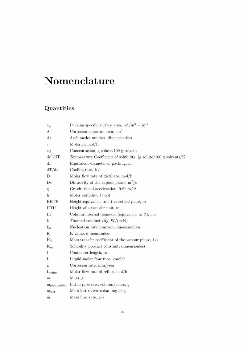
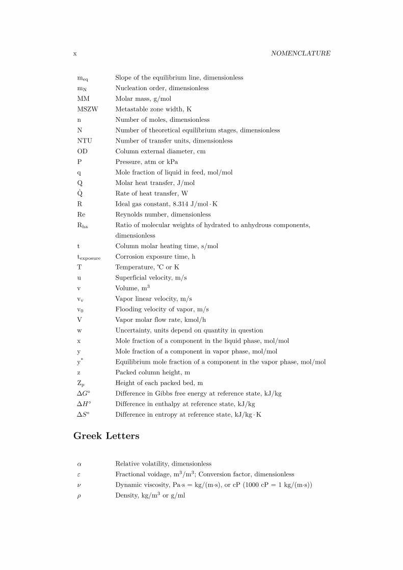
Nomenclature ixQuantities . . . . . . . . . . . . . . . . . . . . . . . . . . . . . . . . . . . . . . ixGreek Letters . . . . . . . . . . . . . . . . . . . . . . . . . . . . . . . . . . . . xSubscripts . . . . . . . . . . . . . . . . . . . . . . . . . . . . . . . . . . . . . . xiAcronyms . . . . . . . . . . . . . . . . . . . . . . . . . . . . . . . . . . . . . . xi
1 Introduction 1
2 Background 42.1 Boiling in the Subcooled Liquid Region . . . . . . . . . . . . . . . . . . 42.2 Vapor-Liquid Equilibrium (VLE) . . . . . . . . . . . . . . . . . . . . . . 52.3 Phase Diagrams . . . . . . . . . . . . . . . . . . . . . . . . . . . . . . . . 5
2.3.1 Tie-Lines . . . . . . . . . . . . . . . . . . . . . . . . . . . . . . . 62.4 Distillation . . . . . . . . . . . . . . . . . . . . . . . . . . . . . . . . . . 62.5 Azeotropes . . . . . . . . . . . . . . . . . . . . . . . . . . . . . . . . . . 8
3 Literature Review 93.1 Azeotropic Distillation . . . . . . . . . . . . . . . . . . . . . . . . . . . . 93.2 Extractive Distillation . . . . . . . . . . . . . . . . . . . . . . . . . . . . 103.3 Pressure-Swing Distillation . . . . . . . . . . . . . . . . . . . . . . . . . . 113.4 Batch Mode . . . . . . . . . . . . . . . . . . . . . . . . . . . . . . . . . . 133.5 Heat-Integrated Distillation Columns . . . . . . . . . . . . . . . . . . . . 13
3.5.1 Heat-Integrated PSD . . . . . . . . . . . . . . . . . . . . . . . . . 14
ii

CONTENTS iii
3.6 Reflux Ratio . . . . . . . . . . . . . . . . . . . . . . . . . . . . . . . . . 153.7 HETP Correlations . . . . . . . . . . . . . . . . . . . . . . . . . . . . . . 153.8 Outcome of the Literature Review . . . . . . . . . . . . . . . . . . . . . 15
4 The Effect of Metastability on Crystallization 174.1 Crystallization Results and Discussion . . . . . . . . . . . . . . . . . . . 184.2 Metastability . . . . . . . . . . . . . . . . . . . . . . . . . . . . . . . . . 18
4.2.1 Metastability Experimental Method . . . . . . . . . . . . . . . . 204.2.2 Formulation of Metastability & Equilibrium . . . . . . . . . . . . 204.2.3 Metastability Results and Discussion . . . . . . . . . . . . . . . . . 214.2.4 Metastability Conclusions . . . . . . . . . . . . . . . . . . . . . . 25
5 Distillation Simulation 265.1 Thermodynamic Models . . . . . . . . . . . . . . . . . . . . . . . . . . . 265.2 Simulation Setup . . . . . . . . . . . . . . . . . . . . . . . . . . . . . . . . 275.3 Simulation Results . . . . . . . . . . . . . . . . . . . . . . . . . . . . . . 28
5.3.1 Pressure-Swing Distillation . . . . . . . . . . . . . . . . . . . . . 285.3.2 Single-Column Distillation . . . . . . . . . . . . . . . . . . . . . . 34
5.4 Simulation Conclusion . . . . . . . . . . . . . . . . . . . . . . . . . . . . 34
6 Apparatus Design 366.1 Column Pressure . . . . . . . . . . . . . . . . . . . . . . . . . . . . . . . . 376.2 Experimental Setup Components . . . . . . . . . . . . . . . . . . . . . . . 37
6.2.1 Estimation of Mass Loss due to Corrosion . . . . . . . . . . . . . 386.3 Output Analysis . . . . . . . . . . . . . . . . . . . . . . . . . . . . . . . 39
6.3.1 Non-Applicability of Raoult’s Law . . . . . . . . . . . . . . . . . 406.3.2 Determining xHCl . . . . . . . . . . . . . . . . . . . . . . . . . . . 40
7 Column Geometry 427.1 Number of Stages . . . . . . . . . . . . . . . . . . . . . . . . . . . . . . . 427.2 Column Height . . . . . . . . . . . . . . . . . . . . . . . . . . . . . . . . 43
7.2.1 Method of Transfer Units . . . . . . . . . . . . . . . . . . . . . . 437.2.2 Empirical Correlations . . . . . . . . . . . . . . . . . . . . . . . . 45
7.3 Column Diameter . . . . . . . . . . . . . . . . . . . . . . . . . . . . . . . 487.4 Location of Feed Stage . . . . . . . . . . . . . . . . . . . . . . . . . . . . 48
8 Measurement and Control 508.1 Temperature Measurement . . . . . . . . . . . . . . . . . . . . . . . . . 508.2 Column Heating . . . . . . . . . . . . . . . . . . . . . . . . . . . . . . . . 518.3 Control System . . . . . . . . . . . . . . . . . . . . . . . . . . . . . . . . . 51
8.3.1 Schmitt Trigger . . . . . . . . . . . . . . . . . . . . . . . . . . . . . 518.3.2 PID Control . . . . . . . . . . . . . . . . . . . . . . . . . . . . . 52

iv CONTENTS
8.3.3 Electrical Design . . . . . . . . . . . . . . . . . . . . . . . . . . . 56
9 Apparatus Operation 589.1 Experimental Procedure . . . . . . . . . . . . . . . . . . . . . . . . . . . 58
10 Distillation Experimental Results and Discussion 6010.1 Analysis of the Column Outputs . . . . . . . . . . . . . . . . . . . . . . 60
10.1.1 Comparison of Experimental Results and Simulation Results . . 6210.2 Weaknesses & Limitations in the Results . . . . . . . . . . . . . . . . . . 62
10.2.1 Corrosion Product . . . . . . . . . . . . . . . . . . . . . . . . . . 6210.2.2 Vapour Pressure of the Vapour Phase . . . . . . . . . . . . . . . 62
10.3 Uncertainty Analysis . . . . . . . . . . . . . . . . . . . . . . . . . . . . . 6410.3.1 Systematic Error . . . . . . . . . . . . . . . . . . . . . . . . . . . 6410.3.2 Random Error . . . . . . . . . . . . . . . . . . . . . . . . . . . . 6410.3.3 Method of Kline & McClintock . . . . . . . . . . . . . . . . . . . 65
10.4 Distillation Conclusions and Recommendations . . . . . . . . . . . . . . 66
11 Conclusions and Recommendations 68
References 70
Appendix A Scripts 76A.1 McCabe-Thiele Method . . . . . . . . . . . . . . . . . . . . . . . . . . . 76A.2 Method of Kline & McClintock . . . . . . . . . . . . . . . . . . . . . . . 80
Appendix B Crystallization Results 86

Abstract
An atmospheric-pressure distillation system is designed and constructed to partiallyseparate hydrochloric acid and water. The system concentrates HCl(aq) between theelectrolyzer and hydrolysis steps of the Copper-Chlorine (Cu-Cl) cycle. Thus, the systempartially recycles HCl(aq), thereby decreasing the total operating cost of the cycle. Theseparation is only partial, as the mixture is unable to cross the azeotrope with onlya single pressure. The distillation system consists primarily of one packed distillationcolumn, which employs heating tapes and thermocouples to achieve a desired axialtemperature profile. The column can be operated in batch or continuous mode.
After performing physical distillation experiments, it is found that feeds less thanazeotropic concentration are separated into H2O(l) and highly-concentrated HCl(aq) (albeitat less than azeotropic concentration). Feeds greater than azeotropic concentration arenot investigated as they are extremely corrosive (rich in HCl) and would likely destroythe apparatus. Corrosion product is prevalent in the bottoms product; it is a source oferror that is partially mitigated by filtration.
No correlation is found between feed concentration and output concentration. That is,the distillate is H2O(l) and the bottoms is HCl(aq) near azeotropic concentration; as longas the feed concentration is any value less than azeotropic. In other words, the degree ofseparation is found to be independent of the feed concentration, for feed concentrationsless than azeotropic. The bottoms concentration varies from experiment to experiment,but does so randomly, likely the result of corrosion impurities affecting the calculation ofits concentration.
A simulation of pressure-swing distillation (PSD) is also performed to help determinethe feasibility of HCl-H2O separation and the degree of separation. Furthermore, aninvestigation into metastability and its effect on the crystallization of CuCl2 from HCl(aq)
solutions is presented in Chapter 4.
v

Acknowledgments
Dr. K. Pope, Dr. M. A. Rosen and Dr. O. A. Jianu are very gratefully acknowledged fortheir advice and guidance throughout this project. The financial assistance of the NaturalSciences and Engineering Research Council of Canada (NSERC), Ontario Research Fund(ORF) and Canadian Nuclear Laboratories (CNL) is gratefully acknowledged.
vi

List of Figures
1.1 Schematic of the Cu-Cl cycle [2] . . . . . . . . . . . . . . . . . . . . . . 2
2.1 Example Phase Diagram . . . . . . . . . . . . . . . . . . . . . . . . . . . 62.2 Distillation Example . . . . . . . . . . . . . . . . . . . . . . . . . . . . . . 7
3.1 Azeotropic Distillation Example [7] . . . . . . . . . . . . . . . . . . . . . 10
4.1 Hysteresis Loop of Metastability . . . . . . . . . . . . . . . . . . . . . . 194.2 Experimental Data on MSZW of CuCl2 in H2O . . . . . . . . . . . . . . 224.3 Effect of Cooling Rate on MSZW for CuCl2 in H2O . . . . . . . . . . . 234.4 Solubility of CuCl2 Dissolving in HCl Solutions of Different Molarities . 24
5.1 COCO (UNIQUAC) Phase Diagram at 1 bar . . . . . . . . . . . . . . . . 275.2 Chemcad Phase Diagram . . . . . . . . . . . . . . . . . . . . . . . . . . 305.3 Chemcad Process Flow Diagram . . . . . . . . . . . . . . . . . . . . . . 305.4 Simulation Results: Tray Compositions . . . . . . . . . . . . . . . . . . 335.5 Chemcad process flow diagram of single column distillation. . . . . . . . 34
6.1 Output Chamber Detail . . . . . . . . . . . . . . . . . . . . . . . . . . . 386.2 Bottoms including corrosion product . . . . . . . . . . . . . . . . . . . . . 41
7.1 McCabe-Thiele Method . . . . . . . . . . . . . . . . . . . . . . . . . . . 437.2 Equilibrium Concentrations . . . . . . . . . . . . . . . . . . . . . . . . . 447.3 Plot of 1/(y∗
i − yi) vs. y . . . . . . . . . . . . . . . . . . . . . . . . . . . 44
8.1 Thermocouple locations and temperature zones . . . . . . . . . . . . . . 508.2 Control diagram for n temperature zones . . . . . . . . . . . . . . . . . 538.3 Schmitt trigger flowchart . . . . . . . . . . . . . . . . . . . . . . . . . . 538.4 PID control flowchart . . . . . . . . . . . . . . . . . . . . . . . . . . . . 548.5 Electrical control schematic . . . . . . . . . . . . . . . . . . . . . . . . . . 57
vii

List of Tables
4.1 Nucleation Order and Nucleation Rate Constants for Several HCl Concen-trations . . . . . . . . . . . . . . . . . . . . . . . . . . . . . . . . . . . . 22
4.2 Nucleation Order and Rate for CuCl2 in H2O-HCl . . . . . . . . . . . . 23
5.1 Simulation Results: Stream Compositions . . . . . . . . . . . . . . . . . 285.2 Simulation Results: LPC Distillation Profile . . . . . . . . . . . . . . . . 295.3 Simulation Results: HPC Distillation Profile . . . . . . . . . . . . . . . . . 315.4 Simulation Results: LPC Tray Composition Data . . . . . . . . . . . . . . 315.5 Simulation Results: HPC Tray Composition Data . . . . . . . . . . . . . 325.6 Single-Column Simulation Results . . . . . . . . . . . . . . . . . . . . . 34
6.1 Corrosion Resistance, Data from [41] . . . . . . . . . . . . . . . . . . . . 386.2 Parameters for Calculating mlost . . . . . . . . . . . . . . . . . . . . . . 39
7.1 Parameters for Calculating HTU . . . . . . . . . . . . . . . . . . . . . . 467.2 Parameters used in Equation 7.9 to Calculate DV . . . . . . . . . . . . . 467.3 Values used to Calculate Empirical Correlations for HETP . . . . . . . . . 477.4 Results of Empirical Correlations for HETP . . . . . . . . . . . . . . . . . 477.5 Parameters for Calculating Column Diameter . . . . . . . . . . . . . . . 49
8.1 Parameters for Calculating Column Heat Input . . . . . . . . . . . . . . 52
10.1 Measured Densities and Calculated Concentrations . . . . . . . . . . . . . 6110.2 Comparison of Experimental Results and Simulation Results . . . . . . 6310.3 Instrument Uncertainties . . . . . . . . . . . . . . . . . . . . . . . . . . . 6410.4 Uncertainties, following the approach of Kline & McClintock . . . . . . 66
B.1 Crystallization Results . . . . . . . . . . . . . . . . . . . . . . . . . . . . 86
viii
Nomenclature
Quantities
ap Packing specific surface area, m2/m3 = m-1
A Corrosion exposure area, cm2
Ar Archimedes number, dimensionlessc Molarity, mol/LcN Concentration, g solute/100 g solventdc*/dT Temperature Coefficient of solubility, (g solute/100 g solvent)/Kde Equivalent diameter of packing, mdT/dt Cooling rate, K/sD Molar flow rate of distillate, mol/hDV Diffusivity of the vapour phase, m2/sg Gravitational acceleration, 9.81 m/s2
h Molar enthalpy, J/molHETP Height equivalent to a theoretical plate, mHTU Height of a transfer unit, mID Column internal diameter (equivalent to Φ), cmk Thermal conductivity, W/(m·K)kN Nucleation rate constant, dimensionlessK K-value, dimensionlessKV Mass transfer coefficient of the vapour phase, 1/sKsp Solubility product constant, dimensionlessl Condenser length, mL Liquid molar flow rate, kmol/hL Corrosion rate, mm/yearLreflux Molar flow rate of reflux, mol/hm Mass, gmpipe, initial Initial pipe (i.e., column) mass, gmlost Mass lost to corrosion, mg or gm Mass flow rate, g/s
ix
x NOMENCLATURE
meq Slope of the equilibrium line, dimensionlessmN Nucleation order, dimensionlessMM Molar mass, g/molMSZW Metastable zone width, Kn Number of moles, dimensionlessN Number of theoretical equilibrium stages, dimensionlessNTU Number of transfer units, dimensionlessOD Column external diameter, cmP Pressure, atm or kPaq Mole fraction of liquid in feed, mol/molQ Molar heat transfer, J/molQ Rate of heat transfer, WR Ideal gas constant, 8.314 J/mol ·KRe Reynolds number, dimensionlessRha Ratio of molecular weights of hydrated to anhydrous components,
dimensionlesst Column molar heating time, s/moltexposure Corrosion exposure time, hT Temperature, or Ku Superficial velocity, m/sv Volume, m3
vv Vapor linear velocity, m/sv0 Flooding velocity of vapor, m/sV Vapor molar flow rate, kmol/hw Uncertainty, units depend on quantity in questionx Mole fraction of a component in the liquid phase, mol/moly Mole fraction of a component in vapor phase, mol/moly* Equilibrium mole fraction of a component in the vapor phase, mol/molz Packed column height, mZp Height of each packed bed, m∆G° Difference in Gibbs free energy at reference state, kJ/kg∆H° Difference in enthalpy at reference state, kJ/kg∆S° Difference in entropy at reference state, kJ/kg ·K
Greek Letters
α Relative volatility, dimensionlessε Fractional voidage, m3/m3; Conversion factor, dimensionlessν Dynamic viscosity, Pa·s = kg/(m·s), or cP (1000 cP = 1 kg/(m·s))ρ Density, kg/m3 or g/ml

xi
ρmetal Column metal density, g/cm3
σ Molecular diameter, Å; Collision diameter, ÅσL Surface tension, mN/m or N/mΦ Column internal diameter (equivalent to ID), mω Interfacial surface area per unit volume of column, m2/m3
Ω Molecular property, dimensionless, ≈1
Subscripts
aq Aqueous stateb Bottomsd Distillatef Feedg Gas phaseG Gas statei Component i, (chemical species i)l Liquid phaseL Liquid statev Vapor phaseV Vapor state
Acronyms
ED Extractive distillationEES Engineering Equation Solver (software)HCl Hydrogen ChlorideHPC High-pressure columnLPC Low-pressure columnPPAQ Partial-Pressure of Aqueous Solutions (Thermodynamic model)PSD Pressure-swing distillationSRK Soave-Redlich-Kwong (Thermodynamic model)TAC Total annual costVLE Vapor-liquid equilibrium

Chapter 1
Introduction
Alternative energy (e.g., solar, wind, hydrogen, geothermal) is of vital importance becausethe world’s supply of fossil fuels is limited and the production/consumption of fossil fuelsproduces pollution. Hydrogen (H2) is a promising alternative to fossil fuels because itdoes not produce CO2 or other pollutants (e.g., CO, NOx, SOx), when used as an energysource. Since H2 does not occur naturally, it must be produced by techniques suchas steam-methane reforming. However, steam-methane reforming is disadvantageousbecause it requires natural gas, which is a fossil fuel, and because CO is produced as abyproduct [1].
The Copper-Chlorine (Cu-Cl) cycle is a novel 4-step thermochemical cycle to generatehydrogen, presented in Equations 1.1 to 1.4 [2] and Figure 1.1.
1 (Electrochemical) : 2CuCl(aq) + 2HCl(aq) → 2CuCl2(aq) + H2(g) 25− 90(1.1)
2 (Drying) : 2CuCl2(aq) → 2CuCl2(s) 60− 200(1.2)
3 (Hydrolysis) : 2CuCl2(s) + H2O(g) ↔ Cu2OCl2(s) + 2HCl(g) 350− 450(1.3)
4 (Thermolysis) : Cu2OCl2(s) → 2CuCl(l) + 1/2 O2(g) 520 (1.4)
The HCl(aq) concentration step (which occurs between the hydrolysis step (step 3)and electrochemical step (step 1)) is not explicitly listed in [2], however, it may beexpressed as:
HCl(aq)Concentration : 2HCl(aq) → 2HCl(g) + H2O(g) 110 (1.5)
HCl is in the aqueous state (negating the vapour pressure due to volatility) inEquation 1.1 because the reaction temperature is less than the boiling point of HCl(aq).HCl is in the gaseous state in Equation 1.3 because the reaction temperature is greaterthan the boiling point of HCl(aq).
1

2 CHAPTER 1. INTRODUCTION
In Equation 1.5, the separation of HCl and H2O is assumed to be complete. Since allHCl is separated from H2O, and the temperature is ~110, both HCl and H2O would bein the gaseous state (since 110 is greater than the boiling points of both pure HCl andpure H2O (at 1 atm pressure)). Therefore, the subscript g is written for both productsin Equation 1.5 to indicate gaseous state.
However, if the HCl-H2O separation described in Equation 1.5 is only partial, thenthe products would be: HCl(aq), HCl(g), and H2O(g).
The Cu-Cl cycle is advantageous over other hydrogen production cycles because ofits lower temperature requirements. Waste heat (an industrial byproduct) can be usedto drive the reactions of the Cu-Cl cycle. Distillation is relevant to the Cu-Cl cycle as itincreases the concentration of the HCl(g) produced in step 3, recycles it, and makes itsuitable for use as a reactant in step 1.
Distillation can be used to concentrate hydrochloric acid HCl(aq) between the hydrol-ysis and electrolyzer steps of the Cu-Cl cycle as shown in Figure 1.1. HCl concentration(via distillation using waste heat) occurs at the location of the condenser/evaporator onFigure 1.1, HCl(g)/steam → HCl(aq).
Figure 1.1: Schematic of the Cu-Cl cycle [2].
The problem addressed in this thesis, is recycling HCl within the Cu-Cl cycle, byseparating HCl from water. Recycling HCl is needed to maintain the Cu-Cl cycle’sefficiency. Therefore, an economical method of concentrating HCl(aq) is needed.
The objective of this thesis to demonstrate that the concentration of HCl(aq) can beincreased (and thus a partial separation can be performed) using a single distillationcolumn, provided that the feed concentration is less than azeotropic (0.11 mole fractionHCl).

3
The scope of this thesis comprises: a review of existing literature, simulation ofdistillation, design calculations, component and material selection, programming, columnassembly, column operation, output analysis (e.g., determining the concentration ofHCl(aq) in the output products) and the providing of recommendations. Work per-formed in this thesis for HCl-water separation includes: simulation, calculations, design,programming, construction, column operation and output analysis.
Optimization (e.g., increasing energy efficiency of the distillation column) falls outsidethe scope of this thesis, since the focus of this thesis is feasibility.
Other researchers, such as Fayazuddin [3], have used software to simulate a pressure-swing distillation system. However, to the author’s knowledge, no documented attempthas been made to physically construct an HCl-water distillation system. Aghahosseini [4]concluded that pressure-swing distillation is not economical without heat-integration. Liet al. [5] performed an Aspen simulation for heat-integrated pressure-swing distillation(PSD) on an ethylenediamine/water system and found that the heat-integration decreasesenergy consumption by 19.79% and decreases total annual cost by 15.30%. The work ofthese and other researchers is detailed in Chapter 3.
The feasibility of separating HCl from water with reasonable purity (i.e., the feasibilityof the separation from a chemical standpoint and from a construction standpoint) isdetermined using simulation software (Chapter 5) and design calculations (Chapter 6).Design calculations are made using analytical and empirical methods. One distillationcolumn, operating at atmospheric pressure is built. A single-pressure column is adequatefor the purpose of this thesis, because it produces pure HCl (but not pure water), providedthe feed concentration of HCl is greater than the azeotropic concentration. The outputof the column is analyzed using the techniques described in Section 6.3.
This thesis describes the the theoretical and experimental work performed for concen-trating HCl(aq). The theoretical work includes a review of existing literature, a simulationof the system, and the calculation of column parameters (e.g., length, diameter, heatduty). Crystallization increases the energy efficiency of the Cu-Cl cycle because, incontrast to spray drying, it does not require a pump to force the mixture through anozzle. Distillation reduces the operating cost of the Cu-Cl cycle by recycling HCl(aq).
Results are not consolidated, but rather presented in their corresponding section.This is done so that results may be presented alongside their context. Crystallizationand metastability results are presented in Section 4.1, simulation results are presented inSection 5.3, and distillation experimental results are presented in Chapter 10.

Chapter 2
Background
2.1 Boiling in the Subcooled Liquid Region
Most liquids are partially vapourized when the temperature and pressure are in thesubcooled liquid region (i.e., when the temperature is below the boiling temperature andthe pressure is above the boiling pressure). This partial vapourization is caused by anunequal distribution of molecular kinetic energies in a specimen of uniform temperature.Temperature is the average kinetic energy of molecules; the standard deviation ofmolecular kinetic energies can be quite large. Some molecules have sufficient kineticenergy to overcome the intermolecular bonds (intermolecular forces) that hold them inthe liquid state, and consequently enter the gaseous (vapour) state. Hence, the liquidhas a vapour (of the same chemical formula) above it even though the temperature andpressure are in the subcooled liquid region. The vapour phase above the liquid phaseexerts a pressure, known as vapour pressure.
It is due to the unequal distribution of molecular kinetic energies in a specimen ofuniform temperature (resulting in some molecules having sufficient kinetic energy toovercome the intermolecular forces which hold them in the liquid state and enter thevapour state), that water at room temperature gradually evaporates.
The notion of a subcooled liquid region (i.e., only liquid and no vapour if thetemperature is below the boiling temperature and the pressure is above the boilingpressure) belongs to an idealized thermodynamic model which assumes that each andevery molecule in a specimen of uniform temperature has identical kinetic energy. Thisthermodynamic model is useful in many contexts, but it cannot be used to describedistillation.
4

2.2. VAPOR-LIQUID EQUILIBRIUM (VLE) 5
2.2 Vapor-Liquid Equilibrium (VLE)
Different chemical species have different standard deviations of molecular kinetic energyfor the same temperature. Those which have a larger fraction of molecular kineticenergies in the gaseous state (i.e., above a certain threshold), at a given temperature,exert a higher vapour pressure.
The greater the vapour pressure exerted by a given chemical species at a giventemperature, the greater the volaltility. Liquid chemical species which exert a vapourpressure (most of them) are said to be volatile. The K-value for component i, Ki, isthe ratio of the mole fraction in the vapour phase (yi) to the mole fraction in the liquidphase (xi).
Ki = yixi
(2.1)
If the temperature and chemical composition are held constant, then the rates ofvapourization and condensation are equal and the substance is said to be in vapour-liquidequilibrium (VLE), which is a type of dynamic equilibrium.
For a mixture of n components (i.e., chemical species), the total vapour pressure(above the mixture) is the sum of the vapour pressures of each component, as stated byDalton’s Law of Partial Pressures (Equation 2.2):
Ptotal =n∑i=1
Pi = P1 + P2 + ...+ Pn (2.2)
2.3 Phase Diagrams
Concentration is conventionally expressed as the mole fraction of the more volatilecomponent, as shown by Equation 2.3 (either as number between 0 and 1, or as apercentage).
Mole Fraction = Moles of the more volalitle component in a certain phase
Total moles in that same phase(2.3)
A phase diagram (Figure 2.1) shows the dew point temperature (when the vapourbegins to condense (upper curve)) and bubble point temperature (when the liquid beginsto boil (lower curve)) for binary mixture, as a function of concentration. In the regionbetween the curves, vapour and liquid exist simultaneously in VLE.

6 CHAPTER 2. BACKGROUND
Figure 2.1: Phase diagram for a fictitious binary mixture of A and B, where B is themore volatile component.
2.3.1 Tie-Lines
For a given temperature, the concentration (of the more volatile component) in thevapour and liquid phases can be found via the tie-line method. The method consistsof drawing a horizontal line at the desired temperature, then reading the horizontalcoordinate (i.e., concentration) of the point where it intersects the bubble point curve(liquid concentration) and the dew point curve (vapour concentration).
Figure 2.1 shows the tie-line (horizontal line at Tx), vapour concentration cV, andliquid concentration cL, for a temperature Tx.
2.4 Distillation
Distillation is the separation of two or more chemical species based on vapour pressure,boiling points and relative volatility.
In order for distillation to be feasible, the vapour pressure (and consequently y) ofeach component must be different, in a mixture of uniform temperature. For example, fora mixture of HCl and H2O at room temperature, HCl exerts a larger vapour pressure andconsequently has a larger y. Symbolically, this is: @ Troom : yHCl > yH2O, PHCl > PH2O.
The greater the difference in y for two components, the greater the relative volatility,α. A greater α means that fewer equilibrium stages are required to achieve a given

2.4. DISTILLATION 7
separation (a given purity). The relative volatility for two components, i and j, can alsobe expressed as the ratio of their K-values. Usually, the larger K-value is written in thenumerator, such that α ≥ 1.
αij = Ki
Kj= yi/xiyj/xj
(2.4)
For a component i, in a mixture, yi increases with temperature. yi and Ki increasewith temperature, whereas xi decreases with temperature. A different vapour-liquidequilibrium exists at a different temperature. For this reason, temperature varies fromstage to stage along the length of a distillation column. Typically, temperature is highestat the bottom of the column and decreases with height.
In distillation, the vapour of a certain concentration (usually expressed as molefraction of the more volatile component) at given stage (or theoretical plate) rises dueto buoyancy and due to the slight pressure differential along the column height. Thebottom of the column is usually hottest so that it will be at the highest pressure. Thistemperature differential creates a corresponding pressure differential which helps thevapour phase rise to the next stage. When the vapour travels upward and reaches thenext stage, which is colder than the stage below it, the vapour partially condenses to aliquid of the same concentration. At this new temperature there is still vapour abovethe liquid (i.e., VLE is occuring). However, the vapour at the new stage is at a differentconcentration than the vapour at the previous stage. This vapour also rises to the nextstage and condenses. In this way, as shown in Figure 2.2, separation is achieved.
Figure 2.2: Distillation column with 7 stages for a fictitious binary mixture.

8 CHAPTER 2. BACKGROUND
In Figure 2.2, the concentrations of vapour (V) and liquid (L) are expressed inpercentages as mole fractions of the more volatile component. For example, at the feedstage (stage 5): Vmore volatile = 30%∴ Vless volatile = 100% - 30% = 70%, andLmore volatile = 10% ∴ Lless volatile = 100% - 10% = 90%.
2.5 Azeotropes
An azeotrope occurs when the concentration of the vapour and liquid phase are equal,thus making further separation by typical distillation techniques impossible. Therefore,an azeotrope only occurs at a certain concentration (i.e., the azeotropic concentration).At other concentrations, no azeotrope is present. The azeotropic concentration may varywith pressure. On a phase diagram, an azeotrope is indicated by the dew point andbubble point curves touching.
Not all mixtures have azeotropes, however HCl-H2O has an azeotrope at about 11.1%mole fraction HCl at a pressure of 1 atm [6].

Chapter 3
Literature Review
The purpose of the literature review is to obtain a thorough understanding of whathas already been accomplished in field of pressure-swing distillation (especially how itpertains the Cu-Cl cycle). Topics examined include: azeotropic distillation, extractivedistillation, pressure-swing distillation, batch mode, heat-integration distillation columns,reflux ratio and HETP (height equivalent to a theoretical plate) correlations.
A significant portion of the research cited in the literature review does not directlypertain to HCl-water separation, however, it is still relevant, as the principles (pressure-swing distillation, heat) and outcomes (lower TAC (total annual cost), energy savings,higher purities, etc.) detailed therein are applicable to azeotropic HCl-water systems.
Although the Cu-Cl Cycle requires the separation of a binary mixture (namely HCl-water), the sources in this review are useful as they provide insight into heat integrationwhich results in considerable energy savings.
3.1 Azeotropic Distillation
Azeotropic distillation of chemical species A and B requires an entrainer, E, which formsanother azeotrope with either A or B. In the first column, E is mixed with A + B. PureA is separated from the resulting azeotropic mixture B + E. Pure A exits via the bottomand B + E exits via the top and flows into a decanter. In the decanter, two insolubleliquid layers occur; one rich in B, the other rich in E. The layer rich in E returns to thefirst column, and the layer rich in B travels to the second column where some pure B isseparated from the azeotropic mixture B + E. Pure B exits via the bottom and B + Eexits via the top and returns to the decanter [7].
An example of azeotropic distillation to separate water and acetic acid with ester asthe entrainer is given in Figure 3.1 [7].
9

10 CHAPTER 3. LITERATURE REVIEW
Figure 3.1: Azeotropic Distillation Example [7]
In azeotropic distillation, it is imperative that a suitable entrainer is selected. Asuitable entrainer is one that allows the formation of the insoluble liquid layers, sinceinsolubility is necessary for successful separation. That is, one of the chemical species tobe separated must be insoluble in the entrainer.
Knapp and Doherty [8] discuss conventional pressure-swing distillation (PSD) forpressure-sensitive (where the azeotropic concentration changes with pressure) binaryazeotropes, such as HCl-water, which resembles that encountered in the Cu-Cl cycle.PSD for ternary mixtures as well as a new PSD process for pressure-insensitive azeotropeswhich requires an entrainer to create a pressure-sensitive azeotrope, are discussed. Chienet al. [9] investigated azeotropic distillation of an isopropyl alcohol (IPA)-water systemwith use of cyclohexane (CyH) as an entrainer. A 2-column and 3-column method arecompared. It is concluded that the 2-column method is less costly.
3.2 Extractive Distillation
Extractive distillation, which separates a close-boiling binary mixture of A & B, requiresa solvent with a boiling point substantially higher than those of both A and B. A andB must both be soluble in the solvent. The solvent breaks the azeotrope because itchanges the relative volatility of A to B [10]. In the first column, A is separated fromthe solution of B and the solvent. The solution of B and the solvent is then pumpedto the second column, in which B is separated from the solvent. Finally, the recoveredsolvent is returned to the first column. The solvent used in extractive distillation mustbe completely removed in each column so that purity is not affected.
Although similar to azeotropic distillation, extractive distillation is simpler in most

3.3. PRESSURE-SWING DISTILLATION 11
cases. This is because extractive distillation breaks the azeotrope (whereas azeotropicdistillation does not), and extractive requires less apparatus (e.g., azeotropic distillationrequires a decanter whereas extractive distillation does not).
Numerous researchers [11–14] have found PSD to have a lower cost than extractivedistillation. This is probably because extractive distillation requires the use and extractionof a solvent, which adds more components, steps and apparatus to the separation system.However, other researchers [15,16] have found extractive distillation to have the lowercost. Since the researchers cited used different chemicals (that variable is uncontrolled),it is also evident that the chemicals to be separated play a major role in the cost.
Luyben [15] investigated PSD and extractive distillation for a maximum-boilingazeotrope of acetone and choloroform. It is concluded that PSD has a TAC of $4,327,000,whereas extractive distillation has a substantially lower TAC of $952,700. Luyben [16]compared extractive distillation and PSD for an acetone-methanol system. The extractivesystem was found to have 15% lower TAC. Wang et al. [11] compared extractive distillationand PSD for a tetrahydrofuran (THF)-ethanol system. They found that PSD is moreeconomical (contrary to [16], although different chemicals are used) and also giveshigher purities of the outputs. The capital costs of PSD and extractive distillation, are$0.9310× 10⁶ and $0.9450× 10⁶, respectively. Muñoz et al. [12] performed a simulationwith Aspen HYSYS to compare the separation of a system 12,000 Tm/year of 52 mole%isobutyl alcohol and 48 mole% isobutyl acetate, via extractive distillation (with n-butylpropionate as an entrainer), and via PSD. They concluded PSD has a lower TAC thanextractive distillation (1.123×10⁶ USD/year and 1.508×10⁶ USD/year, respectively). Itis also concluded that PSD has lower fixed capital investment than extractive distillation(2.492×10⁶ USD and 3.924×10⁶ USD, respectively). Lladosa et al. [13] compared PSDand extractive distillation (ED) for a mixture of 50 mol% di-n-propyl ether and 50 mol%n-propyl alcohol, using Aspen HYSYS. It is found that PSD has a substantially lowerfixed capital investment (1.205×10⁶ USD and 1.925×10⁶ USD, for PSD & ED (extractivedistillation), respectively), as well as lower TAC (514.99×10³USD/year and 730.13×10³
USD/year, for PSD & ED, respectively), compared to extractive distillation. Hosgoret al. [14] performed a comparison between extractive distillation and PSD (with andwithout heat integration) on a simulated system of methanol-chloroform in Aspen Plusand Aspen Dynamics. They found PSD (TAC = 0.7269 × 10⁶$/yr) to be less costlythan extractive distillation (TAC = 2.2174 × 10⁶$/yr).
3.3 Pressure-Swing Distillation
QVF Corporation [17] investigated Dual-Pressure Distillation (i.e., pressure-swing dis-tillation (PSD)) for HCl-water systems. A plot of azeotropic HCl concentration as a

12 CHAPTER 3. LITERATURE REVIEW
function of pressure shows that azeotropic concentration decreases with pressure. Suchdata is vital for selecting the PSD pressures. A process flow diagram of a proposed PSDsystem is also provided. Fayazuddin [3] investigated PSD of HCl-water systems for theCu-Cl cycle for hydrogen production using simulations in CHEMCAD software. PSDis found to be less costly than azeotropic distillation since no entrainer is required. Atpressures of 1 atm and 20 atm, an HCl purity of 80.4% is obtained. At pressures of0.1 atm and 10 atm, an HCl purity of 76.6% is obtained. Aghahosseini [4] investigatedazeotropic mixture separation for HCl-water systems, including PSD. It was concludedthat PSD is not economically viable without heat exchange between the high-pressure(hotter) column and low-pressure (colder) column. Aghahosseini [4] also investigatedother methods for azeotropic separation such as extractive distillation and concludedthat for extractive distillation, the reflux flow rate should be minimized as excessivereflux dilutes the entrainer, thereby decreasing its effectiveness. Palomino et al. [18]investigated PSD for an ethanol-water system. First, the concentration of ethanol wasincreased from 80% v/v to 95% v/v, using simple distillation. Then the concentration ofethanol was increased from 95% v/v to 97% v/v via PSD. Wang et al. [19] examined asystem of n-heptane and isobutanol which forms both minimum- and maximum-boilingazeotropes, depending on pressure. The LPC is set at atmospheric pressure, whichresults in two different PSD processes: conventional PSD (CPSD) and unusual PSD(UPSD). CPSD forms minimum-boiling azeotropes under both low and high pressures.UPSD forms minimum-boiling azeotropes under low pressure and maximum-boilingazeotropes under high pressure. It is concluded that CPSD has a lower TAC than UPSD,whereas UPSD has better dynamic control than CPSD. Fulgueras et al. [20] performed asimulation to separate ethylenediamine (EDA) from aqueous solution using PSD withheat integration for low-high (LP+HP) and high-low (HP+LP) configurations. Theminimum number of column stages is achieved when the low and high pressures are 100mmHg and 4909.6 mmHg, respectively.
Phimister and Seider [21] discuss PSD using only one column, which is alternatedbetween the low and high pressures (known as semi-continuous PSD). According to [21],cost savings can be achieved by using one column with alternating pressures. A simulationis performed for a tetrahydrofuran-water system. It is concluded that the cost decreasesby 22.5% - 32.5% when semi-continuous PSD (single-column) is used. However, withsemi-continuous PSD one must use larger feed tanks, perhaps a more complex controlsystem and also heat cannot be transferred between columns. These constraints diminishthe cost savings.

3.4. BATCH MODE 13
3.4 Batch Mode
A unit operation (such as distillation) may be operated in batch mode (discrete) orcontinuous mode. In batch mode, an amount feed is input to the column, and no morefeed is added until the initial amount is processed. In continuous mode, at steady-state,the sum of the mass flow rates into and out of the unit are constant. An advantage ofbatch mode is usually lower capital cost, because a feed pump is not required as the feedcan be input manually at the beginning of each batch.
Modla and Lang [22] examined batch PSD methods such as: rectifier, stripper, andmiddle vessel column. Two new configurations are proposed: double column batchrectifier (DCBR) and double column batch stripper (DCBS). DCBR and DCBS arefound to be advantageous over the preexisting configurations, due to the presence ofonly one production step, no change in pressure, almost steady-state operation of bothcolumn section, and thermal integration of the columns. Repke et al. [23] investigatedbatch PSD for an acetonitrile-water system, using two modes of batch PSD; regularand inverted. The inverted batch mode is found to require less time per batch than theregular mode, for feeds with a small amount of light (low-density) component.
3.5 Heat-Integrated Distillation Columns
Heat-integration is employed in distillation systems (PSD and other types) to reduceenergy consumption and TAC. Generally, heat integration consists of a heat exchangerwhich transfers heat from an output of one column to an input of another column. Heatintegration increases the capital cost (because of the extra components, namely, the heatexchanger and accessories). However, the researchers [24–28] found that heat-integrationdecreases the TAC since less external heat is required.
Kiss and Olujic [24] investigated internally heat-integrated distillation columns(HIDiC), which can be used for simple distillation, as well as PSD. It is found thata HIDiC can realize a maximum of 70% energy savings over conventional distillationcolumns. Shahandeh et al. [25] performed a comparison between: HIDiC (Heat-IntegratedDistillation Column), VRC (Vapor Recompression Column) and CDiC (ConventionalDistillation Column). The comparison is performed on three mixtures: benzene-toluene,propane-propylene and methanol-water. The comparison is performed in terms of TAC(total annual cost). It is found that a CDiC is optimal for benzene-toluene, a VRC isoptimal for propane-propylene (44.1% decrease in TAC relative to CDiC), and a HIDiC isoptimal for methanol-water (3.4% decrease in TAC relative to CDiC, and 31.2% decreasein TAC relative to VRC). Ponce et al. [26] used Aspen Plus to compare the energyrequirements for a HIDiC ((heat-integrated distillation column) with and without heat
14 CHAPTER 3. LITERATURE REVIEW
panels) and a CDiC (Convential Distillation Column), for the separation of an ethanol-water mixture. Energy savings of approximately 77% in the boiler, are obtained, relativeto a CDiC when using a HIDiC with heat panels. Kiran and Jana [27] propose a PSDsystem which incorporates both HIDiC (heat-integrated distillation column) and VRC(vapour recompression column), to increase the energy efficiency of the system. The VRCensures that the temperature of the vapour in the HPC is at least 20 K hotter (minimumdifference in temperature) than the LPC. The combined HIDiC-VRC system has energysavings of approx. 29.5%, when simulated for a system of ethylacetate. Mulia-Soto etal. [28] simulated PSD with internal heat integration (IHIPSD) for separation of anethanol/water mixture. Using internally heat integrated PSD (IHIPSD), the total heatinput was reduced from 6.33 MW to 4.30 MW. The LPC is at 1 atm and the HPC is at10 atm.
3.5.1 Heat-Integrated PSD
Heat integration is especially benefical when combined with PSD, as it takes advantageof the temperature rise that occurs when the fluid is pressurized, by routing the resultingexcess heat (that would otherwise dissipate to the surroundings) from the HPC to LPC.Typically, heat integration consists of a heat exchanger which transfers heat from one ofthe HPC outputs to one of the LPC inputs. As the pressure of the HPC output dropsthrough the adiabatic heat exchanger, the fluid expands and cools, thus transferring heatto the LPC input and decreasing the reboiler duty of the LPC. Similar to Section 3.5, heatintegrated PSD is found to increase the capital cost (because of the extra components,namely, the heat exchanger and accessories), but is also found to decreases the TAC andenergy consumption since less external heat is required.
Abu-Eishah and Luyban [29] investigated energy consumption reduction of PSD fora tetrahydrofuran-water system. Heat integration and feed preheat were employed todecrease the energy consumption by approximately half. Cheng and Luyben [30] investi-gated heat integration for a ternary system of benzene-toluene-m-xylene and realizedenergy savings of 35%-45% depending on configuration. Li et al. [5] used Aspen Plusand Aspen Dynamics to simulate a partially heat-integrated pressure-swing distillationprocess for separating an ethylenediamine/water system. Partially heat-integrated PSDwas found to decrease energy consumption by 19.79% and decreases TAC by 15.30%.Kiran and Jana [31] discuss heat integration for PSD of bioethanol dehydration. Threemethods are compared: 1.) only heat integrated distillation column (HIDiC), 2.) idealhybrid HIDiC-VRC (Vapor Recompression Column, and 3.) conventional standalonePSD. The ideal hybrid HIDiC-VRC is found to be the optimal solution, with energysavings of 82.88% and TAC savings of 22.16%.

3.6. REFLUX RATIO 15
3.6 Reflux Ratio
Reflux ratio is the ratio of the amount product re-entering the column to the amount ofproduct leaving the top of the column as distillate. The use of reflux is not mandatory,however, a higher reflux ratio tends to result in a higher purity of the distillate as itpasses through the column several times before finally leaving.
Knapp [32] discusses reflux ratio, which is the ratio of the amount of reflux (condensedliquid from the vapour (“tops”)) that goes back down the column over the amount ofreflux which leaves the column as distillate. Higher reflux ratios typically yield higherpurity, but require more time to process a unit mass, since the net flow rate is lower (netflow = total - reflux). Maximum reflux is the reflux above which separation is impossible.Lee et al. [33] performed a simulation, using PRO/II with PROVISION release 8.3, ofPSD to separate a mixture of tetrahydrofuran (THF) and water. They found a refluxratio of 0.4 on both columns resulted in lowest reboiler duty, presumably saving energy.They achieved purities of 99.9 mole% for both THF and water. Although, one shouldremember that these purities are the result of simulations, real-world purities are likelylower.
3.7 HETP Correlations
The work of Wang et al. [34] includes an aggregation of empirical HETP correlationsfor packed columns from numerous researchers. These correlations give HETP interms of various parameters such as phase densities, phase velocities, phase dynamicviscosities and column diameter. The column height (z) is calculated in terms of HETPusing Equation 7.1. These correlations and the results generated by them are given inSection 7.2.2.
3.8 Outcome of the Literature Review
After performing the literature review, it is determined that although simulations exist [3],no pressure-swing distillation to separate HCl-water has been physically performed.Therefore, it is decided that the focus of this research is to separate HCl-water viadistillation. It is determined to avoid azeotropic distillation (using an entrainer and adecanter) and extractive distillation (using an additional solvent to break the azeotrope),as they require additional chemical species, additional separation step(s), and in thecase of azeotropic distillation; additional apparatus (namely the decanter), all of whichincreases cost and complexity.

16 CHAPTER 3. LITERATURE REVIEW
It is also determined to avoid the use of heat-integration because, although it resultsin energy savings and lower TAC in the long-term, it also increases the capital cost of thesystem (primarily due to the heat exchanger and associated piping). Since the systemdetailed in this thesis is of lab scale (and therefore is only used short-term, so decreasingcapital cost is the priority), it is not economically viable to employ heat-integration.

Chapter 4
The Effect of Metastability onCrystallization
Crystallization is necessary for the integration of the hydrolysis and electrolyzer unitsof the Cu-Cl cycle for hydrogen production. As shown by Figure 1.1, crystallization isemployed in the drying step of the Cu-Cl cycle to separate CuCl2 and water accordingto:
CuCl2(aq) → CuCl2(s) + H2O(l) (4.1)
CuCl2(s) travels to the hydrolysis reactor and H2O(l) travels to the electrolyzer, wherethey are inputs for their respective units. Crystallization is less energy intensive thanother methods to recover solids from solution, such as spray-drying, which requires apump to spray pressurized solution through a nozzle. Precipitation (of solids from liquidsolutions) relies on the fact that the solubility of a solute in a liquid solvent increaseswith temperature. Since crystallization is the only form of precipitation discussed in thischapter, the words crystallization and precipitation are used interchangeably.
In one set of experiments, performed at UOIT’s Clean Energy Research Laboratory,the solvent is heated to the high temperature, and the solute is added such that theconcentration at the high temperature is greater than the saturation concentration atthe low temperature. Upon cooling to the low temperature, the excess solute solidifies inthe form of crystals.
Another set of experiments, also performed at UOIT’s Clean Energy Research Labo-ratory, shows that the dissolution temperature (Td) and the crystallization temperature(Tmet) are not identical; the difference between them is the Metastable Zone Width(MSZW). This type of hysteresis is known as metastability. An understanding of metasta-bility, described in Section 4.2, is used to optimize and refine the crystallization process.
17

18 CHAPTER 4. THE EFFECT OF METASTABILITY ON CRYSTALLIZATION
4.1 Crystallization Results and Discussion
It is found that crystallization of CuCl2 does not occur at HCl concentrations > 9M.Chemicals are added in the following order: water, CuCl2, HCl(aq). Adding HCl(aq),despite there being negligible change in ambient temperature (e.g., negligible change intemperature due to enthalpy of mixing), causes crystallization to begin immediately. Thisis maybe due to CuCl2 reacting with HCl to form complexes [35]. Anhydrous copper (II)chloride is found to never crystallize from HCl(aq) solutions. There is also a relativelynarrow range of concentrations for which CuCl2 will crystallize; if the concentrationis below the range there will be no crystallization and the solution will remain liquid.Conversely, if the concentration exceeds the upper bound of the range, the solution willbe saturated, and there will be precipitate at all temperatures in the range. The resultsof the crystallization experiments are summarized in Table B.1. The volume of thesolvent (HCl(aq)) is 100 mL.
There is a narrow range of concentrations that will demonstrate crystallization. Ifthe initial concentration exceeds the upper bound of this range, the solution will besaturated and precipitation will occur instantly. Conversely, if the initial concentrationsfalls below the lower bound of this range, the solution will remain liquid upon cooling. Itis found that anhydrous copper (II) chloride does not crystallize, crystallization doesnot occur at concentrations > 9M, and HCl can cause near-instantaneous crystallizationwhen it is added to aqueous CuCl2 solution.
Crystallization is achieved frequently and consistently when the solution temperaturedrops below the saturation temperature. As more experiments are performed, thesuccess rate increased. However, further experiments should be performed to confirm theresults and rule out the possibility of random, uncontrollable variables (e.g., chemicalimpurities, temperature fluctuations) causing or inhibiting crystallization. In the mostrecent experiments, the crystallized solid is collected via filtration and weighed uponcompletion; the delta (i.e., the mass of solute that remains dissolved, delta = msolvent -mcrystallized solid) will be compared against the values given in the solubility table.
4.2 Metastability
Metastability of CuCl2 in H2O-HCl for applications to the Cu-Cl thermochemical cycleis experimentally investigated to decrease crystallizing (precipitating) temperature andreduce thermal energy requirements of the cycle. Metastability delays the phase transitionby altering the phase transition temperature, depending on direction of temperaturechange (i.e., heating or cooling). The dissolving temperature is increased if the solutionis heated, and decreased if the solution is cooled. By contrast, a typical simple solubility

4.2. METASTABILITY 19
Figure 4.1: Hysteresis Loop of Metastability.
model assumes dissolution and crystallization occur at the same temperature. Thesolution temperature is controlled using an ethylene-glycol heater / chiller and measuredvia thermocouple. It is observed that the metastable zone width (MSZW) increases withcooling rate and is unaffected by HCl concentration. The solubility product constant(Ksp) is calculated for CuCl2 dissolving in various concentrations of HCl and is found todecrease with temperature and with HCl concentration.
Crystallization is a promising method to recover solids in the Cu-Cl cycle for hydrogenproduction during the drying step: CuCl2(aq) → CuCl2(s). Crystallization’s main advan-tage is the relatively low energy requirements compared to other drying techniques suchas spray-drying. Experiments have shown that precipitation and dissolution occur atdifferent temperatures [36]. Crystals begin to form at colder temperatures and dissolve atlower temperatures than predicted by a simple solubility model. The difference betweenthese two temperatures is the metastable zone width (MSZW = Td – Tmet). Thus,metastability delays phase change compared to a simple solubility model prediction andthe dissolution and precipitation temperatures dependent on the direction, as well asrate of temperature change.
As illustrated by Figure 4.1, metastability is a type of chemical hysteresis and acritical parameter for optimal design of a crystallization system. The main importanceof metastability to the Cu-Cl cycle is that precipitation (e.g., crystallization) occurs at alower temperature (Tmet) and thus reduces thermal energy requirements.
Another important factor for effective design of crystallization equipment is thesolubility equilibrium, which is described by the solubility product constant, Ksp. Thedimensionless parameter Ksp indicates the extent of solubility of a substance in a water

20 CHAPTER 4. THE EFFECT OF METASTABILITY ON CRYSTALLIZATION
solvent. The solubility product constant is a logarithmic scale, and higher Ksp indicateshigher solubility. The solubility product constant for soluble chemicals is typically on theorder of approximately 10-5, however, Ksp for CuCl2 (which dissolves readily in water),is several orders of magnitude higher, at approximately 1. Euler, Kirschenbaum andRuekberg [37] provide equations for calculating Ksp in terms of G (Gibbs free energy), andequations for calculating G in terms of H (enthalpy), T (temperature), and S (entropy).The variable Ksp is usually calculated in terms of concentration, but the equations givenin Euler, Kirschenbaum and Ruekberg [37] are essential for calculating Ksp as a functionof temperature.
The objectives of the metastability experiments are to investigate the relationshipbetween cooling rate and MSZW for CuCl2-H2O-HCl (ternary) systems, as well as todetermine Ksp values for CuCl2 dissolving in H2O-HCl systems. The values of Ksp havenot previously been determined for CuCl2 dissolving in H2O-HCl systems.
4.2.1 Metastability Experimental Method
MSZW is determined by cooling an unsaturated solution until a crystal appears, andthen gradually heating the solution until the crystal re-dissolves. MSZW is the differencebetween the temperatures of appearance (Tmet) and disappearance (Td). An HCl solutionof known molarity is prepared in a jacket vessel by diluting an 12M HCl(aq) with acorresponding volume of water to make 200 mL of solution. The specified amount ofCuCl2 is weighed and added to the jacket vessel. The solution is continuously stirred at300 to 350 RPM with a magnetic stirrer. A programmable heater/chiller that circulatesethylene-glycol solution through the jacket vessel controls the solution temperature, aswell as the heating/cooling rates. The temperature of the solution is measured with adigital thermocouple.
As shown by Figure 4.1, the solution is heated to Tinitial, and held there until allCuCl2 is dissolved (resulting in a homogenous mixture). Next, the solution is cooledat a constant rate (dT/dt) until the first crystal appears at Tmet. The solution is thenheated at a constant rate, until the crystal re-dissolves at Td. The magnitude of coolingand heating rates may be different. Ksp is determined by calculations made from theMSZW experimental data and reference data.
4.2.2 Formulation of Metastability & Equilibrium
The most general form of the equation relating cooling rate to MSZW is given inEquation 4.2 from [36]:
ln(dT
dt
)= m (MSZW) + ln(kN ) + (m− 1) ln
(dc∗
dT
)− ln(ε) (4.2)
where ε is a conversion factor given by Equation 4.3.

4.2. METASTABILITY 21
ε = 100Rha(100− cN (Rha − 1))2 (4.3)
Rha is ratio of the molecular weight of the hydrated form of a compound to that ofthe anhydrous from of the same compound [36]. A hydrate of CuCl2 is CuCl2·2H2O.Rha for CuCl2 is calculated as:
Rha = MMCuCl2·2H2O
MMCuCl2
= 134.45 g/mol + 2× 18.02 g/mol134.45 g/mol = 1.268 (4.4)
According to Barrett and Glennon [36], for a plot of ln( dTdt ) vs. ln(MSZW); the slope
is equal to the nucleation order, mN, and the y-intercept is equal to ln(kN), where kN isthe nucleation order, kN = ey−intercept = eln(kN).
ln(dT
dt
)= m ln(MSZW ) + ln(kN ) (4.5)
The exact version of Equation 4.5 proposed by Barrett and Glennon [36] is anempirical correlation (from potash alum data), which has of mN = 2.03 and ln(kN) =-8.967, the values of which vary depending on the chemicals in the solution.
The solubility equilibrium is determined in the following way. The variable Ksp iscalculated by first calculating the difference in Gibbs Free Energy at the reference state(∆G°), from Equations 4.6 and 4.7.
∆G° = −RT ln(Ksp) (4.6)
∆G° = ∆H°− T∆S° (4.7)
∆H° and ∆S° of the solution are calculated as weighted-averages from thermophysicaldata by Equations 4.8 and 4.9 with component masses as the weight factors.
∆H° = mHClHHCl × (1−mHCl)Hwater (4.8)
∆S° = mHCl SHCl × (1−mHCl)Swater (4.9)
4.2.3 Metastability Results and Discussion
As presented in Table 4.1, to determine the unknown variables in Equation 4.5 and toensure independence from concentration, average and weighted-average values for mN
(slope), and ln(kN) (y-intercept) are calculated. The calculation uses the number of datapoints per concentration divided by the total number of data points as the weights.

22 CHAPTER 4. THE EFFECT OF METASTABILITY ON CRYSTALLIZATION
Figure 4.2: Experimental Data on Metastable Zone Width of CuCl2 in H2O.
Table 4.1: Nucleation Order and Nucleation Rate Constants for Several HClConcentrations.
HCl Conc.[mol/L]
mN (Slope)[-]
ln(kN)(y-Intercept)[-]
kN [-] Number ofData Points
6 0.621 -6.162 2.107 × 10⁻³ 48 0.998 -6.056 2.343 × 10⁻³ 410 0.362 -5.592 3.728 × 10⁻³ 5Mean 0.660 -5.937 2.640 × 10⁻³
Wt.Avg 0.637 -5.910 2.711 × 10⁻³
As presented in Figure 4.2, the nucleation order and nucleation rate constants arealmost all within 1 σ of the weighted average (Wt. Avg). Cooling rate has a dominantinfluence on MSZW, whereas concentration has a minor influence on MSZW. It is likelythat HCl acts as a crystallization inhibitor, since MSZW is found to decrease slightlywith HCl concentration, as shown by Figure 4.3.
The relation between MSZW and HCl concentration is plotted in Figure 4.3, forvarious cooling rates. Linear fits are applied for 0.25 K/s and 0.5 K/s. For the 0.5 K/sdataset, the point at (4,5) is probably an outlier, thus two linear fits are applied; oneincluding the outlier and the other without. The linear fit without the outlier has astronger linear correlation. Further experimentation is required to determine if the pointat (4,5) is an outlier.

4.2. METASTABILITY 23
Figure 4.3: Effect of Cooling Rate on Metastable Zone Width for CuCl2 in H2O.
As illustrated by Figure 4.3, MSZW decreases with concentration and MSZW increaseswith cooling rates, which agrees well with previous experimental results [38]. This islikely caused by higher cooling rates, producing a lower temperature before observing thefirst crystal, thus lowering Tmet and increasing MSZW. If the temperature is decreasingtoo rapidly, Tmet may be passed because the solution was unable to crystallize at themaximum value of Tmet due to the rapid cooling rate. When the cooling rate is slower,the solution has time to begin crystallizing at the maximum value of Tmet.
A higher nucleation order (mN) means that the nucleation mode of crystallization(creating new crystals, thus increasing the integer count of crystals), dominates over thegrowth mode of crystallization (increasing the average size of crystals). As presentedin Table 4.2, values of mN and y-intercept are determined for a ternary system, and acorrelation is not apparent between the concentration of HCl and the nucleation order.
Table 4.2: Nucleation Order and Rate for CuCl2 in H2O-HCl.
HCl Conc. [mol/L] mN (Slope) [-] ln(kN) (y-Intercept) [-]2 n/a n/a4 0 -4.7876 0.621 -6.1628 0.998 -6.05610 0.362 -5.59212 0.472 -5.595

24 CHAPTER 4. THE EFFECT OF METASTABILITY ON CRYSTALLIZATION
Figure 4.4: Solubility of CuCl2 Dissolving in HCl Solutions of Different Molarities.
As illustrated in Figure 4.4, the relation between HCl concentration, Tinitial andKsp is investigated for a ternary systems. The effect of CuCl2 is neglected because itis not a fluid. Linear extrapolation is performed for hydrogen chloride data when T ≥60. The pressure is assumed to be 100 kPa for thermophysical data. The variable Ksp
increases with temperature, since at higher temperatures there is more Brownian motionand more molecular interaction, and hence the solubility increases. The variable Ksp
also decreases with HCl concentration, because HCl acts as an anti-solvent, reducingthe solubility of CuCl2 in higher concentrations of HCl solution. The surface can bemodelled by Equation 4.10.
Ksp = 0.9968− 0.005882(cHCl) + 0.0001015(Tinitial)+
0.000131(cHCl)2 + 2.776× 10⁻⁶(cHCl)(Tinitial) + 1.393× 10⁶(Tinitial)2(4.10)

4.2. METASTABILITY 25
4.2.4 Metastability Conclusions
There is found to be a substantial positive correlation between cooling rate and MSZW. Ifthe crystallization process is not gradual, it is likely maximum Tmet will be surpassed (re-ducing Tmet and increasing MSZW). The presence of a MSZW decreases the precipitation(i.e., crystallization) temperature, resulting in thermal energy savings.
The apparent dependency of MSZW on HCl concentration, as shown in Figure 4.3,is slightly detrimental to the Cu-Cl cycle, because it is preferred that MSZW be as wideas possible and that it also be independent of HCl concentration. In that manner, theprecipitation temperature, Tmet, would be as low as possible, thus reducing the energyrequirements of crystallization.
The results on MSZW should be treated as only tentative, due to significant noise.Further experimentation (ideally with more sophisticated nucleation detection methods)is required to identify the cause of the noise and to overcome the noise.
For solubility equilibrium, Ksp increased with temperature (as expected) and decreasedwith HCl concentration (the effect of HCl concentration on Ksp was previously unknown).The metastability results provide useful new experimental data for crystallization andmetastability in the Cu-Cl cycle.

Chapter 5
Distillation Simulation
5.1 Thermodynamic Models
Chemical simulation software requires the user to select a thermodynamic model whichpredicts how the chemical system behaves (i.e., the thermochemical and thermophysicalproperties) under varying conditions (e.g., bubble point temperature varying with respectthe concentration of one component of a binary mixture). The user must select a suitablemodel; an unsuitable model causes inaccurate results. A “wizard” within the softwareand/or an external flowchart may assist the user with model selection.
Thermodynamic models are used for many purposes, including:
• generating phase diagrams (Figure 5.2) and x-y (VLE) plots
• property calculations (e.g., enthalpy of a phase, of a component (chemical species),or entire mixture, at a known temperature and pressure)
• simulating process flows
Simulations are performed using CAPE (Computer-Aided Process Engineering)software. CAPE-OPEN is a standard for CAPE. Initially, COCO (CAPE-OPEN toCAPE-OPEN) simulation software is used. The UNIQUAC (Universal Quasi-Chemical)model is used within COCO. It is selected because it is the only model supported inCOCO which shows azeotropes when plotting HCl-water phase diagrams. Other modelssupported by COCO (e.g., Peng-Robinson) are unsuitable for HCl-water as they resultin phase diagrams without azeotropes. However, the UNIQUAC model has limitationswhen plotting HCl-water phase diagrams. For example, as shown in Figure 5.1, the dewpoint (upper) curve is discontinuous at its left when plotted at a pressure of 1 bar.
26

5.2. SIMULATION SETUP 27
Figure 5.1: Phase diagram at 1 bar, data generated in COCO using the UNIQUACmodel. Note the discontinuity on the dew point (upper) curve.
5.2 Simulation Setup
Chemcad, another CAPE software, is used to generate phase diagrams and simulate apressure-swing distillation system. The PPAQ (Partial Pressure of Aqueous Solutions)model, an electrolyte model, is used to calculate the K-value (Ki = yi/xi). The SRK(Soave-Redlich-Kwong) model used to calculate the H-value (enthalpy). These modelsare suggested by Chemcad’s “wizard” based on the user’s choices of components (in thiscase, HCl and H2O). A flowchart, such as those in [39] or [40], can also assist with modelselection.
Chemcad is also used to plot phase diagrams. Phase diagram data (in tabulatedform) is generated in Chemcad using the PPAQ model. As shown by Figure 5.2, theazeotropic concentration decreases slightly with pressure.
A process flow diagram of PSD with heat integration is created in Chemcad, asshown in Figure 5.3. The streams (e.g., feed, distillate) and unit operations (e.g., pump,distillation column) are taken from the palette and placed in the process flow diagramvia drag-and-drop. The user then selects each stream and unit operation and sets itsproperties (e.g., temperature, pressure, number of stages). Fundamentally, Chemcaditeratively solves a system of equations. Entering properties constrains the simulation, bymaking the degrees of freedom of the system of equations equal to zero. For the simulationto be solvable, the number of unknowns must be equal to the number of equations. Initialguesses of the unknown variables (column top and bottom temperatures) are estimated by

28 CHAPTER 5. DISTILLATION SIMULATION
the software or can be entered by the user. The system of equations is solved iterativelyuntil the solution converges within a certain tolerance (1×10⁵ for flash calculations, 0.001for other parameters) or until a certain number of iterations (default or user-set) areperformed. The converge tolerance and maximum number of iterations can be changedby the user.
The low-pressure column (item 1 in Figure 5.3) is set to 1 atm and the high-pressurecolumn (item 3 in Figure 5.3) is set to 10 atm. Using trial-and-error, it is determinedthat the ideal number of stages is 7 per column (too few stages results in an insufficientdegree of separation). It is also determined that the feed stage should be stage 6 (wherestage 1 is at the top). Certain parameters such as the heat exchanger duty, must beassumed. It is set to 500 W. The properties of the input stream (stream 1) are specifiedby the user and given in Table 5.1. The process flow diagram of Figure 5.3 is solved andthe results are shown in Tables 5.1 to 5.5.
5.3 Simulation Results
5.3.1 Pressure-Swing Distillation
The compositions of the streams shown in Figure 5.3 are given in Table 5.1. Please notethat Checmad software gives results with a large number of significant figures, morethan can be expected of a physical experiment. Such a high degree of accuracy is notapplicable outside the simulation.
Table 5.1: Simulation Results: Stream Compositions
Stream No. 1 2 3 4Temperature [K] 298.0* 379.1 380.1 380.4Pressure [atm] 1.000* 0.999 0.999 10Enthalpy Rate [J/s] -2.676×10⁵ -1.84×10⁵ -77,870 -77,870Vapor mole frac. [-] 0 0 0 0Total flowrate [mol/s] 1 0.699 0.301 0.301Total flowrate [g/s] 19.860 13.802 6.058 6.058Total std liquid flowrate[m3/h]
0.0739 0.0512 0.0226 0.0226
Total std vapour flowrate[m3/h]
80.69 56.4 24.29 24.29
HCl flowrate [g/s] 3.646 2.390 1.2560 1.2560H2O flowrate [g/s] 16.21 11.41 4.802 4.802Stream No. 5 6 7 8

5.3. SIMULATION RESULTS 29
Temperature [K] 242.1 449.3 304.6* 428.0Pressure [atm] 10 10 0.9990* 9.999Enthalpy Rate [J/s] -108.7 -76,170 -2.670×10⁵ -76,670Vapor mole frac. [-] 0 0 0 0Total flowrate [mol/s] 0.001 0.3 1 0.3Total flowrate [g/s] 0.0363 6.022 19.86 6.022Total std liquid flowrate[m3/h]
0.0002 0.0225 0.0739 0.0225
Total std vapour flowrate[m3/h]
0.08 24.21 80.69 24.21
HCl flowrate [g/s] 0.0362 1.220 3.646 1.220H2O flowrate [g/s] 0.0001 4.802 16.21 4.802
As shown in Table 5.1, the feed stream (stream 1) contains a mixture of HCl andH2O; (m
.HCl = 3.65 g/s, m
.H2O = 16.21 g/s). The LPC distillate (stream 2) is primarily
H2O; (m.
HCl = 2.39 g/s, m.
H2O = 11.41 g/s). The HPC distillate (stream 5) is almostpure HCl; (m
.HCl = 0.04 g/s, m
.H2O = 0.0001 g/s). So, by mass: the LPC distillate is
82.7 % H2O, and the HPC distillate is 99.8 % HCl. Thus, the simulated system separatesH2O from HCl with limited effectiveness (in the LPC), but separates HCl from H2Overy effectively (in the HPC).
Distillation profiles (temperature, pressure and flowrates for each plate (stage)) forthe LPC and HPC are given in Tables 5.2 and 5.3, respectively. The flowrates for stages2-6 are blank, as these stages are intermediary stages, meaning they are neither feed(input) nor product (output). The heat duty is also blank as they are not connected tothe condenser or reboiler.
Table 5.2: Simulation Results: LPC Distillation Profile
Stage Temp[K]
Pressure[atm]
Liquidflowrate[g/s]
Vaporflowrate[g/s]
Feedflowrate[g/s]
Productflowrate[g/s]
Heat Duties[J/s]
1 379.1 1.00 102.62 13.80 -2.213×10⁵
2 380.1 1.00 105.93 116.423 380.1 1.00 106.52 119.734 380.1 1.00 106.62 120.325 380.1 1.00 106.64 120.426 380.1 1.00 130.12 120.44 19.867 380.1 1.00 124.07 6.06 2.27×10⁵
Mass Reflux Ratio 7.435Total liquid entering stage 6 at 368.2 K [g/s] 126.5

30 CHAPTER 5. DISTILLATION SIMULATION
Figure 5.2: Phase diagram generated in Chemcad using the PPAQ model.
Figure 5.3: Chemcad process flow diagram of pressure-swing distillation with heatintegration.

5.3. SIMULATION RESULTS 31
Table 5.3: Simulation Results: HPC Distillation Profile
Stage Temp[K]
Pressure[atm]
Liquidflowrate[g/s]
Vaporflowrate[g/s]
Feedflowrate[g/s]
Productflowrate[g/s]
HeatDuties[J/s]
1 242.1 10.00 0.27 0.04 -142.52 350.4 10.00 0.08 0.303 442.9 10.00 0.08 0.124 446.3 10.00 0.08 0.115 446.5 10.00 0.08 0.116 446.5 10.00 7.22 0.11 6.067 449.3 10.00 1.20 6.02 1731Mass Reflux Ratio 7.357Total liquid entering stage 6 at 381.2 K [g/s] 6.134
The simulated LPC (Table 5.2) and HPC (Table 5.3), are found to have reflux ratiosof 7.44 and 7.36, respectively. Reflux ratio is the ratio of the amount product re-enteringthe column over the amount of product leaving the top of the column as distillate. Theuse of reflux is not mandatory, however a higher reflux ratio tends to result in a higherpurity of the distillate, as it passes through the column several times before finally leaving.In the interest of simplicity, the actual column is not intended to have any reflux (zeroreflux ratio). However, due to the modularity of piping components, a reflux loop can beadded at a later time.
The LPC and HPC tray compositions are given in Tables 5.4 and 5.5, respectively,which show the mass flowrates of the components (HCl, H2O) and phases (vapour, liquid)at each tray (stage). The concentration (as a mass fraction) can be computed from themass flow rates. The data tabulated in Tables 5.4 and 5.5 is plotted in Figure 5.4.
Table 5.4: Simulation Results: LPC Tray Composition Data
Stage 1 379.12 K 1.00 atmmV apor [g/s] mLiquid [g/s] K [-]
HCl 0.0000 17.77 0.0000H2O 0.0000 84.85 0.0000Total [g/s] 0.0000 102.6Stage 2 380.10 K 1.00 atmHCl 20.16 21.24 0.8506H2O 96.26 84.69 1.019Total [g/s] 116.4 105.9Stage 3 380.10 K 1.00 atm

32 CHAPTER 5. DISTILLATION SIMULATION
HCl 23.63 21.89 0.9558H2O 96.10 84.62 1.006Total [g/s] 119.7 106.5Stage 4 380.10 K 1.00 atmHCl 24.28 22.01 0.9752H2O 96.04 84.61 1.003Total [g/s] 120.3 106.6Stage 5 380.09 K 1.00 atmHCl 24.40 22.03 0.9786H2O 96.02 84.61 1.003Total [g/s] 120.4 106.6Stage 6 (Feed) 380.09 K 1.00 atmHCl 24.42 26.88 0.9792H2O 96.02 103.2 1.003Total [g/s] 120.4 130.1Stage 7 380.09 K 1.00 atmHCl 25.63 1.256 0.9958H2O 98.44 4.802 1.000Total [g/s] 124.1 6.058
Table 5.5: Simulation Results: HPC Tray Composition Data
Stage 1 242.06 K 10.00 atmmV apor [g/s] mLiquid [g/s] K [-]
HCl 0.0000 0.2661 0.0000H2O 0.0000 0.0007 0.0000Total [g/s] 0.0000 0.2667Stage 2 350.40 K 10.00 atmHCl 0.3022 0.0348 3.643H2O 0.0008 0.0458 0.00690Total [g/s] 0.3030 0.0806Stage 3 442.93 K 10.00 atmHCl 0.0710 0.0192 3.117H2O 0.0459 0.0587 0.6583Total [g/s] 0.1169 0.0778Stage 4 446.32 K 10.00 atmHCl 0.0553 0.0174 2.5067H2O 0.0588 0.0592 0.7814Total [g/s] 0.1141 0.0766

5.3. SIMULATION RESULTS 33
Stage 5 446.47 K 10.00 atmHCl 0.0536 0.0172 2.454H2O 0.0593 0.0593 0.7910Total [g/s] 0.1129 0.0765Stage 6 (Feed) 446.48 K 10.00 atmHCl 0.0534 1.626 2.450H2O 0.0594 5.593 0.7917Total [g/s] 0.1128 7.219Stage 7 449.35 K 10.00 atmHCl 0.4067 1.220 1.817H2O 0.7910 4.802 0.8975Total [g/s] 1.198 6.022
As shown by Figure 5.4, the LPC distillate has a mass fraction of HCl of 0.173, whereasthe HPC distillate has a mass fraction of HCl of 0.998. The horizontal asymptote for theLPC curves is the azeotropic concentration at 1 atm (approximately 0.11 mass fractionHCl). The horizontal asymptote for the HPC curves is the azeotropic concentrationat 10 atm (approximately 0.09 mass fraction HCl). Although it may appear otherwise,the two sets of curves do not actually converge. If one closely observes the curves ofFigure 5.4 at tray 7, it is evident that the HPC liquid curve is below both LPC curves.As shown by Figure 5.3, the LPC bottoms (LPC tray 7) is pressurized from 1 atm to 10atm and enters the HPC as feed (HPC tray 6). However, the quality decreases due tothe pressure rise.
Figure 5.4: Simulation Results: Tray Compositions.

34 CHAPTER 5. DISTILLATION SIMULATION
5.3.2 Single-Column Distillation
A simulation is also performed for single-column distillation, as shown in Figure 5.5.Results are given in Table 5.6.
Figure 5.5: Chemcad process flow diagram of single column distillation.
Table 5.6: Single-Column Simulation Results
Identifier xfeed [mol/mol] xoutput [mol/mol]1D 0.01 0.001B 0.01 0.032D 0.03 0.002B 0.03 0.103D 0.05 0.033B 0.05 0.11In the 1st column, D and B signify distillate and bottoms, respectively.
The results of the single-column distillation simulation are such that:
0 ≤ xdistillate ≤ xfeed ≤ xbottoms ≤ xazeotropic
where xazeotropic = 0.11 mol/mol(5.1)
The results shown in Table 5.6 satisfy the criteria of Equation 5.1. All concentrationsare less than or equal to azeotropic, which is reasonable since it is impossible to crossthe azeotrope with one column operating at a constant pressure.
5.4 Simulation Conclusion
The results in Table 5.1, while encouraging, should be interpreted cautiously, as thereare substantial differences between the simulated columns and the actual column. Forexample, the simulated columns are perforated-plate (tray) columns, where as the actualcolumn is a packed column. Also, as shown in Table 5.3, stage 1 of the HPC is found to be

5.4. SIMULATION CONCLUSION 35
242.1 K (-31.05 ), which is unfeasible, since active cooling would be required to achievesuch a temperature. Furthermore, the simulated distillation is run in continuous mode(constant mass/molar flow rates in/out at steady state), whereas the actual distillationis run in batch mode. The use of continuous mode in simulation explains the fairlyhigh mass flow rates found in the simulation (e.g., in Table 5.1; m1 = 19.8596 g/s).Consequently, the high mass flow rates explain the high heat duty of the LPC reboiler(2.27 × 10⁵ J/s (stage 7 in Table 5.2)). In the actual distillation, the batch size is <100 g, therefore the heat duties (heat inputs) are expected to be significantly less thanthose found via simulation. Batch mode is used in the actual distillation as it eliminatesthe feed pump (an expensive device which must be protected against corrosion). A feedpump is not required in batch mode, as a batch of feed can enter the column from a feedchamber via gravity. The simulated PSD system includes heat integration, however, todecrease construction cost, the actual system is not intended to comprise heat integration,although it could be added at a later time.
The simulation predicts a large degree of separation and its results could possibly beused as a benchmark against which to compare experimental results.

Chapter 6
Apparatus Design
One column is adequate for validation because it can produce pure HCl (but not purewater). However, HCl is more valuable than water, for the purpose of the Cu-Cl cycle.If concentration of the feed is greater than the azeotropic concentration, it is possibleto achieve pure HCl, but not pure H2O, as pure H2O lies on the opposite side of theazeotrope (as shown in Figure 5.2). Therefore, even by only extracting pure HCl, theefficiency of the Cu-Cl cycle is still increased. Obtaining pure HCl is an important steptoward integration of the Cu-Cl cycle.
Crossing the azeotrope (for a binary mixture) using only one pressure, requires theuse of a 3rd component (the entrainer), into which one of the mixture’s initial componentsdissolves. After the two initial components are separated from each other, the entrainermust then be separated from one of the initial components. This process is collectivelyknown as extractive distillation.
Distillation requires surfaces (i.e., stages) on which VLE can occur (i.e., the rates ofevapouration and condensation are equal). Usually, these stages are perforated plates,which allow vapour to rise upward through the small perforations in the plates, butprevent liquid from falling through the perforations due to surface tension. Since thecomponents have different boiling temperatures, and each stage is held at a differenttemperature, the concentration (e.g., mole fraction of component i) of the vapour andliquid phase are different at each stage. In this way, separation is achieved.
Structured or random packings (e.g., Raschig rings) can also be used as VLE surfaces.The length of packed column which achieves the same amount of separation as atheoretical plate is referred to as the height equivalent to a theoretical plate (HETP).
36

6.1. COLUMN PRESSURE 37
6.1 Column Pressure
The vapours rise in the column due to a pressure gradient from the bottom of the columnto the top, as well as by buoyancy (i.e., density gradient). A heat flux is applied tothe column such that the bottom of the column is hotter than the top. Therefore, thevapours at the bottom of the column have higher temperature, higher pressure and lowerdensity than those at the top, so they rise. Liquid in the column falls due to gravity.
During normal operation, the maximum pressure at any location in the column shouldonly be slightly greater than atmospheric (101.325 kPa). This slight pressure rise iscaused by the temperature increase of the solution vapours as the column is heated.Pressure increases may also be caused by the column packing, which acts as a flowrestrictor, allowing slight pressure gradients to develop instead of allowing the pressureto equalize along the height of the column (as would occur in an unobstructed column).The column includes a pressure relief valve rated for 861 kPa (125 psi). The pressurerelief valve rating of 125 psi is less than the rating of the weakest components (iron pipefittings rated for 150 psi). Therefore, HCl(g) and H2O(g) vapour is vented, before thepressure could increase sufficiently to rupture the column.
6.2 Experimental Setup Components
The column is packed with ceramic Raschig rings, which are in the shape of hollowcylinders with OD = 6.1 mm, ID = 2.5 mm, and height = 5.5 mm. These Raschigrings have a surface-area-to-volume ratio, ω, of approximately 2135 m2/m3. At any onepoint among the Raschig rings, the rates of evapouration and condensation are equal,although these rates vary from point to point. A fractional voidage (volume occupiedby packing/total column volume), ε, of 0.8 m3/m3 is assumed. The PVC hoses, whichconnect the top (distillate product) and bottom (bottoms product) of the column totheir respective output chambers, act as condensers or heat exchangers with the ambientair in order to remove heat from the distillate and bottoms products.
The materials of the components which comprise the output chambers are given inFigure 6.1.
Qualitative corrosion resistance data from [41] is examined for several metals asshown in Table 6.1. Hasteloy B exhibits the best corrosion resistance, however, its cost isapproximatively 7 times that of stainless steel. Thus, 316 stainless steel is chosen, despitesuboptimal corrosion resistance, as it can be used for multiple runs before corroding tothe point of unusability (42,000 mpy in 50% HCl at 230 F [42]), (mpy = mils per year, 1mil = 1/1000 inch). The column is built with NPT pipe, because it is ubiquitous andmodular.

38 CHAPTER 6. APPARATUS DESIGN
Figure 6.1: Output Chamber Detail.
Table 6.1: Corrosion Resistance, Data from [41].
1) Good, 2) Be Careful, 3) Not UseableMaterial HCl(aq), aerated HCl(aq), air free316 Stainless Steel 3 3416 Stainless Steel 3 3Cast Iron 3 3Carbon Steel 3 3Hasteloy B 1 1Hasteloy C 2 2Titanium 1/2 1/2
6.2.1 Estimation of Mass Loss due to Corrosion
The mass lost due to corrosion, mlost in mg, over a time period, texposure, can be estimatedusing Equation 6.1 [43].
mlost = L
87.6 · ρmetal ·A · texposure (6.1)
Where L is the corrosion rate in mm/year, ρmetal is the metal density in g/cm3, A is theexposed in area in cm2 and texposure is the exposure time in hours.
The exposed area, A in cm2, can be expressed as the surface area of a cylinder:
A = π(ID) z (6.2)
where ID is the column internal diameter in cm, and z is the column height in cm.

6.3. OUTPUT ANALYSIS 39
Table 6.2: Parameters for Calculating mlost.
Quantity Value Commentmlost [mg] 163338 Computed via Equation 6.1.mlost [g] 163.34mlost [%] 5.597 Mass lost as percent of mpipe, initial.L [mm/year] 1066.8 Value from [42], converted from mpy.OD [cm] 2.667 From [44], assuming standard pipe schedule.ID [cm] 2.093 Computed from OD and wall thickness from [44], as-
suming standard pipe schedule.z [cm] 170.2 Computed via Equation 7.2.A [cm2] 1119.104 Computed via Equation 6.2.ρmetal [g/cm3] 7.99 From [45].texposure [h] 1.5 Assumed based on typical experiment time.mpipe, initial [g] 2918.4 Computed via Equation 6.3.
The mass of the pipe (i.e., column), mpipe in g, can be expressed as:
mpipe = ρmetal ·π
4 · z · (OD2 − ID2) (6.3)
where OD is the column external diameter in cm.
Results of the computation of Equations 6.1 to 6.3 are given in Table 6.2.
The computation of Equations 6.1 to 6.3 predicts that the column loses approximately5.6% of its mass per experiment. However, this figure is a conservative estimate. Theactual mass loss may be substantially lower for several reasons. Namely, HCl is usuallyin contact with column material for substantially less than texposure. Furthermore, thecorrosion exposure area, A, is usually less than that given in Table 6.2, because HCl doesnot make uniform contact with the column. Instead, it makes non-uniform or irregularcontact, that is, some areas of the column contact HCl whereas as others do not, dueto the stochastic component(s) of fluid movement in the column (e.g., that caused byturbulence).
6.3 Output Analysis
The usable interior volume of each output chamber, vempty, was determined by filling eachchamber with water and measuring the volume of the water when it is poured out into agraduated cylinder. The pressure in each output chamber, Pgage, was measured witha mechanical gage and the temperature was measured with a mechanical temperaturegage.

40 CHAPTER 6. APPARATUS DESIGN
Before the distillation begins, the mass of each empty output chamber, mempty, wasmeasured. Once the distillation is complete, the exterior of each chamber was wipedand dried to remove any external fluid which would cause the measurements to beoverestimated. The mass of the chamber, mfull, was measured. Then each outputchamber valve is opened briefly, allowing the vapour phase to escape. The valves areclosed and the mass of the chamber without the vapour phase, (mfull - mg), was measured.Then the liquid phase in each chamber is poured into a graduated cylinder and vl ismeasured. The mass of the chamber without both phases, (mfull - mg - ml), was alsomeasured; it should be approximately equal to mempty, since once the vapour and liquidphases are removed, there should be nothing more in the chamber. To minimize randomerror (noise), each mass value reported is the average of three measurements. Repeatedmeasurements are not performed for volume because a small amount of liquid remains inthe graduated cylinder after each pour which would cause a systematic error.
The mass of the vapour phase, mg, and the mass of the liquid phase, ml, are calculatedby Equations 6.4 and 6.5, respectively.
mg = mfull − (mfull −mg) (6.4)
ml = (mfull −mg)− (mfull −mg −ml) (6.5)
The volume of the liquid phase, vl, was measured by pouring the contents of the outputchamber into a graduated cylinder. Therefore, the volume of the vapour phase, vg, is:
vg = vempty − vl (6.6)
6.3.1 Non-Applicability of Raoult’s Law
Since HCl-water is an azeotropic mixture, Raoult’s law cannot be applied. Raoult’slaw assumes an ideal solution; the intermolecular forces between molecules of the samechemical species are equal to those between different species. Furthermore, Raoult’s lawassumes a dilute solution (low solute concentration). This assumption does not hold ascHCl(aq) → 12 mol/L. Instead, a constant-temperature phase diagram (Pxy diagram),which can be generated in simulation software such as Chemcad, could be used todetermine the concentration of the vapour phase (yHCl) and of the liquid phase (xHCl)based on temperature and pressure.
6.3.2 Determining xHCl
The mole fraction of HCl in the liquid phase, x, can be estimated from the density of theliquid phase, ρ. A tabulation of HCl(aq) density in terms of concentration (weight percentHCl) and temperature is given in [46]. This tabulation is applicable for concentrations

6.3. OUTPUT ANALYSIS 41
between 1% - 40% weight percent HCl and for temperatures between -5 and 100[46]. The concentration is converted from weight percent HCl to mole fraction HCl. Asurface is then fit to the data, in MATLAB, given by:
ρ = 1.013 + 0.8283x− 5.057× 10⁻⁴T (6.7)
which can be rearranged to isolate x:
x = ρ− 1.013 + 5.057× 10⁻⁴T
0.8283 (6.8)
where x is the mole fraction of HCl in the liquid phase, ρ is the density of the liquidphase in g/ml, and T is the temperature in .
The column material is corroded by HCl. Therefore, the corrosion product, whichlikely contains Fe, introduces errors in the determination of ρ. The corrosion productforms an oversaturated solution with excess corrosion product settling at the bottom asprecipitate, as shown in Figure 6.2. In Figure 6.2, the feed is approximately 1M HCl(aq).Dissolved corrosion product, as well as a precipitate settled at the bottom, are visible.The error caused by the corrosion product can be partially mitigated by decanting andfiltering the liquid phase. The density of the partially-purified liquid phase is determined(from mass and volume).
Figure 6.2: Bottoms including corrosion product.
As mentioned previously, corrosion product is clearly visible in the bottoms. However,it is not apparent in the distillate (to the unaided eye). This is possibly because thedistillate is in vapour (gaseous) state when it passes by the column material. Therefore,the distillate appears clear upon condensation. While the column material is indeedcorroded by HCl vapour; that vapour does not entrain or carry the corroded material.Instead, the corroded material accumulates in the bottom of the column via gravity,where it is entrained in the bottoms product, as shown in Figure 6.2.

Chapter 7
Column Geometry
7.1 Number of Stages
The number of theoretical equilibrium stages in the distillation column, N, is determinedusing the McCabe-Thiele method. A packed column does not have discrete plates asequilibrium stages. Therefore, a stage in a packed column is a length of packing thatperforms the same amount of separation as one discrete plate. This length of packingis known as height equivalent to a theoretical plate (HETP). The height of a packeddistillation column, z, is given by Equation 7.1.
z = N ·HETP (7.1)
The McCabe-Thiele method is a graphical technique to determine the required numberof theoretical stages. Vertical lines are drawn on an x-y plot (a plot showing vapourconcentration (y) as a function of the liquid concentration(x) corresponding to theconcentrations of the feed (xf), bottom (xb) and distillate (xd) products. A “staircase” isdrawn between the VLE curve and the operating lines. The number of horizontal stepson the “staircase” is equal to the number of theoretical stages.
A MATLAB script, given in Appendix A.1, is written to perform the McCabe-Thielemethod. The script uses tabulated data from Chemcad’s PPAQ thermodyanmic modelto draw the VLE curve (also called the equilibrium line) on the x-y plot. The scriptthen plots vertical lines corresponding to the concentrations of the bottom (xb), feed (xf)and distillate (xd). Finally, the script plots the operating lines (rectifying line, strippingline) and the q-line. The user must then manually draw the “staircase” and count thenumber of horizontal steps (i.e., theoretical stages). By application of the McCabe-Thielemethod, it is determined that 9 theoretical stages are required (N = 9). Results of theMcCabe-Thiele method are shown in Figure 7.1.
42

7.2. COLUMN HEIGHT 43
Figure 7.1: McCabe-Thiele method in MATLAB. “Staircase” is drawn manually. xb =0.13, xf = 0.2232, xd = 0.99, Lreflux = 0 mol/h, D = 0.05 mol/h, q = 0.999.
7.2 Column Height
The column height (z) can be determined analytically using the Method of TransferUnits (Section 7.2.1) or by using various empirical correlations (Section 7.2.2).
7.2.1 Method of Transfer Units
The variable yi* is the equilibrium mole fraction of vapour phase of component i. For a
given xi, there is a corresponding yi on the operating line (rectifying or stripping line onthe McCabe-Thiele diagram). For that given xi, there is also a corresponding yi
* on theequilibrium line. The equilibrium line (or VLE curve) on the x-y plot or McCabe-Thielediagram is curve which results when Chemcad tabulated values are plotted. yi
*, yi and xi
are depicted in Figure 7.2. The equilbrium line shows the corresponding yi* (equilibrium
vapour mole fraction of component i) for 0 ≤ xi ≤ 1 (liquid mole fraction of componenti). The operating lines shows the corresponding yi (vapour mole fraction of componenti) for 0 ≤ xi ≤ 1 (liquid mole fraction of component i). The column height (z) can beestimated using the Method of Transfer Units, using methods and equations given in [47].
z = HTU ·NTU (7.2)
NTU is found by integrating 1/(y∗i − yi) from yb to yd with respect to y.
NTU =∫ yd
yb
1y∗i − yi
dy (7.3)

44 CHAPTER 7. COLUMN GEOMETRY
Figure 7.2: yi* corresponds to xi on the equilibrium line (VLE curve). yi corresponds to
xi on the operating line.
From Equation 7.3, it is evident that NTU is inversely related to the difference invapour mole fractions (y∗
i − yi). This is expected since a lower y∗i − yi indicates a lower
relative volatility (graphically, the operating lines are closer to the equilibrium line). Inturn, a lower relative volatility means more stages are required to perform the separation,hence a higher NTU.
Equation 7.3 is evaluated numerically in MATLAB to obtain NTU ≈ 78.
Figure 7.3: Plot of 1/(y∗i − yi) vs. y, which is numerically integrated to find NTU.

7.2. COLUMN HEIGHT 45
HTU is calculated using Equations 7.4 to 7.11 [47]. HTU is 0.022 m. Thus, by Equa-tion 7.2, the column height (z) is 1.702 m. Results of the computation of Equations 7.4to 7.11 are given in Tables 7.1 and 7.2. The diffusivity of the vapour phase (DV) isestimated using Chapman-Enskog theory for gaseous diffusion coefficients (Equation5.1-1 in [48]), as shown in Equation 7.9 and Table 7.2.
de = 4 εω
(7.4)
Ar = d3e(ρL − ρV )ρV g
ν2v
(7.5)
Re = 0.15 ·Ar0.57(V
L
)0.43(7.6)
vv = Re νvde ρv
(7.7)
KV =0.35Re0.8
(νV
ρv DV
)0.35·DV
d2e
(7.8)
DV =1.86 · 10−3 T 3/2
√1
MMHCl+ 1
MMH2O
Pσ2HCl−H2O
Ω (7.9)
σHCl−H2O = 12 (σHCl + σH2O) (7.10)
HTU = v
KV(7.11)
7.2.2 Empirical Correlations
As mentioned in Section 3.7, the work of Wang et al [34] includes an aggregation ofempirical HETP correlations for packed columns from numerous researchers. Thesecorrelations give HETP in terms of various parameters such as phase densities, phasevelocities, phase dynamic viscosities and column diameter. The column height (z)can also be expressed by Equation 7.1. The work of Wang et al [34] includes anaggregation of empirical correlations (i.e., “shortcut” methods) for HETP from variousresearchers [49–53]. The researchers corresponding to each correlation are cited in Wanget al [34]. Values used to calculate the correlations are given in Table 7.3. Results ofthese empirical correlations are tabulated in Table 7.4.
The HETP correlation of Ellis, [49] via [34], is given by Equation 7.12.
HETP =[18 de + 0.305meq
(ρGuGρLuL
− 1)](
Zp3.05
)0.5(7.12)
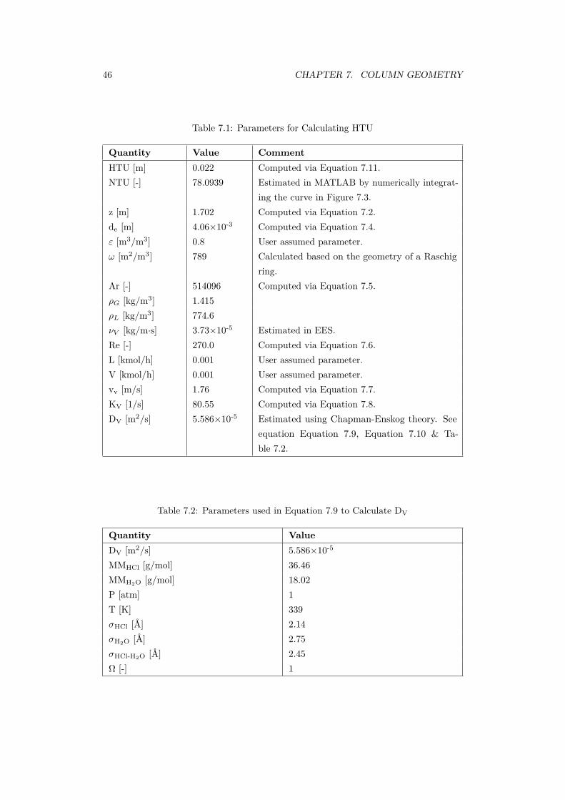
46 CHAPTER 7. COLUMN GEOMETRY
Table 7.1: Parameters for Calculating HTU
Quantity Value CommentHTU [m] 0.022 Computed via Equation 7.11.NTU [-] 78.0939 Estimated in MATLAB by numerically integrat-
ing the curve in Figure 7.3.z [m] 1.702 Computed via Equation 7.2.de [m] 4.06×10⁻³ Computed via Equation 7.4.ε [m3/m3] 0.8 User assumed parameter.ω [m2/m3] 789 Calculated based on the geometry of a Raschig
ring.Ar [-] 514096 Computed via Equation 7.5.ρG [kg/m3] 1.415ρL [kg/m3] 774.6νV [kg/m·s] 3.73×10⁻⁵ Estimated in EES.Re [-] 270.0 Computed via Equation 7.6.L [kmol/h] 0.001 User assumed parameter.V [kmol/h] 0.001 User assumed parameter.vv [m/s] 1.76 Computed via Equation 7.7.KV [1/s] 80.55 Computed via Equation 7.8.DV [m2/s] 5.586×10⁻⁵ Estimated using Chapman-Enskog theory. See
equation Equation 7.9, Equation 7.10 & Ta-ble 7.2.
Table 7.2: Parameters used in Equation 7.9 to Calculate DV
Quantity ValueDV [m2/s] 5.586×10⁻⁵
MMHCl [g/mol] 36.46MMH2O [g/mol] 18.02P [atm] 1T [K] 339σHCl [Å] 2.14σH2O [Å] 2.75σHCl-H2O [Å] 2.45Ω [-] 1

7.2. COLUMN HEIGHT 47
Table 7.3: Values used to Calculate Empirical Correlations for HETP
Quantity Value CommentρG [kg/m3] 1.415 From EES.ρL [kg/m3] 774.6 Computed in EES as weighted average by mole
fractions in the liquid phase.uG [m/s] 1.76 User assumed parameter.uL [m/s] 1 User assumed parameter.aP [m2/m3] 789 Calculated based on the geometry of a Raschig
ring.Φ [m] 0.0114 Calculated in Section 7.3.m [-] 1.13080 Constant from Table 7-2 in [52] for 1 in Pall rings,
since the table does not list Raschig rings.νL [kg/(m·s)] 3.38×10⁻⁴ Computed based on EES data @ T = 339K, P
= 101.325 kPa.σL [N/m] 0.05087 From EES.
Table 7.4: Results of Empirical Correlations for HETP
Empirical Correlation HETP [m]Ellis [49] via [34] 0.730Harrison and France [50] via [34] 0.127Kister [51] via [34] 0.229Strigle [52] via [34] 0.985Lockett [53] via [34] 0.174

48 CHAPTER 7. COLUMN GEOMETRY
The HETP correlation of Harrison and France, [50] via [34], is given by Equation 7.13.
HETP = 100ap
(7.13)
The HETP correlation of Kister, [51] via [34], is given by Equation 7.14.
HETP = 100ap
+ 0.102 (7.14)
The HETP correlation of Strigle (for 0.4 atm ≤ P ≤ 4 atm; 4mN/m ≤ σL ≤36mN/m; 0.08 cP ≤ νL ≤ 0.83 cP ), [52] via [34], is given by Equation 7.15. The symbolm represents a dimensionless constant associated with the packing, m = 1.13080 for 1 in.Pall rings (Table 7-2 in [52], Raschig rings are not listed).
HETP = exp (m − 0.187 ln (σL) + 0.213 ln (νL)) (7.15)
The HETP correlation of Lockett, [53] via [34], is given by Equation 7.16.
HETP = 1.54g0.5 (ρL − ρg)0.5 ν−0.06
ap [1 + 0.78 exp(0.00058ap)(ρg/ρL)0.25]2(7.16)
7.3 Column Diameter
An algorithm to estimate internal column diameter (Φ) is given in [47], as shown inEquations 7.17 to 7.19. Generally, a larger column diameter corresponds to a largermaximum allowable mass flow rate (of feed, distillate and bottoms). Results of thecomputation of Equations 7.17 to 7.19 are given in Table 7.5.
Φ =√
3 ·WV
π · vv(7.17)
logv2
0ωρvν0.16L
gε3(ρL − ρV ) = −0.125− 1.75(L
V
)0.25(ρV
ρL − ρV
)0.125(7.18)
vv = 0.6 · v0 (7.19)
7.4 Location of Feed Stage
The location of the feed stage (i.e., at which stage the feed is input) is determined basedon feed concentration. The feed stage is the stage (horizontal step on the “staircase”)which is above the feed concentration. The column is designed such that the feed stagecan be moved discretely along the column depending on feed concentration.

7.4. LOCATION OF FEED STAGE 49
Table 7.5: Parameters for Calculating Column Diameter
Quantity Value CommentΦ [m] 0.0114 Computed via Equation 7.17.WV [m3/s] 1.00×10⁻⁴ User assumed parameter.vv [m/s] 0.73 Computed via Equation 7.19.v0 [m/s] 1.22 Computed via Equation 7.18.ε [-] 0.8 User assumed parameter.ρL [kg/m3] 774.6 Computed in EES with T = 339 K.ρG [kg/m3] 1.415 Computed in EES with T = 339 K.ω [m2/m3] 789 Calculated based on the geometry of a Raschig
ring.νL [Pa·s] 3.38×10⁻⁴ Computed in EES with T = 339 K, P = 101.325
kPa.L [kmol/h] 0.001 User assumed parameter.V [kmol/h] 0.001 User assumed parameter.

Chapter 8
Measurement and Control
8.1 Temperature Measurement
As shown in Figure 8.1, the centerline temperatures at the zone midpoints are measuredvia T-type thermocouples, and the pipe exterior wall temperatures at the boundariesbetween zones are measured via J-type thermocouples.
Figure 8.1: Thermocouple locations and temperature zones.
50

8.2. COLUMN HEATING 51
8.2 Column Heating
The column is heated via six 125 W heating tapes (one per temperature zone, total:750 W), wrapped helically around the exterior of the column. Heat is transferred to thecolumn interior via conduction through the walls. To minimize heat loss, zones 2-5 arewrapped with fiberglass insulation. The column energy balance is as follows:
∑Ein =
∑Eout
Q+ hf = hb + hd(8.1)
The distillation involves two components; in the most general case, each componentexists in two phases, for a total of four entities: H2O(g), H2O(l), HCl(g) and HCl(aq).
The two chemical species (HCl & H2O) cannot be treated separately because HCldissolves in H2O. The thermophysical and thermochemical properties of HCl(aq) aredifferent than those of both HCl(l) and H2O(l). Therefore, the enthalpies of the feed,distillate, and bottoms streams (hf, hb, hd; respectively) are found via Chemcad’sproperty calculator. Values of h are negative due to Chemcad’s selection of the referencestate. Column heat input (Q) is calculated via Equation 8.1. It is unfeasible to performthe property calculations for hf, hb and hd in EES, as EES does not support HCl(aq).EES also returns a fatal error when a temperature argument in a property calculationexceeds a component’s critical temperature. Chemcad does not suffer these limitations.The time (t) required, per mole of feed, for the column to reach operating temperatureis calculated by Equation 8.2. The heating tapes are assumed to have 100% energyefficiency because they are ohmic (resistance) heaters. More heating tapes (larger Q)would result in a shorter heating time per mole of feed (t). Calculation results aretabulated in Table 8.1.
It is assumed that all the energy emitted from the heating tape is used to heat thecolumn. However, not all the heat from the tape goes to the column (e.g., some heatgoes to the ambient air), therefore, the heating time per mole of feed (t) is longer thanthat predicted by Equation 8.2.
t = Q
Q(8.2)
8.3 Control System
8.3.1 Schmitt Trigger
A LabView program is used to maintain column axial temperature profile. T-typethermocouples are used as analog inputs to LabView to measure temperature. The NI

52 CHAPTER 8. MEASUREMENT AND CONTROL
Table 8.1: Parameters for Calculating Column Heat Input
Quantity Value Commentxd [-] 0.99xf [-] 0.2232xb [-] 0.13Td [K] 298 Assumed, Td is near Tambient since mambient air md.Tf [K] 350Tb [K] 375hd [J/mol] -9.43×10⁴ Data from Chemcad.hf [J/mol] -2.51×10⁵ Data from Chemcad.hb [J/mol] -2.65×10⁵ Data from Chemcad.Q [J/mol] -1.08×10⁵ Calculated via Equation 8.1.Q [W] 750 Given in heating tape data.t [s/mol] 144.2 Calculated via Equation 8.2.
9472 digital output module generates a binary (on/off) control signal, according to theLabView program, which is used to switch relays. The relays, in turn, switch heatingtapes. A control diagram is shown in Figure 8.2. A Schmitt trigger is implemented inthe LabView program to prevent high-frequency oscillation of the control signal. Thethresholds of the Schmitt trigger are defined in Equations 8.3 and 8.4. A lower offsetmoves the thresholds closer together, which results in less deviation from the setpoint(i.e., less error) but increases the frequency of oscillation. A flowchart of the Schmitttrigger is shown in Figure 8.3.
The Schmitt trigger resulted in large amplitude osciallations about the setpoint. Therefore,it is abandoned in favor of proportional control.
Upper threshold = Setpoint+Offset (8.3)
Lower threshold = Setpoint−Offset (8.4)
8.3.2 PID Control
Since a Schmitt trigger is inadequate for maintaining the temperature near a setpoint,PID control (proportional, integral, differential) is used to maintain the temperatureof a zone at a setpoint with minimal fluctuation (oscillation amplitude) and minimalerror (difference between setpoint and process variable (e.g., temperature)). Error isgiven by Equation 8.5. A flowchart of PID control is given in Figure 8.4. The power of aheating tape is varied by changing the duty cycle of pulse-width modulation (PWM). A

8.3. CONTROL SYSTEM 53
Figure 8.2: Control diagram for n temperature zones.
Figure 8.3: Schmitt trigger flowchart.
PWM period of 20 seconds is selected to decrease the prevalence of rapid switching ofthe mechanical relays, which leads to their premature failure.
e(t) = r(t)− y(t) (8.5)
where:
• e(t) is the error at time t,
• r(t) is the setpoint at time t,
• y(t) is the process variable at time t (in this case, y(t) is temperature []).
PID control is described by Equation 8.6:
u(t) = kpe(t) + ki
∫ t
0e(τ) dτ + kd
de
dt(8.6)
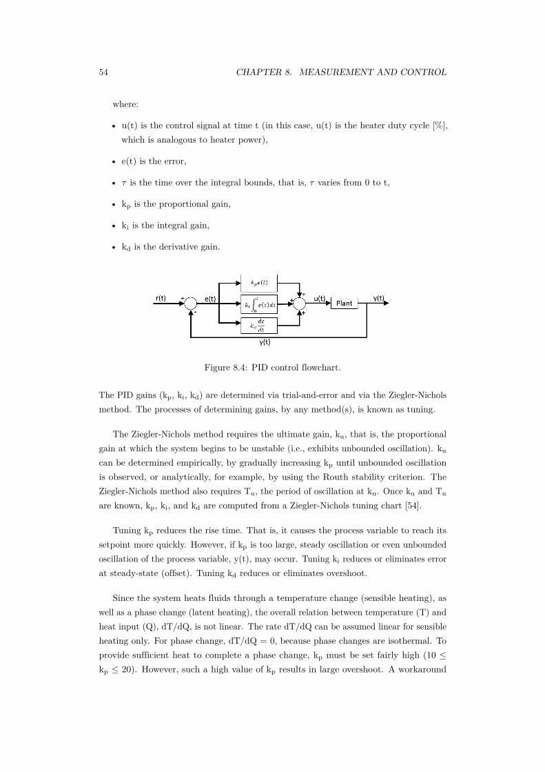
54 CHAPTER 8. MEASUREMENT AND CONTROL
where:
• u(t) is the control signal at time t (in this case, u(t) is the heater duty cycle [%],which is analogous to heater power),
• e(t) is the error,
• τ is the time over the integral bounds, that is, τ varies from 0 to t,
• kp is the proportional gain,
• ki is the integral gain,
• kd is the derivative gain.
Figure 8.4: PID control flowchart.
The PID gains (kp, ki, kd) are determined via trial-and-error and via the Ziegler-Nicholsmethod. The processes of determining gains, by any method(s), is known as tuning.
The Ziegler-Nichols method requires the ultimate gain, ku, that is, the proportionalgain at which the system begins to be unstable (i.e., exhibits unbounded oscillation). ku
can be determined empirically, by gradually increasing kp until unbounded oscillationis observed, or analytically, for example, by using the Routh stability criterion. TheZiegler-Nichols method also requires Tu, the period of oscillation at ku. Once ku and Tu
are known, kp, ki, and kd are computed from a Ziegler-Nichols tuning chart [54].
Tuning kp reduces the rise time. That is, it causes the process variable to reach itssetpoint more quickly. However, if kp is too large, steady oscillation or even unboundedoscillation of the process variable, y(t), may occur. Tuning ki reduces or eliminates errorat steady-state (offset). Tuning kd reduces or eliminates overshoot.
Since the system heats fluids through a temperature change (sensible heating), aswell as a phase change (latent heating), the overall relation between temperature (T) andheat input (Q), dT/dQ, is not linear. The rate dT/dQ can be assumed linear for sensibleheating only. For phase change, dT/dQ = 0, because phase changes are isothermal. Toprovide sufficient heat to complete a phase change, kp must be set fairly high (10 ≤kp ≤ 20). However, such a high value of kp results in large overshoot. A workaround

8.3. CONTROL SYSTEM 55
is to manually decrease kp immediately after a phase change is finished (i.e., when thetemperature begins to increase again), or shortly before a phase change is estimatedto finish. More accurate control would result if u(t), the control signal (duty cycle),is calculated based on enthalpy instead of temperature, however, there are no devicesavailable that directly measure enthalpy.
For the insulated zones (zones 2-5), kp is initially approximately 11; when thephase change (boiling) is nearly complete, kp is decreased to approximately 7. For theuninsulated zones (zones 0-1), kp is initially between 15 and 25; when the phase change(boiling) is nearly complete, kp is decreased to approximately 10. The variable kp ishigher for the uninsulated zones since a higher duty cycle is required because the rate ofheat loss is greater.
It is determined that proportional control alone is adequate for the purpose of thisresearch, therefore, ki = kd = 0. Integral control is not necessary because a few ofsteady-state error (offset) is allowable. Derivative control is also unnecessary becauseovershoot is permissible (i.e., the materials can withstand the higher temperatures thatoccur during overshoot), simply more time is required for the temperature zone to reachsteady-state.
The transfer function, H(s), of an element in a control system (e.g., controller, plant)is given by Equation 8.7.
H(s) = Y (s)X(s) (8.7)
where:
• Y(s) is the Laplace transform of the output, y(t),
• X(s) is the Laplce transform of the input, x(t).
The Laplace transform maps a function of t (time) to a function of s (complex frequency,s = σ + jω), as shown by Equation 8.8.
L f(t) = F (s) (8.8)
The input is an approximated impulse. That is, one heating tape is run at 100% dutycycle (125 W) for t ≤ 25 s, then at 0% duty cycle for t > 25 s. All other heating tapesare held constant at 0% duty cycle. This input may be considered an impulse since 25 sis negligible relative to the duration of observation (> 1 hr).
To reduce column start-up time (time required for all zones to be stabilized at theirsetpoints), it is found that the heating tapes should be started in order of decreasingtemperature (i.e., those with the hottest setpoints should be started earlier). This will

56 CHAPTER 8. MEASUREMENT AND CONTROL
minimize the overheating (when T > SP) of zones with colder setpoints. Otherwise,due to the heat transfer through adjacent zones, the zones with colder setpoints will getvastly overheated and will require much time to cool to their setpoints, thus increasingstart-up time. If the heating tapes are started in order of decreasing temperature, by thetime the hottest zones are stabilized at their setpoints, the zones with colder setpointsmay already be inadvertently heated to near (or even above) their setpoints (due to heattransfer through adjacent zones) and thus will require little to no heat from their ownheating tapes.
8.3.3 Electrical Design
As mentioned in Section 8.3, relays (AutomationDirect 781-1C-24D) are used to switchthe heating tapes. The NI 9472 digital output module (which is controlled by the LabViewprogram) drives the relay coils. The NI 9472 cannot switch the heating tapes directlybecause it is rated for a maximum of 30 VDC and 0.75 A/channel [55]. Whereas, theheating tapes require 120 VAC and 1.0 A to 5.3 A (depending on the power consumptionof the tape). Therefore, each relay is controlled by the NI 9472, which switches 24 VDC(coil side). In turn, the relays switch the heating tapes at 120 VAC (contact side). Anadvantage of using relays in this manner is that they isolate the AC & DC circuits. Forexample, if a fault, such as a current spike caused by a short, occurs in an AC circuit;the current spike would not be transmitted to the DC circuit (which includes expensiveand sensitive equipment such as the NI 9472 and NI cDAQ-9174).
A critical part of the relays are the coils, which are inductors. A flyback diode(1N4007) is installed in parallel with each relay to dissipate the voltage spike that occurswhen the relay’s coil circuit is open. When the current flows through the relay coil(closed coil circuit), the coil (an inductor) stores energy in a magnetic field. When thecoil circuit is open, the coil’s polarity is reversed and the energy that was stored in themagnetic field in the coil is released as a voltage spike, as given by Equation 8.9 [56].Since the flyback diode is present, the energy of the voltage spike is dissipated in thediode. If no flyback diode was present, the voltage spike could enter sensitive equipmentin the circuit, potentially causing damage to it. The voltage stored in an inductor isgiven as:
V = LdI
dt(8.9)
where V is voltage [V], L is inductance [H], I is current [A], and t is time [s].
Furthermore, fusible disconnect switches, comprising 10 A fuses, are installed on theAC circuits. They can be operated as regular switches; however, they also comprise afuse, which melts if the current exceeds the rating (e.g., as would occur during a short),

8.3. CONTROL SYSTEM 57
thereby interrupting the current. The fuses are separable from the disconnect switch,so only the fuse is replaced after a fault. A schematic of the electrical system used tomeasure and control column temperature is given in Figure 8.5.
Figure 8.5: Electrical control schematic.

Chapter 9
Apparatus Operation
9.1 Experimental Procedure
Connect the output ports to the output chambers via hoses. Ensure all connections areair-tight. Open output chamber valves. Close feed chamber valve.
Prepare HCl(aq) solution of desired molarity at room temperature, inside the fumehood. Always pour acid into water, thereby gradually increasing the concentrationof HCl(aq) from zero. If water is added into acid (dangerous): initially, the resultingsolution will have a high concentration of H+
(aq) & Cl-(aq) ions. Since the solution has ahigh concentration of these ions, a lot of hydration of these ions will occur. Hydration ishighly exothermic; the released heat may cause the solution to boil rapidly and splatterviolently. However, if acid is added to water (the safe method), there are initially fewH+
(aq) & Cl-(aq) ions present to undergo hydration. Much less heat is released, becausemuch less hydration occurs. The logic is thus: low ion concentration → fewer ionsavaliable for hydration → less hydration → less heat released.
Ensure feed chamber valve is closed. Open feed chamber cap, inject solution into feedchamber using syringe, close feed chamber cap. Using the LabView VI, enter proportionalgains and temperature setpoints, run VI. Allow column to reach operating temperatures.Once column has reached steady-state operating temperature(s), open feed chambervalve (leave cap closed). Close valve once chamber is empty.
Allow distillation to run. Distillation is complete when all of the feed mixture isseparated (i.e., output chambers are no longer filling). Fluid flow into the outputchambers can be seen through the semi-transparent hoses which connect the column tothe feed chambers. Once distillation is complete, close output chamber valves.
Unplug electrical controls. Stop LabView VI. Allow column to cool to a safe tem-perature before touching it. Once the column is at a safe temperature, ensure that the
58

9.1. EXPERIMENTAL PROCEDURE 59
output chamber valves are closed, disconnect the output chambers from the column,and analyze the chambers as per the procedure described in Section 6.3. Dispose ofhazardous solvents, solutions, mixtures, and reaction residues as hazardous waste. Cleanup work area and lab equipment. Any HCl(aq) spills should be cleaned promptly withabsorbent. Used absorbent should be disposed as hazardous waste.

Chapter 10
Distillation ExperimentalResults and Discussion
10.1 Analysis of the Column Outputs
Based on the calculated results (Table 10.1), the column appears to be separating themixture components as expected. That is, the distillate contains less hydrogen chloridethan the feed, and the bottoms contains more hydrogen chloride than the feed. Theconcentration of hydrogen chloride in bottoms is still less than azeotropic (0.11 molefraction of hydrogen chloride). This is expected as it is not possible to distill through theazeotrope using only simple distillation. Doing so is impossible, because at the azeotropicconcentration (0.11 mole fraction of hydrogen chloride), the concentration (i.e., molefraction) of hydrogen chloride in the liquid phase is equal to that in the vapour phase.
The results of column operation are given in Table 10.1. The approximate molarityof the feed solution, ~cfeed, is provided. However, due to slight errors in solutionpreparation, the actual mole fraction of HCl molecules in the feed, xfeed, is also calculatedand provided. For purposes of analysis, xfeed should be used instead of ~cfeed, as theformer more accurately represents the concentration of HCl molecules in the feed solution.The mole fraction of HCl in the distillate and bottoms, xcolumn output, is calculated fromρ and T using Equation 6.8. xcolumn output refers collectively to xdistillate and xbottoms.
The experiment numbers are integers assigned by the LabView program. They areincremented by +1 each time the LabView program is run. Their magnitude is arbitrary;however, they serve to identify individual experiments. The letters D and B after theexperiment numbers signify distillate and bottoms, respectively.
The distillate (D) from all experiments is calculated to have a mole fraction of HClof 0, which suggests that the distillate is virtually pure H2O(l).
60

10.1. ANALYSIS OF THE COLUMN OUTPUTS 61
Table 10.1: Measured Densities and Calculated Concentrations
ExperimentNumber
~ccolumn feed
[mol/L]xcolumn feed
[mol/mol]ρ [g/ml] xcolumn output
[mol/mol]385D 1 0.0180 0.979 0385B 1 0.0180 1.036 0.0400386D 2 0.0362 0.966 0386B 2 0.0362 1.058* 0.0655387D 1 0.0191 0.970 0387B 1 0.0191 1.091* 0.1068388D 0.5 0.0099 0.970 0388B 0.5 0.0099 1.048* 0.0547389D 3 0.0549 0.966 0389B 3 0.0549 1.072* 0.0832391D 0.5 0.0095 0.953 0391B 0.5 0.0095 1.080* 0.0944392D 2 0.0368 0.967 0392B 2 0.0368 1.076* 0.0896*Calculated after one or more filtrations. Filtration is necessary because of thecorrosion product, as described in Section 6.3.2.
The composition of the bottoms (B) from the experiments varies considerably from ex-periment to experiment. A possible reason for this variation is explained in Section 10.2.1.However, in all experiments the bottoms is calculated to have a mole fraction of HCl lessthan 0.11 (the azeotropic concentration). This is expected as it is impossible to cross theazeotrope with a single pressure; because at the azeotrope, the vapor and liquid phasesare of identical composition.
From the results given in Table 10.1, it appears that the column is separating themixture components such that:
0 ≤ xdistillate < xfeed < xbottoms < xazeotropic, where xazeotropic = 0.11 mol/mol(10.1)
This means that the column is partially separating the mixture such that the distillatehas less HCl than the feed, the bottoms has more HCl than the feed, and all threestreams (feed, bottoms, distillate) are of a concentration less than azeotropic.

62CHAPTER 10. DISTILLATION EXPERIMENTAL RESULTS AND DISCUSSION
10.1.1 Comparison of Experimental Results and Simulation Re-sults
As shown by Table 10.2, there is reasonable agreement between the experimental andsimulation results. All experiments and simulations in Table 10.2 satisfy the criterion ofEquation 10.1.
However, there are discrepancies between the experimental xoutput and the simulatedxoutput for similar feed concentrations. For example, identifier 388 and identifier 1 havesimilar feed concentrations. Yet for experimental, x bottoms 388 = 0.0547, whereas, forsimulated, xbottoms 1 = 0.03. The experimental output concentration is approximately1.8 times the simulated output concentration, despite very similar feed concentrations.This discrepancy may be due to the fact that the experimental unit is a packed columnwhereas the simulated unit is a perforated-plate column. Furthermore, the simulated unitmay be of insufficient length (i.e., not enough plates) to achieve the maximum possibledegree of separation.
10.2 Weaknesses & Limitations in the Results
10.2.1 Corrosion Product
The considerable variation in mole fraction of HCl for the bottoms is likely due to thepresence of corrosion product (Figure 6.2). The presence of corrosion product affectsthe calculation of the density, ρ, which in turn affects the determination of the molefraction of HCl in the distillate or bottoms, xoutput. Any output product, the distillate orbottoms, can only be filtered a finite number of times, as the filter absorbs some liquideach time a liquid is poured through it. Thus, the mass that leaves the filter is less thanthe mass that enters it.
10.2.2 Vapour Pressure of the Vapour Phase
It is not feasible to analyze y, the mole fraction of HCl in the vapour phase, as the vapourpressure of HCl(aq) is ≤ 0.04 kPa at the concentrations (< 7 mol/L) and temperatures(approximately 20 ) in question, according to Fritz [57]. Pressure gages of the requiredsensitivity are not available at the time of experimentation.

10.2. WEAKNESSES & LIMITATIONS IN THE RESULTS 63
Table 10.2: Comparison of Experimental Results and Simulation Results
Identifier xfeed [mol/mol] xoutput [mol/mol]
Experimental
385D 0.0180 0385B 0.0180 0.0400386D 0.0362 0386B 0.0362 0.0655387D 0.0191 0387B 0.0191 0.1068388D 0.0099 0388B 0.0099 0.0547389D 0.0549 0389B 0.0549 0.0832391D 0.0095 0391B 0.0095 0.0944392D 0.0368 0392B 0.0368 0.0896
Simulation
1D 0.01 0.001B 0.01 0.032D 0.03 0.002B 0.03 0.103D 0.05 0.033B 0.05 0.11
In the 2nd column, D and B signify distillate and bottoms, respectively.
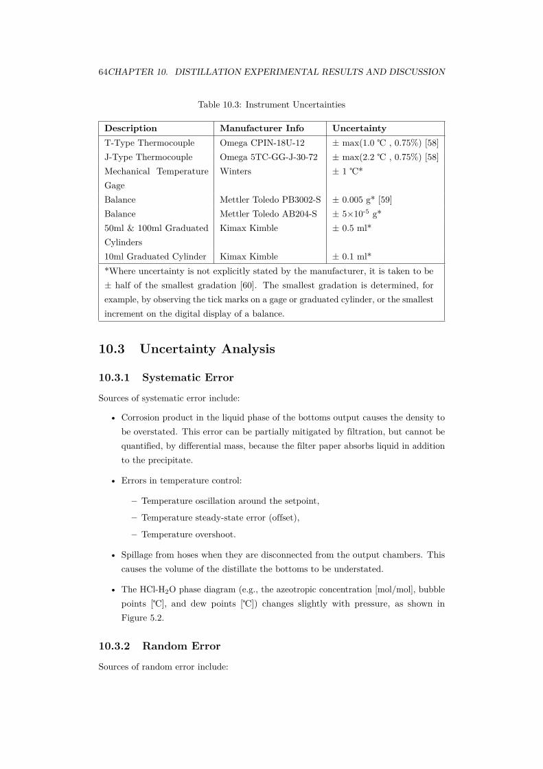
64CHAPTER 10. DISTILLATION EXPERIMENTAL RESULTS AND DISCUSSION
Table 10.3: Instrument Uncertainties
Description Manufacturer Info UncertaintyT-Type Thermocouple Omega CPIN-18U-12 ± max(1.0 , 0.75%) [58]J-Type Thermocouple Omega 5TC-GG-J-30-72 ± max(2.2 , 0.75%) [58]Mechanical TemperatureGage
Winters ± 1 *
Balance Mettler Toledo PB3002-S ± 0.005 g* [59]Balance Mettler Toledo AB204-S ± 5×10-5 g*50ml & 100ml GraduatedCylinders
Kimax Kimble ± 0.5 ml*
10ml Graduated Cylinder Kimax Kimble ± 0.1 ml**Where uncertainty is not explicitly stated by the manufacturer, it is taken to be± half of the smallest gradation [60]. The smallest gradation is determined, forexample, by observing the tick marks on a gage or graduated cylinder, or the smallestincrement on the digital display of a balance.
10.3 Uncertainty Analysis
10.3.1 Systematic Error
Sources of systematic error include:
• Corrosion product in the liquid phase of the bottoms output causes the density tobe overstated. This error can be partially mitigated by filtration, but cannot bequantified, by differential mass, because the filter paper absorbs liquid in additionto the precipitate.
• Errors in temperature control:
– Temperature oscillation around the setpoint,
– Temperature steady-state error (offset),
– Temperature overshoot.
• Spillage from hoses when they are disconnected from the output chambers. Thiscauses the volume of the distillate the bottoms to be understated.
• The HCl-H2O phase diagram (e.g., the azeotropic concentration [mol/mol], bubblepoints [], and dew points []) changes slightly with pressure, as shown inFigure 5.2.
10.3.2 Random Error
Sources of random error include:

10.3. UNCERTAINTY ANALYSIS 65
• Fluctuations in the ambient temperature of the room, which affects the heat duty.
10.3.3 Method of Kline & McClintock
The method of Kline & McClintock [61] is used to determine the uncertainty of acalculated value whose arguments are measured from physical devices. A MATLABscript, given in Appendix A.2, is written to perform the method of Kline & McClintock.
According to Kline & McClinotck [61], for a calculated result, R, which is calculatedfrom the measured independent variables, x1, x2,...,xn, then the uncertainty of thatresult, wR, is:
wR =[(
δR
δx1w1
)2+(δR
δx2w2
)2+ ...+
(δR
δxnwn
)2]1/2
(10.2)
where:
• x1, x2,...,xn are the independent variables of which R is a function, i.e., R = f(x1,x2,...,xn). The values of x1, x2,...,xn are physically measured using instruments.
• wn is the uncertainty of independent variable xn (e.g., the given uncertainty of aninstrument),
• R is the calculated result,
• wR is the uncertainty of the calculated result.
Uncertainties determined via the method of Kline & McClintock (calculated via theMATLAB script given in Appendix A.2) are given in Table 10.4. The letters D and Bafter the experiment numbers signify distillate and bottoms, respectively. Table 10.4also shows the maximum and minimum output product concentrations that occur dueto the uncertainties. These maximum and minimum output product concentrations arecalculated as:
Maximum Output Product Concentration : xoutput, max = xoutput + wxoutput(10.3)
Minimum Output Product Concentration : xoutput, min = xoutput − wxoutput (10.4)
The variables xoutput, max and xoutput, min give the maximum and minimum values ofxoutput. They are computed by Equation 10.3. The resulting range in the value xoutput
is caused by uncertainties in measurement (instrument uncertainty) and calculation.Of course, it is not possible that xoutput < 0. Whenever this occurs, xoutput should befloored to zero. As discussed earlier, it is not possible to cross the azeotrope, therefore,when xoutput > 0.11, it should be capped to 0.11.

66CHAPTER 10. DISTILLATION EXPERIMENTAL RESULTS AND DISCUSSION
Table 10.4: Uncertainties, following the approach of Kline & McClintock
ExperimentNumber
wxfeed
[mol/mol]wρ
[g/ml]wxoutput
[mol/mol]xoutput, min
[mol/mol]xoutput, max
[mol/mol]385D ±2.115×10⁻⁵ ± 0.0122 ± 0.0148 -0.0148 0.0148385B ±2.115×10⁻⁵ ± 0.0123 ± 0.0149 0.0251 0.0549386D ±2.102×10⁻⁵ ± 0.0112 ± 0.0136 -0.0136 0.0136386B ±2.102×10⁻⁵ ± 0.0132 ± 0.0160 0.0495 0.0815387D ±2.103×10⁻⁵ ± 0.0099 ± 0.0120 -0.0120 0.0120387B ±2.103×10⁻⁵ ± 0.0123 ± 0.0149 0.0919 0.1217388D ±2.116×10⁻⁵ ± 0.0110 ± 0.0133 -0.0133 0.0133388B ±2.116×10⁻⁵ ± 0.0125 ± 0.0151 0.0396 0.0698389D ±2.100×10⁻⁵ ± 0.0138 ± 0.0167 -0.0167 0.0167389B ±2.100×10⁻⁵ ± 0.0244 ± 0.0294 0.0538 0.1126391D ±2.120×10⁻⁵ ± 0.0113 ± 0.0137 -0.0137 0.0137391B ±2.120×10⁻⁵ ± 0.0124 ± 0.0150 0.0794 0.1094392D ±2.094×10⁻⁵ ± 0.0106 ± 0.0128 -0.0128 0.0128392B ±2.094×10⁻⁵ ± 0.0211 ± 0.0255 0.0641 0.1151
The uncertainties are reasonable and are small enough that mixture separation canstill be observed in most cases. That is, the relation
0 ≤ xdistillate < xfeed < xbottoms < xazeotropic, where xazeotropic = 0.11 mol/mol(10.5)
holds true for most experiments, even after allowing for the range in values caused byuncertainties. Alternatively, this can be expressed as, for most experiments:
xoutput,bottoms,max > xoutput,bottoms,min > xfeed (10.6)
andxoutput,distillate,min < xoutput,distillate,max < xfeed (10.7)
The variation (or range) in xfeed (on the order of 10-5) is negligible compared to thevariation in xoutput (on the order of 10-2). This approximately thousand-fold difference invariation is because wxfeed wxoutput . The variable wxoutput is relatively large because wρis also relatively large. The uncertainty of the calculated density, wρ, can be decreasedby using instruments of higher precision when measuring mass and volume, which areused to calculate ρ.
10.4 Distillation Conclusions and Recommendations
As shown by Table 10.1, the column separates the mixture adequately when the feedconcentration is less than azeotropic (xfeed < 0.11). Feed concentrations greater than

10.4. DISTILLATION CONCLUSIONS AND RECOMMENDATIONS 67
azeotropic (xfeed > 0.11, or cfeed > ~7.0 mol/L) are not investigated since it would causesevere corrosion to the column, possibly rendering it inoperable for future experiments.
If the feed concentration is limited to xfeed < 0.11, then no relation is found betweenxfeed and the xoutput (xoutput refers collectively to xdistillate and xbottoms). As long asxfeed is any concentration less than azeotropic (0.11 mol/mol), xdistillate tends to 0mol/mol and xbottoms tends to 0.11 mol/mol. This is reasonable because the column is ofsufficient height (see Section 7.2) to achieve the maximum possible degree of separation.The knowledge gained from the distillation experiments described in this thesis canbe presently applied to the Cu-Cl cycle, in order to concentrate and recycle HCl(aq).By recycling HCl(aq), financial savings are realized. This constitutes a step towardoptimization and integration.
To reinforce the knowledge gained by the experiments described in this thesis, it isrecommended that another column be made from materials that do not corrode in thepresence of HCl. Thus the output products (i.e., distillate and bottoms) would be freefrom corrosion and the errors caused by it. The results from the new column could becompared with the results given in this thesis, to quantify the errors caused by corrosion.
As shown in Table 10.4, the largest uncertainty occurs with concentration of the outputproduct, that is wxoutput is the largest uncertainty This, in turn, is due to the density,ρ, having a large uncertainty, wρ. Therefore, another recommendation to reinforce theknowledge gained by the experiments is to use instruments of higher precision and higherresolution when measuring the mass and volume to calculate output product density, ρ.
Furthermore, the availability and performance of various techniques (e.g., chemicalanalyzers, reagent strips) should be investigated to determine if there are feasible methodsto directly measure HCl concentration.
At the time of the experiments described in this thesis, gages of the required sensitiveare unavailable. An important future step is to use sensitive pressure gages on (i.e., therange of 0.04 kPa) to analyze the vapour phase (i.e., measure the vapour pressure) whenthe liquid phase is subcooled.
Another logical future step is to examine the heat duty to increase the energy efficiencyof the column. The focus of this research is to examine the concentrations of the output,and little attention is paid to energy efficiency. (i.e., This research is for proof-of-concept,whereas further research on this topic would be for optimization and refinement).

Chapter 11
Conclusions andRecommendations
Conclusions and recommendations relating to distillation as well as those relating to theeffect of metastability on crystallization are presented in this chapter.
HCl(aq) concentration via distillation, as well as the effect of metastability on CuCl2(aq)
recovery via crystallization, are each important steps toward the optimization andintegration of the Cu-Cl cycle. HCl(aq) concentration via distillation serves to decreasethe operating cost of the cycle, because it recycles HCl(aq). Metastability has the effectof decreasing the thermal energy requirements of the Cu-Cl cycle because it decreasesthe precipitation temperature of CuCl2(aq) from HCl(aq) solutions.
Thus the objective of demonstrating the feasibility of increasing HCl(aq) concentrationvia distillation, as described in Chapter 1, is achieved. Also, the objective of investigatingthe relationship between cooling rate and MSZW for the crystallization of CuCl2(aq)
from HCl(aq) solutions, as described in Section 4.2, is achieved.
Key findings are described as follows. The distillation system is found to separatethe mixture as expected. The concentration of hydrogen chloride in the distillate isfound to be less than that in the feed. The concentration of hydrogen chloride in thebottoms product is found to be greater than that in the feed, but less than azeotropic.However, the determination of hydrogen chloride concentration is hindered by corrosionproduct in the bottoms product. Please refer to Chapter 10 for a detailed analysis ofthe distillation results. MSZW is found to decrease with HCl(aq) concentration and toincrease with cooling rate. A larger MSZW suggests a lower precipitation temperature,resulting in thermal energy savings. Please refer to Section 4.2.3 for a detailed analysisof the metastability results.
68

69
In order to obtain a more thorough understanding of HCl(aq) distillation, which in turnwill help optimize the Cu-Cl cycle, it is recommended that further distillation experimentsbe performed at higher feed molarities. It is also recommended that corrosion ideallybe prevented from occurring in the first place (i.e., by selecting non-reactive columnmaterials), or, failing this, to more accurately determine the error in the calculation ofconcentration caused by the presence of corrosion product.
In order to obtain a more thorough understanding of the effect of metastability onthe crystallization of CuCl2(aq) from HCl(aq) solutions, it is recommended that moresophisticated methods than the unaided eye be used to detect the onset of nucleation,which is the first step of crystal formation. This will result in more accurate determinationof the precipitation temperature.

References
[1] Steam methane reforming. Student Energy. Accessed 28 June 2017. [Online].Available: https://www.studentenergy.org/topics/steam-methane-reforming
[2] G. Naterer, S. Suppiah, L. Stolberg, M. Lewis, S. Ahmed, Z. Wang, M. Rosen, I. Din-cer, K. Gabriel, E. Secnik, E. Easton, S. Lvov, V. Papangelakis, and A. Odukoya,“Progress of international program on hydrogen production with the copper-chlorinecycle,” International Journal of Hydrogen Energy, vol. 39, pp. 2431–2445, 2014.
[3] M. Fayazuddin, “Challenges associated with separation of hcl-water azeotrope incopper-chlorine thermochemical hydrogen generation cycle (a case study),” RajivGandhi Institute of Petroleum Technology, Rae Bareli, Tech. Rep., 2015.
[4] S. Aghahosseini, “System integration and optimization of copper-chlorine thermo-chemical cycle with various options for hydrogen production,” Ph.D. dissertation,University of Ontario Institute of Technology, Oshawa, Ontario, Canada, 2013.
[5] R. Li, Q. Ye, X. Suo, X. Dai, and H. Yu, “Heat-integrated pressure-swing distillationprocess for separation of a maximum-boiling azeotrope ethylenediamine/water,”Chemical Engineering Research and Design, vol. 105, pp. 1–15, 2016.
[6] Azeotrope / azeotropic mixture. Seperation Processes. Accessed 27 June 2017.[Online]. Available: http://www.separationprocesses.com/Distillation/DT_Chp01f.htm
[7] Misc distillation - azeotropic. Separation Processes. Accessed 27 June 2017. [Online].Available: http://separationprocesses.com/Distillation/DT_Chp06c07.htm
[8] J. P. Knapp and M. F. Doherty, “A new pressure-swing distillation process forseparating homogeneous azeotropic mixtures,” Ind. Eng. Chem Res., vol. 31, pp.346–357, 1992.
[9] I. Chien, K. Zeng, and H. Chao, “Design and control of a complete heterogeneousazeotropic distillation column system,” Ind. Eng. Chem. Res., vol. 43, pp. 2160–2174,2004.
70

REFERENCES 71
[10] Misc distillation - extractive. Separation Processes. Accessed 31 March 2017. [Online].Available: http://www.separationprocesses.com/Distillation/DT_Chp06d.htm
[11] Y. Wang, P. Cui, Y. Ma, and Z. Zhang, “Extractive distillation and pressure-swing distillation for thf/ethanol separation,” Journal of Chemical Technology andBiotechnology, vol. 90, no. 8, pp. 1463–1472, 2015.
[12] R. Munoz, J. Monton, M. Burguet, and J. de la Torre, “Separation of isobutylalcohol and isobutyl acetate by extractive distillation and pressure-swing distillation:Simulation and optimization,” Separation and Purification Technology, vol. 50, no. 2,pp. 175–183, 2006.
[13] E. Lladosa, J. B. Monton, and M. C. Burguet, “Separation of di-n-propyl ether andn-propyl alcohol by extractive distillation and pressure-swing distillation: Computersimulation and economic optimization,” Chemical Engineering and Processing,vol. 50, no. 11-12, pp. 1266–1274, 2011.
[14] E. Hosgor, T. Kucuk, I. N. Oksal, and D. B. Kaymak, “Design and control ofdistillation processes for methnaol-chloroform separation,” Computers and ChemicalEngineering, vol. 67, pp. 166–177, 2014.
[15] W. L. Luyben, “Comparison of extractive distillation and pressure-swing distillationfor acetone/chloroform separation,” Computers and Chemical Engineering, vol. 50,pp. 1–7, 2013.
[16] ——, “Comparison of extractive distillation and pressure-swing distillation foracetone-methanol separation,” Ind. Eng. Chem. Res., vol. 47, no. 8, pp. 2696–2707,2008.
[17] Qvf - process systems: Concentration of hydrochloric acid above the azeotropicpoint. QVF. Accessed 6 May 2016. [Online]. Available: http://www.qvf.com/qvf-process-systems/mineral-acids/concentration-of-hydrochloric-acid.html
[18] A. Palomino, D. A. Parientes, H. Gomez, and P. Paucar, “Modelling ethanol-waterpressure swing distillation in an structured packed bed column,” Rev. Per. Quim.Ing. Quim., vol. 16, no. 1, pp. 75–84, 2013.
[19] Y. Wang, Z. Zhang, D. Xu, W. Liu, and Z. Zhu, “Design and control of pressure-swing distillation for azeotropes with different types of boiling behavior at differentpressures,” Journal of Process Control, vol. 42, pp. 59–76, 2016.
[20] A. M. Fulgueras, J. Poudel, D. S. Kim, and J. Cho, “Optimization study of pressure-swing distillation for the separation process of a maximum-boiling azeotropic systemof water-ethylenediamine,” Korean Journal of Chemical Engineering, vol. 33, no. 1,pp. 46–56, 2016.

72 REFERENCES
[21] J. R. Phimister and W. D. Seider, “Semicontinuous, pressure-swing distillation,”Ind. Eng. Chem. Res., vol. 39, pp. 122–130, 2000.
[22] G. Modla and P. Lang, “Feasibility of new pressure swing batch distillation methods,”Chemical Engineering Science, vol. 63, no. 11, pp. 2856–2874, 2008.
[23] J.-U. Repke, A. Klein, D. Bogle, and G. Wozny, “Pressure swing batch distillationfor homogenous azeotropic separation,” Chemical Engineering Research and Design,vol. 85, no. 4, pp. 492–501, 2007.
[24] A. A. Kiss and Z. Olujic, “A review on process intensification in internally heat-integrated distillation columns,” Chemical Engineering and Processing, vol. 86, pp.125–144, 2014.
[25] H. Shahandeh, J. Ivakpour, and N. Kasiri, “Feasibility study of heat-integrateddistillation columns using rigorous optimization,” Energy, vol. 74, pp. 662–674, 2014.
[26] G. H. S. F. Ponce, M. M. J. C. Alves, F. R. Maciel, and M. M. R. Wolf, “Using aninternally heat-integrated distillation column for ethanol-water separation for fuelapplications,” Chemical Engineering Research and Design, vol. 95, pp. 55–63, 2015.
[27] B. Kiran and A. K. Jana, “Assessing the performance improvement of an intensifiedheat integration scheme: Reactive pressure-swing distillation,” Applied ThermalEngineering, vol. 76, pp. 509–520, 2015.
[28] J. F. Mulia-Soto and F.-T. Antonio, “Modeling, simulation and control of an inter-nally heat integrated pressure-swing distillation process for bioethanol separation,”Computers and Chemical Engineering, vol. 35, pp. 1532–1546, 2011.
[29] S. I. Abu-Eishah and W. L. Luyben, “Design and control of a two-column azeotropicdistillation system,” Ind. Eng. Chem. Process Des. Dev., vol. 24, pp. 132–140, 1985.
[30] H. Cheng and W. L. Luyben, “Heat-integrated distillation columns for ternaryseparations,” Ind. Eng. Chem. Process Des. Dev., vol. 24, pp. 707–713, 1985.
[31] B. Kiran and A. K. Jana, “A hybrid heat integration scheme for bioethanol separationthrough pressure-swing distillation route,” Separation and Purification Technology,vol. 142, pp. 307–315, 2015.
[32] J. P. Knapp, “Exploiting pressure effects in the distillation of homogeneous azeotropicmixtures,” Ph.D. dissertation, UMI, Ann Arbor, 1991.
[33] J. Lee, J. Cho, D. M. Kim, and S. Park, “Separation of tetrahydrofuran and waterusing pressure swing distillation: Modeling and optimization,” Korean Journal ofChemical Engineering, vol. 28, no. 2, pp. 1–15, 2011.

REFERENCES 73
[34] G. Q. Wang, X. G. Yuan, and K. T. Yu, “Review of mass-transfer correlations forpacked columns,” Industrial & Engineering Chemistry Research, vol. 44, no. 23, pp.8715–8729, 2005.
[35] G. M. Larin, V. V. Minin, B. V. Levin, and Y. A. Buslaev, “Complexation in theCuCl2-HCl-H2o system,” Bulletin of the Academy of Sciences of the USSR, Divisionof chemical science, vol. 38, no. 6, pp. 1111–1116, 1989.
[36] P. Barrett and B. Glennon, “Characterizing the metastable zone width and solubilitycurve using lasentec FBRM and PVM,” Chemical Engineering Research and Design,vol. 80, no. 7, pp. 799–805, 2002.
[37] W. B. Euler, L. Kirschenbaum, and B. Ruekberg, “Determination of ksp, ∆G°,∆H°, and ∆S° for the dissolution of calcium hydroxide in water a general chemistryexperiment,” Journal of Chemical Education, vol. 77, no. 8, pp. 1039–1040, 2000.
[38] X. Ni and A. Liao, “Effects of cooling rate and solution concentration on solutioncrystallization of L-glutamic acid in an oscillatory baffled crystallizer,” CrystalGrowth & Design, vol. 8, no. 8, pp. 2875–2881, 2008.
[39] J. E. Edwards, “Process modelling selection of thermodynamic methods,”P & I Design, 2 Reed Street, Gladstone Industrial Estate, Thornaby,TS17 7AF, United Kingdom., Tech. Rep., 2008. [Online]. Available: https://www.chemstations.net/content/documents/Technical_Articles/thermo.pdf
[40] S. Hsieh, “Chemical process simulation - chemcad thermodynamic,” Tech. Rep.,2008. [Online]. Available: web.thu.edu.tw/g96310005/www/6_thermo.pdf
[41] Metals and corrosion resistance. The Engineering ToolBox. Accessed4 April 2017. [Online]. Available: http://www.engineeringtoolbox.com/metal-corrosion-resistance-d_491.html
[42] “Corrosion resistance of the austentic chromium-nickel stainless steels in chemicalenvironments,” INCO: The International Nickel Company, Inc., One NewYork Plaza, New York, N.Y. 10004, Tech. Rep., 1963. [Online]. Available:www.parrinst.com/files/Parr_Stainless-Steels-Corrosion-Info.pdf
[43] T. Bell. (2017) How to calculate the rate of metal corrosion. The Balance.Accessed 8 September 2017. [Online]. Available: https://www.thebalance.com/corrosion-rate-calculator-2339697
[44] (2000) Standard pipe schedules pipe sizes chart table data. Engineers Edge.Accessed 8 September 2017. [Online]. Available: http://www.engineersedge.com/pipe_schedules.htm

74 REFERENCES
[45] “Product data sheet 316/316l stainless steel,” AK Steel Corporation, 9227Centre Pointe Drive, West Chester, OH 45069, Tech. Rep., 2007. [Online].Available: www.aksteel.com/pdf/markets_products/stainless/austenitic/316_316l_data_sheet.pdf
[46] The complete aqueous hydrochloric acid solutions density-concentrationcalculator. handymath.com. Accessed 19 June 2017. [Online]. Available:http://www.handymath.com/cgi-bin/hcltble3.cgi?submit=Entry
[47] F. Tivadar, “Packed distillation columns,” Budapest University of Technology andEconomics - Faculty of Chemical Technology and Biotechnology, 2006. [Online].Available: cuo2.kkft.bme.hu/packed.pdf
[48] E. Cussler, Diffusion: Mass Transfer in Fluid Systems, 3rd ed. New York: Cam-bridge University Press, 2007.
[49] R. Ellis, “Simple HETP calculation for distillation columns,” Chem. Eng. News,vol. 31, p. 4163, 1953.
[50] M. E. Harrison and J. J. France, “Distillation column troubleshooting - part 2:Packed columns,” Chemical Engineering, vol. 96, no. 4, p. 121, 1989.
[51] H. Z. Kister, Distillation Design. New York: McGraw-Hill, 1992.
[52] R. F. Strigle, Packed tower design and applications : random and structured packings,2nd ed. Houston: Gulf Pub. Co., Book Division, 1994.
[53] M. J. Lockett, “Easily predict structured-packing HETPs,” Chemical EngineeringProgress;, vol. 94, no. 1, p. 60, 1998.
[54] T. B. Co. Ziegler-nichols method. Michigan Technological University. Accessed 15May 2017. [Online]. Available: http://pages.mtu.edu/~tbco/cm416/zn.html
[55] Datasheet NI 9472, National Instruments, 5 2016. [Online]. Available:www.ni.com/pdf/manuals/373509b_02.pdf
[56] Inductors and calculus. All About Circuits. Accessed 23 March 2017. [Online].Available: https://www.allaboutcircuits.com/textbook/direct-current/chpt-15/inductors-and-calculus/
[57] J. J. Fritz and C. R. Fuget, “Vapor pressure of aqueous hydrogen chloride solutions,0 to 50C,” Industrial and Engineering Chemistry, vol. 1, no. 1, pp. 10–12, 1956.
[58] Wire color codes and limits of error. Omega. Accessed 24 May 2017. [Online].Available: https://www.omega.ca/techref/colorcodes.html

REFERENCES 75
[59] PB3002-S - documentation. Mettler Toledo. Accessed 24 May 2017. [Online]. Avail-able: http://www.mt.com/ca/en/home/phased_out_products/others/PB3002-S.tabs.documents.html
[60] Errors and uncertainty. Paul Nicholls. Accessed 29 June 2017. [Online]. Available:http://pfnicholls.com/physics/Uncertainty.html
[61] Uncertainty analysis. SMU Lyle School of Engineering. Accessed 17 June 2017.[Online]. Available: http://lyle.smu.edu/me/2142/uncert/uncert.htm

Appendix A
Scripts
A.1 McCabe-Thiele Method
A MATLAB script that performs the McCabe-Thiele method and also calculates NTUfor the Method of Transfer Units.
1 clear all; close all; clc;
2 % USER SET PARAMETERS
3 xb = 0.13; % Bottoms composition [mole fraction HCl]
4 xf = 0.2232; %Feed composition [mole fraction HCl]
5 xd = 0.99; % Distillate (tops) [mole fraction HCl]
6 L = 0; %Molar flow rate of reflux
7 D = 0.05; %Molar flow rate of distillate
8 q = 0.999; %Mole fraction of liquid in feed
910 x1 = 0:0.01:1;
11 data_name = ’xy_vle_100000Pa .xlsx ’;
12 y1 = transpose ( xlsread (data_name ,’E12:E112 ’)); % Import Chemcad
tabulated data from Excel
13 y = x1; % Equation of the y=x line
14 plot(x1 ,y1 ,’Color ’,’r’,’LineWidth ’ ,4) %Plot the VLE curve.
15 hold on
16 plot(x1 ,y,’Color ’ ,[0.6 0.6 0.6] , ’LineWidth ’ ,2) %Plot the y=x
line
17 axis ([0 1 0 1])
18 plot_title = title( data_name (1: end -5)); %The code (1: end -5)
extracts a substring from the string data_name by removing the
last 5 characters .
19 set(plot_title ,’interpreter ’,’none ’,’FontSize ’ ,18) % Changes the
interpreter for the string plot_title so underscores are
displayed as -is , and not as subscripts .
76

A.1. MCCABE-THIELE METHOD 77
20 xlabel (’x_1 HCl Liquid Mole Fraction [-]’,’FontSize ’ ,18)
21 ylabel (’y_1 HCl Vapor Mole Fraciton [-]’,’FontSize ’ ,18)
22 set(gca ,’TickDir ’,’both ’,’FontSize ’ ,16);
23 hold on
2425 line ([xb xb],[0 xb],’Color ’,’k’,’LineWidth ’ ,2); %Draw a line for
the bottoms composition
26 line ([xf xf],[0 xf],’Color ’,’k’,’LineWidth ’ ,2); %Draw a line for
the feed composition
27 line ([xd xd],[0 xd],’Color ’,’k’,’LineWidth ’ ,2); %Draw a line for
the distillate composition
2829 m_rec = L/(D+L); %Slope of rectifying line
30 b_rec = xd - m_rec*xd; %Y- Intercept of rectifying line
31 rec_line = @(x) m_rec*x + b_rec; % Equation of rectifying line
32 hold on
3334 m_q = q/(q -1); %Slope of q-line
35 b_q = xf - m_q*xf; %Y- Intercept of q-line
36 q_line = @(x) m_q*x + b_q; % Equation of q-line
37 hold on
3839 intersection_x = (b_q - b_rec)/( m_rec - m_q);
40 intersection_y = m_rec* intersection_x + b_rec;
4142 if isnan( intersection_x ) %Plot the rectifying line
43 fplot(rec_line ,[0 xd],’Color ’,’b’,’LineWidth ’ ,4)
44 else
45 fplot(rec_line ,[ intersection_x xd],’Color ’,’b’,’LineWidth ’ ,4)
46 end
474849 if isnan( intersection_x ) %Plot the q-line
50 fplot(q_line ,[0 xf],’Color ’ ,[1 0.6 0],’LineWidth ’ ,4)
51 else
52 fplot(q_line ,[ min( intersection_x , xf),max( intersection_x , xf)],
’Color ’ ,[1 0.6 0],’LineWidth ’ ,4)
53 end
5455 line ([xb intersection_x ],[xb intersection_y ],’Color ’,’g’,’LineWidth
’ ,4) %Draw the stripping line
5657 m_s = (xb - intersection_y )/(xb - intersection_x ); %Slope of
stripping line

78 APPENDIX A. SCRIPTS
58 b_s = xb - m_s*xb; %Y-
Intercept of stripping line
59 s_line = @(x) m_s*x + b_s; % Equation
of stripping line
60 fplot(s_line ,[0 intersection_x ]) %Plot the
stripping line
6162 % Estimating the average slope of the VLE curve by taking the
average slope
63 %of tangents at equal intervals .
6465 n = 10; % Number of slope sample points
66 mi = zeros (1,n); %Pre - allocate array to increase speed and save
memory .
6768 for j = 1:n %j is the loop index (loop counter )
69 a = int32(j*(( length (x1) -1)/n));
70 mi(j) = (y1(a+1) -y1(a))/(x1(a+1) -x1(a));
71 end
7273 mi;
74 ma = sum(mi (:))/ length (mi) % Display average slope of VLE curve.
7576 % METHOD OF TRANSFER UNITS
77 yNTU = zeros (1, int32 (100*xd -100* xb)); %Pre - allocate array to
increase speed and save memory .
7879 for j = int32 (100* xb :100* xd)
80 if j < int32 (100* intersection_x )
81 yNTU(j-int32 (100* xb)+1) = s_line (x1(j+1)); %y-
coordinate of stripping line (xb < x1 <= intersection_x )
82 elseif j >= int32 (100* intersection_x +1)
83 yNTU(j-int32 (100* xb)+1) = rec_line (x1(j+1)); %y-
coordinate of rectifying line ( intersection_x < x1 < 1)
84 end
85 end
8687 deltay_NTU = y1(int32 (100* xb):int32 (100* xd) -1) - yNTU (1: end -1);
88 figure2 = figure ; %Plot figure to a new window .
89 yb = s_line (xb);
90 yd = rec_line (xd);
91 plot(y1(int32 (100* xb):int32 (100* xd) -1) ,1./ deltay_NTU ,’LineWidth ’
,1.5)
92 % axis ([yb yd 0 80])

A.1. MCCABE-THIELE METHOD 79
93 title(’Number of Transfer Units (NTU)’,’FontSize ’ ,18)
94 xlabel (’y’,’FontSize ’ ,20)
95 ylabel (’1/(y*-y)’,’FontSize ’ ,20)
96 set(gca ,’TickDir ’,’both ’,’FontSize ’ ,20)
97 B = transpose (y1(int32 (100* xb):int32 (100* xd) -1)); % y1 represents
the y*’s
98 C = transpose (yNTU); %yNTU represents the y’s
99100 yaxis = 1./ deltay_NTU ;
101 rectangle = zeros (1, length (yaxis));
102 for j = 1: length (yaxis)
103 rectangle (j) = yaxis(j)*((yd -yb)/ length (yaxis));
104 end
105 NTU = sum( rectangle (:))

80 APPENDIX A. SCRIPTS
A.2 Method of Kline & McClintock
A MATLAB script that performs the method of Kline & McClintock.
1 clear
2 tic;
3 A = xlsread (’distillation_data .xlsx ’,’OA_2 ’,’D37:AT52 ’); % Import
data into matrix A.
45 % if (0)
6 %% 1) m_g [g]
7 syms m_full m_full_m_g
8 m_g(m_full , m_full_m_g ) = m_full - m_full_m_g ; % Define the function
m_g.
9 d0 = diff(m_g , m_full );
10 d1 = diff(m_g , m_full_m_g );
11 w_m_g = zeros(size(A ,1) ,1); % Initialize matrix , w_m_g , to store the
uncertainties for m_g.
12 w_m_full = 0.01/2; % Instrument uncertainty , given by
manufacturer .
13 w_m_full_m_g = 0.01/2; % Instrument uncertainty , given by
manufacturer .
14 for i = 1: size(A ,1)
15 m_full = A(i ,4); %Get data from matrix A.
16 m_full_m_g = A(i ,7); %Get data from matrix A.
17 %subs function allows for substitution of numerical values into
symbolic expressions .
18 w_m_g(i) = sqrt (( subs(d0)* w_m_full )^2 + (subs(d1)* w_m_full_m_g )
^2); %vpa function converts from fractional to decimal
representation .
19 end
202122 %% 2) m_empty_average [g]
23 clear d0 d1 d2 d3 % Clearing undefined variables does not
cause errors .
24 syms m_empty_1 m_empty_2 m_empty_3
25 m_empty_average (m_empty_1 ,m_empty_2 , m_empty_3 ) = ( m_empty_1 +
m_empty_2 + m_empty_3 )/3; % Define the function m_empty_average .
26 d0 = diff( m_empty_average , m_empty_1 );
27 d1 = diff( m_empty_average , m_empty_2 );
28 d2 = diff( m_empty_average , m_empty_3 );
29 w_m_empty_average = zeros(size(A ,1) ,1); % Initialize matrix ,
w_m_empty_average , to store the uncertainties for

A.2. METHOD OF KLINE & MCCLINTOCK 81
w_m_empty_average .
30 w_m_empty_1 = 0.01/2; % Instrument uncertainty ,
given by manufacturer .
31 w_m_empty_2 = 0.01/2; % Instrument uncertainty ,
given by manufacturer .
32 w_m_empty_3 = 0.01/2; % Instrument uncertainty ,
given by manufacturer .
33 for i = 1: size(A ,1)
34 m_empty_1 = A(i ,1); %Get data from matrix A.
35 m_empty_2 = A(i ,2); %Get data from matrix A.
36 m_empty_3 = A(i ,3); %Get data from matrix A.
37 w_m_empty_average (i) = sqrt (( subs(d0)* w_m_empty_1 )^2 + (subs(d1
)* w_m_empty_2 )^2 + (subs(d2)* w_m_empty_3 )^2); %vpa function
converts from fractional to decimal representation .
38 end
39404142 %% 3) m_12MHCl [g]
43 clear d0 d1 d2 d3 % Clearing undefined variables does not
cause errors .
44 syms m_H2O m_H2O_m_12MHCl
45 m_12MHCl (m_H2O , m_H2O_m_12MHCl ) = m_H2O_m_12MHCl - m_H2O; % Define
the function , m_12MHCl , by which the variable in question in
calculated .
46 d0 = diff(m_12MHCl ,m_H2O);
47 d1 = diff(m_12MHCl , m_H2O_m_12MHCl );
48 w_m_12MHCl = zeros(size(A ,1) ,1); % Define a matrix to store
the uncertainties for the variable in question .
49 w_m_H2O = 0.01/2; % Instrument uncertainty ,
given by manufacturer .
50 w_m_H2O_m_12MHCl = 0.01/2; % Instrument uncertainty ,
given by manufacturer .
51 for i = 1: size(A ,1)
52 m_H2O = A(i ,5); %Get data from matrix A.
53 m_H2O_m_12MHCl = A(i ,6); %Get data from matrix A.
54 w_m_12MHCl (i) = sqrt (( subs(d0)* w_m_H2O )^2 + (subs(d1)*
w_m_H2O_m_12MHCl )^2); %vpa function converts from
fractional to decimal representation .
55 end
565758 %% 4) v_12MHCl [ml]

82 APPENDIX A. SCRIPTS
59 clear d0 d1 d2 d3 % Clearing undefined variables does not
cause errors .
60 syms m_12MHCl
61 v_12MHCl ( m_12MHCl ) = m_12MHCl /1.19; % Define the function (i.e.,
R) by which the variable in question in calculated .
62 d0 = diff(v_12MHCl , m_12MHCl );
63 w_v_12MHCl = zeros(size(A ,1) ,1); % Define a matrix to store
the uncertainties for the variable in question .
64 for i = 1: size(A ,1)
65 m_12MHCl = A(i ,7); %Get data from matrix A.
66 w_v_12MHCl (i) = sqrt (( subs(d0)* w_m_12MHCl (i))^2); %vpa function
converts from fractional to decimal representation .
67 end
686970 %% 5) n_HClfeed [mol]
71 clear d0 d1 d2 d3 % Clearing undefined variables does not
cause errors .
72 syms v_12MHCl
73 n_HClfeed ( v_12MHCl ) = 12* v_12MHCl /1000; % Define the function (i
.e., R) by which the variable in question in calculated .
74 d0 = diff(n_HClfeed , v_12MHCl );
75 w_n_HClfeed = zeros(size(A ,1) ,1); % Define a matrix to store
the uncertainties for the variable in question .
76 for i = 1: size(A ,1)
77 v_12MHCl = A(i ,8); %Get data from matrix A.
78 w_n_HClfeed (i) = sqrt (( subs(d0)* w_v_12MHCl (i))^2); %vpa
function converts from fractional to decimal representation
.
79 end
808182 %% 6) m_HClfeed [g]
83 clear d0 d1 d2 d3 % Clearing undefined variables does not
cause errors .
84 syms n_HClfeed
85 m_HClfeed ( n_HClfeed ) = 36.46* n_HClfeed ; % Define the function (i
.e., R) by which the variable in question in calculated .
86 d0 = diff(m_HClfeed , n_HClfeed );
87 w_m_HClfeed = zeros(size(A ,1) ,1); % Define a matrix to store
the uncertainties for the variable in question .
88 for i = 1: size(A ,1)
89 n_HClfeed = A(i ,9); %Get data from matrix A.

A.2. METHOD OF KLINE & MCCLINTOCK 83
90 w_m_HClfeed (i) = sqrt (( subs(d0)* w_n_HClfeed (i))^2); %vpa
function converts from fractional to decimal representation
.
91 end
929394 %% 7) m_H2Ofeed [g]
95 clear d0 d1 d2 d3 % Clearing undefined variables does not
cause errors .
96 syms m_H2O_m_12MHCl m_HClfeed
97 m_H2Ofeed ( m_H2O_m_12MHCl , m_HClfeed ) = m_H2O_m_12MHCl - m_HClfeed ;
% Define the function (i.e., R) by which the variable in
question in calculated .
98 d0 = diff(m_H2Ofeed , m_H2O_m_12MHCl );
99 d1 = diff(m_H2Ofeed , m_HClfeed );
100 w_m_H2Ofeed = zeros(size(A ,1) ,1); % Define a matrix to store
the uncertainties for the variable in question .
101 for i = 1: size(A ,1)
102 m_H2O_m_12MHCl = A(i ,6); %Get data from matrix A.
103 m_HClfeed = A(i ,10); %Get data from matrix A.
104 w_m_H2Ofeed (i) = sqrt (( subs(d0)* w_m_H2O_m_12MHCl )^2 + (subs(d1)
* w_m_HClfeed (i))^2); %vpa function converts from fractional
to decimal representation .
105 end
106107108 %% 8) n_H2Ofeed [mol]
109 clear d0 d1 d2 d3 % Clearing undefined variables does not
cause errors .
110 syms m_H2Ofeed
111 n_H2Ofeed ( m_H2Ofeed ) = m_H2Ofeed /18.02; % Define the function (i
.e., R) by which the variable in question in calculated .
112 d0 = diff(n_H2Ofeed , m_H2Ofeed );
113 w_n_H2Ofeed = zeros(size(A ,1) ,1); % Define a matrix to store
the uncertainties for the variable in question .
114 % m_H2Ofeed = A(: ,11);
115 for i = 1: size(A ,1)
116 m_H2Ofeed = A(i ,11); %Get data from matrix A.
117 w_n_H2Ofeed (i) = sqrt (( subs(d0)* w_m_H2Ofeed (i))^2); %vpa
function converts from fractional to decimal representation
.
118 end
119120

84 APPENDIX A. SCRIPTS
121 %% 9) x_feed [mol/mol]
122 clear d0 d1 d2 d3 % Clearing undefined variables does not
cause errors .
123 syms n_HClfeed n_H2Ofeed
124 x_feed (n_HClfeed , n_H2Ofeed ) = n_HClfeed /( n_HClfeed + n_H2Ofeed );
% Define the function (i.e., R) by which the variable in
question in calculated .
125 d0 = diff(x_feed , n_HClfeed );
126 d1 = diff(x_feed , n_H2Ofeed );
127 w_x_feed = zeros(size(A ,1) ,1); % Define a matrix to store the
uncertainties for the variable in question .
128 for i = 1: size(A ,1)
129 n_HClfeed = A(i ,9); %Get data from matrix A.
130 n_H2Ofeed = A(i ,12); %Get data from matrix A.
131 if ( n_H2Ofeed ~= 0)
132 w_x_feed (i) = sqrt (( subs(d0)* w_n_HClfeed (i))^2 + (subs(d1)*
w_n_H2Ofeed (i))^2); %vpa function converts from
fractional to decimal representation .
133 end
134 end
135136137 %% 10) rho [g/ml]
138 clear d0 d1 d2 d3 % Clearing undefined variables does not
cause errors .
139 syms m_sample v_sample
140 rho(m_sample , v_sample ) = m_sample / v_sample ; % Define the
function (i.e., R) by which the variable in question in
calculated .
141 d0 = diff(rho , m_sample );
142 d1 = diff(rho , v_sample );
143 w_rho = zeros(size(A ,1) ,1); % Define a matrix to store the
uncertainties for the variable in question .
144 % m_H2Ofeed = A(: ,11);
145 w_m_sample = 0.0001/2; % Instrument uncertainty , given by
manufacturer .
146 w_v_sample = 0.2/2; % Instrument uncertainty , given by
manufacturer .
147 for i = 1: size(A ,1)
148 m_sample = A(i ,32); %Get data from matrix A for
subbing into the partial derviatives .
149 v_sample = A(i ,33); %Get data from matrix A for
subbing into the partial derviatives .
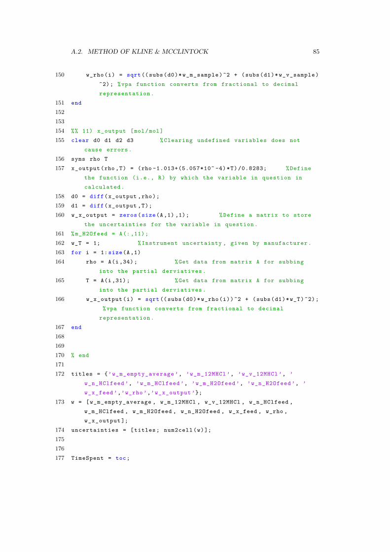
A.2. METHOD OF KLINE & MCCLINTOCK 85
150 w_rho(i) = sqrt (( subs(d0)* w_m_sample )^2 + (subs(d1)* w_v_sample )
^2); %vpa function converts from fractional to decimal
representation .
151 end
152153154 %% 11) x_output [mol/mol]
155 clear d0 d1 d2 d3 % Clearing undefined variables does not
cause errors .
156 syms rho T
157 x_output (rho ,T) = (rho -1.013+(5.057*10^ -4) *T) /0.8283; % Define
the function (i.e., R) by which the variable in question in
calculated .
158 d0 = diff(x_output ,rho);
159 d1 = diff(x_output ,T);
160 w_x_output = zeros(size(A ,1) ,1); % Define a matrix to store
the uncertainties for the variable in question .
161 % m_H2Ofeed = A(: ,11);
162 w_T = 1; % Instrument uncertainty , given by manufacturer .
163 for i = 1: size(A ,1)
164 rho = A(i ,34); %Get data from matrix A for subbing
into the partial derviatives .
165 T = A(i ,31); %Get data from matrix A for subbing
into the partial derviatives .
166 w_x_output (i) = sqrt (( subs(d0)*w_rho(i))^2 + (subs(d1)*w_T)^2);
%vpa function converts from fractional to decimal
representation .
167 end
168169170 % end
171172 titles = ’w_m_empty_average ’, ’w_m_12MHCl ’, ’w_v_12MHCl ’, ’
w_n_HClfeed ’, ’w_m_HClfeed ’, ’w_m_H2Ofeed ’, ’w_n_H2Ofeed ’, ’
w_x_feed ’,’w_rho ’,’w_x_output ’;
173 w = [ w_m_empty_average , w_m_12MHCl , w_v_12MHCl , w_n_HClfeed ,
w_m_HClfeed , w_m_H2Ofeed , w_n_H2Ofeed , w_x_feed , w_rho ,
w_x_output ];
174 uncertainties = [ titles ; num2cell (w)];
175176177 TimeSpent = toc;

Appendix B
Crystallization Results
Experiments are performed in which heated solutions of CuCl2 dissolved in variousmolarities of HCl(aq) are prepared and cooled through a temperature range. Table B.1summarizes the results of these experiments (i.e., whether or not crystals were formed).
Table B.1: Crystallization Results
mCuCl2 [g] HCl(aq)
Conc.[mol/L]
Range [] Result
45.4 6 60-20 Successful - Crystallization occurred33.5 7 20-0 Successful - Crystallization occurred19.4 9 20-0 Successful - Crystallization occurred58.3 3 20-0 Successful - Crystallization occurred
(also paste formed)38.0 7 60-20 Successful - Crystallization occurred32.1 7 20-0 Paste formed38.2 7 60-20 Successful - Crystallization occurred
(also paste formed)45.4 6 60-20 Successful - Crystallization occurred29.8 8 60-20 Successful - Crystallization occurred25.2 8 20-0 Successful - Crystallization occurred22.6 7 60-20 No stirring while pouring HCl or after
Solids in bottom of reactor (i.e., 2insoluble components (solid at bottom,liquid above)) WG13 contains liquidpipetted from top portion of reactor,Remained as the aforementioned 2phases, Oven @ 80
86

87
22.7 9 60-20 FAILED - paste formed Did not get toadd HCl(aq)
23.0 9 60-20 FAILED - Too much CuCl2 added toliquid water, Precipitate formed, Didnot get to add HCl(aq)
19.0 9 20-0 Insoluble precipitate first observed atapproximately 5near reactor bottom,Re-dissolved upon re-heating
40.3 12 20-0 FAILED - Did not crystallize,Remained liquid, Temperaturedecreased as low as 1
38.9 6 20-0 Success - Semi-crystalline pasteformed after adding HCl, No stirringwhile pouring HCl or after
38.5 6 20-0 FAILED - paste formed23.0 9 60-20 Stayed liquid, did not crystallize40.0 3 20-0 FAILED - Did not crystallize30.0 3 20-0 FAILED - Did not crystallize46.8 6 60-20 FAILED - Did not crystallize39.8 6 60-20 FAILED - paste formed39.8 6 60-20 Successful - Crystallization occurred50.2 3 20-0 Successful - Crystallization occurred54.6 3 60-20 Successful - Crystallization occurred60.28 3 60-20 FAILED - Did not crystallize67.3 3 60-20 FAILED - Did not crystallize79.8 3 20-0 FAILED - Did not crystallize, Paste
formed80.0 0 20-0 FAILED - Did not crystallize57.6 0 20-0 FAILED - Did not crystallize80.0 0 20-0 FAILED - Did not crystallize60.78 3 20-0 FAILED - Did not crystallize60.78 3 20-0 FAILED - Did not crystallize