exercise 6: single season occupancy mixture models
48
Exercises in Occupancy Estimation and Modeling; Donovan and Hines 2007 Chapter 6 Page 1 5/8/2007 EXERCISE 6: SINGLE SEASON OCCUPANCY MIXTURE MODELS Please cite this work as: Donovan, T. M. and J. Hines. 2007. Exercises in occupancy modeling and estimation. <http://www.uvm.edu/envnr/vtcfwru/spreadsheets/occupancy.htm >
-
Upload
khangminh22 -
Category
Documents
-
view
3 -
download
0
Transcript of exercise 6: single season occupancy mixture models

Exercises in Occupancy Estimation and Modeling; Donovan and Hines 2007
Chapter 6 Page 1 5/8/2007
EXERCISE 6: SINGLE SEASON OCCUPANCY MIXTURE MODELS
Please cite this work as: Donovan, T. M. and J. Hines. 2007. Exercises in occupancy modeling and estimation.
<http://www.uvm.edu/envnr/vtcfwru/spreadsheets/occupancy.htm>

Exercises in Occupancy Estimation and Modeling; Donovan and Hines 2007
Chapter 6 Page 2 5/8/2007
TABLE OF CONTENTS
SINGLE-SPECIES, SINGLE-SEASON MIXTURE MODELS SPREADSHEET EXERCISE ....................................................................................................................................3
OBJECTIVES: ........................................................................................................................3 BASIC INFORMATION ......................................................................................................3 BACKGROUND.........................................................................................................................3 MODEL PARAMETERIZATION AND OVERPARAMETERIZATION......................8 ENCOUNTER HISTORIES ............................................................................................... 10 TWO-GROUP OCCUPANCY MIXTURE MODEL SPREADSHEET INPUTS ........ 12 MULTINOMIAL LOGIT LINK ......................................................................................... 15 SPREADSHEET HISTORY PROBABILITIES .............................................................. 16 THE MIXTURE MODEL MULTINOMIAL LOG LIKELIHOOD............................... 17 MAXIMIZING THE LOG LIKELIHOOD....................................................................... 18 MIXTURE MODEL OUTPUT............................................................................................. 19 MODEL P(.)PSI FOR TWO GROUPS............................................................................ 22 MODEL P(t)PSI (ONE GROUP)....................................................................................... 26 MODEL P(.)PSI (ONE GROUP)....................................................................................... 29 SIMULATING TWO GROUP MIXTURE DATA ........................................................ 32
SINGLE SEASON OCCUPANCY MODELS ANALYSIS IN PRESENCE ................. 37 OBJECTIVES ....................................................................................................................... 37 GETTING STARTED.......................................................................................................... 37 MODEL P(t)PSI FOR TWO GROUPS............................................................................ 40 MODEL P(.)PSI FOR TWO GROUPS............................................................................ 43 MODEL P(t)PSI (ONE GROUP)....................................................................................... 45 MODEL P(.)PSI (ONE GROUP)....................................................................................... 47

Exercises in Occupancy Estimation and Modeling; Donovan and Hines 2007
Chapter 6 Page 3 5/8/2007
SINGLE-SPECIES, SINGLE-SEASON MIXTURE MODELS SPREADSHEET
EXERCISE
OBJECTIVES:
• To learn and understand the single-season two-group mixture model, and how
it fits into a multinomial maximum likelihood analysis.
• To use Solver to find the maximum likelihood estimates for the probability
of group membership, and the probability of detection and site occupancy
for each group.
• To assess the -2LogeL of the saturated model.
• To introduce concepts of model fit.
• To learn how to simulate single-season occupancy mixture data.
BASIC INFORMATION
Now that you have a solid handle on single-season occupancy modeling with both
site and survey level covariates, you’re ready to learn a few interesting spin-offs
of the basic model. In this exercise, we describe mixture models, which are
described in Chapter 5 of the book, “Occupancy Estimation and Modeling” (section
5.1). Click on the worksheet labeled “Mixtures” and we’ll get started.
BACKGROUND
The idea behind mixture models, also called heterogeneity models, is that sites in
the study area are unique in some way, such that there is heterogeneity among
sites in terms of detection and occupancy probability. In previous exercises, we
explored how to use covariates to handle individual differences among sites. For
example, we modeled occupancy as a function of habitat type and patch size, and

Exercises in Occupancy Estimation and Modeling; Donovan and Hines 2007
Chapter 6 Page 4 5/8/2007
we modeled p as a function of precipitation. In these cases, site to site
differences are handled by including covariates in the modeling process. Mixture
models, in contrast, deal with unobservable differences among sites.
Before describing the concept of unobservable heterogeneity among sites, let’s
first reinforce the concept of observable heterogeneity. Observable
heterogeneity refers to situations when the factors causing the differences can
be identified.
Example 1: Let’s assume we are surveying a collection of sites for the
occupancy of a small passerine bird. Each of the study sites has a different
detection probability that is related to patch size: the larger the patch
size, the lower the detection probability. The difference in detection
probability may occur because males might be less likely to be paired in small
patches if the small patches are lower in quality, and unmated males may sing
more often to attract a mate, hence increasing the detection probability of
the species at the site. If we can determine the patch size of each site,
then we can treat this situation by analyzing patch as a covariate for p in the
Design Matrix in MARK or PRESENCE. The data from just 5 study sites
might look like this:
Site Patch Size p 1 0.1625369 0.583574 2 0.8273964 0.418874 3 -1.940898 0.919893 4 -0.7114 0.770547 5 -1.821647 0.910654

Exercises in Occupancy Estimation and Modeling; Donovan and Hines 2007
Chapter 6 Page 5 5/8/2007
You run models where detection probabilities are constrained to be a
function of a site’s patch size, and then compare the results to models
where detection probabilities are not constrained. Using AICc methods, you
can decide if a model that includes the covariate patch size is better
supported by the data. So, with this example, the covariate patch size
allows a unique estimate of detection probability for each site, and this
covariate might account for potential differences in detection probabilities.
Example 2: Detection of sites is a function of habitat because habitats vary
in the density of a species of interest (some habitats have low densities,
while others have high densities). If the probability of detecting a species
of interest increases as population density increases (a reasonable
assumption in most cases), then the covariate “habitat type” could be
included in the p side of an occupancy model.
Both of these examples describe observable heterogeneity, and you’ve had some
practice with covariate modeling in previous exercises.
Unobservable heterogeneity, in contrast, refers to situations when the factors
causing differences in either occupancy probability or detection probability cannot
be readily identified. This could simply mean we have absolutely no clue what might
cause differences, but are willing to accept that there might be differences that
we cannot measure. For instance, if food resources are a critical predictor of
occupancy but cannot be measured readily across sites, it might impose
heterogeneity among the study sites, where some sites are rich in food resources
and others are poor, even though food was not measured directly. This

Exercises in Occupancy Estimation and Modeling; Donovan and Hines 2007
Chapter 6 Page 6 5/8/2007
unobservable heterogeneity is the focus of this exercise. A key concept in
heterogeneity models is that there may be a number of possible values for the
detection probability at each site, and the likely value for a particular site is NOT
know a priori. Heterogeneity models are well described for estimating animal
abundance with closed capture methods (see Williams et al. 2001 for a description
of the various estimators); MacKenzie et al. extend these ideas into the arena of
occupancy modeling (section 5.1)
So, how does one model unobservable heterogeneity? Well, the basic idea is that
the study sites can be divided into multiple groups, and each group (not each site)
has unique detection probabilities and a unique probability of occupancy. The
number of groups can be either a discrete number (e.g., 2 groups, 3 groups, etc.) or
an infinite number, in which the probability of being in a particular group can be
thought of as a random effect drawn from some statistical distribution. In this
exercise, we will focus on a heterogeneity model in which the group number is
discrete (n = 2), and heterogeneity is modeled for detection probability only.
Let’s assume that we are conducting a survey of 250 sites for a songbird of
interest, and that most of our observations come from the detection of singing
males. Each site is surveyed 4 times under the assumption that the population is
closed to changes in occupancy status, and with no errors in species identification.
Let’s assume that the sites differ in quality, so that fewer or no birds occur in the
low quality sites than on the high quality sites. On high-quality sites where density
is high, birds are readily detected because many birds sing during the 10 minute
survey period. On low-quality sites where the population density is low, the species
is harder to detect because very few animals occur on the site. Let’s further

Exercises in Occupancy Estimation and Modeling; Donovan and Hines 2007
Chapter 6 Page 7 5/8/2007
assume that the surveys are “rapid assessments” – meaning that sites are surveyed
for some minimal amount of time so that all 250 sites can be studied. Thus,
observers simply survey the sites quickly and do not have time to collect more
detailed data, such as metrics that might describe habitat quality (a common
design for large-scale surveys…..we’ll cover study designs in a later chapter). In
this example, we have two kinds of sites in the population: high quality sites that
have many animals and high detection probability, and low quality sites that have
few individuals and low detection probability. At any given site, the investigator
does not know the group membership.
Field biologists conduct 4 surveys on all 250 sites, and no covariates are measured.
Thus, there are 24 = 16 possible encounter histories for the study: 1111, 1110, 1101,
1100, 1011, 1010, 1001, 1000, 0111, 0110, 0101, 0100, 0011, 0010, 0001, and 0000,
and the frequency of each history is recorded.
Now, after all that work, we suspect that our sites differ in detection probability
and occupancy probability, but we have no covariates to work with in the analysis.
Now what? We could model our field data using a two-point mixture model (or two-
group heterogeneity model). You can also run three-point mixtures, four-point
mixtures, and so on. When analyzing real data, you would want to evaluate
different numbers of mixtures (including 1) and see which mixture is best
supported by the data. In this exercise, we’ll compare two-group mixture models
with one-group mixture models.

Exercises in Occupancy Estimation and Modeling; Donovan and Hines 2007
Chapter 6 Page 8 5/8/2007
Let’s look at this in more detail. We said above that
when using mixture models we divide the study sites
into groups. So, for the two-point mixture model we
divide the study sites into two groups. The population
of study sites (Ntotal) is divided into group 1 and group 2 such that Ntotal = N1 + N2,
where N1 is the total number of sites in group 1, and N2 is the total number of sites
in group 2. The first trick is to figure out the proportion of sites that belong to
group 1 and the proportion of sites that belong to group 2. We let π represent the
proportion of sites in group 1, so by definition N1 = πNtotal. Because there are only
two groups being considered, if we know N1 then we can derive N2 as
N2 = (1 – π) Ntotal because a site must be in group 2 if it wasn’t in group 1. After we
estimate the proportion of the population in each group (π and 1-π), the next step
is to estimate the detection and occupancy probabilities for each group separately.
Group 1: proportion of sites in group 1 = πNtotal, and we estimate detection
parameters p1, p2, p3, p4 and the occupancy parameter ψ specific to group 1.
Group 2: proportion of sites in group 1 = (1-π)Ntotal, and we estimate detection
parameters, p1, p2, p3, p4 and the occupancy parameter ψ specific to group 2. (Note:
as you’ll soon see, we really can’t estimate a unique ψ for group 2)
MODEL PARAMETERIZATION AND OVERPARAMETERIZATION
The first thing you need to know about mixture models is that they are very data
hungry. Because each group can have its own unique parameters, we are estimating
up to twice as many parameters than in the 1 group, single season mixture model.
Therefore, care must be taken to not over-parameterize a model. What is an
Ntotal
N2N1
π 1-π
Ntotal
N2N1
π 1-π
Ntotal
N2N1
π 1-π

Exercises in Occupancy Estimation and Modeling; Donovan and Hines 2007
Chapter 6 Page 9 5/8/2007
overparameterized model? Well, a model is overparameterized if the number of
occupancy parameters to be estimated is greater than or equal to the number of
unique encounter histories. A model that is overparameterized may not be
identifiable – that is, it might have more than one solution. Clearly, you want to
avoid this.
An example might make this more clear. Suppose you conduct a single-season
survey with three different survey periods. In this case, there are 23 = 8 possible
encounter histories. By our definition of overparameterization –- a model is
overparameterized if the number of parameters estimated is greater than or equal
to the number of unique histories -- you can run a model that estimates 7
parameters at most. If you run a two-point mixture analysis, and attempt to
estimate π, in addition to ψ, p1, p2, and p3 for each group, you will be estimating 9
total parameters. Whoops! This model MIGHT run, and MIGHT even give you
parameter estimates, but the estimates would not be valid. In other words, it’s up
to you to determine if the model is overparameterized or not.
Now, what if we surveyed the sites 4 times instead of 3 times? There would be 24
= 16 types of encounter histories, and thus you can run a model with 15 or fewer
occupancy parameters. Now, if you run this model for two groups, you would
estimate π, ψ1, p1,1, p2,1, p3,1, p4,1, ψ2, p1,2, p2,2, p3,2, p4,2 – which is a total of 11
parameters. Thus, the model degrees of freedom would be 16 (the number of
unique histories from the saturated model) minus 11 (from the occupancy model) =
5, so you haven’t overparameterized this model. HOWEVER, and this is important,
you must constrain ψ1 = ψ2 or the model is not identifiable. With that additional
constraint, you would be estimating 10 total parameters. The take-home message

Exercises in Occupancy Estimation and Modeling; Donovan and Hines 2007
Chapter 6 Page 10 5/8/2007
is that if you want to estimate time-specific p's in the mixture model, you'll need
at least 4 occasions (16 possible histories).
ENCOUNTER HISTORIES
Although there are a lot more parameters to consider, the encounter history
probabilities are a simple extension of what we did for the single-season, single-
species exercise – the only addition is the group membership identification (π) or
(1-π), and the group-specific detection and occupancy parameters. Because the
detection parameters are group specific, we need to add some notation for a two-
point mixture. Let detection probabilities be denoted as pij, where i denotes the
occasion and j denotes the group. For example, p11 is the probability of detection
for the first survey in a site in the first mixture and p12 is the probability of
detection for the first survey for a site in the second mixture. So the second
number that is subscripted identifies the group.
Let’s start by writing out the 1111 encounter history probability for a single-
season, single-species, 1 group model:
Probability of 1111 = ψ p1 p2 p3 p4. Right?
OK, now let’s extend this to a two-group mixture:
Probability of 1111 = π ψ1 p1,1 p2,1 p3,1 p4,1 + (1-π) ψ2 p1,2 p2,2 p3,2 p4,2
In other words, the probability of obtaining a 1111 history is the sum of two
probability terms, one for group 1 and the second for group 2. The probability of
getting a 1111 history for group 1 is π ψ1 p1,1 p2,1 p3,1 p4,1. The site must first be part
of group 1 (π), the site must be occupied (ψ1), the species must be detected on the

Exercises in Occupancy Estimation and Modeling; Donovan and Hines 2007
Chapter 6 Page 11 5/8/2007
first survey (p1,1), the species must be detected on the second survey (p2,1), the
species must be detected on the third survey (p3,1), and the species must be
detected on the fourth survey (p4,1). All of these terms are multiplied together
because all of them must occur to generate a 1111 history for a site in group 1. The
probability of getting a 1111 history for group 2 is (1-π) ψ2 p1,2 p2,2 p3,2 p4,2. The site
must first be part of group 2 (1-π), the site must be occupied (ψ2), the species
must be detected on the first survey (p1,2), the species must be detected on the
second survey (p2,2), the species must be detected on the third survey (p3,2), and
the species must be detected on the fourth survey (p4,2). All of these terms are
multiplied together because all of them must occur to generate a 1111 history for a
site in group 2. The two terms are added together because a site can be in either
group 1 (in which case the parameters apply to group 1) OR it can be in group 2 (in
which case the occupancy parameters apply to group 2).
Let’s try another history, 0101. We know that ψ1 must be equal to ψ2, so we can
drop the subscripts for ψ. In a one-group, single season model, the probability is
ψ (1-p1) p2 (1-p3) p4. We know the site was occupied because the species was
detected at least once (ψ), and we know that it was detected on surveys two (p2)
and four (p4) but not on surveys one (1-p1) or three (1-p3). If we extend this to a
two-group mixture model, the probability of a 0101 is:
π ψ (1-p1,1) p2,1 (1-p3,1) p4,1 + (1-π) ψ (1-p1,2) p2,2 (1-p3,2) p4,2.
Remember that the second subscript of a particular parameter (p1,1) defines the
group membership.
OK, let’s go through just one more, 0000. In a one-group, single season model, the
probability is ψ (1-p1) (1-p2) (1-p3) (1-p4)+(1-ψ). The site could have been occupied

Exercises in Occupancy Estimation and Modeling; Donovan and Hines 2007
Chapter 6 Page 12 5/8/2007
but missed on all four surveys, OR it could have been unoccupied. Extending this to
two group mixture model, the probability of a 0000 history would have four terms,
the first two apply to sites in group 1, while the last two apply to sites in group 2:
π ψ (1-p1,1) (1-p2,1) (1-p3,1) (1-p4,1) + π (1-ψ) + (1-π) ψ (1-p1,2) (1-p2,2) (1-p3,2) (1-p4,2) + (1-
π) (1-ψ). Make sense? Don’t forget that you have to distribute the π or (1-π)
terms for both options (the site is occupied but not detected, or the site is not
occupied).
Let’s see what happens if you let π equal 1. The probability statement for the 1111
encounter history becomes:
p(1111) = (1) ψ p1,1 p2,1 p3,1 p4,1+ (1 – 1) ψ2 p1,2 p2,2 p3,2 p4,2
or
p(1111) = (1) ψ p1,1 p2,1 p3,1 p4,1
which should look very familiar by now. So, when you ran the basic single-species,
single season occupancy model with no covariates in exercise 3, you ran a “mixture”
model in which there was only one group. Hopefully, the structure of the model is
making sense to you. Spend some time working through the other histories before
working on the spreadsheet.
TWO-GROUP OCCUPANCY MIXTURE MODEL SPREADSHEET INPUTS
OK, now let’s get oriented to the spreadsheet. In this example, the investigator
surveys 250 study sites, with each site being surveyed 4 times. The encounter
histories are recorded in cells B4:B19, and the frequency of each history is
recorded in cells C4:C19. The total number of sites is given in cell C20, and the
number of unique histories is given in cell C21 (which you might remember indicates

Exercises in Occupancy Estimation and Modeling; Donovan and Hines 2007
Chapter 6 Page 13 5/8/2007
the number of terms in our multinomial likelihood function). To avoid over-
parameterization, you can only run models with 15 or fewer parameters. The naïve
estimate for occupancy (occupancy unadjusted for detection probability) is
computed in cell C22 as the total number of sites which had one or more detections
divided by the total number of sites.
3
4
5
6
7
8
9
10
11
12
13
14
15
16
17
18
19
20
21
22
B C D E F GHistory Frequency Parameter Estimate? Betas MLE
1111 15 π 1 0.500001110 171101 12 ψ 1 0.500001100 18 p1 1 0.500001011 8 p2 1 0.500001010 13 p3 1 0.500001001 9 p4 1 0.500001000 200111 5 ψ 0 0.0000 0.500000110 9 p1 1 0.500000101 7 p2 1 0.500000100 15 p3 1 0.500000011 5 p4 1 0.500000010 120001 90000 76
# Sites = 250# Histories = 16Naïve Estimate 0.696
Click Button to Add Results to Results Table
Mixture 2
Mixture 1
)ln(.....)ln()ln()ln(),|(ln( 1616332211 pypypypyynpL iii ++++∝
OK, now let’s look at the parameters. Notice the spreadsheet is divided into three
sections. In the first section (cells D4:G4), the parameter π is listed. This is the
proportion of the total sites that belong to mixture 1. In a two-group mixture
model, you MUST estimate π, or the proportion of sites that belong to group 1.
The second section of the spreadsheet lists the parameters (ψ, p1, p2, p3, p4) for
mixture 1 (cells D6:G10), and the third portion of the spreadsheet lists the
parameters for mixture 2 (cells D12:G16). As with other spreadsheet exercises,
you enter a 1 when a parameter is being uniquely estimated, or enter a 0 if the
Exercises in Occupancy Estimation and Modeling; Donovan and Hines 2007
Chapter 6 Page 14 5/8/2007
parameter is being forced to be equal to some other parameter. Don’t forget that
ψ1 must equal ψ2, so we will not be estimating ψ2 and instead will force it to equal ψ1
(hence the 0 in cell E12).
MIXTURE LINKS
The betas for each parameter are listed in cells F4:F16. We don’t know what these
values should be and will let Solver find them for us. Before running a mixture
model in the spreadsheet, the betas should be cleared out (with the exception of
cell F12). The parameter estimates that correspond to each beta are computed in
cells G4:G16 through a sin link. Click on cell G4 and you’ll see the sin link
transformation: =(SIN(F4)+1)/2. Remember the sin link constrains the MLE’s to
be between 0 and 1, which is what we want for π, ψ, and the pij’s. We can use this
link (instead of the now-familiar logit link) because covariates aren’t included in
mixture models. This is the default link in PRESENCE for two-group mixture
models. We introduced the sin link in Exercise 3, but it never hurts to review. In
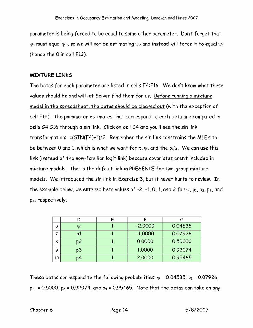
the example below, we entered beta values of -2, -1, 0, 1, and 2 for ψ, p1, p2, p3, and
p4, respectively.
6
7
8
9
10
D E F Gψ 1 -2.0000 0.04535p1 1 -1.0000 0.07926p2 1 0.0000 0.50000p3 1 1.0000 0.92074p4 1 2.0000 0.95465
These betas correspond to the following probabilities: ψ = 0.04535, p1 = 0.07926,
p2 = 0.5000, p3 = 0.92074, and p4 = 0.95465. Note that the betas can take on any

Exercises in Occupancy Estimation and Modeling; Donovan and Hines 2007
Chapter 6 Page 15 5/8/2007
value, and the link function constrains the MLE's to be between 0 and 1, which is
necessary because π, p1, p2, p3, p4,and ψ are probabilities, and probabilities range
between 0 and 1. The figure below shows betas that range from -9 to +9, and the
corresponding, sin “transformed” probability estimate. Look for the beta values of
-2, -1, 0, 1, and 2, and find their corresponding probabilities on the graph:
0
0.2
0.4
0.6
0.8
1
-10 -5 0 5 10
Beta
Pro
babi
lity
Now enter some numbers of your choice in the beta column (cells F4:F16) and
examine the MLE's. You should see that no matter what beta values you enter, the
corresponding parameters are constrained between 0 and 1.
Keep in mind that we don’t know what the beta values are…..we are going to let
Solver find the betas that maximize the multinomial log likelihood function (see
below). If the connection between betas and MLE’s is still rusty to you, go back to
Exercise 3 and review the material there…things will only get worse if you plow
ahead without understanding this very fundamental concept.
MULTINOMIAL LOGIT LINK

Exercises in Occupancy Estimation and Modeling; Donovan and Hines 2007
Chapter 6 Page 16 5/8/2007
OK, time for a little side comment. If you run heterogeneity models with more
than two groups, the sin or logit link won’t work. Why? Well, in our two-group
example, we estimate π as the proportion of study sites in mixture 1. If we know
the proportion of sites that belong to group 1, by definition we know the proportion
of sites that belong to group 2 (which is 1-π). Now, what if we had three groups?
We need to estimate the proportion of sites in group 1, group 2, and group 3. The
sum of these proportions must be 1. With two groups this was easily handled by
subtraction. But with three or more groups, there might be the potential, say, for
the proportion for group 1 to be 0.5 and the proportion for group 2 to be 0.7. This
won’t do. We need a special link that will force the sum of the proportions to equal
1. This link is called the multinomial link, and is what PRESENCE uses for any
heterogeneity model with three or more groups.
The multinomial logit link for a three group problem has the form:
Proportion in Group 1 = exp(B1)/(1 + exp(B1) + exp(B2))
Proportion in Group 2 = exp(B2)/(1 + exp(B1) + exp(B2))
Proportion in Group 3 = 1 – proportion in Group 1 – proportion in Group 2.
SPREADSHEET HISTORY PROBABILITIES
OK! Back to the spreadsheet. Now we are ready to compute the probability of
realizing each history. Let’s start with the first history listed, 1111, in cell B4.
The probability of realizing a 1111 history is estimated for each group separately.
If a site is in group 1, the probability of realizing a 1111 history is π ψ1 p1,1 p2,1 p3,1
p4,1. This equation is entered in cell H4: =G4*G6*G7*G8*G9*G10. If a site is in
group 2, the probability of realizing a 1111 history is (1-π) ψ2 p1,2 p2,2 p3,2 p4,2 This

Exercises in Occupancy Estimation and Modeling; Donovan and Hines 2007
Chapter 6 Page 17 5/8/2007
equation is entered in cell I4: =(1-G4)*G12*G13*G14*G15*G16. Some portion of
the 250 study sites will be in group 1, and some portion will be in group 2. Across
both groups, the probability of realizing a 1111 history is the sum of the two mixing
probabilities, given in cell J4 (=H4+I4). The natural log of the combined history
probabilities is computed in cells K4:K19.
Make sense? Spend time now clicking on the formula for each mixture, and be sure
to recognize that obtaining the final history probabilities depends on 1) the
proportion of sites in group 1 versus group 2, and 2) the estimates of ψ, p1, p2, and
p3 that are unique to each group.
Notice that the sum of cells J4:J19 must equal 1 (cell J20): there are 16 possible
histories, and each history has a probability of being realized, but the sum of the
probabilities must be 1.00.
THE MIXTURE MODEL MULTINOMIAL LOG LIKELIHOOD
The goal of the analysis, as you might have guessed, is to find the combination of
betas that maximizes the multinomial log likelihood function. Remember, by
changing the betas, we change the parameter estimates linked to each beta, which
changes the probability of each encounter history, which changes the LogeL.
Betas MLEs Encounter Histories LogeL
All that’s left is to compute the log likelihood, given the frequencies of each
history and the history’s probability. The multinomial log likelihood formula that
we’ve been using is in the blue box below.

Exercises in Occupancy Estimation and Modeling; Donovan and Hines 2007
Chapter 6 Page 18 5/8/2007
There are 16 terms in this function, one for each of the encounter histories. The
yi in the blue box are the frequencies of each kind of history and the pi in the blue
box equation above are the history probabilities. The LogeL is computed in cell B26
with the equation =SUMPRODUCT(C4:C19,K4:K19), which corresponds to the
general formula in the blue box. Now all we have to do is maximize this value to
find the MLE’s for our dataset.
MAXIMIZING THE LOG LIKELIHOOD
Before we run our first model, we need to make sure that ψ1 = ψ2, so set your
spreadsheet up as follows:
3
4
5
6
7
8
9
10
11
12
13
14
15
16
D E F GParameter Estimate? Betas MLE
π 1 =(SIN(F4)+1)/2
ψ 1 =(SIN(F6)+1)/2p1 1 =(SIN(F7)+1)/2p2 1 =(SIN(F8)+1)/2p3 1 =(SIN(F9)+1)/2p4 1 =(SIN(F10)+1)/2
ψ 0 =F6 =(SIN(F12)+1)/2p1 1 =(SIN(F13)+1)/2p2 1 =(SIN(F14)+1)/2p3 1 =(SIN(F15)+1)/2p4 1 =(SIN(F16)+1)/2
Mixture 2
Mixture 1
Make sure that the beta cells are cleared out. OK, now we’re ready to run this
model. We can call this model “ψ, p(t) – two groups” to indicate that we’re

Exercises in Occupancy Estimation and Modeling; Donovan and Hines 2007
Chapter 6 Page 19 5/8/2007
estimating π and ψ, plus p1, p2, p3, and p4 for each group. You know the drill. Open
Solver, and set cell B26 to a maximum by changing cells F4, F6:F10, F13:F16.
Press Solve and Solver will work through the various combinations of betas until it
finds the maximum.
MIXTURE MODEL OUTPUT
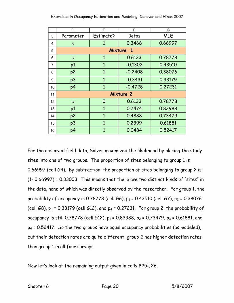
First, let’s take a look at the parameter estimates found by Solver:
Exercises in Occupancy Estimation and Modeling; Donovan and Hines 2007
Chapter 6 Page 20 5/8/2007
3
4
5
6
7
8
9
10
11
12
13
14
15
16
D E F GParameter Estimate? Betas MLE
π 1 0.3468 0.66997
ψ 1 0.6133 0.78778p1 1 -0.1302 0.43510p2 1 -0.2408 0.38076p3 1 -0.3431 0.33179p4 1 -0.4728 0.27231
ψ 0 0.6133 0.78778p1 1 0.7474 0.83988p2 1 0.4888 0.73479p3 1 0.2399 0.61881p4 1 0.0484 0.52417
Mixture 2
Mixture 1
For the observed field data, Solver maximized the likelihood by placing the study
sites into one of two groups. The proportion of sites belonging to group 1 is
0.66997 (cell G4). By subtraction, the proportion of sites belonging to group 2 is
(1- 0.66997) = 0.33003. This means that there are two distinct kinds of “sites” in
the data, none of which was directly observed by the researcher. For group 1, the
probability of occupancy is 0.78778 (cell G6), p1 = 0.43510 (cell G7), p2 = 0.38076
(cell G8), p3 = 0.33179 (cell G12), and p4 = 0.27231. For group 2, the probability of
occupancy is still 0.78778 (cell G12), p1 = 0.83988, p2 = 0.73479, p3 = 0.61881, and
p4 = 0.52417. So the two groups have equal occupancy probabilities (as modeled),
but their detection rates are quite different: group 2 has higher detection rates
than group 1 in all four surveys.
Now let’s look at the remaining output given in cells B25:L26.

Exercises in Occupancy Estimation and Modeling; Donovan and Hines 2007
Chapter 6 Page 21 5/8/2007
24
25
26
B C D E F G H I J K L
LogeL -2LogeL K AIC AICc -2LogeL Sat Deviance Model DF C-hat Chi-Square P value-611.24 1222.4847 10 1242.48 1243.41 1222.4472 0.0376 6 0.006259 0.0182 1.0000
OUTPUTS
The LogeL is given in cell B26. Cell C26 is -2 times cell B26, and is the -2LogeL. K
is the number of parameters in any given model, and the underlying equation is
=SUM(E4,E6:E10,E12:E16). AIC is computed as the -2LogeL + 2*K. AICc is the
second order correction of AIC, and uses the number of study sites in the
calculation. Deviance is computed as the difference between the saturated model’s
-2LogeL and the current model’s -2LogeL; the lower the number the better.
Remember that by definition the saturated model is a model in which the data “fit”
the model perfectly. The saturated model’s -2LogeL is computed in the usual way
(as in previous exercises) in cells N4:O21. The model we just ran had a deviance of
0.0376, which means it is about as good as you can possibly get. The Model
Degrees of Freedom is the number of unique histories minus K. In a model without
covariates, as long as the Model Degrees of Freedom is positive, you haven’t
overparameterized your model. C-hat is computed in cells J26 as Deviance divided
by DF. The C-hat in this case is close to 0. C-hats larger than 1 might indicate
some kind of lack of fit, which we don’t need to worry about for this example. The
Chi-Square statistic and associated p-value are given in cells K18:L18. The Chi-
square computations are provided in the orange cells L4:M19. As you can see, the
model results generate expected values that almost perfectly match the observed
values, so the chi-square value is about 0 (cell M20) and the p value is 1 (cell L26).
All in all, the parameters found by Solver provide a nearly perfect match to the
data (perhaps due to the fact that the data were generated with this exact model
by expectation!).

Exercises in Occupancy Estimation and Modeling; Donovan and Hines 2007
Chapter 6 Page 22 5/8/2007
Click on the button labeled Model 1 to add your results to the Results Table.
29
30
31
32
33
C D E F G H I JModel LogeL -2LogeL K AIC AICc Rank
1 ψ p(t)2groups -611.2489363 1222.497873 10 1242.498 1243.4184 12 ψ p(.)2groups #N/A3 ψ p(t) #N/A4 ψ p(.) #N/A
OK, now that you’ve run one model, we’ll run three more: a second mixture model
where p is estimated for each group, but is not time-dependent, and then the
standard models ψp(t) and ψp(.) models (with one group). Then we’ll run the same
analyses in PRESENCE to learn some very important concepts.
MODEL P(.)PSI FOR TWO GROUPS
In this model, we will estimate a single p for each group, and will force ψ to be
equal for both groups. That is, for group 1, p1,1 = p2,1 =p3,1, and for group 2, p1,2 =
p2,2 = p3,2. Think about how you would set this up in the spreadsheet.
3
4
5
6
7
8
9
10
11
12
13
14
15
16
D E F GParameter Estimate? Betas MLE
π 1 =(SIN(F4)+1)/2
ψ 1 =(SIN(F6)+1)/2p1 1 =(SIN(F7)+1)/2p2 0 =F7 =(SIN(F8)+1)/2p3 0 =F7 =(SIN(F9)+1)/2p4 0 =F7 =(SIN(F10)+1)/2
ψ 0 =F6 =(SIN(F12)+1)/2p1 1 =(SIN(F13)+1)/2p2 0 =F13 =(SIN(F14)+1)/2p3 0 =F13 =(SIN(F15)+1)/2p4 0 =F13 =(SIN(F16)+1)/2
Mixture 2
Mixture 1

Exercises in Occupancy Estimation and Modeling; Donovan and Hines 2007
Chapter 6 Page 23 5/8/2007
First, we must estimate π, so we enter a 1 in cell E4. Then, for mixture 1, we
estimate ψ, and enter a 1 in cell E6. Then we estimate p1, and enter a 1 in cell E7.
Then, we force p2, p3, and p4 in mixture 1 to be equal to p1 in mixture 1 and enter
0’s in cells E8:E10. For mixture 2, we force ψ for mixture 2 to be equal to ψ for
mixture 1. We will estimate p1, so we enter a 1 in cell E13. Then we force p2, p3,
and p4 to be equal to p1 for mixture 2. So, the total number of parameters to be
estimated for this model is 4. Let’s run it and see if it is more parsimonious than
the previous model. Open Solver, and set cell B26 to a maximum by changing cells
F4, F6:7, F13. Then Solve.
Now let’s look at the output:
Exercises in Occupancy Estimation and Modeling; Donovan and Hines 2007
Chapter 6 Page 24 5/8/2007
3
4
5
6
7
8
9
10
11
12
13
14
15
16
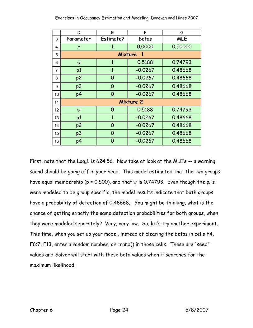
D E F GParameter Estimate? Betas MLE
π 1 0.0000 0.50000
ψ 1 0.5188 0.74793p1 1 -0.0267 0.48668p2 0 -0.0267 0.48668p3 0 -0.0267 0.48668p4 0 -0.0267 0.48668
ψ 0 0.5188 0.74793p1 1 -0.0267 0.48668p2 0 -0.0267 0.48668p3 0 -0.0267 0.48668p4 0 -0.0267 0.48668
Mixture 2
Mixture 1
First, note that the LogeL is 624.56. Now take at look at the MLE’s -- a warning
sound should be going off in your head. This model estimated that the two groups
have equal membership (p = 0.500), and that ψ is 0.74793. Even though the pij’s
were modeled to be group specific, the model results indicate that both groups
have a probability of detection of 0.48668. You might be thinking, what is the
chance of getting exactly the same detection probabilities for both groups, when
they were modeled separately? Very, very low. So, let’s try another experiment.
This time, when you set up your model, instead of clearing the betas in cells F4,
F6:7, F13, enter a random number, or =rand() in those cells. These are “seed”
values and Solver will start with these beta values when it searches for the
maximum likelihood.

Exercises in Occupancy Estimation and Modeling; Donovan and Hines 2007
Chapter 6 Page 25 5/8/2007
3
4
5
6
7
8
9
10
11
12
13
14
15
16
D E F GParameter Estimate? Betas MLE
π 1 =RAND() =(SIN(F4)+1)/2
ψ 1 =RAND() =(SIN(F6)+1)/2p1 1 =RAND() =(SIN(F7)+1)/2p2 0 =F7 =(SIN(F8)+1)/2p3 0 =F7 =(SIN(F9)+1)/2p4 0 =F7 =(SIN(F10)+1)/2
ψ 0 =F6 =(SIN(F12)+1)/2p1 1 =RAND() =(SIN(F13)+1)/2p2 0 =F13 =(SIN(F14)+1)/2p3 0 =F13 =(SIN(F15)+1)/2p4 0 =F13 =(SIN(F16)+1)/2
Mixture 2
Mixture 1
Now, run Solver again and see what happens. Here are our new results:
3
4
5
6
7
8
9
10
11
12
13
14
15
16
D E F GParameter Estimate? Betas MLE
π 1 0.2403 0.61899
ψ 1 0.6208 0.79085p1 1 -0.3156 0.34480p2 0 -0.3156 0.34480p3 0 -0.3156 0.34480p4 0 -0.3156 0.34480
ψ 0 0.6208 0.79085p1 1 0.3002 0.64786p2 0 0.3002 0.64786p3 0 0.3002 0.64786p4 0 0.3002 0.64786
Mixture 2
Mixture 1
You can quickly see that the MLE’s are different than the previous model run.
Each group now has unique detection parameters, as specified by the model. Also,

Exercises in Occupancy Estimation and Modeling; Donovan and Hines 2007
Chapter 6 Page 26 5/8/2007
it is important to note that the LogeL is 622.60, lower than the first model run. So
Solver found a solution in the first run that really wasn’t the maximum. The
results from PRESENCE match this second run. What happened is that Solver
found a local maximum in the first run – a point on a bumpy-shaped likelihood
surface that it thought was the peak, when unknown to it there was a slightly
higher peak somewhere else on the likelihood surface. On the second run Solver
found the true maximum.
Press the Model 2 button (around cell E19) to add your results to the Results
Table.
29
30
31
32
33
C D E F G H I JModel LogeL -2LogeL K AIC AICc Rank
1 ψ p(t)2groups -611.2489363 1222.497873 10 1242.498 1243.4184 12 ψ p(.)2groups -622.5977932 1245.195586 4 1253.196 1253.3589 23 ψ p(t) #N/A4 ψ p(.) #N/A
MODEL P(t)PSI (ONE GROUP)
OK, two more models to go, the first of which is the standard model ψ,p(t), just
like you ran in Exercise 3. In this model, all the sites belong to a single group, so
we will not be estimating π (we know it will be 1), and we will not be estimating any
of the parameters associated with group 2. So this model will estimate 5 total
parameters:

Exercises in Occupancy Estimation and Modeling; Donovan and Hines 2007
Chapter 6 Page 27 5/8/2007
3
4
5
6
7
8
9
10
11
12
13
14
15
16
D E F GParameter Estimate? Betas MLE
π 0 0.50000
ψ 1 0.50000p1 1 0.50000p2 1 0.50000p3 1 0.50000p4 1 0.50000
ψ 0 0.50000p1 0 0.50000p2 0 0.50000p3 0 0.50000p4 0 0.50000
Mixture 1
Mixture 2
OK, now to run this model, we will estimate all the betas uniquely, but will have to
add a constraint within Solver itself. Open Solver, and set cell B26 to a maximum
by changing cells F4, F6:F10, and F12:F16. This time, however, add the constraint
that cell G4 (π) must be equal to 1.
We added this constraint by clicking on the Add button within the Solver dialogue
box, typing in the constraints, and pressing the OK button:

Exercises in Occupancy Estimation and Modeling; Donovan and Hines 2007
Chapter 6 Page 28 5/8/2007
Now when you run Solver, you should get the following results:
3
4
5
6
7
8
9
10
11
12
13
14
15
16
D E F GParameter Estimate? Betas MLE
π 0 1.5708 1.00000
ψ 1 0.5094 0.74384p1 1 0.2060 0.60228p2 1 0.0540 0.52699p3 1 -0.0967 0.45171p4 1 -0.2497 0.37642
ψ 0 0.0000 0.50000p1 0 0.0000 0.50000p2 0 0.0000 0.50000p3 0 0.0000 0.50000p4 0 0.0000 0.50000
Mixture 1
Mixture 2
The only estimates that we need to be concerned with are the parameters
associated with group 1. As indicated, π is 1.000. It doesn’t matter what the
estimates are for mixture 2. Why? Because each history probability in mixture 2
is multiplied by 1-π, or 0. This is reflected in columns H and I, where only mixture
1 has non-zero history probabilities.
Go ahead and add the results of this model to the Results Table:

Exercises in Occupancy Estimation and Modeling; Donovan and Hines 2007
Chapter 6 Page 29 5/8/2007
29
30
31
32
33
C D E F G H I JModel LogeL -2LogeL K AIC AICc Rank
1 ψ p(t)2groups -611.2489363 1222.497873 10 1242.498 1243.4184 22 ψ p(.)2groups -622.5977932 1245.195586 4 1253.196 1253.3589 33 ψ p(t) -613.9628668 1227.925734 5 1237.926 1238.1716 14 ψ p(.) #N/A
You can see that this model beats the two mixture models (even though you’ll see
later that the data were simulated with strong mixture effects). We’ll explore
this more when we run the models in PRESENCE.
MODEL P(.)PSI (ONE GROUP)
OK, the last model is the one-group, constant p model, so you will be estimating
just two parameters. Go ahead and set this model up and run it. Don’t forget to
add the constraint that π = 1 within Solver. Here are our results:
3
4
5
6
7
8
9
10
11
12
13
14
15
16
D E F GParameter Estimate? Betas MLE
π 0 1.5708 1.00000
ψ 1 0.5188 0.74793p1 1 -0.0267 0.48668p2 0 -0.0267 0.48668p3 0 -0.0267 0.48668p4 0 -0.0267 0.48668
ψ 0 0.0000 0.50000p1 0 0.0000 0.50000p2 0 0.0000 0.50000p3 0 0.0000 0.50000p4 0 0.0000 0.50000
Mixture 1
Mixture 2
Click on the Model 4 button to add the results to the Results Table:

Exercises in Occupancy Estimation and Modeling; Donovan and Hines 2007
Chapter 6 Page 30 5/8/2007
29
30
31
32
33
C D E F G H I JModel LogeL -2LogeL K AIC AICc Rank
1 ψ p(t)2groups -611.2489363 1222.497873 10 1242.498 1243.4184 22 ψ p(.)2groups -622.5977932 1245.195586 4 1253.196 1253.3589 43 ψ p(t) -613.9628668 1227.925734 5 1237.926 1238.1716 14 ψ p(.) -624.5631978 1249.126396 2 1253.126 1253.175 3
Our top-ranked model is model ψ p(t), with an AICc score of 1238.2. The second
best model is the ψ p(t) two group mixture model, with an AICc score of 1243.4.
This is a difference of 5.2 AICc units; there is some support for the mixture
model, but it is not overwhelming. (This would be a good time to model average!).
Take a look at the LogeL’s of the two models.
29
30
31
32
33
C D E F G H I JModel LogeL -2LogeL K AIC AICc Rank
1 ψ p(t)2groups -611.2489363 1222.497873 10 1242.498 1243.4184 22 ψ p(.)2groups -622.5977932 1245.195586 4 1253.196 1253.3589 43 ψ p(t) -613.9628668 1227.925734 5 1237.926 1238.1716 14 ψ p(.) -624.5631978 1249.126396 2 1253.126 1253.175 3
The two group mixture model (model 1) had a LogeL of -611.2, whereas the top
ranked model (model 3) had a LogeL of -613.9. So model 1 “fit” the data better
than the top-ranked model (remember that it had a deviance of almost 0). But
because model 1 estimated 10 parameters compared to model 3 (which estimated 5
parameters), its AICc score was increased. We’ll explore the trade-offs between
model fit, number of parameters, and precision in PRESENCE.

Exercises in Occupancy Estimation and Modeling; Donovan and Hines 2007
Chapter 6 Page 31 5/8/2007
PRESENCE INPUT FILES
The histories and corresponding frequencies given in cells B4:B11
cannot be input directly into PRESENCE (most users of PRESENCE
include covariates in the analysis, so the input files are set up on a
site-by-site basis). So, we’ve entered some formulae in columns P:T
to convert the summarized data to site-specific data. But before we
cover the equations, first look at cells A2:A19, which are shaded
grey on the spreadsheet. These cells are a running tally of the total
number of sites in the study. Beginning with the first history (1111),
the cell A4’s formula counts the number of sites that are 1111. The
next cell (cell A5) counts the number of 1110 sites + the 1111 sites.
The next cell (cell A6) counts the number of 1101, 1110, and 1111
sites, and so on. We will use this running tally to create PRESENCE
input files.
Now let’s turn our attention to columns Q:V. In column Q, the sites
are listed from 1 to 250 down the column. In column R, we assign a history to each
site, using the tally in cells A3:A19. Click on cell R4. The equation there is
=LOOKUP(Q4-1,$A$3:$A$19,$B$4:$B$19). The function looks up the value in Q4
(the site number) minus 1 in the tally column (A3:A19), and then returns the
corresponding history listed in cells B4:B19. Because the lookup vector (the tally)
is sorted in ascending order, this equation “works” for our purposes because the
LOOKUP function doesn’t need to find an exact match. Take a look again at cells
B4:C19. Notice that there are 15 sites with a 1111 history, 17 sites with a 1110
history, 12 sites with a 1101 history, and so on. When the lookup function in column
R is copied down the column, the result is that the first 15 sites are given a 1111
2
3
4
5
6
7
8
9
10
11
12
13
14
15
16
17
18
19
ATally015324462708392112117126133148153165174250

Exercises in Occupancy Estimation and Modeling; Donovan and Hines 2007
Chapter 6 Page 32 5/8/2007
history, the next 17 sites are given a 1110 history, the next 12 sites are given a
1101 history, and so on. Given the histories in column R, columns S:V simply split
each history into survey-specific results (using LEFT, RIGHT, and MID functions).
When it’s time to create a PRESENCE input file, simply copy cells S4:V253 and
paste them into the PRESENCE datasheet.
3
4
5
6
7
8
Q R S T U VSite History Survey 1 Survey 2 Survey 3 Survey 4
1 1111 1 1 1 12 1111 1 1 1 13 1111 1 1 1 14 1111 1 1 1 15 1111 1 1 1 1
SIMULATING TWO GROUP MIXTURE DATA
OK, we’re almost finished with the spreadsheet exercise. The last section of the
spreadsheet is for simulating new data, either by expectation or with
stochasticity. Take a look at cells X3:AE6.
3
4
5
6
X Y Z AA AB AC AD AEParameter p1 p2 p3 p4 ψ N π
MLE Group 1 0.8 0.7 0.6 0.5 0.8 100 0.4MLE Group 2 0.4 0.35 0.3 0.25 0.8 150 0.6
Total Sites: 250
In this section of the spreadsheet, you enter parameter values (p1, p2, p3, ψ, N, and
π) for group 1 and for group 2. The data we’ve been analyzing in this exercise were
obtained from the parameter estimates shown above. Note that you make your
entries in the cells shaded in blue – the other cells are computed. For example, in
cell AD6, enter the total number of sites. In cell AE4, enter the proportion of
sites that are in group 1. Cell AE5 is computed as 1-π. Cells AD4 and AD5 are also
computed based on the entries for total sites and π.

Exercises in Occupancy Estimation and Modeling; Donovan and Hines 2007
Chapter 6 Page 33 5/8/2007
Given these entries, we can create data in two ways. First, we can create data
based on expectation.
8
9
10
11
12
13
14
15
16
17
18
19
20
21
22
23
24
25
26
AB AC AD AE AF
Mix 1 Mix 2 Total Rounded1111 13.44 1.26 14.7 151110 13.44 3.78 17.22 171101 8.96 2.94 11.9 121100 8.96 8.82 17.78 181011 5.76 2.34 8.1 81010 5.76 7.02 12.78 131001 3.84 5.46 9.3 91000 3.84 16.38 20.22 200111 3.36 1.89 5.25 50110 3.36 5.67 9.03 90101 2.24 4.41 6.65 70100 2.24 13.23 15.47 150011 1.44 3.51 4.95 50010 1.44 10.53 11.97 120001 0.96 8.19 9.15 90000 20.96 54.57 75.53 76
100 150 250 250
Summarized Expected Data:
Creating data based on expectation is really quite simple. In cells AB10:AB25, we
list the possible encounter histories. Then, given the parameter estimates
described above, we compute the number of sites in each group that should have a
particular history. For example, in cell AC10 we compute the number of sites in
mixture 1 that should have a 1111 history. The equation is
=AC4*Y4*Z4*AA4*AB4*AD4, which is N1 ψ1 p1,1 p2,1 p3,1 p4,1. In cell AD10 we
compute the number of sites in mixture 2 that should have a 1111 history. The

Exercises in Occupancy Estimation and Modeling; Donovan and Hines 2007
Chapter 6 Page 34 5/8/2007
equation is =AC5*Y5*Z5*AA5*AB5*AD5, which is N2 ψ2 p1,2 p2,2 p3,2 p4,2. In cell
AE10 we add the group 1 + group 2 sites. In cell AF10, we simply round the total
for data analysis purposes. The reason that the some of the models we ran earlier
fit so well is that we analyzed data created by expectation. As long as Solver finds
the MLE’s, the expected frequency of encounter histories should match the
observed frequency of encounter histories.
The second method of creating data for analysis is with some stochasticity. This
method is demonstrated in cells X29:AG279.
28
29
30
31
32
33
34
X Y Z AA AB AC AD AE AF AGHistory History Actual
Site Group rand() ψ rand() p1 rand() p2 rand() p3 rand() p4 1 2 History1 2 0.793062 0.606474 0.593843 0.7477917 0.80213 1100 0000 00002 2 0.750786 0.096962 0.845042 0.9888574 0.62718 1000 1000 10003 1 0.890587 0.887353 0.975259 0.814502 0.84084 0000 0000 00004 1 0.27869 0.090697 0.428131 0.153707 0.91658 1110 1010 11105 2 0.108711 0.748171 0.850801 0.9430909 0.28547 1001 0000 0000
In column X, we list the 250 sites. In column Y, we assign a group membership to
each site. Click on cell Y30 and you’ll see the formula =IF(RAND()<$AE$4,1,2). If
a random number is less than π (given in cell AE4), the site belongs to group 1,
otherwise it belongs to group 2. This formula is copied down for the remaining
sites until all 250 sites are assigned a group membership. As in previous exercises,
the next five columns (columns AA:AD are simply random numbers, with the
equation =RAND().
OK, now we’re ready to create an encounter history for each site. One easy way to
do that is to write out an encounter history for a site if it belongs to group 1
(column AE) and then to write a second encounter history for the same site if it
belongs to group 2 (column AF). The encounter histories follow the exact same

Exercises in Occupancy Estimation and Modeling; Donovan and Hines 2007
Chapter 6 Page 35 5/8/2007
logic as we discussed in the introduction of this exercise. Click on cell AE30. The
equation is: =
=IF(AND(Z30<$AC$4,AA30<$Y$4),1,0)&IF(AND(Z30<$AC$4,AB30<$Z$4),1,0)&I
F(AND(Z30<$AC$4,AC30<$AA$4),1,0)&IF(AND(Z30<$AC$4,AD30<$AB$4),1,0).
This formula should look at least vaguely familiar to you. It is composed of four
parts (written above in black, blue, red, and green -- one for each of the four
survey periods). Let’s look at the first part:
=IF(AND(Z30<$AC$4,AA30<$Y$4),1,0), which is a IF function with a nested AND
function within it. IF cell Z30 <$AC$4 (the random ψ for group 1 is less than the
specified ψ for group 1) AND if cell AA30 <$Y$4 (the random p1 is less than the
specified p1 for group 1), then return the number 1 (the species was detected);
otherwise return a 0 (the species was not detected). This portion of the formula
therefore returns a 1 or 0 for the first survey for site 1. The other portions of
the formula follow the same logic…work your way through them now. In column AF,
we repeat the exercise, but this time use the parameters associated with group 2.
Finally, in column AG, we assign the actual history for each site with a HLOOKUP
function. Click on cell AG30 and you’ll see the formula
=HLOOKUP(Y30,$AE$29:$AF$279,X30+1). This formula looks up the assigned
group membership for site 1 (listed in cell Y30) in a large table in which the first
column is either a 1 or a 2 (cells $AE$29:$AF$279). If the site is in group 1, the
function returns the history associated with group 1, and if the site is in group 2,
the function returns the history associated with group 2. If you haven’t used
HLOOKUP or LOOKUP functions yet, we encourage you to spend a bit of time
learning about them – they’re pretty handy functions for many tasks.

Exercises in Occupancy Estimation and Modeling; Donovan and Hines 2007
Chapter 6 Page 36 5/8/2007
The stochastic data are summarized in cells X10:Y26. If you create data this way,
copy cells Y10:Y25 and paste them into cells C4:C19 (the histories are ordered in
the same way). Then you can copy the data in columns Q:V for inputting into
PRESENCE.
8
9
10
11
12
13
14
15
16
17
18
19
20
21
22
23
24
25
26
X Y Z
1111 211110 141101 131100 201011 71010 131001 141000 250111 30110 60101 50100 180011 30010 150001 100000 63
250
Summarized Stochastic Data:

Exercises in Occupancy Estimation and Modeling; Donovan and Hines 2007
Chapter 6 Page 37 5/8/2007
SINGLE SEASON OCCUPANCY MODELS ANALYSIS IN PRESENCE
OBJECTIVES
• To become familiar with PROGRAM PRESENCE
• To run the two group, single-season occupancy model in PRESENCE
• To understand the PRESENCE mixture model output.
• To review concepts of model selection.
GETTING STARTED
In this exercise, we will be analyzing the data we explored in the previous
(spreadsheet) chapter. When you open PRESENCE, you’ll see the following screen:
Choose File | New Project, and you’ll see the following screen:

Exercises in Occupancy Estimation and Modeling; Donovan and Hines 2007
Chapter 6 Page 38 5/8/2007
Enter a title for the analysis (e.g., “Two group mixture models”). Then enter 250
for No. Sites and 4 for No. Occasions. Then click on the button labeled “Input
Data Form”:
Now you are ready to paste in your spreadsheet data. Return to the spreadsheet
and copy cells S4:V253. Then return to the data entry page in PRESENCE, and
Exercises in Occupancy Estimation and Modeling; Donovan and Hines 2007
Chapter 6 Page 39 5/8/2007
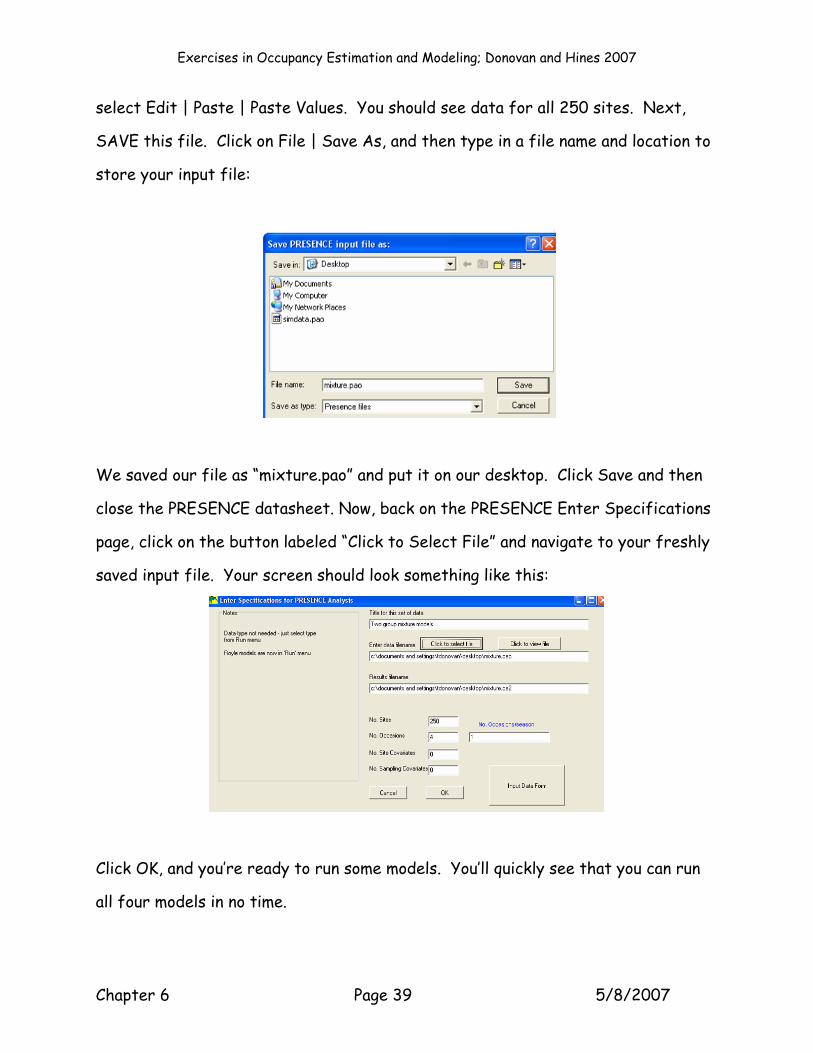
select Edit | Paste | Paste Values. You should see data for all 250 sites. Next,
SAVE this file. Click on File | Save As, and then type in a file name and location to
store your input file:
We saved our file as “mixture.pao” and put it on our desktop. Click Save and then
close the PRESENCE datasheet. Now, back on the PRESENCE Enter Specifications
page, click on the button labeled “Click to Select File” and navigate to your freshly
saved input file. Your screen should look something like this:
Click OK, and you’re ready to run some models. You’ll quickly see that you can run
all four models in no time.

Exercises in Occupancy Estimation and Modeling; Donovan and Hines 2007
Chapter 6 Page 40 5/8/2007
MODEL P(t)PSI FOR TWO GROUPS
Our first model is the two-group mixture model where t is uniquely estimated for
each group. To run this model in PRESENCE, choose Run | Analysis from the main
toolbar, and then select the pre-defined model named 2 groups, Survey-specific P.
Make sure the “Set digits in estimates” in NOT checked. Click “OK to Run”.
Wasn’t that easy? Add your results to the Results Browser:
Now, right-click on the model name to pull up the model results:

Exercises in Occupancy Estimation and Modeling; Donovan and Hines 2007
Chapter 6 Page 41 5/8/2007
PRESENCE indicates that this is a two-group, predefined model with 250 study
sites, 4 sampling occasions, 0 missing observations, and 10 parameters. Note the
starred sentence that reads, “Numerical convergence may not have been reached.
Parameter estimates converged to approximately 2.735163
significant digits.” This is an important warning. It means that the optimization
program may not have found the peak of the likelihood surface because the log
likelihood value was still changing after the specified number of iterations. You
have to decide whether 2 significant digits are enough to satisfy you. (We’re fine
with two significant digits, but get in the habit of reading this warning and not
blindly skipping over it).
Note: If you want to improve the precision of the estimates even more, delete the
model you just ran from the Results Browser (right-click on the model name and
select “delete”), and re-run the model. But this time, click on the option labeled

Exercises in Occupancy Estimation and Modeling; Donovan and Hines 2007
Chapter 6 Page 42 5/8/2007
“Set function evaluations” on the run page and increase the number of functions
that will be evaluated.
OK, now let’s compare these results to the spreadsheet:
Although we haven’t shown it, the -2LogeL, AIC and naïve estimates match, and you
can see above that the MLE’s match as well. Note that PRESENCE estimated π
(which is labeled theta) as 0.3300 for group 1, and 1-π = 0.6700 for group 2. The
spreadsheet estimated π as 0.6700. It doesn’t matter which group is which, as
long as you match the correct, corresponding MLE’s with each group.
You might also recall from the spreadsheet exercise that this model had a very,
very low Deviance score – the model fits the observed field data almost perfectly.
But at what price? Take a look now at the standard errors associated with each
parameter……they are VERY large for all of the detection parameters. For
instance, p1,1 (in PRESENCE) is estimated as 0.8399, with a standard error of
0.277. This corresponds to a lower 95% confidence interval of 0.8399 - 1.96 *
3
4
5
6
7
8
9
10
11
12
13
14
15
16
D GParameter MLE
π 0.66997
ψ 0.78778p1 0.43510p2 0.38076p3 0.33179p4 0.27231
ψ 0.78778p1 0.83988p2 0.73479p3 0.61881p4 0.52417
Mixture 1
Mixture 2

Exercises in Occupancy Estimation and Modeling; Donovan and Hines 2007
Chapter 6 Page 43 5/8/2007
0.277= 0.2969 and an upper 95% confidence interval of 0.8399 + 1.96 * 0.277=
1.383. We wouldn’t put much confidence in the 0.8399 estimate.
The take-home message is these models really need a lot of sites in order to work
reasonably well. Even with the large differences in the p's in this example, the
standard errors are pretty big. Would this model be selected as the best model in
a model selection exercise? Probably not (as you’ve seen from the spreadsheet
runs), because 10 parameters were estimated to make the model more “realistic”.
Furthermore, each of the 10 parameters has poor precision (high standard errors).
In other words, adding complications to the model to make it more realistic comes
at a price - not being able to estimate those parameters as well (i.e. high
variances). Let’s run the remaining models and then study the Results Browser in
detail.
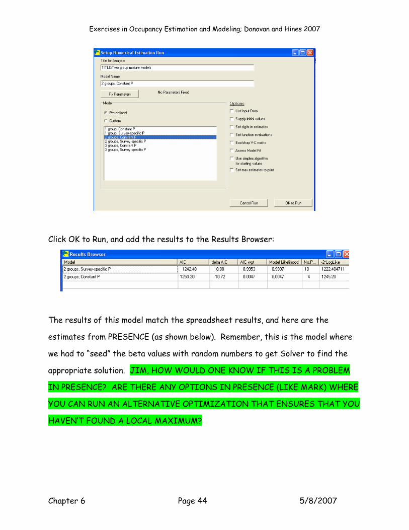
MODEL P(.)PSI FOR TWO GROUPS
OK, our next model is the two-group constant p model, which is another pre-
defined model in PRESENCE. (In fact, the mixture models are all pre-defined – you
can try to customize the mixture model in the Design Matrix and will quickly see
that you can’t run anything but the pre-defined models). Go to Run | Analysis –
Single-Season and select the 2-group, Constant-P model.
Exercises in Occupancy Estimation and Modeling; Donovan and Hines 2007
Chapter 6 Page 44 5/8/2007
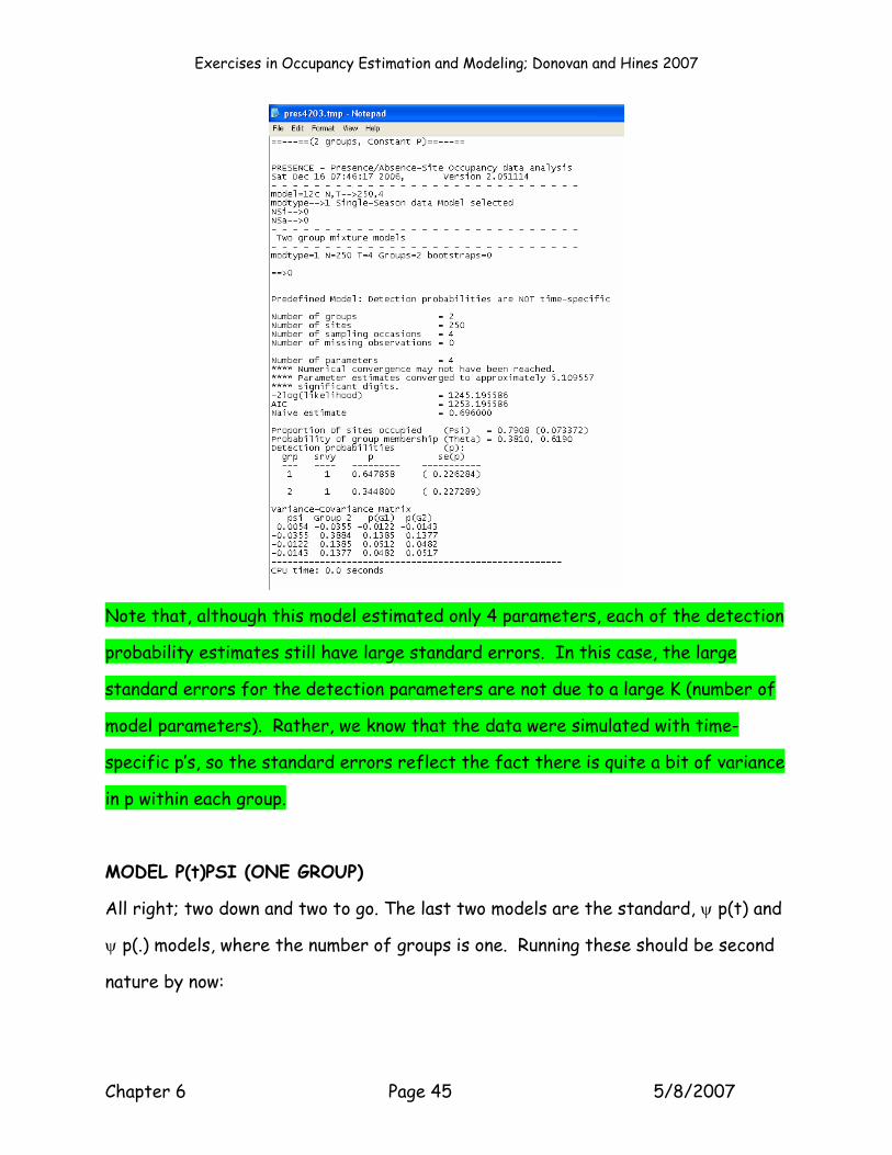
Click OK to Run, and add the results to the Results Browser:
The results of this model match the spreadsheet results, and here are the
estimates from PRESENCE (as shown below). Remember, this is the model where
we had to “seed” the beta values with random numbers to get Solver to find the
appropriate solution. JIM, HOW WOULD ONE KNOW IF THIS IS A PROBLEM
IN PRESENCE? ARE THERE ANY OPTIONS IN PRESENCE (LIKE MARK) WHERE
YOU CAN RUN AN ALTERNATIVE OPTIMIZATION THAT ENSURES THAT YOU
HAVEN’T FOUND A LOCAL MAXIMUM?
Exercises in Occupancy Estimation and Modeling; Donovan and Hines 2007
Chapter 6 Page 45 5/8/2007
Note that, although this model estimated only 4 parameters, each of the detection
probability estimates still have large standard errors. In this case, the large
standard errors for the detection parameters are not due to a large K (number of
model parameters). Rather, we know that the data were simulated with time-
specific p’s, so the standard errors reflect the fact there is quite a bit of variance
in p within each group.
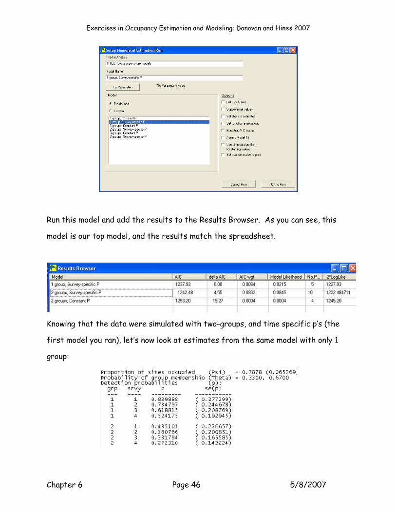
MODEL P(t)PSI (ONE GROUP)
All right; two down and two to go. The last two models are the standard, ψ p(t) and
ψ p(.) models, where the number of groups is one. Running these should be second
nature by now:
Exercises in Occupancy Estimation and Modeling; Donovan and Hines 2007
Chapter 6 Page 46 5/8/2007
Run this model and add the results to the Results Browser. As you can see, this
model is our top model, and the results match the spreadsheet.
Knowing that the data were simulated with two-groups, and time specific p’s (the
first model you ran), let’s now look at estimates from the same model with only 1
group:
Exercises in Occupancy Estimation and Modeling; Donovan and Hines 2007
Chapter 6 Page 47 5/8/2007
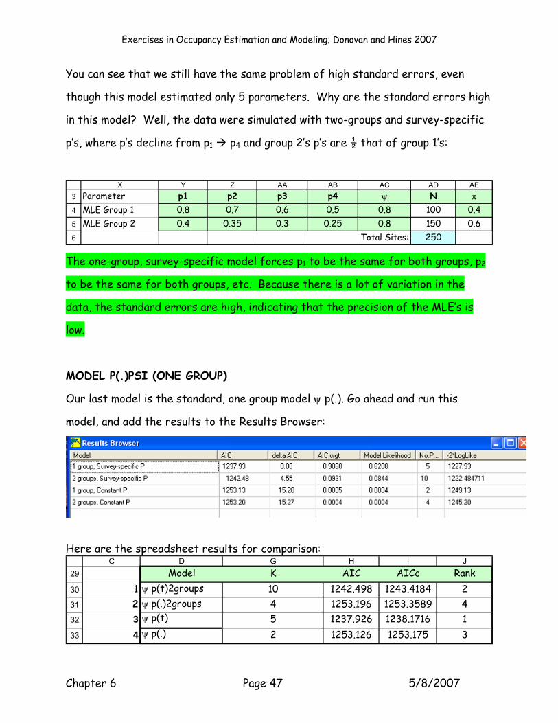
You can see that we still have the same problem of high standard errors, even
though this model estimated only 5 parameters. Why are the standard errors high
in this model? Well, the data were simulated with two-groups and survey-specific
p’s, where p’s decline from p1 p4 and group 2’s p’s are ½ that of group 1’s:
3
4
5
6
X Y Z AA AB AC AD AEParameter p1 p2 p3 p4 ψ N π
MLE Group 1 0.8 0.7 0.6 0.5 0.8 100 0.4MLE Group 2 0.4 0.35 0.3 0.25 0.8 150 0.6
Total Sites: 250
The one-group, survey-specific model forces p1 to be the same for both groups, p2
to be the same for both groups, etc. Because there is a lot of variation in the
data, the standard errors are high, indicating that the precision of the MLE’s is
low.
MODEL P(.)PSI (ONE GROUP)
Our last model is the standard, one group model ψ p(.). Go ahead and run this
model, and add the results to the Results Browser:
Here are the spreadsheet results for comparison:
29
30
31
32
33
C D G H I JModel K AIC AICc Rank
1 ψ p(t)2groups 10 1242.498 1243.4184 22 ψ p(.)2groups 4 1253.196 1253.3589 43 ψ p(t) 5 1237.926 1238.1716 14 ψ p(.) 2 1253.126 1253.175 3

Exercises in Occupancy Estimation and Modeling; Donovan and Hines 2007
Chapter 6 Page 48 5/8/2007
The bottom line is that these mixture models really need a lot of data to perform
well in a model-selection exercise. The number of parameters that are estimated
can get very large, very quickly, resulting perhaps in a better-fitting model (lower -
2LogeL’s) but at a cost: the standard errors can be quite large, with low precision.
That wraps up this exercise. Hopefully you have a good idea of what mixture
models are all about and can use them wisely in your own work.