'I

, 1•. \ )

PORECASTZNG CROP ACREAGES AND YZELDS ZN THE FACE OF AND ZN SPZTE OFFLOODS

Rich Allen, Deputy Administrator for ProgramsNational Agricultural statistics Service (NASS) 1/

ZNTRODUCTZON

The 1993 growing season presented some of the most difficultchallenges ever for forecasting United states crop production.This paper will describe on-going crop forecasting and estimationprograms and procedures of the National Agricultural statisticsservice (NASS) of the United states Department of Agriculture alongwith modifications that were made in 1993 because of weatherconcerns. Performance of the 1993 procedures will be analyzed~both as far as consistency throughout the season and compared toend-of-season estimates.To briefly summarize, NASS procedur.es did work extremely well forestimating crop acreage not planted and planted acreage lost toflooding and for forecasting the acreage expected to be harvestedand the numbers of corn ears and soybean pods to be harvested.-Timing 'of the floods in the midwest was such that usual surveytiming could be used. The Secretary of Agriculture agreed to waitfor NASS regular report dates rather t~an early evaluations whichcould not be as statistically based. Increases in sample sizeswere made to improve precision of acreage data published in Augustand additional questions on acreage' plans were added each monththroughout the growing season. What did not perform as well asdesired were forecasts of weight of fruit at harvest, particularlycorn weight of grain per ear. The paper will present some reasonsthat the weight forecasts were not better.CROP ESTDIATZON HZSTORY

The USDA has been issuing agricultural statistics since its.founding in 1862. One original reason for creation of theDepartment was compilation and dissemination of statistics. The

1/ Any opinions or judgements expressed in this paper are those ofthe author and do not necessarily reflect those of the NationalAgricultural Statistics Service or the United States Depar~entof Agricul ture. Reference to any commercial products is forcompleteness only and does not consti tute an endorsement ofthese products.

Special thanks are extended to TomBirkett, Mike Craig, BillDowdy, Gary Keough, and Charles Van Lahr for their suggestionsand assistance with examples and to Mary Ann Higgs for typingand editorial assistance.

first crop report was issued in July 1863. Monthly reports up toabout 1911 reported crop condition compared to normal. End-of-season production estimates were based on comparisons to theCensuses of Aqriculture conducted at 10 year intervals.In the early 1900's, USDA was able to produce end-of-seasonestimates based on larqe samples of reports and improve on earlierprocedures since both acreaqe harvested and yield per acre wereestimated. startinq in 1911, monthly crop condition data wereconverted to yield per acre forecasts by comparison with 10-yearcondition averaqes. By 1925 the monthly Farm Report survey wasimplemented which was a fixed panel of farmers representinq allproducinq areas. The Farm Report provided monthly livestock andlabor information as well as yield forecasts. La~qer samples wereselected at plantinq and harvest to better measure actual acreaqesand production. -In the early 1960's, "objective yield" surveys were introduced forcrops such as corn, soybeans, wheat, and cotton in States with theqreatest acreaqes. These surveys establish small sample units inrandomly selected fields which are visited monthly to determinenumbers of plants, numbers of fruit (wheat heads, corn ears,soybean pods, etc.), and weiqht per fruit. Forecastinq models are-based on relationships of samples of the same maturity staqe incomparable months durinq the past 5 years in each State. Thosesurveys are currently conducted in States which account for about70-80 percent of the crop acreaqe.Also in the early 1960's, the Aqency implemented a mid-year AreaFrame survey. This enabled creation of probability based acreaqeestimates for the first time. Samplinq errors for major crops areas low as 1 percent at the U.S. level with levels of 2 to 3 percentin the larqest producinq States. Table 1"presents the 1993 cornand soybean planted acreaqe coefficients of variation for selected .States and the u.S.Matchinq area frame operations aqainst list frame samples since the

.early 1970's allows the creation of multiple frame estimates.Table 2 presents the 1993 corn and soybean acreaqe coefficients ofvariation from the midyear multiple frame survey for selectedStates and the u.S.The Farm Report panel survey was used up to the late 1980's in allStates. However, testinq of a probability selected, inteqratedsamplinq and survey approach which combined hoq and piq, qrainstocks, and crop acreaqe and production surveys, includinq monthlyyield forecasts, beqan in 1985 and was implemented for all Statesby 1990. After a period of overlap in each State, the Farm Reportsample was discontinued.

- 2 - -

•.1

Table 1.--Precision of 1993 J~ne Enumerative Survey Planted Acreage Expansions

Sununary Level Number of Coefficients of VariationSegments

Corn I SoybeansPercent

Illinois 389 2.5 2.8Indiana 294 3.5 3.6Iowa 437 1.9 2.6Kansas 456 11.1 7.9Minnesota 343 4.0 4.7Missouri 387 6.3 4.2Nebraska 390 3.9 - 5.3-North Dakota 376 13.6 17.9Ohio 289 4.5 4.1South Dakota 352 6.1 7.5Wisconsin 310 4.7 12.610 OY Corn States 3.503 1.28 OY Soybean States 2.924 1.3u.S. 1'5.462 1.1 1.2

Table 2.--Precision of 1993 June Multiple Frame Planted Acreage Expansions

Coefficients of VariationSummary Level Corn I Soybeans

PercentIllinois 1.9 .2.0Indiana 2.3 2.7Iowa 2.0 2.3Kansas 6.4 6.2Minnesota 2.7 3.2Missouri 4.7 4.2Nebraska 2.5 3.3North Dakota 6.7 9.0Ohio 3.2 .3.7South Dakota 3.0 4.0Wisconsin 2.8 6.310 OY Corn States 0.88 OY Soybean States 1.1U.S. 0.7 0.9

- 3 -

1 'r

It

•II••

CROP BSTIMATING/PORBCASTING CYCLBNASS is known for ontime delivery of its statistical reports. ByNovember of each year, release dates and times are published forthe nearly 400 reports which will be issued by its Agriculturalstatistics Board the next year. It is a rare occurrence if NASShas to delay the rel~ase of any scheduled reports.For spring,planted crops, the annual estimating/forecasting cyclestarts with Prospective Plantinas. Data are collected the firsttwo weeks of March on farmers' current intended plantings. Thisreport, issued at the end of March, is the first solid informationon how farmers plan to adjust to current market conditions,government farm programs changes, and other information.An interesting and much used report which relates to the springplanted crops is the Weeklv Weather and Crop Bulletin. Arelatively small panel survey is conducted each week·from plantingthrough harvest. Reporters fill out questionnaires on Fridayswhich are summarized on Monday mornings in order to provide anupdate on crop progress and crop conditions. A tabular summary ofcrop progress and conditions in the most significant states ofmajor crops is released late on Monday afternoon. This weekly,report does not create acreage estimates or yield forecasts.The June Agricultural Survey provides information on actualacreages of spring planted crops. Most planting of major crops hasoccurred by early June but there is always some planting left,particularly for soybeans planted after harvest of winter wheat insome states. Farmers are asked to report actual plantings to thetime of the interview and their intentions for the rest of theiracreage. The Acreaae report, with u.s. and State data, is issuedat the end of June. There often is not much flexibility to shiftplanting plans since preparation for corn planting may involvechemicals that would prohibit the planting of soybeans. If.planting is delayed too much due to bad weather (includingconditions being too dry to plant soybeans after wheat harvest)

.some intended acreage might not be planted.It might be helpful to point out the relationship of other USDAreports to NASS reports. Corn and soybean crops (and many otherspring planted crops) are not advanced enough to statisticallymeasure and forecast yields until about August 1. However, thereis a need in USDA to have an earlier working figure on potentialcrop size. That figure is provided by the World AgriculturalOutlook Board (WAOB) starting in its May World Aaricultural SUD~lyand Demand Estimates report issued concurrently with ~e NASS CrODProduction report. The WAOB uses an expert panel approach toassimilate all information available for major crop producing,importing, and exporting countries. Data sources includeagricultural attache reports, official foreign country statistics,

- 4 -

L {

,"' II,.."

','

"

weather data, computer models, and some remote sensinqinterpretations. In May, the WAOB uses the ProsDective Plantinasplanted acreaqe figures as a base and interprets acreaqe to beharvested and trend yields. In July, WAOB updates its projectionsby usinq the Acreage report for acreaqe and modifyinq trend yieldmodels for observed weather. Only u.s. yieldS are projected by theWAOB. Startinq in A~qust, NASS forecasts state yields as well asu.s. averaqes.NASS forecasts the yields of most sprinq planted crops monthly fromAuqust to November. (Cotton forecasts continue throuqh January.)Data collection starts about the 22nd of the precedinq month forobjective yield samples and about the 25th for farmer interviews.Data collection must be finished by about the third of the month inorder to edit, process, and interpret all data~in time for themonthly CrOD Production report which by law must be issued be~weeJ1the 8th and 12th of the month •..NABS policy is that monthly forecasts are based on data collectedabout the first of the month and assuminq "normal" weather afterdata collection. Sayinq that another way, NASS staff members donot chanqe indicated forecasts based on assumptions about weatherfor the rest of the season.NASS does not revise monthly yield forecasts since no new data willever be collected for that forecast. Instead, the forecast basedon conditions as of the first of this month will be replaced bynext month's forecast based on conditions at the end of this month.NASS covers all producinq States the first month of the forecastseason. However, some "limited forecast" States are desiqnated formost crops. Limited forecast States individually have less thanone-half of 1 percent of the u.s. acreaqe and collectively haveabout 3 percent or less of the total acreaqe. The data collection,analysis, and interpretation costs are saved in those States afterthe first month since the first forecast is carried forward untilthe end of the season.

"The end-of-season survey for most sprinq planted crops is theAqricultural Survey in December. Aqain, information is collecteddurinq the first half of December but in this case, the Cro'9Production - Annual is not issued until the January Crop Productionrelease about the 10th of January. One reason for this delayedrelease timinq is the holiday season at the end of D~cember andearly January. However, the more important aqricultural reason isthat several important crop related reports are all released at thesame time: CrOD Production - Annual, Grain stocks, January bropProduction report which has the updated cotton for~cast,RiceStocks, and winter Wheat and Rye Seedings plus the January WorldAgricultural SUDDlv and Demand Estimates. Issuing all reports atone time allows NASS staff members to perform improvedinterpretation across reports and gives data users a full pictureof information at one time.

- 5 -

'1 .,

""/'

The discussion above describes each year from a lO9ical cropphenology standpoint. However, the NASS survey cycle actuallystarts in June. That is the one time each year when NASS visitsall 15, 000 plus area frame segments. These segments are typicallyabout one square mile in size in intensively cultivated areas.Each state has been stratified by land use and segment sizes andsampling rates vary c.onsiderably by strata. This June EnumerativeSurvey is one of the most effective ongoing government surveys.Boundaries of sampling units are shown on aerial phot09raphs sonearly all nonsampling errors can be avoided. All fields withinsampling units are sketched on the aerial photos which againcontrols nonsampling errors. This survey collects precise field-by-field information on crops planted or other utilization. Mostobjective yield samples are selected from the area frame. Table 3shows the area frame stratification, average sampling unit sizes,and number of sampling units in the survey for Ohio. The s'Crat~definitions and samplinq rates for Ohio are fairly typical.Nationally, between one-third and one-half of 1 percent of theagricultural sampling units are selected.

Table 3.--1993 Area Frame Sample for Ohio

Stratum Definition Average Segment Segments in Segments inSize Population Sample

Sq. Miles -

>75% Cultivated51-75% Cultivated15-50% CultivatedAgri-Urban:>20 Home/SqmiResort:>20Home/Sqmi<15% CultivatedNon-AgriculturalTotal Sample

1.001.001.000.100.251.000.50

1433862766625

12229345

6205143

1055530102

102

289

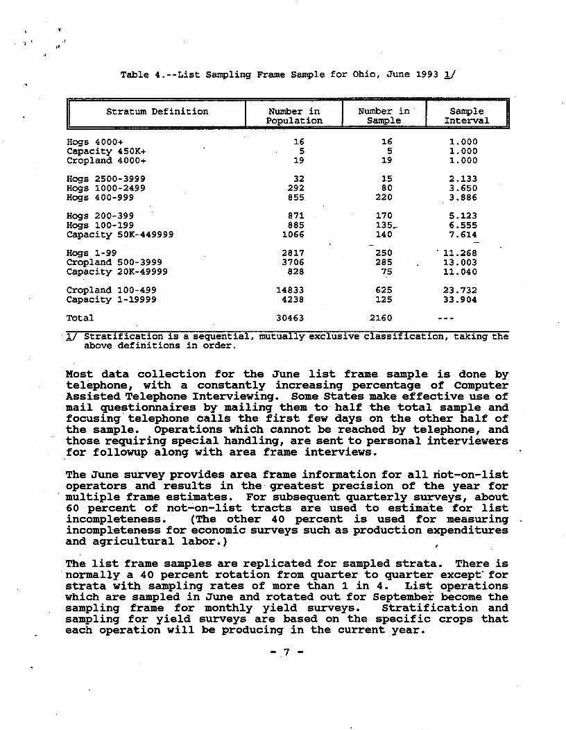
Typically, about 130,000 total tracts (areas of land within asegment under one operator) are found in this June EnumerativeSurvey with over 50,000 being agricultural tracts. The list framesample in June is about 75,000 operators. stratification is doneon a State-by-State basis to allow each State to properly reflectthe relative importance of medium and large hog operations· andcover specific crops that are of particular importance in theState. Table 4 shows the list frame strata and sampling rates forOhio in June 1993. Table 4 indicates that hogs are given much ofthe higher priorities in this integrated design; most of the largerhog farms would also have sizable crop acreages.

- 6 -

1 •

'.<

Table 4.--List Sampling Frame Sample for Ohio, June 1993 1/

Stratum Definition Number in Number in SamplePopulation Sample Interval

HogS 4000+ 16 16 1.000Capacity 450K+ 5 5 1.000Cropland 4000+ 19 19 1.000Hogs 2500-3999 32 15 2.133Hogs 1000-2499 292 80 3.650Hogs 400-999 855. 220 3.886Hogs 200-399 871 170 5.123Hogs 100-199 885 135,- 6.555Capacity 50K-449999 1066 140 7.614Hogs 1-99 2817 250 - 11.268Cropland 500-3999 3706 285 13.003Capacity 20K-49999 828 75 11.040Cropland 100-499 14833 625 23.732Capacity 1-19999 4238 125 33.904Total 30463 2160

-1/ Stratification is a sequential, mutually exclusive classification, taking theabove definitions in order.

Most data collection for the June list frame sample is done bytelephone, with a constantly increasing percentage of ComputerAssisted Telephone Interviewing. Somestates makeeffective use ofmail questionnaires by mailing them to'half the total sample andfocusing-telephone calls the first few days on the other half ofthe sample. Operations which cannot be reached by telephone, andthose requiring special handling, are sent to personal interviewersfor followup along with area frame interviews.

TheJune survey provides area frame information for all riot-on-listoperators and results in the greatest precision of the year formultiple frame estimates. For subsequent quarterly surveys, about60 percent of not-on-list tracts are used to estimate for listincompleteness. (The other 40 percent is used for measuringincomp~eteness for economicsurveys such as production expendituresand agricultural labor.)

The list frame samples are replicated for sampled strata. There isnormally a 40 percent rotation from quarter to quarter except' forstrata with sampling rates of more than 1 in 4. List operationswhich are sampled in June and rotated out for september becomethesampling frame for monthly yield surveys. Stratification andsampling for yield surveys are based on the specific crops thateach operation will be producing in the current year.

- 7 -

• •

'.'

\'

since June acreage information is available for all operations inthe monthly yield survey, reinterviews for the August 1 CropProduction report provide a natural planted acreage uPdate. TheAugust 1 survey also estimates the amount of acreage intended forharvest for corn for grain and for soybeans. Since there isusually little abandonment of acreage during the season, theacreage questions ar~ normally not repeated after August. Farmersare asked each month to report their expected average yield ortheir total production.For corn and soybean objective yield States, a self-weightingsample of fields is drawn from the expanded June area frame data.This ensures a good geographic dispersion within each State andsimplifies summary calculations.The September Agricultural Survey does not collect any corn andsoybeans production information but focuses on 'small grain end-of-season production data plus grain stocks and hogs and pigs. TheDecember Agricultural Survey collects actual acreages harvested andproduction data for corn, soybeans, and other spring planted crops.The u. S. sample size in December is normally about 82,000 with75,000 coming from the list sampling frame and 7,000 area not-on-list operations. Part of the December list sample will have been

,surveyed in June and part in September so identicals can becalculated but the major indication is the direct expansion.The March Agricultural Survey completes the survey cycle. It hasa total sample size of about 77,000, collecting intended plantingsinformation in addition to grain stocks and hogs and pigs.1993 EARLY SBASO. WBATBER

For most of this paper, comparisons will be made to averages fromrecent years with specific comparisons made to the 1992 season.This is because the 1992 season itself was one of the most unusualin memory. It was a cool year with crop progress being quite slow.However, killing frosts did not occur until later than' normal and

,record level yieldS were produced. The 1992 season had to be aninfluence in farmer yield forecast evaluations during 1993 and the1992 results were built into objective yield forecasting modelsalong with the previous four years.The 1993 growing season was cool and moist throughout most of themidwest States. Planting did not get off to an early start and itprogressed much slower than normal, particularly in the States ofIowa, Minnesota, and South Dakota. Planting average for the U.S.was about 2 weeks behind normal in early May and still a weekbehind at the end of May. Figures 1 to 4 present the plantingprogress in the States of Illinois, Iowa, Minnesota, and for the 17corn producing States with comparable data.

- 8 -

(

1993 CORN PLANTING PROGRESS 1/

Figure 1 United States Figure 2 Illinois

o414411' 411''''' SI2 SJI S/1. SJ2S1/30 fit 1/1S

too

so :: .

10 ................•..............

40 ........•..•...•.•......•.

·'112+ '113·SYRAVQ

tOO

10 .

10 .

40 .....••..•..•.•..••

• tlt2+'113·SYRAVQ

4111411' ..,. SJ2 SJI 1/11 IllS S/3O fit 1111

·'1.+1113·SYRAVG

411' ..,. SI2 SJI S/11 1m S/3O 1/1 1/1S

·,1.I +'1"

·SYRAVQ4111411. 4125 SJ2 SII SNI sm S/3O 1/' I/ts

MinnesotaFigure 4

,..Iowa

40 ........•....•..

Figure 3

10 .

100

11 Based on Weekly Weather Crop Survey.

9 -

I' ,"

At the time of the 1993 June Enumerative Survey interviews, 95percent of'the U.S. corn crop and 65 percent of the U.s. soybeanswere planted. These figures match up well with indications fromthe Weekly Weather Crop during the same period.The cool, damp early season weather turned to heavy rains andflooding in at least.nine States (South Dakota, Nebraska, Kansas,Minnesota, Iowa, Missouri, Wisconsin, Illinois, and North Dakota).The North Dakota flooding was more isolated than in the otherStates. North Dakota will not be included in some of thecomparisons in this paper since it has limited corn and soybeanacreages and is not in the objective yield program for eitl1ercrop.These nine states produced 77 percent of the 1992 U.S. corn cropand 64 percent of the 1992 U.S. soybean crop.At the time of the Acreaae report on June -30, there were- fewquestions about the numbers publiShed •. However, there wereconcerns that some acreage intended to be planted had'not and wouldnot be planted. Ever since 1980, the June acreage estimates ofcorn plante~ acres had been within plus or minus 1 percent of thefinal planted acreage estimate. Even soybeans, which can beaffected by double cropping decisions made after mid-June, hadexceeded a 1 percent change only twice since 1980.AUGUST 1 ACREAGB BSTXMATBSsince 1990, the normal NASS survey program collects additionalinformation on plantings by including those questions on themonthly yield survey in August. All operators in that sample didreport in the list portion of the June Agricultural Survey sodirect comparisons can be made.Because of weather concerns in late June and July, NASS expandedits data collection for the August 1 survey. For the nine floodStates, all area.frame tracts (operations) which had not completed .planting in June were recontacted. This area frame update was partof usual procedures until 1987 when the start of the June

.Enumerative Survey was moved from about May 20 to June 1. Therehas not been a great need for an acreage update since.In order to strengthen information from the list frame, an extrareplicate was selected to be contacted August 1 along with thenormal monthly ag yield survey sample. All corn and soybeanobjective yield sample interviews (which include acreage updateinformation) were conducted about August 1 instead of the u~ualpattern of starting half of the samples August 1 and the remainderseptember 1. An additional objective yield like sample which wasscheduled for interviews in September or'October for agriculturalchemical use data was also contacted for August 1 acreage data.Table 5 presents the total contacts designated for August 1.

- 10 -

-'

Table 5.--August 1 Survey Contacts Made to Update Planted Acreage Information 11

Growers Corn SoybeanState Area Frame Subsampled Objective Objective

Operations from June Yield YieldList Survey Survey Survey

Illinois 307 1,576 531 497Iowa 680 1,317 585 430Kansas 156 1,562 110 155Minnesota 201 1,333 390 347Missouri 342 1,165 245 309Nebraska 124 1,764 445 237South Dakota 200 1,343 246 163Wisconsin 188 981 323 0-Total 2,198 11,041 2,875 2,138Usual Sample 0 8,695 760 420

1/ Some duplication could occur between the area frame operations with plantingintentions fields and those operations selected in the objective yieldsamples.

In addition to the increased sample sizes for August 1, extra-emphasis was placed on contacting all selected operations. Almostall monthly ag yield interviews are normally conducted bytelephone. Any operations not contacted by telephone early in the1993 survey period were turned over to personal interviewers whowere doing the objective yield survey and area frame followup.The Agency wanted to be sure that no bias was introduced throughmissing operations that could not be reached by telephone becauseof flooding. In -many cases, interviewers had to be very inventivein finding alternative roads to contact some operations, had tobattle mud to get to interviews, and sometimes had to' help withflood related activities while collecting data.The combination of survey efforts about August 1 yielded threeindications for planted and harvested acreage of the major crops.These were the updated area frame indications, the acreageestimates from the monthly ag yield survey, and the objective yieldacreage adjustment from beginning interviews. These indicationswere quite consistent.

- 11 -

Table 6 is a data table taken from the August Crop Productionreport. It utilized all survey data in estimating acreageprevented from being planted and the acreage planted but expectedto be abandoned. One way of visualizing the decreases in acreageis the fact that the corn and soybean declines were comparable tothe respective acreages of those crops in the state of Ohio. Itwas felt that detailed data tables such as Table 6 were needed,particularly for corn. Some acreage in each state is alwaysharvested for corn silage instead of corn for grain and NASS wantedto be sure that people unfamiliar with the data did not subtractthe acreage intended for grain from total planted and assume thatthe entire r~mainder waS abandoned.NASS figures on acreages not planted and acreages abandoned afterplanting were lower than most numbers which had been mentioned inthe press or calculated by other agencies trying to assess ~lo~ddamage. There were at least three reasons for the differences.First was the normal tendency to overestimate losses. Second wasmisunderstandings about acreages affected by flooding or excessivemoisture compared to acreage lost due to those factors.The third reason gets into complications of government farmprograms. NASS measured changes from the Quarterly Agricultural

.Survey in early June. By the June interviews, some farmers mighthave already changed their minds from March about what corn acreagewould be planted. Also, if they were enrolled in the 1993 FeedGrain Program, they were required to not plant 10 percent of theircorn base acreage. There would be a tendency to calculateunplanted acreage from the base, not from the level of plannedplantings in early June. (It should be pointed out that soybeansare not included in the government farm programs.)USB OP SATBLLITB DATAMany people assume that NASS can now utilize satellite imagery for .much of its data needs. There were some interesting applicationsof satellite data in 1993 but they were not major fac~ors in thecreation of"statistical forecasts and estimates.Other agencies in USDA use satellite imagery very successfully formonitoring agriculture in areas of the World for which statisticaldata are not available. Particularly if most production is of onecrop, all green areas can be classified as being tha.,tcrop andimagery during the season can give a relative impression ofhealthiness and yield potential. These rough, unverifiableprocedures would not -help to improve or replace present U.S.acreage and production estimates which have strong. statisticalunderpinnings. Instead, sophisticated. training and processingtechniques are required to utilize remote sensing.

- 12 -

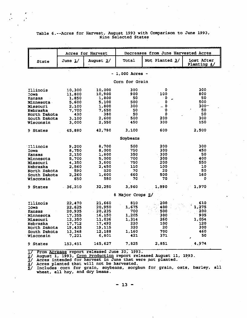
Table 6.--Acres for Harvest, August 1993 with Comparison to June 1993,Nine Selected States

Acres for Harvest Decreases.from June Harvested AcresState June 1./ August 2:./ Total Not Planted ~/ Lost After

Planting JJ

- 1,000 Acres -Corn for Grain

IllinoisIowaKansasMinnesotaMissouriNebraskaNorth DakotaSouth DakotaWisconsin9 States

.IllinoisIowaKansasMinnesotaMissouriNebraskaNorth DakotaSouth DakotaWisconsin9 States

IllinoisIowaKansas

.MinnesotaMissouriNebraskaNorth DakotaSouth DakotaWisconsin9 States

10,30011,8001,8505,6002,1007,700

4303,1003,000

45,880

9,2008,7502,1505,7004,3502,560

5902,260

65036,210

22,47022,62520,93517,35512,35017,71219,43513,3487,221

153,451

10,00010,9001,8005,1001,8007,650

3802,6002,550

42,780

8,7008,0001,8005,0003,6002,450

5201,600

58032,250

21,66020,95020,23516,15011,03617,49219,11512,1886,801

145,627

30090050

5003005050

500450

3,100Soybeans

50075035070075011070

66070

3,9608 Major Crops 2-./

8101,675

7001,2051,314

220320

1,160421

7,825

o100

oo

- 0·0o

200300600

20030030030020010020

50070

1,990

20040050030026010020

700371

2,851,

300800

50500300-5050

300150

2,500

30045050

4005501050

160o

1,970

6101,275

200905

·1,05412030046050

4,,9741./ From Acreaqe report released June 30, 1993.2/ August 1, 1993, Crop Production report released August 11, 1993.1/ Acres intended for harvest in June that were pot planted.~/ Acres planted that will not be harvested.2./ Includes·corn for grain, soybeans, sorghum for grain, oats, barley, all

wheat, all hay, and dry beans.

- 13 -

Imagery from two different satellite series is commonly used. Oneis information from the Advanced Very High Resolution Radiometers(AVHRR) aboard the NOAA weather satellites. These sensors have onevisible band and one near infrared band. Data from weathersatellites are very coarse with each data element, or pixel,representing about one square kilometer on the ground. The weathersatellite advantage is that observations are taken every day. Thenormal way of examining weather satellite data is to calculate aveqetati ve index from a ratio of the two bands of data. Much dataare lost each day due to clouds so the usual technique is toextract the highest noncloud readings for each data point and eachband across a 2-week period and use those values for calculations.The united states Geological Survey organization does create apicture product for the u.s. from the data sense~ every 2 weeks.During the 1993 qrowing season, NASS acquire~the AVHRR data-on ~priority basis, including the preliminary information for the firsttfeek of every 2 week period. NASS' developed -routines forprocessing the entire file on a Sun Sparc-2 work station andcreating map products at several different scales. Individuals inthe NASS Research Division also loaded the entire file of 1992AVHRR vegetative index data. Once that was done, a series ofbiweekly crop vegetative difference images was created which-compared 1993 conditions to 1992. Areas which were primarilynoncrop were masked as a neutral color and all other points wereclassified into five colors representimj "much-lower vegetativeindex" up to "much-higher vegetative index." Figure 5 illustratesin black and white the types of product that were created in colorduring the qrowing season.The vegetative difference imaqes were 'very helpful for a visualperspective on the extent of the flooded area and were of greatinterest to USDA policy officials. However, proper interpretationof them depended on a good understanding about previous growingseason conditions and it was not possible to convert information to .a yield per acre judgement •.The other siqnificant satellite ~ata source for agriculturepurposes is the Landsat series. The Landsat 5 which is still inorbit contains the Thematic Mapper (TM) sensor which collectsreflectance in seven different wavelengths. NASS was the earlyleader in developing procedures to process entire frames (about 100nautical miles on a side, containing 40 million data points in eachband) of digital satellite data. Proper utilization of Landsatdata requires samples of known ground data within each scene andprecise registration of satellite data points to the correct fieldson the qround. For the TM, each pixel represents 30 m~ters on theground so much more precise interpretations can be made than withAVHRR data. However, the repeat cycle of the satellite' is 16 daysand the sensor is very susceptible to cloud problems so manydesired agricultural targets are often missed during the peak partsof the growing season.

- 14 -

••. ..

Biweekly Crop Vegetation Index Difference for 1993 minus 1992

Period 20 (6/25 - 7/08) Period 24 (7/23 -. 8105)

Higher r~~~;~i~ilNon-Crop/Occasional Cropland• Lower. Same

..

NASS studies with Landsat have shown that cloud free images, whichare reasonably optimum in time of acquisition, yield relativeefficiencies of three or higher. That is, combining the satelliteclassifications with the area frame survey data used for trainingimproves precision of acreage estimates as much as if three timesas many ground observations were added.Landsat data do not' offer any timing benefits for NASS. NASSissued the Prospective Plantings report at the end of March and theAcreage report the end of June but the earliest time fordifferentiating corn from soybeans with Landsat data is mid to lateAugust. It is also not likely that Landsat data interpretation cantell corn silage fields from those for corn for grain ordifferentiate marginal corn fields that won't be harvested fromthose that will. ,...USB 01' CROP COIJDITIOIf DATAThe Weekly Weather Crop Survey, which monitors crop progress, alsocollects crop condition data from the panel of reporters. A fiveadjective scale of "excellent," "good," "fair," "poor," and "verypoor" is used for each crop. Those data are summarized each weekas weighted State averages. Each State is divided into

_Agricultural Statistics oistricts (ASO's) which are contiguousgroupings of counties in the State. Crop acreages within each ASOare used for weighting.Although NASS would caution individuals to not put much confidencein these condition data which come from such a small panel (usuallyless than 100 reporters per State or about 12 or fewer per ASO) ,weekly reports are closely followed •. Many people have creatednaive yield prediction models from the data series and NASS hasexplored the use of condition as one variable in early seasonmultiple regression models for wheat yield forecasting.Figures 6-9 illustrates a simple approach that assigns a numericvalue to each adjective to create a weighted State average index.The Iowa condition data about August-1 indicate an averaqe yield of100 bushels per acre when the actual forecast based on objective

.yield and grower supplied data was 115. About October 1, theindication of slightly below 100 bushels does more closely matchthe Iowa October 1 forecast of 105 bushels per acre. Figures 6 and7 indicate the Iowa final yield actually turned out to be only 80bushels per acre--more about the reasons for that later., Figures 8and 9 show that the Ohio corn crop condition did decline during theseason when drought was experienced. In this case, the August 1and October 1 conditions did indicate quite closely the officialforecasted levels for the two periods (128 and 113).

- 16 -

[ .

COMPARISON OF CROP CONDITIONS AND YIELDS 1/

Figure 6Iowa August Condition VB Corn Yield

BU8HELS PER ACRE180

Figure 7Iowa October Condition vs Corn Yield

BUSHEL8 PEA ACRE180

150

140

180

120

110

100

10eo70

115 17

13

11 21 23 H 27CROP WEATHER CONDITION INDEX

!lE 12

•

21

110

140

180

120

110

100

10

80

7011 17

••11 21 lIS IS 17

CROP WEATfER CONDlT1ONINDEX21

Figure 8Ohio August Condition vs Corn Yield

8U8HEL8 PER ACRE1110

Figure 9Ohio October Condition·vs Corn Yield

BU8HEL8 PER ACREtlO

·····140

7012 ~ 115 • 20 U ~ H 21 80

CROP WEATHER CONDITION INDEX

7012 ~ 115 • 10 U 2. H 21 80

CROP WEATHER CONDmON INDEX

1/ Based on Weekly Weather Crop Survey and Official Yield Estimates.

- 17-

YIBLD PORBCAST PROCBDURBSNASS maintains strict security procedures for all of its estimatingprograms to ensure that no one outside the Agency has access to anyinformation ahead of time. For monthly CrOD Production forecastsof the yields of corn, soybeans, wheat, cotton, and sweet oranges,additional'security procedures, which include total isolation ofthe staff which prepares final state and·U.S. forecasts, are used.One key feature is that a ·few leading producing States, whichusually make up about 80 percent of production, are specified asthe "speculative" States. The state Statistical Officerecommendations for those states cannot be examined except underlockup.conditions in the final hours as the current report is beingprepared. Some comparisons to follow in this paper are based ontotals or averages for these speculative states which are normallyall states which have objective yield survey~ Figures 10 aftd~1show the objective yield· States for corn and soybeans, 'along withthe limited forecast states and the "full forecast", States whichhave a grower survey each month.Yield indications that NASS receives are biased and the process instate statistical Offices and Agricultural Statistics Board (ASB)deliberations is aimed at interpreting the current amount of bias •.Reports of yield received from farmers during the growing seasonwill be biased on the low side of final yields. Farmers tend to beconservative in early season reporting since it is easy tovisualize the number of things that can happen in .the upcomingmonths before harvest to limit the final yield per acre. Thisamount of underreporting reduces each month. as the crop comescloser and closer to maturity. The survey indication from theDecember Agricultural Survey, when most harvest is completed, isusually at the final average yield level.Objective yield indications for yield are usually somewhat abovethe final average yield level. Objective yield procedures forecast .biological yield and it is not possible to account for allharvesting losses which is one reason for the bias. Another factoris that the objective yield interview process asks such detailed

.questions on acres in a field, acres planted in that field, acresnot now in production, etc., that the farmer's concept of theobjective yield field becomes smaller than they would report on amail or telephone inquiry. Thus, there may not be much biasbetween total production and objective yield Droduction,in a fieldbut the yield indication will have an upwards bias.since NASS conducts the same surveys each year, the past history ofeach month's indications compared to final State yield~ is used toadjust for biases. In recent years, a combination of time seriesdata plots and numeric calculations of these differences have beenused to be sure that State office statisticians are using the sameinterpretation approach as the ASB in Headquarters.

- 18 -

,.

'. I.

Figure 10 States in the Corn Forecasting Program

• Objective Yield States

• Full Forecast States

_ Umited Forecast States

Figure 11 States in the Soybeans Forecasting Program

• Objective Yield States

• Full Forecast States

• Umlted Forecast States

- 19 -

'.. 'I

The ASB meets the morning that the CrOD Production report is to bereleased to consider the yield for the speculative states. Yieldshave been adopted for all other states and are being held in lockedfiles. The encrypted state office recommendations have been storedin a safe until the work area is secured and an armed guard posted.The ASB for each crop.normally consists of about eight members withat least two from state offices. The ASB concentrates on adoptingthe region average yield. Both the farmer yield and the objectiveyield are probability surveys with greater precision at theregional level than the state level. All historic results andcurrent indications are properly weighted to the region.Each ASB member reviews and interprets the regional indications andpast relationships and determines their recommendation. The ASBChairperson openly polls the members an~ all can see- th~differences in interpretation, if any.' Differences are discussedand the Board preliminary target is set. The commoditystatistician for that crop and one or two other statisticians thenreview individual state indications and recommendations and "set"the state yields while the ASB moves to other crops. If theresulting weighted average regional yield is not within rounding ofthe target, the Board may be reconvened. However, this is rarely.needed •. OBJECTIVE YIBLD HODBLS

All NASS objective yield programs are designed to forecast thenumber of fruit (ears of corn, wheat heads, soybean pods, oranges,etc.) at harvest time and weight per fruit. In most cases, thenumber of fruit can be forecast well" ahead of harvest but anaccurate forecast of weight per fruit is often the limiting factor.NASS uses two types of forecasting model approaches. Traditionalforecasting models are based upon data from objective yield samples .for the past 5 years and they calculate a yield for ea~h currentsample. Data are limited to 5 years since cultural practices and

.seed quality are constantly changing and older data might not be asbeneficial for forecasting current characteristics. For instance,in the past 3 years, NASS has observed a much higher rate ofsoybean pod retention from pod forming to harvest, probably due tovarietal improvement.The other modelling approach examines past August and Septemberrelationships of individual components and combinations ofcomponents to determine those which are well correlated with finalyield. For example, september number of ears per acr~ multipliedby kernel row length is better correlated-with final yield than theaverage calculated yield of all samples from the traditionalapproach.

- 20 -

Monthly forecast models for corn and soybeans are based on uponmaturity stages. The corn stages are the biologic~l stages shownin Table 7. For soybeans, mOdelling is actually based on detailedmaturity categories which are determined from relationships amongvarious fruit counts. NASS research showed that relationshipsbetween early season fruit counts and final pods with beans variedgreatly depending upop exactly which maturity stage was observed onthe day of data collection. For example, since not all blooms onthe plant go on to form pods, there is a great difference in datarelationships when pods make up only 25 percent of the blooms andpods compared to when pods make up 75 percent. Some maturitycategories last only a few days so NASS uses a very small countunit in order to ~nsure accurate counts.

Table 7.--Corn Maturity Categories for Traditional For~cast MOdels

~=====c=o=d=e======:::I====================================D=e=f=i=n=i=t=i=o=n=============================~1

2

3

4

5

6

7

No ear shoots present.Pre-blister.--Little or no watery, clear liquid present inspikelets (unpollinated kernels) .Blister.--MOst spikelets have partially formed kernels that areenlarged and full of liquid~Milk.--MOst kernels are full of milk-like substance, but kernelsare not fully grown.Dough.--Kernels are full gro~. About one-half of kernelsshowing dent with some dough-like substance in all kernels.Dent. --Kernels are fully dented with no milk present in mostkernels. Kernels may be hard to scratch at surface.Mature.--Maturity line on the kernels at mid ear has advanceddown to the cob.

Forecast models are single variable regression equations of theform:

Y = a + bXwhere:Y = component to be forecasted,a = the intercept,b = regression coefficient for x,x = the independent variable from field counts or measurements.

21 -

., ),

Separate forecasts are calculated for number of ears per acre andaverage grain weight per ear. Table 8 lists the variables whichare used for each model, by maturity code.

Table 8.--Corn Forecasting MOdel Variables

I MaturityCode

Model 1 INumber of Ears

Model 2 I1

2-4

5-7

1-2

Number of StalksNumber of Stalks

Ears with kernelformation

Historic average

No modelStalks with ears or ear shoots tototal stalks; number of ears andear shoots ~/ .No model

Grain Weight per EarNo model

7

Average kernel row.lengthAverage field weight

Average length over .huskNo model

~/ Two different sub models are calculated and weighted together.

The traditional objective yield forecasting approach calculates ayield for each sample and averages all of the samples. AfterSeptember 1 and harvest of ears beqins the traditional forecastinqapproach and the new alternative procedures converqe. The finalobjective yield indication for each sample is based on actualcounts of fruit (ears, pods with beans, etc.) and actual weights.Before that time, the ASB process is improved by having.multipleindications to consider •.Use of this additional modelling approach, plus the graphinq ofearly season indications versus final weight or other'indications,has made Board members more coqnizant of factors that lead tohigher or lower fruit weights. This emphasis on studying yieldcomponents was a factor in improving forecasts in 1991 and 1992over the approach of only exa~ining the sample forecast averages.The objective yield models create very precise forecasts at theState and regional level. Coefficients 'of variation for averageyield or the yield components are usually 1 to 2 percent at theState level and 1 percent or less for the region. The coefficients

- 22 -

of variation are similar for the monthly ag yield survey. Thus,the sampling error is very small compared to the forecastina error.Since weather conditions can change tremendously between a monthlysurvey and the end of the season, the observed changes are muchhigher than the survey error. The easiest measure of forecasterror is the root mean square error of the monthly forecasts.Deviations from the ~onthly forecast to final yield are expressedas percentage changes. The average of the squared percentagedeviations for the past 20 years is presented in the reliabilitywriteup for each monthly publication. For corn, the root meansquare errors in 1993 were: August, 7.6 percent; September, 4.7;Oc;:tober,3.6;. and November, 2.4. For soybeans, the root meansquare errors were: August, 6.0; September, 5.3; October, 4.0, andNovember, 2.9.AUGUST 1 YIELD J'ORBCASTSThe August 1 data from the farmer surveys and objective yieldobservations pointed to an extreme mixture of yield potentials.Plant population and projected corn ears per acre were very highfor most objective yield States. The States of Illinois andIndiana had tremendous increases in soybean plants per acre from asignificant move to narrower row·planti~gs. Iowa corn yield was.forecast to be down 32 bushels from the record yield of 1992.However, Illinois and Indiana were both forecast at 140 bushels peracre, down only 9 and 7 bushels, respectively,. from their 1992records. The u.S. production forecasts of 7.42 billion bushels forcorn and 1.90 billion bushels for soybeans were fairly well in linewith the production levels of 1989-1991. Both figures were downfrom trend yield projections that the World Agricultural OutlookBoard had made in JUly using June Acreaae data and consideration ofvarious trend and weather models.One interesting agriculture phenomenon in recent years is that onenews service publishes a number of market analysts' estimates two .days or so ahead of major NASS reports. with rare exceptions,these analysts, from commodity trading firms or advisorY services,do not have any survey data but use prior government reports,

.weather, and market interpretations. The average of these figuresprobably does represent the general expectation of the "industry"ahead of a report. These "guesstimates" in August averaged 7.51and 1.86 billion bushels with respective ranges of 6.96 to 7.79 and1.75 to 1.90. Thus, the NASS soybean forecast was somevhat higherthan expected, probably due to high pod counts in the ObjectiveYield Survey.Forecasted production levels were down 22 percent for ,corn and 13percent for soybeans from 1992. After the Crop Production reportwas published and absorbed, there was an acceptance of thoselevels , given that normal weather might occur the rest of thegrowing season.

- 23 -

..

SBPTEllBER AND OCTOBER FORECASTSThere wasn't' anything normal about the 1993 season. There was aseason long drought in the Southeast States that greatly reducedyield potentials and caused some abandonment of corn acreage. Thedrought conditions spread into Ohio which had started with verygood yield prospects. The Ohio yield forecast went from 128bushels per acre in August to 115 in September.The objective yield counts continued to support the very high earcounts and projected pods per acre from August. The pods counts,however, were mixed between States. In 'the September 1 survey,Illinois and Indiana had pod counts 14 and 20 percent above theirprevious record levels, respectively, due to the adequate moistureand high plant populations. However, Iowa and Minnesota had podcounts equal to and 13 percent lower, respectively, than ~heirprevious low counts during the 1988 drought year. -A new factor in September and October forecasts was additionalspeculation about the amount of corn acreage for harvest. One,1993Feed Grain Program provision was referred to as "0-92." This meantthat a person who had a corn acreage base could sign up and plantno corn at all and still get 92 percent of maximum program

,paYments. Because of the flood, farmers were given an extension ofthe time period for enrolling in 0-92. The final date hadoriginally been April 30 but subsequent exten,sions allowed farmersto make decisions as late as September 17 if they had siqned up forregular provisions by April 30. This caused concern that a sizableportion of acreage might be destroyed and NASS forecasted acreagesfor harvest at grain might be too high.There also was a scare in Illinoi~ when articles were written aboutSudden Death SYndrome which was reported to affect and quickly killentire fields of soybeans. There are scattered disease, insect,hail, and other problems each year. The forecasted soybean acreagefor harvest for each State provides for abandonment due to thosefactors. The end-of-season surveys for Illinois did not show anydrop in soybean harvested acres over what NASS had alreadyforecast.NASS did keep the questions on acreage intended for harvest on themonthly ag yield survey each month instead of dropping them afterAugust. There were some small adjustments in the Octoger report:Minnesota corn acreage for grain harvest was lowered 500,000, Iowa100,000, and Missouri, Nebraska, and South Dakota 50,000 each.Each monthly survey, while supporting the acreage levels, did showlower and lower yieldS. In addition to the corn crop"being laterthan average, pollination was not good and kernel row lengths ofears were shorter than average. These shorter kernel rows providedindications by October 1 of Iowa and Minnesota ear weights nearlyas low as the drought years of 1983 and 1988.

- 24 -

'.

Figures 12-15 illustrate some of the information available from themonthly Objective Yield Survey. Figure 12 depicts the September 1linear relationship between a yield "proxy" (number of ears peracre multiplied by averaqe kernel row lenqth) and the final yieldin earlier years.Figure 13 depicts a ~esponse surface of yield projected onto thedistribution of numbers of ears and lenqth of ears. The responsesurface is shown as contour lines for various yield levels (100bushels per acre, 110 bushels per acre, etc.). Figure 13illustrates that the hiqh ear counts in 1993 provided the potentialfor more than an 110 bushel per acre averaqe, even with the shortaveraqe kernel lenqth.Figures 14 and 15 compare ears per acre available~weiqht data, andyield projections in October and November. _Fiqure 15 indieat~sthat the averaqe weiqht has come down almost 10 percent fromOctober and indicates an averaqe yield only siqh~ly above 100bushels per acre.Fiqures 16-19 present comparable relationships for Iowa. Fiqures 17and 18 illustrate that the yield potential based on averaqe kernelrow lenqth and the weiqhts from the earliest harvested samples was

.in the 105 to 112 bushel per acre ranqe. However, Fiqure 19indicates that, after an early October frost, the potential droppedto the low 80's. - .IJOVBKBBR 1 Y:IBLD PORBCASTSThe 1993 qrowinq season came to a sudden conclusion in earlyOctober. Killinq frost occurred in Minnesota, Northern Iowa, SouthDakota, and Wisconsin October 2 and 3 and moved across most of theCorn Belt by mid-October.Once frost has occurred, the moisture content of corn kernels and .soybeans usually drops quickly, allowinq harvest to occur. By theend of October, 50 percent of the corn acreaqe and 80 'percent ofthe soybean acreaqe had been harvested.In much of the flood affected area, farmers were shocked with theiractual corn yields. Kernel weiqhts were much lower than normalwith resultant drops in yield. A bushel of corn is defined as 56pounds at 15.5 percent moisture •. Crops are sold on a,weiqht andmoisture basis. Price is normally discounted for low test weiqhtand for every percent moisture above a standard. The yielddeclines from expectations were particularly severe in Iowa.Soybean yields in Iowa also turned out lower than farmers hadanticipated.

- 25 -

FIgure 12. - - CoInpIrtaon or Sepeem"" 1 Corn OY Indlcdona to FIneI YIeld

140

130

120ASB

Y 110I

•Id

100

90

80

110000 120000 130000

ICiM'neI LMIgth •

83•

•

160000

"'''',-"' ...'-..." ...

"' ...'-," "'," " " ....•..... '''•....

" " " ' •..",'..."'," "" •..

" '•.." •..'" " "',

"' •.." ' ...

"',' ...

-- 130-- 1201109080

88*

18813

81*

80•

83*

ASS Yield

" " ",.•••.•.....•....

"," ",

" ",.•..•..•...

" " ",....•.•...'" " " "

'" ".'"

'" " ",".5.95

18308

7.38

• 7.D1•Pt

1

L 6.65•n••th

In 6.30

26

"CompeI18onor 0c:II0ber, Corn OY Ind1cdona

•

......••..••••.•..•..•.•....

--"'"...•.........................

'...........•.........•.

" '...,.•.••.'."••........••.•...•..•..•.••

92*

130--- 120110

20884

Oct, .....,Acre10090

88•

18506

80ASB Yield

0.3346

0.2374

18147

0 0.8103ct

1

W• 0.2880I

••"tIb 0.2617

~~..~SO'..••.•..-

..••..•.. ~..~..........~..•..•....~~...•..•...••~..............~..~~.•....~~~~......~....~..~~~~"-~~....~..~~~~..•.~~~..•.~~..•.~~~..•.-~....~..~~~~~-....

•.•.•...•.

'-',.,.....,-..-, .•..•..•...

'-....••.•..•.....•.•...........•.

~ _- - ..•..•..•....•......•..........

-- 140-- 130

8S*

-- 120

20848Nov 1 .....,~

100 11090

19480

80Ase Yield

0.841

0.240

18113

N 0.818

0V

1

W• 0.281I

••ht

Ib 0.288

27

Figure 18. - - c:omp.teon of •••••••••. 1 Com OY IncDcatlone to FI••• YIeld - Iowa

150

140

130

A8B 120

YI

• 110Id

100

80

80

120000 1SOOOO

88•180000 170000

ComperIeon of Septem ••••. 1 Com OY IndIc 1110.-. - Iowa7.53

-........,-,80 ". "

" ". "" " " " " " '.•...

.•......... .•....•....•...

.•..•Dt....* .

.•....•....•........

.•.....................

.......•...............

................

.•.........

'". ,'.•.....' .........•....................•.....'...•...•...• •.....••....•.....'..••..•.....••........••.... ..,....•.........•••.........•.•....•••....•.....••....

-- 14-0-- 130

93x

-- 120

21834

8epI1 """'AcN100 11090

20248

80

83*

" "," ....•..•..•.

" ...•••...." .••..•..•.

" " .....•...." " .•..•.•.••.••.

","

.•.~...•..•......88 "* "", ...••.•.....•..

ASS Yield

5..94

18882

8 7.13•Pt

1

L 8.74•n••th

In 8.34

28

t.

I=Igurw 18. - - Com...,won of October , CoIn OY Indicationa - __0.367

0 0.324

ct

1

W• 0.282IIIIIt

IIt 0.280

0.22818888

ASB Yield 80 90

21470

Oct , EarWAa.

100 110 --- , 20 -- 130 --140

FIgww,8. - - CompIIrI8On of Novwnber , Corn OY •••• c••• a••• - Iowa

~ -~------. ---.---- ------------. ------------ .------.------.. ~---- ~ ~ --~~ ----- __ • 85~ "'- -------.:...

-- -- __ 82 • ------ "lr_ ~ _

-- ----'---- '--""--..-.--. 8t-.......... __-- '""-.-- * ~....._- ---... 84 ~

.••..----- -....-....~--- ......•.......~-- --'"""-,. ------------ ...•._- -------------... -----'""'----.

-- --------------------------------------- •......'------~------------- ..---..----.-- -------..........•. -

~ ---- - ---~----.•............•...•.......................•... --------- ..•..• --...... - ...•... ---- .......•... :.:.----".---.

CI'Q - ••••.'"* --~---..._----'.

0.371

N 0.3310y

1

W

• 0.280IIIIIt

IIt 0.248

0.20818870

ASB Yield 80120

21446Nov, ....."Aa.

90130

100140

110ISO

29

.-

For the u.s. as a whole, the decrease in corn yield potential fromOctober 1 to November 1 was larqer than any experienced in the past20 years. Table 9 presents the October to November comparison forboth corn and soybeans. The 20 bushel per acre drop in Iowa wasclose to the absolute record for that state in any month.

Table 9.--Comparison of 1992 and 1993 U.S. Production ForecastChanges from October 1 to November 1 with Recent History

Change inCrop and Comparison Yield Per Acre I Production

Bushels Mil. Bu.Corn

Largest change 1972-1991 +2.8 +198Change in 1992 +5.5 +391Change in 1993 -7.2 -459

SoybeansLargest change 1972-1991 +1.4 +81Change in 1992 +1.0 +59Change in 1993 -1.0 -57

D1D OF SBASO. YIBLD BSTDlATBSAs farmers completed their harvest, many found final yield turnedout to be even lower than experienced with their early harvest.For example, the end-of-season corn yield estimate for Iowa , based .on the December Aqricultural Survey, was another 5 bushels lowerthan November. The corn yields in Iowa and Minnesota ended uplower than durinq the 1983 and 1988 drouqht years.soybean yields were not as adversely affected as for- corn andIllinois and Indiana did realize the hiqh potential which had beenpresent all season. Table 10 presents the 1993 chanqes for eachmonth to the final compared with other years.

- 30 -

", .

Table 10.--Comparison of Changes in u.s. Production Forecastto the End of the Season, 1992, 1993, and Historic Maximums

Month RMSE 1/ Maximum Change Change in Change in1972 - 1991 1992 1993

- - - - - - Million Bushels - - - - - -Corn

August 1,192 -1,063 +720 -1,079September 719 +660 +712 -885October 563 +538 +544 -618November 401 +378 +153 -159

SoybeansAugust 212 -207 +109 -93September 186 -124 +103 . -101October 143 +120 +80 -82November 119 -109 +21 -25

1/ 90 percent confidence interval for root mean square error calculation basedon 1972-1991 results.

WHY WEREN'T EARLY FORECASTS CLOSER TO FINAL YIELD? Looking back atthe NASS historic performance record, it is easy to assume thatforecasts should have been closer to final estimates. Prices rosesignificantly after the November forecasts but some people hadalready sold much of their crop on contract before the price rise.There was surprisingly little reaction from farmers at the time ofthe November forecasts since theY,hadn't been able to determinetheir own low yields until harvest.There were at least four theories expressed for the drastically lowyields in States like Iowa, Minnesota, and South Dakota. Thoseare: (1.) excess moisture caused significant leaching out ofnitrogen, (2) there were not enough growing degree days in 1.993,(3) timing of frost prevented final accumulation of dry matter incorn kernels, and (4) "the crop just quit" even before frost.Concern about nitrogen leaching was mentioned throughout theseason, once soil conditions became so saturated. Corn depends onextracting nitrogen from the soil; soybean plants actually returnnitrogen to the soil so they would not be affected. No definitivestudies on 1.993 effects of nitrogen leaching are known but cornfarmers are being encouraged to apply additional nitrogen in 1.994since soil levels are believed to be lower than normal.' Individualfarmers can run soil tests to determine their 1.994 needs.

- 31. -

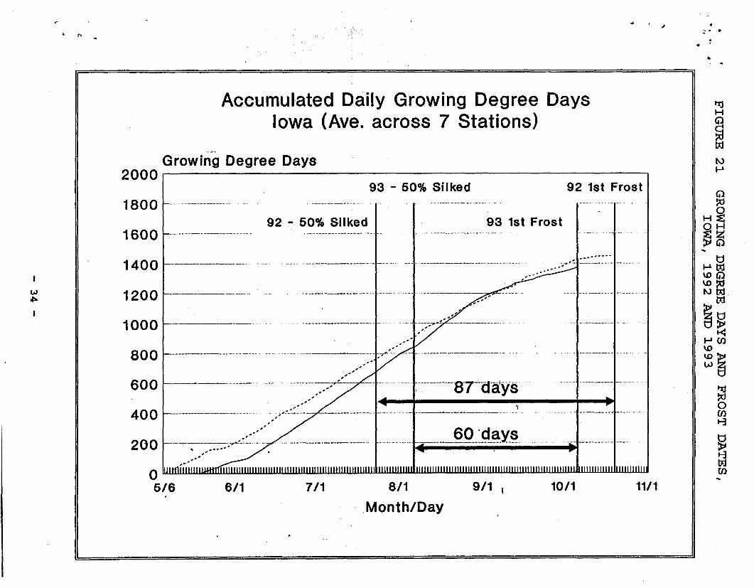
The 1993 season was cool and people might conclude that growingdegree days could be a significant factor in lowering corn yields.(Growing degree days accumulate the daily maximum temperaturesabove 50°F, with an upper cutoff of 85°F, if the daily minimum is50°F or higher.) Soybean plants react more to length of day fortriggering of growth stages so they would be less affected bygrowing degree days •. Figure 20 shows the growing degrees days forIowa in the past three seasons, with accumulation starting at April1. This does indicate that 1993 was considerably lower than 1991for total growing degree days but was higher than 1992 which wasthe record producing year. Thus, lower growing degree days is notthe single contributing factor.The greatest contributor to the lower yields in Iowa, Minnesota,and South Dakota was corn crop maturity at the time of the killingfrost •. Figure 21 expresses several comparisons of the 199~ and1993 Iowa seasons. In this graph, growing degree days have beenaccumulated from the 4ate that 50 percent of the corn crop wasplanted. This illustrates that the 1993 growing degree days didtrail 1992 until mid-August. Thus, corn was affected both by laterplantings and cooler temperatures. One commonly accepted "rule"for corn production is that it takes 60 days from pollination tomaturity. Figure 21 indicates that the 1992 corn crop in Iowa had·87 days from the 50 percent silking date to first frost. However,in 1993, there were 60 days from the 50 percent silking date tofirst frost so only about 50 percent of the crop would have reachedbiological maturity. Frost was not early but the crop was notready for this nearly normal frost date.Figures 22 to 25 illustrate the effects of the lower than expectedear weights. Figure 22, based on data from all objective yieldstates, shows that the regional average was about 5 percent lowerthan would be expected from previous years. Figure 24 shows thatthe average weight in Iowa was more than 10 percent lower. Thesame type of discrepancy would be true also in Minnesota, South .Dakota, and Wisconsin. Figures 23 and 25 indicate that average earweights in Indiana and Ohio were about 10 percent higher thanexpected based on the shorter than average ears.Lack of time from silking to frost is surely the largestexplanation and is likely what people mean when they feel the "cropquit." However, higher moisture conditions and early cool weatherprobably did lead to some additional disease problems and to plantsand fields which did not look healthy and normal. Thus, somepeople concluded that the plants just wore out by October 1.

- 32 -

. .,

Growing Degree Days2500

Accumulated Daily Growing Degree DaysIowa (Ave. across 7 Stations)

..-......,,,,,,,,_____ •__ ._._ •••r•••·•..- ••••M. __ •••••••••• _ •• , ••••• ·• •• · ••• _ •••• ··,,,· .--. •••••• __ ••••••••••••• _. __ ••••••••••••••••••••••••••.••••••••••.•••••• - •••••••••••••••••••• -.'-.-.---- -._-

"","",

""",,.,,,,:::-;.-...""" .." ....",,- -"""""."._-_._"--"_." .._"-"."._,, .. ,,,, """."." .... " ... " .".. "". "" ....,.""""""""""."""." .". "",,-,,"' .. ".

"",,,

",,'-,

~. .,

ITjH

~tJ;j

t.J0

(j)::0

~H

~

t1tJ;j(j)::0tJ;jtJ;j

~.to<{fl

HZH

~)i...•.....\D\D•.....I

•.....\D\DLV

11/1

........................ , ." .., ...-.--....'

.-..-." .., - -.., ...•...•..•......•......•. ,.•.." ...•..•.••......- - -- ".--- ......•..•.".......•..................................................... "...- -- "..•..•.... ,.•....... "..""

7/1 8/1 9/1 I 10/1

Month/Day6/15/1

1993

.mn 1991

- 1992

..

o. 411

500

1000

1500

2000

• •'>

... " •::..•

... .

92 1st Frost

10/1 11/1

93 1st Frost

9/1 I

93 - 50% Silked

8/1

Month/Day

-- -_ •••••••••••••••••••• m : •••••••••• --.- •••••• STdays ..

7/1

92 - 50ero Silked

6/1

..',.'......_ . :.;.'n" _.. ~__ .. '.' .~H ' •••• _", •••• " ,,._,,· •••••• ~_.·.··_·

,,,

... . ....•.•. ~:~.m :' __ __ .__ .__ _ _ m __ §.O_~d~_Y~..mmm, " ..'

",.

o5/6.

Accumulated Daily Growing Degree DaysIowa (Ave. across 7 Stations)

18001600140012001000800

600

400200

.~-Growing Degree Days

2000

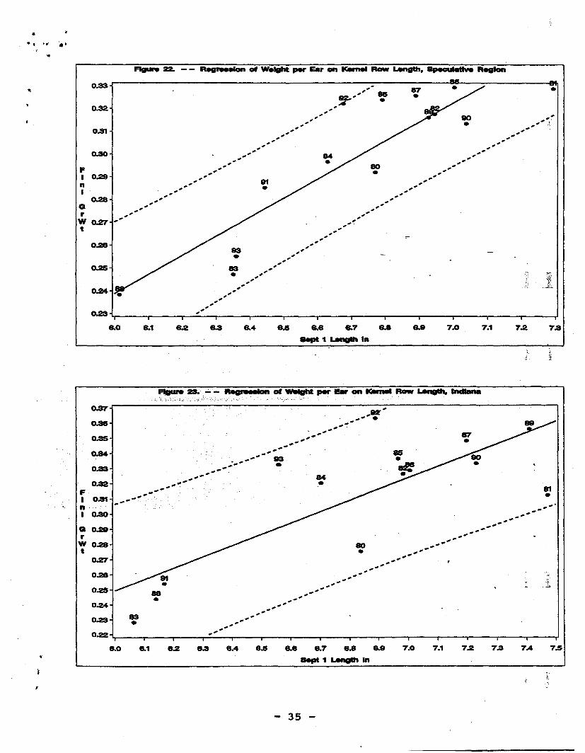
FIgure 22. -- Regr ••• 1on or Weight per Ear on ~ Row 1AnSIth. ap.~ Region

..... ,t~, '.'..

0.33..,

0.32

0.31

o.soFI 0.29nI

0.28GrW 0.27t

0.28

0.26

0.24

0.23

•

86•87• •

8.0 8.1 8.4 8.6 8.8 8.7 8..

Sept, ••••••• In7.0 7.1 7.2 7.3

.','., ......',,..",........,....'

.. "._,- 88,.....'.... ,

••" •• 84..' .,........'........

83•

88•

r i.

87•

81•,. ---- ................••.....••......

80 ••••••'... ,,,...••.............••......................................................,..8.0 8.1 8.2 8.3 8.4 8.5 8.8 8.7 8.8 8.9

Sept 1 ••••••• In

35

7.0 7.1 7.2 7.3 7A 7.5

FIgUre 24. - - Fe••••• 'on of Weight per Ear on KM'neI Row •.••••••• Iowe

- ....--'"......-,,",,",,---,,-..-,,".."..",

-",-"...",,'",•....

,",,",,-.."..",,",,".......•.-',

-,,'"..."_ ...-...•...•.......•.......

0.35~0.34

0.33

0.32

0.31

0.30

F 0.28In 0.28I

0.27Gr 0.28

Wt 0.25

0.24

0.23

0.22

0.21

0.20 83•0••

8.0 8.1

81•

88•

86•89•

8.8 8.7 8.8 8.9

Sept , ••••••• In7.0

88•

7.1 7.2 7..4

81•

-'-----"------....,,"..-... '"-....-...---......--.....",,-....-...----"••••113....•..-....•....

•••••.••• I0Il of WeIght JMlI' Ear on ~ Raw a..natb. Ohio

88•

7.17.0

82•

80•

8.8

85•84•

81•

82•

8.5 8.8 8.7

Sept 1 ••••••• In

8.4

8S•

........-".........•.

-"-""....

",";,.-~",",,' ,..--..

-'"-"..... ,--'----...--------- ..

0.28 81•0.25

0.24 88•0.23

8.0 8.1

o.ss

0.34

0.33

0.32

0.31FI 0.30nI

0.28G

r 0.28Wt

0.27

36

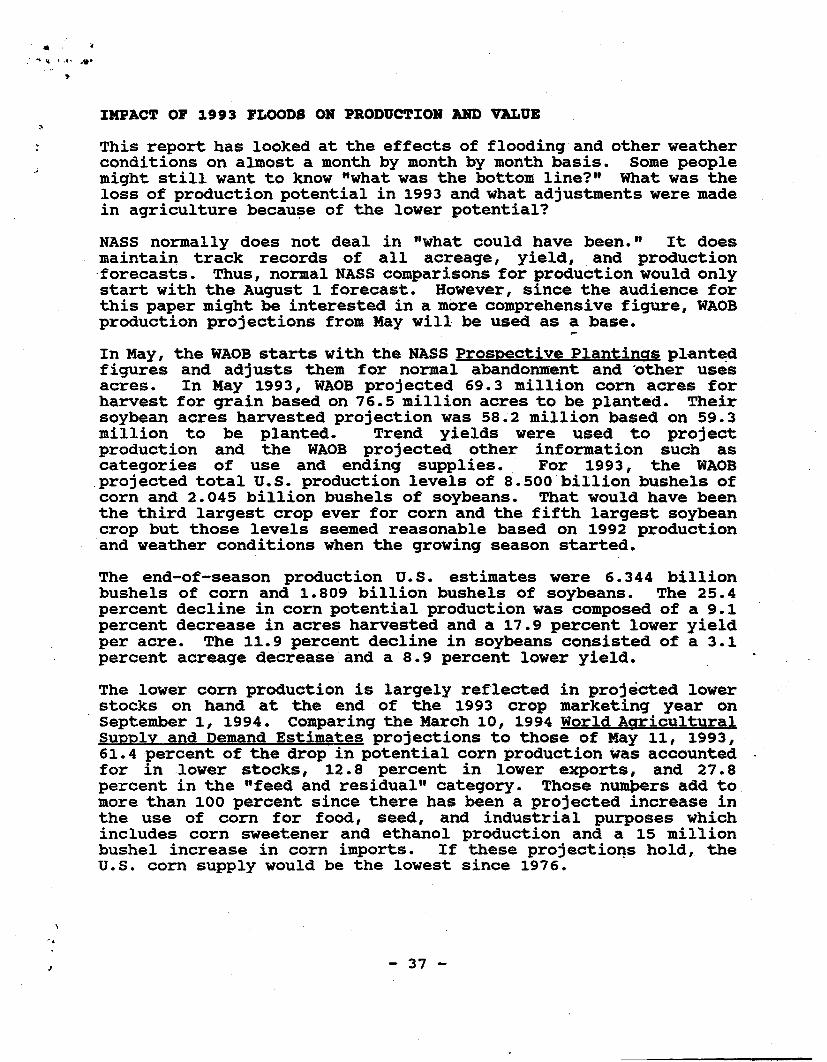
IMPACT OF 1993 FLOODS ON PRODUCTION AND VALUBThis report has looked at the effects of flooding and other weatherconditions on almost a month by month by month basis. Some peoplemight still want to know "what was the bottom line?" What was theloss of production potential in 1993 and what adjustments were madein agriculture becau~e of the lower potential?NASS normally does not deal in "what could have been." It doesmaintain track records of all acreage, yield, and production-forecasts. Thus, normal NASS comparisons for production would onlystart with the August 1 forecast. However, since the audience forthis paper might be interested in a more comprehensive fiqure, WAOBproduction projections from May will be used as a base.In May, the WAOB starts with the NASS ProsDective Plantinas plant~dfigures and adjusts them for normal abandonment and 'other usesacres. In May 1993, WAOB projected 69.3 million corn acres forharvest for grain based on 76.5 million acres to be planted. Theirsoybean acres harvested projection was 58.2 million based on 59.3million to be planted. Trend yields were used to projectproduction and the WAOB projected other information such ascategories of use and ending supplies. For 1993, the WAOB

_projected total u.s. production levels of 8.500 billion bushels ofcorn and 2.045 billion bushels of soybeans. That would have beenthe third largest crop ever for corn and the fifth largest soybeancrop but those levels seemed reasonable based on 1992 productionand weather conditions when the growing season started.The end-of-season production U.S. estimates were 6.344 billionbushels of corn and 1.809 billion bushels of soybeans. The 25.4percent decline in corn potential production was composed of a 9.1percent decrease in acres harvested and a 17.9 percent lower yieldper acre. The 11.9 percent decline in soybeans consisted of a 3.1percent acreage decrease and a 8.9 percent lower yield.The lower corn production is largely reflected in projected lowerstocks on hand at the end of the 1993 crop marketing year onseptember 1, 1994. Comparing the March 10, 1994 World AgriculturalSupplv and Demand Estimates projections to those of May 11, 1993,61.4 percent of the drop in potential corn production was accountedfor in lower stocks, 12.8 percent in lower exports, and 27.8percent in the "feed and residual" category. Those nUlllPersadd tomore than 100 percent since there has been a projected increase inthe use of corn for food, seed, and industrial purposes whichincludes corn sweetener and ethanol prOduction and a 15 millionbushel increase in corn imports. If these projectio~s hold, theu.s. corn supply would be the lowest since 1976.

J - 37 -

.~~\. ..• .• " .iI', .~

III

1

One other aspect of the monthly WAOB report is projection ofaverage farm price. Between May 1993 and March 1994, theprojection has changed from $2.05 per bushel to $2.60. As aresult, the projected value of the crop has declined only 5.3percent in spite of the 25.4 percent decline in production. Thus,the decline in value to the corn producing sector was small but theeffect was very severe for producers who had small crops.PROCEDURES POR THE PUTURE

All in all, NASS was pleased with the efforts undertaken in 1993.The Agency was able to gear up on short notice to add questions,edits, and summary routines in time for the August 1 and latersurveys. Some lessons were learned which would make thoseprocesses even smoother if such an emergency resurfaces.The procedures for evaluating acreage not· planted' and acresremaining to be harvested by August 1 worked very well. The end-of-season adjustments of planted acreage after the DecemberAgricultural Survey were only 0.5 percent for corn and 0.2 percentfor soybeans. Similarly, the end-of-season harvested acreage forsoybeans ended up only 0.2 percent higher than forecast in August.The corn acreage actually harvested for grain was down 1.5 percent

.from August, largely accounted for by October 1 when the 0-92signup had been completed.The yield forecasting approach of focusing on individual compon~ntsinstead of just the composite yields was very helpful in 1993. Itallowed NASS staff members to reference the high plant and earcounts for corn and the record high pod counts in some States inanswering questions during the season.' NASS publishes selectedobjective yield survey counts each year in the November CropProduction report. Some data users have now requested that theAgency publish monthly its assumed fruit counts and weights forcorn and soybeans. That request will be considered.The graph of days from silking to frost for Iowa illustrated thebiggest shortcoming in 1993 forecasts. No weather models areavailable which absolutely predict the date and severity of firstfrost.One change that NASS is making for 1994 is to select samples ofears which have reached the dent stage in the September 1 andOctober 1 Objective Yield Surveys for laboratory analysis.(Normally ears are not sent in until the mature stage unless thefarm operator is going to harvest at a high moisture level.) .Oneagronomy theory is that 90 percent of the kernel weight has formedby the dent stage although there is some disagreement from othercorn researchers. Sampling the dent stage ears will allow theAgency to determine if final weight per ear can be predictedearlier.

- 38 -