arX

iv:1

209.

4110

v1 [

mat

h.N

T]

18

Sep

2012

THE ZAGIER MODIFICATION OF BERNOULLI NUMBERS

AND A POLYNOMIAL EXTENSION. PART I.

ATUL DIXIT, VICTOR H. MOLL, AND CHRISTOPHE VIGNAT

Abstract. The modified

B∗

n=

n∑

r=0

(n+ r

2r

) Br

n+ r, n > 0

introduced by D. Zagier in 1998 are extended to the polynomial case by replac-ing Br by the Bernoulli polynomials Br(x). Properties of these new polyno-mials are established using the umbral method as well as classical techniques.The values of x that yield periodic subsequences B∗

2n+1(x) are classified. The

strange 6-periodicity of B∗

2n+1, established by Zagier, is explained by exhibit-

ing a decomposition of this sequence as the sum of two parts with periods

2 and 3, respectively. Similar results for modifications of Euler numbers arestated.

1. Introduction

The Bernoulli numbers Bn, defined by the generating function

(1.1)t

et − 1=

∞∑

n=0

Bntn

n!

are rational numbers with B2n+1 = 0 for n ≥ 1 and B1 = − 12 . The sequence {Bn}

has remarkable properties and it appears in a variety of mathematical problems.Examples of such include the fact that the Riemann zeta function

(1.2) ζ(s) =

∞∑

n=1

1

ns

evaluated at an even positive integer s = 2n is a rational multiple of π2n, the factorbeing

(1.3)ζ(2n)

π2n=

22n−1

(2n)!(−1)n−1B2n.

Their denominators are completely determined by the von Staudt-Clausen theorem:the denominator of B2n is the product of all primes p such that p − 1 divides 2n(see [11] for an elementary proof). It is often the numerators of B2n that arethe objects of interest. It is a remarkable mystery that there is no elementaryformula associated to them. These numerators appear in connection to Fermat’slast theorem (see [14]) and also in relation to the group of smooth structures onn-spheres (see [9], page 530 and [10] for details).

Date: September 20, 2012.1991 Mathematics Subject Classification. Primary 11B68, 33C45.Key words and phrases. Bernoulli polynomials, Chebyshev polynomials, umbral method, pe-

riodic sequences, Euler polynomials, generating functions, WZ-method.

1

2 A. DIXIT, V. H. MOLL, AND C. VIGNAT

D. Zagier [21] introduced the modified Bernoulli numbers

(1.4) B∗

n =

n∑

r=0

(

n+ r

2r

)

Br

n+ r, n > 0

and established the following amusing variant of B2n+1 = 0:

Theorem 1.1. The sequence B∗

2n+1 is periodic of period 6 with values

{ 34 ,− 1

4 , − 14 ,

14 ,

14 , − 3

4}.One of the goals of this work is to extend this result to the polynomial

(1.5) B∗

n(x) =

n∑

r=0

(

n+ r

2r

)

Br(x)

n+ r, n > 0

which is defined here as the Zagier polynomial. Here Br(x) is the classical Bernoullipolynomial defined by the generating function

(1.6)text

et − 1=

∞∑

n=0

Bn(x)tn

n!.

The objective of the paper is to produce analogues of standard results for Bn(x)for the Zagier polynomials B∗

n(x). For example, a generating function for thesepolynomials appears in Theorem 5.1 as

(1.7)

∞∑

n=1

B∗

n(x)zn = −1

2log z − 1

2ψ (z + 1/z − 1− x)

where ψ(x) = Γ′(x)/Γ(x) is the digamma function. The generating function (1.7)really corresponds to the less elementary expression

(1.8)∞∑

n=0

Bn(x)zn =

1

zζ(2, 1/z − x+ 1).

Here ζ(s, a) is the Hurwitz zeta function, defined by

(1.9) ζ(s, a) =∞∑

n=0

1

(n+ a)s.

A derivation of (1.8) is given in Section 5. The next example corresponds to thederivative rule B′

n(x) = nBn−1(x) for the Bernoulli polynomials. It appears inTheorem 8.2 as

d

dxB∗

n(x) =

⌊n

2⌋

∑

j=1

(2j − 1)B∗

2j−1(x) for n even

and

d

dxB∗

n(x) =1

2+

⌊n

2⌋

∑

j=1

2jB∗

2j(x) for n odd.

Finally, the analogue of the symmetry relation Bn(1 − x) = (−1)nBn(x) is estab-lished as

(1.10) B∗

n(−x− 3) = (−1)nB∗

n(x).

This is the content of Theorem 11.1.

ZAGIER POLYNOMIALS. PART I. 3

The original motivating factor for this work was to extend Theorem 1.1 to othervalues of B∗

2n+1(x). The main result presented here is a classification of the valuesx ∈ R for which B∗

2n+1(x) is a periodic sequence, Zagier’s case being x = 0.

Theorem 1.2. Assume {B∗

2n+1(x)} is a periodic sequence. Then x ∈ {−3, −2, −1, 0}or x = − 3

2 where B∗

2n+1

(

− 32

)

= 0.

In the case of even degree, the natural result is expressed in terms of the differenceA∗

2n(x) = B∗

2n(x) −B∗

2n(−1).

Theorem 1.3. Assume {A∗

2n(x)} is a periodic sequence. Then x ∈ {−1, 0, 1, 2}.The period is 3 for x = −1 and x = 2 while A∗

2n(x) vanishes identically for x = 0and x = 1.

An outline of the paper is given next. Section 2 contains a basic introductionto the umbral calculus with a special emphasis on the operational rules for theBernoulli umbra. Section 3 gives the generating function of the modified Bernoullinumbers B∗

n and this is used to give a proof of the 6-periodicity of B∗

2n+1. Aninversion formula expressing Bn in terms of B∗

n is given in Section 4. The proofextends to the polynomial case. The generating function for the Zagier polynomialB∗

n(x) is established in Section 5 and an introduction to the arithmetic propertiesof special values of these polynomials appears in Section 6. Expressions for thederivatives of the Zagier polynomials are given in Section 8. Some binomials sumsemployed in the proof of these results are given in Section 7. The basic propertiesof Chebyshev polynomials are reviewed in Section 9 and used in Section 10 to givea representation of the Zagier polynomials in terms of Bernoulli and Chebyshevpolynomials and also to prove a symmetry property of B∗

n(x) in Section 11. Section12 contains one of the main results: the classification of all periodic sequences ofthe form B∗

2n+1(x). This result extends the original theorem of D. Zagier on the6-periodicity of B∗

2n+1. Several additional properties of the Zagier polynomials arestated in Section 13. The results discussed in the present paper can be extendedwithout difficulty to the case of Euler polynomials. These extensions are statedin Section 14 and used in Section 15 to establish a duplication formula for Zagierpolynomials.

2. The umbral calculus

In the classical umbral calculus, as introduced by J. Blissard [1], the terms an ofa sequence are formally replaced by the powers an of a new variable a, named theumbra of the sequence {an}. The original sequence is recovered by the evaluationmap

(2.1) eval {an} = an.

The introduction of an umbra for {an} requires a constitutive equation that reflectsthe properties of the original sequence. These ideas are illustrated with the umbraB of the Bernoulli numbers {Bn}.

An alternative approach to (1.1), as a definition for the Bernoulli numbers Bn,is to use the equivalent recursion formula

(2.2)

n−1∑

k=0

(

n

k

)

Bk = 0, for n > 1,

4 A. DIXIT, V. H. MOLL, AND C. VIGNAT

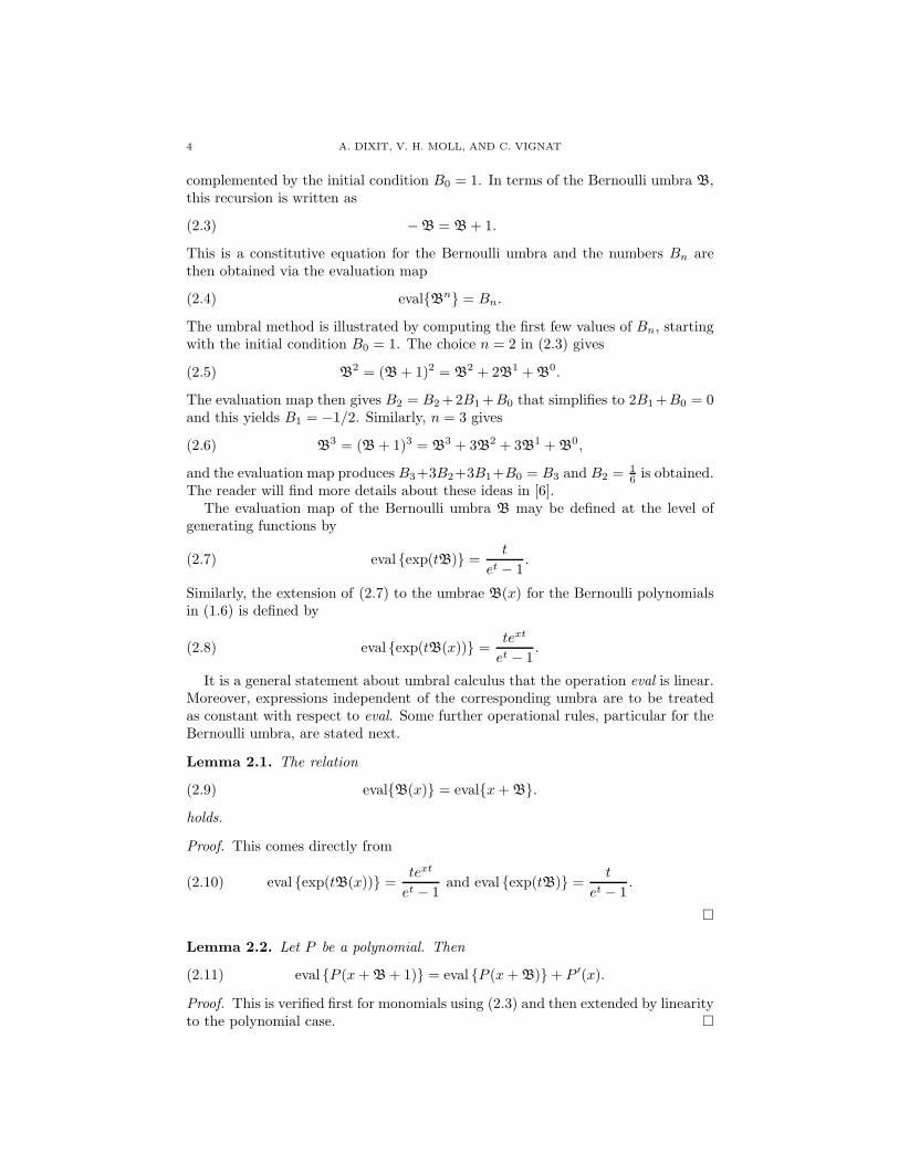
complemented by the initial condition B0 = 1. In terms of the Bernoulli umbra B,this recursion is written as

(2.3) −B = B+ 1.

This is a constitutive equation for the Bernoulli umbra and the numbers Bn arethen obtained via the evaluation map

(2.4) eval{Bn} = Bn.

The umbral method is illustrated by computing the first few values of Bn, startingwith the initial condition B0 = 1. The choice n = 2 in (2.3) gives

(2.5) B2 = (B+ 1)2 = B2 + 2B1 +B0.

The evaluation map then gives B2 = B2+2B1+B0 that simplifies to 2B1+B0 = 0and this yields B1 = −1/2. Similarly, n = 3 gives

(2.6) B3 = (B+ 1)3 = B3 + 3B2 + 3B1 +B0,

and the evaluation map produces B3+3B2+3B1+B0 = B3 and B2 = 16 is obtained.

The reader will find more details about these ideas in [6].The evaluation map of the Bernoulli umbra B may be defined at the level of

generating functions by

(2.7) eval {exp(tB)} =t

et − 1.

Similarly, the extension of (2.7) to the umbrae B(x) for the Bernoulli polynomialsin (1.6) is defined by

(2.8) eval {exp(tB(x))} =text

et − 1.

It is a general statement about umbral calculus that the operation eval is linear.Moreover, expressions independent of the corresponding umbra are to be treatedas constant with respect to eval. Some further operational rules, particular for theBernoulli umbra, are stated next.

Lemma 2.1. The relation

(2.9) eval{B(x)} = eval{x+B}.

holds.

Proof. This comes directly from

(2.10) eval {exp(tB(x))} =text

et − 1and eval {exp(tB)} =

t

et − 1.

�

Lemma 2.2. Let P be a polynomial. Then

(2.11) eval {P (x+B+ 1)} = eval {P (x+B)}+ P ′(x).

Proof. This is verified first for monomials using (2.3) and then extended by linearityto the polynomial case. �

ZAGIER POLYNOMIALS. PART I. 5

The next step is to present a procedure to evaluate nonlinear functions of theBernoulli polynomials. This can be done using the umbral approach but we intro-duce here an equivalent probabilistic formalism that is easier to use in a variety ofexamples. These two approaches will be described further in [5] where some of theresults presented in [20] will be established using this formalism.

The notation

(2.12) E [h(X)] =

∫

R

h(x) fX(x) dx

is used here for the expectation operator based on the random variable X withprobability density fX . The class of admissible functions h is restricted by theexistence of the integral (2.12). The equation (2.13) shows that a probabilisticequivalent of the eval operator of umbral calculus is the expectation operator withrespect to the probability distribution (2.14).

Theorem 2.3. There exists a real valued random variable LB with probabilitydensity fLB

(x) such that, for all admissible functions h,

(2.13) eval{h(B(x))} = E [h(x− 1/2 + iLB)]

where the expectation is defined in (2.12). The density of LB is given by

(2.14) fLB(x) =

π

2sech2(πx), for x ∈ R.

Proof. Put x = 0 in the special case

(2.15) eval {exp(tB(x))} = E[

exp(

t(x − 12 + iLB)

)]

of (2.13) and use (2.8) to produce

(2.16) E [exp(itLB)] =t

2csch

(

t

2

)

.

Let fLB(x) be the density of LB and write (2.16) as

(2.17)

∫

∞

−∞

cos(tu)fLB(u) du =

t

2csch

(

t

2

)

assuming the symmetry of LB. The result now follows from entry 3.982.1 in [7]

(2.18)

∫

∞

−∞

sech2(au) cos(tu) du =πt

a2csch

(

πt

2a

)

.

�

Note 2.4. The integral representation of the Bernoulli polynomials

(2.19) Bn(x) = E[

(x− 12 + iLB)

n]

.

is a special case of Theorem 2.3. The formula (2.19) is stated in non-probabilisticlanguage as

(2.20) Bn(x) =π

2

∫

∞

−∞

(

x− 12 + it

)nsech2(πt) dt.

To the best of our knowledge, this evaluation first appeared in [19]. The role played

by sech2x as a solitary wave for the Kortweg-de Vries equation has prompted thetitles of the evaluations of (2.20) in [2, 8].

6 A. DIXIT, V. H. MOLL, AND C. VIGNAT

The next result uses Theorem 2.3 to evaluate a nonlinear function of the Bernoullipolynomials that will be needed later. More examples will appear in the companionpaper [5].

Theorem 2.5. Let ψ(x) = Γ′(x)/Γ(x) be the digamma function. Then

(2.21) eval {logB(x)} = ψ(

12 +

∣

∣x− 12

∣

∣

)

.

In particular, for x ≥ 12 ,

(2.22) eval {logB(x)} = ψ(x).

Proof. Theorem 2.3 with h(x) = log x gives

(2.23) eval {logB(x)} = E[

log(

x− 12 + iLB

)]

.

The density fLBis an even function, therefore the random variables LB and −LB

have the same distribution. This gives

eval {logB(x)} =1

2E[

log(

(x− 12 )

2 + L2B

)]

= log(

x− 12

)

+1

2E

[

log

(

1 +L2B

(x− 12 )

2

)]

.

A linear scaling of entry 4.373.4 in [7] gives

(2.24)

∫

∞

0

log(1 + bu2)

sinh2 cudu =

2

c

[

logc

π√b− π

√b

2c− ψ

(

c

π√b

)

]

,

for b, c > 0. Define

(2.25) h(b, c) :=2

c

[

logc

π√b− π

√b

2c− ψ

(

c

π√b

)

]

and observe that∫

∞

0

log(1 + bu2)

sinh2 2πudu =

1

4

∫

∞

0

log(1 + bu2)

cosh2 πu

du

sinh2 πu

=1

4

∫

∞

0

log(1 + bu2)

cosh2 πu

(

cosh2 πu

sinh2 πu− 1

)

du.

It follows that

(2.26)

∫

∞

0

log(1 + bu2)

cosh2 πudu = h(b, π)− 4h(b, 2π).

Now take b = (x− 12 )

−2 to produce

E log(

1 + bL2B

)

=π

2

∫

∞

0

log(

1 + bu2)

cosh2 πudu(2.27)

=π

2(h(b, π)− 4h(b, 2π))

= log1√b− 2 log

2√b− ψ

(

1√b

)

+ 2ψ

(

2√b

)

.

The duplication formula

(2.28) ψ(2z) = 12ψ(z) +

12ψ(

z + 12

)

+ log 2,

that appears as entry 8.365.6 in [7], reduces (2.27) to the stated form. �

ZAGIER POLYNOMIALS. PART I. 7

3. The periodicity of the modified Bernoulli numbers B∗

2n+1

This section uses the umbral method to express the generating function of themodified Bernoulli numbers B∗

n in terms of the digamma function ψ(x). The period-icity of B∗

2n+1 in Theorem 1.1 follows from this computation. Zagier [21] establishesthis result by using the expression

(3.1) 2∞∑

n=1

B∗

nxn =

∞∑

r=1

Br

r

xr

(1− x)2r− 2 log(1− x).

In the proofs given here the generating function employed admits an explicit ex-pression.

Theorem 3.1. The generating function of the sequence {B∗

n} is given by

(3.2) FB∗(z) :=

∞∑

n=1

B∗

nzn = −1

2log z − 1

2ψ (z + 1/z − 1) .

Proof. Start with

FB∗(z) =

∞∑

n=1

zn∞∑

r=0

(

n+ r

2r

)

Br

n+ r

=∞∑

n=1

zn∞∑

r=1

(

n+ r

2r

)

Br

n+ r+

∞∑

n=1

zn(

n

0

)

B0

n.

The second term is − log(1− z). Interchanging the order of summation in the firstterm gives

∞∑

n=1

zn∞∑

r=1

(

n+ r

2r

)

Br

n+ r=

∞∑

r=1

Br

(2r)!

∞∑

n=r

zn(n+ r − 1)!

(n− r)!

and the inner sum is identified as

∞∑

n=r

zn(n+ r − 1)!

(n− r)!=

∞∑

m=0

zm+r (2r +m− 1)!)

m!= (2r − 1)!

zr

(1− z)2r.

Therefore

(3.3) FB∗(z) = − log(1− z) +

∞∑

r=1

Br

2r

zr

(1− z)2r .

The rules of umbral calculus now give an expression for FB∗(z). The identity

∞∑

r=1

Br

2r

zr

(1− z)2r= −eval

{

1

2log

(

1− zB

(1− z)2

)}

,

gives

(3.4) FB∗(z) = −eval

{

1

2log(

(1− z)2 − zB

)

}

.

8 A. DIXIT, V. H. MOLL, AND C. VIGNAT

Further reduction yields

log(

(1− z)2 −Bz

)

= log z + log

(

(1− z)2

z−B

)

= log z + log

(

(1− z)2

z+B+ 1

)

= log z + log

[

B

(

1 +(1− z)

2

z

)]

,

using (2.9). The result now follows from Theorem 2.5. �

The generating function of B∗

2n+1 is now obtained from Theorem 3.1. The proofpresented here is similar to the one given in [6].

Theorem 3.2. The generating function of the sequence of odd-order modifiedBernoulli numbers is given by

(3.5) GB∗(z) =

∞∑

n=0

B∗

2n+1z2n+1 =

3z11 − z9 − z7 + z5 + z3 − 3z

4(z12 − 1).

Proof. Start with

(3.6)FB∗(z)− FB∗(−z)

2=

∞∑

n=0

B∗

2n+1z2n+1.

To evaluate FB∗(−z) use the relation (3.4) and the operational rule from Lemma2.1 to obtain

2FB∗ (−z) = −eval{

log(

(1 + z)2 + zB)}

= − log z − eval

{

log

(

(1 + z)2

z+B

)}

= − log z − eval

{

log

[

B

(

(1 + z)2

z

)]}

= − log z − ψ

(

(1 + z)2

z

)

.

Therefore

GB∗ (z) =FB∗ (z)− FB∗ (−z)

2

= −1

4

(

ψ

(

1 +(1− z)

2

z

)

− ψ

(

(1 + z)2

z

))

=1

4ψ (z + 1/z + 2)− 1

4ψ (z + 1/z − 1) .

Now use the relation (entry 8.365 in [7])

(3.7) ψ(z +m) = ψ(z) +

m−1∑

k=0

1

z + k

to obtain the result. �

ZAGIER POLYNOMIALS. PART I. 9

Theorem 1.1 is now obtained as a consequence of Theorem 3.2.

Corollary 3.3. The sequence of odd-order modified Bernoulli numbers B∗

2n+1 isperiodic of period 6.

4. An inversion formula for the modified Bernoulli numbers

This section discusses an expression for the classical Bernoulli numbers Bn interms of the modified ones B∗

n. The result appears already in [21], but the proofpresented here extends directly to the polynomial case as stated in Theorem 8.1.The details are simplified by introducing a minor adjustment of B∗

n.

Lemma 4.1. Define Bn = B∗

n − 1/n. Then

(4.1) Bn =

n∑

k=1

(

n+ k − 1

n− k

)

Bk

2k.

Proof. The definition of B∗

n in (1.4) produces

Bn =

n∑

k=1

(

n+ k

2k

)

Bk

n+ k.

Then use(

n+ k

2k

)

1

n+ k=

(n+ k − 1)!

(2k − 1)!(n− k)!

1

2k

to deduce the claim. �

The inversion result is stated next.

Theorem 4.2. The sequence of Bernoulli numbers Bn are given in terms of themodified Bernoulli numbers B∗

n by

Bn = 2n

n∑

k=1

(−1)n+k

[(

2n− 1

n− k

)

−(

2n− 1

n− k − 1

)]

B∗

k + 2(−1)n(

2n− 1

n

)

,

for n ≥ 1.

Proof. The inversion formulas

an =n∑

k=0

(

n+ p+ k

n− k

)

bk, and bn =n∑

k=0

(−1)k+n

[(

2n+ p

n− k

)

−(

2n+ p

n− k − 1

)]

ak,

are given in [15, (23), p. 67]. Applying it to the sequence Bn gives

(4.2)Bn

2n=

n∑

k=1

(−1)n+k

[(

2n− 1

n− k

)

−(

2n− 1

n− k − 1

)]

Bk.

The result now follows from

(4.3)

n∑

k=1

(−1)n+k

[(

2n− 1

n− k

)

−(

2n− 1

n− k − 1

)]

1

k=

(−1)n

n

(

2n− 1

n

)

.

To prove the identity (4.3) write the summand as

(4.4)1

k

[(

2n− 1

n− k

)

−(

2n− 1

n− k − 1

)]

=1

n

(

2n

n− k

)

10 A. DIXIT, V. H. MOLL, AND C. VIGNAT

and convert (4.3) to

(4.5)

n∑

k=1

(−1)k(

2n

n− k

)

= −(

2n− 1

n

)

.

This follows directly from the basic sum

(4.6)

2n∑

k=0

(−1)j(

2n

j

)

= 0.

�

5. A generating function for Zagier polynomials

This section gives the generating function of the Zagier polynomials

(5.1) B∗

n(x) =

n∑

r=0

(

n+ r

2r

)

Br(x)

n+ r.

The proof is similar to Theorem 3.1, so just an outline of the proof is presented.

Theorem 5.1. The generating function of the sequence {B∗

n(x)} is given by

(5.2) FB∗(x; z) =

∞∑

n=1

B∗

n(x)zn = −1

2log z − 1

2ψ (z + 1/z − 1− x) .

Proof. The starting point is the polynomial variation of (3.4) in the form

FB∗(x; z) = −eval

{

1

2log(

(1− z)2 − zB(x))

}

= −eval

{

1

2log(

(1− z)2 − zx− zB)

}

= −eval

{

1

2log(

1− 2z + z2 − zx− zB)

}

= −1

2log z − eval

{

1

2log (1/z − 2 + z − x−B)

}

.

Now use −B = B+ 1 to obtain

(5.3) FB∗(x; z) = −1

2log z − 1

2eval {log (1/z + z − 1− x+B)} .

The final claim now follows from Theorem 2.5. �

Corollary 5.2. The generating function of the sequence {(−1)nB∗

n(x)} is given by

(5.4) FB∗(x;−z) :=∞∑

n=1

(−1)nB∗

n(x)zn = −1

2log z − 1

2ψ (z + 1/z + 2 + x) .

Proof. Replacing z by −z in the third line of the proof of Theorem 5.1 gives

FB∗(x;−z) = −eval

{

1

2log(

1 + 2z + z2 + zx+ zB)

}

= −1

2log z − eval

{

1

2log (z + 1/z + 2 + x+B)

}

.

As before, the result now comes from Theorem 2.5. �

ZAGIER POLYNOMIALS. PART I. 11

The next step is to provide analytic expressions for the generating functionsof the subsequences {B∗

2n+1(x)} and {B∗

2n(x)}. These formulas will be used inSection 12 to obtain information about these subsequences and in particular todiscuss periodic subsequences in Theorem 1.2.

Corollary 5.3. The generating functions of the odd and even parts of the sequenceof Zagier polynomials are given by

(5.5)

∞∑

n=0

B∗

2n+1(x)z2n+1 =

1

4ψ (z + 1/z + 2 + x)− 1

4ψ (z + 1/z − 1− x) ,

and

(5.6)

∞∑

n=1

B∗

2n(x)z2n = −1

2log z − 1

4ψ (z + 1/z + 2 + x) − 1

4ψ (z + 1/z − 1− x) .

The results of Corollary 5.3 correspond to the analogue of the ordinary generatingfunction for the Bernoulli polynomials. This is expressed in terms on the Hurwitzzeta function as stated in Theorem 5.4. The latter is defined by

(5.7) ζ(s, a) =∞∑

n=0

1

(n+ a)s

and it has the integral representation (see [18], page 76)

(5.8) ζ(s, a) =1

Γ(s)

∫

∞

0

e−atts−1

1− e−tdt, Re s > 1, Re a > 0.

The exponential generating function (1.6), because it is given by an elementaryfunction, is employed more frequently.

Theorem 5.4. The generating function of the Bernoulli polynomials Bn(x) is givenby

(5.9)∞∑

n=0

Bn(x)zn =

1

zζ (2, 1/z − x+ 1) .

Proof. The integral representation of the gamma function

(5.10) Γ(s) =

∫

∞

0

us−1e−u du, Re s > 0

and the special value Γ(n+ 1) = n! give

(5.11)

∞∑

n=0

Bn(x)zn =

∫

∞

0

e−u∞∑

n=0

Bn(x)

n!(zu)n du.

The generating function (1.6) is used to produce

(5.12)∞∑

n=0

Bn(x)zn = z

∫

∞

0

u

1− e−zue−(1−xz+z)u du.

The change of variables v = zu and (5.8) complete the proof. �

12 A. DIXIT, V. H. MOLL, AND C. VIGNAT

6. Some arithmetic questions

There is marked difference in the arithmetical behavior of the numbers B∗

n(j)according to the parity of n. For instance

{B∗

n(0) : 1 ≤ n ≤ 10} =

{

3

4,1

24, −1

4, −27

80, −1

4, − 29

1260,1

4,451

1120

1

4, − 65

264

}

and

{B∗

n(1) : 1 ≤ n ≤ 10} =

{

5

4,25

24,5

4,133

80,9

4,3751

1260,15

4,4931

1120

19

4,1255

264

}

.

On the other hand, keeping n fixed and varying j gives

{B∗

1(j) : 1 ≤ j ≤ 10} =

{

5

4,7

4,9

4,11

4,13

4,15

4,17

4,19

4

21

4,23

4

}

and

{B∗

2(j) : 1 ≤ j ≤ 10} =

{

25

24,61

24,109

24,169

24,241

24,325

24,421

24,529

24

649

24,781

24

}

.

This suggests that every element in the list {B∗

n(j) : j ≥ 1} has a denominatorthat is independent of j, therefore this value is also the denominator of the modifiedBernoulli number B∗

n. Assume that this is true and define α(n) be this commonvalue; that is,

(6.1) α(n) = denominator(B∗

n).

As usual, the parity of n plays a role in the results.

The next theorem shows, for the case n odd, that the function α(n) is welldefined.

Theorem 6.1. For j ∈ Z, the values 4B∗

2n+1(j) are integers. That is,

(6.2) α(2n+ 1) = 4.

Proof. The generating function (5.3) gives

∞∑

n=0

4B∗

2n+1(j)z2n+1 = ψ (z + 1/z + j + 2)− ψ (z + 1/z − j − 1)

= ψ (z + 1/z) +

j+1∑

k=0

1

z + 1/z + k− ψ (z + 1/z)+

+

j∑

k=0

1

z + 1/z − j − 1 + k

=

j+1∑

k=0

1

z + 1/z + k+

j+1∑

k=0

1

z + 1/z − j − 1 + k− 1

z + 1/z.

ZAGIER POLYNOMIALS. PART I. 13

Replace k by j + 1− k in the second sum to obtain

∞∑

n=0

4B∗

2n+1(j)z2n+1 =

j+1∑

k=0

(

1

z + 1/z + k+

1

z + 1/z − k

)

− 1

z + 1/z

= 2z

j+1∑

k=0

z2 + 1

(z2 + 1)2 − k2z2− z

z2 + 1

= 2z

j+1∑

k=1

z2 + 1

(z2 + 1)2 − k2z2+

z

z2 + 1.

This implies 4B∗

2n+1(j) ∈ Z. �

Note 6.2. Arithmetic questions for the numbers B∗

2n(j) seem to be more delicate.The values α(2n) seem to be divisible by 4 and the list of 1

4α(2n) begins with

{6, 20, 315, 280, 66, 3003, 78, 9520, 305235, 20900, 138, 19734, 6, 7540, 15575175},for 1 ≤ n ≤ 15. The exact power of a prime p that divides α(2n) exhibits someinteresting patterns. For instance, Figure 1 shows this function for p = 2.

20 40 60 80 100 120

2

4

6

8

Figure 1. Power of 2 that divides denominator of B∗

2n(j)

The data suggests that the prime factors of α(2n) are bounded by 2n+ 1. Thesequestions will be addressed in a future paper.

7. Some auxiliary binomial sums

This section contains the proofs of two identities for some sums involving bino-mial coefficients. These sums will be used in the Section 8 to give an expressionfor the derivatives of Zagier polynomials. The identities given here are establishedusing the method of creative telescoping described in [13].

Lemma 7.1. For n ∈ N,

(7.1)n−1∑

r=1

(−1)r2(r + 1)

n+ r + 1

(

2r − 1

r

)(

n+ r + 1

2r + 2

)

= −⌊n

2

⌋

.

14 A. DIXIT, V. H. MOLL, AND C. VIGNAT

Proof. The summand on the left-hand side is written as

F (n, r) =(−1)r (n+ r)!

2(2r + 1)r!2(n− r − 1)!.

Observe that F (n, r) vanishes for r < 0 or r > n−1. The method of Wilf-Zeilbergerlends the companion function

(7.2) G(n, r) =(−1)r+1(n+ r)!

(n+ 1)(r − 1)!2(n− r + 1)!

together with the second order recurrence

(7.3) F (n+ 2, r)− F (n, r) = G(n, r + 1)−G(n, r).

Sum both sides over all integers r and check that the right-hand sum vanishes toproduce

(7.4)∑

r∈Z

F (n+ 2, r) =∑

r∈Z

F (n, r).

Define

(7.5) f(n) =

n−1∑

r=0

F (n, r).

Then (7.4) gives f(n+ 2) = f(n). The initial conditions f(1) = 1/2 and f(2) = 0show that

(7.6) f(n) =

{

12 for n odd

0 for n even.

The desired sum starts at r = 1, so its value is f(n)−F (n, 0). Thus, F (n, 0) = n/2gives the result. �

Lemma 7.2. For n ∈ N and 1 ≤ k ≤ n− 1, define

(7.7) u(n, k) =

n−1∑

r=k

2(−1)rr(r + 1)

n+ r + 1

(

n+ r + 1

2r + 2

)[(

2r − 1

r − k

)

−(

2r − 1

r − k − 1

)]

.

Then for n even

(7.8) u(n, k) =

{

−k for k odd,

0 for k even

and for n odd

(7.9) u(n, k) =

{

0 for k odd,

k for k even.

Proof. A routine binomial simplification gives

(7.10) u(n, k) = k

n−1∑

r=k

(−1)r(

n+ r

2r + 1

)(

2r

r − k

)

.

ZAGIER POLYNOMIALS. PART I. 15

This motivates the definition u(n, k) = u(n, k)/k and the assertion in (7.8) and(7.9) amounts to showing

(7.11) u(n, k) =

+1 for n odd, k even

−1 for n even, k odd

0 otherwise.

The proof is similar to the one presented for Lemma 7.1. Introduce the functionsF (n, r, k) = (−1)r

(

n+r2r+1

)(

2rr−k

)

and use the WZ-method to find the function

(7.12) G(n, r, k) =2(n+ 1)(2r − 1)(−1)r+1

(n+ k + 1)(n− k + 1)

(

n+ r

2r − 1

)(

2r − 2

r − k − 1

)

companion to F and the equation

(7.13) F (n+ 2, r, k)− F (n, r, k) = G(n, r + 1, k)−G(n, r, k).

The argument is completed as before. �

8. The derivatives of Zagier polynomials

Differentiation of the generating function for Bernoulli polynomials (1.6) givesthe relation

(8.1)d

dxBn(x) = nBn−1(x).

This section presents the analogous result for the Zagier polynomials. The proofemploys an expression for Bn(x) in terms of B∗

n(x); that is the inversion of (1.5).The proof is identical to that of Theorem 4.2, so it is omitted.

Theorem 8.1. The sequence of Bernoulli polynomial Bn(x) is given in terms ofthe Zagier polynomials B∗

n(x) by

Bn(x) = 2n

n∑

k=1

(−1)n+k

[(

2n− 1

n− k

)

−(

2n− 1

n− k − 1

)]

B∗

k(x) + 2(−1)n(

2n− 1

n

)

,

for n ≥ 1.

The analogue of (8.1) is established next.

Theorem 8.2. The derivatives of the Zagier polynomials satisfy the relation

d

dxB∗

n(x) =

⌊n

2⌋

∑

j=1

(2j − 1)B∗

2j−1(x) for n even

and

d

dxB∗

n(x) =1

2+

⌊n

2⌋

∑

j=1

2jB∗

2j(x) for n odd.

Proof. Differentiating (5.1) and using (8.1) gives

d

dxB∗

n(x) =

n−1∑

r=0

(

n+ r + 1

2r + 2

)

r + 1

n+ r + 1Br(x)

=n

2+

n−1∑

r=1

(

n+ r + 1

2r + 2

)

r + 1

n+ r + 1Br(x)

16 A. DIXIT, V. H. MOLL, AND C. VIGNAT

for n ≥ 1. The sum above (without the term n/2) is transformed using Theorem8.1 to produce

(8.2) 2n−1∑

r=0

(−1)r(

2r − 1

r

)(

n+ r + 1

2r + 2

)

r + 1

n+ r + 1+

2n−1∑

r=1

r(r + 1)

n+ r + 1

(

n+ r + 1

2r + 2

) r∑

k=1

(−1)k+r

[(

2r − 1

r − k

)

−(

2r − 1

r − k − 1

)]

B∗

k(x).

Denote the first sum by S1 and the second one by S2.

Lemma 7.1 shows that S1 = −⌊

n2

⌋

. To evaluate S2, reverse the order of sum-mation to obtain

(8.3) S2 =

n−1∑

k=1

(−1)ku(n, k)B∗

k(x),

with u(n, k) defined in (7.7). This gives

(8.4)d

dxB∗

n(x) =n

2−⌊n

2

⌋

+

n−1∑

k=1

(−1)ku(n, k)B∗

k(x),

and the proof now follows from the values of u(n, k) given in Lemma 7.2. �

9. Some basics on Chebyshev polynomials

This section contains some basic information about the Chebyshev polynomialsof first and second kind, denoted by Tn(x) and Un(x), respectively. These propertieswill be used to establish some results on Zagier polynomials and the relation betweenthese two families of polynomials will be clarified in Section 10.

The Chebsyhev polynomials of the first kind Tn are defined by

(9.1) Tn(cos θ) = cosnθ, n ∈ N ∪ {0}and the companion Chebyshev polynomial of the second kind Un by

(9.2) Un(cos θ) =sin((n+ 1)θ)

sin θ.

Their generating functions are given by

(9.3)

∞∑

n=0

Tn(x)tn =

1− xt

1− 2xt+ t2

and

(9.4)

∞∑

n=0

Un(x)tn =

1

1− 2xt+ t2.

The even part of this series, given by

(9.5)∞∑

n=0

U2n(x)t2n =

1 + t2

1 + 2(1− 2x2)t2 + t4,

will be used in Section 11. Many properties of these families may be found in [12].The formulas for the generating functions also appear in [16, 22 : 3 : 8, page 199].

ZAGIER POLYNOMIALS. PART I. 17

Differentiation of the generating function for Tn(x) gives the basic identity

(9.6)d

dxTn(x) = nUn−1(x).

The expression

(9.7) Un(x) =(x+

√x2 − 1)n+1 − (x−

√x2 − 1)n+1

2√x2 − 1

,

will be used in the arguments presented below.

The Chebyshev polynomials have a hypergeometric representation in the form

Tn(x) = 2F1

(

−n, n; 12 ; 1−x2

)

(9.8)

Un(x) = (n+ 1) 2F1

(

−n, n+ 2; 32 ;

1−x2

)

.

These appear in [12, p. 394, equation (15.9.5) and(15.9.6)].

The next statement is an expression of the Chebyshev polynomial Tn that will beused to establish, in Theorem 11.1, a symmetry property of the Zagier polynomials.

Lemma 9.1. The Chebyshev polynomial Tn(x) satisfies

(9.9)

n∑

r=0

(

n+ r

2r

)

xr

n+ r=

1

nTn

(x

2+ 1)

.

Proof. The representation (9.8) and(

12

)

r= 2−2r(2r)!/r! yield

Tn

(x

2+ 1)

= 2F1

(

−n, n; 12 , −x

4

)

=

n∑

r=0

(−n)r(n)r(12 )r

(−x/4)rr!

=

n∑

r=0

{n(n− 1) · · · (n− (r − 1))} {n(n+ 1) · · · (n+ r − 1)} xr

(2r)!

= n

n∑

r=0

(n− r)! {(n− r + 1)(n− r + 2) · · · (n+ r − 1)}(2r)! (n− r)!

xr

= n

n∑

r=0

(n+ r − 1)!

(2r)! (n − r)!xr.

This verifies the claim. �

Lemma 9.2. The Zagier polynomial B∗

n(x) is related to the Chebyshev polynomialTn(x) via

B∗

n(x) = eval

{

1

nTn

(

B(x)

2+ 1

)}

= eval

{

1

nTn

(

B+ x+ 2

2

)}

.

Proof. This is simply the umbral version of (9.9). �

Lemma 9.3. The Zagier polynomial B∗

n(x) is given by

(9.10) B∗

n(x) =1

nE

[

Tn

(

x

2+

1

2iLB +

3

4

)]

.

Proof. The result now follows from Lemma 9.2, Theorem 2.3 and the umbral rule(2.9). �

18 A. DIXIT, V. H. MOLL, AND C. VIGNAT

The result of Lemma 9.3 is now used to give an umbral proof of Theorem 8.2.

Proof. The computation is simpler with Bn(x) = B∗

n

(

x− 32

)

. Differentiate thestatement of Lemma 9.3 to obtain

(9.11)d

dxBn(x) =

1

2nE

[

T ′

n

(

x+ iLB

2

)]

=1

2E

[

Un−1

(

x+ iLB

2

)]

.

In the case of even degree, this gives

(9.12)d

dxB2n(x) =

1

2E

[

U2n−1

(

x+ iLB

2

)]

,

and using the identity

(9.13) U2n−1(x) = 2

n∑

k=1

T2k−1(x)

that is entry 18.18.33 in [12], it follows that

(9.14)d

dxB2n(x) = E

[

n∑

k=1

T2k−1

(

x+ iLB

2

)

]

=

n∑

k=1

(2k − 1)B2k−1(x),

as claimed. The same argument works for n odd using [12, 18.18.32]:

(9.15) U2n(x) = 2n∑

k=0

T2k(x)− 1.

�

10. The Zagier-Chebyshev connection

In [21], after the proof of the identity

(10.1) 2B∗

2n =

(−3

n

)

+n∑

r=0

(−1)n+r

(

n+ r

2r

)

B2r

n+ r,

the author remarks that the second term has a pleasing similarity to the equation(1.4). This section contains a representation of the Zagier polynomials B∗

n(x) interms of the Chebyshev polynomials of the second kind Un(x). The expressions con-tain terms that also have pleasing similarity to the definition of Zagier polynomials.The results are naturally divided according to the parity of n.

Theorem 10.1. The Zagier polynomials are given by

(10.2) 2B∗

2n(x) =n∑

r=0

(−1)n+r

(

n+ r

2r

)

B2r(x)

n+ r+ U2n−1

(x

2

)

+ U2n−1

(

x+ 1

2

)

and

(10.3) 2B∗

2n+1(x) =

n∑

r=0

(−1)n+r

(

n+ r + 1

2r + 1

)

B2r+1(x)

n+ r + 1+U2n

(x

2

)

+U2n

(

x+ 1

2

)

.

Proof. The proof is presented for the even degree case, the proof is similar for odddegree.

Theorem 5.1 gives the generating function for B∗

n(x). Its even part yields

2

∞∑

n=1

B∗

2n(x)z2n = −1

2log z− 1

2ψ(1/z+z−x−1)− 1

2log(−z)− 1

2ψ(−1/z−z−x−1).

ZAGIER POLYNOMIALS. PART I. 19

The functional equation ψ(t+ 1) = ψ(t) + 1/t gives

(10.4) 2

∞∑

n=1

B∗

2n(x)z2n = H(x, z) +H(x,−z)

+1

2

(

1

1/z + z + x+ 3+

1

1/z + z + x+ 2− 1

1/z + z − x− 3− 1

1/z + z − x− 2

)

with

(10.5) H(x, z) = −1

2(log z + ψ(1/z + z − x− 3)) .

The umbral method and Theorem 2.5 give

2H(x, z) = − log z − eval (log(1/z + z − x− 3 +B))

= − log z − eval (log(1/z + z − x− 4−B))

= −eval(

log(1 + z2 − 4z − zx− xB))

= − log(1 + z2)− eval

(

log(1− zB(x+ 4)

1 + z2)

)

= − log(1 + z2) + eval

(

∞∑

r=1

(zB(x+ 4))r

r(1 + z2)r

)

= − log(1 + z2) +

∞∑

r=1

Br(x+ 4)zr

r(1 + z2)r.

Therefore

H(x, z) +H(x,−z) = − log(1 + z2) +

∞∑

r=1

B2r(x+ 4) z2r

2r(1 + z2)2r.

Now observe that∞∑

r=1

B2r(x + 4) z2r

2r(1 + z2)2r=

∞∑

r=1

z2rB2r(x+ 4)

2r

∞∑

n=0

(2r)n(−z2)nn!

=

∞∑

r=1

(−1)rB2r(x+ 4)

2r

∞∑

n=r

(−1)n(

n+ r − 1

2r − 1

)

z2n

=

∞∑

n=1

(

n∑

r=1

(−1)n+r

(

n+ r

2r

)

B2r(x+ 4)

n+ r

)

z2n.

This produces

∞∑

r=1

B2r(x + 4) z2r

2r(1 + z2)2r− log(1 + z2) =

∞∑

n=1

(

n∑

r=0

(−1)n+r

(

n+ r

2r

)

B2r(x+ 4)

n+ r

)

z2n.

The equation (10.4) now gives

(10.6) 2

∞∑

n=1

B∗

2n(x)z2n =

∞∑

n=1

(

n∑

r=0

(−1)n+r

(

n+ r

2r

)

B2r(x+ 4)

n+ r

)

z2n

+1

2

(

1

1/z + z + x+ 3+

1

1/z + z + x+ 2− 1

1/z + z − x− 3− 1

1/z + z − x− 2

)

.

20 A. DIXIT, V. H. MOLL, AND C. VIGNAT

The generating function for Un−1(x), given in (9.4), is written as

(10.7)

∞∑

n=1

Un−1(x)zn =

1

1/z + z − 2x

and the rational function appearing in (10.6) is expressed as

∞∑

n=1

(

Un−1

(−x− 3

2

)

+ Un−1

(−x− 2

2

)

− Un−1

(

x+ 3

2

)

− Un−1

(

x+ 2

2

))

zn.

Using the fact that Un(x) has the same parity as n it simplifies to

2

∞∑

n=1

(

U2n−1

(−x− 3

2

)

+ U2n−1

(−x− 2

2

))

z2n.

Therefore

2B∗

2n(x) =

n∑

r=0

(−1)n+r

(

n+ r

2r

)

B2r(x+ 4)

n+ r+U2n−1

(−x− 3

2

)

+U2n−1

(−x− 2

2

)

.

Finally, replace x by −x − 3, use Theorem 11.1 and the symmetry of Bernoullipolynomials B2n(1− x) = B2n(x), to obtain the result. �

The next result gives a representation for the difference of two Zagier polynomialsin terms of the Chebyshev polynomials Un(x).

Lemma 10.2. The Zagier polynomials satisfy

(10.8) B∗

n(x+ 1) = B∗

n(x) +1

2Un−1

(x

2+ 1)

.

It can be extended to

(10.9) B∗

n(x) −B∗

n(x− k) =1

2

k∑

j=1

Un−1

(

x− j

2+ 1

)

.

Proof. Apply Lemma 2.2 and the representation of B∗

n(x) in Lemma 9.2. �

Note 10.3. The sum in (10.2) equals

(10.10)

n∑

r=0

(−1)n+r

(

n+ r

2r

)

B2r(x)

n+ r= 2B∗

2n(x − 2).

The proof of this fact is given below. First, use it to express (10.2) as

(10.11) B∗

2n(x)−B∗

2n(x− 2) =1

2

(

U2n−1

(x

2

)

+ U2n−1

(

x+ 1

2

))

.

In this form, it can be extended directly to(10.12)

B∗

2n(x) −B∗

2n(x− 2k) =1

2

k−1∑

j=0

U2n−1

(

x− 2j

2

)

+ U2n−1

(

x− 2j + 1

2

)

.

The proof of (10.10) is given next. The identity

(10.13) T2n(x) = (−1)nTn(1− 2x2)

ZAGIER POLYNOMIALS. PART I. 21

that appears in [4, 7.2.10(7), page 550] is used in the proof. Start with

n∑

r=0

(−1)n+r

(

n+ r

2r

)

B2r(x)

n+ r= eval

{

(−1)nn∑

r=0

(

n+ r

2r

)

(−B2(x))r

n+ r

}

= eval

{

(−1)n

nTn

(

−B2(x)

2+ 1

)}

= eval

{

(−1)n

nTn

(

1− 2

(

B(x)

2

)2)}

= 2 eval

{

1

2nT2n

(

B(x)

2

)}

= 2 eval

{

1

2nT2n

(

B(x) − 2

2+ 1

)}

= 2 eval

{

1

2nT2n

(

B(x − 2)

2+ 1

)}

= 2

2n∑

r=0

(

2n+ r

2r

)

Br(x− 2)

2n+ r

= 2B∗

2n(x− 2).

A special case of Theorem 10.1 gives a simple proof of (10.1).

Corollary 10.4. The modified Bernoulli numbers B∗

2n are given by

(10.14) 2B∗

2n =

(−3

n

)

+

n∑

r=0

(−1)n+r

(

n+ r

2r

)

B2r

n+ r.

Here(

•

n

)

is the Jacobi symbol.

Proof. Let x = 0 in Theorem 10.1, use the value U2n−1(0) = 0 and observe that

(10.15) U2n−1

(

12

)

=

1 if n ≡ 1 mod 3,

−1 if n ≡ −1 mod 3,

0 if n ≡ 0 mod 3,

can be written as U2n−1

(

12

)

=(

−3n

)

. �

The next result appears in [21].

Corollary 10.5. Let n ∈ N. Then

(10.16) B∗

2n + n =

2n∑

r=0

(

2n+ r

2r

)

(−1)rBr

2n+ r.

Proof. The right-hand side of (10.16) is B∗

2n(1). Therefore, the statement becomesB∗

2n + n = B∗

2n(1). This is established by letting x = 0 in (10.8) and the value

(10.17) U2n−1(1) = limθ→0

sin 2nθ

sin θ= 2n.

�

Theorem 10.1 is now used to produce another proof of Theorem 1.1.

22 A. DIXIT, V. H. MOLL, AND C. VIGNAT

Corollary 10.6. The modified Bernoulli numbers B∗

2n+1 are given by

(10.18) B∗

2n+1 =(−1)n

4+

1

2U2n(

12 ) =

(−1)n

4+

1√3sin

(

(2n+ 1)π

3

)

.

In particular, B∗

2n+1 is periodic of period 6.

Proof. Put x = 0 in (10.3) and observe that only the term r = 0 survives in the sum.Now use the value U2n(0) = (−1)n and let θ = π/3 in (9.2) to get the result. �

Corollary 10.7. For n ∈ N

(10.19) 2B∗

2n+1

(

12

)

= U2n

(

14

)

+ U2n

(

34

)

.

Proof. Let x = 12 in (10.3) and use the fact that Bj(

12 ) = −(1− 21−j)Bj . �

11. A reflection symmetry of the Zagier polynomials

The classical Bernoulli polynomials Bn(x) exhibit symmetry with respect to theline x = 1

2 in the form

(11.1) Bn(1− x) = (−1)nBn(x).

This section describes the corresponding property for the Zagier polynomials: theirsymmetry is with respect to the line x = − 3

2 .

Theorem 11.1. The Zagier polynomials satisfy the relation

(11.2) B∗

n(−x− 3) = (−1)nB∗

n(x).

Proof. The first proof uses the generating function FB∗(x, z). Replacing (x, z) by(−x− 3,−z) in the second line of the proof of Lemma 5.1 gives

FB∗(−x− 3,−z) = −eval

{

1

2log(

(1 + z)2 − z(x+ 3) + zB)

}

= −1

2log z − eval

{

1

2log (z + 1/z +B− 1− x)

}

= FB∗(x, z).

This proves the statement. �

A second proof of Theorem 11.1 uses the expression for the Zagier polynomi-als B∗

n(x) in terms of the Chebyshev polynomials Tn(x). Indeed, using Tn(z) =(−1)nTn(z),

B∗

n(−x− 3) =1

nTn

(−x− 3 +B

2+ 1

)

=1

nTn

(−x+B

2− 1

2

)

=(−1)n

nTn

(

x−B

2+

1

2

)

=(−1)n

nTn

(

x+B+ 1

2+

1

2

)

=(−1)n

nTn

(

x+B

2+ 1

)

= (−1)nB∗

n(x).

ZAGIER POLYNOMIALS. PART I. 23

The rest of the section gives a third proof of Theorem 11.1.

Proof. The induction hypothesis states that B∗

m(−x − 3) = (−1)mB∗

m(x) for allm < n. The discussion is divided according to the parity of n.

Case 1. For n is even, Theorem 8.2 gives

d

dxB∗

n(−x− 3) = −n/2∑

j=1

(2j − 1)B∗

2j−1(−x− 3)

= −n/2∑

j=1

(2j − 1)(−1)2j−1B∗

2j−1(x)

=

n/2∑

j=1

(2j − 1)B∗

2j−1(x)

=d

dxB∗

n(x).

It follows that B∗

n(−x−3) and B∗

n(x) differ by a constant. Now evaluate at x = − 32

to see that this constant vanishes.

Case 2. Now assume n is odd. The previous argument now gives

(11.3) B∗

n(−x− 3) = −B∗

n(x) + Cn

for some constant Cn. It remains to show Cn = 0.Iterating the relation

(11.4) Bn(x+ 1) = Bn(x) + nxn−1

gives

(11.5) Bn(x+ 3) = Bn(x) + nxn−1 + n(x+ 1)n−1 + n(x+ 2)n−1.

Replace x = − 32 in (11.3) and in (11.5) and observe that

(11.6) Cn = 2∑

r=0

(

n+r2r

)

n+ r

[

Br

(

12

)

− r(

− 32

)r−1 − r(

− 12

)r−1]

.

Thus, to show Cn = 0, it is required to prove

(11.7)

n∑

r=0

(

n+r2r

)

n+ rBr

(

12

)

=

n∑

r=0

(

n+r2r

)

n+ r

[

r(

− 32

)r−1+ r

(

− 12

)r−1]

.

The left-hand side is nothing but B∗

n

(

12

)

. The right-hand side is V ′

n(− 32 )+V

′

n(− 12 ),

where

(11.8) Vn(x) =

n∑

r=0

(

n+r2r

)

n+ rxr.

Lemma 9.1 shows that

(11.9) Vn(x) =1

nTn

(x

2+ 1)

.

Hence it suffices to show that

(11.10) 2B∗

n

(

12

)

= Un−1

(

14

)

+ Un−1

(

34

)

.

This is the result of Corollary 10.7. �

24 A. DIXIT, V. H. MOLL, AND C. VIGNAT

Note 11.2. We note that unlike (10.2), the formula in (10.3), of which (11.10) is aspecial case, does not use the symmetry B∗

2n+1(−x− 3) = −B∗

2n+1(x) in its proof.

12. Values of Zagier polynomials that yield periodic sequences

The original observation of Zagier, that B∗

2n+1 = B∗

2n+1(0) is a periodic sequence

(with period 6 and values { 34 , − 1

4 , − 14 ,

14 ,

14 , − 3

4}) is extended here to other valuesof x. The first part of the discussion is to show that periodicity of B∗

2n+1(x) impliesthat 2x is an integer.

The discussion begins with an elementary statement.

Lemma 12.1. The sequence {an} is periodic, with minimal period p, if and onlyif its generating function

(12.1) A(z) =

∞∑

n=0

anzn

is a rational function of z such that, when written in reduced form, the denominatorhas the form D(z) = 1− zp.

Special values of B∗

2n+1(x). The case considered here discusses values of x suchthat {B∗

2n+1(x)} is a periodic sequence. The generating function of this sequenceis given in (5.5) as

(12.2)∞∑

n=0

B∗

2n+1(x)z2n+1 =

1

4ψ (z + 1/z + 2 + x)− 1

4ψ (z + 1/z − 1− x) .

Proposition 12.2. Let b ∈ R be fixed. Then

(12.3) ψ(t+ b)− ψ(t) = R(t)

for some rational function R(t) if and only if b ∈ Z.

Proof. Assume b ∈ Z. It is clear that b may be assumed positive. Iteration ofψ(t+ 1) = ψ(t) + 1/t yields

(12.4) ψ(t+ b) = ψ(t) +

b−1∑

k=0

1

t+ k.

Therefore ψ(t + b) − ψ(t) is a rational function. To prove the converse, assume(12.3) holds for some rational function R. Integrating both sides with respect to tgives

(12.5) ln Γ(t+ b)− ln Γ(t) = R1(t) + lnR2(t) + C1

for a pair of rational functions R1, R2 (coming from the integration of R(t)) and aconstant of integration C1. It follows that

(12.6)Γ(t+ b)

C2R2(t)Γ(t)= eR1(t).

The singularities of the left-hand side are (at most) poles. On the other hand, thepresence of a pole of R1(t) produces an essential singularity for the right-hand sideof (12.6). It follows that R1(t) is a polynomial. Comparing the behavior of (12.6)as t→ ±∞ shows that R1 must be a constant; that is,

(12.7) Γ(t+ b) = C3R2(t)Γ(t).

ZAGIER POLYNOMIALS. PART I. 25

The set equality

(12.8) {b− k : k ∈ N} = {−k : k ∈ N} ∪ {t1, t2, · · · , tr}where ti are the poles of R comes from comparing poles in (12.7). Now take k ∈ N

sufficiently large so that b − k 6= ti. Then b− k = −k1 for some k1 ∈ N. Thereforeb = k − k1 ∈ Z, as claimed. �

The next lemma deals with the transition from the variable z to z + 1/z.

Lemma 12.3. Assume R(z) is a rational function that satisfies R(z) = R(1/z).Then R is a function of 1/z + z only.

Proof. It is assumed that

(12.9) R(z) =a0 + a1z + · · ·+ anz

n

b0 + b1z + · · ·+ bmzm=a0 + a1/z + · · ·+ an/z

n

b0 + b1/z + · · ·+ bm/zm.

Now use the fact that

(12.10)u

v=U

Vimplies

u

v=U

V=u+ U

v + V

to conclude that

R(z) =2a0 + a1(z + 1/z) + a2(z

2 + 1/z2) + · · ·+ an(zn + 1/zn)

2b0 + b1(z + 1/z) + b2(z2 + 1/z2) + · · ·+ bm(zm + 1/zm).

The conclusion follows from the fact that zj+1/zj is a polynomial in z+1/z. Thisis given in entry 1.331.3 of [7]. �

Theorem 12.4. The generating function

(12.11)

∞∑

n=0

B∗

2n+1(x)z2n+1

is a rational function of z if and only if 2x ∈ Z.

Proof. Assume (12.11) is a rational function of z. Then (5.5) implies that

(12.12) ψ(z + 1/z + 2 + x)− ψ(z + 1/z − 1− x) = A(z)

with A a rational function of z. The left-hand side of (12.12) is invariant underz 7→ 1/z, therefore Lemma 12.3 shows that A(z) = B(z + 1/z), for some rationalfunction B. Now rewrite (12.12) as

(12.13) ψ(t+ 2x+ 3)− ψ(t) = B(t+ 1 + x)

with t = z + 1/z − 1− x. Proposition 12.2 shows that 2x ∈ Z.To establish the converse, assume 2x ∈ Z. The identity (5.5) shows that

(12.14) 4∞∑

n=0

B∗

2n+1(x)z2n+1 = ψ(t+ 2x+ 3)− ψ(t)

with t = z + 1/z − 1 − x. Proposition 12.2 shows that ψ(t + 2x + 3) − ψ(t) is arational function of t and hence a rational function of z. �

Corollary 12.5. Assume the sequence {B∗

2n+1(x)} is periodic. Then 2x ∈ Z.

Proof. The hypothesis implies that the generating function in (12.11) is a rationalfunction. Theorem 12.4 gives the conclusion. �

26 A. DIXIT, V. H. MOLL, AND C. VIGNAT

The quest for values of x that produce periodic sequences B∗

2n+1(x) is now re-

duced to the set Z ∪(

Z+ 12

)

. The symmetry given in Theorem 11.1 implies that

one may assume x ≤ − 32 .

12.1. Integer values of x. The nature of the sequence {B∗

2n+1(x)} is discussednext for x = k ∈ Z.

Theorem 12.6. Let n ∈ N and k ≥ 3. Then

(12.15) B∗

2n+1(−k) = −1

4U2n(0)−

1

2

k−2∑

j=1

U2n

(

j

2

)

.

Proof. This is just a special case of (10.9) with x = 0. Use (10.18) and the factthat U2n(0) = (−1)n. �

The next step is to show that {B∗

2n+1(−k)} is not periodic for k ≥ 5.

Lemma 12.7. Assume j ≥ 3. Then U2n

(

j2

)

> 0.

Proof. This comes directly from (9.7). �

Proposition 12.8. The sequence{

B∗

2n+1(−k)}

is not periodic for k ≥ 5.

Proof. The identity (12.15) is written as

−2B∗

2n+1(−k) =U2n(0)

2+ U2n(1/2) + U2n(1) + U2n(3/2) +

k−2∑

j=4

U2n

(

j

2

)

≥ U2n(0)

2+ U2n(1/2) + U2n(1) + U2n(3/2).

The value

(12.16) U2n

(

3

2

)

=1√5

(

3 +√5

2

)2n+1

−(

3−√5

2

)2n+1

shows that{

B∗

2n+1(−k)}

is not bounded. To obtain (12.16), use x = 32 in (9.7). �

The next result shows that, after a linear modification, the case k = −4 producesanother periodic example.

Proposition 12.9. The sequence{

B∗

2n+1(−4) + n}

is 6-periodic.

Proof. The value k = 4 in (12.15) gives

(12.17) B∗

2n+1(−4) = −1

4U2n(0)−

1

2U2n

(

12

)

− 1

2U2n(1).

The values U2n(0) = (−1)n is 2-periodic and

(12.18) U2n(12 ) =

2√3sin ((2n+ 1)π/3)

is 3-periodic (with values 0, −1, +1). The expression (9.2), in the limit as θ → 0,gives U2n(1) = 2n+ 1. The proof is complete. �

Corollary 12.10. The sequence{

B∗

2n+1(−3)}

is 6-periodic.

ZAGIER POLYNOMIALS. PART I. 27

Proof. Choose k = 3 in (12.15) to obtain

(12.19) B∗

2n+1(−3) = −1

4U2n(0)−

1

2U2n

(

1

2

)

.

As in Proposition 12.9, U2n(0) is of period 2 and U2n

(

12

)

is of period 3. �

Proposition 12.11. The sequence {B∗

2n+1(−2)} is 2-periodic:

(12.20) B∗

2n+1(−2) =(−1)n+1

4.

Proof. Let k = 2 in Theorem 12.6. �

The rest of the integer values x are obtained by the symmetry rule given inTheorem 11.1. The study of the structure of the sequences B∗

2n+1(k) has beencompleted. The details are summarized in the next statement.

Theorem 12.12. Let k ∈ Z. Thena) {B∗

2n+1(k)} is exponentially unbounded if k ≥ 2 or k ≤ −5;b) {B∗

2n+1(k) + n} is 6-periodic for k = −4 or k = 1;c) {B∗

2n+1(k)} is 6-periodic if k = −3 or k = 0;d) {B∗

2n+1(k)} is 2-periodic if k = −2 or k = −1.

12.2. Values of x ∈ 12 + Z. The example x = − 3

2 is considered first.

Proposition 12.13. For n ∈ N ∪ {0},(12.21) B∗

2n+1

(

− 32

)

= 0.

Proof. Theorem 11.1 states that B∗

2n+1(−x − 3) = −B∗

2n+1(x). Replacing x = − 32

gives the result. �

The symmetry of B∗

2n+1(x) about x = − 32 shows that it suffices to consider

values of the form k + 12 for k ≥ −1.

Theorem 12.14. For all k ≥ −1,

(12.22) B∗

2n+1

(

k + 12

)

=1

2

k+1∑

r=0

U2n

(

2r + 1

4

)

.

Proof. The proof is similar to that of Theorem 12.6, so the details are omitted. �

The next lemma produces an unbounded value in the sum (12.22) when k ≥ 1.

Lemma 12.15. For n ∈ N

(12.23) U2n

(

54

)

=22n+2 − 2−2n

3.

Proof. This comes directly from (9.7). �

The next examples deal with values of B∗

2n+1(k + 12 ) that do not contain the

unbounded term U2n

(

54

)

.

Lemma 12.16. The sequence B∗

2n+1

(

− 12

)

is not periodic.

28 A. DIXIT, V. H. MOLL, AND C. VIGNAT

Proof. Theorem 12.14, with k = −1, and (9.2) give

B∗

2n+1

(

− 12

)

= 12U2n

(

14

)

=2√15

sin ((2n+ 1)θ) ,

with cos θ = 14 . It follows from here that {B∗

2n+1(− 12 )} is not periodic. Indeed, if p

were a period, then B∗

2n+2p+1

(

− 12

)

= B∗

2n+1

(

− 12

)

implies

(12.24) tan((2n+ 1)θ) = cot pθ for all n ∈ N.

Thus 3θ and θ must differ by an integer multiple of π; that is 2θ = πm. This isimpossible if cos θ = 1

4 . �

Lemma 12.17. The sequence B∗

2n+1

(

12

)

is not periodic.

Proof. In the case k = 0, Theorem 12.14 gives

(12.25) B∗

2n+1

(

12

)

= 12

[

U2n

(

14

)

+ U2n

(

34

)]

.

To check that this is not a periodic sequence, use (9.5) to produce

(12.26)

∞∑

n=0

[

U2n

(

14

)

+ U2n

(

34

)]

tn =8(1 + t)(4t2 + 3t+ 4)

16t4 + 24t3 + 25t2 + 24t+ 16.

Periodicity of B∗

2n+1

(

12

)

implies that the poles of of the right-hand side in (12.26)must be roots of a polynomial of the form 1 − tp. In particular, the arguments ofthese poles must be rational multiples of π. One of these poles is t0 = (1+3

√7i)/8,

with argument α = cos−1(

18

)

. Therefore α must be a rational multiple of π. Toobtain a contradiction, observe that

(12.27) ωm,n := 2 cos(πm

n

)

is a root of the monic polynomial 2Tn(x/2). It follows that ωm,n is an algebraicinteger and a rational number (namely 1

4 ). This implies that it must be an integer(see [17, page 50]). This is a contradiction. �

These results are summarized in the next theorem.

Theorem 12.18. There is no integer value of k 6= −2 for which {B∗

2n+1(k + 12 )}

is periodic.

Special values of B∗

2n(x). The second case considered here deals with valuesof the subsequence B∗

2n(x). Symbolic experiments were unable to produce niceclosed-forms for special values of B∗

2n(x), but the identity

(12.28) B∗

2n(−1) = B∗

2n(−2)

motivated the definition of the function

(12.29) A∗

2n(u) := B∗

2n(−1− u)−B∗

2n(−1), for u ∈ Z.

Lemma 12.19. For n ∈ N, the function A∗

2n(u) satisfies A∗

2n(u) = A∗

2n(1 − u).Therefore, it suffices to describe A∗

2n(u) for u ≥ 1.

Proof. This follows directly from Theorem 11.1. �

The next statement expresses the function A∗

2n in terms of the Chebsyshev poly-nomials of the second kind U2n−1(x).

ZAGIER POLYNOMIALS. PART I. 29

Proposition 12.20. The function A∗

2n is given by

(12.30) A∗

2n(u) =1

2

u+1∑

j=2

U2n−1

(

u+ 1− j

2

)

.

Proof. Iterate the identity (10.8). �

The expression in (5.6) yields the next result.

Lemma 12.21. The generating function of the sequence {B∗

2n(x)−B∗

2n(−1)} sat-isfies

4

∞∑

n=1

[B∗

2n(x)−B∗

2n(−1)] z2n = −ψ(w − 1− x)− ψ(w + 2 + x) + 2ψ(w) +1

w

with w = z + 1/z.

The proof of the next result is similar to that of Theorem 12.4.

Corollary 12.22. The generating function

(12.31)∞∑

n=1

[B∗

2n(x)−B∗

2n(−1)] zn

is a rational function of z if and only if 2x ∈ Z.

The next statement is an analogue of Theorems 12.12 and 12.18.

Theorem 12.23. Let A∗

2n(x) = B∗

2n(−1− x)−B∗

2n(−1) as above. Then1) The sequences A∗

2n(1) and A∗

2n(0) vanish identically.2) The sequences A∗

2n(2) and A∗

2n(−1) are periodic with period 3. The repeatingvalues are { 1

2 , − 12 , 0}.

3) The sequences A∗

2n(3) and A∗

2n(−2) grow linearly in n. Moreover, A∗

2n(3) − nand A∗

2n(−2)− n are periodic with period 3. The repeating values are { 12 , − 1

2 , 0}.4) The sequence A∗

2n(x) is unbounded for x ≥ 4 and x ≤ −3.

13. Additional properties of the Zagier polynomials

The Zagier polynomials B∗

n(x) have a variety of interesting properties. Theseare recorded here for future studies.

Coefficients. The Zagier polynomial B∗

n(x) has rational coefficients, some of whichare integers. Figure 2 shows the number of integer coefficients in B∗

n(x) as a functionof n. The minimum values seems to occur at the powers 2j , where the number ofinteger coeffcients is j − 1.

Signs of coefficients and shifts. The coefficients of B∗

n(x) do not have a fixedsign, but there is a tendency towards positivity. Figure 4 shows the excess ofpositive coefficients divided by the total number. On the other hand, the shiftedpolynomial B∗

n(x + 32 ) appears to have only positive coefficients. The coefficients

of the shifted polynomial appears to be logconcave. This notion is defined in termsof the operator L acting on sequences {aj} via L({aj}) = {a2j − aj−1aj+1}. A

sequence is called logconcave if L({aj}) is nonnegative. The sequence is calledinfinitely logconcave if any application of L produces positive sequences. The datasuggests that the coefficients of B∗

n(x+ 32 ) form an infinitely logconcave sequence.

30 A. DIXIT, V. H. MOLL, AND C. VIGNAT

500 1000 1500 2000 2500n

200

400

600

800

1000

intHnL

Figure 2. Integer coefficients

500 1000 1500 2000 2500n

0.1

0.2

0.3

0.4

sloHnL

Figure 3. Linear behavior

100 200 300 400 500

0.1

0.2

0.3

0.4

Figure 4. Excessof positive coeffi-cients

-15 -10 -5 5 10

-20

-10

10

20

Figure 5. Roots of B∗

200(x).

Roots of B∗

n. There is a well-established connection between the nature of theroots of a polynomials and the logconcavity of its coefficients. P. Branden [3] hasshown that if a polynomial has only real and negative roots, then its sequence ofcoefficients is infinitely logconcave. This motivated our computations of the rootsof B∗

n(x). The conclusion is that the polynomial B∗

n

(

x+ 32

)

does not fall in thiscategory and Branden’s criteria does not apply. Figure 5 shows these roots forn = 200.

A second shift. The polynomial B∗

n(x − 32 ) admits a representation in terms of

classical special functions. The Gegenbauer polynomial is defined by (see [18], p.152, (6.37)):

(13.1) C(λ)n (x) =

(

n+ 2λ− 1

n

)

2F1

(

−n, n+ 2λ; λ+ 12 ;

12 (1− x)

)

.

Theorem 13.1. The shifted Bernoulli polynomial Bn(x), defined by B∗

n

(

x− 32

)

isgiven by

(13.2) Bn(x) =1

nTn

(x

2

)

+

⌊n

2⌋

∑

k=1

B2k(1/2)

k22k+2C

(2k)n−2k

(x

2

)

.

Proof. Lemma 9.3 and expanding as a Taylor sum gives

Bn(x) = E

[

1

nTn

(

x

2+

1

2iLB

)]

=1

n

(

Tn

(x

2

)

+

n∑

k=1

1

k!E

[

(

iLB

2

)k]

(

d

dx

)k

Tn

(x

2

)

)

.

ZAGIER POLYNOMIALS. PART I. 31

The hypergeometric representation of the Chebyshev polynomial

(13.3) Tn(x) = 2F1

(

n, −n; 12 ;

1−x2

)

and the differentiation rule (Exercise 5.1 in [18], p. 128)

(13.4)

(

d

dx

)k

2F1 (a, b; c; z) =(a)k(b)k(c)k

2F1 (a+ k, b+ k; c+ k; z)

give the identity

(13.5)

(

d

dx

)k

Tn(x) = n2k−1(k − 1)!C(k)n−k(x).

The odd moments of LB vanish and the even moments are given by

(13.6) E

[

(

iLB

2

)2k]

=B2k(

12 )

22k

according to (2.19). �

The Chebyshev polynomial Tn and the Gegenbauer polynomial C(2k)n−2k have the

same parity as n. Thus Theorem 13.1 yields a new proof of Theorem 11.1, statedbelow in terms of Bn.

Corollary 13.2. The shifted polynomials Bn(x) have the same parity as n:

(13.7) Bn(−x) = (−1)nBn(x).

14. The Euler case

This section describes a parallel treatment of the Euler polynomial En(x) definedby the generating function

(14.1)

∞∑

n=0

En(x)tn

n!=

2etx

et + 1,

Their umbrae is

(14.2) eval {exp(tE(x))} =2etx

et + 1.

The Euler numbers are defined by

(14.3)

∞∑

n=0

Entn

n!=

2et

e2t + 1,

and they appear as

(14.4) En = 2nEn

(

12

)

.

Their umbra E is

(14.5) eval(exp(zE)) = sech(z)

and the Euler numbers are expressed as

(14.6) En = 2n(

E+ 12

)n,

which is an umbral equivalent of (14.4).The next statement is the analogue of Theorem 2.3.

32 A. DIXIT, V. H. MOLL, AND C. VIGNAT

Theorem 14.1. There exists a real valued random variable LE with probabilitydensity fLE

(x) such that, for all admissible functions h,

(14.7) eval{h(E(x))} = E [h(x− 1/2 + iLE)]

where the expectation is defined in (2.12). The density of LE is given by

(14.8) fLE(x) = sech(πx), for x ∈ R.

In particular,

(14.9) eval{exp(E(x))} = E [it(x− 1/2 + iLE)]

and

(14.10) En(x) = E[

(x− 12 + iLE)

n]

.

Proof. The proof is similar to the Bernoulli case in Theorem 2.3. In this case, entry3.981.3 of [7]:

(14.11)

∫

∞

0

sech(ax) cos(xt) dx =π

2asech

(

πt

2a

)

is employed. �

Note 14.2. The analogue of Example 2.5 is

(14.12) eval {logE(x)} = log 2 + 2 logΓ(

x+12

)

− 2 logΓ(

x2

)

, for x > 12

and differentiation produces

(14.13) eval{

E−k(x)}

=(−1)k−1

(k − 1)!2β(k−1)(x), for x > 1

2 ,

with

(14.14) β(x) =1

2

(

ψ

(

x+ 1

2

)

− ψ(x

2

)

)

the beta function on page 906 of [7]. The proofs of all these results are similar tothose presented for the Bernoulli case.

It is natural to consider now the modified Euler numbers

(14.15) E∗

n =

n∑

r=0

(

n+ r

2r

)

n

n+ rEr, n > 0.

Symbolic experimentation suggested the next statement. The proof of the nextstatement follows the same ideas as in the Bernoulli case.

Theorem 14.3. The odd subsequence of the modified Euler numbers {E∗

2n+1} is aperiodic sequence of period 3, with values {1, −2, 1}.

Define the modified Euler polynomials by

(14.16) E∗

n(x) =

n∑

r=0

(

n+ r

2r

)

n

n+ rEr(x).

Then the even-order numbers E∗

2n(0) have period 12 with values

n mod 12 0 2 4 6 8 10

E∗

n(0) 1 0 -2 3 -2 0

ZAGIER POLYNOMIALS. PART I. 33

The proof of this result follows the same steps as in the Bernoulli case.

The final statement in this section is the analogue of Theorem 11.1.

Theorem 14.4. The modified Euler polynomials satisfy

(14.17) E∗

n(−x− 3) = (−1)nE∗

n(x).

15. The duplication formula for Zagier polynomials

The identity

(15.1) Bk(mx) = mk−1m−1∑

k=0

Bk

(

x+k

m

)

was given by J. L. Raabe in 1851. The special case m = 2 gives the duplicationformula for Bernoulli polynomials

(15.2) 2Bk(2x) = 2kBk(x) + 2kBk

(

x+ 12

)

.

Summing over k yields(15.3)

2

n∑

k=0

(

n+ k

2k

)

Bk(2x)

n+ k=

n∑

k=0

(

n+ k

2k

)

2kBk(x)

n+ k+

n∑

k=0

(

n+ k

2k

)

2kBk

(

x+ 12

)

n+ k.

An umbral interpretation of this identity leads to a duplication formula for theZagier polynomials. This result is expressed in terms of the umbral compositiondefined next.

Definition 15.1. Given two sequences of polynomials P = {Pn(x)} and Q ={Qn(x)}, their umbral composition is defined as

(15.4) (P ◦Q)n(x) =

n∑

k=0

pk,nQk(x),

where pk,n is the coefficient of xk in Pn(x).

The use of umbral composition is clarified in the next lemma.

Lemma 15.2. Let P and Q be polynomials and assume

(15.5) Pn(x) = eval {(x+P)n} and Qn(x) = eval {(x+Q)

n} .Then

(15.6) (P ◦Q)n(x) = eval {(x+P+Q)n} .

Proof. Denoting the relevant umbrae by a subindex, then

evalP,Q {(x+P+Q)n} = evalQ {Pn(x +Q)}

=n∑

k=0

pk,nQk(x)

= (P ◦Q)n(x),

as claimed. �

34 A. DIXIT, V. H. MOLL, AND C. VIGNAT

Consider now the Bernoulli and Euler umbrae

(15.7) eval {exp(tB)} =t

et − 1and eval {exp(tE)} =

2

et + 1

given in (2.7) and (14.2), respectively. The identity

(15.8) eval {exp(tB)} × eval {exp(tE)} = eval {exp(2tB)}is written (at the umbrae level) as

(15.9) B+ E = 2B.

The first summand on the right of (15.3) contains the term

2kBk(x) = eval{

2k(x+B)k}

= eval{

(2x+ 2B)k}

= eval{

(2x+B+ E)k}

= eval {(B ◦ E)k(2x)} .Lemma 15.2 has been used in the last step. Similarly

2kBk

(

x+ 12

)

= eval {(B ◦ E)k(2x+ 1)} .Thus, (15.3) reads

(15.10) 2B∗

n(2x) = (B∗ ◦ E)n(2x) + (B∗ ◦ E)n(2x+ 1)

that can also be expressed in the form

(15.11) 2B∗

n(2x) = (B∗ ◦ E(x))n(x) + (B∗ ◦ E(

x+ 12

)

)n(

x+ 12

)

,

that is an analogue of (15.2) for the Zagier polynomials.

Acknowledgments. The second author acknowledges the partial support of nsf-dms 1112656.The first author is a post-doctoral fellow funded in part by the same grant. Theauthors wish to thank T. Amdeberhan for his valuable input into this paper.

References

[1] J. Blissard. Theory of generic equations. Quart. J. Pure Appl. Math., 4:279–305, 1861.[2] K. Boyadzhiev. A note on Bernoulli polynomials and solitons. Jour. Nonlinear Math. Phys.,

14:174–178, 2007.[3] P. Branden. Iterated sequences and the geometry of zeros. J. Reine Angew. Math., 658:115–

131, 2011.[4] Y. A. Brychkov. Handbook of Special Functions. Derivatives, Integrals, Series and Other

Formulas. Taylor and Francis, Boca Raton, Florida, 2008.[5] A. Dixit, V. Moll, and C. Vignat. The Zagier modification of Bernoulli numbers and a poly-

nomial extension. Part II. Preprint, 2012.[6] I. Gessel. Applications of the classical umbral calculus. Algebra Universalis, 49:397–434, 2003.[7] I. S. Gradshteyn and I. M. Ryzhik. Table of Integrals, Series, and Products. Edited by A.

Jeffrey and D. Zwillinger. Academic Press, New York, 7th edition, 2007.[8] M. P. Grosset and A. P Veselov. Bernoulli numbers and solitions. Jour. Nonlinear Math.

Phys., 12:469–474, 2005.[9] M. Kervaire and J. Milnor. Groups of homotopy spheres: I. Ann. Math., 77:504–537, 1963.

[10] J. P. Levine. Lectures on groups of homotopy spheres. In A. Ranicki N. Levitt F. Quinn,editor, Alegebraic and Geometric Topology. Lecture Notes in Mathematics, 1126, pages 62–95. Springer, Berlin - Heidelberg - New York, 1983.

[11] K. MacMillan and J. Sondow. Proofs of power sum and binomial coefficient congruences viaPascal’s identity. Amer. Math. Monthly, 118:549–551, 2011.

[12] F. W. J. Olver, D. W. Lozier, R. F. Boisvert, and C. W. Clark, editors. NIST Handbook ofMathematical Functions. Cambridge University Press, 2010.

ZAGIER POLYNOMIALS. PART I. 35

[13] M. Petkovsek, H. Wilf, and D. Zeilberger. A=B. A. K. Peters, Ltd., 1st edition, 1996.[14] P. Ribenboim. Fermat’s Last Theorem for Amateurs. Springer-Verlag, New York, 1st edition,

1999.[15] J. Riordan. Combinatorial Identities. Wiley, New York, 1st edition, 1968.[16] J. Spanier and K. Oldham. An atlas of functions. Hemisphere Publishing Co., 1st edition,

1987.[17] I. Stewart and D. Tall. Algebraic Number Theory. Chapman and Hall, London, 1st edition,

1979.[18] N. M. Temme. Special Functions. An introduction to the Classical Functions of Mathematical

Physics. John Wiley and sons, New York, 1996.[19] J. Touchard. Nombres exponentieles et nombres de Bernoulli. Canad. J. Math., 8:305–320,

1956.[20] Y. P. Yu. Bernoulli operator and Riemann’s Zeta function. ArXiv: math-NT/1011.3352×v3,

19541, 2012.[21] D. Zagier. A modified Bernoulli number. Nieuw Archief voor Wiskunde, 16:63–72, 1998.

Department of Mathematics, Tulane University, New Orleans, LA 70118

E-mail address: adixit@tulane.edu

Department of Mathematics, Tulane University, New Orleans, LA 70118

E-mail address: vhm@tulane.edu

Department of Mathematics, Tulane University, New Orleans, LA 70118 and L.S.S.

Supelec, Universite d’Orsay, France

E-mail address: vignat@tulane.edu