Advances in Mathematics 286 (2016) 308–337

Contents lists available at ScienceDirect

Advances in Mathematics

www.elsevier.com/locate/aim

Crosscap numbers and the Jones polynomial ✩

Efstratia Kalfagianni a,∗, Christine Ruey Shan Lee b,1

a Department of Mathematics, Michigan State University, East Lansing, MI 48824, United Statesb Department of Mathematics, The University of Texas at Austin, Austin, TX 78712, United States

a r t i c l e i n f o a b s t r a c t

Article history:Received 1 September 2014Received in revised form 24 August 2015Accepted 21 September 2015Available online 8 October 2015Communicated by Tomasz S. Mrowka

Keywords:Alternating knotJones polynomialCrosscap number (non-orientable genus)Normal surfacesSpanning surfacesAugmented links

We give sharp two-sided linear bounds of the crosscap number (non-orientable genus) of alternating links in terms of their Jones polynomial. Our estimates are often exact and we use them to calculate the crosscap numbers for several infinite families of alternating links and for several alternating knots with up to twelve crossings. We also discuss generalizations of our results for classes of non-alternating links.

© 2015 Elsevier Inc. All rights reserved.

1. Introduction

The goal of this paper is to give two-sided linear bounds of the crosscap number(i.e. the non-orientable genus) of an alternating link in terms of coefficients of the Jones

✩ This research was supported in part by NSF grants DMS-1105843 and DMS-1404754 and by the Erwin Schrödinger International Institute for Mathematical Physics.* Corresponding author.

E-mail addresses: kalfagia@math.msu.edu (E. Kalfagianni), clee@math.utexas.edu (C.R.S. Lee).1 Lee is supported by an NSF Research Postdoctoral Fellowship (DMS-1502860).

http://dx.doi.org/10.1016/j.aim.2015.09.0170001-8708/© 2015 Elsevier Inc. All rights reserved.

E. Kalfagianni, C.R.S. Lee / Advances in Mathematics 286 (2016) 308–337 309

polynomial of the link. We show that both of these bounds are sharp and often they give the exact value of the crosscap number. As an application we calculate the crosscap number of several infinite families of alternating links. We also check that our bounds give the crosscap numbers of 283 alternating knots with up to twelve crossings that were previously unknown. Finally, we generalize our results to classes of non-alternating links.

To state our results, for a link K ⊂ S3, let

JK(t) = αKtn + βKtn−1 + . . . + β′Kts+1 + α′

Kts

denote the Jones polynomial of K, so that n and s denote the highest and lowest power in t. Set

TK := |βK | + |β′K |,

where βK and β′K denote the second and penultimate coefficients of JK(t), respectively.

Also let sK = n − s, denote the degree span of JK(t).The crosscap number of a non-orientable surface with k boundary components is

defined to be 2 − χ(S) − k. The crosscap number of a link K is the minimum crosscap number over all non-orientable surfaces spanning K.

Theorem 1.1. Let K be a non-split, prime alternating link with k-components and with crosscap number C(K). Suppose that K is not a (2, p) torus link. We have

⌈TK

3

⌉+ 2 − k ≤ C(K) ≤ TK + 2 − k,

where TK is as above, and �·� is the ceiling function that rounds up to the nearest larger integer. Furthermore, both bounds are sharp.

By a result of Menasco [33] a link with a connected, prime alternating diagram that is not the standard diagram of a (2, p) torus link is non-split, prime and non-torus link. Hence the hypotheses of Theorem 1.1 are easily checked from alternating diagrams.

In the 80s Kauffman [27] and Murasugi [37] showed that the degree span of the Jones polynomial determines the crossing number of alternating links. More recently, Futer, Kalfagianni and Purcell showed that coefficients of the colored Jones polynomials con-tain information about incompressible surfaces in the link complement and have strong relations to geometric structures and in particular to hyperbolic geometry [17,15,16]. For instance, certain coefficients of the polynomials coarsely determine the volume of large classes of hyperbolic links [13,14], including hyperbolic alternating links as shown by Dasbach and Lin [11]. In fact, the Volume Conjecture [34] predicts that certain asymp-totics of the colored Jones polynomials determine the volume of all hyperbolic links. Furthermore, it has been conjectured that the degrees of the colored Jones polynomials determine slopes of incompressible surfaces in the link complement [19]. Theorem 1.1

310 E. Kalfagianni, C.R.S. Lee / Advances in Mathematics 286 (2016) 308–337

gives a new relation of the Jones polynomial to a fundamental topological knot invariant and prompts several interesting questions about the topological content of quantum link invariants. See discussion in Section 5.

Upper bounds of the knot crosscap number have been previously discussed in the literature. Clark [8] observed that for any knot K, we have C(K) ≤ 2g(K) + 1, where g(K) is the orientable genus of K. Murakami and Yasuhara [35] showed that

C(K) ≤⌊c(K)

2

⌋,

where c(K) is the crossing number of K and �·� is the floor function that rounds up to the nearest smaller integer. Both of these bounds upper bounds are known to be sharp.

To the best of our knowledge, before the results of this paper, the only known lower bound for C(K), of an alternating link K, was that C(K) > 1, unless K is a (2, p) torus link.2

Combining Theorem 1.1 with the results of [35] and [27], we have the following.

Theorem 1.2. Let K be an alternating, non-torus knot with crosscap number C(K) and let TK be as above. We have

⌈TK

3

⌉+ 1 ≤ C(K) ≤ min

{TK + 1,

⌊sK2

⌋}

where sK denotes the degree span of JK(t). Furthermore, both bounds are sharp.

Crowell [9] and Murasugi [36] have independently shown that the orientable genus of an alternating knot is equal to half the degree span of the Alexander polynomial of the knot. Theorem 1.2 can be thought of as the non-orientable analogue of this classical result. We will have more to say about this in Section 5.

The orientable link genus has been well studied, and a general algorithm for calcu-lation, using normal surface theory, is known [3,22]. For low crossing number knots, effective computations can also be made from genus bounds coming from invariants such as the Alexander polynomial and the Heegaard Floer homology [7]. Crosscap numbers, however, are harder to compute. Although the crosscap numbers of several special fam-ilies of knots are known [25,40,24], no effective general method of calculation is known. Some progress in this direction was made by Burton and Ozlen [6] using normal surface theory and integer programming. However, at the time this writing, there is no-known normal surface algorithm to determine crosscap numbers. In particular, for the majority of prime knots up to twelve crossings the crosscap numbers are listed as unknown in Knotinfo [7].

2 A lower bound for the 4-dimensional crosscap number of all knots, and thus for the 3-dimensional crosscap number, was given by Batson [5]. For alternating knots, however, this bound is non-positive.

E. Kalfagianni, C.R.S. Lee / Advances in Mathematics 286 (2016) 308–337 311

For alternating links, a method to compute crosscap numbers was given by Adams and Kindred [2]. They showed that to compute the crosscap number of an alternating link it is enough to find the minimal crosscap number realized by state surfaces cor-responding to alternating link diagrams. Note that for a link with n-crossings, there correspond 2n state surfaces that, a priori one has to search and select one with min-imal crosscap number. The algorithm of [2] cuts down significantly this number, but the number of surfaces that one has to deal with still grows fast as the number of the “non-bigon” regions of the alternating link does. The advantage of Theorem 1.1 is that it provides estimates that are easy to calculate from any alternating diagram and, as mentioned above, these estimates often compute the exact crosscap number. Indeed, the quantity TK is particularly easy to calculate from any alternating knot diagram as each of βK , β′

K can be calculated from the checkerboard graphs of the diagram [10]. We’ve checked that our lower bound improves the lower bound given in Knotinfo [7] for 1472 prime alternating knots for which the crosscap number is listed as unknown and for 283 of these knots our bounds determine the exact value of the crosscap number. See Section 4.

In the proof of Theorem 1.1 we make use of the results of [2]. We show that given an alternating diagram D(K), a spanning surface from which the crosscap number of K is easily determined, can be taken to lie in the complement of an augmented link obtained from D(K). Then, we use a construction essentially due to Adams [1], presented by Agol, D. Thurston [30, Appendix], ideas due to Casson and Lackenby [29] and a result of Futer and Purcell [18], to prove Theorem 1.1. In particular, we make use of the fact that augmented link complements admit angled polyhedral decompositions with several nice combinatorial and geometric features. We employ normal surface theory and a combinatorial version of a Gauss–Bonnet theorem to estimate the Euler characteristic of surfaces that realize crosscap numbers of alternating links. Using these techniques we show that for prime alternating links, the crosscap number is bounded in terms of the twist number of any prime, twist-reduced, alternating projection (for the definitions see Section 2).

In particular, for knots we have the following:

Theorem 1.3. Let K ⊂ S3 be a knot with a prime, twist-reduced alternating diagram D(K). Suppose that D(K) has t ≥ 2 twist regions and let C(K) denote the crosscap number of K. We have

1 +⌈t

3

⌉≤ C(K) ≤ min

{t + 1,

⌊ c2

⌋}

where c denotes the number of crossings of D. Furthermore, both bounds are sharp.

Having related C(K) to twist numbers of alternating link projections, Theorems 1.1and 1.2 follow by [11].

312 E. Kalfagianni, C.R.S. Lee / Advances in Mathematics 286 (2016) 308–337

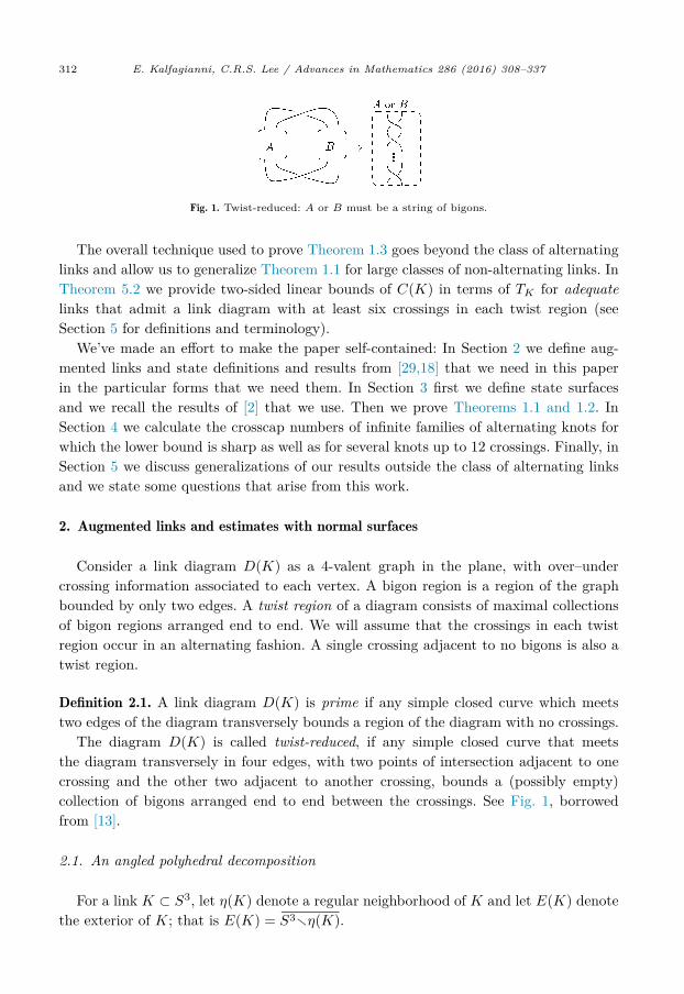
Fig. 1. Twist-reduced: A or B must be a string of bigons.

The overall technique used to prove Theorem 1.3 goes beyond the class of alternating links and allow us to generalize Theorem 1.1 for large classes of non-alternating links. In Theorem 5.2 we provide two-sided linear bounds of C(K) in terms of TK for adequatelinks that admit a link diagram with at least six crossings in each twist region (see Section 5 for definitions and terminology).

We’ve made an effort to make the paper self-contained: In Section 2 we define aug-mented links and state definitions and results from [29,18] that we need in this paper in the particular forms that we need them. In Section 3 first we define state surfaces and we recall the results of [2] that we use. Then we prove Theorems 1.1 and 1.2. In Section 4 we calculate the crosscap numbers of infinite families of alternating knots for which the lower bound is sharp as well as for several knots up to 12 crossings. Finally, in Section 5 we discuss generalizations of our results outside the class of alternating links and we state some questions that arise from this work.

2. Augmented links and estimates with normal surfaces

Consider a link diagram D(K) as a 4-valent graph in the plane, with over–under crossing information associated to each vertex. A bigon region is a region of the graph bounded by only two edges. A twist region of a diagram consists of maximal collections of bigon regions arranged end to end. We will assume that the crossings in each twist region occur in an alternating fashion. A single crossing adjacent to no bigons is also a twist region.

Definition 2.1. A link diagram D(K) is prime if any simple closed curve which meets two edges of the diagram transversely bounds a region of the diagram with no crossings.

The diagram D(K) is called twist-reduced, if any simple closed curve that meets the diagram transversely in four edges, with two points of intersection adjacent to one crossing and the other two adjacent to another crossing, bounds a (possibly empty) collection of bigons arranged end to end between the crossings. See Fig. 1, borrowed from [13].

2.1. An angled polyhedral decomposition

For a link K ⊂ S3, let η(K) denote a regular neighborhood of K and let E(K) denote the exterior of K; that is E(K) = S3�η(K).

E. Kalfagianni, C.R.S. Lee / Advances in Mathematics 286 (2016) 308–337 313

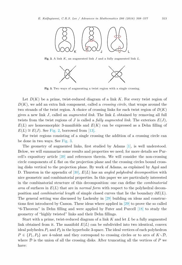
Fig. 2. A link K, an augmented link J and a fully augmented link L.

Fig. 3. Two ways of augmenting a twist region with a single crossing.

Let D(K) be a prime, twist-reduced diagram of a link K. For every twist region of D(K), we add an extra link component, called a crossing circle, that wraps around the two strands of the twist region. A choice of crossing links for each twist region of D(K)gives a new link J , called an augmented link. The link L obtained by removing all full twists from the twist regions of J is called a fully augmented link. The exteriors E(J), E(L) are homeomorphic 3-manifolds and E(K) can be expressed as a Dehn filling of E(L) ∼= E(J). See Fig. 2, borrowed from [13].

For twist regions consisting of a single crossing the addition of a crossing circle can be done in two ways. See Fig. 3.

The geometry of augmented links, first studied by Adams [1], is well understood. Below, we will summarize some results and properties we need; for more details see Pur-cell’s expository article [39] and references therein. We will consider the non-crossing circle components of L flat on the projection plane and the crossing circles bound cross-ing disks vertical to the projection plane. By work of Adams, as explained by Agol and D. Thurston in the appendix of [30], E(L) has an angled polyhedral decomposition with nice geometric and combinatorial properties. In this paper we are particularly interested in the combinatorial structure of this decomposition: one can define the combinatorial area of surfaces in E(L) that are in normal form with respect to the polyhedral decom-position and combinatorial length of simple closed curves that lie the boundary ∂E(L). The general setting was discussed by Lackenby in [29] building on ideas and construc-tions first introduced by Casson. These ideas where applied in [29] to prove the so called “6-Theorem” in Dehn filling and were applied by Futer and Purcell [18] to study the geometry of “highly twisted” links and their Dehn fillings.

Start with a prime, twist-reduced diagram of a link K and let L be a fully augmented link obtained from it. The manifold E(L) can be subdivided into two identical, convex ideal polyhedra P1 and P2 in the hyperbolic 3-space. The ideal vertices of each polyhedron P ∈ {P1, P2} are 4-valent and they correspond to crossing circles or to arcs of K�D, where D is the union of all the crossing disks. After truncating all the vertices of P we have:

314 E. Kalfagianni, C.R.S. Lee / Advances in Mathematics 286 (2016) 308–337

• Dihedral angles at each edge of P are π/2.• There are two types of edges of ∂P : these that are created by truncation called

boundary edges (edges of P ∩ ∂E(L)) and the ones that come from edges existing before truncation, called interior edges. The interior edges come from intersections of the crossing discs with the projection plane.

• There are two types of faces on ∂P : these that are created by truncation called boundary faces (faces of P ∩ ∂E(L)), and the ones that come from faces existing before truncation, called interior faces.

• Each boundary face is a rectangle that meets four interior edges at the vertices of the rectangle. The boundary faces of P1, P2 subdivide ∂E(J) into rectangles.

• The interior faces of P can be colored with two colors (shaded and white) in a checkerboard fashion so that at each rectangular boundary face of P opposite side interior faces have the same color. The shaded faces correspond to crossing disks while the white faces correspond to regions of the projection plane. See [30, Figure 15] and Fig. 12.

• The properties of the decomposition can in particular be used to prove that E(L) is hyperbolic.

The complement of all faces (interior and boundary) on the projection plane is a graph Γ ⊂ ∂P with vertices of valence at least three and edges the edges of P .

A polyhedral P with the above properties is called a rectangular-cusped polyhedron.

2.2. Normal surfaces and combinatorial area

In this paper we are interested in surfaces with boundary that are properly embedded in E(L) and are in normal form with respect to the above polyhedral decomposition. We recall the following definition.

Definition 2.2. A properly embedded surface (F, ∂F ) ⊂ (E(L), ∂E(L)) is said to be in normal form with respect to the polyhedra decomposition, if for any P ∈ {P1, P2} we have the following:

(1) F ∩ P consists of properly embedded disks (D, ∂D) ⊂ (P, ∂P ).(2) F ∩ ∂P is a collection of simple closed curves none of which lies entirely in a single

face of P .(3) F intersects faces of P in a collection of properly embedded arcs none of which passes

through vertices of Γ. Furthermore, none of these arcs runs from an edge of F to itself or from an interior edge to an adjacent boundary edge.

(4) A component of F ∩ P can intersect each boundary face in at most one arc.

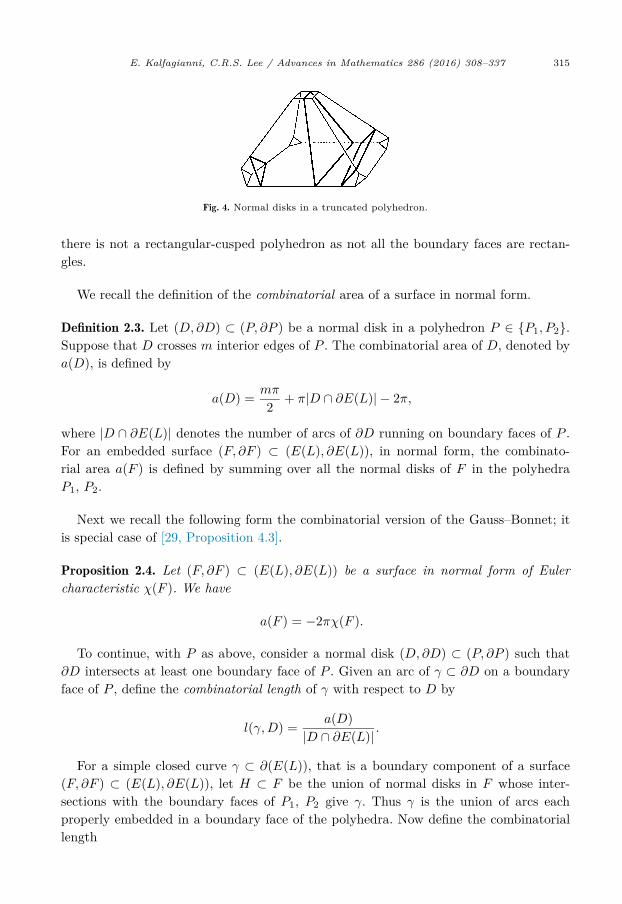
The components of F ∩ P are called normal disks. An example of three normal disks in a truncated polyhedron is shown in Fig. 4, borrowed from [18]. Note that P shown

E. Kalfagianni, C.R.S. Lee / Advances in Mathematics 286 (2016) 308–337 315

Fig. 4. Normal disks in a truncated polyhedron.

there is not a rectangular-cusped polyhedron as not all the boundary faces are rectan-gles.

We recall the definition of the combinatorial area of a surface in normal form.

Definition 2.3. Let (D, ∂D) ⊂ (P, ∂P ) be a normal disk in a polyhedron P ∈ {P1, P2}. Suppose that D crosses m interior edges of P . The combinatorial area of D, denoted by a(D), is defined by

a(D) = mπ

2 + π|D ∩ ∂E(L)| − 2π,

where |D ∩ ∂E(L)| denotes the number of arcs of ∂D running on boundary faces of P . For an embedded surface (F, ∂F ) ⊂ (E(L), ∂E(L)), in normal form, the combinato-rial area a(F ) is defined by summing over all the normal disks of F in the polyhedra P1, P2.

Next we recall the following form the combinatorial version of the Gauss–Bonnet; it is special case of [29, Proposition 4.3].

Proposition 2.4. Let (F, ∂F ) ⊂ (E(L), ∂E(L)) be a surface in normal form of Euler characteristic χ(F ). We have

a(F ) = −2πχ(F ).

To continue, with P as above, consider a normal disk (D, ∂D) ⊂ (P, ∂P ) such that ∂D intersects at least one boundary face of P . Given an arc of γ ⊂ ∂D on a boundary face of P , define the combinatorial length of γ with respect to D by

l(γ,D) = a(D)|D ∩ ∂E(L)| .

For a simple closed curve γ ⊂ ∂(E(L)), that is a boundary component of a surface (F, ∂F ) ⊂ (E(L), ∂E(L)), let H ⊂ F be the union of normal disks in F whose inter-sections with the boundary faces of P1, P2 give γ. Thus γ is the union of arcs each properly embedded in a boundary face of the polyhedra. Now define the combinatorial length

316 E. Kalfagianni, C.R.S. Lee / Advances in Mathematics 286 (2016) 308–337

lc(γ) := l(γ,H) =∑i

l(γi, D),

where the sum is taken over all normal disks in H and all normal arcs on boundary faces.

The quantity lc(γ), defined above, depends on F . To obtain a well defined notion of combinatorial length one needs to consider the infimum over all normal surfaces F and collections H with ∂F = γ. In fact, one can define the combinatorial length of any simple closed curve on ∂E(L) [29,18]. This is the definition of lc used by the authors in [18]. We will not repeat these definitions here as we don’t need them. However, the combinatorial length estimates of simple closed curves obtained in [18] also hold for l(γ, H). We need the following lemma that follows immediately from the above definitions.

Lemma 2.5. (See [18, Lemme 4.13].) Let (F, ∂F ) ⊂ (E(L), ∂E(L)) be an embedded sur-face in normal form with respect to the polyhedral decomposition and let γ1, . . . , γk denote the components of ∂F . Then,

a(F ) ≥k∑

j=1c(γj).

Finally we need the following.

Lemma 2.6. Suppose that E(L) is an augmented link obtained from a prime, twist-reduced link diagram D(K). Let (F, ∂F ) ⊂ (E(L), ∂E(L)) be an embedded normal surface and let γ be a component of ∂F that is homologically non-trivial on a component T ⊂ ∂E(L). If T comes from a crossing circle of L, let m denote the number of crossings in the corresponding twist region of D(K). If T comes from a component Kj of K, let m be the number of twist regions visited by Kj, counted with multiplicity. We have

c(γ) ≥ mπ

3 .

Proof. It is proven in the proof of [18, Corollary 5.12] using [18, Proposition 5.3]. �2.3. Genus estimates for spanning surfaces

Let (S, ∂S) ⊂ (E(K), ∂E(K)) be a spanning surface of K. That is a surface where the components of ∂S are the components of K and it contains no closed components. In fact, often, we will use (some times implicitly) the following convenient characterization of spanning surfaces.

Lemma 2.7. A properly embedded surface (S, ∂S) ⊂ (E(K), ∂E(K)), without closed com-ponents, is a spanning surface of K iff for each component of ∂E(K), the total geometric intersection number of the boundary curves ∂S with the corresponding meridian is 1.

E. Kalfagianni, C.R.S. Lee / Advances in Mathematics 286 (2016) 308–337 317

Proof. If S is a spanning surface of K, then clearly the desired conclusion holds. Con-versely, suppose that each component of ∂S has geometric intersection number 1 with the meridian on the component of ∂E(L) it lies. Then ∂S must have exactly one component on the corresponding component of ∂E(K). For, if we had more that one curves on some component of ∂E(K) then these curves will be parallel creating more intersections of ∂S with the corresponding meridian that would contribute to the geometric intersection number. Thus each component of ∂S is a longitude of ∂E(L). �

Let J be an augmented link obtained from a diagram of a K and let L be the cor-responding fully augmented link. A spanning surface (S, ∂S) ⊂ (E(K), ∂E(K)) gives a punctured surface (F, ∂F ) ⊂ (E(J), ∂E(J)). Now F gives a properly embedded surface (F ′, ∂F ′) ⊂ (E(L), ∂E(L)). Since we are only interested in the Euler characteristic of the surface we will often choose to work with F ′ instead of F . In fact, abusing the setting, we will identify F with F ′ and say we can view F as a surface in the exterior of the fully augmented link E(L) ∼= E(J). For the next theorem we will also assume that the surface F can be isotopied into normal form with respect to the polyhedral decomposition of E(L).

Theorem 2.8. Let K ⊂ S3 be a link of k components with a prime, twist-reduced diagram D(K). Suppose that D(K) has t ≥ 2 twist regions and let τ denote the smallest number of crossings corresponding to a twist region of D(K). Let S be a spanning surface of K and let L be an augmented link, obtained from K, such that S intersects n crossing circles of L. Suppose that the corresponding punctured surface F ⊂ E(L) can be isotopied to be normal with respect to the polyhedral decomposition P1, P2. Then we have

−χ(S) ≥⌈t

3 + nτ

6 − n

⌉.

Proof. The boundary ∂F consists of curves γ1, . . . , γk, one for each torus component of ∂E(L) that comes from a component of K and curves γk+1, . . . , γk+n on the compo-nents coming from crossing circles. By assumption F can be isotopied into normal form in the polyhedra P1 and P2; so we can compute its combinatorial area. By applying Proposition 2.4 and Lemma 2.5 we have

−2π · χ(S) = −2π · χ(F ) − 2πn = a(F ) − 2πn

≥k∑

i=1(γi) +

n∑i=1

(γk+i) − 2πn.

By Lemma 2.6, the total length of the curves γ1, . . . , γk is at least 2tπ/3, because Kpasses through each twist region twice. By the same lemma the total length of the curves γk+1, . . . , γk+n is at least nτπ/3. Thus from the last equation we obtain

318 E. Kalfagianni, C.R.S. Lee / Advances in Mathematics 286 (2016) 308–337

−2π · χ(S) ≥ 2tπ3 + nτπ

3 − 2πn

= 2π(t

3 + nτ

6 − n

).

Since the Euler characteristic is an integer, the conclusion follows. �Recall that for a non-orientable surface S, with k boundary components, the crosscap

number is defined to be C(S) = 2 − χ(S) − k. We have the following result that should be compared with [18, Theorem 1.5].

Corollary 2.9. Let the notation and setting be as in Theorem 2.8. Suppose moreover that D(K) has at least six crossings in each twist region and that S is non-orientable. Then we have

C(S) ≥⌈t

3

⌉+ 2 − k.

Proof. Let τ denote the smallest number of crossings corresponding to a twist region of D(K). By assumption, τ ≥ 6. Thus Theorem 2.8 gives

C(S) = −χ(S) + 2 − k ≥⌈t

3 + nτ

6 − n

⌉+ 2 − k

≥⌈t

3 + n− n

⌉+ 2 − k =

⌈t

3

⌉+ 2 − k. �

3. Alternating links

Adams and Kindred [2] gave an algorithm, starting with an alternating link projection, to construct spanning surfaces of maximal Euler characteristic among all the spanning surfaces of the link. Our goal in this section is to show that we can take such a spanning surface to lie in the complement of an appropriate augmented link obtained from the link projection. In the next section we will use the techniques of Section 2 to estimate the crosscap number of a prime alternating link in terms of the twist number and the crossing number of any prime, twist-reduced alternating diagram of the link.

3.1. State surfaces and a minimum overall genus algorithm

Given a crossing on a link diagram D(K) there are two ways to resolve it. A Kauffman state σ on D(K) is a choice of one of these two resolutions at each crossing of D(K). Given a state σ of D(K) we obtain a spanning surface Sσ of K, as follows: The result of applying σ to D(K) is a collection vσ(D) of non-intersecting circles in the plane, called state circles. We record the crossing resolutions along σ by embedded segments connecting the state circles. Each circle of vσ(D) bounds a disk in S3. These disks may

E. Kalfagianni, C.R.S. Lee / Advances in Mathematics 286 (2016) 308–337 319

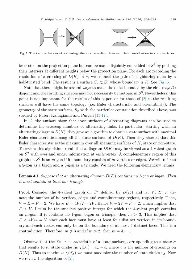
Fig. 5. The two resolutions of a crossing, the arcs recording them and their contribution to state surfaces.

be nested on the projection plane but can be made disjointly embedded in S3 by pushing their interiors at different heights below the projection plane. For each arc recording the resolution of a crossing of D(K) in σ, we connect the pair of neighboring disks by a half-twisted band. The result is a surface Sσ ⊂ S3 whose boundary is K. See Fig. 5.

Note that there might be several ways to make the disks bounded by the circles vσ(D)disjoint and the resulting surfaces may not necessarily be isotopic in S3. Nevertheless, this point is not important for the results of this paper, or for those of [2] as the resulting surfaces will have the same topology (i.e. Euler characteristic and orientability). The geometry of the state surfaces, Sσ with the particular construction described above, was studied by Futer, Kalfagianni and Purcell [15,17].

In [2] the authors show that state surfaces of alternating diagrams can be used to determine the crosscap numbers of alternating links. In particular, starting with an alternating diagram D(K), they gave an algorithm to obtain a state surface with maximal Euler characteristic among all the state surfaces of D(K). Then they showed that this Euler characteristic is the maximum over all spanning surfaces of K, state or non-state. To review this algorithm, recall that a diagram D(K) may be viewed as a 4-valent graph on S2 with over and under information at each vertex. A complementary region of this graph on S2 is an m-gon if its boundary consists of m vertices or edges. We will refer to a 2-gon as a bigon and a 3-gon as a triangle. We need the following elementary lemma.

Lemma 3.1. Suppose that an alternating diagram D(K) contains no 1-gon or bigon. Then it must contain at least one triangle.

Proof. Consider the 4-valent graph on S2 defined by D(K) and let V , E, F de-note the number of its vertices, edges and complimentary regions, respectively. Then, V − E + F = 2. We have E = 4V/2 = 2V . Hence V − 2V + F = 2, which implies that F > V . Let m be the smallest positive integer for which the 4-valent graph contains an m-gon. If it contains no 1-gon, bigon or triangle, then m > 3. This implies that F < 4V/4 = V since each face must have at least four distinct vertices in its bound-ary and each vertex can only be on the boundary of at most 4 distinct faces. This is a contradiction. Therefore, m ≯ 3 and if m > 2, then m = 3. �

Observe that the Euler characteristic of a state surface, corresponding to a state σthat results to vσ state circles, is χ(Sσ) = vσ − c, where c is the number of crossings on D(K). Thus to maximize χ(Sσ) we must maximize the number of state circles vσ. Now we review the algorithm of [2]:

320 E. Kalfagianni, C.R.S. Lee / Advances in Mathematics 286 (2016) 308–337

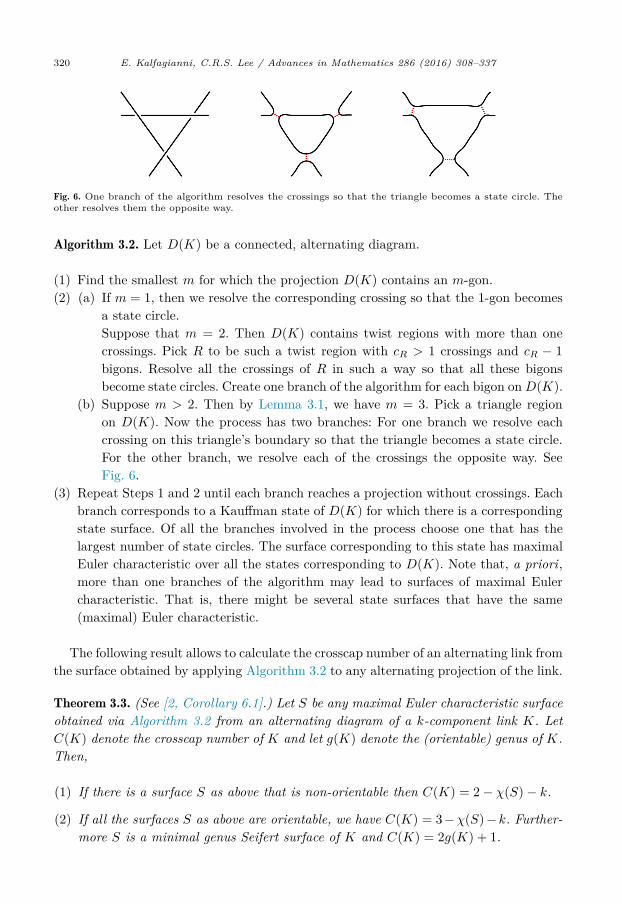
Fig. 6. One branch of the algorithm resolves the crossings so that the triangle becomes a state circle. The other resolves them the opposite way.

Algorithm 3.2. Let D(K) be a connected, alternating diagram.

(1) Find the smallest m for which the projection D(K) contains an m-gon.(2) (a) If m = 1, then we resolve the corresponding crossing so that the 1-gon becomes

a state circle.Suppose that m = 2. Then D(K) contains twist regions with more than one crossings. Pick R to be such a twist region with cR > 1 crossings and cR − 1bigons. Resolve all the crossings of R in such a way so that all these bigons become state circles. Create one branch of the algorithm for each bigon on D(K).

(b) Suppose m > 2. Then by Lemma 3.1, we have m = 3. Pick a triangle region on D(K). Now the process has two branches: For one branch we resolve each crossing on this triangle’s boundary so that the triangle becomes a state circle. For the other branch, we resolve each of the crossings the opposite way. See Fig. 6.

(3) Repeat Steps 1 and 2 until each branch reaches a projection without crossings. Each branch corresponds to a Kauffman state of D(K) for which there is a corresponding state surface. Of all the branches involved in the process choose one that has the largest number of state circles. The surface corresponding to this state has maximal Euler characteristic over all the states corresponding to D(K). Note that, a priori, more than one branches of the algorithm may lead to surfaces of maximal Euler characteristic. That is, there might be several state surfaces that have the same (maximal) Euler characteristic.

The following result allows to calculate the crosscap number of an alternating link from the surface obtained by applying Algorithm 3.2 to any alternating projection of the link.

Theorem 3.3. (See [2, Corollary 6.1].) Let S be any maximal Euler characteristic surface obtained via Algorithm 3.2 from an alternating diagram of a k-component link K. Let C(K) denote the crosscap number of K and let g(K) denote the (orientable) genus of K. Then,

(1) If there is a surface S as above that is non-orientable then C(K) = 2 − χ(S) − k.

(2) If all the surfaces S as above are orientable, we have C(K) = 3 −χ(S) −k. Further-more S is a minimal genus Seifert surface of K and C(K) = 2g(K) + 1.

E. Kalfagianni, C.R.S. Lee / Advances in Mathematics 286 (2016) 308–337 321

Fig. 7. A diagram of the knot 41 with bigon regions labeled 1 and 2 and the diagram resulting from applying the first step of Algorithm 3.2.

Fig. 8. Two algorithm branches corresponding to different bigons.

Example 3.4. We should clarify that different choices of branches as well as the order in resolving bigon regions following Algorithm 3.2 may result in different state surfaces. In particular at the end of the algorithm we may have both orientable and non-orientable surfaces that share the same Euler characteristic. We illustrate the subtlety in the algo-rithm by applying it to the knot 41.

Suppose that we choose the bigon labeled by 1 in the left hand side picture of Fig. 7. Then, for the next step of the algorithm, we have three choices of bigon regions to resolve, labeled by 1 and 2 and 3 in the right hand side picture of the figure.

The choice of bigon 1 leads to a non-orientable surface (left hand side picture of Fig. 8) while the choice of bigon 2 leads to an orientable surface (right hand side picture of Fig. 8). Both of these surfaces realize the maximal Euler characteristic of −1. The non-orientable surface realizes the crosscap number of 41, which is 2.

The next lemma is important for the results in this paper as it will allow us to apply the techniques of Section 2 to obtain bounds on crosscap numbers of alternating links.

Lemma 3.5. Let D(K) be a prime, alternating, twist-reduced knot diagram. There is a spanning surface S that is of maximal Euler characteristic for K, obtained by applying Algorithm 3.2 to D(K), and an augmented link J = JS such that S is in the complement E(J).

Proof. An augmented link is obtained from D(K) by adding a simple closed curve en-circling each twist region. If a twist region involves more than one crossing, then there is only one way to add a crossing circle. Otherwise, there are two ways of adding a crossing

322 E. Kalfagianni, C.R.S. Lee / Advances in Mathematics 286 (2016) 308–337

Fig. 9. The portion of S through a twist region with more than one crossing and the crossing circle for the twist region.

circle as shown in Fig. 3. Let S be a state surface with maximal Euler characteristic obtained by applying Algorithm 3.2 to D(K). We will show that there is such an S so that we can augment D(K) by making a choice of a crossing circle for each twist region involving a single crossing, such that S lies in the complement of the augmented link.

For a twist region R involving more than one crossing, and thus consists of a string of complementary bigon regions arranged end to end, we augment by adding a crossing circle CR encircling the twist region. Since D(K) is prime, none of its complementary regions can be an 1-gon. In this case, the algorithm picks the resolution of the crossings of R so that each bigon becomes a state circle following Step 2a. In any state surface which have this resolution at the crossings of R, these bigon disks are joined with twisted strips, and the crossing circle CR encloses the twisted strips. We may arrange so that each twisted strip intersects the crossing disk corresponding to CR only in its interior. Hence, the portion of any state surface obtained by the algorithm involving a twist region containing at least one bigon, will lie in the complement of CR. See Fig. 9.

Run Algorithm 3.2 till all the twist regions involving more than one bigon have been resolved and augmented as above. Let D′ be one of the resulting link diagrams at this stage of the algorithm. If there is a bigon on D′ that comes from a bigon in the original diagram D(K) then we apply step 1 of Algorithm 3.2 to this bigon and we add an augmentation component the same way as in Fig. 9.

Suppose that D′ contains a bigon that was not a bigon on D(K). Since D(K) is twist-reduced, such bigons in D′ can only come from triangles in D(K) that had a twist region with more than one crossings attached to them. If there is such a bigon in D′, Algorithm 3.2 will apply Step 2a to these crossings such that the bigon becomes a state circle. Then we choose an augmentation for each of the two crossings by putting two crossing circles, one for each of the two crossings resolved, so that each crossing circle encloses a twisting strip from the resolution at one crossing. The portion of the state surface coming from resolving these two crossings will then also be disjoint from the crossing circles. Repeat this procedure following the algorithm until there are no more bigons on the resulting diagrams D′.

Now each of the crossings on D′ corresponds to a twist region of D(K) containing a single crossing. We decide on which way to add a crossing circle to each of these twist regions. If there are no more crossings left in the projection, then we are done. Otherwise, we have a projection for whom a minimal n-gon is a triangle by Lemma 3.1, and Step 2b of the algorithm is applied to resolve each of the three crossings of the triangle, see Fig. 6.

E. Kalfagianni, C.R.S. Lee / Advances in Mathematics 286 (2016) 308–337 323

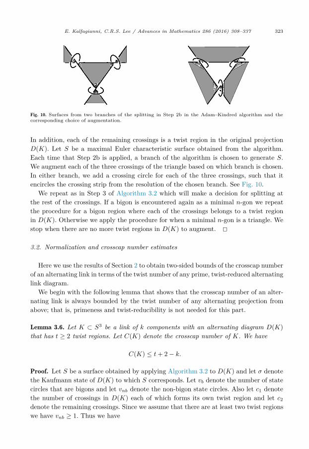
Fig. 10. Surfaces from two branches of the splitting in Step 2b in the Adam–Kindred algorithm and the corresponding choice of augmentation.

In addition, each of the remaining crossings is a twist region in the original projection D(K). Let S be a maximal Euler characteristic surface obtained from the algorithm. Each time that Step 2b is applied, a branch of the algorithm is chosen to generate S. We augment each of the three crossings of the triangle based on which branch is chosen. In either branch, we add a crossing circle for each of the three crossings, such that it encircles the crossing strip from the resolution of the chosen branch. See Fig. 10.

We repeat as in Step 3 of Algorithm 3.2 which will make a decision for splitting at the rest of the crossings. If a bigon is encountered again as a minimal n-gon we repeat the procedure for a bigon region where each of the crossings belongs to a twist region in D(K). Otherwise we apply the procedure for when a minimal n-gon is a triangle. We stop when there are no more twist regions in D(K) to augment. �3.2. Normalization and crosscap number estimates

Here we use the results of Section 2 to obtain two-sided bounds of the crosscap number of an alternating link in terms of the twist number of any prime, twist-reduced alternating link diagram.

We begin with the following lemma that shows that the crosscap number of an alter-nating link is always bounded by the twist number of any alternating projection from above; that is, primeness and twist-reducibility is not needed for this part.

Lemma 3.6. Let K ⊂ S3 be a link of k components with an alternating diagram D(K)that has t ≥ 2 twist regions. Let C(K) denote the crosscap number of K. We have

C(K) ≤ t + 2 − k.

Proof. Let S be a surface obtained by applying Algorithm 3.2 to D(K) and let σ denote the Kaufmann state of D(K) to which S corresponds. Let vb denote the number of state circles that are bigons and let vnb denote the non-bigon state circles. Also let c1 denote the number of crossings in D(K) each of which forms its own twist region and let c2denote the remaining crossings. Since we assume that there are at least two twist regions we have vnb ≥ 1. Thus we have

324 E. Kalfagianni, C.R.S. Lee / Advances in Mathematics 286 (2016) 308–337

−χ(S) = c2 − vb + c1 − vnb

≤ t− 1.

Now the upper bound follows at once from Theorem 3.3. �Before we are able to estimate C(K) from below we need some preparation. Let

D(K) be a link diagram and let J be an augmented link obtained from D(K) with L the corresponding fully augmented link. Suppose that the exterior E(J) ∼= E(L) is hyperbolic with an angled polyhedral decomposition {P1, P2} as described in Section 2. Let S be a spanning surface of K that realizes C(K). Having Lemma 3.5 in mind, we will also assume that S is disjoint from the crossing circles of J ; hence we can view it as a surface in E(J) ∼= E(L).

We wish to apply Theorem 2.8 to estimate χ(S). In order to do so we need to have Sin normal position with respect to the polyhedral decomposition {P1, P2}. The standard argument of making a surface that is incompressible and ∂-incompressible (that is, es-sential) normal in a triangulated 3-manifold [21], can be adjusted to work in the setting of more general polyhedral decompositions. The argument is written down by Futer and Guéritaud [12, Theorem 2.8]. Note however that surfaces that realize C(K) need not be essential in E(K). For instance, if all the state surfaces obtained from Algorithm 3.2applied to an alternating projection D(K) are orientable, then a spanning surface that realizes C(K) is obtained from a minimal genus Seifert surface by adding a half-twisted band. Such a surface is ∂-compressible. This, for example, happens for the knot 74 [2].

For our purposes we are only interested in the question of whether S can be converted to a spanning surface that is normal with respect to the polyhedral decomposition of E(L), without changing χ(S) and the surface orientability. For this we examine how a spanning surface S that realizes C(K) behaves under the general process that converts any properly embedded surface in E(J) into a normal one with possibly different topol-ogy [26]. We have the following lemma that applies beyond the class of alternating links and might be of independent interest.

Lemma 3.7. Let K ⊂ S3 be a link with a prime, twist-reduced diagram D(K). Suppose that D(K) has t ≥ 2 twist regions. Suppose that there is a spanning surface S in the exterior E(J) ∼= E(L) of an augmented link of D(K) and such that C(S) = C(K). Then exactly one of the following is true:

(1) There is a non-orientable, spanning surface S′ ⊂ E(L) for K, that is in normal form and such that χ(S) = χ(S′).

(2) We have C(K) = 2g(K) + 1. Furthermore, there is a Seifert surface of K that lies in E(L) such that it realizes g(K) and it is in normal form.

Proof. By assumption S realizes C(K). Thus S has maximal Euler characteristic among all non-orientable spanning surfaces of K. As discussed above, we will assume that S is

E. Kalfagianni, C.R.S. Lee / Advances in Mathematics 286 (2016) 308–337 325

not necessarily essential and examine how compressions and ∂-compressions may inter-fere with a process of converting S to a normal surface. Examining the moves required during this process [12, Theorem 2.8], and since S contains no closed components, we see that there are two situations to consider:

(1) S admits a compression disk D, that lies in the interior of a single face of a polyhedron P ∈ {P1, P2}.

(2) The intersection of S with a face of a polyhedron f ⊂ ∂P is an arc γ that runs from an edge of e ⊂ Γ ⊂ ∂P to itself, or from an interior edge to an adjacent boundary edge.

In (1) there are two cases to consider according to whether ∂D separates S or not. First suppose that ∂D is non-separating on S. Compressing along D we obtain a span-ning surface S′ for K with χ(S′) = χ(S) + 2. Since S realizes C(K), S′ cannot be non-orientable. Thus we have an orientable spanning surface of K; that is a Seifert sur-face. Adding a half-twisted band to S′ (i.e. adding a crosscap) produces a non-orientable spanning surface S1 of K with χ(S1) = χ(S′) − 1. Thus, S1 is a non-orientable spanning surface with χ(S1) = χ(S) + 1 > χ(S) which contradicts the fact that S realizes C(K). Thus this case will not happen.

Suppose now that ∂D separates S. We will look at such a disk so that ∂D is innermost in the sense that one of the components of S�∂D lies entirely in a single polyhedron P . Compressing along D gives two surfaces S1 and S2 with χ(S) = χ(S1) + χ(S2) − 2.

Suppose that both surfaces have non-empty boundary. Then the disjoint union of S1, S2 is a non-orientable spanning surface of K with Euler characteristic χ(S1) +χ(S2) >χ(S), contradicting the assumption that S realizes C(K). Thus, one of S1, S2, say S1, must be a closed surface and all of ∂S is left on S2. Since S1 is a closed surface embedded in S3, it is orientable. Hence S2 is a non-orientable. Since S realizes C(K) and χ(S1) ≤ 2, it follows that χ(S) = χ(S2). Thus we may ignore S2, replace S with S2 and continue with the normalization process.

Next we treat case (2): The arc γ cuts off a disk D ⊂ f , with ∂D consisting of γ and an arc that lies on the boundary of f . By an innermost argument, we may assume that the interior of D is disjoint from S. Again, following the argument in the proof of [12, Theorem 2.8], if γ runs from an interior edge to an adjacent boundary edge, the disk D will guide an isotopy of S that can be used to eliminate the arc γ [12, Figure 2.2]. Similarly, if e is an interior edge or e is a boundary edge and f is a boundary face, we can use D to obtain an isotopy that will eliminate γ and decrease the number of intersections of S with Γ (compare, left panel of [12, Figure 2.1]). It follows, that the only case left to examine is when e is a boundary edge and f is an interior face of S. In this case Dis a ∂-compression disk of S. Consider the arc δ := ∂D�γ ⊂ e and let T denote the boundary component of ∂E(K) containing it. There are two cases to consider: (i) δ cuts off a disk in the annulus T�∂S; and (ii) δ runs from one component of T�∂S. We will perform surgery (∂-compression) along D. This may cut S into more components

326 E. Kalfagianni, C.R.S. Lee / Advances in Mathematics 286 (2016) 308–337

or not according to whether we are in case (i) or (ii). Surgery along D doesn’t change the total geometric intersection number of ∂S with the meridians of ∂E(J). Thus, by Lemma 2.7, it will produce a spanning surface of K and possibly some (redundant) components.

First suppose that surgery along D splits S into two surfaces S1 and S2. Suppose that both surfaces have non-empty boundary. Then the disjoint union of S1, S2 is a non-orientable spanning surface of K with Euler characteristic χ(S1) + χ(S2) > χ(S), contradicting the assumption that S realizes C(K). Thus all the components of ∂Sdisjoint from D must remain on one of S1, S2, say on S2 and the intersections of ∂Swith the meridians of ∂E(K), also remain on ∂S2.

Thus S1 has one boundary component that is either homotopically trivial on ∂E(K)or isotopic to a meridian of ∂E(K). In either case ∂S1 bounds a disk in S3. We may cap ∂S1 with this disk to produce a closed surface embedded in S3, which must be orientable. Hence S2 is a non-orientable spanning surface for K. But since S realizes C(K) and χ(S1) ≤ 1 we must have χ(S) = χ(S2). Thus we may ignore S1, replace Swith S2 and continue with the normalization process.

Next suppose that surgery along D doesn’t disconnect S. Then we get a spanning surface S′, with χ(S′) = χ(S) + 1. Since S was assumed to realize C(K), S′ cannot be non-orientable. Thus we have an orientable spanning surface of K. We claim that S′

must be a minimal genus Seifert surface, that is g(S′) = g(K). For, suppose that K has a Seifert surface S1 with χ(S1) > χ(S′). Then adding a half-twisted band to S1 would give a non-orientable spanning surface S′′ with χ(S′′) = χ(S1) − 1 > χ(S′) − 1 = χ(S), contradicting the fact that S realizes C(K). Thus, S′ is a minimal genus Seifert sur-face of K that lies in E(L); that is we have g(S′) = g(K). Now it is clear that the surface obtained by a half-twisted band to S′ is a non-orientable spanning sur-face S′′ of K that has maximal Euler characteristic among all such surfaces. Thus we have C(K) = C(S′′) = 2g(S′) + 1 = 2g(K) + 1. Since S′ is minimal genus and ori-entable, it is incompressible and ∂-incompressible in E(K) and thus in E(L). Hence we may isotope S′ to be normal with respect to the polyhedral decomposition [12, Theo-rem 2.8]. �

Now we are ready to prove the following.

Theorem 3.8. Let K ⊂ S3 be a link of k components with a prime, twist-reduced alter-nating diagram D(K). Suppose that D(K) has t ≥ 2 twist regions. Let C(K) denote the crosscap number of K. We have

⌈t

3

⌉+ 2 − k ≤ C(K) ≤ t + 2 − k,

where �·� is the ceiling function that rounds up to the nearest larger integer. Furthermore, both bounds are sharp.

E. Kalfagianni, C.R.S. Lee / Advances in Mathematics 286 (2016) 308–337 327

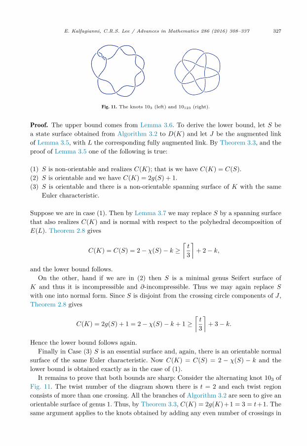
Fig. 11. The knots 103 (left) and 10123 (right).

Proof. The upper bound comes from Lemma 3.6. To derive the lower bound, let S be a state surface obtained from Algorithm 3.2 to D(K) and let J be the augmented link of Lemma 3.5, with L the corresponding fully augmented link. By Theorem 3.3, and the proof of Lemma 3.5 one of the following is true:

(1) S is non-orientable and realizes C(K); that is we have C(K) = C(S).(2) S is orientable and we have C(K) = 2g(S) + 1.(3) S is orientable and there is a non-orientable spanning surface of K with the same

Euler characteristic.

Suppose we are in case (1). Then by Lemma 3.7 we may replace S by a spanning surface that also realizes C(K) and is normal with respect to the polyhedral decomposition of E(L). Theorem 2.8 gives

C(K) = C(S) = 2 − χ(S) − k ≥⌈t

3

⌉+ 2 − k,

and the lower bound follows.On the other, hand if we are in (2) then S is a minimal genus Seifert surface of

K and thus it is incompressible and ∂-incompressible. Thus we may again replace Swith one into normal form. Since S is disjoint from the crossing circle components of J , Theorem 2.8 gives

C(K) = 2g(S) + 1 = 2 − χ(S) − k + 1 ≥⌈t

3

⌉+ 3 − k.

Hence the lower bound follows again.Finally in Case (3) S is an essential surface and, again, there is an orientable normal

surface of the same Euler characteristic. Now C(K) = C(S) = 2 − χ(S) − k and the lower bound is obtained exactly as in the case of (1).

It remains to prove that both bounds are sharp: Consider the alternating knot 103 of Fig. 11. The twist number of the diagram shown there is t = 2 and each twist region consists of more than one crossing. All the branches of Algorithm 3.2 are seen to give an orientable surface of genus 1. Thus, by Theorem 3.3, C(K) = 2g(K) +1 = 3 = t +1. The same argument applies to the knots obtained by adding any even number of crossings in

328 E. Kalfagianni, C.R.S. Lee / Advances in Mathematics 286 (2016) 308–337

each twist region of the knot 103. Hence we have an infinite family of alternating knots with C(K) = 2g(K) + 1 = 3 = t + 1.

To discuss some examples where our lower bound is sharp, note that if a knot Kprocesses an alternating diagram with c = t, then we have

1 +⌈ c3

⌉≤ C(K) ≤

⌊ c2

⌋.

Now observe that, for instance, if c = t = 13, then C(K) = 6. Similarly, if c = t = 10, then C(K) = 5. A concrete example, is the knot 10123 shown in Fig. 11. More examples where the lower bound is sharp are discussed in Section 4. �

Now we explain how Theorem 1.3, stated in the Introduction, follows from Theo-rem 3.8: For k = 1, the inequality of Theorem 3.8 becomes

⌈t

3

⌉+ 1 ≤ C(K) ≤ t + 1.

Thus the lower bound follows. Murakami and Yasuhara [35] showed that for a knot K with a connected, prime diagram of c crossings, we have

C(K) ≤⌊ c2

⌋.

Thus the upper bound follows from these two inequalities.

3.3. Jones polynomial bounds

Now we discuss how the results stated in the introduction follow from the above results. Recall that for a knot K, we have defined TK := |βK | + |β′

K |, where βK and β′K denote the second and the penultimate coefficients of the Jones polynomial of K,

respectively.

Theorem 1.1. Let K be a non-split, prime alternating link with k-components and with crosscap number C(K). Suppose that K is not a (2, p) torus link. We have

⌈TK

3

⌉+ 2 − k ≤ C(K) ≤ TK + 2 − k.

Furthermore, both bounds are sharp.

Proof. Let D(K) be a connected, twist-reduced alternating diagram that has t ≥ 2 twist regions. Then, by [11, Theorem 5.1], we have t = TK . A prime alternating link admits prime, twist-reduced alternating diagrams; every alternating diagram can be converted to a twist-reduced one by flype moves [30, Lemma 4]. Thus, the result follows from Theorem 3.8. �

E. Kalfagianni, C.R.S. Lee / Advances in Mathematics 286 (2016) 308–337 329

Now we are ready to prove Theorem 1.2 which we restate for the convenience of the reader.

Theorem 1.2. Let K be an alternating, non-torus knot with crosscap number C(K) and let TK be as above. We have

1 +⌈TK

3

⌉≤ C(K) ≤ min

{TK + 1,

⌊sK2

⌋}

where sK denotes the span of JK(t). Furthermore, both the upper and lower bounds are sharp.

Proof. Kauffman [27] showed that the degree span of the Jones polynomial of an alter-nating link is equal to the crossing number of the link. Furthermore, both the degree span and the crossing number of alternating knots are known to be additive under the operation of connect sum [31]. Using these, the upper inequality follows at once from Theorem 1.3. Furthermore, the lower inequality follows for all prime alternating knots.

To finish the proof we need to show that the lower inequality holds for connect sums of alternating knots. To that end let K#K ′ be such a knot. By [35], we have

C(K#K ′) ≥ C(K) + C(K ′) − 1.

Since the Jones polynomial is multiplicative under connect sum we have TK + TK′ ≥TK#K′ . Hence we have

C(K#K ′) ≥ C(K) + C(K ′) − 1 = TK

3 + TK′

3 + 4 − 2 − 1

≥ TK + TK′

3 + 1.

Hence the conclusion follows. �4. Calculations of crosscap numbers

4.1. Lower exact bounds

In this subsection we provide constructions and examples of families of alternatinglinks for which Theorem 3.8 gives the exact value of the crosscap number.

Let G be a trivalent planar graph and let N(G) denote a neighborhood of G on the plane. The boundary ∂N(G) is a link. For each edge of G we have two parallel arcs belonging on different components of ∂N(G). Construct a diagram of a new link by adding a number of half twists between these parallel arcs of the components ∂N(G)corresponding to each edge of G. Suppose that for each edge of G we add at least three crossings on D(K). We can do this so that the resulting diagram is alternating.

330 E. Kalfagianni, C.R.S. Lee / Advances in Mathematics 286 (2016) 308–337

Depending on the numbers of twists we put we may obtain a knot or a multi-component link. Let D(K) denote any alternating projection obtained this way and let SG be a state surface obtained from Algorithm 3.2 applied to D(K): Since each twist region contains bigons, SG corresponds to the Kauffman state of D(K) that resolves all the crossings so that the bigons are state circles. To analyze these surfaces further we need a definition.

Definition 4.1. A normal disk D in a polyhedron P ∈ {P1, P2} is called an ideal triangle if ∂D intersects exactly three boundary faces of ∂E(L) and it intersects no interior edges of P .

Corollary 4.2. Let K be a k-component link with a prime, twist-reduced alternating dia-gram D(K) constructed from a trivalent planar graph G as above. Then we have

C(K) =⌈t

3

⌉+ ε− k =

⌈TK

3

⌉+ ε− k,

where ε = 2 if SG is non-orientable and ε = 3 otherwise.

Proof. By assumption D(K) is obtained by adding twists along components of the boundary ∂N(G) of a regular neighborhood of a planar trivalent graph. The surface SG is obtained by N(G) by similar twisting and the augmented link of Lemma 3.5 is obtained by adding a component encircling each twist region of D(K). In order to calcu-late χ(SG) we need some more detailed information about the polyhedral decomposition {P1, P2} of E(L) [39]. The surface SG gives rise to surface S′

G in E(L); we will calculate χ(S′

G). Let D denote the union of the crossing disks bounded by the crossing circles of L. Each disk intersects the projection plane in a single arc. We may isotope the interior of S′

G so that it is disjoint from the intersections of D with the projection plane. Let P ∈ {P1, P2}. Recall that (before truncation) all the vertices of P are of valence four and they correspond to crossing circles of L and to arcs of K�D and the faces can be colored in a checkerboard fashion (in shaded and white) as follows:

(1) The shaded faces of P correspond to the crossing disks: Each disk D gives two triangular shaded faces of P meeting at an ideal vertex corresponding to the crossing circle ∂D (“bowties”).

(2) The edges of P come from the intersections of D with the projection plane.(3) The white faces of P correspond to regions of D(K) on the projection plane.

To a vertex v ∈ G there corresponds a triangular region of D(K) that is a neighbor-hood of v, around which the three twist regions D(K), corresponding to the edges of Gemanating from v, meet. Let Dv denote the union of the three crossing disks correspond-ing to the three twist regions of D(K) around v. This triangular region will become an ideal triangular white face, say Dv, after truncating the vertices of P . See Fig. 12. The ideal vertices of Dv come from the arcs of K�Dv that surround v. Each of the three

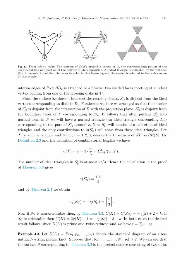
E. Kalfagianni, C.R.S. Lee / Advances in Mathematics 286 (2016) 308–337 331

Fig. 12. From left to right: The portion of D(K) around a vertex of G, the corresponding potion of the augmented link and portion of the polyhedral decomposition. An ideal triangle is indicated by the red line. (For interpretation of the references to color in this figure legend, the reader is referred to the web version of this article.)

interior edges of P on ∂Dv is attached to a bowtie: two shaded faces meeting at an ideal vertex coming from one of the crossing disks in Dv.

Since the surface SG doesn’t intersect the crossing circles, S′G is disjoint from the ideal

vertices corresponding to disks in Dv. Furthermore, since we arranged so that the interior of S′

G is disjoint from the intersection of D with the projection plane, S′G is disjoint from

the boundary faces of P corresponding to Dv. It follows that after putting S′G into

normal form in P we will have a normal triangle (an ideal triangle surrounding Dv) corresponding to the part of S′

G around v. Now S′G will consist of a collection of ideal

triangles and the only contributions to a(S′G) will come from these ideal triangles. Let

T be such a triangle and let γi, i = 1, 2, 3, denote the three arcs of ∂T on ∂E(L). By Definition 2.3 and the definition of combinatorial lengths we have

a(T ) = π = 3 · π3 = Σ3i=1l(γi, T ).

The number of ideal triangles in S′g is at most 2t/3. Hence the calculation in the proof

of Theorem 3.8 gives

a(S′G) = 2tπ

3 ,

and by Theorem 2.4 we obtain

−χ(SG) = −χ(S′G) =

⌈t

3

⌉.

Now if SG is non-orientable then, by Theorem 3.3, C(K) = C(SG) = −χ(S) + 2 − k. If SG is orientable then C(K) = 2g(K) + 1 = −χ(SG) + 3 − k. In both cases the desired result follows, since D(K) is prime and twist-reduced and we have t = TK . �Example 4.3. Let D(K) = P (p1, p2, . . . , pN ) denote the standard diagram of an alter-nating N -string pretzel knot. Suppose that, for i = 1, . . . , N , |pi| > 2. We can see that the surface S corresponding to Theorem 3.3 is the pretzel surface consisting of two disks

332 E. Kalfagianni, C.R.S. Lee / Advances in Mathematics 286 (2016) 308–337

Table 1Examples of knots where the Knotinfo upper bound agrees with our lower bound. The crosscap number is 3.

K TK K TK K TK K TK

1085 6 1093 6 10100 6 11a74 511a97 5 11a223 5 11a250 5 11a259 511a263 4 11a279 6 11a293 6 11a313 611a323 6 11a330 6 11a338 4 11a346 612a0636 5 12a0641 4 12a0753 5 12a0827 512a0845 5 12a0970 6 12a0984 6 12a1017 612a1031 5 12a1095 6 12a1107 6 12a1114 612a1142 5 12a1171 6 12a1179 6 12a1205 612a1220 6 12a1240 6 12a1243 4 12a1247 612a1285 4 – – – – – –

and N -twisted bands; one for each twist region of D(K). Augment the diagram D(K)by adding a crossing circle at each twist region so that the surface S intersects each crossing disk in a single arc only. This surface is disjoint from the crossing circles of the fully augmented link L. Furthermore, the surface S is essential in E(K) and thus in E(L). Hence we may put it in normal form to calculate the area a(S). By an argument similar to that in the proof of Corollary 4.2, it follows that the contributions to a(S)come from two identical, normal N -gons, D1, D2 such that ∂Di intersects N -boundary faces of the polyhedral decomposition and it intersects no interior edges. We have

a(S) = a(Di) + a(D2) = 2πN − 4π = 2π(TK − 2),

and thus −χ(S) = N − 2. If all, but one, pi are odd the S is non-orientable and thus C(K) = N − 1 = TK − 1. If all the pi’s are odd, then S is orientable and then, C(K) =N = TK . Note that the crosscap numbers of pretzel knots have been calculated in [25].

4.2. Low crossing knots

The crosscap numbers of all alternating links up to 9 crossings are known. Knotinfo [7]provides an upper and a lower bound for the crosscap numbers of all knots up to 12 crossings for which the exact values of crosscap numbers are not known. Note that in all, but a handful of cases, where the crosscap number is not determined, the lower bound given in Knotinfo is 2. There are 1778 prime, alternating knots with crossing numbers 10 ≤ c ≤ 12. For these knots we calculated the quantity TK := |βK | + |β′

K | using the Jones polynomial value given in Knotinfo and we compared our crosscap number lower bound with the one given in therein. For 1472 of these knots our lower bound is better than the one given in Knotinfo and for 283 of them our lower bound agrees with the upper bound in there; thus we are able to calculate the exact value of the crosscap number in these cases. These data have now been uploaded in Knotinfo by Cha and Livingston.

For example, in Table 1 we have all the 37 alternating knots K for which Knotinfo states 2 ≤ C(K) ≤ 3, together with the value of the corresponding quantity TK . In all

E. Kalfagianni, C.R.S. Lee / Advances in Mathematics 286 (2016) 308–337 333

the 37 cases the lower bound above is also 3; thus for all these knots we can determine the crosscap number to be 3.

5. Generalizations and questions

5.1. Non-alternating links

A question arising from this work is the question of the extent to which the Jones polynomial (coarsely) determines the crosscap number outside the class of alternating links. This is an interesting question that merits further investigation. Our contribu-tion towards an answer to this question, in this paper, is to provide a generalization of Theorem 1.1 for some class of non-alternating links. To state our result we need a definition.

Definition 5.1. For a link diagram D(K) let SA denote the state surface corresponding to the Kauffman state where all the crossings are resolved one way and let SB denote the state surface corresponding to the state where all crossings are resolved the opposite way.

A link K is called adequate if it admits a link diagram D(K) such that none of SA, SB

contains a half-twisted band with both ends attached on the same state circle.Adequate links form a large class that contains the alternating ones but it is much

wider. See [32,13,15].

Theorem 5.2. Let K be a k-component link with crosscap number C(K) and let TK be as above. Suppose that K admits a connected, twist-reduced, diagram D(K) that has t ≥ 2twist regions, and such that each twist region of D(K) contains at least six crossings. We have

⌈t

3

⌉+ 2 − k ≤ C(K) ≤ t + 2 − k.

If moreover D(K) is adequate then we have

⌈TK

6

⌉+ 2 − k ≤ C(K) ≤ 3TK − k − 1.

Proof. Let S be a spanning surface of K that is of maximal Euler characteristic over all spanning surfaces (that is both orientable and non-orientable). Then S gives an incom-pressible and ∂-incompressible surface in E(K). For, surgery of S along a compression or a ∂-compression disk will produce a surface of higher Euler characteristic (compare proof of Lemma 3.7). Let L be a fully augmented link obtained from D(K). Recall that each crossing circle added in this process bounds a disk D whose interior is pierced exactly twice by K. We will isotope S in the complement of K so that S∩D is minimized. In this

334 E. Kalfagianni, C.R.S. Lee / Advances in Mathematics 286 (2016) 308–337

process, since S is incompressible, if there is a simple closed curve in δ ⊂ S ∩ D that bounds a disk in D with its interior disjoint from S, then we can eliminate δ by isotopy of S in the complement of L. Similarly we can eliminate arc components of S ∩D that cut off disks on D with their interior disjoint from S. Finally, simple closed curves that are parallel to ∂D can be eliminated by sliding S off the boundary of D.

The surface S gives rise to a surface F in E(L). We claim that F is incompressible and ∂-incompressible in E(L). To see that, suppose that there is an essential simple closed curve γ ⊂ S that bounds a compressing disk in Δ ⊂ E(L). Since S is incompressible, γ must bound a disk Δ′ ⊂ S whose interior is intersected by the crossing circles of L. Now Δ ∪ Δ′ bounds a 3-ball that can be used to produce an isotopy that reduces the intersection of S and the crossing disks of L; contradiction.

Now we argue that F is ∂-incompressible. To that end, suppose that F admits a ∂-compression disk Δ, with ∂Δ = γ ∪ δ, where γ is a spanning arc in F and δ is an arc on a component T ⊂ ∂E(L). Assume, for a moment, that T corresponds to a component of K. Since S is ∂-incompressible in E(K), the arc γ must cut a disk Δ′ ⊂ S whose interior is pieced by the crossing circles of L. Since S is incompressible, the boundary of the disk Δ ∪Δ′ also bounds a disk Δ′′ ⊂ S. Now Δ′′ ∪Δ ∪Δ′ bounds a 3-ball that can be used to produce an isotopy that reduces the intersections of S with the crossing disks of L. This is a contradiction.

Suppose now that T is a component of ∂E(L) that corresponds to a crossing circle of L. Since S intersects crossing circles an even number of times, T�∂S has at least two components. Thus δ lies on an annulus A ⊂ T�∂S and either it cuts off a disk on A or it runs between different components of A. Now the usual argument that shows that an orientable, spanning surface of a link that is incompressible, has to be ∂-incompressible applies to obtain a contradiction (see [23, Lemma 1.10]). Thus the punctured surface Sis essential in E(L).

Now we may replace S by a surface, of the same orientability and Euler character-istic, that is in normal form with respect to the polyhedral decomposition of E(L) [12, Theorem 2.8]. Now Corollary 2.9 applies.

If S is non-orientable, we have C(S) = C(K) and by Corollary 2.9 we have

C(K) ≥⌈t

3

⌉+ 2 − k.

If S is orientable then C(K) = 2g(S) + 1 = 2g(K) + 1 and by Theorem 2.8 again we have C(K) ≥

⌈t3⌉

+ 2 − k. Combining these inequalities with Lemma 3.6 we have

⌈t

3

⌉+ 2 − k ≤ C(K) ≤ t + 2 − k,

which proves the first part of the theorem. Suppose now that D(K) is also adequate. Then [13, Theorem 1.5] implies that

E. Kalfagianni, C.R.S. Lee / Advances in Mathematics 286 (2016) 308–337 335

⌈t

3

⌉≤ TK ≤ 2t.

Now combining the last two inequalities gives the desired result. �Theorem 1.2 should be compared with Murasugi’s classical result [36] that the Alexan-

der polynomial determines the Seifert genus of alternating knots. The Alexander poly-nomial doesn’t determine the genus of non-alternating knots. However the Knot Floer Homology (the categorification of the Alexander polynomial) determines the genus of all knots [38]. A related question is the question of whether the Khovanov homology [28] of knots (the categorification of the Jones polynomial) is related to the crosscap number and the extent to which the former determines the later. We ask the following questions:

(1) For which links does the Jones polynomial (coarsely) determines C(K)?(2) Are there two sided bounds of C(K) of every link K in terms of the Khovanov

homology of K?

5.2. Combinatorial area and colored Jones polynomials

The colored Jones polynomial of a link K, is a sequence of Laurent polynomial in-variants.

JnK(t) = αnt

j(n) + βntj(n)−1 + . . . + β′

ntj′(n)+1 + α′

ntj′(n), n = 1, 2, . . .

with J2K(T ) being the ordinary Jones polynomial. It is known that, for every i > 0, the

absolute values of the i-th and the i-th to last coefficients of JnK(t) stabilize when i > n

[4,20]. For instance we have |β′K | := |β′

n|, and |βK | := |βn| for n > 1. The proofs of Theorem 1.1, Corollary 4.2, as well as Example 4.3, indicate that the quantity

TK

2π = |β′K | + |βK |

2π ,

is related to combinatorial areas of a normal surfaces in augmented links of K. One may ask whether the higher order stabilized coefficients of the colored Jones polynomials have similar interpretations. We will investigated this question in a future paper.

Acknowledgments

We thank Dave Futer and Jessica Purcell for several conversations and clarifications on the geometry of augmented links. Part of the results in this paper were obtained while Kalfagianni was visiting the Erwin Schrödinger International Institute for Mathematical Physics during the program “Combinatorics, Geometry and Physics” in the summer of 2014. She thanks the organizers of the program and the staff at ESI for providing excellent working conditions.

336 E. Kalfagianni, C.R.S. Lee / Advances in Mathematics 286 (2016) 308–337

References

[1] C.C. Adams, Augmented alternating link complements are hyperbolic, in: Low-Dimensional Topol-ogy and Kleinian Groups, Coventry/Durham, 1984, in: London Math. Soc. Lecture Note Ser., vol. 112, Cambridge Univ. Press, Cambridge, 1986, pp. 115–130.

[2] C. Adams, T. Kindred, A classification of spanning surfaces for alternating links, Algebr. Geom. Topol. 13 (5) (2013) 2967–3007.

[3] I. Agol, J. Hass, W. Thurston, The computational complexity of knot genus and spanning area, Trans. Amer. Math. Soc. 358 (9) (2006) 3821–3850.

[4] C. Armond, The head and tail conjecture for alternating knots, Algebr. Geom. Topol. 13 (5) (2013) 2809–2826.

[5] J. Batson, Nonorientable four-ball genus can be arbitrarily large, arXiv:1204.1985.[6] B.A. Burton, M. Ozlen, Computing the crosscap number of a knot using integer programming and

normal surfaces, ACM Trans. Math. Software 39 (1) (2012), Art. 4, 18.[7] J.C. Cha, C. Livingston, Knotinfo: table of knot invariants, http://www.indiana.edu/~knotinfo,

June 14 2014.[8] B.E. Clark, Crosscaps and knots, Int. J. Math. Math. Sci. 1 (1) (1978), 0161–1712.[9] R. Crowell, Genus of alternating link types, Ann. of Math. (2) 69 (1959) 258–275.

[10] O.T. Dasbach, D. Futer, E. Kalfagianni, X.-S. Lin, N.W. Stoltzfus, Alternating sum formulae for the determinant and other link invariants, J. Knot Theory Ramifications 19 (6) (2010) 765–782.

[11] O.T. Dasbach, X.-S. Lin, A volume-ish theorem for the Jones polynomial of alternating knots, Pacific J. Math. 231 (2) (2007) 279–291.

[12] D. Futer, F. Guéritaud, Angled decompositions of arborescent link complements, Proc. Lond. Math. Soc. (3) 98 (2) (2009) 325–364.

[13] D. Futer, E. Kalfagianni, J.S. Purcell, Dehn filling, volume, and the Jones polynomial, J. Differential Geom. 78 (3) (2008) 429–464.

[14] D. Futer, E. Kalfagianni, J.S. Purcell, Cusp areas of Farey manifolds and applications to knot theory, Int. Math. Res. Not. IMRN 2010 (23) (2010) 4434–4497.

[15] D. Futer, E. Kalfagianni, J.S. Purcell, Guts of Surfaces and the Colored Jones Polynomial, Lecture Notes in Mathematics, vol. 2069, Springer, Heidelberg, 2013.

[16] D. Futer, E. Kalfagianni, J.S. Purcell, Jones polynomials, volume, and essential knot surfaces: a sur-vey, in: Proceedings of Knots in Poland III, vol. 100, Banach Center Publications, 2014, pp. 51–77.

[17] D. Futer, E. Kalfagianni, J.S. Purcell, Quasifuchsian state surfaces, Trans. Amer. Math. Soc. 366 (8) (2014) 4323–4343.

[18] D. Futer, J.S. Purcell, Links with no exceptional surgeries, Comment. Math. Helv. 82 (3) (2007) 629–664.

[19] S. Garoufalidis, The Jones slopes of a knot, Quantum Topol. 2 (1) (2011) 43–69.[20] S. Garoufalidis, T.T.Q. Lê, Nahm sums, stability and the colored Jones polynomial, Res. Math. Sci.

2 (2015) 1–5.[21] W. Haken, Theorie der Normalflächen, Acta Math. 105 (1961) 245–375.[22] J. Hass, J.C. Lagarias, N. Pippenger, The computational complexity of knot and link problems,

J. ACM 46 (2) (1999) 185–211.[23] A. Hatcher, Notes on basic 3-manifold topology, http://www.math.cornell.edu/~hatcher/3M/

3Mdownloads.html.[24] M. Hirasawa, M. Teragaito, Crosscap numbers of 2-bridge knots, Topology 45 (3) (2006) 513–530.[25] K. Ichihara, S. Mizushima, Crosscap numbers of pretzel knots, Topology Appl. 157 (1) (2010)

193–201.[26] W. Jaco, J.H. Rubinstein, PL equivariant surgery and invariant decompositions of 3-manifolds, Adv.

Math. 73 (2) (1989) 149–191.[27] L.H. Kauffman, State models and the Jones polynomial, Topology 26 (3) (1987) 395–407.[28] M. Khovanov, A categorification of the Jones polynomial, Duke Math. J. 101 (3) (2000) 359–426.[29] M. Lackenby, Word hyperbolic dehn surgery, Invent. Math. 140 (2) (2000) 243–282.[30] M. Lackenby, The volume of hyperbolic alternating link complements, Proc. Lond. Math. Soc. (3)

88 (1) (2004) 204–224, with an appendix by Ian Agol and Dylan Thurston.[31] W.B.R. Lickorish, An Introduction to Knot Theory, Graduate Texts in Mathematics, vol. 175,

Springer-Verlag, New York, 1997.[32] W.B.R. Lickorish, M.B. Thistlethwaite, Some links with nontrivial polynomials and their crossing-

numbers, Comment. Math. Helv. 63 (4) (1988) 527–539.

E. Kalfagianni, C.R.S. Lee / Advances in Mathematics 286 (2016) 308–337 337

[33] W.W. Menasco, Closed incompressible surfaces in alternating knot and link complements, Topology 23 (1) (1984) 37–44.

[34] H. Murakami, An introduction to the volume conjecture, in: Interactions Between Hyperbolic Ge-ometry, Quantum Topology and Number Theory, in: Contemp. Math., vol. 541, Amer. Math. Soc., Providence, RI, 2011, pp. 1–40.

[35] H. Murakami, A. Yasuhara, Crosscap number of a knot, Pacific J. Math. 171 (1) (1995) 261–273.[36] K. Murasugi, On the Alexander polynomial of the alternating knot, Osaka J. Math. 10 (1958)

181–189; errata, Osaka J. Math. 11 (1959) 95.[37] K. Murasugi, Jones polynomials and classical conjectures in knot theory, Topology 26 (2) (1987)

187–194.[38] P. Ozsváth, Z. Szabó, Holomorphic disks and genus bounds, Geom. Topol. 8 (2004) 311–334.[39] J.S. Purcell, An introduction to fully augmented links, in: Interactions Between Hyperbolic Geom-

etry, Quantum Topology and Number Theory, in: Contemp. Math., vol. 541, Amer. Math. Soc., Providence, RI, 2011, pp. 205–220.

[40] M. Teragaito, Crosscap numbers of torus knots, Topology Appl. 138 (1–3) (2004) 219–238.