Retrospective Theses and Dissertations Iowa State University Capstones, Theses andDissertations

1964

Mass transfer studies in forming and collapsingdropletsJohn Orville GoldenIowa State University

Follow this and additional works at: https://lib.dr.iastate.edu/rtd

Part of the Chemical Engineering Commons

This Dissertation is brought to you for free and open access by the Iowa State University Capstones, Theses and Dissertations at Iowa State UniversityDigital Repository. It has been accepted for inclusion in Retrospective Theses and Dissertations by an authorized administrator of Iowa State UniversityDigital Repository. For more information, please contact digirep@iastate.edu.

Recommended CitationGolden, John Orville, "Mass transfer studies in forming and collapsing droplets " (1964). Retrospective Theses and Dissertations. 2988.https://lib.dr.iastate.edu/rtd/2988

This dissertation has been 64-9265 microfilmed exactly as received

GOLDEN, John Orville, 1937-MASS TRANSFER STUDIES IN FORMING AND COLLAPSING DROPLETS.

Iowa State University of Science and Technology Ph.D., 1964 Engineering, chemical

University Microfilms, Inc., Ann Arbor, Michigan

MASS TRANSFER STUDIES IN

FORMING AND COLLAPSING DROPLETS

by

John Orville Golden

A Dissertation Submitted to the

Graduate Faculty in Partial Fulfillment of

The Requirements for the Degree of

DOCTOR OF PHILOSOPHY

Major Subject: Chemical Engineering

Approved :

n Charge of Major Work

Head of Major Department

Iowa State University Of Science and Technology

Ames, Iowa

1964

Signature was redacted for privacy.

Signature was redacted for privacy.

Signature was redacted for privacy.

ii

TABLE OF CONTENTS

. Page

INTRODUCTION 1

PREVIOUS WORK 3

PRINCIPLES OF MASS TRANSFER IN DROPLET SYSTEMS 16

SYSTEM 24

EXPERIMENTAL APPARATUS 28

EXPERIMENTAL PROCEDURE 37

DESCRIPTION OF MASS TRANSFER MODELS 41

RESULTS 58

CONCLUSIONS AND RECOMMENDATIONS 87

NOMENCLATURE 90

LITERATURE CITED 92

ACKNOWLEDGEMENTS 95

APPENDIX A 96

APPENDIX B 106

APPENDIX C 120

APPENDIX D 122

1

INTRODUCTION

In the past, chemical engineers have had to rely

primarily on empirical methods in dealing with commercial

extraction equipment. During the past several years there

has been an increasing emphasis toward a more fundamental

understanding of the mass transfer mechanism in liquid-liquid

extraction. Consequently, research emphasis in solvent ex­

traction is changing from studies on small scale laboratory

columns to areas dealing with the chemistry of the liquid

state, interfacial and drop phenomena, and the mathematical

description of the solute transfer process. Although empirical

methods were sufficient in the past for commercial operations,

a more fundamental basis is necessary to fulfill the increasing

demands made by industry upon solvent extraction as a unit

operation.

Most liquid-liquid extraction equipment involves transfer

between two phases, one of which is dispersed as droplets

in the other. Past workers who studied transfer from liquid

drops have proposed three different stages in the life of a

drop--drop formation, drop rise or fall, and drop coalescence.

The actual mass transfer process is more complicated because

different mechanisms probably predominate in each of these

three stages.

In order to understand the transport process in all

three stages, it is necessary to understand the transport of

2

a solute across a liquid-liquid interface, which is a complex

phenomenon. However, the problem becomes increasingly more

difficult when the interfacial area is varying with time and

there is fluid motion in the region of the liquid-liquid

interface. A great deal of research has been devoted to mass

transport across liquid-liquid interfaces and droplet phenom­

ena, however, our understanding of the subject is still

rudimentary. Therefore, a study was undertaken of mass trans­

port across a moving liquid-liquid interface under idealized

conditions, with the goal in view of learning more about the

mechanism of extraction and testing a number of models for

the mass transport process.

Generation of the liquid-liquid interface was accomplished

by forming a large organic droplet on a stainless steel tube,

which was immersed in a water phase. A series of droplets

was formed and collapsed under a variety of conditions and the

amount of solute transfer measured. From this experimental

data, a study was made of the factors that affect the extrac­

tion process and three theoretical models for the transport

process were tested.

3

PREVIOUS WORK

Small Column Studies

The first study of mass transfer between single drops and

a continuous phase was carried out by Sherwood, Evans, and

Longcor (24). Although previous work had been done on spray

columns, they were the first to attempt to study extraction

from single drops. They were unable to separate experimentally

the extraction in the three stages of a droplet life. However,

they did attempt to estimate the extraction occurring during

drop formation. By plotting the ratio of the unextracted

solute to the total solute which could be extracted if equilib­

rium were attained against column height, they found that 40%

of the extraction occurred during the formation period. They

assumed that by extrapolating back to zero column height,

they were able to determine the extraction during the formation

period.

Since the work of Sherwood et al. (24), a number of

investigations (6, 20, 21, 30, 31) have attempted to deal with

the mass transfer process occurring in single drops. These

workers recognized the three different periods in the life of

a drop and could be classed together since they used a similar

experimental technique to approach the problem of mass transfer

during drop formation. None of the workers were able to

separate experimentally the transfer which took place during

drop formation, but rather relied upon extrapolation techniques

4

to examine the formation period. Experimental values for the

amount of extraction during the formation period ranged from

7 to 20%. Licht and Pansing (21) concluded from their work

that the extrapolation technique used by earlier workers

was inaccurate, since a plot of per cent extracted versus

column height yielded a curved rather than a straight line at

short column heights.

An investigation by Coulson and Skinner (2) is of special

importance since it was the first attempt made to study the

effect of the drop formation period itself. Using an apparatus

that formed drops on a capillary tip and subsequently col­

lapsed them, they were able to eliminate entirely the rise

and coalescence periods. For their system, they chose benzene

as the droplet phase and water as the continuous phase, while

they employed both benzoic and propionic acids as solutes.

However, there were several drawbacks to this technique for

determining the transfer during the formation period. First,

the nozzle of their apparatus was constructed so that there

was a small volume through which liquid passed in both forming

and collapsing a drop. When the drop was formed, this volume

was never exposed to the continuous phase and was rejected

from the nozzle along with the drop. The authors state that

a correction was made for this channeling effect. Second, it

took a period of time for the drop to collapse, so that the

actual exposure time of the drop was equal to the time of

formation plus the time of collapse. Therefore, the data

5

really represented the extraction taking place during the

formation and collapse of the drop.

From their study, Coulson and Skinner reached the

following conclusions :

(1) Mass transfer to a drop during the formation period

was found to be almost independent of the time of formation

of the droplet for a range of one half to one second for

formation.

(2) The overall mass transfer coefficient based on the ' '»

average area exposed during the formation of the drop decreases

with increasing time of formation, but is practically inde­

pendent of the drop size.

(3) Smaller drops approached equilibrium more closely

because of the increased interfacial area per unit volume.

The authors concluded that the mass transfer into a

droplet is independent of the time of formation. However,

their data do not agree with this conclusion as may be seen

in Figures 3 and 4 of reference (2). Coulson and Skinner

attempted to compare their results with those predicted by

simple unsteady state diffusion into a stagnant liquid. They

found their individual mass transfer coefficients varied

_ 0 "7 nearly as t^ ' (t^ is the time of formation) whereas simple

diffusion theory predicts a dependence on the time of forma­

tion of t£ ̂ ^ .

One of the more recent studies of mass transfer during

the formation period, was by Gregory (9). Gregory used what

6

he considered to be an improved version of Coulson and

Skinner's apparatus. Like Coulson and Skinner's apparatus,

a drop was formed on the end of a nozzle and subsequently

rejected through a separate channel. Gregory had a linear

rate of formation of the drop and eliminated the channeling

effect which Coulson and Skinner had in their apparatus.

Where Coulson and Skinner had approximately equal time of

formation and collapse, Gregory collapsed his drop almost

instantaneously. He said that with a small time of collapse,

the amount of extraction during the collapse period would tend

to be reduced or eliminated. It should be pointed out that

a rapid rate of collapse would tend to cause turbulence

within the drop having an undetermined effect on the amount

of solute transferred. Gregory used systems .where the equilib­

rium strongly favored the continuous phase so that the major

resistance to mass transfer would lie in the dispersed phase.

The majority of his data was taken using acetic acid dissolved

in carbon, tetrachloride as the dispersed phase and water as

the continuous phase.

He proposed five possible mechanisms to explain the mass

transfer process during drop formation:

1. Turbulence throughout the whole drop may be so great

that the bulk concentration of the dispersed phase is the

same as the interface concentration, and.there is no dispersed

phase resistance.

7

2. Mass transfer may take place by molecular or eddy

diffusion throughout the entire forming drop with the fresh

liquid entering at the center and pushing the older portions

of the liquid uniformly and without mixing toward the surface.

3. Mass transfer may take place by diffusion throughout

the entire forming drop with the entering liquid distributing

itself uniformly, so that none of the older liquid is displaced

from its position relative to the interface of the drop.

4. Circulation within the drop may cause constant

renewal of the elements of liquid next to the surface. Mass

transfer is by diffusion within these surface elements which

in turn mix with the bulk liquid .in the drop.

5. The film theory mechanism which postulates the

presence of a laminar film resistance next to the interface

and an inner turbulent film. The laminar film must be thin

enough so that any change in the quantity of solute present

in the film is negligible compared to the change undergone

by the bulk.

Gregory was plagued with many experimental difficulties.

Residual drop formation on the tip of the capillary during

the experimental runs was a problem that had to be carefully

checked. This occurred when a drop failed to be completely

rejected into the nozzle during the collapse period. Leaks

and air pockets in the apparatus also caused difficulty.

The primary criticism of his work would be that his experi­

mental error was of the order of magnitude of the changes in

8

mass transfer he was.trying to measure.

He found that no single mechanism correlated his data.

A satisfactory correlation was found with the film theory,

particularly with acetic acid in carbon tetrachloride dispersed

phase data, which covered the most extensive range of variables.

His best final correlation for all systems in which the drop

phase was lighter than the continuous was

in which d is drop diameter, D is the molecular diffusivity

in the dispersed phase, k, is the dispersed phase mass transfer

coefficient, and v is the jet velocity at the orifice of the

nozzle.

Gregory concluded that since the film theory (mechanism

5) predicted the amount of extraction properly for some

systems and a diffusion mechanism (mechanism 2) for other

systems, it was postulated that if,

where t^ is the time of formation, the film theory applied.

Otherwise, mass transfer was by diffusion throughout the

drop (mechanism 2).

He concludes from his overall results that at low nozzle

jet velocity and long formation times mass transfer is by

diffusion throughout the whole forming drop. As the jet

jjd = 3.74 (dvp ) ® ^ (jx_) ^ (1) v |i pD

( 2 )

9

velocity increases, mass transfer takes place through a flim

next to the surface that is primarily laminar with a turbulent

core. Further increase in the jet velocity results in turbu­

lence. extending to the surface and a third mechanism controls

the rate of mass transfer.

Another recent work in this area is presented by Johnson,

et al. (14). This paper is concerned with end effect correc­

tions in heat and mass transfer studies. The authors present

plotting methods to determine the "end effect"--mass transfer

during drop formation--for various models. The difficulty

here is that a model or mechanism must be known or assumed

before these end effects can be determined. Previous work

had shown that determining the mechanism is a problem in

it self.

Michels (22), in another recent work, has studied the

mechanism of mass transfer occurring during the formation of

a gas droplet in a liquid phase. He has presented equations

for a diffusion mechanism and suggests that these equations

may be applied to a liquid droplet. Also, he suggests that

motion of the interfacial boundary introduces a transport

term in the diffusion equation which strongly affects the

rate of diffusion.' The effect of the motion of the fluid

medium is to sharpen concentration gradients, and thereby,

to increase mass transfer rates.

In surveying the literature on mass transfer during

drop formation in liquid-liquid systems, two points should be

10

mentioned. First, the results of the various investigators

are often system dependent, so that it is difficult to compare

the results of the various workers and make significant

generalizations. Second, there are serious experimental

difficulties in trying to study mass transfer from very small

drops, as most previous investigators have attempted to do.

As evidenced by a review of the literature, our under­

standing of the mass transfer process during drop formation

is rudimentary. The discrepancies of past investigations

indicate a need for more work in this area.

Transfer Through Liquid-Liquid Interfaces

There have been a number of good review articles (11,

13, 27, 34) published recently which cover the areas of mass

transfer, liquid extraction, transfer to interfaces, and the

effect of surface active agents on liquid-liquid mass transfer.

In 1923, Whitman (32) proposed the film theory, which

has been used extensively for the correlation of extraction

data. Older versions of the theory imply a stagnant film at

the interface with the rate of transfer controlled by the rate

of molecular diffusion through a nearly stagnant film. Al­

though the film theory does not give an accurate picture of

the transfer process, the method of adding the resistances of

the two phases and the assumption of equilibrium at the inter­

face are essential parts of many current theories. Gregory

(9) in his treatment of transfer during drop formation in

11

liquid-liquid extraction used a modification of the film

theory as one possible model for the transfer process. He

postulated an inner turbulent core of the droplet, where

transfer was controlled by diffusion through a laminar film

on the surface.

Higbie (12) in dealing with gas absorption in a liquid,

was the first to apply what is presently termed the penetra­

tion theory. The penetration theory is simply the expression

for the rate of molecular diffusion into an infinite slab

with the boundary conditions of uniform concentration at

time zero, and a constant surface concentration for all times

greater than zero. Danckwerts (3) and Kishinevsky (16)

extended the penetration theory, reasoning that there would

be a distribution of contact times in most contacting devices,

rather than a constant contact time for all elements of the

interface. The penetration theory has been applied by

several investigators to single droplet extraction (2, 9) with

rather limited success. Combining the ideas of Higbie and

Danckwerts yields the well known surface renewal concept in

which the elements of volume in the region of the surface are

constantly being renewed by fluid motion. Transfer from these

volume elements may be by molecular or eddy diffusion,

depending upon the mechanism postulated.

A recent work by Harriott (10) proposed a random eddy

modification of the penetration theory. The author postulated

a model where transfer is accomplished by the motion of eddies

12

coupled with molecular diffusion when the eddies are not present.

Beek and Kramers (l), in attempting to deal with the mass

transfer process with a changing interfacial area, use the

penetration theory to develop what they term a "crude" theory

for the transfer process. They arrive at only an approximate

solution for the case of a growing droplet with spherical

geometry.

Kronig and Brink (17) made theoretical calculations on

the mass transfer process in circulating and stagnant drop­

lets in liquid-liquid extraction. They assumed that circula­

tion was produced by viscous forces during drop fall or rise

and that the problem was one of combining the hydrodynamics

of the problem with the diffusional processes. They found

that the time for 63% extraction from a stagnant drop was

2.5 times greater than for a circulating drop.

Michels (22) developed equations for the mechanism of

mass transfer during the formation period of a gas bubble

or liquid droplet. He modified the penetration theory to

include a transport term resulting from fluid motion near

the interfacial boundary. His results indicated that this

type of model would work for the transfer process in gas

absorption for a single bubble. However, he presented no

experimental evidence to confirm the utility of this model

for a liquid-liquid system.

Virtually all of the theoretical models for the transfer

process in a single droplet have assumed spherical geometry

13

of the droplet. This condition can be meant in many experi­

mental systems, particularly with very small droplets,

although, in many cases this condition is quite restrictive.

Interfacial Activity

Quite often during the transfer of a solute between two

liquid phases, spontaneous turbulence of the liquid-liquid

interface occurs. The interface may be mildly active with

rippling or pulsations, or there may be intensely turbulent

conditions with spontaneous emulsification occurring at the

interface of the two liquids. This phenomenon has been

observed by many investigators in a variety of systems (18,

19, 25, 29). Often, very high mass transfer rates are

reported when this phenomenon is observed in the system

under consideration.

Davies and Rideal (4), in 1961, presented an interesting

review of liquid-liquid interfacial turbulence in discussing

diffusion through liquid-liquid interfaces. Not only do

they discuss many of the past observations of interfacial

activity in liquid-liquid systems but they also present a

number of simple qualitative theories that have been proposed

to explain the cause of interfacial instability and the

resulting increased mass transfer.

Sherwood and Wei (25) noted interfacial turbulence in

40 different systems involving immiscible liquids. Activity

was noted in some systems in which a single solute was

14

extracted without chemical reaction, but the effects were

usually more pronounced in cases of exothermic neutralization

reactions. The interfacial activity was a strong function

of solute concentration, and was generally greater for trans­

fer from the organic to the aqueous phase than for transfer

in the opposite direction.

Sternling and Scriven (26) have developed a simplified

mathematical model for the mechanism of interfacial turbulence

using classical hydrodynamics, diffusional principles, and

surface chemistry. They suggest that the essence of the

explanation lies in the Marangoni effect, where movement in

the interface is caused by longitudinal variations of inter-

facial tension. They propose, "that interfacial turbulence is.

a manifestation of hydrodynamic instability,which is touched

off by ever present, small, random fluctuations about the

interface." The model in its simplified state yields only

criteria for the onset of instability, and cannot yet be

used to predict mass transfer rates.

One of the most detailed investigations of interfacial

turbulence in a given system has been made by Orell and

Westwater (23) in a photographic study on the ethylene

glycol-acetic acid-ethyl acetate system. They found that the

interface exhibited a dominant pattern of stationary and

propagating polygonal cells, accompanied by stripes, cell

15

cluster boundariesj and confined or unconfined ripples. In

an attempt to test the Sternling-Scriven theory, they con­

cluded what Sternling and Scriven had stated earlier--the

theory is too simplified to be reproduced experimentally.

16

PRINCIPLES OF MASS TRANSFER IN DROPLET SYSTEMS

In considering maSs transfer between two liquid phases,

with one phase dispersed as droplets in the other, a basic

equation can be given,

iT^" - 17^ + (Rj) + JL (3) Ky "d i kc

where:

Ky = overall mass transfer coefficient,

k-, = mass transfer coefficient basdd on the droplet phas

k = mass transfer coefficient based on the continuous phase,

m = distribution coefficient defined by m = C ,

where C, and C are concentrations of solute in the

droplet and continuous phases which are in equilibrium.

According to Equation (3), the resistance to mass transfer in

a drop is equal to the sum of three resistances, the resistanc

encountered in the drop itself, the interfacial resistance,

and the resistance due to the continuous phase. Assuming

negligible interfacial resistance, k, and k of approximately

equal magnitude, and a very small distribution coefficient,

the majority of the resistance will be found in the droplet

itself. A low distribution coefficient would result from

the solute strongly favoring the continuous phase. Choosing

a system in which the solute has a much lower diffusivity in

the droplet phase than in the continuous phase, would also

help place the primary resistance in the droplet phase.

17

Therefore, by appropriately choosing the system, a study of

the mass transfer process in the droplet may be based on the

drop phase controlling the rate of transfer.

A number of models for the mass transfer process in the

droplet phase have been proposed by previous investigators.

Five general types may be given:

(1) Models based on a molecular diffusion mechanism;

(2) Models based on a diffusional mechanism coupled

with internal fluid motion;

(3) Models based on an eddy diffusional process ;

(4) Models based in a surface renewal mechanism

(penetration theory);

(5) Models based on a film theory mechanism.

The mathematics of the above models have received a great

deal of attention for droplets where the assumption of

constant spherical geometry is made. However, when the volume

and interfacial area of the droplet are functions of time,

the rigorous mathematical treatment of the above models

becomes very complex and approximate procedures are necessary.

Here several points should be mentioned. First, it is

difficult to obtain an experimental situation to adequately

test the validity of the above models. Many investigators

have attempted to test the models with single droplet and

small column studies, but experimental difficulties have

limited their results. Second, the mechanism of mass transfer

in droplet systems is system dependent. It is difficult to

18

generalize for many liquid-liquid extraction systems. Third,

in all probability the above models are too simplified to

describe the mass transfer process adequately. This is a

result of our present lack of understanding of the liquid

phase.

. The following models for the mass transfer process in a

forming and collapsing droplet will be evaluated:

(1) Molecular Diffusion mechanism;

(2) Surface Renewal mechanism;

(3) Cellular Renewal mechanism.

All three models incorporate the basic assumption that the

transfer process can be approximated under restricted con­

ditions by a penetration theory mechanism. The models are

too simplified to describe the transfer process as it

actually occurs, but they should help give direction to the

search for a better understanding of the mass transfer

process as it occurs in droplets.

Model I--Molecular Diffusion

Beek and Kramers (1) have presented what they term a

"crude" theory for the cases in which there is flow towards

the surface (expansion of the surface) or away from it

(contraction of the surface). For both cases, only the

surface time and the surface age history respectively are

taken into account. They formulated this theory by assuming

that an expanding surface is not stretched, but that the

19

additional interface formed in the course of time is entirely

fresh and that there is no exchange of matter between

elements of different age. Similarly, a contracting surface

is considered as a surface where elements are simply dis­

appearing with time. Combining the above model with the

"penetration theory" for mass transfer, which assumes that

the tangential velocity gradients below the surface are

disregarded, Beek and Kramers arrived at a simple theory for

mass transfer with expanding and contracting surfaces.

For a mathematical treatment of a droplet which is ex­

panding or contracting, consider the unsteady state diffusion

with each newly formed surface element under the following

assumptions :

(1) The fluid underneath the surface moves with the

velocity of the interface, the normal gradient of tangential

velocity is zero at depths where diffusion takes place.

(2) The penetration of matter in principle occurs in a

semiinfinite medium.

(3) The concentration within the droplet phase is C

when t = 0, and is c = 0 for t > 0 at the droplet interface.

Therefore, the total amount of solute transferred from

a unit surface of age (t-9) is

m"(t-0) = 2C 1" (t-Q)Dl1/2 (4) 7T

Integrating over the exposure time yields the total amount

of solute transferred in time, t:

20

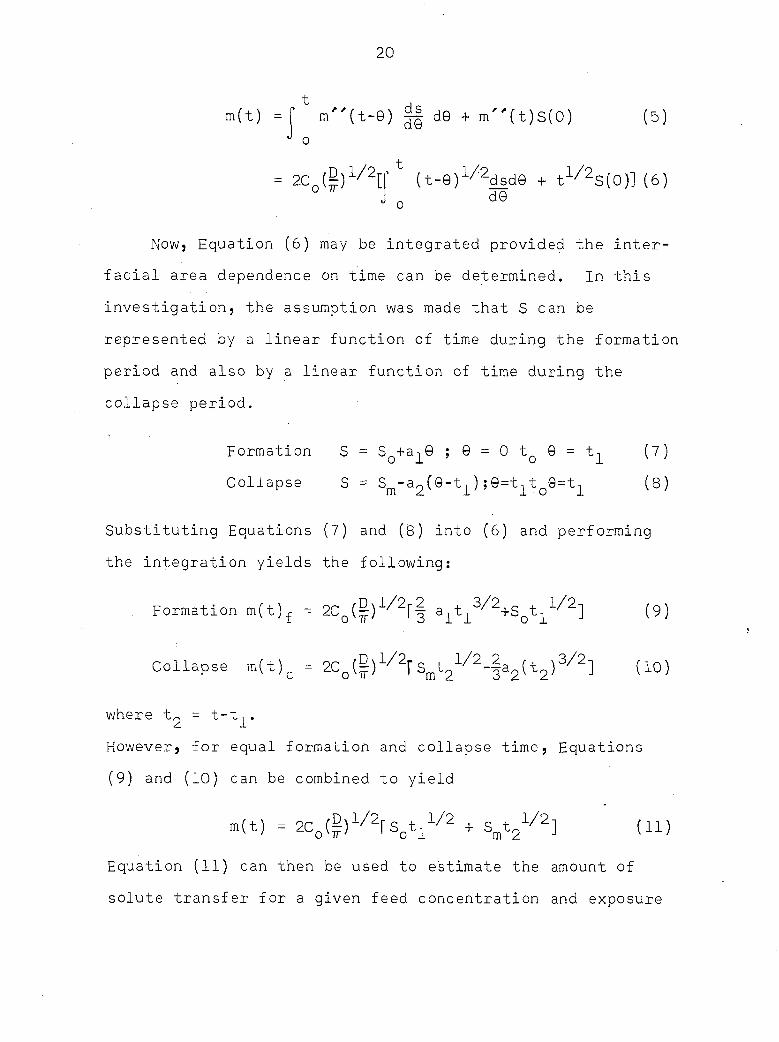
t , m(t) = f m"(t-9) d0 + m"(t)S(0) (5)

= (t-8)^d^d8 + tl/2s(0)](6) d8

Now, Equation (6) may be integrated provided the inter-

facial area dependence on time can be determined. In this

investigation, the assumption was made that S can be

represented by a linear function of time during the formation

period and also by a linear function of time during the

collapse period.

Formation S = S^a-^Q ; 6 = 0 tQ 9 = t-^ (7)

Collapse S = 2^-a^(9-t^) ;9=t^t^9=t^ (8)

Substituting Equations (7) and (8) into (6) and performing

the integration yields the following:

Formation m(t)^ = a^3/2+g^l/2-] (g)

Collapse m(t)^ = 2C^(^)l/2[s^t^/2-^a^(t2)^/2] (10)

where tp = t-t^.

However, for equal formation and collapse time, Equations

(9) and (10) can be combined to yield

m(t) = 2Co(|p)l/2r8^^1/2 + (n)

Equation (11) can then be used to estimate the amount of

solute transfer for a given feed concentration and exposure

21

time assuming a molecular dif fusional process to hold.

Model II--Surface Renewal

Danckwerts (3) and Kishinevsky (16), in dealing with

gas absorption, were the first to.present the concept of a

surface renewal mechanism for interphase mass transport.

Their ideas have been extended in attempting to investigate

models for liquid-liquid extraction processes.

For this investigation, consider transfer from a station­

ary droplet with a circulation pattern as given in Figure 1.

This flow pattern could result from viscous forces as the

continuous phase flows past the droplet or be produced by

the momentum of the fluid entering the droplet during the

formation period. As a result of this flow pattern, the

surface elements will travel with a tangential velocity,

, with transfer taking place from each of the surface

elements as they travel down the sides of the droplet.

If the assumption is made that a penetration theory

mechanism holds for transfer from each of the surface elements,

and that new surface is created as needed from the bulk of

the drop, it is possible to develop a relation for the solute

transfer from a given surface element. By summing the trans­

fer from all surface elements as the droplet is forming and

collapsing, the total solute transfer during the exposure of

the droplet to the continuous phase can be calculated. In a

later section, the following relationship is developed for

22

Figure 1. Internal circulation pattern as proposed in Model II

23

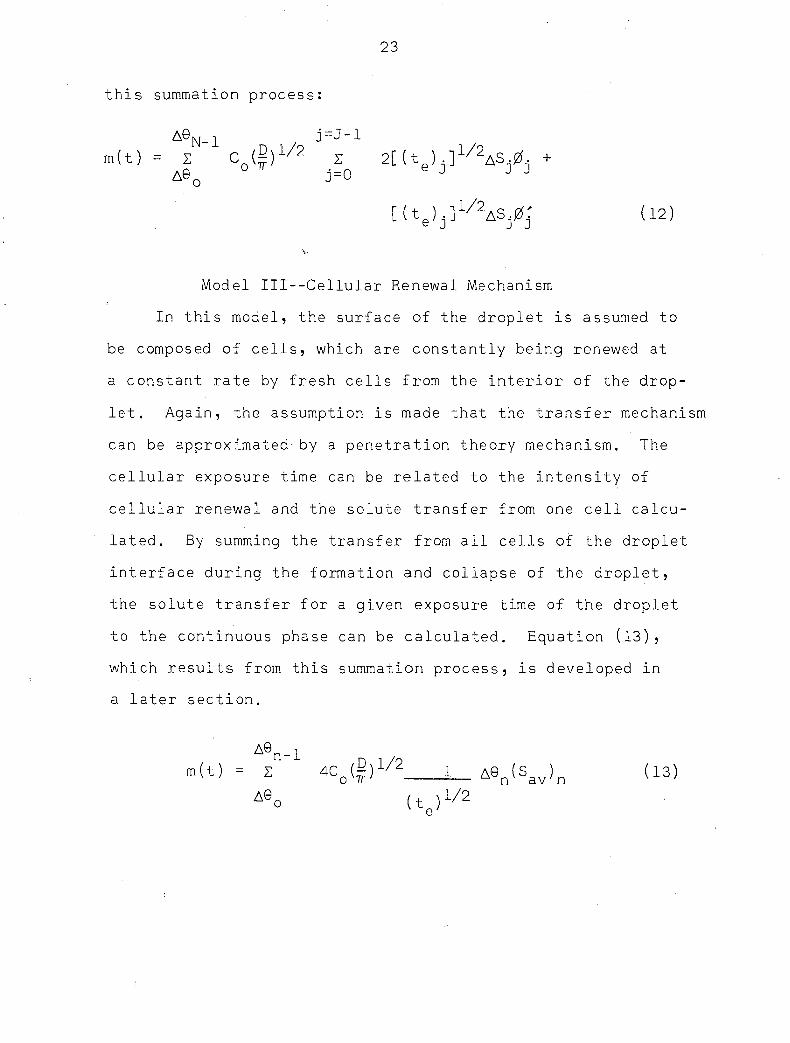
this summation process :

A6N-1 m( t ) = Z

j=J-l

j = 0

(12)

Model III--Cellular Renewal Mechanism

In this model, the surface of the droplet is assumed to

be composed of cells, which are constantly being renewed at

a constant rate by fresh cells from the interior of the drop­

let. Again, the assumption is made that the transfer mechanism

can be approximated- by a penetration theory mechanism. The

cellular exposure time can be related to the intensity of

cellular renewal and the solute transfer from one cell calcu­

lated. By summing the transfer from all cells of the droplet

interface during the formation and collapse of the droplet,

the solute transfer for a given exposure time of the droplet

to the continuous phase can be calculated. Equation (13),

which results from this summation process, is developed in

a later section.

n-1 n 1/9 m(t) = I 40^(^)1/2 1- A8n(Sav)n ( 1 3 )

24

SYSTEM

A liquid-liquid system which formed very large organic

droplets was chosen for this study. Previous investigators

had encountered difficulty in trying to use small droplets

because the change in transfer which occurred as the variables

were changed was often of the same magnitude as the experi­

mental error. This meant that whether an actual variation in

mass transfer took place was sometimes open to question. The

drop sizes used in the present work were much larger than those

which would be found in extractors, but on the other hand, the

differences in transfer rates at various operating conditions

were great enough that the observed changes could not be

attributed to experimental error.

After a preliminary investigation of several possible

systems the combination of mineral oil-propionic acid-water

was selected because large droplets could be formed and the.

distribution coefficient strongly favored the aqueous phase

at low acid concentrations. Thus, the major resistance to

mass transfer was in the organic droplet phase and only the

resistance inside the droplet was considered in the mathemat­

ical treatment of the data.

Analysis for propionic acid in the organic phase involves

a nonaqueous titration employing sodium methoxide as a titrant

and a benzene-methanol solvent. The details of the analytical

procedure can be found in reference (7).

K> Ui

WT. % ACID IN AQUEOUS PHASE

Figure 2. Distribution curve for the system mineral oil-propionic acid-water temperature 25°C

26

Table 1. American White Oil No. 21 USP

Batch no. 5881

Average molecular weight 420

% carbon in naphthene rings 38

Average no. of naphthene rings 2.5

Average no. of aromatic rings 0

% carbon in paraffin structure 59.5

.Mineral oil, rather than being a pure component, is a

mixture. The mineral oil used in this investigation was

American White oil No. 21 USP (see Table 1).

All three mathematical models treated in this investiga­

tion required values of mass diffusivity in the droplet phase,

and no experimental values of diffusivity could be found for

propionic acid diffusing in mineral oil. Therefore, an

estimation of the diffusivities was made employing a correla­

tion presented by Wilke and Chang (33). These authors present

a correlation for diffusion coefficients in the liquid phase

which is good for dilute .solutions of nondissociating solutes.

The correlation is for two component systems, but considering

the mineral oil as a single component, rather than a mixture

of similar chemical species, an estimate of the diffusivity

was made.

Deionized water was used as the continuous phase during

27

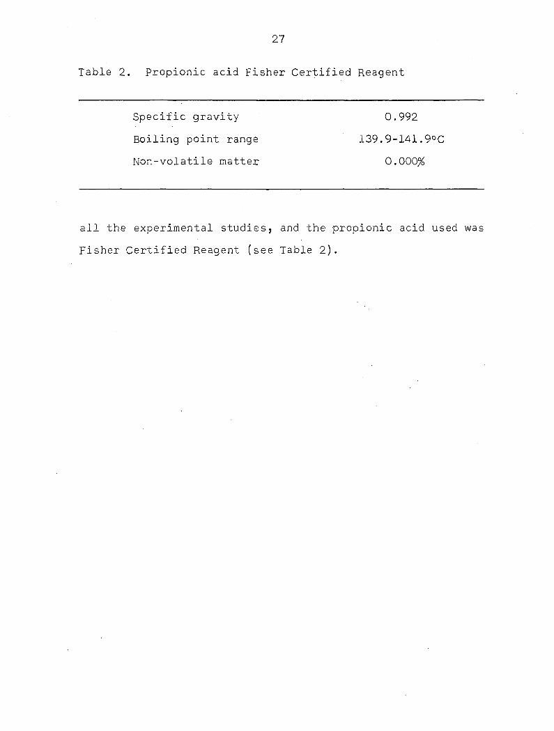
Table 2. Propionic acid Fisher Certified Reagent

Specific gravity 0.992

Boiling point range 139.9-141.9°C

Non-volatile matter 0.000%

all the experimental studies, and the propionic acid used was

Fisher Certified Reagent (see Table 2).

28

EXPERIMENTAL APPARATUS

Droplets were formed on the end of a stainless steel

drop formation tube mounted in the bottom of a three inch

square column shown in Figure 3. The column was eighteen

inches high and had a ten inch calming section in which

perforated plates were mounted to reduce the turbulence of

the continuous phase as it entered the column. Photographs

of the column are given in Figures 4 and 5.

During experimental runs, a series of organic droplets

was formed on the tip of the drop formation tube by intro­

ducing the organic phase through a feed line and into the

annulus of the drop formation tube. After the drop was formed,

it was withdrawn into a separate channel and subsequently

rejected out of column for analysis. A series of twenty to

forty droplets was formed and collapsed at a given rate with

mass transfer taking place during the exposure of the droplet

to the aqueous phase.

The flow rate of the continuous phase past the droplet

was maintained with a constant head tank, controlled with a

needle valve in the continuous phase outlet line, and measured

by a rotameter placed in the outlet line. By passing the inlet

line through coils immersed in a constant temperature bath,

the.temperature in the column was held to 25 + 1.0°C.

29

O'RING SEAL

CONTINUOUS PHASE

INLET

AQUEOUS =B-PHASE

OVERFLOW

PERFORATED

VENT

PLATE

'0 RING SEAL

PLEXIGLAS COLUMN

DROP FORMATION TIP

ORGANIC PHASE INLET

NEEDLE VALVE

SOLENOID VALVE

f-NEEDLE VALVE to* RING SEALS /////////

SCREW (ZZZZZZZZZZ

{AQUEOUS PHASE OUTLET

SOLENOID VALVE

Figure 3. Experimental apparatus

Figure 4. Photograph of the column and associated equip­ment

Figure 5. Photograph of the drop formation tube

33

34

For the experimental studies, a constant volume rate of

introduction and withdrawal of the organic phase was necessary.

A buret with a large chamber attached to its top was used as

the organic phase feed reservoir. Since only a small amount

of organic phase was used for each run, the level of liquid

in the large reservoir changed only slightly, and the head

was essentially constant. The constant head of the continuous

phase served to reject the droplet out of the apparatus.

Organic phase flow rates were controlled by micrometer-handle

needle valves in the feed and withdrawal lines.

An electronic controller which operated solenoid valves

in the feed and withdrawal lines served to fix the formation

and collapse time of the droplet. During droplet formation,

the controller opened the feed valve while closing the with­

drawal valve, and the droplet was formed. The feed valve was

then closed, the withdrawal valve opened, and the droplet

rejected from the apparatus. The controller automatically

repeated this sequence, forming a series of droplets at given

formation and collapse times. Formation and collapse times of

1 to 170 seconds were available with a precision of 0.2 per

cent.

To form large droplets of uniform size, it was necessary

to treat the drop formation tube so that the organic phase

would wet the entire tip of the tube. This was done by coat­

ing the tip with a thin polyethylene film. A hot solution of

polyethylene in xylene was prepared, the tip coated with the

35

solution, and allowed to dry. This coating remained stable

for days, but eventually deteriorated. The tip was therefore

recoated before each series of runs. Complete rejection of

the organic droplet during the collapse period was a problem.

Therefore, a five degree taper was put on the tip of the

tube to enhance the drop rejection process. Good operation

of the equipment was obtained when only a very thin film of

the organic phase remained on the tip of the tube when the

droplet was rejected.

Interfacial area and drop volume are functions of time in

the forming and collapsing drop. These quantities were

measured photographically by taking sequence photographs at

known time intervals as the drop formed and collapsed. Under

given conditions of feed concentration, formation and collapse

time, and drop size, the interfacial area and drop volume rela­

tionships with respect to time were assumed to be constant

for an entire serie.s of droplets, and photographs were made

for only one or two droplets in the series as they formed and

collapsed.

The sequency photographs were taken with a Kodak Cine

Special II 16 mm camera equipped with a 50 mm f 1.9 lens.

A description of the camera drive is given in reference ( 5 ) .

However, the camera was used without the interval timer by

simply holding the relay operated ratchet open and allowing

the camera to be driven at five frames per second. During the

latter stages of the investigation, a number of photographs

36

of the interfacial conditions during mass transfer were made.

For these photographs, a Linhof Super Technika IV with a

Ziess 40 mm macro-lens was used. Illumination was provided

by an electronic flash unit with an exposure time of 1/1000

second.

37

EXPERIMENTAL PROCEDURE

Cleanliness of the experimental equipment was an impor­

tant factor in obtaining reproducible data. Before starting

a given experimental run, the equipment was cleaned in the

following manner. All stainless steel parts, except the

needle valves, were treated twice with hot trichloroethylene

to remove any oil remaining from the previous run, allowed to

dry, and then rinsed with deionized water. The plexiglas

column and all Buna-N rubber parts were cleaned with a deter­

gent solution to remove any oil, and then thoroughly rinsed

with a large quantity of deionized water. The needle valves

were flushed with methyl alcohol and distilled water and allowed

to dry. All glassware parts were.cleaned with trichloroethyl­

ene, dichromate cleaning solution, and deionized water. When

all parts were clean and the tip of the formation tube was

coated with a polyethylene film, the equipment was assembled

as shown in Figures 3 and 4.

Before filling the column with the continuous phase, it

was necessary to introduce the organic phase into the forma­

tion and withdrawal lines. If the continuous phase entered

these lines, a long purge was necessary to remove the water

before the experimental studies could be started. It was also

necessary to coat the tip of the formation tube with the

organic phase before any of the continuous phase touched the

tip to insure complete wetting of the organic phase on the

38

tip. Once the tip had been coated with the organic phase and

the formation and withdrawal lines were filled with the

organic phase, the continuous phase was introduced into the

column. The aqueous flow rate was then set and the column

allowed to reach constant temperature.

In all experimental data an equal formation and collapse

time was used. The times were fixed on the controller and the

two needle valves adjusted to give the proper maximum drop

size within the fixed formation and collapse time. Drop sizes

were measured by observing the maximum height of the droplet

when sighting between a scribe mark on one side of the column

and a scale on the other. A traveling microscope was used to

check the droplet height throughout the experiments.

Proper operation of the equipment required that the drop­

let be completely rejected into the withdrawal line, leaving

only a thin coating of the organic phase on the tip of the

drop formation tube. Poor adjustment of the equipment resulted

in either a residual droplet remaining on the tip of the tube

or water being rejected into the withdrawal line. Both condi­

tions required readjustment of the valves and formation of

about ten droplets to purge the withdrawal line.

When the column was at constant temperature, the contin­

uous phase flow rate set, and the droplets forming to the

proper size in the given formation and collapse time, sampling

was begun. A series of about six to eight droplets were formed

under the above conditions before the organic phase was sampled.

39

Four to ten samples were then taken, with each sample con­

taining from two to four droplets, depending on the feed con­

centration. For high feed concentrations two droplets per

sample were taken while for low feed concentrations' three and

sometimes four droplets per sample were taken. Sample weights

generally were kept between 0.6 and 1.0 grams, the smaller

samples being used at the higher feed concentrations. All

samples were examined for the presence of water. "Any water

noted in the sample caused its concentration to be doubted

or disregarded in the analysis of the data.

In early work, it had been shown that solute evaporation

with small sample sizes caused an error in the analysis.

Therefore, all samples were taken in narrow neck Erlenmeyer

flasks with ground glass stoppers. After sampling, they were

immediately weighed and dissolved in 20 ml of a two to one

benzene-methanol solution in preparation for titration. This

procedure was carefully checked and shown to give reliable

results.

After the samples had been taken and processed, the

column was purged under a high continuous phase flow rate for

approximately ten minutes to remove any traces of solute from

the. continuous phase.

During the latter runs of the investigation, notes on

the interfacial condition of the droplets were taken. • Each

droplet was examined for interfacial activity or turbulence

during the transfer process. Excellent observations could be

40

made using the traveling microscope. The activity was also

visible to the naked eye. Correlation of the interfacial

condition of the droplet with the sample in which this drop­

let was rejected was difficult due to the holdup of. the organic

fluid in the withdrawal line. However, by knowing the approxi­

mate holdup volume and the drop volume, a notation of the

droplet interfacial conditions with the sample in which the

droplet was rejected could be made.

41

DESCRIPTION OF MASS TRANSFER MODELS

Three proposed models for the mass transfer process in a

forming and collapsing droplet were studied. These models

were :

The assumptions and essential features of Model I have been

discussed previously. In both Models II and III a method to

generate the volume and interfacial area of the droplet as a

function of time was necessary. The shape of the droplet was

represented by a paraboloid of revolution, and this paraboloid

could be considered to grow and collapse as the droplet was

exposed to the continuous phase.

The method of generating the paraboloid•as. a function of

time was as follows. Consider that the volume of the paraboloid

increases at a constant rate due to a constant flow rate of the

organic phase into the droplet. The volume also decreases

linearly during the collapse period due to a constant flow rate

of organic phase out of the droplet. Therefore :

Model I Molecular Diffusion Mechanism Model II Surface Renewal Mechanism Model III Cellu.lar Renewal Mechanism

9 = 0 to 0 = t1

9 = t-^ to 9 = t

(14)

(15)

where

42

a = rate of introduction of organic phase, or rate of withdrawal

tj - formation time,

t = total exposure time,

tj = t-t^ (equal formation and collapse time),

9 = time,

V = droplet volume,

V = maximum droplet volume.

Assume that the droplet height, k, during both the formation

and collapse periods can be represented by linear function of

time.

The assumptions that both k and V were linear functions of time

were checked by calculations from sequence photographs taken

during the experimental runs and were found to be reasonably

good.

The equation for a parabola as shown in Figure 6 is

However, if this parabola is revolved 180 degrees about the z

axis, a paraboloid of revolution is generated with volume and

surface area given by

9 = 0 to 9 = t-^

9 = t^ to 9 = t

(16)

(17)

y2 = -2p(z-k) (18)

V = TTpk2 (19)

(20) s - [(p2 + 2pk)3//2-p3]

43

Equations (19) and (20) were confirmed in the following refer­

ences respectively (8, 15).

If V and k are known functions of time, p may also be

determined as a function of time from Equation (19). With k

and p determined, the interfacial rea, S, can be calculated

from Equation (20). and km can be determined from the

sequence photographs of the droplet as it forms and collapses.

For equal formation and collapse time, a and a, can be deter­

mined from the following expressions:

Hence, by knowing and km for a given exposure time, S and

V can be calculated at any given value of 9 during this exposure

time.

Model II, a surface renewal model, incorporates the

assumption that the mass transfer process may be approximated

by a penetration theory mechanism from elements of surface

which are constantly being renewed from the bulk of the drop­

let. Under certain conditions Equation (4) may serve as a

good approximation to the mass transfer for (a) liquid layers

of restricted depth, and (b) liquid moving parallel to the

surface with a velocity that varies with depth. Danckwerts

(3) states, "The necessary condition for (a) is that the time

av = VmZtl ( 2 1 )

(22)

Model II

44

of exposure should be so short that the depth of penetration .

is less than the depth of the liquid; for (b) it must be so

short that the depth of penetration is less than the depth at

which the velocity is appreciably different from that at the

surface." Condition (b) is assumed in this model and therefore

Equation (4) serves as the basis of Model II.

Consider a droplet as it forms and collapses. Assume

that during both the formation and collapse period the internal

circulation pattern may be represented by the flow pattern

given in Figure 1. Further, assume that mass transfer takes

place from elements of surface as they travel down the droplet

with a tangential velocity, v^.

The amount of solute transfer during a given exposure

time, t, may be estimated by the following incremental proce­

dure. First, divide the exposure time into an even number of

increments, N. - :

A@ = t/N (23)

where

= ®1 - ®o' ' ' = ®n+l"®n'" ' " &®N-1

= ®N"®N-1

By the following steps, the amount of solute transferred during

a given time increment, A®ns can be calculated:

(1) Calculate the following :

If ©n < t/2 (Formation Period)

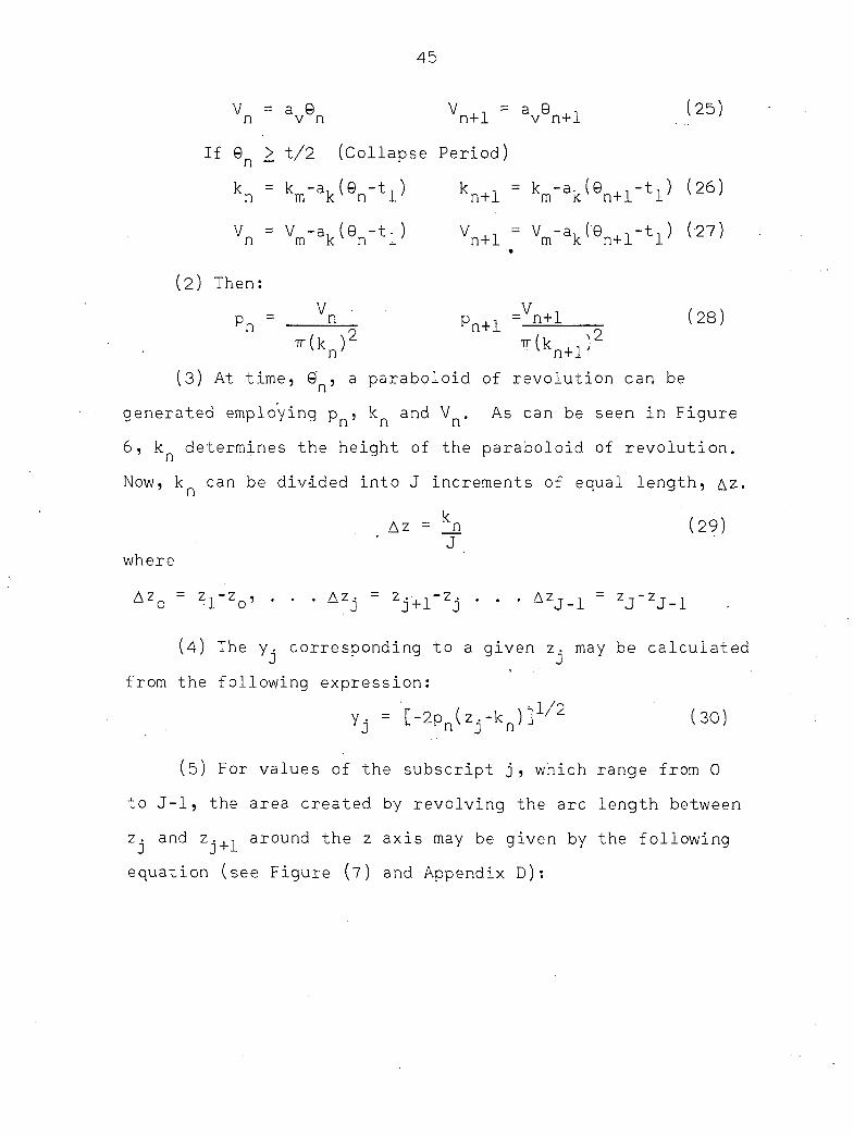
45

Vn = avSn Vn+1 = avSn+l (25)

If 9n > t/2 (Collapse Period)

kn = km-ak(0n"tl) kn+l = V^n+rV (26)

Vn = \-\{en-hî Vn+1 <27>

(2) Then :

Pn = X? Pn+1 5 (28)

T(kn' r(kn+l'

(3) At time, 0 , a paraboloid of revolution can be

generated employing pn, and V . As can be seen in Figure

6, kn determines the height of the paraboloid of revolution.

Now, kn can be divided into J increments of equal length, &z.

Az = ^n (29) J

where

Azo = zl"zo' ' * ' Azj = Zj+l~Zj " * ' AZJ-1 = ZJ"ZJ-1

(4) The yj corresponding to a given Zj may be calculated

from the following expression:

Yj = [-2P^(Zj-k^)]l/2 (go)

( 5 ) For values of the subscript j, which range from 0

to J-l, the area created by revolving the arc length between

Zj and Zj+-L around the z axis may be given by the following

equation (see Figure (7) and Appendix D):

46

Z

y = -2p(z-k)

Figure 6. Parabola with vertex at z = k and y = 0

Z

Yi

Figure 7. Parabola showing notation for Model II

47

<sj>en = % [(Pn2+2Pnkn-2Pnzj )3 /2- (Pn2+2Pnkn-2Pnzj+l'3/2l

( 3 1 )

(6) An expression similar to (31) can be developed

repeating steps (3), (4) , and (5) for time ©n+j_

^®n+l ̂ %î+î +2Pn+lkn+l"2Pn+lZj)^

^pn+l+2pn+lkn+l"2pn+lzj+l^ ̂

( 3 2 )

(7) The average area exposed to the continuous phase

during A®n is

( S ) , = ( S j ' e n + ' S j ' % l ( 3 3 ) av

2

(8) Also, for values of the subscript j ranging from 0

to J-I5 the arc lengths between Zj and + may be calculated

for ©n and 9n+j_ (see Appendix D) .

(Ven ' 2^ [ Yj (yj+pn'1/2"Yj +1(Yj+1 +Pn'1/2^

+ P n 1 r V ( Y t + P n > V 2 1 ( 3 4 )

2 Yj+i+(y2+i+p2)^2

(Lj'en+1 = 2iT- ryj tYj+p2+l )1 /2"yj+l tyk+Pn+l )1 /2 ]

n x pn+l

+ p n + l l n r V ' V P n ' 1 ( 3 5 )

2 yj+l+^j+l+Pn)1/2

(9) The average arc length between Zj and zj+]_ during

A0n is therefore

48

( k-i ) © + ( L. ) g

(Yav = ^^

(10) For ©n and 9n+1 calculate (Sj)av and (L^)ay for j

values ranging from 0 to J-l yielding :

(So)av'

^L0^av' ^Ll^av' ' * ''^Lj ̂av' * " 1>^LJ-l^av,

(11) Now, the top area increment of the droplet,

(Sj_^)av, will travel down the paraboloid with a velocity,

v_j_, and hence its exposure time will be

j=J-l

(Lj)av

(t )T , _ Total Arc Length _ ^ ^ (37)

(12) However, as (S.j_]_)av travels down the droplet, new

interfacial area must be created from the bulk of the droplet,

since the area cut by the j subscripts increases as you pro­

ceed down the droplet. The increase in interfacial area in

going from (S^)ay down to (S^ _1)av is

&Sj = (S j . V a v - < S j>av ' 3 8 '

This new interfacial area will have an exposure time, (tg)^,

given by

(te>j = ^ J0

( L j ) av / V t ( 3 9 >

(13) If a penetration theory mechanism is assumed for

the transfer process from each of the surface elements as they

49

travel down the droplet, the following equation may be used

to estimate the amount of solute transferred from a unit

surface element.

m" = 2Co(V)1/'2 (40) TT

Equation (40) is equivalent to Equation (4) with (t-9) = (tg).

Therefore, the same assumptions and boundary conditions given

for (4) hold for (40).

(14) Consider now the transfer of solute from (Sj_^)^

as it travels down the droplet. The amount of solute trans­

ferred in A9n is

^mJ-l^A0n = 2Co^7T^1//'2^te^J-l-'1//2^SJ-l^av ^1)

(15) The amount of solute transferred from a new surface

element that must be created between j values of j and j-1

as (Sj_-^)av travels down the droplet is

(mAen = (42)

(16) All surface elements that start at the top of the

droplet require a time, (tg)j_j_ ? to reach the base of the

droplet. However, when 9 > @n~(te)j_j, an element of surface

will not have sufficient time to reach the base of the drop­

let. The number of surface elements that start at the top

of the droplet and reach the bottom in time, A©n? may be

easily determined. Let this number be 0j ̂

50

0 t i = A ® n - ( t e ) j _ l ( 4 3 )

^LJ-l'av/Vt

Similarly, the number of new surface elements between j and

j-1 that must be created in time, A®n5 which also reach the

base of the droplet is

0 . = (44)

J lLj'av/Vt

(17) Therefore, the number of area elements (A.) that J av

occur in time, A0nJ times the transfer from one of the ( Aj ) av

elements yields the contribution of this amount of surface to

the total transfer process. Summing all these contributions,

both from surface at the top of the droplet and the new

surface created further down the droplet yields the total

amount of solute transferred in time, A©n.

^ Z ̂(m.) g = ^ Z \c (§)^[(t (45) j=0 J n j = 0 J 33

This equation holds provided aSj is defined by Equation (38)

when j < J-l and by the following relation when j = J-l.

ASJ-1 = (SJ-Vav (46)

Equation (45) estimates the solute transferred in time,

A0n~(te)j_1. (Refer to step (16)).

(18) An approximation must be made when 9 > A9n~

since all surface elements starting at the top of the droplet

will not reach the base of the droplet. The transfer during

this period of time 0 > was approximated by 1/2 of

the transfer that would occur in an equal period of time

assuming conditions were the same as those in the first por­

51

tion of A®nj i.e. all elements of surface that start at a

given point on the droplet reach the base of the droplet.

Therefore, the contribution to the amount of solute transfer

during the final (te)j_j of A@n was estimated by

j=J-l j=J-l n i/o S (mO.o = S c (B)V2 [ ( t ) ] ( A S ) 0 - (47 ) j=0 3 n j=0 0 e J J J

where

0 ' . = ^ J-l (48)

(19) Adding Equations (45) and (47) yields the total

amount of solute transferred in time, A©n.

j=J-l j=J-l j=J-l T) •)/o i/o

+ JÏ0 im'^Sn ~~ j!o 2C0y

+ J .5nlco(ï)1/2[ (te) j ]1/2(ASd )0j j ̂

= c0(2)1/2 2[(te)j]1/2ASj0j+[(te)j]1/2&Sj0Jf

(49)

(20) Calculation of the transfer occurring during each

A©n5 (repeating steps.(l)—(19) with n = 0 to n = N-l) and

summation of the contributions from each of these time in­

crements yields the total solute transfer in time, t.

52

^N-l m(t) 2 Z (m.) p + (mf).A

A@o j=0 J : AW^

A@n x j=J-l

r C(5 )V2 z 2[ ( t ) ]V24S ( |K )+[(t ) .]1/2(aS )0 : A0O j=0 3 J J J 3 J

(50)

Certain restrictions must be placed on the use of

Equation (49). In step (18) it was stated that is

only an approximation to the amount of solute transferred when

8 > 8 - (tg)j_2« Equation (49) works best when

(m')AÛ « (m.) Q + (mf) Q , i.e. the approximation during J A0n J Ayn 3 n

9 > 9 - ( tg ) J_j_ ? is small in comparison to the total transfer

occurring in A©n. Examination of Equations (45) and (47)

shows that (mf) Q may be made small in comparison to (m.) Q J A«n J A«n

by making JZT large in comparison to 0 f . Substituting Equation

(39) into both (44) and (48) yields (51) and (52) respectively,

j=j Z

='A9r - (j-0(L.)av/vt) (51)

(S -V tA

j - J -1

0 f = 3 = 0 ^ L i ^a \ / V t (52)

(Lj>a/Vt

From Equations (51) and (52), it can be seen that JZL will be

large in comparison to 0f when v^ is large for a constant

value of A0n. Therefore, the model will work best for high

53

values of v^ while the error introduced with the approximation,

(mf), becomes larger as v, is decreased. J "t-

Also it should be mentioned that Equation (49) showed

a slight dependence on the value of J used in the calcula­

tions. However, as J was increased, Equation (49) approached

asymptotically a constant value of m(t).

Equation (49) was used to calculated the amount of solute

transferred under conditions of different exposure times and

three feed concentrations. Calculations were carried out on

an IBM 7074 digital computer with a time increment, A©n? of

2 seconds and a J value of 100.

Model III

Model III, a cellular renewal mechanism involves the

assumption that the droplet surface is composed of cells,

which are constantly being renewed by fresh cells from the

interior of the droplet. Further, the assumption is made

that the mechanism of solute transfer from the cells can be

approximated by a penetration theory mechanism. As was the

case in Model II, Equation (4) serves as a good approximation

to the solute transfer process provided the time of exposure

of the cells to the continuous phase is short.

Interfacial area and drop volume can then be generated

in the same manner as for Model II. Assume k and V to be

linear functions during the formation and collapse of the

droplet and from these two quantities generate S as a function

54

of time.

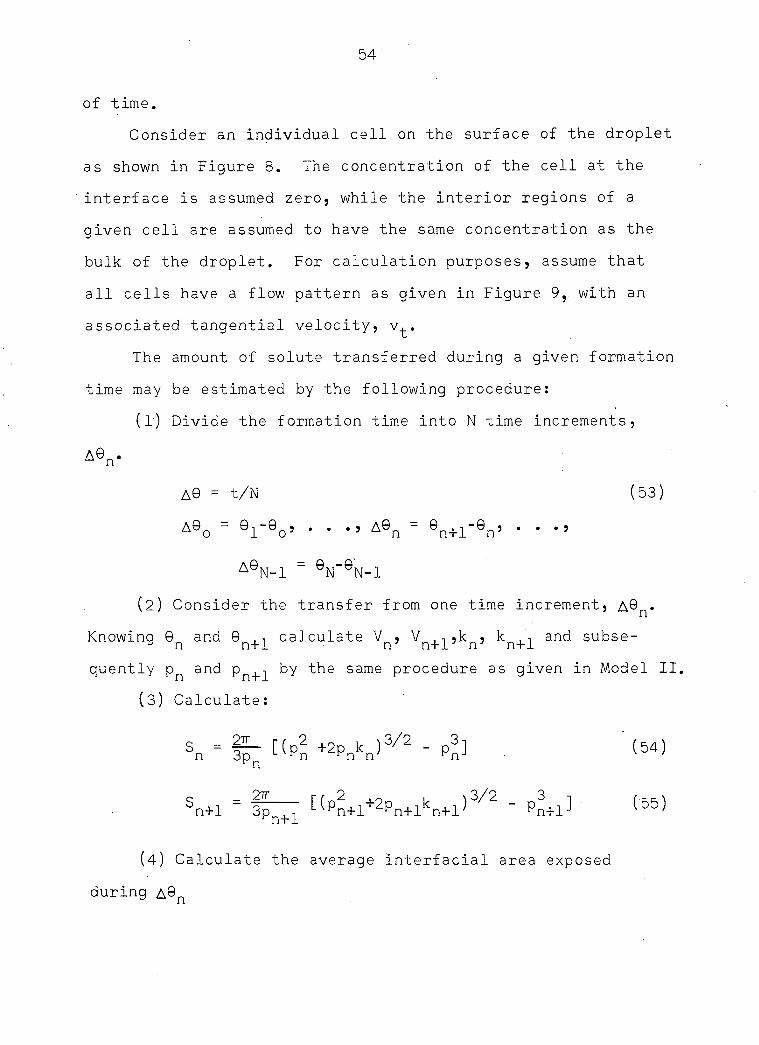
Consider an individual cell on the surface of the droplet

as shown in Figure 8. The concentration of the cell at the

interface is assumed zero, while the interior regions of a

given cell are assumed to have the same concentration as the

bulk of the droplet. For calculation purposes, assume that

all cells have a flow pattern as given in Figure 9, with an

associated tangential velocity, v^.

The amount of solute transferred during a given formation

time may be estimated by the following procedure:

(l) Divide the formation time into N time increments,

(2) Consider the transfer from one time increment, A©n«

Knowing ©n and ©n+j_ calculate V^, Vn+^,kn, kn+j_ and subse­

quently pn and Pn+j_ by the same procedure as given in Model II.

(3) Calculate :

A© = t/N (53)

A®o - ®l"®o' ' ' " " ®n+r®n' ' " " n+1 n

A®N-1 - ®N"®N-1

(54)

( 4 ) Calculate the average interfacial area exposed

during A@n

55

Z

Figure 8. Droplet surface showing one cell of dimensions, and for Model III

LIQ.-LIQ. INTERFACE

*

v,i AQUEOUS

PHASE

ORGANIC PHASE W2

t c=o

1 c=c,

Figure 9. Flow pattern of cells in Model III

56

(Sav)n = Sn * Sn+1 (56)

(5) The cellular exposure time, t , for all cells over

the droplet is given by

tg = (57)

(6) Let the number of times a cell such as the one given

in Figure 9 is renewed be R. Then

R = &9n (58)

*6

( 7 ) The amount of solute transferred from one cell of

dimensions 1/V^ and during an exposure time, te, assuming a

penetration theory mechanism is given by

m = 2C^(^) 2̂(tg)^(W^) (59)

(ô) The total solute transfer from the average area of

the droplet exposed during a time A©n is

(m) - = 2C (g)l/2(t )l/2(ww )(R)(favln (60) n 0 7r

' e 12

(9) With this model the amount of solute transferred

during the formation period is equal to the amount of solute

transferred during the collapse period, since the formation

and collapse processes are symmetrical. The total transfer

of solute is then calculated by summing the transfer during

each A©n for the formation period and multiplying by a factor

of two to account for the collapse period.

57

m(t) = Z* (£)1/2 ( t )1/2 (W,W_ )R(61) A9q ° e 12 TW^T

Substituting Equation (58) into (61) and simplifying yields

A@N-1 _ m ( t ) = Z 4 C ^ ( : ) : / 2 _ J _ ^ ( S ^ ) ^ ( 6 2 )

Equation (62) can now be used to estimate the transfer ' 9

from a forming and collapsing droplet under different condi­

tions of exposure time and feed concentrations. Calculations

were again carried out on an IBM 7074 digital computer with a

A@n of 2 seconds.

58

RESULTS

Interfacial Turbulence

Often spontaneous interfacial turbulence or activity

occurs during liquid-liquid mass transfer studies. This

activity, if undetected, can cause wide discrepancies in mass

transfer data. Previous investigators reported increases in

the rate of transfer when interfacial turbulence was present.

Although several theories have been proposed to explain the

origin of interfacial activity, little quantitative informa­

tion is known about the phenomena.

Interfacial activity or turbulence was frequently

observed during the mass transfer studies on the forming and

collapsing droplets. Evaluation of the interfacial condition

of the droplet was often difficult since the degree or inten­

sity of the interfacial activity was not always the same.from

one droplet to another. Frequently, interfacial activity was

absent until the droplet reached approximately one half of

its maximum volume, at which time very vigorous activity

occurred. This activity remained for the rest of the forma­

tion period and damped out as the droplet collapsed. Inter-

facial activity was often present only on localized areas of

the droplet interface, particularly in regions near the top

of the droplet.

Photographs of the droplet with turbulent interfacial

conditions are presented in Figures 10 and 11, and a photo-

f

Figure 10. Photograph of droplet with interfacial activity present

Propionic acid transferring out of a mineral oil droplet into a water phase

Feed concentration 14.6 wt. % acid

Tip diameter 0.962 cm.

60

Figure 11. Photograph of droplet with interfacial activity present

Propionic acid transferring out of a mineral oil droplet into a water phase

Feed concentration 14.6 wt. % acid

Tip diameter 0.962 cm.

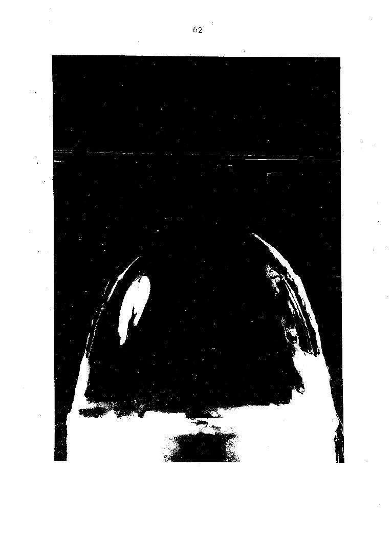
63

graph of nonactive interfacial conditions is presented in

Figure 12.

Sternling and Scriven (26) have proposed a simplified

model to explain the origin of interfacial turbulence between

two unequilibrated liquids. From an analysis of their model,

they suggest that interfacial turbulence is usually promoted

by the following eight conditions :

(1) solute transfer out of the phase of higher viscosity

(2) solute transfer out of the phase in which its

diffusivity is lower;

(3) large difference in kinematic viscosity and solute

diffusivity between the two phases ;

( 4 ) steep concentration gradients near the interface;

(5) interfacial tension highly sensitive to solute

concentration;

(6) low viscosities and diffusivities in both phases;

(7) absence of surface-active agents; and

(8) interfaces of large extent. i

In this investigation all conditions proposed by Sternling

and Scriven were present during the mass transfer studies

except possibly conditions (4) and (6), although condition

(4) was probable in view of the low diffusivity of the acid

in the droplet phase, particularly when the droplet exposure

time was short. In view of the conditions proposed by Stern­

ling and Scriven, it was reasonable to expect interfacial

activity during the transfer studies.

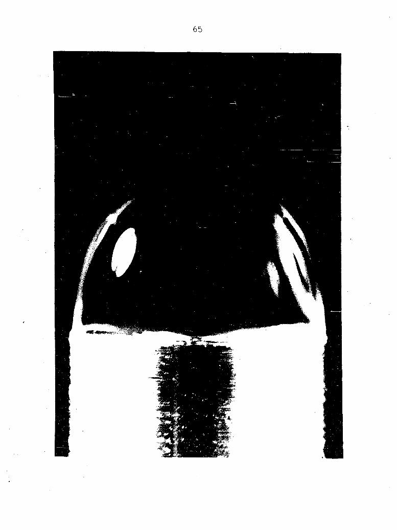
Figure 12. Photograph of droplet with nonactive interfacial conditions

Propionic acid transferring out of a mineral oil droplet into a water phase

Feed concentration 14.6 wt. % acid

Tip diameter 0.962 cm.

65

66

Experimental data were obtained for three levels of feed

concentration, 9.8, 14.6, and 19.5 weight per cent acid and

are tabulated in Appendix A. The data taken at a feed con­

centration of 9.8 weight per cent acid were the most consis­

tent data of the three levels of concentration investigated.

Data scatter was encountered in experimental results for

the two higher feed concentrations. Increasing the feed con­

centration would enhance Sternling and Scriven's conditions

(4) and (5). Therefore, it would be reasonable to expect more

erratic interfacial activity and consequently more scatter in

the experimental data.

Experimental Results

Experimental data were taken for three levels of feed

concentration and for droplet exposure times ranging from ten

to sixty seconds. In all cases an equal formation and collapse

time was used with a drop size of approximately 0.31 cc.

Figure 13 is a plot of per cent acid remaining in the

droplet versus droplet exposure time for a feed concentration

of 9.8 weight per cent acid. Two curves are presented, one

for nonactive interfacial- conditions (white data points) and

one for turbulent or active interfacial conditions (black

data points). Both curves gradually decrease with increasing

exposure time. A substantial increase in solute transfer

occurred when interfacial turbulence was present as seen by

the difference in ordinates of the two curves at a given

100

e> z z <t 2 UJ a: o o <

38

90i—

80

TURBULENT INTERFACIAL CONDITIONS

O

Figure 13,

10

/NONACTIVE e1 INTERFACIAL O CONDITIONS

o

50 60 20 30 40 EXPOSURE TIME, SECONDS

Per cent acid remaining in.the droplet versus total exposure time of the droplet to the continuous phase (experimental Runs G-9, G-10, and G-ll, f e e d c o n c e n t r a t i o n 9 . 8 w t . % a c i d , a v e r a g e d r o p l e t v o l u m e 0 . 3 1 c c . )

68

exposure time.

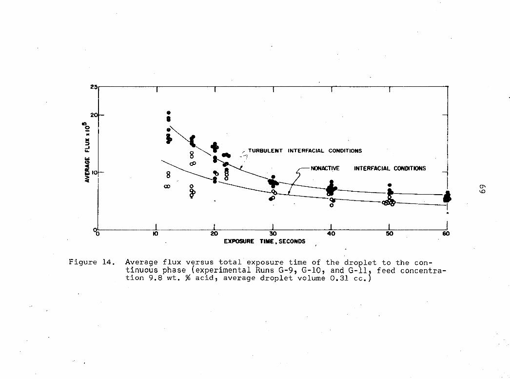
Figure 14 is a plot of average flux, i|), versus exposure

time for a feed concentration of 9.8 weight per cent acid.

The average flux represents the grams of acid crossing a unit

interface in unit time. Since interfacial area was a func­

tion of time, an average area was used to calculate the flux

quantity;

tJ, = Grams acid transferred (63)

(VSm> x t 2

In Figure 13, a higher flux for a given exposure time re­

presents increased transfer and again increased transfer due

to interfacial activity was found. Average flux is useful

for comparison of experimental results with different feed

concentrations, since per cent acid remaining has little sig­

nificance when attempting to compare data with different feed

concentrations.

Data taken at the two higher feed concentrations showed

trends similar to those in Figures 13 and 14. A decrease in

per cent acid remaining with increased exposure time was ob­

served along with an increase in transfer due to interfacial

activity. At low exposure times, increasing the feed concen­

tration resulted in increasing the average flux quantity with

other conditions held constant. At long exposure time, the

variation of average flux with concentration was not well

defined.

25

TURBULENT INTERFACIAL CONDITIONS

NONACTIVE INTERFACIAL CONDITIONS w «O

CD

20 30 EXPOSURE TIME,SECONDS

40 50 60

Figure 14. Average flux versus total exposure time of the droplet to the con­tinuous phase (experimental Runs G-9, G-10, and G-ll, feed concentra­t i o n 9 . 8 w t . % a c i d , a v e r a g e d r o p l e t v o l u m e 0 . 3 1 c c . j

70

On a number of experimental runs the effect of the con­

tinuous phase flow rate past the droplet on the solute trans­

fer was investigated. Initial expectations were that an

increase in the continuous phase flow rate would increase

the amount of solute transfer if all other conditions were

constant. No significant dependence of the solute transfer

on the continuous phase flow rate was found. Therefore, all

subsequent data were taken at a continuous phase flow rate of

310 cc./min.

Experimental Error

During the drop formation and collapse studies, experi­

mental error was expected from two sources. The error in­

volved in the analysis of the samples, which included stand­

ardization of titrant and weighing of the samples, was esti­

mated to be less than 0.5 per cent. The error which resulted

from the operation of the equipment was significantly higher.

Due to the nature of the experiments, it was difficult

to hold drop size constant during a run, and an average

variation of five per cent in a desired drop size of 0.31 cc

was estimated. By means of Model III, the effect of a five

per cent variation in drop size on the per cent acid remaining

in the droplet was obtained. First, conditions were found

to make the model agree with experimental data for a given

formation time and a feed concentration of 9.8 weight per

cent acid. Drop size was then increased by five per cent and

71

the per cent acid remaining in the droplet calculated. By

this procedure, it was found that a five per cent variation

in drop size caused a two per cent variation in per cent acid

extracted. .

Occasionally, it was necessary to shorten the desired

exposure time to prevent water from being rejected into the

collapse line. On these occasions a maximum error of five

per cent in exposure time was possible, but usually this error

was approximately two per cent for most of the experimental

data.

An exact analysis of the experimental error involved in

the experimental studies is difficult because of interaction

among variables. For example, a slight increase in drop

volume causes an increase in interfacial area, which should

increase the mass transfer. Because of the volume increase,

however, more acid is available for transfer.

In general, it is felt that an experimental error of less

than two per cent was reasonable for most data in this inves­

tigation. Because experimental error for each observation

could not be determined accurately, a large number of experi­

mental observations were made at each point to obtain a better

i estimate of the measured quantity.

Comparison of Transfer Models

with Experimental Results

Calculations for three transfer models were carried out

on an IBM 7074 digital computer at feed concentrations cor­

72

responding to those used in the experimental portion of the

investigation. Programs for all three models are presented

in Appendix B. One drop size was investigated for exposure

times varying from ten to sixty seconds. In all computations,

an equal formation and collapse time was used.

Experimental values of droplet volume and interfacial

area determined from droplet profiles taken from sequence

photographs are plotted versus exposure time in Figures 15 and

16. The equation for a parabola was then fitted to the pro­

file, and volume and interfacial area calculated from Equa­

tions (19) and (20). The theoretical points on Figures 15

and 16 represent interfacial area and droplet volume as the

computer generated them for Models II and III. The experi­

mental data points on Figure 15 show that volume was a linear

function of time during the formation and collapse of the

droplet.

Model I incorporated the assumption that interfacial area

can be approximated by a linear function of time during both

the formation and collapse period. Experimental data points

on Figure 16 show that this assumption is reasonable.

A number of assumptions are common to all three models.

First, the assumption was made that no interphase transport

of water or of oil occurs in the droplet. Second, the con­

centration of solute at the interface of the droplet was

assumed to be zero. This assumption was made for several

reasons. First, at equilibrium conditions, the solute strongly

0.4 EXPERIMENTAL O

COMPUTER 0

0.3 -O • • O

ro . o O 0

UJ r 0.2-

o >

O •

0.1 -

D _L

0 10 20

EXPOSURE TIME, SEC.

Figure 15. Droplet volume versus t ime for an exposure t ime of 30 seconds (experimental data points from Run G-9, feed concentration 9.78 wt,

% acid)

30

CVI

2.0

1.8

1.6 o < 14 UJ o: < 1.2

< 5 l.O 2 5 0.8< H

~ 0.6

0.4

1 • « .

- O

O • O

-

o • • 1

1

D O •

O D • °

o D

DO

-

0

• 0

• 0

•

1 O—

1 I

•

O

•

0

•

EXPERIMENTAL O

COMPUTER • l i

0

Figure 16.

10 20 EXPOSURE TIME, SEC.

Interfacial area versus t ime for an exposure t ime of 30 seconds (experimental data points from Run G-9, feed concentration 9.78 wt. acid)

30

75

favored the continuous phase. The diffusivity of solute in

the continuous phase was an order of magnitude larger than in

the organic phase and therefore could be expected to diffuse

rapidly away from the droplet interface. Second, the movement

of the continuous phase past the droplet served to sweep away

any solute near the surface of the droplet. The third assump­

tion common to all three models was that the diffusing, species

in the organic phase was one molecule of propionic acid.

All three models required values of mass diffusivity.

Since experimental values were not available, diffusivities

were calculated from a correlation presented by Wilke and

Chang (33). Diffusivities obtained in this way had a possible

error of + 10 per cent.

Model I

Mass transfer results for Model I, a molecular diffusion

mechanism, are presented in Figures 17 and 18 along with

experimental data for a feed concentration of 9.8 weight per

cent acid. As may be seen in Figures 17 and 18, Model I

predicts lower mass transfer than is encountered experimental­

ly. Per cent acid remaining gradually decreased as exposure

time was increased and the average -flux behaved in the same

manner.

Tabular results for the calculations at all three feed

concentrations are presented in Appendix B. For a given

exposure time, the average flux quantity increased as the feed

100

o

< S UJ (K

5 S

MODEL I

90

TURBULENT INTERFACIAL CONDITIONS

/NONACTIVE ef INTERFACIAL o) CONDITIONS

et

-4 O

80 10

Figure 17.

20 30 40 50 < EXPOSURE TIME, SECONDS

wt. % acid, average droplet volume 0 .31 ce . ;

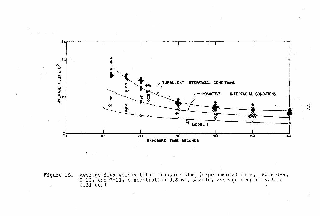
25

20

in

_i u. TURBULENT INTERFACIAL CONDITIONS

UJ o CP INTERFACIAL CONDITIONS

uj 10

CO

MODEL I

40 30 EXPOSURE TIME,SECONDS

50 60 20

Figure 18. Average f lux versus total exposure t ime (experimental data, Runs G-9, G-10, and G-l l , concentration 9.8 wt. % acid, average droplet volume 0 .31 cc. )

78

concentration was increased.

An interesting observation is possible if the assumption

is made that Model I accurately describes the contribution of

molecular diffusion to the transfer process. The mass transfer

occurring during the exposure of the droplet to the continuous

phase may then be broken into three parts:

(1) transfer due to molecular diffusion;

(2) transfer due to bulk fluid motion;

(3) transfer due to interfacial activity.

The entire transfer occurring at a given exposure time is

represented by the value of the curve at turbulent interfacial

conditions (Figure 17). The difference between the curves at

turbulent and nonactive interfacial conditions represents the

transfer due to interfacial activity. Similarly, the dif­

ference between the curves representing Model I and nonactive

interfacial conditions yields the transfer due to bulk fluid

motion. Finally, the transfer due to molecular diffusion is

represented by the curve for Model I. The contribution of

each of the three parts to the total transfer can then be

estimated in terms of the percentage of the total transfer.

Table 3 gives results for three exposure times. Although

there is a possibility of a large error in this type of cal­

culation, it is interesting to note that the contribution

from molecular diffusion increases with exposure time, while

the contribution due to fluid motion decreases with exposure

time. Low exposure times result in a high momentum of the

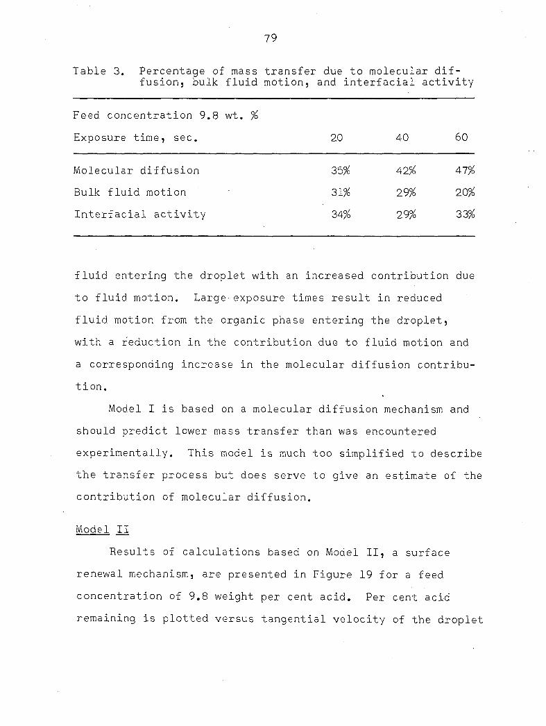
79

Table 3. Percentage of mass transfer due to molecular dif­fusion, bulk fluid motion, and interfacial activity

Feed concentration 9.8 wt. %

Exposure time, sec.

Molecular diffusion

Bulk fluid motion

Interfacial activity

20 40 60

35% 42% 47%

31% 29% 20%

34% 29% 33%

fluid entering the droplet with an increased contribution due

to fluid motion. Large exposure times result in reduced

fluid motion from the organic phase entering the droplet,

with a reduction in the contribution due to fluid motion and

a corresponding increase in the molecular diffusion contribu­

tion.

Model I is based on a molecular diffusion mechanism and

should predict lower mass transfer than was encountered

experimentally. This model is much too simplified to describe

the transfer process but does serve to give an estimate of the

contribution of molecular diffusion.

Model II

Results of calculations based on Model II, a surface

renewal mechanism, are presented in Figure 19 for a feed

concentration of 9.8 weight per cent acid. Per cent acid

remaining is plotted versus tangential velocity of the droplet

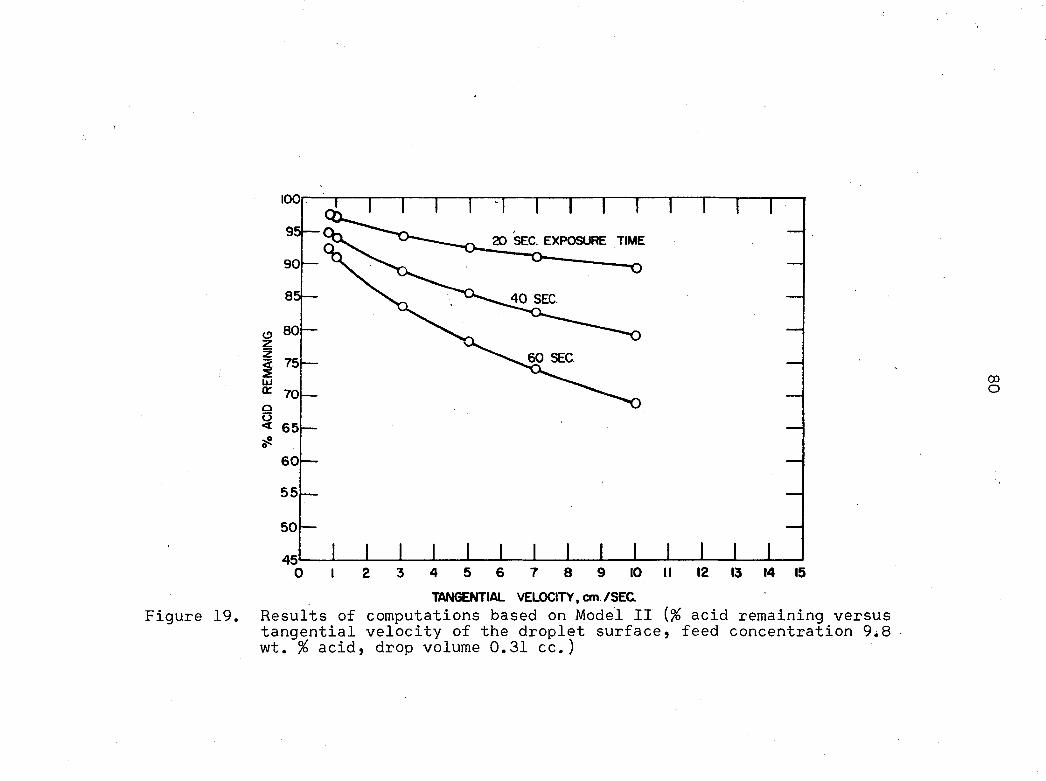
Figure 19.

20 SEC. EXPOSURE TIME

40 SEC

60 SEC

i—i—i i i i—i—r

I I I I l_l I I L

00 o

10 II 12 13 14 15

TANGENTIAL VELOCITY, cm./SEC Results of computations based on Model II {% acid remaining versus tangential velocity of the droplet surface, feed concentration 9*8 wt. % acid, drop volume 0 .31 cc . )

81

surface for three droplet exposure times. As would be ex­

pected, increasing the tangential velocity increases the

solute transfer for a given exposure time.

Results of calculations based on Model II for all three

concentration levels are presented in Appendix B. •

A good test for this model would be to determine the

dependence of the solute transfer on the tangential velocity

of the droplet. If the assumptions were made that the tan­

gential velocity of the droplet surface had the same -value

as the velocity of the continuous phase past the droplet, and

the continuous phase velocity were varied, estimates of the

per cent acid remaining in the droplet versus tangential

velocity, v^, could be made. However, a twentyfold change

in the continuous phase velocity, from 0.01 to 0.2 cm./sec.

produced no consistent trend or variation in per cent acid

remaining in the droplet. A number of possible explanations

for this result may be presented. First, the possibility

exists that interfacial turbulence was masking any dependence

that could be measured. Second, the range of variation in

continuous phase flow rate was too small to measure the de­

pendence. As seen in Figure 19, a large change in tangential

velocity was required to significantly change the per cent

acid remaining in the droplet at a given exposure time. A

third possibility is that there was little or no dependence

of the transfer on the tangential velocity in the range of

variables investigated.

82

Table 4. Comparison of Model II with experimental results

Feed concentration 9.8 wt. %

Exposure Experimental Model II Experimental Model II time (Nonactive (Turbulent sec. interfacial interfacial

conditions) v,, cm./sec.

conditions) v^, cm./sec, % remaining v,, cm./sec. % remaining v^, cm./sec,

20 92.5 4.6 86.5 >15

40 90.0 2 .8 86.0 5

60 88.0 1.9 83.0 3

In Table 4, a comparison of the conditions that would be

necessary for Model II to hold is made for three exposure

times. Values of per cent acid extracted were taken from

the curve in Figure 13 and the corresponding value of v^ read

from Figure 19 for both turbulent and nonactive interfacial

conditions. As seen in Table 4, the theoretical values of v,

are much larger than were estimated by the assumption that

the tangential velocity of the surface was equal to the

velocity of the continuous phase past the droplet.

Most experimental data were taken at a continuous phase

flow rate of 310 cc./min. or 0.096 cm./sec. while theoretical

values of v^ are greater than 1.9 cm./sec. The momentum of

the fluid entering the droplet contributes to the internal

fluid motion and could produce a higher tangential velocity

of the surface elements, although certainly not as great as

83

those values predicted from Model II. This model was not

expected to hold where turbulence was present at the inter­

face and again the model is too simplified to hold where non-

active interfacial conditions were present. The assumptions

on the proposed internal circulation pattern, the constant

tangential velocity, and transfer solely by a penetration

theory mechanism are too stringent.

Model III

. Results of calculations based on Model III for three

concentration levels are presented in Appendix C. Figure 20

shows results of calculations for a feed.concentration of 9.8

weight per cent acid. In Figure 20, per cent acid remaining

is plotted as a function of the cellular exposure time, t ,

for three droplet exposure times--20, 40, and 60 seconds.

The cellular exposure time is related to a cell dimension,

W^5 and to the renewal rate, R, by the following expressions.

From Figure 20, it can be seen that for a given exposure time,

per cent acid remaining increases as the cellular exposure

time increases, or that the amount of solute transferred

decreases as the cellular exposure time increases. Therefore,

low cellular exposure times or rapid cellular renewal rates

predict more solute transfer than for high cellular exposure

te = W2/vt (57)

% - Aeytg (58)

too

20 SEC. EXPOSURE TIME 95

40 SEC.

60 SEC, z 75 —

it! 70—•

60

55

50

45 0.0 0.1 0.2 0.3 04 05 0.6 0.7 OB 0.9 1.0 II 1.2 1.3 1.4 1.5 1.6

CELLULAR EXPOSURE TIME, SEC

Figure 20. Results of computations based on Model III (% acid remaining versus cel lular exposure t ime, feed concentration 9.8 wt. % acid drop volume 0 .31 cc . )

85

Table 5. Comparison of Model III with experimental results

Feed concentration 9.8 wt. %

Exposure time sec.

20

40

60

Experimental (Nonactive interfacial conditions) % Remaining

92.5

. 90.0

88.0

Model III

tg, sec.

0.78

Experimental (Active

interfacial conditions) % Remaining

86.5

86.0

83.0

Model III

tg, sec.

0.27

0.97

times or low renewal rates.

In Table 5, the conditions necessary for Model III to

agree with experimental data are shown. Values of cellular

exposure time, which are necessary for Model III to predict

the same value of per cent acid remaining as found experi­

mentally , are shown for both active and nonactive interfacial

conditions. No value of cellular exposure time in Table 5

indicates Model III predicts more transfer than is encoun­

tered in the experimental studies. In three out of the six

cases tested in Table 5, Model III predicts more solute trans­

fer than is actually encountered in the experimental studies.

Initially, it was felt that Model III might work reason-

86

ably well when • interfacial activity was present on the surface

of the droplet. However, Model III predicts a uniform inten­

sity of transfer over the entire droplet interface, whereas

experimentally, the interfacial turbulence or activity was

often localized.

87

CONCLUSIONS AND RECOMMENDATIONS

Conclusions

(1) Interfacial activity can and often does play a

strong role in the liquid-liquid mass transfer process. In­

creased mass transfer was found when interfacial activity was

present. In the system, mineral oil-propionic acid-water,

interfacial activity, when occurring, can account for as much

as 30 to 35 per cent of the mass transfer in the forming and

collapsing droplet.

(2) Per cent acid remaining in the droplet and average

flux decreased as the droplet exposure time increased for

both turbulent and nonactive interfacial conditions. Increas­

ing the feed concentration resulted in an increase in average

flux at low exposure times.

(3) The assumptions involved in the three models

presented in this investigation are sufficiently stringent

so that they cannot be expected to adequately describe such

a complex physical phenomena as liquid-liquid mass transfer

with a changing interfacial area, even without interfacial

activity. However, these models do provide information that

is useful in giving direction to the search for an under­

standing of the liquid-liquid mass transfer process in droplet

systems.

(4) Model I, a molecular diffusion mechanism serves to

give an estimate of the molecular diffusion contribution to

88

the mass transfer process in a forming and collapsing drop­

let .

(5) Model II, a surface renewal mechanism, predicted

tangential velocities of the droplet surface elements much

higher than those encountered experimentally.

(6) Model III, a cellular renewal mechanism, tended to

predict more mass transfer than was measured experimentally.

(7) The experimental apparatus developed in this inves­

tigation can serve as a useful means to study mass transfer

with a changing interfacial area, particularly in liquid-

liquid systems where large droplets may be formed.

Recommendations

(1) Since interfacial activity can play such an impor­

tant role in liquid-liquid mass transfer, future work should

be directed toward understanding the origin of interfacial

activity and the resultant effect on the mass transfer phe­

nomena .

(2) The experimental technique developed in this study

could be refined and studies of mass transfer in a number of

liquid-liquid systems could be made. In particular, methods

for better control of drop size should be developed along with

modifying the equipment to handle larger continuous phase

flow rates.

(3) One of the pressing needs in liquid-liquid mass

transfer research is the determination of accurate values of

89

mass diffusivity for a wide variety of systems. Accurate

mass diffusivity values would enhance efforts to mathematically

describe the mass transfer process.

(4) Determination of the species of transfer would also

be quite helpful in attempting to mathematically describe the

liquid-liquid mass transfer process.

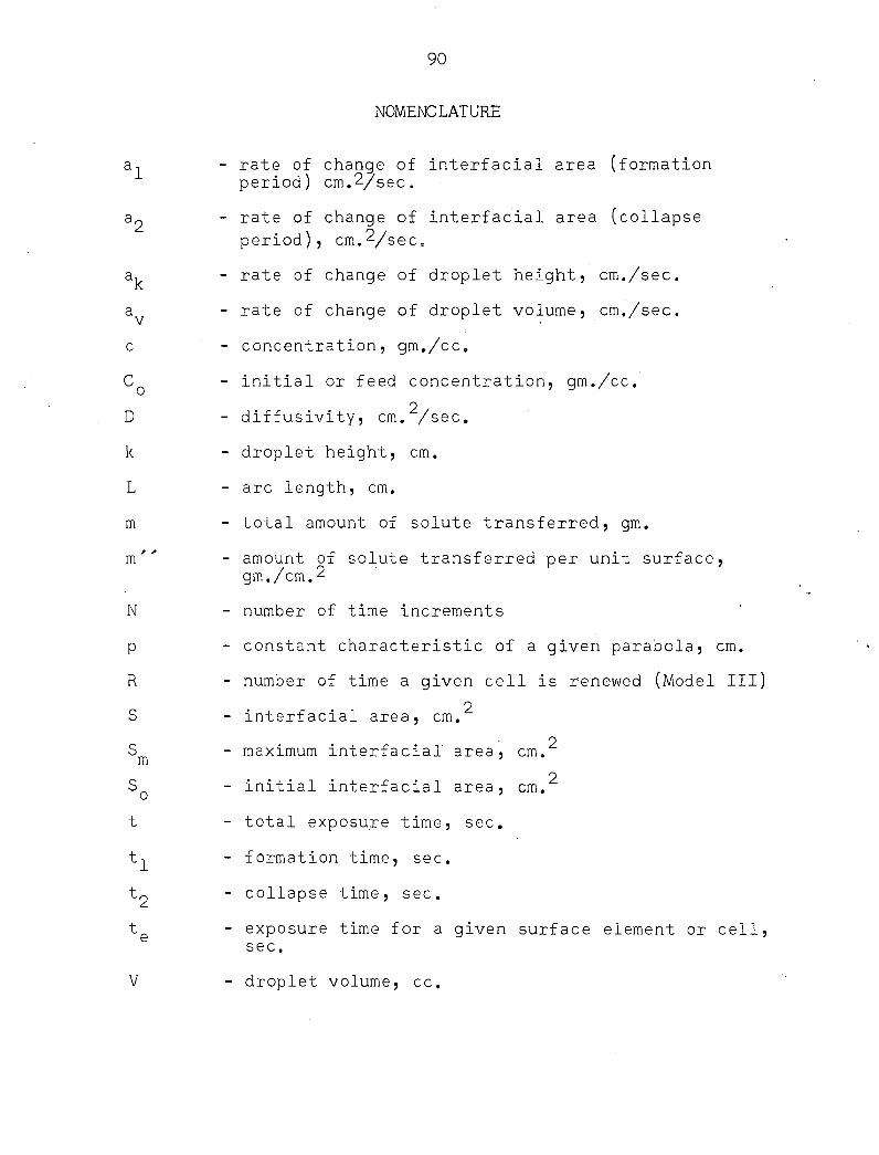
90

NOMENCLATURE

a-, - rate of change of interfacial area (formation period) cm.2/sec.

- rate of change of interfacial area (collapse

period), cm.^/sec.

a, - rate of change of droplet height, cm./sec.

a - rate of change of droplet volume, cm./sec.

c - concentration, gm./cc.

C - initial or feed concentration, gm./cc,

p D - diffusivity, cm. /sec.

k - droplet height, cm.

L - arc length, cm.

m - total amount of solute transferred, gm.

m" - amount of solute transferred per unit surface, gm./cm.2

N - number of time increments

p - constant characteristic of a given parabola, cm.

R - number of time a given cell is renewed (Model III)

2 S - interfacial area, cm.

p S - maximum interfacial area, cm.

p S - initial interfacial area, cm.

t - total exposure time, sec.

t^ - formation time, sec.

±2 - collapse time, sec.

t - exposure time for a given surface element or cell, sec.

V - droplet volume, cc.

91

Vm - maximum droplet volume, cc.

Vt - tangential velocity, cm./sec.

wv w2 - cell dimensions, cm.

0 - time, sec.

p - density, gm./cc.

0j - defined by Equation (44)

0 ' j - defined by Equation (52)

*J-l - defined by Equation (43)

- average flux, defined by Equation (63), gm./cm.^sec.

92

LITERATURE CITED

1. Beekj W. J. and Kramers, H. Mass transfer with a change in interfacial area. Chem. Engr. Sci. 16: 909-921. 1962.

2. Coulson, J. M. and Skinner, S. J. The mechanism of liquid-liquid extraction across stationary and moving interfaces. Chem. Engr. Sci. 40: 197-211. 1952.

3. Danckwerts, P. V. Significance of liquid-film coeffi­cients in gas absorption. Ind. Engr. Chem. 43: 1460-1467.

4. Davies, J. T. and Rideal, E. K. Interfacial phenomena. New York, N. Y., Academic Press. 1961.

5. Facto, L. A. and Catron, D. V. Time lapse cinematography as a method of studying animal behavior and ration preferences. Journal of the Biological Photographic Association 29: 113-123. 1961.

6. Farmer, W. 5. Controlling variables in liquid-liquid extraction from single drops. (Oak Ridge National Laboratory) U. S. Atomic Energy Commission Report ORNL-635. 1950.

7. Fritz, J. S. Acid-base titrations in nonaqueous solvents. Colûmbus, Ohio, G. Frederick Smith Chemical Co. 01952.

8 Granville, W. A., Smith, P. F., and Longley, W. R. Elements of calculus. New York, N. Y. , Ginn and Co. 1946. Co. 1946

9. Gregory, C. L. Mass transfer between forming drops and a continuous liquid phase. Microfilm copy. Unpublished D.Sc. thesis. Cambridge, Mass., Library, Massachusetts Institute of Technology. 1957.

10. Harriott, P. A random eddy modification of the penetra­tion theory. Chem. Engr. Sci. 17: 149-154.

11. . A review of mass transfer to interfaces. Can. J. Chem. Engr. 40: 60-69.

12. Higbie, R. The rate of absorption of a pure gas into a still liquid during short periods of exposure. Trans. A. I. Ch. E. 35: 365-389. 1935.

93

13. Himmelblauj D. M. and Bischoff , K. B. New developments in mass transfer. Ind. Engr. Chem. 55: 50-57. 1963.

14. Johnson, A. I., Hamielec, A., Ward, D. and Golding, A. End effect corrections in heat and mass transfer studies. Can. J. Chem. Engr. 36: 221-227. 1958.

15. Johnson, W. W. Treatise on integral calculus. New York, N. Y., John Wiley and Sons, Inc. 1907.

16. Kishinevsky, M. K. The theoretical work of Danckwerts in the field of absorption. (Translation) Journal of Applied Chemistry USSR 27: 359-365. Jan.-June 1954.

17. Kronig,.R. and Brink, J. C. On the theory of extraction from falling droplets. App'l. Sci. Res. A2: 142-154. 1949/51.

18. Lewis, J. B. The mechanism of mass transfer of solutes across liquid-liquid interfaces. Part I. The determination of individual transfer coefficients for binary systems. Chem. Engr. Sci. 3: 248-259. 1954.

19. . The mechanism of mass transfer of solutes across liquid-liquid interfaces. Part II. The transfer of organic solutes between solvents and aqueous phases. Chem. Engr. Sci. 3: 260-278. 1954.

20. Licht, W. and Conway, J. B. Mechanism of solute transfer in spray towers. Ind. Engr. Chem. 42: 1152-1157. 1950.

21. and Pansing, W. F. Solute transfer from single drops in liquid-liquid extraction. Ind. Engr. Chem. 45: 1885-1896. 1953.

22. Michels, H. H. The mechanism of mass transfer during bubble formation. Microfilm copy, No. 60-5365. Unpublished Ph.D. thesis, Newark, Delaware, University of Delaware. Ann Arbor, Mich., Univer­sity Microfilms, Inc. 1960.

23. Orell, A. and Westwater, J. W. Spontaneous interfacial cellular convection accompanying mass transfer: Ethylene glycol-acetic acid-ethyl acetate. A. I. Ch. E. J . 8: 350-356. 1962.

24,

25,

26,

27

28

29

30

31

32

33

34

94

Sherwood, T. K. , Evans, J. E. and Longcor, J. V. A. Trans. Am. Inst. Chem. Engrs. 35: 597-662. 1939.

and Wei, J. C. Interfacial phenomena in liquid extraction. Ind. Engr. Chem. 49: 1030-1034. 1957.

Sternling, C. V. and Scriven, L. E. Interfacial turbu­lence: Hydrodynamic instability and the Marangoni effect. A. I. Ch. E. J. 5: 514-523. 1959.

Treybal, R. C. Liquid extraction. Ind. Engr. Chem. 52: 262-266. I960.

Van Nes, K. and Van Westen, H. A. Aspects of the constitu­tion of mineral oils. New York, N. Y., Elsevier Publishing Co. Inc. 1951.

Ward, A. F. H. and Brooks, L. H. Diffusion across inter­faces. Trans. Faraday Soc. 48: 1124-1136. 1952.

West, F. B., Herrman, A. J., Chong, A. T., and Thomas, L. E. Addition agents and interfacial barriers in liquid-liquid extraction. Ind. Engr. Chem. 44: 624-631. 1952.

, Robin, P. A., Moregenthaler, A. C., Jr., Beck, T. R. and McGregor, D. K. Liquid-liquid extraction from single drops. Ind. Engr. Chem. 43: 234-238. 1951.

Whitman, W. F. The two-film theory of gas absorption. Chem. Met. Engr. 29: 146-148. 1923.

Wilke, C. R. and Chang, P. Correlation of diffusion coefficients in dilute solutions. A. I. Ch. E. J. 1: 264-270. 1955.

, Prausnitz,'J. M., and Acrivos, Andreas. Mass transfer. Ind. Engr. Chem. 52: 441-446. 1960.

95

ACKNOWLEDGEMENTS

The author wishes to.express his appreciation and thanks

to Dr. L. E. Burkhart for his guidance and encouragement

during the author's graduate work. Special thanks are due

the author's wife for her patience and especially for her

help in the preparation of this manuscript. Thanks are also

due the research helpers who assisted with various portions

of this investigation.

96

APPENDIX A

Experimental Data

Table 6. Run G-9--feed concentration 9.85 wt. % acid

Exposure Sample % acid Ave. Interfacial Water Time Cone. Rem. Flux,. Condition Flow rate Sec. Wt. % x 10^ cc/min.

12 8.76 88.9 19.5 Ta 310 12 8.71 88.4 20.4 T, 310 16 9.02 91.6 11.4

T, 310

16 8.99 91.3 11.5 ' N 310 16 8.90 90.4 12.7 N 310 16 8.86 90.0 13.3 N 310 20 8 .46 85.9 14.9 T 310 20 8 .50 86.3 14.5 T 310 20 8.53 86.6 14.2 T 310 20 8.52 86.5 14.3 T 310 20 8 .50 86.3 14.5 T 310 22 8 .52 86.5 13.0 T 310 22 8 .83 89.6 10.0 N 310 22 8 .94 90.8 8 .9 N 310 22 8.87 90.1 9 .6 N 310 30 8 .73 88.6 8 .0 T 310 30 8 .70 88.3 8 .2 T 310 30 8.80 89.3 7.5 T 310 40 8.51 86.4 7 .2 T 310 40 8.62 87.5 6.6 T 310 40 8.56 86.9 6 .9 T 310 40 8.70 88.3 6 .2 T .310 40 8.62 87.5 6.6 T 310 50 8.67 88.0 5.1 N > 310. 50 8 .74 88.7 4 .8 N 310 50 8.69 88.2 5.0 „ N 310 50 8 .53 86.6 5.7 N 310 50 8.77 89.0 4.6 N 310 60 8 .04 81.6 6.5 T 310 60 8 .42 85.5 5.1 T 310 60 8.45 85.8 5 .0 T 310

^Denotes interfacial activity was present.

^Denotes interfacial activity was absent.

po; Tir Sec

12 12 12 12 12 12 16 16 16 16 16 20 20 20 22 22 22 22 22 30 30 30 30 30 40 40 40 40 40 50 50 50 50 60 60

97

Run G-10--feed concentration 9.70 wt. % acid

Sample % acid Av. interfacial Water Cone. Rem. Flux Condition Flow rate Wt. % x 10 cc/min.

8.64 89.1 19.0 T 310 8.81 90.8 15.9 T 310 8.85 91.2 15.2 T 310 8.78 90.5 16.4 T 310 8.73 90.0 17.4 T 310 8.82 90.9 15.7 T 310 8.52 87.8 15.8 T 310 8.59 88.6 14.9 T 310 8.50 87.6 16.1 T 310 8.55 88.1 15.4 T 310 8.61 88.8 14.6 T 310 8.54 88.0 12.5 T 310 8.43 88.9 13.6 T 310 8.59 88.6 11.9 T 310 8.53 87.9 11.4 T 310 8.63 89.0 10.4 T 310 8.39 86.5 12.8 T 310 8.55 88.1 11.2 T 310 8.38 86.4' 12.9 T 310 8.52 87.8 8 .4 T 310 8.57 88.4 8.1 T 310 8.51 87.7 8 .5 T 310 8.42 86.8 9 .2 T 310 8.58 88.5 8 .0 T 310 8.32 85.8 7.4 T 310 8.15 84.0 8 .3 T 310 8.36 86.2 7.2 T 310 8.41 86.7 6 .9 T 310 8.26 85.2 7.7 T 310 7.89 81.3 7.8 . T 310 8.09 83.4 6 .9 T 310 8.23 84.9 6 .3 T 310 8.22 84.7 6 .4 T 310 8.12 83.7 5.7 T 310 8.08 83.3 5.8 T 310 8.20 84.5 5.4 T 310 7.99 82.4 6.1 T 310 8.21 84.6 . 5 .3 T 310

po: Tir Se<

12 12 12 12 16 16 16 16 20 20 20 20 30 30 30 30 40 40 40 40 50 50 50 50 50

98

Run G-ll--feed concentration 9.83 wt. % acid

Sample % acid Av. Interfacial "Water Cone. Rem. Flux Condition Flow rate Wt. % x 10^ cc/min.

9.28 94 .4 9 .8 N 9.41 95 .7 7 .5 N 9.41 95 .7 7.5 N 9.31 94 .7 9 .3 N 9.27 94 .3 7 .5 N 9.32 94 .8 6.8 N 9.38 95 .4 6.0 N 9.34 95 .0 6.6 N 8.89 90 .4 10.1 T 8.93 90 .8 9.7 N 9.05 92 .1 8 .4 T 9.00 91 .6 8 .9 T 8.88 90 .3 6.8 N 8.93 90 .8 6 .4 N 9.05 92 .1 5.6 N 9.08 92 .4 5.4 T 8.69 88 .4 6.1 N 8.84 89 .9 5 .3 N 9 .04 92 .0 4 .2 N 8.90 90 .5 5 .0 T 8.81 89 .6 4 .4 N 8.77 89 .2 4 .5 N 8 .65 88.0 5.1 T 8.72 88 .7 4 .8 N 8.74 88 .9 4.7 N

99

Table 9. Run G-3--feed concentration 14.56 wt. % acid

Exposure Sample % acid Av. Interfacial Water Time Cone. Rem. FluXr

x 10^ Condition Flow rate

Sec. Wt. % FluXr x 10^ cc/min.

10 13.67 93 .9 19 .2 95 12 13.61 93 .5 17.1 T 95 12 13.60 93 .4 17.3 T 95 12 13.52 92 .9 18 .7 T 95 12 13.75 94 .4 14 .5 T 95 12 13.62 93 .5 16 .9 T 95 12 13.53 92 .9 18 .5 242 12 13.52 92 .9 18.7 242 12 13.46 92 .5 19 .7 242 12 13.65 93 .8 16 .4 242 12 13.63 93 .6 16.7 242

• 12- 13.61 93 .5 17.1 410 12 13.45 92 .4 19 .9 410 12 13.62 93 .5 16 .9 410

• 16 13.55 93 .1 13 .6 242 16 13.64 93 .7 12 .4 242 16 13 .64 93 .7 12 .4 242 16 12.90 88 .6 22 .3 410 16 12.93 88 .8 22 .0 410 16 13.18 90 .5 18 .6 410 16 13.17 90 .5 18.7 410 20 12.23 84 .0 25 .1 95 20 12 .32 84 .6 24.1 95 20 12 .38 85 .0 23 .5 242 20 12 .42 :85 .3 23 .0 242 20 12 .48 85 .7 22 .4 242 20 12 .02 82 .55 27 .3 445 20 12 .72 87 .4 19 .8 445 20 12 .26 84 .2 24 .8 410 20 12 .26 84 .2 24 .8 410 30 11.78 80.9 18 .8 95 30 11 .92 81 .9 18 .9 95 30 12 .28 84 .3 16 .4 95 30 12 .42 85 .3 15 .3 242 30 12 .70 87 .2 13 .3 242 30 12 .44 85 .4 15.2 242 40 11.78 80.9 14 .9 95 40 12.29 84 .4 12 .2 95 40 12 .20 83 .8 12.7 95 40 12 .60 86 .5 10.5 242 40 12 .45 85 .5 11 .4 242 40 12 .58 8G.4 10.7 410

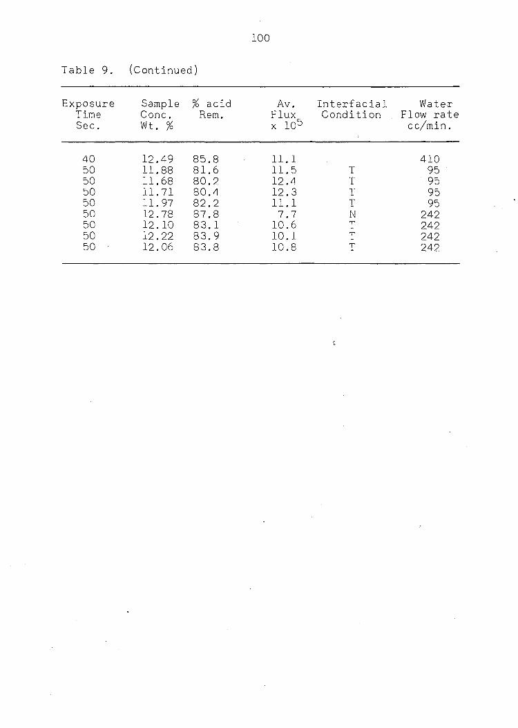
Table 9. (Continued)

100

Exposure Sample % acid Av. Interfacial Water Time Cone. Rem. Flux Condition Flow rate Sec. Wt. % x 105 cc/min.

40 12.49 85 .8 11.1 410 50 11.88 81 .6 11.5 T 95 50 11.68 80 .2 12 .4 T 95 50 11.71 80.4 12 .3 T 95 50 11.97 82.2 11.1 T 95 50 12.78 87 .8 7.7 N 242 50 12 .10 83 .1 10 .6 T 242 50 12.22 83 .9 10.1 T 242 50 12.06 83 .8 10 .8 T 242

po Tii Se,

20 20 20 20 30 30 30 30 30 30 30 30 30 40

101

Run G-12--feed concentration 14.58 wt. % acid

Sample % acid Av. Interfacial "Water Cone. Rem. Flux Condition Flow rate Wt. % x 10^ cc/min.

11.85 81 .3 29 .5 T 12.00 82 .3 27 .8 • T 11.82 81 .1 29 .8 T 11.55 79.2 32 .7 T 11.47 78.7 22 .4 T 11.26 77 .2 23 .9 T 11.83 81.1 19.8 T 11.59 79 .5 21.5 T 11.75 80 .6 20 .4 T 11.99 92 .2 18 .6 T 12.08 82 .9 18 .0 T 12.49 85 .7 15 .0 T 12.45 85 .4 15 .3 T 11.94 81.9 14 .2 T

102

Table 11. Run G-4--feed concentration 19.47 wt. % acid

Exposure Sample % acid Ave. Interfacial Water Time Cone. Rem. Flux Condition Flow rate Sec. Wt. % x 10& cc./min.

30 17 .72 91 .0 12 .7 T 480 30 17.71 91.0 12.7 T 480 40 16.58 85 .2 15 .7 T 135 40 16 .52 84 .9 16 .0 T 135 40 16 .70 85 .8 15 .0 T 135 40 17 .25 88 .6 12 .0 T 310 40 17 .40 89 .4 11.2 T 310 40 17 .40 89 .4 11.2 T 310 40 17 .22 88 .4 12 .2 T 310 40 18 .70 96 .1 4 .2 N 310 40 16.67 85.6 15 .2 T 480 40 17.4 89.1 11.5 T 480 40 17 .59 90 .3 10 .2 T 480 40 17 .35 89 .1 11.5 T 480 50 17 .03 87 .5 10 .6 T 135 50 16 .98 87 .2 10 .8 T 135 50 17 .13 88 .0 10 .2 T 135 50 17 .22 88 .4 9 .8 N 135 50 17.27 88.7 9 .5 N 135 50 17 .51 89 .9 8 .5 N 310 50 17.67 90.8 7 .8 N 310 50 17 .62 90 .5 8 .0 N 310 50 16 .07 82 .5 14 .8 N 480 50 16 .59 85 .2 12.5 N 480 50 16 .44 84 .4 13 .2 N 480 12 16.55 85 .0 52 .6 T 135 12 16.59 85 .2 51.9 T 135 16 16 .61 85 .3 38 .7 T 135 20 16.31 83 .8 34 .3 T 135 20 16 .30 83 .7 34 .4 T 135 20 16.59 85 .2 31-.2 T 310 20 16 .86 86 .6 28 .3 T 310 20 17 .60 90 .4 20 .3 N 310 20 17 .61 90 .5 20 .2 N 310 20 17.14 88.0 25 .3 N 480 20 16 .84 86 .5 28 .5 T 480 20 16 .59 85 .2 31 .2 T 480 20 16 .65 85 .5 30 .6 T 480 22 17 .95 92 .2 15.0 N 480 22 17.76 91 .2 16 .9 N 480

Tii Se

22 22 22 22 22 22 30 30 30 30 30 30

103

(Continued)

Sample % acid Ave. Interfacial Water Cone. Rem. Flux Condition Flow rate Wt. % x 105 cc./min.

18 .22 93 .6 12 .3 N 480 18.15 93.2 13 .0 N 480 17.35 89.1 20 .9 N 310 16 .62 85 .4 28 .1 T 135 16 .46 84 .5 29 .7 T 135 16 .36 . 84 .0 ' 30 .7 T 135 17 .14 88 .0 16 .9 T 135 17 .29 88 .8 15 .8 T 135 17.16 88.1 16 .7 T 135 17.19 88.3 16.5 N 310 16 .99 87 .3 17 .9 N 310 16 .91 86 .9 18 .5 T 310

104

Table 12. Run G-6--feed concentration 19.53 wt. % acid

Exposure Sample % acid Av. Interfacial Water Time Cone. Rem. Flux, Condition Flow rate Sec. Wt. % x 10^ cc/min.

12 18 .04 92 .4 26 .9 N 310 12 18.28 93 .6 22 .6 N 310 12 17.87 91.5 30 .0 N .310 12 17.82 91 .2 30 .9 N 310 12 18.7 95 .7 15 .2 N 497 12 18.77 96 .1 13 .7 N 497 12 18 .75 96 .0 14.1 N 497 14 18.14 92 .9 21 .6 T 310 14 18.59 95 .2 14 .6 N 310 14 18.74 96.0 12 .3 ' N 310 14 18 .64 95 .4 13 .8 N 310 16 17 .64 90 .3 25 .6 T 310 16 17.32 88 .7 30 .0 T 310 16 17.70 90 .6 24 .8 T 310 16 18.02 92 .3 20 .5 N 310 16 17.95 91.9 24 .1 N 310 18 18 .01 92 .2 18 .3 T 310 18 18.33 93 .9 14 .5 T 310 18 18.19 93 .1 16 .2 T 310 50 17 .23 88 .2 10.0 N 310 50 17.17 87.9 10 .2 N 310 60 17 .77 91 .0 6.4 N 310 60 17 .94 91 .9 5 .8 N 310 60 17 .90 91.7 5.9 N 310 60 17.91 91.7 5.9 N 310 60 18 .27 93 .6 4.6 N 497 60 18 .12 92 .7 5 .2 N 497 60 17 .88 91 .6 6.0 N 497 60 17 .90 91 .7 5 .9 N 497

105

Table 13. Run G-7--feed concentration 19.57

Exposure Sample % acid Av. Interfacial Water Time Cone. Rem. Flux Condition Flow rate Sec. Wt. % x 105. cc/min.

10 18 .52 10 18.33 10 17.68 ' 12 18.36 12 18.49 16 18.38 16 18.16 16 18.47 16 18.13 20 17.71 20 17.42 20 18 .04 20 18.11 20 17 .88 22 17.79 22 17 .94 22 18.47

94 .6 22 .8 93 .7 26 .9 90 .3 41 .0 93 .8 21 .9 94 .5 19 .5 93 .9 16.1 92.8 19.1 94.4 14.9 92.6 19 .5 90 .5 20 .2 89 .0 23 .2 92 .2 16.6 92.5 15 .8 91 .4 18 .4 90 .9 17 .6 91.7 16.1 94 .4 10 .8

N 310 N 310 N 310 N 310 N 310 N 310 N 310 N 310 N 310 N 310 N 310 N 310 N 310 T 310 N 310 N 310 N 310

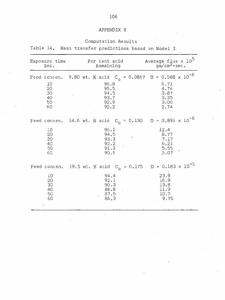
106

APPENDIX B

Computation Results

Table 14. Mass transfer predictions based on Model I

Exposure time Sec.

Per cent acid Remaining

Average flux x 10v gm/cm^-sec.

Feed concen. 9.80 wt. % acid C = 0.0867 D = 0.588 x 10

10 20 30 40 50 60

96.8 95 .5 94 .5 93 .7 92 .9 92 .2

6 .71 4 .74 3 ,87 3 .35 3 .00 2 .74

Feed concen. 14.6 wt. % acid C = 0.130 D.= 0.891 x 10

10 20 30 40 50 60

96 .1 94 .5 93 .3 92 .2 91 .3 90 .5

12 .4 8 .77 7 .17 6 .21 5 .55 5 .07

Feed concen. 19.5 wt. % acid CQ - 0.175 D = 0.183 x 10 ̂

10 94 .4 23 .9 20 92 .1 16 .9 30 90 .3 13 .8 40 88 .8 11 .9 50 87 .5 10 .7 60 86 .3 9 .75

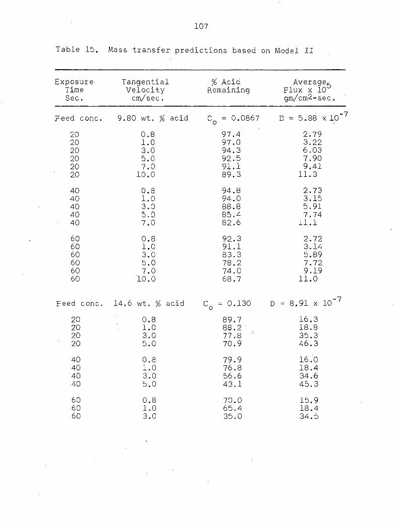
107

Table 15. Mass transfer predictions based on Model II

Exposure Tangential % Acid Average^ Time Velocity Remaining Flux x 10 Sec. cm/sec. gm/cm2-sec.

Feed conc. 9.80 wt. % acid C = 0.0867 D = 5.88 x 10 ̂

20 0 .8 97 .4 2 .79 20 1 .0 97 .0 3 .22 20 3 .0 94 .3 6 .03 20 5 .0 92 .5 7 .90 20 7 .0 91 .1 9 .41 20 10 .0 89 .3 11 .3

40 0 .8 94 .8 2 .73 40 1 .0 94 .0 3 .15 40 3 .0 88 .8 5 .91 40 5 .0 85 .4 7 .74 40 7 .0 82 .6 11 .1

60 0 .8 92 .3 2 .72 60 1 .0 91 .1 3 .14 60 3 .0 83 .3 5 .89 60 5 .0 78 .2 7 .72 60 7 .0 74 .0 9 .19 60 10 .0 68 .7 11 .0

Feed conc. 14.6 wt. % acid C = 0.130 D = 8.91 x 10 ̂

20 0 .8 89 .7 16 .3 20 1 .0 88 .2 18 .8 20 3 .0 77 .8 35 .3 20 5 .0 70 .9 46 .3

40 0 .8 79 .9 16 .0 40 1 .0 76 .8 18 .4 40 3 .0 56 .6 34 .6 40 5 .0 43 .1 45 .3

60 0 .8 70 .0 15 .9 60 1 .0 65 .4 18 .4 60 3 .0 35 .0 34 .5

108

Table 15. (Continued)

Exposure Time Sec.

Tangential Velocity cm/sec.

% Acid Remaining

Average Flux x 10 gm/cm^-sec

Feed conc. 19.5 wt. % acid Cg = 0 .175 D - 1.83 x 10

20 0 .8 95 .4 9 .95 20 1.0 94.6 11 .5 20 3 .0 90 .0 21 .5 20 5 .0 86 .8 28 .2 20 7.0 84.3 33 .5 20 10 .0 . 81 .2 40 .3

40 0.8 90 .9 9 .73 40 1.0 89.5 11.2 40 3.0 80 .3 21 .0 40 5.0 74 .2 27 .6 40 7.0 69.3 32 .8 40 10 .0 63 .1 39 .4

60 0 .8 86 .4 9 .70 60 1.0 84.3 11.2 60 3 .0 70 .6 21 .0 60 5 .0 61 .4 27 .5 60 7.0 54.0 32 .8 60 10.0 44.8 39 .3

109

Table 16. Mass transfer predictions based on Model III

Exposure Cellular % Acid Average ^ Time Exp. Time Remaining f lux X 10̂ Sec. Sec. gm./cm.2-sei

Feed conc. 9.80 wt. % acid C^ = 0 .0867 D = 5 .88 x 10

20 0 .06 70 .9 30 .8 20 0 .08 74 .8 26 .7 20 0.10 77.5 23.9 20 0 .20 84.1 16.9 20 0 .40 88 .7 11.9 20 0 .60 90 .8 9 .74 20 0 .80 92 .0 8 .43 20 1.00 92.9 7 .54 20 1 .20 93 .5 6 .89 20 1.40 94.0 6 .38 20 1 .60 94 .4 5 .96

40 0.06 42 .2 30 .6 40 0.08 50 .0 26 .5 40 0.10 55.3 23 .7 40 0 .20 68 .4 16 .8 40 0 .40 77.6 11.9 40 0 .60 81.7 9.68 40 0.80 84 .2 8 .38 40 1 .00 85 .8 7 .50 40 1.20 87 .1 6 .84 40 1.40 88.0 6 .34 40 1 .60 88 .8 ' 5 .93

60 0 .06 13.4 30.6 60 0 .08 25 .0 26 .5 60 0 .10 32 .9 23 .7 60 0 .20 52 .6 16.7 60 0 .40 66 .5 11.8 60 0 .60 72 .6 9 .67 60 0 .80 76 .3 8 .37 60 1 .00 78 .8 7 .49 60 1 .20 80 .6 6 .84 60 1.40 82.1 6 .33 60 1 .60 83 .2 5 .92

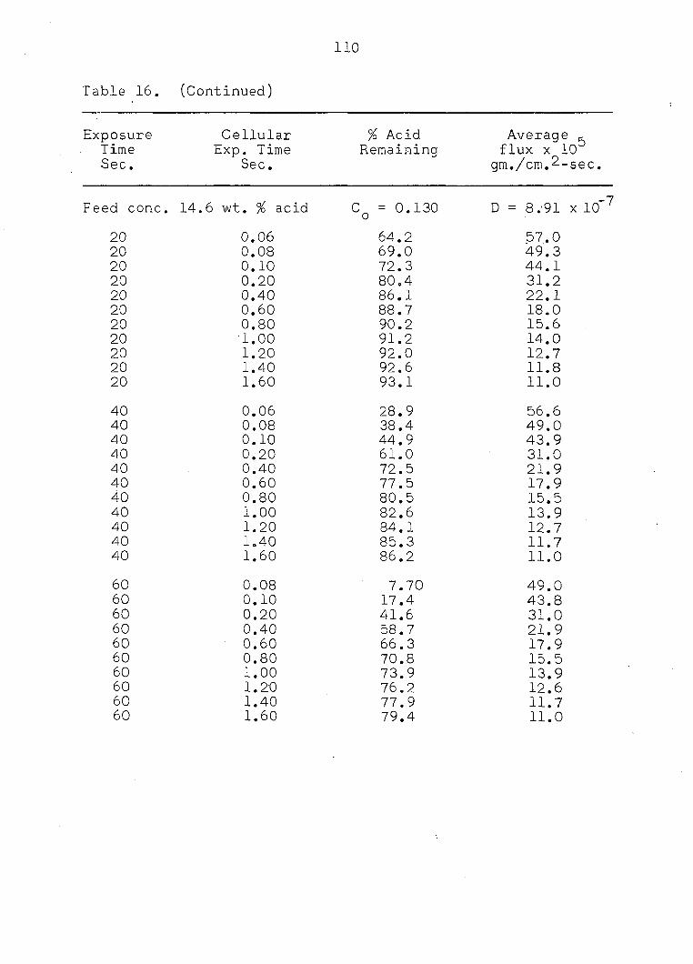
110

Table 16. (Continued)

Exposure Time Sec.

Cellular Exp. Time

Sec.

% Acid Remaining

Average ^ flux x 10 gm./cm.2-sec,

Feed conc. 14.6 wt. % acid C = 0.130 D = 8.'91 x 10 ̂

20 0 .06 64 .2 57 .0 20 0 .08 69 .0 49 .3 20 0 .10 72 .3 44.1 20 0.20 80 .4 31 .2 20 0 .40 86 .1 22 .1 20 0 .60 88 .7 18 .0 20 0 .80 90 .2 15 .6 20 1 .00 91 .2 14 .0 20 1 .20 92 .0 12.7 20 1.40 92.6 11.8 20 1 .60 93 .1 11.0

40 0 .06 28 .9 56.6 40 0.08 38 .4 49 .0 40 0.10 44 .9 43 .9 40 0.20 61 .0 31 .0 40 0 .40 72 .5 21 .9 40 0 .60 77 .5 17.9 40 0.80 80 .5 15 .5 40 1 .00 82 .6 13 .9 40 1 .20 84 .1 12 .7 40 1.40 85.3 11 .7 40 1.60 86 .2 11.0

60 0 .08 7.70 49.0 60 0 .10 17.4 43.8 60 0 .20 41 .6 31 .0 60 0 .40 58 .7 21 .9 60 0 .60 66.3 17.9 60 0 .80 70 .8 15.5 60 1 .00 73 .9 13 .9 60 1 .20 76 .2 12 .6 60 1 .40 77 .9 11.7 60 1 .60 79.4 11.0

Ill

Table 16. (Continued)

Exposure Time Sec.

Cellular Exp. Time

Sec.

% Acid Remaining

Average flux x 10 gm./cm.2-sec.

Feed conc. 19.5 wt. % acid C^ = 0 .175 D = 1 .83 x 10"^

20 0 .06 48 .7 110 .0 20 0 .08 55 .6 95 .0 20 0 .10 60 .3 84 .9 20 '0 .20 71 .9 60 .1 20 0 .40 80 .1 42 .5 20 0 .60 83 .8 34.7 20 0 .80 86 .0 30 .0 20 1 .00 87 .4 26 .9 20 1 .20 88 .5 24 .5 20 1 .40 89 .4 22 .7 20 1 .60 90 .1 21 .2

40 0.08 11.7 94.4 40 0.10 21.1 84.4 40 0.20 44 .2 59 .7 40 0.40 60 .5 42 .2 40 0 .60 67 .8 34 .5 40 0 .80 72 .1 29 .8 40 1.00 75 .0 26 .7 40 1.20 77 .2 24 .4 40 1 .40 78 .9 22 .6 40 1 .60 80 .3 21.1

60 0 .20 16 .3 ' 59 .6 60 0 .40 40 .8 42 .2 60 0 .60 51 .7 34 .4 60 0 .80 58 .2 29 .8 60 1 .00 62 .6 26 .7 60 1 .20 65 .8 24 .3 60 1 .40 68 .4 22 .5 60 1 .60 70.4 21.1

112

Digital Computor Programs

Table 17. Nomenclature for Model I

o

o O

S - SO 0 Vm " DPVOL

D - D t - TEX P " RHO

Sm - SM t]_ - T1 Tj) - FLUX

Table 18. Nomenclature for Model II

• ak - Ak m(t ) - TOATR yn - Y1

AV Pn - PI vt - VT

Co.- CO Pn+1 - P2 yn+l - Y2

D - D (Slav - AAVG(MO) zn - ZI

km - GKMAX <Sj >0n

- Al(MO) zn+l - Z2

kn - ZK1 (Sj'en+1 - A2(MO) A© - DELT

kn+l ZK2 So - SO ASj - DELAR

(Lj'av - HLAVG(MO) t - TEXTOT - CON

( V e n * ALI . . (te}j - TEX(MOX) - CONLT

'Lj'en+1' - AL2 Vn - VI Azn

- DELZ1

( m j ) - GM Vn+1 - V2 - DE-LZ2

(m:) - GMLTE Vm - VMAX 4» - FLUX

113

Table 19. Nomenclature for Model III

ak - AK (mVn

- GM(NO) Vm " VMAX

- AV Pn - PI Vn " VI

D • - D Pn+1 - P2 ' Vn+1 " V2

Co - CO R - CON Vt - VT

km - GKMAX Sav - SAVG - Q1

kn - ZK1 Sn

- SI w2 - Q2

kn+l - ZK2 Sn+1 - S2 *9n " DELT

m(t ) - TOATE te - TEX i> ~ FLUX

Table 20. Input data for computor calculations

Sm = 1.81 cm. ̂ "So = 0. 725.cm.^ Vm = 0-31 cc.

Feed concentration wt. % acid

Co gm./cc.

D p

cm. /sec. P

gm./cc.

9.8 0.0887 5.88x10"? 0.8874

14.6 0.1303 8.91x10"? 0.8922

19.8 0.1750 1.33x10"^ 0.8974

114

READ 201, SM, SO, DPVOL, N 201 FORMAT (3612.4,12) 202 READ 203, C, 0, RHO, K 203 FORMAT (3E12.4.I2)

PRINT 204 204 FORMAT (29H1GOLOEN MOL DIFFUSION MODEL I)

PRINT 205,RHO, C, D 205 FORMAT 15HJRH0=E12.4,3H C = E12.4,3H D=E12.4)

PRINT 206 206 FORMAT (87HJ TEX GTFOR

IT PCREM FLUX ) 00 500 J=1,N,1 XJ-J Tl-XJ A=(SM-SO)/T1 B=SORTF(T1) Q=2.0»S0»B R=t4.0»A»B»Tl)/3.0 E=t2.0»C)«ISQRTF(DZ3.1416)) GTFOR=E*10*R) H=2.0»SM»B GTCOL = E5 î M-R) TOT AD=DPVOL»C PCEXT=((GTCOL+GTFOR)•(100.0))/TOTAO PCREM*100.00-PCEXT FLUX=CGTFOR>GTCOL)/((2.0»T1)•1SO+SM)/2.0) TEX=2.0*T1 PRINT 207,TEX,GTFOR,GTCOL.PCEXT,PCREM,FLUX

207 FORMAT 1F7.1,2E20.8,2F10.4,E20.8) 500 CONTINUE

IF (K) 600,600,202 600 STOP 89

END

002 003 004 005 006 007 008 009 010

GTCOL PCEX Oil 0 1 2 013 014 015 016 017 018 019 020 021 022 023 024 025 026 027 028 029 030 031 032 033 034

Figure 21. Full Fortran statements, Model I

115

READ 333,50 JOG 333 FORMAT (E15.8) JOG

READ 200, VMAX.GKMAX JOG 03 2 200 FORMAT (2E12.4) JOG 003

READ 201, TEX I,TE IN, TEMAX JOG 304 201 FORMAT (3E12.4) JOG 005 281 READ 202,VT,CO,OELT,D,MMAX,LAP JOG 006 202 FORMAT (4E12.4.2I6) JOG 007

READ 282,K1,K2,K3,K4,K5,K6 JOG 00 7 282 FORMAT (613) JOG 007

PRINT 203 JOG 008 203 FORMAT (32H1GOLOEN MODEL II SURFACE RENEWAL ) JOG 009

PRINT 204, VT » CO,0,GKMAX,VMAX.DELT,MMAX JOG 010 204 FORMAT I4HJVT=E11.4,3X3HC0=fc11.4,3X2HD=E11.4,3X6HGKMAX=E11 .4 , 3X5HVJOG Oil

1MAX=E11.4,3X5HDELT=E11.4,3X5HMMAX=I3) JOG 012 DIMENSION TOATR(201 ) JOG DIMENSION T(201),Z1(201),Z2(201),Y1(201),Y2(201), A1(201 ), A21201),JOG 013 1AAVG(201),ALU 201),AL2(201),HLAVG(201),TEX(201) , TEXINI201) ,TOAZI(2J0G 014 201) JOG COMMON T,Z1,Z2,Y1,Y2,A1,A2,AAVG,AL1,AL2.HLAVG.TEX, TEXIN.TOAZI JOG 015 TEXTOT=TEXI JOG 016 IF (K6) 702,702,703 JUG 024

702 PRINT 704 JOG 024 704 FORMAT (85HJ TEXTOT TOATE PCEXT JOG 024

1 PCREM FLUX ) JOG 024 703 CONTINUE JOG 024 280 AK=(GKMAX)•(2.0)/(TEXTOT) JOG 017

AV=(VMAX»2.0)/(TEXTOT) JOG 018 80X=(TEXT0T)/(0ELT) • JOG 019 NMAX=BOX«-l.O JOG 020 DO 210 N=1,NMAX,1 JOG 021 XN=(N-1) JOG 022

210 TIN)=0ELT»XN JOG 023 NIKE-BOX JOG 224 DO 831 N0=1,NIKE, 1 JOG 024 IF (NO—I) 211,211,530 JOG 025

211 T(N0)=T(N0+1) JOG 026 530 IF(NIKE-NO) 531,531,641 JOG 027 531 T î 11 = T(NO) JOG 027 641 CONTINUE JOG 029

•IF ( NO—( NMAX/2 ) ) 212,212,213 JOG 030 212 £K1«AK»T( NO ) JOG 031

V:=AV»T(NO) JOG 032 ZK2=tAK)»T(ND*1) JOG 033 V2=(AV)» T fN0+1 ) JOG 034 GO TO 214 JOG 035

213 ZK1=GKMAX-(T(NO)-<TEXTQT/2.0) )*AK JOG 036 Vl=VMAX-(T(N0)-(TEXT0T/2.0l)»AV JOG 037 ZK2=GKMAX-(T(N0>1)-1TEXTOT/2.0))*AK JOG 038 V2=VMAX-(T(NO*l)-(TEXTOT/2.0 ))»AV JOG 039

214 P1=V1/13.1416»ZK1«ZK1) JOG 040 P2=V2/(3.1416»ZK2»ZK2) JOG 041 J=MMAX-1 JOG 042 XJ=J JOG 043 DELZl=ZK1/XJ JOG 044 DELZ2=ZK2/XJ JOG 045 NP1=N0*1 ' JOG 246 IF (Kl) 235,235,337 JOG 046

235 PRINT 307, TEXTOT,T(NO),ZK1,VI,PI,NO JOG 047 307 FORMAT (8HJTEXTUT=E13.6,3X2HT=E13.6,3X4HZK1=E13.6 ,3X3HV1=E13.6,3X3J0G 04 8

1HP1=E13.6,3X3HN0=I3) JOG 049 PRINT 308, TlNO+l),ZK2,V2,P2,NPl JOG 050

Figure 22. Full Fortran statements, Model II

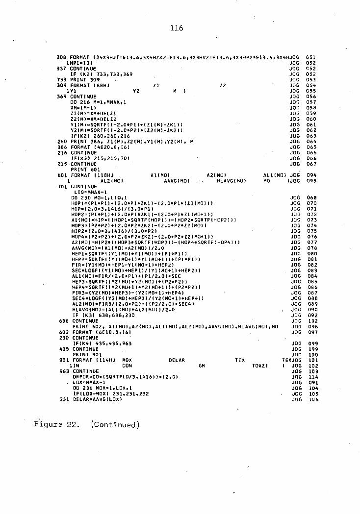
116

308 FORMAT (24X3HJT=E13.6, 3X4HZK2=E13.6, 3X3HV2=E13.6,3X3HP2»E13.6,3X4HJ0G 051 1NP1«I3) JOG 052

337 CONTINUE JOG 052 IF (K2) 733,733,369 JOG 052

733 PRINT 309 JOG 053 309 FORMAT (88HJ ZI 12 JOG 054

1Y1 Y2 M ) JOG 055 369 CONTINUE JOG 056

DO 216 M=1,MMAX,1 JOG 057 XM=(M-1) JOG 058 Z1(M)=XM»DELZ1 JOG 059 Z2(M)=XM«DELZ2 JOG 060 Y1(MI = S0RTF1(-2.0*P1)• ( ZI ( M) -ZK1)) JOG 061 Y2(MI = SQRTF(I-2.C»P21 •(Z2(M1 -ZK2I) JOG 062 IF(K2) 260,260,216 JOG 063

260 PRINT 386, Z1(M),Z2(M) ,Y1(M) ,Y2(M), M JOG 064 386 FORMAT (4E20.8,16) JOG 065 216 CONTINUE JOG 066

IF(K3) 215,215,701 JOG 066 215 CONTINUE JOG 067

PRINT 601 601 FORMAT (118HJ . Al(MO) A21MU) AL1IM0) JOG 094

1 AL21M0) AAVGtMO) HLAVG(MO) MO ) JOG 095 701 CONTINUE

LIQ=MMAX-1 DO 230 M0=1,LIQ,1 JOG 068 H0P1=(P1*PI)+(2.0»P1»ZK1)-(2.0»P1*(ZI(MO) ) ) JOG 070 HIP=(2.0*3.1416)/(3.0»P1) JOG 071 H0P2=(PI»P1)+(2.0»P1*ZK1)-(2.0»Pl*Zl(MO+l)) JUG 072 A1(M0»*HIP*((H0P1»SQRTF (HOP 1))-(H0P2»SQRTF(H0P2))) JUG 073 H0P3=(P2*P2)+(2.0*P2»ZK2)-(2.0*P2*Z2(MO)) JOG 074 HIP2=(2.0*3.1416)/(3.0»P2) JOG 075 H0P4=(P2*P2)+(2.0»P2»ZK2)-(2.0«P2*Z2(MO+l)) JOG 076 A2(MO)=HIP2*((HOP 3*SORTF(H0P3))-(H0P4«SQRTF(H0P4))) JOG 077 AAVG(MO>=(A1(MO)+A2(MO)1/2.0 JOG 078 HEP1 = SQRTFI(Y1(MO)»Y1(MO))+(Pl»Pl)) JOG 080 HEP2=SQRTF((Y1(MO+l)*Y1(MO+l))+(PI*P11) JOG 081 FIR=(Y1(M0)»HEP1-Y1(M0+1)»HEP2) JOG 082 SEC=LOGF((Yl(MO)+HEPl)/(Y1(MO+l)+HEP2)) JOG 083 AL1(MO)=FIR/(2.0»P1)+(P1/2.0)»SEC JOG 084 HEP3=SQRTF(1Y2(MO)»Y2(MO))+(P2*P2)) JOG 08 5 HEP4=SQRTF((Y2(MO+l)*Y2(MO+l))+(P2»P2)) JOG 086 FIR3=lY2(M0)*HEP3)-(Y2(M0+1)*HEP4) JOG 087 SEC4=t0GF((Y2(M0)+HEP3)/(Y2(MO+l1+HEP4)) JOG 08 8 AL2(M01=FIR3/(2.0»P2)+((P2/2.0)•SEC4) JOG 089 HLAVG(M0)=(AL1(M0)+AL2(M0)1/2.0 JOG 090 IF (K31 638,638,230 JOG 09 2

638 CONTINUE JOG 192 PRINT 602, A1(M01,A2(M01,AL1(MO),AL2(MO),AAVG(MO 1,HLAVG(MO 1,MÙ JOG 096

602 FORMAT (6E18.8,16) JOG 097 230 CONTINUE

IF(K4) 435,435,963 JOG 099 435 CONTINUE JOG 199

PRINT 901 JOG 100 901 FORMAT (114HJ MOX DELAR TEX TEXJOG 101

UN CON GM TOAZI 1 JOG 102 963 CONTINUE JOG 103

DRF0R=C0»(S0RTF(D/3.1416))•(2.0) JOG 114 L0X=MMAX-1 JOG 091 DO 236 M0X=1,LOX,1 JOG 104 IFILOX-MOX) 231,231,232 JOG 105

231 DELAR»AAVG(LOX) JOG 106

Figure 22. (Continued)

117

GO TO 233 JOG 107 232 OELAR=(AAVGIMOX)-AAVG(MOX+1 )) JOG 108 233 SUMaO.O JOG 109

DO 234 KIP=1,M0X,1 JOG 110 234 SUM«SUM>HLAVG(KIP) JOG 111

TEX(MOX)=SUM/VT JOG 112 TEXINtMOX)=HLAVG(MOX)/VT JOG 113 CON«(OELT-TEXtMOX))VTEXIN(MOX) JOG 115 GM=ORFOR • (SORTFI TEXIMOX m * IDELAR*CON) JOG 116 CONLT=TEX(MOX)/TEXINIMOX) JOG 117 GMLTE=(DRFOR/2.0)»(SQRTFI TEX IMOX)))*(DELAR*CONLT) JOG 118 TOAZI(MOX)=GM+GMLTE JOG 119 IF (CON) 706,706,711

706 PRINT 707 707 FORMAT 1114HJ MOX OELAR TEX • TEXJOG 101

UN CON GM TOAZI ) JOG 102 708 PRINT 709,MOX,OELAR,TEX(MOX),TEXINIMOX),CON,GM,TOAZI(MOX) 709 FORMAT (1X16,6E18.7) 711 IF ICON» 265,265,712 712 CONTINUE

IF(K4) 943,943,236 JOG 120 943 PRINT 902,MOX,DELAR,TEX(MOX).TEXINIMOX),CON,GM,TOAZI(MOX) JOG 121 902 FORMAT I1X16,6E18.7) JOG 122 236 CONTINUE JOG 123

S=0.0 JOG 125 00 600 K0=1,L0X,1 JOG 126

600 S=S*TOAZIIKO) JOG 127 TOATR(NO)=S JOG 128 IFIK5) 916,916,831 JOG 129

916 CONTINUE JOG 229 237 PRINT 829, TOATRINO), NO JOG 130 829 FORMAT (7HJT0ATR=E16.8,6X3HN0=I4) JOG 131 831 CONTINUE JOG 132

S0T=0.0 JOG 134 LUM=NMAX-1 JOG 135 DO 700 LIP=1« LUM,1 JOG 136

700 SOT»SOT*TOATRI LIP) JOG 137 TOATE=SOT JOG 138 TOTAD=VMAX*CO JOG 139 PCEXT=TOATE*100.CO/TOTAO JOG 140 PCREM=100.00-PCEXT JOG 141 PMAX*VMAX/(3.1416*GKMAX*GKMAX) JOG 402 W=(2.0*3.1416)/(3.0*PMAX) JOG 403 Wl=(PMAX*PMAX+2.0*PMAX*GKMAX) JOG 404 SM=W»((W1)*SQRTF(W1)-(PMAX*PMAX*PMAX)) JOG 405 FLUX=(TOATE*2.0)/l(SO+SM)*(TEXTOT)) JOG 142 IF (K5) 705,705,720 JOG 142

705 PRINT 931 JOG 142 931 FORMAT (85HJ TEXTOT TOATE PCEXT JOG 143

I PCREM FLUX ) JOG 144 720 CONTINUE JOG 144

PRINT 932,TEXTOT, TOATE,PCEXT,PCREM,FLUX JOG 145 932 FORMAT (2XF7.1,E23.8,2F19.2, E23.8) JOG 146

HAWK=TEXTOT-TEMAX JOG 147 IF(HAMK) 261,262,262 JOG 148

261 CONTINUE JOG 248 TEXTOT*TEXTOT+TEIN JOG 149 GO TO 280 JOG 150

262 CONTINUE JOG 151 263 IF (LAP) 265,265,264 JOG 152 264 GO TO 281 JOG 153 265 STOP 89 JOG 154

ure 22. (Continued)

118

READ 200. VMAX,GKMAX,SO JOG 001 200 FORMAT (3E12.4) JOG 002

READ 201, TEX1,TEIN,TEMAX JOG 003 201 FORMAT (3E12.4) JOG 004 400 READ 202, VT,CO,CELT,0,01,02,LAP JOG 005 202 FORMAT (6612.4,13) JOG 006

READ 203, K1,K2 JOG 007 203 FORMAT (213) JOG 008

PRINT 204 JOG 009 204 FORMAT (18H1G0L0EN MODEL III I JOG 010

PRINT 205, VT,CO,OELT.D,GKMAX,VMAX JOG Oil 205 FORMAT (2X4HJVT=E12.4,3X3HCO»E12.4,3X5HDELT= E12.4, 3X2HD-E12. 4.3X6HJ0G 012

1GKMAX3El 2.4,3X5HVMAX=E12.4) JOG 013 206 DIMENSION GM(500),T(500) JOG 014

COMMON GM ,T JOG 015 TEXTOWEXI IFIK1) 207,207,320 JOG 016

207 PRINT 208 JOG 017 208 FORMAT I85HJ TEXTOT TOATE PCEXT JOG 018

1 PCREM FLUX ) JOG 019 320 CONTINUE JOG 020

TEX=(01/VT> JOG 022 CON=1DELT/TEX) JOG 021 TOP = SQRTF(TEX)

209 AK=(GKMAX)»(2.0)/(TEXTOT) JOG 023 AV=(VMAX*2.0)/ITEXT0T) JOG 024 BOX=(TEXTOT)/(DELT) JOG 025 NMAX=1 B0X/2.0)+ 1.0 JOG 026 DO 210 N=1,NMAX,1 JOG 027 XN=(N-1) JOG 028

210 TIN)=DELT»XN JOG 029 NIKE=30X/2.0 JOG 030 DRFOR=(2.0*C0)*ISQRTF(D/3.1416)) JOG 031 IF (K2) 303,303,306 JOG 032

303 PRINT 304, CON,TEX,ORFOR JOG 033 304 FORMAT (2X5HJC0N=E12.5,6X4HTEX=E12.5,6X6HDRF0R=E12 .4) JOG 034 306 CONTINUE JOG

IFIK2) 300,302,302 JOG 035 300 PRINT 301 JOG 036 301 FORMAT 12X116HJ NO GM SAVG SI JOG 037

1 S2 ZK1 VI PI ) JOG 038 302 CONTINUE JOG

DO 224 N0=1,NIKE,1 JOG 039 IFINO-1) 211,211,212 JOG 040

211 TI NO)=T(NO+1) JOG 041 212 CONTINUE JOG 042 213 ZK1=AK*T(N0) JOG 04 3

V1=AV*TINO) JOG 044 ZK2=(AK)*T(NO+l) JOG 045 V2=( AV)»TINOm JOG 046

214 PI=V1/(3.1416»ZK1»ZK1) JOG 048 P2=V2/(3.1416*ZK2*ZK2) JOG 049

215 B1=(P1*P1+2.0*P1*ZK1) JOG 050 216 B2*IP2»P2+2.0*P2*ZK2) JOG 051 218 B3=((2.0*3.1416)/13.0*P1)> JOG 052

B4M(2.0*3.1416)/(3.0*P2>) JOG 053 219 Sl=tB3)»lIB1»SQRTFIB1))-(Pl*Pl»Pl)) JOG 054

S2=(B4)»(IB2*SQRTFIB2))-IP2*P2»P2)) JOG 055 220 SAVG=ISl*S2)/2.0 JOG 056

GNOC=(SAVG)/(Q1*Q2) JOG 057 221 GM(NO)=DRFOR*T0P*01»02*CON*GNOC*2.0 JOG 058

IF (K2) 222,222,224 JOG 059

Figure 23. Full Fortran statements. Model III

119

222 CONTINUE JOG 060 PRINT 223, NO.GM(NO),SAVG,S1,S2,ZK1,V1,P1 JOG 061

223 FORMAT (I6.7E16.5) JOG 062 224 CONTINUE JOG 063

SUM=0.0 JOG 065 DO 225 J=1,NIKE,1 JOG 066

225 SUM=SUM+GM(J) JOG 067 TOATE=SUM JOG 068 TOTAD*VMAX«CO JOG 069 PCEXT=TOATE«100.CO/TOTAD JOG 070 PCREM=100.00-PCEXT JOG 071 PMAX=VMAX/(3.1416»GKMAX»GKMAX) JOG 073 H=C2.0*3.14161/(3.0»PMAX) JOG 074 W1»(PMAX»PMAX+2.0»PMAX»GKMAX) JOG 075 SM-H»(IW1»S0RTF(W1))-(PMAX»PMAX«PMAXI) JOG 076 FLUX=(TOATE* 2.0)/((SO+SM)»(TEXTOT)) JOG 077 IFIK2) 230,230,234 JOG 078

230 PRINT 231 JOG 079 231 FORMAT (85HJ TEXTOT TOATE PCEXT JOG 080

1 PCREM FLUX 1 JOG 081 234 CONTINUE JOG

PRINT 236,TEXTOT,TOATE,PCEXT,PCREM,FLUX JOG 082 236 FORMAT (2XF7. 1 ,E23.8 ,2F19.2,E23.8) JOG 083

HAWK=TEXTOT-TEMAX JOG 084 IF(HAWK) 240,240,242 JOG 085

240 CONTINUE JOG 086 TEXTOT-TEXTOT+TEIN JOG 087 GO TO 320 JOG 088

242 CONTINUE JOG 089 243 IF (LAP) 244,244,246 JOG 090 244 GO TO 400 JOG 091 246 STOP 89 JOG 092

END JOG 093

Figure 23. (Continued)

a

120

APPENDIX C

System Data

Table 21. Viscosity of mineral oil-propionic acid solutions

Temp. = 25°C

Wt. % Acid Viscosity cp

0.00 90 .0

5 .75 62 .0

11 .4 46 .0

16 .7 28 .0

aData taken with a Brookfield Synchro-Lectric Viscometer,

Table 22. Density of mineral oil-propionic acid solutions

Temp. = 21.4°C

Wt. % Acid Density gm./cm. 3

0.00 0 .8686

4 .90 0 .8722

9 .79 0 .8774

14 .9 0 .8827

19 .5 0 .8862

24 .4 0 .8927

121

Table 23. Solute distribution data for the mineral oil-propionic acid-water system

Organic Phase Analysis Aqueous Phase Analysis Wt. % Acid ' Wt. % Acid

0.174 4 .62

0 .409 8 .22

0 .457 9 .02

0 .651 11 .0

0 .780 12 .6

0 .812 13 .0

0 .944 14 .2

1 .13 16 .0

1 .35 18 .3

1 .46 19 .3

1 .75 22 .6 1 .76 22 .8

1 .91 24 .4

2 .18 27 .6

122

APPENDIX D

Derivation of Equation (31)

The differential arc length, dL, of the parabola given

in Figure 6 is

dL.= [1 + (y l )2fAiz (63)

where

y1 = dy/dz (64)

But •

Therefore.

y2 = -2p(z-k) (65)

= -p/y (66)

The surface area determined by revolving the arc length

between z. and z . .about the z axis is J J+1

S = 2tt Z3+l

"ydL (67)

Z j

- 27T J+1y[l+(y1)2]1/2dz (68)

Zj

Substituting Equations (65) and (66) into (68) and integrating

yields

S = §%[(p2+2pk_2pZj)3/2 - (p2+2pk-2pZj+^)3/2], (31)

123

Derivation of Equation (34)

The arc length, L, between z. and zj+]_ in the first

quadrant of Figure 7 may be determined by integrating Equation

(63) between y^ and

dL = [1 + (yl)2]l/2dz (63)

L =

yj+l

[1 + (yl)2]l/2jz

Yn

Again,

= p/y (&&)

and

dz = -y/p dy (70)

Substituting Equations (66) and (70) into (69) yields

l =j 1[i + (p2/y2)]1/2(-y/p)dy (71)

y . J

' j

Equation (34) is obtained upon performing the indicated

integration.

L = è[yj(yj+p2)1/2 " yj+i(yj+i+p2)1/2

, | [ln(yi + (yfP2)1/2 ,j (34) yj+i+(yj+1+p )