Familial collapsing glomerulopathy: Clinical, pathological and immunogenetic features
arX
iv:a
stro
-ph/
0503
459v
1 2
1 M
ar 2
005
Draft version January 17, 2014
Preprint typeset using LATEX style emulateapj v. 11/12/01
B335: A LABORATORY FOR ASTROCHEMISTRY IN A COLLAPSING CLOUD
Neal J. Evans IIDepartment of Astronomy, The University of Texas at Austin, 1 University Station C1400, Austin, Texas
78712-0259, [email protected]
Jeong-Eun LeeDepartment of Astronomy, The University of Texas at Austin, 1 University Station C1400, Austin, Texas
78712-0259, [email protected]
Jonathan M. C. RawlingsDepartment of Physics and Astronomy, University College London, Gower Street, London WC1E 6BT, UK
Minho ChoiTaeduk Radio Astronomy Observatory, Korea Astronomy Observatory, Hwaam 61-1, Yuseong, Daejeon
305-348, [email protected]
Draft version January 17, 2014
ABSTRACT
We present observations of 25 transitions of 17 isotopologues of 9 molecules toward B335. With agoal of constraining chemical models of collapsing clouds, we compare our observations, along with datafrom the literature, to models of chemical abundances. The observed lines are simulated with a MonteCarlo code, which uses various physical models of density and velocity as a function of radius. The dusttemperature as a function of radius is calculated self-consistently by a radiative transfer code. The gastemperature is then calculated at each radius, including gas-dust collisions, cosmic rays, photoelectricheating, and molecular cooling. The results provide the input to the Monte Carlo code. We considerboth ad hoc step function models for chemical abundances and abundances taken from a self-consistentmodeling of the evolution of a star-forming core. The step function models can match the observed linesreasonably well, but they require very unlikely combinations of radial variations in chemical abundances.Among the self-consistent chemical models, the observed lines are matched best by models with somewhatenhanced cosmic-ray ionization rates and sulfur abundances. We discuss briefly the steps needed to closethe loop on the modeling of dust and gas, including off-center spectra of molecular lines.
Subject headings: ISM: abundances — ISM: molecules — ISM: individual (B335) — astrochemistry
1. introduction
The Bok globule, B335, is a rather round dark globuleat a distance of about 250 pc (Tomita et al. 1979). Itis perhaps the best case for being a collapsing protostar.Observations of CS and H2CO lines (Zhou et al. 1993;Choi et al. 1995) were reproduced very well with mod-els of inside-out collapse (Shu 1977). To the extent thatsuch models may describe the actual density and velocityfields in B335, this source provides an excellent test bedfor astrochemical models. The only remaining variables inmodeling the lines would be the chemical abundances ofthe species in question. It is even possible to trace varia-tions in the abundance as a function of radius because thedifferent parts of the line profile arise in different locationsalong the line of sight. Adding the information from theexcitation requirements of different lines provides a probeof the abundance through the static envelope and into thecollapsing core of the protostar.
On the other hand, the depletion of molecules that isquite apparent in pre-protostellar cores (e.g., Caselli et al.2002, Lee et al. 2003) warns us that molecular lines alonemay be misleading. In the case of B335, Shirley et al.(2002) found that the Shu infall model that fit the molec-
ular lines (Choi et al. 1995) did not reproduce the dustemission. They found instead that a power law densitymodel with higher densities at all radii than the best fitShu model was needed to fit the dust emission. We willconsider models more similar to the best fitting power lawas well.
In general, the molecular lines and dust emission havecomplementary advantages and disadvantages. The linescan be strongly affected by depletion that varies with ra-dius, while the dust shows no convincing evidence so farfor variation of opacities with radius (Shirley et al. 2002).On the other hand, variation in opacities with radius isalso not ruled out, and the actual value of the opacity atlong wavelengths is quite uncertain, by factors of at least3 and possibly more. The dust emission is sensitive onlyto the column density along a line of sight, while the lineemission can in principle probe the volume density via ex-citation analysis. Finally, only the lines can probe thekinematics, but that probe can be confused by depletioneffects (Rawlings & Yates 2001), and the dust is neededto constrain these effects. Clearly, the best approach is aunified model for both gas and dust components.
We will present new observations of a large number ofspecies toward B335, using Haystack Observatory and the
1
2 Evans et al.
Caltech Submillimeter Observatory. We will also presentthe results of detailed models of radiative transport indust to determine the dust temperature for several dif-ferent physical models. Next, we will calculate the gas ki-netic temperature, including gas-dust interactions, cosmicrays, and photoelectric heating. With these as a basis,we will calculate the molecular excitation and radiativetransport, using a Monte Carlo code (Choi et al. 1995). Atelescope simulation code will produce model line profiles,given an input model of the density, temperature, veloc-ity, and abundances as a function of radius, for comparisonwith the observed line profiles. Based on the comparison,the abundances of various species will be constrained. Wewill use step function models for the abundances and alsothe results of new calculations of abundances in a cloudcollapsing according to the Shu picture (Lee et al. 2004).
2. observations
We obtained observations of the HCO+ and N2H+
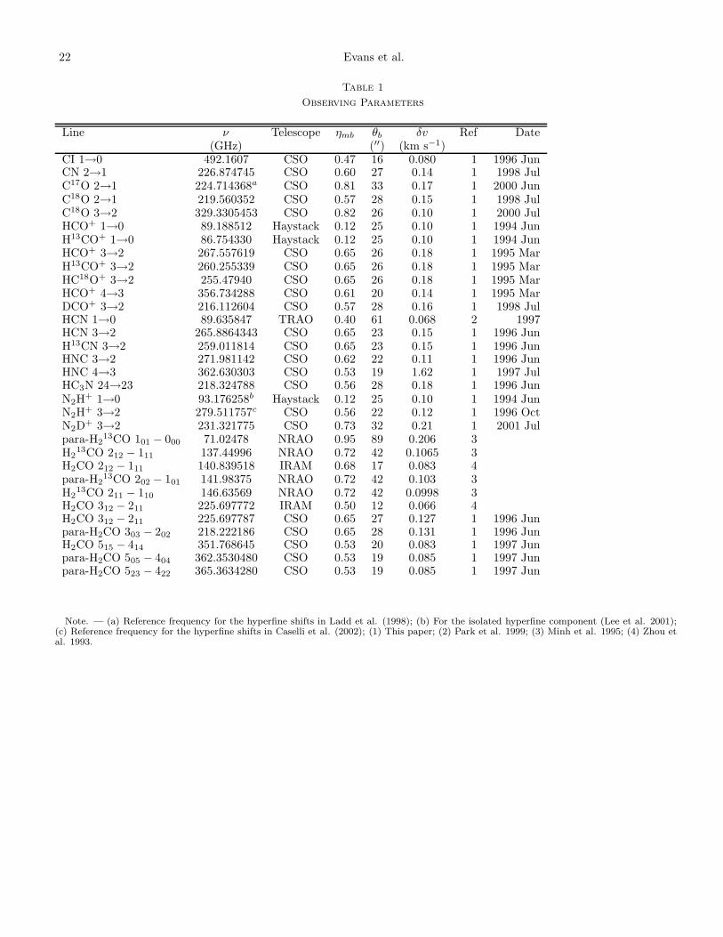
J = 1 → 0 lines at the Haystack Observatory in 1995March. Observations of a large number of lines were ob-tained at the Caltech Submillimeter Observatory in theperiod 1995 March to 2001 July. Table 1 provides the ref-erence frequency for the line, the telescope, the main beamefficiency (ηmb), the full width at half maximum beam size(θb), the velocity resolution (δv), and the date of observa-tion. We also provide this information for several obser-vations obtained previously that are used to constrain themodeling. The frequencies in Table 1 are either those usedduring observing or those used later to shift the observeddata to an improved rest frequency. For most lines withhyperfine components, these are the reference frequenciessuitable for a list of hyperfine components that were usedto fit lines. In the case of the N2H
+ J = 1 → 0 line, itis the frequency of the isolated hyperfine component, bestsuited for determining the velocity.
In the following sections, we assume that the centroidof B335 is at α = 19h34m35.4s; δ = 07◦27′24′′ in 1950coordinates. This position agrees within 1′′ with the cen-troid of the submillimeter emission mapped with SCUBA(Shirley et al. 2000). This position was originally basedon the position of the millimeter continuum source seenby Chandler & Sargent (1993); more recent interferomet-ric data find a compact component located 3.′′6 west and1′′ south of this position (Wilner et al. 2000). At this posi-tion, a continuum source is also seen at 3.6 cm, attributedto a time variable radio jet elongated along the outflowaxis (Reipurth et al. 2002). The difference between ourposition and the position of the compact component is notsignificant for the resolution of these observations. Some ofour data were obtained before we settled on this position.In cases where we have a map, we may have resampled thedata spatially to synthesize a spectrum at the submillime-ter centroid position, resulting in a slight degradation ofthe spatial resolution.
3. results
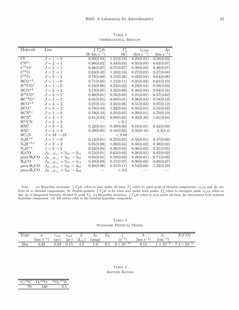
The primary observational results are presented in Ta-ble 2 and Figure 1 to Figure 7. The table gives the inte-grated intensity (
∫T ∗
Adv), the peak antenna temperature(T ∗
A), the velocity with respect to the local standard ofrest (vLSR), and the linewidth (FWHM), ∆v. For simple,
single-peaked lines, these were determined from a Gaus-sian fit. For self-reversed lines without hyperfine structure(HCO+ J = 1 → 0, J = 3 → 2, and J = 4 → 3),
∫T ∗
Adv isthe total area under the full line, T ∗
A is the strength of thestronger peak, vLSR is the velocity of the dip, determinedby eye, and ∆v is
∫T ∗
Adv divided by T ∗A. For lines with
hyperfine structure (C17O J = 2 → 1, N2D+ J = 3 → 2),∫
T ∗Adv gives the area under all the hyperfine components,
T ∗A gives the peak of the strongest, usually blended com-
ponents, and vLSR and ∆v come from a fit with all thehyperfine components. For the most complex situation,lines that are self-reversed, with hyperfine structure, vari-ous strategies were adopted. For CN J = 2 → 1,
∫T ∗
Adv,T ∗
A, and vLSR were determined as for double peaked lines,but ∆v was determined from an isolated component. Thespectrum of CN (Figure 6) clearly shows that the main hy-perfine line is self-reversed. For N2H
+ J = 1 → 0, all lineparameters were determined from the isolated componentat the frequency given in Table 1, as suggested by Lee,Myers, & Tafalla (2001).
The observations that are compared to full models areshown as solid lines in Figures 1 to 6. The CN J = 2 → 1spectrum in Figure 6 has not been modeled, and thedashed line is just a fit to the hyperfine components. Otherspectra that are not modeled in detail are shown in Figure7. These include spectra with complex hyperfine splittingthat we cannot model in detail and molecules without goodcollision rates.
The HCN J = 3 → 2 line is peculiar in that there is es-sentially no emission at velocities that would normally beassociated with the red part of the main hyperfine compo-nent. To ensure that this effect was not caused by emissionin the off position (10′ west), we took a deep integrationin the off position. No emission was seen at a level of 0.08K.
Single-peaked lines without overlapping hyperfine com-ponents provide the best measure of the rest velocity ofthe cloud. Based on those lines least likely to be opticallythick, the cloud velocity is 〈vLSR〉 = 8.30 ± 0.05 km s−1.For self-reversed lines, the mean velocity of the dip (de-termined by eye) is 〈vdip〉 = 8.41 ± 0.06 km s−1. All thevalues for vdip exceed those for 〈vLSR〉, by amounts rang-ing from 0.05 km s−1 to 0.25 km s−1. The mean shift,〈vdip − 〈vLSR〉〉 = 0.11 ± 0.07. Also, lines from higherJ levels have higher vdip than those from lower J levels,suggesting that the dip arises partially from inflowing gas.The three lines of HCO+, for example, have their dip at in-creasing velocity, with the J = 4 → 3 showing vdip = 8.55km s−1. This progression is similar to a pattern seen inCS lines toward IRAM04191 by Belloche et al. (2002).
4. the modeling procedure
We use the extensive observations described above totest models of the source. All the models are sphericalmodels with smooth (non-clumpy) density distributions.We focus on inside-out collapse models, though we discusssome variations on this basic model. All models includeself-consistent calculations of the dust and gas tempera-ture distributions (§4.1) and calculations of the molecularpopulations, radiative transport, and line formation (§4.3).Two kinds of models of the abundances as a function of ra-dius are used: step function models, and abundances from
B335: A Laboratory for Astrochemistry 3
an evolutionary chemical calculation (Lee et al. 2004), asdescribed in §4.2.
4.1. Determining Temperatures
The first step in comparing a physical model to observa-tions is to determine the temperatures that correspond toa particular density distribution. The dust temperaturescan be calculated self-consistently for a particular densitydistribution by various radiative transfer codes. We usedthe code of Egan et al. (1988) and the techniques describedby Shirley et al. (2002) for constraining parameters.
We assumed that dust opacities are given by column5 of the table in Ossenkopf & Henning (1994), known asOH5 opacities, because these have been shown to matchmany observations of star forming cores (e.g., Shirley et al.2002). One difference between the models by Shirley et al.and the current work is in the treatment of the interstellarradiation field (ISRF). In the previous work, we decreasedthe strength of the ISRF by a constant factor (sISRF ) atall wavelengths (except for the contribution of the cosmicmicrowave background). For B335, we used sISRF = 0.3.In the present work, we instead attenuate the ISRF us-ing the Draine & Lee (1984) extinction law and assumingAV = 1.3 mag. This procedure affects short wavelengthsmuch more than long wavelengths, leading to a somewhatless pronounced rise in dust temperature toward the out-side of the cloud. The choice of AV = 1.3 mag is somewhatarbitrary, but it accounts for the fact that molecules re-quire some dust shielding. It will also produce consistentresults when we consider the gas energetics.
Shirley et al. assumed an outer radius of 60,000 AU formost B335 models. We will mostly use an outer radius of0.15 pc (31,000 AU), as used by Choi et al. (1995). Studiesof the extinction as a function of impact parameter fromHST/NICMOS data are consistent with an outer radius ofabout this size (Harvey et al. 2001), in the sense that theextinction decrease with radius blends into the noise atthat radius. The choice of outer radius makes little differ-ence in most models. The inner radius for the dust modelsis taken to be 10−3 of the outer radius for the dust mod-els in order to capture the conversion of short-wavelengthradiation from the forming star and disk to longer wave-length radiation. The stellar temperature is set to 6000K, but this choice is completely irrelevant because of therapid conversion to longer wavelength radiation. The lu-minosity was set to 4.5 L⊙, which provided the best fit toa Shu model in Shirley et al. (2002).
Once we have a dust temperature distribution, Td(r),and a density distribution, n(r), we can compute the gastemperature distribution, TK(r). This was done with agas-dust energetics code written by S. Doty [see Doty &Neufeld (1997) and the appendix in Young et al. (2004) fordescriptions]. This code includes energy transfer betweengas and dust, heating by cosmic rays and the photoelectriceffect with PAHs, and molecular cooling.
The gas-dust energy transfer via collisions depends onthe total grain cross section per baryon, averaged over thedistribution of grain sizes (Σd). Following the discussionin the Appendix of Young et al. (2004), we take this valueto be 6.09 × 10⁻²² cm2. The cosmic ray heating dependson the cosmic ray ionization rate (ζ), which we take to be3 × 10−17 s−1 (van der Tak & van Dishoeck 2000). The
photoelectric heating follows the equation of Bakes & Tie-lens (1994), which includes heating from the photoelec-tric effect on very small grains. The rate depends on thestrength of the ultraviolet portion of the ISRF and the elec-tron density. Because this heating is only important on theoutside of the cloud, we set the electron density to 1 × 10⁻³
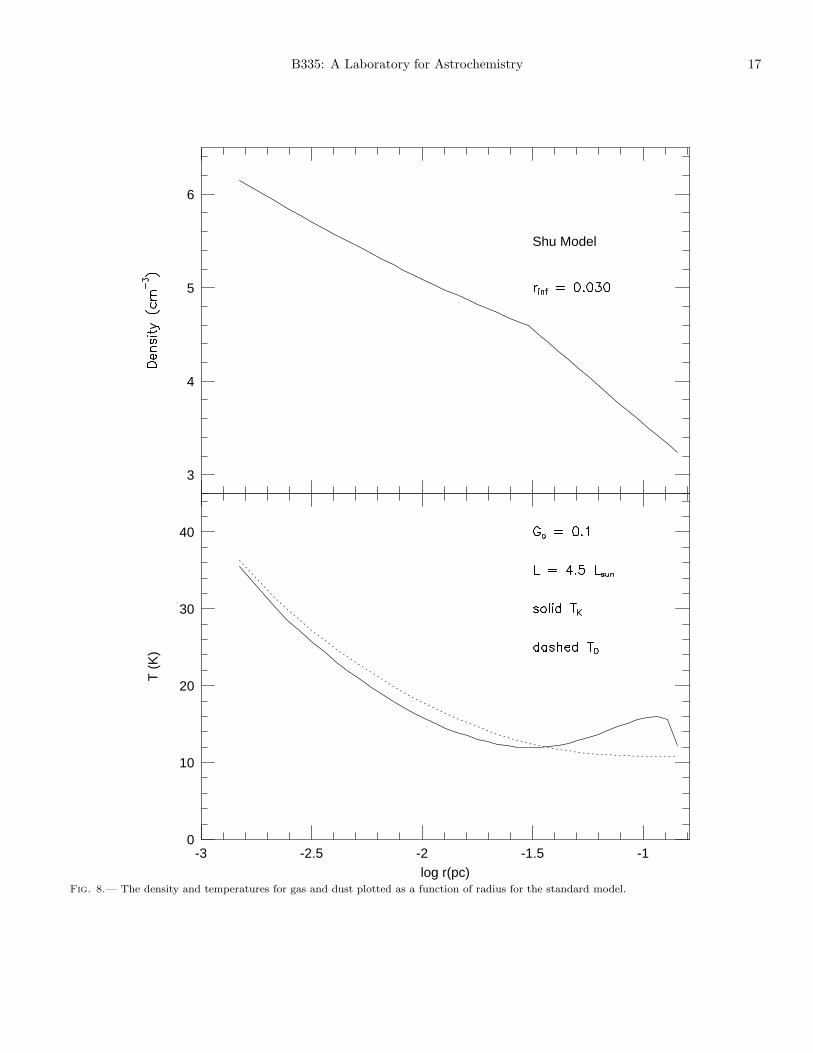
cm−3. The radiation field is assumed to be attenuated bythe surrounding medium according to τUV = 1.8AV ; withAV = 1.3, the scale factor for the ISRF impinging on ourmodel’s outer radius is G0 = 0.1. Once inside the cloud,the radiation is attenuated according to a fit to the atten-uation produced by the dust assumed to be in the cloud.
The result of these calculations is shown for a typicalmodel in Fig. 8. For small radii, TK ≈ Td, as is usuallyassumed, but TK falls below Td with increasing radius,as the density becomes too low for collisions with dustto maintain the kinetic temperature at the dust temper-ature. Then, at some radius, TK rises as photoelectricheating takes over, and TK > Td. The downturn in TK
at the cloud edge appears to be real and caused by thecooling lines of CO becoming optically thin (see Younget al. 2004). However, this drop in temperature has noappreciable effect on the resulting line profiles.
The amount of photoelectric heating is the least cer-tain of these inputs, as the external attenuation has alarge effect on how warm the outer cloud gets. To con-strain G0, we modeled the lower three lines of CO andcompared to data in the literature (e.g., Goldsmith et al.1984, Langer, Frerking, & Wilson 1986). To avoid pro-ducing a CO J = 1 → 0 line that exceeded the observa-tions, G0 definitely needed to be decreased from unity.The value of G0 = 0.1 provided the best match, and thiswas actually used to constrain the external extinction toAV = 1.3. Changes by a factor of 2 in G0 (or ±0.4 in AV )produced CO lines that differed from the observations byabout 30%, while having no appreciable effect on the linesof other species. While other variables are uncertain inthe photoelectric heating, the attenuation of the ultravi-olet radiation from the ISRF is the most important vari-able; comparison to observations of CO readily constrainit. The results are reasonable; one does not expect sig-nificant molecular gas for AV < 1 (van Dishoeck & Black1988). One could trade off the value of sISRF and theexternal extinction, as long as the effective G0 is not toodifferent from 0.1. Constraining these separately is diffi-cult (Shirley et al. 2004) and not particularly relevant forthis paper.
The cooling rates (Doty & Neufeld 1997) depend pri-marily on the CO abundance and the width of the lines(through trapping); we assume X(CO) = 7.4 × 10⁻⁵ andb = 0.12 km s−1, except for some tests described below.We note in passing the dangers of simplistic interpretationof observed CO lines; turning the observations into a ki-netic temperature would lead one to conclude that TK isconstant within the cloud, while it clearly is not.
The parameters that describe the standard physicalmodel are summarized in Table 3.
4.2. Chemical Modeling
Two kinds of abundance models are employed. The firstis strictly ad hoc, using a step function to describe theabundance of each species as a function of radius. These
4 Evans et al.
models have three free parameters per species: X , rdep,and fdep. The abundance in the outer parts of the cloud(X) is assumed to decrease inside a depletion radius (rdep)by a factor (fdep).
The second are true chemical models, based on the cal-culations presented by Lee et al. (2004). These calcula-tions follow the chemical evolution through an evolution-ary sequence that includes at each step a self-consistentcalculation of the dust and gas temperatures, using thetechniques described in the previous section. The evolu-tionary model assumes a slow build-up in central density,via a sequence of Bonnor-Ebert spheres, to the point ofa singular isothermal sphere, at which point, an inside-out collapse (Shu 1977) is initiated. After this point, thechemistry is calculated for each of 512 gas parcels as itfalls into the central region. Thus, gas inside the infallradius carries some memory of the conditions from fartherout. We adopt the model of Young and Evans (2004) forthe evolution of luminosity in order to calculate the evo-lution of dust temperature. Physical parameters in themodel are selected to have a total internal luminosity anda dust temperature profile similar to those obtained fromthe dust modeling of B335, at the time step of rinf = 0.03pc. The model core is assumed to stay in the same envi-ronment through its evolution with the same AV and G0
calculated in the previous section. The chemical calcula-tion includes the interaction between gas and dust grainsas well as gas-phase reactions, but the surface chemistryis not considered in the calculation. For details of thechemical evolution model, refer to Lee et al. (2004).
For both types of models, isotope ratios were con-strained so that the abundance was only a free parame-ter for the whole of the isotope complex. DCO+ was theexception, as it is subject to large fractionation effects.Assumed isotope ratios are the same as those used byJørgensen et al. (2004) and are given in Table 4. Wouter-loot et al. (2004) have recently suggested a slightly higherratio for 18O/17O of 4.1, but this value would fit our dataon the CO isotopologues somewhat worse.
4.3. Modeling of Line Profiles
The line profiles were modeled with a Monte Carlo code(mc) to calculate the excitation of the energy levels and avirtual telescope program (vt) to integrate along the line ofsight, convolve with a beam, and match the velocity reso-lution, spatial resolution, and main beam efficiency of theobservations (Choi et al. 1995). All lines were assumedto be centered at 8.30 km s−1, based on the average ofoptically thin lines.
The input physical conditions (density, temperature,and velocity fields) were taken from the physical modelbeing tested, using the results of the gas-dust energeticscode for TK(r). Models require input data about eachmolecule, as well as about the source. For CS, we usedcollision rates from Turner et al. (1992). For HCO+ andN2H
+, we used collision rates supplied by B. Turner, basedon his extension of previously calculated rates to highertemperatures and energy levels (Turner 1995). For H2COand para-H2CO, we used rates computed by Green (1991).Rates for HCN came from Green & Thaddeus (1974) andthose for CO from Flower & Launay (1985). In some cases,rates have been extrapolated to lower temperatures.
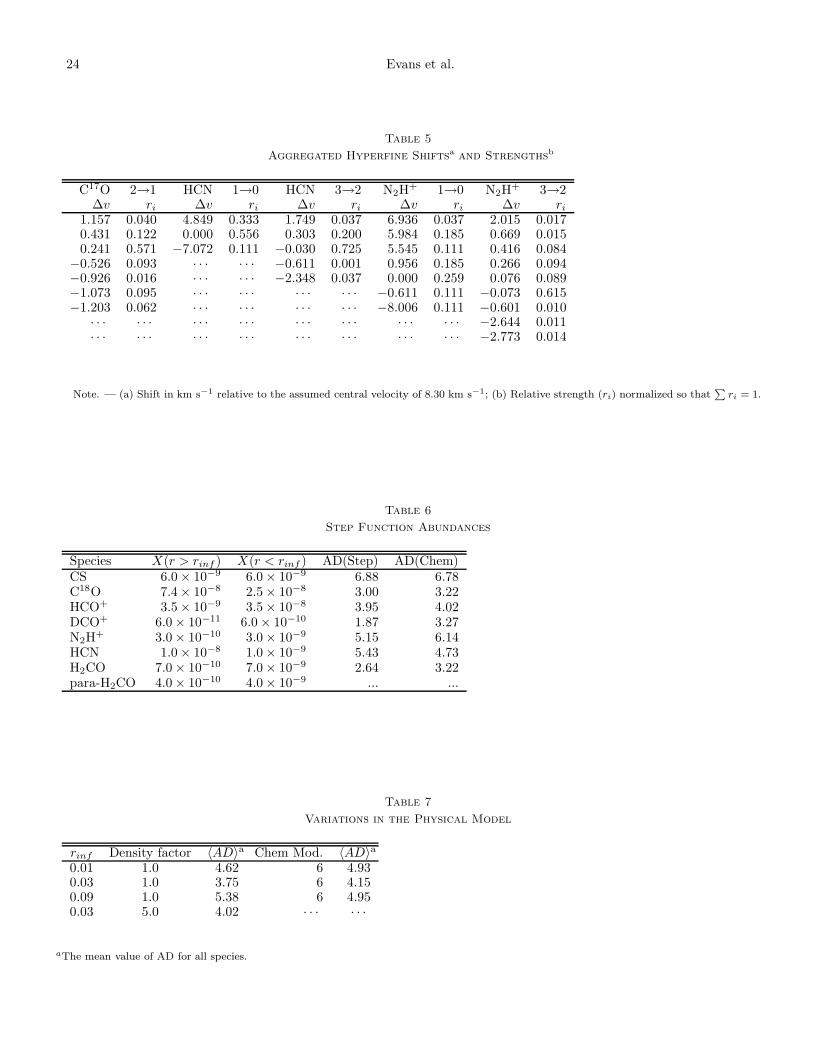
For C17O, HCN, and N2H+, the lines have hyperfine
structure that is partially resolved. For these lines, mc andvt models were run separately for each clearly resolved hy-perfine component, with abundances adjusted to simulatethe fraction of the transition probability in that compo-nent; the results were added to make the final simulatedline. Components separated by less than the 1/e width ofthe velocity dispersion were aggregated into a single com-ponent; the aggregated components are listed in Table 5.This procedure captures the essence of the hyperfine split-ting, but it is not rigorous because trapping is not handledcorrectly when there is partial line overlap (see Keto et al.2004).
All models were run with 40 shells. The inner radiuswas 2 × 10⁻³ pc, corresponding to 1.′′7 at a distance of250 pc. This radius is larger than the inner radius for thedust models because the molecular lines are not sensitiveto emission from very small scales because of beam dilu-tion. The convergence criterion for populations was setto 10% for finding the region of best-fitting parameters.Final models were run with a 2% convergence criterionto ensure accuracy; differences between these models andthose run with 10% accuracy were small. The minimumfractional population tested for convergence was 10−6. Foran explanation of these criteria, see the Appendix in Choiet al. (1995).
5. inside-out collapse models
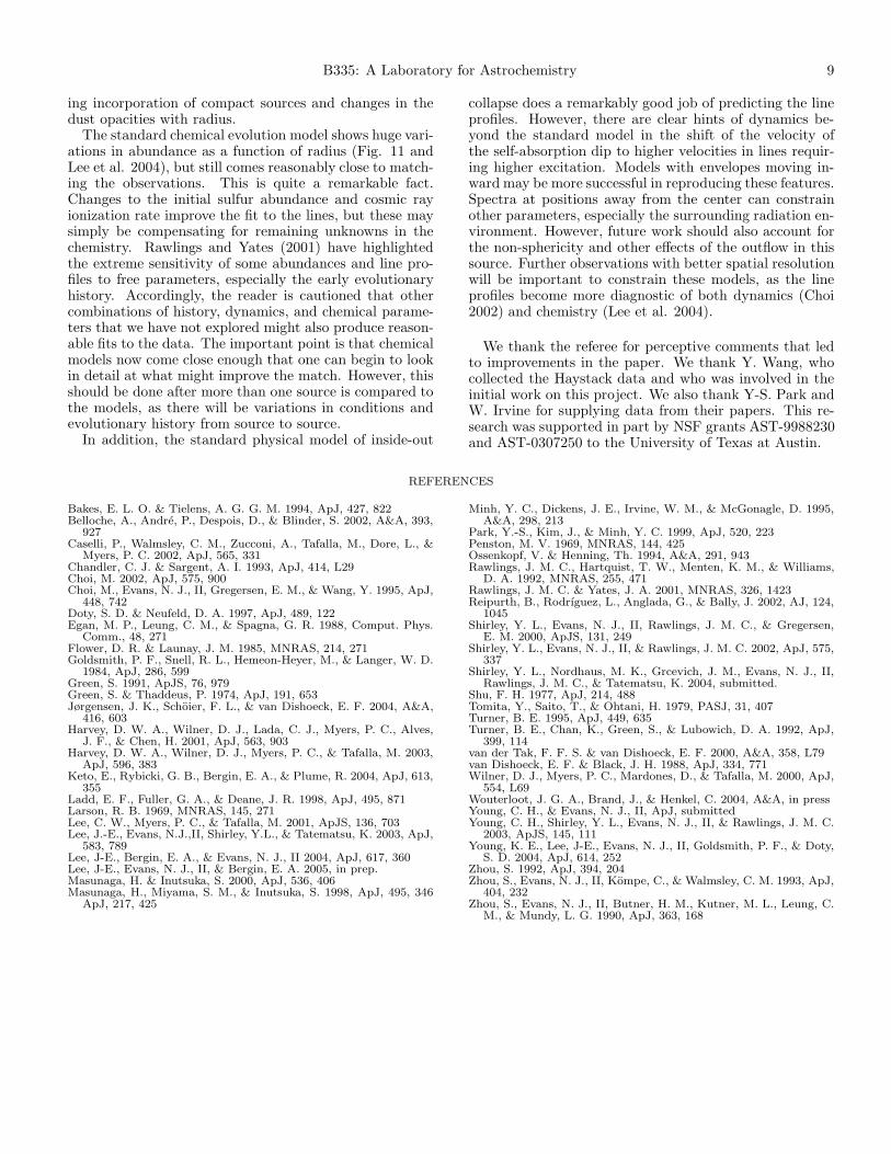
The physical properties of the standard model are givenin Table 3. The standard physical model is the inside-out collapse model (Shu 1977) that best matched (Choiet al. 1995) the CS and H2CO data taken by Zhou et al.(1993). Choi et al. (1995) modeled CS and H2CO linesfrom the IRAM telescope, assuming constant abundances,and found a best fit rinf = 0.03 pc. This was a compro-mise, as H2CO favored smaller rinf than did CS.
While the CS data were still well matched with constantabundance, the new data on more H2CO lines suggestedenhanced abundances on small scales, as did the HCO+
data. As a result, we tested step function abundance mod-els.
5.1. Step Function Abundances
To avoid too many free parameters, we required thatrdep = rinf . While this particular choice has no theoreticaljustification, it leaves only two free parameters per species.With the constraints on isotope ratios in Table 4, we areleft with 15 free parameters for 8 species, including the spe-cial case of DCO+, explained below. The abundances inTable 6 are those that fit the current data reasonably well,as judged by eye and statistical measures. We calculatedboth the reduced chi-squared (χ2
r) and the absolute devi-ation (AD =
∑i |T
∗A(model; i) − T ∗
A(obs; i)|/N) over theline profiles. The absolute deviation is more influenced bystrong lines for which the shape is important to match, sowe use it primarily, though the χ2
r criterion does not differin the choice of best model. We have not run a completegrid of models; instead, we employed some judgment to lo-cate regions of parameter space with decent fits to the lineprofiles. Once reasonably good fits were obtained, bothX and fdep were varied by factors of 3 in each direction,showing substantially worse fits. These parameters should
B335: A Laboratory for Astrochemistry 5
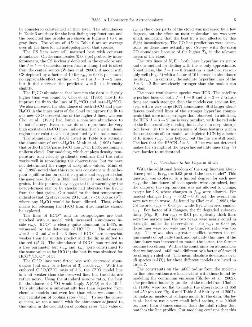
be considered constrained at that level. The abundancesin Table 6 are those for the best-fitting step functions, andthe predicted line profiles are shown in Figures 1 to 6 asgray lines. The values of AD in Table 6 are an averageover all the lines for all isotopologues of that species.
The CS lines were still matched best with constantabundance. On the small scales (0.003 pc) probed by inter-ferometers, the CS is clearly depleted in the envelope andthe J = 5 → 4 emission arises from a clump that is offsetfrom the central source (Wilner et al. 2000). A model withCS depleted by a factor of 10 for rdep = 0.003 pc showedno appreciable effect on the J = 2 → 1 or J = 3 → 2 lines,but it did decrease the predicted J = 5 → 4 intensityslightly.
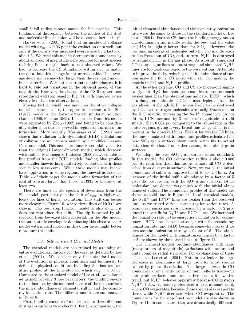
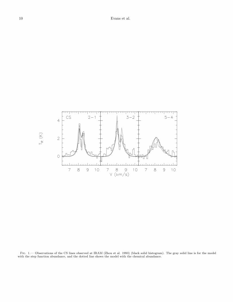
The H2CO abundance that best fits the data is slightlyhigher than was found by Choi et al. (1995), mostly toimprove the fit to the lines of H2
13CO and para-H213CO.
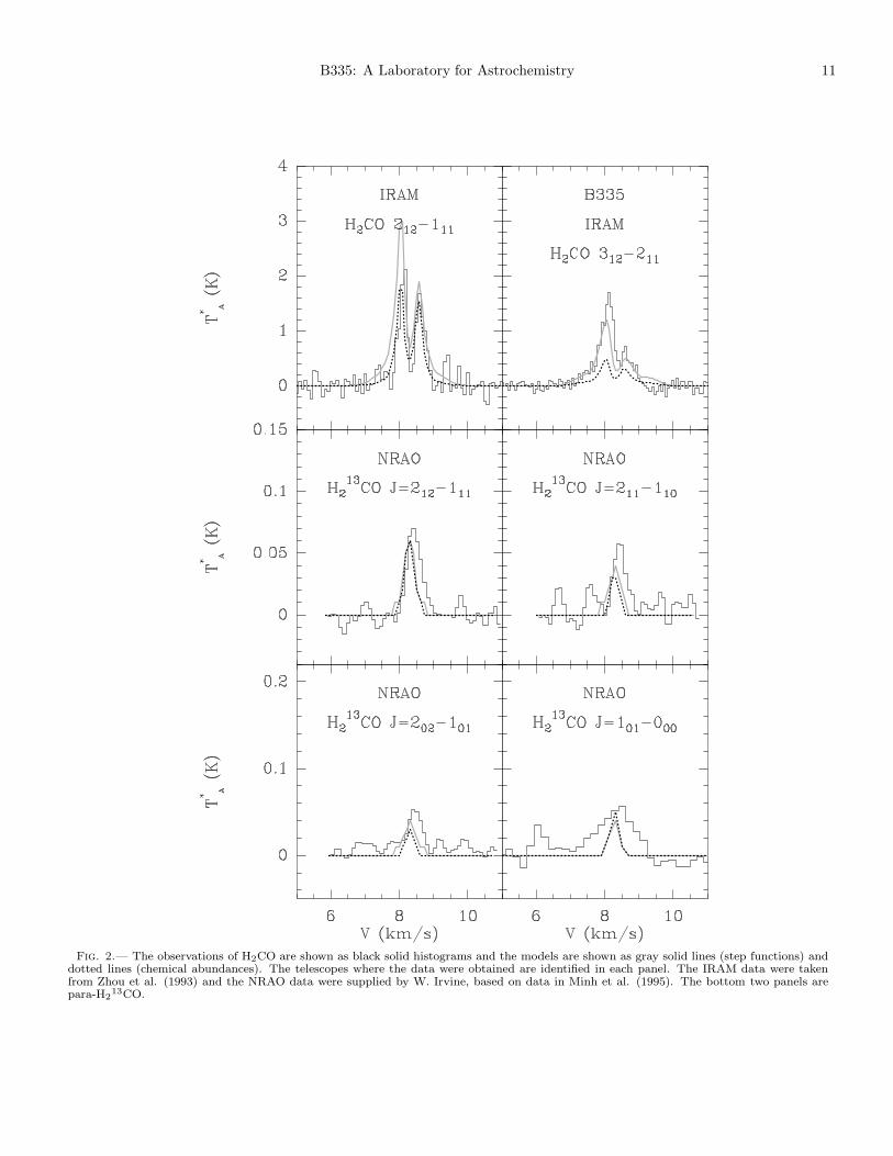
We also increased the abundance of both H2CO and para-H2CO in the inner parts of the cloud to improve the fit toour new CSO observations of the higher-J lines, whereasChoi et al. (1995) had found a constant abundance tobe satisfactory. Even so, we do not reproduce the veryhigh excitation H2CO lines, indicating that a warm, denseregion must exist that is not predicted by the basic model.
The abundance of H2CO listed in Table 6 is actuallythe abundance of ortho-H2CO. Minh et al. (1995) foundthat ortho-H2CO/para-H2CO was 1.7 in B335, assuming auniform cloud. Our modeling, which employs density, tem-perature, and velocity gradients, confirms that this ratioworks well in reproducing the observations, but we havenot determined the range of acceptable values. Minh etal. (1995) noted that this ratio was consistent with ortho-para equilibration on cold dust grains and suggested thatthe gas-phase H2CO in B335 had formerly resided on dustgrains. In this picture, they suggested that warming by thenewly-formed star or by shocks had liberated the H2COfrom the dust grains. Our model for the dust temperatureindicates that Td stays below 20 K until r < 0.006 pc (6′′),where any H2CO would be beam diluted. Thus, othermeans for releasing the H2CO from dust mantles shouldbe explored.
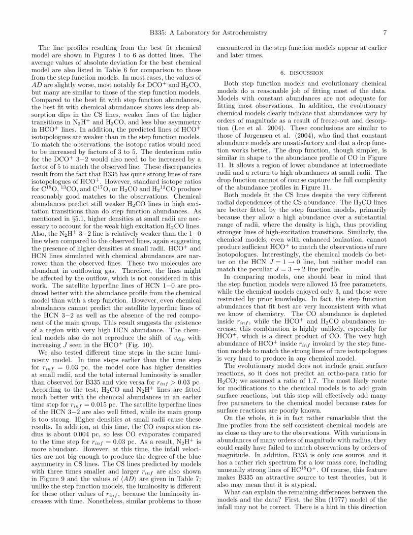
The lines of HCO+ and its isotopologues are bestmatched with a model with increased abundances in-side rinf . HCO+ is clearly quite abundant in B335, aswitnessed by the detection of HC18O+. The observedJ = 3 → 2 and J = 4 → 3 lines of HCO+ are somewhatweaker than the models predict and the dip is shifted tothe red (§5.2). The abundance of DCO+ was treated asa free parameter but rdep and fdep were constrained tothe same value as for HCO+; the best fit was obtained forHCO+/DCO+ of 55.
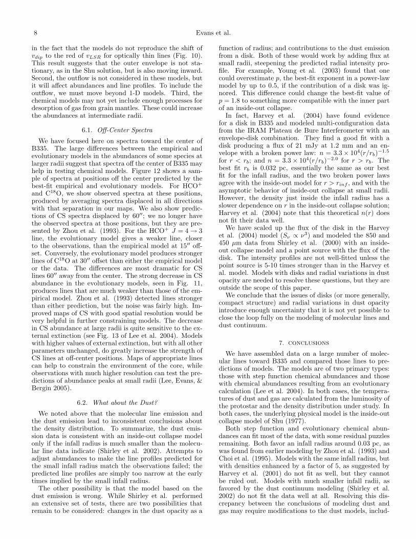
The C18O lines were fitted best with decreased abun-dances (but only by a factor of 3) inside rinf . With theenforced C18O/C17O ratio of 3.5, the C17O model lineis a bit weaker than the observed line, but the data arerather noisy. Using the standard isotope ratio, the bestfit abundance of C18O would imply X(CO) = 4 × 10⁻⁵.This abundance is substantially less than expected fromchemical models and even less than what we assume inour calculation of cooling rates (§4.1). To see the conse-quences, we ran a model with the abundance adjusted tothis value in the calculation of cooling rates. The value of
TK in the outer parts of the cloud was increased by a fewdegrees, but the effect on most molecular lines was verysmall, indicating that the best fit is not affected by thisslight inconsistency. The CO line predictions were excep-tions, as these lines actually got stronger with decreasedCO abundance because of the higher TK in the relevantlayers of the cloud.
The two lines of N2H+ both have hyperfine structure
and our method for dealing with this is only approximate.Nonetheless, the J = 1 → 0 transition is matched reason-ably well (Fig. 6) with a factor of 10 increase in abundanceinside rinf . In contrast, the satellite hyperfine lines of theJ = 3 → 2 line are clearly stronger than the models canexplain.
The most troublesome species was HCN. The satellitehyperfine lines of both J = 1 → 0 and J = 3 → 2 transi-tions are much stronger than the models can account for,even with a very large HCN abundance. Still larger abun-dances predicted lines of the stronger hyperfine compo-nents that were much stronger than observed. In addition,the HCN J = 3 → 2 line is very peculiar, with the red sideof the line essentially missing, indicative of a deep absorp-tion layer. To try to match some of these features withinthe constraints of our model, we depleted HCN by a factorof 10 inside rinf . This helped, but the fits are still poor.The fact that the H13CN J = 3 → 2 line was not detectedmakes the strength of the hyperfine satellite lines (Fig. 7)even harder to understand.
5.2. Variations in the Physical Model
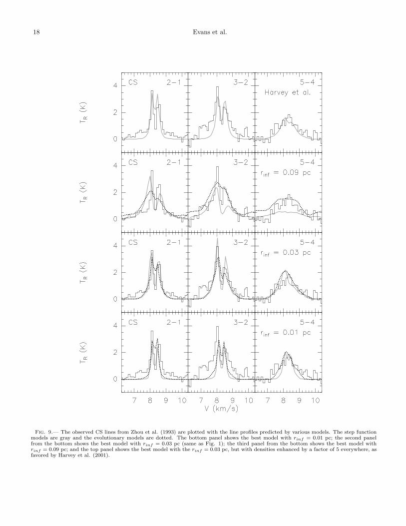
With the additional freedom of the step function abun-dance profile, is rinf = 0.03 pc still the best model? Thisquestion was explored to a limited degree; for each newrinf , the abundances of each species were optimized, butthe shape of the step function was not allowed to change,except for CS, where changes in fdep were allowed. Formodest changes (rinf = 0.02 − 0.04 pc), the overall fitswere not much worse. As found by Choi et al. (1995), theCS favored rinf = 0.03 pc, while H2CO favored smallerrinf . For factor of 3 changes, the fit degraded substan-tially (Fig. 9). For rinf = 0.01 pc, optically thick lineswere too narrow and the two peaks were nearly equal instrength, unlike the observations. For rinf = 0.09 pc,those lines were too wide and the blue/red ratio was toolarge. There was also a greater conflict between the re-quirements of optically thick and optically thin lines; if theabundance was increased to match the latter, the formerbecame too strong. Within the constraints on abundancesthat we imposed, infall radii different by a factor of 3 wouldbe strongly ruled out. The mean absolute deviations overall species (〈AD〉) for these different models are listed inTable 7.
The constraints on the infall radius from the molecu-lar line observations are inconsistent with those found bymodeling the continuum emission (Shirley et al. 2002).The predicted intensity profiles of the model from Choi etal. (1995) were too flat to match the observations at 850and 450 µm (see Fig. 6 and Table 3 of Shirley et al 2002).To make an inside-out collapse model fit the data, Shirleyet al. had to use a very small infall radius, r = 0.0048pc, more than 6 times smaller than the infall radius thatmatches the line profiles. Our modeling confirms that this
6 Evans et al.
small infall radius cannot match the line profiles. Thisfundamental discrepancy between the models of the dustand molecular line emission will be discussed further in §6.
Harvey et al. (2001) found that an inside-out collapsemodel with rinf ∼ 0.03 pc fit the extinction data well, butonly if the density was increased everywhere by a factor ofabout 5. We tried this model; decreases in abundances byabout an order of magnitude were required for most speciesto bring line strengths back to near observed values. Wehad to decrease the CS abundance within rdep to matchthe data, but this change is not unreasonable. The aver-age deviation is somewhat larger than the standard model,but not terrible. Without constraints on abundances, it ishard to rule out variations in the physical model of thismagnitude. However, the shapes of the CS lines were notreproduced well (top panel in Fig. 9), with blue/red ratiosclearly less than the observations.
Moving farther afield, one may consider other collapsemodels. In some sense, the opposite extreme to the Shu(1977) model is the Larson-Penston similarity solution(Larson 1969, Penston 1969). Line profiles from this modelwere generated by Zhou (1992) and found to be consider-ably wider than those observed in regions of low-mass starformation. More recently, Masunaga et al. (1998) haveshown that radiation hydrodynamical (RHD) calculationsof collapse are well approximated by a modified Larson-Penston model. This model produces lower infall velocitiesthan the original Larson-Penston model, which decreasewith radius. Masunaga & Inutsuka (2000) have simulatedline profiles from the RHD models, finding blue profilesand smaller linewidths, qualitatively consistent with thoseseen in low mass cores. While these models may indeedhave application in some regions, the linewidths listed inTable 4 of their paper for models after formation of thecentral core are larger than those in B335 by factors of atleast two.
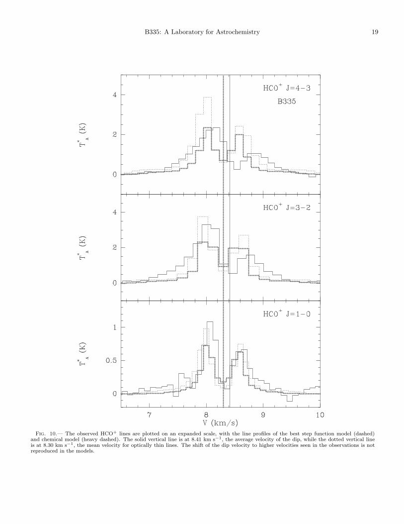
There are hints in the spectra of deviations from theShu model, particularly in the shift of vdip to higher ve-locity for lines of higher excitation. This shift can be seemore clearly in Figure 10, where three lines of HCO+ areshown. The best step function model is also shown; itdoes not reproduce this shift. The dip is caused by ab-sorption from low-excitation material. In the Shu model,the outer, static envelope is dominating this absorption. Amodel with inward motion in this outer layer might betterreproduce this shift.
5.3. Self-consistent Chemical Models
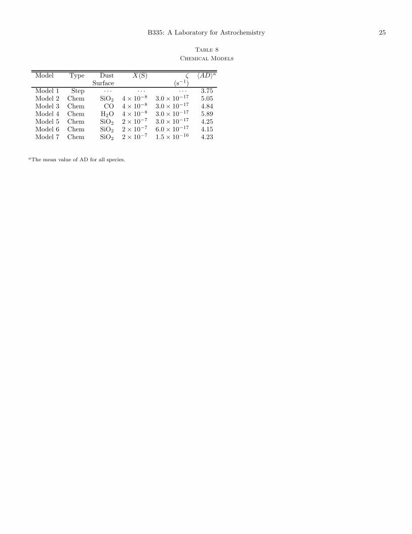
The chemical models are constrained by assuming anentire evolutionary history for the core, as detailed by Leeet al. (2004). We consider only their standard modelof the evolution of physical conditions and luminosity todefine the physical conditions, including the dust temper-ature profile, at the time step for which rinf = 0.03 pc.Compared to the standard model of Lee et al., we allowedadjustment of only 3 free parameters: the binding energyto the dust, set by the assumed nature of the dust surface;the initial abundance of elemental sulfur; and the cosmic-ray ionization rate. The different models are summarizedin Table 8.
First, binding energies of molecules onto three differentdust grain surfaces were checked. For this comparison, the
initial elemental abundances and the cosmic-ray ionizationrate were the same as those in the standard model of Leeet al. (2004). For the CS lines, the binding energy onto aCO-dominant grain mantle works the best and the valueof 〈AD〉 is slightly better than for SiO2. However, thelow binding energy of molecules onto the CO mantle leadsto less freeze-out of CO, and, in turn, N2H
+ is destroyedby abundant CO in the gas phase. As a result, simulatedCO isotopologue lines are too strong, and simulated N2H
+
lines are too weak compared to the observations. Attemptsto improve the fit by reducing the initial abundance of car-bon make the fit to CS worse while still not making themodels fit CO and N2H
+ profiles.At the other extreme, CO and CS are frozen-out signifi-
cantly onto H2O-dominant grain mantles to produce muchweaker lines than the observations indicate. HCO+, whichis a daughter molecule of CO, is also depleted from thegas phase. Although N2H
+ is less likely to be destroyedby CO, even nitrogen molecules are easily frozen-out onthe H2O mantle, decreasing the N2H
+ abundance. In ad-dition, HCN increases by 3 orders of magnitude at radiismaller than 0.004 pc, compared to the abundance in theouter regions, giving a very broad line wing, which is notpresent in the observed lines. Except for weaker CS lines,the lines simulated with abundance profiles calculated forbare SiO2 grain surfaces show much better fits to actualdata than do those from other assumptions about grainsurfaces.
We adopt the bare SiO2 grain surface as our standard.In this model, the CO evaporation radius is about 0.006pc. At radii less than this radius, almost all CO is des-orbed from dust grain surfaces. Next, we varied the initialabundance of sulfur to improve the fit to the CS lines. Anincrease of the initial sulfur abundance by a factor of 5gives the best results with the SiO2 grain surfaces. Othermolecular lines do not vary much with the initial abun-dance of sulfur. The abundance profiles of this model areshown as solid lines in Figure 11. In all chemical models,the N2H
+ and HCO+ lines are weaker than the observedlines, so we tested various cosmic-ray ionization rates. Acosmic-ray ionization rate increased by a factor of 2 pro-duced the best fit for N2H
+ and HCO+ lines. We increasedthe ionization rate in the energetics calculation for consis-tency. HCN lines become stronger with the cosmic-rayionization rate, and 〈AD〉 becomes somewhat worse if weincrease the ionization rate by a factor of 5. The abun-dances for the model with ionization enhanced by a factorof 2 are shown by the dotted lines in Figure 11.
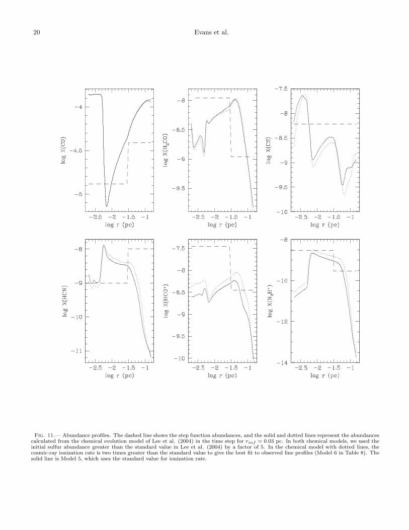
The chemical models produce abundances with large(many orders of magnitude) variations with radius andquite complex radial structure. For explanations of theseeffects, see Lee et al. (2004). Note in particular the largedecreases in abundance at large radii for most speciescaused by photo-dissociation. The large decrease in COabundance over a wide range of radii reflects freeze-outonto grain surfaces, and some other species follow thistrend, but N2H
+ behaves oppositely because CO destroysN2H
+. Likewise, most species show a peak at small radii,where CO evaporates, because those species also evaporatethere, while N2H
+ decreases when CO evaporates. Theabundances for the step function model are also shown inFigure 11. In some cases, they are dramatically different.
B335: A Laboratory for Astrochemistry 7
The line profiles resulting from the best fit chemicalmodel are shown in Figures 1 to 6 as dotted lines. Theaverage values of absolute deviation for the best chemicalmodel are also listed in Table 6 for comparison to thosefrom the step function models. In most cases, the values ofAD are slightly worse, most notably for DCO+ and H2CO,but many are similar to those of the step function models.Compared to the best fit with step function abundances,the best fit with chemical abundances shows less deep ab-sorption dips in the CS lines, weaker lines of the highertransitions in N2H
+ and H2CO, and less blue asymmetryin HCO+ lines. In addition, the predicted lines of HCO+
isotopologues are weaker than in the step function models.To match the observations, the isotope ratios would needto be increased by factors of 3 to 5. The deuterium ratiofor the DCO+ 3−2 would also need to be increased by afactor of 5 to match the observed line. These discrepanciesresult from the fact that B335 has quite strong lines of rareisotopologues of HCO+. However, standard isotope ratiosfor C18O, 13CO, and C17O, or H2CO and H2
13CO producereasonably good matches to the observations. Chemicalabundances predict still weaker H2CO lines in high exci-tation transitions than do step function abundances. Asmentioned in §5.1, higher densities at small radii are nec-essary to account for the weak high excitation H2CO lines.Also, the N2H
+ 3−2 line is relatively weaker than the 1−0line when compared to the observed lines, again suggestingthe presence of higher densities at small radii. HCO+ andHCN lines simulated with chemical abundances are nar-rower than the observed lines. These two molecules areabundant in outflowing gas. Therefore, the lines mightbe affected by the outflow, which is not considered in thiswork. The satellite hyperfine lines of HCN 1−0 are pro-duced better with the abundance profile from the chemicalmodel than with a step function. However, even chemicalabundances cannot predict the satellite hyperfine lines ofthe HCN 3−2 as well as the absence of the red compo-nent of the main group. This result suggests the existenceof a region with very high HCN abundance. The chem-ical models also do not reproduce the shift of vdip withincreasing J seen in the HCO+ (Fig. 10).
We also tested different time steps in the same lumi-nosity model. In time steps earlier than the time stepfor rinf = 0.03 pc, the model core has higher densitiesat small radii, and the total internal luminosity is smallerthan observed for B335 and vice versa for rinf > 0.03 pc.According to the test, H2CO and N2H
+ lines are fittedmuch better with the chemical abundances in an earliertime step for rinf = 0.015 pc. The satellite hyperfine linesof the HCN 3−2 are also well fitted, while its main groupis too strong. Higher densities at small radii cause theseresults. In addition, at this time, the CO evaporation ra-dius is about 0.004 pc, so less CO evaporates comparedto the time step for rinf = 0.03 pc. As a result, N2H
+ ismore abundant. However, at this time, the infall veloci-ties are not big enough to produce the degree of the blueasymmetry in CS lines. The CS lines predicted by modelswith three times smaller and larger rinf are also shownin Figure 9 and the values of 〈AD〉 are given in Table 7;unlike the step function models, the luminosity is differentfor these other values of rinf , because the luminosity in-creases with time. Nonetheless, similar problems to those
encountered in the step function models appear at earlierand later times.
6. discussion
Both step function models and evolutionary chemicalmodels do a reasonable job of fitting most of the data.Models with constant abundances are not adequate forfitting most observations. In addition, the evolutionarychemical models clearly indicate that abundances vary byorders of magnitude as a result of freeze-out and desorp-tion (Lee et al. 2004). These conclusions are similar tothose of Jørgensen et al. (2004), who find that constantabundance models are unsatisfactory and that a drop func-tion works better. The drop function, though simpler, issimilar in shape to the abundance profile of CO in Figure11. It allows a region of lower abundance at intermediateradii and a return to high abundances at small radii. Thedrop function cannot of course capture the full complexityof the abundance profiles in Figure 11.
Both models fit the CS lines despite the very differentradial dependences of the CS abundance. The H2CO linesare better fitted by the step function models, primarilybecause they allow a high abundance over a substantialrange of radii, where the density is high, thus providingstronger lines of high-excitation transitions. Similarly, thechemical models, even with enhanced ionization, cannotproduce sufficient HCO+ to match the observations of rareisotopologues. Interestingly, the chemical models do bet-ter on the HCN J = 1 → 0 line, but neither model canmatch the peculiar J = 3 → 2 line profile.
In comparing models, one should bear in mind thatthe step function models were allowed 15 free parameters,while the chemical models enjoyed only 3, and those wererestricted by prior knowledge. In fact, the step functionabundances that fit best are very inconsistent with whatwe know of chemistry. The CO abundance is depletedinside rinf , while the HCO+ and H2CO abundances in-crease; this combination is highly unlikely, especially forHCO+, which is a direct product of CO. The very highabundance of HCO+ inside rinf invoked by the step func-tion models to match the strong lines of rare isotopologuesis very hard to produce in any chemical model.
The evolutionary model does not include grain surfacereactions, so it does not predict an ortho-para ratio forH2CO; we assumed a ratio of 1.7. The most likely routefor modifications to the chemical models is to add grainsurface reactions, but this step will effectively add manyfree parameters to the chemical model because rates forsurface reactions are poorly known.
On the whole, it is in fact rather remarkable that theline profiles from the self-consistent chemical models areas close as they are to the observations. With variations inabundances of many orders of magnitude with radius, theycould easily have failed to match observations by orders ofmagnitude. In addition, B335 is only one source, and ithas a rather rich spectrum for a low mass core, includingunusually strong lines of HC18O+. Of course, this featuremakes B335 an attractive source to test theories, but italso may mean that it is atypical.
What can explain the remaining differences between themodels and the data? First, the Shu (1977) model of theinfall may not be correct. There is a hint in this direction
8 Evans et al.
in the fact that the models do not reproduce the shift ofvdip to the red of vLSR for optically thin lines (Fig. 10).This result suggests that the outer envelope is not sta-tionary, as in the Shu solution, but is also moving inward.Second, the outflow is not considered in these models, butit will affect abundances and line profiles. To include theoutflow, we must move beyond 1-D models. Third, thechemical models may not yet include enough processes fordesorption of gas from grain mantles. These could increasethe abundances at intermediate radii.
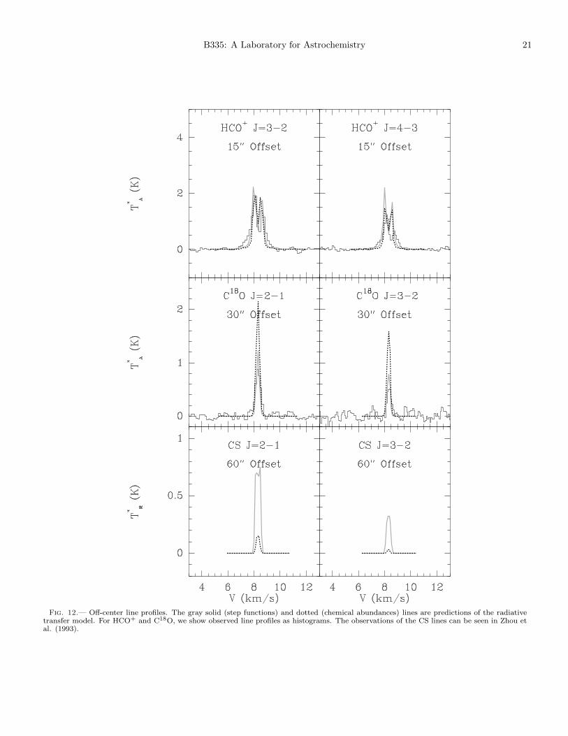
6.1. Off-Center Spectra
We have focused here on spectra toward the center ofB335. The large differences between the empirical andevolutionary models in the abundances of some species atlarger radii suggest that spectra off the center of B335 mayhelp in testing chemical models. Figure 12 shows a sam-ple of spectra at positions off the center predicted by thebest-fit empirical and evolutionary models. For HCO+
and C18O, we show observed spectra at these positions,produced by averaging spectra displaced in all directionswith that separation in our maps. We also show predic-tions of CS spectra displaced by 60′′; we no longer havethe observed spectra at those positions, but they are pre-sented by Zhou et al. (1993). For the HCO+ J = 4 → 3line, the evolutionary model gives a weaker line, closerto the observations, than the empirical model at 15′′ off-set. Conversely, the evolutionary model produces strongerlines of C18O at 30′′ offset than either the empirical modelor the data. The differences are most dramatic for CSlines 60′′ away from the center. The strong decrease in CSabundance in the evolutionary models, seen in Fig. 11,produces lines that are much weaker than those of the em-pirical model. Zhou et al. (1993) detected lines strongerthan either prediction, but the noise was fairly high. Im-proved maps of CS with good spatial resolution would bevery helpful in further constraining models. The decreasein CS abundance at large radii is quite sensitive to the ex-ternal extinction (see Fig. 13 of Lee et al. 2004). Modelswith higher values of external extinction, but with all otherparameters unchanged, do greatly increase the strength ofCS lines at off-center positions. Maps of appropriate linescan help to constrain the environment of the core, whileobservations with much higher resolution can test the pre-dictions of abundance peaks at small radii (Lee, Evans, &Bergin 2005).
6.2. What about the Dust?
We noted above that the molecular line emission andthe dust emission lead to inconsistent conclusions aboutthe density distribution. To summarize, the dust emis-sion data is consistent with an inside-out collapse modelonly if the infall radius is much smaller than the molecu-lar line data indicate (Shirley et al. 2002). Attempts toadjust abundances to make the line profiles predicted forthe small infall radius match the observations failed; thepredicted line profiles are simply too narrow at the earlytimes implied by the small infall radius.
The other possibility is that the model based on thedust emission is wrong. While Shirley et al. performedan extensive set of tests, there are two possibilities thatremain to be considered: changes in the dust opacity as a
function of radius; and contributions to the dust emissionfrom a disk. Both of these would work by adding flux atsmall radii, steepening the predicted radial intensity pro-file. For example, Young et al. (2003) found that onecould overestimate p, the best-fit exponent in a power-lawmodel by up to 0.5, if the contribution of a disk was ig-nored. This difference could change the best-fit value ofp = 1.8 to something more compatible with the inner partof an inside-out collapse.
In fact, Harvey et al. (2004) have found evidencefor a disk in B335 and modeled multi-configuration datafrom the IRAM Plateau de Bure Interferometer with anenvelope-disk combination. They find a good fit with adisk producing a flux of 21 mJy at 1.2 mm and an en-velope with a broken power law: n = 3.3 × 10⁴(r/rb)
−1.5
for r < rb; and n = 3.3 × 10⁴(r/rb)−2.0 for r > rb. The
best fit rb is 0.032 pc, essentially the same as our bestfit for the infall radius, and the two broken power lawsagree with the inside-out model for r > rinf , and with theasymptotic behavior of inside-out collapse at small radii.However, the density just inside the infall radius has aslower dependence on r in the inside-out collapse solution;Harvey et al. (2004) note that this theoretical n(r) doesnot fit their data well.
We have scaled up the flux of the disk in the Harveyet al. (2004) model (Sν ∝ ν3) and modeled the 850 and450 µm data from Shirley et al. (2000) with an inside-out collapse model and a point source with the flux of thedisk. The intensity profiles are not well-fitted unless thepoint source is 5-10 times stronger than in the Harvey etal. model. Models with disks and radial variations in dustopacity are needed to resolve these questions, but they areoutside the scope of this paper.
We conclude that the issues of disks (or more generally,compact structure) and radial variations in dust opacityintroduce enough uncertainty that it is not yet possible toclose the loop fully on the modeling of molecular lines anddust continuum.
7. conclusions
We have assembled data on a large number of molec-ular lines toward B335 and compared those lines to pre-dictions of models. The models are of two primary types:those with step function chemical abundances and thosewith chemical abundances resulting from an evolutionarycalculation (Lee et al. 2004). In both cases, the tempera-tures of dust and gas are calculated from the luminosity ofthe protostar and the density distribution under study. Inboth cases, the underlying physical model is the inside-outcollapse model of Shu (1977).
Both step function and evolutionary chemical abun-dances can fit most of the data, with some residual puzzlesremaining. Both favor an infall radius around 0.03 pc, aswas found from earlier modeling by Zhou et al. (1993) andChoi et al. (1995). Models with the same infall radius, butwith densities enhanced by a factor of 5, as suggested byHarvey et al. (2001) do not fit as well, but they cannotbe ruled out. Models with much smaller infall radii, asfavored by the dust continuum modeling (Shirley et al.2002) do not fit the data well at all. Resolving this dis-crepancy between the conclusions of modeling dust andgas may require modifications to the dust models, includ-
B335: A Laboratory for Astrochemistry 9
ing incorporation of compact sources and changes in thedust opacities with radius.
The standard chemical evolution model shows huge vari-ations in abundance as a function of radius (Fig. 11 andLee et al. 2004), but still comes reasonably close to match-ing the observations. This is quite a remarkable fact.Changes to the initial sulfur abundance and cosmic rayionization rate improve the fit to the lines, but these maysimply be compensating for remaining unknowns in thechemistry. Rawlings and Yates (2001) have highlightedthe extreme sensitivity of some abundances and line pro-files to free parameters, especially the early evolutionaryhistory. Accordingly, the reader is cautioned that othercombinations of history, dynamics, and chemical parame-ters that we have not explored might also produce reason-able fits to the data. The important point is that chemicalmodels now come close enough that one can begin to lookin detail at what might improve the match. However, thisshould be done after more than one source is compared tothe models, as there will be variations in conditions andevolutionary history from source to source.
In addition, the standard physical model of inside-out
collapse does a remarkably good job of predicting the lineprofiles. However, there are clear hints of dynamics be-yond the standard model in the shift of the velocity ofthe self-absorption dip to higher velocities in lines requir-ing higher excitation. Models with envelopes moving in-ward may be more successful in reproducing these features.Spectra at positions away from the center can constrainother parameters, especially the surrounding radiation en-vironment. However, future work should also account forthe non-sphericity and other effects of the outflow in thissource. Further observations with better spatial resolutionwill be important to constrain these models, as the lineprofiles become more diagnostic of both dynamics (Choi2002) and chemistry (Lee et al. 2004).
We thank the referee for perceptive comments that ledto improvements in the paper. We thank Y. Wang, whocollected the Haystack data and who was involved in theinitial work on this project. We also thank Y-S. Park andW. Irvine for supplying data from their papers. This re-search was supported in part by NSF grants AST-9988230and AST-0307250 to the University of Texas at Austin.
REFERENCES
Bakes, E. L. O. & Tielens, A. G. G. M. 1994, ApJ, 427, 822Belloche, A., Andre, P., Despois, D., & Blinder, S. 2002, A&A, 393,
927Caselli, P., Walmsley, C. M., Zucconi, A., Tafalla, M., Dore, L., &
Myers, P. C. 2002, ApJ, 565, 331Chandler, C. J. & Sargent, A. I. 1993, ApJ, 414, L29Choi, M. 2002, ApJ, 575, 900Choi, M., Evans, N. J., II, Gregersen, E. M., & Wang, Y. 1995, ApJ,
448, 742Doty, S. D. & Neufeld, D. A. 1997, ApJ, 489, 122Egan, M. P., Leung, C. M., & Spagna, G. R. 1988, Comput. Phys.
Comm., 48, 271Flower, D. R. & Launay, J. M. 1985, MNRAS, 214, 271Goldsmith, P. F., Snell, R. L., Hemeon-Heyer, M., & Langer, W. D.
1984, ApJ, 286, 599Green, S. 1991, ApJS, 76, 979Green, S. & Thaddeus, P. 1974, ApJ, 191, 653Jørgensen, J. K., Schoier, F. L., & van Dishoeck, E. F. 2004, A&A,
416, 603Harvey, D. W. A., Wilner, D. J., Lada, C. J., Myers, P. C., Alves,
J. F., & Chen, H. 2001, ApJ, 563, 903Harvey, D. W. A., Wilner, D. J., Myers, P. C., & Tafalla, M. 2003,
ApJ, 596, 383Keto, E., Rybicki, G. B., Bergin, E. A., & Plume, R. 2004, ApJ, 613,
355Ladd, E. F., Fuller, G. A., & Deane, J. R. 1998, ApJ, 495, 871Larson, R. B. 1969, MNRAS, 145, 271Lee, C. W., Myers, P. C., & Tafalla, M. 2001, ApJS, 136, 703Lee, J.-E., Evans, N.J.,II, Shirley, Y.L., & Tatematsu, K. 2003, ApJ,
583, 789Lee, J-E., Bergin, E. A., & Evans, N. J., II 2004, ApJ, 617, 360Lee, J-E., Evans, N. J., II, & Bergin, E. A. 2005, in prep.Masunaga, H. & Inutsuka, S. 2000, ApJ, 536, 406Masunaga, H., Miyama, S. M., & Inutsuka, S. 1998, ApJ, 495, 346
ApJ, 217, 425
Minh, Y. C., Dickens, J. E., Irvine, W. M., & McGonagle, D. 1995,A&A, 298, 213
Park, Y.-S., Kim, J., & Minh, Y. C. 1999, ApJ, 520, 223Penston, M. V. 1969, MNRAS, 144, 425Ossenkopf, V. & Henning, Th. 1994, A&A, 291, 943Rawlings, J. M. C., Hartquist, T. W., Menten, K. M., & Williams,
D. A. 1992, MNRAS, 255, 471Rawlings, J. M. C. & Yates, J. A. 2001, MNRAS, 326, 1423Reipurth, B., Rodrıguez, L., Anglada, G., & Bally, J. 2002, AJ, 124,
1045Shirley, Y. L., Evans, N. J., II, Rawlings, J. M. C., & Gregersen,
E. M. 2000, ApJS, 131, 249Shirley, Y. L., Evans, N. J., II, & Rawlings, J. M. C. 2002, ApJ, 575,
337Shirley, Y. L., Nordhaus, M. K., Grcevich, J. M., Evans, N. J., II,
Rawlings, J. M. C., & Tatematsu, K. 2004, submitted.Shu, F. H. 1977, ApJ, 214, 488Tomita, Y., Saito, T., & Ohtani, H. 1979, PASJ, 31, 407Turner, B. E. 1995, ApJ, 449, 635Turner, B. E., Chan, K., Green, S., & Lubowich, D. A. 1992, ApJ,
399, 114van der Tak, F. F. S. & van Dishoeck, E. F. 2000, A&A, 358, L79van Dishoeck, E. F. & Black, J. H. 1988, ApJ, 334, 771Wilner, D. J., Myers, P. C., Mardones, D., & Tafalla, M. 2000, ApJ,
554, L69Wouterloot, J. G. A., Brand, J., & Henkel, C. 2004, A&A, in pressYoung, C. H., & Evans, N. J., II, ApJ, submittedYoung, C. H., Shirley, Y. L., Evans, N. J., II, & Rawlings, J. M. C.
2003, ApJS, 145, 111Young, K. E., Lee, J-E., Evans, N. J., II, Goldsmith, P. F., & Doty,
S. D. 2004, ApJ, 614, 252Zhou, S. 1992, ApJ, 394, 204Zhou, S., Evans, N. J., II, Kompe, C., & Walmsley, C. M. 1993, ApJ,
404, 232Zhou, S., Evans, N. J., II, Butner, H. M., Kutner, M. L., Leung, C.
M., & Mundy, L. G. 1990, ApJ, 363, 168
10 Evans et al.
Fig. 1.— Observations of the CS lines observed at IRAM (Zhou et al. 1993) (black solid histogram). The gray solid line is for the modelwith the step function abundance, and the dotted line shows the model with the chemical abundance.
B335: A Laboratory for Astrochemistry 11
Fig. 2.— The observations of H2CO are shown as black solid histograms and the models are shown as gray solid lines (step functions) anddotted lines (chemical abundances). The telescopes where the data were obtained are identified in each panel. The IRAM data were takenfrom Zhou et al. (1993) and the NRAO data were supplied by W. Irvine, based on data in Minh et al. (1995). The bottom two panels arepara-H2
13CO.
12 Evans et al.
Fig. 3.— Further observations of H2CO are shown as black solid histograms and the models are shown as gray solid lines and dotted lines.The telescopes where the data were obtained are identified in each panel.
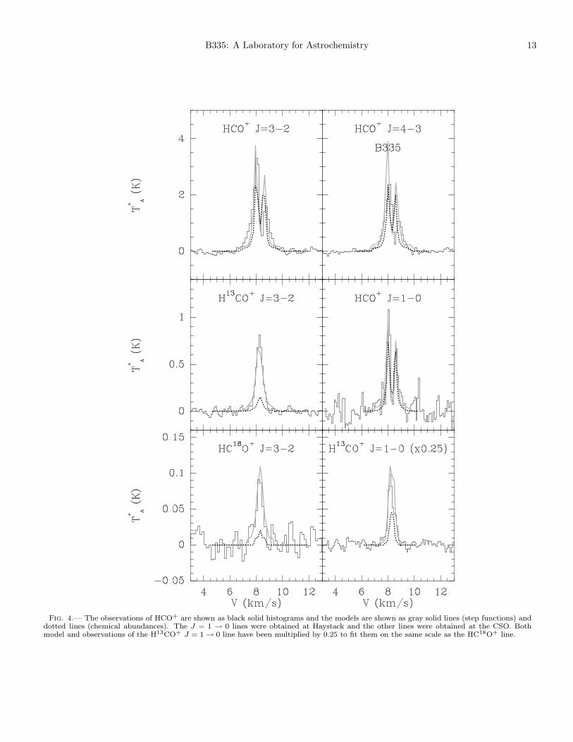
B335: A Laboratory for Astrochemistry 13
Fig. 4.— The observations of HCO+ are shown as black solid histograms and the models are shown as gray solid lines (step functions) anddotted lines (chemical abundances). The J = 1 → 0 lines were obtained at Haystack and the other lines were obtained at the CSO. Bothmodel and observations of the H13CO+
J = 1 → 0 line have been multiplied by 0.25 to fit them on the same scale as the HC18O+ line.
14 Evans et al.
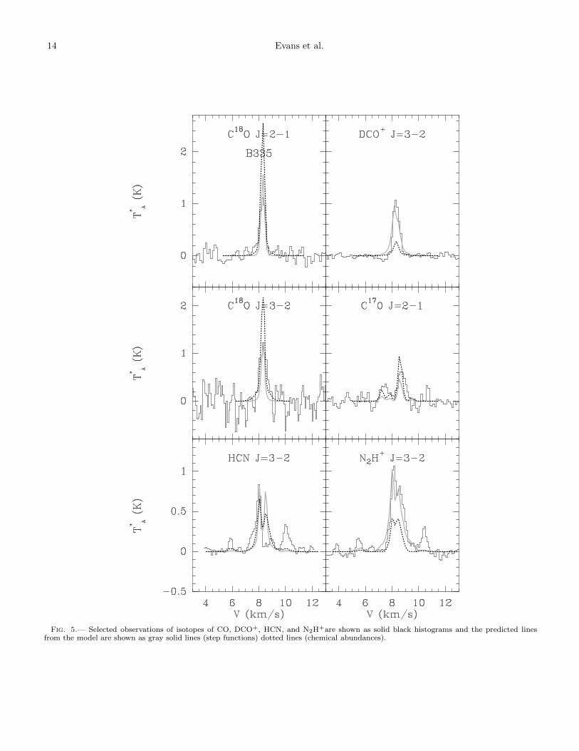
Fig. 5.— Selected observations of isotopes of CO, DCO+, HCN, and N2H+are shown as solid black histograms and the predicted linesfrom the model are shown as gray solid lines (step functions) dotted lines (chemical abundances).
B335: A Laboratory for Astrochemistry 15
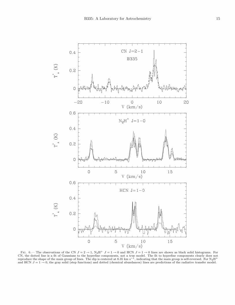
Fig. 6.— The observations of the CN J = 2 → 1, N2H+J = 1 → 0 and HCN J = 1 → 0 lines are shown as black solid histograms. For
CN, the dotted line is a fit of Gaussians to the hyperfine components, not a true model. The fit to hyperfine components clearly does notreproduce the shape of the main group of lines. The dip is centered at 8.35 km s−1, indicating that the main group is self-reversed. For N2H+
and HCN J = 1 → 0, the gray solid (step functions) and dotted (chemical abundances) lines are predictions of the radiative transfer model.
16 Evans et al.
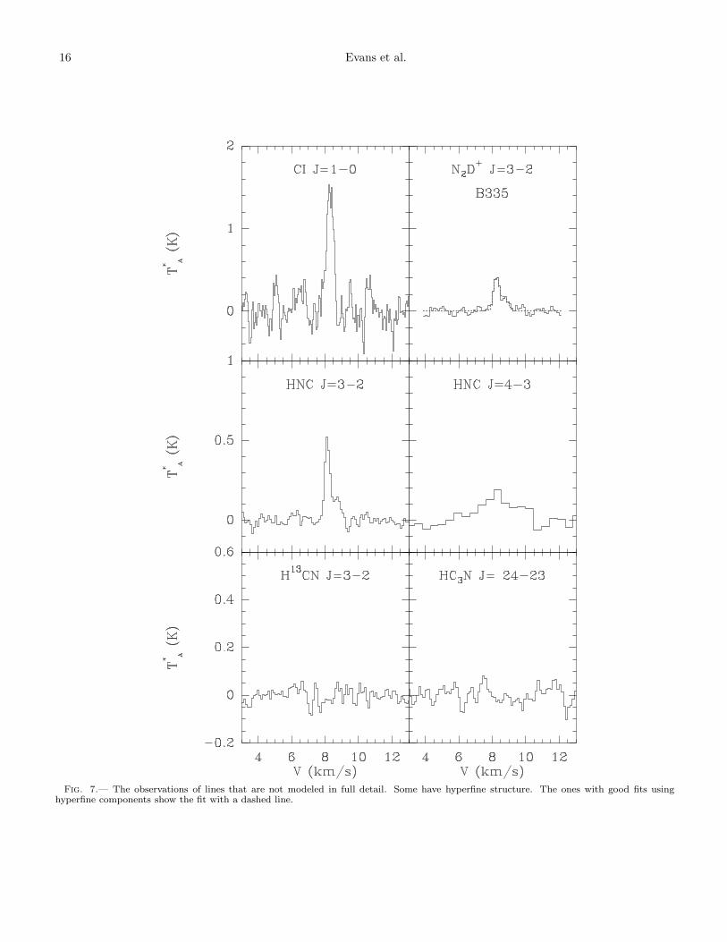
Fig. 7.— The observations of lines that are not modeled in full detail. Some have hyperfine structure. The ones with good fits usinghyperfine components show the fit with a dashed line.
B335: A Laboratory for Astrochemistry 17
-3 -2.5 -2 -1.5 -10
10
20
30
40
log r(pc)
T (
K)
3
4
5
6
Shu Model
Fig. 8.— The density and temperatures for gas and dust plotted as a function of radius for the standard model.
18 Evans et al.
Fig. 9.— The observed CS lines from Zhou et al. (1993) are plotted with the line profiles predicted by various models. The step functionmodels are gray and the evolutionary models are dotted. The bottom panel shows the best model with rinf = 0.01 pc; the second panelfrom the bottom shows the best model with rinf = 0.03 pc (same as Fig. 1); the third panel from the bottom shows the best model withrinf = 0.09 pc; and the top panel shows the best model with the rinf = 0.03 pc, but with densities enhanced by a factor of 5 everywhere, asfavored by Harvey et al. (2001).
B335: A Laboratory for Astrochemistry 19
Fig. 10.— The observed HCO+ lines are plotted on an expanded scale, with the line profiles of the best step function model (dashed)and chemical model (heavy dashed). The solid vertical line is at 8.41 km s−1, the average velocity of the dip, while the dotted vertical lineis at 8.30 km s−1, the mean velocity for optically thin lines. The shift of the dip velocity to higher velocities seen in the observations is notreproduced in the models.
20 Evans et al.
Fig. 11.— Abundance profiles. The dashed line shows the step function abundances, and the solid and dotted lines represent the abundancescalculated from the chemical evolution model of Lee et al. (2004) in the time step for rinf = 0.03 pc. In both chemical models, we used theinitial sulfur abundance greater than the standard value in Lee et al. (2004) by a factor of 5. In the chemical model with dotted lines, thecosmic-ray ionization rate is two times greater than the standard value to give the best fit to observed line profiles (Model 6 in Table 8). Thesolid line is Model 5, which uses the standard value for ionization rate.
B335: A Laboratory for Astrochemistry 21
Fig. 12.— Off-center line profiles. The gray solid (step functions) and dotted (chemical abundances) lines are predictions of the radiativetransfer model. For HCO+ and C18O, we show observed line profiles as histograms. The observations of the CS lines can be seen in Zhou etal. (1993).
22 Evans et al.
Table 1
Observing Parameters
Line ν Telescope ηmb θb δv Ref Date(GHz) (′′) (km s−1)
CI 1→0 492.1607 CSO 0.47 16 0.080 1 1996 JunCN 2→1 226.874745 CSO 0.60 27 0.14 1 1998 JulC17O 2→1 224.714368a CSO 0.81 33 0.17 1 2000 JunC18O 2→1 219.560352 CSO 0.57 28 0.15 1 1998 JulC18O 3→2 329.3305453 CSO 0.82 26 0.10 1 2000 JulHCO+ 1→0 89.188512 Haystack 0.12 25 0.10 1 1994 JunH13CO+ 1→0 86.754330 Haystack 0.12 25 0.10 1 1994 JunHCO+ 3→2 267.557619 CSO 0.65 26 0.18 1 1995 MarH13CO+ 3→2 260.255339 CSO 0.65 26 0.18 1 1995 MarHC18O+ 3→2 255.47940 CSO 0.65 26 0.18 1 1995 MarHCO+ 4→3 356.734288 CSO 0.61 20 0.14 1 1995 MarDCO+ 3→2 216.112604 CSO 0.57 28 0.16 1 1998 JulHCN 1→0 89.635847 TRAO 0.40 61 0.068 2 1997HCN 3→2 265.8864343 CSO 0.65 23 0.15 1 1996 JunH13CN 3→2 259.011814 CSO 0.65 23 0.15 1 1996 JunHNC 3→2 271.981142 CSO 0.62 22 0.11 1 1996 JunHNC 4→3 362.630303 CSO 0.53 19 1.62 1 1997 JulHC3N 24→23 218.324788 CSO 0.56 28 0.18 1 1996 JunN2H
+ 1→0 93.176258b Haystack 0.12 25 0.10 1 1994 JunN2H
+ 3→2 279.511757c CSO 0.56 22 0.12 1 1996 OctN2D
+ 3→2 231.321775 CSO 0.73 32 0.21 1 2001 Julpara-H2
13CO 101 − 000 71.02478 NRAO 0.95 89 0.206 3H2
13CO 212 − 111 137.44996 NRAO 0.72 42 0.1065 3H2CO 212 − 111 140.839518 IRAM 0.68 17 0.083 4para-H2
13CO 202 − 101 141.98375 NRAO 0.72 42 0.103 3H2
13CO 211 − 110 146.63569 NRAO 0.72 42 0.0998 3H2CO 312 − 211 225.697772 IRAM 0.50 12 0.066 4H2CO 312 − 211 225.697787 CSO 0.65 27 0.127 1 1996 Junpara-H2CO 303 − 202 218.222186 CSO 0.65 28 0.131 1 1996 JunH2CO 515 − 414 351.768645 CSO 0.53 20 0.083 1 1997 Junpara-H2CO 505 − 404 362.3530480 CSO 0.53 19 0.085 1 1997 Junpara-H2CO 523 − 422 365.3634280 CSO 0.53 19 0.085 1 1997 Jun
Note. — (a) Reference frequency for the hyperfine shifts in Ladd et al. (1998); (b) For the isolated hyperfine component (Lee et al. 2001);(c) Reference frequency for the hyperfine shifts in Caselli et al. (2002); (1) This paper; (2) Park et al. 1999; (3) Minh et al. 1995; (4) Zhou etal. 1993.
B335: A Laboratory for Astrochemistry 23
Table 2
Observational Results
Molecule Line∫
T ∗Adv T ∗
A vLSR ∆v(K km s−1) (K) (km s−1) (km s−1)
CI J = 1 → 0 0.80(0.04) 1.51(0.18) 8.29(0.01) 0.50(0.03)CNb,c J = 2 → 1 0.90(0.02) 0.43(0.02) 8.35(0.04) 0.62(0.07)C17Oa J = 2 → 1 0.46(0.07) 0.57(0.07) 8.39(0.02) 0.49(0.07)C18O J = 2 → 1 0.63(0.42) 1.10(0.10) 8.27(0.02) 0.57(0.04)C18O J = 3 → 2 0.78(0.09) 2.15(0.26) 8.33(0.04) 0.64(0.08)HCO+b J = 1 → 0 0.71(0.05) 1.15(0.11) 8.35(0.03) 0.61(0.10)H13CO+ J = 1 → 0 0.24(0.06) 0.33(0.02) 8.23(0.04) 0.58(0.03)HCO+b J = 3 → 2 3.13(0.05) 3.32(0.08) 8.46(0.04) 0.94(0.16)H13CO+ J = 3 → 2 0.46(0.01) 0.76(0.03) 8.25(0.01) 0.57(0.02)HC18O+ J = 3 → 2 0.05(0.01) 0.09(0.01) 8.26(0.04) 0.58(0.10)HCO+b J = 4 → 3 2.27(0.15) 2.35(0.06) 8.55(0.03) 0.97(0.12)DCO+ J = 3 → 2 0.78(0.03) 1.32(0.04) 8.35(0.01) 0.55(0.02)HCNb,c J = 1 → 0 0.59(0.10) 0.35(0.05) 8.39(0.01) 0.70(0.10)HCNb J = 3 → 2 0.81(0.03) 0.80(0.02) 8.40(0.20) 1.01(0.04)H13CN J = 3 → 2 · · · < 0.1 · · · · · ·HNC J = 3 → 2 0.22(0.01) 0.49(0.03) 8.16(0.01) 0.42(0.03)HNC J = 4 → 3 0.39(0.05) 0.16(0.03) 8.33(0.16) 2.3(0.4)HC3N J = 24 → 23 · · · < 0.08 · · · · · ·N2H
+d J = 1 → 0 0.13(0.01) 0.25(0.02) 8.33(0.01) 0.47(0.02)N2H
+b,c J = 3 → 2 0.95(0.08) 1.00(0.04) 8.38(0.03) 0.38(0.04)N2D
+a J = 3 → 2 0.32(0.04) 0.38(0.04) 8.36(0.02) 0.31(0.05)H2CO JK
−1K+1= 312 → 211 0.55(0.01) 0.63(0.02) 8.26(0.01) 0.82(0.02)
para-H2CO JK−1K+1
= 303 → 202 0.45(0.01) 0.59(0.03) 8.28(0.01) 0.71(0.03)H2CO JK
−1K+1= 515 → 414 0.49(0.03) 0.57(0.07) 8.30(0.02) 0.80(0.07)
para-H2CO JK−1K+1
= 505 → 404 0.40(0.06) 0.31(0.11) 8.53(0.08) 1.22(0.23)para-H2CO JK
−1K+1= 523 → 422 · · · < 0.2 · · · · · ·
Note. — (a) Hyperfine structure:∫
T∗
Adv refers to area under all lines; T∗
A refers to main peak of blended components; vLSR and ∆v are
from fit to blended components; (b) Double-peaked:∫
T ∗
Adv is for total area under both peaks; T ∗
Arefers to strongest peak; vLSR refers to
dip; ∆v is integrated intensity divided by peak T∗
A. (c) Hyperfine structure:∫
T∗
Adv refers to area under all lines; ∆v determined from isolatedhyperfine component. (d) All entries refer to the isolated hyperfine component.
Table 3
Standard Physical Model
Type a rinf rout L AV G0 ζ b ne X(CO)(km s−1) (pc) (pc) (L⊙) (mag) (s−1) (km s−1) (cm−3)
Shu 0.23 0.03 0.15 4.5 1.3 0.1 3 × 10⁻¹⁷ 0.12 1 × 10⁻³ 7.4 × 10⁻⁵
Table 4
Isotope Ratios
C/13C O/18O 18O/17O70 540 3.5
24 Evans et al.
Table 5
Aggregated Hyperfine Shiftsa and Strengthsb
C17O 2→1 HCN 1→0 HCN 3→2 N2H+ 1→0 N2H
+ 3→2∆v ri ∆v ri ∆v ri ∆v ri ∆v ri
1.157 0.040 4.849 0.333 1.749 0.037 6.936 0.037 2.015 0.0170.431 0.122 0.000 0.556 0.303 0.200 5.984 0.185 0.669 0.0150.241 0.571 −7.072 0.111 −0.030 0.725 5.545 0.111 0.416 0.084
−0.526 0.093 · · · · · · −0.611 0.001 0.956 0.185 0.266 0.094−0.926 0.016 · · · · · · −2.348 0.037 0.000 0.259 0.076 0.089−1.073 0.095 · · · · · · · · · · · · −0.611 0.111 −0.073 0.615−1.203 0.062 · · · · · · · · · · · · −8.006 0.111 −0.601 0.010
· · · · · · · · · · · · · · · · · · · · · · · · −2.644 0.011· · · · · · · · · · · · · · · · · · · · · · · · −2.773 0.014
Note. — (a) Shift in km s−1 relative to the assumed central velocity of 8.30 km s−1; (b) Relative strength (ri) normalized so that∑
ri = 1.
Table 6
Step Function Abundances
Species X(r > rinf ) X(r < rinf ) AD(Step) AD(Chem)CS 6.0 × 10⁻⁹ 6.0 × 10⁻⁹ 6.88 6.78C18O 7.4 × 10⁻⁸ 2.5 × 10⁻⁸ 3.00 3.22HCO+ 3.5 × 10⁻⁹ 3.5 × 10⁻⁸ 3.95 4.02DCO+ 6.0 × 10⁻¹¹ 6.0 × 10⁻¹⁰ 1.87 3.27N2H
+ 3.0 × 10⁻¹⁰ 3.0 × 10⁻⁹ 5.15 6.14HCN 1.0 × 10⁻⁸ 1.0 × 10⁻⁹ 5.43 4.73H2CO 7.0 × 10⁻¹⁰ 7.0 × 10⁻⁹ 2.64 3.22para-H2CO 4.0 × 10⁻¹⁰ 4.0 × 10⁻⁹ ... ...
Table 7
Variations in the Physical Model
rinf Density factor 〈AD〉a Chem Mod. 〈AD〉a
0.01 1.0 4.62 6 4.930.03 1.0 3.75 6 4.150.09 1.0 5.38 6 4.950.03 5.0 4.02 · · · · · ·
aThe mean value of AD for all species.
B335: A Laboratory for Astrochemistry 25
Table 8
Chemical Models
Model Type Dust X(S) ζ 〈AD〉a
Surface (s−1)Model 1 Step · · · · · · · · · 3.75Model 2 Chem SiO2 4 × 10⁻⁸ 3.0 × 10⁻¹⁷ 5.05Model 3 Chem CO 4 × 10⁻⁸ 3.0 × 10⁻¹⁷ 4.84Model 4 Chem H2O 4 × 10⁻⁸ 3.0 × 10⁻¹⁷ 5.89Model 5 Chem SiO2 2 × 10⁻⁷ 3.0 × 10⁻¹⁷ 4.25Model 6 Chem SiO2 2 × 10⁻⁷ 6.0 × 10⁻¹⁷ 4.15Model 7 Chem SiO2 2 × 10⁻⁷ 1.5 × 10⁻¹⁶ 4.23
aThe mean value of AD for all species.
Copyright © 2022 FDOKUMEN