Cloud Computing – CLOUD 2018 - Prof. Ravi Sandhu
420
Min Luo Liang-Jie Zhang (Eds.) 123 LNCS 10967 11th International Conference Held as Part of the Services Conference Federation, SCF 2018 Seattle, WA, USA, June 25–30, 2018 Proceedings Cloud Computing – CLOUD 2018
-
Upload
khangminh22 -
Category
Documents
-
view
4 -
download
0
Transcript of Cloud Computing – CLOUD 2018 - Prof. Ravi Sandhu

Min LuoLiang-Jie Zhang (Eds.)
123
LNCS
109
67
11th International Conference Held as Part of the Services Conference Federation, SCF 2018 Seattle, WA, USA, June 25–30, 2018 Proceedings
Cloud Computing – CLOUD 2018

Lecture Notes in Computer Science 10967
Commenced Publication in 1973Founding and Former Series Editors:Gerhard Goos, Juris Hartmanis, and Jan van Leeuwen
Editorial Board
David HutchisonLancaster University, Lancaster, UK
Takeo KanadeCarnegie Mellon University, Pittsburgh, PA, USA
Josef KittlerUniversity of Surrey, Guildford, UK
Jon M. KleinbergCornell University, Ithaca, NY, USA
Friedemann MatternETH Zurich, Zurich, Switzerland
John C. MitchellStanford University, Stanford, CA, USA
Moni NaorWeizmann Institute of Science, Rehovot, Israel
C. Pandu RanganIndian Institute of Technology Madras, Chennai, India
Bernhard SteffenTU Dortmund University, Dortmund, Germany
Demetri TerzopoulosUniversity of California, Los Angeles, CA, USA
Doug TygarUniversity of California, Berkeley, CA, USA
Gerhard WeikumMax Planck Institute for Informatics, Saarbrücken, Germany

More information about this series at http://www.springer.com/series/7409

Min Luo • Liang-Jie Zhang (Eds.)
Cloud Computing –
CLOUD 201811th International ConferenceHeld as Part of the Services Conference Federation, SCF 2018Seattle, WA, USA, June 25–30, 2018Proceedings
123

EditorsMin LuoHuawei Technologies CO., LtdShenzhenChina
Liang-Jie ZhangKingdee International Software Group CO.Ltd
ShenzhenChina
ISSN 0302-9743 ISSN 1611-3349 (electronic)Lecture Notes in Computer ScienceISBN 978-3-319-94294-0 ISBN 978-3-319-94295-7 (eBook)https://doi.org/10.1007/978-3-319-94295-7
Library of Congress Control Number: 2018947340
LNCS Sublibrary: SL3 – Information Systems and Applications, incl. Internet/Web, and HCI
© Springer International Publishing AG, part of Springer Nature 2018This work is subject to copyright. All rights are reserved by the Publisher, whether the whole or part of thematerial is concerned, specifically the rights of translation, reprinting, reuse of illustrations, recitation,broadcasting, reproduction on microfilms or in any other physical way, and transmission or informationstorage and retrieval, electronic adaptation, computer software, or by similar or dissimilar methodology nowknown or hereafter developed.The use of general descriptive names, registered names, trademarks, service marks, etc. in this publicationdoes not imply, even in the absence of a specific statement, that such names are exempt from the relevantprotective laws and regulations and therefore free for general use.The publisher, the authors, and the editors are safe to assume that the advice and information in this book arebelieved to be true and accurate at the date of publication. Neither the publisher nor the authors or the editorsgive a warranty, express or implied, with respect to the material contained herein or for any errors oromissions that may have been made. The publisher remains neutral with regard to jurisdictional claims inpublished maps and institutional affiliations.
Printed on acid-free paper
This Springer imprint is published by the registered company Springer International Publishing AGpart of Springer Nature.The registered company address is: Gewerbestrasse 11, 6330 Cham, Switzerland

Preface
This volume presents the accepted papers for the 2018 International Conference onCloud Computing (CLOUD 2018), held in Seattle, USA, during June 25–30, 2018. TheInternational Conference on Cloud Computing (CLOUD) has been a prime interna-tional forum for both researchers and industry practitioners to exchange the latestfundamental advances in the state of the art and practice of cloud computing, identifyemerging research topics, and define the future of cloud computing. All topicsregarding cloud computing align with the theme of CLOUD. We celebrated the 2018edition of the gathering by striving to advance the largest international professionalforum on cloud computing.
For this conference, each paper was reviewed by at least three independent membersof the international Program Committee. After carefully evaluating their originality andquality, we accepted 29 papers.
We are pleased to thank the authors whose submissions and participation made thisconference possible. We also want to express our thanks to the Program Committeemembers, for their dedication in helping to organize the conference and reviewing thesubmissions. We owe special thanks to the keynote speakers for their impressivespeeches. We would like to thank Chengzhong Xu, Xianghan Zheng, Dongjin Yu,Mr. Ben Goldshlag, and Pelin Angin, who provided continuous support for thisconference.
Finally, we would like to thank Rossi Kamal, Tolga Ovatman, Fadi Al-Turjman,Mohamed Nabeel Yoosuf, Bedir Tekinerdogan, and Jing Zeng for their excellent workin organizing this conference.
May 2018 Min LuoLiang-Jie Zhang

Conference Committees
General Chair
Chengzhong Xu Chinese Academy of Science (Shenzhen), China
Program Chair
Min Luo Huawei, USA
Short Paper Track Chair
Dongjin Yu Hangzhou Dianzi University, China
Publicity Chair
Pelin Angin Middle East Technical University, Turkey
Application and Industry Chair
Ben Goldshlag Goldman Sachs, USA
Program Co-chair
Xianghan Zheng Fuzhou university, China
Cloud Reliability Track Chair
Rossi Kamal Royal University of Dhaka, Bangladesh
Cloud Performance Track Chair
Tolga Ovatman Istanbul Technical University, Turkey
Cloud IoT Services Track Chair
Phu Phung University of Dayton, USA
Cloud Networking Track Chair
Fadi Al-Turjman METU Northern Cyprus Campus, Northern Cyprus

Cloud Software Engineering Track Chair
Mohammad Hammoud Carnegie Mellon University in Qatar, Qatar
Cloud Data Analytics Track Chair
Mohamed Nabeel Yoosuf Qatar Computing Research Institute, Qatar
Cloud Infrastructure and Management Track Chair
Bedir Tekinerdogan Wageningen University, The Netherlands
Services Conference Federation (SCF 2018)
General Chairs
Calton Pu Georgia Tech, USAWu Chou Vice President-Artificial Intelligence and Software
at Essenlix Corporation, USA
Program Chair
Liang-Jie Zhang Kingdee International Software Group Co., Ltd, China
Finance Chair
Min Luo Huawei, USA
Panel Chair
Stephan Reiff-Marganiec University of Leicester, UK
Tutorial Chair
Carlos A. Fonseca IBM T.J. Watson Research Center, USA
Industry Exhibit and International Affairs Chair
Zhixiong Chen Mercy College, USA
Operations Committee
Huan Chen (Chair) Kingdee Inc., ChinaJing Zeng Tsinghua University, China
VIII Conference Committees

Cheng Li Tsinghua University, ChinaYishuang Ning Tsinghua University, ChinaSheng He Tsinghua University, China
Steering Committee
Calton Pu Georgia Tech, USALiang-Jie Zhang (Chair) Kingdee International Software Group Co., Ltd., China
CLOUD 2018 Program Committee
Haopeng Chen Shanghai Jiao Tong University, ChinaSteve Crago University of Southern California, USAAlfredo Cuzzocrea University of Trieste, ItalyRoberto Di Pietro University of Rome, ItalyJ. E. (Joao Eduardo) Ferreira University of Sao Paulo, BrazilChris Gniady University of Arizona, USADaniel Grosu Wayne State University, USAWaldemar Hummer IBM T.J. Watson Research Center, USAMarty Humphrey University of Virginia, USAGueyoung Jung AT&T Labs, USANagarajan Kandasamy Drexel University, USAYasuhiko Kanemasa Fujitsu Laboratories Ltd., JapanWubin Li Ericsson Research, CanadaLi Li Essenlix Corp, USAShih-chun Lin North Carolina State University, USAJiaxiang Lin Fujian Agriculture and Forest University, ChinaLili Lin Fujian Agriculture and Forest University, ChinaXumin Liu Rochester Institute of Technology, USABrahim Medjahed University of Michigan, USANingfang Mi Northeastern University, USAShaolei Ren Florida International University, USANorbert Ritter University of Hamburg, GermanyHan Rui Chinese Academy of Sciences, ChinaRizos Sakellariou University of Manchester, BritainUpendra Sharma IBM T.J. Watson Research Center, USAJun Shen University of Wollongong, AustraliaEvgenia Smirni College of William and Mary, USAAnna Squiciarini Penn State University, USAZaogan Su Fujian Agriculture and Forest University, ChinaStefan Tai Berlin University, GermanyShu Tao IBM T. J. Watson Research Center, USAQingyang Wang Louisiana State University, USAPengcheng Xiong NEC Labs, USAYang Yang Fuzhou University, ChinaChangcai Yang Fujian Agriculture and Forest University, China
Conference Committees IX

Ayong Ye Fujian Normal University, ChinaI-Ling Yen University of Texas at Dallas, USAQi Yu Rochester Institute of Technology, USALiang-Jie Zhang Kingdee International Software Group, ChinaMing Zhao Arizona State University, USAXianghan Zheng Fuzhou University, China
X Conference Committees

Contents
Research Track: Cloud Schedule
A Vector-Scheduling Approach for Running Many-Task Applicationsin the Cloud . . . . . . . . . . . . . . . . . . . . . . . . . . . . . . . . . . . . . . . . . . . . . . 3
Brian Peterson, Yalda Fazlalizadeh, Gerald Baumgartner,and Qingyang Wang
Mitigating Multi-tenant Interference in Continuous Mobile Offloading . . . . . . 20Zhou Fang, Mulong Luo, Tong Yu, Ole J. Mengshoel,Mani B. Srivastava, and Rajesh K. Gupta
Dynamic Selecting Approach for Multi-cloud Providers . . . . . . . . . . . . . . . . 37Juliana Carvalho, Dario Vieira, and Fernando Trinta
Research Track: Cloud Data Storage
Teleporting Failed Writes with Cache Augmented Data Stores . . . . . . . . . . . 55Shahram Ghandeharizadeh, Haoyu Huang, and Hieu Nguyen
2-Hop Eclipse: A Fast Algorithm for Bandwidth-Efficient DataCenter Switching. . . . . . . . . . . . . . . . . . . . . . . . . . . . . . . . . . . . . . . . . . . 69
Liang Liu, Long Gong, Sen Yang, Jun (Jim) Xu, and Lance Fortnow
A Prediction Approach to Define Checkpoint Intervals in Spot Instances . . . . 84Jose Pergentino A. Neto, Donald M. Pianto, and Célia Ghedini Ralha
Research Track: Cloud Container
Cloud Service Brokerage and Service Arbitrage for Container-BasedCloud Services . . . . . . . . . . . . . . . . . . . . . . . . . . . . . . . . . . . . . . . . . . . . 97
Ruediger Schulze
Fault Injection and Detection for Artificial Intelligence Applicationsin Container-Based Clouds . . . . . . . . . . . . . . . . . . . . . . . . . . . . . . . . . . . . 112
Kejiang Ye, Yangyang Liu, Guoyao Xu, and Cheng-Zhong Xu
Container-VM-PM Architecture: A Novel Architecture for DockerContainer Placement . . . . . . . . . . . . . . . . . . . . . . . . . . . . . . . . . . . . . . . . 128
Rong Zhang, A-min Zhong, Bo Dong, Feng Tian, and Rui Li

Research Track: Cloud Resource Management
Renewable Energy Curtailment via Incentivized Inter-datacenterWorkload Migration . . . . . . . . . . . . . . . . . . . . . . . . . . . . . . . . . . . . . . . . 143
Ahmed Abada and Marc St-Hilaire
Pricing Cloud Resource Based on Reinforcement Learningin the Competing Environment . . . . . . . . . . . . . . . . . . . . . . . . . . . . . . . . . 158
Bing Shi, Hangxing Zhu, Han Yuan, Rongjian Shi, and Jinwen Wang
An Effective Offloading Trade-Off to Economize Energy and Performancein Edge Computing . . . . . . . . . . . . . . . . . . . . . . . . . . . . . . . . . . . . . . . . . 172
Yuting Cao, Haopeng Chen, and Zihao Zhao
Research Track: Cloud Management
Implementation and Comparative Evaluation of an Outsourcing Approachto Real-Time Network Services in Commodity Hosted Environments . . . . . . 189
Oscar Garcia, Yasushi Shinjo, and Calton Pu
Identity and Access Management for Cloud Services Usedby the Payment Card Industry . . . . . . . . . . . . . . . . . . . . . . . . . . . . . . . . . 206
Ruediger Schulze
Network Anomaly Detection and Identification Based on DeepLearning Methods . . . . . . . . . . . . . . . . . . . . . . . . . . . . . . . . . . . . . . . . . . 219
Mingyi Zhu, Kejiang Ye, and Cheng-Zhong Xu
A Feedback Prediction Model for Resource Usage and Offloading Timein Edge Computing . . . . . . . . . . . . . . . . . . . . . . . . . . . . . . . . . . . . . . . . . 235
Menghan Zheng, Yubin Zhao, Xi Zhang, Cheng-Zhong Xu,and Xiaofan Li
Application and Industry Track: Cloud Service System
cuCloud: Volunteer Computing as a Service (VCaaS) System. . . . . . . . . . . . 251Tessema M. Mengistu, Abdulrahman M. Alahmadi, Yousef Alsenani,Abdullah Albuali, and Dunren Che
CloudsStorm: An Application-Driven Framework to Enhance theProgrammability and Controllability of Cloud Virtual Infrastructures . . . . . . . 265
Huan Zhou, Yang Hu, Jinshu Su, Cees de Laat, and Zhiming Zhao
A RESTful E-Governance Application Framework for People IdentityVerification in Cloud . . . . . . . . . . . . . . . . . . . . . . . . . . . . . . . . . . . . . . . . 281
Ahmedur Rahman Shovon, Shanto Roy, Tanusree Sharma,and Md Whaiduzzaman
XII Contents

A Novel Anomaly Detection Algorithm Based on Trident Tree. . . . . . . . . . . 295Chunkai Zhang, Ao Yin, Yepeng Deng, Panbo Tian, Xuan Wang,and Lifeng Dong
Application and Industry Track: Cloud Environment Framework
Framework for Management of Multi-tenant Cloud Environments . . . . . . . . . 309Marek Beranek, Vladimir Kovar, and George Feuerlicht
Fault Tolerant VM Consolidation for Energy-Efficient Cloud Environments . . . 323Cihan Secinti and Tolga Ovatman
Over-Sampling Algorithm Based on VAE in Imbalanced Classification . . . . . 334Chunkai Zhang, Ying Zhou, Yingyang Chen, Yepeng Deng, Xuan Wang,Lifeng Dong, and Haoyu Wei
Application and Industry Track: Cloud Data Processing
A Two-Stage Data Processing Algorithm to Generate Random SamplePartitions for Big Data Analysis . . . . . . . . . . . . . . . . . . . . . . . . . . . . . . . . 347
Chenghao Wei, Salman Salloum, Tamer Z. Emara, Xiaoliang Zhang,Joshua Zhexue Huang, and Yulin He
An Improved Measurement of the Imbalanced Dataset . . . . . . . . . . . . . . . . . 365Chunkai Zhang, Ying Zhou, Yingyang Chen, Changqing Qi, Xuan Wang,and Lifeng Dong
A Big Data Analytical Approach to Cloud Intrusion Detection . . . . . . . . . . . 377Halim Görkem Gülmez, Emrah Tuncel, and Pelin Angin
Short Track
Context Sensitive Efficient Automatic Resource Schedulingfor Cloud Applications. . . . . . . . . . . . . . . . . . . . . . . . . . . . . . . . . . . . . . . 391
Lun Meng and Yao Sun
A Case Study on Benchmarking IoT Cloud Services . . . . . . . . . . . . . . . . . . 398Kevin Grünberg and Wolfram Schenck
A Comprehensive Solution for Research-Oriented Cloud Computing . . . . . . . 407Mevlut A. Demir, Weslyn Wagner, Divyaansh Dandona,and John J. Prevost
Author Index . . . . . . . . . . . . . . . . . . . . . . . . . . . . . . . . . . . . . . . . . . . . 419
Contents XIII

Research Track: Cloud Schedule

A Vector-Scheduling Approachfor Running Many-Task Applications
in the Cloud
Brian Peterson, Yalda Fazlalizadeh, Gerald Baumgartner(B),and Qingyang Wang
Division of Computer Science and Engineering, School of Electrical Engineering andComputer Science, Louisiana State University, Baton Rouge, LA 70803, USA
{brian,yalda,gb,qywang}@csc.lsu.edu
Abstract. The performance variation of cloud resources makes it dif-ficult to run certain scientific applications in the cloud because of theirunique synchronization and communication requirements. We proposea decentralized scheduling approach for many-task applications thatassigns individual tasks to cloud nodes based on periodic performancemeasurements of the cloud resources. In this paper, we present a vector-based scheduling algorithm that assigns tasks to nodes based on mea-suring the compute performance and the queue length of those nodes.Our experiments with a set of tasks in CloudLab show that the appli-cation proceeds in three distinct phases: flooding the cloud nodes withtasks, a steady state in which all nodes are busy, and the end game inwhich the remaining tasks are executed on the fastest nodes. We presentheuristics for these three phases and demonstrate with measurements inCloudLab that they result in a reduction of the overall execution timeof the many-task application.
1 Introduction
Many scientific fields require massive computational power and resources thatmight exceed those available on a single local supercomputer. Historically, therehave been two drastically different approaches for harnessing the combinedresources of a distributed collection of machines: traditional computationalsupercomputer grids and large-scale desktop-based master-worker grids. Overthe last decade, a commercial alternative has become available with cloud com-puting. For many smaller scientific applications, using cloud computing resourcesmight be cheaper than maintaining a local supercomputer.
Cloud computing has been very successful for some types of applications,especially for applications that do not require frequent communication betweendifferent cloud nodes, such as MapReduce [8] or graph-parallel [24] algorithms.However, for applications with fine-grained parallelism, such as the NAS MPIbenchmarks or atmospheric monitoring programs, it shows less than satisfac-tory performance [10,23]. The main reasons are that the performance of cloudc© Springer International Publishing AG, part of Springer Nature 2018M. Luo and L.-J. Zhang (Eds.): CLOUD 2018, LNCS 10967, pp. 3–19, 2018.https://doi.org/10.1007/978-3-319-94295-7_1
4 B. Peterson et al.
nodes is often not predictable enough, especially with virtualization, and thatthe communication latency is typically worse than that of a cluster.
For applications that can be broken into a set of smaller tasks, however,it may be possible to match the performance requirements of a task with theperformance characteristics of (a subset of) the cloud nodes. For grids and super-computers, this many-task computing approach [19] has proven very effective.E.g., Rajbhandari et al. [20] structured the computation of a quantum chemistrytensor contraction equation as a task graph with dependencies and were able toscale the computation to over 250,000 cores. They dynamically schedule taskson groups of processors and use work-stealing for load balancing.
Because of the heterogeneity resulting from virtualization, a task schedulerwould have to keep track of the performance characteristics of all cloud nodes andcommunication links. For large systems and for tasks involving fine-grained par-allelism, this would become prohibitively expensive and result in a central taskscheduler becoming a bottleneck. We, therefore, argue for the need to employ adecentralized scheduling algorithm.
IBM’s Air Traffic Control (ATC) algorithm [2] attempts to solve this problemby arranging cloud nodes in groups and by letting the leader of each group(the air traffic controller) direct the compute tasks (aircraft) from a central jobqueue to their destination worker nodes that will then execute the task. Whilethis approach distributes the load of maintaining performance information forworker nodes, the central job queue is still a potential bottleneck and the airtraffic controllers may not have enough information about the computationalrequirements and communication patterns of the individual tasks. The OrganicGrid [5,6] is a fully decentralized approach in which nodes forward tasks totheir neighbors in an overlay network. Based on performance measurements, theoverlay network is dynamically restructured to improve the overall performance.Since it was designed as a desktop grid with more heterogeneity than in the cloudand with potentially unreliable communication links, however, its algorithms areunnecessarily complex for the cloud and would result in too much overhead.
In this paper, we propose a light-weight fully decentralized approach in whichthe tasks decide on which nodes to run based on performance information adver-tised by the nodes. Similar to the Organic Grid, nodes advertise their perfor-mance to their neighbors on an overlay network and task migrate along theedges of that same overlay network. By letting the application decide whichnodes to run on, this decision can be based on knowledge about the computa-tional requirements and communication patterns that may not be available to acentralized scheduler or a system-based scheduler like the ATC algorithm.
We use a vector-based model to describe node information. By plotting thenodes in an n-dimensional space, the coefficient vector and the dot productcan be used to find the node with characteristics most similar to the vector.Therefore, it is possible to think of the vector as the direction in which workshould flow. Trivially, any scheduler should move work from a high queue lengthnode to a low queue length node. However, it may also be desirable to takeinto account a measurement of node performance, so that preference is given
A Vector-Scheduling Approach for Running Many-Task Applications 5
to run tasks on the fastest nodes. A central component of our experiments isto determine an optimal vector to minimize the time for computing jobs on adecentralized network of nodes.
The rest of this paper is organized as follows. Section 2 summarizes relateddecentralized systems and motivates our approach. In Sect. 3, we present thedesign of our vector-based task scheduling framework. Section 4 illustrates theeffectiveness of our scheduling framework using experiments. Finally, Sect. 5 dis-cusses related work and Sect. 6 concludes the paper.
2 Motivation
Prior work has shown the possibility of using a mix of decentralized strategiesfor work scheduling. The Organic Grid used a hierarchical strategy to move highperforming nodes closer to a source of work. The ATC uses controller nodesto organize groups of workers, and controllers compete to get work for theirworker nodes. We have simulated these algorithms and identified the comparativebenefits and drawbacks of each approach [17,18].
The Organic Grid’s organization helps move work to high performing nodesmore quickly, however it builds an overlay network centered around a singlework source. In a large cloud system, we may not always have a single source forwork, so we have to consider how to build a network that takes performance intoaccount when scheduling, but does not rely on a single point source of all work.We want to take the idea of measuring performance and using that informationto drive scheduling. We experimented with simulating the Organic Grid, and onetrend we noticed was that when work was added in to a new location, the overlaynetwork that was built was destroyed and recreated around the new insertionpoint. Because in the original Organic Grid, the mobile agents that reorganizedthe network were associated with individual jobs, the knowledge gained in theprevious session was lost and unavailable to the next job to use the system.
The ATC algorithm contains a degree of mid-level centralization, nodes arecategorized into worker and controllers. Controllers organize a group of work-ers, and take on groups of tasks for workers. Our simulations show that thiscan improve performance. Centralization allows the benefit of full utilization. Acontroller knows how many workers it has, and is able to pull a job that willmost completely utilize the nodes. A fully decentralized solution will not knowexactly how to make an ideally sized job at each scheduling step. However thedownside to this solution in our simulations was the communications burdenthat was placed on the controller nodes.
We choose the vector scheduling approach for our experiments, since it is fullydecentralized and lightweight, i.e., it does not have the potential communicationbottlenecks of a centralized scheduler or the ATC controller nodes and it doesnot have the high overhead of the Organic Grid.
In a decentralized network, any choice to move work has to be done basedon a limited amount of information available at a certain point in the network.We organize our experimental network as a graph of worker nodes. In our initial

6 B. Peterson et al.
Fig. 1. Average benchmark performance vs. average measured job performance forperformance and queue test
experiments, this graph is generated randomly. Each node periodically advertisesits performance and status to its neighbors on the graph. Initially, we choose thequeue length and the performance on the previous task as the information toadvertise. When a set of jobs exist at a node that node will have to make adecision based on its view of the network about whether to leave those jobs tobe completed locally or to move them to adjacent nodes in the graph.
Additionally, we need to measure the usefulness of the data we are gathering.If we measure performance, i.e., the speed at which independent tasks are com-pleted, is our measurement going to correlate to actually completing jobs morequickly? While we had several benchmarks available to us in the form of theNAS benchmark set, which has been used in prior work to test the effectivenessof cloud computing platforms [10], how relevant are these benchmarks to actualcomputing tasks? While we were not able to completely answer this questionbefore we started work, with hindsight we can measure this fairly accurately.Figure 1 shows an imperfect correlation between the job completion times andthe measured performance times from the data of specifically the Queue andPerformance mixed test that we discuss more in our experimental section. Thistest utilized the performance data to dictate where jobs were scheduled.
3 Vector-Based Job Scheduling Framework
Vector-based scheduling is the idea that there is a direction in which work shouldmove through a network of nodes. We theorize that if the nodes can be placed inan n-dimensional space based on n measurable attributes, the best direction forwork to move can be defined as a vector in that space. Therefore, we measureattributes about nodes at a given time, such as their current workload, or theirperformance on a given benchmark. After we describe each node’s position, we

A Vector-Scheduling Approach for Running Many-Task Applications 7
Table 1. Node information
Node Measured Normalized
Queue length Benchmark (sec) Queue length Benchmark (sec)
A 7 0.8 1 1
B 1 0.1 −0.71 −1
C 0 0.2 −1 −0.71
D 1 0.6 −0.71 0.43
can compare those positions to an ideal vector using the dot product operationin order to determine which nodes best fit the direction defined by that vec-tor. By collecting the dot product values of a group of nodes, we can createa weighted job distribution from any individual node to any set of neighbors.Using this methodology, we can make distributed scheduling decisions based onrecent information at any point in the network of nodes.
As an example, suppose we measure only node performance and queue length.Node A enters a redistribution cycle, as a result of having a job surplus. Itsneighbors are nodes B, C, and D. A has the information about itself and itsneighbors as seen in the left part of Table 1. E.g., A has the largest number ofjobs in the queue and it took 0.8 s for A to complete the benchmark run. Aslong as the computation cost is greater than the cost of movement, moving jobstowards idle nodes will be a good scheduling strategy We also hope to show thatmoving jobs towards higher performing nodes will be beneficial, and to whatdegree this is the case. B in this scenario is the highest performing node, and Cis the node with the fewest jobs in its queue.
We standardize the measurements to distinguish between comparatively goodcharacteristics and to evenly load the nodes. However, it can have the disadvan-tage of magnifying small differences in performance. Note that this exampleoccurs for one scheduling choice at one point in time. Therefore, we will trans-form the set {7, 1, 0, 1} into the range [-1, 1]. If another scheduling decision ismade at a later time, the existing data at that point will be transformed inde-pendently from this decision. The transformed data is shown in the right twocolumns of Table 1.
An additional factor for determining where to move jobs is the cost of move-ment. The communication cost of moving a job from one location to another mayvary from job to job depending on the memory requirements of a job. Addition-ally, in a decentralized network of independent decision makers, there is a dangerof a thrashing, where jobs are repeatedly shifted around between the same setof nodes. We have implemented two policies to mitigate this problem, althoughit may be counterproductive to completely eliminate it.
The first and simplest rule to make a decision is to provided a minimum queuelength below which a node will not attempt to move jobs. For our initial exper-iments that queue length is 1. The second possibility, which is more in line withour experimental methodology, is to provide a stasis vector as an experimental
8 B. Peterson et al.
parameter. This vector offsets the metrics of the work source node to make ita more likely candidate for work redistribution. This stasis vector is not largeenough to override a significant difference in measured node quality, but shouldbe large enough to keep insignificant changes in measured node quality fromprompting wasteful rescheduling. Proving whether a stasis vector is useful, andwhat characteristics it should have will be a focus of the experimental stage.
4 Experimental Results
4.1 Experimental Setup
Organizing our experiments has allowed us to develop a cloud experiment man-agement system. Cloud management systems, such as those used by CloudLab,have sophisticated tools to manage allocated resources. However, after resourceallocation we often end up communicating with them via ssh. Even if we deployour system in a Docker container, it is necessary to do some higher-level workto deploy the containers, perform the initial startup, and, crucially, to mutuallyidentify cloud resources to one another. A general problem, of which we onlyattack a small part, is how to make cloud resources as automatically responsiveas possible. When programming for either HPC or cloud, there are questions ofscale, appropriate resource utilization, and ideal levels of parallelization, whichmight completely or at least approximately be automatically solvable, but stillquite often they need to be configured in a tedious and manual manner. Also ide-ally, we want cloud resources to be as transparent as possible, but this requiresintelligence to automatically allocate and schedule as much work as possible.
Building an experiment also requires describing the network that will exe-cute the developing work. Although we consider a decentralized system that willbe applicable to very large scale networks, we are somewhat restricted to theactual hardware available in our labs or on CloudLab. Therefore, most of theexperiments concern how we can schedule work on heterogeneous decentralizednetworks, and what measurements and approaches produce measurably usefulresults. We can characterize a set of interconnected computing resources as aconnected graph, but to determine what characteristics that graph should pos-sess, we use the Erdos-Renyi algorithm for graph generation [9]. We define aprobability that any two nodes in the graph of computing platforms are con-nected, and generate different graphs for different experiments. We examine anygenerated graph and ensure that it is connected by adding extra links betweenlow ranked vertices of disconnected portions.
To perform our experiment, we first allocate machines and then start Dockercontainers on each machine. One container functions as an experimental con-troller, while the rest are experimental nodes. The controller is started first andis provided with information that defines the experiment. It knows how manynodes will participate in the experiment, how long the experiment should take,and what configuration information to give to the experimental nodes. The con-troller builds the graph that defines node-neighbor relationships, and contains
A Vector-Scheduling Approach for Running Many-Task Applications 9
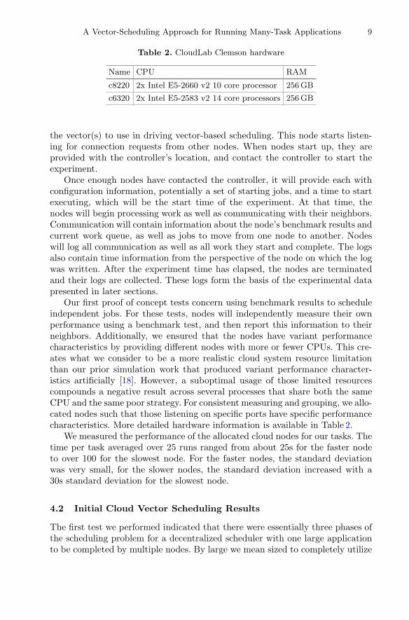
Table 2. CloudLab Clemson hardware
Name CPU RAM
c8220 2x Intel E5-2660 v2 10 core processor 256GB
c6320 2x Intel E5-2583 v2 14 core processors 256GB
the vector(s) to use in driving vector-based scheduling. This node starts listen-ing for connection requests from other nodes. When nodes start up, they areprovided with the controller’s location, and contact the controller to start theexperiment.
Once enough nodes have contacted the controller, it will provide each withconfiguration information, potentially a set of starting jobs, and a time to startexecuting, which will be the start time of the experiment. At that time, thenodes will begin processing work as well as communicating with their neighbors.Communication will contain information about the node’s benchmark results andcurrent work queue, as well as jobs to move from one node to another. Nodeswill log all communication as well as all work they start and complete. The logsalso contain time information from the perspective of the node on which the logwas written. After the experiment time has elapsed, the nodes are terminatedand their logs are collected. These logs form the basis of the experimental datapresented in later sections.
Our first proof of concept tests concern using benchmark results to scheduleindependent jobs. For these tests, nodes will independently measure their ownperformance using a benchmark test, and then report this information to theirneighbors. Additionally, we ensured that the nodes have variant performancecharacteristics by providing different nodes with more or fewer CPUs. This cre-ates what we consider to be a more realistic cloud system resource limitationthan our prior simulation work that produced variant performance character-istics artificially [18]. However, a suboptimal usage of those limited resourcescompounds a negative result across several processes that share both the sameCPU and the same poor strategy. For consistent measuring and grouping, we allo-cated nodes such that those listening on specific ports have specific performancecharacteristics. More detailed hardware information is available in Table 2.
We measured the performance of the allocated cloud nodes for our tasks. Thetime per task averaged over 25 runs ranged from about 25s for the faster nodeto over 100 for the slowest node. For the faster nodes, the standard deviationwas very small, for the slower nodes, the standard deviation increased with a30s standard deviation for the slowest node.
4.2 Initial Cloud Vector Scheduling Results
The first test we performed indicated that there were essentially three phases ofthe scheduling problem for a decentralized scheduler with one large applicationto be completed by multiple nodes. By large we mean sized to completely utilize
10 B. Peterson et al.
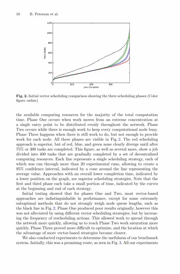
Fig. 2. Initial vector scheduling comparison showing the three scheduling phases (Colorfigure online)
the available computing resources for the majority of the total computationtime. Phase One occurs when work moves from an extreme concentration ata single entry point to be distributed evenly throughout the network. PhaseTwo occurs while there is enough work to keep every computational node busy.Phase Three happens when there is still work to do, but not enough to providework for each node. All three phases are visible in Fig. 2. The red schedulingapproach is superior, but of red, blue, and green none clearly diverge until after75% or 300 tasks are completed. This figure, as well as several more, show a jobdivided into 400 tasks that are gradually completed by a set of decentralizedcomputing resources. Each line represents a single scheduling strategy, each ofwhich was run through more than 20 experimental runs, allowing to create a95% confidence interval, indicated by a cone around the line representing theaverage value. Approaches with an overall lower completion time, indicated bya lower position on the graph, are superior scheduling strategies. Note that thefirst and third phase each take a small portion of time, indicated by the curvesat the beginning and end of each strategy.
Initial testing showed that for phases One and Two, most vector-basedapproaches are indistinguishable in performance, except for some extremelysuboptimal methods that do not strongly weigh node queue lengths, such asthe black line in Fig. 2. Phase One produced poor results originally, however thiswas not alleviated by using different vector scheduling strategies, but by increas-ing the frequency of rescheduling actions. This allowed work to spread throughthe network more quickly, allowing us to reach Phase Two work saturation morequickly. Phase Three proved more difficult to optimize, and the location at whichthe advantage of more vector-based strategies became clearer.
We also conducted experiments to determine the usefulness of our benchmarksystem. Initially, this was a promising route, as seen in Fig. 3. All our experiments
A Vector-Scheduling Approach for Running Many-Task Applications 11
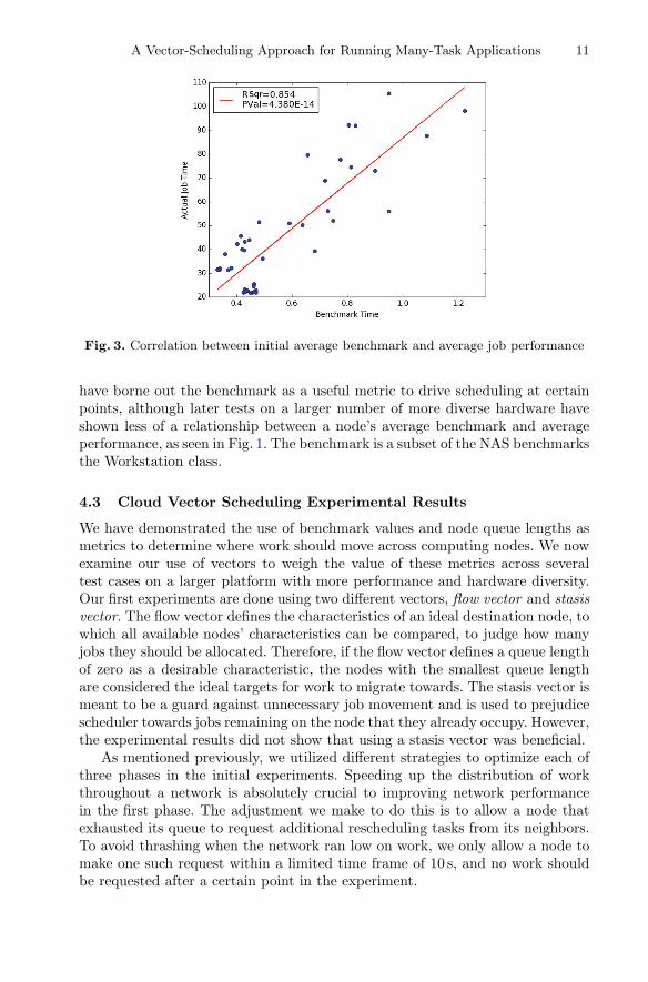
Fig. 3. Correlation between initial average benchmark and average job performance
have borne out the benchmark as a useful metric to drive scheduling at certainpoints, although later tests on a larger number of more diverse hardware haveshown less of a relationship between a node’s average benchmark and averageperformance, as seen in Fig. 1. The benchmark is a subset of the NAS benchmarksthe Workstation class.
4.3 Cloud Vector Scheduling Experimental Results
We have demonstrated the use of benchmark values and node queue lengths asmetrics to determine where work should move across computing nodes. We nowexamine our use of vectors to weigh the value of these metrics across severaltest cases on a larger platform with more performance and hardware diversity.Our first experiments are done using two different vectors, flow vector and stasisvector. The flow vector defines the characteristics of an ideal destination node, towhich all available nodes’ characteristics can be compared, to judge how manyjobs they should be allocated. Therefore, if the flow vector defines a queue lengthof zero as a desirable characteristic, the nodes with the smallest queue lengthare considered the ideal targets for work to migrate towards. The stasis vector ismeant to be a guard against unnecessary job movement and is used to prejudicescheduler towards jobs remaining on the node that they already occupy. However,the experimental results did not show that using a stasis vector was beneficial.
As mentioned previously, we utilized different strategies to optimize each ofthree phases in the initial experiments. Speeding up the distribution of workthroughout a network is absolutely crucial to improving network performancein the first phase. The adjustment we make to do this is to allow a node thatexhausted its queue to request additional rescheduling tasks from its neighbors.To avoid thrashing when the network ran low on work, we only allow a node tomake one such request within a limited time frame of 10 s, and no work shouldbe requested after a certain point in the experiment.
12 B. Peterson et al.
While this achieves the desired result of improved initial performance, theoverall performance of the network suffers. Even though we attempt to avoidflooding the network with rescheduling requests at the end, the additional taxon the resources of the poor performers causes their last one or two jobs to takeas much as three times as long as their already slower completion times. Recallthat poor performance in this context is caused by sharing a CPU, therefore, apoor choice for a scheduling strategy on multiple nodes sharing the same CPUhave a strong negative influence on the performance of each individual node.We argue that this is a valuable artifact of this experimental system, as sharedresources are a potential problem with low-cost cloud systems. We eliminatethis problem by creating a simpler strategy that only allows rapid reschedulingoperations in response to the introduction of new work into the system.
The final phase of the network, when there is no longer enough work tosatisfy every node in the system, requires a different approach. In our initialexperiments, we had two goals. First, work must be moved away from low per-forming nodes and onto higher performing nodes. Second, any other burden onthe network while the last jobs are completed should be avoided. Accomplishingthe second goal involves turning off the functionality that allows nodes to requestwork once the initial job set has spread throughout the network. In these exper-iments we simply turned off the functionality after a certain amount of time inearly Phase Two to stop allowing nodes to request more work. For future workhowever, we will look at a more sophisticated way to make this choice.
Flow-vector-based scheduling was most beneficial in optimizing the finalphase. For most of the duration of an experiment, any rescheduling based onrelative queue length is more or less indistinguishable. As long as it does notimpose a large computational burden it will spread work throughout the net-work, saturating the available computational resources. However, just beforesome nodes become idle, it is important to move work preferentially to highperforming nodes, so that the last few straggling jobs are given to nodes thatwill complete the jobs faster. To do this we change from a flow vector of (−1.0,−0.3), which prefers a shorter queue, and considers a better performance lessrelevant, to a vector of (−0.7, −0.5), which puts more emphasis on performance.
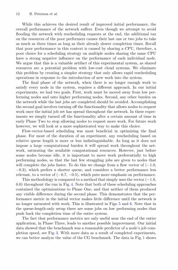
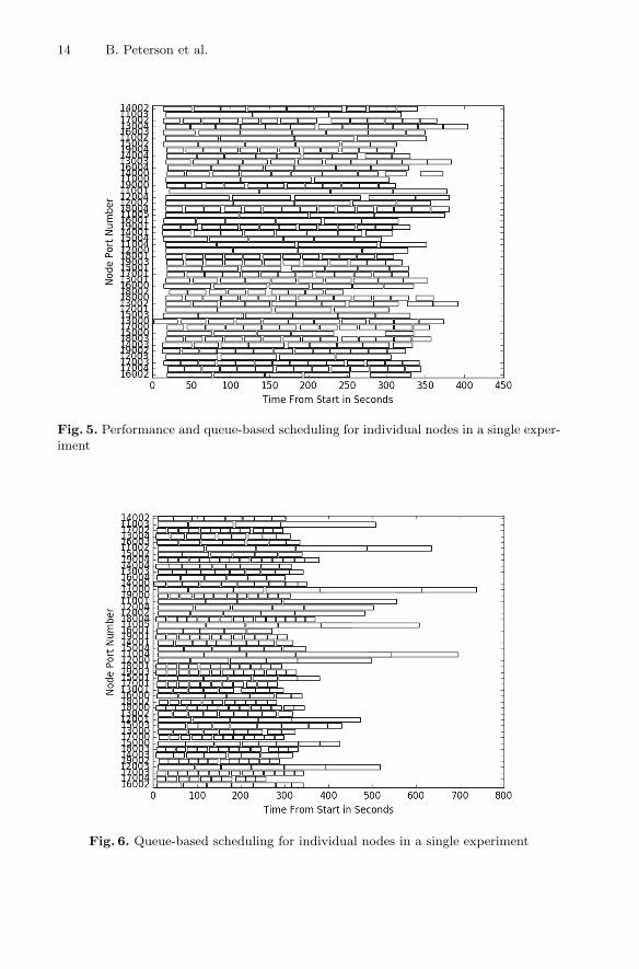
This methodology is compared to a method that simply uses the vector (−1.0,0.0) throughout the run in Fig. 4. Note that both of these scheduling approachescontained the optimizations to Phase One, and that neither of them producedany visible difference during the second phase. This demonstrates that the per-formance metric in the initial vector makes little difference until the network isno longer saturated with work. This is illustrated in Figs. 5 and 6. Note that inthe queue-length-only setup there are some jobs on low performing nodes thatpush back the completion time of the entire system.
The fact that performance metrics are only useful near the end of the entireapplication, in Phase Three, leads to another possible improvement. Our initialdata showed that the benchmark was a reasonable predictor of a node’s job com-pletion speed, see Fig. 3. With more data as a result of completed experiments,we can better analyze the value of the CG benchmark. The data in Fig. 1 shows

A Vector-Scheduling Approach for Running Many-Task Applications 13
Fig. 4. Job completion time comparison between balanced queue and performance-based scheduling (blue) and queue-based scheduling (red) (Color figure online)
a much weaker relationship between average benchmark and average perfor-mance. Regardless, experimental results have shown the most recent benchmarkto be useful when driving scheduling decisions as seen in Fig. 4. Additionally,this data shows the relationship between the average benchmark performancemeasurement, and the average job completion time. The relationship is not asconsistent on the more diverse hardware used for the larger scale tests as it wason the original smaller scale setup. The measurement that is used for schedul-ing is not the overall average benchmark measurement but the most recent onethat a node has taken. This distinction is valuable, because we suggest the mostrecently taken benchmark most accurately measures the node’s expected per-formance at that time, considering that other usage of the node’s hardware is alikely cause of performance degradation.
Note that in Fig. 1 the group that is spread along the x-axis (benchmark val-ues), but are all consistently low on the y-axis (actual job performance). Thesemeasurements are all from nodes with a port in the 13000 s. The 13000 range isone of the subsets meant to be high performers, which was born out by the actualjob completion rates, but not by the average benchmark measurements. Nodesin a given port range are executed on a subset of the hardware with similarcharacteristics, which are meant to provide either advantages or disadvantagesin performance. The error bars in this figure are simply one standard devia-tion, indicating that the nodes with worse performance also had more highlydeviating performance. We use standard deviation here, as opposed to a 95%confidence interval, as we are more interested in seeing the result of the perfor-mance modifications on the experiments that were run, and less interested indrawing conclusions about them as samples from a larger population.
Even if the average benchmark value is not useful, the most recent perfor-mance measure may be, as it did produce the more advantageous experimental
14 B. Peterson et al.
Fig. 5. Performance and queue-based scheduling for individual nodes in a single exper-iment
Fig. 6. Queue-based scheduling for individual nodes in a single experiment

A Vector-Scheduling Approach for Running Many-Task Applications 15
results presented originally in Fig. 4. As a result of both the deficiencies in bench-mark selection, and the result that a performance measurement is only usefulnear the end of work scheduling, a more simple and obvious methodology canbe implemented for problems whose tasks are of consistent or predictable sizes.We considered using historical data at the beginning of the project, but initiallyrejected the approach because we would need some stop-gap measure to utilizebefore historical data was generated. A benchmark-based methodology seemedto be a better general solution, and may still be applicable given more relevantbenchmarks. However, given that more than half of the work can be completedbefore implementing performance based scheduling, we can utilize the partialhistorical data available when some work has been completed to drive perfor-mance based scheduling, instead of using a benchmark. This result is shown inFig. 7. The final phase curve is even less evident in these results, indicating thatthis strategy is superior.
Fig. 7. Historical performance-based scheduling comparison
5 Related Work
Research on traditional grid scheduling has focused on algorithms for determin-ing an optimal computation schedule based on the assumption that sufficientlydetailed and up-to-date knowledge of the systems state is available to a singleentity (the metascheduler) [1,11,21]. While this approach results in a very effi-cient utilization of the resources, it does not scale to large numbers of machines,since maintaining a global view of the system becomes prohibitively expensive.Variations in resource availability and potentially unreliable networks might evenmake it impossible.

16 B. Peterson et al.
A number of large-scale desktop grid systems have been based on variants ofthe master/workers model [4,7,14,16]. The fact that SETI@home had scaled toover 5 million nodes and that some of these systems have resulted in commer-cial enterprises shows the level of technical maturity reached by the technology.However, the obtainable computing power is constrained by the performance ofthe master, especially for data-intensive applications. Since networks cannot beassumed to be reliable, large desktop grids are designed for independent taskapplications with relatively long-running individual tasks.
Cloud computing has been very successful for several types of applications,especially for applications that do not require frequent communication betweendifferent cloud nodes, such as MapReduce [8] or graph-parallel [24] algorithms.However, for applications with fine-grained parallelism, such as the NAS MPIbenchmarks or atmospheric monitoring programs, it shows less than satisfac-tory performance [10,23]. The main reasons are that the performance of cloudnodes is often not predictable enough, especially with virtualization, and thatthe communication latency is typically worse than that of a cluster [23]. Whileit is possible to rent dedicated clusters from cloud providers, they are signifi-cantly more expensive per compute hour than virtual machines (VMs). Withvirtualization, however, the user may not know whether a pair of VMs run onthe same physical machine, are in the same rack, or are on different ends of thewarehouse.
A related problem is the management of resources in a data center. Tsoet al. [22] survey resource management strategies for data centers. Luo et al. [15]and Gutierrez-Estevez and Luo [12] propose a fine-grained centralized resourcescheduler that takes application needs into consideration. By contrast, our app-roach uses existing VMs, measures their performance and lets the applicationdecide which tasks to run on which nodes. However, it is not clear that a cen-tralized scheduler would be fine-grained enough for large many-task and high-performance computing applications without creating a bottleneck.
6 Conclusion
We have proposed a decentralized scheduling approach for many-task applica-tions that assigns individual tasks to cloud nodes in order to achieve both fast jobexecution time and high resource efficiency. We have presented a vector-basedscheduling algorithm that assigns tasks to nodes based on measuring the com-pute performance and the queue length of those nodes. Our experiments witha set of tasks in CloudLab show that by applying our vector-based schedulingalgorithm the application proceeds in three distinct phases: flooding the cloudnodes with tasks, a steady state in which all nodes are busy, and the final phasein which the remaining tasks are executed on the fastest nodes. We have alsopresented heuristics for these three phases and have demonstrated with mea-surements in CloudLab that they result in a reduction of the overall executiontime of the many-task application. Our measurements have shown that initiallyit is more important to use queue-length as a metric to flood all the nodes, whilein the last phase performance becomes a more important metric.

A Vector-Scheduling Approach for Running Many-Task Applications 17
The disadvantage of a decentralized scheduling approach is that it does notguarantee perfect resource utilization, as shown by the gaps in Fig. 5. The mainadvantage, however, is that there is no central scheduler that could become acommunication bottleneck.
The goal of this work is to allow large-scale many-task applications to be exe-cuted efficiently in the cloud. The measurements we have presented represent thefirst step toward this goal. For future work, we plan to use quantum chemistrysimulations as a target application [3,13]. Using the approach from Rajbhan-dari et al. [20], this will involve scheduling a task graph with individual tasksof varying size, many of which requiring multiple nodes for a distributed tensorcontraction. For good performance, it is critical that all nodes participating ina distributed contraction (or matrix multiplication) have similar performancecharacteristics and communication latency between them. This will require peri-odically running measurement probes that test the performance of each node, thecommunication latency with neighbors, and possibly other values. For our vectorscheduling approach, we will then add communication latency as an additionaldimension and allow scheduling a single task on a group of nodes with similarperformance and low latency between them. A task graph with dependencies willlikely result in more than three distinct phases and, therefore, require differentheuristics.
Fine-tuning the performance of such applications in the cloud will requirefinding the best structure of the overlay network (probably based on perfor-mance measurements instead of being randomly generated), finding the mosteffective measurement probes and measurement frequency, and running large-scale experiments.
Acknowledgment. This research was partially supported by CloudLab (NSF Award#1419199), by the National Science Foundation under grant CNS-1566443, and by theLouisiana Board of Regents under grant LEQSF(2015-18)-RD-A-11.
References
1. Abramson, D., Giddy, J., Kotler, L.: High performance parametric modeling withNimrod/G: killer application for the global grid? In: Proceedings of InternationalParallel and Distributed Processing Symposium, pp. 520–528, May 2000
2. Barsness, E., Darrington, D., Lucas, R., Santosuosso, J.: Distributed job schedulingin a multi-nodal environment. US Patent 8,645,745, 4 February 2014. http://www.google.com/patents/US8645745
3. Baumgartner, G., Auer, A., Bernholdt, D., Bibireata, A., Choppella, V., Cociorva,D., Gao, X., Harrison, R., Hirata, S., Amoorthy, S.K., Krishnan, S., Lam, C.,Lu, Q., Nooijen, M., Pitzer, R., Ramanujam, J., Sadayappan, P., Sibiryakov, A.:Synthesis of high-performance parallel programs for a class of AB initio quantumchemistry models. Proc. IEEE 93(2), 276–292 (2005)
4. Buaklee, D., Tracy, G., Vernon, M.K., Wright, S.: Near-optimal adaptive controlof a large Grid application. In: Proceedings of International Conference on Super-computing, pp. 315–326, June 2002
18 B. Peterson et al.
5. Chakravarti, A.J., Baumgartner, G., Lauria, M.: The Organic Grid: self-organizingcomputation on a peer-to-peer network. IEEE Trans. Syst. Man Cybern. Part A35(3), 373–384 (2005)
6. Chakravarti, A.J., Baumgartner, G., Lauria, M.: Self-organizing scheduling on theOrganic Grid. Intl. J. High-Perf. Comput. Appl. 20(1), 115–130 (2006)
7. Chien, A.A., Calder, B., Elbert, S., Bhatia, K.: Entropia: architecture and perfor-mance of an enterprise desktop grid system. J. Parallel Distrib. Comput. 63(5),597–610 (2003)
8. Dean, J., Ghemawat, S.: MapReduce: simplified data processing on large clusters.Commun. ACM 51(1), 107–113 (2008)
9. Erdos, P., Renyi, A.: On the evolution of random graphs. Publ. Math. Inst. Hung.Acad. Sci 5(1), 17–60 (1960)
10. Evangelinos, C., Hill, C.N.: Cloud computing for parallel scientific HPC applica-tions: feasibility of running coupled atmosphere-ocean climate models on Amazon’sEC2. In: 1st Workshop on Cloud Computing and its Applications (CCA) (2008)
11. Grimshaw, A.S., Wulf, W.A.: The Legion vision of a worldwide virtual computer.Commun. ACM 40(1), 39–45 (1997)
12. Gutierrez-Estevez, D.M., Luo, M.: Multi-resource schedulable unit for adaptiveapplication-driven unified resource management in data centers. In: 2015 Inter-national Telecommunication Networks and Applications Conference (ITNAC),November 2015
13. Hartono, A., Lu, Q., Henretty, T., Krishnamoorthy, S., Zhang, H., Baumgartner,G., Bernholdt, D.E., Nooijen, M., Pitzer, R.M., Ramanujam, J., Sadayappan, P.:Performance optimization of tensor contraction expressions for many-body meth-ods in quantum chemistry. J. Phys. Chem. 113(45), 12715–12723 (2009)
14. Litzkow, M., Livny, M., Mutka, M.: Condor – a hunter of idle workstations. In: Pro-ceedings of the 8th International Conference of Distributed Computing Systems,pp. 104–111, June 1988
15. Luo, M., Li, L., Chou, W.: ADARM: an application-driven adaptive resource man-agement framework for data centers. In: 2017 IEEE International Conference onAI and Mobile Services (AIMS), June 2017
16. Maheswaran, M., Ali, S., Siegel, H.J., Hensgen, D.A., Freund, R.F.: Dynamicmatching and scheduling of a class of independent tasks onto heterogeneous com-puting systems. In: Proceedings of the 8th Heterogeneous Computing Workshop,pp. 30–44, April 1999
17. Peterson, B.: Decentralized scheduling for many-task applications in the hybridcloud. Ph.D. thesis, Louisiana State University, Baton Rouge, LA, May 2017
18. Peterson, B., Baumgartner, G., Wang, Q.: A decentralized scheduling frameworkfor many-task scientific computing in a hybrid cloud. Serv. Trans. Cloud Comput.5(1), 1–13 (2017)
19. Raicu, I., Foster, I.T., Zhao, Y.: Many-task computing for grids and supercomput-ers. In: Proceedings of the 2008 Workshop on Many-Task Computing on Grids andSupercomputers (MTAGS 2008), Austin, TX, pp. 1–11. IEEE November 2008
20. Rajbhandari, S., Nikam, A., Lai, P.W., Stock, K., Krishnamoorthy, S., Sadayap-pan, P.: A communication-optimal framework for contracting distributed tensors.In: Proceedings of SC 2014, the International Conference on High PerformanceComputing, Networking, Storage, and Analysis, New Orleans, LA, 16–21 Novem-ber 2014 (2014)
21. Taylor, I., Shields, M., Wang, I.: 1 - resource management of Triana P2P services.In: Nabrzyski, J., Schopf, J.M., Weglarz, J. (eds.) Grid Resource Management.Springer, Boston (2003)
A Vector-Scheduling Approach for Running Many-Task Applications 19
22. Tso, F.P., Jouet, S., Pezaros, D.P.: Network and server resource managementstrategies for data centre infrastructures: a survey. Comput. Netw. 106(4), 209–225(2016)
23. Walker, E.: Benchmarking Amazon EC2 for high-performance scientific computing.In: LOGIN, vol. 33, no. 5, pp. 18–23 (2008)
24. Xin, R.S., Gonzalez, J.E., Franklin, M.J., Stoica, I.: GraphX: a resilient distributedgraph system on Spark. In: First International Workshop on Graph Data Man-agement Experiences and Systems, GRADES 2013, pp. 2:1–2:6. ACM, New York(2013)

Mitigating Multi-tenant Interferencein Continuous Mobile Offloading
Zhou Fang1(B), Mulong Luo2, Tong Yu3, Ole J. Mengshoel3,Mani B. Srivastava4, and Rajesh K. Gupta1
1 University of California San Diego, San Diego, [email protected]
2 Cornell University, Ithaca, USA3 Carnegie Mellon University, Pittsburgh, USA
4 University of California, Los Angeles, Los Angeles, USA
Abstract. Offloading computation to resource-rich servers is effectivein improving application performance on resource constrained mobiledevices. Despite a rich body of research on mobile offloading frame-works, most previous works are evaluated in a single-tenant setting,i.e., a server is assigned to a single client. In this paper we considerthat multiple clients offload various continuous mobile sensing appli-cations with end-to-end delay constraints, to a cluster of machines asthe server. Contention for shared computing resources on a server canunfortunately result in delays and application malfunctions. We presenta two-phase Plan-Schedule approach to mitigate multi-tenant resourcecontention, thus to reduce offloading delays. The planning phase pre-dicts future workloads from all clients, estimates contention, and devisesoffloading schedule to remove or reduce contention. The scheduling phasedispatches arriving offloaded workloads to the server machine that min-imizes contention, according to the running workloads on each machine.We implement the methods into ATOMS (Accurate Timing predictionand Offloading for Mobile Systems), a framework that adopts predic-tion of workload computing times, estimation of network delays, andmobile-server clock synchronization techniques. Using several mobilevision applications, we evaluate ATOMS under diverse configurationsand prove its effectiveness.
1 Introduction
Problem Background: Recent advances in mobile computing have made manyinteresting vision and cognition applications feasible. For example, cognitiveassistance [1] and augmented reality [2] applications process continuous streamsof image data to provide new capabilities on mobile platforms. However, advancesin computing power on embedded devices do not satisfy such growing needs. Toextend mobile devices with richer computing resources, offloading computationto remote servers has been introduced [1,3–5]. The servers can be either deployedin low-latency and high-bandwidth local clusters that provide timely offloadingc© Springer International Publishing AG, part of Springer Nature 2018M. Luo and L.-J. Zhang (Eds.): CLOUD 2018, LNCS 10967, pp. 20–36, 2018.https://doi.org/10.1007/978-3-319-94295-7_2
Mitigating Multi-tenant Interference in Continuous Mobile Offloading 21
running
t_send t_recv
Server
Clientnew t_send
queueing
data new data result
t_server t_start
t_end
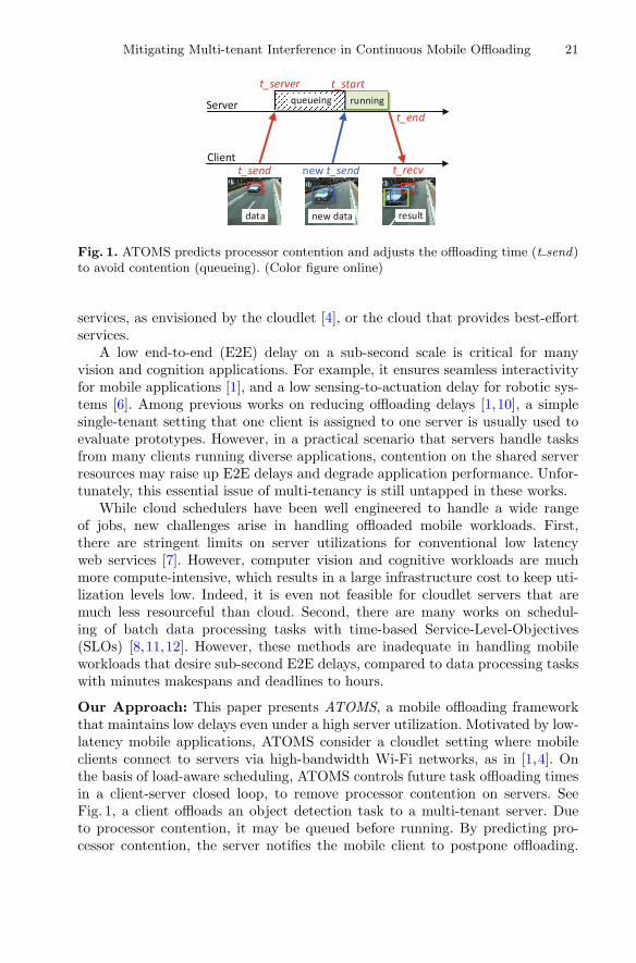
Fig. 1. ATOMS predicts processor contention and adjusts the offloading time (t send)to avoid contention (queueing). (Color figure online)
services, as envisioned by the cloudlet [4], or the cloud that provides best-effortservices.
A low end-to-end (E2E) delay on a sub-second scale is critical for manyvision and cognition applications. For example, it ensures seamless interactivityfor mobile applications [1], and a low sensing-to-actuation delay for robotic sys-tems [6]. Among previous works on reducing offloading delays [1,10], a simplesingle-tenant setting that one client is assigned to one server is usually used toevaluate prototypes. However, in a practical scenario that servers handle tasksfrom many clients running diverse applications, contention on the shared serverresources may raise up E2E delays and degrade application performance. Unfor-tunately, this essential issue of multi-tenancy is still untapped in these works.
While cloud schedulers have been well engineered to handle a wide rangeof jobs, new challenges arise in handling offloaded mobile workloads. First,there are stringent limits on server utilizations for conventional low latencyweb services [7]. However, computer vision and cognitive workloads are muchmore compute-intensive, which results in a large infrastructure cost to keep uti-lization levels low. Indeed, it is even not feasible for cloudlet servers that aremuch less resourceful than cloud. Second, there are many works on schedul-ing of batch data processing tasks with time-based Service-Level-Objectives(SLOs) [8,11,12]. However, these methods are inadequate in handling mobileworkloads that desire sub-second E2E delays, compared to data processing taskswith minutes makespans and deadlines to hours.
Our Approach: This paper presents ATOMS, a mobile offloading frameworkthat maintains low delays even under a high server utilization. Motivated by low-latency mobile applications, ATOMS consider a cloudlet setting where mobileclients connect to servers via high-bandwidth Wi-Fi networks, as in [1,4]. Onthe basis of load-aware scheduling, ATOMS controls future task offloading timesin a client-server closed loop, to remove processor contention on servers. SeeFig. 1, a client offloads an object detection task to a multi-tenant server. Dueto processor contention, it may be queued before running. By predicting pro-cessor contention, the server notifies the mobile client to postpone offloading.
22 Z. Fang et al.
0 10 20 30Time (s)
0
1
2
3
4
Load
0
2
4
6
8
Cor
es
(a) Processor Contention
0 10 20 30Time (s)
0
1
2
3
4
Load
0
2
4
6
8
Cor
es
(b) ATOMS
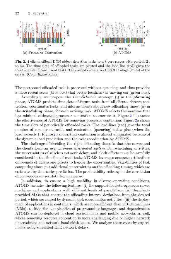
Fig. 2. 4 clients offload DNN object detection tasks to a 8-core server with periods 2 sto 5 s. The time slots of offloaded tasks are plotted and the load line (red) gives thetotal number of concurrent tasks. The dashed curve gives the CPU usage (cores) of theserver. (Color figure online)
The postponed offloaded task is processed without queueing, and thus providesa more recent scene (blue box) that better localizes the moving car (green box).
Accordingly, we propose the Plan-Schedule strategy: (i) in the planningphase, ATOMS predicts time slots of future tasks from all clients, detects con-tention, coordinates tasks, and informs clients about new offloading times; (ii) inthe scheduling phase, for each arriving task, ATOMS selects the machine thathas minimal estimated processor contention to execute it. Figure 2 illustratesthe effectiveness of ATOMS for removing processor contention. Figure 2a showsthe time slots of periodically offloaded tasks. The load lines (red) give the totalnumber of concurrent tasks, and contention (queueing) takes place when theload exceeds 1. Figure 2b shows that contention is almost eliminated because ofthe dynamic load prediction and the task coordination by ATOMS.
The challenge of deciding the right offloading times is that the server andthe clients form an asynchronous distributed system. For scheduling activities,the uncertainties of wireless network delays and clock offsets must be carefullyconsidered in the timeline of each task. ATOMS leverages accurate estimationson bounds of delays and offsets to handle the uncertainties. Variabilities of taskcomputing times put additional uncertainties on the offloading timing, which areestimated by time series prediction. The predictability relies upon the correlationof continuous sensor data from cameras.
In addition, to ensure a high usability in diverse operating conditions,ATOMS includes the following features: (i) the support for heterogeneous servermachines and applications with different levels of parallelism; (ii) the client-provided SLOs that control the offloading interval deviations from the desiredperiod, which are caused by dynamic task coordination activities; (iii) the deploy-ment of applications in containers, which are more efficient than virtual machines(VMs), to hide the complexities of programming languages and dependencies.ATOMS can be deployed in cloud environments and mobile networks as well,where removing resource contention is more challenging due to higher networkuncertainties and network bandwidth issues. We analyze these cases by experi-ments using simulated LTE network delays.

Mitigating Multi-tenant Interference in Continuous Mobile Offloading 23
This paper makes three contributions: (i) a novel Plan-Schedule scheme thatcoordinates future offloaded tasks to remove resource contention, on top of load-aware scheduling; (ii) a framework that accurately estimates and controls thetiming of offloading tasks through computing time prediction, network latencyestimation and clock synchronization; and (iii) methods to predict processorusage and detect multi-tenant contention on distributed container-based servers.
The rest of this paper is organized as follows. We discuss the related workin Sect. 2, and describe the applications and the performance metrics in Sect. 3.In Sect. 4 we explain the offloading workflow and the plan-schedule algorithms.Then we detail the system implementations in Sect. 5. Experimental results areanalyzed in Sect. 6. In Sect. 7 we summarize this paper.
2 Related Work
Mobile Offloading: Many previous works are on reducing E2E delays in mobileoffloading frameworks [1,9,10]. Gabriel [1] deploys cognitive engines in a nearbycloudlet that is only one wireless hop away to minimize network delays. Time-card [9] controls the user-perceived delays by adapting server-side processingtimes, based on measured upstream delays and estimated downstream delays.Glimpse [10] hides network delays of continuous object detection tasks by track-ing objects on the mobile side, based on stale results from the server. This paperstudies the fundamental issue of resource contention on multi-tenant mobileoffloading servers, however, not yet considered by the previous works.
Cloud Schedulers: Workload scheduling in cloud computing has already beenintensely studied. These systems leverage rich information, for example, esti-mates and measurements on resource demands and running times, to reserveand allocate resources, and reorder tasks in queue [8,11,12]. Because data pro-cessing tasks have much larger time scales of makespan and deadline, usuallyranging from minutes to hours, these methods are inadequate in handling real-time mobile offloading tasks that desires sub-second delays.
Real-Time Schedulers: Real-time (RT) schedulers in [13–15] are designed forlow latency and periodical tasks on multi-processor systems. However, theseschedulers do not work in the scenario of mobile offloading. First, the RT sched-ulers can not handle network delays and uncertainties. Second, the RT schedulersare designed to minimize deadline miss rates, whereas our goal is to minimizeE2E delays. In addition, the RT schedulers use worst-case computing times inscheduling. It results in an undesired low utilization for applications with highlyvarying computing times. As a novel approach for the mobile scenarios, ATOMSmakes dynamic predictions and coordinations for incoming offloaded tasks, usingestimated task computing times and network delays.
24 Z. Fang et al.
3 Mobile Workloads
3.1 Applications
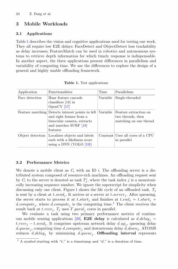
Table 1 describes the vision and cognitive applications used for testing our work.They all require low E2E delays: FaceDetect and ObjectDetect lose trackabilityas delay increases; FeatureMatch can be used in robotics and autonomous sys-tems to retrieve depth information for which timely response is indispensable.In another aspect, the three applications present differences in parallelism andvariability of computing time. We use the differences to explore the design of ageneral and highly usable offloading framework.
Table 1. Test applications
Application Functionalities Time Parallelism
Face detection Haar feature cascadeclassifiers [16] inOpenCV [17]
Variable Single-threaded
Feature matching Detects interest points in leftand right frames from abinocular camera, extractsand matches SURF [18]features
Variable Feature extraction ontwo threads, thenmatching on one thread
Object detection Localizes objects and labelseach with a likeliness scoreusing a DNN (YOLO [19])
Constant Uses all cores of a CPUin parallel
3.2 Performance Metrics
We denote a mobile client as Ci with an ID i. The offloading server is a dis-tributed system composed of resource-rich machines. An offloading request sentby Ci to the server is denoted as task T i
j , where the task index j is a monotoni-cally increasing sequence number. We ignore the superscript for simplicity whendiscussing only one client. Figure 1 shows the life cycle of an offloaded task. Tj
is sent by a client at t sendj . It arrives at a server at t serverj . After queueing,the server starts to process it at t startj and finishes at t endj = t startj +d computej , where d computej is the computing time.1 The client receives theresult back at t recvj . Tj uses T paralj cores in parallel.
We evaluate a task using two primary performance metrics of continu-ous mobile sensing applications [20]. E2E delay is calculated as d delayj =t recvj − t sendj . It comprises upstream network delay d upj , queueing delayd queuej , computing time d computej and downstream delay d downj . ATOMSreduces d delayj by minimizing d queuej . Offloading interval represents
1 A symbol starting with “t ” is a timestamp and “d ” is a duration of time.

Mitigating Multi-tenant Interference in Continuous Mobile Offloading 25
the time span between successive offloaded tasks of a client, calculated asd intervalj = t sendj − t sendj−1. Clients offload tasks periodically and arefree to adjust offloading periods. Applications can thus tune offloading periodfor energy consumption and performance trade-off. Ideally any interval is equalto d periodi, the current period of client Ci. In ATOMS, however, the inter-val becomes non-constant due to task coordination. We desire stable sens-ing and offloading activities, so smaller interval jitters are preferred, given byd jitterij = d intervalij − d periodi.
4 Framework Design
As shown in Fig. 3, ATOMS is composed of one master server and multipleworker servers. The master communicates with clients and dispatches tasks toworkers for execution. It is responsible for planning and scheduling tasks.
Master
Scheduler
Workers
Compu ngEngines
Client
App
Client Heap
PlannerReserva on queues
Fig. 3. The architecture of the ATOMS framework.
4.1 Worker and Computing Engine
We first describe how to deploy applications on workers. A worker machinehosts one or more computing engines. Each computing engine runs an offload-ing application encapsulated in a container. Our implementation adopts Dockercontainers.2 We use Docker’s resource APIs to set processor share, limit andaffinity, as well as memory limit for each container. We focus on CPUs as thecomputing resource in this paper. The total number of CPU cores of worker Wk
is W cpuk. The support for GPUs lies in our future work.A worker can have multiple engines for the same application in order to
fully exploit multi-core CPUs, or host different types of engines to share themachine by multiple applications. In this case, the total workloads of all engineson a worker may exceed the limit of processor resource (W cpu). Accordingly,2 Docker: https://www.docker.com/.
26 Z. Fang et al.
FaceDetect
Engine2:FeatureMatch
Engine0:FaceDetect
Engine1:FaceDetect
me
Load
1
2
3
IncomingFeatureMatch
Conten on
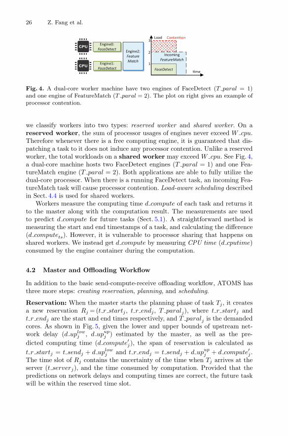
Fig. 4. A dual-core worker machine have two engines of FaceDetect (T paral = 1)and one engine of FeatureMatch (T paral = 2). The plot on right gives an example ofprocessor contention.
we classify workers into two types: reserved worker and shared worker. On areserved worker, the sum of processor usages of engines never exceed W cpu.Therefore whenever there is a free computing engine, it is guaranteed that dis-patching a task to it does not induce any processor contention. Unlike a reservedworker, the total workloads on a shared worker may exceed W cpu. See Fig. 4,a dual-core machine hosts two FaceDetect engines (T paral = 1) and one Fea-tureMatch engine (T paral = 2). Both applications are able to fully utilize thedual-core processor. When there is a running FaceDetect task, an incoming Fea-tureMatch task will cause processor contention. Load-aware scheduling describedin Sect. 4.4 is used for shared workers.
Workers measure the computing time d compute of each task and returns itto the master along with the computation result. The measurements are usedto predict d compute for future tasks (Sect. 5.1). A straightforward method ismeasuring the start and end timestamps of a task, and calculating the difference(d computets). However, it is vulnerable to processor sharing that happens onshared workers. We instead get d compute by measuring CPU time (d cputime)consumed by the engine container during the computation.
4.2 Master and Offloading Workflow
In addition to the basic send-compute-receive offloading workflow, ATOMS hasthree more steps: creating reservation, planning, and scheduling.
Reservation: When the master starts the planning phase of task Tj , it createsa new reservation Rj = (t r startj , t r endj , T paralj), where t r startj andt r endj are the start and end times respectively, and T paralj is the demandedcores. As shown in Fig. 5, given the lower and upper bounds of upstream net-work delay (d uplowj , d upupj ) estimated by the master, as well as the pre-dicted computing time (d compute′
j), the span of reservation is calculated ast r startj = t sendj + d uplowj and t r endj = t sendj + d upupj + d compute′
j .The time slot of Rj contains the uncertainty of the time when Tj arrives at theserver (t serverj), and the time consumed by computation. Provided that thepredictions on network delays and computing times are correct, the future taskwill be within the reserved time slot.

Mitigating Multi-tenant Interference in Continuous Mobile Offloading 27
compu ng
t_send
Server
Client
uncertaintyt_r_start t_r_end
d_uplow
d_upup
Fig. 5. Processor reservation for a future offloaded task includes the uncertainty ofarriving time at the server and its computing time.
Planning: The planning phase runs before the real offloading. It coordinatesfuture tasks of all clients to ensure that the total amount of all reservations neverexceeds the limit of total processor resources of all workers. Client Ci registersat the master to initialize the offloading process. The master assigns it a futuretimestamp t send0 indicating when to send the first task. The master creates areservation for task Tj and plans it when tnow = t r startj − d future wheretnow is the master’s current clock time, and d future is a parameter for how farafter tnow that the planning phase covers. The planner predicts and coordinatesfuture tasks that start before tnow + d future.
T inext is the next task of client Ci to plan. The master plans future tasks
in ascending order of start time t r startinext. For a new task to be plannedwith the earliest t r startinext, the planner creates a new reservation Ri
next. Theplanner takes Rnext as input. It detects resource contention, and reduces thatby adjusting the sending times of both the new task and a few planned tasks.We defer the details of planning to Sect. 4.3. d informi is a parameter of Ci forhow early the master should inform the client about the adjusted task sendingtime. A reservation Ri
j remains adjustable until tnow = t sendij - d informi.
The planner then removes Rj and notifies the client. Upon receiving t sendj ,the client sets a timer to offload Tj .
Scheduling: The client offloads Tj to the master when the timer at t sendjtimeouts. After receiving the task, using the information of currently runningtasks on each worker, the scheduler selects the worker that induces the leastprocessor contention. The master dispatches it to the worker and gets back theresult. We give the details in Sect. 4.4.
4.3 Planning Algorithms
The planning algorithm decides the adjustments to sending times of future tasksfrom each client. An optimal algorithm minimizes jitters of offloading intervals,while ensuring that the total processor usage is within the limit, and SLOs onoffloading intervals are satisfied. Instead of solving this complex optimizationproblem numerically, we adopt a heuristic and feedback-control approach thatadjusts future tasks in a fixed window from tnow +d inform to tnow +d future.Our approach is able to improve the accuracy of computing time prediction by

28 Z. Fang et al.
using a small predicting window (see Sect. 5.1), and naturally handle changes ofclient number and periods.
The planner buffers reservations in reservation queues. A reservation queuestands for a portion of processor resource in the cluster. A queue Qk has aresource limit Q cpuk with cores as the unit, used for contention detection. Thesum of Q cpu of all queues is equal to the total cores in the cluster. Each com-puting engine is assigned to a reservation queue. The parallelism of a reservationT paral is determined by the processor limit of computing engines. For example,T paral of a fine-parallelized task is different for an engine on a dual-core worker(T paral = 2) and one on a quad-core worker (T paral = 4).
Contention Detection: When the planner receives a new reservation Rnew, itfirst selects a queue to place it in. It iterates over all queues, for Qk, calculatesthe needed amount of time (Δ) to adjust Rnew, and the total processor usage(Θk) of Qk during the time slot of Rnew. The planner selects the queue withthe minimal Δ. In doing so, it checks whether the total load on Qk after addingRnew exceeds the limit Q cpu. If so, the algorithm calculates Δ: the contentioncan be eliminated after postponing Rnew by Δ. Otherwise Δ = 0. We give anexample in Fig. 6 that a new reservation R2
0 is being inserted into a queue. Theblack line in the lower plot is the total load. Contention arises after adding R2
0.It can be removed by postponing R2
0 to the end time of R11. Δ is thus obtained.
Fig. 6. An example of detecting processor contention and calculating required reser-vation adjustment. The top plot shows a reservation queue and the bottom plot showsthe calculated total load load(t).
If two or more planning queues have the same Δ, e.g., several queues arecontention-free (Δ = 0), the planner calculates the processor usage Θ duringthe time slot of Rnew: Θ =
∫ t r endnew
t r startnewload(t)dt. We consider two strategies.
The Best-Fit strategy selects Q that has the highest Θ, which packs reservationsas tightly as possible and leaves the least margin of processor resources on thequeue. The other strategy is Worst-Fit that, in contrast, selects the queue withthe lowest Θ. We study their difference through evaluations in Sect. 6.3.

Mitigating Multi-tenant Interference in Continuous Mobile Offloading 29
SLOs: In the next coordination step, rather than simply postponing Rnew byΔ, the planner moves ahead a few planned reservations as well, to reduce theduration to postpone Rnew. The coordination process takes Δ as input andadjusts reservations according to cost (R cost), a metric on how far the measuredoffloading interval d interval deviates from the client’s SLOs (a list of desiredpercentiles of d interval). For example, a client with period 1 s may require alower bound d slo10% > 0.9 s and an upper bound d slo90% < 1.1 s.
The master calculates R cost when it plans a new task, using the mea-sured percentiles of interval (d intervalp). For the new reservation (Rnew) tobe postponed, the cost R cost+ is obtained from the upper bounds: R cost+ =max(maxp∈∪+(d intervalp − d slop), 0) where p is a percentile and ∪+ is theset of percentiles that have upper bounds in the SLOs. R cost+ is the maximalinterval deviation from the SLOs. For tasks to be moved ahead, deviation fromlower bounds (∪−) are used instead to get the cost R cost−. The cost is a weightbetween two clients to decide the adjustment on each. SLOs with tight boundson d interval make the client less affected during the coordination process.
4.4 Scheduling Algorithms
The ATOMS scheduler dispatches tasks arriving at the master to the most suit-able worker machine that minimizes processor contention. The scheduler keepsa global FIFO task queue for buffer tasks when all computing engines are busy.For each shared worker, there is a local FIFO queue for each application that itserves. When a task arrives, the scheduler first searches for available computingengines on any reserved workers. It dispatches the task if one is found and thescheduling process ends. If there is no reserved worker, or no engine is free, thescheduler checks shared workers that are able to run the application. It selectsthe best worker based on processor contention Φ and usage Θ. The task is thendispatched to a free engine on the selected shared worker. If no engine is free onthe worker, the task is put into the worker’s local task queue.
Here we detail the policy to select a shared worker. The scheduler uses esti-mated end time t end′ of all running tasks on each worker, obtained by predictedcomputing time d compute′. To schedule Tnew, it calculates the load load(t) oneach worker using t end′, including Tnew. The resource contention Φk on workerWk is calculated by Φk =
∫ t end′new
tnowmax(load(t) − W cpuk, 0)dt. The worker
with the smallest Φ is selected to run Tnew. For workers with identical Φ, similarto the planning algorithm, we use processor usage Θ as the selection metric. Wecompare the two selection methods, Best-Fit and Worst-Fit, through evaluationsin Sect. 6.
5 Implementation
In this section we present the implementation of computing time prediction,network delay estimation and clock synchronization.

30 Z. Fang et al.
5.1 Prediction on Computing Time
Accurate prediction of computing time is essential for resource reservation.Underestimation leads to failure in detecting resource contention, and overes-timation causes larger interval jitters. We use upper bound estimation for appli-cations with a low variability of computing times, and time series prediction forapplications with a high variability. Given that Tn is the last completed taskof client Ci, instead of just predicting Tn+1 (the next task to run), ATOMSneeds to predict Tnext (the next task to plan, next > n). Npredict = next - ngives how many values it needs to predict since the last sample. It is decidedby the parameter d future (Sect. 4.2) and the period of the client, calculated as�d future/d periodi�.
Upper Bound Estimation. The first method estimates the upper boundof samples using a TCP retransmission timeout estimation algorithm [21]. Wedenote the value to predict as y. The estimator keeps a smoothed estimationys ← (1 − α) · ys + α · yi.) and a variation yvar ← (1 − β) · yvar + β · |ys − yi|.The upper bound yup is given by yup = ys + κ · yvar, where α, β and κ areparameters. This method outputs yup as the prediction of d compute for Tnext.This lightweight method is adequate for applications with low computing timevariability, such as ObjectDetect. It tends to overestimate for applications withhighly varying computing times because it uses upper bound as the prediction.
Time Series Linear Regression. In the autoregressive model for time seriesprediction problems, the value yn at index n is assumed to be a weightedsum of previous samples in a moving window with size k. That is, yn =b + w1yn−1 + · · · + wkyn−k + εn, where yn−i is the ith sample before the nth,wi is the corresponding coefficient and εn is the noise term. We use this modelto predict yn. The inputs (yn−1 to yn−k) are the previous k samples measuredby workers. We use a recursive approach to predict the Npredictth sample afteryn−1: to predict yi+1, the predicted yi is used as the last sample. This approachis flexible to predict arbitrary future samples, however, as Npredict increases, theaccuracy degrades because the prediction error is accumulated. The predictorkeeps a model for each client which is trained either online or offline.
5.2 Estimation on Upstream Latency
As discussed in Sect. 4.2, because network delays dup may have large fluctuations,we use the lower and upper bounds (d uplow, d upup) instead of the exact valuein the reservation. The TCP retransmission timeout estimator [21] described inSect. 5.1 is used to estimate network delay bounds. We use subtraction insteadof addition to obtain the lower bound. The estimator has a non-zero error whena new sample of dup falls out of the bounds, calculated as its deviation from thenearest bound. The error is positive if dup exceeds d upup, and negative if it issmaller than d uplow. The estimation uncertainty is given by d upup - d uplow.

Mitigating Multi-tenant Interference in Continuous Mobile Offloading 31
Because the uncertainty is included in task reservation, a larger uncertaintyoverclaims the reservation time slot, which causes higher interval jitters andlower processor utilizations.
We measure dup of offloading 640×480 frames with sizes from 21 KB to 64 KB,using Wi-Fi networks. To explore networks with higher delays and uncertain-ties, we obtain simulated delays of Verizon LTE networks using the Mahimahitool [22]. The CDFs of network latencies are plotted in Fig. 7a. We demonstratethe estimator performance (error and uncertainty) in Fig. 7b. Results show thatthe estimation uncertainty for Wi-Fi networks is small, and it is very large forLTE (maximal value is 2.6 s). We demonstrate how errors and uncertaintiesinfluence offloading performance through experiments in Sect. 6.
0 200 400 600 800 1000Upstream Latency (ms)
0
0.2
0.4
0.6
0.8
1
CD
F
Wi-FiLTE
(a) Upstream latency.
-500 0 500 1000Duration (ms)
0
0.2
0.4
0.6
0.8
1
CD
F
Wi-FiuncertaintyLTEuncertaintyWi-Fi errorLTE error
(b) Uncertainty and error.
Fig. 7. Upstream latency of Wi-Fi and LTE networks, with uncertainty and error ofestimation. The maximal latency is 1.1 s for Wi-Fi and 3.2 s for LTE. The parametersof estimator are α = 0.125, β = 0.125, κ = 1.
5.3 Clock Synchronization
We seek a general solution for clock synchronization without patching the OSof mobile clients. The ATOMS master is synchronized to the global time usingNTP. Because time service now is ubiquitous on mobile devices, we require clientsto be coarsely synchronized to the global time. We do fine clock synchronizationas follows. Client sends out a NTP synchronization request to the master eachtime it receives an offloading result to avoid the wake-up delay [9]. To eliminatethe influence of packet delay spikes, the client buffers Nntp responses and runsa modified NTP algorithm [23]. It applies clock filter, selection, clustering andcombining algorithms to Nntp responses and outputs a robust estimate on clockoffset. It also outputs the bounds of the offset. ATOMS uses the clock offset tosynchronize timestamps between clients and the master, and uses the bounds inall timestamp calculations to consider the remaining clock uncertainties.
6 Evaluation
6.1 Experiment Setup
Baselines: We compare ATOMS with baseline schedulers to prove its effec-tiveness for improving offloading performance. The baseline schedulers use
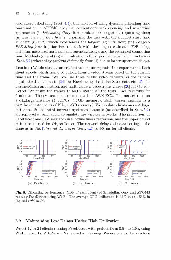
32 Z. Fang et al.
load-aware scheduling (Sect. 4.4), but instead of using dynamic offloading timecoordination in ATOMS, they use conventional task queueing and reorderingapproaches: (i) Scheduling Only : it minimizes the longest task queueing time;(ii) Earliest-start-time-first : it prioritizes the task with the smallest start timeat client (t send), which experiences the longest lag until now; (iii) Longest-E2E-delay-first : it prioritizes the task with the longest estimated E2E delay,including measured upstream and queueing delays, and the estimated computingtime. Methods (ii) and (iii) are evaluated in the experiments using LTE networks(Sect. 6.2) where they perform differently from (i) due to larger upstream delays.
Testbed: We simulate a camera feed to conduct reproducible experiments. Eachclient selects which frame to offload from a video stream based on the currenttime and the frame rate. We use three public video datasets as the camerainput: the Jiku datasets [24] for FaceDetect; the UrbanScan datasets [25] forFeatureMatch application, and multi-camera pedestrians videos [26] for Object-Detect. We resize the frames to 640 × 480 in all the tests. Each test runs for5 minutes. The evaluations are conducted on AWS EC2. The master runs ona c4.xlarge instance (4 vCPUs, 7.5 GB memory). Each worker machine is ac4.2xlarge instance (8 vCPUs, 15 GB memory). We emulate clients on c4.2xlargeinstances. Pre-collected network upstream latencies (as described in Sect. 5.2)are replayed at each client to emulate the wireless networks. The prediction forFaceDetect and FeatureMatch uses offline linear regression, and the upper boundestimator is used for ObjectDetect. The network delay estimator setting is thesame as in Fig. 7. We set d inform (Sect. 4.2) to 300 ms for all clients.
400 600 800 1000Interval (ms)
0
0.2
0.4
0.6
0.8
1
CD
F Sched OnlyATOMS
0 200 400 600 800 1000Delay (ms)
0
0.2
0.4
0.6
0.8
1
CD
F
Sched OnlyATOMS
(a) 12 clients.
400 600 800 1000Interval (ms)
0
0.2
0.4
0.6
0.8
1
CD
F Sched OnlyATOMS
0 200 400 600 800 1000Delay (ms)
0
0.2
0.4
0.6
0.8
1
CD
F
Sched OnlyATOMS
(b) 18 clients.
400 600 800 1000Interval (ms)
0
0.2
0.4
0.6
0.8
1
CD
F Sched OnlyATOMS
0 200 400 600 800 1000Delay (ms)
0
0.2
0.4
0.6
0.8
1
CD
F
Sched OnlyATOMS
(c) 24 clients.
Fig. 8. Offloading performance (CDF of each client) of Scheduling Only and ATOMSrunning FaceDetect using Wi-Fi. The average CPU utilization is 37% in (a), 56% in(b) and 82% in (c).
6.2 Maintaining Low Delays Under High Utilization
We set 12 to 24 clients running FaceDetect with periods from 0.5 s to 1.0 s, usingWi-Fi networks. d future = 2 s is used in planning. We use one worker machine
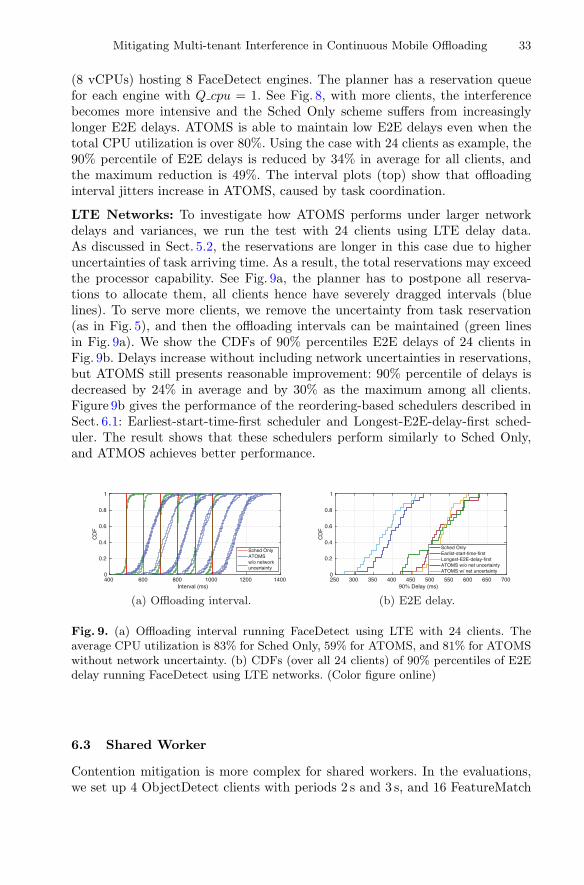
Mitigating Multi-tenant Interference in Continuous Mobile Offloading 33
(8 vCPUs) hosting 8 FaceDetect engines. The planner has a reservation queuefor each engine with Q cpu = 1. See Fig. 8, with more clients, the interferencebecomes more intensive and the Sched Only scheme suffers from increasinglylonger E2E delays. ATOMS is able to maintain low E2E delays even when thetotal CPU utilization is over 80%. Using the case with 24 clients as example, the90% percentile of E2E delays is reduced by 34% in average for all clients, andthe maximum reduction is 49%. The interval plots (top) show that offloadinginterval jitters increase in ATOMS, caused by task coordination.
LTE Networks: To investigate how ATOMS performs under larger networkdelays and variances, we run the test with 24 clients using LTE delay data.As discussed in Sect. 5.2, the reservations are longer in this case due to higheruncertainties of task arriving time. As a result, the total reservations may exceedthe processor capability. See Fig. 9a, the planner has to postpone all reserva-tions to allocate them, all clients hence have severely dragged intervals (bluelines). To serve more clients, we remove the uncertainty from task reservation(as in Fig. 5), and then the offloading intervals can be maintained (green linesin Fig. 9a). We show the CDFs of 90% percentiles E2E delays of 24 clients inFig. 9b. Delays increase without including network uncertainties in reservations,but ATOMS still presents reasonable improvement: 90% percentile of delays isdecreased by 24% in average and by 30% as the maximum among all clients.Figure 9b gives the performance of the reordering-based schedulers described inSect. 6.1: Earliest-start-time-first scheduler and Longest-E2E-delay-first sched-uler. The result shows that these schedulers perform similarly to Sched Only,and ATMOS achieves better performance.
400 600 800 1000 1200 1400Interval (ms)
0
0.2
0.4
0.6
0.8
1
CD
F
Sched OnlyATOMSw/o networkuncertainty
(a) Offloading interval.
250 300 350 400 450 500 550 600 650 70090% Delay (ms)
0
0.2
0.4
0.6
0.8
1
CD
F
Sched OnlyEarlist-start-time-firstLongest-E2E-delay-firstATOMS w/o net uncertaintyATOMS w/ net uncertainty
(b) E2E delay.
Fig. 9. (a) Offloading interval running FaceDetect using LTE with 24 clients. Theaverage CPU utilization is 83% for Sched Only, 59% for ATOMS, and 81% for ATOMSwithout network uncertainty. (b) CDFs (over all 24 clients) of 90% percentiles of E2Edelay running FaceDetect using LTE networks. (Color figure online)
6.3 Shared Worker
Contention mitigation is more complex for shared workers. In the evaluations,we set up 4 ObjectDetect clients with periods 2 s and 3 s, and 16 FeatureMatch

34 Z. Fang et al.
clients with periods 2 s, 2.5 s, 3 s and 3.5 s. d future = 6 s is used in the planner.We use 4 shared workers (c4.2xlarge), and each hosts 4 FeatureMatch enginesand 1 ObjectDetect engine.
Planning Schemes: We compare three schemes of planning: (i) a global reser-vation queue (Q cpu = 32) is used for 4 workers; (ii) 4 reservation queues(Q cpu = 8) are used and Best-Fit is used to select queue; (iii) 4 queues areused with Worst-Fit selection. Load-aware scheduling with Worst-Fit workerselection is used. The CDFs of interval (top) and E2E delay (bottom) of allclients are given in Fig. 10. It shows that Worst-Fit adjusts tasks more aggres-sively and causes the largest interval jitter. It allocates FeatureMatch tasks (lowparallelism) more evenly to all reservation queues. Resource contention is morelikely to take place when ObjectDetect (high parallelism) is planned, so moreadjustments are made. The advantage of Worst-Fit is the improved delay per-formance. See the delay plots in Fig. 10, Worst-Fit evidently performs better forthe 4 ObjectDetect clients: the worst E2E delay of the 4 clients is 786 ms forWorst-Fit, 1111 ms for Best-Fit and 1136 ms for Global. The delay performanceof FeatureMatch is similar for the three schemes.
2000 2500 3000Interval (ms)
0
0.2
0.4
0.6
0.8
1
CD
F
P=GlobalP=Best-FitP=Worst-Fit
ObjectDetect
2000 2500 3000 3500Interval (ms)
0
0.2
0.4
0.6
0.8
1
CD
F P=GlobalP=Best-FitP=Worst-Fit
FeatureMatch
400 600 800 1000 1200Delay (ms)
0
0.2
0.4
0.6
0.8
1
CD
F
P=GlobalP=Best-FitP=Worst-Fit
ObjectDetect
200 400 600 800 1000 1200 1400Delay (ms)
0
0.2
0.4
0.6
0.8
1
CD
F
P=GlobalP=Best-FitP=Worst-Fit
FeatureMatch
Fig. 10. Interval and E2E delay of 4 ObjectDetect and 16 FeatureMatch clients, usingdifferent planning schemes. The average CPU utilization is 36%.
Scheduling Schemes: Figure 11 shows the E2E delays using different schedul-ing schemes: (i) a simple scheduler that selects the first available engine; (ii)a load-aware scheduler with Best-Fit worker usage selection; (iii) a load-awarescheduler with Worst-Fit selection. The planner uses 4 reservation queues withWorst-Fit selection. For the simple scheduling, ObjectDetect tasks that can beparallelized on all 8 cores are more likely to be influenced by contention. Fea-tureMatch requires 2 cores at most and can get enough processors more easily.Best-Fit performs the best for ObjectDetect, whereas it degrades dramaticallyfor FeatureMatch clients. The reason is that the scheduler tries to pack incoming

Mitigating Multi-tenant Interference in Continuous Mobile Offloading 35
tasks as tightly as possible on workers. As a consequence, it leaves enough spaceto schedule highly parallel ObjectDetect tasks. However, due to the errors ofcomputing time prediction and network estimation, there is a higher possibilityof contention for the tightly placed FeatureMatch tasks. The Worst-Fit methodhas the best performance for FeatureMatch tasks and still maintains reasonablylow delays for ObjectDetect. Therefore it is the most suitable approach in thiscase. Figure 12 compares the 90% E2E delay of all clients between SchedulingOnly and ATOMS (Worst-Fit scheduling). In average, ATOMS reduces the 90%percentile E2E delay by 49% for the ObjectDetect clients, and by 20% for theFeatureMatch clients.
400 600 800 1000 1200Delay (ms)
0
0.2
0.4
0.6
0.8
1
CD
F
S=SimpleS=Best-FitS=Worst-Fit
ObjectDetect
200 600 1000 1400 1800Delay (ms)
0
0.2
0.4
0.6
0.8
1
CD
F
S=SimpleS=Best-FitS=Worst-Fit
FeatureMatch
Fig. 11. E2E delay of ObjectDetect and FeatureMatch using different schedulingschemes. The average CPU utilization is 36% in all cases.
Clients0
200
400
600
800
1000
1200
90%
Del
ay (
ms)
ATOMSSched Only
Fig. 12. 90% percentiles of E2E delay of ObjectDetect (bar 1 to 4) and FeatureMatch(bar 5 to 20) clients. The CPU utilization is 40% for Sched Only and 36% for ATOMS.
7 Conclusions
We present ATOMS, an offloading framework that ensures low E2E delays byreducing multi-tenant interference on servers. ATOMS predicts the time slots offuture offloaded tasks, and coordinates them to mitigate processor contention onservers. It selects the best server machine to run each arriving task to minimizecontention, based on real-time workloads on each machine. The realization ofATOMS is achieved by key system designs in computing time prediction, networklatency estimation, distributed processor resource management and client-serverclock synchronization. Our experiments and emulations prove the effectivenessof ATOMS in improving E2E delay for applications with various degrees ofparallelism and computing time variability.
36 Z. Fang et al.
References
1. Ha, K., et al.: Towards wearable cognitive assistance. In: MobiSys (2014)2. Jain, P., et al.: OverLay: practical mobile augmented reality. In: MobiSys (2015)3. Cuervo, E., et al.: MAUI: making smartphones last longer with code offload. In:
MobiSys (2010)4. Satyanarayanan, M., et al.: The case for VM-based cloudlets in mobile computing.
IEEE Pervasive Comput. 8(4), 14–23 (2009)5. Han, S., et al.: MCDNN: an approximation-based execution framework for deep
stream processing under resource constraints. In: MobiSys (2016)6. Salmeron-Garcia, J., et al.: A tradeoff analysis of a cloud-based robot navigation
assistant using stereo image processing. IEEE Trans. Autom. Sci. Eng. 12(2), 444–454 (2015)
7. Meisner, D., et al.: PowerNap: eliminating server idle power. In: ASPLOS (2009)8. Jyothi, S.A., et al.: Morpheus: towards automated SLOs for enterprise clusters. In:
OSDI (2016)9. Ravindranath, L., et al.: Timecard: controlling user-perceived delays in server-
based mobile applications. In: SOSP (2013)10. Chen, T.Y.H., et al.: Glimpse: continuous, real-time object recognition on mobile
devices. In: SenSys (2015)11. Tumanov, A., et al.: TetriSched: global rescheduling with adaptive plan-ahead in
dynamic heterogeneous clusters. In: EuroSys (2016)12. Rasley, J., et al.: Efficient queue management for cluster scheduling. In: EuroSys
(2016)13. Rajkumar, R., et al.: Resource kernels: a resource-centric approach to real-time
systems. In: SPIE/ACM Conference on Multimedia Computing and Networking(1998)
14. Brandenburg, B.B., Anderson, J.H.: On the implementation of global real-timeschedulers. In: RTSS (2009)
15. Saifullah, A., et al.: Multi-core real-time scheduling for generalized parallel taskmodels. In: RTSS (2011)
16. Viola, P., Jones, M.: Rapid object detection using a boosted cascade of simplefeatures. In: CVPR (2001)
17. Bradski, G.: The OpenCV library. Dr. Dobb’s J. Softw. Tools 120, 122–125 (2000)18. Bay, H., et al.: Speeded-up robust features (SURF). Comput. Vis. Image Underst.
110(3), 346–359 (2008)19. Redmon, J., et al.: You only look once: unified, real-time object detection. In:
CVPR (2016)20. Ju, Y., et al.: SymPhoney: a coordinated sensing flow execution engine for concur-
rent mobile sensing applications. In: SenSys (2012)21. Jacobson, V.: Congestion avoidance and control. In: SIGCOMM (1988)22. Netravali, R., et al.: Mahimahi: a lightweight toolkit for reproducible web mea-
surement. In: SIGCOMM (2014)23. Mills, D., et al.: Network time protocol version 4: protocol and algorithms specifi-
cation. RFC 5905 (Proposed Standard), June 201024. Saini, M., et al.: The Jiku mobile video dataset. In: MMSys (2013)25. Raposo, C., Antunes, M., Barreto, J.P.: Piecewise-planar StereoScan: structure and
motion from plane primitives. In: Fleet, D., Pajdla, T., Schiele, B., Tuytelaars, T.(eds.) ECCV 2014. LNCS, vol. 8690, pp. 48–63. Springer, Cham (2014). https://doi.org/10.1007/978-3-319-10605-2 4
26. Fleuret, F., et al.: Multicamera people tracking with a probabilistic occupancymap. IEEE Trans. Pattern Anal. Mach. Intell. 30(2), 267–282 (2008)

Dynamic Selecting Approachfor Multi-cloud Providers
Juliana Carvalho1,2,3(B), Dario Vieira2, and Fernando Trinta1
1 Federal University of Ceara (UFC), Fortaleza, [email protected], [email protected]
2 EFREI, Paris, [email protected]
3 Federal University of Piauı (UFPI), Picos, Brazil
Abstract. Since multi-cloud can be used both to mitigate vendor lock-in and take advantages of cloud computing, an application can bedeployed to multiple cloud providers that best meet the user and appli-cation needs. For this, it is necessary to select the cloud providers thatwill host an application. The selection process is a complex task due tothe fact that each application part has its constraints, but mainly dueto the existence of many cloud providers’, each of them with its spe-cific characteristics. In this article, we propose a cloud providers selec-tion process to host applications based on microservices, in which eachmicroservice must be hosted by the provider that best meet the user andmicroservice requirements. We use applications based on microservicesbecause they can be independently deployed and scalable. In addition,we use Simple Additive Weighting method for ranking the candidatecloud providers then we select candidate providers amongst them to hosteach microservice by mapping the selection process to multi-choice knap-sack problem. Besides that, the microservices are analyzed individually,except for the cost constraint. The selection process examines the costconstraint by observing all application microservices. Our approach stilldiffers from others described in the literature because it selects multiplecloud providers to host the application microservices, which one for eachapplication microservice. In this article, we also evaluated the proposedmethod through experiments and the result shows the viability of ourapproach. Finally, we point out future directions for the cloud providersselection process.
1 Introduction
Cloud computing has become a popular IT service delivery model in recent years.It brings several benefits, but also some challenges, such as vendor lock-in. Ven-dor lock-in arises as a consequence because the user application is dependent ofa single cloud provider technology, which makes it impossible to automaticallymigrate the applications between cloud providers. Multiple clouds enable appli-cations to take advantage of the best features of different components offered byseveral cloud providers, and mitigate vendor lock-in [1–3]. Therefore, software
c© Springer International Publishing AG, part of Springer Nature 2018M. Luo and L.-J. Zhang (Eds.): CLOUD 2018, LNCS 10967, pp. 37–51, 2018.https://doi.org/10.1007/978-3-319-94295-7_3
38 J. Carvalho et al.
architects can use multiple clouds to deploy the distributed application and takeevery possible advantages of cloud computing.
In spite of the possibility to take full advantage of cloud computing, it isnecessary to select cloud providers that can best serve the application and theuser. Choosing clouds is a complex task because there are several providers,each of them offering multiple services with the same functionalities, but differ-ent capabilities. In order to allow the software architects to choose the applica-tion requirements and architecture without needing to worry about the appli-cation deployment in multiple cloud, in [4], we propose PacificClouds, whichis a new architecture for addressing multi-cloud interoperability. PacificCloudsarchitecture is designed to deploy and manage applications based on microser-vices. We understand that microservices are a set of autonomous, independent,self-contained services, in which each service has a single goal, is loosely coupled,and interact to build a distributed application as in [4].
PacificClouds needs to select the cloud providers to host the application’smicroservices before the application deployment. In Sect. 2, we described thecloud selection process, which is based on the user and microservice require-ments, considering the capabilities of the available cloud providers. The selectionprocess verifies among available cloud providers which best meet the constraintsof the user and the microservice, observing that each microservice service hasdifferent functionalities and constraints. PacificClouds must deploy an applica-tion microservice in the cloud provider that best meets its needs. Therefore, werealize that an application has several microservices and a microservice needsto use several cloud services. Also, there are many providers available and eachof them offers several services with the same functionalities, but with differentcapacities.
In Sect. 4, we describe and compare some previous research works, which leadthe selection process, and among them, some deal with cloud services selectionin the same provider, such as [5–7], while some, [8], address services selectionin cloud federation, and others such as [9] select services for microservices dis-tributed in multiple providers. To the best of our knowledge only our workdiscusses cloud providers selection for deploying application microservices.
In order to lead with multiple cloud selection process, we propose an app-roach, which intends to be used by PacificClouds to deploy application microser-vices. The significant contributions of this work are as follows:
1. The clouds selection process to deploy application microservices is innovative,because our proposal selects multiple cloud providers to host the applicationmicroservices, which one for each microservice of an application. It is basedon user and microservice’s requirements.
2. We propose a formal description for the clouds selection process in Sub-sect. 2.1, which describes how to select each cloud service for each microser-vice. In addition, we present an algorithm for our approach in Subsect. 2.2.
3. The clouds selection uses Simple Additive Weighting (SAW) for ranking thecloud providers candidates [10], in which the user requirements are considered,and each of them has its priority (Subsect. 2.2).

Dynamic Selecting Approach for Multi-cloud Providers 39
4. We map our cloud providers selection process to multi-choice knapsack prob-lem and develop using dynamic programming. We describe the mapping inSubsect. 2.2.
5. We performed an evaluation of the selection process and the outcome showsthe feasibility of our approach. We describe the evaluation in Sect. 3.
2 The Proposed Approach
In this section, we propose a cloud providers selection model under multiplerequirements to host an application based on microservices. We select the cloudproviders checking a set candidate services in each cloud provider to optimizethe application requirements. We consider that every candidate service meets allmicroservices requirements. Our model depicts the providers selection process inthree steps: first, the software architect should send the application microservicesand their requirements to PacificClouds; next, a discovery service should sendthe capabilities of cloud providers to PacificClouds; and, finally, PacificCloudsshould select one cloud provider for each application microservice throughouttwo phases: phase one is for selecting all cloud providers that meet the userrequirements of all microservices of an application and phase two is for selectinga cloud provider to host each microservice of an application from those selectedclouds in the first phase.
According to mentioned above, in the following subsection, we formalize theservice model, which we use in cloud providers selection. Next, we describe thecloud providers selection in detail. In addition, we present an algorithm for pro-posed multiple cloud selection process.
2.1 Service Model Formalization
We can notice the existence of several cloud services with the same functional-ities but different capabilities. We can also observe several cloud providers thatoffer multiple similarly featured services, but have different capabilities. Thus,software architects can request various service’s capabilities. Even though wechose to assess application response time (execution time + delay), cloud avail-ability and application execution cost, other requirements may be included inour model.
According to the providers selection process previously described, we propose:
– Definition 1: cloud service model - as S(S.rt,S.a,S.c), in which S.rt, S.a andS.c stand for response time, availability and cost respectively as in [6].
– Definition 2: cloud services class - as SC = S1, S2, . . . , So, in which S1,S2,. . . , So are services of the same provider with same functionalities butdifferent capabilities.
– Definition 3: services provider model - as SP = SC1, SC2, . . . , SCp, inwhich SC1, SC2, . . . , SCp are services classes.
– Definition 4: cloud provider set - as CP = SP1, SP2, . . . , SPq, in whichSP1, SP2, . . . , SPq are services providers.

40 J. Carvalho et al.
– Definition 5: microservice model - as MS = S1, S2, . . . , Sr, in which S1,S2,. . . , Sr are cloud services indispensable to execute a microservice.
– Definition 6: application model - as AP = MS1,MS2, . . . ,MSt, whichMS1,MS2, . . . ,MSt are microservices.
All definitions described for the cloud selection process must follow the modelof cloud service (Definition 1). Example: Definition X is modelled as X (X.rt, X.a,X.c). The software architect who wants to deploy an application in multi-cloudvia PacificClouds must specify the user requirements thresholds for performance,availability and cost. Also, he must set the priority for each of the requirements.Multi-cloud selection process aims to select the providers that satisfy the userrequirements and optimize the user’s specified objectives, as follows:
1. Availability Requirement: the cloud availability for an application mustmeet at least the user-defined threshold, so that each application microservicemeets the same threshold. We define MinAvbty as the user-defined minimumavailability threshold. In (1), we define AP.a as the availability of the appli-cation, which is assigned the lowest availability value among their microser-vices and it must be greater than or equal to MinAvbty. In addition, in (2),MSi.a represents the availability of microservice i, which is assigned the low-est availability value among their services and it must be greater than or equalto MinAvbty. The cloud availability for a service is represented by Sij .a in(2), which is the service j of the microservice i. An application has t as themicroservices maximum, and a microservice has r as the services maximum.
AP.a = min1�i�t
(MSi.a) � MinAvbty,∀MSi | MSi ∈ AP (1)
MSi.a = min1�j�r
Sij .a � MinAvbty,∀Sij | Sij ∈ MSi,MSi ∈ AP, 1 � i � t
(2)2. Response Time Requirement: the response time for an application must
meet the user-defined threshold, so that each application microservice meetsthe same threshold. We define MaxRT as the user-defined maximum responsetime threshold, and MaxRT is the maximum execution time threshold (Max-ExecTime) plus the maximum delay threshold (MaxDelay) defined by theuser as in (3). In (4), we define AP.rt as the response time of the application,which is assigned the highest response time value among their microservicesand it must be less than or equal to MaxRT. In addition, in (5), MSi.rtrepresents the response time of microservice i, which is assigned the highestresponse time value among their services and it must be less than or equal toMaxRT. The response time for a service is represented by Sij .rt in (5), whichis the service j of the microservice i. An application has t as the microservicesmaximum, and a microservice has r as the services maximum.
MaxRT = MaxExecT ime + MaxDelay (3)

Dynamic Selecting Approach for Multi-cloud Providers 41
AP.rt = max1�i�t
(MSi.rt) � MaxRT,∀MSi | MSi ∈ AP (4)
MSi.rt = max1�j�r
(Sij .rt) � MaxRT,∀Sij | Sij ∈ MSi,MSi ∈ AP, 1 � i � t
(5)3. Cost Requirement: the application execution the cost should not be higher
than Budget, which is cost threshold defined by the user. In (6), we defineAP.c as the application execution cost, which is assigned the sum cost of alltheir microservices and it must be less than or equal to Budget. An applicationhas t as the microservices maximum.
AP.c =t∑
i=1
MSi.c � Budget,∀MSi | MSi ∈ AP (6)
2.2 Cloud Providers Selection
In this subsection, we detail the proposed cloud providers selection process basedon service model described above. The proposed process has two levels: the firstlevel determines the candidate providers of all application microservices, and thesecond level selects the providers to deploy all application microservices.
First Level - Candidate Providers Determination. The candidateproviders determination to deploy each microservice of an application is made byobserving user requirements of each service. For this, we first rank the servicesin each provider that meets the user requirements based on Simple AdditiveWeighting (SAW). Next, we discover all candidate service combinations from allproviders that meet the user requirements each microservice of an application.In addition, we calculate the score of each combination from all providers thatmeet user requirements of all microservices. This process consists of the threestages which will be described next.
First Stage. We select the services of each provider that meet all user require-ments, which results in a candidate services set in each provider for eachmicroservice of an application. We use the Simple Additive Weighting (SAW)technique to rank the providers that meet each microservice requirements, as in[7]. It has two phases:
– Scaling Phase - in this phase, the user requirements are numbered from1 to 3, with 1 = availability, 2 = response time, 3 = cost. A matrix R =(Rij ; 1 � i � n; 1 � j � 3) is built by merging the requirement vectorsof all candidate services. These candidate services refer to the same serviceof the microservice. We must make the whole process for all services of themicroservice. Each row Ri corresponds to a cloud service Sij and each columnRj corresponds to a requirement. For this, there are two types of criteria:
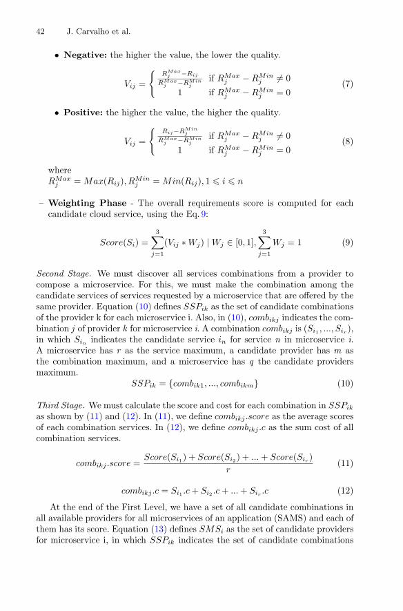
42 J. Carvalho et al.
• Negative: the higher the value, the lower the quality.
Vij =
{RMax
j −Rij
RMaxj −RMin
jif RMax
j − RMinj �= 0
1 if RMaxj − RMin
j = 0(7)
• Positive: the higher the value, the higher the quality.
Vij =
{Rij−RMin
j
RMaxj −RMin
jif RMax
j − RMinj �= 0
1 if RMaxj − RMin
j = 0(8)
whereRMax
j = Max(Rij), RMinj = Min(Rij), 1 � i � n
– Weighting Phase - The overall requirements score is computed for eachcandidate cloud service, using the Eq. 9:
Score(Si) =3∑
j=1
(Vij ∗ Wj) | Wj ∈ [0, 1],3∑
j=1
Wj = 1 (9)
Second Stage. We must discover all services combinations from a provider tocompose a microservice. For this, we must make the combination among thecandidate services of services requested by a microservice that are offered by thesame provider. Equation (10) defines SSPik as the set of candidate combinationsof the provider k for each microservice i. Also, in (10), combikj indicates the com-bination j of provider k for microservice i. A combination combikj is (Si1 , ..., Sir ),in which Sin indicates the candidate service in for service n in microservice i.A microservice has r as the service maximum, a candidate provider has m asthe combination maximum, and a microservice has q the candidate providersmaximum.
SSPik = {combik1, ..., combikm} (10)
Third Stage. We must calculate the score and cost for each combination in SSPik
as shown by (11) and (12). In (11), we define combikj .score as the average scoresof each combination services. In (12), we define combikj .c as the sum cost of allcombination services.
combikj .score =Score(Si1) + Score(Si2) + ... + Score(Sir )
r(11)
combikj .c = Si1 .c + Si2 .c + ... + Sir .c (12)
At the end of the First Level, we have a set of all candidate combinations inall available providers for all microservices of an application (SAMS) and each ofthem has its score. Equation (13) defines SMSi as the set of candidate providersfor microservice i, in which SSPik indicates the set of candidate combinations

Dynamic Selecting Approach for Multi-cloud Providers 43
of provider k for microservice i. In (14), we define SAMS as the set of candidateproviders for each microservice of an application, and an application has t asthe microservices maximum.
SMSi = {SSPik | k ∈ [1, q]} (13)
SAMS = {SMS1, ..., SMSt} (14)
Second Level - Cloud Providers Selection to Deploy Microservices. Wemust select the cloud providers from SAMS (First Level) to host each microser-vice of an application. For this, we must make the combination among the candi-date combinations SAMS, in which each combination has one candidate of eachmicroservice and the set of these combinations is called SAPP (15). Also, in(15), combikijki
indicates combination j of candidate provider k for microservicei. Afterwards, (16), we define SAPPl.c as the execution cost of each combinationin SAPP and verify if it is less than or equal to the application execution cost,and exclude it otherwise. Next, we calculate the score of every item in SAPP.A candidate combination score (SAPPl.score) is a value among ]0, 1], and it isthe score sum of each item combination, which is shown in (17).
SAPP = {(comb1k1jk1, ..., combtktjkt
) | combikijki∈ SSPik, SSPik ∈ SMSi,
SMSi ∈ SAMS, 1 � i � t, 1 � ki � qi, 1 � jki� wki
}(15)
SAPPl.c =t∑
i=1
combikijki.c (16)
SAPPl.score =t∑
i=1
combikijki.score (17)
The selection process described above is a combinatorial optimization prob-lem and one of the most studied problems in combinatorial optimization is theknapsack problem. Hence, we map the selection process up to multi-choice knap-sack problem. The application budget represents the maximum knapsack weightand each item in SAPP has its cost, i.e., its weight. Each SAPP item representsthe set of services that are necessary for each application microservice. Thus, themicroservices represent the classes, because each item of SAPP must contain setof services for each microservice. Our selection problem must maximize the userrequirements through the score of each item in SAPP. The item score representsthe profit, (18) illustrates the objective function to maximize the score, whichis subject to (19), (20) and (21) for obeying total combination cost. In theseequations, combikj is candidate combination j of provider k for microservice i,

44 J. Carvalho et al.
SMSi is a set of candidate providers for microservice i, as defined in formula13, and SSPik is a set of combinations of provider k for each microservice i, asdefined in formula 10.
max(t∑
i=1
∑
k∈SMSi
∑
j∈SSPik
combikj .score ∗ Combikj) (18)
t∑
i=1
∑
k∈SMSi
∑
j∈SSPik
combikj .c ∗ combikj � AP.c (19)
∑
k∈SMSi
SSPik = 1,∀1 � i � t (20)
∑
j∈SSPik
combikj = 1,∀1 � i � t, k ∈ [1, q] (21)
2.3 Algorithm for Cloud Providers Selection
Next, we present Algorithm 1 for the selection process of our approach. Wherebyis possible to observe all selection process level described in this section. Algo-rithm1 has as input the set of application requirements and the set of the capa-bilities of the providers and as output set of the providers to host each applicationmicroservice. We describe an overall Algorithm 1, as follow.
1. First, we discover the provider services that meet all the requirements of amicroservice (line 4). Then, we rank them by calculating SAW Scaling Phase(line 6) and SAW Score Phase for each service (line 7). Next, we combine theservices (line 8) so that each combination has all the services required by themicroservice. The process is repeated on all available providers;
2. Next, we calculate the score (line 13) and the cost (line 14) of each com-bination. The entire process between lines 2 and 13 is repeated for all theapplication microservices, resulting in a set of candidate combinations foreach microservice (SAMS), each of them has its score and cost;
3. Finally, from line 21 to 29, we selected a combination to host a microserviceamong the candidate combinations of the microservice in SAMS. For this,we create a matrix (Sol) using lines for every possible combination cost value(from 1 to AP.c) and columns for the cost of each existing combinations.Matrix Sol is filled with the score values according to the microservice towhich the combination belongs, in order to obtain the combinations withthe highest score that, when combined, do not exceed the budget value ofthe application (AP.c), according to the mapping made for the multi-choicebackpack problem as described in (15), (16), (17), (18), (19), (20), and (21).

Dynamic Selecting Approach for Multi-cloud Providers 45
Algorithm 1. The Proposed Approachinput : Set of the application requirements ap
Set of the capabilities of the providers cpoutput : Set of Providers prvdsMs to host each microservices of an
application
1 foreach ms of the ap do2 ssp ← initialize with empty set ;3 foreach sp of the cp do4 candServ ← discoveryCandServ (ms,sp);5 if (notempty(candServ)) then6 matReq ← sawScalingPh (candServ) ; // formulas 7 and 8
7 candServSC ← sawScorePh (candServ,matReq,ap.weight) ; // formula 9
8 ssp ← ssp + (sp.number,combMsSp (candServSC)) ; // formula 10
9 end
10 end11 sms ← initialize with empty set ;12 foreach comb of the ssp do13 combSC ← calculateCombSC (comb) ; // formula 11
14 combCost ← calculateCombCost (comb) ; // formula 12
15 sms ← sms + (comb,combSC,combCost);
16 end17 sams ← sams + (ms.number,sms);
18 end// The algorithm between lines 19 and 29 indicates the cloud providers selection using dynamic
programming for mapping of the multi-choice knapsack problem.;19 sol ← initialize the matrix with values 0 ;20 last ← 1;21 foreach sms of the sams do22 for j ← last to sizeof(sms) − 1 do23 for cost ← 1 to ap.c do24 if (combCost[j] > cost) then sol(cost, j) ← sol(cost, j − 1);25 else if (ms[j].number == 1) then sol(cost, j) ← combSC[j];26 else if (ms[j].number �= ms[j − 1].number) then
sol(cost, j) ← max(maxLine(sol(cost − combCost[j]),ms[j −1].number) + combSC[j], maxLine(sol(cost),ms[j − 1].number));
27 else sol(cost, j,ms[j].number) ←max(maxLine(sol(cost − combCost[j]),ms[j].number − 1) +combSC[j], maxLine(sol(cost),ms[j].number − 1));
28 end29 last ← sizeof(sms);
30 end
31 end

46 J. Carvalho et al.
3 Evaluation
We have developed a tool and set up scenarios to evaluate our approach. In thissection, we describe how the tool was implemented, the scenarios configuration,the experiments, and the outcomes.
3.1 Tool Description
The tool was implemented using python 3.7 and we used the JSON formatas input and output. The tool has two JSON files as input: one contains theservice providers capabilities and the other has the application requirements.Each provider capabilities are organized by service classes, in which each class hasits services. We consider three classes of services: compute, storage and database.Each service must contain its functional and non-functional capabilities. Thenonfunctional capabilities we consider in our approach are availability, executiontime, delay and cost, as described in Sect. 2.
Application information involves name, minimum availability, maximumresponse time, maximum budget, weight and priority of each user requirementand the microservices information.
The tool returns a JSON file, which contains the providers that will deploythe microservices, as well as the services that will be used and the providers cost.
As previously mentioned, we map our multi-cloud selection process to themulti-choice knapsack problem, which is a highly researched combinatorial opti-mization problem. The multi-choice knapsack problem can be developed throughsome techniques, such as dynamic programming and greedy. We use dynamicprogramming in our tool.
3.2 Setting Scenarios
For tool evaluation purposes, we randomly configure six sets of providers as in [5,6,11], which differ from one another by the number of providers and each servicecapabilities. For this, we first randomly configured the set with 5 providers. Next,we configure the other set of providers from (22). In (22), SPrvdsx is a set ofproviders, in which x is the number of providers in SPrvds, and SPrvdsx−5
is the set of providers configured with the highest number of providers up tothat moment according to the proposed scenario, and x must be higher than orequal to 5. If x is equal 5 indicates that is the first set of the scenario then x== 0 is the empty set. For example, if x == 15 then the set of 15 providers isbased on the set of 10 providers previously configured. Each provider has threeservices classes: compute, storage and database, and each class has six services.The amount of providers in each set is a multiple value of 5, in which the firstset has 5 providers and the last 30.
SPrvdsx = SPrvds(x−5) + SPrvds5 (22)
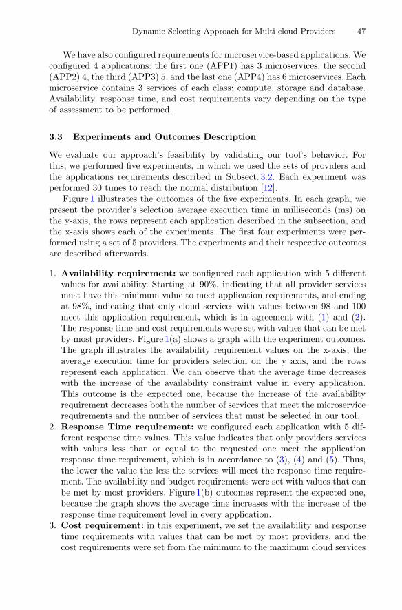
Dynamic Selecting Approach for Multi-cloud Providers 47
We have also configured requirements for microservice-based applications. Weconfigured 4 applications: the first one (APP1) has 3 microservices, the second(APP2) 4, the third (APP3) 5, and the last one (APP4) has 6 microservices. Eachmicroservice contains 3 services of each class: compute, storage and database.Availability, response time, and cost requirements vary depending on the typeof assessment to be performed.
3.3 Experiments and Outcomes Description
We evaluate our approach’s feasibility by validating our tool’s behavior. Forthis, we performed five experiments, in which we used the sets of providers andthe applications requirements described in Subsect. 3.2. Each experiment wasperformed 30 times to reach the normal distribution [12].
Figure 1 illustrates the outcomes of the five experiments. In each graph, wepresent the provider’s selection average execution time in milliseconds (ms) onthe y-axis, the rows represent each application described in the subsection, andthe x-axis shows each of the experiments. The first four experiments were per-formed using a set of 5 providers. The experiments and their respective outcomesare described afterwards.
1. Availability requirement: we configured each application with 5 differentvalues for availability. Starting at 90%, indicating that all provider servicesmust have this minimum value to meet application requirements, and endingat 98%, indicating that only cloud services with values between 98 and 100meet this application requirement, which is in agreement with (1) and (2).The response time and cost requirements were set with values that can be metby most providers. Figure 1(a) shows a graph with the experiment outcomes.The graph illustrates the availability requirement values on the x-axis, theaverage execution time for providers selection on the y axis, and the rowsrepresent each application. We can observe that the average time decreaseswith the increase of the availability constraint value in every application.This outcome is the expected one, because the increase of the availabilityrequirement decreases both the number of services that meet the microservicerequirements and the number of services that must be selected in our tool.
2. Response Time requirement: we configured each application with 5 dif-ferent response time values. This value indicates that only providers serviceswith values less than or equal to the requested one meet the applicationresponse time requirement, which is in accordance to (3), (4) and (5). Thus,the lower the value the less the services will meet the response time require-ment. The availability and budget requirements were set with values that canbe met by most providers. Figure 1(b) outcomes represent the expected one,because the graph shows the average time increases with the increase of theresponse time requirement level in every application.
3. Cost requirement: in this experiment, we set the availability and responsetime requirements with values that can be met by most providers, and thecost requirements were set from the minimum to the maximum cloud services

48 J. Carvalho et al.
Fig. 1. Cloud providers selection execution time (a) application availability; (b) appli-cation response time; (c) application budget; (d) application user requirement class;and (e) set of providers.
values. Thus, the values in the x-axis represent budget classes, and each classhas different budget values for each application, but all applications have thesame value per service in each class. The budget value per class is different ineach application, but the applications have the same value per service in each

Dynamic Selecting Approach for Multi-cloud Providers 49
class. Also, class 1 has the lowest value per service, class 2 has a value higherthan class 1 but lower than the class 3, and last class has the highest valueper service. The lowest and highest values per service are based on the lowestand highest value of the set of providers described in this scenario. Class 1 hasthe minimum value and a class 7 has the maximum value. Therefore, no set ofproviders meet the budget with a value lower than class 1, and all providersmet budget with values higher than class 7. The budget values indicate thatonly cloud services with values less than or equal to the attributed ones meetthe cost requirement as described in (6). Figure 1(c) outcomes show thatthe average execution time increases alongside with the cost level, but after acertain amount the average execution time is stabilized. This happens becausethe higher the budget, the greater the search for a better solution.
4. User requirements: in these experiments we vary all three constraints:availability, response time and cost, in a manner that when the availabil-ity requirement increases, the cost and response time requirements decrease.Therefore, when the requirements class is increased on the x-axis of Fig. 1(d),we say that the constraints increases. Thus, we can observe that the averageexecution time in the graph decreases with the increase of the requirements.This outcome shows that the increase of the requirements reduces the numberof providers that meet all requirements and that the average execution timeconverges to the same value.
5. Set of Providers: for this experiment we set up 5 set of providers, each witha multiple of 5 as the number of providers, in such manner that the first set has10 providers and the last one has 30 providers, which have been configuredaccording to (22). The requirements of availability, response time and costwere not modified during the experiment, maintaining the same value in allsets. Those requirements were configured using the intermediate values, i.e.,they have neither the lowest nor the highest constraint. We can see in Fig. 1(e)that the increase in the number of providers influences the average selectiontime, since it increases the number of services that meet the applicationsrequirements. Also, we can observe that the amount of microservices alsoinfluences the cloud providers selection average time.
As mentioned in Sect. 1, in the literature there are dealing with the cloudprovider selection, but the focus of these works is different from ours. Some ofthem select one provider per application or service flow, and others are basedon the cloud federation environment, which there is a collaboration agreementbetween providers. Besides, there is still one that deals with cloud selection tohost microservice, but each service to microservice is hosted on a different cloudprovider. The comparison of our proposal with these works is complex becauseeach proposal has different purposes.
4 Related Work
Despite the growth of cloud computing, multiple clouds are still at their begin-ning [13], and very few research works related to cloud providers selections exist.In this Section, we compare our work with some of these previous works.
50 J. Carvalho et al.
Wang et al. [5] proposed a service selection based on correlated QoS require-ments, in which each service belongs to the same provider. Similarly to our work,[5] organizes the services within the provider by classes and considers that eachrequired service belongs to a class and that several services candidates exist andeach of them possesses the same functionality but different capabilities. Liu et al.[6] organizes services within the providers as our work does, but it proposed aservice flow scheduling model with multiple service requirements in a cloud.
Zeng et al. [7] proposed a middleware which addresses the issue of selectingweb services for their composition in a manner that maximizes user requirements.[7] leads the problems related to service selection the same way our work does.
Pietrabissa et al. [8] proposed a cloud resource allocation algorithm thatmanages the resource requests with the aim of maximizing the Cloud Man-ager Broker (CMB) revenue over time, focusing on the provider perspective andresource allocation in cloud federation, while our work focus on user perspectiveand multi-cloud environment.
Garg et al. [11] proposed a framework and mechanism that allow the evalu-ation of cloud offerings and rank them based on their ability to meet the user’srequirements. Hence, the framework may permit a competition among cloudproviders to satisfy their SLA and improve their QoS. This work differs fromours because we select the providers that best meet the user’s requirements foreach microservice of an application.
Sousa et al. [9] proposed an automated approach for the selection and con-figuration of cloud providers in multi-cloud microservices-based applications. [9]is similar to our work, but while [9] selects the services of a microservice inseveral providers, our work selects a provider to a microservice. Our work isbased on Multi-Criteria Decision Making Methods (MCDM), while [9] is basedon ontology reasoning and software product line techniques.
5 Conclusion
In this paper, we propose and formally describe a multiple cloud provider selec-tion approach for PacificClouds, which must select the providers that best meetuser requirements for each microservice of an application. We also use SAWto rank the candidate services for each microservice in each of the availableproviders according to its requirements. In addition, we mapped the providerselection process to the multi-choice knapsack problem. As a result, we havedeveloped a tool that represents the proposed approach and we use dynamicprogramming to implement the multi-choice knapsack problem, then we evalu-ate the proposed approach using the developed tool. The outcomes show that theapproach finds the best solution and that the approach proved to be viable evenin the face of extreme restrictions. For future works, we intend to develop theprovider selection process by using the knapsack problem via greedy algorithm,then we intend to compare it with this approach.

Dynamic Selecting Approach for Multi-cloud Providers 51
References
1. Mezgar, I., Rauschecker, U.: The challenge of networked enterprises for cloud com-puting interoperability. Comput. Ind. 65(4), 657–674 (2014)
2. Silva, G.C., Rose, L.M., Calinescu, R.: A systematic review of cloud lock-in solu-tions. In: 2013 IEEE 5th International Conference on Cloud Computing Technologyand Science, pp. 363–368 (2013)
3. Petcu, D.: Multi-cloud: expectations and current approaches. In: Proceedings of the2013 International Workshop on Multi-cloud Applications and Federated Clouds,MultiCloud 2013, pp. 1–6 (2013)
4. Carvalho, J.O.D., Trinta, F., Vieira, D.: PacificClouds : a flexible MicroServicesbased architecture for interoperability in multi-cloud environments. In: CLOSER2018, pp. 448–455 (2018)
5. Wang, Y., He, Q., Ye, D., Yang, Y.: Service selection based on correlated QoSrequirements. In: 2017 IEEE International Conference on Services Computing(SCC), pp. 241–248 (2017)
6. Liu, H., Xu, D., Miao, H.K.: Ant colony optimization based service flow schedulingwith various QoS requirements in cloud computing. In: Proceedings of the 1st ACISInternational Symposium on Software and Network Engineering, SSNE 2011, pp.53–58 (2011)
7. Zeng, L., Benatallah, B., Ngu, A.H., Dumas, M., Kalagnanam, J., Chang, H.: QoS-aware middleware for web services composition. IEEE Trans. Softw. Eng. 30(5),311–327 (2004)
8. Pietrabissa, A., Priscoli, F.D., Di Giorgio, A., Giuseppi, A., Panfili, M., Suraci,V.: An approximate dynamic programming approach to resource management inmulti-cloud scenarios. Int. J. Control 90(3), 508–519 (2017)
9. Sousa, G., Rudametkin, W., Duchien, L.: Automated setup of multi-cloud environ-ments for microservices-based applications. In: 9th IEEE International Conferenceon Cloud Computing (2016)
10. Al-Faifi, A.M., Song, B., Alamri, A., Alelaiwi, A., Xiang, Y.: A survey on multi-criteria decision making methods for evaluating cloud computing services. J. Inter-net Technol. 18(3), 473–494 (2017)
11. Garg, S.K., Versteeg, S., Buyya, R.: A framework for ranking of cloud computingservices. Future Gen. Comput. Syst. 29(4), 1012–1023 (2013)
12. Hogendijk, J., Whiteside, A.E.S.D.: Sources and Studies in the History of Mathe-matics and Physical Sciences. Springer US (2011)
13. Petcu, D.: Consuming resources and services from multiple clouds. J. Grid Comput.12(2), 321–345 (2014)

Research Track: Cloud Data Storage
Teleporting Failed Writes with CacheAugmented Data Stores
Shahram Ghandeharizadeh(B), Haoyu Huang, and Hieu Nguyen
USC Database Laboratory, Los Angeles, USA{shahram,haoyuhua,hieun}@usc.edu
Abstract. Cache Augmented Data Stores enhance the performance ofworkloads that exhibit a high read to write ratio by extending a persistentdata store (PStore) with a cache. When the PStore is unavailable, today’ssystems result in failed writes. With the cache available, we proposeTARDIS, a family of techniques that teleport failed writes by bufferingthem in the cache and persisting them once the PStore becomes available.TARDIS preserves consistency of the application reads and writes byprocessing them in the context of buffered writes. TARDIS family oftechniques is differentiated in how they apply buffered writes to PStoreonce it recovers. Each technique requires a different amount of mappinginformation for the writes performed while PStore was unavailable. Theprimary contribution of this study is an overview of TARDIS and itsfamily of techniques.
1 Introduction
Person-to-person cloud service providers such as Facebook challenge today’s soft-ware and hardware infrastructure [9,24]. Traditional web architectures struggleto process their large volume of requests issued by hundreds of millions of users.In addition to facilitating a near real-time communication, a social networkinfrastructure must provide an always-on experience in the presence of differ-ent forms of failure [9]. These requirements have motivated an architecture thataugments a data store with a distributed in-memory cache manager such asmemcached and Redis. We term this class of systems Cache Augmented DataStores, CADSs.
Figure 1 shows a CADS consisting of Application Node (AppNode) serversthat store and retrieve data from a persistent store (PStore) and use a cache fortemporary staging of data [18,24,25]. The cache expedites processing of requestsby either using faster storage medium, bringing data closer to the AppNode, or acombination of the two. An example PStore is a document store [10] that is eithera solution such as MongoDB or a service such as Amazon DynamoDB [5,11] orMongoDB’s Atlas [22]. An example cache is an in-memory key-value store suchas memcached or Redis with Amazon ElastiCache [6] as an example service.Both the caching layer and PStore may employ data redundancy techniques totolerate node failures.c© Springer International Publishing AG, part of Springer Nature 2018M. Luo and L.-J. Zhang (Eds.): CLOUD 2018, LNCS 10967, pp. 55–68, 2018.https://doi.org/10.1007/978-3-319-94295-7_4
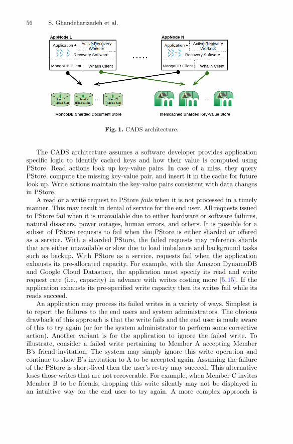
56 S. Ghandeharizadeh et al.
Fig. 1. CADS architecture.
The CADS architecture assumes a software developer provides applicationspecific logic to identify cached keys and how their value is computed usingPStore. Read actions look up key-value pairs. In case of a miss, they queryPStore, compute the missing key-value pair, and insert it in the cache for futurelook up. Write actions maintain the key-value pairs consistent with data changesin PStore.
A read or a write request to PStore fails when it is not processed in a timelymanner. This may result in denial of service for the end user. All requests issuedto PStore fail when it is unavailable due to either hardware or software failures,natural disasters, power outages, human errors, and others. It is possible for asubset of PStore requests to fail when the PStore is either sharded or offeredas a service. With a sharded PStore, the failed requests may reference shardsthat are either unavailable or slow due to load imbalance and background taskssuch as backup. With PStore as a service, requests fail when the applicationexhausts its pre-allocated capacity. For example, with the Amazon DynamoDBand Google Cloud Datastore, the application must specify its read and writerequest rate (i.e., capacity) in advance with writes costing more [5,15]. If theapplication exhausts its pre-specified write capacity then its writes fail while itsreads succeed.
An application may process its failed writes in a variety of ways. Simplest isto report the failures to the end users and system administrators. The obviousdrawback of this approach is that the write fails and the end user is made awareof this to try again (or for the system administrator to perform some correctiveaction). Another variant is for the application to ignore the failed write. Toillustrate, consider a failed write pertaining to Member A accepting MemberB’s friend invitation. The system may simply ignore this write operation andcontinue to show B’s invitation to A to be accepted again. Assuming the failureof the PStore is short-lived then the user’s re-try may succeed. This alternativeloses those writes that are not recoverable. For example, when Member C invitesMember B to be friends, dropping this write silently may not be displayed inan intuitive way for the end user to try again. A more complex approach is

Teleporting Failed Writes with Cache Augmented Data Stores 57
for the application to buffer the failed writes. A system administrator wouldsubsequently process and recover these writes.
This paper describes an automated solution that replaces the administratorwith a smart algorithm that buffers failed writes and applies them to PStore at alater time once it is available. This approach constitutes the focus of TARDIS1,a family of techniques for processing failed writes that are transparent to theuser issuing actions.
Table 1. Number of failed writes with different BG workloads and PStore failuredurations.
Failure duration Read to write ratio
100:1 1000:1
1min 5,957 561
5min 34,019 3,070
10min 71,359 6,383
TARDIS teleports failed writes by buffering them in the cache and performingthem once the PStore is available. Buffered writes stored as key-value pairs inthe cache are pinned to prevent the cache from evicting them. To tolerate cacheserver failures, TARDIS replicates buffered writes across multiple cache servers.
Table 1 shows the number of failed writes with different failure durationsusing a benchmark for interactive social networking actions named BG [8]. Weconsider two workloads with different read to write ratios. TARDIS teleports allfailed writes and persists them once PStore becomes available.
TARDIS addresses the following challenges:
1. How to process PStore reads with pending buffered writes in the cache?2. How to apply buffered writes to PStore while servicing end user requests in
a timely manner?3. How to process non-idempotent buffered writes with repeated failures during
recovery phase?4. What techniques to employ to enable TARDIS to scale? TARDIS must dis-
tribute load of failed writes evenly across the cache instances. Moreover, itsimposed overhead must be minimal and independent of the number of cacheservers.
TARDIS preserves consistency guarantees of its target application while tele-porting failed writes. This is a significant improvement when compared withtoday’s state of the art that loses failed writes always.
Advantages of TARDIS are two folds. First, it buffers failed writes in thecache when PStore is unavailable and applies them to PStore once it becomes1 Time and Relative Dimension in Space, TARDIS, is a fictional time machine and
spacecraft that appears in the British science fiction television show Doctor Who.

58 S. Ghandeharizadeh et al.
available. Second, it enhances productivity of application developers and systemadministrators by providing a universal framework to process failed writes. Thissaves both time and money by minimizing complexity of the application software.
Assumptions of TARDIS include:
– AppNodes and the cache servers are in the same data center, communicatingusing a low latency network. This is a reasonable assumption because cachesare deployed to enhance AppNode performance.
– The cache is available to an AppNode when PStore writes fail.– A developer authors software to reconstruct a PStore document using one or
more cached key-value pairs. This is the recovery software shown in Fig. 1used by both the application software and Active Recovery (AR) workers.
– The PStore write operations are at the granularity of a single document andtransition its state from one consistent state to another. In essence, the cor-rectness of PStore writes are the responsibility of the application developer.
– There is no dependence between two or more buffered writes applied to differ-ent2 documents. This is consistent with the design of a document store suchas MongoDB to scale horizontally. Extensions to a relational data model thatconsiders foreign key constraints is a future research direction.
Fig. 2. AppNode state transition diagram.
The rest of this paper is organized as follows. Section 2 presents the design ofTARDIS. Section 3 describes how undesirable race conditions may happen andour solution using contextual leases. We survey related work in Sect. 4. Brieffuture research directions are presented in Sect. 5.
2 TARDIS preserves the order of two or more writes for the same document.

Teleporting Failed Writes with Cache Augmented Data Stores 59
2 Overview
Each AppNode in TARDIS operates in 3 distinct modes: normal, failed, andrecovery. Figure 2 shows the state transition diagram for these three modes.TARDIS operates in normal mode as long as PStore processes writes in a timelymanner. A failed PStore write transitions AppNode to failed mode. In this mode,AppNode threads buffer their PStore writes in the cache. They maintain cachedkey-value pair impacted by the write as in normal mode of operation. Moreover,the AppNode starts one or more Active Recovery (AR) workers to detect whenthe PStore is available to process writes again. Once PStore processes a writeby an AR worker, the AR worker transitions AppNode state to recovery mode.
In recovery mode, TARDIS applies buffered writes to PStore. TARDIS familyof techniques is differentiated in how they perform this task. In its simplest form,termed TAR, only AR workers apply buffered writes. The next variant, termedDIS, extends TAR by requiring the write actions of the application to identifypending writes in the cache and apply them to PStore prior to performing theirwrite. With DIS, a write action may merge the pending writes with its own intoone PStore operation. With TARD, the developer provides a mapping betweenthe read and buffered writes produced by write actions. This mapping enablesthe application to process reads that observe a cache miss by first applying thepending buffered writes to the PStore. Finally, TARDIS is a hybrid that includesfeatures of both TARD and DIS.
The trade-off with the alternative techniques is as follows. With TAR, theapplication continues to produce buffered writes even though PStore is available.With both TAR and DIS, a cache miss continues to report a failure (even thoughPStore is available) until all pending writes are applied to PStore. DIS is differ-ent because it stops the application from producing buffered writes, enabling therecovery mode to end sooner. With TARD, a cache miss applies buffered writesto PStore while writes continue to be buffered. TARDIS is most efficient in pro-cessing application requests, ending the recovery process fastest. Due to noveltyof TARDIS, applicability of TAR, TARD, DIS, and TARDIS in the context ofdifferent applications is a future research direction. It may be the case that DISis applicable to most if not all applications.
When either AppNode or an AR worker incurs a failed write, it switchesAppNode mode from recovery to failed. A PStore that processes writes inter-mittently may cause AppNode to toggle between failed and recovery modesrepeatedly, see Fig. 2.
2.1 Failed Mode
In failed mode, a write for Di generates a change δi for this PStore document andappends δi to the buffered write Δi of the document in the cache. In addition,this write appends Pi to the value of a key named Teleported Writes, TeleW.This key-value pair is also stored in the cache. It is used by AR workers todiscover documents with pending buffered writes (Table 2).
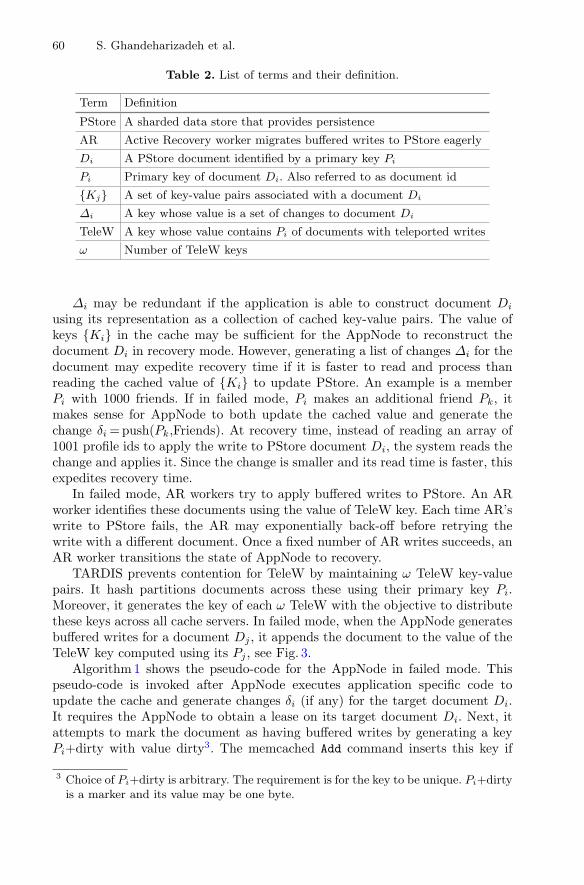
60 S. Ghandeharizadeh et al.
Table 2. List of terms and their definition.
Term Definition
PStore A sharded data store that provides persistence
AR Active Recovery worker migrates buffered writes to PStore eagerly
Di A PStore document identified by a primary key Pi
Pi Primary key of document Di. Also referred to as document id
{Kj} A set of key-value pairs associated with a document Di
Δi A key whose value is a set of changes to document Di
TeleW A key whose value contains Pi of documents with teleported writes
ω Number of TeleW keys
Δi may be redundant if the application is able to construct document Di
using its representation as a collection of cached key-value pairs. The value ofkeys {Ki} in the cache may be sufficient for the AppNode to reconstruct thedocument Di in recovery mode. However, generating a list of changes Δi for thedocument may expedite recovery time if it is faster to read and process thanreading the cached value of {Ki} to update PStore. An example is a memberPi with 1000 friends. If in failed mode, Pi makes an additional friend Pk, itmakes sense for AppNode to both update the cached value and generate thechange δi = push(Pk,Friends). At recovery time, instead of reading an array of1001 profile ids to apply the write to PStore document Di, the system reads thechange and applies it. Since the change is smaller and its read time is faster, thisexpedites recovery time.
In failed mode, AR workers try to apply buffered writes to PStore. An ARworker identifies these documents using the value of TeleW key. Each time AR’swrite to PStore fails, the AR may exponentially back-off before retrying thewrite with a different document. Once a fixed number of AR writes succeeds, anAR worker transitions the state of AppNode to recovery.
TARDIS prevents contention for TeleW by maintaining ω TeleW key-valuepairs. It hash partitions documents across these using their primary key Pi.Moreover, it generates the key of each ω TeleW with the objective to distributethese keys across all cache servers. In failed mode, when the AppNode generatesbuffered writes for a document Dj , it appends the document to the value of theTeleW key computed using its Pj , see Fig. 3.
Algorithm 1 shows the pseudo-code for the AppNode in failed mode. Thispseudo-code is invoked after AppNode executes application specific code toupdate the cache and generate changes δi (if any) for the target document Di.It requires the AppNode to obtain a lease on its target document Di. Next, itattempts to mark the document as having buffered writes by generating a keyPi+dirty with value dirty3. The memcached Add command inserts this key if
3 Choice of Pi+dirty is arbitrary. The requirement is for the key to be unique. Pi+dirtyis a marker and its value may be one byte.

Teleporting Failed Writes with Cache Augmented Data Stores 61
Fig. 3. Documents are partitioned across ω TeleW keys. TeleW keys are sharded acrossq memcached servers.
it does not exist. Otherwise, it returns NOT STORED. Hence, the first timea document is inserted, it is appended to one of the ω TeleW keys. Repeatedwrites of Di in failed mode do not insert a document Di in TeleW again.
Algorithm 1. AppNode in Failed Mode (Pi)1. acquire lease Pi
2. InsertAttempt = Add(Pi+dirty)3. release lease Pi
4. if InsertAttempt is successful {TeleWi = hash(Pi, ω)acquire lease TeleWi
append(Pi, TeleWi)release lease TeleWi
}
2.2 Recovery Mode
To perform an action that references a document Di, AppNode checks to see ifthis document has buffered writes. It does so by obtaining a lease on Pi. Oncethe lease is granted, it looks up Δi. If it does not exist then it means an ARworker (or another AppNode thread) competed with it and propagated Di’schanges to PStore. In this case, it releases its lease and proceeds to service user’saction. Otherwise, it applies the buffered writes to update Di in PStore. If this issuccessful, AppNode deletes Δi to prevent an AR worker from applying bufferedwrites to Di a second time.
TARDIS employs AR workers to eagerly apply buffered writes to PStore doc-uments identified by TeleW. We minimize the recovery duration by maximizing
62 S. Ghandeharizadeh et al.
the probability of each AR worker to work on a disjoint set of documents. Toachieve this, each AR worker randomly pick TeleW key as the starting pointand visit other TeleW keys in a round-robin fashion. Also, it only recover α ran-domly selected documents in a TeleW. With AppNode, each time a user actionreferences a document Di with buffered writes, the AppNode applies its writesto the PStore prior to servicing the user action. In essence, during recovery,the AppNode stops producing buffered writes and propagates buffered writes toPStore.
Challenges of implementing TARDIS’s recovery mode is two folds: (a) cor-rectness: TARDIS must propagate buffered writes to PStore documents in aconsistent manner, and (b) performance: TARDIS must process user’s actionsas fast as normal mode while completing recovery quickly.
We categorize buffered writes into idempotent and non-idempotent. Idempo-tent writes can be repeated multiple times and produce the same value. Non-idempotent writes lack this behavior. During recovery, multiple AR workers mayperform idempotent writes multiple times without compromising correctness.However, this redundant work slows down the PStore for processing regularrequests and makes the duration of recovery longer than necessary. Our imple-mentation of recovery uses leases to apply buffered writes of a document toPStore exactly once even in the presence of AR worker or AppNode failures.The details are provided in the full technical report [26].
Algorithm 2 shows each iteration of AR worker in recovery mode. An ARworker picks a TeleW key randomly and looks up its value. This value is a list ofdocuments written in failed mode. From this list, it selects α random documents{D}. For each document Di, it looks up Pi+dirty to determine if its bufferedwrites still exist in the cache. If this key exists then it acquires a lease on Di,and looks up Pi+dirty a second time. If this key still exists then it proceeds toapply the buffered writes to Di in PStore. Should this PStore write succeed, theAR worker deletes Pi+dirty and buffered writes from the cache.
The AR worker maintains the primary key of those documents it successfullywrites to PStore in the set R. It is possible for the AR worker’s PStore write toDi to fail. In this case, the document is not added R, leaving its changes in thecache to be applied once PStore is able to do so.
An iteration of the AR worker ends by removing the documents in R (if any)from its target TeleW key, Step 6 of Algorithm 2. Duplicate Pis may exist inTeleWT . A race condition involving AppNode and AR worker generates theseduplicates: A buffered write is generated between Steps 5 and 6 of Algorithm2.Step 6 does a multi-get for TeleWT and the processed Pi+dirty values. For thosePis with a buffered write, it does not remove them from TeleWT value becausethey were inserted due to the race condition.
2.3 Cache Server Failures
A cache server failure makes buffered writes unavailable, potentially losing con-tent of volatile memory all together. To maintain availability of buffered writes,

Teleporting Failed Writes with Cache Augmented Data Stores 63
Algorithm 2. Each Iteration of AR Worker in Recovery Mode1. Initialize R = {}2. T = A random value between 0 and ω3. V = get(TeleWT )4. {D} = Select α random documents from V
5. for each Di in {D} do {V = get(Pi+dirty)if V exists {
acquire lease Pi
V = get(Pi+dirty)if V exists {
success = Update Pi in PStore with buffered writesif success {
Delete(Pi+dirty)Delete Δi (if any)R = R ∪ Pi
}} else R = R ∪ Pi
release lease Pi
} else R = R ∪ Pi
}
6. if R is not empty {acquire lease TeleWT
Do a multiget on TeleWT and all Pi+dirty in R
V = value fetched for TeleWT
For those Pi+dirty with a value, remove them from R
Remove documents in R from Vput(TeleWT ,V)release lease TeleWT
}
TARDIS replicates buffered writes across two or more cache servers. BothRedis [1] and memcached [2] support this feature.
A cache server such as Redis may also persist buffered writes to its localstorage, disk or flash [1]. This enables buffered writes to survive failures thatdestroy content of volatile memory. However, if a cache server fails when PStorerecovers, its contained buffered writes become unavailable and TARDIS mustsuspend all reads and writes to preserve consistency. Thus, replication is stillrequired to process reads and writes of an AppNode in recovery mode.
3 TARDIS Consistency
TARDIS consists of a large number of AppNodes. Each AppNode may operatein different modes as described in Sect. 2. While AppNode 1 operates in failed

64 S. Ghandeharizadeh et al.
or recovery mode, AppNode 2 may operate in normal mode. This may happenif AppNode 2 processes reads with 100% cache hit while AppNode 1 observes afailed write. This results in a variety of undesirable read-write and write-writerace conditions when user requests for a document are directed to AppNode 1and AppNode 2.
An example of a write-write race condition is that a user Bob who createsan Album and adds a photo to the Album. Assume Bob’s “create Album” isdirected to AppNode 1. If AppNode 1 is operating in failed mode then it buffersBob’s Album creation in the cache. Once PStore recovers and prior to propa-gating Bob’s album creation to PStore, Bob’s request to add a photo is issuedto AppNode 2. If AppNode 2 is in normal mode then it issues this write to analbum that does not exist in PStore.
An example of a read-write race condition is that Bob changes the permissionon his profile page so that his manager Alice cannot see his status. Subsequently,he updates his profile to show he is looking for a job. Assume Bob’s first actionis processed by AppNode 1 in failed mode and Bob’s profile is missing from thecache. This buffers the write as a change (Δ) in the cache. His second action,update to his profile, is directed to AppNode 2 (in normal mode) and is appliedto PStore because it just recovered and became available. Now, before AppNode1 propagates Bob’s permission change to PStore, there is a window of time forAlice to see Bob’s updated profile.
We present a solution, contextual leases, that employs stateful leases with-out requiring consensus among AppNodes. It implements the concept of ses-sions that supports atomicity across multiple keys along with commit and roll-backs. TARDIS with contextual leases maintains the three mode of operationdescribed in Sect. 2. It incorporates Inhibit (I) and Quarantine (Q) leases of [13]and extends them with a marker.
Table 3. IQ lease compatibility.
Granted
I lease Q lease
Requesting I lease Back-off and retry Back-off and retry
Q lease Grant Q and void I lease Reject and abort requester
The framework of [13] requires: (1) a cache miss to obtain an I lease on itsreferenced key prior to querying the PStore to populate the cache, and (2) acache update to obtain a Q lease on its referenced key prior to performing aRead-Modify-Write (R-M-W) or an incremental update such as append. Leasesare released once a session either commits or aborts. TARDIS uses the write-through policy of IQ-framework. I leases and Q leases are incompatible with eachother, see Table 3. A request for an I lease must back-off and retry if the key isalready associated with another I or Q lease. A request for a Q lease may voidan existing I lease or is rejected and aborted if the key is already associated with

Teleporting Failed Writes with Cache Augmented Data Stores 65
another Q lease. IQ avoids thundering herds by requiring only one out of manyrequests that observes a cache miss to query PStore and populate the cache. Italso eliminates all read-write and write-write race conditions.
In failed mode, a write action continues to obtain a Q lease on a key priorto performing its write. However, at commit time, a Q lease is converted to a Pmarker on the key. This marker identifies the key-value pair as having bufferedwrites. The P marker serves as the context for the I and Q leases granted on akey. It has no impact on their compatibility matrix. When the AppNode requestseither an I or a Q lease on a key, if there is a P marker then the AppNode isinformed of this marker should the lease be granted. In this case, the AppNodemust recover the PStore document prior to processing the action.
In our example undesirable write-write race condition, Bob’s Album creationusing AppNode 1 generates a P marker for Bob’s Album. Bob’s addition of aphoto to the album (using AppNode 2) must obtain a Q lease on the albumthat detects the marker and requires the application of buffered writes prior toprocessing this action. Similarly, with the undesirable read-write race condition,Bob’s read (performed by AppNode 2) is a cache miss that must acquire an Ilease. This lease request detects the P marker that causes the action to processthe buffered writes. In both scenarios, when the write is applied to PStore andonce the action commits, the P marker is removed as a part of releasing the Qleases.
4 Related Work
The CAP theorem states that a system designer must choose between strongconsistency and availability in the presence of network partitions [21]. TARDISimproves availability while preserving consistency.
A weak form of data consistency known as eventual has multiple meaningsin distributed systems [28]. In the context of a system with multiple replicas ofa data item, this form of consistency implies writes to one replica will eventuallyapply to other replicas, and if all replicas receive the same set of writes, theywill have the same values for all data. Historically, it renders data available forreads and writes in the presence of network partitions that separate differentcopies of a data item from one another and cause them to diverge [11]. TARDISteleports failed writes due to either network partitions, PStore failures, or bothwhile preserving consistency.
A write-back policy buffers writes in the cache and applies them to PStoreasynchronously. It may not be possible to implement a write-back policy for allwrite actions of an application. This is because a write-back policy requires amapping between reads and writes to be able to process a cache miss by applyingthe corresponding buffered writes to the PStore prior to querying PStore for themissing cache entry. In these scenarios, with TARDIS, one may use DIS (withoutTARD) that continues to report a failure for cache misses during recovery modewhile applying buffered writes to PStore. A write-back policy does not provide
66 S. Ghandeharizadeh et al.
such flexibility. It also does not consider PStore availability. It improves perfor-mance of write-heavy workloads. TARDIS objective is to improve the availabilityof writes during PStore failure.
Everest [23] is a system designed to improve the performance of overloadedvolumes during peak load. Each Everest client has a base volume and a store set.When the base volume is overloaded, the client off-loads writes to its idle stores.When the base volume load is below a threshold, the client uses backgroundthreads to reclaim writes. Everest clients do not share store set. With TARDIS,AppNodes share the cache and may have different view of PStore, requiring con-textual leases. Moreover, its AppNode may fail during PSTore recovery, requiringconversion of non-idempotent writes into idempotent ones.
The race conditions encountered (see Sect. 3) are similar to those in geo-replicated data distributed across multiple data centers. Techniques such ascausal consistency [20] and lazy replication [19] mark writes with their causaldependencies. They wait for those dependencies to be satisfied prior to applyingthem at a replica, preserving order across two causal writes. TARDIS is differ-ent because it uses Δi to maintain the order of writes for a document Di thatobserves a cache miss and is referenced by one or more failed writes. With cachehits, the latest value of the keys reflects the order in which writes were performed.In recovery mode, TARDIS requires the AppNode to perform a read or a writeaction by either using the latest value of keys (cache hit) or Δi (cache miss)to restore the document in PStore prior to processing the action. Moreover, itemploys AR workers to propagate writes to persistent store during recovery. Ituses leases to coordinate AppNode and AR workers because its assumed datacenter setting provides a low latency network.
Numerous studies perform writes with a mobile device that caches data froma database (file) server. (See [27] as two examples.) Similar to TARDIS, thesestudies enable a write while the mobile device is disconnected from its sharedpersistent store. However, their architecture is different, making their designdecisions inappropriate for our use and vice versa. These assume a mobile deviceimplements an application with a local cache, i.e., AppNode and the cache arein one mobile device. In our environment, the cache is shared among multipleAppNodes and a write performed by one AppNode is visible to a different AppN-ode - this is not true with multiple mobile devices. Hence, we must use leasesto detect and prevent undesirable race conditions between multiple AppNodethreads issuing read and write actions to the cache, providing correctness.
Host-side Caches [4,16,17] (HsC) such as Flashcache [3] are application trans-parent caches that stage the frequently referenced disk pages onto NAND flash.These caches may be configured with either write-around, write-through, orwrite-back policy. They are an intermediary between a data store issuing readand write of blocks to devices managed by the operating system (OS). Applica-tion caches such as memcached are different than HsC because they require appli-cation specific software to maintain cached key-value pairs. TARDIS is somewhatsimilar to the write-back policy of HsC because it buffers writes in cache andpropagates them to the PStore (HsC’s disk) in the background. TARDIS is

Teleporting Failed Writes with Cache Augmented Data Stores 67
different because it applies when PStore writes fail. Elements of TARDIS canbe used to implement write-back policy with caches such as memcached, Redis,Google Guava [14], Apache Ignite [7], KOSAR [12], and others.
5 Conclusions and Future Research
TARDIS is a family of techniques designed for applications that must provide analways-on experience with low latency, e.g., social networking. In the presenceof short-lived persistent store (PStore) failures, TARDIS teleports failed writesby buffering them in the cache and applying them once PStore is available.
An immediate research direction is to conduct a comprehensive evaluation ofTARDIS and its variants (TAR, DIS, TARD) to quantify their tradeoff. Thisincludes an evaluation of replication techniques that enhance availability ofbuffered writes per discussion of Sect. 2.3.
More longer term, we intend to investigate extensions of TARDIS to thoselogical data models that result in dependence between buffered writes. To elabo-rate, rows of tables of a relational data model have dependencies such as foreignkey dependency. With these SQL systems, TARDIS must manage the depen-dence between the buffered writes to ensure they are teleported in the rightorder.
References
1. Redis. https://redis.io/2. repcached: Data Replication with Memcached. http://repcached.lab.klab.org/3. McDipper (2013). https://www.facebook.com/101513470904239204. Alabdulkarim, Y., Almaymoni, M., Cao, Z., Ghandeharizadeh, S., Nguyen, H.,
Song, L.: A comparison of flashcache with IQ-Twemcached. In: ICDE Workshops(2016)
5. Amazon DynamoDB (2016). https://aws.amazon.com/dynamodb/pricing/6. Amazon ElastiCache (2016). https://aws.amazon.com/elasticache/7. Apache: Ignite - In-Memory Data Fabric (2016). https://ignite.apache.org/8. Barahmand, S., Ghandeharizadeh, S.: BG: a benchmark to evaluate interactive
social networking actions. In: CIDR, January 20139. Bronson, N., Lento, T., Wiener, J.L.: Open data challenges at Facebook. In: ICDE
(2015)10. Cattell, R.: Scalable SQL and NoSQL data stores. SIGMOD Rec. 39, 12–27 (2011)11. Decandia, G., Hastorun, D., Jampani, M., Kakulapati, G., Lakshman, A., Pilchin,
A., Sivasubramanian, S., Vosshall, P., Vogels, W.: Dynamo: Amazon’s highly avail-able key-value store. In: SOSP (2007)
12. Ghandeharizadeh, S., et al.: A Demonstration of KOSAR: an elastic, scalable,highly available SQL middleware. In: ACM Middleware (2014)
13. Ghandeharizadeh, S., Yap, J., Nguyen, H.: Strong consistency in cache augmentedSQL systems. In: Middleware, December 2014
14. Google: Guava: Core Libraries for Java (2015). https://github.com/google/guava15. Google App Engine (2016). https://cloud.google.com/appengine/quotas/

68 S. Ghandeharizadeh et al.
16. Graefe, G.: The five-minute rule twenty years later, and how flash memory changesthe rules. In: DaMoN, p. 6 (2007)
17. Holland, D.A., Angelino, E., Wald, G., Seltzer, M.I.: Flash caching on the storageclient. In: USENIXATC (2013)
18. Hu, X., Wang, X., Li, Y., Zhou, L., Luo, Y., Ding, C., Jiang, S., Wang, Z.: LAMA:optimized locality-aware memory allocation for key-value cache. In: 2015 USENIXAnnual Technical Conference (USENIX ATC 15), July 2015
19. Ladin, R., Liskov, B., Shrira, L., Ghemawat, S.: Providing high availability usinglazy replication. ACM Trans. Comput. Syst. 10(4), 360–391 (1992)
20. Lloyd, W., Freedman, M.J., Kaminsky, M., Andersen, D.G.: Don’t settle for even-tual: scalable causal consistency for wide-area storage with COPS. In: SOSP (2011)
21. Lynch, N., Gilbert, S.: Brewer’s conjecture and the feasibility of consistent, avail-able partition-tolerant web services. ACM SIGACT News 33, 51–59 (2002)
22. MongoDB Atlas (2016). https://www.mongodb.com/cloud23. Narayanan, D., Donnelly, A., Thereska, E., Elnikety, S., Rowstron, A.: Everest:
scaling down peak loads through I/O Off-loading. In: Proceedings of the 8thUSENIX Conference on Operating Systems Design and Implementation, OSDI2008, Berkeley, CA, USA, pp. 15–28. USENIX Association (2008)
24. Nishtala, R., Fugal, H., Grimm, S., Kwiatkowski, M., Lee, H., Li, H.C., McElroy,R., Paleczny, M., Peek, D., Saab, P., Stafford, D., Tung, T., Venkataramani, V.:Scaling memcache at Facebook. In: NSDI, Berkeley, CA, pp. 385–398. USENIX(2013)
25. Ports, D.R.K., Clements, A.T., Zhang, I., Madden, S., Liskov, B.: Transactionalconsistency and automatic management in an application data cache. In: OSDI.USENIX, October 2010
26. Shahram Ghandeharizadeh, H.H., Nguyen, H.: TARDIS: teleporting failed writeswith cache augmented datastores. Technical report 2017–01, USC Database Lab-oratory (2017). http://dblab.usc.edu/Users/papers/TARDIS.pdf
27. Terry, D.B., Theimer, M.M., Petersen, K., Demers, A.J., Spreitzer, M.J., Hauser,C.H.: Managing update conflicts in Bayou, a weakly connected replicated storagesystem. In: SOSP (1995)
28. Viotti, P., Vukolic, M.: Consistency in non-transactional distributed storage sys-tems. ACM Comput. Surv. 49(1) (2016)
2-Hop Eclipse: A Fast Algorithmfor Bandwidth-Efficient Data Center
Switching
Liang Liu(B), Long Gong, Sen Yang, Jun (Jim) Xu, and Lance Fortnow
Georgia Institute of Technology, Atlanta, Georgia{lliu315,gonglong,sen.yang}@gatech.edu, {jx,fortnow}@cc.gatech.edu
Abstract. A hybrid-switched data center network interconnects itsracks of servers with a combination of a fast circuit switch that a sched-ule can reconfigure at significant cost and a much slower packet switchthat a schedule can reconfigure at negligible cost. Given a traffic demandmatrix between the racks, how can we best compute a good circuit switchconfiguration schedule that meets most of the traffic demand, leaving aslittle as possible for the packet switch to handle?
In this paper we propose 2-hop Eclipse, a new hybrid switch schedulingalgorithm that strikes a much better tradeoff between the performanceof the hybrid switch and the computational complexity of the algorithm,both in theory and in simulations, than the current state of the art solu-tion Eclipse/Eclipse++.
1 Introduction
Fueled by the phenomenal growth of cloud computing services, data center net-works (DCN) continue to grow relentlessly both in size, as measured by thenumber of racks of servers it has to interconnect, and in speed, as measured bythe amount of traffic it has to transport per unit of time from/to each rack [1].A traditional data center network architecture typically consists of a three-levelmulti-rooted tree of switches that start, at the lowest level, with the Top-of-Rack(ToR) switches, that each connects a rack of servers to the network [2]. However,such an architecture has become increasingly unable to scale with the explosivegrowth in both the size and the speed of the DCN, as we can no longer increasethe transporting and switching capabilities of the underlying commodity packetswitches without increasing their costs significantly.
A cost-effective solution approach to this scalability problem, called hybridcircuit and packet switching, has received considerable research attention inrecent years [3–5]. In a hybrid-switched DCN, shown in Fig. 1, n racks of com-puters on the left hand side (LHS) are connected by both a circuit switch anda packet switch to n racks on the right hand side (RHS). Note that racks onthe LHS are an identical copy of those on the RHS; however we restrict the role
c© Springer International Publishing AG, part of Springer Nature 2018M. Luo and L.-J. Zhang (Eds.): CLOUD 2018, LNCS 10967, pp. 69–83, 2018.https://doi.org/10.1007/978-3-319-94295-7_5

70 L. Liu et al.
of the former to only transmitting data and refer to them as input ports, andrestrict the role of the latter to only receiving data and refer to them as outputports. The purpose of this duplication (of racks) and role restrictions is that theresulting hybrid data center topology can be modeled as a bipartite graph.
Fig. 1. Hybrid circuit and packetswitch
Each switch transmits data from inputports (racks on the LHS) to output ports(racks on the RHS) according to the config-uration (modeled as a bipartite matching) ofthe switch at the moment. Usually, the circuitswitch is an optical switch [3,6,7], and thepacket switch is an electronic switch. Hencethe circuit switch is typically an order of mag-nitude or more faster than the packet switch.For example, the circuit and packet switchesmight operate at the respective rates of 100Gbps and 10 Gbps per port. The flip side ofthe coin however is that the circuit switch incurs a nontrivial reconfigurationdelay δ when its configuration has to change. Depending on the underlying tech-nology of the circuit switch, δ can range from tens of microseconds to tens ofmilliseconds [3,6–9].
In this paper, we study an important optimization problem stemming fromhybrid circuit and packet switching: Given a traffic demand matrix D from inputports to output ports, how to schedule the circuit switch to best (e.g., in theshortest amount of total transmission time) meet the demand? A schedule forthe circuit switch consists of a sequence of configurations (matchings) and theirtime durations (M1, α1), (M2, α2), · · · , (MK , αK). A workable schedule shouldlet the circuit switch remove (i.e., transmit) most of the traffic demand fromD, so that every row or column sum of the remaining traffic matrix is smallenough for the packet switch to handle. Since the problem of computing theoptimal schedule for hybrid switching, in various forms, is NP-hard [10], almostall existing solutions are greedy heuristics.
1.1 State of the Art: Eclipse and Eclipse++
Since our solution builds upon the state of the art solution called Eclipse [11],we provide here a brief description of it, and its companion algorithmEclipse++ [11]. Eclipse iteratively chooses a sequence of circuit switch config-urations, one per iteration, according to the following greedy criteria: In eachiteration, Eclipse tries to extract and subtract a matching (with its duration)from the n × n traffic demand matrix D that has the largest cost-adjusted util-ity, which we will specify precisely in Sect. 3. Eclipse, like most other hybridswitching algorithms, considers and allows only direct routing in the followingsense: All circuit-switched data packets reach their respective final destinationsin one-hop (i.e., enters and exits the circuit switch only once).
However, restricting the solution strategy space to only direct routing algo-rithms may leave the circuit switch underutilized. For example, a connection
2-Hop Eclipse: A Fast Algorithm 71
(edge) from input i0 to output j0 belongs to a matching M that lasts 50µs, butat the start time of this matching, there is only 40µs worth of traffic left fortransmission from i0 to j0, leaving 10µs of “slack” (i.e., residue capacity) alongthis connection. The existence of connections (edges) with such “slacks” makesit possible to perform indirect (i.e., multi-hop) routing of remaining traffic viaone or more relay nodes through a path consisting of such edges.
Besides Albedo [12], Eclipse++ [11] is the only other work that has exploredindirect routing in hybrid switching. It was shown in [11] that optimal indirectrouting using such “slacks”, left over by a direct routing solution such as Eclipse,can be formulated as the maximum multi-commodity flow over a “slack graph”,which is NP-complete [13–16]. Eclipse++ is a greedy heuristic that converts, with“precision loss” (otherwise P = NP), this multi-commodity flow computation toa large set of shortest-path computations. Hence the computational complexityof Eclipse++ is still extremely high: Both us and the authors of [11] found thatEclipse++ is roughly three orders of magnitude more computationally expensivethan Eclipse [17] for a data center with n = 100 racks.
1.2 Our Solution
We develop a new problem formulation that allows the joint optimization of bothdirect and 2-hop indirect routing, at the same time, against the aforementionedcost-adjusted utility function. We obtain our solution, called 2-hop Eclipse, byapplying the Eclipse algorithm as basis for a greedy heuristic to this new opti-mization problem. This 2-hop Eclipse algorithm, a slight yet subtle modificationof Eclipse, has the same asymptotic computational complexity and comparableexecution time as Eclipse, but has higher performance gains over Eclipse thanEclipse++, despite the fact that Eclipse++ is three orders of magnitude morecomputationally expensive.
We emphasize that 2-hop Eclipse uses a very different strategy thanEclipse++ and in particular has no resemblance to “Eclipse++ restricted to2-hops”, which according to our simulations performs slightly worse than, andhas almost the same computational complexity as unrestricted Eclipse++.
The rest of the paper is organized as follows. In Sect. 2, we describe thesystem model and the design objective of this hybrid switch scheduling problemin details. In Sect. 3, we provides a more detailed description of Eclipse [11].In Sect. 4, we present our solution, 2-hop Eclipse. In Sect. 5, we evaluate theperformance of our solution against Eclipse and Eclipse++. Finally, we describerelated work in Sect. 6 and conclude the paper in Sect. 7.
2 System Model and Problem Statement
In this section, we formulate the problem of hybrid circuit and packet switchingprecisely. We first specify the aforementioned traffic demand traffic D precisely.Borrowing the term virtual output queue (VOQ) from the crossbar switchingliterature [18], we refer to, the set of packets that arrive at input port i and

72 L. Liu et al.
are destined for output j, as VOQ(i, j). The demand matrix entry D(i, j) isthe amount of VOQ(i, j) traffic, within a scheduling window, that needs to bescheduled for transmission by the hybrid switch. It was effectively assumed, in allprior works on hybrid switching except Albedo [12] (to be discussed in Sect. 6.1),that the demand matrix D is precisely known before the computation of thecircuit switch schedule begins (say at time t). Consequently, all prior hybridswitching algorithms except Albedo [12] perform only batch scheduling of thisD. In other words, given a demand matrix D, the schedules of the circuit andthe packet switches are computed before the transmissions of the batch (i.e.,traffic in D) actually happen. Our 2-hop Eclipse algorithm also assumes that Dis precisely known in advance and is designed for batch scheduling only. Sincebatch scheduling is offline in nature (i.e., requires no irrevocable online decision-making), 2-hop Eclipse algorithm is allowed to “travel back in time” and modifythe schedules of the packet and the circuit switches as needed.
In this work, we study this problem of hybrid switch scheduling under thefollowing standard formulation that was introduced in [19]: to minimize theamount of time for the circuit and the packet switches working together totransmit a given traffic demand matrix D. We refer to this amount of timeas transmission time throughout this paper. A schedule of the circuit switchconsists of a sequence of circuit switch configurations and their durations:(M1, α1), (M2, α2), · · · , (MK , αK). Each Mk is an n × n permutation (match-ing) matrix; Mk(i, j) = 1 if input i is connected to output j and Mk(i, j) = 0otherwise. The total transmission time of the above schedule is Kδ +
∑Kk=1 αk,
where δ is the reconfiguration delay, K is the total number of configurations inthe schedule.
Since computing the optimal circuit switch schedule alone (i.e., when thereis no packet switch), in its full generality, is NP-hard [10], almost all existingsolutions are greedy heuristics. Indeed, the typical workloads we see in datacenters exhibit two characteristics that are favorable to such greedy heuristics:sparsity (the vast majority of the demand matrix elements have value 0 or closeto 0) and skewness (few large elements in a row or column account for themajority of the row or column sum) [19].
3 Background on Eclipse
Since our 2-hop Eclipse algorithm builds upon Eclipse [11], we provide herea more detailed description of Eclipse. Eclipse iteratively chooses a sequenceof configurations, one per iteration, according to the following greedy criteria:In each iteration, Eclipse tries to extract and subtract a matching from thedemand matrix D that has the largest cost-adjusted utility, defined as follows.For a configuration (M,α) (using a permutation matrix M for a duration of α),its utility U(M,α), before adjusting for cost, is U(M,α) � ‖min(αM,Drem)‖1,where Drem denotes what remains of the traffic demand (matrix) D after wesubtract from it the amounts of traffic to be served by the circuit switch accordingto the previous matchings, i.e., those computed in the previous iterations. Note
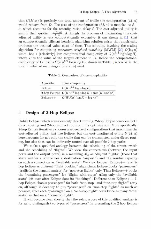
2-Hop Eclipse: A Fast Algorithm 73
that U(M,α) is precisely the total amount of traffic the configuration (M,α)would remove from D. The cost of the configuration (M,α) is modeled as δ +α, which accounts for the reconfiguration delay δ. The cost-adjusted utility issimply their quotient U(M,α)
δ+α . Although the problem of maximizing this cost-adjusted utility is very computationally expensive, it was shown in [11] thatan computationally efficient heuristic algorithm solution exists that empiricallyproduces the optimal value most of time. This solution, invoking the scalingalgorithm for computing maximum weighted matching (MWM) [20] O(log n)times, has a (relatively) low computational complexity of O(n5/2 log n log B),where B is the value of the largest element in D. Hence the computationalcomplexity of Eclipse is O(Kn5/2 log n log B), shown in Table 1, where K is thetotal number of matchings (iterations) used.
Table 1. Comparison of time complexities
Algorithm Time complexity
Eclipse O(Kn5/2 log n log B)
2-hop Eclipse O(Kn5/2 log n log B + min(K, n)Kn2)
Eclipse++ O(WKn3(log K + log n)2)
4 Design of 2-Hop Eclipse
Unlike Eclipse, which considers only direct routing, 2-hop Eclipse considers bothdirect routing and 2-hop indirect routing in its optimization. More specifically,2-hop Eclipse iteratively chooses a sequence of configurations that maximizes thecost-adjusted utility, just like Eclipse, but the cost-unadjusted utility U(M,α)here accounts for not only the traffic that can be transmitted under direct rout-ing, but also that can be indirectly routed over all possible 2-hop paths.
We make a qualified analogy between this scheduling of the circuit switchand the scheduling of “flights”. We view the connections (between the inputports and the output ports) in a matching Mk as “disjoint flights” (those thatshare neither a source nor a destination “airport”) and the residue capacityon such a connection as “available seats”. We view Eclipse, Eclipse++, and 2-hop Eclipse as different “flight booking” algorithms. Eclipse books “passengers”(traffic in the demand matrix) for “non-stop flights” only. Then Eclipse++ booksthe “remaining passengers” for “flights with stops” using only the “availableseats” left over after Eclipse does its “bookings”. Different than Eclipse++, 2-hop Eclipse “books passengers” for both “non-stop” and “one-stop flights” earlyon, although it does try to put “passengers” on “non-stop flights” as much aspossible, since each “passenger” on a “one-stop flight” costs twice as many “totalseats” as that on a “non-stop flight”.
It will become clear shortly that the sole purpose of this qualified analogy isfor us to distinguish two types of “passengers” in presenting the 2-hop Eclipse

74 L. Liu et al.
Algorithm 1: 2-hop EclipseInput: Traffic demand D;Output: Sequence of schedules (Mk, αk)k=1,...,K ;
1 sch ← {}; � schedule2 D rem ← D; � remaining demand3 R ← 0; � residue capacity4 tc ← 0; � transmission time of circuit switch5 while ∃ any row or column sum of D rem > rptc do6 Construct I rem from (D rem, R); � 2-hop demand matrix
7 (M, α) ← arg maxM∈M,α∈R+
‖ min(αM,Drem+Irem)‖1δ+α
;
8 sch ← sch ∪ {(M, α)};9 tc ← tc + δ + α;
10 Update Drem;11 Update R;
12 end
algorithm: those “looking for a non-stop flight” whose counts are encoded as theremaining demand matrix Drem, and those “looking for a connection flight” tocomplete their potential “one-stop itineraries”, whose counts are encoded as anew n × n matrix Irem that we will describe shortly. We emphasize that thisanalogy shall not be stretched any further, since it would otherwise lead toabsurd inferences, such as that such a set of disjoint “flights” must span thesame time duration and have the same number of “seats” on them.
4.1 The Pseudocode
The pseudocode of 2-hop Eclipse is shown in Algorithm1. It is almost identi-cal to that of Eclipse [11]. The only major difference is that in each iteration(of the “while” loop), 2-hop Eclipse searches for a matching (M,α) that max-imizes ‖min(αM, Drem+Irem)‖1
δ+α , whereas Eclipse searches for one that maximizes‖min(αM, Drem)‖1
δ+α . In other words, in each iteration, 2-hop Eclipse first performssome preprocessing to obtain Irem and then substitute the parameter Drem byDrem + Irem in making the “argmax” call (Line 7). The “while” loop of Algo-rithm1 terminates when every row or column sum of Drem is no more than rptc,where rp denotes the (per-port) transmission rate of the packet switch and tcdenotes the total transmission time used so far by the circuit switch, since theremaining traffic demand can be transmitted by the packet switch (in tc time).Note there is no occurrence of rc, the (per-port) transmission rate of the circuitswitch, in Algorithm 1, because we normalize rc to 1 throughout this paper.
4.2 The Matrix Irem
Just like Drem, the value of Irem changes after each iteration. We now explainthe value of Irem, at the beginning of the kth iteration (k > 1). To do so, we

2-Hop Eclipse: A Fast Algorithm 75
need to first introduce another matrix R. As explained earlier, among the edgesthat belong to the matchings (M1, α1), (M2, α2), · · · , (Mk−1, αk−1) computed inthe previous k − 1 iterations, some may have residue capacities. These residuecapacities are captured in an n × n matrix R as follows: R(l, i) is the totalresidue capacity of all edges from input l to output i that belong to one of these(previous) k−1 matchings. Under the qualified analogy above, R(l, i) is the totalnumber of “available seats on all previous flights from airport l to airport i”. Werefer to R as the (cumulative) residue capacity matrix in the sequel.
Now we are ready to define Irem. Consider that, at the beginning of the kth
iteration, Drem(l, j) “local passengers” (i.e., those who are originated at l) whoneed to fly to j remain to have their “flights” booked. Under Eclipse, they haveto be booked on either a “non-stop flight” or a “bus” (i.e., through the packetswitch) to j. Under 2-hop Eclipse, however, there is a third option: a “one-stopflight” through an intermediate “airport”. 2-hop Eclipse explores this option asfollows. For each possible intermediate “airport” i such that R(l, i) > 0 (i.e.,there are “available seats” on one or more earlier “flights” from l to i), I
(l)rem(i, j)
“passengers” will be on the “speculative standby list” at “airport” i, where
I(l)rem(i, j) � min(Drem(l, j), R(l, i)
). (1)
In other words, up to I(l)rem(i, j) “passengers” could be booked on “earlier flights”
from l to i that have R(l, i) “available seats”, and “speculatively stand by” fora “flight” from i to j that might materialize as a part of matching Mk.
The matrix element Irem(i, j) is the total number of “nonlocal passengers”who are originated at all “airports” other than i and j and are on the “speculativestandby list” for a possible “flight” from i to j. In other words, we have
Irem(i, j) �∑
l∈[n]\{i,j}I(l)rem(i, j). (2)
Recall that Drem(i, j) is the number of “local passengers” (at i) that need totravel to j. Hence at the “airport” i, a total of Drem(i, j)+Irem(i, j) “passengers”,“local or nonlocal”, could use a “flight” from i to j (if it materializes in Mk).We are now ready to precisely state the difference between Eclipse and 2-hopEclipse: Whereas ‖min(αM,Drem)‖1, the cost-unadjusted utility function usedby Eclipse, accounts only for “local passengers”, ‖min(αM,Drem +Irem)‖1, thatused by 2-hop Eclipse, accounts for both “local” and “nonlocal passengers”.
Note that the term Drem(l, j) appears in the definition of I(l)rem(i, j) (For-
mula (1)), for all i ∈ [n]\{l, j}. In other words, “passengers” originated at l whoneed to travel to j could be on the “speculative standby list” at multiple interme-diate “airports”. This is however not a problem (i.e., will not result in “duplicatebookings”) because at most one of these “flights” (to j) can materialize as a partof matching Mk.
4.3 Update Drem and R
After the schedule (Mk, αk) is determined by the “argmax call” (Line 7 in Algo-rithm1) in the kth iteration, the action should be taken on “booking” the right

76 L. Liu et al.
set of “passengers” on the “flights” in Mk, and updating Drem (Line 10) and R(Line 11) accordingly. Recall that we normalize rc, the service rate of the circuitswitch, to 1, so all these flights have αk × 1 = αk “available seats”. We onlydescribe how to do so for a single “flight” (say from i to j) in Mk; that for other“flights” in Mk is similar. Recall that Drem(i, j) “local passengers” and Irem(i, j)“nonlocal passengers” are eligible for a “seat” on this “flight”. When there arenot enough seats for all of them, 2-hop Eclipse prioritizes “local passengers” over“nonlocal passengers”, because the former is more resource-efficient to serve thanthe latter, as explained earlier. There are three possible cases:
(I) α ≤ Drem(i, j). In this case, only a subset of “local passengers” (directlyrouted traffic), in the “amount” of αk, are booked on this “flight”, andDrem(i, j) is hence decreased by α. There is no “available seat” on this“flight” so the value of R(i, j) is unchanged.
(II) α ≥ Drem(i, j)+Irem(i, j). In this case, all “local” and “nonlocal passengers”are booked on this “flight”. After all these “bookings”, Drem(i, j) is set to0 (all “local passengers” traveling to j gone), and for each l ∈ [n] \ {i, j},Drem(l, j) and R(l, i) each is decreased by I
(l)rem(i, j) to account for the
resources consumed by the indirect routing of traffic demand (i.e., “nonlocalpassengers”), in the amount of I
(l)rem(i, j), from l to j via i. Finally, R(i, j)
is increased by α−(Drem(i, j)+Irem(i, j)
), the number of “available seats”
that remain on this flight after all these “bookings”.(III) Drem(i, j) < α < Drem(i, j) + Irem(i, j). In this case, all “local passengers”
are booked on this “flight”, so Drem(i, j) is set to 0. However, different fromthe previous case, there are not enough “available seats” left on this “flight”to accommodate all Irem(i, j) “nonlocal passengers”, so only a proper “sub-set” of them can be booked on this “flight”. We allocate this proper “sub-set” proportionally to all origins l ∈ [n] \ {i, j}. More specifically, for eachl ∈ [n] \ {i, j}, we book θ · I
(l)rem(i, j) “nonlocal passengers” originated at l
on one or more “earlier flights” from l to i, and also on this “flight”, whereθ � α−Drem(i,j)
Irem(i,j) . Similar to that in the previous case, after these “bookings”,
Drem(l, j) and R(l, i) each is decreased by θ · I(l)rem(i, j). Finally, R(i, j) is
unchanged as this “flight” is full.
We restrict indirect routing to most 2 hops in 2-hop Eclipse because the afore-mentioned “duplicate bookings” could happen if indirect routing of 3 or morehops are allowed, making its computation not “embeddable” into the Eclipsealgorithm and hence much more computationally expensive. This restriction ishowever by no means punitive: 2-hop indirect routing appears to have reapedmost of the performance benefits from indirect routing, as shown in Sect. 5.5.
4.4 Complexities of 2-Hop Eclipse
Each iteration in 2-hop Eclipse has only a slightly higher computational com-plexity than that in Eclipse. This additional complexity comes from Lines 6, 10,

2-Hop Eclipse: A Fast Algorithm 77
and 11 in Algorithm 1. We need only to analyze the complexity of Line 6 (forupdating I
(l)rem), since it dominates those of others. For each k, the complexity
of Line 6 in the kth iteration is O(kn2) because there were at most (k − 1)n“flights” in the past k−1 iterations, and for each such flight (say from l to i), weneed to update at most n − 2 variables, namely I
(l)rem(i, j) for all j ∈ [n] \ {l, i}.
Hence the total additional complexity across all iterations is O(min(K,n)Kn2),where K is the number of iterations actually executed by 2-hop Eclipse. Addingthis to O(n5/2 log n log B), the complexity of Eclipse, we arrive at the complexityof 2-hop Eclipse: O(Kn5/2 log n log B + min(K,n)Kn2) (see Table 1). We foundthat the execution times of 2-hop Eclipse are only roughly 20% to 40% longerthan that of Eclipse, for the instances (scheduling scenarios) used in our eval-uations. Also shown in Table 1, the computational complexity of Eclipse++ ismuch higher than those of both Eclipse and 2-hop Eclipse. Here W denotes themaximum row/column sum of the demand matrix. Finally, it is not hard to checkthat the space (memory) complexity of 2-hop Eclipse is O(max(K,n)n), whichis empirically only slightly larger than O(n2), that of Eclipse. This O(Kn) addi-tional space is needed to store the residue capacities (of no more than n links ineach schedule) induced by each schedule (Mk, αk).
5 Evaluation
In this section, we evaluate the performance of 2-hop Eclipse and compare itwith those of Eclipse and Eclipse++, under various system parameter settingsand traffic demands. We do not however have Eclipse++ in all performancefigures because its computational complexity is so high that it usually takes afew hours to compute a schedule. However, those Eclipse++ simulation resultswe managed to obtain and present in Sect. 5.5 show conclusively that the smallreductions in transmission time using Eclipse++ are not worth its extremely highcomputational complexity. We do not compare our solutions with Solstice [19] (tobe described in Sect. 6.1) in these evaluations, since Solstice was shown in [11] toperform worse than Eclipse in all simulation scenarios. For all these comparisons,we use the same performance metric as that used in [19]: the total time neededfor the hybrid switch to transmit the traffic demand D.
5.1 Traffic Demand Matrix D
For our simulations, we use the same traffic demand matrix D as used in otherhybrid scheduling works [11,19]. In this matrix, each row (or column) contains nL
large equal-valued elements (large input-output flows) that as a whole accountfor cL (percentage) of the total workload to the row (or column), nS mediumequal-valued elements (medium input-output flows) that as a whole account forthe rest cS = 1 − cL (percentage), and noises. Roughly speaking, we have
D = (nL∑
i=1
cL
nLPi +
nS∑
i=1
cS
nSP ′
i + N1) × 90% + N2 (3)

78 L. Liu et al.
where Pi and P ′i are random n × n matching (permutation) matrices.
The parameters cL and cS control the aforementioned skewness (few largeelements in a row or column account for the majority of the row or column sum)of the traffic demand. Like in [11,19], the default values of cL and cS are 0.7(i.e., 70%) and 0.3 (i.e., 30%) respectively, and the default values of nL and nS
are 4 and 12 respectively. In other words, in each row (or column) of the demandmatrix, by default the 4 large flows account for 70% of the total traffic in therow (or column), and the 12 medium flows account for the rest 30%. We will alsostudy how these hybrid switching algorithms perform when the traffic demandhas other degrees of skewness by varying cL and cS .
As shown in Eq. (3), we also add two noise matrix terms N1 and N2 to D.Each nonzero element in N1 is a Gaussian random variable that is to be addedto a traffic demand matrix element that was nonzero before the noises are added.This noise matrix N1 was also used in [11,19]. However, each nonzero (noise)element here in N1 has a larger standard deviation, which is equal to 1/5 of thevalue of the demand matrix element it is to be added to, than that in [11,19],which is equal to 0.3% of 1 (the normalized workload an input port receivesduring a scheduling window, i.e., the sum of the corresponding row in D). Weincrease this additive noise here to highlight the performance robustness of ouralgorithm to such perturbations.
Different than in [11,19], we also add (truncated) positive Gaussian noisesN2 to a portion of the zero entries in the demand matrix in accordance withthe following observation. Previous measurement studies have shown that “miceflows” in the demand matrix are heavy-tailed [21] in the sense the total trafficvolume of these “mice flows” is not insignificant. To incorporate this heavy-tailbehavior in the traffic demand matrix, we add such a positive Gaussian noise –with standard deviation equal to 0.3% of 1 – to 50% of the zero entries of thedemand matrix. This way the “mice flows” collectively carry approximately 10%of the total traffic volume. To bring the normalized workload back to 1, we scalethe demand matrix by 90% before adding N2, as shown in Eq. (3).
5.2 System Parameters
In this section, we introduce the system parameters (of the hybrid switch) usedin our simulations.
Fig. 2. Performance comparison under different system settings

2-Hop Eclipse: A Fast Algorithm 79
Network Size: We consider the hybrid switch with n = 100 input/outputports. Other reasonably large (say ≥32) switch sizes produce similar results.
Circuit Switch Per-Port Rate rc and Packet Switch Per-Port Raterp: As far as designing hybrid switching algorithms is concerned, only theirratio rc/rp matters. This ratio roughly corresponds to the percentage of trafficthat needs to be transmitted by the circuit switch. The higher this ratio is, thehigher percentage of traffic should be transmitted by the circuit switch. Thisratio varies from 8 to 40 in our simulations. As explained earlier, we normalizerc to 1 throughout this paper. Since both the traffic demand to each input portand the per-port rate of the circuit switch are all normalized to 1, the (idealistic)transmission time would be 1 when there was no packet switch, the schedulingwas perfect (i.e., no “slack” anywhere), and there was no reconfiguration penalty(i.e., δ = 0). Hence we should expect that all these algorithms result in transmis-sion times larger than 1 under realistic “operating conditions” and parametersettings.
Reconfiguration Delay (of the Circuit Switch) δ: In general, the smallerthis reconfiguration delay is, the less time the circuit switch has to spend onreconfigurations. Hence, given a traffic demand matrix, the transmission timeshould increase as δ increases.
5.3 Performances Under Different System Parameters
In this section, we evaluate the performances of Eclipse and 2-hop Eclipse fordifferent value combinations of δ and rc/rp under the traffic demand matrixwith the default parameter settings (4 large flows and 12 small flows accountingfor roughly 70% and 30% of the total traffic demand into each input port).For each scenario, we perform 100 simulation runs, and report the averagetransmission time and the 95% confidence interval (the vertical error bar) inFig. 2. As shown in Fig. 2, 2-hop Eclipse performs better than Eclipse, especiallywhen reconfiguration delay δ and rate ratio rc/rp are large. For example, whenδ = 0.01, rc/rp = 10 (default setting), the average transmission time under 2-hop Eclipse is approximately 13% shorter than that under Eclipse, and when
Fig. 3. Performance comparison while varying sparsity of demand matrix

80 L. Liu et al.
Fig. 4. Performance comparison while varying skewness of demand matrix
δ = 0.04, rc/rp = 20, that under 2-hop Eclipse is 23% shorter. The performanceof 2-hop Eclipse is also less variable than Eclipse: In all these scenarios, theconfidence intervals (of the transmission time) under 2-hop Eclipse are slightlysmaller than that under Eclipse.
5.4 Performances Under Different Traffic Demands
In this section, we evaluate the performance robustness of our algorithm 2-hopEclipse under a large set of traffic demand matrices that vary by sparsity andskewness. We control the sparsity of the traffic demand matrix D by varying thetotal number of flows (nL +nS) in each row from 4 to 32, while fixing the ratio ofthe number of large flow to that of small flows (nL/nS) at 1 : 3. We control theskewness of D by varying cS , the total percentage of traffic carried by small flows,from 5% (most skewed as large flows carry the rest 95%) to 75% (least skewed).In all these evaluations, we consider four different value combinations of systemparameters δ and rc/rp: (1) δ = 0.01, rc/rp = 10; (2) δ = 0.01, rc/rp = 20; (3)δ = 0.04, rc/rp = 10; and (4) δ = 0.04, rc/rp = 20.
Figure 3 compares the transmission time of 2-hop Eclipse and Eclipse whenthe sparsity parameter nL +nS varies from 4 to 32 and the value of the skewnessparameter cS is fixed at 0.3. Figure 4 compares the transmission time of 2-hopEclipse and Eclipse when the the skewness parameter cS varies from 5% to 75%and the sparsity parameter nL + nS is fixed at 16 (= 4 + 12). In each figure, thefour subfigures correspond to the four value combinations of δ and rc/rp above.
Both Figs. 3 and 4 show that 2-hop Eclipse performs better than Eclipseunder various traffic demand matrices, especially when the traffic demand matrixbecomes dense (as the number of flows nL + nS increases in Fig. 4). This showsthat 2-hop indirect routing can reduce transmission time significantly under adense traffic demand matrix. This is not surprising: Dense matrix means smallermatrix elements, and it is more likely for a small matrix element to be transmit-ted entirely by indirect routing (in which case there is no need to pay a largereconfiguration delay for the direct routing of it) than for a large one.

2-Hop Eclipse: A Fast Algorithm 81
5.5 Compare 2-Hop Eclipse with Eclipse++
Fig. 5. Performance comparisonof Eclipse, 2-hop Eclipse andEclipse++
In this section, we compare the performancesof 2-hop Eclipse and Eclipse++, both indi-rect routing algorithms, under the defaultparameter settings. Since Eclipse++ has avery high computational complexity, we per-form only 50 simulation runs for each sce-nario. The results are shown in Fig. 5. Theyshow that Eclipse++ slightly outperforms 2-hop Eclipse only when the reconfigurationdelay is ridiculously large (δ = 0.64 unit oftime); note that, as explained earlier, the ide-alized transmission time is 1 (unit of time)! In all other cases, 2-hop Eclipseperforms much better than Eclipse++, and Eclipse++ performs only slightlybetter than Eclipse.
6 Related Work
6.1 Other Hybrid Switch Scheduling Algorithms
Liu et al. [19] first characterized the mathematical problem of the hybrid switchscheduling using direct routing only and proposed a greedy heuristic solution,called Solstice. In each iteration, Solstice effectively tries to find the Max-MinWeighted Matching (MMWM) in D, which is the full matching with the largestminimum element. The duration of this matching (configuration) is then set tothis largest minimum element. Although its asymptotic computational complex-ity is a bit lower than Eclipse’s, our experiments show that its actual executiontime is similar to Eclipse’s since Solstice has to compute a larger number ofconfigurations K than Eclipse, which generally produces a tighter schedule.
This hybrid switching problem has also been considered in two otherworks [22,23]. Their problem formulations are a bit different than that in [11,19],and so are their solution approaches. In [22], matching senders with receivers ismodeled as a stable marriage problem, in which a sender’s preference score fora receiver equals to the age of the data the former has to transmit to the lat-ter in a scheduling epoch, and is solved using a variant of the Gale-Shapelyalgorithm [24]. This solution is aimed at minimizing transmission latencies whileavoiding starvations, and not at maximizing network throughput, or equivalentlyminimizing transmission time. The innovations of [23] are mostly in the aspectof systems building and are not on matching algorithm designs.
To the best of our knowledge, Albedo [12] is the only other indirect routingsolution for hybrid switching, besides Eclipse++ [11]. Albedo however solves avery different hybrid switching problem: when the traffic demand matrix D isnot precisely known in advance and a sizable portion of it has to be estimated.It works as follows. Based on an estimation of D, Albedo first computes a directrouting schedule using Eclipse or Solstice. Then any unexpected “extra work-load” resulting from the inaccurate estimation is routed indirectly. However, the

82 L. Liu et al.
computational complexity of Albedo, not mentioned in [12], appears at least ashigh as that of Eclipse++, because whereas Eclipse++ has to perform a shortestpath computation for each VOQ (mentioned in Sect. 1.1), Albedo has to do sofor each TCP/UDP flow belonging to the unexpected “extra workload”.
6.2 Optical Switch Scheduling Algorithms
Scheduling of circuit switch alone (i.e., no packet switch) has been studied fordecades. Early works often assumed the reconfiguration delay to be either zero[9,25] or infinity [26–28]. Further studies, like DOUBLE [26], ADJUST [10] andother algorithms such as [27,29], take the actual reconfiguration delay into con-sideration. Recently, a solution called Adaptive MaxWeight (AMW) [30,31] wasproposed for optical switches (with nonzero reconfiguration delays). The basicidea of AMW is that when the maximum weighted configuration (matching) hasa much higher weight than the current configuration, the optical switch is recon-figured to the maximum weighted configuration; otherwise, the configuration ofthe optimal switch stays the same. However, this algorithm may lead to longqueueing delays (for packets) since it usually reconfigures infrequently.
7 Conclusion
In this paper, we propose 2-hop Eclipse, a hybrid switching algorithm that canjointly optimize both direct and 2-hop indirect routing. It is a slight but non-trivial modification of, has nearly the same asymptotical complexity as, andsignificantly outperforms the state of the art algorithm Eclipse, which optimizesonly direct routing.
Acknowledgments. This work is supported in part by US NSF through award CNS1423182.
References
1. DeCusatis, C.: Optical interconnect networks for data communications. J. Lightw.Technol. 32(4), 544–552 (2014)
2. Patel, P., et al.: Ananta: cloud scale load balancing. In: SIGCOMM ComputerCommunication Review, vol. 43, pp. 207–218. ACM (2013)
3. Farrington, N., et al.: Helios: a hybrid electrical/optical switch architecture formodular data centers. SIGCOMM Comput. Commun. Rev. 40(4), 339–350 (2010)
4. Wang, H., et al.: Design and demonstration of an all-optical hybrid packet and cir-cuit switched network platform for next generation data centers. In: OFC. OpticalSociety of America (2010)
5. Farrington, N., et al.: A 10 us hybrid optical-circuit/electrical-packet network fordatacenters. In: OFC. Optical Society of America (2013)
6. Chen, K., et al.: OSA: an optical switching architecture for data center networkswith unprecedented flexibility. IEEE/ACM Trans. Netw. 22(2), 498–511 (2014)

2-Hop Eclipse: A Fast Algorithm 83
7. Wang, G., et al.: c-through: part-time optics in data centers. In: SIGCOMM Com-puter Communication Review, vol. 40, pp. 327–338. ACM (2010)
8. Liu, H., et al.: Circuit switching under the radar with REACToR. NSDI 14, 1–15(2014)
9. Porter, G., et al.: Integrating microsecond circuit switching into the data center.SIGCOMM Comput. Commun. Rev. 43(4), 447–458 (2013)
10. Li, X., et al.: On scheduling optical packet switches with reconfiguration delay.IEEE J. Sel. Areas Commun. 21(7), 1156–1164 (2003)
11. Bojja Venkatakrishnan, S., et al.: Costly circuits, submodular schedules andapproximate caratheodory theorems. In: SIGMETRICS, pp. 75–88. ACM (2016)
12. Li, C., et al.: Using indirect routing to recover from network traffic schedulingestimation error. In: ACM/IEEE Symposium on Architectures for Networking andCommunications Systems (2017)
13. Even, S., et al.: On the complexity of time table and multi-commodity flow prob-lems. In: FOCS, pp. 184–193. IEEE (1975)
14. Ford Jr., L.R., et al.: A suggested computation for maximal multi-commoditynetwork flows. Manage. Sci. 5(1), 97–101 (1958)
15. Chiang, T.C.: Multi-commodity network flows. Oper. Res. 11(3), 344–360 (1963)16. Garg, N., et al.: Faster and simpler algorithms for multicommodity flow and other
fractional packing problems. SIAM J. Comput. 37(2), 630–652 (2007)17. Bojja Venkatakrishnan, S.: In-Person Discussions at Sigmetrics Conference, June
201718. Mekkittikul, A., et al.: A starvation-free algorithm for achieving 100% throughput
in an input-queued switch. In: Proceedings of ICCCN, vol. 96, pp. 226–231. Citeseer(1996)
19. Liu, H., et al.: Scheduling techniques for hybrid circuit/packet networks. In: ACMCoNEXT. CoNEXT 2015, pp. 41:1–41:13. ACM, New York. ACM (2015)
20. Duan, R., et al.: A scaling algorithm for maximum weight matching in bipartitegraphs. In: SODA, pp. 1413–1424. SIAM (2012)
21. Benson, T., et al.: Network traffic characteristics of data centers in the wild. In:IMC, pp. 267–280. ACM (2010)
22. Ghobadi, M., et al.: ProjecTOR: agile reconfigurable data center interconnect. In:SIGCOMM, pp. 216–229 (2016)
23. Hamedazimi, N., et al.: FireFLY: a reconfigurable wireless data center fabric usingfree-space optics. In: SIGCOMM, pp. 319–330 (2014)
24. Gale, D., et al.: College admissions and the stability of marriage. Am. Math. Mon.69(1), 9–15 (1962)
25. Inukai, T.: An efficient SS/TDMA time slot assignment algorithm. IEEE Trans.Commun. 27(10), 1449–1455 (1979)
26. Towles, B., et al.: Guaranteed scheduling for switches with configuration overhead.IEEE/ACM Trans. Netw. 11(5), 835–847 (2003)
27. Wu, B., et al.: Nxg05-6: minimum delay scheduling in scalable hybrid elec-tronic/optical packet switches. In: GLOBECOM, pp. 1–5. IEEE (2006)
28. Gopal, I.S., et al.: Minimizing the number of switchings in an SS/TDMA system.IEEE Trans. Commun. 33(6), 497–501 (1985)
29. Fu, S., et al.: Cost and delay tradeoff in three-stage switch architecture for datacenter networks. In: HPSR, pp. 56–61. IEEE (2013)
30. Wang, C.-H., et al.: End-to-end scheduling for all-optical data centers. In: INFO-COM, pp. 406–414. IEEE (2015)
31. Wang, C.-H.: et al.: Heavy traffic queue length behavior in switches with reconfig-uration delay. arXiv preprint arXiv:1701.05598 (2017)

A Prediction Approach to DefineCheckpoint Intervals in Spot Instances
Jose Pergentino A. Neto1(B), Donald M. Pianto2, and Celia Ghedini Ralha1
1 Department of Computer Science, University of Brasılia, Brasılia, DF, [email protected], [email protected]
2 Statistics Department, University of Brasılia, Brasılia, DF, [email protected]
Abstract. Cloud computing providers have started offering their idleresources in the form of virtual machines (VMs) without availabilityguarantees. Know as transient servers, these VMs can be revoked atany time without user intervention. Spot instances are transient serversoffered by Amazon at lower prices than regular dedicated servers. A mar-ket model was used to create a bidding scenario for cloud users of serverswithout service reliability guarantees, where prices changed dynamicallyover time based on supply and demand. To prevent data loss, the use offault tolerance techniques allows the exploration of transient resources.This paper proposes a strategy that addresses the problem of execut-ing a distributed application, like bag-of-tasks, using spot instances. Weimplemented a heuristic model that uses checkpoint and restore tech-niques, supported by a statistical model that predicts time to revocationby analyzing price changes and defining the best checkpoint interval. Ourexperiments demonstrate that by using a bid strategy and the observedprice variation history, our model is able to predict revocation time withhigh levels of accuracy. We evaluate our strategy through extensive simu-lations, which use the price change history, simulating bid strategies andcomparing our model with real time to revocation events. Using instanceswith considerable price changes, our results achieve an 94% success withstandard deviation of 1.36. Thus, the proposed model presents promisingresults under realistic working conditions.
Keywords: Cloud computing · Virtual Machine · Spot instanceFault tolerance · Checkpoint · Machine learning · Statistical model
1 Introduction
Cloud Computing provides an environment with high scalability and flexibil-ity and affordable pricing for users. It has emerged as an important communityresource and is considered a new paradigm for the execution of applications withhigh levels of security and reliability [2,8]. According to [2], Cloud Computingis an environment where services and resources are available in a distributedway and on demand over the Internet. Furthermore, services and resources arec© Springer International Publishing AG, part of Springer Nature 2018M. Luo and L.-J. Zhang (Eds.): CLOUD 2018, LNCS 10967, pp. 84–93, 2018.https://doi.org/10.1007/978-3-319-94295-7_6

A Prediction Approach to Define Checkpoint Intervals in Spot Instances 85
available in a virtual, abstract and managed platform with resources dynami-cally scalable in a transparent way to the user. A particular class of service isInfrastructure as a Service (IaaS), which offers a set of Virtual Machines (VMs)with different types and capacity, allowing users to choose instances accordingtheir needs.
Recently, cloud providers have been adopting a business model that offersthe idle capacity of VMs resources in the form of transient servers [18]. TheseVMs are offered without a guarantee of their availability at considerably lowerprices compared to normal servers. Amazon offers transient servers, namely SpotInstances (SIs), using a dynamic pricing model which uses a market model basedon users’ bids [14]. A user acquires a VM when the maximum value they arewilling to pay, their bid, exceeds the current price of the instance. A bid fault(BF) occurs when the current price of the VM is above the user’s bid price.Using these transient instances may weaken running applications because theenvironment is volatile, even if the user does not want to lose the instance.In [15], the authors state that, to effectively use transient cloud servers, it isnecessary to choose appropriate fault-tolerance mechanisms and parameters.
In this paper, we present an heuristic model for efficient usage of transientinstances, providing a novel strategy that uses machine learning to predict TimeTo Revocation (TTR) using historical data patterns and bid strategies. Thisapproach allows the definition of fault tolerant mechanisms with appropriateparameters, reducing costs even more. These parameters are computed based onthe features explained later in the paper (Sect. 4), addressing the impact of thecheckpointing interval on the SIs to reduce monetary costs and the application’stotal execution time. The remainder of this paper is structured as follows. First,in Sect. 2, we briefly discuss related work in this domain. In Sect. 3 we describethe proposed heuristic for the definition of the parameters in a checkpoint andrestore FT technique, based on a machine learning model that analyzes historicalprice changes of SIs. In Sect. 4 we present the results of exhaustive experimentsthat comply with our proposal. Finally, in Sect. 5 we summarize this study withconclusions and discuss elements for future research.
2 Related Work
Researchers have been doing significant work in the cloud computing area. Theuse of computing services as a utility is defined as “on demand delivery of infras-tructure, applications, and business processes in a security-rich, shared, scalable,and computer based environment over the Internet for a fee” [13]. This modelbrings benefits to providers and consumers, especially because users can chooseservices and resources according to their application needs. It reduces both themonetary costs and idle resources, making it possible to provide them to otherconsumers. In recent years, a lot of research has been done regarding the useof FT techniques in cloud environments. Migration is considered as a FT mech-anism in [6,16,17,19], and in [5] a framework is proposed to migrate servers

86 J. P. A. Neto et al.
between VMs in an efficient way. Using a set of proposed virtualization tech-niques, [17] offers a platform that uses migration mechanisms to offer the cheap-est environment, using unsecured spot instances instead of on-demand servers.
In a transient server perspective, much of the research focuses on explor-ing efficient ways to use SIs, either using techniques to define best user bids toavoid revocation [6,9,15,19] or providing FT mechanisms to guarantee appli-cation execution without data loss [17,21,22]. In the area of FT in SIs, recentworks have focused on providing users a transparent environment with a highlevel of reliability, ensuring the execution of applications without data loss. Useof FT mechanisms are even more significant in transient instances than conven-tional servers where high availability is present. Even with additional overheadon running processes due to the necessity of save states, as shown in Fig. 1, check-point and restore is one of the most used FT mechanisms [3] and is explored in[4,10,22].
Fig. 1. Checkpoint intervals and restoration on failure of a single process execution.
From a checkpoint FT technique perspective, an important element is thecheckpointing interval, because it affects total execution time. A process thatexecutes in 30 h with 10 min of overhead checkpointing and an interval of 1 h willadd 290 min of total execution time. A well defined interval time leads to lowercosts and better use of execution time. Larger intervals imply faster execution.
In [19,20], the authors use a static interval of 60 min, arguing that the billingwindow used by the service is one hour, ignoring the fact that memory anddata intensive applications need time for the save process. Alternatively, otherauthors present a strategy in which interval time is defined through monitoringprice changes [21]. When a new price is registered, a new checkpoint is created.Using a set of defined times, [22] uses continuous checkpoints in static intervalsof 10, 30 and 60 min. What is common among these related works is that thedefined intervals are not dynamic. An important point is understanding theimpact of the checkpointing interval on the SIs in order to reduce the monetarycosts and the application’s total execution time. This is the focus of this work.
3 Proposal
In this section, we present a high-level overview of our heuristic with a machinelearning model that analyzes historical and current prices of SIs and their changes

A Prediction Approach to Define Checkpoint Intervals in Spot Instances 87
to define appropriate checkpoint intervals. Compared to existing similar studies,our scheme uses observed price change patterns of SIs in terms of hour-in-day(HID) and day-of-week (DOW), as proposed in [7,8]. The performance and avail-ability of VMs in a cloud environment varies according to instance types, region,zone and different times of day. A pattern can be observed in Fig. 2, that shows,in a range from April to December of 2017, how many price changes occurredon each day of the week (a) and during each hour of the day (b) in an m1.largeSI, grouped by zones in the US-WEST region. The number of changes peaksduring weekdays, as opposed to weekends, and after 5pm (17 h).
Fig. 2. Observed patterns in price changes in DOW and HID.
Compared to existing similar studies, our scheme uses a Case Based Rea-soning (CBR) [1], that classifies price changes in order to comply with HID andDOW patterns. An intelligent system must be able to adapt to new situations,allowing for reasoning and understanding relationships between facts to recog-nize real situations and learn based on its experience. Applications that useCBR can learn through previous cases, adapting the knowledge database whenevaluating new experiences.
Using a set of spot price history traces Pt, it is possible to perform simulationsand create a set of real cases Δ. Algorithms that recover spot prices and simulatean auction are needed to estimate the time which a SI stays with a user until itsrevocation. Using a Estbid(Pt , n) function, that calculates the median price overthe previous n days, simulations can produce scenarios where the user’s bid Ubid
assumes the returned value from Estbid. With these assumptions, a set of casescan be defined as Δ = {δ1, δ2 . . . , δn}, in which δ is a structure with the followingattributes: δ.instance-type, representing a type of VM instance; δ.day-of -week,an integer number that determine a day of week, being 1 for Sunday and 7 forSaturday; δ.hour-in-day with a range of 0–23 representing a full hour; δ.pricewith instance price value; and δ.time-to-revocation, that retains how much time(in minutes) a VM was alive until TTR.
In addition, our model uses a Survival Analysis (SA) statistical model [12].SA is a class of statistical methods which are used when the data under analysis
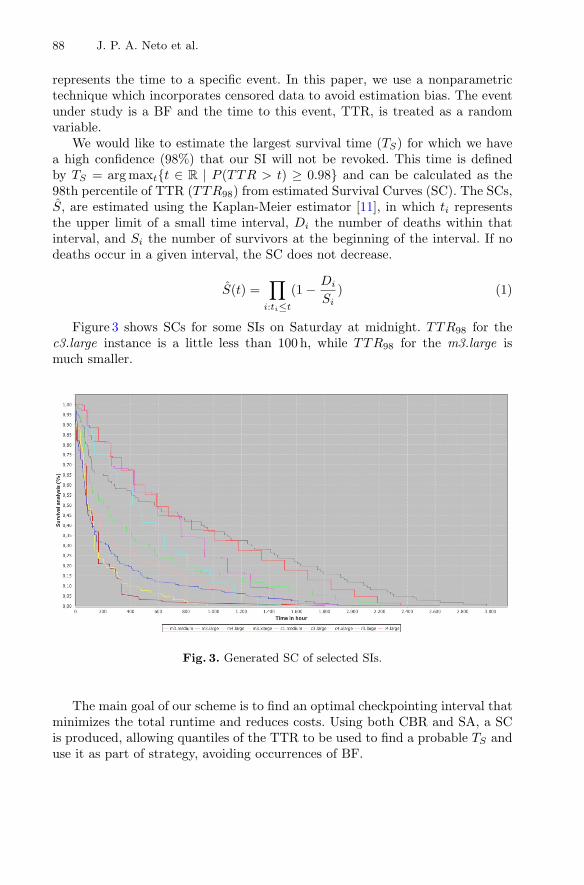
88 J. P. A. Neto et al.
represents the time to a specific event. In this paper, we use a nonparametrictechnique which incorporates censored data to avoid estimation bias. The eventunder study is a BF and the time to this event, TTR, is treated as a randomvariable.
We would like to estimate the largest survival time (TS) for which we havea high confidence (98%) that our SI will not be revoked. This time is definedby TS = arg maxt{t ∈ R | P (TTR > t) ≥ 0.98} and can be calculated as the98th percentile of TTR (TTR98) from estimated Survival Curves (SC). The SCs,S, are estimated using the Kaplan-Meier estimator [11], in which ti representsthe upper limit of a small time interval, Di the number of deaths within thatinterval, and Si the number of survivors at the beginning of the interval. If nodeaths occur in a given interval, the SC does not decrease.
S(t) =∏
i:ti≤t
(1 − Di
Si) (1)
Figure 3 shows SCs for some SIs on Saturday at midnight. TTR98 for thec3.large instance is a little less than 100 h, while TTR98 for the m3.large ismuch smaller.
Fig. 3. Generated SC of selected SIs.
The main goal of our scheme is to find an optimal checkpointing interval thatminimizes the total runtime and reduces costs. Using both CBR and SA, a SCis produced, allowing quantiles of the TTR to be used to find a probable TS anduse it as part of strategy, avoiding occurrences of BF.

A Prediction Approach to Define Checkpoint Intervals in Spot Instances 89
4 Experimental Evaluation
We evaluate our proposed checkpointing scheme for 37 SIs in all zones of theUS-WEST region. Using 6 months of real price changes, collected from Aprilto December of 2017, our experiment simulates 389.576 scenarios with Ubid =Estbid(Pt, n) | n ∈ N = {1 . . . 7}, using all combinations of days and hours forthe 13 weeks in October, November and December.
From the collected data, approximately 1 million cases were generated.Figure 4 shows a SC generated by the experiments. The value of TTR98 is indi-cated. We then repeated the same experiment, varying n in the Estbid functionbetween 1 and 7 days. Our results show that n = 7 is the best strategy, with allothers performing worse.
Fig. 4. SC of c1.medium on Sunday at 5am.
Each DOW and HID relationship has its own SC and a set of SC quantilescan be represented as a Survival Time Matrix (STM), as illustrated in Table 1,which shows TTR98 times, in minutes, obtained by 98th confidence level.
Table 1. Generated STM of c1.medium SI.
0 1 2 3 4 5 6 7 8 9 10 11 12 13 14 15 16 17 18 19 20 21 22 23
1 95 129 76 220 142 100 86 130 75 706 636 569 201 168 119 330 270 208 150 90 65 151 117 94
2 83 134 78 221 159 102 84 107 68 134 123 173 129 93 68 118 95 167 109 75 69 210 121 101
3 103 129 73 226 143 100 63 154 80 445 360 309 132 189 223 156 250 192 133 74 66 345 142 101
4 108 136 80 138 111 90 199 172 79 124 360 300 215 149 102 61 261 199 141 81 68 361 194 154
5 173 138 87 119 73 102 69 128 80 717 634 574 461 438 372 318 249 191 138 85 63 227 160 128
6 85 70 69 198 134 81 67 128 78 591 253 471 169 109 123 231 189 130 89 93 64 84 80 70
7 73 120 60 207 114 99 77 134 74 680 575 346 120 111 220 238 210 164 116 89 67 130 77 120

90 J. P. A. Neto et al.
To evaluate STM times, a set of experiments that compare STM values withreal scenarios was created. Using the same experimental scenario, 80.808 simu-lations were executed. An example of the c1.medium instance is illustrated inFig. 5. Very good results can be seen, with mean success rates around 80% withstandard deviation of 1.36% points.
Fig. 5. Heat map of survival success compared of TTR times in c1.medium instance.
An unsecured gap can be observed on Monday and Tuesday between 1am and10am, with 8 failures in 13 attempts, showing that another bid strategy is neededto increase the observed TTR and achieve better success rates. Considering all37 instances’ simulations, the success rate goes up to around 94%. This occursbecause instances with expensive price values have stable variations, allowinglong TTR times.
To achieve better results, a new strategy can be incorporated into the Sfunction, where more recent results receive a greater weight. In this strategy, thetime interval used in our experiment was reduced to 5 months, from April toAugust of 2017. With this change, a new STM was generated, creating a newmatrix that represents the survival times over this period (MTS′).
Then, a new matrix that represents only September of 2017 was generated(MTS′′) and a new STM was calculated as the median of MTS′ and MTS′′ . Theresults of this calculation are presented in Table 2.
Table 2. A new STM created after recency strategy in S function.
0 1 2 3 4 5 6 7 8 9 10 11 12 13 14 15 16 17 18 19 20 21 22 23
1 263 203143 83 1251 1191 1176 1090 1042 970 891 831 460 723 670 610 576 694 636 576 514 456 395 315
2 280 569349 256 404 363 313 255 195 135 92 276 215 155 96 71 585 524 465 402 344 284 233 173
3 114 338348 309 253 193 157 159 119 80 888 820 664 700 649 794 756 674 614 588 516 480 420 353
4 343 304224 184 215 175 117 167 158 100 192 390 333 295 238 245 187 130 74 62 394 334 297 223
5 163 184247 195 500 472 425 434 374 314 182 117 188 133 126 742 687 627 572 512 447 387 599 539
6 461 293223 323 238 206 172 252 410 350 317 415 355 276 235 192 135 284 424 364 300 252 188 128
7 109 619558 498 446 391 333 289 229 159 113 800 494 685 852 795 735 680 612 555 500 438 378 318
Better results were achieved with this change and can be observed in Fig. 6.Giving greater weight to more recent results allowed a gain of 8%, reaching an88% success rate under the same conditions of our experiment. The new resultsfor the DOW and HID relationship can be observed in Fig. 6.
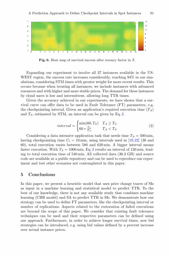
A Prediction Approach to Define Checkpoint Intervals in Spot Instances 91
Fig. 6. Heat map of survival success after recency factor in S.
Expanding our experiment to involve all 37 instances available in the US-WEST region, the success rate increases considerably, reaching 94% in our sim-ulations, considering STM times with greater weight for more recent results. Thisoccurs because when treating all instances, we include instances with advancedresources and with higher and more stable prices. The demand for these instancesby cloud users is low and intermittent, allowing long TTR times.
Given the accuracy achieved in our experiments, we have shown that a sur-vival curve can offer data to be used in Fault Tolerance (FT) parameters, e.g.the checkpointing interval. Given an application’s required execution time (TA)and TS , estimated by STM, an interval can be given by Eq. 2.
interval =
{min(60, TS) TA ≥ TS
60 ∗ TS
TATA < TS
(2)
Considering a data intensive application task that needs time TA = 500 min,having checkpointing time Ct = 10 min, using intervals used in [19,22] (30 and60), total execution varies between 580 and 620 min. A bigger interval meansfaster execution. With TS = 1000 min, Eq. 2 results an interval of 120 min, lead-ing to total execution time of 540 min. All collected data (30.3 GB) and sourcecode are available at a public repository and can be used to reproduce our exper-iment and test other scenarios not contemplated in this paper.
5 Conclusions
In this paper, we present a heuristic model that uses price change traces of SIsas input in a machine learning and statistical model to predict TTR. To thebest of our knowledge, there is not any available study that combines machinelearning (CBR model) and SA to predict TTR in SIs. We demonstrate how ourstrategy can be used to define FT parameters, like the checkpointing interval ornumber of replications. Aspects related to the restoration of failed executionsare beyond the scope of this paper. We consider that existing fault tolerancetechniques can be used and their respective parameters can be defined usingour approach. Furthermore, in order to achieve longer survival times, new bidstrategies can be introduced, e.g. using bid values defined by a percent increaseover actual instance prices.

92 J. P. A. Neto et al.
The performed simulations have confirmed the efficiency and the accuracyof the proposed model when used in a real environment with real data. Betterresults are achieved when strategies which place more weight on recent data areexplored. Future work can explore other strategies to exploit more recent data,such as comparing recent instance price changes with previously establishedchange patterns to update FT parameters, like checkpoint intervals. Use of theproposed strategy to definite the checkpoint interval decreases the total time ofexecution, allowing more effective use of SIs and reducing monetary costs forcloud users.
References
1. Aamodt, A., Plaza, E.: Case-based reasoning: foundational issues, methodologicalvariations, and system approaches. AI Commun. 7(1), 39–59 (1994)
2. Buyya, R., Yeo, C.S., Venugopal, S., Broberg, J., Brandic, I.: Cloud computingand emerging IT platforms: vision, hype, and reality for delivering computing asthe 5th utility. Future Gener. Comput. Syst. 25(6), 599–616 (2009)
3. Elnozahy, E.N.(M.), Alvisi, L., Wang, Y.-M., Johnson, D.B.: A survey of rollback-recovery protocols in message-passing systems. ACM Comput. Surv. 34(3), 375–408 (2002). https://doi.org/10.1145/568522.568525. ISSN 0360-0300
4. He, X., Shenoy, P., Sitaraman, R., Irwin, D.: Cutting the cost of hosting onlineservices using cloud spot markets. In: Proceedings of the 24th International Sym-posium on High-Performance Parallel and Distributed Computing - HPDC 2015,pp. 207–218. ACN Press, New York (2015)
5. Huang, K., Gao, X., Zhang, F., Xiao, J.: COMS: customer oriented migration ser-vice. In: 2017 IEEE 10th International Conference on Cloud Computing (CLOUD),pp. 692–695. IEEE, June 2017
6. Jangjaimon, I., Tzeng, N.-F.: Effective cost reduction for elastic clouds under spotinstance pricing through adaptive checkpointing. IEEE Trans. Comput. 64(2), 396–409 (2015)
7. Javadi, B., Thulasiram, R.K., Buyya, R.: Characterizing spot price dynamics inpublic cloud environments. Future Gener. Comput. Syst. 29(4), 988–999 (2013)
8. Javadi, D., Thulasiramy, R.K., Buyya, R.: Statistical modeling of spot instanceprices in public cloud environments. In: 2011 Fourth IEEE International Conferenceon Utility and Cloud Computing, pp. 219–228. IEEE, December 2011
9. Khandelwal, V., Chaturvedi, A., Gupta, C.P.: Amazon EC2 spot price predictionusing regression random forests. IEEE Trans. Cloud Comput. 7161(c), 1 (2017)
10. Lee, K., Son, M.: DeepSpotCloud: leveraging cross-region GPU spot instances fordeep learning. In: 2017 IEEE 10th International Conference on Cloud Computing(CLOUD), pp. 98–105. IEEE, June 2017
11. Meeker, W.: Statistical Methods for Reliability Data. Wiley, New York (1998)12. Miller Jr., R.G.: Survival Analysis, vol. 66. Wiley, Hoboken (2011)13. Rappa, M.A.: The utility business model and the future of computing services.
IBM Syst. J. 43(1), 32–42 (2004)14. Amazon Web Services: Amazon EC2 spot instances. https://aws.amazon.com/ec2/
spot. Accessed Jan 201815. Sharma, P., Irwin, D., Shenoy, P.: Portfolio-driven resource management for tran-
sient cloud servers. Proc. ACM Meas. Anal. Comput. Syst. 1(1), 5:1–5:23 (2017)
A Prediction Approach to Define Checkpoint Intervals in Spot Instances 93
16. Sharma, P., Lee, S., Guo, T., Irwin, D., Shenoy, P.: SpotCheck: designing a deriva-tive IaaS cloud on the spot market. In: Proceedings of the Tenth European Con-ference on Computer Systems - EuroSys 2015, pp. 1–15 (2015)
17. Sharma, P., Lee, S., Guo, T., Irwin, D., Shenoy, P.: Managing risk in a derivativeIaaS cloud. IEEE Trans. Parallel Distrib. Syst. 9219(c), 1 (2017)
18. Shastri, S., Rizk, A., Irwin, D.: Transient guarantees: maximizing the value of idlecloud capacity. In: SC16: International Conference for High Performance Comput-ing, Networking, Storage and Analysis, pp. 992–1002. IEEE, November 2016
19. Voorsluys, W., Buyya, R.: Reliable provisioning of spot instances for compute-intensive applications. In: 2012 IEEE 26th International Conference on AdvancedInformation Networking and Applications, pp. 542–549. IEEE, March 2012
20. Voorsluys, W., Garg, S.K., Buyya, R.: Provisioning spot market cloud resourcesto create cost-effective virtual clusters. In: Xiang, Y., Cuzzocrea, A., Hobbs, M.,Zhou, W. (eds.) ICA3PP 2011 Part I. LNCS, vol. 7016, pp. 395–408. Springer,Heidelberg (2011). https://doi.org/10.1007/978-3-642-24650-0 34
21. Yi, S., Andrzejak, A., Kondo, D.: Monetary cost-aware checkpointing and migra-tion on amazon cloud spot instances. IEEE Trans. Serv. Comput. 5(4), 512–524(2012)
22. Zhou, J., Zhang, Y., Wong, W.-F.: Fault tolerant stencil computation on cloud-based GPU spot instances. IEEE Trans. Cloud Comput. 7161(c), 1 (2017)

Research Track: Cloud Container

Cloud Service Brokerage and ServiceArbitrage for Container-Based Cloud
Services
Ruediger Schulze(B)
IBM Germany Research and Development GmbH,Schoenaicher Str. 220, 71034 Boeblingen, Germany
Abstract. By exploiting the portability of application containers,platform- and software-as-a-service providers receive the flexibility todeploy and move their cloud services across infrastructure services deliv-ered by different providers. The aim of this research is to apply the con-cepts of cloud service brokerage to container-based cloud services andto define a method for service arbitrage in an environment with multi-ple infrastructure-as-a-service (IaaS) providers. A new placement methodbased on constraint programming is introduced for the optimised deploy-ment of containers across multiple IaaS providers. The benefits and lim-itations of the proposed method are discussed and the efficiency of themethod is evaluated based on multiple deployment scenarios.
1 Introduction
Container-based applications are on the rise. Docker [1] as an open platform forapplication containers has become very popular since its first release in June2014 and a complete ecosystem of supporting tools has grown up. With Docker,developers receive the option to package applications and their dependencies intoself-contained images that can run as containers on any server. Multiple largeCloud Service Providers (CSP) have embraced Docker as container technologyand announced alliances with the Docker company. Container-based applicationsare highly portable and independent of the hosting provider and hardware.
Cloud services such as Platform-as-a-services (PaaS) and Software-as-a-services (SaaS) have usually a topology that aligns with the components of amulti-tier architecture, including tiers for presentation, business logic and dataaccess. The topology of the cloud service describes the structure of the IT ser-vice delivered by the CSP, the components of the service and the relationshipsbetween them. Cloud services designed for the use in enterprises have multipleQuality of Service (QoS) requirements such as High Availability (HA) and Disas-ter Recovery (DR) targets, performance and scalability requirements, and requirecompliance to security standards and data location regulations. The require-ments for HA, DR and horizontal scaling are the drivers to design and deploy
c© Springer International Publishing AG, part of Springer Nature 2018M. Luo and L.-J. Zhang (Eds.): CLOUD 2018, LNCS 10967, pp. 97–111, 2018.https://doi.org/10.1007/978-3-319-94295-7_7

98 R. Schulze
the cloud services in multi-node topologies which may span multiple availabilityzones and geographical sites.
PaaS and SaaS providers in public or private cloud environments receive withDocker the option to deliver their cloud services using container-based applica-tions or micro-services. The portability of the application containers enablesthem to easily move cloud services between IaaS providers and to locationswhere, for instance, the customer’s data resides, the best SLA is achieved orwhere the hosting is most cost-effective. PaaS and SaaS providers will benefitfrom employing brokerage services that allow them to choose from a varietyof IaaS providers and to optimise the deployment of their cloud services withrespect to the QoS requirements, distribution and cost. By using a Cloud Ser-vice Broker (CSB), PaaS and SaaS providers will be enabled to structure theiroffering portfolio with additional flexibility and to quickly respond to new orchanging customer requirements. New options arise from the easy deploymentof the containers across the multiple IaaS providers. A PaaS or SaaS providermay deploy a container to a new geographic location by selecting a different IaaSprovider when the primary one is not available there. A globally delivered cloudservice may be provided by using resources from multiple IaaS providers. DRuse cases may be realized by selecting a different provider for the backup site.Load-balancing and scalability built into the cloud service will allow to gradu-ally migrating the service from one provider to another one with no downtimeby simply moving the containers to the new provider.
Cloud service brokerage for application containers requires to define a newmethod for the optimised placement of the containers on IaaS resources of mul-tiple providers. The method has to take the attributes of the containers andthe IaaS resources into account, and honour the QoS requirements of enterprise-ready cloud services. The initial placement of the containers has to follow thespecification of the topology of the cloud service. Aside of the attributes used forrating IaaS providers, the CSB has to consider container related attributes suchas the built-in container support of the IaaS providers, the packaging of con-tainers in virtual machines and the clustering of containers. The optimisationof the infrastructure resources of the container-based cloud services has to bewithout impact and visibility to the cloud service consumers. Access to user dataand network connectivity to the cloud services have to be handled and delivereduninterrupted, and without the need to reconfigure clients.
A CSB for application containers may use a constraint programming-basedengine to make the placement decision about the optimal IaaS provider. Theengine will use as input the requirements of the container and information abouteach of the available IaaS providers. The objective of this research is to definea method for service arbitrage that allows for the optimised placement of con-tainers in a cloud environment with multiple IaaS providers and to demonstratethe feasibility of the proposed method.

Cloud Service Brokerage and Service Arbitrage 99
2 Background Research
2.1 Cloud Service Broker
The definition of a cloud broker as introduced by NIST is widely referenced byother authors, e.g., in [2–5]. In the NIST CCRA [6], a cloud broker is describedas an “entity that manages the use, performance and delivery of cloud servicesand negotiates relationships between cloud providers and cloud consumers.” Thecloud broker is an organisation that serves as a third-party entity as a centralisedcoordinator of cloud services for other organisations and enables users to inter-act through a single interface with multiple service providers [2,7]. Gartner [8]describes cloud service brokerage as “an IT role and business model in whicha company or other entity adds value to one or more (public or private) cloudservices on behalf of one or more consumers of that service via three primaryroles including aggregation, integration and customisation brokerage.”
NIST [6] and Gartner [9] define three categories of services that can be pro-vided by a CSB. Service intermediation enables a CSB to enhance a service byimproving some specific capability and providing value-added services to cloudconsumers. Service intermediation is responsible for service access and iden-tity management, performance reporting, enhanced security, service pricing andbilling. A CSB uses service aggregation to combine and integrate multiple ser-vices into one or more new services while ensuring interoperability. The CSB isresponsible for the integration and consolidation of data across multiple serviceproviders, and ensures the secure movement of the data between the cloud con-sumer and the cloud providers. The key aspect of the service aggregation is toease service selection and present services from separate providers as a uniqueset of services to the cloud service consumer. Service arbitrage is the process ofdetermining the best CSP. The CSB has the flexibility to choose a service frommultiple providers and can, for example, use a credit-scoring service to measureand select a provider with the best score. Service arbitrage adds flexibility andchoice to service aggregation as the aggregated services are not fixed.
Six key attributes of CSB are derived in [7] mainly based on the categoriesdefined by NIST [6] and Gartner [8,9], and used for evaluation of existing CSBs:intermediation, aggregation, arbitrage, customisation, integration and standard-isation. According to [10], integration is focused on creating an unified, com-mon system of services by integrating private and public clouds or bridgingbetween CSPs. Customisation refers to the aggregation and integration withother value-added services, including the creation of new original services [10].Both integration and customisation are closely interlinked with service aggrega-tion and intermediation, and in-fact it is difficult to find distinct definitions ofthese attributes in the literature. Standardisation among the CSB mechanismsand across the cloud services of different providers enables interoperability, andsupports the process of service selection by a CSB.
A comprehensive model of a CSB architecture is described in [2]. The CSBenvironment is built of the same components as the management platform fora single cloud but additional complexity is introduced into the system by the
100 R. Schulze
requirement to support multiple CSPs. Bond [2] distinguishes between the func-tions of the Cloud Broker Portal, the Cloud Broker Operations and Managementand the multiple CSPs, and aligns them in a layered model of a vendor-agnosticCSB architecture. Governance is introduced in addition as a set of functionswhich are orthogonal to the layers of the model and have to be realised for allfunctional components of the architecture.
A taxonomy of brokering mechanisms is given in [12]. Externally managedbrokers are provided off-premise by a centralized entity, for instance, by a third-party cloud provider or SaaS offering. Externally managed brokers are transpar-ent for applications using the services provided by the broker. Directly managedbrokers are incorporated into an application, have to keep track of the appli-cation’s performance and be built to meet the availability and dependabilityrequirements of the applications. Externally managed brokers can be classifiedinto SLA-based and trigger-action brokers. In case of SLA-based broker, a clouduser specifies the brokering requirements of a SLA in form of constraints andobjectives, and the CSB finds the most suitable cloud service by taking intoaccount the user requirements specified by the SLA. For trigger-action broker,a cloud user specifies a set of triggers and associates actions with them. A trig-ger becomes active when a predefined condition is meet, e.g., the threshold of aspecific metric is exceeded, and the associated action is executed. Actions canbe, for instance, scale-out and provisioning activities, and may include burstinginto a public cloud when there is a spike in the demand for computing capacity.
In the context of the interoperability of clouds, the following challenges aredescribed in [13] and applied here to CSBs. In an environment with multiplecloud service providers, each provider is expected to have its own SLA man-agement mechanism. A CSB has to establish federation of the SLAs from eachCSP in order to set up and enforce a global SLA. Methods and protocols forthe negotiation of dynamic and flexible SLAs between the CSB and the multipleCSPs are required. Another important issue is the enforcement of the SLAs inenvironments with conflicting policies and goals, e.g., a CSB may offer a ser-vice with a SLA for HA, while none of the providers are willing to offer sucha service. In addition to the SLA, there can be a Federation-Level Agreementthat defines rules and conditions between the CSB and the CSPs, e.g., aboutpools of resources and the QoS such as the minimum expected availability. TheCSB has to establish functions for matching the guaranteed QoS of cloud ser-vices offered by the CSPs with the QoS requirements of the end-user, and formonitoring that the promised QoS and SLA is provided to the cloud serviceconsumer. The dependencies of a CSP to other providers have to be consideredby the CSB as well. The QoS of a higher-layered service can be affected in caseswhen the CSP of the service itself uses external services. If one of the providersof the lower-layered services is not functioning properly, the performance of thehigher-layered service may be affected and impact finally the SLA agreed by theCSB. The CSB has to guarantee the security, confidentiality and privacy of thedata processed by the services provided. Within the country where the servicesare delivered, the CSB must comply with the legislation and laws concerning

Cloud Service Brokerage and Service Arbitrage 101
the privacy and security of the data. Therefore, the CSB has to implement geo-location and legislation awareness policies and enforce compliance with thosepolicies. As part of the SLA management, services of specific providers can beavoided or agreement can be made that placing data outside of a given countryis prohibited.
The results of a survey of CSB projects are described in [14]. The authorsconsider four categories of CSB technologies: CSBs for performance to addressissues of cloud performance comparison and prediction, CSBs for applicationmigration which provide decision support when moving applications to the cloud,theoretical models for CSBs which describe purely theoretical and mathematicaltechniques and data for CSBs that summarises providers of data and metricsavailable for use by CSBs. A comprehensive list of commercial CSB projectsis given in [10]. Recent research about CSBs has a significant focus on servicearbitration across numerous CSPs, in particular on optimising the allocation ofresources from different IaaS providers. The use of arbitration engines enablesCSBs to automatically determine the best CSP and service for any given cus-tomer order. The attributes considered in the optimisation process vary depend-ing on the proposed method. Typically attributes for rating IaaS providers are:the supported operating systems and configurations, geographical location, costsand rates, bandwidth and performance, SLA terms, legalisation and security,compliance and audit [15,16].
The placement of VMs in cloud and virtual environments is a critical opera-tion as it has an direct impact on the performance, resource utilisation, power-consumption and cost. The subject of VM placement is widely discussed in theresearch literature. Detailed reviews of the current VM placement algorithms canbe found in [17,18]. According to [18], the mono-objective, multi-objective solvedas mono-objective and pure multi-objective approaches can be distinguished withrespective optimisation objectives. Mono-objective methods are designed for theoptimisation of a single objective or the individual optimisation of more objec-tive functions, but one at a time. For multi-objective solved as mono-objectiveapproaches, multiple objective functions are combined into a single objectivefunction. The weighted sum method is used most often by this approach. Thismethod defines one objective function as the linear combination of multipleobjectives. A disadvantage of this approach is that it requires knowledge aboutthe correct combination of the objective functions – which is not always avail-able. Pure multi-objective approaches have a vector of multiple objective func-tions that are optimised. Only a small number of methods are described in theliterature which use a pure multi-objective approach for VM placement.
A broad range of different VM placement schemes (18 different in total)are analysed in [17]. Constraint programming based VM placement is describedas one of the considered placement schemes. The following classification of theplacement schemes is proposed: Resource-aware VM placement schemes con-sider the infrastructure resource requirements of the VMs are considered in theplacement decisions by these schemes. Efficient resource-aware placement triesto optimally place VMs on the hosts, so that the overall resource utilisation
102 R. Schulze
is maximised. Most of the schemes consider CPU and memory resources, somenetwork resources, and a minor number includes the device or disk I/O, or try tominimise the number of active hosts. Designed for the use by the CSPs, power-aware VM placement schemes try to make cloud data centres more efficient andto reduce the power consumption in order to enable green cloud computing. Theobjective of these schemes is to reduce the number of active host, networkingand other data center components. The methods include VM consolidation andpackaging of VMs on the same host or in the same rack, and powering off notneeded VMs, hosts and network components. The attributes considered by thepower-aware schemes include the CPU utilisation (e.g., based on the states: idle,average, active and over utilised), the server power usage and the host status(running, ready, sleep, off), costs for network routing and data center powerusage, and the distance between VMs. Network-aware VM placement schemestry to reduce the network traffic or try to distribute network traffic evenly inorder avoid congestion. The placement schemes allocate the VMs with moreor extensive communication on the same host, to the same switch and rack, orwithin the same data center in order to reduce the network traffic within the datacenter and across data centres. Most common is the consideration of the trafficbetween VMs by the network-aware VM placement schemes, some evaluate thetraffic between the hosts and selected schemes try to minimise the transfer timebetween the VMs and data, and the distance between the VMs. Cost-aware VMplacement schemes try to reduce the costs for the CSPs while considering theQoS of the cloud services and honouring the SLAs. The schemes use differenttypes of costs as attributes, such as the VM, physical machine, cooling and datacenter costs, and the distance between the VMs and the clients.
Conceptually a similar approach is taken in [18] with the classification ofthe objective functions. Based on the study of 56 different objective functions,the classification into five groups of objective functions is described: EnergyConsumption Minimisation, Network Traffic Minimisation, Economical CostsOptimisation, Performance Maximisation and Resource Utilisation Maximisa-tion. Most of the publications are focused on single-cloud environments, i.e. foruse by CSPs. Seven of the methods are suitable for multi-cloud environments,i.e. use multiple cloud computing data centres from one or more CSP. Only twoarticles take a broker-oriented approach.
Different methods are employed by CSBs for rating IaaS providers, e.g.,genetics algorithms [19,20] and rough sets [16,21]. Multiple projects proposeCSBs which take advantage of the different price options such as for on-demand, reservation and spot instances [22], examples can be found in [23–26].There are a couple of academic and open-source implementations of CSBs, e.g.,STRATOS [27], QBROKAGE [19] and CompatibleOne [28].
2.2 Constraint Programming
Constraint programming is a form of declarative programming which uses vari-ables and their domains, constraints and objective functions in order to solve

Cloud Service Brokerage and Service Arbitrage 103
a given problem. The purpose of constraint programming is to solve constraintsatisfaction problems as defined in [30,31]:
Definition 1 (Constraint Satisfaction Problem). A Constraint Satisfac-tion Problem P is a triple P = (X,D,C) where X is an n-tuple of variables X =(x1, x2, . . . , xn), D is a corresponding n-tuple of domains D = (D1,D2, . . . , Dn)such that xi ∈ Di, C is a t-tuple of constraints C = (C1, C2, . . . , Ct).
The domain Di of a variable xi is a finite set of numbers, and can be continuousor of a discrete set of values. In order to describe a constraint satisfaction problemP, a finite sequence of variables with their respective domains is used togetherwith a finite set of constraints. A constraint over a sequence of variables is asubset of the Cartesian product of the variables’ domains in the scope of theconstraint.
Definition 2 (Constraints). C = (C1, C2, . . . , Ct) is the set of constraints.A constraint Cj is a pair
(RSj
, Sj
)where RSj
is a relation on the variablesin Sj = scope(Cj), i.e. the relation RSj
is a subset of the Cartesian productD1 × . . . × Dm of the domains D1,D2, . . . , Dm for the variables in Sj.
A solution of the Constraint Satisfaction Problem P is defined as follows:
Definition 3 (Solution of P). A solution to the Constraint Satisfaction Prob-lem P is a n-tuple A = (a1, a2, . . . , an) where ai ∈ Di and each Cj is satisfiedin that RSj
holds the projection of A onto the scope of Sj.
The definition of multiple global constraints such as the alldifferent constraintis described in the literature. The constraint alldifferent requires that thevariables x1,2 , . . . , xn take all different values. An overview of the most popularglobal constraints is given in [32].
Several publications focus on the use of CP-based cloud selection and VMplacement methods. A method for cloud service match making based on QoSdemand is introduced in [33]. CP is a convenient method for optimising theplacement of VMs, as placement constraints can be directly expressed by vari-ables representing the assignment of the VMs to the hosts and the allocationof resources for the VMs placed on each host. Resource-aware VM placementschemes are presented in [34–36]. A combined CP and heuristic algorithm isutilised in [35]. Special focus is put on fault tolerance and HA in [36]. In [37],the CP-based, open source VM scheduler BtrPlace [38] is used to exhibit SLAviolations for discrete placement constraints, as these do not consider interimsstates of a reconfiguration process. As consequence, BtrPlace is extended with apreliminary version of continuous constraints and it is proved that these removethe temporary violation and improve the reliability. Power-aware methods arediscussed in [39,40].
3 Method for Service Arbitrage
Aims of this research is to define a method for optimising the deployment ofcontainer-based applications across different CSPs. The objective is to find for

104 R. Schulze
a given Docker container c the optimal host h. A host h is a virtual or physicalmachine that meets the requirements of the container c and is delivered byan IaaS provider. The optimisation problem to be solved can be described astransformation of a container domain C into a host domain H:
f : C → H, c �→ h, where c ∈ C and h ∈ H. (1)
The requirements of a container c are expressed as vector rc = (rc,1, rc,i . . . , rc,n).Each attribute rc,i is an element or subset of a domain Ri with a finite numberof elements. Likewise, the attributes of a host h are described by the a vectorah = (ah,1, ah,j , . . . , ah,m) for which each attribute ah,j belongs to a domainAj and A = (A1, Aj , . . . , Am). In order to solve the optimisation problem, therequirements rc,i of the containers and the attributes ah,j of the hosts have tobe considered. As method for finding the optimal host h for a given containerc, a CP model is used. As per Definition 1, a constraint satisfaction problemP is defined as the triple P = (X,D,C). The objective of the CP model is toprovide solutions for the container placement problem Pplacement. The variablesX and the corresponding domains D of the problem Pplacement are defined bythe attribute domains A of the hosts H, i.e. D = A and X = (a1, aj , . . . , am)where aj ∈ Aj . Provided that the function index returns the index set I of anygiven set S, so that
index : S → I, si �→ i = index(s), (2)
then can be defined for the variables and domains of the host attributes thefollowing:
provider : a1 ∈ A1 and A1 = index(P) where (3)P = {AWS,DigitalOcean,Azure,SoftLayer,Packet}
host type : a2 ∈ A2 and A2 = index(T) where (4)T = {physical, virtual}
region : a3 ∈ A3 and A3 = index(R) where (5)R = {Australia,Brazil,Canada,France,Germany}R = R ∪ {Great Britain,Hongkong, India, Ireland}R = R ∪ {Italy, Japan,Mexico,Netherlands, }R = R ∪ {Singapore,California, Iowa,New Jersey}R = R ∪ {New York,Oregon,Texas,Washington}R = R ∪ {Virginia} (6)

Cloud Service Brokerage and Service Arbitrage 105
data centres : a4 ∈ A4 and A4 = {1, .., 52} (7)availability zone : a5 ∈ A5 and A5 = {0, .., 5} (8)
cpu : a6 ∈ A6 and A6 = {1, .., 40} (9)memory (GB) : a7 ∈ A7 and A7 = {1, .., 488} (10)disk size (GB) : a8 ∈ A8 and A8 = {1, .., 48000} (11)
disk type : a9 ∈ A9 and A9 = index(D) where (12)D = {HDD,SSD}
private : a10 ∈ A10 and A10 = {0, 1} (13)optimised : a11 ∈ A11 and A11 = index(O) where (14)
O = {compute,memory, gpu, storage}O = O ∪ {network,none}
cost : a12 ∈ A12 and A12 = {1, .., 99999} (15)
In order to describe the constraints C, the requirements rc = (rc,1, rc,i . . . , rc,n)of a container c have to be detailed first. The properties ha scale and dr scaleare introduced to address the requirements for HA and DR. The requirementha scale describes how many containers have to be deployed across the datacentres or available zones within one region and dr scale is the number of con-tainers that have to be deployed across multiple regions of the same or multipleproviders in order to achieve protection against a disaster. The op factor rc,9allows to request a larger host which can run rc,9 instances of the container c.The price limit ($ 0.0001 per hour) specifies the maximum cost of host perhour which must not be exceeded. The attribute private rc,11 allows to requestto place the container c on a dedicated host.
host type : rc,1 ∈ R1 and R1 = A2 (16)region : rc,2 ∈ R2 and R2 = A3 (17)
cpu : rc,3 ∈ R3 and R3 = A6 (18)memory (GB) : rc,4 ∈ R4 and R4 = A7 (19)disk size (GB) : rc,5 ∈ R5 and R5 = A8 (20)
disk type : rc,6 ∈ R6 and R6 = A9 (21)ha scale : rc,7 ∈ R7 and R7 = {1, .., 5} (22)dr scale : rc,8 ∈ R8 and R8 = {1, .., 5} (23)
op factor : rc,9 ∈ R9 and R9 = {1, .., 10} (24)price limit : rc,10 ∈ R10 and R10 = A12 (25)
private : rc,11 ∈ R11 and R11 = A10 (26)optimized : rc,12 ∈ R12 and R12 = A11 (27)
image : rc,13 ∈ R13 and R13 = I where (28)I is the set of Docker images

106 R. Schulze
In order to allow the placement of a container c either on an existing host ora new host, the domain H to be searched is defined as the union of the hosttemplates T , i.e. the set of hosts which can be provisioned, and the alreadyprovisioned hosts H:
H = T ∪ H (29)
wherein T is the superset of the templates tp from all providers P:
T =⋃
p∈P
T p and tp ∈ T p (30)
The template tp is described by the attribute vector apt and domains Ap:
apt = (apt,1, apt,j , . . . , a
pt,m) and apt,j ∈ Ap
j (31)Ap = Ap
1, Apj , . . . , A
pm and p ∈ P (32)
The set of already provisioned hosts H is the union of the deployed hosts hp atall providers P:
H =⋃
p∈P
Hp and hp ∈ Hp (33)
Provided that the host hp is provisioned using the template hp and that Ch
denotes the set of containers deployed on the host h, the available resources onthe host hp can the be determined as follows:
cpu : ah,6 = apt,6 −∑
c∈Ch
rc,3 (34)
memory(GB) : ah,7 = apt,7 −∑
c∈Ch
rc,4 (35)
disksize(GB) : ah,8 = apt,8 −∑
c∈Ch
rc,5 (36)
cost : ah,12 =apt,12|Ch| (37)
The variables X represent the attributes of a single host. In order to respondto the requirements for HA and DR, multiple containers have to be placed on kanti-collocated hosts. Xe,f denotes the variables and ae,fj the attributes requiredto describe the k hosts he,f :
k =dr scale · ha scale (38)
Xe,f =(ae,f1 , ae,fj , . . . , ae,fm ) where ae,fj ∈ Aj (39)
1 ≤ e ≤ dr scale (40)1 ≤ f ≤ ha scale (41)
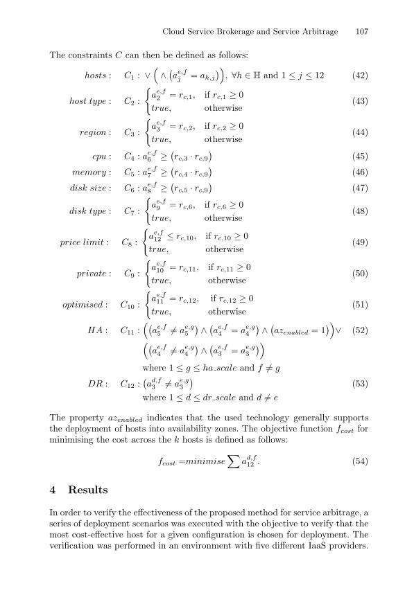
Cloud Service Brokerage and Service Arbitrage 107
The constraints C can then be defined as follows:
hosts : C1 : ∨(
∧ (ae,fj = ah,j
)), ∀h ∈ H and 1 ≤ j ≤ 12 (42)
host type : C2 :
{ae,f2 = rc,1, if rc,1 ≥ 0true, otherwise
(43)
region : C3 :
{ae,f3 = rc,2, if rc,2 ≥ 0true, otherwise
(44)
cpu : C4 : ae,f6 ≥ (rc,3 · rc,9
)(45)
memory : C5 : ae,f7 ≥ (rc,4 · rc,9
)(46)
disk size : C6 : ae,f8 ≥ (rc,5 · rc,9
)(47)
disk type : C7 :
{ae,f9 = rc,6, if rc,6 ≥ 0true, otherwise
(48)
price limit : C8 :
{ae,f12 ≤ rc,10, if rc,10 ≥ 0true, otherwise
(49)
private : C9 :
{ae,f10 = rc,11, if rc,11 ≥ 0true, otherwise
(50)
optimised : C10 :
{ae,f11 = rc,12, if rc,12 ≥ 0true, otherwise
(51)
HA : C11 :((
ae,f5 �= ae,g5
) ∧ (ae,f4 = ae,g4
) ∧ (azenabled = 1
))∨ (52)((
ae,f4 �= ae,g4
) ∧ (ae,f3 = ae,g3
))
where 1 ≤ g ≤ ha scale and f �= g
DR : C12 :(ad,f3 �= ae,g3
)(53)
where 1 ≤ d ≤ dr scale and d �= e
The property azenabled indicates that the used technology generally supportsthe deployment of hosts into availability zones. The objective function fcost forminimising the cost across the k hosts is defined as follows:
fcost =minimise∑
ad,f12 . (54)
4 Results
In order to verify the effectiveness of the proposed method for service arbitrage, aseries of deployment scenarios was executed with the objective to verify that themost cost-effective host for a given configuration is chosen for deployment. Theverification was performed in an environment with five different IaaS providers.

108 R. Schulze
In total, 3587 host templates with different server configurations in 22 regionsand 52 data centres were given to the CP model as input. Actual prices from theCSPs were used for each of the configurations. The CP model was implementedusing NumberJack [41] and the CP solver “Mistral” [42]. The execution of thetest scenarios showed that the used CP solver is able to find optimal solutionsfor the CP model. The CP solver returns solutions in a reasonable time whenonly a single container has to be placed. The runtime of the CP solver increasessignificantly when multiple containers have to placed across different locationsfor HA and DR. In this case, the number of variables and constraints suppliedto the CP model increase and the objective function becomes more complex. Inorder to validate if better performance results can be achieved with another CPsolver supported by NumberJack, the “MiniSat” solver [43] was used. The testexecution with “MiniSat” showed an increased CPU utilization on the hostingserver and significant longer runtime. All further tests were executed using the“Mistral” solver afterwards. By applying a lower price limit to a deploymentscenario with multiple containers, it was possible to obtain an optimal solutionquicker. With the price limit applied, the initial number of host templates canbe already reduced before the actual constraints are added to the CP model.The deployment scenarios with multiple containers shows as well that regionson different continents may be selected by the CP solver as optimal solution, e.g.Europe and North America. This solution may not be suitable for business usein all cases, e.g., when legal restrictions apply. Additional locality constraints oran objective function for minimising the distance between regions may be addedto the CP model in future.
5 Summary and Conclusions
An important aspects of the proposed CP model is that the emphasis is not onrating the CSPs but the particular hosts for their capability to run a specificcontainer, so that the CSP becomes only an attribute of the host. The proposedCP model was validated based on test data with host templates from five IaaSproviders, 22 regions and 52 data centres. In this experimental research it isshown that the proposed CP model is capable to find the optimal placementfor containers also in complex environments, and that HA and DR topologiesof applications can be realised. It is further shown that the CP solver “Mistral”[42] used by NumberJack runs stable for large CP models. The duration of theprocess for finding the optimal solution increases significantly when multiplecontainers have to placed across different locations for HA and DR. Hence, thepractical use of the proposed CP model in a production environment is notpossible. Further research is required to reduce the complexity inherited fromthe input attributes before the actual CP model is constructed. Other CP solversmay be evaluated and the integration of rule-based algorithms such as Rete [44]into the CSB framework can be investigated. The objective of the integrationwith a rule-based approach will be to limit the number of CP variables andconstraints to only the ones which are valid for a given request, so that the CP

Cloud Service Brokerage and Service Arbitrage 109
solver can find a solution to the objective function within a few seconds. Theadvantage of the combination of the two approaches will be that the rule-basedalgorithm can provide a reduction of the solution space, while the CP solver isstill used to find the best solution for the given objective function.
Aside of the runtime aspect, the CP model can be extended in future invarious ways. The CP model uses a mono-objective function to minimise thecost. A multi-objective approach may take additional performance attributesinto consideration and allow to maximise the service performance while provid-ing the most cost-effective price. Such performance attributes could be gath-ered from monitoring data of the containers during runtime or be collected fromIaaS benchmarking services like CloudHarmony [29]. The data model related theCP model is centred around host templates which represent virtual or physicalservers. CSPs offer compute, storage and network resources today as indepen-dent services with various, flexible options for selection. The CP model may beextended to allow for better consumption and distinction of those services inthe placement decisions. In addition, the CP model may be further extended tohonour region specific prices, and optionally to take price differences for reser-vation, on-demand and spot instances into account. Further extension of the CPmodel can be done to support node clusters with multiple nodes and serviceswith multiple containers.
With the proposed CP model, a first brokerage solution using service arbi-trage for containers is provided. The underlying concepts were successful verifiedand allow for future research and development in this area.
References
1. What is Docker? https://www.docker.com/what-docker2. Bond, J.: The Enterprise Cloud: Best Practices for Transforming Legacy IT.
O’Reilly Media Inc., Newton (2015)3. Amato, A., Di Martino, B., Venticinque, S.: Cloud brokering as a service. In: 2013
Eighth International Conference on P2P, Parallel, Grid, Cloud and Internet Com-puting (3PGCIC), pp. 9–16. IEEE (2013)
4. Park, J., An, Y., Yeom, K.: Virtual cloud bank: an architectural approach for inter-mediating cloud services. In: 2015 16th IEEE/ACIS International Conference onSoftware Engineering, Artificial Intelligence, Networking and Parallel/DistributedComputing (SNPD), pp. 1–6. IEEE (2015)
5. Khanna, P., Jain, S., Babu, B.: BroCUR: distributed cloud broker in a cloud feder-ation: brokerage peculiarities in a hybrid cloud. In: 2015 International Conferenceon Computing, Communication and Automation (ICCCA), pp. 729–734. IEEE(2015)
6. Liu, F., Tong, J., Mao, J., Bohn, R., Messina, J., Badger, L., Leaf, D.: NIST cloudcomputing reference architecture. NIST Spec. Publ. 500(2011), 292 (2011)
7. Mostajeran, E., Ismail, B.I., Khalid, M.F., Ong, H.: A survey on sla-based brokeringfor inter-cloud computing. In: 2015 Second International Conference on ComputingTechnology and Information Management (ICCTIM), pp. 25–31. IEEE (2015)
8. Gartner: Cloud service brokerage. Gartner Research (2016). http://www.gartner.com/it-glossary/cloud-services-brokerage-csb
110 R. Schulze
9. Gartner: Gartner says cloud consumers need brokerages to unlock the potential ofcloud services. Gartner Research, July 2009. http://www.gartner.com/newsroom/id/1064712
10. Guzek, M., Gniewek, A., Bouvry, P., Musial, J., Blazewicz, J.: Cloud brokering:current practices and upcoming challenges. IEEE Cloud Comput. 2, 40–47 (2015)
11. What is ITIL best practice? https://www.axelos.com/best-practice-solutions/itil/what-is-itil
12. Grozev, N., Buyya, R.: Inter-cloud architectures and application brokering: taxon-omy and survey. Softw. Pract. Exp. 44(3), 369–390 (2014)
13. Toosi, A.N., Calheiros, R.N., Buyya, R.: Interconnected cloud computing environ-ments: challenges, taxonomy, and survey. ACM Comput. Surv. (CSUR) 47(1), 7(2014)
14. Barker, A., Varghese, B., Thai, L.: Cloud services brokerage: a survey and researchroadmap. In: 2015 IEEE 8th International Conference on Cloud Computing(CLOUD), pp. 1029–1032. IEEE (2015)
15. Ngan, L.D., Tsai Flora, S., Keong, C.C., Kanagasabai, R.: Towards a commonbenchmark framework for cloud brokers. In: 2012 IEEE 18th International Confer-ence on Parallel and Distributed Systems (ICPADS), pp. 750–754. IEEE (2012)
16. Tiwari, A., Nagaraju, A., Mahrishi, M.: An optimized scheduling algorithm forcloud broker using adaptive cost model. In: 2013 IEEE 3rd International AdvanceComputing Conference (IACC), pp. 28–33. IEEE (2013)
17. Masdari, M., Nabavi, S.S., Ahmadi, V.: An overview of virtual machine placementschemes in cloud computing. J. Netw. Comput. Appl. 66, 106–127 (2016)
18. Lopez-Pires, F., Baran, B.: Virtual machine placement literature review. arXivpreprint arXiv:1506.01509 (2015)
19. Anastasi, G.F., Carlini, E., Coppola, M., Dazzi, P.: QBROKAGE: a genetic app-roach for QoS cloud brokering. In: 2014 IEEE 7th International Conference onCloud Computing (CLOUD), pp. 304–311. IEEE (2014)
20. Kessaci, Y., Melab, N., Talbi, E.-G.: A Pareto-based genetic algorithm for opti-mized assignment of VM requests on a cloud brokering environment. In: 2013 IEEECongress on Evolutionary Computation (CEC), pp. 2496–2503. IEEE (2013)
21. Srivastava, N.K., Singh, P., Singh, S.: Optimal adaptive CSP scheduling on basis ofpriority of specific service using cloud broker. In: 2014 9th International Conferenceon Industrial and Information Systems (ICIIS), pp. 1–6. IEEE (2014)
22. Amazon EC2 pricing. Amazon Web Services. https://aws.amazon.com/ec2/pricing/
23. Wang, W., Niu, D., Liang, B., Li, B.: Dynamic cloud instance acquisition via iaascloud brokerage. IEEE Trans. Parallel Distrib. Syst. 26(6), 1580–1593 (2015)
24. Liu, K., Peng, J., Liu, W., Yao, P., Huang, Z.: Dynamic resource reservation viabroker federation in cloud service: a fine-grained heuristic-based approach. In: 2014IEEE Global Communications Conference (GLOBECOM), pp. 2338–2343. IEEE(2014)
25. Nesmachnow, S., Iturriaga, S., Dorronsoro, B.: Efficient heuristics for profit opti-mization of virtual cloud brokers. IEEE Comput. Intell. Mag. 10(1), 33–43 (2015)
26. Vieira, C., Bittencourt, L., Madeira, E.: A scheduling strategy based on redun-dancy of service requests on iaas providers. In: 2015 23rd Euromicro InternationalConference on Parallel, Distributed and Network-Based Processing (PDP), pp.497–504. IEEE (2015)
27. Pawluk, P., Simmons, B., Smit, M., Litoiu, M., Mankovski, S.: IntroducingSTRATOS: a cloud broker service. In: 2012 IEEE Fifth International Conferenceon Cloud Computing, pp. 891–898. IEEE (2012)

Cloud Service Brokerage and Service Arbitrage 111
28. Yangui, S., Marshall, I.-J., Laisne, J.-P., Tata, S.: CompatibleOne: the open sourcecloud broker. J. Grid Comput. 12(1), 93–109 (2014)
29. Cloud Harmony - Transparency for the Cloud. Gartner, Inc. https://cloudharmony.com
30. Freuder, E.C., Mackworth, A.K.: Constraint satisfaction: an emerging paradigm.Handb. Constr. Program. 2, 13–27 (2006)
31. Apt, K.: Principles of Constraint Programming. Cambridge University Press, Cam-bridge (2003)
32. Bockmayr, A., Hooker, J.N.: Constraint programming. Handb. Oper. Res. Manag.Sci. 12, 559–600 (2005)
33. Zilci, B., Slawik, M., Kupper, A.: Cloud service matchmaking using constraint pro-gramming. In: 2015 IEEE 24th International Conference on Enabling Technologies:Infrastructure for Collaborative Enterprises (WETICE), pp. 63–68. IEEE (2015)
34. Zhang, L., Zhuang, Y., Zhu, W.: Constraint programming based virtual cloudresources allocation model. Int. J. Hybrid Inf. Technol. 6(6), 333–334 (2013)
35. Zhang, Y., Fu, X., Ramakrishnan, K.: Fine-grained multi-resource schedulingin cloud datacenters. In: 2014 IEEE 20th International Workshop on Local &Metropolitan Area Networks (LANMAN), pp. 1–6. IEEE (2014)
36. Bin, E., Biran, O., Boni, O., Hadad, E., Kolodner, E.K., Moatti, Y., Lorenz, D.H.:Guaranteeing high availability goals for virtual machine placement. In: 2011 31stInternational Conference on Distributed Computing Systems (ICDCS), pp. 700–709. IEEE (2011)
37. Dang, H.T., Hermenier, F.: Higher SLA satisfaction in datacenters with continuousVM placement constraints. In: Proceedings of the 9th Workshop on Hot Topics inDependable Systems, p. 1. ACM (2013)
38. BtrPlace - An Open-Source Flexible Virtual Machine Scheduler. http://www.btrplace.org
39. Van, H.N., Tran, F.D., Menaud, J.-M.: Performance and power management forcloud infrastructures. In: 2010 IEEE 3rd International Conference on Cloud Com-puting (CLOUD), pp. 329–336. IEEE (2010)
40. Dupont, C., Giuliani, G., Hermenier, F., Schulze, T., Somov, A.: An energy awareframework for virtual machine placement in cloud federated data centres. In: 2012Third International Conference on Future Energy Systems: Where Energy, Com-puting and Communication Meet (e-Energy), pp. 1–10. IEEE (2012)
41. NumberJack - A Python Contraint Programming platform. http://numberjack.ucc.ie
42. Mistral. http://homepages.laas.fr/ehebrard/mistral.html43. The MiniSat Page. http://minisat.se44. Forgy, C.L.: Rete: a fast algorithm for the many pattern/many object pattern
match problem. Artif. Intell. 19(1), 17–37 (1982)

Fault Injection and Detectionfor Artificial Intelligence Applications
in Container-Based Clouds
Kejiang Ye1(B), Yangyang Liu2, Guoyao Xu1,3, and Cheng-Zhong Xu1
1 Shenzhen Institutes of Advanced Technology,Chinese Academy of Sciences, Shenzhen, China
{kj.ye,cz.xu}@siat.ac.cn2 School of Computer Science and Technology, Xidian University, Xi’an, China
[email protected] Department of Electrical and Computer Engineering,
Wayne State University, Detroit, [email protected]
Abstract. Container technique is increasingly used to build moderncloud computing systems to achieve higher efficiency and lower resourcecosts, as compared with traditional virtual machine technique. Artifi-cial intelligence (AI) is a mainstream method to deal with big data,and is used in many areas to achieve better effectiveness. It is knownthat attacks happen every day in production cloud systems, however,the fault behaviors and interferences of up-to-date AI applications incontainer-based cloud systems is still not clear. This paper aims tostudy the reliability issue of container-based clouds. We first proposea fault injection framework for container-based cloud systems. We builda docker container environment installed with TensorFlow deep learningframework, and develop four typical attack programs, i.e., CPU attack,Memory attack, Disk attack and DDOS attack. Then, we inject theattack programs to the containers running AI applications (CNN, RNN,BRNN and DRNN), to observe fault behaviors and interferences phe-nomenon. After that, we design fault detection models based on quantileregression method to detect potential faults in containers. Experimentalresults show the proposed fault detection models can effectively detectthe injected faults with more than 60% Precision, more than 90% Recalland nearly 100% Accuracy.
1 Introduction
Container technology is experiencing a rapid development with the supportfrom industry like Google and Alibaba, and is being widely used in large scaleproduction environments [1,2]. Container technology is also called operating-system-level virtualization, which allows multiple isolated user-space instancessharing the same operating system kernel and applies CGroups to take controlof resources in the host. This provides functionality similar to a virtual machinec© Springer International Publishing AG, part of Springer Nature 2018M. Luo and L.-J. Zhang (Eds.): CLOUD 2018, LNCS 10967, pp. 112–127, 2018.https://doi.org/10.1007/978-3-319-94295-7_8

Fault Injection and Detection for AI Applications in Container-Based Clouds 113
(VM) but with a lighter footprint. While traditional virtualization solutions (e.g.,Hypervisor) need to interpose on various privileged operations (e.g., page-tablelookups) and use roundabout techniques to infer resource usage (e.g., balloon-ing). The result is that hypervisors are heavyweight, with slow boot times aswell as high run-time overheads.
Speedy launching time and tiny memory footprint are two outstanding fea-tures to make containers launch an application in less than a second and consumea very small amount of resources. Compared with virtual machines, adoptingcontainers not only improves the performance of applications, but also allowshosts to sustain more applications simultaneously [3]. So far, there have beena number of container products released to the market, such as LXC (LinuxContainer) [4], Docker [5], rkt (Rocket) [6], and OpenVZ [7], etc. Docker [5] is apopular runtime system for managing Linux containers, providing both manage-ment tools and a simple file format. Docker technology introduces lightweightvirtual machines on top of Linux containers called Docker containers. Majorcloud platforms include Amazon Web Service [8] and Google Compute Engine[9] are also beginning to provide public container services for developers to deployapplications in the cloud. Undoubtedly, the emergence of container technologyhas virtually changed the trend of cloud computing market.
Deep learning is a new area of machine learning research. It is the applicationto learning tasks of artificial neural networks (ANNs) that contain more thanone hidden layer. Deep learning is part of a broader family of machine learningmethods based on learning data representations, as opposed to task specific algo-rithms. Deep learning architectures such as deep neural networks, deep belief net-works and recurrent neural networks have been widely applied to fields includingcomputer vision, speech recognition, natural language processing, audio recogni-tion, social network filtering, machine translation and bioinformatics, where theyproduced results comparable to or in some cases superior to human experts. Ten-sorFlow [10] is an open source software library for numerical computation usingdata flow graphs. Nodes in the graph represent mathematical operations, whilethe graph edges represent the multidimensional data arrays (tensors) commu-nicated between them. TensorFlow was originally developed by researchers andengineers working on the Google Brain Team within Google’s Machine Intelli-gence research organization for the purposes of conducting machine learning anddeep neural networks research, but the system is general enough to be applicablein a wide variety of other domains as well.
There are already a lot of work focused on the performance issues of differ-ent applications running on containers [11–14]. However, the fault behavior andinterference of container-based cloud is still not clear. In fact, reliability is veryimportant and may cause serious consequences if faults are not timely handled,which not only hinders the runtime system, but also results in serious economiclosses. For example, on February 28th 2017, Amazon Web Services, the popularhosting and storage platform used by a huge range of companies, experienced S3service interruption for 4 hours in the Northern Virginia (US-EAST-1) Region,and then quickly spread other online service providers who rely on the S3 service[15]. This failure caused a large number of economic compensations for users. It is

114 K. Ye et al.
because cloud computing service providers usually set a Service Level Agreement(SLA) with customers. For example, when customers require 99.99% availability,it means that 99.99% of the time must meet the requirement for 365 days peryear. If the service breaks more than 0.01%, compensation is required.
Although reliability of cloud systems is important, it is not easy to solve thisproblem, mainly because: (1) Large scale. A typical data center involves morethan 100,000 servers and 10,000 switches, more nodes usually mean higher prob-ability of failure; (2) Complex application structure. Web search, e-commerce andother typical cloud programs have complex interactive behaviors. For example,an Amazon page request involves interactions with hundreds of components [16],error occurs in any one component will lead to anomalies of applications; (3)Diverse causes. Resource competition, resource bottlenecks, misconfiguration,defects of softwares, hardware failures and external attacks can cause anoma-lies or failures of cloud systems. Cloud systems are more prone to performanceanomalies than traditional platforms [17].
In this paper, we focus on the reliability issue of container-based cloud. Wefirst propose a fault injection framework for container-based cloud systems. Webuild a docker container environment installed with TensorFlow deep learningframework, and develop four typical attack programs, i.e., CPU attack, Memoryattack, Disk attack and DDOS attack. Then, we observe fault behaviors andinterferences phenomenon by injecting attack programs to the containers runningartificial intelligence (AI) applications (CNN, RNN, BRNN and DRNN). Wealso design fault detection models based on quantile regression method to detectpotential faults in containers.
Our main contributions are:
– We develop a fault injection tool as well as four typical attack programs forcontainer-based cloud systems. The fault programs include CPU attack, mem-ory attack, disk attack and network attack. The purpose of fault injection isto simulate abnormal behavior of containers.
– We investigate the fault behaviors and interferences between multiple con-tainers. We focus on four mainstream AI applications: Convolutional NeuralNetwork (CNN), Recurrent Neural Network (RNN), Bidirectional RecurrentNeural Network (BRN) and Dynamic Recurrent Neural Network (DRNN).
– We design fault detection models for container-based cloud systems. The mod-els are based on the quantile regression method. Part of the experimental datais used for training the models. Experimental results show that the proposedfault detection models can effectively detect the injected faults with morethan 60% Precision, more than 90% Recall and nearly 100% Accuracy.
2 Fault Injection Framework
2.1 Fault Injection Framework
AI Applications in Target Systems. Our fault injection framework is mainlydesigned for container-based cloud systems (see Fig. 1), but it would be easily
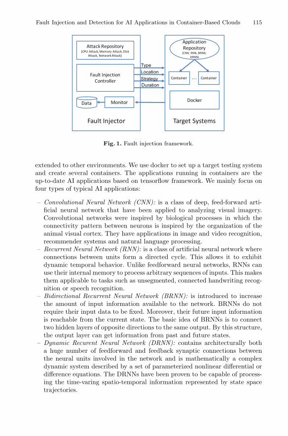
Fault Injection and Detection for AI Applications in Container-Based Clouds 115
Fig. 1. Fault injection framework.
extended to other environments. We use docker to set up a target testing systemand create several containers. The applications running in containers are theup-to-date AI applications based on tensorflow framework. We mainly focus onfour types of typical AI applications:
– Convolutional Neural Network (CNN): is a class of deep, feed-forward arti-ficial neural network that have been applied to analyzing visual imagery.Convolutional networks were inspired by biological processes in which theconnectivity pattern between neurons is inspired by the organization of theanimal visual cortex. They have applications in image and video recognition,recommender systems and natural language processing.
– Recurrent Neural Network (RNN): is a class of artificial neural network whereconnections between units form a directed cycle. This allows it to exhibitdynamic temporal behavior. Unlike feedforward neural networks, RNNs canuse their internal memory to process arbitrary sequences of inputs. This makesthem applicable to tasks such as unsegmented, connected handwriting recog-nition or speech recognition.
– Bidirectional Recurrent Neural Network (BRNN): is introduced to increasethe amount of input information available to the network. BRNNs do notrequire their input data to be fixed. Moreover, their future input informationis reachable from the current state. The basic idea of BRNNs is to connecttwo hidden layers of opposite directions to the same output. By this structure,the output layer can get information from past and future states.
– Dynamic Recurent Neural Network (DRNN): contains architecturally botha huge number of feedforward and feedback synaptic connections betweenthe neural units involved in the network and is mathematically a complexdynamic system described by a set of parameterized nonlinear differential ordifference equations. The DRNNs have been proven to be capable of process-ing the time-varing spatio-temporal information represented by state spacetrajectories.

116 K. Ye et al.
Attack Repository. In order to assess fault behaviors and interferences ofcontainer-based cloud systems from different dimensions, we develop four typesof attack programs. Specifically, we use C language to develop the CPU, Memory,Disk and Network attack programs.
– CPU attack program: keeps CPU doing a lot of calculations and consuming amajority of CPU resources, which is used to simulate a competition scenarioof CPU resources with other neighbor containers.
– Memory attack program: continuously allocates and consumes memoryresources, which is used to simulate a competition scenario of memoryresources with other neighbor containers.
– DiskIO attack program: uses IOzone benchmark to continuously read andwrite disk to consume almost all the disk bandwidth resources, which is usedto simulate a competition scenario of disk bandwidth resources with otherneighbor containers.
– Network attack program: uses third party DDOS clients to initiate a lot ofinvalid connections to the server, consuming all possible network bandwidthresources, which is used to simulate a competition scenario of network band-width resources with other neighbor containers.
Fault Injection Controller. Fault injection controller is responsible for trig-gering, injecting and activating attack programs. In most cases, the attack pro-grams are not executing immediately, they would be triggered by user-definedconditions, such as the start time of execution. All the attack programs areselected from the attack repository, then been configured by users, and finallybe injected to the target location, such as container, host, etc. The control-ling parameters include attack type, injection location, injection strategy, attackduration and other parameters.
Monitor. Monitor is responsible for monitoring and collecting information oftarget systems. It is also responsible for checking if the attack program is acti-vated, and how it affects the system. The detail monitored information includesfault feedback data, container status information and performance data of appli-cations running in containers, etc.
2.2 DDOS Injection Method
Figure 2 shows the DDoS attack method in containers. We installed ApacheTomcat in the containers in host A, which provides web service through port8080. Host B can access Tomcat service through port 8000 in host A, where port8000 is mapped to the port 8080 in the container.
We use torshammer tool [18] to simulate the DDoS attack. Torshammer is aslow-rate DDoS attack tool that is efficient and very disruptive on most apacheservers. Similar to regular volumetric DDoS attacks, slow-rate DDoS attacksexhaust web server resources by generating a large amount of connections as

Fault Injection and Detection for AI Applications in Container-Based Clouds 117
Fig. 2. The DDoS attack injection method.
long as possible. More technically, it uses the classic form of slow POST attack,generating HTTP POST requests and connections that will hold for around1000–30000 s. Instead of leveraging huge attack bandwidth or large amounts ofHTTP requests per second, slow-rate DDoS attacks simply exploit the maximumcurrent connection time that apache servers can handle. We control the attacktraffic through adjusting the attack threads. We use dstat tool [19] to collect thesend and receive traffic.
3 Fault Behavior Analysis
In this section, we investigate fault behaviors and interferences by injecting dif-ferent types of attacks in containers. We compared the performance of fourup-to-date AI applications (CNN, RNN, BRNN and DRNN) before and afterinjecting those attacks.
Fig. 3. Fault interference of four AI applications running in containers after injectingCPU attack.
3.1 Fault Interference Analysis
Figures 3, 4 and 5 show the fault interference of AI applications after inject-ing CPU, memory and disk attacks. It is very obvious that the performance

118 K. Ye et al.
Fig. 4. Fault interference of four AI applications running in containers after injectingmemory attack.
Fig. 5. Fault interference of four AI applications running in containers after injectingdisk attack.
of AI applications is affected by varying degrees. For CPU attack, the run-ning time of CNN, RNN, BRNN and DRNN is extended by 65.49%, 66.67%,79.10%, and 44.89% respectively as compared with normal execution time. Formemory attack, the running time is extended by 123.17%, 216.52%, 223.16%,and 93.31% respectively. For disk attack, the running time of is extended by360.66%, 549.01%, 1045.43%, and 399.09% respectively.
From the experimental results, we observe: (i) From the application perspec-tive, all the four AI applications are very sensitive to the attacks. The BRNNapplication is the most sensitive to the attacks while DRNN is least sensitive tothe attacks. It is because BRNNs connects two hidden layers of opposite direc-tions to the same output, which needs more resources to process the workloads.(ii) From the attack perspective, both memory and disk attack cause very seriousdegradation on application performance. Disk attacks causes most serious inter-ference. It is because the applications are running on the distributed containercluster and need frequent data transfer, exchange, read and write. If disk band-width or memory space runs out, performance of applications would be certainlyaffected. (iii) From the container perspective, the fault isolation of containers isstill not enough, which is although much better than traditional hypervisors likeXen or KVM. The CPU isolation is the best, memory isolation the second, andthe disk isolation is the worst.
3.2 DDOS Attack Behavior Analysis
We further study DDoS attack behaviors in containers. DDoS attack is one ofthe most common network attacks in today’s cloud systems. Figure 6 shows the

Fault Injection and Detection for AI Applications in Container-Based Clouds 119
Fig. 6. Fault behavior of Tomcat web service after injecting DDoS attack in containers.
fault behaviors when triggering DDoS attack under different configurations ofattack threads. We inject the DDoS attack at the 63th time points.
From the figure, we observe: (i) when the thread is set to 1, it didn’t causeobvious changes on both send and receive traffic, indicating that the attack issimilar or equivalent to an access to the server from a normal user. When theattack thread is set to 256, both the send and receive traffic suddenly increaseto a very high degree, about more than 30 times higher than the original normaltraffics. By doing so, the web server denies service for other normal users. (ii)According to the normal traffic analysis, we find even the normal traffic showsvery fluctuating phenomenon, making it very challenging to accurately detectpotential faults.
4 Fault Detection Models
In this section, we design several fault detection models based on the quan-tile regression method. Quantile regression is an optimization-based statisticalmethod to model effects of factors on arbitrary quantiles, which has recentlybeen successfully used for performance study in computer experiments [20]. Weuse this theory for anomaly detection. It is an extension of traditional regres-sion method. The main difference is traditional regression builds a model onthe mean of response variable, while quantile regression constructs one on anygiven quantile (having probabilistic sense), such as the median or the 99th per-centile. Quantile regression has been successfully applied in various areas, suchas ecology, healthcare and financial economics.
4.1 Metrics
The main objective of the fault detection method is to maximize the Precisionand Recall of the proposed detection technique. The four common performanceparameters for these objectives are True Positive (TP), True Negative (TN),False Positive (FP) and False Negative (FN) which are defined as follows:
True Positive (TP): This occurs when the detection model raises true alertson a detected anomaly traffic.
True Negative (TN): This occurs when there is no anomaly activity takingplace in the system, and the detection model is thus not raising any alarm.

120 K. Ye et al.
False Positive (FP): This occurs when the detection model erroneously raisesa false alarm over a legitimate activity in the system.
False Negative (FN): This occurs when the detection model fails to detect ananomaly activity taking place in the system.
To better understand the relationship between these four metrics, we give anintuitive judgment matrix in Table 1. We further define the metrics of Precision,Recall and Accuracy to quantify the detection efficiency.
Table 1. Confusion matrix for TP, TN, FP and FN.
Real fault Real not anomaly
Detected fault True Positive False Positive
Detected not anomaly False Negative True Negative
Precision is used to indicate the proportion of correct predictions, whichrepresents the correctness of the prediction:
Precision =TP
TP + FP(1)
Recall represents the percentage of actual failures that the model predictsin all occurrences of the environment, which represents the accuracy of the pre-diction:
Recall =TP
TP + FN(2)
Accuracy indicates that the predicted model correctly determines the per-centage of events in the total event:
Accuracy =TP + TN
TP + FP + FN + TN(3)
4.2 Detection Models for CPU, Memory and Disk Attacks
Figure 7 shows the fault detection results for the four AI applications (CNN,RNN, BRNN and DRNN) running on TensorFlow framework in containers. Weset tau value of 0.1 as lower boundary for the fitting model, and tau value of0.9 as the upper boundary of the fitting model. All the points in the intervalare considered normal traffic, the remaining points are considered as abnormaltraffic. In the figure, sequence 5, 10, and 15 are the points where the faults(CPU, memory and disk fault) are injected. From our quantile regression baseddetection model, we find these points are not within interval of upper and lowerboundaries of the fitting model, so this method can detect the injected faults.Tables 2, 3, 4 and 5 show the four basis detection metrics TP, FP, FN, and TN,
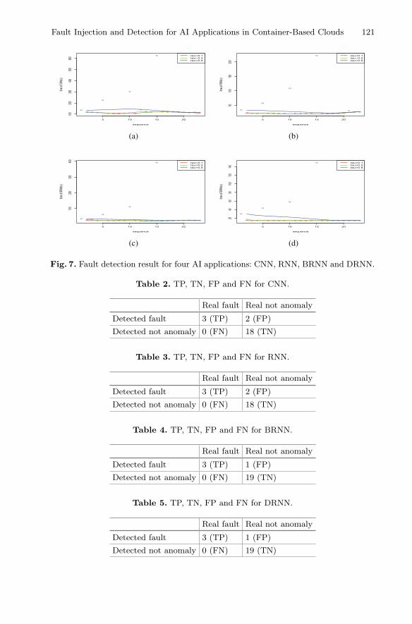
Fault Injection and Detection for AI Applications in Container-Based Clouds 121
Fig. 7. Fault detection result for four AI applications: CNN, RNN, BRNN and DRNN.
Table 2. TP, TN, FP and FN for CNN.
Real fault Real not anomaly
Detected fault 3 (TP) 2 (FP)
Detected not anomaly 0 (FN) 18 (TN)
Table 3. TP, TN, FP and FN for RNN.
Real fault Real not anomaly
Detected fault 3 (TP) 2 (FP)
Detected not anomaly 0 (FN) 18 (TN)
Table 4. TP, TN, FP and FN for BRNN.
Real fault Real not anomaly
Detected fault 3 (TP) 1 (FP)
Detected not anomaly 0 (FN) 19 (TN)
Table 5. TP, TN, FP and FN for DRNN.
Real fault Real not anomaly
Detected fault 3 (TP) 1 (FP)
Detected not anomaly 0 (FN) 19 (TN)

122 K. Ye et al.
Table 6. The Precision, Recall and Accuracy of the detection models for different AIapplications.
Precision Recall Accuracy
CNN application 60% 100% 91.30%
RNN application 60% 100% 91.30%
BRNN application 75% 100% 95.65%
DRNN application 75% 100% 95.65%
based on which, we calculate the Precision, Recall and Accuracy of the detectionmodels in Table 6.
From the above experimental results, it can be seen that the fault detectionmethod based on the quantile regression can effectively detect the potentialfaults. For CNN and RNN fault detection model, the Precision is 60%, Recall is100%, and Accuracy is 91.30%. For BRNN and DRNN fault detection model, thePrecision is 75%, Recall is 100%, and Accuracy is 95.65%. We find the Precisionis relatively low, it is because the number of fault points in the experiment isvery small (3 points) which affects the detection Precision. But if we look at theAccuracy, it is nearly 100% because the number of sampling data is relativelylarge (23 points). We plan to increase the testing scale in the next step of ourwork.
4.3 Detection Models for DDoS Attack
DDOS fault injection detection model needs two sets of data, namely, the receivetraffic and send traffic of the Apache web server. In the experiment, we uses dstattool to collect traffic information. Traffic data is a typical time series type of data,making it ideal for processing using time series models. In the experiment, thequantile regression method is used to process the traffic data in the time series.We totally calculate three groups of fitting values, named fit1, fit2 and fit3, thetau value in each set is set as 0.1, 0.5 and 0.8 respectively. The tau value of0.1 indicates the lower boundary of the receive or send traffic, tau value of 0.5indicates the average value of the receive or send traffic, and the tau value of 0.8indicates the upper boundary of the receive or send traffic. Based on the trainedmodel, we can detect potential DDoS attacks.
Figure 8(a) and (b) shows detection result for both receive and send trafficof Apache Tomcat server under DDoS attacks. In the figure, we inject DDoSattack at point 10, 20, 30, 40, 50, 60, 70, 80, and 90. All the traffic point insidethis range is determined as the normal traffic, while the traffic points outside therange means potential DDOS attack. From the figure, we find the traffic pointswith attacks are obviously outside the confidential interval of the fitting model,which means the fitting model fits the normal traffic data well and can be usedto accurately detect potential DDOS attacks.

Fault Injection and Detection for AI Applications in Container-Based Clouds 123
Fig. 8. Fault detection result for DDoS attacks.
Table 7. TP, TN, FP and FN for the recv traffic.
Real fault Real not anomaly
Detected fault 9 (TP) 0 (FP)
Detected not anomaly 0 (FN) 85 (TN)
Table 8. TP, TN, FP and FN for the send traffic.
Real fault Real not anomaly
Detected fault 9 (TP) 1 (FP)
Detected not anomaly 0 (FN) 84 (TN)
Table 9. The Precision, Recall and Accuracy of the detection model for DDoS recvtraffic and send traffic.
Precision Recall Accuracy
Receive traffic 100% 100% 100%
Send application 90% 100% 98.94%
Table 9 shows precision, recall and accuracy results of the detection modelfor DDoS recv traffic and send traffic, which is based on the results of TP, TN,FP and FN as shown in Tables 7 and 8. For the receive traffic detection model,the Precision is 100%, Recall is 100% and Accuracy is also 100%. For the sendtraffic detection model, the Precision is 90%, Recall is 100% and Accuracy is98.94%, indicating our test models perform very well.
5 Related Work
Recently, there is an increasing interest in the performance and reliability issuesof containers.
Performance. Felter et al. [3] explored the performance of traditional vir-tual machine (VM) deployments, and compared them with the use of Linux

124 K. Ye et al.
containers. They used KVM as a representative hypervisor and Docker as acontainer manager. The results showed that containers result in equal or betterperformance than VMs in most cases. Both VMs and containers require tun-ing to support I/O intensive applications. Ruan et al. [21] conducted a series ofexperiments to measure performance differences between application containersand system containers and find system containers are more suitable to sustainI/O-bound workload than application containers. Ye and Ji [13] proposed a per-formance model to predict the application performance running in containers.Higgins et al. [12] evaluated the suitability of Docker containers as a runtimefor high performance parallel execution. Their findings suggest that containerscan be used to tailor the run time environment for an MPI application withoutcompromising performance. Yu et al. [14] designed a flexible container-basedtuning system (FlexTuner) allowing users to create a farm of lightweight virtualmachines (containers) on host machines. They mainly focus on the impact ofnetwork topology and routing algorithm on the communication performance ofbig data applications. Harter et al. [11] proposed Slacker, a new Docker storagedriver optimized for fast container startup. Docker workers quickly provisioncontainer storage using backend clones and minimize startup latency by lazilyfetching container data.
Reliability. Duffield et al. [22] proposed a rule-based anomaly detection on theIP network which correlates the packet and flow level information. Cherkasovaet al. [23] presented an integrated framework of using regression based transac-tion models and application performance signatures to detect anomalous appli-cation behavior. Sharma et al. [24] used the Auto-Regressive models and a time-invariant relationships based approach to detect the fault. Pannu et al. [25] pre-sented an adaptive anomaly detection framework that can self adapt by learningfrom observed anomalies at runtime. Tan et al. presented two anomaly predictionsystems PREPARE [26] and ALERT [27] that integrate online anomaly predic-tion, learning-based cause inference, and predictive prevention actuation to min-imize the performance anomaly penalty without human intervention. They alsoinvestigated the anomalous behavior of three datasets [28]. Bronevetsky et al. [29]designed a novel technique that combine classification algorithms with informa-tion on the abnormality of application behavior to improve detection. Gu et al.[30] developed an attack detection system LEAPS based on supervised statisticallearning to classify benign and malicious system events. Besides, Fu and Xu [31]implemented a failure prediction framework PREdictor that explores correla-tions among failures and forecasts the time-between-failure of future instances.Nguyen et al. [32] presented a black-box online fault localization system calledFChain that can pinpoint faulty components immediately after a performanceanomaly is detected. Most recently, Arnautov et al. [33] described SCONE, asecure container mechanism for Docker that uses the SGX trusted executionsupport of Intel CPUs to protect container processes from outside attacks.
In comparison, we study fault behaviors and interferences of artificial intelli-gence applications on Docker containers. We also propose fault detection mod-els based on quantile regression method to accurately detection the faults incontainers.

Fault Injection and Detection for AI Applications in Container-Based Clouds 125
6 Conclusion
In this paper, we studied the reliability issue of container-based cloud. We firstproposed a fault injection framework for container-based cloud systems. We builta docker container environment installed with TensorFlow deep learning frame-work, and developed four typical attack programs, i.e., CPU attack, Memoryattack, Disk attack and DDOS attack. Then, we injected the attack programsto the containers running typical artificial intelligence applications (CNN, RNN,BRNN and DRNN), to observe the fault behavior and interference phenomenon.After that, we designed different fault detection models based on quantile regres-sion method to detect potential faults in containers. Experimental results showthat the proposed fault detection models can effectively detect the injected faultswith more than 60% Precision, more than 90% Recall and nearly 100% Accuracy.Note that, in this paper we verified that quantile regression based fault detectionmodel can efficiently detect potential faults, but the experimental scale is stillvery small. In the future, we plan to expand the experimental scale and continueto test our approach in more complex environments.
Acknowledgments. This work is supported by the National Basic Research Programof China (Grant No. 2015CB352400), National Natural Science Foundation of China(Grant No. 61702492, U1401258), and Shenzhen Basic Research Program (Grant No.JCYJ20170818153016513, JCYJ20170307164747920).
References
1. Verma, A., Pedrosa, L., Korupolu, M., Oppenheimer, D., Tune, E., Wilkes, J.:Large-scale cluster management at Google with Borg. In: Proceedings of the TenthEuropean Conference on Computer Systems, p. 18. ACM (2015)
2. Lu, C., Ye, K., Xu, G., Xu, C.-Z., Bai, T.: Imbalance in the cloud: an analysis onAlibaba cluster trace. In: 2017 IEEE International Conference on Big Data (BigData), pp. 2884–2892. IEEE (2017)
3. Felter, W., Ferreira, A., Rajamony, R., Rubio, J.: An updated performance com-parison of virtual machines and Linux containers. In: 2015 IEEE InternationalSymposium on Performance Analysis of Systems and Software (ISPASS), pp. 171–172. IEEE (2015)
4. Linux Containers (2017). https://linuxcontainers.org/5. Docker (2017). https://www.docker.com/6. Rkt (2017). https://github.com/rkt/rkt7. OpenVZ (2017). https://openvz.org/8. Amazon EC2 Container Service (2017). https://aws.amazon.com/docker/9. Containers on Google Compute Engine (2017). https://cloud.google.com/
compute/docs/containers/10. Abadi, M., Barham, P., Chen, J., Chen, Z., Davis, A., Dean, J., Devin, M., Ghe-
mawat, S., Irving, G., Isard, M., et al.: TensorFlow: a system for large-scale machinelearning. In: OSDI, vol. 16, pp. 265–283 (2016)
11. Harter, T., Salmon, B., Liu, R., Arpaci-Dusseau, A.C., Arpaci-Dusseau, R.H.:Slacker: fast distribution with lazy Docker containers. In: FAST, pp. 181–195 (2016)
126 K. Ye et al.
12. Higgins, J., Holmes, V., Venters, C.: Orchestrating Docker containers in the HPCenvironment. In: Kunkel, J.M., Ludwig, T. (eds.) ISC High Performance 2015.LNCS, vol. 9137, pp. 506–513. Springer, Cham (2015). https://doi.org/10.1007/978-3-319-20119-1 36
13. Ye, K., Ji, Y.: Performance tuning and modeling for big data applications in Dockercontainers. In: 2017 12th IEEE International Conference on Networking, Architec-ture, and Storage (NAS 2017). IEEE (2017)
14. Yu, Y., Zou, H., Tang, W., Liu, L., Teng, F.: Flex tuner: a flexible container-basedtuning system for cloud applications. In: 2015 IEEE International Conference onCloud Engineering (IC2E), pp. 145–154. IEEE (2015)
15. Summary of the Amazon s3 Service Disruption in the Northern Virginia (us-east-1)Region (2017). https://aws.amazon.com/message/41926/
16. Veeraraghavan, K., et al.: Kraken: leveraging live traffic tests to identify and resolveresource utilization bottlenecks in large scale web services. In: OSDI (2016)
17. Gunawi, H.S., et al.: Why does the cloud stop computing? Lessons from hundredsof service outages. In: SoCC (2016)
18. Tor’s Hammer: A Slow Post DOS Testing Tool (2017). https://sourceforge.net/projects/torshammer/
19. Dstat: Versatile Resource Statistics Tool (2017). https://github.com/dagwieers/dstat
20. De Oliveira, A.B., Fischmeister, S., Diwan, A., Hauswirth, M., Sweeney, P.F.: Whyyou should care about quantile regression. In: Proceedings of the Eighteenth Inter-national Conference on Architectural Support for Programming Languages andOperating Systems (ASPLOS), pp. 207–218. ACM (2013)
21. Ruan, B., Huang, H., Wu, S., Jin, H.: A performance study of containers in cloudenvironment. In: Wang, G., Han, Y., Martınez Perez, G. (eds.) APSCC 2016.LNCS, vol. 10065, pp. 343–356. Springer, Cham (2016). https://doi.org/10.1007/978-3-319-49178-3 27
22. Duffield, N., Haffner, P., Krishnamurthy, B., Ringberg, H.: Rule-based anomalydetection on IP flows. In: IEEE International Conference on Computer Communi-cations (INFOCOM), pp. 424–432. IEEE (2009)
23. Cherkasova, L., Ozonat, K., Mi, N., Symons, J., Smirni, E.: Anomaly? Applicationchange? Or workload change? Towards automated detection of application perfor-mance anomaly and change. In: 2008 IEEE International Conference on Depend-able Systems and Networks (DSN), pp. 452–461. IEEE (2008)
24. Sharma, A.B., Chen, H., Ding, M., Yoshihira, K., Jiang, G.: Fault detection andlocalization in distributed systems using invariant relationships. In: 2013 43rdAnnual IEEE/IFIP International Conference on Dependable Systems and Net-works (DSN), pp. 1–8. IEEE (2013)
25. Pannu, H.S., Liu, J., Fu, S.: Aad: adaptive anomaly detection system for cloudcomputing infrastructures. In: 2012 IEEE 31st Symposium on Reliable DistributedSystems (SRDS), pp. 396–397. IEEE (2012)
26. Tan, Y., Nguyen, H., Shen, Z., Gu, X., Venkatramani, C., Rajan, D.: Prepare:predictive performance anomaly prevention for virtualized cloud systems. In: 2012IEEE 32nd International Conference on Distributed Computing Systems (ICDCS),pp. 285–294. IEEE (2012)
27. Tan, Y., Gu, X., Wang, H.: Adaptive system anomaly prediction for large-scalehosting infrastructures. In: Proceedings of the 29th ACM SIGACT-SIGOPS Sym-posium on Principles of Distributed Computing (PODC), pp. 173–182. ACM(2010)

Fault Injection and Detection for AI Applications in Container-Based Clouds 127
28. Tan, Y., Gu, X.: On predictability of system anomalies in real world. In: 2010IEEE International Symposium on Modeling, Analysis & Simulation of Computerand Telecommunication Systems (MASCOTS), pp. 133–140. IEEE (2010)
29. Bronevetsky, G., Laguna, I., De Supinski, B.R., Bagchi, S.: Automatic faultcharacterization via abnormality-enhanced classification. In: 2012 42nd AnnualIEEE/IFIP International Conference on Dependable Systems and Networks(DSN), pp. 1–12. IEEE (2012)
30. Gu, Z., Pei, K., Wang, Q., Si, L., Zhang, X., Xu, D.: Leaps: detecting camouflagedattacks with statistical learning guided by program analysis. pp. 57–68 (2015)
31. Fu, S., Xu, C.-Z.: Exploring event correlation for failure prediction in coalitions ofclusters. In: Proceedings of the 2007 ACM/IEEE Conference on Supercomputing(SC), pp. 1–12. IEEE (2007)
32. Nguyen, H., Shen, Z., Tan, Y., Gu, X.: Fchain: toward black-box online faultlocalization for cloud systems. In: 2013 IEEE 33rd International Conference onDistributed Computing Systems (ICDCS), pp. 21–30. IEEE (2013)
33. Arnautov, S., Trach, B., Gregor, F., Knauth, T., Martin, A., Priebe, C., Lind,J., Muthukumaran, D., OKeeffe, D., Stillwell, M.L., et al.: Scone: Secure Linuxcontainers with Intel SGX. In: 12th USENIX Symposium on Operating SystemsDesign and Implementation (OSDI) (2016)

Container-VM-PM Architecture: A NovelArchitecture for Docker Container Placement
Rong Zhang1,2, A-min Zhong1,2, Bo Dong1, Feng Tian1,2(&),and Rui Li1
1 Shaanxi Province Key Laboratory of Satellite and Terrestrial Network Tech.R&D, Xi’an Jiaotong University, Xi’an 710049, China
[email protected] School of Electronic and Information Engineering, Xi’an Jiaotong University,
Xi’an 710049, People’s Republic of China
Abstract. Docker is a mature containerization technique used to performoperating system level virtualization. One open issue in the cloud environmentis how to properly choose a virtual machine (VM) to initialize its instance, i.e.,container, which is similar to the conventional problem of VM placementtowards physical machines (PMs). Current studies mainly focus on containerplacement and VM placement independently, but rarely take into considerationof the two placements’ systematic collaboration. However, we view it as a mainreason for scattered distribution of containers in a data center, which finallyresults in worse physical resource utilization. In this paper, we propose a defi-nition named “Container-VM-PM” architecture and propose a novel containerplacement strategy by simultaneously taking into account the three involvedentities. Furthermore, we model a fitness function for the selection of VM andPM. Simulation experiments show that our method is superior to the existingstrategy with regarding to the physical resource utilization.
Keywords: Docker container � Virtual machine � Resource fragmentThree-tier architecture
1 Introduction
Currently, studies in cloud computing mainly focus on the placement of container toVirtual Machine (VM) and the placement of VM to Physical Machine (PM) [1–3],which we denote as “Container-VM” architecture and “VM-PM” architecturerespectively, shown in Fig. 1(a) and (b). They only consider the resource relationbetween two objects, so we call these architectures as two-tier architecture. Techni-cally, when a new Docker container is created, the Swarm master will choose a node tohost it, which has the highest ranking under a given strategy [4, 5]. Provided that thenode is a VM, the decision making mechanism only concerns the resource relationshipbetween the Docker container and VM. Moreover, when a new VM needs to becreated, the OpenStack nova filter scheduler selects correspond PMs according to agiven weighting functions [6, 7]. The new VM placement decision making thus onlyconcerns the resource relationship between the new VM and PMs, which ignores the
© Springer International Publishing AG, part of Springer Nature 2018M. Luo and L.-J. Zhang (Eds.): CLOUD 2018, LNCS 10967, pp. 128–140, 2018.https://doi.org/10.1007/978-3-319-94295-7_9
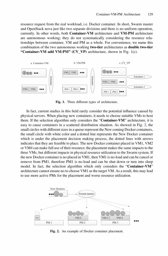
resource request from the real workload, i.e. Docker container. In short, Swarm masterand OpenStack nova just like two separate divisions and there is no uniform operation,currently. In other words, both Container-VM architecture and VM-PM architectureare autonomous working; they do not systematically considering the resource rela-tionships between container, VM and PM as a whole. For convenience, we name thiscombination of the two autonomous working two-tier architectures as double two-tier“Container-VM add VM-PM” (CV_VP) architecture, shown in Fig. 1(c).
In fact, current studies in this field rarely consider the potential influence caused byphysical servers. When placing new containers, it needs to choose suitable VMs to hostthem. If the selection algorithm only considers the “Container-VM” architecture, it iseasy to cause containers in a scattered distribution situation. As showed in Fig. 2, thesmall circles with different sizes in a queue represent the New coming Docker containers,the small circle with white color and a dotted line represents the New Docker containerwhich is under the placement decision making process, the dotted lines with arrowsindicates that they are feasible to place. The new Docker container placed in VM1, VM2or VM4 can make full use of their resource; the placement makes the same impacts to thethree VMs, but different impacts in physical resource utilization to the Swarm system. Ifthe newDocker container is no placed in VM1, then VM1 is no-load and can be cancel orremove from PM1, therefore PM1 is no-load and can be shut down or turn into sleepmodel. In fact, the selection algorithm which only considers the “Container-VM”architecture cannot ensure no to choose VM1 as the target VM. As a result, this may leadto use more active PMs for the placement and worse resource utilization.
c. CV_VPb. VM-PMa. Container-VM
1 2 3
VM1 VM2
PM 1 PM 2
Scheduler 1Scheduler
1 2 3
VM1 VM2
Scheduler
PM 1 PM 2
VM1 VM2
Scheduler 2
Fig. 1. Three different types of architecture.
PM 1
VM 1
PM 2
VM 2
PM 3
VM 3 VM 4
New Dockers
Swarm master
Fig. 2. An example of Docker container placement.
Container-VM-PM Architecture 129

To solve this problem, the resource relationships between container, VM and PMshould be systematically considered as a whole, we denote their collaborative operatingarchitecture as a three-tier “Container-VM-PM” (CVP) architecture, shown in Fig. 3.
However, current studies rarely consider the three as a whole, there is very littleliterature about this concept. Tchana et al. [8] proposed the implementation of thesoftware consolidation based on the assumption that Docker is used for software iso-lation and the same VM be shared between several soft applications. The authors wantto extend analysis of best coordinate software consolidation on VMs with VM con-solidation on physical machines in their future work. Their idea involves CVP archi-tecture which coincides with ours, although it is their future work. Still, it inspires us. Inthis paper, we try to solve the new Docker container placement problem under the CVParchitecture, taking the minimum active PMs as the first goal and maximum resourceutilization as the second goal.
Due to the collaborative operations, the placement algorithm towards new Dockercontainers is more complicated under the CVP architecture, which raises threechallenges:
– Which PM should be chosen?– Which VM should be chosen?– How to coordinate the placement of Docker containers to VMs, considering the
placement of VMs to PMs simultaneously.
We propose a container placement strategy under CVP architecture and make afitness model to select the optimal VMs and PMs. We also leverage the Best-fitalgorithm to search the optimal mapping. Finally, we derive the mapping relationshipbetween container, VM and PM. To the best of our knowledge, this work is the firstthat systematically considers the resource relationships between container, VM and PMand coordinates the placement of Docker containers to VMs with the placement ofVMs to PMs simultaneously.
Our main contributions are as follows:
(1) We focus on the Docker container placement problem in order to improve thephysical resource utilization.
(2) We systematically consider the resource relationships between container, VM andPM as a whole and extend the study from two-tier architecture to a three-tier“Container-VM-PM” architecture.
1 2 3
VM1 VM2
PM 1 PM 2
Scheduler
Fig. 3. The CVP architecture.
130 R. Zhang et al.

(3) We propose a Docker container placement strategy under the three-tier“Container-VM-PM” architecture and establish a VM and PM selection model.
The rest of this paper is organized as follows. Related works and some importantdefinitions are reviewed in Sect. 2. In Sect. 3, we describe the key problem and ourproposed method. Furthermore, we propose an evaluation formula for the placementperformance comparison. Experiments and results are showed in Sect. 4. Conclude andfuture work in Sect. 5.
2 Background
In this section, we introduce the concept of Docker container and Virtual Machine.More concretely, we first compare the pros and cons of the two techniques and reviewtheir related research in the literature. Then, we introduce the definitions of resourceutilization and resource fragmentation. Last, we introduce the Best-fit algorithm thatwill adopt.
2.1 Docker Container and Virtual Machine
Docker [9], an open sourced project, provides a lightweight virtualization mechanismat system level and automates a faster deployment of Linux applications by extending acommon container format called Linux Containers (LXC) [10]. It can be deployed onVMs or “bare metal” physical servers. In most cases, a container can be created anddestroyed in almost real-time and introduces negligible performance overhead towardsCPU and memory [11]. It thus is suitable to quickly build and restructure applicationservices. Compared with VMs, containers have advantages of fast deployment andmigration, but they also suffer from weak isolation and security. Therefore, many cloudservice providers take a compromise solution by combining the two techniques, i.e.,they place containers in VMs. As cloud business services thrive in recent years, therequirement for efficiently placing containers while maximizing resource utilization hasattracted a wide range of attention [12].
VMs are widely used in cloud computing. Various kinds of service models areoffered by Cloud computing service, there are three kinds of service models that havebeen popular accepted: Infrastructure as a Service (IaaS), Platform as a Service (PaaS)and Software as a Service (SaaS) [13]. Many enterprises use their cloud platforms tomake VMs available to the end user and even run services inside VMs. One ofextensively used open source cloud platform is OpenStack. Nova is an importantcompute component of OpenStack. OpenStack Nova is responsible for provisioningand management of VMs [14]. The detail information about its scheduling strategy isreferring to [15, 16].
Many Platform providers built their PaaS and SaaS on IaaS, and run all theworkload inside VMs. Swarm plays an important role in PaaS and SaaS, which is usedto manage the Docker cluster. Scheduling strategy on Swarm can be introduced from[17, 18] in detail.
Container-VM-PM Architecture 131

2.2 Resource Utilization
Both the Container placement problem under Container-VM architecture and the VMplacement problem under VM-PM architecture can be described as a bin packingproblem. For this reason, we can transform the Container-VM architecture as Fig. 4(a),and the VM-PM architecture could be showed as Fig. 4(b).
As shown in the Fig. 4(a), the real workloads are Container 1 and Container 2.Although the VM requests for cvm CPU and mvm Memory resources, but the effectiveresources utilization are (cc1 + cc2) CPU and (mc1 + mc2) Memory. As shown in theFig. 4(b), it only concerned about the resources of VM and ignores the container layer.The physical resource utilization is calculated by summing resources occupied by theVMs hosted by the PM.
The CVP architecture can be transformed as Fig. 4(c). It systematically considersthe resource relationships between container, VM and PM as a whole. Because of thereal workloads are containers, the effective resources utilization are calculated by theresources of containers. As a result, the physical resource utilization is calculated bysumming resources occupied by the containers run in the PM. As the resource infor-mation of the three layers is clear, it can help to place new Docker containers moreeffectively.
2.3 Resource Fragmentation
Different containers need to occupy different dimensions of resources. A node can hosta container when it meets the container’s resources requirement in every dimension.After new container placement, the unused resources are called Resource Fragmenta-tion [17, 19].
If the resource fragmentations are too small, it may unable to accept more newobjects’ placement. So, the size of resource fragmentations is the bigger the better inthe case of using same amount of active PMs.
VM
Container 1
Container 2
CPU
Memmvm
cvmcc1 cc1+cc20
mc1
mc1+mc2
PMcvm1
VM1
VM2
CPU
Mem
cvm1+cvm2
mvm1
mvm1+mvm2
100%
100%0
a. Container-VM
b. VM-PM
PMcvm1
VM1
VM2
CPU
Mem
cvm1+cvm2
mvm1
mvm1+mvm2
100%
100%0
Container 1
Container 2
Container 3
c. Container-VM-PM(CVP)
Fig. 4. Three different types of architecture in two-dimension.
132 R. Zhang et al.

2.4 Best-Fit Algorithm
Best-fit algorithm is a fast allocation algorithm and it is commonly used in solving thebin packing problem. For an upon arrival item, Best-fit algorithm chooses a fullest bin,in which it fits from a list of current bins to host the item; in case this process fails, anew bin for the item will be opened [20]. As a result, when Best-fit algorithm is used inthe placement of Docker container to VM, we treat Docker containers as the items andtreat VMs as bins. Similarly, when Best-fit algorithm is used in the placement of VM toPM, we treat VMs as the items and treat PMs as bins. Furthermore, resource frag-mentation is used to evaluate the bin in order to judge if it is the fullest one or not.
3 Methods and Problem Formulation
The key in the new Docker container placement problem is how to choose the suitableVM and PM. In this section, we will give a new Docker container placement strategyreferring to the placement strategies in [8, 9]. As it’s different in the view point ofresource relations between CV_VP and CVP architecture, the VM and PM selectionstrategies are different too. We thus model the VM and PM selection fitness functionfor CV_VP and CVP architecture respectively. Furthermore, we propose an evaluationformula for the placement performance comparison.
To simplicity and clarity, we make the following assumptions:
(1) Each Docker container should be hosted by one VM, and several Docker con-tainers can be placed in a same VM.
(2) All PMs have the same configuration.(3) Only focus on two-dimension resources, they are CPU and Memory.
Considering taking the minimum active PMs as the first goal and maximumresource utilization as the second goal, we propose a placement strategy for the newDocker container and the VM and PM selection strategy for the two architectures,respectively. The notations used in this paper are described in Table 1.
3.1 The Placement Strategy Under CV_VP Architecture
When dealing with a new Docker container, the Docker container should be placed inthe current existing VMs preferentially. There are two situations that need to beconsidered.
(1) If there does not exists any VM that can host the new Docker container, thesmallest VM which can host the new Docker container should be selected fromthe VM provision set as the new VM. This new VM is the target VM. Certainlywe need to choose a suitable PM to host the new VM. There are two possiblescenarios.One scenario: Suppose that there are m active PMs which can host the new VM,where m[ 0. Because of the CV_VP architecture, the PM selection is onlydepending on the new VM’s resource requests. For each PM in the m active PMsSet, we take the sum of its CPU and memory resources utilization after the new
Container-VM-PM Architecture 133

VM placement as its fitness. So, the fitness function PAfitðjÞ for the j active PMcan be defined as:
PAfitðjÞ ¼ cpuVusedj þ cpuvmnewcpupmj
� aþ memVusedj þmemvm
new
mempmj
� b; ð1Þ
where, j ¼ 1; � � � ;m, a and b are two constants, represent the two parts’ weights ofthe formula. At last, the PM which has the max fitness will be chosen to host thenew VM. This PM will be the target PM.The other scenario: Suppose that there does not exist any active PM that can hostthe new VM, then an idle PM should be start. The new active PM will be thetarget PM.
(2) If there exists n VMs that can host the new Docker, where n[ 0. Because of theCV_VP architecture, the VM selection is only depending on the new Docker’sresource requests. For each VM in the n exist VMs Set, we take the sum of itsCPU and memory resources utilization after the new Docker container placementas its fitness. So, the fitness function VAfitðiÞ for the VM i can be defined as:
VAfitðiÞ ¼ cpuDusedi þ cpuDockernew
cpuvmi� aþ memDused
i þmemDockernew
memvmi
� b; ð2Þ
where, i ¼ 1; � � � ; n. At last, the VM which has the max value of VAfit will bechosen to host the new Docker container. This VM will be the target VM, and thePM which hosts this VM will be the target PM.
Table 1. Notations.
Symbol Description
cpuVusedj The sum of the VMs’ CPU resource in the jth active PM
memVusedj The sum of the VMs’ Memory resource in the jth active PM
cpupmj The total CPU resource of the jth active PM
mempmj The total Memory resource of the jth active PM
cpuDusedi The sum of the Docker containers’ CPU resource in the ith VM
memDusedi The sum of the Docker containers’ Memory resource in the ith VM
cpuvmi The total CPU resource of the ith VMmemvm
i The total Memory resource of the ith VM
cpuDockernew The CPU resource that the new Docker container request for
memDockernew The Memory resource that the new Docker container request for
cpuDusedj The sum of the Docker containers’ CPU resource in the jth active PM
memDusedj The sum of the Docker containers’ Memory resource in the jth active PM
NactivePM The number of active PM
cpuremainj The remain CPU resources of the jth active PM
memremainj The remain Memory resources of the jth active PM
134 R. Zhang et al.

3.2 The Placement Strategy Under CVP Architecture
There are two situations that need to be considered too, but some parts of the calcu-lation are different from CV_VP architecture.
(1) If there does not exists any VM that can host the new Docker, the smallest VMwhich can host the new Docker should be selected from the VM provision set asthe new VM. This new VM is the target VM. Certainly we need to choose asuitable PM to host the new VM. There are two possible scenarios.One scenario: Suppose there are m active PMs which can host the new VM,where m[ 0. We define the fitness function PBfitðjÞ for the j active PM as:
PBfitðjÞ ¼ cpuDusedj þ cpuDockernew
cpupmj� aþ memDused
j þmemDockernew
mempmj
� b; ð3Þ
where, j ¼ 1; � � � ;m. At last, the PM which has the max value of PBfit will bechosen to host the new Docker container. This PM will be the target PM.The other scenario: Suppose there does not exist any active PM that can host thenew VM, then an idle PM should be start. The new active PM will be the targetPM.
(2) If there exists n VMs that can host the new Docker, where n[ 0. The VMselection is not only depending on the new Docker’s resource requests but alsodepending on the real resource utilizations because of the CVP architecture. Theplacement of a new container should better improve the resource utilization of thetarget PM and the target VM. So, the fitness function VBfitðiÞ for the VM i can bedefined as:
VBfitðiÞ ¼ cpuusedi þ cpuDockernew
cpuvmi� aþ memused
i þmemDockernew
memvmi
� bþPBfitðkÞ � dik;
ð4Þ
i ¼ 1; � � � ; n; dik ¼ 1; if PM k hosts VM i0; the other
�;
where, the first part and the second part of the fitness function are used torepresent the new Docker container placement impact on VM resourcesutilization, the third part represent the impact on PM resources utilization. Atlast, the VM which has the max value of VBfit will be chosen to host the newDocker container. This VM will be the target VM, and the PM which hosts thisVM will be the target PM.
3.3 Evaluation Model
Because of the requested resource by a VM is not fully utilized in most situations, it ismore accurate to calculate the real resource utilization by the real workloads’ resource
Container-VM-PM Architecture 135

requests. The real workloads are Docker containers, so the evaluation formula Escorecan be given as follows:
Escore ¼ aE � NactivePM þ bE �
Xj
cpuremainj � memremainj
� �; ð5Þ
cpuremainj ¼ cpuPMj � cpuDusedj ; ð6Þ
memremainj ¼ memPM
j � memDusedj ; ð7Þ
where, aE and bE are two constants, represent the two parts’ weights of Escore.aE [ 0[ bE and aE [ [ bEj j. The first part of Escore is to make sure that taking theleast active PMs as the first goal, and the second part is used to distinguish the size ofresource fragmentations when using the same amount of active PMs. The evaluationscore is the small the better.
4 Experiments and Results
In this section, a method is introduced to generate Docker container Synthetic Instancesand 16 types of VM instance from Amazon EC2 are constituted as our VM provisionset. The experiment simulates to deal with 9 batches of new Docker containers’placement consecutively. Finally we evaluate the physical resource utilization betweenCV_VP and CVP architecture after the new Docker container placement.
4.1 Docker Container Synthetic Dataset
A method is introduced to generate Docker container Synthetic Instances from [21, 22]into this paper. The method is showed in Algorithm 1.
where, randðaÞ will return a random number in the range 0; a½ Þ; ucpu and umem arerepresent the reference CPU and Memory utilization respectively. The probabilityP can be used to control the correlation of CPU and Memory utilizations.
136 R. Zhang et al.

4.2 VM Dataset
As outlined in Table 2, 16 types of VM instance from Amazon EC2 are imported asour VM provision set.
4.3 Parameter Setting
In this paper, our parameters are outlined in Table 3.
4.4 Experimental Comparison
After dealing with 9 batches of new Docker container placement consecutively, weevaluate the physical resource utilization between CV_VP and CVP architecture. Theresults are showed as Table 4 and Fig. 5.
As shown in Table 4, after the placement of first batch of containers, the totalnumber of Docker container is 787. It uses 292 active PMs and its evaluation score is28727.866 under CV_VP architecture, however it uses only 244 active PMs that is
Table 2. VM instance types from Amazon EC2.
VM instance type vCPU Memory (GiB)
t2.micro 1 1t2.small 1 2t2.medium 2 4t2.large 2 8m3.medium 1 3.75m3.large 2 7.5c4.large 4 7.5r4.xlarge 4 30.5r4.2xlarge 8 61r4.4xlarge 16 122r4.8xlarge 32 244m4.4xlarge 16 64m4.10xlarge 40 160g2.8xlarge 32 60g3.4xlarge 16 122d2.8xlarge 36 244
Table 3. The related parameter values.
Container-VM-PM Architecture 137

0.8536 times of CV_VP and its evaluation score is 24283.9 under CVP architecturethat is 0.8453 times of CV_VP. After the placement of nine batches of Docker con-tainers, the total number of Docker container is 225627. It uses 80223 active PMs andits evaluation score is 7906899 under CV_VP architecture, however it uses only 66103active PMs that is 0.8240 times of CV_VP and its evaluation score is 6593462.821under CVP architecture that is 0.8399 times of CV_VP. The experimental results showthat the placement under CVP architecture uses less active PMs and get a betterevaluation score than the placement under CV_VP architecture. New Docker containerplacement is more effective in physical resource utilization under CVP architecture.
Table 4. Comparison of the placement under CV_VP and CVP architecture.
No. Dockercontainers
CV_VP CVP The ratio of CVP toCV_VP
Active Pms Escore Active Pms Escore Active Pms Escore
1 787 292 28727.866 244 24283.900 0.8356 0.84532 1019 377 37094.847 311 30978.971 0.8249 0.83513 2297 827 81556.531 707 70406.169 0.8549 0.86334 5014 1819 179197.533 1493 148878.131 0.8208 0.83085 10129 3613 356197.028 3011 300239.999 0.8334 0.84296 12569 4485 356197.028 3704 369394.082 0.8259 0.83587 124984 44516 4386860.736 36563 3647070.301 0.8213 0.83148 149601 53116 5235826.403 43893 4377877.318 0.8264 0.83619 225627 80223 7906899.000 66103 6593462.821 0.8240 0.8399
Fig. 5. Escore comparison.
138 R. Zhang et al.

5 Conclusion and Future Work
In this paper, we have extended the study from two-tier architecture to three-tier“Container-VM-PM” (CVP) architecture. We focus on the new Docker containerplacement problem under the CVP architecture, and compare it with the placementunder CV_VP architecture. The results show that the former is more effective than thelatter in physical resource utilization.
The resource utilization can be observed in a global view under CVP architecture,so it can be more conducive to utilize the resource effectively. Based on this advantage,we want to extend our study on Container consolidation and load balance under theCVP architecture in our future work. We also want to test more algorithms in order tofully show their performances under the CVP architecture.
Acknowledgement. This work is supported by National Key Research and DevelopmentProgram of China under Grant No. 2016YFB1000303, Innovative Research Group of theNational Natural Science Foundation of China (61721002), Innovation Research Team ofMinistry of Education (IRT_17R86), the National Natural Science Foundation of China(61502379, 61532015, 61672410, 61472315, 61428206, 61532015 and 61532004), the Projectof China Knowledge Centre for Engineering Science and Technology.
References
1. Affetti, L., Bresciani, G., Guinea, S.: aDock: a cloud infrastructure experimentationenvironment based on open stack and Docker. In: IEEE International Conference on CloudComputing (2015)
2. Kaewkasi, C., Chuenmuneewong, K.: Improvement of container scheduling for Dockerusing Ant Colony Optimization. In: International Conference on Knowledge and SmartTechnology, pp. 254–259. IEEE (2017)
3. Rathor, V.S., Pateriya, R.K., Gupta, R.K.: Survey on load balancing through virtual machinescheduling in cloud computing environment. Int. J. Cloud Comput. Serv. Sci. (IJ-CLOSER)3(1), 37 (2014)
4. Docker Swarm Strategies. https://docs.docker.com/swarm/scheduler/strategy/5. Docker/Awarm. https://github.com/docker/swarm/tree/master/scheduler/strategy6. Filter Scheduler. https://docs.openstack.org/nova/latest/user/filter-scheduler.html7. OpenStack/Nova. https://github.com/openstack/nova/tree/master/nova/scheduler8. Tchana, A., Palma, N.D., Safieddine, I., Hagimont, D., Diot, B., Vuillerme, N.: Software
consolidation as an efficient energy and cost saving solution for a SaaS/PaaS cloud model.In: Träff, J.L., Hunold, S., Versaci, F. (eds.) Euro-Par 2015. LNCS, vol. 9233, pp. 305–316.Springer, Heidelberg (2015). https://doi.org/10.1007/978-3-662-48096-0_24
9. Naik, N.: Applying computational intelligence for enhancing the dependability ofmulti-cloud systems using Docker swarm. In: Computational Intelligence (2017)
10. Bernstein, D.: Containers and cloud: from LXC to Docker to kubernetes. IEEE CloudComput. 1(3), 81–84 (2015)
11. Felter, W., et al.: An updated performance comparison of virtual machines and Linuxcontainers. In: IEEE International Symposium on PERFORMANCE Analysis of Systemsand Software (2015)
Container-VM-PM Architecture 139
12. Mao, Y., et al.: DRAPS: dynamic and resource-aware placement scheme for dockercontainers in a heterogeneous cluster. In: IEEE – International PERFORMANCE Comput-ing and Communications Conference (2017)
13. Bhardwaj, T., Kumar, M., Sharma, S.C.: Megh: a private cloud provisioning various IaaSand SaaS. In: Pant, M., Ray, K., Sharma, T.K., Rawat, S., Bandyopadhyay, A. (eds.) SoftComputing: Theories and Applications. AISC, vol. 584, pp. 485–494. Springer, Singapore(2018). https://doi.org/10.1007/978-981-10-5699-4_45
14. Datt, A., Goel, A., Gupta, S.C.: Analysis of infrastructure monitoring requirements forOpenStack Nova. Procedia Comput. Sci. 54, 127–136 (2015)
15. Hu, B., Yu, H.: Research of scheduling strategy on OpenStack. In: International Conferenceon Cloud Computing and Big Data (2014)
16. Sahasrabudhe, S., Sonawani, S.S.: Improved filter-weight algorithm for utilization-awareresource scheduling in OpenStack. In: International Conference on Information Processing(2016)
17. Tseng, H.W., Wu, R.Y., Chang, T.S.: An effective VM migration scheme for reducingresource fragments in cloud data centers (2014)
18. Lu, S., Ni, M., Zhang, H.: The optimization of scheduling strategy based on the Dockerswarm cluster. Information Technology, pp. 147–155 (2016)
19. Huang, W., Li, X., Qian, Z.: An energy efficient virtual machine placement algorithm withbalanced resource utilization. In: Seventh International Conference on Innovative Mobileand Internet Services in Ubiquitous Computing (2013)
20. Kenyon, C.: Best-fit bin-packing with random order. In: ACM-SIAM Symposium onDiscrete Algorithms (1996)
21. Gao, Y., et al.: A multi-objective ant colony system algorithm for virtual machine placementin cloud computing. J. Comput. Syst. Sci. 79(8), 1230–1242 (2013)
22. Tian, F., et al.: Deadlock-free migration for virtual machine consolidation using ChickenSwarm Optimization algorithm. J. Intell. Fuzzy Syst. 32, 1389–1400 (2017)
140 R. Zhang et al.

Research Track: Cloud ResourceManagement
Renewable Energy Curtailmentvia Incentivized Inter-datacenter
Workload Migration
Ahmed Abada(B) and Marc St-Hilaire
Department of Systems and Computer Engineering,Carleton University, Ottawa, ON, Canada
{ahmed.abada,marc st hilaire}@carleton.ca
Abstract. Continuous Grid balancing is essential for ensuring the reli-able operation of modern smart grids. Current smart grid systems lackpractical large-scale energy storage capabilities and therefore their sup-ply and demand levels must always be kept equal in order to avoid systeminstability and failure. Grid balancing has become more relevant in recentyears following the increasing desire to integrate more Renewable EnergySources (RESs) into the generation mix of modern grids. RESs produceintermittent energy supply that can’t always be predicted accurately [1]and necessitates that effective balancing mechanisms are put in placeto compensate for their supply variability [2,3]. In this work, we pro-pose a new energy curtailment scheme for balancing excess RESs energyusing data centers as managed loads. Our scheme uses incentivized inter-datacenter workload migration to increase the computational energy con-sumption at a destination datacenter by the amount necessary to bal-ance the grid. Incentivised workload migration is achieved by offeringdiscounted energy prices (in the form of Energy Credits) to large-scalecloud clients in order to influence their workload placement algorithmsto favor datacenters where the energy credits can be used. Implementa-tions of our system using the CPLEX ILP solver as well as the Best FitDecreasing (BFD) heuristic [4] for workload placement on data centersshowed that using energy credits is an effective mechanism to speed-up/control the energy consumption rates at datacenters especially atlow system loads and that they result in increased profits for the cloudclients due to the higher profit margins associated with using the pro-posed credits.
1 Introduction
The lack of large-scale energy storage solutions in modern smart-grids necessi-tates that their energy generation and consumption levels are always kept equalin order to avoid system instability and service interruptions. Since making onlinefine adjustments to the energy levels of the generators supplying the grid canbe costly (because of the different start-up/shut-down delay constraints of eachgenerator and the monetary costs associated with making such adjustments),c© Springer International Publishing AG, part of Springer Nature 2018M. Luo and L.-J. Zhang (Eds.): CLOUD 2018, LNCS 10967, pp. 143–157, 2018.https://doi.org/10.1007/978-3-319-94295-7_10

144 A. Abada and M. St-Hilaire
many Demand-Response (DR) proposals were introduced by the utility compa-nies to exploit the demand-side flexibility of energy consumers for grid balancing.DR programs generally aim to control the consumers demand for electricity byusing monetary incentives such as variable pricing or time-of-use pricing [5–7]. Commercial class energy consumers have been the main focus of many DRproposals because of their higher consumption rates and the higher demandelasticity of some commercial consumers compared to their residential counter-parts. Datacenter plants in particular have received a significant share of DRproposals because of their consistent rapid growth in recent years (as a result ofthe increasing popularity of cloud computing applications) and their ability tocontrol their energy consumption levels by using different energy managementtechniques or adjusting the scheduling of their computational workloads [8–11]
Data centers are known to consume a lot of energy to operate since theytypically comprise several thousands of computing and networking equipmentsin a physically monitored environment [12]. The high energy consumption ofdatacenters has attracted many optimization research efforts [13]. Traditionallythe main focus has been on minimizing their energy consumption cost eitherby sever consolidation [14–16], using DVFS [17] or by proposing different work-load scheduling/migration techniques that take advantage of variable real-timeenergy prices to process more workloads when the prices are low [18,19]. Morerecently, following the growing demand to integrate more green RESs into thegeneration mix of modern smart grids, more attention was given to datacentersas controllable loads that could play a major role in enabling the integration ofmore RESs by compensating for their intermittent supply and help maintain thegrid balance. Such DR related research is mainly concerned with the effectiveintegration of data centers as a “resource” or a “managed load” into the varioussmart grid based DR programs [5,8,20].
Because of their highly intermittent supply, it can be a challenge for the gridto maintain its balance at times of excess RESs energy generation. Hence, theability of the grid to achieve timely and effective renewable energy curtailmenthave been a distinctive hurdle that needed to be addressed more effectively inorder to increase the amount of renewable energy deployment into the generationmix of modern grids [21]. Events of unexpected excess RESs energy generationcan lead to system instability and utility companies opt at times to apply nega-tive energy prices in order to re-balance the grid in a timely manner. However,grid failures can still occur due to such events [22,23].
The curtailment of renewable energy have been studied in the past to ensurebalanced grid operation [3,24]. However, unlike existing curtailment strategiesthat blocks excess RESs energy from entering into the system [25], in this work,we try to leverage the demand side flexibility of datacenters in order to effec-tively balance the excess RESs energy. Hence, our proposal has the advantageof putting the excess RESs energy to use rather than simply discarding it. Wepresent a new energy curtailment approach that uses data centers as managedloads to allow the grid system more “downward flexibility” (i.e. the ability tocope with extra supply or low demand). Our approach is based on offering dis-
Renewable Energy Curtailment 145
counted energy cost (a monetary incentive in the form of Energy Credits) tolarge-scale cloud users to incentivize them to migrate their computational work-loads to datacenters connected to the part of the grid having excess RESs energysupply. The amount of Energy credits offered is made equal to the amount ofenergy that a grid would need to consume in a timely manner in order to staybalanced. We formulate our problem as a linear integer programming problemwith the objective of minimizing the cost of assigning computational workloadson available datacenters. We present our simulation results from implementingour model using the CPLEX ILP solver as well as the Best Fit Decrteasing(BFD) workload assignment heuristic [4] that can be more practical in largescale operations.
The remainder of this paper is organized as follows: in the next sectionwe briefly discuss previous work related to earlier data center based demand-response efforts and discuss the importance of these efforts as an enabler forintegrating more renewable energy sources into the generation mix of modernsmart grids. Section 3 introduces our cloud-broker based grid balancing proposaland presents its system model and optimization formulation. We present theperformance analysis conducted on our system in Sect. 4 and finally concludethe paper in Sect. 5.
2 Related Work
Since data centers represent a significant load for the smart grids that they drawpower from, many research efforts have proposed closer cooperation between thetwo in order to ensure a smooth operation on both sides [11,26]. An example ofsuch tight coupling between the power grid and the data center is in [27] whichtries to save on the datacenter energy cost by deploying backup batteries locallyat the datacenter and charging them at times of low electricity prices then usingthem to power the datacenter when the prices are higher. The significance ofdata centers as energy loads and their ability to increase/decrease their energyconsumption by adjusting their computational workload scheduling represents avaluable opportunity for the smart grid operators to essentially integrate themas managed loads for grid balancing purposes using DR [6,10].
A successful integration between the datacenters and smart grids would allowthe datacenters to be considered as a “resource” by the smart grid operatorwhich in turn can then use it for grid balancing purposes. However, a mainobstacle towards this integration is that modern data centers are increasinglybecoming colocation based [28], where multiple organizations host their comput-ing/networking equipment at a shared physical location in order to save on man-agement and maintenance costs. In such environments, the colocation operatorhas no direct control on the workload scheduling or the energy-saving/server-consolodation techniques applied by the tenants. This makes the involvement ofsuch data centers in modern DR programs more challenging compared to thetraditional case of owner-operated data centers as described in [29]. Collocationoperators suffer from the “split-incentive” phenomenon that hinders their par-ticipation in DR programs. On one hand, they desire to get the monetary gains

146 A. Abada and M. St-Hilaire
associated with participating in DR programs, yet, they have no direct way tocontrol the energy consumption of their tenants.
Effective grid balancing is also necessary for enabling large-scale integrationof RESs into the smart-grid. The integration of such sources into the genera-tion mix of modern smart grids have made significant progress in recent years.However, because of the indeterministic nature of the power generated by suchsources (wind/solar) and the unavailability of large-scale energy storage facilitiesin modern grid systems, their rate of adoption into the generation-mix of moderngrids has been mainly limited by the grid’s ability to stay in balance given thenature of their intermittent supply [9]. Recent research [1] points to the fact thatexcess energy from RESs could often need to be discarded in order to keep thegrid in balance. In some cases negative pricing is applied just to achieve a timelybalancing of the grid and avoid service interruption. Negative/free energy pricingis applied at times of excess RESs supply when it is cheaper to offer the excessenergy for free or at a negative price than to shut down generation facilities andrisk future service interruptions. The rapid increase of datacenter deploymentsin recent years is positioned to play an important role in enabling the integra-tion of more RESs into the smart-grids by acting as a managed load that caneffectively absorb the introduced supply variability of RESs sources.
A main challenge to overcome in this regard is how to effectively influencethe workload scheduling on the datacenter servers in order to comply with theDR requirements. This is not easy to accomplish in current colocation based dat-acenters since they lack coordination between the colocation operator and thetenants in charge of workloads scheduling on the servers. On one hand, the colo-cation operator is interested in complying with DR programs so it can qualify forfinancial incentives, but on the other hand, the colocation tenants are only inter-ested in achieving maximum performance for their workloads since they have nodirect relationship with the grid operator and would not receive any financialgain for adjusting their workload if they comply with the requirements of theDR programs. We suggest in this work that establishing a direct relationshipbetween large scale colocation tenants (such as cloud brokers) and the utilitycompany/grid can lead to a more effective DR implementation in the datacen-ter domain. Previous work in this area has investigated several mechanisms forextending demand response programs to colocation based datacenters [29–31].However with the continuing demand for increased renewable energy integra-tion in modern smart grids, a tighter coupling between the grid and datacenters(including their tenants) is of great value in order to take full advantage of thedatacenters as managed loads.
3 Cloud-Broker Based Grid Balancing
As opposed to existing demand-response approaches that only target data cen-ter operators (that don’t necessarily have direct control on workload schedul-ing in the case of colocations), we propose a new mechanism that would allowextending such programs to the enterprise-type tenants (such as Cloud Brokers

Renewable Energy Curtailment 147
and SaaS/PaaS operators) of colocation data centers. Such tenants typicallyhost their hardware at multiple colocations in different geographical locations toachieve high redundancy and shorter response times. Their workloads accountfor a large share of the total workloads handled by modern colocation data cen-ters. Hence, they can be considered as a resource or a managed load that smartgrids can use to scale up/down the energy consumption in order to meet DRgoals.
Our approach is based on introducing a “Market” entity as a communica-tion medium between the grid/utility company and the cloud-broker/colocation-tenant as shown in Fig. 1. When a grid/utility company needs to balance acertain amount of excess RESs energy, it generates a number of energy creditsequal to the amount of excess RESs energy that needs to be balanced/consumed.Such energy credits are then offered (at a discounted cost) to the cloud bro-kers/collocation tenants to incentivize them to migrate their workloads fromother datacenter locations to a certain datacenter whose energy consumptionneeds to be increased to balance the excess RESs energy. The proposed energycredits are made available to the brokers via the central market entity (“ECMarket”) that handles all the energy credits assignments/transactions betweenthe different utility companies and cloud brokers/colocation tenants. Our sys-tem model shown in Fig. 1 comprises four main entities, cloud brokers/colocationtenants, colocation data centers, utility companies (grid) and the EC market. Weconsider a single cloud broker in our model for simplicity, however, the systemcan be expanded to handle multiple brokers via game theoretic approaches. Eachdata center is assumed to adopt a different pricing model based on its popular-ity and the offered performance guarantees. Cloud brokers continuously receivecomputing workloads (i.e. Requests) of different weights from their clients andthey need to optimally assign/schedule the received workloads on the availabledata centers to maximizes their return.
We assume that each incoming workload (WL) received by a broker has threemain attributes, a Computing weight (WLcpu) that describes how much com-puting resources it requires, a Memory weight (WLmemory) that describes howmuch storage capacity it requires and an Energy Consumption weight (WLkWh)that describes how much energy it is rated to consume per unit time. We fur-ther assume that the cloud broker implements a fixed pricing model whereby itsclients are charged solely based on the computing and storage weights of theirsubmitted workloads at the rates Ccpu
B and CmemoryB respectively. Accordingly,
the broker’s profit P that the broker charges for handling a request j with acomputing weight of WLcpu
j and a memory storage weight of WLjmemory canbe computed as Pj in Eq. (1) per each allocation interval for the time of itsexecution.
Pj = WLcpuj ∗ Ccpu
B + WLmemj ∗ Cmem
B (1)
Datacenters on the other hand can charge the requests/workloads submittedto them via cloud brokers according to the individual pricing model of each dat-acenter. Additionally, data centers also charge the cloud brokers for the energy
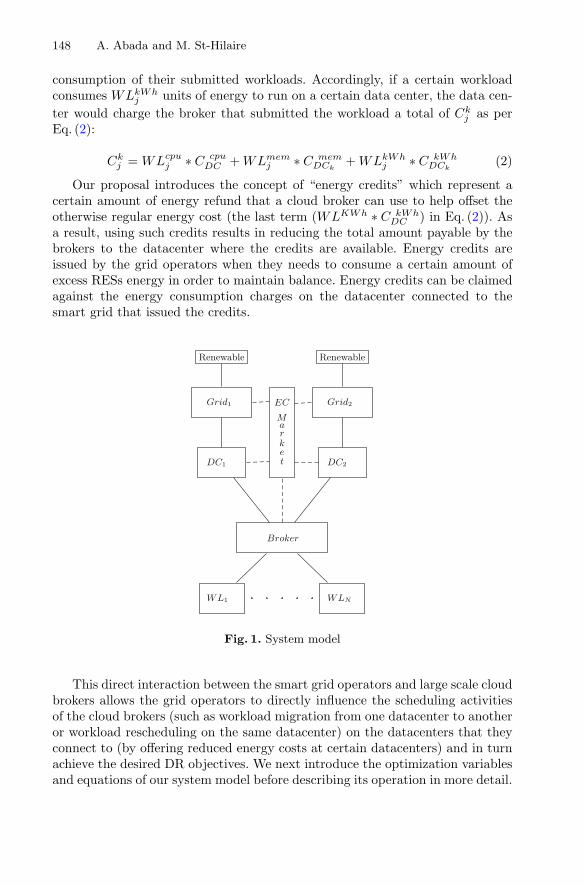
148 A. Abada and M. St-Hilaire
consumption of their submitted workloads. Accordingly, if a certain workloadconsumes WLkWh
j units of energy to run on a certain data center, the data cen-ter would charge the broker that submitted the workload a total of Ck
j as perEq. (2):
Ckj = WLcpu
j ∗ C cpuDC + WLmem
j ∗ C memDCk
+ WLkWhj ∗ C kWh
DCk(2)
Our proposal introduces the concept of “energy credits” which represent acertain amount of energy refund that a cloud broker can use to help offset theotherwise regular energy cost (the last term (WLKWh ∗ C kWh
DC ) in Eq. (2)). Asa result, using such credits results in reducing the total amount payable by thebrokers to the datacenter where the credits are available. Energy credits areissued by the grid operators when they needs to consume a certain amount ofexcess RESs energy in order to maintain balance. Energy credits can be claimedagainst the energy consumption charges on the datacenter connected to thesmart grid that issued the credits.
Renewable Renewable
Grid1 Grid2
DC1 DC2
Broker
WL1 WLN
EC
Market
Fig. 1. System model
This direct interaction between the smart grid operators and large scale cloudbrokers allows the grid operators to directly influence the scheduling activitiesof the cloud brokers (such as workload migration from one datacenter to anotheror workload rescheduling on the same datacenter) on the datacenters that theyconnect to (by offering reduced energy costs at certain datacenters) and in turnachieve the desired DR objectives. We next introduce the optimization variablesand equations of our system model before describing its operation in more detail.
Renewable Energy Curtailment 149
CcpuB the cost that broker B charges for the processing capacity allocated
per time slot (in $/FLOPS)Cmem
B the cost that broker B charges for disk-space usage per time slot (in$/MB)
Anextjk a binary variable that is set to 1 if job j is assigned to data center k
in the next time slotAcurrent
jk a binary variable that is set to 1 if job j is assigned to data center kin the current time slot (initial value = 0)
UECjk a binary variable that indicates if job j can claim energy creditsavailable at data center k
M the number of available data centersC cpu
DCkthe processing cost at datacenter k per time slot allocated (in$/FLOPS)
C memDCk
the disk-space cost at datacenter k per time slot allocated (in $/MB)CkWh
DCkthe price of energy at datacenter k (in $/kWh)
ECk the number of energy credits available at data center k (in kWh)MigCostkl a normalized value in the range of [0,1] that represents the cost
of migrating data from datacenter k to datacenter l (distance-based)
CapcpuDCkthe maximum processing capacity of datacenter k (in FLOPS)
CapmemDCk
the maximum disk-storage capacity at datacenter k (in MB)N the number of client workloads that needs to be assigned to data
centersWLcpu
j the processing capacity needed to process the workload of job j (inFLOPS)
WLmemj the amount of disk storage needed to host the workload of job j (in
MB)WLkWh
j the energy consumption of job j per each time slot allocated to it(in kWh)
Ljk a normalized value (between 0.8–1) that represents the latencybetween request j and datacenter k. (distance-based)
max
M∑
k=1
⎛
⎝N∑
j=1
([WL
memj ∗ C
memB + WL
cpuj ∗ C
cpuB
]∗ Ljk ∗ A
nextjk
)⎞
⎠ (3)
−M∑
k=1
⎛
⎝N∑
j=1
([WL
memj ∗ C
memDCk
+ WLcpuj ∗ C
cpuDCk
+ WLKWhj ∗ C
kWHDCk
]∗ A
nextjk
)⎞
⎠ (4)
+
M∑
k=1
⎛
⎝N∑
j=1
(UECjk ∗ WL
KWhj ∗ C
kWHDCk
)⎞
⎠ (5)
−M∑
k=1
⎛
⎝N∑
j=1
(UECjk ∗ WL
KWhj ∗ 0.1 C
kWHDCk
)⎞
⎠ (6)
−N∑
j=1
(M∑
k=1
Acurrentjk
(M∑
l=1
Anextjl ∗ MigCost[k][l] ∗ WL
memj
))(7)
150 A. Abada and M. St-Hilaire
s.t.
N∑
j=1
(WLKWh
j ∗ UECjk
)< ECk, ∀k ∈ M (8)
M∑
k=1
Anextjk ≤ 1, ∀j ∈ N (9)
UECjk <= Anextjk , ∀j ∈ N, k ∈ M (10)
N∑
j=1
WLcpuj ∗ Anext
jk ≤ Capcpuk , ∀k ∈ M (11)
N∑
j=1
WLmemj ∗ Anext
jk ≤ Capmemk , ∀k ∈ M (12)
We assume that the cloud broker continuously receives end-user requests(workloads) of different processing (WLcpu), storage (WLmem) and energy con-sumption (WLkWh) weights and that it needs to find the most cost efficientallocation for the received workloads on the available data centers in order tomaximize its revenue. We also assume that each workload and data center inthe system is associated with a location coordinate (x, y) that is used to deter-mine the distance-based latency Ljk between a workload j and a data center kas well as the migration cost factor MigCost[k][l] between data centers k andl. We consider that time is divided into discrete time intervals of equal dura-tion and that the cloud broker needs to decide a cost efficient allocation for itsworkloads at the beginning of each interval. We further assume that the pricingcoefficients of the cloud broker (Ccpu
B and CmemB ) remain fixed over all allocation
intervals while the pricing coefficients of the different data centers (C cpuDC , C cpu
DC
and C cpuDC ) do change (within a certain range) from one interval to another in
order to simulate a dynamic datacenter pricing and allow the broker to adjustits workload allocation on each interval according to the new prices in order tomaximize its revenue. We also assume that the cost of purchasing energy cred-its can be any fraction of the regular price as dictated by the EC market andconsider several example values for this fraction (0.1, 0.4 and 0.7) in our resultssection to show the effect of this parameter on our model. This allows the brokerto have enough incentive to reschedule/migrate its workloads in order to takeadvantage of the low cost energy and balance the grid in the process.
Our optimization formulation introduced above seeks to maximize the finan-cial gain of the cloud broker subject to system constraints. This optimizationis evaluated by the cloud broker at the beginning of each allocation interval inorder to decide which data center each of its workloads should be assigned toand whether the allocated workload can benefit from using energy credits or not.
The decision variables of our optimization model are the matrices Anextjk
and UECjk introduced earlier. Anextjk represents the allocation/assignment result
of the broker’s workloads (incoming requests) on the different available datacenters, whereas UECjk on the other hand represents whether each workload iscounted towards the consumption of energy credits at the datacenters that the
Renewable Energy Curtailment 151
workloads were assigned to (when such credits are available). Our optimizationformulation seeks to choose the appropriate values for Anext
jk and UECjk suchthat the objective function is maximized. Assuming that the cloud broker needsto assign a total of N workload requests, each to one of the M available datacenters, the above decision variables Anext
jk and UECjk can then be representedas two 2-dimensional boolean matrices of size [N ][M ] where each element Ajk
(s.t. j ∈ N and k ∈ M) is assigned the value of “1” if workload j was assignedto be hosted on data center k in the next allocation interval and “0” otherwise.Similarly, each element UECjk is assigned the value of “1” if workload j iscounted towards the consumption of the energy credits available at data centerk in the next allocation interval and “0” otherwise.
Using Anextjk and UECjk as the decision variables in the above optimization
formulation, the objective function tries to maximize the financial gain of thecloud broker given the different cost coefficients (Ccpu
DC , CmemDC , CkWH
DC ) of theM available data centers and the weights (WLcpu, WLmem, WLkWh) of the Nworkloads that needs to be assigned. The net financial gain is estimated as thesum of total generated revenues (represented with a “+” sign in the objectivefunction) minus the sum of total costs (represented with a “−” sign in theobjective function). The first term (3) in the objective function represents themoney that the cloud broker generates from its clients in exchange for hostingtheir workloads on the different data centers. If a workload WLj was successfullyassigned to be hosted on a data center k (i.e. Anext
jk = 1), that workload is saidto be generating revenue in the amount shown by the first term of the objectivefunction. The whole first term is multiplied by a scaling-down factor Ljk thatranges between [0.8, 1] and represents the distance-based latency between aworkload j and data center k where as the distance between a workload and adata center increases, Ljk will decrease to approach (0.8). The purpose of scalingdown the first term by Ljk is to enforce the cloud broker to favor assigningworkloads to data centers that are geographically closer to them in order tominimize the latency. The second term (4) of the objective function representsthe money that the cloud broker would need to pay to the data center that theworkload was assigned to. It is simply the weights of the workload multiplied bythe corresponding cost at the data center and finally multiplied by the allocationdecision variable Anext
jk . The third term (5) of the objective function representsthe regular value of the used energy credits if they were to be bought at theregular price. The fourth term (6) is the actual (reduced) cost price paid foracquiring the energy credits. Accordingly, the difference between the third andfourth terms (actual and reduced costs) represents a monetary gain that thecloud broker achieves by using the reduced cost energy credits offered by thesmart grid. The last term (7) of the objective function represents the cost ofmigrating a workload of size WLmem from data center k to data center l. Forthis term, we utilize the [M ]× [M ] size MigCost matrix that contains distance-based migration cost factors between the different data centers. Migration costfactors range from [0, 1] and approach the value of 0 as the distance betweendata centers gets closer. In order to detect a migration event we use Acurrent
jk to

152 A. Abada and M. St-Hilaire
hold the allocation results from the previous iteration and we detect a migrationif for a workload WLj we have Acurrent
jk = 1 and Anextjl = 1 and k �= l.
The first optimization constraint (8) states that the total weight of workloadsthat can claim usage of energy credits on a data center may not exceed the totalamount of energy credits available on that data center. The second constraint(9) limits the number of data center assignments that a workload can get toa maximum of “1”, since we assume that workloads can only be assigned to amaximum of one datacenter at a time. The third constraint (10) ensures thata workload has to be assigned to a data center in order for it to be countedtowards the energy credits consumption at that data center (i.e. energy creditscan not be claimed at a certain data center if the workload is not assigned tobe hosted there). The fourth and fifth constraints (11), (12) are data centercapacity constraints to ensure that each data center does not get assigned moreworkloads than what its capacity can accommodate.
4 Performance Analysis
Since our request/workload assignment problem is essentially a multidimensionalbinpacking problem where each request is defined by three dimensions (cpu,memory and kWh), the computational complexity of our problem is known tobe NP-Hard [32]. Therefore, we have implemented our system model using twoapproaches, first, as a linear optimization problem into the CPLEX ILP solverand second, using the more scalable approach of the Best Fit Decreasing (BFD)assignment heuristic, so we can evaluate our model under the two implemen-tations. In this section we present our simulation results that measures twodifferent aspects related to our model, namely the effect of the amount of energycredits introduced in the system on the time needed to balance a certain amountof excess energy and the effect of the amount of introduced energy credits onthe revenue generated by a cloud broker. We used a system model consistingof three data centers and a single cloud broker as discussed before to maintainsystem simplicity. Time is modeled in discrete intervals of equal size and theCPLEX/BFD implementations are ran by the broker at the beginning of eachinterval to determine the allocation/mapping of the requests/workloads on thedifferent available datacenters. Our shown simulation results are the averages of100 randomized runs where the cost coefficients (Cmem
DC , CcpuDC , CkWH
DC ) and loca-tion coordinates of all data centers are randomized (within the specified rangesas shown in Table 1) at the beginning of each allocation interval in order tomimic a dynamic cost system that would require the broker to optimize/adjustits workload allocations at the beginning of each new interval and induce work-load migrations between data centers. We have set the range of the datacenterenergy consumption cost parameter CkWH
DC slightly higher than the other dat-acenter costs in order to make datacenters with available energy credits moreattractive as hosts. On the other hand, the cloud broker adopts fixed cost coef-ficients (Cmem
B , CcpuB ) over all allocation intervals in order to shield its clients
from the uncertainty of the volatile live pricing model applied by datacenters.
Renewable Energy Curtailment 153
The fixed costs of the broker are set higher than the randomized datacenter coststo allow it to still make profit under any cost applied by the datacenters. We alsoshow the effect of variable system loads on the measured parameters by usingdifferent workload arrival rates (10, 20, 30, 40, 50 new request per allocationinterval) for each simulation. The list of the different parameters used in ourperformance testing are listed in Table 1.
Table 1. Simulation parameters
Parameter Min Max
CmemDC , Ccpu
DC 5 15
CkWHDC 25 30
CmemB , Ccpu
B 100 100
WLmem, WLcpu, WLkwh 5 15
WLduration 3 5
Available energy credits (EC) 0 3000
Workload arrival rate 10 50
Datacenter CPU capacity 5000 5000
Datacenter memory capacity 5000 5000
Figure 2 shows the effect of using different cost fractions (0.1, 0.4 and 0.7)for energy credits prices on the time needed to balance the grid given that acertain amount of energy needs to be consumed. Here we assume that 3000units of energy needs to be consumed by a datacenter in order to balance thegrid and we observe how long it takes (in number of allocation intervals) thedatacenter to consume this amount when different cost fractions of the originalprice are offered as energy credits. We notice that reducing the price of offeredenergy credits always speeds up the time needed for grid balancing especiallyunder light system loads as the workloads quickly become concentrated at thedata center that has the energy credits. We also notice that both CPLEX andBFD perform almost exactly the same in all simulated cases. This is due tothe big size difference between the request/workload size requirements and thecapacity of datacenters (as shown in Table 1), which is a valid assumption inmost realistic situations. Because request sizes are considerably smaller thandatacenter capacities and the fact that the BFD algorithm always orders theitems in a decreasing fashion before assignment, BFD can achieve as optimalbinpacking results as CPLEX except for the last “critical element” that getsrejected for size capacity violations. Therefore, the size of the last element thatgets rejected from a bin represents an upper bound on the efficiency of thebin assignment. This upper bound is minimized under the assumption of smallrequest sizes. Figure 3 shows the effect of using different cost fractions (0.1, 0.4and 0.7) for energy credits prices on the broker’s generated revenues. We cansee that the generated revenues increase as the cost fraction of energy credits

154 A. Abada and M. St-Hilaire
Fig. 2. Effect of varying ECs cost onbalancing time
Fig. 3. Effect of varying ECs cost onBroker’s profit
decrease. This is expected as energy credits represent discounted energy costsand the lower the cost paid towards acquiring the energy credits the more profitsare generated.
5 Conclusion and Future Work
Effective grid balancing is essential for ensuring the reliable operation of modernsmart grids. In this work we presented a new linear optimization approach thatuses energy credits as an incentive to control the energy consumption levels oflarge scale datacenter clients (such as cloud brokers/colocation tenant) for gridbalancing purposes. Simulations performed on our optimization model using
Renewable Energy Curtailment 155
two different implementation approaches showed that using energy credits asan incentive can speed up the grid balancing process and increases the brokersprofit margins. In future work we plan to expand the proposed system to includemultiple cloud brokers to compete for the available energy credits by way of gametheory bidding mechanism in order to maximize the smart grid’s return on theoffered energy credits.
References
1. Wang, J., Botterud, A., Bessa, R., Keko, H., Carvalho, L., Issicaba, D., Sumaili,J., Miranda, V.: Wind power forecasting uncertainty and unit commitment. Appl.Energy 88(11), 4014–4023 (2011)
2. Nicolosi, M.: Wind power integration and power system flexibility-an empiricalanalysis of extreme events in Germany under the new negative price regime. EnergyPolicy 38(11), 7257–7268 (2010). Energy Efficiency Policies and Strategies withregular papers
3. Olson, A., Jones, R.A., Hart, E., Hargreaves, J.: Renewable curtailment as a powersystem flexibility resource. Electr. J. 27(9), 49–61 (2014)
4. Khuri, S., Schutz, M., Heitkotter, J.: Evolutionary heuristics for the bin packingproblem. In: Pearson, D.W., Steele, N.C., Albrecht, R.F. (eds.) Artificial NeuralNets and Genetic Algorithms, pp. 285–288. Springer, Vienna (1995). https://doi.org/10.1007/978-3-7091-7535-4 75
5. Albadi, M.H., El-Saadany, E.F.: Demand response in electricity markets: anoverview. In: 2007 IEEE Power Engineering Society General Meeting, pp. 1–5,June 2007
6. Basmadjian, R., Lovasz, G., Beck, M., Meer, H.D., Hesselbach-Serra, X., Botero,J.F., Klingert, S., Ortega, M.P., Lopez, J.C., Stam, A., Krevelen, R.V., Giro-lamo, M.D.: A generic architecture for demand response: the ALL4Green approach.In: 2013 International Conference on Cloud and Green Computing, pp. 464–471,September 2013
7. Spees, K., Lave, L.B.: Demand response and electricity market efficiency. Electr.J. 20(3), 69–85 (2007)
8. Chen, H., Caramanis, M.C., Coskun, A.K.: The data center as a grid load stabilizer.In: 2014 19th Asia and South Pacific Design Automation Conference (ASP-DAC),pp. 105–112, January 2014
9. Chis, A., Rajasekharan, J., Lunden, J., Koivunen, V.: Demand response for renew-able energy integration and load balancing in smart grid communities. In: 2016 24thEuropean Signal Processing Conference (EUSIPCO), pp. 1423–1427, August 2016
10. Kim, H., Kim, Y.J., Yang, K., Thottan, M.: Cloud-based demand response forsmart grid: architecture and distributed algorithms. In: 2011 IEEE InternationalConference on Smart Grid Communications (SmartGridComm), pp. 398–403,October 2011
11. Wierman, A., Liu, Z., Liu, I., Mohsenian-Rad, H.: Opportunities and challengesfor data center demand response. In: International Green Computing Conference,pp. 1–10, November 2014
12. Schomaker, G., Janacek, S., Schlitt, D.: The energy demand of data centers. In:Hilty, L.M., Aebischer, B. (eds.) ICT Innovations for Sustainability. AISC, vol. 310,pp. 113–124. Springer, Cham (2015). https://doi.org/10.1007/978-3-319-09228-7 6

156 A. Abada and M. St-Hilaire
13. Rong, H., Zhang, H., Xiao, S., Li, C., Hu, C.: Optimizing energy consumption fordata centers. Renew. Sustain. Energy Rev. 58, 674–691 (2016)
14. Ferreto, T.C., Netto, M.A., Calheiros, R.N., Rose, C.A.D.: Server consolidationwith migration control for virtualized data centers. Future Gener. Comput. Syst.27(8), 1027–1034 (2011)
15. Varasteh, A., Goudarzi, M.: Server consolidation techniques in virtualized datacenters: a survey. IEEE Syst. J. 11(2), 772–783 (2017)
16. Van, H.N., Tran, F.D., Menaud, J.M.: SLA-aware virtual resource management forcloud infrastructures. In: 2009 Ninth IEEE International Conference on Computerand Information Technology, vol. 1, pp. 357–362, October 2009
17. Wu, C.M., Chang, R.S., Chan, H.Y.: A green energy-efficient scheduling algorithmusing the DVFS technique for cloud datacenters. Future Gener. Comput. Syst. 37,141–147 (2014)
18. Buchbinder, N., Jain, N., Menache, I.: Online job-migration for reducing the elec-tricity bill in the cloud. In: Domingo-Pascual, J., Manzoni, P., Palazzo, S., Pont, A.,Scoglio, C. (eds.) NETWORKING 2011. LNCS, vol. 6640, pp. 172–185. Springer,Heidelberg (2011). https://doi.org/10.1007/978-3-642-20757-0 14
19. Rao, L., Liu, X., Xie, L., Liu, W.: Minimizing electricity cost: optimization ofdistributed internet data centers in a multi-electricity-market environment. In:2010 Proceedings IEEE INFOCOM, pp. 1–9, March 2010
20. Chiu, D., Stewart, C., McManus, B.: Electric grid balancing through lowcost work-load migration. SIGMETRICS Perform. Eval. Rev. 40(3), 48–52 (2012)
21. Bollen, M.: The Smart Grid: Adapting the Power System to New Challenges.Morgan and Claypool, San Rafael (2011)
22. Vos, K.D.: Negative wholesale electricity prices in the German, French and Belgianday-ahead, intra-day and real-time markets. Electr. J. 28(4), 36–50 (2015)
23. Brandstatt, C., Brunekreeft, G., Jahnke, K.: How to deal with negative powerprice spikes?—flexible voluntary curtailment agreements for large-scale integrationof wind. Energy Policy 39(6), 3732–3740 (2011)
24. Kane, L., Ault, G.: A review and analysis of renewable energy curtailment schemesand principles of access: transitioning towards business as usual. Energy Policy 72,67–77 (2014)
25. Subramanian, A., Bitar, E., Khargonekar, P., Poolla, K.: Market induced curtail-ment of wind power. In: 2012 IEEE Power and Energy Society General Meeting,pp. 1–8, July 2012
26. Kavanagh, R., Armstrong, D., Djemame, K., Sommacampagna, D., Blasi, L.:Towards an energy-aware cloud architecture for smart grids. In: Altmann, J.,Silaghi, G.C., Rana, O.F. (eds.) GECON 2015. LNCS, vol. 9512, pp. 190–204.Springer, Cham (2016). https://doi.org/10.1007/978-3-319-43177-2 13
27. Zhang, S., Ran, Y., Wu, X., Yang, J.: Electricity cost optimization for data centersin smart grid environment. In: 11th IEEE International Conference on ControlAutomation (ICCA), pp. 290–295, June 2014
28. https://www.rackspace.com/managed-hosting/colocation29. Ren, S., Islam, M.A.: Colocation demand response: why do i turn off my servers?
In: 11th International Conference on Autonomic Computing (ICAC 2014), pp.201–208. USENIX Association, Philadelphia (2014)
30. Zhan, Y., Ghamkhari, M., Xu, D., Mohsenian-Rad, H.: Propagating electricitybill onto cloud tenants: using a novel pricing mechanism. In: 2015 IEEE GlobalCommunications Conference (GLOBECOM), pp. 1–6, December 2015

Renewable Energy Curtailment 157
31. Zhan, Y., Ghamkhari, M., Xu, D., Ren, S., Mohsenian-Rad, H.: Extending demandresponse to tenants in cloud data centers via non-intrusive workload flexibilitypricing. IEEE Trans. Smart Grid 99, 1–1 (2016)
32. Christensen, H.I., Khan, A., Pokutta, S., Tetali, P.: Approximation and onlinealgorithms for multidimensional bin packing: a survey. Comput. Sci. Rev. 24, 63–79 (2017)

Pricing Cloud Resource Basedon Reinforcement Learning
in the Competing Environment
Bing Shi1,2(B), Hangxing Zhu1, Han Yuan1, Rongjian Shi1, and Jinwen Wang1
1 School of Computer Science and Technology, Wuhan University of Technology,Wuhan, People’s Republic of China
[email protected] State Key Laboratory for Novel Software Technology, Nanjing University,
Nanjing, People’s Republic of China
Abstract. Multiple cloud providers compete against each other in orderto attract cloud users and make profits in the cloud market. In doing so,each provider needs to charge fees to users in a proper way. In this paper,we will analyze how a cloud provider sets price effectively when compet-ing against other cloud providers. Specifically, we model this problem asa Markov game, and then use minimax-Q and Q learning algorithms todesign the pricing policies respectively. Based on this, we run extensiveexperiments to analyze the effectiveness of minimax-Q and Q learningbased pricing policies. We find that although minimax-Q is more suit-able in analyzing the competing game with multiple self-interested cloudproviders, Q learning based pricing policy performs better in terms ofmaking profits. We also find that minimax-Q learning based pricing pol-icy performs better in terms of keeping cloud users. Our experimentalresults can provide useful insights on designing practical pricing policiesin different situations.
Keywords: Competing cloud providers · Pricing policyReinforcement learning · Minimax-Q learning
1 Introduction
During the past few years, the development of cloud computing has achievedsignificant success in the industry since it can provide economical, scalable, andelastic access to computing resources, thus liberating people from installing,configuring, securing, and updating a variety of hardware and software [1–3].More and more firms and personal users have been using cloud computing ser-vices over Internet, which contribute to the development of the cloud computingmarket. The global cloud computing market is expected to grow at a 30% com-pound annual growth rate (CAGR) reaching $270 billion in 2020. To competefor hundreds of billions of dollars, many firms as service providers have been
c© Springer International Publishing AG, part of Springer Nature 2018M. Luo and L.-J. Zhang (Eds.): CLOUD 2018, LNCS 10967, pp. 158–171, 2018.https://doi.org/10.1007/978-3-319-94295-7_11

Pricing Cloud Resource Based on Reinforcement Learning 159
participating in the cloud market [4]. Now, there exist many dominating cloudplatforms offering cloud services, such as Microsoft’s Azure, IBM’s SoftLayerand Amazon’s AWS. In the cloud market with multiple cloud providers, cloudusers have various choices, and they usually participate in the provider whichcan satisfy their demands and charge the lowest price to them. Actually, whenmultiple providers offer similar quality of service [5–7], the price will significantlyaffect users’ choices and thus providers’ profits. Therefore, cloud providers needto set effective prices to compete against each other. Furthermore, the compe-tition among providers usually lasts for a long time, i.e. the providers competeagainst each other repeatedly, and thus they need to maximize the long-termprofits. In this paper, we will analyze how a cloud provider designs an appropri-ate pricing policy to maximize the long-term profit and also remain attractiveto cloud users.
There exist some works on designing pricing policies for cloud providers. In[8], a non-cooperative competing model based on game theory has been pro-posed which computes the equilibrium price for one-shot game and does notconsider the long-term profits. In [9,10], the authors assume that there is onlyone provider, while in today’s cloud market multiple providers exist and competeagainst each other. Then the authors in [11,12] analyze the user behavior withrespect to the providers’ prices, but ignore the competition among providers. In[13], the authors analyze the pricing policy in the competing environment byassuming that there is only one proactive provider, and other providers just fol-low the proactive one’s pricing policy. Some other works, such as [14,15], considerthe competition among providers but does not capture the market dynamics, andtheir algorithms can only be applied to a very small market with few users.
To the best of our knowledge, few works have considered the situation ofmultiple providers competing against each other repeatedly. In this paper, we willanalyze how the competing cloud provider sets price effectively to maximize thelong-term profits in the context with two competing providers.1 In more detail,we first describe basic settings of cloud users and providers. Specifically, weconsider the uncertainty of users choosing cloud providers in the setting, whichis consistent with the realistic user behavior. Furthermore, how users choosingcloud providers is affected by the prices, and how cloud providers setting pricesis affected by users’ choices, and therefore it is a sequential-decision problem.Moreover, this problem involves two self-interested cloud providers, and thus itis a Markov game [16]. In this paper, we model the competition between cloudproviders as a Markov game, and then use two typical reinforcement learningalgorithms, minimax-Q learning [17] and Q learning [18], to solve this gameand design the pricing policy. We then run extensive experiments to evaluatethe policies in different situations. We find that although minimax-Q learning,which was specifically designed for Markov games, is more suitable to be appliedin this issue, Q learning based pricing policy performs better in terms of makingprofits. We also find that minimax-Q based pricing policy is better for remainingattractive to cloud users.
1 Our model can be easily extended to the case with more than two cloud providers.
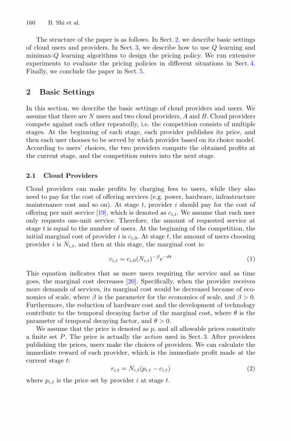
160 B. Shi et al.
The structure of the paper is as follows. In Sect. 2, we describe basic settingsof cloud users and providers. In Sect. 3, we describe how to use Q learning andminimax-Q learning algorithms to design the pricing policy. We run extensiveexperiments to evaluate the pricing policies in different situations in Sect. 4.Finally, we conclude the paper in Sect. 5.
2 Basic Settings
In this section, we describe the basic settings of cloud providers and users. Weassume that there are N users and two cloud providers, A and B. Cloud providerscompete against each other repeatedly, i.e. the competition consists of multiplestages. At the beginning of each stage, each provider publishes its price, andthen each user chooses to be served by which provider based on its choice model.According to users’ choices, the two providers compute the obtained profits atthe current stage, and the competition enters into the next stage.
2.1 Cloud Providers
Cloud providers can make profits by charging fees to users, while they alsoneed to pay for the cost of offering services (e.g. power, hardware, infrastructuremaintenance cost and so on). At stage t, provider i should pay for the cost ofoffering per unit service [19], which is denoted as ci,t. We assume that each useronly requests one-unit service. Therefore, the amount of requested service atstage t is equal to the number of users. At the beginning of the competition, theinitial marginal cost of provider i is ci,0. At stage t, the amount of users choosingprovider i is Ni,t, and then at this stage, the marginal cost is:
ci,t = ci,0(Ni,t)−βe−θt (1)
This equation indicates that as more users requiring the service and as timegoes, the marginal cost decreases [20]. Specifically, when the provider receivesmore demands of services, its marginal cost would be decreased because of eco-nomics of scale, where β is the parameter for the economics of scale, and β > 0.Furthermore, the reduction of hardware cost and the development of technologycontribute to the temporal decaying factor of the marginal cost, where θ is theparameter of temporal decaying factor, and θ > 0.
We assume that the price is denoted as p, and all allowable prices constitutea finite set P . The price is actually the action used in Sect. 3. After providerspublishing the prices, users make the choices of providers. We can calculate theimmediate reward of each provider, which is the immediate profit made at thecurrent stage t:
ri,t = Ni,t(pi,t − ci,t) (2)
where pi,t is the price set by provider i at stage t.

Pricing Cloud Resource Based on Reinforcement Learning 161
2.2 Cloud Users
Each user has a marginal value on per-unit requested service, which is denotedas δ. At stage t, after all providers publish the prices, user j can calculate itsexpected revenue when entering provider i, which is:
Rtj,i = δj − pi,t (3)
Intuitively, based on Eq. 3, cloud users can determine in which provider they canobtain the maximal revenue at the current stage, and then choose that provider.However, in the real world, users keep requiring cloud services, and they usuallytake into account the prices at previous stages. Specifically, in this paper, weassume that the users will consider the prices at the current stage t and the laststage t − 1 when choosing the cloud providers. We do not need to consider theprices at all previous stages since in this paper, the providers’ prices and theusers’ choices are affected by each other, and thus the price of the last stageactually implies the dynamic interaction of all previous stages. Therefore, theexpected utility that user j can make when entering provider i is:
vtj,i = ξRt
j,i + (1 − ξ)Rt−1j,i (4)
where ξ is the weight of the price considered by the user at this stage. Further-more, in reality, when agents make decisions, their choices are affected by someunobservable factors [21], such as customers’ loyalty on some product brand,which is denoted as ηj,i. This part introduces the uncertainty of users’ choice.Now the utility that cloud user j makes in provider i at stage t is defined asfollows:
utj,i = vt
j,i + ηj,i (5)
We assume that the random variable ηj,i is an independently, identically dis-tributed extreme value, i.e. it follows Gumbel and type I extreme value distri-bution [21], and the density of ηj,i is
f(ηj,i) = e−ηj,ie−e−ηj,i (6)
and the cumulative distribution is
F (ηj,i) = e−e−ηj,i (7)
The probability of user j choosing provider i at stage t, which is denoted asP t
j,i
P tj,i = Prob(ut
j,i > utj,i′ ,∀i′ �= i)
= Prob(vtj,i + ηj,i > vt
j,i′ + ηj,i′ ,∀i′ �= i)
= Prob(ηj,i′ < ηj,i + vtj,i − vt
j,i′ ,∀i′ �= i) (8)
According to (7), P tj,i is
P tj,i = e−e
(ηj,i+vtj,i−vt
j,i′ )(9)
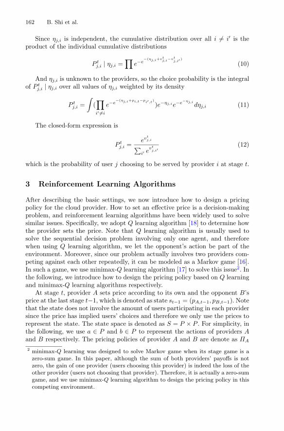
162 B. Shi et al.
Since ηj,i is independent, the cumulative distribution over all i �= i′ is theproduct of the individual cumulative distributions
P tj,i | ηj,i =
∏e−e
−(ηj,i+vtj,i−vt
j,i′ )(10)
And ηj,i is unknown to the providers, so the choice probability is the integralof P t
j,i | ηj,i over all values of ηj,i weighted by its density
P tj,i =
∫(∏
i′ �=i
e−e−(ηj,i+pi,t−p
i′,t)
)e−ηj,ie−e−ηj,idηj,i (11)
The closed-form expression is
P tj,i =
evtj,i
∑i′ e
vtj,i′
(12)
which is the probability of user j choosing to be served by provider i at stage t.
3 Reinforcement Learning Algorithms
After describing the basic settings, we now introduce how to design a pricingpolicy for the cloud provider. How to set an effective price is a decision-makingproblem, and reinforcement learning algorithms have been widely used to solvesimilar issues. Specifically, we adopt Q learning algorithm [18] to determine howthe provider sets the price. Note that Q learning algorithm is usually used tosolve the sequential decision problem involving only one agent, and thereforewhen using Q learning algorithm, we let the opponent’s action be part of theenvironment. Moreover, since our problem actually involves two providers com-peting against each other repeatedly, it can be modeled as a Markov game [16].In such a game, we use minimax-Q learning algorithm [17] to solve this issue2. Inthe following, we introduce how to design the pricing policy based on Q learningand minimax-Q learning algorithms respectively.
At stage t, provider A sets price according to its own and the opponent B’sprice at the last stage t−1, which is denoted as state st−1 = (pA,t−1, pB,t−1). Notethat the state does not involve the amount of users participating in each providersince the price has implied users’ choices and therefore we only use the prices torepresent the state. The state space is denoted as S = P × P . For simplicity, inthe following, we use a ∈ P and b ∈ P to represent the actions of providers Aand B respectively. The pricing policies of provider A and B are denote as ΠA
2 minimax-Q learning was designed to solve Markov game when its stage game is azero-sum game. In this paper, although the sum of both providers’ payoffs is notzero, the gain of one provider (users choosing this provider) is indeed the loss of theother provider (users not choosing that provider). Therefore, it is actually a zero-sumgame, and we use minimax-Q learning algorithm to design the pricing policy in thiscompeting environment.

Pricing Cloud Resource Based on Reinforcement Learning 163
Algorithm 1. Q learningInput: pricing space P ; B’s pricing policy ΠB
Output: A’s pricing policy ΠA
1: for ∀s ∈ S, V (s) = 0, and ∀a ∈ P, Q(s, a) = 02: for ∀s ∈ S, ∀a ∈ P, ΠA(s, a) = 1/|P |3: repeat4: at the current state s, given ε, generate a random number rand (0 < rand < 1);
when rand ≤ ε, A chooses a price a ∈ P randomly; when rand > ε, A chooses aprice a ∈ P according to the pricing policy ΠA
5: B chooses the price b (according to the pricing policy ΠB), the next state iss′ = (a, b)
6: Q(s, a) = (1 − α) ∗ Q(s, a) + α ∗ (ri,t + γ ∗ V (s′))7: ΠA(s, ·) = argmaxΠ′
A(s,·)(
∑a′(ΠA(s, a′) ∗ Q(s, a′)))
8: V (s) =∑
a(ΠA(s, a) ∗ Q(s, a))9: until (ΠA(s, ·) is converged)
Algorithm 2. minimax-Q learningInput: pricing space P ; B’s pricing policy ΠB
Output: A’s pricing policy ΠA
1: for ∀s ∈ S, V (s) = 0, and ∀a ∈ P, Q(s, a, b) = 02: for ∀s ∈ S, ∀a ∈ P, ΠA(s, a) ← 1/|P |3: repeat4: at the current state s, given ε, generate a random number rand (0 < rand < 1);
when rand ≤ ε, A chooses a price a ∈ P randomly; when rand > ε, A chooses aprice a ∈ P according to the pricing policy ΠA
5: B chooses the price b (according to the pricing policy ΠB), the next state iss′ = (a, b)
6: Q(s, a, b) = (1 − α) ∗ Q(s, a, b) + α ∗ (ri,t + γ ∗ V (s′))7: ΠA(s, ·) = argmaxΠ′
A(s,·)(minb′
∑a′(ΠA(s, a′) ∗ Q(s, a′, b′)))
8: V (s) = minb′(∑
a′(ΠA(s′, a′) ∗ Q(s′, a′, b′)))9: until (ΠA(s, ·) is converged)
and ΠB respectively. Based on these notations, Q learning algorithm is shownin Algorithm 1, and minimax-Q learning algorithm is shown in Algorithm 2. Inthis setting, it is guaranteed that both algorithms will converge [17,18]. The finaloutput ΠA is the designed pricing policy.
4 Experimental Analysis
In this section, we run numerical simulations to analyze the reinforcement learn-ing based pricing policies in different situations. We first describe the parametersetup in the experiments in the following.

164 B. Shi et al.
Table 1. Experimental parameters
Parameter setup Description
c.,0 = 5 cloud provider’s marginal cost at the initial stage
P = {10, 20, . . . , 100} the set of allowable prices
N = 100 the amount of users in the market
δ ∈ [50, 150] the cloud user’s marginal value δ follows a uniformdistribution supported on [50,150]
β = 0.01 parameter β in Eq. 1
θ = 0.001 parameter θ in Eq. 1
ξ = 0.8 parameter ξ in Eq. 4
ε = 0.2 exploration rate in Q learning and minimax-Q learningalgorithms
γ = 0.8 discount factor in Q learning and minimax-Q learningalgorithms
4.1 Experimental Parameters
First, we assume that each cloud provider has the same initial marginal cost,i.e. c.,0 = 5, and the marginal cost is decreased as the demand increases. Inaddition, we assume that the set of allowable prices P chosen by cloud providersis {10, 20, . . . , 100}. Furthermore, we assume that there are N = 100 cloud usersin total. The marginal values of users δ are independent random variable, and forillustrative purpose, we assume that they are drawn from a uniform distributionwith support [50, 150]. Other parameters used in the following simulations followthe typical setting in the related literature, and are shown in Table 1.
4.2 Pricing Policy
We first describe the pricing policies trained and output by minimax-Q and Qlearning algorithms respectively. We consider the case that the cloud providertakes Q learning and minimax-Q learning algorithms against the opponent choos-ing actions randomly, and the case that both cloud providers are trained in Qlearning and minimax-Q learning algorithms. We name the trained pricing poli-cies as QR,QQ,MR and MM respectively, and for example QQ means thatboth cloud providers adopt Q learning algorithm and are trained against eachother. We show these four pricing policies in Fig. 1. From these figures, we canfind the probability of the provider choosing each price (action) at each state.Note that in this paper, the state is a tuple including two providers’ prices atthe last stage, and in order to show the state in one-dimension state-axis, wemap state (10, 10) to 1, map state (10, 20) to 2, ......, map (20, 10) to 11, ......,and map (100, 100) to 100. Furthermore, we find that no provider intends to
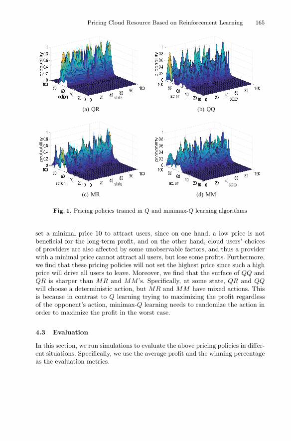
Pricing Cloud Resource Based on Reinforcement Learning 165
(a) QR (b) QQ
(c) MR (d) MM
Fig. 1. Pricing policies trained in Q and minimax-Q learning algorithms
set a minimal price 10 to attract users, since on one hand, a low price is notbeneficial for the long-term profit, and on the other hand, cloud users’ choicesof providers are also affected by some unobservable factors, and thus a providerwith a minimal price cannot attract all users, but lose some profits. Furthermore,we find that these pricing policies will not set the highest price since such a highprice will drive all users to leave. Moreover, we find that the surface of QQ andQR is sharper than MR and MM ’s. Specifically, at some state, QR and QQwill choose a deterministic action, but MR and MM have mixed actions. Thisis because in contrast to Q learning trying to maximizing the profit regardlessof the opponent’s action, minimax-Q learning needs to randomize the action inorder to maximize the profit in the worst case.
4.3 Evaluation
In this section, we run simulations to evaluate the above pricing policies in differ-ent situations. Specifically, we use the average profit and the winning percentageas the evaluation metrics.

166 B. Shi et al.
(a) Average profit
(b) Winning percentage
Fig. 2. MM , MR, QQ, QR vs. Random
vs. Random Pricing Policy. We first evaluate these four pricing policiesagainst the opponent adopting a random pricing policy, which chooses eachprice with equal probability. The reason for doing this is that when participat-ing in the cloud market, some fresh cloud providers often explore the competingenvironment randomly in order to collect more market information. The com-peting results are shown in Fig. 2, where Fig. 2(a) is the average profit over 10000stages, and Fig. 2(b) is the winning percentage of these four policies competingagainst the random pricing policy. We find that all these four pricing policy canbeat the opponent. Not surprisingly, we find that QR is the best one amongthese four policies when competing against the random pricing policy since QRis trained specifically against the random policy. In contrast, we find that MRis the worst one. This is because when the opponent chooses the price randomly,i.e. not trying to make the other side be the worst, minimax-Q cannot performwell. In fact, we find that QQ and QR perform better than MR and MM . Thismay indicate that the agent should adopt Q learning when its opponent cannottake action in an intelligent way.

Pricing Cloud Resource Based on Reinforcement Learning 167
(a) Average profit
(b) Winning percentage
Fig. 3. MM, MR, QQ, QR vs. Linear Reduction
vs. Price Reduction Policy. In the real world, cloud providers usually attractcloud users by decreasing the price continuously. For example, when a fresh cloudprovider enters the market, it may keep decreasing the price to attract users. Wealso evaluate these four pricing policies against the cloud provider which keepsreducing the price. Specifically, we consider two typical price reduction poli-cies, Linear Reduction and Exp Reduction. In Linear Reduction policy, the pricedecreases linearly with respect to time, where at stage t the price is pt = p0−0.01t(p0 is the initial price, and we set it as the maximal price, i.e. 100), while in ExpReduction, the price decreases exponentially with time, where pt = p0 ∗e−0.0003t
(p0 = 100 which is the same as before). The results of QQ,QR,MM,MR com-peting against Linear Reduction policy and Exp Reduction policy are shown inFigs. 3 and 4. We still find that our reinforcement learning-based pricing policiescan beat these price reduction policies. Again, we find that MM and MR cannotoutperform the reduction policies significantly than that QQ and QR do.
Q-X vs. X. In the above, it seems that when competing against the oppo-nent using simple pricing policies (i.e. random or price reduction), Q learningbased pricing policy is better. However, after investigating the fundamentals ofminimax-Q and Q learning algorithms, we can see that minimax-Q is more suit-able in this Markov game with two competing providers. Since this is not provedin the above experiments, in the following we further investigate this issue by

168 B. Shi et al.
(a) Average profit
(b) Winning percentage
Fig. 4. MM, MR, QQ, QR vs. Exp Reduction
using Q learning algorithm to train the pricing policy against the above fourpolicies, i.e. QQ,QR,MR,MM . We then obtained four new pricing policies, Q-QR, Q-QQ, Q-MR, and Q-MM . Q-QR is a pricing policy based on Q learningcompeting against QR pricing policy in the above section. We run the followingsimulations including Q-MM vs MM , Q-MR vs MR, Q-QQ vs QQ and Q-QRvs QR. The results are shown in Fig. 5, where QQ,QR,MR,MM are denoted asX. From Fig. 5(b), in terms of winning percentage, we find that Q-QQ outper-forms QQ and Q-QR outperforms QR, i.e. the winning percentage is more than50%. However, even though Q-MM is trained against MM , it is outperformedby MM , i.e. the winning percentage is less than 50%. The similar result happensfor Q-MR. However, from Fig. 5(a), we find that even though Q-MM is out-performed by MM in terms of winning percentage, it obtains more profits thanMM . It is similar for Q-MR. This is because minimax-Q based pricing policiestry to do the best in the worst case, and therefore its winning percentage canbe kept at a good level. However, Q learning based policies try to maximize theprofits at all times, and therefore perform better in terms of making profits.

Pricing Cloud Resource Based on Reinforcement Learning 169
(a) Average profit
(b) Winning percentage
Fig. 5. Q-X vs. X
5 Conclusions
How to set prices effectively is an important issue for the cloud provider, espe-cially in the environment with multiple cloud providers competing against eachother. In this paper, we use reinforcement learning algorithms to address thisissue. Specifically, we model the issue as a Markov game, and use minimax-Qand Q learning algorithms to design the pricing policies respectively. We thenrun extensive experiments to analyze the pricing policies. We find that althoughminimax-Q is more suitable in analyzing the competing game with multiple self-interested agents, Q learning based pricing policy performs better in terms ofmaking profits. We also find that minimax-Q based pricing policy is better forremaining attractive to cloud users. The experimental results can provide usefulinsights on designing practical pricing policies in different situations.
Acknowledgment. This paper was funded by the National Natural Science Founda-tion of China (No. 61402344), the Excellent Dissertation Cultivation Funds of WuhanUniversity of Technology (No. 2017-YS-065) and the Fundamental Research Funds forthe Central Universities (WUT:2017II14XZ).

170 B. Shi et al.
References
1. Armbrust, M., Fox, A., Griffith, R., Joseph, A.D., Katz, R., Konwinski, A., Lee,G., Patterson, D., Rabkin, A., Stoica, I., Zaharia, M.: A view of cloud comput-ing: clearing the clouds away from the true potential and obstacles posed by thiscomputing capability. Commun. ACM 53(4), 50–58 (2010)
2. Buyya, R., Yeo, C.S., Venugopal, S., Broberg, J., Brandicl, I.: Cloud computingand emerging it platforms: vision, hype, and reality for delivering computing asthe 5th utility. Future Gener. Comput. Syst. 25(6), 599–616 (2009)
3. Foster, I., Zhao, Y., Raicu, I., Lu, S.: Cloud computing and grid computing 360-degree compared. In: Grid Computing Environments Workshop, pp. 1–10 (2008)
4. Buyya, R., Yeo, C., Venugopal, S.: Market-oriented cloud computing: vision, hype,and reality for delivering it services as computing utilities. In: The 10th IEEEInternational Conference on High Performance Computing and Communications,pp. 5–13 (2008)
5. Laatikainen, G., Ojala, A., Mazhelis, O.: Cloud services pricing models. In:Herzwurm, G., Margaria, T. (eds.) ICSOB 2013. LNBIP, vol. 150, pp. 117–129.Springer, Heidelberg (2013). https://doi.org/10.1007/978-3-642-39336-5 12
6. Sharma, B., Thulasiram, R.K., Thulasiraman, P., Garg, S.K., Buyya, R.: Pric-ing cloud compute commodities: a novel financial economic model. In: The 12thIEEE/ACM International Symposium on Cluster, Cloud and Grid Computing, pp.451–457 (2012)
7. Wang, H., Jing, Q., Chen, R., He, B., Qian, Z., Zhou, L.: Distributed systems meeteconomics: pricing in the cloud. In: The 2nd USENIX Conference on Hot Topicsin Cloud Computing, pp. 1–6 (2010)
8. Feng, Y., Li, B., Li, B.: Price competition in an oligopoly market with multipleiaas cloud providers. IEEE Trans. Comput. 63(1), 59–73 (2014)
9. Kantere, V., Dash, D., Francois, G., Kyriakopoulou, S., Ailamaki, A.: Optimalservice pricing for a cloud cache. IEEE Trans. Knowl. Data Eng. 23(9), 1345–1358(2011)
10. Xu, H., Li, B.: Maximizing revenue with dynamic cloud pricing: the infinite horizoncase. In: IEEE International Conference on Communications, pp. 2929–2933 (2012)
11. Vengerov, D.: A gradient-based reinforcement learning approach to dynamic pric-ing in partially-observable environments. Future Gener. Comput. Syst. 24(7), 687–693 (2008)
12. Xu, H., Li, B.: Dynamic cloud pricing for revenue maximization. IEEE Trans.Cloud Comput. 1(2), 158–171 (2013)
13. Xu, B., Qin, T., Qiu, G., Liu, T.Y.: Optimal pricing for the competitive and evo-lutionary cloud market. In: The 24th International Joint Conference on ArtificialIntelligence, pp. 139–145 (2015)
14. Truong-Huu, T., Tham, C.K.: A game-theoretic model for dynamic pricing andcompetition among cloud providers. In: The 6th International Conference on Utilityand Cloud Computing, pp. 235–238 (2013)
15. Truong-Huu, T., Tham, C.K.: A novel model for competition and cooperationamong cloud providers. IEEE Trans. Cloud Comput. 2(3), 251–265 (2014)
16. Wal, J.: Stochastic dynamic programming. Methematisch Centrum (1980)17. Littman, M.L.: Markov games as a framework for multi-agent reinforcement learn-
ing. In: 11th International Conference on Machine Learning, pp. 157–163 (1994)18. Watkins, C.J.C.H., Dayan, P.: Q-learning. Mach. Learn. 8(3–4), 279–292 (1992)

Pricing Cloud Resource Based on Reinforcement Learning 171
19. Adams, I.F., Long, D.D.E., Miller, E.L., Pasupathy, S., Storer, M.W.: Maximizingefficiency by trading storage for computation. In: The 1st USENIX Conference onHot Topics in Cloud Computing. vol. 7 (2009)
20. Jung, H., Klein, C.M.: Optimal inventory policies under decreasing cost functionsvia geometric programming. Eur. J. Oper. Res. 132(3), 628–642 (2001)
21. Train, K.E.: Discrete Choice Methods with Simulation. Cambridge UniversityPress, Cambridge (2003)

An Effective Offloading Trade-Offto Economize Energy and Performance
in Edge Computing
Yuting Cao, Haopeng Chen(B), and Zihao Zhao
Shanghai Jiao Tong University, Dongchuan Rd., Shanghai, China{seniyuting,chen-hp,1059198449}@sjtu.edu.cn
Abstract. Mobile Edge Computing is a new technology which aimsto reduce latency, to ensure highly efficient network operation and tooffer an improved user experience. Considering offloading will introduceadditional wireless transmission overhead, the key technical challenge ofmobile edge computing is tradeoff between computation cost and wirelesstransmission cost, reducing energy consumption of mobile edge devicesand response time of computation task at the same time. A Mobile EdgeComputing System composed of Mobile Edge Device and Edge Cloud,connecting with Wireless Stations, comes out. To protect user privacy,Data Preprocessing is proposed which includes irrelevant property cleanand data segmentation. Aimed at reducing total energy consumptionand response time, an energy consumption priority offloading (ECPO)algorithm and a response time priority offloading (RTPO) algorithmare put forward, based on Energy Consumption Model and ResponseTime Model. Combining both ECPO and RTPO, a dynamic comput-ing offloading algorithm is raised which is more universal. Finally, sim-ulations in four scenarios, including network normal scenario, networkcongested scenario, device low battery scenario and task time limitedscenario, demonstrate that our algorithms can effectively reduce energyconsumption of mobile edge device and response time of computationtask.
Keywords: Mobile edge computing · ECPO · RTPO · Offloading
1 Introduction
With the rapid development of Internet of Things [1], mobile edge devices gener-ate a lot of data, performing as not only data consumers but also data producers[2]. Under this circumstance, traditional cloud computing is no longer a wisechoice since it has some obvious drawbacks. Firstly, it is not acceptable for realtime computation task on mobile edge devices because bandwidth of networkwould be the bottleneck. Secondly, user privacy is another problem to be solvedfor cloud computing.
c© Springer International Publishing AG, part of Springer Nature 2018M. Luo and L.-J. Zhang (Eds.): CLOUD 2018, LNCS 10967, pp. 172–186, 2018.https://doi.org/10.1007/978-3-319-94295-7_12

An Effective Offloading Trade-Off to Economize Energy and Performance 173
Mobile Edge Computing is a new technology which provides an IT serviceenvironment and cloud computing capabilities at the edge of mobile network,within the Radio Access Network and in close proximity to mobile subscribers.The aim is to reduce latency, to ensure highly efficient network operation andservice delivery, and to offer an improved user experience [3]. In mobile edgecomputing scenario, network latency can be reduced by enabling computationand storage capacity at the edge network. And mobile edge devices can per-form computation offloading for computing intensive applications to leveragethe context-aware mobile edge computing service by using real time radio accessnetwork information [4]. Since offloading introduces additional communicationoverhead, a key technical challenge is how to balance between computation costand communication cost to support applications with enhanced user experience,such as lower response time and energy consumption [5].
In this paper, we design a Mobile Edge Computing System composed ofMobile Edge Device and Edge Cloud, connecting with Wireless Station. To pro-tect user privacy, Data Preprocessing is proposed including irrelevant propertyclean and data segmentation. Assuming that horizontal segmentation of inputdata will not affect computing result and execution time of computing is pro-portional to data size, input data can be divided into multiple data blocks anddata block can be divided into multiple data slices with fixed data size. Onlyone data slice can be executed each time. In our research, we focus on reducingenergy consumption of mobile edge device and response time of computationtask, proposing an Energy Consumption Model and a Response Time Model.
In terms of mobile edge computing offloading problem, considering the changeof network environment and the power of mobile edge device to make a dynamicdecision will work better than making an unchanging decision at the beginning.Therefore, an energy consumption priority offloading (ECPO) algorithm and aresponse time priority offloading (RTPO) algorithm are raised in order to reduceenergy consumption and response time. Furthermore, combining both ECPOalgorithm and RTPO algorithm, we propose a new dynamic computing offload-ing algorithm as the greatest contribution of our paper. Finally, simulations infour scenarios: network normal scenario, network congested scenario, device lowbattery scenario and task time limited scenario, demonstrate that our proposedalgorithms can effectively reduce energy consumption and response time.
The structure of this paper is as follows. Section 2 presents the related work.Section 3 describes system design and system model. In Sect. 4, we proposeECPO alogorithm, RTPO algorithm and a dynamic computing offloading algo-rithm combining previous two. Section 5 shows the simulation results and anal-ysis. Section 6 is about conclusion and future work.
2 Related Work
Recently, computing offloading from mobile devices into cloud [6], as a key tech-nical challenge of Mobile Edge Computing [7], has been extensively studied inmany area including power management [8], cloud computing task migration[9,10] and virtual machine migration [11].

174 Y. Cao et al.
In order for better understanding of offloading, Orsini et al. provide a designguideline for the selection of suitable concepts for different classes of commoncloud-augmented mobile applications and present open issues that developersand researchers should be aware of when designing their mobile cloud computingapproach [12].
There are some existing offloading algorithms, like energy-optimal partialcomputation offloading (EPCO) algorithm [5], Lyapunov optimization-baseddynamic computation offloading (LODCO) algorithm [13], distributed computa-tion offloading algorithm [14] and the actor-model programming paradigm [15].Sardellitti et al. consider an MIMO multicell system where multiple mobile usersask for computation offloading to a common cloud server and propose an iter-ative algorithm, based on a novel successive convex approximation technique,converging to a local optimal solution of original nonconvex problem [16].
In order to save energy, Zhao et al. design a threshold-based policy to improvethe QoS of Mobile Cloud Computing by cooperation of local cloud and Inter-net cloud resources, which takes advantages of low latency of local cloud andabundant computational resources of Internet cloud simultaneously [17]. Ge etal. propose a game-theoretic approach to optimize the overall energy in a mobilecloud computing system and formulate the energy minimization problem as acongestion game, where each mobile device is a player to select one server tooffload computation to minimize the overall energy consumption [18]. Wangand Giannakis investigate resource allocation policies for time-division multipleaccess over fading channels in the power-limited regime [19].
What’s more, Chen et al. study the multi-user computation offloading prob-lem for mobile-edge cloud computing in a multi-channel wireless interferenceenvironment and design a distributed computation offloading algorithm thatcan achieve a Nash equilibrium, deriving the upper bound of the convergencetime and quantifying its efficiency ratio over the centralized optimal solutionin terms of two important performance metrics [14]. You et al. study resourceallocation for a multiuser MECO system based on time-division multiple access(TDMA) and orthogonal frequency-division multiple access (OFDMA) to solvethe problem and characterize its policy structure, proposing a low-complexitysub-optimal algorithm by transforming the OFDMA problem to its TDMA coun-terpart [20].
3 System Design and System Model
In this section, we introduce system architecture design and data preprocess-ing method. The energy consumption model and response time model are alsopresented. Partial parameters used in the following are listed in Table 1.
3.1 System Architecture Design
The system is composed of two requisite parts: Mobile Edge Device and EdgeCloud, while data transmission of them is Wireless Station. The system archi-tecture is shown in Fig. 1.
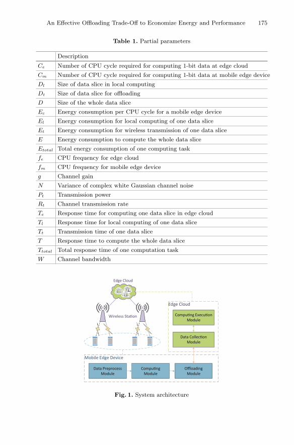
An Effective Offloading Trade-Off to Economize Energy and Performance 175
Table 1. Partial parameters
Description
Ce Number of CPU cycle required for computing 1-bit data at edge cloud
Cm Number of CPU cycle required for computing 1-bit data at mobile edge device
Dl Size of data slice in local computing
Dt Size of data slice for offloading
D Size of the whole data slice
Ec Energy consumption per CPU cycle for a mobile edge device
El Energy consumption for local computing of one data slice
Et Energy consumption for wireless transmission of one data slice
E Energy consumption to compute the whole data slice
Etotal Total energy consumption of one computing task
fe CPU frequency for edge cloud
fm CPU frequency for mobile edge device
g Channel gain
N Variance of complex white Gaussian channel noise
Pt Transmission power
Rt Channel transmission rate
Te Response time for computing one data slice in edge cloud
Tl Response time for local computing of one data slice
Tt Transmission time of one data slice
T Response time to compute the whole data slice
Ttotal Total response time of one computation task
W Channel bandwidth
Edge Cloud
Compu ng Execu onModule
Data Collec on Module
Mobile Edge Device
Data Preprocess Module
OffloadingModule
Compu ngModule
Wireless Sta on
Edge Cloud
Fig. 1. System architecture

176 Y. Cao et al.
Mobile Edge Device. Mobile Edge Device is both data consumer and dataproducer in edge computing, including three modules: Data Preprocess Module,Computing Module and Offloading Module. Data Preprocess Module is respon-sible for irrelevant property clean and data segmentation. Computing Moduleis used for local computing. Offloading Module is used to develop calculationmigration strategy.
Edge Cloud. There are two modules in Edge Cloud: Computing ExecutionModule and Data Collection Module. Computing Execution Module is a modulethat performs computational tasks, while Data Collection Module is applied forcollecting data from Mobile Edge Device.
3.2 Data Preprocessing
There are two kinds of data preprocessing: Irrelevant Property Clean and DataSegmentation. On the one hand, the original data may contain some propertieswhich are related to user private and computing irrelevant. On the other hand, inthe case of horizontal segmentation of input data not affecting computing result,we propose to segment from multiple granularities on the basic definition of DataUnit, smallest data processing unit for performing computational tasks. DataUnit can be divided into multiple Data Blocks while Data Block can be dividedinto multiple Data Slices as shown in Fig. 2. The purpose of multi-granularitydata segmentation is to dynamically adjust the computing migration mechanismfor different granularity data which will be analyzed in Sect. 4.
DataSlice
DataSlice
DataSlice
DataSlice
DataSlice
Data Unit
DataSlice
Data Block Data Block
Fig. 2. Data segmentation
3.3 Energy Consumption Model
One of the main purposes of mobile edge computing is to reduce energy consump-tion of mobile edge devices as much as possible, including energy consumptionfor local computing and for wireless transmission.

An Effective Offloading Trade-Off to Economize Energy and Performance 177
Energy Consumption for Local Computing. For a mobile edge device,let Ec denote the energy consumption per CPU cycle for local computing, Cm
denote the number of CPU cycles required for computing 1-bit of input dataand Dl denote the size of data slice. Then the total energy consumption for localcomputing of a data slice is El, given by Formula 1.
El = Cm · Dl · Ec (1)
Energy Consumption for Wireless Transmission. Let W denote the chan-nel bandwidth, g denote the channel gain, Pt denote the transmission powerand N denote the variance of complex white Gaussian channel noise. Then thechannel transmission rate denoted by Rt, is Formula 2, according to Shannonformula.
Rt = W · log2(1 +g · Pt
W · N ) (2)
Provided that W , Pt and N are constant, Rt will have a positive correla-tion with changeable g. However, if time slot is short enough, Pt and Rt canbe considered constant, resulting to the total energy consumption for wirelesstransmission of a data slice as Et, given by Formula 3, where Tt and Dt aretransmission time and size of offloading data slice respectively.
Et = Pt · Tt =Pt · Dt
Rt(3)
By the way, energy consumption for wireless transmission of calculation resultis negligible in this case due to size of result is much smaller than that of originaldata normally.
Total Energy Consumption. Considering the size of data slice is smallenough, the local computing time and transmission time of data slice is short.Under this circumstances, analysis of energy consumption is acceptable.
Let D denote size of the whole data slice, Dl denote the size of data slicein local computing with 0 ≤ Dl ≤ D, then the size of offloading data slice isDt = D − Dl. Total energy consumption denoted as E is given by Formula 4.
E = El + Et =Pt
Rt· D + (Cm · Ec − Pt
Rt) · Dl (4)
For the case of Cm ·Ec− Pt
Rt> 0, E will be minimum when Dl = 0. Oppositely,
supposing Cm · Ec − Pt
Rt≤ 0, E will be minimum when Dl = D. It shows that
for a data slice small enough, to make energy consumption minimum, the wholedata slice is either executed in local computing or offloaded to edge cloud.
The total energy consumption of one computation task can be expressed asFormula 5.
Etotal =∑
Eslice, for each data slice (5)

178 Y. Cao et al.
3.4 Response Time Model
Another purpose of mobile edge computing is to reduce computing response time,which is mainly affected by three factors: local computing, wireless transmissionand cloud computing.
Response Time for Local Computing. For a mobile edge device, let fmdenote CPU frequency for local computing which means the number of CPUcycles per second, Cm denote the number of CPU cycles required for computing1-bit data and Dl denote the size of data slice in local computing. Then the totalresponse time for local computing of a data slice is Tl, given by the followingFormula 6.
Tl =Cm · Dl
fm(6)
Response Time for Wireless Transmission. If the time slot is short enough,the channel transmission rate Rt can be considered to be constant. In this case,the total response time for wireless transmission of a data slice of input data isTt, given by Formula 7.
Tt =Dt
Rt=
D − Dl
Rt(7)
where Dt is the size of offloading data slice. Response time for wireless trans-mission of computing results is ignored due to the relative smaller sizes.
Response Time for Cloud Computing. Obviously in edge cloud, the CPUfrequency denoted as fe and the number of CPU cycles required for computing1-bit data denoted as Ce can be considered constant within a time slot which isshort enough. Then the total response time for cloud computing of a data sliceis Te, given by Formula 8.
Te =Ce · Dt
fe=
Ce · (D − Dl)fe
(8)
Total Response Time. For a data slice, local execution and offloading to edgecloud are simultaneous, which leads to the total response time be the maximumof them, given by Formula 9.
T = max(Tl, Tt + Te) (9)
Total response time of a computation task can be expressed as Formula 10.
Ttotal =∑
Tslice, for each data slice (10)

An Effective Offloading Trade-Off to Economize Energy and Performance 179
4 Computing Offloading Mechanism
Reducing energy consumption and response time is two main purpose for com-puting offloading mechanism in edge computing. In this section, we proposed anenergy consumption priority offloading algorithm named ECPO and a responsetime priority offloading algorithm named RTPO. Ultimately, we put forword adynamic computing offloading algorithm based on ECPO and RTPO.
4.1 Energy Consumption Priority Offloading Algorithm
To reduce the total energy consumption of mobile edge device, an energy con-sumption priority offloading (ECPO) algorithm is proposed in Algorithm 1.
Algorithm 1: ECPO AlgorithmInput: data: input data or data block
1 Divide data into data slices2 for each DataSlice do3 if DataSlice is non-offloadable then4 Execute DataSlice in local computing5 else6 Get connection information of wireless station7 Calculate Cm, Ec, Pt and Rt in Formula 48 Set Param = Cm · Ec − Pt/Rt
9 if Param > 0 then10 Offloading DataSlice to Edge Cloud11 else12 Execute DataSlice in local computing
As is shown in Fig. 3, in ECPO algorithm, data will be divided into multipledata slices with fixed data size under the assumption that horizontal segmenta-tion will not affect computing result. For each data slice, it will be either executedin local computing or offloaded to edge cloud. Only one data slice can be exe-cuted each time. What’s more, total energy consumption of one data slice E inECPO algorithm is shown in Formula 4. As is proved by Energy ConsumptionModel, E will be minimum when using ECPO algorithm.
4.2 Response Time Priority Offloading Algorithm
Considering that ECPO algorithm has space for improving response time ofcomputation task, an response time priority offloading (RTPO) algorithm isproposed in Algorithm 2.
As is shown in Fig. 4, in RTPO algorithm, the offloading weight of a dataslice is calculated according to the power percentage of mobile edge device and

180 Y. Cao et al.
Mobile Edge Device
DataSlice
Edge Cloud
DataSlice
Local Compu ng
offloading
Result Result DataSlice Result
Fig. 3. Energy consumption priority offloading
Algorithm 2: RTPO AlgorithmInput: data: input data or data block
1 Divide data into data slices2 for each DataSlice do3 if DataSlice is non-offloadable then4 Execute DataSlice in local computing5 else6 Get connection information of wireless station7 Calculate current channel transmission rate Rt
8 Dl = (fm · fe + Ce · fm ·Rt) ·D/(Cm · fe ·Rt + fm · fe + Ce · fm ·Rt)9 Execute local computing and offload to Edge Cloud at the same time
network status. In other words, RTPO algorithm allows one data slice to executeboth in local and edge cloud to earn less response time.
For each data slice, the response time for executing local computing to processa data unit is Cm
fm, while time for offloading to edge cloud is 1
Rt+ Ce
fe. So for a
data slice, in order to equalize this two latencies, we get the weight for localcomputing Dl in Formula 11. As is analyzed previously in Formula 4, totalenergy consumption of one data slice E in RTPO algorithm will not be theworst case as Dl always satisfy the condition 0 < Dl < D.
Dl =(fm · fe + Ce · fm · Rt) · D
Cm · fe · Rt + fm · fe + Ce · fm · Rt(11)
4.3 Dynamic Computing Offloading Algorithm
In order to deal with more complex scenarios, we propose a dynamic computingoffloading algorithm in Algorithm 3, combining ECPO and RTPO algorithm.
The dynamic computing offloading algorithm takes both power of mobile edgedevice and user requirements into consideration. On the one hand, if mobile edge
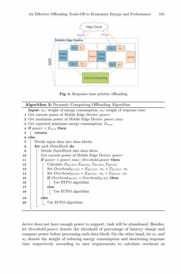
An Effective Offloading Trade-Off to Economize Energy and Performance 181
Mobile Edge Device
Edge Cloud
Local Compu ng
offloading
DataSlice Result
DS1
DS2
R1
R2
DataSlice Result
DS1
DS1
R1
R2
offloading
Fig. 4. Response time priority offloading
Algorithm 3: Dynamic Computing Offloading AlgorithmInput: we: weight of energy consumption, wt: weight of response time
1 Get current power of Mobile Edge Device: power2 Get maximum power of Mobile Edge Device: power max3 Get expected minimum energy consumption: Emin
4 if power < Emin then5 return6 else7 Divide input data into data blocks8 for each DataBlock do9 Divide DataBlock into data slices
10 Get current power of Mobile Edge Device: power11 if power > power max · threshold power then12 Calculate EECPO, ERTPO, TECPO, TRTPO
13 Set OverheadECPO = EECPO · we + TECPO · wt
14 Set OverheadRTPO = ERTPO · we + TRTPO · wt
15 if OverheadRTPO < OverheadECPO then16 Use RTPO algorithm17 else18 Use ECPO algorithm
19 else20 Use ECPO algorithm
device does not have enough power to support, task will be abandoned. Besides,let threshold power denote the threshold of percentage of battery charge andcompare power before processing each data block. On the other hand, let we andwt denote the weight of reducing energy consumption and shortening responsetime respectively according to user requirements to calculate overhead as

182 Y. Cao et al.
Formula 12. Finally, we select algorithm with lower overhead to deal with currentdata block.
Overhead = E · we + T · wt (12)
The energy consumption model and time model of one computaion task arethe sum of cost in each data block, which can be expressed as Formula 13.
Etotal =∑
Eblock, for each data block
Ttotal =∑
Tblock, for each data block
(13)
5 Evaluation
As 5G technology has not fully applied currently, it is scarcely possible to carryout experiments in real environment. In this section, we analyze our simula-tion result in four scenarios to evaluate performance of the proposed dynamiccomputing offloading mechanism, including network normal scenario, networkcongested scenario, device low battery scenario and task time limited scenario.
5.1 Experimental Parameter
Settings of our simulation are as follows. The size of data block and dataslice are 100 MB and 1 MB separately. Energy consumption per CPU cyclefor mobile edge device Ec = 1.0 × 10⁻¹⁰ J/cycle. The number of CPU cyclesrequired for computing 1-bit data at mobile edge device and edge cloud isCm = Ce = 1000 cycles/bits. CPU frequency for a mobile edge device is fm =2.0 × 10⁹ cycles/s while it for edge cloud is fe = 1.0 × 10¹⁰ cycles/s. Transmis-sion power is Pt ∈ [0, 0.2] J/s. Channel transmission rate is Rt ∈ [0, 2000] KB/s.Energy of mobile edge device at full charge is 20000 J and threshold power isset to 30%.
Moreover, as Formula 14 shows, WirelessStation consists of n channels andm devices are maintained for each channel, of which m has negative correlationof the wireless transmission rate.
WirelessStation(Channel1, Channel2, ..., Channeln−1, Channeln)Channel(Device1,Device2, ...,Devicem−1,Devicem)
(14)
Assuming that NumberChannel and NumberDevice represent the number ofchannels and mobile edge devices severally, we define the ratio of NumberChannel
and NumberDevice equalizing 20 as congested network, while equalizing 2 asnormal network in our experiment.
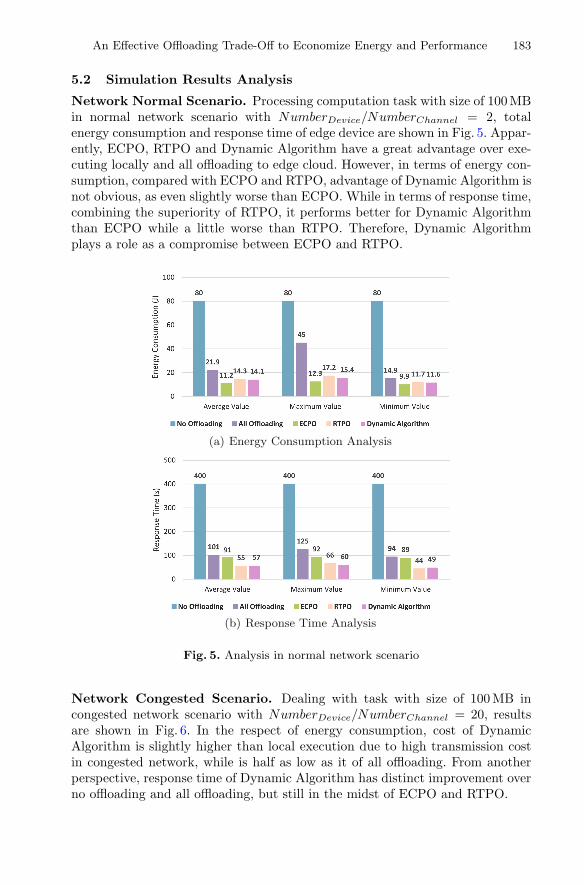
An Effective Offloading Trade-Off to Economize Energy and Performance 183
5.2 Simulation Results Analysis
Network Normal Scenario. Processing computation task with size of 100 MBin normal network scenario with NumberDevice/NumberChannel = 2, totalenergy consumption and response time of edge device are shown in Fig. 5. Appar-ently, ECPO, RTPO and Dynamic Algorithm have a great advantage over exe-cuting locally and all offloading to edge cloud. However, in terms of energy con-sumption, compared with ECPO and RTPO, advantage of Dynamic Algorithm isnot obvious, as even slightly worse than ECPO. While in terms of response time,combining the superiority of RTPO, it performs better for Dynamic Algorithmthan ECPO while a little worse than RTPO. Therefore, Dynamic Algorithmplays a role as a compromise between ECPO and RTPO.
(a) Energy Consumption Analysis
(b) Response Time Analysis
Fig. 5. Analysis in normal network scenario
Network Congested Scenario. Dealing with task with size of 100 MB incongested network scenario with NumberDevice/NumberChannel = 20, resultsare shown in Fig. 6. In the respect of energy consumption, cost of DynamicAlgorithm is slightly higher than local execution due to high transmission costin congested network, while is half as low as it of all offloading. From anotherperspective, response time of Dynamic Algorithm has distinct improvement overno offloading and all offloading, but still in the midst of ECPO and RTPO.

184 Y. Cao et al.
(a) Energy Consumption Analysis
(b) Response Time Analysis
Fig. 6. Analysis in Congested Network Scenario
Device Low Battery Scenario. The initial power of mobile edge device is setlower than 30% randomly in low battery scenario and the original data size ofeach task is 5 GB. Number of initial tasks is 100. Results of computing offloadingis shown in Table 2. The failure of computing tasks is due to exhaustion of mobileedge devices. Success rates of ECPO and RTPO are 91% and 75% each. DynamicAlgorithm will estimate energy consumption before executing tasks and abandoncalculation task when do not have enough power, resulting to 100% success rate.
Table 2. Result of computing offloading in device low battery scenario
Initialization Abandon Failure Success SuccessRate
ECPO 100 0 9 91 91%
RTPO 100 0 25 75 75%
Dynamic 100 10 0 90 100%

An Effective Offloading Trade-Off to Economize Energy and Performance 185
Task Time Limited Scenario The initial power of mobile edge device is setrandomly and the original data size of each task is 5 GB. Number of initial tasksis 100. In addition, each computing task is limited to 1 h. Results of computingoffloading is shown in Table 3. For ECPO, there are 2 tasks failed due to depletionof mobile edge devices, while the remaining 98% violate the time limit due totimeout. For RTPO, although its success rate is 95%, 5 tasks failed due toexhaustion of mobile edge device. For Dynamic Algorithm, success rate is 83%without failure which is optimal entirely.
Table 3. Result of computing offloading in task time limited scenario
Initialization Abandon Failure Timeout Punctuality SuccessRate
ECPO 100 0 2 98 0 0%
RTPO 100 0 5 0 95 95%
Dynamic 100 4 0 16 80 83%
5.3 Brief Summary
The simulation results conducted in 4 scenarios show that our computing offload-ing machanism can comprehensively consider energy consumption, response timeof computing tasks and load of edge cloud, by dynamically adjusting and calcu-lating offloading strategy. The machanism is far better than local execution andall offloading to edge cloud.
6 Conclusion
We study computing offloading mechanism for a mobile edge computing systemcomposed of mobile edge device and edge cloud, connecting with wireless station,to reduce energy consumption of mobile edge devices and response time of com-putation tasks. We propose ECPO and RTPO algorithm according to EnergyConsumption Model and Response Time Model. Ultimately, we put forward adynamic offloading algorithm combining the previous two, which is proved to bean effective way to achieve the original goals entirely. In the future, after fullapplication of 5G technology, we will make further effort to build a real mobileedge computing scenarios to verify the effectiveness of our mechanism.
References
1. Xia, F., Yang, L.T., Wang, L., Vinel, A.: Internet of Things. Int. J. Commun. Syst.25(9), 1101 (2012)
2. Shi, W., Dustdar, S.: The promise of edge computing. Computer 49(5), 78–81(2016)

186 Y. Cao et al.
3. Hu, Y.C., Patel, M., Sabella, D., Sprecher, N., Young, V.: Mobile edge computinga key technology towards 5G. ETSI White Pap. 11(11), 1–16 (2015)
4. Ahmed, A., Ahmed, E.: A survey on mobile edge computing. In: 2016 10th Inter-national Conference on Intelligent Systems and Control (ISCO), pp. 1–8 (2016)
5. Wang, Y., Sheng, M., Wang, X., Wang, L., Li, J.: Mobile-edge computing: par-tial computation offloading using dynamic voltage scaling. IEEE Trans. Commun.64(10), 4268–4282 (2016)
6. Kumar, K., Lu, Y.H.: Cloud computing for mobile users: can offloading computa-tion save energy? Computer 43(4), 51–56 (2010)
7. Dinh, H.T., Lee, C., Niyato, D., Wang, P.: A survey of mobile cloud computing:architecture, applications, and approaches. Wirel. Commun. Mob. Comput. 13(18),1587–1611 (2013)
8. Van, H.N., Tran, F.D., Menaud, J.M.: Performance and power management forcloud infrastructures. In: 2010 IEEE 3rd International Conference Cloud Comput-ing (CLOUD), pp. 329–336 (2010)
9. Chun, B.G., Ihm, S., Maniatis, P., Naik, M., Patti, A.: CloneCloud: elastic execu-tion between mobile device and cloud. In: Proceedings of the Sixth Conference onComputer Systems, pp. 301–314 (2011)
10. Kosta, S., Aucinas, A., Hui, P., Mortier, R., Zhang, X.: ThinkAir: dynamic resourceallocation and parallel execution in the cloud for mobile code offloading. In: INFO-COM, 2012 Proceedings IEEE, pp. 945–953 (2012)
11. Xiao, Z., Song, W., Chen, Q.: Dynamic resource allocation using virtual machinesfor cloud computing environment. IEEE Trans. Parallel Distrib. Syst. 24(6), 1107–1117 (2013)
12. Orsini, G., Bade, D., Lamersdorf, W.: Context-aware computation offloading formobile cloud computing: requirements analysis, survey and design guideline. Pro-cedia Comput. Sci. 56, 10–17 (2015)
13. Mao, Y., Zhang, J., Letaief, K.B.: Dynamic computation offloading for mobile-edgecomputing with energy harvesting devices. IEEE J. Sel. Areas Commun. 34(12),3590–3605 (2016)
14. Chen, X., Jiao, L., Li, W., Fu, X.: Efficient multi-user computation offloading formobile-edge cloud computing. IEEE/ACM Trans. Netw. 24(5), 2795–2808 (2016)
15. Haubenwaller, A.M., Vandikas, K.: Computations on the edge in the internet ofThings. Procedia Comput. Sci. 52, 29–34 (2015)
16. Sardellitti, S., Scutari, G., Barbarossa, S.: Joint optimization of radio and com-putational resources for multicell mobile-edge computing. IEEE Trans. Sig. Inf.Process. Netw. 1(2), 89–103 (2015)
17. Zhao, T., Zhou, S., Guo, X., Zhao, Y., Niu, Z.: A cooperative scheduling schemeof local cloud and internet cloud for delay-aware mobile cloud computing. In: 2015IEEE Globecom Workshops (GC Wkshps), pp. 1–6 (2015)
18. Ge, Y., Zhang, Y., Qiu, Q., Lu, Y.H.: A game theoretic resource allocation foroverall energy minimization in mobile cloud computing system. In: Proceedingsof the 2012 ACM/IEEE International Symposium on Low Power Electronics andDesign, pp. 279–284 (2012)
19. Wang, X., Giannakis, G.B.: Power-efficient resource allocation for time-divisionmultiple access over fading channels. IEEE Trans. Inf. Theory 54(3), 1225–1240(2008)
20. You, C., Huang, K., Chae, H., Kim, B.H.: Energy-efficient resource allocation formobile-edge computation offloading. IEEE Trans. Wirel. Commun. 16(3), 1397–1411 (2017)
Research Track: Cloud Management

Implementation and ComparativeEvaluation of an Outsourcing Approach
to Real-Time Network Servicesin Commodity Hosted Environments
Oscar Garcia1(B), Yasushi Shinjo1(B), and Calton Pu2(B)
1 Department of Computer Science, University of Tsukuba, Tsukuba, Ibaraki, [email protected], [email protected]
2 College of Computing, Georgia Institute of Technology, Atlanta, GA, [email protected]
Abstract. Commodity operating systems (OS) often sacrifice real-time(RT) performance (e.g., consistent low latency) in favor of optimizedaverage latency and throughput. This can cause latency variance prob-lems when an OS hosts virtual machines that run network services. Thispaper proposes a software-based RT method in Linux KVM-based hostedenvironments. First, this method solves the priority inversion problem ininterrupt handling of vanilla Linux using the RT Preempt patch. Sec-ond, this method solves another priority inversion problem in the softirqmechanism of Linux by explicitly separating the RT softirq handling fromthe non-RT softirq handling. Finally, this method mitigates the cachepollution problem by co-located non-RT services and avoids the secondpriority inversion in a guest OS by socket outsourcing. Compared to theRT Preempt Patch Only method, the proposed method has the 76%lower standard deviation, 15% higher throughput, and 33% lower CPUoverhead. Compared to the dedicated processor method, the proposedmethod has the 63% lower standard deviation, higher total throughputby a factor of 2, and avoids under-utilization of the dedicated processor.
1 Introduction
Large-scale applications with real-time (RT) or stringent quality of service (QoS)requirements, ranging from large distributed systems such as electronic trading,NextGen air traffic control [1], and web-facing e-commerce n-tier applications tosmall sensors and edge servers in Internet of Things (IoT), smart applicationsneed fast and consistent network services [2–6]. Owing to the variety of environ-ments in which these applications operate, there is a growing need for commodityoperating system (OS) with systematic improvements that can satisfy real-timeand stringent QoS performance requirements in both speed and consistency. Anindication of this trend is the number of real-time operating systems [7] thatbuild on commodity operating systems (Sect. 5).
c© Springer International Publishing AG, part of Springer Nature 2018M. Luo and L.-J. Zhang (Eds.): CLOUD 2018, LNCS 10967, pp. 189–205, 2018.https://doi.org/10.1007/978-3-319-94295-7_13
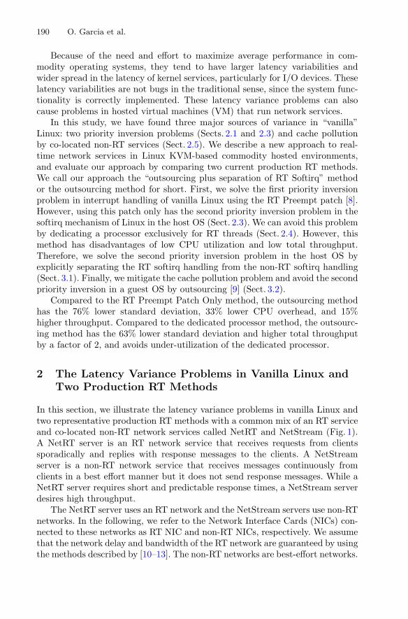
190 O. Garcia et al.
Because of the need and effort to maximize average performance in com-modity operating systems, they tend to have larger latency variabilities andwider spread in the latency of kernel services, particularly for I/O devices. Theselatency variabilities are not bugs in the traditional sense, since the system func-tionality is correctly implemented. These latency variance problems can alsocause problems in hosted virtual machines (VM) that run network services.
In this study, we have found three major sources of variance in “vanilla”Linux: two priority inversion problems (Sects. 2.1 and 2.3) and cache pollutionby co-located non-RT services (Sect. 2.5). We describe a new approach to real-time network services in Linux KVM-based commodity hosted environments,and evaluate our approach by comparing two current production RT methods.We call our approach the “outsourcing plus separation of RT Softirq” methodor the outsourcing method for short. First, we solve the first priority inversionproblem in interrupt handling of vanilla Linux using the RT Preempt patch [8].However, using this patch only has the second priority inversion problem in thesoftirq mechanism of Linux in the host OS (Sect. 2.3). We can avoid this problemby dedicating a processor exclusively for RT threads (Sect. 2.4). However, thismethod has disadvantages of low CPU utilization and low total throughput.Therefore, we solve the second priority inversion problem in the host OS byexplicitly separating the RT softirq handling from the non-RT softirq handling(Sect. 3.1). Finally, we mitigate the cache pollution problem and avoid the secondpriority inversion in a guest OS by outsourcing [9] (Sect. 3.2).
Compared to the RT Preempt Patch Only method, the outsourcing methodhas the 76% lower standard deviation, 33% lower CPU overhead, and 15%higher throughput. Compared to the dedicated processor method, the outsourc-ing method has the 63% lower standard deviation and higher total throughputby a factor of 2, and avoids under-utilization of the dedicated processor.
2 The Latency Variance Problems in Vanilla Linux andTwo Production RT Methods
In this section, we illustrate the latency variance problems in vanilla Linux andtwo representative production RT methods with a common mix of an RT serviceand co-located non-RT network services called NetRT and NetStream (Fig. 1).A NetRT server is an RT network service that receives requests from clientssporadically and replies with response messages to the clients. A NetStreamserver is a non-RT network service that receives messages continuously fromclients in a best effort manner but it does not send response messages. While aNetRT server requires short and predictable response times, a NetStream serverdesires high throughput.
The NetRT server uses an RT network and the NetStream servers use non-RTnetworks. In the following, we refer to the Network Interface Cards (NICs) con-nected to these networks as RT NIC and non-RT NICs, respectively. We assumethat the network delay and bandwidth of the RT network are guaranteed by usingthe methods described by [10–13]. The non-RT networks are best-effort networks.

Implementation and Comparative Evaluation of an Outsourcing Approach 191
In this figure, we run a network service in a VM. We allocate a single vCPUto each VM of NetStream, and the vCPU corresponds to a host thread with anormal priority. We allocate two vCPUs to the VM of NetRT. The first vCPU(non-RT vCPU) executes system tasks (e.g. housekeeping tasks) and it corre-sponds to a host thread with a normal priority. The second vCPU (RT vCPU)executes the NetRT server and it corresponds to a host thread with a high pri-ority. Each VM has a vNIC thread that executes a backend driver of the VMnetwork.
2.1 Interrupt Handling of Network Devices in Vanilla Linux
Linux implements the split interrupt handling model to handle interrupts.Figure 1a shows the interrupt handling in vanilla Linux. Each device driver of aNIC has two interrupt handlers: the hard IRQ handler and softirq handler. Thehard IRQ processes the essential interrupt tasks while interrupts are disabledand the softirq handler processes the remaining interrupt tasks including heavyTCP and bridge processing while interrupts are enabled.
Each CPU has an instance of the softirq mechanism and this instance isshared by multiple device drivers. To ensure cache affinity, the softirq handlerof a device driver is executed by the same CPU that receives the IRQ from thedevice and that executes the hard IRQ handler. The hard IRQ handler of a NICput the RT softirq handler into the poll list, which is the list of pending softirqhandlers in a per-CPU variable.
The interrupt handling in vanilla Linux has a priority inversion problem.Interrupt handlers are executed prior to user processes. For instance, in Fig. 1a,the RT vCPU thread, which is a high-priority user process, can be delayed bythe softirq handler of a non-RT NIC.
In this configuration, message copying is performed two times, i.e., oncebetween the host kernel and a guest kernel by a vNIC thread, and anotherfrom the guest kernel to a guest user process by a guest kernel. This messagecopying causes a cache pollution problem. We will discuss about it in Sect. 2.5.
2.2 The RT Preempt Patch Only Method
We can solve the priority inversion problem in Sect. 2.1 by using the RT Preemptpatch [8]. We call this method the RT Preempt Patch Only method. This patchmakes the kernel more preemptible by the following features:
– Hard IRQ handlers are executed as threads (IRQ threads).– Spin locks are translated into mutexes with a priority inheritance function.
Figure 1b shows that the threads of VMs and interrupt handlers in the RTPreempt Patch Only method. In this figure, each NIC has two IRQ threads fortwo CPUs. Each IRQ thread is bounded to a CPU.
This method solves the priority inversion problem in Sect. 2.1. Each IRQthread calls hard and softirq handlers with its own priority. In Fig. 1b, the IRQ

192 O. Garcia et al.
(a) Vanilla Linux (b) RT Preempt Patch Only
(c) Dedicated processor (d) Outsourcing
Fig. 1. Configurations of vanilla Linux and the RT methods.

Implementation and Comparative Evaluation of an Outsourcing Approach 193
Fig. 2. Priority inversion in interrupt handling of the host OS.
threads of the non-RT NICs do not preempt the threads of the RT VM. Thismethod can yield high achievable CPU utilization because all CPUs execute anyvCPU and vNIC threads.
2.3 The Priority Inversion in the Softirq Mechanism of Linux
The RT Preempt patch solves the priority inversion in Sect. 2.1. However, thereexists another type of priority inversion in the softirq mechanism of Linux.
Figure 2 shows a trace of the kernel activities using the RT Preempt PatchOnly method, where we obtained this plot using KernelShark [14]1. In this figure,while the CPU was executing the non-RT IRQ thread that called the non-RTsoftirq handler, the CPU received an interrupt from an RT NIC. The CPUactivated the RT IRQ thread, and called the RT hard IRQ handler. The RThard IRQ handler put the RT softirq handler into the poll list in a per-CPUvariable.
After finishing the RT hard IRQ handler, the RT IRQ thread entered thesoftirq mechanism. This thread tried to lock the per-CPU variable but it waslocked by the non-RT IRQ thread. Therefore, the CPU suspended the RT IRQthread and executed the non-RT IRQ thread. This thread continued the non-RTsoftirq handler. At this time, this thread ran with a high priority according tothe priority inheritance function. Therefore, the RT IRQ thread had to wait untilthe non-RT IRQ thread finished. This is a priority inversion.
Next, in Fig. 2, the non-RT softirq handler exceeded the execution quota.Therefore, the non-RT softirq handler was put at the end of the poll list. Next,the RT IRQ thread obtained the lock and called the RT softirq handler. Thishandler processed messages from the RT NIC, placed messages into a queue, andactivated the RT vNIC thread. Next, the RT IRQ thread also called the non-RTsoftirq handler with high priority, which created a priority inversion.
1 The results of KernelShark may include large probe effects.

194 O. Garcia et al.
2.4 Dedicated Processor Method
We can avoid the priority inversion in Sect. 2.3 by dedicating processors to RTthreads. This is a popular production method to run RT services in commodityhosted environments [15–18]. We call this method the dedicated processor method.
Figure 1c shows that this method allocates a group of RT threads to a ded-icated CPU. We call such a CPU an RT-CPU. In this method, an RT NICinjects interrupts to an RT-CPU and a non-RT NIC injects interrupts to a non-RT CPU. Interrupt handling of non-RT NICs do not disturb the execution ofthe RT threads.
While this method can achieve consistently low latency, it has a drawback.Because RT CPUs do not help to execute non-RT threads, this method yieldsless achievable CPU utilization.
2.5 Cache Pollution Problem
The CPUs (cores) of a system are explicitly-shared resources and we can controlthem through priorities of threads and dedication. On the other hand, the LastLevel Cache (LLC) is an implicitly-shared resource. When co-located non-RTservices pollute the LLC, this can interfere the execution of RT services. Forexample, in Fig. 1b, when the NetStream servers receive messages, vNIC threadsand guest operating systems copy these messages and this copying pollutes theLLC. This changes the response times of the NetRT server.
Note that we cannot avoid this problem using the dedicated processormethod. This is because in many CPU architectures, the LLC is shared amongCPU cores.
3 Outsourcing Method
Sections 2.2 and 2.4 described two production RT methods, the RT PreemptPatch only method and the dedicated processor method. This section shows ourproposed method, the outsourcing method.
Figure 1d shows the configuration of the method. This method is an extensionof the RT Preempt Patch Only method. It uses the RT Preempt patch and itassigns high priorities to RT threads. This method avoids the priority inversionin Sect. 2.3 by adding a new poll list for RT services as shown in Fig. 1d. Inaddition, this method mitigates the cache pollution problem in Sect. 2.5 andavoids the priority inversion in a guest OS by RT socket outsourcing.
3.1 Adding an RT Poll list for RT Services
In the outsourcing method, we divide the poll list of the softirq mechanism intotwo lists.
– The poll list for non-RT NIC handlers (the non-RT poll list).– The poll list for RT NIC handlers (the RT poll list).

Implementation and Comparative Evaluation of an Outsourcing Approach 195
Fig. 3. Separating RT interrupt handling from non-RT interrupt handling.
Figure 3 shows interrupt handling in the outsourcing method. While the CPUwas executing the non-RT softirq handler, the CPU received an interrupt froman RT NIC as in Fig. 2. The CPU activated the RT IRQ thread, and called theRT hard IRQ handler. The RT hard IRQ handler placed the RT softirq handlerinto the RT poll list.
After finishing the RT hard IRQ handler, the RT IRQ thread entered thesoftirq mechanism. This thread obtained the lock of the per-CPU variable andcalled the RT softirq handler. In contrast to the RT Preempt Patch Only method,it called the RT softirq handler and it did not call the non-RT softirq handlerbecause the RT poll list only contained the RT softirq handler. After the RTIRQ thread finished processing the RT message, it made the CPU available tothe RT vCPU thread. In contrast to Fig. 2, there is no priority inversion in Fig. 3.
We implemented the RT poll list in Linux, which required the changing of 150lines of code. First, we added the code for the RT poll list by duplicating that forthe base poll list. Second, we changed the function napi schedule irqoff().This function uses the RT poll list instead of the non-RT poll list if the IRQthread is labeled as RT. This allows the reuse of the existing device driverswithout modification. We did not change the device driver of the Intel X520NIC. We added the sysctl parameter net.core.rtnet prio to label the IRQthreads as RT. For example, by calling sysctl -w net.core.rtnet prio=47,an IRQ thread running with a priority equal to or higher than 47 uses the RTpoll list in napi schedule irqoff().
3.2 RT Socket Outsourcing
To overcome the latency variance caused by cache pollution, we extend socketoutsourcing [9]. Socket outsourcing allows a guest kernel to delegate high-levelnetwork operations to the host kernel. When a guest process invokes a socketoperation, its processing is delegated to the host. The incoming network messagesarriving at a guest process are handled by the host network stack.
Socket outsourcing is implemented using VMRPCs [9]. VMRPCs are remoteprocedure calls for hosted VMs that allow a guest client to invoke a procedure

196 O. Garcia et al.
on a host server. The parameters for this procedure are passed through theshared memory. VMRPCs are synchronous in a similar manner to system calls,so a naive implementation may block a client until the host procedure returnsa response message. Conventional socket outsourcing uses virtual interrupts tosolve this problem. Therefore, it has the priority inversion problem in the softirqmechanism of a guest OS.
We solve this problem by eliminating interrupt handling from a guest OS. Wecall this RT socket outsourcing. In RT socket outsourcing, the vCPU running anRT server waits for incoming messages in the idle process. The idle process in theguest OS executes the halt instruction and this makes the vCPU thread sleep inthe host OS. When new messages arrive in the host OS, the host vCPU threadand the guest idle process are resumed. The idle process checks the event queueand the structure with the states of the sockets in the shared memory, wakes upthe receiving processes and goes back to the scheduler. The scheduler executesthese processes immediately without interrupt handling. Further, receiving newmessages does not interfere with a running RT service. When the RT service isrunning and a new message arrives, the guest kernel does not handle the newmessage immediately. The guest kernel handles it when the RT service issues areceive system call or the guest kernel becomes idle.
Message copying is performed two times in current production methods,including the RT Preempt patch method and dedicated processor method, i.e.,once between the host kernel and a guest kernel, and another from the guest ker-nel to a guest user process. By contrast, in socket outsourcing, message copyingis performed once from the host kernel to a guest user process. This omission ofcopying makes the footprint smaller and reduces the cache pollution by non-RTservices. This contributes lower latency variance of RT services.
We have implemented RT socket outsourcing as kernel modules. The guestmodule replaces the socket layer functions with those that perform VMRPCs tothe host procedures. We modified the idle process in the guest, which examinesthe event queue and the socket status structure. A module in the host containsprocedures for handling the requests from guest clients.
4 Experimental Evaluation
4.1 Experimental Setup
Figure 4 shows the experimental environment. We used netperf [19] as the NetRTserver. Using a remote client, we measured round trip times. We modified theclient of netperf, which sent request messages at random intervals ranging from1 to 10 ms using UDP and received the response messages. We ran iperf [20] inserver mode as a NetStream server. The iperf client sent continuous messagesusing TCP at the maximum speed.
It should be noted that changing the inter-arrival time had a similar effect onthe CPU cache as changing the streaming workload. When we made the inter-arrival time shorter, the cache could retain more contents of the NetRT server,which corresponded to making the load lighter. When we made the inter-arrival
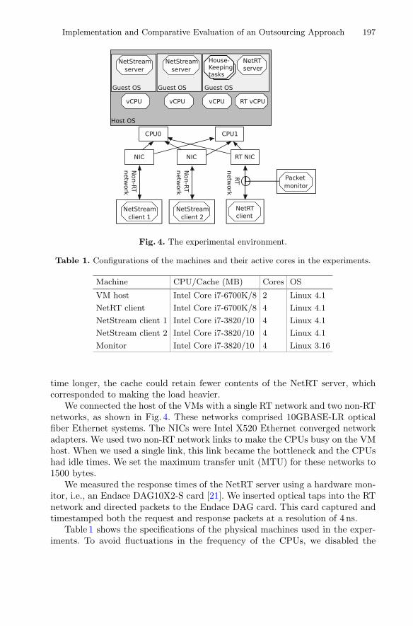
Implementation and Comparative Evaluation of an Outsourcing Approach 197
Fig. 4. The experimental environment.
Table 1. Configurations of the machines and their active cores in the experiments.
Machine CPU/Cache (MB) Cores OS
VM host Intel Core i7-6700K/8 2 Linux 4.1
NetRT client Intel Core i7-6700K/8 4 Linux 4.1
NetStream client 1 Intel Core i7-3820/10 4 Linux 4.1
NetStream client 2 Intel Core i7-3820/10 4 Linux 4.1
Monitor Intel Core i7-3820/10 4 Linux 3.16
time longer, the cache could retain fewer contents of the NetRT server, whichcorresponded to making the load heavier.
We connected the host of the VMs with a single RT network and two non-RTnetworks, as shown in Fig. 4. These networks comprised 10GBASE-LR opticalfiber Ethernet systems. The NICs were Intel X520 Ethernet converged networkadapters. We used two non-RT network links to make the CPUs busy on the VMhost. When we used a single link, this link became the bottleneck and the CPUshad idle times. We set the maximum transfer unit (MTU) for these networks to1500 bytes.
We measured the response times of the NetRT server using a hardware mon-itor, i.e., an Endace DAG10X2-S card [21]. We inserted optical taps into the RTnetwork and directed packets to the Endace DAG card. This card captured andtimestamped both the request and response packets at a resolution of 4 ns.
Table 1 shows the specifications of the physical machines used in the exper-iments. To avoid fluctuations in the frequency of the CPUs, we disabled the

198 O. Garcia et al.
Table 2. NetRT latency comparison between the RT methods (microseconds).
Method Mean 99th percentile Standard deviation
No method (vanilla Linux) 123.0 184.9 22.0
RT Preempt Patch Only 91.8 120.5 11.8
Dedicated processor 58.1 80.8 7.7
Outsourcing 32.6 49.5 2.8
Outsourcing (only RT poll list) 93.2 131.1 11.4
Outsourcing (only RT socket outsourcing) 41.1 64.0 12.2
following processor features: Hyper-threading, TurboBoost and C-States2. Inaddition, we set the CONFIG NO HZ FULL option in both the host and guest ker-nels to reduce the number of clock ticks in the CPU that executed the NetRTserver. For the dedicated processor method, we assigned CPU 0 as the non-RTCPU and CPU 1 as the RT CPU. All guest OSes were Linux 4.1.
4.2 Experimental Results
Figure 5 shows the response times of the NetRT server, and Table 2 shows theirstatistical values (the mean, 99th percentile, and standard deviation (SD)).Figure 6 shows the throughputs and Fig. 7 shows the achievable CPU utiliza-tion.
Figure 5a shows that in vanilla Linux, the NetRT server had high latencyvariance. On the other hand, the execution of NetStream servers presented ahigh performance as shown in Fig. 6, and NetStream servers got a throughputof 18.8 Gbps over an aggregated link capacity of 20 Gbps. The activities of theNetRT server and the NetStream servers did not consume all the CPU resources,as shown in Fig. 7.
Figure 5b shows that the RT Preempt Patch Only method improved thesystem realtimeness compared with vanilla Linux. Despite this improvement,the NetStream servers interfered with the response times of the NetRT server.The CPUs reached their maximum capacities in this method, which limited thevolume of data received by the NetStream servers. Consequently, the NetStreamservers had a throughput of 16.0 Gbps.
Figure 5c shows the response times obtained using the dedicated processormethod. This method reduced the latency variability. However, the dedicatedprocessor method could only use 50% of the CPU resources to execute the Net-Stream servers, which limited the total throughput to 8.6 Gbps.
Figure 5d shows the response times using the outsourcing method that com-prises the two techniques: adding an RT poll list (Sect. 3.1) and RT socket out-sourcing (Sect. 3.2). This method had the lowest latency variability among the
2 C-states are CPU modes for saving power. C-state transitions degrade the perfor-mance of RT services. We disabled C-states in the BIOS and in the Linux kernelusing the parameters intel idle.max cstate=0 and idle=poll.

Implementation and Comparative Evaluation of an Outsourcing Approach 199
Fig. 5. Distribution of the NetRT server response times.
three methods. In addition, the outsourcing method maintained a high through-put of 18.8 Gbps with the lowest CPU consumption.
In summary, compared to the RT Preempt Patch Only method, the out-sourcing method has the 76% lower standard deviation, 15% higher throughput,and 33% lower CPU overhead. Compared to the dedicated processor method,the outsourcing method has the 63% lower standard deviation and higher totalthroughput by a factor of 2, and avoids under-utilization of the dedicated pro-cessor.
We performed the experiment by enabling one of two techniques: adding anRT poll list and RT socket outsourcing. Figure 5e and f show the results. Whenwe enabled only one of the two techniques, we obtained large variability in theresponse times.
4.3 Application Benchmarks
In Sect. 4.2, we compared the three RT methods using netperf as a NetRT server.In this section, we compare these methods using two time-sensitive applicationsas NetRT servers. We used the same experimental environment and configura-tions described in Sect. 4.1.

200 O. Garcia et al.
Fig. 6. Total throughput.
Fig. 7. Achievable CPU utilization.
A Voice over IP Server (VoIP). We measured the forward delays of aVoIP server that used the Session Initiation Protocol (SIP). We measured theimpact of the NetStream servers on the activity of the NetRT server with variousrequesting rates. In this experiment, we ran Kamailio [22], a VoIP server, as theNetRT server. In a remote machine, we ran a SIPp [23] instance as a user agentclient (UAC) and another instance as a user agent server (UAS). The VoIP serverrelayed messages between the UAC and the UAS.
We measured the forward delays between the message the VoIP serverreceived and the message the VoIP server sent in SIP calls. In a single SIPcall, the server forwarded six messages. The UAC first sent an INVITE messageto the server, the server replied with a TRYING message and forwarded theINVITE message to the UAS. Next, the server forwarded a RINGING and OKmessage from the UAS to the UAC. Next, the server forwarded an ACK andBYE message from the UAC to the UAS. Finally, the server forwarded an OKmessage from the UAS to the UAC. We measured these forward delays usingthe hardware monitor, the Endace DAG card. We modified SIPp to make callsat random rates ranging from 17 to 167 calls per second. This means that theserver forwarded 100 to 1000 messages in a second.
Figure 8 shows the 50th, 99th and 99.9th percentiles of the NetRT responsetimes. The response times with the outsourcing method had lower tail latenciesthan those with the RT Preempt Patch Only method and the dedicated processor

Implementation and Comparative Evaluation of an Outsourcing Approach 201
Fig. 8. The forward delays of a voice over IP server (Kamailio).
method. For example, in the 99th percentiles, the outsourcing method had 41%lower latency compared with the RT preempt Patch Only method and 32% lowerlatency compared with the dedicated processor method.
Memcached. We performed another application experiment using Memcached[24] as a NetRT server. Memcached is a distributed caching server that storeskey-value pairs. The NetRT server received requests from a remote client calledmemaslap [25]. We measured the response times using random request intervalsranging from 100 to 1000 requests per second with the hardware monitor, theEndace DAG card. Memaslap sent GET/SET requests at a ratio of 9:1. The sizeof a key was 64 bytes and the size of the value was 1024 bytes. We ran the sameNetStream servers employed in the previous experiments.
Figure 9 presents the 50th, 99th, and 99.9th percentiles of the response times ofthe GET requests. Similar to the previous experiment, the outsourcing methodobtained better results than the RT Preempt Patch Only and the dedicatedprocessor methods. In the 99th percentiles, the outsourcing method had 59%lower latency compared with the RT preempt Patch Only method and 54%lower latency compared with the dedicated processor method.
5 Related Work
The RT Preempt Patch Only and dedicated processor methods [8,15,16,18] areamong the favorite choices in production-use operating systems that support RTservices. Classic proposals for adding real-time support to commodity operatingsystems include RTLinux [26], Time-Sensitive Linux (TSL) [27], and Xenomai[28]. Although these proposed systems have been shown to be effective in reduc-ing latency variance, the results are affected by the continuous evolution of the

202 O. Garcia et al.
Fig. 9. The response times of Memcached.
underlying OS code. Examples of new sources of variance described in Sects. 2.3and 2.5 include priority inversion and cache pollution.
Other proposals to address the priority inversion problem in network process-ing include lazy receiver processing (LRP) [29], which postpones the interrupthandling process until execution of the receiver task, and prioritized interrupthandling [30] for asynchronous transfer mode networks. More generally, someuser space I/O frameworks [31–33] employ a polling mode to avoid latenciescaused by interrupt handling and allow applications to send and receive pack-ets directly from the DMA buffers of a NIC. Other alternatives to improvenetwork throughput include polling threads [31], Data Plane Development Kit(DPDK)/vhostuser [32] and Netmap [33]. These design and implementationalternatives have varied trade-offs in throughput, latency, variance in latency,and achievable CPU utilization, as well as implementation difficulty in commod-ity systems such as Linux and KVM.
The study of software-based methods in this paper complements theadvanced hardware assist techniques to improve I/O performance in VM envi-ronments [10–12,34–36]. Concrete examples include: Exit-Less Interrupts (ELI)[34], Efficient and Scalable Paravirtual I/O System (ELVIS) [35], and DirectInterrupt Delivery (DID) [36], which employ advanced hardware features, suchas Single Root I/O Virtualization (SR-IOV) and Advanced Programmable Inter-rupt Controller virtualization (APICv) by Intel, Advanced Virtual InterruptController (AVIC) by AMD, and Virtual Generic Interrupt Controller (VGIC)by ARM. These new hardware features are able to bypass some of the softwarelayers in a consolidated environment that includes a guest OS, the host OS, andthe VMM. The combination of software techniques such as outsourcing withadvanced hardware assist is another interesting area of future research.
Implementation and Comparative Evaluation of an Outsourcing Approach 203
Previous outsourcing and similar techniques focus on improving throughput[9,37–39]. This is the first paper that uses outsourcing for reducing latency andvariance in latency.
6 Conclusion
In this study, we have proposed the outsourcing method of real-time networkservices in KVM-based commodity hosted environments, and evaluated ourmethod by comparing with two production methods, the RT Preempt PatchOnly method and the dedicated processor method.
First, we found that the RT Preempt Patch Only method is able to reduce andremove the sources of latency variance in interrupt handling, primarily due to thefirst priority inversion problem between RT user processes and non-RT interrupthandling. However, the second priority inversion problem in the softirq mecha-nism of Linux remains. The dedicated processor method dedicates an exclusiveprocessor for RT threads, including softirq, thus removing all thread-related pri-ority inversion problems. Its drawback is that the low utilization of the dedicatedprocessor can significantly reduce the total achievable throughput. The main con-tribution of the paper is the outsourcing method, which is implemented with twomodest modifications to Linux (in addition to the RT Preempt patch). The firstmodification explicitly separates RT softirq handling from non-RT softirq han-dling, removing the second priority inversion problem. The second modificationoutsources the processing of network services from the guest OS to the host OS,thereby mitigating the cache pollution problem and avoiding the second priorityinversion in a guest OS.
Compared to the RT Preempt Patch Only method, the outsourcing methodhas the 76% lower standard deviation, 15% higher throughput, and 33% lowerCPU overhead. Compared to the dedicated processor method, the outsourcingmethod has the 63% lower standard deviation, higher total throughput by afactor of 2, and avoids under-utilization of the dedicated processor.
Acknowledgments. This work was partially supported by JSPS KAKENHI GrantNumber 25540022 and 16K12410.
References
1. Prevot, T.: NextGen technologies for mid-term and far-term air traffic controloperations. In: IEEE/AIAA 28th Digital Avionics Systems Conference, pp. 2.A.4-1–2.A.4-16 (2009)
2. Chen, I.R., Guo, J., Tsai, J.J.P.: Trust as a service for SOA-based IoT systems.Serv. Trans. Internet Things (STIOT) 1(1), 43–52 (2017)
3. Page, A., Hijazi, S., Askan, D., Kantarci, B., Soyata, T.: Support systems for healthmonitoring using Internet-of-Things driven data acquisition. Int. J. Serv. Comput.(IJSC) 4(4), 18–34 (2016)
204 O. Garcia et al.
4. Chang, S.F., Chang, J.C., Lin, K.H., Yu, B., Lee, Y.C., Tsai, S.B., Zhou, J., Wu, C.,Yan, Z.C.: Measuring the service quality of E-Commerce and competitive strate-gies. Int. J. Web Serv. Res. (IJWSR) 11(3), 96–115 (2014)
5. LiDuan, Y., Chen, J.: Event-driven SOA for IoT services. Int. J. Serv. Comput.(IJSC) 2(2), 30–43 (2014)
6. Sun, Y., Qiao, X., Tan, W., Cheng, B., Shi, R., Chen, J.: A low-delay, light-weightpublish/subscribe architecture for delay-sensitive IoT services. Int. J. Web Serv.Res. (IJWSR) 10(3), 60–81 (2013)
7. dmoz.org: List of real-time operating systems. https://dmoztools.net/Computers/Software/Operating Systems/Realtime/. Accessed 1 Nov 2017
8. Rostedt, S., Hart, D.V.: Internals of the RT patch. In: Proceedings of the LinuxSymposium, pp. 161–172 (2007)
9. Eiraku, H., Shinjo, Y., Pu, C., Koh, Y., Kato, K.: Fast networking with socket-outsourcing in hosted virtual machine environments. In: Proceedings of the 2009ACM Symposium on Applied Computing (SAC), pp. 310–317 (2009)
10. Jang, K., Sherry, J., Ballani, H., Moncaster, T.: Silo: predictable message latencyin the cloud. In: Proceedings of the 2015 ACM Conference on Special InterestGroup on Data Communication (SIGCOMM 2015), pp. 435–448 (2015)
11. Chowdhury, M., Liu, Z., Ghodsi, A., Stoica, I.: HUG: multi-resource fairness forcorrelated and elastic demands. In: 13th USENIX Symposium on Networked Sys-tems Design and Implementation (NSDI), pp. 407–424 (2016)
12. Xiong, P., Hacigumus, H., Naughton, J.F.: A software-defined networking basedapproach for performance management of analytical queries on distributed datastores. In: Proceedings of the ACM SIGMOD International Conference on Man-agement of Data, pp. 955–966 (2014)
13. Werner, C., Buschmann, C., Jacker, T., Fischer, S.: Bandwidth and latency con-siderations for efficient SOAP messaging. Int. J. Web Serv. Res. 3(1), 49–67 (2006)
14. KernekShark: KernelShark - a front end reader of trace-cmd (2017). http://rostedt.homelinux.com/kernelshark/. Accessed 27 Oct 2017
15. Red Hat Inc.: Enterprise Linux for Real Time. https://access.redhat.com/documentation/en-US/Red Hat Enterprise Linux for Real Time/7/html/Installation Guide. Accessed 13 May 2017
16. Christofferson, M.: 4 ways to improve performance in embedded Linux systems.Korea Linux Forum (2013)
17. Crespo, A., Ripoll, I., Masmano, M.: Partitioned embedded architecture based onhypervisor: the XtratuM approach. In: Proceedings of the IEEE European Depend-able Computing Conference (EDCC), pp. 67–72 (2010)
18. van Riel, R.: Real-time KVM from the ground up. KVM Forum, August 201519. Jones, R.: Netperf (1996). https://hewlettpackard.github.io/netperf/. Accessed 27
May 201720. Tirumala, A., Qin, F., Dugan, J., Ferguson, J., Gibbs, K.: iPerf: the TCP/UDP
bandwidth measurement tool (2005). http://iperf.sourceforge.net 20 Apr 201721. Endace Technology Limited: DAG10X2-S datasheet (2015). https://www.endace.
com/dag-10x2-s-datasheet.pdf. Accessed 12 June 201722. The Kamailio SIP Server Project: Kamailio SIP server. https://www.kamailio.org/
w/. Accessed 12 May 201723. Gayraud, R., Jacques, O.: SIPp benchmark tool. http://sipp.sourceforge.net/.
Accessed 23 Apr 201724. Memcached: Memcached - a distributed memory object caching system (2015).
https://memcached.org/. Accessed 3 July 2017

Implementation and Comparative Evaluation of an Outsourcing Approach 205
25. Aker, B.: Libmemcached-Memaslap. http://libmemcached.org/libMemcached.html. Accessed 1 Nov 2017
26. Barabanov, M., Yodaiken, V.: Introducing real-time Linux. Linux J. 34 9 p. (1997)27. Goel, A., Abeni, L., Krasic, C., Snow, J., Walpole, J.: Supporting time-sensitive
applications on a commodity OS. In: the USENIX 5th Symposium on OperatingSystems Design and implementation, pp. 165–180 (2002)
28. Gerum, P.: Xenomai - Implementing a RTOS emulation framework onGNU/Linux. http://www.xenomai.org/documentation/xenomai-2.5/pdf/xenomai.pdf. Accessed 4 Nov 2017
29. Druschel, P., Banga, G.: Lazy receiver processing (LRP): a network subsystemarchitecture for server systems. In: the 2nd USENIX Symposium on OperatingSystems Design and Implementation, pp. 261–275 (1996)
30. Kuhns, F., Schmidt, D.C., Levine, D.L.: The design and performance of a real-time I/O subsystem. In: Proceedings of the 5th IEEE Real-Time Technology andApplications Symposium, pp. 154–163 (1999)
31. Liu, J., Abali, B.: Virtualization polling engine (VPE): using dedicated CPU coresto accelerate I/O virtualization. In: The ACM 23rd International Conference onSupercomputing, pp. 225–234 (2009)
32. Intel Corporation: DPDK: Data Plane Development Kit. http://dpdk.org/.Accessed 28 Sept 2017
33. Rizzo, L.: Netmap: a novel framework for fast packet I/O. In: Proceedings of the2012 USENIX Conference on Annual Technical Conference, p. 9 (2012)
34. Gordon, A., Amit, N., Har’El, N., Ben-Yehuda, M., Landau, A., Schuster, A.,Tsafrir, D.: ELI: bare-metal Performance for I/O Virtualization. In: Proceedings ofthe 17th ACM International Conference on Architectural Support for ProgrammingLanguages and Operating Systems, pp. 411–422 (2012)
35. Gordon, A., Har’El, N., Landau, A., Ben-Yehuda, M., Traeger, A.: Towards exitlessand efficient paravirtual I/O. In: Proceedings of the 5th ACM Annual InternationalSystems and Storage Conference (SYSTOR), pp. 1–6 (2012)
36. Tu, C.C., Ferdman, M., Lee, C., Chiueh, T.: A comprehensive implementationand evaluation of direct interrupt delivery. In: Proceedings of the 11th ACMSIGPLAN/SIGOPS International Conference on Virtual Execution Environments(VEE), pp. 1–15 (2015)
37. Gamage, S., Kompella, R.R., Xu, D., Kangarlou, A.: Protocol responsibilityoffloading to improve TCP throughput in virtualized environments. ACM Trans.Comput. Syst. (TOCS) 31(3), 1–34 (2013)
38. Nordal, A., Kvalnes, A., Johansen, D.: Paravirtualizing TCP. In: Proceedings ofthe 6th ACM International Workshop on Virtualization Technologies in DistributedComputing Date (VTDC), pp. 3–10 (2012)
39. Lin, Q., Qi, Z., Wu, J., Dong, Y., Guan, H.: Optimizing virtual machines usinghybrid virtualization. Elsevier J. Syst. Softw. 85(11), 2593–2603 (2012)

Identity and Access Management forCloud Services Used by the Payment
Card Industry
Ruediger Schulze(B)
IBM Germany Research and Development GmbH, Schoenaicher Street 220,71034 Boeblingen, Germany
Abstract. The Payment Card Industry Data Security Standard (PCIDSS) mandates that any entity of the cardholder data environment(CDE) involved in the credit card payment process has to be compli-ant to the requirements of the standard. Hence, cloud services which areused in the CDE have to adhere to the PCI DSS requirements too. Iden-tity and access management (IAM) are essential functions for controllingthe access to the resources of cloud services. The aim of this research is toinvestigate the aspects of IAM required by the PCI DSS and to describecurrent concepts of IAM for cloud services and how they relate to therequirements of the PCI DSS.
1 Introduction
Credit card frauds are committed using different methods. According to [1],60% of the value of fraudulent transactions within the Single Euro PaymentsArea (SEPA) were caused by card-not-present (CNP) payments in 2012. CNPfrauds are committed without the actual physical use of the credit card, e.g. inonline, phone or mail-order transactions. Online merchants are at an increasedrisks due to attacks which target to exploit vulnerabilities and obtain creditcard records for use in CNP frauds and identity theft. The PCI DSS has beenestablished to ensure the safety of the merchant’s payment systems and has to beimplemented by all merchants that provide payment with credit cards. The PCIDSS describes a set of 12 technical and operational requirements in five categoriesto protect credit card data [2]. The importance of the requirements claimed byPCI DSS can be illustrated at the example of the TJX data breach [3]. TheTJX Companies, Inc., a department store chain in the United States, kept themagnetic strip data from customers credit cards in unencrypted from and wasattacked by thieves first time in July 2005. In total, data of 94,000,000 cards wasstolen. The PCI DSS defines some very prescriptive requirements to avoid suchscenarios, e.g. sensitive authentication data must not be stored on storage at alland the primary account number has to rendered in unreadable format whenstored. The requirements of the PCI DSS apply to all entities involved into thepayment process, including service providers. Cloud services involved with creditc© Springer International Publishing AG, part of Springer Nature 2018M. Luo and L.-J. Zhang (Eds.): CLOUD 2018, LNCS 10967, pp. 206–218, 2018.https://doi.org/10.1007/978-3-319-94295-7_14
Identity and Access Management for Cloud Services Used by the PCI 207
card payment have to be PCI DSS compliant. Cloud Service Providers (CSP)which are engaged by merchants as third-part service providers (TPSP) haveto provide evidence of their PCI DSS compliance status [4]. IAM are essentialfunctions when interacting with cloud services. IAM has to ensure that accessto cloud services and related data is only granted to authorized users and thatcompliance with internal policies and external regulations is maintained. Theaim of this research is to examine the IAM related requirements of the PCI DSSand to investigate current methods of IAM in the context of cloud services andPCI DSS. In the following, the requirements of the PCI DSS and the essentialfunctions of IAM for cloud services are described, the PCI DSS requirements areassessed for their relation to the IAM functions and different methods of IAMfor cloud services are analysed.
2 Payment Card Industry Data Security Standard
The PCI DSS has been issued to ensure the security of credit card and accountdata [2]. The latest version 3.2 of the standard has been released in April 2016[2]. The technical and operational requirements of the PCI DSS apply to allentities involved in the process of the credit card payment. The scope of thePCI DSS is extensive. Any component included in the CDE is to be considered,including people, processes and technologies. The entities to be compliant withPCI DSS include merchants, processors, acquirers, issuers and services providersbut also any entities that store, process or transmit cardholder data and sensitiveauthentication data. PCI DSS defines 12 requirements and corresponding testprocedures which are combined into a security assessment tool for use duringPCI DSS compliance assessments. The following requirements are to be assessedusing the test procedures in the validation process [2]:
2.1 Build and Maintain a Secure Network and Systems
1. Install and maintain a firewall configuration to protect cardholder dataFirewalls control the traffic between an entity’s internal network and theuntrusted, external networks, and the traffic in and out of sensitive areaswithin the internal trusted network. Firewalls and router configurations haveto be established and implemented following a formal process for approvingand testing all network connections and using documentation of businessjustification and network diagrams.
2. Do not use vendor-supplied defaults for system passwords and other securityparametersIntruders (external and internal) use default passwords or exploits basedon default system settings to compromise systems. The information aboutdefault passwords and settings are widely known and can easily be obtainedfrom public documentation. Vendor-supplied defaults must always be changedand unnecessary default accounts be removed before a system is connectedto the network.

208 R. Schulze
2.2 Protect Cardholder Data
3. Protect stored cardholder dataCardholder data refers to any information present in any form on a paymentcard. The cardholder data must be protected by the entities accepting pay-ment cards and unauthorized use has to be prevented. Methods like encryp-tion, cutting, masking and hashing have to be used in order to transfer andprocess the data in an unreadable form. Only limited cardholder data shouldbe stored on storage. Sensitive authentication data must not be stored afterauthentication.
4. Encrypt transmission of cardholder data across open, public networksIntruders exploit the misconfiguration of wireless network devices and weak-nesses in legacy encryption and authentication protocols to gain access toCDE. Strong encryption and security protocols must be used to protect thecardholder data during transmission over open and public networks.
2.3 Maintain a Vulnerability Management Program
5. Protect all system against malware and regularly update anti-virus softwareor programsMalicious software (malware) such as viruses, worms and trojans can enterthe network during approved business activities, e.g. via employee e-mail andthe use of the Internet, and target to exploit system vulnerabilities. Anti-virussoftware has to be installed on all systems potentially affected by malicioussoftware. The anti-virus software has to be capable to detect, remove andprotect against all types of malicious software. It has to be ensured that theanti-virus mechanisms can not be disabled and are kept current, i.e. virussignature files are regularly updated and scans are executed.
6. Develop and maintain secure systems and applicationsIntrudes use security vulnerabilities to gain privileged access to the systems.Many of these vulnerabilities can be fixed by security patches provided bythe vendors. Therefore, a process has to be established to regularly identifysecurity vulnerabilities, rank them by risk (e.g. “high”, “medium”, “low”)and install applicable vendor-supplied security patches. Critical patches mustbe installed within a month after release.
2.4 Implement Strong Access Control Measures
7. Restrict access to cardholder data by business need to knowThe access to cardholder data must be limited to authorized personnel. Sys-tems and processes have to be in place to control and restrict the access tothe cardholder data. Access must only be granted on the base of businessneeds and in accordance with the job responsibility.
8. Identify and authenticate access to system componentsAn unique identification (ID) has to be assigned to each person with access to

Identity and Access Management for Cloud Services Used by the PCI 209
the CDE. Personalized IDs ensure that each individual can be held account-able for their actions. Using IDs, activities performed on critical data andsystems can be restricted to authorized users only and be traced for auditing.An authentication system must be in place which implements the policies foradding, deleting and modifying user IDs and credentials. The authenticationsystem has to effectively enforce protection, e.g. by limiting the number ofaccess attempts and requesting regular password changes.
9. Restrict physical access to cardholder data by business need to knowPhysical access to systems that host cardholder data must be restricted toavoid unauthorised access to devices or data, and prevent removal or deletionof devices or hard-copies. Appropriate facility entry controls must be in placeto limit and monitor the physical access to the systems of the CDE.
2.5 Regularly Monitor and Test Networks
10. Track and monitor all access to network resources and cardholder dataAll access to the cardholder data must be tracked and monitored. Loggingmechanisms and tracking of user activities enable effective forensics and vul-nerability management. The existence of logs in all environments allows forthorough tracking, warning and analysis in the event of a fault. Audit trailshave to be implemented that link all access to the system to an individualuser and allow to reconstruct events such the user access to the cardholderdata and invalid access attempts. Regular reviews of logs and security eventshave to be established to identify anomalies and suspicious activities.
11. Regularly test security system and processesVulnerabilities are continually discovered by both intruders and researchers.New vulnerabilities are often introduced by new software. System compo-nents, processes and custom software have to be tested regularly to ensurethat security is maintained over time. Tests have to include the verificationof the security controls for wireless access points, vulnerability scans of theinternal and external network, penetration tests, intrusion detection andchange detection for unauthorized modification.
2.6 Maintain an Information Security Policy
12. Maintain a policy that addresses information security for all personnelAll personnel have to understand the sensitivity of the data and their respon-sibility to protect it. Strong security policies have to be enforced for theentire entity of the CDE and inform all personnel what is expected of them.
In [5], the fact that the PCI DSS 3.0 implies many changes compared tothe version 2.0 is investigated. Even organisations which are already PCI DSS2.0 compliant may encounter challenges when moving to the new version. Thechanges between PCI DSS 2.0 and 3.0 are identified and PCI DSS 3.0 is imple-mented at the example of the largest company for online payment services inIndonesia to measure an organisation’s compliance level. As a result of this

210 R. Schulze
research 182 new controls are identified which simplify the adoption of PCI DSS3.0 by an organisation that is already compliant to the PCI DSS 2.0. The com-pany was found to be 77.43% compliant to the PCI DSS 3.0 requirements. One ofthe recommendations in [5] is that the company should implement strict accesscontrols to limit the access to card holder data as per PCI DSS requirement 7.The PCI Compliance Report from 2015 [6] shows that victims of data breachesstruggle with establishing restricted access and access authentication more thanother organisations. The report positively points out that the compliance withrequirement 7 increased over the last year to 89% of all investigated companiesin 2014. The compliance with requirement 8 for access authentication was at69% in 2014. Some companies still have challenges with establishing appropriatehandling of credentials (8.2) and preventing shared use of credentials (8.5).
3 Identity and Access Management for Cloud Services
With the adoption of cloud services, functions of the IAM have to be extendedinto the CSP. The following IAM functions are essential for the successful andeffective management of identities when using cloud services [7]:
1. Identity Provisioning and User ManagementThe existing processes for user management within an enterprise have to beextended to cloud services. Identity provisioning has to handle the secureand timely management of on-boarding and off-boarding the users of cloudservices. The users of the cloud services represent either individuals or theorganisation and are maintained by the CSP in order to support authentica-tion, authorisation, federation, billing and auditing processes. The provision-ing of the users for a specific cloud service has to be done with appropriateprivileges and based on their roles as cloud service consumer, e.g. businessmanager, administrator, service integrator and end user. CSP have to provideAPIs which support the provisioning of users and consumer organisations mayuse automated identity management solutions exploiting those APIs.
2. Authentication and Credential ManagementAuthentication validates the credentials provided by a user. Organisationsthat become cloud service consumers have to invest into properly handlingcredential management, strong authentication and delegated authentication,and how trust is managed across multiple cloud services. Credential manage-ment involves the processes for managing passwords, digital certificates anddynamic credentials. One time passwords and strong authentication such asmulti-factor authentication should be used to reduce for instance the impactof compromised password. Credentials may be stolen by various types of intru-sion attempts such as phishing, key-logging or man-in-the-middle attacks. Theimpact of stolen credentials is fatal, data can be monitored or manipulated,and compromised valid user accounts can be used for denial-of-service attacksor obtaining root level access to VMs and hosts [8].
Identity and Access Management for Cloud Services Used by the PCI 211
3. FederationFederation enables cloud service consumers to authenticate as users of cloudservices using their chosen identity provider. The identity provider is anauthoritative source which provides authentication of the users. The federa-tion process requires that identity attributes are securely exchanged betweena service provider and the identity provider. The service provider can be eitheran internally deployed application or a cloud service. Multiple federation stan-dards exist today. The Security Assertion Markup Language (SAML) is awidely accepted federation standard and supports single sign-on (SSO). Asorganisations start to consume multiple cloud services, SSO becomes impor-tant in order to manage authentication across these different services consis-tently using a central identity provider.
4. Authorisation and User Profile ManagementAuthorisation grants access to requested resources based on user profileattributes and access policies. The user profile stores a set of attributes whichthe CSP uses to customize the service and to restrict or enable access to sub-sets of functions of the service. For users which act on behalf of an organisa-tion, some of the user’s profile attributes, e.g. the user role, may be assignedby the organisation. The organisation is in this case the authoritative sourcefor those attributes and owns the access control policy to be applied to theusers. Organisations have to manage the profile attributes for their users ofcloud service and have to confirm with the CSP based on their requirementsthat adequate access control mechanisms of the cloud resources are supported.
5. ComplianceCloud service consumers have to understand how CSPs enable compliancewith internal and external regulatory requirements. When consuming cloudservices, some of the information required to satisfy audit and compliancereporting requirements has to be delivered by the CSP.
The classification of different Identity Management Systems (IDMS) for cloudservices are discussed in [9–11]:
1. Isolated IDMSA single server is used as service provider and identity provider. The systemdoes not rely on a trusted third party for credential issuance and verifica-tion. User accounts are replicated from the on-premise user directory into thecloud environment. Using this approach introduces security exposures whensensitive data like passwords or keys are exposed into the cloud. Changes toroles and user ID removal become effective delayed as the replication occursasynchronous.
2. Centralised IDMSThe service provider(s) and the identity provider run on different servers. Onededicated server is used as identity provider for issuing and managing useridentities, while any other servers are responsible for providing cloud services.
212 R. Schulze
3. Federated IDMSFederation allows to manage user identities within an organisation using anon-premise user directory. Users of federated IDMS can use the same creden-tials for authenticating to different cloud services. User identities are validatedusing tokens issued by the identity provider and presented to the cloud serviceinterface. A cloud-based form of federated IDMS are Identity Management-as-a-Service (IDMaaS) systems. In this case, a separate cloud service managesthe identity, provides identity federation with other cloud services and allowsan identity to be linked with multiple cloud services.
4. Anonymous IDMSThe user’s identity management information is not disclosed to others duringauthentication and the user is kept anonymous.
4 PCI DSS Requirements for Identity and AccessManagement
The PCI DSS requirements impose a set of requirements related to IAM, inparticular the requirements for strong access control are related to the IAMfunctions [2]. In [12], an approach for migrating PCI DSS compliance to anInfrastructure-as-a-Service (IaaS) provider is described. The article emphasisesthe shared responsibility of organisations and CSPs for ensuring PCI DSS com-pliance for the IAM related requirements. Typically, IaaS providers enable PCIDSS compliance at the physical infrastructure level, and support multi-factorauthentication and role-based policies, while the users of the organisations haveto perform the IaaS account management.
4.1 Identity Provisioning and User Management
PCI DSS requirement 8 formulates the detailed requirements for managing iden-tity within the CDE1 [2]:
1. All users of the CDE must receive a unique ID before allowing them to accesscomponents of the CDE or cardholder data (8.1.1).
2. Strong processes for managing the life cycle of the user IDs must be in place.User accounts must be valid and be associated with a person currently presentin the organisation. Changes such as adding new user IDs, modifying or delet-ing existing ones must be performed under the control of these processes(8.1.2).
3. User IDs of terminated users must be revoked immediately (8.1.3).4. User accounts which are not used within the last 90 days have to be removed
or disabled (8.1.4).5. User IDs of external vendors should only be enabled during the time period
when needed and be disabled when not in use. Timely unlimited access tothe CDE by vendors increases the risk of unauthorised access. The use of theuser IDs has to be monitored (8.1.5).
1 The numbers in parenthesis refer to the specific PCI DSS requirements.

Identity and Access Management for Cloud Services Used by the PCI 213
6. Security policies and operations procedures for identification must be docu-mented, in use and known to all affected parties (8.8).
4.2 Authentication and Credential Management
PCI DSS requirement 8 demands the implementation of the following authen-tication and credential management related features by the IAM system of thecloud services [2]:
1. Authentication to the CDE must be done by using the user ID and at leastone of methods (8.2):
(a) Something you know (password, passphrase)(b) Something you have (smart card, token device)(c) Something you are (biometric)
2. Two-factor authentication must be used when accessing the CDE fromremote networks. Two of the three authentication methods above have tobe used for authentication (8.3).
3. Strong processes to control the modification of credentials have to be estab-lished (8.1.2).
4. The number of attempts to use invalid credentials for an user IDs has to belimited. After not more than six attempts the user ID has to be locked out(8.1.6).
5. Once an user ID is locked out due to too many attempts with invalid creden-tials, the lockout duration has to be at least 30 min or until an administratorenables the user ID again (8.1.7).
6. Re-authentication is required after a session is idle for more than 15 min(8.1.8).
7. All credentials must be rendered unreadable using strong cryptography dur-ing transmission and when stored on storage (8.2.1).
8. Before the modification of any authentication credentials, the identity of theusers has to be verified (8.2.2).
9. Passwords and passphrases must have a minimum length of at least sevencharacters and contain both numeric and alphabetic characters (8.2.3)
10. Passwords and passphrases must be changed at least every 90 days (8.2.4).11. When a user changes the credentials of its user ID, it must to be ensured
that the new password or passphrases is not the same for any of the lastfour passwords or passphrases used before (8.2.5).
12. Passwords and passphrases for first-time use or upon reset have to be uniquefor each user and must be changed immediately after the first login (8.2.6).
13. Group, shared or generic IDs and passwords must not be used for authenti-cation (8.5).
14. Authentication policies and procedures must be documented and communi-cated (8.4).
15. Security policies and operation procedures for authentication must be doc-umented, in use and known to all affected parties (8.8).

214 R. Schulze
4.3 Federation
The PCI DSS does not give any explicit requirements related to federation. Theidentity provider for authenticating users when working with federation belongsto the CDE. In case of cloud services which are used as identity provider, theprovider of the services is to be treated as TPSP from the perspective of theCDE and the requirements of the PCI DSS apply to it.
4.4 Authorisation
The authorisation functions of the cloud IAM have to support the followingrequirements of the PCI DSS [2]:
1. Access to the components of the CDE and cardholder data must to be limitedto users whose job requires such access (7.1).
2. Based on the job responsibilities and functions, access needs and requiredprivileges have to be defined for each user role (7.1.1).
3. The access of privileged user IDs must be restricted to the least privilegesnecessary to perform a job responsibility (7.1.2).
4. Access must only be assigned based on the user’s individual job classificationand function (7.1.3).
5. Privileges must be assigned to users according to their job classification andfunction, and only after documented approval (7.2.2, 8.1.1).
6. The access control system must be set to “deny all” for all components ofthe CDE and only grant access to users with the need to know as per theirassigned role and privileges (7.2, 7.2.1, 7.2.3).
7. Direct access to the databases containing cardholder data is restricted toonly database administrators. All other access to the database is throughprogrammatic methods using dedicated application IDs. Application IDs arerestricted for only the use by applications (8.7).
8. Security policies and operation procedures for restricting access to cardholderdata must be documented, in use and known to all affected parties (7.3).
4.5 Compliance
In order for cloud services to be conform with the PCI DSS, the following mech-anisms for tracking user activities using audit logs have to be established [2]:
1. All user access to cardholder data must be logged (10.2.1).2. All actions taken by an user with root or administrative privileges must be
logged (10.2.2).3. All access to audit logs must be logged (10.2.3).4. All invalid access attempts must be logged (10.2.4).5. All activities of user management and elevation of privileges must be logged
(10.2.5).6. The initialization, stopping or pausing of the audit logs must be logged
(10.2.6).

Identity and Access Management for Cloud Services Used by the PCI 215
7. Creation and deletion of system-level objects must be logged (10.2.7).8. User identification, type of event, date and time, success or failure identi-
fication, origination of the event and identification or name of the affecteddata, system component or resources must be logged at least for each of theabove events (10.3).
9. Time-synchronization of all clocks must be implemented to ensure eventscaptured in different logs can be correlated (10.4).
10. Audit logs must be secured so that they can not be altered (10.5).11. Audit logs must be reviewed regularly, and in particular all security events
and logs of critical components daily (10.6.).12. Audit logs must be retained at least one year, with a minimum of three
month to be available immediately (10.7).13. Security policies and operation procedures for monitoring all access to net-
work resources and cardholder data must be documented, in use and knownto all affected parties (10.8).
5 IAM Methods for Cloud Services
Methods for cloud IAM are investigated by multiple authors. In [13], a modelfor identity and trust management in cloud environments is proposed. In thismodel, both CSP and users have to register to a trusted authority and obtaina certificate access token. By validating the user’s certificate, the CSP can besure that the user’s request comes from an authentic source. A high performanceIAM system on the base of OpenStack Keystone is proposed in [14]. An intrusiontolerant identity provider is described in [15] and an approach for federation andSSO on the base of claim-based identity management is discussed in [16].
Strong user authentication is a requirement of the PCI DSS. The methodspublished in [17,18] are described below in detail. In [17], a method is proposedwhich combines different security features such as identity management, mutualauthentication and session key agreement between users. Based on two-factorauthentication and two different communication channels, the following authen-tication flow is described:
1. A smart card is issued to the user. The data on the smart card is encryptedusing secret numbers for both the user and server.
2. The user logs into a terminal using a smart card, user ID and password.The authenticity of the user is verified based on the smart card, user ID andpassword.
3. The user sends from the terminal a login request to the cloud server.4. The cloud server generates a one-time key and calculates some hash string.5. The cloud server sends back the hash string to the terminal.6. The cloud server sends the one-time key to the mobile phone of the user via
SMS.7. The user enters the one-time key into the terminal and the key is validated
based on the hash string and data on the smart card.

216 R. Schulze
8. An authentication request is sent to the cloud server using the data of thesmart card, the user ID and the one-time key.
9. The cloud server checks if the maximum legal time of an authenticationsession is not yet passed.
10. The cloud server calculates the validation data based the authenticationrequest and verifies the user’s identity.
11. The cloud server authenticates the user by calculating a session key whichis sent as a hash string back to the user’s terminal.
Methods with communication via two channels and authentication using addi-tional one-time keys are already used by some financial institutes today. Theproposed method enhances these existing mechanisms by combining them withadditional flows for user and server authentication and secure encoding of mes-sages. The method fulfils the PCI DSS requirement 8.3 to use two-factor authen-tication when interacting with cloud services within the CDE from remote net-works. In order to use the method in a PCI DSS compliant environment, theother requirements for authentication and managing credentials must be satis-fied as well. The methods assumes that the user’s password is only stored onsmart card. In this case, the terminal software would have to ensure that therequirements for password such as minimum length and difference from previouspasswords are ensured.
Another method focusing on strong user authentication is proposed in [18].The suggested model uses virtual device authorisation (VDA) and adds anauthentication agent to the user’s web browser. VDA is a Software-as-a-Service(SaaS) application that acts as an gateway to other cloud services. The VDAis used to identify the ownership of private devices and to establish the linkagebetween the clients and the cloud services. A cloud service user may register mul-tiple devices in the VDA for either temporary or permanent authentication tocommunicate with a cloud service. During the registration of a device, approvalis obtained that the device is allowed to access the cloud service and the uniqueaccess code of the authentication agent is generated by the VDA using the device’sMAC address, the access type (permanent or temporary) and an user-providedpasscode. The authentication agent is sent to the client and installed into theuser’s web browser. When the user makes a request to a cloud service, the authen-tication agents confirms the identity of the user based on the passcode. Once theVDA receives confirmation about the identity of the user, the VDA validates theauthorisation of the device. With the proposed method, a CSP can restrict theaccess to cloud services for only approved devices and users. The method leaves itopen to establish further mechanisms for user authentication for each of the cloudservices. The method implements a form of two-factor authentication (1. some-thing you have - an uniquely identified and approved device and 2. something youknow - the user’s passcode) and addresses therefore requirement 8.3 of the PCIDSS. As with the other authentication method described previously, it is neces-sary to also establish mechanisms to satisfy the other PCI DSS requirements forauthentication and credential management. For instance, a re-registration of each
Identity and Access Management for Cloud Services Used by the PCI 217
device will be required at least every 90 days, as the passcode is used for generatingthe unique code of the authentication agent.
6 Conclusions
In this article, the PCI DSS was analysed for the IAM specific requirementsand how they are related to the use of cloud services. Two existing methodsfor authenticating cloud services were analysed. Both methods fulfill the PCIDSS requirement 8.3 for two-factor authentication. With respect to the IAMrelated requirements of the PCI DSS, it was found that current research primarilyfocuses on the requirements for strong authentication. Further research needsto be done for establishing effective methods that address the other PCI DSSrequirements for IAM in cloud environments.
References
1. Third report on card fraud, European Central Bank, February 2014. https://www.ecb.europa.eu/pub/pdf/other/cardfraudreport201402en.pdf
2. Payment Card Industry (PCI) Data Security Standard Version 3.2, April 2016.https://www.pcisecuritystandards.org/documents/PCI DSS v3-2.pdf
3. Shaw, A.: Data breach: from notification to prevention using PCI DSS. Colum. JLSoc. Probs. 43, 517 (2009)
4. PCI Data Security Standard (PCI DSS) 3.0 Information Supplement: Third-Party Security Assurance, August 2014. https://www.pcisecuritystandards.org/documents/PCI DSS V3.0 Third Party Security Assurance.pdf
5. Shihab, M., Misdianti, F.: Moving towards PCI DSS 3.0 compliance: a case studyof credit card data security audit in an online payment company. In: 2014 Inter-national Conference on Advanced Computer Science and Information Systems(ICACSIS), pp. 151–156, October 2014
6. PCI Compliance Report, Verizon 2015. http://www.verizonenterprise.com/pcireport/2015/
7. Kumaraswamy, S., Lakshminarayanan, S., Stein, M.R.J., Wilson, Y.: Domain 12:guidance for identity & access management v2.1. Cloud Secur. Alliance (CSA), 10(2010)
8. Fernandes, D.A., Soares, L.F., Gomes, J.V., Freire, M.M., Inacio, P.R.: Securityissues in cloud environments: a survey. Int. J. Inf. Secur. 13(2), 113–170 (2014)
9. Habiba, U., Abassi, A., Masood, R., Shibli, M.: Assessment criteria for cloud iden-tity management systems. In: 2013 IEEE 19th Pacific Rim International Sympo-sium on Dependable Computing (PRDC), pp. 188–195, December 2013
10. Ma, X.: Managing identities in cloud computing environments. In: 2015 2nd Inter-national Conference on Information Science and Control Engineering (ICISCE),pp. 290–292, April 2015
11. Understanding and Selecting Identity and Access Management for CloudServices, Securosis, June 2013. https://securosis.com/assets/library/reports/Understanding IAM For Cloud Full.pdf
12. Ensuring PCI DSS Compliance in the Cloud, Cognizant (2014). http://www.cognizant.com/InsightsWhitepapers/Ensuring-PCI-DSS-Compliance-in-the-Cloud-codex879.pdf
218 R. Schulze
13. Nida, Teli, B.: An efficient and secure means for identity and trust managementin cloud. In: 2015 International Conference on Advances in Computer Engineeringand Applications (ICACEA), pp. 677–682, March 2015
14. Faraji, M., Kang, J.-M., Bannazadeh, H., Leon-Garcia, A.: Identity access man-agement for multi-tier cloud infrastructures. In: 2014 IEEE Network Operationsand Management Symposium (NOMS), pp. 1–9, May 2014
15. Barreto, L., Siqueira, F., Fraga, J., Feitosa, E.: An intrusion tolerant identity man-agement infrastructure for cloud computing services, In: 2013 IEEE 20th Interna-tional Conference on Web Services (ICWS), pp. 155–162, June 2013
16. Singh, A., Chatterjee, K.: Identity management in cloud computing through claim-based solution. In: 2015 Fifth International Conference on Advanced ComputingCommunication Technologies (ACCT), pp. 524–529, February 2015
17. Choudhury, A., Kumar, P., Sain, M., Lim, H., Jae-Lee, H.: A strong user authenti-cation framework for cloud computing. In: 2011 IEEE Asia-Pacific Services Com-puting Conference (APSCC), pp. 110–115, December 2011
18. Fatemi Moghaddam, F., Khanezaei, N., Manavi, S., Eslami, M., Samar, A.: UAA:user authentication agent for managing user identities in cloud computing envi-ronments. In: 2014 IEEE 5th Control and System Graduate Research Colloquium(ICSGRC), pp. 208–212, August 2014
Network Anomaly Detectionand Identification Based on Deep
Learning Methods
Mingyi Zhu, Kejiang Ye(B), and Cheng-Zhong Xu
Shenzhen Institutes of Advanced Technology, Chinese Academy of Sciences,Shenzhen, China
{my.zhu,kj.ye,cz.xu}@siat.ac.cn
Abstract. Network anomaly detection is the process of determiningwhen network behavior has deviated from the normal behavior. Thedetection of abnormal events in large dynamic network has becomeincreasingly important as networks grow in size and complexity. How-ever, fast and accurate network anomaly detection is very challenging.Deep learning is a potential method for network anomaly detection due toits good feature modeling capability. This paper presents a new anomalydetection method based on deep learning models, specifically the feed-forward neural network (FNN) model and convolutional neural network(CNN) model. The performance of the models is evaluated by severalexperiments with a popular NSL-KDD dataset. From the experimentalresults, we find the FNN and CNN models not only have a strong mod-eling ability for network anomaly detection, but also have high accuracy.Compared with several traditional machine learning methods, such asJ48, Naive Bayes, NB Tree, Random Forest, Random Tree and SVM,the proposed models obtain a higher accuracy and detection rate withlower false positive rate. The deep learning models can effectively improveboth the detection accuracy and the ability to identify anomaly types.
1 Introduction
In today’s large-scale computer networks, an immense amount of flow data areobserved each day, among which there are some records that do not conformto the normal network behavior. Some of them are malicious and can causeserious damage to the network. Therefore, it is important to sift through trafficdata and detect anomalous events as they occur to ensure timely correctiveactions. Network anomalies stand for a large fraction of the Internet traffic andcompromise the performance of the network resources [1]. Possible reasons fortraffic anomalies are changes in the network topology (e.g., newly connectedhosts, routing changes) or network usage (e.g., changed customer behavior, newapplications). Anomalies may also be caused by failures of network devices aswell as by malicious worm or attack traffic [2]. The early detection of such eventsis of particular interest as they may impair the safe and reliable operation of thenetwork.c© Springer International Publishing AG, part of Springer Nature 2018M. Luo and L.-J. Zhang (Eds.): CLOUD 2018, LNCS 10967, pp. 219–234, 2018.https://doi.org/10.1007/978-3-319-94295-7_15
220 M. Zhu et al.
Network anomaly detection aims to detect patterns in a given network trafficdata that do not conform to an established normal behavior [3] and has becomean important area for both commercial interests as well as academic research.Applications of anomaly detection typically stem from the perspectives of net-work monitoring and network security. In network monitoring, a service provideris often interested in capturing such network characteristics as heavy flows thatuse a link with a given capacity, flow size distributions, and the number ofdistinct flows. In network security, the interest lies in characterizing known orunknown anomalous patterns of an attack or a virus. The anomalies may wastenetwork resources, cause performance degradation of network devices and endhosts, and lead to security issues concerning all Internet users. Although networkanomaly detection has been widely studied, it remains a challenging task due tothe following factors:
– In large and complicated networks, the normal behavior can be multi-modal,and the boundary between normal and anomalous events is often not precise.
– Usually the network attacks adapt themselves continuously to cheat the fire-walls and security filters, making the anomaly detection problem more diffi-cult.
– Network traffic data often contains noise which tends to be similar to the trueanomalies, and it is difficult to remove them.
In recent years, deep learning has grown very fast and achieved good resultsin many scenarios. There is a trend to use deep learning technologies for anomalydetection [4]. These feature learning approaches and models have been successfulto a certain extent and match or exceed state of the art techniques.
This paper presents an anomaly detection method using deep learning mod-els, specifically the feedforward neural network (FNN) model and convolutionalneural network (CNN) model. The performance of the model is evaluated byseveral experiments with a popular NSL-KDD dataset [5]. From the experimen-tal results, we find the FNN and CNN models not only have a strong modelingability for network anomaly detection, but also have high accuracy. Comparedwith several traditional machine learning methods, such as J48, Naive Bayes,NB Tree, Random Forest, Random Tree and SVM, the proposed models obtaina higher accuracy and detection rate with lower false positive rate. The deeplearning models can effectively improve both the detection accuracy and theability to identify anomaly types.
2 The Models
2.1 Feedforward Neural Networks
Feedforward neural networks (FNN) are called networks because they are typ-ically represented by composing together many different functions. The modelis associated with a graph describing how the functions are composed together.For example, we might have three functions f (1), f (2), and f (3) connected in a

Network Anomaly Detection and Identification 221
chain, to form f(x) = f (3)(f (2)(f (1)(x))). These chain structures are the mostcommonly used structures of neural networks. In this case, f (1) is called the firstlayer of the network, f (2) is called the second layer, and so on. The overall lengthof the chain gives the depth of the model. It is from this terminology that thename deep learning arises. The final layer of a feedforward network is called theoutput layer.
During neural network training, we drive f(x) to match f∗(x) to get ourmodel. The training data provides us with noisy, approximate examples of f∗(x)evaluated at different training points. Each example x is accompanied by a labely ≈ f∗(x). The training examples specify directly what the output layer like ateach point x; it must produce a value that is close to y. The behavior of otherlayers is not determined by the training data. The learning algorithm must decidehow to use these layers to produce the desired output, but the training datadoes not show what each individual layer does. Instead, the learning algorithmmust know how to use these layers to achieve best implementation. Because thetraining data does not show the output for each of these layers, so that they arecalled hidden layers.
2.2 Convolutional Neural Network
A CNN (Convolutional Neural Network) consists of an input and an output layer,as well as multiple hidden layers, see Fig. 1 as an example. The hidden layers ofa CNN typically consist of convolutional layers, pooling layers, fully connectedlayers and normalization layers. Description of the process as a convolution inneural networks is by convention. Mathematically it is a cross-correlation ratherthan a convolution.
Fig. 1. Convolutional Neural Network
Convolutional. Convolutional layers apply a convolution operation to theinput data, passing the result to the next layer. The convolution emulates theresponse of an individual neuron to stimulation. Each convolutional processesdata only when it just in its responsed field. Although fully connected feedfor-ward neural networks can be used to learn features to classify data, a very highnumber of neurons would be necessary, when we design a deep architecture. The

222 M. Zhu et al.
convolution operation brings a solution to this problem as it reduces the numberof free parameters, allowing the network to be deeper with fewer parameters.In this way, it resolves the vanishing or exploding gradients problem in trainingtraditional multi-layer neural networks with many layers by using backpropaga-tion.
Pooling. Convolutional networks may include local or global pooling layers,which combine the outputs of neuron clusters at one layer into a single neuronin the next layer. Usually, we use the average output of these neurons as a result.
Fully Connected. Fully connected layers connect every neuron in one layerto every neuron in another layer. It is in principle the same as the traditionalmulti-layer perceptron neural network (MLP).
Weights. CNNs share weights in convolutional layers, which means that thesame filter is used for each receptive field in one layer repeatedly, this can reducesmemory use and improves performance.
3 The Proposed Methods
3.1 The Dataset
We used NSL-KDD dataset [5] in our work. NSL-KDD is a dataset suggestedto solve some of the inherent problems of the KDD’99 dataset. The KDD Cupincludes normal and different kinds of attack traffic, such as DoS, Probing, user-to-root (U2R), and root-to-local (R2L). The network traffic for training wascollected for seven weeks. The KDD Cup dataset has been widely used as abenchmark dataset for many years in the evaluation of NIDS (Network Intru-sion Detection Systems) before. However, one of the major drawback with thedataset is that it contains an enormous amount of redundant records both in thetraining and testing data. It was observed that almost 78% and 75% records areredundant in the training and test dataset, respectively. This redundancy makesthe learning algorithms more sensitive towards the frequent attack records andleads to poor classification results for the infrequent, but harmful records.
NSL-KDD was proposed to overcome the limitation of KDD Cup dataset.The dataset is derived from the KDD Cup dataset. It improved the previousdataset in four ways. First, It does not include redundant records in the trainingset, so the classifiers will not be biased towards more frequent records. Second,There is no duplicate records in the proposed testing sets; therefore, the perfor-mance of the learners are not biased by the methods which have better detectionrates on the frequent records. Further, The number of selected records from eachdifficulty level group is inversely proportional to the percentage of records in theoriginal KDD dataset. As a result, the classification rates of distinct machinelearning methods vary in a wider range, which makes it more efficient to have

Network Anomaly Detection and Identification 223
an accurate evaluation of different learning techniques. Moreover, the number ofrecords in the training and testing sets are reasonable, which makes it affordableto run the experiments on the complete set without the need to randomly selecta small portion. Consequently, evaluation results of different research works willbe consistent and comparable.
This dataset contains a training set, KDDTrain+ and two testing sets calledKDDTest+ and KDDTest21. KDDTrain+ includes the full NSL-KDD trainingset with attack-type labels in CSV format and KDDTest+ includes the fullNSL-KDD testing set with attack-type labels in CSV format. In addition, thedataset providers analyzed the difficulty level of the records in KDD dataset.Surprisingly, about 98% of the records in the training set and 86% of the recordsin the testing set were correctly classified with 21 learners. So, they deletedthe examples which are detected by all 21 learners from KDDTest+ and formanother testing set - KDDTest21.
Each record in the NSL-KDD dataset consists of 41 features mentioned inTable 1 and is labeled with either normal or a particular kind of attack. Thesefeatures include basic features derived directly from a TCP/IP connection, trafficfeatures accumulated in a window interval, either time, e.g. two seconds, orseveral connections, and content features extracted from the application layerdata of connections, that shows in Table 1. Among 41 features, three are nominal,four are binary, and remaining 34 are continuous. The training data contains 23traffic classes that include 22 classes of attack and one normal class. The testingdata contains of 38 traffic classes that include 21 attack classes from the trainingdata, 16 novel attacks, and one normal class.
The NSL-KDD also has five categories: Normal, DoS, Probe, user-to-root(U2R), and root-to-local (R2L). Table 2 shows the sample number for the fivecategories. There are totally 125973 samples in training set with 67343 Normalsamples, 45927 DoS samples, 995 R2L samples, 52 U2R samples and 11656 Probesamples. As well as in testing set, there are 22544 samples in all, including 9711Normal samples, 7458 DoS samples, 2754 R2L samples, 200 U2R samples and2421 Probe samples.
3.2 Data Preprocessing
Numericalization. There are 38 numeric features and 3 non-numeric featuresin the NSL-KDD dataset. Because the input value of our models should bea numeric matrix, we must convert some non-numeric features, such as ‘proto-col type’, ‘service’ and ‘flag’ features, into numeric form. For instance, the feature‘protocol type’ has three kinds of attributes, which are ‘tcp’, ‘udp’, and ‘icmp’.And then we encode these values into binary vector (1,0,0), (0,1,0) and (0,0,1).Similarly, the feature service has 70 kinds of attributes, and the feature ‘flag’ has11 kinds of attributes. Using the method we mentioned before, 41-dimensionalfeatures map into 122-dimensional features after transformation. Because for theconvenience of our CNN model, we append 22 ‘0’ each line total 144 features tomake a 12 * 12 matrix.

224 M. Zhu et al.
Table 1. Features in NSL-KDD Dataset
No. Feature Types No. Feature Types
1 Duration Continuous 22 Is guest login Symbolic
2 Protocol type Symbolic 23 Count Continuous
3 Service Symbolic 24 Srv count Continuous
4 Flag Symbolic 25 Serror rate Continuous
5 Src bytes Continuous 26 Srv serror rate Continuous
6 Dst bytes Continuous 27 Rerror rate Continuous
7 Land Symbolic 28 Srv rerror rate Continuous
8 Wrong fragment Continuous 29 Same srv rate Continuous
9 Urgent Continuous 30 Diff srv rate Continuous
10 Hot Continuous 31 Srv diff host rate Continuous
11 Num failed logins Continuous 32 Dst host count Continuous
12 Logged in Symbolic 33 Dst host srv count Continuous
13 Num compromised Continuous 34 Dst host same srv count Continuous
14 Root shell Continuous 35 Dst host diff srv rate Continuous
15 Su attempted Continuous 36 Dst host same srv port ra Continuous
16 Num root Continuous 37 Dst host srv diff host rat Continuous
17 Num file creations Continuous 38 Dst host serror rate Continuous
18 Num shells Continuous 39 Dst host srv serror rate Continuous
19 Num access files Continuous 40 Dst host rerror rate Continuous
20 Num outbound cmds Continuous 41 Dst host srv rerror rate Continuous
21 Is host login Symbolic
Table 2. Anomaly statistics in the training and testing sets
Intrusion type Train samples Testing samples
Total 125973 22544
Normal 67343 9711
DoS 45927 7458
R2L 995 2754
U2R 52 200
Probe 11656 2421
Normalization. First, according to some features, such as ‘duration [0, 58329]’and ‘src bytes [0, 1.3 ∗ 109]’, where the difference between the maximum andminimum values has a very large scope, we apply the logarithmic scaling methodto reduce scaling scope. Second, the value of every feature is mapped to the [0,1]range linearly according to formula below, where Max denotes the maximumvalue and Min denotes minimum value for each feature.
xi =xi − Min
Max − Min
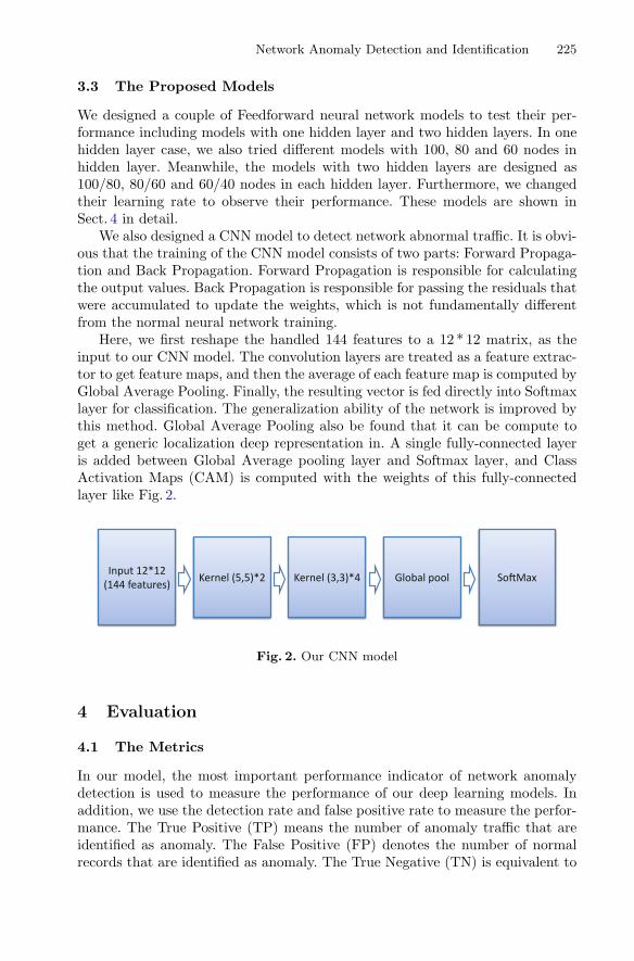
Network Anomaly Detection and Identification 225
3.3 The Proposed Models
We designed a couple of Feedforward neural network models to test their per-formance including models with one hidden layer and two hidden layers. In onehidden layer case, we also tried different models with 100, 80 and 60 nodes inhidden layer. Meanwhile, the models with two hidden layers are designed as100/80, 80/60 and 60/40 nodes in each hidden layer. Furthermore, we changedtheir learning rate to observe their performance. These models are shown inSect. 4 in detail.
We also designed a CNN model to detect network abnormal traffic. It is obvi-ous that the training of the CNN model consists of two parts: Forward Propaga-tion and Back Propagation. Forward Propagation is responsible for calculatingthe output values. Back Propagation is responsible for passing the residuals thatwere accumulated to update the weights, which is not fundamentally differentfrom the normal neural network training.
Here, we first reshape the handled 144 features to a 12 * 12 matrix, as theinput to our CNN model. The convolution layers are treated as a feature extrac-tor to get feature maps, and then the average of each feature map is computed byGlobal Average Pooling. Finally, the resulting vector is fed directly into Softmaxlayer for classification. The generalization ability of the network is improved bythis method. Global Average Pooling also be found that it can be compute toget a generic localization deep representation in. A single fully-connected layeris added between Global Average pooling layer and Softmax layer, and ClassActivation Maps (CAM) is computed with the weights of this fully-connectedlayer like Fig. 2.
Input 12*12 (144 features) Kernel (5,5)*2 Kernel (3,3)*4 Global pool So Max
Fig. 2. Our CNN model
4 Evaluation
4.1 The Metrics
In our model, the most important performance indicator of network anomalydetection is used to measure the performance of our deep learning models. Inaddition, we use the detection rate and false positive rate to measure the perfor-mance. The True Positive (TP) means the number of anomaly traffic that areidentified as anomaly. The False Positive (FP) denotes the number of normalrecords that are identified as anomaly. The True Negative (TN) is equivalent to

226 M. Zhu et al.
those correctly admitted, and it means the number of normal traffic that areidentified as normal. The False Negative (FN) denotes the number of anomalytraffic that are identified as normal. Table 3 shows the definition of confusionmatrix. We have the following notation:
Table 3. Confusion matrix
Predicted class
Actual class Anomaly Normal
Anomaly TP FN
Normal FP TN
Accuracy: the percentage of the number of records classified correctly versustotal the records shown below.
AC =TP + TN
TP + TN + FP + FN
True Positive Rate (TPR): as the equivalent of the Detection Rate (DR), itshows the percentage of the number of records identified correctly over the totalnumber of anomaly records, as shown below.
TPR =TP
TP + FN
False Positive Rate (FPR): the percentage of the number of records rejectedincorrectly is divided by the total number of normal records, as shown below.
FPR =FP
FP + TN
Hence, the motivation for the network anomaly detection models is to obtaina higher accuracy and detection rate with a lower false positive rate.
4.2 Experimental Results
In this paper, we used one of the most current and popular deep learning frame-works - Tensorflow [6]. Tensorflow is an excellent machine learning frameworkbelonging to Google. Its powerful capabilities enable researchers to create themachine learning models they designed more simply. The experiment is per-formed on a server, with a configuration of an Intel Xeon E5-2630 v3 (15MCache, 2.40 GHz) and 32GB memory. Some experiments have been designed tostudy the performance of our two different models for five-category classifica-tion, such as Normal, DoS, R2L, U2R and Probe. In order to demonstrate theefficiency of the proposed models, we also compare the results with several clas-sical machine learning algorithms, such as J48, Naive Bayes, NB Tree, RandomForest, Random Tree and SVM.

Network Anomaly Detection and Identification 227
FNN Model. Figure 3 shows the training process on KDDTrain+ and testingprocess on KDDTest+ and KDDtest21. From the figure, we can see the accu-racy rapidly rise before about 3000 epochs and gradually tend to flatten outafter about 15000 epochs. Furthermore, the accuracy on the training dataset isthe highest which is close to 1, it is because the model is trained from the samedataset directly and captures all the anomaly characteristics. While the detec-tion accuracy on dataset KDDTest+ and KDDTest21 are about 80%, and 50%respectively. The accuracy on KDDTest21 is lower than KDDTest+. It is becauseKDDTest21 removes all the anomalies that can be easily detected, resulting ina low detection accuracy.
0 5000 10000 15000 200000
0.2
0.4
0.6
0.8
1
Epoch Num
Accu
racy
Acc on KDDTrain+
Acc on KDDTest+
Acc on KDDTest21
Fig. 3. The Accuracy of FNN
Table 4 shows the accuracy with different FNN models. In the five-categoryclassification experiments, different kinds of Feedforward Neural Network wastested. The parameters include number of hidden layers, number of nodes in eachlayer and the learning rate of algorithm. As we can see, the best result 80.34%shows when there are 100 nodes in hidden layer, meanwhile the learning rate is0.5. When the number of nodes below 100, as nodes increase, there is a raisingtendency for precision. However, when we add the node number to 120, theprecious comes to a slightly drop. Results are getting complicated when it comesto the Feedforward Neural Network with two hidden layers. We can’t describe aobvious rule under such circumstances, just think a little lower performance thanthe Feedforward Neural Network with just one hidden layer. However, there is

228 M. Zhu et al.
Table 4. The accuracy with different FNN models
Structure Learning rate Accuracy
Hidden layer nodes = 120 0.5 78.9%
Hidden layer nodes = 100 0.5 80.34%
Hidden layer nodes = 80 0.5 80.01%
Hidden layer nodes = 60 0.5 76.75%
Hidden layer nodes = 100 0.8 80.18%
Hidden layer nodes = 100 0.1 77.57%
Hidden layer nodes = 100 * 80 0.5 79.2%
Hidden layer nodes = 80 * 60 0.5 78.8%
Hidden layer nodes = 60 * 40 0.5 79.01%
also a nice result (80.3%) when first hidden layer has 80 nodes and the secondhidden layer has 60 nodes with 0.8 learning rate.
CNN Model. Table 5 shows the detection result for CNN model. For CNN, wecan not design the enough layers since the hardware limitation. As a result, wejust tried a simple model with a drop optimization and it reaches an result thataccuracy comes to 77.8%. We also find the accuracy of CNN model is insensitivewith the size of kernel, number of full connect layer nodes and learning rate.Compared with FNN model, the accuracy of CNN is relatively lower. The reasonis that the connection among the features in the dataset may not be so strong.Another possible reason may be the layer is not deep enough.
4.3 Comparison with Other Methods
To make our results more intuitive, we used another famous classic machinelearning framework - scikit-learn to implement J48, Naive Bayes, NB Tree Ran-dom Forest, Random Tree and SVM on the same benchmark dataset. Theresults of the experiment are described in the Fig. 4. Compared with these classicmachine learning methods, the performance of deep learning algorithms showsa remarkable improvement. The classical machine learning algorithms generallyachieve about 75% accuracy, and the best NB tree reached 75.22% accuracy.However, the deep learning models can achieve at least 77.8% accuracy, and thebest one comes to 80.34% accuracy.
Table 6 shows the result for the Feedforward Neural Network on testingset KDDTest+ in the five-category classification experiments. The model hasachieved considerable results in the recognition of DOS and probe, but not goodin the rest two categories. When look at the dataset in Table 2, we find theanomaly U2R has few samples in both training set and testing set, so the accu-racy is greatly affected. While the anomaly R2L have enough samples in testingset whereas have few samples in training set, the data in the testing set is about

Network Anomaly Detection and Identification 229
Table 5. The accuracy with different CNN models
Structure Learning rate Accuracy
Convolutional neural network 0.5 74.38%
Kernel1(5,5)*2
Kernel2(3,3)*4
Full connect layer nodes = 120
Convolutional neural network 0.5 77.80%
Kernel1(5,5)*2
Kernel2(3,3)*4
Full connect layer nodes = 100
Convolutional neural network 0.5 74.40%
Kernel1(5,5)*2
Kernel2(3,3)*4
Full connect layer nodes = 80
Convolutional neural network 0.5 77.64%
Kernel1(5,5)*2
Kernel2(3,3)*4
Full connect layer nodes = 60
Convolutional neural network 0.1 70.83%
Kernel1(5,5)*2
Kernel2(3,3)*4
Full connect layer nodes = 100
Convolutional neural network 0.8 74.49%
Kernel1(5,5)*2
Kernel2(3,3)*4
Full connect layer nodes = 100
Convolutional neural network 0.5 74.84%
Kernel1(4,4)*2
Kernel2(2,2)*4
Full connect layer nodes = 100
Convolutional neural network 0.5 74.63%
Kernel1(7,7)*2
Kernel2(5,5)*4
Full connect layer nodes = 100
3 times of the training set. A small amount of training data can not produce amodel with sufficient generalization capability, resulting in low detection rate.Furthermore, the FPR of R2L and U2R are very low at the same time, whichshows these models have excellent ability to identify the subclasses trained bytraining set and the subclasses which could not be identified may be these classes

230 M. Zhu et al.
0.00% 10.00% 20.00% 30.00% 40.00% 50.00% 60.00% 70.00% 80.00% 90.00%
J48
Naïve Bayes
NB Tree
Random Forest
Random Tree
SVM
Feedforward Neural Network
CNN
J48 Naïve Bayes NB Tree Random Forest Random Tree SVMFeedforward
NeuralNetwork
CNN
KDDTest21 50.87% 54.77% 55.20% 50.60% 49.50% 50.65% 57.36% 56.79%KDDTest+ 74.35% 74.32% 75.22% 74.00% 72.50% 73.68% 80.34% 77.80%
KDDTest21 KDDTest+
Fig. 4. Comparartion in different machine learning algorithm
Table 6. The detection results for different anomaly types
Anomaly type FPR(%) DR(%)
DoS 2.04 83.44
R2L 0.79 24.52
U2R 0.07 10.30
Probe 2.17 82.34
containing no or just a few samples in the training set. As a result, the deeplearning models is practical for network anomaly detection.
5 Discussion
Based on the same benchmark, using KDDTrain+ as the training set andKDDTest+ and KDDTest-21 as the testing set, the experimental results showthat the network anomaly detection models both have higher accuracy than theother machine learning methods. In addition, there’s still a lot of space for theimprovement of network anomaly detection using deep learning.
First of all, we should refine this model’s pertinence to the specific aspect.As Robin Sommer mention [7], we should keep the scope narrow. Due to thediversity of network traffic, we should not have the idea that design a model

Network Anomaly Detection and Identification 231
which can detect all types of anomalies. Oppositely, a model which can detectthe specific anomalies under specific environment should be established. Thesemodels may not require strong generalization and migration capabilities, butwe can draw on the thought of boosting and bagging, which means overlay andintegrate these models to become a model detecting different anomalies in oneenvironment, this can cause the weakness of generalization ability to a certainextent. For example, we can design different models to detect DoS anomaly andU2R anomaly, then we use these models sequentially to get the result of eachanomaly. At last we combine the two results comprehensively to achieve the finalresult. We believe this could reach a better result than a general model.
Meanwhile, we can not test a deep enough CNN model because of the limi-tation of hardware. The huge amount of practice in different areas confirm thebig effect on CNN. It avoids explicit feature extraction and implicitly learnsfrom training data, this guarantee it can learn the inherent relation in features.When solute anomaly detection problem (whose essential issue is the classifica-tion problem), we are confident of the better performance CNN will show whenwe use the new device.
6 Related Work
Network anomaly detection is an important and dynamic research area. Manynetwork anomaly detection methods and systems have been proposed in theliterature.
Duffield et al. [8] proposed a rule-based anomaly detection on the IP networkwhich correlates the packet and flow level information. Cherkasova et al. [9] pre-sented an integrated framework of using regression based transaction modelsand application performance signatures to detect anomalous application behav-ior. Sharma et al. [10] used the Auto-Regressive models and a time-invariantrelationships based approach to detect the fault. Pannu et al. [11] presentedan adaptive anomaly detection framework that can self adapt by learning fromobserved anomalies at runtime. Tan et al. presented two anomaly predictionsystems PREPARE [12] and ALERT [13] that integrate online anomaly pre-diction, learning-based cause inference, and predictive prevention actuation tominimize the performance anomaly penalty without human intervention. Theyalso investigated the anomalous behavior of three datasets [14]. Bronevetsky etal. [15] designed a novel technique that combine classification algorithms withinformation on the abnormality of application behavior to improve detection.Gu et al. [16] developed an attack detection system LEAPS based on supervisedstatistical learning to classify benign and malicious system events. Tati et al.[17] proposed an algorithm to efficiently diagnose large-scale clustered failuresin computer networks which is based on greedy approach. Besides, several worksfocus on the anomaly/fault pattern analysis. Birke et al. [18] conducted a failurepattern analysis on 10K virtual and physical machines hosted on five commercialdatacenters over an observation period of one year. Their objective is to estab-lish a sound understanding of the differences and similarities between failures of

232 M. Zhu et al.
physical and virtual machines. Rosa et al. [19] studied three types of unsuccessfulexecutions in traces of a Google datacenter, namely fail, kill, and eviction. Theirobjective is to identify their resource waste, impacts on application performance,and root causes.
Most recently, with fast development of deep learning, there is a trend touse deep learning on network anomaly detection. Maimo et al. [20] used deeplearning method for anomaly detection in 5G networks. Tang et al. [21] applieda deep learning approach for flow-based anomaly detection in an SDN environ-ment. They just use six basic features (that can be easily obtained in an SDNenvironment) taken from the forty-one features of NSL-KDD Dataset. Yin et al.[22] proposed a deep learning approach for intrusion detection using recurrentneural networks (RNN). Javaid et al. [23] used Self-taught Learning (STL), adeep learning based technique, to develop a Network Intrusion Detection System.Roy et al. [24] used Deep Neural Network as a classifier for the different typesof intrusion attacks and did a comparative study with Support Vector Machine(SVM). Li et al. [25] proposed a image conversion method of NSL-KDD dataand evaluated the performance of the image conversion method by binary classclassification experiments.
In comparison, this paper applies feedforward neural network model andconvolutional neural network model for network anomaly detection and studiesthe impact of different model parameters. We also perform a detailed compar-ison of detection accuracy with several traditional machine learning methodsand demonstrate the deep learning based detection models can achieve a betteraccuracy.
7 Conclusion
This paper presents a new anomaly detection method based on deep learningmodels, specifically the feedforward neural network (FNN) model and convolu-tional neural network (CNN) model. The performance of the models is evaluatedby several experiments with a popular NSL-KDD dataset. From the experimen-tal results, we find the FNN and CNN models not only have a strong modelingability for network anomaly detection, but also have relatively high accuracy.Compared with several traditional machine learning methods, such as J48, NaiveBayes, NB Tree, Random Forest, Random Tree and SVM, the proposed mod-els obtain a higher accuracy and detection rate with lower false positive rate.The deep learning models can effectively improve both the detection accuracyand the ability to identify the anomaly types. With the continuous advancementof deep learning technology and the development of hardware accelerators, webelieve better performance can be achieved in network anomaly detection byusing deep learning methods in the future.
Acknowledgments. This work is supported by the National Basic Research Programof China (Grant No. 2015CB352400), National Natural Science Foundation of China(Grant No. 61702492, U1401258), and Shenzhen Basic Research Program (Grant No.JCYJ20170818153016513, JCYJ20170307164747920).

Network Anomaly Detection and Identification 233
References
1. Benson, T., Akella, A., Maltz, D.A.: Network traffic characteristics of data centersin the wild. In: Proceedings of the 10th ACM SIGCOMM Conference on InternetMeasurement, pp. 267–280. ACM (2010)
2. Gill, P., Jain, N., Nagappan, N.: Understanding network failures in data centers:measurement, analysis, and implications. In: ACM SIGCOMM Computer Com-munication Review, vol. 41, no. 4, pp. 350–361. ACM (2011)
3. Bhuyan, M.H., Bhattacharyya, D.K., Kalita, J.K.: Network anomaly detection:methods, systems and tools. IEEE Commun. Surv. Tutor. 16(1), 303–336 (2014)
4. Kwon, D., Kim, H., Kim, J., Suh, S.C., Kim, I., Kim, K.J.: A survey of deeplearning-based network anomaly detection. Clust. Comput. 1–13 (2017)
5. Nsl-kdd dataset (2018). http://www.unb.ca/cic/datasets/nsl.html6. Abadi, M., Barham, P., Chen, J., Chen, Z., Davis, A., Dean, J., Devin, M., Ghe-
mawat, S., Irving, G., Isard, M., et al.: Tensorflow: a system for large-scale machinelearning. In: OSDI, vol. 16, pp. 265–283 (2016)
7. Sommer, R., Paxson, V.: Outside the closed world: on using machine learning fornetwork intrusion detection. In: IEEE Symposium on Security and Privacy (SP),pp. 305–316. IEEE (2010)
8. Duffield, N., Haffner, P., Krishnamurthy, B., Ringberg, H.: Rule-based anomalydetection on Ip flows. In: INFOCOM (2009)
9. Cherkasova, L., Ozonat, K., Mi, N., Symons, J., Smirni, E.: Anomaly? applicationchange? or workload change? towards automated detection of application perfor-mance anomaly and change. In: DSN (2008)
10. Sharma, A.B., Chen, H., Ding, M., Yoshihira, K., Jiang, G.: Fault detection andlocalization in distributed systems using invariant relationships. In: DSN (2013)
11. Pannu, H.S., Liu, J., Fu, S.: AAD: adaptive anomaly detection system for cloudcomputing infrastructures. In: SRDS (2012)
12. Tan, Y., Nguyen, H., Shen, Z., Gu, X., Venkatramani, C., Rajan, D.: Prepare: pre-dictive performance anomaly prevention for virtualized cloud systems. In: ICDCS(2012)
13. Tan, Y., Gu, X., Wang, H.: Adaptive system anomaly prediction for large-scalehosting infrastructures. In: PODC (2010)
14. Tan, Y., Gu, X.: On predictability of system anomalies in real world. In: MASCOTS(2010)
15. Bronevetsky, G., Laguna, I., De Supinski, B.R., Bagchi, S.: Automatic fault char-acterization via abnormality-enhanced classification. In: DSN (2012)
16. Gu, Z., Pei, K., Wang, Q., Si, L., Zhang, X., Xu, D.: Leaps: detecting camouflagedattacks with statistical learning guided by program analysis. In: DSN (2015)
17. Tati, S., Ko, B.J., Cao, G., Swami, A., Porta, T.L.: Adaptive algorithms for diag-nosing large-scale failures in computer networks. In: DSN (2012)
18. Birke, R., Giurgiu, I., Chen, L.Y., Wiesmann, D., Engbersen, T.: Failure analysisof virtual and physical machines: patterns, causes and characteristics. In: DSN(2014)
19. Rosa, A., Chen, L.Y., Binder, W.: Understanding the dark side of big data clusters:an analysis beyond failures. In: DSN (2015)
20. Maimo, L.F., Gomez, A.L.P., Clemente, F.J.G., Perez, M.G., Perez, G.M.: A self-adaptive deep learning-based system for anomaly detection in 5G networks. IEEEAccess 6, 7700–7712 (2018)

234 M. Zhu et al.
21. Tang, T.A., Mhamdi, L., McLernon, D., Zaidi, S.A.R., Ghogho, M.: Deep learn-ing approach for network intrusion detection in software defined networking. In:2016 International Conference on Wireless Networks and Mobile Communications(WINCOM), pp. 258–263. IEEE (2016)
22. Yin, C., Zhu, Y., Fei, J., He, X.: A deep learning approach for intrusion detectionusing recurrent neural networks. IEEE Access 5, 21954–21961 (2017)
23. Javaid, A., Niyaz, Q., Sun, W., Alam, M.: A deep learning approach for net-work intrusion detection system. In: Proceedings of the 9th EAI InternationalConference on Bio-inspired Information and Communications Technologies (for-merly BIONETICS). ICST (Institute for Computer Sciences, Social-Informaticsand Telecommunications Engineering), pp. 21–26 (2016)
24. Roy, S.S., Mallik, A., Gulati, R., Obaidat, M.S., Krishna, P.V.: A deep learn-ing based artificial neural network approach for intrusion detection. In: Giri, D.,Mohapatra, R.N., Begehr, H., Obaidat, M.S. (eds.) ICMC 2017. CCIS, vol. 655,pp. 44–53. Springer, Singapore (2017). https://doi.org/10.1007/978-981-10-4642-1 5
25. Li, Z., Qin, Z., Huang, K., Yang, X., Ye, S.: Intrusion detection using convolutionalneural networks for representation learning. In: Liu, D., Xie, S., Li, Y., Zhao, D.,El-Alfy, E.-S.M. (eds.) ICONIP 2017. LNCS, vol. 10638, pp. 858–866. Springer,Cham (2017). https://doi.org/10.1007/978-3-319-70139-4 87
A Feedback Prediction Modelfor Resource Usage and Offloading Time
in Edge Computing
Menghan Zheng1, Yubin Zhao1(B), Xi Zhang1, Cheng-Zhong Xu1,and Xiaofan Li2
1 Shenzhen Institutes of Advanced Technology, Chinese Academy of Sciences,Shenzhen 518055, China
{zhengmh,zhaoyb,xi.zhang,cz.xu}@siat.ac.cn2 Shenzhen Institute of Radio Testing and Technology, Shenzhen 518048, China
Abstract. Nowadays, edge computing which provides low delay ser-vices has gained much attention in the research filed. However, the lim-ited resources of the platform make it necessary to predict the usage,execution time exactly and further optimize the resource utilization dur-ing offloading. In this paper, we propose a feedback prediction model(FPM), which includes three processes: the usage prediction process, thetime prediction process and the feedback process. Firstly, we use averageusage instead of instantaneous usage for usage prediction and calibratethe prediction results with real data. Secondly, building the time pre-diction process with the predicted usage values, then project the timeerror to usage value and update the usage values. Meanwhile, our modelre-executes the time prediction process. Thirdly, setting a judgment andfeedback number to the correction process. If prediction values meetthe requirement or reach the number, FPM stops error feedback andskips to the next training. We compare the testing results to other twomodel which are BP neural network and FPM without feedback process(NO-FP FPM). The average usage and time prediction errors of BP andNO-FP FPM are 10%, 25% and 16%, 12%. The prediction accuracy inFPM has a great improvements. The average usage prediction errors canreach less than 8% and time error reach about 6%.
Keywords: Computation offloading · Resource optimizationTime prediction · Back propagation · Feedback process
1 Introduction
According to Internet Data Center (IDC), the market prospect of edge comput-ing is very broad. And nearly 40% of IoT data will be processed near the clients
Y. Zhao—This work was supported by the China National Basic Research Program(973 Program, No. 2015CB352400), National Nature Science Foundation of China(Grand No. 61501443), NSFC under grand U1401258.
c© Springer International Publishing AG, part of Springer Nature 2018M. Luo and L.-J. Zhang (Eds.): CLOUD 2018, LNCS 10967, pp. 235–247, 2018.https://doi.org/10.1007/978-3-319-94295-7_16

236 M. Zheng et al.
with the use of fog computing and edge computing by 2018 [1]. Depending onthe increasing edge devices and users’ requirements which include real-time, highefficiency and short delay, edge computing is quite suitable for IoT systems [2,3].However, power consumption, storage and bandwidth size of the edge platformare limited comparing to the cloud data centers. Therefore, edge computing isnot suitable for complex tasks and the importance of resource utilization.
In the process of services providing in edge computing, platform firstlyreceives the service requests, then determine the service order according to thecorresponding rules of the platform. Afterwards, the platform allocates resourcefor each task [6,7]. Lastly, the platform returns the results to the requestingdevices after the computing nodes complete computation process. In general,the response times are regarded as a criterion for evaluating the performanceof the platform [5]. On the condition of the limited hardware capability of theplatform, we can only improve the response ability through the optimizationof resource utilization. In this case, we need to know the resource requirementsof each task before the allocation of resources. Then the platform can give thereasonable allocation base on the expected execution time and current state ofresource utilization. Meanwhile we obtain the real execution time to help us howto allocate the resources. Therefore the accuracy of execution time predictionand resource requirement are essential in resource allocation.
In this paper, we propose a feedback prediction model (FPM) which is usedfor resource usage prediction and offloading time prediction. These predictionscan be used as references and will benefit resource allocation in edge comput-ing. Time prediction is for the queueing management and division of differentcategories of tasks. Firstly, we calculate usage by accumulating the resourceconsumption in the execution time. However curve of resource consumption isdifficult to solve, so we give the usage prediction through the average resourceconsumption and correction base on real usage data. Secondly, we combine thetransmission time and predicted usage to give the time prediction model. Thirdly,building a feedback process after we get the time prediction error. The time pre-dicted error will be mapped to the resource usage. During the feedback process,the weights of usage and time prediction model will update until the time errorreach our setting threshold or greater than upper bound which is used to pre-vent the divergence caused by feedback. The main contributions of this paperare listed as follows.
(1) We propose a resource usage prediction model. Because the dynamic changecurve of usage is difficult to express, predicted usage is obtained by averagepredicted usage.
(2) We integrate the predicted usage and transmission time to build the timeprediction model, then calculate the time error.
(3) We design the backward propagation method, time error’s feedback andusage’s correction to update the predicted weights. Then we set the stoppingcondition of the feedback loop to promise efficiency of feedback process.
The rest of the paper is organized as follows: Sect. 2 introduces some relatedwork. In Sect. 3, we describe the architecture of the prediction model and

A Feedback Prediction Model for Offloading Time in Edge Computing 237
introduce the three constituent processes of FPM. In Sect. 4, the simulationresults are presented. Finally, the conclusion is given in Sect. 5.
2 Related Work
Research on resource optimization based on cloud computing has been goingon for many years. At present, the role which edge computing plays in the IoThas become more and more important. Low network delay make it suitablefor applications which demand high performance of real time. In addition, net-work slicing and edge computing are the key technologies in 5G network [8].However, the disadvantage is the limited computing power and limited carryingcapacity. Meanwhile, for lightweight loads, if you need the platform executes theoffloading tasks fast and efficient, the problem of resource optimization has beenhighlighted. And accurate prediction is an important part of the optimizationproblem.
In early 2003, AKAMAI which is a provider of content distribution network,CDN and cloud services had been cooperated with IBM on edge computing.Many network companies represented by CISCO are mainly based on fog com-puting [4]. Strictly speaking, there is no essential difference between fog com-puting and edge computing, they are both provide a nearby calculation. Up tilltoday, several existing research attempts to find the best resource matching, inorder to achieve better resource utilization. The common practice is establishinga prediction model from hundreds of thousands of test data. And they alwayschoose the Artificial Neural Network (ANN) or other training models of artificialintelligence as prototype of the prediction model.
In [9], Markov chain model and linear regression are used to predict theCPU and memory utilizations, moreover, Markov chain model in [10,11] consid-ers both current and future resource utilization to predict the future utilizationand give the usage prediction. In [12], they develop a heuristic algorithm whichis based on Artificial Fish Swam Algorithm (AFSA) to solve the energy opti-mization problem. The prediction model in [13] is built by Fuzzy InformationGranulation (FIG) and Support Vector Regression (SVR). The main work of [14]focus on resource prediction engines (RPEs) and epidemic models. The authorsin [15] establish the prediction algorithm based on BP neural network. Besides,there are another methods used to predict the resource usage and optimal alloca-tion, such as Simulated Annealing Algorithm (SA) in [16], GEO-CLUSTERINGALGORITHM in [17], Deep Learning Approach in [18] and so on.
3 Prediction Model
3.1 Architecture Description
In order to give accurate prediction of execution time, we proposed a predictionmodel which is called feedback prediction model (FPM). In this model, it com-bines most affected factors which may bring strong influence to execution time,
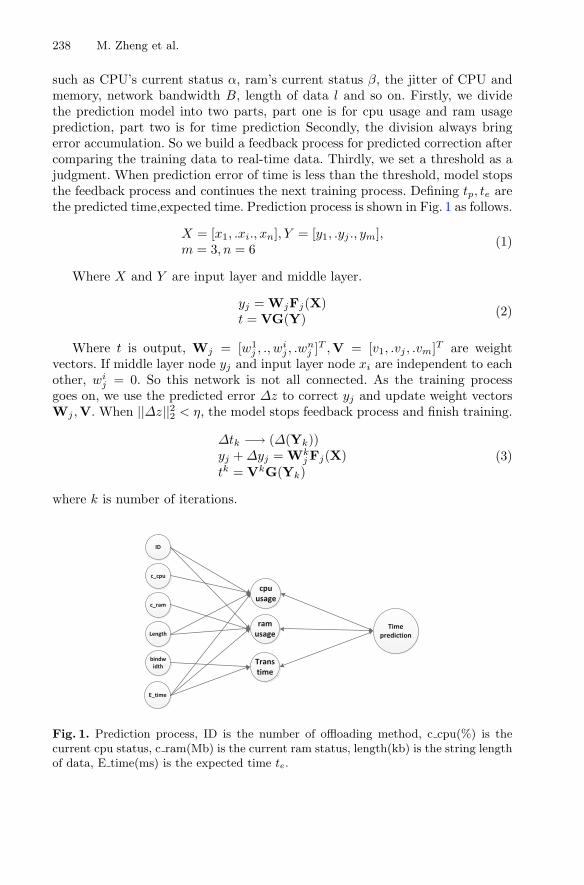
238 M. Zheng et al.
such as CPU’s current status α, ram’s current status β, the jitter of CPU andmemory, network bandwidth B, length of data l and so on. Firstly, we dividethe prediction model into two parts, part one is for cpu usage and ram usageprediction, part two is for time prediction Secondly, the division always bringerror accumulation. So we build a feedback process for predicted correction aftercomparing the training data to real-time data. Thirdly, we set a threshold as ajudgment. When prediction error of time is less than the threshold, model stopsthe feedback process and continues the next training process. Defining tp, te arethe predicted time,expected time. Prediction process is shown in Fig. 1 as follows.
X = [x1, .xi., xn], Y = [y1, .yj ., ym],m = 3, n = 6 (1)
Where X and Y are input layer and middle layer.
yj = WjFj(X)t = VG(Y) (2)
Where t is output, Wj = [w1j , ., wi
j , .wnj ]T ,V = [v1, .vj , .vm]T are weight
vectors. If middle layer node yj and input layer node xi are independent to eachother, wi
j = 0. So this network is not all connected. As the training processgoes on, we use the predicted error Δz to correct yj and update weight vectorsWj ,V. When ||Δz||22 < η, the model stops feedback process and finish training.
Δtk −→ (Δ(Yk))yj + Δyj = Wk
jFj(X)tk = VkG(Yk)
(3)
where k is number of iterations.
Fig. 1. Prediction process, ID is the number of offloading method, c cpu(%) is thecurrent cpu status, c ram(Mb) is the current ram status, length(kb) is the string lengthof data, E time(ms) is the expected time te.
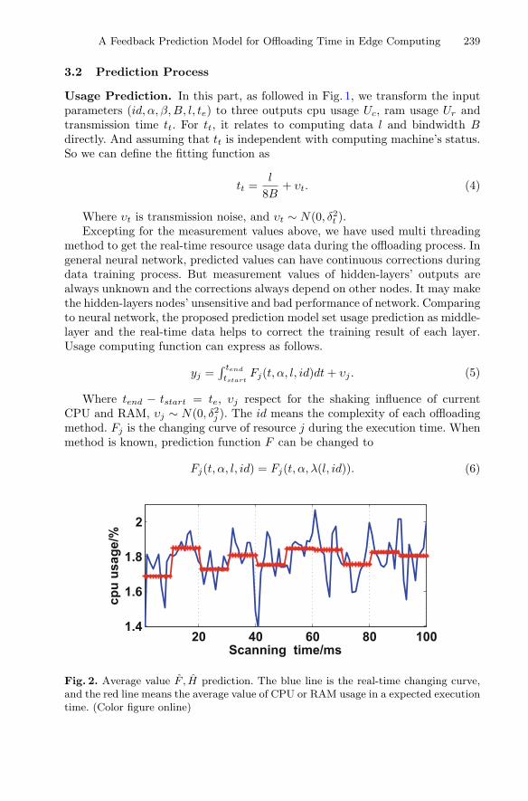
A Feedback Prediction Model for Offloading Time in Edge Computing 239
3.2 Prediction Process
Usage Prediction. In this part, as followed in Fig. 1, we transform the inputparameters (id, α, β,B, l, te) to three outputs cpu usage Uc, ram usage Ur andtransmission time tt. For tt, it relates to computing data l and bindwidth Bdirectly. And assuming that tt is independent with computing machine’s status.So we can define the fitting function as
tt =l
8B+ υt. (4)
Where υt is transmission noise, and υt ∼ N(0, δ2t ).Excepting for the measurement values above, we have used multi threading
method to get the real-time resource usage data during the offloading process. Ingeneral neural network, predicted values can have continuous corrections duringdata training process. But measurement values of hidden-layers’ outputs arealways unknown and the corrections always depend on other nodes. It may makethe hidden-layers nodes’ unsensitive and bad performance of network. Comparingto neural network, the proposed prediction model set usage prediction as middle-layer and the real-time data helps to correct the training result of each layer.Usage computing function can express as follows.
yj =∫ tend
tstartFj(t, α, l, id)dt + υj . (5)
Where tend − tstart = te, υj respect for the shaking influence of currentCPU and RAM, υj ∼ N(0, δ2j ). The id means the complexity of each offloadingmethod. Fj is the changing curve of resource j during the execution time. Whenmethod is known, prediction function F can be changed to
Fj(t, α, l, id) = Fj(t, α, λ(l, id)). (6)
20 40 60 80 1001.4
1.6
1.8
2
Scanning time/ms
cpu
usag
e/%
Fig. 2. Average value F , H prediction. The blue line is the real-time changing curve,and the red line means the average value of CPU or RAM usage in a expected executiontime. (Color figure online)

240 M. Zheng et al.
Where λ is the computation function. When the training process start, Fj
will be given. Meanwhile the usage can be evaluated through definite integral.However, because of the shaking characteristics and changing regular of CPU,Fj are difficult to training or the rule of change curves is not obvious in unittime as depicted in Fig. 2. Thus, we use average value F of cpu status instead ofF during each offloading process. The predicted value are given as
yj = Fj • te + υj . (7)
Where Fj are the average value of cpu status and ram status, yj are the pre-dicted values. And we transform the training targets from yj to Fj . For trainingnumber N , the training inputs and outputs are the (yj−υc)
te, F . Conversely, real
execution time probably not equals the expected time. Therefore Fj need correc-tions ΔFj to reach the expected value. Defining predicted average usage valuesFj = Fj +ΔFj . According to test, the cpu usage and ram usage follow the Gaussdistribution N(y0
j , (σcj)
2). So the best training result F oj can be given as
E(yj) = y0j = te ∗ E(F o
j )
D(F oj ) = D(yj)+(σc
j )2
t2e
F oj ∼ N(y0
j
te,
D(yj)+(σcj )
2
t2e)
(8)
Where y0j are the expected value of measurement values yj . Defining predicted
values as yj , cpu usage predicted error Δyj = yj − yj , E(Δyj) = 0,D(Δyj) =(δΔ
j )2.Δyj = g(te)ΔFj = Δyj
te
(9)
The final predicted function can be given as
yj = (Fj + ΔFj) • te + υj . (10)
Besides, E(ΔFj) = 0, performance evaluation are given like
E(yj) = y0j ,
D(yj) = t2e ∗ D(Fj) + (δΔj )2 + δ2j
(11)
Time Prediction. When the model finish the usage training, we can useresource usage to predict offloading time to. The offloading process includes twoindependent parts, one is data transition time tt, another is the execution timetx. So
to = tx + tt + υt (12)
Where υt is the transition noise. tx relates to Y = [y1, yj , ym].
tx = VG(Y)Δt = tx − txΔt = ΔVG(Y)
(13)

A Feedback Prediction Model for Offloading Time in Edge Computing 241
Where tx is the predicted time, Δt is prediction error, tx is the real executiontime, ΔV is adjust weights vector.
Feedback Process. When forward propagation process finish, feedback processstart back propagation. From part two, we can obtain the predicted error Δt. Inpart one, predicted usage yk
j change to
ykj = (Fj + ΔFj) • (te + Δtj) (14)
Then feedback process start back propagation and correct the usage predictions.Meanwhile weights of usage prediction model update by the corrections. So theusage correction can be given like
Δykj = (Fj + ΔFj) • Δtj (15)
Time prediction process will be re-execute after usage correction. Therefore timeprediction error Δt will be updated. If Δt > η, η is the given training threshold,model will go on back propagation and error feedback. Otherwise, when feedbackprocess satisfy the addition of Δt < η or reach the setting max training number,model will skip to next training. In addition, we give a max training thresholdρ to avoid the training divergence, if Δt > ρ, model stop back propagation.
The iterative process is as follows. Training flow chart is shown in Fig. 3.
Algorithm 1Input: X,YOutput: W,V1: for i ≤ P do2: yi
j = (F ij + ΔF i
j ) • tie
3: tix = ViG(Yi)4: Δti = tix − tix5: Δti = ΔVG(Yi)6: Vi = Vi + ΔV7: while ||Δti||22 > η && k < N do
8: yikj = (F ik
j + ΔF ikj ) • (tie + Δti)
9: yij + Δyik
j = Wkj F
ij(X
i)10: tk = VkG(Yk)11: Δtik = tie − tk
12: if ||Δtik||22 < ρ then13: ccontinue14: else15: break16: end if17: k + +18: end while19: end for

242 M. Zheng et al.
Fig. 3. Flow chat of FPM.
4 Experiment and Analysis
In order to test the performance of FPM, we set up FPM experiment systemto obtain the needing training data. Meanwhile the system include five testoffloading methods which are Optical Character Recognition (OCR), AES, SHA,MD5 (three encryption algorithms) and indoor localization method (GEO). Wemeasured all parameters mentioned in FPM and give performance comparisonwith BP neural network and FPM without feedback process (NO-FP FPM).
4.1 Performance of Usage Prediction
Usage predictions include cpu usage prediction and ram usage prediction. FromFigs. 4 and 5, we can see the predicted performance with three prediction mod-els which are FPM, NO-FP FPM, BP neural network. Comparing to the realdata, three models’ prediction errors are shown in Table 1. Besides, each methodhas different requirements for memory and CPU. It always depends on its ownalgorithm complexity and the length of the processed data.

A Feedback Prediction Model for Offloading Time in Edge Computing 243
AES MD5 SHA GEO OCR0
20
40
60
80
100
120
Offloading methods
RA
M u
sage
/(Mb)
realFPMNO−FP FPMBP
Fig. 4. Comparison of RAM usage prediction.
AES MD5 SHA GEO OCR0
1
2
3
4
5
6
Offloading method
CPU
usa
ge/(%
)
realFPMNO−FP FPMBP
Fig. 5. Comparison of CPU usage prediction.
Table 1. Comparison of usage prediction errors.
Kind Method AES (%) MD5 (%) SHA (%) GEO (%) OCR (%)
CPU FPM 0.87 3.56 3.54 10.30 1.31
CPU NO-FP FPM 15.34 33.90 12.90 22.89 12.48
CPU BP 5.43 6.21 24.35 16.82 6.57
RAM FPM 5.56 6.27 4.38 6.25 3.31
RAM NO-FP FPM 24.07 30.69 40.07 93.75 44.19
RAM BP 20.37 41.58 44.47 156.25 16.57
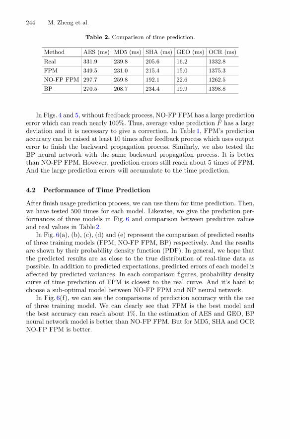
244 M. Zheng et al.
Table 2. Comparison of time prediction.
Method AES (ms) MD5 (ms) SHA (ms) GEO (ms) OCR (ms)
Real 331.9 239.8 205.6 16.2 1332.8
FPM 349.5 231.0 215.4 15.0 1375.3
NO-FP FPM 297.7 259.8 192.1 22.6 1262.5
BP 270.5 208.7 234.4 19.9 1398.8
In Figs. 4 and 5, without feedback process, NO-FP FPM has a large predictionerror which can reach nearly 100%. Thus, average value prediction F has a largedeviation and it is necessary to give a correction. In Table 1, FPM’s predictionaccuracy can be raised at least 10 times after feedback process which uses outputerror to finish the backward propagation process. Similarly, we also tested theBP neural network with the same backward propagation process. It is betterthan NO-FP FPM. However, prediction errors still reach about 5 times of FPM.And the large prediction errors will accumulate to the time prediction.
4.2 Performance of Time Prediction
After finish usage prediction process, we can use them for time prediction. Then,we have tested 500 times for each model. Likewise, we give the prediction per-formances of three models in Fig. 6 and comparison between predictive valuesand real values in Table 2.
In Fig. 6(a), (b), (c), (d) and (e) represent the comparison of predicted resultsof three training models (FPM, NO-FP FPM, BP) respectively. And the resultsare shown by their probability density function (PDF). In general, we hope thatthe predicted results are as close to the true distribution of real-time data aspossible. In addition to predicted expectations, predicted errors of each model isaffected by predicted variances. In each comparison figures, probability densitycurve of time prediction of FPM is closest to the real curve. And it’s hard tochoose a sub-optimal model between NO-FP FPM and NP neural network.
In Fig. 6(f), we can see the comparisons of prediction accuracy with the useof three training model. We can clearly see that FPM is the best model andthe best accuracy can reach about 1%. In the estimation of AES and GEO, BPneural network model is better than NO-FP FPM. But for MD5, SHA and OCRNO-FP FPM is better.

A Feedback Prediction Model for Offloading Time in Edge Computing 245
250 300 350 400 4500
0.050.1
0.150.2
(a).Offloading Time(AES)/(ms)
150 200 250 300 350 4000
0.05
0.1
(b).Offloading Time(MD5)/(ms)
150 200 2500
0.05
0.1
0.15
0.2
(c).Offloading Time(SHA)/(ms)
10 20 30 400
0.05
0.1
0.15
0.2
(d).Offloading Time(GEO)/(ms)
1200 1300 1400 1500 16000
0.05
0.1
(e).Offloading Time(OCR)/(ms)
1 2 3 4 50
1020
304050
(f).Predition Model
Pred
ictio
n A
ccur
acy/
(%)
realFPMNO−FP FPMBP
realFPMNO−FP FPMBP
realFPMNO−FP FPMBP
realFPMNO−FP FPMBP
FPMNO−FP FPMBP
realFPMNO−FP FPMBP
Fig. 6. PDF comparation of three models.
5 Conclusion
In this paper, we propose a time prediction model (FPM) during the computationoffloading in edge computing platform. In FPM, we divide the model into twoparts, resource usage prediction and time prediction. In usage prediction part, wetransfer the predicted target from usage to average usage. In time prediction part,we utilize the training error to correct the predicted model and complete the backpropagation until the error reach the set threshold. Then we use the proposedmodel to do the prediction process and give the comparisons of predicted resultswith the other two models which are BP neural network and NO-FP FPM. Itshows a good performance and best accuracy can be less than 6%.
246 M. Zheng et al.
References
1. Yang, B., Chai, W.K., Xu, Z., Katsaros, K.V., Pavlou, G.: Cost-efficient NFV-enabled mobile edge-cloud for low latency mobile applications. IEEE Trans. Netw.Serv. Manag. 15(1), 475–488 (2018)
2. Barik, R.K., Dubey, H., Mankodiya, K.: SOA-FOG: secure service-oriented edgecomputing architecture for smart health big data analytics. In: 2017 IEEE GlobalConference on Signal and Information Processing (Global SIP), pp. 477–481. IEEEPress, New York (2018). https://doi.org/10.1109/SC2.2017.11
3. Premsankar, G., Di Francesco, M., Taleb, T.: Edge computing for the Internet ofThings: a case study. IEEE Internet Things J. 5, 1275–1284 (2018)
4. Baike for Edge Computing. http://baike.baidu.com/item/%E8%BE%B9%E7%BC%98%E8%AE%A1%E7%AE%97/9044985?fr=aladdin
5. Zhang, J., Xia, W., Yan, F., Shen, L.: Joint computation offloading and resourceallocation optimization in heterogeneous networks with moble edge computing.IEEE Access pp(99), 1 (2018)
6. Hao, Y., Chen, M., Hu, L., Hossain, M.S., Ghoneim, A.: Energy efficient taskcaching and offloading for mobile edge computing. IEEE Access Spec. Sect. Mob.Edge Comput. 6, 11365–11373 (2018)
7. Luo, C., Salinas, S., Li, M., Li, P.: Energy-effecient autonomic offloading in mobileedge computing. In: 15th International Conference on Dependable, Autonomic andSecure Computing, 15th International Conference on Pervasive Intelligence andComputing, 3rd International Conference on Big Data Intelligence and Computingand Cyber Science and Technology Congress, pp. 581–588. IEEE Press, New York(2017). https://doi.org/10.1109/DASC-PICom-DataCom-CyberSciTec.2017.104
8. Huang, S.-C., Luo, Y.-C., Chen, B.-L., Chung, Y.-C., Chou, J.: Application-awaretraffic redirection: a mobile edge computing implementation toward future 5G net-works. In: IEEE 7th International Symposium on Cloud and Service Computing,pp. 17–23. IEEE Press, New York (2017). https://doi.org/10.1109/SC2.2017.11
9. Xia, Y., Ren, R., Cai, H., Vasilakos, A.V., Lv, Z.: Daphne: a flexible and hybridscheduling framework in multi-tenant clusters. IEEE Trans. Netw. Serv. Manag.15(1), 330–343 (2018)
10. Melhem, S.B., Agarwal, A., Goel, N., Zaman, M.: Markov prediction model forhost load detection and VM placement in live migration. IEEE Access pp(21),7190–7205 (2018)
11. Yang, X., Chen, Z., Li, K., Sun, Y., Liu, N., Xie, W., Zhao, Y.: Communication-constrained mobile edge computing systems for wireless virtual reality: schedulingand tradeoff. IEEE Access 1–13 (2018)
12. Yang, L., Zhang, H., Li, M., Guo, J., Ji, H.: Mobile edge computing empoweredenergy efficient task offloading in 5G. IEEE Trans. Veh. Technol. pp(11), 1–12(2018)
13. Zhao, P., Tian, H., Fan, S., Paulraj, A.: Information prediction and dynamic pro-gramming based RAN slicing for mobile edge computing. IEEE Wirel. Commun.Lett. 1–4 (2018)
14. Kryftis, Y., Mastorakis, G., Mavromoustakis, C.X., Batall, J.M., Rodrigues,J.J.P.C., Dobre, C.: Resource usage prediction models for optimal multimedia con-tent provision. IEEE Syst. J. 11(4), 2852–2863 (2017)
15. Wang, X., Wang, X., Che, H., Li, K., Huang, M., Gao, C.: An intelligent economicapproach for dynamic resource allocation in cloud services. IEEE Trans. CloudComput. 3(3), 275–289 (2015)

A Feedback Prediction Model for Offloading Time in Edge Computing 247
16. Cao, Z., Lin, J., Wan, C., Song, Y., Zhang, Y., Wang, X.: Optimal cloud computingresource allocation for demand side management in smart grid. IEEE Trans. SmartGrid 8(4), 1943–1955 (2017)
17. Bouet, M., Conan, V.: Mobile edge computing resources optimization: a geo-clustering approach. IEEE Trans. Netw. Serv. Manag. (2018)
18. Yu, S., Wang, X., Langar, R.: Computation offloading for mobile edge computing:a deep learning approach. In: IEEE 28th Annual International Symposium onPersonal, Indoor, and Mobile Radio Communications (PIMRC), pp. 1–6 (2017)

Application and Industry Track: CloudService System

cuCloud: Volunteer Computingas a Service (VCaaS) System
Tessema M. Mengistu(B), Abdulrahman M. Alahmadi, Yousef Alsenani,Abdullah Albuali, and Dunren Che
Department of Computer Science, Southern Illinois University at Carbondale,Carbondale, USA
{tessema.mengistu,aalahmadi,yalsenani,aalbuali,dche}@siu.edu
Abstract. Emerging cloud systems, such as volunteer clouds and mobileclouds, are getting momentum among the current topics that dominatethe research landscape of Cloud Computing. Volunteer cloud computingis an economical, secure, and greener alternative solution to the currentCloud Computing model that is based on data centers, where tens ofthousands of dedicated servers are setup to back the cloud services. Thispaper presents cuCloud, a Volunteer Computing as a Service (VCaaS)system that is based on the spare resources of personal computers ownedby individuals and/or organizations. The paper addresses the design andimplementation issues of cuCloud, including the technical details of itsintegration with the well-known open source IaaS cloud managementsystem, CloudStack. The paper also presents the empirical performanceevidence of cuCloud in comparison with Amazon EC2 using a big-dataapplication based on Hadoop.
1 Introduction
Cloud Computing, the still fast growing and evolving technology, has kept draw-ing significant attention from both the computing industry and academia fornearly a decade. Extensive researches in Cloud Computing have resulted in thefulfillment of many of the promised characteristics, such as utility computing,pay-as-you-go, flexible (unlimited) capacity, etc. Emerging cloud systems suchas ad hoc and mobile clouds, volunteer clouds, federation of clouds, and hybridclouds are among the research topics that may jointly help to reshape the land-scape of future Cloud Computing – to better satisfy computing needs.
Currently, more than 4 billion users use the Internet1. Supercomputing sitesand large cloud data centers provide the infrastructures that host applicationslike Facebook and Twitter, which are accessed by millions2 of users concurrently.The current cloud infrastructures that are based on tens (if not hundreds) ofthousands of dedicated servers are expensive to setup; running the infrastructureneeds expertise, a lot of electrical power for cooling the facilities, and redundant1 http://www.internetworldstats.com/.2 http://www.internetlivestats.com/.
c© Springer International Publishing AG, part of Springer Nature 2018M. Luo and L.-J. Zhang (Eds.): CLOUD 2018, LNCS 10967, pp. 251–264, 2018.https://doi.org/10.1007/978-3-319-94295-7_17

252 T. M. Mengistu et al.
supply of everything in a data center to provide the desired resilience. Cloudservers, specialized infrastructure for fault tolerance, and the electricity con-sumption account for 45%, 25%, and 15% of the total amortized cost of a clouddata center, respectively [1]. The servers and the cooling system make up about80% of all the electricity consumption in a typical data center [2]. The high energyconsumption in data centers contributes to the environmental impact of globalwarming. Currently, the ICT industry contributes 2% of the total greenhousegases emission and the contribution of data centers to this emission is expectedto increase to 18% by 2020 [3]. On top of the costs and environmental factors, thecurrent “datacenter based” cloud infrastructures, even though well-provisionedand well-managed, are not suitable for some application scenarios. For instance,the inevitable concerns of cloud clients for “no control” on their confidentialdata and business logic can prohibit them from migrating their applications anddatasets to the clouds that are in the hands of third-parties. Self-provisioned,on-premise, private cloud can be a suitable solution to these users. However, theinitial investment for setting up such a private cloud infrastructure based on adedicated data center can be prohibitively expensive.
In addition to the vast number of dedicated servers setup in cloud data cen-ters, there are billions of Personal Computers (PCs) owned by individuals andorganizations worldwide. These PCs are underutilized, usually used only for a fewhours per day [4]. The computing power of these computers can be consolidatedas a huge cloud fabric and utilized as an alternative Cloud Computing solution,i.e., volunteer cloud computing. Volunteer cloud computing based on consolidat-ing the spare capacities of edge computing resources (within an organization orcommunity) and delivering on-premise private clouds is a rather economical andgreener alternative to the conventional “data center based” Cloud Computingsolutions.
Volunteer clouds come with multi-folds of benefits: no upfront investmentfor procuring a large number of servers that are otherwise inevitable for datacenter hosting, no maintenance costs such as electricity consumption for coolingand running the servers in a conventional cloud data center, and boosting theutilization of edge computing resources (such as individually owned PCs). In themeantime, volunteer cloud computing introduces its own technical challengesthat are centred on the high dynamics and high heterogeneity of the volunteercomputers that are shared not only among the cloud users but also betweenthe cloud users and the local users of the machines. The key issues in CloudComputing such as availability, reliability, security, and privacy all need to bereaddressed in a more serious and critical way in volunteer cloud computing.Nevertheless, exploitation of the untapped excessive capacity of the numerousedge computers owned by individuals and/or organizations for volunteer cloudcomputing is a worthwhile endeavour [5]. We believe “no data center based”volunteer cloud computing is one of the most promising future research directionsof Cloud Computing [6,7].
This paper discusses cuCloud, a Volunteer Computing as a Service (VCaaS)system that is based on the spare resources of personal computers owned by

cuCloud: Volunteer Computing as a Service (VCaaS) System 253
individuals and/or organizations. The paper addresses the design and imple-mentation issues of cuCloud, including the technical details of its integrationwith the well-known open source IaaS cloud management system, CloudStack.The paper also presents the empirical performance evidence of cuCloud in com-parison with Amazon EC2 using a big-data application based on Hadoop. To thebest of our knowledge, cuCloud is the first volunteer cloud system that is imple-mented using an existing IaaS system with empirical evidence on its performancein comparison with data center based cloud infrastructure.
The rest of the paper is organized as follows. Section 2 discusses cuCloud andits client/server architecture in detail. It also elaborates on the internal detailsof CloudStack together with the implementation of cuCloud using CloudStackas a base support. Section 3 presents empirical performance comparison betweencuCloud and Amazon EC2 using a big-data application. Section 4 reviews relatedworks in regard to volunteer cloud computing and Sect. 5 concludes the paper.
2 Design and Implmentation of cuCloud
cuCloud is a Volunteer Computing as a Service (VCaaS) system that runsover an existing computing infrastructure, which is not specifically setup forcloud purposes. The system thus can be considered as an opportunistic pri-vate/public cloud system that executes over scavenged resources of member PCs(also referred to as member nodes or volunteer hosts) within an organization (orcommunity). Being non-dedicated, the PCs have other primary purposes, such asword processing, data entry, web browsing, etc. Only the residual resource capac-ity that is not used by the local processes is going to be extracted and utilizedby cuCloud. This setting decides numerous appealing advantages of cuCloud:affordability, on-premise, self-provision, and greener computing. On the otherhand, full-fledged implementation of cuCloud raises unique technical challenges:efficient management of highly dynamic and heterogeneous compute resources,QoS assurance, and security/trust, which are all made more difficult due tothe high dynamic availability and heterogeneity of the non-dedicated volunteerhosts. The following subsections discuss the design and implementation issues ofcuCloud in detail.
2.1 Design of cuCloud
The cuCloud adopts a client/server architecture with the volunteer hosts beingthe clients and the dedicated management machine(s) being the server(s). Theserver has various components as depicted in Fig. 1. The following are descrip-tions for each of the server side components.
– Interface: is the first port of communication between users and cuCloud.cuCloud has different types of users: admin users, cloud users, and local users.Admin users use the Interface to manage the cuCloud system. The cloud users(a.k.a clients or customers) specify their resource requirements and manage

254 T. M. Mengistu et al.
the allocated resources via the Interface. Local users (native users) are theones who contribute their spare computing resources to the cuCloud systemand use the Interface to check their resource contribution details, creditsearned, etc.
– Authentication and Authorization: component handles the user levelauthentication, authorization, and security issues of cuCloud. Admin usersand cloud users should be preregistered and should be authenticated andauthorized before start using the system.
– Resource Manager and Allocator (RMA): component is the one thatmanages all the volunteered computing resources possessed by cuCloud. Itcommunicates with the cuCloud member nodes and periodically updates theavailability of the resources from each member node. The component keepsthe reliability and availability profiles of all volunteer hosts. The profilestogether with the Service Level Agreement (SLA) are the basis of selectingvolunteer hosts for deploying Virtual Machines (VMs) to best satisfy cloudusers’ resource requirements and cuCloud’s system scheduling criteria.
– Scheduler: component receives cloud users’ requests and decides whetherto admit or deny the requests in consultation with the RMA and the Vir-tual Machine Manager components. The Scheduler makes the admission deci-sion and allocation of VM(s) to host(s) based on the dynamically updatedresource profiles maintained by the RMA. The Scheduler also handles the(re)allocation of VMs in cooperation with the Virtual Machine Manager.
– Virtual Machine Manager (VMM): component handles the deploymentof VMs on volunteer hosts. More specifically, it performs the following tasksregarding VM management: create a VM, migrate (live and cold) a VM,suspend and resume a VM, kill and restart a VM, etc. The component alsomonitors all deployed VMs and keeps track of their progress information.
– Security Module (SM): component handles the security of the VMsdeployed in cuCloud. There is no assumption of trust relationship betweenthe volunteer hosts and the VMs in cuCloud. Therefore, the SM secures VMsfrom malicious volunteer hosts and vice versa.
– Monitoring and Management: component provides fine-grained informa-tion about the aggregate computing resources of the cuCloud. This includes,but not limited to, details of donated resource from each individual volun-teer host, e.g., the total number of CPU cores, aggregated memory size, totalstorage capacity, used/available CPU cores, etc.
In the system architecture (Fig. 1) of the cuCloud, member nodes are sub-sidiary to the server. There is a critical piece of software, called MembershipController (MC), that resides on each member node that contributes resourcesto the cuCloud system. Membership Controller monitors the resource utilizationof processes at each volunteer node and decides the node’s membership status,which is highly dynamic. It also decides the availability and reliability of thenode based on the member’s historical data and the current resource availabil-ity. The MC collects and sends information to the server about the types andquantities of the available resources (CPU, RAM, Hard Disk) for contribution

cuCloud: Volunteer Computing as a Service (VCaaS) System 255
Fig. 1. System architecture of cuCloud
to the resource pool of cuCloud. It also allows the owner of a volunteer host toadjust the proportions of the node’s resources for contribution to the cuCloudsystem. The MC has the following components (Fig. 2):
– Sensor: component periodically monitors the resource utilization of processes(both local and guest) on a volunteer host and sends that information to theNode Profiler. The total resource capacity of the host such as the numberof CPU cores, RAM, and Hard Disk capacity as well as the used and idleresources are monitored periodically. The Sensor also collects other pieces ofdata that are used by the Node Profiler.
– Node Profiler: is the heart of the Membership Controller. It periodicallyaccepts the resource utilization information from the Sensor and calculatesthe residual computing resource availability information. It also predicts thefuture availability and reliability of the volunteer host using the historicaldata it receives from the Sensor. The historical data includes time to failure,mean time between failures, mean time to repair, etc. This reliability andavailability profile will be used by the RMA for further processing that mayresult in actions taken by the VMM, for example migration of VM(s).
– Reporter: The availability and reliability profile of a volunteer host isreported to the Resource Manager and Allocator of the server of cuCloudvia the Reporter. The Reporter periodically accepts the profile informationfrom the Node Profiler and pushes the information to the server of cuCloud.
– Virtual Environment Monitor: is the component that manages the VMsthat are deployed on a volunteer node. It monitors the deployed VMs on ahost and passes information regarding their progress and status to the NodeProfiler for building the availability and reliability profile of the host.
– Policy: component stores the native user’s preferences regarding donatedresources, such as the time the resource should not be used, the number ofcores or the RAM capacity donated, etc. This policy information is used bythe Node Profiler for building the profile of the volunteer host.

256 T. M. Mengistu et al.
The cuCloud, a “No Data Center” cloud system [8], is expected to fulfilall the characteristics of Cloud Computing systems such as elasticity, meteredservices, resource pooling, networked access, and automated on-demand serviceprovisioning. Besides, service provisioning using non-dedicated, highly heteroge-neous, and dynamically available volunteer hosts are idiosyncratic to cuCloud.The following are the design goals of the cuCloud.
– Volunteer based: Participation in cuCloud is purely voluntary. No host willbe forced to join the virtual infrastructure base of cuCloud.
– Unobtrusive: The local processes of a volunteer host always have higherpriority than the guest processes (cuCloud’s VMs).
– Scalable: It should be scalable to tens of thousands of volunteer hosts.– Easy to use and deploy: Usage and deployment of cuCloud should be as
simple as possible.– Security: The volunteer hosts should securely execute the deployed VMs
without tampering them and vice versa.
Fig. 2. Membership Controller of cuCloud
2.2 CloudStack Based Implementation of cuCloud
We chose CloudStack3, an open-source Infrastructure-as-a-Service (IaaS) man-agement platform, to implement cuCloud. Apache CloudStack manages andorchestrates pools of storage, network, and compute resources to build a publicor private IaaS cloud. It is a cloud system that supports multiple hypervisors,high availability, complex networking, and VPN configurations in a multitenantenvironment. According to a survey [9], CloudStack has a 13% adoption rateas a private cloud solution for enterprises. CloudStack is chosen for the imple-mentation of cuCloud because of its modular design, rich documentation, activeonline development community, and highly extensible architecture. By using3 http://cloudstack.apache.org/.

cuCloud: Volunteer Computing as a Service (VCaaS) System 257
CloudStack for the implementation of cuCloud, we can make use of its rich setof functionalities such as Account Management, Virtual Machine Management,etc., with little or no modification. This will increase the adoption of cuCloudand avoid reinventing the wheel.
CloudStack follows a distributed client-server architecture where the Man-agement Server(s) acts as a server and compute nodes act as clients. CloudStackManagement Server can manage tens of thousands of physical servers (com-pute nodes) installed in geographically distributed datacenters. The Manage-ment Server (MS) communicates with the compute nodes through the hypervi-sors on the machines. Type I hypervisors such as Xen, Hyper-V, and VMWareare supported in CloudStack.
As depicted in the basic layered architecture of CloudStack ManagementServer (Fig. 3), the business logic is the one that accepts the user/admin requestsand applies the necessary checks such as authentication or resource availabilitybefore sending it to the next layer. The Orchestration layer is responsible forconfiguring, provisioning, and scheduling any operations such as VM creationor storage allocation. Controllers are the one that directly communicate withthe underlining computing resources such as computing units and networkingdevices, for the actual provisioning of resources. CloudStack is designed to beextensible in such a way that plugin APIs are provided for extending the func-tionality or modifying its behaviour [10]. Thus, a new plugin can be defined andintegrated with CloudStack as needed.
Fig. 3. Layered architecture of CloudStack [10]
CloudStack has Resource Manager component that is responsible for manag-ing the compute, storage, and network resources. The addition of a new resource(compute node or storage) in CloudStack is manual, i.e., the admin should givethe resource’s attributes such as IP address, root password, hypervisor type,etc., via a web-based form. The resource information will then be stored in aMySQL based database. Since CloudStack is an IaaS system that is developed

258 T. M. Mengistu et al.
to manage dedicated servers in data centers, we need to modify the Manage-ment Server of CloudStack in such a way that it can handle the non-dedicatedvolunteer nodes that we use as cloud infrastructure in cuCloud. This needs afundamental change of the Resource Manager component of the MS for tworeasons. First, the non-dedicated and high churn rate of the volunteer hosts cou-pled with the unobtrusive nature of cuCloud require an automatic addition ofresources instead of the usual manual addition. Second, once a compute node isadded manually to the CloudStack database, the MS pulls servers to check theiravailability and updates the status of the node in the database. This pull mech-anism is not scalable for a highly dynamic resource base of cuCloud. Therefore,a push mechanism should be deployed in cuCloud. Volunteer hosts push avail-ability and reliability information periodically to the MS and if the MS doesn’treceive this information for a certain duration, it will mark the volunteer hostas unavailable. A new plugin, called AdHoc component, is developed to handlethe volunteer hosts in coordination with the Resource Manager of CloudStack.
The Membership Controller (MC) (see Fig. 2) on the volunteer hosts contin-uously monitors the resource utilization of processes on the host. This resourceutilization information will be used, together with the policy information, bythe Node Profiler to decide the availability and reliability of the volunteer host[16]. Based on this information, the MC sends “active” availability message tothe AdHoc component of the CloudStack Management Server, if the volunteernode is available to host Virtual Machine(s), “inactive” otherwise. Algorithm1describes the actions the AdHoc component takes after receiving the messagefrom the volunteer node.
The host (compute node) is the smallest organizational unit within Cloud-Stack deployment. Every host should have a hypervisor such as Xen or KVM,which is abstracted as ServerResource in CloudStack. The Management Servercannot directly communicate with the hypervisor of a compute node, insteadit communicates with ServerResource through the Agent. ServerResource is atranslation layer between the hypervisor on a compute node and the commandsof the Management Server. The ServerResources makes the inclusion of a newhypervisor support in CloudStack simple.
Due to the full self-autonomy of volunteer hosts and the non-intrusivenessof cuCloud, we cannot use type I hypervisors like Xen or Hyper-V that takesfull control of the underline hardware of a volunteer host. Instead, we need avirtualization solution that runs along with local processes on member nodes.Therefore, for the virtualization environment at member nodes, we can use TypeII hypervisors like VirtualBox or KVM. The current version of CloudStack (4.11)supports KVM but not VirtualBox. Adding a support for VirtualBox in Cloud-Stack is one of the entries in the to-do list of cuCloud. With the inclusion ofAdHoc component at the Management Sever and based on our client architecture,we extend CloudStack in such a way that hosts (compute nodes) can be addedand removed from the resource pool dynamically, which is in high contrast withthe dedicated nature of the compute nodes in the original CloudStack. Moreover,the VMs are now able to run along with non-cloud (local) tasks/processes onthe volunteer hosts.

cuCloud: Volunteer Computing as a Service (VCaaS) System 259
Algorithm 1. Member Node Addition Pseudo Code1: message ← null;
status ← null;message ← reciveFromHost();
2: if message is “active” then3: if host in DB of CloudStack then4: checkStatus();5: if status is “maintenance” then6: status ← enabled;7: end if8: else9: addNewHost();
10: end if11: else12: if host in DB of CloudStack then13: checkStatus();14: if status is “enabled” then15: status ← maintenance;16: end if17: end if18: end if
3 Experimentation
In order to test the suitability of cuCloud for real applications, we run a big-data workload using Hadoop over the system. To gain a more detailed com-parative performance, the same workload was run on Amazon EC2 with similarVMs specifications. We used BigDataBench4 software for the benchmarking. TheBigDataBench, which is a multi-discipline research and engineering effort fromboth industry and academia, is an open-source big data and AI benchmark [11].The current version of BigDataBench provides 13 representative real-world datasets and 47 benchmarks. We used an offline analytics workload of PageRankcalculation using Hadoop MapReduce. Three VMs were deployed on cuCloudfor the experimentation (one master and 2 slaves). The master is deployed ona machine with 8 GB of RAM, Intel 8 Core i7 2.4 GHz CPU, and a hard diskof 250 GB. Each slave node has 8 GB of RAM, intel 4 Core i3 3.1 GHz CPU,and 250 GB hard disk capacity. All the machines run Ubunu 14.04, are con-nected to a 16 Gbps switch, and support intel hardware virtualization (VT-x).The experimentation for cuCloud was done in the computer labs at SouthernIllinois University Carbondale. The PCs were being used by local users while thePageRank calculation was computed, i.e., they were not dedicated only for thecloud task. General-purpose instances with the same specifications as cuCloudVMs were configured on Amazon EC2. The availability zone of all the EC2instances was us-east-2b of Ohio region. The details of the VMs for both thecuCloud and EC2 is given in Table 1.4 http://prof.ict.ac.cn/.

260 T. M. Mengistu et al.
Table 1. VMs specification
cuCloud Amazon EC2
Master medium t2.medium
CPU RAM HD CPU RAM HD
2 4 75 2 4 75
Slaves small t2.small
CPU RAM HD CPU RAM HD
1 2 50 1 2 50
The PageRank calculation was performed for different data sizes (numbers ofnodes with the corresponding number of edges). Table 2 gives the dataset usedin our experimentations. We run the experimentation for each data set 10 timesat different time of the day and week (morning vs. evening and weekend vs.weekdays). Figure 4 depicts the average time required to run the application inboth infrastructures.
Table 2. Experimental data size
Nodes Edges
Run1 16 21
Run2 256 462
Run3 65, 536 214, 270
Run4 1, 048, 576 4, 610, 034
The experimental results showed that cuCloud outperforms Amazon EC2 onthe Hadoop MapReduce based PageRank calculation for all runs. This is mainlydue to the comparative advantage of cuCloud over EC2 with regard to the net-work latency, as cuCloud runs over a LAN. The average round trip time (rtt)between the master and slaves for 10 packets is 10.5 ms for EC2 vs. 0.5 ms forcuCloud. Moreover, the runs on the general-purpose instances of EC2 showeda very large processing time variation. For instance, calculating the PageRankfor Run3 took 352 min (during the afternoon) vs. 16 min (during early in themorning). On the other hand the processing times in the cuCloud were moreor less uniform. Figure 5 depicts the variability of processing times of the 10experiments performed on both systems for Run3 dataset. In general, the work-loads deployed on EC2 run faster during night times and were slower duringafternoons. From the preliminary experimental results we can conclude that forapplications with a heavy inter-task network communications requirement likeMapReduce, cuCloud performs well. This indicates that volunteer clouds havecomparative advantages over public clouds, typically backed by remote data cen-ters, in reducing the round trip time latency of applications. Therefore, volunteer

cuCloud: Volunteer Computing as a Service (VCaaS) System 261
clouds are a perfect fit to the concept of edge computing since most applicationsnaturally happen at the edge (of the Internet) and volunteer clouds can be mostconveniently deployed to directly serve these applications – edge applications.
Fig. 4. Average processing time of workloads cuCloud vs. EC2
4 Related Works
The next generation of Cloud Computing needs fundamental extensionapproaches, to go beyond the capabilities of data centers. This means to includeresources at the edge of the network or voluntarily donated computing resources,which are not considered in the existed conventional Cloud Computing model[6]. The concept of using edge resources for computing has been investigated inCloud Computing as AdHoc Cloud [12], Volunteer Cloud Computing [13–15],and Opportunistic Cloud Computing [17].
In order to make use of and derive the benefit from the preexisting computingresources within an institution/organization scope, Rosales et al. built an oppor-tunistic IaaS model through exploiting idle computing resources available in auniversity campus called UnaCloud [17]. The UnaCloud follows a client/servermodel, where the server hosts a web application that works as the main inter-face for all the UnaCloud services and the client is a lightweight application,based on the design concept of SETI@Home agent, installed on each node inthe system. All the resources are homogeneous where each resource can han-dle one VM at a time in order to avoid resources competition. The UnaClouddoesn’t provide any explanation on how to handle the associated challenges ofnon-dedicated computing resources such high churn rate, unreliability, and het-erogeneity. On the other hand, the model lacks Cloud Computing basic featuressuch as scalability, interoperability, and QoS. Another research work similar tocuCloud is the AdHoc Cloud Computing system proposed in [12]. The idea ofAdHoc Cloud is to transform spare resource capacity from an infrastructureowned locally, but non-exclusive and unreliable, into an overlay cloud platform.The implemented client/server AdHoc cloud system is evaluated for its relia-bility and performance. In comparison with Amazon EC2, the author claimed

262 T. M. Mengistu et al.
Fig. 5. Workload processing time variability cuCloud vs. EC2
a good comparable performance and concluded that AdHoc cloud is not onlyfeasible, but also a viable alternative to the current data center based CloudComputing systems. However, the authors mentioned nothing about the elas-ticity, multitenancy, etc. characteristics of the system. Nebula, proposes to usea widely distributed edge resources over the Internet [14]. It is a location andcontext-aware distributed cloud infrastructure that provides data storage andtask computation. Nebula consists of volunteer nodes that donate their compu-tation and storage resources, along with a set of global and application-specificservices that are hosted on dedicated, stable nodes [13]. The authors used Plan-etlab based simulation to test their system. One typical characteristic of cuCloudthat differentiates it from all the above-mentioned works is that by extendingthe already existing IaaS cloud system, it full-fills all the basic characteristics ofa cloud system such as elasticity, multitenancy, etc.
Cloud@home is a volunteer cloud system that provides similar or higher com-puting capabilities than commercial providers’ data centers, by grouping smallcomputing resources from many single contributors [18]. In order to tackle thenode churn problem that occurs due to the random and unpredictable join andleave of contributors, an OpenStack5 based Cloud@home architecture is pro-posed [15]. Every contributing node has a virtualization layer and a Node Man-ager that handle the allocation, migration, and destruction of a virtual resourceon the node. The authors detailed the mapping of the reference architecture ofCloud@home to Openstack as well as a possible technical implementation. Com-pare to our work, the proposed prototype is only a blueprint of implementingCloud@Home where the authors gave no such evaluation or validation of theperformance of the proposed system.
5 Conclusion
The cuCloud, an opportunistic private/public cloud system that executes overscavenged resources of member PCs within an organization (or community),is a cheaper and greener alternative Cloud Computing solution for organiza-tions/communities. In this paper, we discussed cuCloud together with its archi-tecture and its implementation based on the open-source IaaS CloudStack. We5 https://www.openstack.org/.
cuCloud: Volunteer Computing as a Service (VCaaS) System 263
also described the architecture and relevant components of CloudStack withregard to cuCloud’s implementation. The paper presented the empirical perfor-mance evidence of cuCloud in comparison with Amazon EC2 using a big-dataapplication based on Hadoop. From the results of the experimentation, we con-cluded that cuCloud can handle big-data applications that need heavy commu-nications well. However, we plan to do an experimentation at a larger scale andwith different workloads as well as applications in order to give general con-clusions. Moreover, the cuCloud system is still under development. In general,the cuCloud is a system that can be called a genuine volunteer cloud comput-ing system, which manifests the concept of “Volunteer Computing as a Service”(VCaaS) that finds particular significance in edge computing and related appli-cations. In a highly dynamic and heterogeneous resource environment assumedby cuCloud, research and re-investigation on scheduling algorithms, VM migra-tion, QoS, Security, unobtrusiveness, resource management, etc. immediatelyfind new meanings and momentum.
References
1. Greenberg, A., Hamilton, J., Maltz, D.A., Patel, P.: The cost of a cloud researchproblems in data center networks. SIGCOMM Comput. Commun. Rev. 39(1),68–73 (2009)
2. Brown, R.: Report to congress on server and data center energy efficiency: publiclaw 109–431. Lawrence Berkeley National Laboratory (2008)
3. The Climate Group: SMART 2020: enabling the low carbon economy in the infor-mation age. The Climate Group on behalf of the Global eSustainability Initiative(2008)
4. Domingues, P., Marques, P., Silva, L.: Resource usage of windows computer labo-ratories. In: IEEE, pp. 469–476 (2005)
5. Che, D., Hou, W.-C.: A novel “Credit Union” model of cloud computing. In: Cher-ifi, H., Zain, J.M., El-Qawasmeh, E. (eds.) DICTAP 2011. CCIS, vol. 166, pp.714–727. Springer, Heidelberg (2011). https://doi.org/10.1007/978-3-642-21984-9 59
6. Varghese, B., Buyya, R.: Next generation cloud computing: new trends andresearch directions. Future Gener. Comput. Syst. 79, 849–861 (2018). https://doi.org/10.1016/j.future.2017.09.020
7. Petcu, D., Fazio, M., Prodan, R., Zhao, Z., Rak, M.: On the next generations ofinfrastructure-as-a-services, pp. 320–326 (2016)
8. Mengistu, T., Alahmadi, A., Albuali, A., Alsenani, Y., Che, D.: A “No Data Cen-ter” solution to cloud computing. In: 10th IEEE International Conference on CloudComputing, pp. 714–717 (2017)
9. RightScale: State of the Cloud Report (2016). https://www.rightscale.com/lp/2016-state-of-the-cloud-report
10. Sabharwal, N.: Apache Cloudstack Cloud Computing. Packt Publishing Ltd, Birm-ingham (2013)
11. Gao, W., Wang, L., Zhan, J., Luo, C., Zheng, D., Jia, Z., Xie, B., Zheng, C.,Yang, Q., Wang, H.: A Dwarf-based Scalable Big Data Benchmarking Methodology.CoRR (2017)

264 T. M. Mengistu et al.
12. McGilvary, G.A., Barker, A., Atkinson, M.: Ad hoc cloud computing. In: 2015IEEE 8th International Conference on Cloud Computing (CLOUD), pp. 1063–1068 (2015)
13. Ryden, M., Chandra, A., Weissman, J.: Nebula: data intensive computing overwidely distributed voluntary resources. Technical report (2013)
14. Chandra, A., Weissman, J.: Nebulas: using distributed voluntary resources to buildclouds. In: Proceedings of the 2009 Conference on Hot Topics in Cloud Computingseries, HotCloud 2009 (2009)
15. Distefano, S., Merlino, G., Puliafito, A.: An openstack-based implementationof a volunteer cloud. In: Celesti, A., Leitner, P. (eds.) ESOCC Workshops 2015.CCIS, vol. 567, pp. 389–403. Springer, Cham (2016). https://doi.org/10.1007/978-3-319-33313-7 30
16. Mengistu, T.M., Che, D., Alahmadi, A., Lu, S.: Semi-markov process based relia-bility and availability prediction for volunteer cloud systems. In: 11th IEEE Inter-national Conference on Cloud Computing (IEEE CLOUD 2018) (2018)
17. Rosales, E., Castro, H., Villamizar, M.: Unacloud: opportunistic cloud computinginfrastructure as a service. In: Cloud Computing 2011: The Second InternationalConference on Cloud Computing, GRIDs, and Virtualization. IARIA, pp. 187–194(2011)
18. Cunsolo, V.D., Distefano, S., Puliafito, A., Scarpa, M.: Cloud@Home: bridging thegap between volunteer and cloud computing. In: Huang, D.-S., Jo, K.-H., Lee, H.-H., Kang, H.-J., Bevilacqua, V. (eds.) ICIC 2009. LNCS, vol. 5754, pp. 423–432.Springer, Heidelberg (2009). https://doi.org/10.1007/978-3-642-04070-2 48
CloudsStorm: An Application-DrivenFramework to Enhance the
Programmability and Controllabilityof Cloud Virtual Infrastructures
Huan Zhou1,2(B), Yang Hu1, Jinshu Su2, Cees de Laat1, and Zhiming Zhao1
1 Informatics Institute, University of Amsterdam, Amsterdam, The Netherlands{h.zhou,y.hu,delaat,z.zhao}@uva.nl
2 School of Computer Science, National University of Defense Technology,Changsha, [email protected]
Abstract. Most current IaaS (Infrastructure-as-a-Service) clouds pro-vide dedicated virtual infrastructure resources to cloud applicationswith only limited programmability and controllability, which enlargesthe management gap between infrastructures and applications. Tradi-tional DevOps (development and operations) approaches are not suitablein today’s cloud environments, because of the slow, manual and error-prone collaboration between developers and operations personnel. It isessential to involve the operation into the cloud application developmentphase, which needs to make the infrastructure able to be controlled bythe application directly. Moreover, each of these cloud providers offerstheir own set of APIs to access the resources. It causes the vendor lock-in problem for the application when managing its infrastructure acrossfederated clouds or multiple data centers. To mitigate this gap, we havedesigned CloudsStorm, an application-driven DevOps framework thatallows the application directly program and control its infrastructure.In particular, it provides multi-level programmability and controllabilityaccording to the applications’ specifications. We evaluate it by compar-ing its functionality to other proposed solutions. Moreover, we implementan extensible TSV-Engine, which is the core component of CloudsStormfor managing infrastructures. It is the first to be able to provision a net-worked infrastructure among public clouds. At last, we conduct a set ofexperiments on actual clouds and compare with other related DevOpstools. The experimental results demonstrate our solution is efficient andoutperforms others.
1 Introduction
The purpose of DevOps is to put application development and infrastructureruntime operations together to deliver good quality and reliable software. Itencompasses continuous integration, test-driven development, build/deployment
c© Springer International Publishing AG, part of Springer Nature 2018M. Luo and L.-J. Zhang (Eds.): CLOUD 2018, LNCS 10967, pp. 265–280, 2018.https://doi.org/10.1007/978-3-319-94295-7_18

266 H. Zhou et al.
automation, etc. However, its main focus often is the application itself. Espe-cially with the trend of migrating applications onto IaaS clouds, operations arenot limited to fixed private physical servers any more. The virtual infrastruc-ture provided by clouds is dynamic and on-demand, but often lacks sufficientprogrammability and controllability to fully satisfy complex application require-ments. From the application perspective, cloud applications have become com-plex and large-scale, no longer being just simple web services. Some applicationsneed to consider the geographical distribution of their components to achievebetter performance in edge computing. Moreover, some dynamic applications,like IoT (Internet of Things) applications, even need to control their underlyinginfrastructure during runtime, for instance to perform auto-scaling. Hence, it hasbecome vital to fill the gap between the cloud application and its virtual infras-tructure in order to better migrate more complex and demanding applicationsonto clouds.
Traditional DevOps approaches are slow, manual and error-prone, whichare difficult to make the infrastructure suitable for the application. In orderto settle this problem, some DevOps tools have been constructed to automatethe provisioning of virtual infrastructure. For example AWS CloudFormation1
provided by the Amazon Web Service, is a useful tool to create and manageAWS resources. They also provide AWS Lambda2 to build serverless applica-tions recently. Nevertheless, both of them mainly work for web applications. Theother limitation is that it is a vendor lock-in solution, which can only be usedon Amazon EC2 infrastructure. There are also tools to manage the infrastruc-tures from different clouds, avoiding vendor lock-in, such as Libcloud3, jclouds4
and fog5. However, all the above tools are API-centric. They do not providehigh-level programmability and controllability for the application to manage itsinfrastructure during the entire lifecycle.
To address this, there are some environment-centric [1] tools, including Pup-pet6, Chef7, Ansible8, JuJu9 and Nimbus [2]. They help developers to orches-trate the applications running on virtual infrastructures, but more concentrateon deployment and configuration, which is the operation phase. In academicresearch, there are also some DevOps systems, such as CodeCloud [3], Cloud-Pick [4] and CometCloud [5]. Some of them leverage the concept of managing“Infrastructure as Code”. The code here is preferred to be used for describ-ing the infrastructure or configuration, such as Ansible using playbook to unifythe configuration process on different machines. However these static codes canhardly describe how the infrastructure dynamically adapts to the application.
1 https://aws.amazon.com/es/.2 https://aws.amazon.com/lambda/.3 http://libcloud.apache.org/.4 https://jclouds.apache.org/.5 http://fog.io/.6 https://puppet.com/.7 https://www.chef.io/.8 https://www.ansible.com/.9 https://jujucharms.com/.

CloudsStorm: An Application-Driven Framework 267
Moreover, these tools cannot provision the networked infrastructure, especiallynot able to manage cloud virtual infrastructures among different data centers orclouds.
In this paper, we propose, CloudsStorm10, an application-driven DevOpsframework to enhance the programmability and controllability of the cloud vir-tual infrastructure. CloudsStorm framework consists of three components. Thefirst one is the cloud resource metadata, which is the static resource descrip-tion retrieved from each cloud provider, including resource types, prices, creden-tials, etc. It contains the essential information needed by each cloud application.Besides these existing metadata information, our main contributions focus onfollowing two components.
DevOps Framework. We design the DevOps framework, CloudsStorm. Itleverages YAML (YAML Ain’t Markup Language) based language to describeall the applications’ requirements on their infrastructures. Via this, the appli-cation can not only design its infrastructure network topology but also definethe control policy for its infrastructure, including failure recovery, auto-scaling,etc. It brings the infrastructure into the application development phase andenables the applications to directly program and control their virtual infrastruc-tures instead of just describing what they desire. It also provides multiple levelsof programmability and controllability according to developers’ knowledge ofinfrastructure. This is helpful to narrow the gap mentioned above. Furthermore,there is no centralized third party to control the infrastructure for all users inCloudsStorm, avoiding the existence of a single point of failure and a possibleprivacy risk.
TSV-Engine. We implement a TSV-Engine to manage our partition-basedinfrastructures, that are distributed across different data centers or clouds. Itis the key engine of CloudsStorm. It is also the first one to be able to provi-sion a networked infrastructure among public clouds. With these three typesof engine at different levels, there are four advantages: (i) Fast. It can controlseveral sub-infrastructures simultaneously to reduce the management overhead,such as provisioning, failure recovery and scaling, etc. (ii) Extensible. It is easyfor the application to derive its own engine to control the infrastructure in itsprivate cluster. (iii) Reliable. It partitions the entire infrastructure into smallsub-infrastructures in multiple data centers. Even if some data center is downor not accessible, it may not influence the whole application.
The rest of this paper is organized as follows. Section 2 introduces the relatedwork. Section 3 presents the DevOps framework and model of CloudsStorm.Then we describe the implementation of TSV-Engine in Sect. 4. Section 5 evalu-ates CloudsStorm from two aspects, functionality and performance. Finally, weconclude and discuss some application scenarios in Sect. 6.
10 https://github.com/zh9314/CloudsStorm.

268 H. Zhou et al.
2 Related Work
In order to mitigate the difficulty of virtual infrastructure maintenance for cloudapplications [6], there have been substantial academic research and industrialtools developed in recent years. However many DevOps tools only focus on somespecific steps in the infrastructure management and provide limited controllabil-ity. For example, Libcloud, jclouds and fog just unify several clouds’ provisioningAPIs. They automate the provisioning, but still need manual configuration andmanagement on the infrastructure. Conversely, tools such as Puppet, Chef andAnsible all try to manage infrastructures by turning them into code. However,they are infrastructure-centric, focusing on configuration and installation. Theystandardize the configuration commands among different systems to make thecode reusable, such as the cookbook of Chef and playbook of Ansible. The Nim-bus [2] team develops a Context Broker and cloudinit.d to create the “One-ClickVirtual Cluster”. Furthermore, they offer scaling capability allowing users toautomatically scale across multiple distributed clouds [7]. Juju is application-centric which more focuses on application and services. CodeCloud [3] consistsof a IM [8] (Infrastructure Manager). IM provides some specific REST APIsto control each individual VM (Virtual Machine). Based on this, CodeCloudleverages CJDL (Cloud Job Description Language) to describe the applicationand the elasticity of the infrastructure. CloudPick [4] is a system that consid-ers the high-level constraints of the application on the infrastructure, includingdeadline and budget. However, these systems work as centralized services askingusers to upload their cloud credentials, which requires trust in a third party.CometCloud [5] provides a heterogeneous cloud framework to deploy severalprogramming models, such as master/worker, map/reduce and workflow. But itneeds provisioned resources in advance to set up a cloud agent for each cloud. Ingeneral, most work focuses on either the infrastructure planning phase [9,10] orthe application deployment [11] and execution [12] phase. The key phase of pro-visioning for applications to interact with the actual clouds is still missing. Forexample, some distributed applications such as real-time interactive simulationoften require dedicated environment for system performance [13].
Most of above tools mentioned support multiple clouds, meaning no venderlock-in for configuration and deployment; however this does not mean that theyare capable of provisioning a federated infrastructure for running applications.On the other hand, none of above tools consider about provisioning a networkedinfrastructure, which the VMs can be inter-connected with end-to-end privateconnections. This is difficult to realize, especially in federated cloud environments.ExoGENI [14] proposes Networked Infrastructure-as-a-Service (NIaaS) architec-ture based on SDN to permit the customization of network used by the infrastruc-ture. SAVI [15] builds up a test bed for IoT. It leverages OpenFlow to consider thenetwork topology of the virtual infrastructure. However, all these are establishedon private data centers, which means the data centers in the federation must betotally under the control of the proposed solutions. For instance, these solutionsmust have direct access to the switch in the data center to control the network.All of these solutions are not feasible to be applied on public clouds.

CloudsStorm: An Application-Driven Framework 269
Recently, Amazon even proposes AWS Lambda, which is a serverless solution.They advocate that the infrastructure is not needed and developers should onlyfocus on their function development. Then the function is thrown onto cloud andexecuted. It is useful to free the application from the cloud infrastructure formost web applications, which are event-driven. However, for many time-criticalscientific applications or IoT applications in edge computing, the geographicaldistribution of the application components must be considered. It means that theapplication needs to spread across regions. Therefore, controlling on the cloudinfrastructure is inevitable in these cases.
3 DevOps Framework and Model
In this section, we start by introducing the overview of the DevOps framework,CloudsStorm. The goal of this framework is to manage applications in the envi-ronment of federated clouds. Subsequently, we describe its core models in detail.
3.1 Framework Overview
Figure 1 illustrates the overview of the DevOps framework we propose. With thisframework, cloud applications can achieve the goal of “Code as Infrastructures”.It means that cloud application developers are not only able to develop theirown applications but also able to program on the virtual infrastructures. Theinfrastructure management can be brought into the application developmentphase.
In this framework, there are three kinds of code, including infrastructurecode, application code and runtime control policy. Cloud applications need onlyleverage these to control the whole lifecycle of the infrastructure their appli-cations rely on, including phases of provisioning, deployment, auto-scaling anddestruction. Among these code types, the infrastructure code is the core of theframework. It first allows application developers to describe the infrastructurethey wish, which also includes the network topology. Then it indicates whichexecution code should be running on which node of the infrastructure. The exe-cution code is the part that the application developer should initially focus on.It is the main logic for the cloud application. The difference here is that the con-trolling logic can be embedded in the execution code to allow the application todirectly control the infrastructure on demand. This is explained in Sect. 3.2. Atlast, the infrastructure code defines the runtime control policy for dynamicallymanaging the infrastructure at runtime.
The networked infrastructure designed by the application developer can beautomatically provisioned through executing the infrastructure code. The run-time environment for the cloud application is configured immediately afterwards.Then, the specified execution code is uploaded to the corresponding instance toexecute. There is a control agent in the whole infrastructure. It can be explic-itly assigned by the developer or generated by CloudsStorm in an autonomousway. It manages the infrastructure descriptions and has the whole view of the

270 H. Zhou et al.
Fig. 1. Overview of CloudsStorm framework
infrastructure. On one aspect, it affords REST APIs to interact with the exe-cution code to receive control requests and combines the runtime control pol-icy defined by the application to control the infrastructure, including failurerecovery and auto-scaling, etc. On the other hand, it provides a graphical userinterface for developers to manually check the status of their infrastructure andcontrol it in a visual way. All the outward connections of this control agent usepublic IP addresses. For federated clouds, we propose partition-based infrastruc-ture management. The whole topology of the infrastructure is called the “top-topology”. It is partitioned into small pieces of infrastructure, each referred toas a “sub-topology”. Each sub-topology belongs to a data center domain of acloud provider. It describes how the nodes are connected in one data center andthe top-topology describes how the sub-topologies are connected. It is worthmentioning that all the nodes are connected with private network IP addresses.The implementation technique and advantage of this private networked infras-tructure are demonstrated in following sections.
All these related descriptions and the infrastructure code are based on YAMLformat, which is human readable and easy to learn. The detailed syntax can bechecked from the manual11 of CloudsStorm.
3.2 Runtime Controlling Model
After executing the infrastructure code, all the infrastructures are provisionedand different components of the application run on the desired nodes. The infras-tructure description is generated by the infrastructure code and uploaded tothe control agent. Then control agent takes over the responsibility to managethe infrastructure. Here, the control agent is placed in a separate sub-topology,subNI and its public IP is configured into all the other nodes for communication.11 https://cloudsstorm.github.io/.

CloudsStorm: An Application-Driven Framework 271
Fig. 2. Sequence diagram of runtime controlling model
Figure 2 illustrates the sequence diagram of runtime controlling model. Itconsists of three controlling scenarios. In the failure recovery scenario, we assumethat there is an auto failure recovery mechanism provided by cloud provider foreach individual node. Therefore, we more focus on the failure that the datacenter is not accessible. The control agent detects the availability of each sub-topology, subNI. If it is not available, the control agent sets up a new subNIfrom another data center DN of cloud CN to replace the failed one accordingto the runtime control policy, RCP . Meanwhile, the private network topologyamong the infrastructures is preserved. In the auto-scaling scenario, there are twodifferent modes for the application to control the infrastructure. One is an activemode, which means the application actively controls the infrastructure. This isresponsible by the controlling logic embedded in the application code shown inFig. 1. It queries infrastructure information from the control agent, for examplehow many nodes in this data center. Then according to input conditions suchas the input data size, the application decides whether to scale up or down andsends the request to the control agent. After receiving the request, the controlagent takes the application-defined RCP into account, for instance budget, andfinally takes control of the infrastructures to scale up or down by the calculatednumber num. The other mode is passive mode. The infrastructures are passivelycontrolled by the control agent based on RCP and the infrastructure’s systeminformation. In this model, the application invokes REST APIs to communicatewith the control agent.
4 Implementation
To demonstrate this framework, we implement a prototype12 of CloudsStorm. Inthis section, we introduce fundamental techniques to realize the core component
12 https://youtu.be/Frc8VYjT51Q; Note: this is only to demonstrate some keyfeatures.
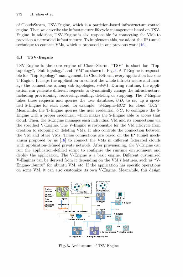
272 H. Zhou et al.
of CloudsStorm, TSV-Engine, which is a partition-based infrastructure controlengine. Then we describe the infrastructure lifecycle management based on TSV-Engine. In addition, TSV-Engine is also responsible for connecting the VMs toprovision a networked infrastructure. To implement this, we adopt the IP tunneltechnique to connect VMs, which is proposed in our previous work [16].
4.1 TSV-Engine
TSV-Engine is the core engine of CloudsStorm. “TSV” is short for “Top-topology”, “Sub-topology” and “VM” as shown in Fig. 3. A T-Engine is responsi-ble for “Top-topology” management. In CloudsStorm, every application has oneT-Engine. It helps the application to control the whole infrastructure and man-age the connections among sub-topologies, subNI. During runtime, the appli-cation can generate different requests to dynamically change the infrastructure,including provisioning, recovering, scaling, deleting or stopping. The T-Enginetakes these requests and queries the user database, UD, to set up a speci-fied S-Engine for each cloud, for example, “S-Engine-EC2” for cloud “EC2”.Meanwhile, the T-Engine queries the user credential, UC, to configure the S-Engine with a proper credential, which makes the S-Engine able to access thatcloud. Then, the S-Engine manages each individual VM and its connections viathe specified V-Engine. The V-Engine is responsible for the VM lifecycle fromcreation to stopping or deleting VMs. It also controls the connection betweenthe VM and other VMs. These connections are based on the IP tunnel mech-anism proposed by us [16] to connect the VMs in different federated cloudswith application-defined private network. After provisioning, the V-Engine canrun the application-defined script to configure the runtime environment anddeploy the application. The V-Engine is a basic engine. Different customizedV-Engines can be derived from it depending on the VM’s features, such as “V-Engine-ubuntu” for ubuntu VM, etc. If the application has specific operationson some VM, it can also customize its own V-Engine. Meanwhile, this design
Fig. 3. Architecture of TSV-Engine

CloudsStorm: An Application-Driven Framework 273
makes our framework very extensible. For example, in order to take Cloud Azureinto account, we therefore first derive “S-Engine-Azure” to manage Azure cloud.Afterwards, we add the credential and database information in “UserCredential”and “UserDatabase”. Then, the T-Engine can take the new cloud into accountwhen doing partitioning and manage the whole lifecycle of the resource fromthat cloud.
In addition, all the S-Engines and V-Engines are running in multi-thread. Itmeans that the T-Engine can start several S-Engines at the same time. If the sub-topologies managed by these S-Engines belong to different data centers, there willbe no contention among them. It is the same for V-Engine. In other words, TSV-Engine accelerates the controlling process. This engine has also been integratedin the software release of EU project, SWITCH [17], to be the fundamentalprovisioning engine.
4.2 Implementation of Control Mechanism
In order to control infrastructures, we define 5 statuses for the sub-topologyin CloudsStorm. These statuses are recorded in the infrastructure descriptionsshown in Fig. 1. Figure 4 is the status transition graph. It begins with the “Fresh”status, which means the infrastructure is in the design phase and the public IPsare not assigned. When the T-Engine controls the S-Engine to do provision-ing, the status of the sub-topology infrastructure can transit into two statuses,“Running” or “Failed”, depending on whether there are errors during provision-ing. If becoming “Running”, the public IPs of VMs in the running sub-topologymust have been assigned. Afterwards, if the control agent detects some run-ning sub-topology is not accessible or failed, the T-Engine marks its status as“Failed” and controls the corresponding S-Engine to identify the failed sub-topology. Meanwhile, all the sub-topologies which originally are connected withthis failed one should be detached. The failed sub-topology then can be recov-ered within another data center according to the recovery requests. “Stopped”status is circled with dashed line, because some clouds do not provide the stop-ping function. If the cloud doesn’t support this function, there is no “Stopped”status in its lifecycle. The reason for designing the status “Stopped” in the life-cycle is that the stopped VM is faster to bring up again than provisioning new
Fig. 4. Status transition of infrastructure lifecycle in CloudsStorm

274 H. Zhou et al.
one from “Fresh” when scaling up. Finally, “Deleted” is the terminated statusof the lifecycle. All the “Stopped” and “Running” infrastructures can be deletedto release resources.
5 Evaluation
In this section, we compare CloudsStorm with other related DevOps tools andevaluate it from two aspects, functionality and performance.
5.1 Functionality Evaluation
Table 1 shows the functionality comparison among different related tools andframeworks. We classify these DevOps tools into three categories. They areAPI-centric, infrastructure-centric and application-centric. The latter two bothbelong to the category of environment-centric. In this table, × and
√means sup-
ported and not supported respectively. − indicates partial support. For instance,some tools partially support auto-scaling and failure recovery, because somemanual work is still needed to actually trigger the process. Another case iswhere the auto-scaling refers to configuration scaling on pre-existing resources. Inthe programmability comparison, “Abstract description” indicates whether thetool allows the application to describe high level QoS constraints on the infras-tructure. For controllability comparison, “Multi-Mode” is explained in Sect. 4.2.“Decentralized” demonstrates the infrastructure management is in a decentral-ized way. If it is not, it means all the application developers’ infrastructures aremanaged by one administration, which requires everyone’s cloud credentials. If itis partial, it means an application developer can set up his own server for man-aging all his infrastructures instead for one application. Table 1 demonstratesCloudsStorm is application-driven and enhances the application’s programma-bility and controllability on its infrastructure.
5.2 Performance Evaluation
We conduct some experiments on actual clouds to evaluate CloudsStorm’s per-formance on auto-scaling and failure recovery. We also compare its performancewith some other related tools.
Auto-Scaling and Failure Recovery. These two are the key controllabilityof CloudsStorm. We design the experiment on ExoGENI to test the auto-scalingperformance. In this experiment, there are two sub-topologies in the beginning,subNI1 containing 1 VM and subNI2 containing 8 “XOMedium” VMs. EachVM in subNI2 is connected with the VM in subNI1 via a private network link.This is a typical “Master/Slave” distributed framework. subNI2 is defined asa scaling group. According to the scaling request, the infrastructure can scaleup to other data centers based on one or multiple copies of subNI2. At the

CloudsStorm: An Application-Driven Framework 275
Table
1.Funct
ionality
com
pari
son
am
ong
diff
eren
tD
evO
ps
tools
and
fram
ework
s

276 H. Zhou et al.
same time, all the network links between the scaled copies and subNI1 areconnected. These connections leverage private addresses, which can be definedbefore actual provisioning. Hence, the “Master” in subNI1 can always knowwhere are the scaled resources are. Figure 5 illustrates that we scale up the 8VMs of subNI2 accordingly at 1, 2, 3, 4, 8 and 16 times. Each scaled subNI2is provisioned in independent data centers simultaneously. Therefore, the flatdashed line is the ideal scaling performance in theory. However, the provisioningperformances of different data centers are not the same. This is demonstrated bythe varied dashed line, which is the average value of the maximum provisioningoverhead among the scaled subNI2. Moreover, the end-to-end connections needto be set up. The more copies of subNI2 requested, the more connections needto be configured. The solid line in the figure shows total cost. For each scale, weconduct 10 repeated experiments. The error bar denotes the standard deviation.It demonstrates that the scaling overhead does not grow at the same proportionas the number of VMs being created. Therefore, it is able to complete large-scale auto-scaling in a short time. In addition, most clouds have limitations onthe resource allocation. For instance, ExoGENI only allow one user to applya maximum of 10 VMs from one data center. The limitation for EC2 is 20.Nevertheless, with CloudsStorm, we can break through these limits to realizelarge-scale scaling by combining resources from different data centers and evenclouds.
Fig. 5. Auto-scaling performance Fig. 6. Failure recovery performance
Figure 6 shows the experimental result on failure recovery. In this experiment,there are still two sub-topologies in the beginning, subNI1 and subNI2. Each ofthem contains only one VM, n1 and n2. These two nodes are connected with theprivate network. Then we simulate the case where the data center of subNI2 isnot available. CloudsStorm recovers the same sub-topology from another datacenter or cloud. Finally, the private network is resumed. Hence, the applicationis not aware of this infrastructure modification. We get the detaching overheadfrom CloudsStorm, which is the time for subNI1 to disconnect the original link.It is illustrated by the bar covered with dots. On the other aspect, we continually

CloudsStorm: An Application-Driven Framework 277
test the private link from n1 of subNI1 to n2 of subNI2 and record the time fromlost connection to the time that the link is resumed. This is the total recoveryoverhead. We conduct this experiment on 3 clouds currently supported and pick6 data centers from them. In order to compare, n2 always has 2 cores and around8G memory with “Ubuntu 14.04”. Correspondingly, they are “t2.large” of EC2,“XOLarge” of ExoGENI and “mem medium” of EGI. The results show Exo-GENI has a relative higher recovery overhead and some of its data centers arenot stable. The performance of EC2 and EGI are close, however, most data cen-ters of EC2 are more stable. These information are important to decide where torecover to satisfy the application QoS, considering about the recovery overheadand data center geographic information.
Comparison. Finally, we conduct a set of experiments to compare CloudsStormwith other DevOps tools. We pick jclouds from API-centric tools. It is adoptedby a lot of environment-centric tools to be the basic provisioning engine, suchas CloudPick [4]. From environment-centric tools, we pick Nimbus team’s clou-dinit.d. Other tools like Juju and IM provide graphical interfaces, which makesit difficult to measure performance. Both of jclouds and cloudinti.d do not sup-port networked infrastructure. The ones which support networked infrastructurecan only be applied in private data centers, which CloudsStorm cannot have theaccess permission, like SAVI. We pick EC2 to do these experiments, becausethis is the most popular cloud provider and commonly supported by these tools.First, we compare the scaling performance. The scaling request is to add 5 more“t2.micro” VMs in EC2 California data center. However, jclouds and cloudinit.dcannot directly support auto-scaling behavior, we use them to provision 5 newVMs in California data center to simulate this scenario. For each operation,we repeated 10 times. Figure 7(a) illustrates the results. For jclouds, the provi-sioning process proceeds in sequence, hence, its scaling overhead is much morebigger than the other two. If only considering the scaling performance from“Fresh” (defined in Sect. 4.2) state, cloudinit.d and CloudsStorm have similarperformance, demonstrated by the bars covered with slashes. CloudsStorm is alittle bit stable than cloudinit.d. Moreover, EC2 supports stopping a instance.CloudsStorm can perform auto-scaling from “Stopped” status. It reduces theoverhead, shown by the bars covered with dots. It is worth to mention that wedo not consider deployment overhead in this experiment. Scaling from “Stopped”status can even omit the deployment. Through this way, CloudsStorm outper-forms cloudinit.d much better, reducing the scaling overhead by more than halfreferring to Fig. 7(b) and (c).
The second experiment is to compare the provisioning performance includingdeployments. All of these three allow users to define a script to deploy applica-tions immediately after provisioning. In this experiment, we choose Californiadata center to provision 5 “t2.micro” VMs and install tomcat on each of them.Each test is repeated 10 times. Figure 7(b) shows the results. With jclouds, theapplication are installed one by one, which costs plenty of time. For CloudsStorm,there is a V-Engine responsible for each individual VM to provision and deploy.

278 H. Zhou et al.
Fig. 7. Performance comparison
Therefore, it achieves the best performance according to the overhead and sta-bility. The last experiment is based on the second experiment considering aboutthe deployment dependency. In this experiment, 4 out of 5 VMs install tom-cat and the remaining one installs a mysql database. In this case, there is adependency when using jclouds and cloudinit.d, because they do not provisionnetworked infrastructure and use public addresses. Tomcat can only be deployedafter provisioning mysql VM to know the server address. Hence, jclouds needsto provision mysql VM first in its sequence. Cloudinit.d defines different lev-els to realize the dependency. In this scenario, the first level is the mysql VMand the second level contains four tomcat VMs. The difference for CloudsStormis that it can provision networked infrastructure. The nodes are connected withapplication-defined private network links. The mysql server address is pre-definedbefore actual provisioning. Therefore, all the deployments can proceed simulta-neously even with the dependency. Figure 7(c) demonstrates that the deploymentdependency makes smaller influence on CloudsStorm’s performance comparingto that on jclouds and cloudinit.d. We can reason out that if there are moredependencies, CloudsStorm has a greater advantage over others.
6 Discussion
There are plenty of application scenarios for CloudsStorm. To benefit from thenetworked infrastructure, a lot of programming models are easy to deploy, suchas Master/Slave (including docker cluster), Map/Reduce and workflow. Thesemodels are usually leveraged by big data processing. To benefit from the sufficientand efficient controllability, it is useful for IoT applications and sensor-cloud. Tobenefit from the application-driven design, we can bring the infrastructure intothe application incremental development phase. For example, testing the appli-cation with several VMs in the beginning and final release running on a large-scale infrastructure. Therefore, CloudsStorm narrows the DevOps gap and weare going to try to migrate more applications onto clouds through CloudsStormin the future work.

CloudsStorm: An Application-Driven Framework 279
Acknowledgment. This research has received funding from the European Union’sHorizon 2020 research and innovation program under grant agreements 643963(SWITCH project), 654182 (ENVRIPLUS project) and 676247 (VRE4EIC project).The research is also partially funded by the COMMIT project. The author, Huan Zhou,is also sponsored by China Scholarship Council.
References
1. Wettinger, J., et al.: Streamlining DevOps automation for Cloud applications usingTOSCA as standardized metamodel. FGCS 56, 317–332 (2016)
2. Keahey, K., Freeman, T.: Contextualization: providing one-click virtual clusters.In: IEEE Fourth International Conference on eScience 2008, pp. 301–308 (2008)
3. Caballer, M., de Alfonso, C., Molto, G., Romero, E., Blanquer, I., Garcıa, A.:Codecloud: a platform to enable execution of programming models on the clouds.J. Syst. Softw. 93, 187–198 (2014)
4. Dastjerdi, A.V., Garg, S.K., Rana, O.F., Buyya, R.: CloudPick: a framework forQoS-aware and ontology-based service deployment across clouds. Softw.: Pract.Exp. 45, 197–231 (2015)
5. Diaz-Montes, J., AbdelBaky, M., Zou, M., Parashar, M.: CometCloud: enablingsoftware-defined federations for end-to-end application workflows. IEEE InternetComput. 19(1), 69–73 (2015)
6. Jeferry, K., Kousiouris, G., Kyriazis, D., Altmann, J., Ciuffoletti, A., Maglogiannis,I., Nesi, P., Suzic, B., Zhao, Z.: Challenges emerging from future cloud applicationscenarios. Procedia Comput. Sci. 68, 227–237 (2015)
7. Marshall, P., Tufo, H.M., Keahey, K., La Bissoniere, D., Woitaszek, M.: Archi-tecting a large-scale elastic environment-recontextualization and adaptive cloudservices for scientific computing. In: ICSOFT (2012)
8. Caballer, M., Blanquer, I., Molto, G., de Alfonso, C.: Dynamic management ofvirtual infrastructures. J. Grid Comput. 13(1), 53–70 (2015)
9. Zhao, Z., Grosso, P., Van der Ham, J., Koning, R., De Laat, C.: An agent basednetwork resource planner for workflow applications. Multiagent Grid Syst. 7(6),187–202 (2011)
10. Wang, J., Taal, A., Martin, P., Hu, Y., Zhou, H., Pang, J., de Laat, C., Zhao,Z.: Planning virtual infrastructures for time critical applications with multipledeadline constraints. Future Gener. Comput. Syst. 75, 365–375 (2017)
11. Hu, Y., Wang, J., Zhou, H., Martin, P., Taal, A., de Laat, C., Zhao, Z.: Deadline-aware deployment for time critical applications in clouds. In: Rivera, F.F., Pena,T.F., Cabaleiro, J.C. (eds.) Euro-Par 2017. LNCS, vol. 10417, pp. 345–357.Springer, Cham (2017). https://doi.org/10.1007/978-3-319-64203-1 25
12. Ouyang, X., Garraghan, P., Primas, B., McKee, D., Townend, P., Xu, J.: Adaptivespeculation for efficient internetware application execution in clouds. ACM Trans.Internet Technol. (TOIT) 18(2), 15 (2018)
13. Zhao, Z., Van Albada, D., Sloot, P.: Agent-based flow control for HLA components.Simulation 81(7), 487–501 (2005)
14. Baldin, I., et al.: ExoGENI: a multi-domain infrastructure-as-a-service testbed. In:McGeer, R., Berman, M., Elliott, C., Ricci, R. (eds.) The GENI Book, pp. 279–315.Springer, Cham (2016). https://doi.org/10.1007/978-3-319-33769-2 13

280 H. Zhou et al.
15. Kang, J.-M., Lin, T., Bannazadeh, H., Leon-Garcia, A.: Software-defined infras-tructure and the SAVI testbed. In: Leung, V.C.M., Chen, M., Wan, J., Zhang,Y. (eds.) TridentCom 2014. LNICST, vol. 137, pp. 3–13. Springer, Cham (2014).https://doi.org/10.1007/978-3-319-13326-3 1
16. Zhou, H., Wang, J., Hu, Y., Su, J., Martin, P., de Laat, C., Zhao, Z.: Fast resourceco-provisioning for time critical applications based on networked infrastructures.In: IEEE International Conference on Cloud Computing, pp. 802–805 (2016)
17. Zhao, Z., Taal, A., Jones, A., Taylor, I., Stankovski, V., Vega, I.G., Hidalgo,F.J., Suciu, G., Ulisses, A., Ferreira, P.: A software workbench for interactive,time critical and highly self-adaptive cloud applications (SWITCH). In: 2015 15thIEEE/ACM International Symposium on Cluster, Cloud and Grid Computing(CCGrid), pp. 1181–1184. IEEE (2015)

A RESTful E-Governance ApplicationFramework for People Identity
Verification in Cloud
Ahmedur Rahman Shovon, Shanto Roy, Tanusree Sharma,and Md Whaiduzzaman(B)
Institute of Information Technology, Jahangirnagar University, Dhaka, [email protected], [email protected], [email protected],
Abstract. An effective application framework design for e-governanceis definitely a challenging task. The majority of the prior research hasfocused on designing e-governance architecture where people identity ver-ification takes long time using manual verification system. We develop anefficient application framework that verifies peoples identity. It providescloud based REST API using deep learning based recognition approachand stores face meta data in neural networks for rapid facial recognition.After each successful identity verification, we store the facial data in theneural network if there is a match between 80–95%. This decreases theerror rate in each iteration and enhance the network. Finally, our systemis compared with the existing system on the basis of CPU utilization,error rate and cost metrics to show the novelty of this framework. Weimplement and evaluate our proposed framework which allows any orga-nization and institute to verify people identity in a reliable and securemanner.
Keywords: E-Governance · Cloud computing · RESTful APIID verification
1 Introduction
E-governance applications are based on Government to Government (G2G), Gov-ernment to Business (G2B), Government to Citizens (G2C) and Government toEnterprise (G2E) [1]. It is nothing but a service that act as a medium of exchangeof information, transactions and services. Cloud Computing is the delivery ofcomputing services servers, storage, databases, networking, software, analyticsand more over the Internet.
A number of issues have risen in e-governance application. The lack of appro-priate framework, content development, citizen access are the main problems.Every government needs to record the data of its citizens including national ID(NID) information and photo which are not updated regularly. In the mean timec© Springer International Publishing AG, part of Springer Nature 2018M. Luo and L.-J. Zhang (Eds.): CLOUD 2018, LNCS 10967, pp. 281–294, 2018.https://doi.org/10.1007/978-3-319-94295-7_19

282 A. R. Shovon et al.
a person’s look changes with his age. Thus verification can be problematic in thatcase. Here, updating photo is necessary which might be costly and requires morespace that remains idle mostly. Again large amount of data can make chaos andredundancy. For that an effective E-Governance system should be cost effective,reliable and easy to maintain. Unfortunately,current technologies are not enoughto meet the overall requirements of E-Governance [1].
To overcome the scenario, Cloud technology or mobile computing [2] is thesolution to the problems. E-governance is facing failure in meeting require-ments of public services, high IT budgets compared to low utilization of existingresources, poor security mechanisms, costly operations and maintenance (O &M) etc. [3]. Hence cloud based E-Governance application framework providesmany benefits in particular to government. It provides a comparatively betterplatform for efficient deployment of E-governance System [1] than the traditionalmanual processes.
Fig. 1. Block diagram of the proposed system
In this paper, we implemented a smart approach that the government cankeep only the vector co-ordination information in cloud for further verification.By adding images of a unique face and updating it with AWS AI approachesdecrease the error rate of people identity verification. The feature of deep learn-ing based image recognition technique make the system efficient for authorizedaccess. The increase of facial data of the citizens will open the door of futurestudy. Our system provides better CPU utilization, scope for migration to newtechnologies.Here, we used police verification data which eliminate manual ver-ification process and reduce the delay. Moreover, REST approach confirms theinstant response from verification framework that can be integrated to any autho-rized application. Overall, the primary contributions of this work are a people

A RESTful E-Governance Application Framework 283
verification framework, utilization of cloud for E-Governance application, REST-ful approach for better and secure service provision. For better understanding,the block diagram of the proposed system is showed on Fig. 1.
The remainder of the paper is organized as follows. Section 2 describes dif-ferent E-governance system proposed by several researchers. Section 3 describesour proposed methodology. Section 4 presents the architecture of the framework,Sect. 5 shows the results. Finally, Sect. 6 presents the conclusion and future workof this study.
2 Related Work and Motivation
In this section, we discuss several existing E-governance system and also describeour motivation for this study.
2.1 Related Work
Several researchers have developed and surveyed some system for E-governance.For example Witarsyah, et al. in [4] studied on adding some important variables:trust, information quality, system quality of e-government adoption in improvingservice to the citizen. In [5] Rao and Krishna proposed a system comparing withexisting system on the basis of browsing performance, response time, and securityto show that novelty nature of the software architecture to support e-governanceof India on highly distributed evaluation environment. Hence, information qual-ity and data scaling are ignored here. In [6] Zissis and Lekkas proposed a highlevel electronic governance and electronic voting solution, supported by cloudcomputing architecture and cryptographic technologies. It is quite clear fromthis paper that there is a large scope for further research.
Zhang and Chen in [7] introduced a new concept of C-government that uti-lizes cloud computing in e-governance. Authors designed the architecture anddiscussed about the implementation and deployment of the c-government system.The paper also explained how citizen engagement is maximized with enhancedcollaboration towards government productivity and service delivery. Hashemiet al. In [8], authors discussed about the benefits of using cloud computationin e-governance including improvement and optimization providing public ser-vices, governments enhanced ability to interact and collaborate, achieving trans-parency and accountability as well as overall improvement of the relationshipbetween the government and its citizens etc. How developed countries like Sin-gapore, USA and UK are adapting to the cloud technology is also mentionedhere. In [9] Cellary and Strykowski researched on two levels of aggregation: orga-nizational units and functional modules. Some mentionable advantages of cloudare: dynamic load of resources, proper maintenance and administration, higherperformance etc. Authors also claims that REST based web technology is gaininga lot of attractions.
Face verification across ages has importances in some potential applicationssuch as passport photo verification, image retrieval and post processing, surveil-lance etc. [10]. As human faces change in course of time and still the face image

284 A. R. Shovon et al.
may need some verification. Photo identification means the matching accuracy inpercentage using 3D modeling [11], discriminative methods [10], feature extrac-tion and modeling through deep learning etc [12–14].
In [15] Christensen et al. implies to the integration of REST-based web serviceand cloud computing in order to create futuristic web and mobile applicationsalong with optimization and security. As REST architecture ensures the datasecurity as well as maintains a secure communication [16]; that is the reasonbehind choosing this technology in our work.
2.2 Motivation
From our observation, as discussed in Subsection A of Sect. 2 we can come to aconclusion that we needed to develop an framework that includes digitization,proper citizen access, increase facial data of each citizen, lowest cost, lower errorrate of face recognition. To get the best performance of E-governance systemwe need to focus on this trade-off. Therefore, in our proposed policy we take amore holistic approach by considering a RESTful API can be accessed from anydevice that is connected with internet.
3 Methodology
We designed the architecture to verify people identity and personal informationin G-cloud using the secure RESTful API. The process starts with searchinginformation in the database using NID; matches the facial vector data with thestored data mapped with the NID. The system flowchart and algorithm areshown in Fig. 2 and Algorithm 1 accordingly.
4 Architecture of the Framework
Our proposed system developed an E-Governance application framework whichincludes hardware and software requirements and it uses cloud based artificialneural network.
4.1 Structural Description
The proposed framework uses the Amazon Web Service (AWS) for all operations.The REST API is hosted in EC2 instance and can be accessible via API callsfrom any other systems. The REST API is built using Python Flask Frameworkand it abides by the prescribed standard of HTTP status codes. JSON WebToken (JWT) which is a JSON based open standard for creating access tokensis used to authenticate the API calls. For storing the newly compared faces, theframework uses Rekognition and Elastic Load Balancer (ELB) from AmazonWeb Services. For storing the public people data it utilizes the functionalities ofSQLAlchemy, Python SQL Toolkit and Object Relational Mapper (ORM) that

A RESTful E-Governance Application Framework 285
API Call
Search People Informa on and Image using NID
NID found?
Return Error: Invalid NID
Get data associated with NID
Return Error: Invalid data
Data matched AND max
face similarity > 80%?
Return Error: Police clearance
failed
Check Police Record
Y N
N
Y
Police Record: Clean ?
max face similarity < 95%?
Return Success: Person data
Add face in Collec on
Valid Token? Return Error: Invalid Token
Y
N
N
Y
Y
N
Fig. 2. System flowchart
provides full power and flexibility of SQL. The ORM is connected with MySQLdatabase for handling the queries.
In this scenario, there are 4 subnets in the (Virtual Private Cloud) VPC.Three of them are private and one public. In each subnets the proposed frame-work used Application server, Database server, API Server which are in theprivate subnets. In the public subnet there is a bastion host which is used bythe developer to SSH on each server in the VPC.
4.2 Functionalities
There are two Classic Load Balancers are used in this application. One is publicfacing load balancer in which users can connect to its port 80 and internallyit connects to the web application. Other is internal load balancer by whichthe application communicates with the API. Each load balancer there is an

286 A. R. Shovon et al.
Fig. 3. System architecture
auto scaling group which scales the application and API servers. Mobile userscan directly hit the API server through the public facing elastic load balancer(Fig. 3).
4.3 Requirement Analysis
The necessary software and hardware tools needed to complete this work aredescribed in Tables 1 and 2 accordingly.
4.4 Security
The instances in the public subnet can send outbound traffic directly to the Inter-net, whereas the instances in the private subnet can’t. Instead, the instances inthe private subnet can access the Internet by using a network address trans-lation (NAT) gateway that resides in the public subnet. The database serverscan connect to the Internet for software updates using the NAT gateway, butthe Internet cannot establish connections to the database servers. Web appli-cation, API and database cannot accessible from the Internet. Each subnet hasits own security groups. In the security groups inbound and outbound rules areconfigured for the security and application needs.
5 Implementation and Results
We used Machine Learning approaches in E- governance system and developeda framework with RESTful API for citizen access.
A RESTful E-Governance Application Framework 287
5.1 Implementation Environment
The deployment procedure of our proposed framework in started with creatingnew VPC which includes three public and one private subnet. Later we create anInternet gateway and a NAT gateway from which NAT gateway is placed in pub-lic subnet and associate an EIP to it Then finally create route by adding IGW tothe public subnet and NAT Gateway to the private subnet.After that we initial-ize security group for each subnet for security purpose and create dashboard-secfor dashboard subnet, db-sec for db-subnet, api-sec for api segment and jump secfor jump subnet. Then we create an EC2 instance for dashboard application. Wedeployed the code base and create an Internet facing classic load balancer.Aftercreating a launch configuration with dashboard application, we also create autoscaling group and add load balancer that previously created. We add the scal-ing policy on CPU utilization which scales the servers and send alerts throughemails.
We designed four tables for our database named authenticated organization,people, aws face, and police record. The fields needed for the tables are listedin Table 3. People table has relation with aws face and police record using thenational id field. To create JSON Web Token for API call authenticity, a com-bination of organization’s id, email address and password will be used.
5.2 Performance Evaluation
Primarily the neural network contains one picture per person mapped to thepersons NID. For this reason, falsification of face recognition is occurred in somecases. We used the face recognition technology (FERET) database [17] whichis a dataset used for facial recognition system evaluation to measure the errorrate. We mapped one individual photo with one national id. Then we tested thesystem using same individual’s other photos available in the FERET database.
We calculate the error rate of the framework by measuring number of falseresults returned by the API. At first, the neural network has only one image perperson. We mark this stage as single image stage. In each verification request ifthere is 80–95 % similarity then the framework adds the new image to neuralnetwork. By using this machine learning approach provided by AWS, it becomeseasy and efficient to verify people by the increasing number of iterations. As thenumber of iteration is increases, the error rate is decreases. Even for this deeplearning approach, this image data can be used further for video verification.
Error rate in this single image per person scenario is 1.60%. After this iter-ation, each searched persons have two facial data (on average) available. Theerror rate in this scenario is 1.13%. In third iteration, there are three facial data(on average) is available for each person. The error rate in this step is 0.27%.The improvement of each iteration is shown in Fig. 4.
5.3 Scalability Evaluation
To evaluate the scalability of our framework we chose CPU utilization as pri-mary metric. The auto load testing script which is developed is used to generate

288 A. R. Shovon et al.
Fig. 4. Performance chart in each verification iteration
artificial hit on the API endpoints. The CPU utilization of EC2 instances ofPeople Identity Verification API is shown in Fig. 5. The Y axis reflects the CPUutilization and is measured in percentage which go up by 5 percent at each level.The X axis represents time frame. The instances are configured to add multipleinstances instantly in case of high CPU utilization.
Fig. 5. CPU utilization of People Identity Verification API
Furthermore, we generate excessive hit on the API endpoints using test scriptand exceeds the maximum limit of CPU power. Our system is configured togenerate alert for low and excessive CPU utilization within a time range and addadditional computing resources as needed. The additional resources are detachedfrom the system when the CPU utilization becomes normal. Figure 6 shows ascenario of live monitoring the instances.
5.4 Cost Evaluation
For any application framework, cost assumption is important to evaluate theefficiency and usability. We deployed our application in Amazon Web Services

A RESTful E-Governance Application Framework 289
Fig. 6. Auto scaling alert monitoring
(AWS) which offers a pay-as-you-go approach. With AWS the application needsto pay only for the individual services it needs, for as long as it uses them. Itrequires to pay for the services the application framework consumes, and onceit stop using them, there are no additional costs or termination fees. If we usednon cloud hosting for our application framework neither it would not scalablenor efficient. The charges of various services utilization are shown in Fig. 7. Thisfigure proves that costing is reliable and efficient for this application framework.
Fig. 7. People Identity Verification API costing graph
6 Discussion
In this section, we discuss the advantages, application areas, scopes and limita-tions of our framework.

290 A. R. Shovon et al.
Algorithm 1: Algorithm for people verificationAPI call;if TOKEN in Request = True then
if V alidityTOKEN = True thenif NID, personal information & image in Request then
if NIDfound = True thenif personal information & image matches with database then
Get Face List from Database;Set MaxScore = 0 ;foreach Face in Face List do
Calculate similarity score;Set MaxScore = max(score,max score);
endif MaxScore > 80 then
if MaxScore < 95 thenStore image in Collection;
endGet RecordsPolice ;if Clearence = True then
Return: Verification Success with all data;endelse
Return Error with case record details;end
endelse
Return Error: Image match failed;end
endelse
Return V erified = True;end
endelse
Return Error: NID not found;end
endelse
Return Error: Missing mandatory fields;end
endelse
Return: TOKEN not valid;end
endelse
Return: TOKEN not found;end
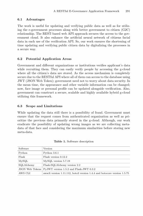
A RESTful E-Governance Application Framework 291
6.1 Advantages
The work is useful for updating and verifying public data as well as for utiliz-ing the e-government processes along with better government to citizen (G2C)relationship. The REST-based web API approach secures the access to the gov-ernment cloud. It also enhance the artificial neural network of citizens facialdata in each use of the verification API. So, our work ensures the shortening oftime updating and verifying public citizen data by digitalizing the processes ina secure way.
6.2 Potential Application Areas
Government and different organizations or institutions verifies applicant’s datawhile recruiting them. They can easily verify people by accessing the g-cloudwhere all the citizen’s data are stored. As the access mechanism is completelysecure due to the RESTful API where all of them can access to the database usingJWT (JSON Web Token); government need not to worry about data security. Inthe mean time, the appearance and other variable information can be changed;now, face image or personal profile can be updated alongside verification. Also,government can construct a secure, scalable and highly available hybrid g-cloudutilizing this framework.
6.3 Scope and Limitations
While updating the data still there is a possibility of fraud. Government mustensure that the request comes from authenticated organization as well as pri-oritize the previous data primarily stored in the g-cloud. Although, our workeradicate the possibility of updating wrong images as we are collecting meta-data of that face and considering the maximum similarities before storing newmeta-data.
Table 1. Software description
Software Version
Python Python 3.6.1
Flask Flask version 0.12.2
MySQL MySQL version 5.7.19
SQLAlchemy Flask-SQLAlchemy version 2.2
JSON Web Tokens PyJWT version 1.5.2 and Flask-JWT 0.3.2
AWS CLI awscli version 1.11.112, boto3 version 1.4.4 and botocore version 1.5.75

292 A. R. Shovon et al.
Table 2. Hardware description
Hardware Description
VPC A VPC with three private subnets and one public subnet iscreated to host the whole application
Bastion node Bastion server is needed to access the others servers as itincludes the public inbound rules and private outbound rules.We have chosen m1-large EC2 instance for this node
API and APIdashboard node
The main Flask API and its dashboard are deployed in EC2instances. For both operation, we have chosen m1-large instancewhich include Auto scaling groups. The AWS services likeRekognition, AMI, AWSCLI are performed from these nodes
Database node The database is hosted in this node. It is also a m1-large EC2instance and has only private access from the other nodes
Load balancers Two Elastic Load Balancers ensure to handle the inbound trafficfor both API access and API dashboard access
Security groups Proper security groups are created for handing the inbound andoutbound traffic in each node and services to restrictunauthenticated access of the application
Table 3. Fields of database
Table name Fields
authenticated organization organization id (PK), organization email address,organization password, organization name,organization address, organization phone number,organization email address, organization registration id,organization registration address, organization details
people national id (PK), full name, father name, mother name,date of birth, gender, birth district, permanent address,present address, email address, phone number, blood group,nationality, religion, marital status, spouse name, tin number,passport number, driver license number, photo url,created timestamp, updated timestamp
aws face face id (PK), face created time, face url, national id (FK)
police record case id (PK), case status, case description, case location,case outcome, case created time, case updated time,case complainer national id (FK), case investigator national id(FK), case defendant national id (FK)
7 Conclusion
We developed an efficient approach towards the verification of people throughsecurely accessing the public database supervised by government. We utilized thebenefits of RESTful approach for ensuring security. All governments can utilizethe hybrid architecture to ease the entire process thereby. Overall, this systemprovides public services in a faster way eradicating long time-wasting analog pro-cesses with its’ features of digitization, citizen access, developed content. Here,

A RESTful E-Governance Application Framework 293
the deep learning based people verification approach improves the performancerapidly in each iteration. It is proved by the improvement of identity verificationby 29.38% and 76.11% in first and second iteration. Again application pay onlyfor the individual services it needs by using AWS which ultimately reduce thecost. We are storing the meta-data of every updated face image of people in aneural network. Increasing number of stored meta-data opens door to track allthe people in a country or within a particular region boundary. The frameworkcan be integrated with any authorized application to verify people’s identitywith ease.
References
1. Smitha, K.K., Thomas, T., Chitharanjan, K.: Cloud based E-Governance system:a survey. Procedia Eng. 38, 3816–3823 (2012)
2. Whaiduzzaman, Md., Naveed, A., Gani, A.: MobiCoRE: mobile device basedcloudlet resource enhancement for optimal task response. In: IEEE Transactionson Services Computing (2016)
3. Liang, J.: Government cloud: enhancing efficiency of E-Government and providingbetter public services. In: 2012 International Joint Conference on Service sciences(IJCSS), pp. 261–265. IEEE (2012)
4. Witarsyah, D., Sjafrizal, T., Fudzee, M.D., Farhan, M., Salamat, M.A.: The criticalfactors affecting E-Government adoption in Indonesia: a conceptual framework. Int.J. Adv. Sci. Eng. Inf. Technol. 7(1), 160–167 (2017)
5. Rao, M.N., Krishna, S.R.: Efficient and ubiquitous software architecture of E-Governance for Indian Administrative Services. Int. J. Adv. Res. Comput. Sci.4(11), 66–74 (2013)
6. Zissis, D., Lekkas, D.: Securing E-Government and E-Voting with an open cloudcomputing architecture. Gov. Inf. Q. 28(2), 239–251 (2011)
7. Zhang, W.J., Chen, Q.: From E-Government to C-Government via cloud comput-ing. In: 2010 International Conference on E-Business and E-Government (ICEE),pp. 679–682. IEEE (2010)
8. Hashemi, S., Monfaredi, K., Masdari, M.: Using cloud computing for E-Government: challenges and benefits. Int. J. Comput. Inf. Syst. Control Eng. 7(9),596–603 (2013)
9. Cellary, W., Strykowski, S.: E-Government based on cloud computing and service-oriented architecture. In: Proceedings of the 3rd International Conference on The-ory and Practice of Electronic Governance, pp. 5–10. ACM (2009)
10. Ling, H., Soatto, S., Ramanathan, N., Jacobs, D.W.: A study of face recognitionas people age. In: 2007 IEEE 11th International Conference on Computer Vision,ICCV 2007, pp. 1–8. IEEE (2007)
11. Park, U., Tong, Y., Jain, A.K.: Age-invariant face recognition. IEEE Trans. PatternAnal. Mach. Intell. 32(5), 947–954 (2010)
12. Ling, H., Soatto, S., Ramanathan, N., Jacobs, D.W.: Face verification across ageprogression using discriminative methods. IEEE Trans. Inf. Forensics Secur. 5(1),82–91 (2010)
13. Sun, Y., Wang, X., Tang, X.: Deep learning face representation from predicting10,000 classes. In: Proceedings of the IEEE Conference on Computer Vision andPattern Recognition, pp. 1891–1898 (2014)

294 A. R. Shovon et al.
14. Taigman, Y., Yang, M., Ranzato, M.A., Wolf, L.: Deepface: closing the gap tohuman-level performance in face verification. In: Proceedings of the IEEE Confer-ence on Computer Vision and Pattern Recognition, pp. 1701–1708 (2014)
15. Christensen, J.H.: Using RESTful web-services and cloud computing to createnext generation mobile applications. In: Proceedings of the 24th ACM SIGPLANConference Companion on Object Oriented Programming Systems Languages andApplications, pp. 627–634. ACM (2009)
16. Adamczyk, P., Smith, P.H., Johnson, R.E., Hafiz, M.: Rest and web services: intheory and in practice. In: REST: From Research to Practice, pp. 35–57. Springer,New York (2011). https://doi.org/10.1007/978-1-4419-8303-9 2
17. Color FERET Database. https://www.nist.gov/itl/iad/image-group/color-feret-database. Accessed 03 Oct 2017
A Novel Anomaly Detection AlgorithmBased on Trident Tree
Chunkai Zhang1(B), Ao Yin1, Yepeng Deng1, Panbo Tian1, Xuan Wang1,and Lifeng Dong2
1 Department of Computer Science and Technology, Harbin Institute of Technology,Shenzhen, China
[email protected], [email protected], [email protected], panbo [email protected],[email protected]
2 Department of Physics, Hamline University, 1536 Hewitt Avenue,
St. Paul, MN 55104, USA
Abstract. In this paper, we propose a novel anomaly detection algo-rithm, named T-Forest, which is implemented by multiple trident trees(T-trees). Each T-tree is constructed recursively by isolating the dataoutside of 3 sigma into the left and right subtree and isolating the oth-ers into the middle subtree, and each node in a T-tree records the sizeof datasets that falls on this node, so that each T-tree can be used asa local density estimator for data points. The density value for eachinstance is the average of all trees evaluation instance densities, and itcan be used as the anomaly score of the instance. Since each T-tree isconstructed according to 3 sigma principle, each tree in TB-Forest canobtain good anomaly detection results without a large tree height. Com-pared with some state-of-the-art methods, our algorithm performs wellin AUC value, and needs linear time complexity and space complexity.The experimental results show that our approach can not only effec-tively detect anomaly points, but also tend to converge within a certainparameters range.
Keywords: Anomaly detection · Isolation · Forest · 3 sigmaGaussian
1 Introduction
Anomaly points are the data points that deviate from most data and do notobey the distribution of most data points [1–3]. Anomaly detection has been awidely researched problem in several application domains such as system healthmanagement, intrusion detection, healthy-care, bio-informatics, fraud detection,and mechanical fault detection. For these applications, anomaly detection asan unsupervised learning task is very important. The significance of anomalydetection is due to the fact that anomaly data can be translated into importantoperational information in various application domains. For example, with the
c© Springer International Publishing AG, part of Springer Nature 2018M. Luo and L.-J. Zhang (Eds.): CLOUD 2018, LNCS 10967, pp. 295–306, 2018.https://doi.org/10.1007/978-3-319-94295-7_20

296 C. Zhang et al.
development of cloud computing [4–7], it is very important to detect abnormaltraffic in the cloud in a timely manner. And with the development of the cloudstorage [8,9], timely detection of abnormal disk reads and writes in cloud storagecan greatly reduce the potential risk of cloud storage.
Many unsupervised anomaly detection approaches, including classification-based [10,11], clustering-based [12,13], density-based [14–17], and angle-baed[18], calculate the distance between data points to determine their similarity,and then determine whether the data points are abnormal. There are manyways to calculate the distance, such as Euclidean distance, DTW, and so on. Byanalyzing the characteristics of these distance calculation formulas, we can getthat the result can be easily affected by the data values and the number of dataattributes. And many of the above algorithms are constrained to low dimensionaldata and small data size due to the high computational complexity of its originalalgorithm. In order to solving the above problems, Liu et.al proposed a differentapproach that detects anomalies by isolating instances, without relying on anydistance or density measure [19,20]. In this approach, since the attribute andthe split value of each node in the isolation tree are randomly selected, the builtisolation tree can also be called a completely random tree. Consequently, thereis often a certain degree of randomness in the anomaly detection results by usingsuch a model.
In response to these challenges, we propose a novel anomaly detection algo-rithm on the basis of isolation-forest [19]. The key insight of our proposed algo-rithm is a fast and accurate local density estimator implemented by multiple tri-dent trees(T-trees), called T-Forest. The proposed approach can isolate anomalydata faster and more accurately. To achieve this, we extend the binary tree struc-ture of the original isolation tree to the structure of the trident tree. And insteadof selecting the split value randomly, we take advantage of sigma principle toselect two split values at a time to split the inconsistent attribute data as soonas possible. In this paper, we will show that trident trees can effectively isolateanomaly points.
The main contributions of this paper are summarized as follows:
– We propose a novel anomaly detection algorithm, called TB-Forest. Datapoints which have short average path on the T-tree, may be seen as anomalypoints.
– We propose a local density assessment method, which is used to estimate theanomaly degree of data points. We perform many experiments on benchmarkdataSets. The experiment results show that our proposed approaches outper-forms the competing methods on most of the benchmark dataSets in AUCscore.
The remainder of this paper is organized as follows. In Sect. 1, we review therelated work. In Sect. 2, we present the proposed anomaly detection algorithm. InSect. 3, we perform some empirical experiments to demonstrate the effectivenessof our algorithm. Lastly, the conclusion will be shown in Sect. 4.

A Novel Anomaly Detection Algorithm Based on Trident Tree 297
2 Anomaly Detection by Our Method
In this section, we will show the detailed steps of our proposed detection algo-rithm. We first show some definitions used in this paper. Then we present theimplementation details. Table 1 summarizes the symbols used in this paper.
2.1 Definitions
In this section, we will present the definition of T-tree and introduce theattributes of each node in a T-tree. And we definite the formula for calculatingthe anomaly score.
Table 1. Symbols and descriptions
Symbols Description
N Number of instances in a dataset
x An instance
X A dataset of N instances
Q A set of attributes
q An attribute
uq The mean of the attribute q
σq The standard deviation of the attribute q
T A tree
Tr A right tree of a node τ
Tl A left tree of a node τ
Tm A middle tree of a node τ
pl The split value between left tree and middle tree, uq − 3σq
pr The split value between middle tree and left tree, uq + 3σq
t Number of trees
ψ Sample ratio
den(x) The number of contained instances of the external node that x belongs to
hlim Height limit
slim Size limit in training a tree
Definition 1. T-tree: Let T denote a T-tree and τ be a node in this T-tree.It is either an external-node with no child, or an internal-node with a set andexactly three child trees(Tl,Tm,Tr). Each node in a T-tree contains the followingelements:(1) variables pl and pr, which are used to divide data points into Tl, Tm,and Tr subtree; (2) variable size, which is used to record the instances numberlocated in this node; (3) three node pointers, which are used to the left subtree,the right subtree, and the middle subtree.
Given a sample of data X={x1, x2, ..., xn} of n instances, in which each xi
has d attributes, to build a trident tree(T-tree). Figure 1 is used as an example

298 C. Zhang et al.
to illustrate the structure of a T-tree. We recursively divide X by randomlyselecting an attribute q and calculating the left split value pl and the right splitvalue pr, until either: (1) the tree height reaches limit, hlim, (2) the numberof instances at a node τ is less than the size limit, slim or (3) all points of theselected attribute have the same value in X. An T-tree has the property as BST,that is, the value of an attribute in left child tree is less than the middle side andthe middle size is less than the right side. Assuming all instances are distinct,the number of instances in left child tree is equal to the number in the right side.Since each leaf node in the MB-Tree contains no fewer than one instance andeach internal node contains exactly three children, the total number of nodes ina T-tree is less than 3N
2 − 1. Hence, an MB-Tree is only linear storage overhead.
Fig. 1. This figure is used as an example to illustrate the structure of a T-tree andshow the process of the division. Round nodes represent internal nodes, and squarenodes represent external nodes.
In this paper, calculating a score for each data point that reflects the anomalydegree of each data point. Since all instances in the dataSets fall on differentexternal nodes after being divided several times according to different attributevalues, each node in a T-tree forms a local subspace and instances located oneach node have similar data characteristics. Instances on each node become K-nearest-neighbors to each other. Hence, we calculate the local density of theinstance by counting the number of instances in each node where the instancefalls, to determine the anomaly degree of the instance.
Anomaly Score: The anomaly score of each point x is measured by the averagelocal density, den(x). den(x) denotes the number of instances contained in theterminational node of x. Since we have adopted the idea of ensemble learningand the number of instances used to train each T-tree may be different, we needto normalise the value den(x) in order to calculate the final anomaly score byusing all results in the TB-Forest. Therefore, the anomaly score of an instancecan be defined as follows:

A Novel Anomaly Detection Algorithm Based on Trident Tree 299
score(x) =1t
t∑
i=1
deni(x)Ni
(1)
where deni(x) is the local density in a T-tree and Ni is the instances numberin T-treei. Because of the characteristics “less and different” of anomaly points,the value of score(x) will be less than the normal points. Therefore, the smallerthe value of score(x), the more abnormal it is. In other words, the closer ofthe value of score(x) is to 0, the more likely the corresponding instance is ananomaly point.
2.2 Training for T-Forest
In this section, we will introduce the concrete steps of building a T-Forest, whichis composed of many T-trees. Each T-tree is built on the dataset sampled byusing the variable bagging technique.
Building a T-tree: A T-tree can be constructed by recursively dividing thetraining datasets until the tree reaches height limit or the instances number isless than the size limit. During the construction of each node of a T-tree, anattribute will be randomly selected from the attributes of the datasets as thesplitting attribute. And these two splitting values, pl and pr, will be obtainedby calculating the mean value and the standard derivation of this attribute, andthen are used to divide the training datasets. The concrete steps to build a T-tree are described in Algorithm 1. The time complexity of this algorithm is onlyO(log3(N)), and the space complexity is liner O(N).
Building a T-Forest: There are three parameters that need to be set manuallyto the TB-Forest. They are the height limit of a T-tree hlim, the size limit ofeach node slim, and the tree number t. There is also a variable, sample ratio ψ,which is generated uniformly from the range between 0.2 and 0.8. This parametermay be different in each T-tree, so it can increase the diversity of samples ineach T-tree. The changes of these parameters will affect the evaluation effect.For example, many trees or a high T-tree can increase the accuracy of the result.However, after increasing to a certain value, the result will tend to converge. Ifthese two parameters are set too large, it not only did not improve the detectionperformance, but increase the model’s runtime and memory consumption. Thesize limit is always set to 15, because if the number of samples is less than 15, thecriteria 3 sigma will no longer apply. The concrete steps of TB-Forest algorithmare described as Algorithm 2. The time complexity of building a TB-Forest isO(t ∗ ψ ∗ log3(N)). The space complexity of building a TB-Forest O(t ∗ ψ ∗ N).
2.3 Evaluation Stage
In this evaluation stage, an anomaly score of instance x can be estimated bythe average local density E(den(x)). den(x) can be calculated by Algorithm3.After getting all den(x) of instance x by TB-Forest, we can use the formula

300 C. Zhang et al.
Algorithm 1: Building a T-tree(Data, cur, hlim, slim)Input: A dataSet Data, a current height cur, a height limit hlim, a size limit
slim.Output: A T-tree
1 if |Data| ≤ slim and cur ≥ hlim then2 return node(size=|Data|,exteral=TRUE);3 end4 Randomly select an attribute q ∈ Q.5 Calculate the mean value, uq, of the attribute q.6 Calculate the standard derivation, σ, of the attribute q.7 left-split ← uq − 3σ8 right-split ← uq + 3σ9 Datal ← data-filter(Data, x ≤ left-split)
10 Datam ← data-filter(Data, x >left-split and x <right-split)11 Datar ← data-filter(Data, x ≥ right-split)12 Left-Tree ← Building-Tree(Datal,cur + 1, hlim, slim)13 Middle-Tree ← Building-Tree(Datam,cur + 1, hlim, slim)14 Right-Tree ← Building-Tree(Datar,cur + 1, hlim, slim)15 return node(Left-Tree,Middle-Tree,Right-Tree,size=|Data|,pl =left-
split,pr =right-split,exteral=FALSE);
1 to calculate the average local density E(den(x)). The closer of the value ofE(den(x)) is to 0, the more likely the instance x is an anomaly point. For thetest dataSet, we can sort the anomaly scores of these instances to get the topK anomaly points. The time complexity of getting the average local densityE(den(x)) of this test dataSet is O(M ∗ t∗ log3(N ∗ϕ)), where N is the instancesnumber of training dataSets, and M is the instances number of this test dataSet.
3 Experimental Evaluation
In this section, we will present the performance of our proposed algorithm frommany experiments using the public dataset from UCI. For comparability, weimplemented all experiments on our workstation with 2.5 GHz, 6 bits operationsystem, 4 cores CPU and 16 GB RAM, and the algorithms codes are built inPython 2.7.
3.1 Experimental Metrics and Experimental Setup
Metrics: In our experiment, we use Area Under Curve(AUC) as the evalua-tion metric with other classic anomaly detection algorithms. AUC denotes thearea under of Receiver Operating Characteristic(ROC) curve and illustrates thediagnostic ability of a binary classifier system. AUC is created by plotting thetrue positive rate against the false positive rate at various threshold settings1.1 https://en.wikipedia.org/wiki/Receiver operating characteristic.

A Novel Anomaly Detection Algorithm Based on Trident Tree 301
Algorithm 2: Building a TB-ForestInput: A dataSet Data,number of trees t, height limit hlim, size limit slimOutput: A set of TB-Trees, TB-Forest
1 Forest ← set();2 sample-size ← uniform(min())3 for i=1 to t do4 ψ ← uniform(0.2,0.8)
5 ˜Data ← sample(Data, ψ).
6 tree ← Building-Tree(˜Data,0,hlim,slim)7 Forest ← [Forest, tree]
8 end9 return Forest;
Algorithm 3: Local density of an instance(den(x))Input: An instance x, a height limit hlim, A T-tree rootOutput: The anomaly score of this instance
1 if root is external or cur >= hlim then2 return root→size
N;
3 end4 if xq ≤ root.ql then5 return Local-density(x,cur + 1,hlim, root → left);6 else if xq ≥ root.ql then7 return Local-density(x,cur + 1,hlim, root → right);8 else9 return Local-density(x,cur + 1,hlim, root → middle);
10 end
The detection algorithm with larger AUC has the better detection accuracy,otherwise, the detection algorithm is less effective.
Experimental Setup: There are two types of experiments. First, we comparethe differences in the AUC value between our proposed algorithm and otherclassic algorithms. Second, we compare the effect of parameters on our proposedalgorithm and iForest. All above experiments are performed on the selectedtwelve datasets from public UCI datasets [21], which are summarized in Table 2.Most of these datasets include two labels, and we use the most class as the normalclass and the less class as the anomaly class, for example, Http which is fromKDD CUP 99 network intrusion data [22] includes two classes 0, 1. For otherdatasets that include multiple classes, we need process these into two labels.Arrhythmia has 15 classes, and we choose 3, 4, 5, 7,8,9, 14, 15 as the anomalyclass and other classes as the normal class. We choose NON-MUSK-252, NON-MUSK-j146, and NON-MUSK-j147 as the normal class, and choose MUSK-213,MUSK-211 as the anomaly class in musk dataset. In HAPT dataset, we choose

302 C. Zhang et al.
the class 5 as the normal class and the class 11 as the anomaly class to form thehapt511 dataset.
In order to present the efficiency of our proposed algorithm, we choose fourrepresentative anomaly detection algorithms, which include LOF [23], iForest[19], HS-Forest [24], RS-Forest [25]. LOF is the same as our proposed algorithmto determine the abnormality of data points by calculating the local density ofdata points, but LOF calculate the local density of data points by calculating thesimilarity between data points and it needs O(N2) time complexity. HS-Forest,RS-Forest are the same as our proposed algorithm to calculating the local densityof data points by counting the instances number of a terminal node in modeltree, but each model tree in these two algorithms is constructed without trainingdatasets. And these two algorithms can be used to stream data, but we only usetheir function on static datasets. Because our algorithm is an improvement oniForest, we choose it as a comparision algorithms. As for LOF, we set k = 10in our experiment. As for HS-Forest, RS-Forest, and iForest, we set height limithlim = 6 and the trees number t = 25. For our proposed algorithm, we set theheight limit hlim = 4 and the trees number t = 25.
Table 2. Benchmark data sets, where n denotes the size of datasets, and d denotesthe number of attributes of datasets.
Datasets n d Anomaly ratio
Http 567497 3 0.4%
Satellite 6435 37 31.6%
ann throid 7200 6 7.4%
Cardiotocography 1831 20 9.6%
Musk 5682 165 1.7%
Epileptic 11500 178 20%
hapt511 1513 561 5.9%
Breast 569 10 35.7%
Arrhythmia 452 273 14.6%
Shuttle 14500 10 5.9%
Pima 768 9 35%
Ionosphere 351 34 35.8%
3.2 Performance on AUC
This experiment is to compare our proposed algorithm with other algorithmsin term of AUC. Table 3 presents the results of all compared algorithms onbenchmark datsets. From this table, we can find that our algorithm outperformsother algorithms on most of this benchmark datasets. The AUC performanceof our algorithms are approximative to RS-Forest, HS-Forest, and iForest, butit is much better than LOF algorithm on all these datasets. From this table,

A Novel Anomaly Detection Algorithm Based on Trident Tree 303
we can find that our proposed algorithm outperforms iForest on nine of twelvedatasets, which can illustrate that our improvement is successful. And we canobserve that our algorithms performs well on these datasets, which contain asmall percentage of anomaly class from Table 2.
As we all known, the Http dataset is a network traffic data set provided byKDD99. There is a small amount of traffic data in this dataset as abnormaltraffic, and we treat these small amount of abnormal data as data with class0. Our detection algorithm can efficiently detect such abnormal network traffic,and our algorithm only requires a logarithmic level of runtime. So our algorithmcan be used to detect whether there is abnormal traffic in the public cloud ofprivate cloud.
Table 3. Performance comparison of different methods on different benchmark datasets. AUC score is measured, and the bold font indicates that the algorithm performssignificantly better.
Data sets TB-Forest* iForest LOF RS-Forest HS-Forest
Http 0.9925 1.00 NA 0.999 0.996
Satellite 0.68 0.71 0.52 0.7 0.59
ann thyroid 0.85 0.81 0.72 0.68 0.8
Cardiotocography 0.93 0.92 0.539 0.88 0.74
Musk 0.77 0.64 0.531 0.64 0.66
Epileptic 0.984 0.98 0.57 0.88 0.94
hapt511 0.999 0.998 0.595 0.997 0.982
Breast 0.88 0.84 0.6293 0.518 0.94
Arrhythmia 0.836 0.80 0.69 0.695 0.686
Shuttle 0.992 1.00 0.55 0.998 0.999
Pima 0.71 0.67 0.513 0.49 0.71
Ionosphere 0.94 0.85 0.546 0.89 0.78
Parameters Analysis: In this experiment, we show the effect of two parame-ter (hlim and t) values on the detection results of all compared algorithms onbenchmark datasets. Due to the space limitations, we only show the experimentresults on Http and shuttle datasets.
Figure 2 shows that the value of AUC changes as the tree height changing inthe Http dataset, when the number of trees is set to 25. This figure shows thatour proposed algorithm performs better when the height limit is in the range 2to 6. Since Http dataset has only three attributes, it does not require a very hightree to get good performance. Figure 3 shows that the value of AUC changes asthe tree height changing in the shuttle dataset, when the number of trees isset to 25. In this figure, with the increasement of height limit, all comparablealgorithms perform better and better and tend to converge. From these two

304 C. Zhang et al.
Fig. 2. AUC changes with hlim, whenfixed t = 25, on http data.
Fig. 3. AUC changes with hlim, whenfixed t = 25, on shuttle data.
examples, we can find that the tree height limit of each T-tree in T-Forest canbe in the range of 4 to 6, in our proposed algorithm.
Therefore, we run two experiments to detect the effect of changes in thenumber of trees on the AUC value with height limit hlim = 6. Figure 4 showsthat the value of AUC changes as the number of trees changing in the httpdataset, when the height limit of trees is set to 6. Figure 5 shows that the valueof AUC changes as the number of trees changing in the shuttle dataset, whenthe height limit of trees is set to 6. From these two figures, we can observethat changes in the number of trees have little effect on the effectiveness of ouralgorithm. To accommodate most data sets, the parameters t can be in the rangeof 10 to 25.
Fig. 4. AUC changes with t, when fixedhlim = 6, on http data.
Fig. 5. AUC changes with t, when fixedhlim = 6, on shuttle data.

A Novel Anomaly Detection Algorithm Based on Trident Tree 305
4 Conclusions
In this paper, we propose a novel anomaly detection, T-Forest, based on isolationprinciple. Our algorithm constructs many TB-Trees using sampled datasets byvariable sample technique, and each T-tree is a trigeminal tree which is built byrecursively segmenting dataset to map dataset to different subtrees by 3 sigmaprinciple. Then, we have performed some experiments to illustrate the detectioneffect of our algorithm. The experiment results show that our algorithm candetect anomaly data points effectively and efficiently. In the future, we will focuson how to improve the detection accuracy of our algorithm on the datasets, inwhich normal and anomaly points are mixed distributions.
Acknowledgment. This study was supported by the Shenzhen Research Council(Grant No. JSGG20170822160842949, JCYJ20170307151518535).
References
1. Yu, X., Tang, L.A., Han, J.: Filtering and refinement: a two-stage approach forefficient and effective anomaly detection. In: IEEE International Conference onData Mining, pp. 617–626 (2009)
2. Xie, M., Han, S., Tian, B., Parvin, S.: Anomaly detection in wireless sensor net-works: a survey. J. Netw. Comput. Appl. 34(4), 1302–1325 (2011)
3. Liu, S., Chen, L., Ni, L.M.: Anomaly detection from incomplete data. ACM Trans.Knowl. Discov. Data (TKDD) 9(2), 11 (2014)
4. Baucke, S., Ali, R.B., Kempf, J., Mishra, R., Ferioli, F., Carossino, A.: Cloud atlas:a software defined networking abstraction for cloud to WAN virtual networking.In: IEEE Sixth International Conference on Cloud Computing, pp. 895–902 (2014)
5. Sayeed, Z., Liao, Q., Grinshpun, E., Faucher, D., Sharma, S.: Cloud analytics forshort-term LTE metric prediction-cloud framework and performance. In: IEEECLOUD (2015)
6. Kauffman, R.J., Ma, D., Shang, R., Huang, J., Yang, Y.: On the financificationof cloud computing: an agenda for pricing and service delivery mechanism designresearch. Int. J. Cloud Comput. Featur. Article (2015)
7. An, B., Zhang, X., Tsugawa, M., Zhang, Y., Cao, C., Huang, G., Fortes, J.: Towardsa model-defined cloud-of-clouds. In: Collaboration and Internet Computing, pp. 1–10 (2016)
8. Bellini, P., Cenni, D., Nesi, P.: A knowledge base driven solution for smart cloudmanagement. In: IEEE International Conference on Cloud Computing, pp. 1069–1072 (2015)
9. Chen, W.-S.E., Huang, M.-J., Huang, C.-F.: Intelligent software-defined storagewith deep traffic modeling for cloud storage service. Int. J. Serv. Comput. (IJSC),1–14 (2016)
10. Abe, N., Zadrozny, B., Langford, J.: Outlier detection by active learning. In: Pro-ceedings of the 12th ACM SIGKDD International Conference on Knowledge Dis-covery and Data Mining, pp. 504–509. ACM (2006)
11. Shi, T., Horvath, S.: Unsupervised learning with random forest predictors. J. Com-put. Graph. Stat. 15(1), 118–138 (2006)

306 C. Zhang et al.
12. He, Z., Xiaofei, X., Deng, S.: Discovering cluster-based local outliers. PatternRecogn. Lett. 24(9–10), 1641–1650 (2003)
13. Niu, K., Huang, C., Zhang, S., Chen, J.: ODDC: outlier detection using distancedistribution clustering. In: Washio, T., et al. (eds.) PAKDD 2007. LNCS (LNAI),vol. 4819, pp. 332–343. Springer, Heidelberg (2007). https://doi.org/10.1007/978-3-540-77018-3 34
14. Breunig, M.M., Kriegel, H.-P., Ng, R.T., Sander, J.: LOF: identifying density-basedlocal outliers. In: ACM Sigmod Record, vol. 29, pp. 93–104. ACM (2000)
15. Fan, H., Zaıane, O.R., Foss, A., Wu, J.: A nonparametric outlier detection foreffectively discovering top-N outliers from engineering data. In: Ng, W.-K., Kit-suregawa, M., Li, J., Chang, K. (eds.) PAKDD 2006. LNCS (LNAI), vol. 3918, pp.557–566. Springer, Heidelberg (2006). https://doi.org/10.1007/11731139 66
16. Salehi, M., Leckie, C., Bezdek, J.C., Vaithianathan, T., Zhang, X.: Fast memoryefficient local outlier detection in data streams. IEEE Trans. Knowl. Data Eng.28(12), 3246–3260 (2016)
17. Yan, Y., Cao, L., Kulhman, C., Rundensteiner, E.: Distributed local outlier detec-tion in big data. In: Proceedings of the 23rd ACM SIGKDD International Confer-ence on Knowledge Discovery and Data Mining, pp. 1225–1234. ACM (2017)
18. Kriegel, H.-P., Zimek, A., et al.: Angle-based outlier detection in high-dimensionaldata. In: Proceedings of the 14th ACM SIGKDD International Conference onKnowledge Discovery and Data Mining, pp. 444–452. ACM (2008)
19. Liu, F.T., Ting, K.M., Zhou, Z.-H.: Isolation forest. In: 2008 Eighth IEEE Inter-national Conference on Data Mining, ICDM 2008, pp. 413–422. IEEE (2008)
20. Liu, F.T., Ting, K.M., Zhou, Z.H.: Isolation-based anomaly detection. ACM Trans.Knowl. Discov. Data 6, 1 (2012)
21. Dheeru, D., Taniskidou, E.K.: UCI machine learning repository (2017). http://archive.ics.uci.edu/ml
22. Yamanishi, K.: On-line unsupervised outlier detection using finite mixture withdiscounting learning algorithms. Data Min. Knowl. Discov. 8(3), 275–300 (2004)
23. Breunig, M.M., Kriegel, H.P., Ng, R.T.: LOF: identifying density-based local out-liers. In: ACM SIGMOD International Conference on Management of Data, pp.93–104 (2000)
24. Tan, S.C., Ting, K.M., Liu, T.F.: Fast anomaly detection for streaming data.In: Proceedings of the International Joint Conference on Artificial Intelligence,Barcelona, IJCAI 2011, Catalonia, Spain, pp. 1511–1516, July 2011
25. Wu, K., Zhang, K., Fan, W., Edwards, A., Philip, S.Y.: RS-forest: a rapid densityestimator for streaming anomaly detection, pp. 600–609 (2014)
Application and Industry Track: CloudEnvironment Framework

Framework for Management of Multi-tenantCloud Environments
Marek Beranek1, Vladimir Kovar1, and George Feuerlicht1,2,3(&)
1 Unicorn College, V Kapslovně 2767/2, 130 00 Prague 3, Czech [email protected],
[email protected],2 Prague University of Economics, W. Churchill Square. 4,
130 67 Prague 3, Czech Republic3 University of Technology, Sydney,
PO. Box 123, Broadway, NSW 2007, [email protected]
Abstract. The benefits of using container-based microservices for the devel-opment of cloud applications have been widely reported in the literature and aresupported by empirical evidence. However, it is also becoming clear that themanagement of large-scale container-based environments has its challenges.This is particularly true in multi-tenant environments operating across multiplecloud platforms. In this paper, we discuss the challenges of managing container-based environments and review the various initiatives directed towardsaddressing this problem. We then describe the architecture of the UnicornUniverse Cloud framework and the Unicorn Cloud Control Centre designed tofacilitate the management and operation of containerized microservices in multi-tenant cloud environments.
Keywords: Cloud computing � Multi-tenancy � Resource management
1 Introduction
Forrester Research estimates that the cloud computing market could reach 236 billionby 2020 [1]. This rapid rate of adoption of cloud computing is likely to have a dramaticimpact on how organizations develop and operate enterprise applications. Public cloudplatforms (e.g. AWS [2], Microsoft Azure [3], etc.) offer highly elastic and practicallyunlimited compute power and storage capacity, allowing flexible acquisition of IT(Information Technology) resources in the form of cloud services, avoiding many ofthe limitations of on-premises IT solutions. This new technology environment is cre-ating opportunities for innovative solutions at a fraction of the cost of traditionalenterprise applications. However, to take full advantage of these developments, orga-nizations involved in the production of enterprise applications must adopt a suitableenterprise architecture and application development frameworks. The architectureshould reduce the complexity of application development and maintenance and facil-itate effective reuse of application components and infrastructure services. Theserequirements demand a revision of existing architectural principles and application
© Springer International Publishing AG, part of Springer Nature 2018M. Luo and L.-J. Zhang (Eds.): CLOUD 2018, LNCS 10967, pp. 309–322, 2018.https://doi.org/10.1007/978-3-319-94295-7_21
development methods. Enterprise IT architecture needs to reflect current technologytrends and provide framework services that support cloud deployment of applications,mobile computing and integration with IoT devices. This allows application developersto concentrate on the functionality that directly supports business processes and addsvalue for the end users. Framework services should enable a single sign-on and userauthentication regardless of the physical location of the user and the device used, andthe application should run on different end user devices such as mobile phones, tablets,notebooks, etc. without the need for excessive modifications. Reusing standardframework services across all projects saves programming effort and improves thereliability of the applications.
Unlike traditional enterprise applications that store data on local serverson-premises, most mobile applications store data and applications in the cloud to allowapplications to be shared by very large population of users. Furthermore, given therequirements of modern business environments, the architecture needs to facilitate fastincremental development of application components and ensure rapid cloud deploy-ment. The need for continuous delivery and monitoring of application componentsimpacts on the structure and skills profile of IT teams, favoring small cross-functionalteams leading to the convergence of development and operations (DevOps).
There is now increasing empirical evidence that to effectively address suchrequirements, the architecture needs to support microservices and container-basedvirtualization. A major advantage of using containers to implement microservices isthat the microservices architecture hides the technical details of the underlying hard-ware and operating systems, and allows developers to focus on managing applicationsusing application level APIs (Application Programming Interfaces). It also allows thereplacement of hardware and operating systems upgrades without impacting onexisting applications. Finally, as the unit of deployment is the application, monitoringinformation (e.g. metrics such as CPU and memory usage) is tied to applications ratherthan machines, which dramatically improves application monitoring and introspection[4]. It can also be argued that using containers for virtualization improves isolation inmulti-tenant environments [5]. However, it is also becoming clear that the managementof large-scale container-based environments has its own challenges and requiresautomation of application deployment, auto-scaling and predictability of resourceusage. At the same time, there is a requirement for portability across different publicand private clouds. While the use of public cloud platforms is economically com-pelling, an important function of the architecture is to ensure independence fromindividual cloud providers, avoiding a provider lock-in.
Platforms and frameworks that support the development and deployment ofcontainer-based applications have become an active area of research and developmentwith a number of open source projects, including Cloud Foundry [6], OpenShift [7],OpenStack [8] and Kubernetes [9] recently initiated. These projects share manycommon concepts and in some cases common technologies. A key idea of such opensource platforms is to abstract the complexity of the underlying cloud infrastructure andpresent a well-designed API that simplifies the management of container-based cloudenvironments. An important requirement that is often not fully addressed by theseframeworks concerns the management of multi-tenancy. Management of multipletenants across multiple public cloud platform presents a number of significant
310 M. Beranek et al.
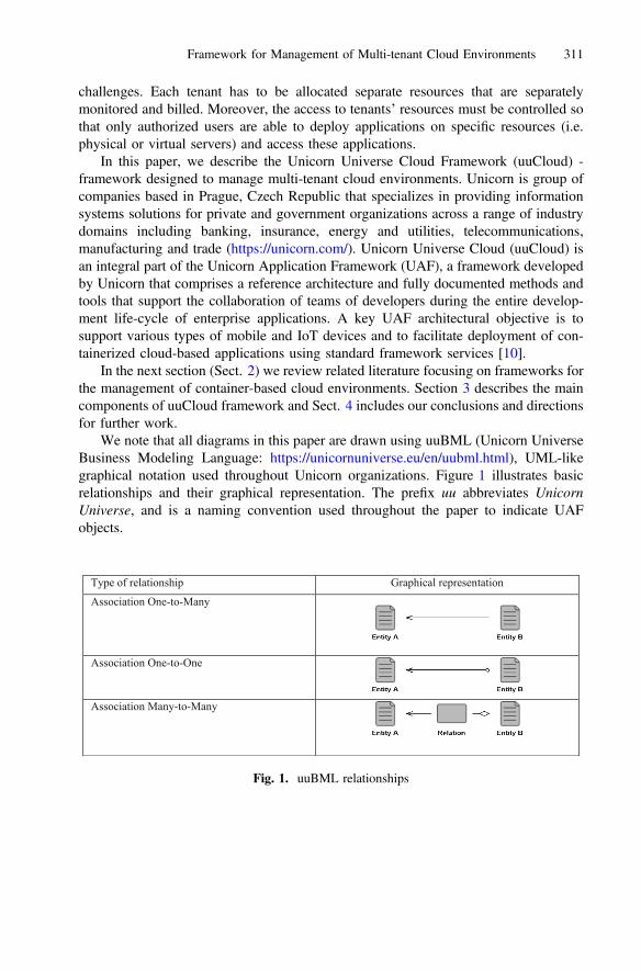
challenges. Each tenant has to be allocated separate resources that are separatelymonitored and billed. Moreover, the access to tenants’ resources must be controlled sothat only authorized users are able to deploy applications on specific resources (i.e.physical or virtual servers) and access these applications.
In this paper, we describe the Unicorn Universe Cloud Framework (uuCloud) -framework designed to manage multi-tenant cloud environments. Unicorn is group ofcompanies based in Prague, Czech Republic that specializes in providing informationsystems solutions for private and government organizations across a range of industrydomains including banking, insurance, energy and utilities, telecommunications,manufacturing and trade (https://unicorn.com/). Unicorn Universe Cloud (uuCloud) isan integral part of the Unicorn Application Framework (UAF), a framework developedby Unicorn that comprises a reference architecture and fully documented methods andtools that support the collaboration of teams of developers during the entire develop-ment life-cycle of enterprise applications. A key UAF architectural objective is tosupport various types of mobile and IoT devices and to facilitate deployment of con-tainerized cloud-based applications using standard framework services [10].
In the next section (Sect. 2) we review related literature focusing on frameworks forthe management of container-based cloud environments. Section 3 describes the maincomponents of uuCloud framework and Sect. 4 includes our conclusions and directionsfor further work.
We note that all diagrams in this paper are drawn using uuBML (Unicorn UniverseBusiness Modeling Language: https://unicornuniverse.eu/en/uubml.html), UML-likegraphical notation used throughout Unicorn organizations. Figure 1 illustrates basicrelationships and their graphical representation. The prefix uu abbreviates UnicornUniverse, and is a naming convention used throughout the paper to indicate UAFobjects.
Type of relationship Graphical representation
Association One-to-Many
Association One-to-One
Association Many-to-Many
Fig. 1. uuBML relationships
Framework for Management of Multi-tenant Cloud Environments 311
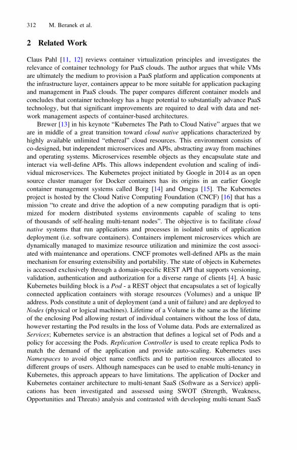
2 Related Work
Claus Pahl [11, 12] reviews container virtualization principles and investigates therelevance of container technology for PaaS clouds. The author argues that while VMsare ultimately the medium to provision a PaaS platform and application components atthe infrastructure layer, containers appear to be more suitable for application packagingand management in PaaS clouds. The paper compares different container models andconcludes that container technology has a huge potential to substantially advance PaaStechnology, but that significant improvements are required to deal with data and net-work management aspects of container-based architectures.
Brewer [13] in his keynote “Kubernetes The Path to Cloud Native” argues that weare in middle of a great transition toward cloud native applications characterized byhighly available unlimited “ethereal” cloud resources. This environment consists ofco-designed, but independent microservices and APIs, abstracting away from machinesand operating systems. Microservices resemble objects as they encapsulate state andinteract via well-define APIs. This allows independent evolution and scaling of indi-vidual microservices. The Kubernetes project initiated by Google in 2014 as an opensource cluster manager for Docker containers has its origins in an earlier Googlecontainer management systems called Borg [14] and Omega [15]. The Kubernetesproject is hosted by the Cloud Native Computing Foundation (CNCF) [16] that has amission “to create and drive the adoption of a new computing paradigm that is opti-mized for modern distributed systems environments capable of scaling to tensof thousands of self-healing multi-tenant nodes”. The objective is to facilitate cloudnative systems that run applications and processes in isolated units of applicationdeployment (i.e. software containers). Containers implement microservices which aredynamically managed to maximize resource utilization and minimize the cost associ-ated with maintenance and operations. CNCF promotes well-defined APIs as the mainmechanism for ensuring extensibility and portability. The state of objects in Kubernetesis accessed exclusively through a domain-specific REST API that supports versioning,validation, authentication and authorization for a diverse range of clients [4]. A basicKubernetes building block is a Pod - a REST object that encapsulates a set of logicallyconnected application containers with storage resources (Volumes) and a unique IPaddress. Pods constitute a unit of deployment (and a unit of failure) and are deployed toNodes (physical or logical machines). Lifetime of a Volume is the same as the lifetimeof the enclosing Pod allowing restart of individual containers without the loss of data,however restarting the Pod results in the loss of Volume data. Pods are externalized asServices; Kubernetes service is an abstraction that defines a logical set of Pods and apolicy for accessing the Pods. Replication Controller is used to create replica Pods tomatch the demand of the application and provide auto-scaling. Kubernetes usesNamespaces to avoid object name conflicts and to partition resources allocated todifferent groups of users. Although namespaces can be used to enable multi-tenancy inKubernetes, this approach appears to have limitations. The application of Docker andKubernetes container architecture to multi-tenant SaaS (Software as a Service) appli-cations has been investigated and assessed using SWOT (Strength, Weakness,Opportunities and Threats) analysis and contrasted with developing multi-tenant SaaS
312 M. Beranek et al.

applications using middleware services [17]. The authors conclude that more researchis needed to understand the true potential and risks associated with container orches-tration platforms such as Kubernetes. Other authors have considered multi-tenancyfrom the viewpoint of security challenges and proposed a model for identifying sus-picious tenant activities [18].
Other efforts in this area include OpensStack [19] - a cloud operating systemdesigned to control large pools of compute, storage, and networking resources.Administrators manage resources using a dashboard, and provision resources through aweb interface. In [20], the authors argue that many existing frameworks have a highdegree of centralization and do not tolerate system component failures; they present thedesign, implementation and evaluation of a scalable and autonomic virtual machine(VM) management framework called Snooze.
Li et al. [21] describe a REST service framework based on the concept ofResource-Oriented Network (RON). The authors discuss the advantages ofcontainer-based virtualization over VMs (Virtual Machines) that include lower CPUand memory consumption, faster reboot time, and significantly higher deploymentdensity (6–12 times), requiring fewer physical servers for the same workload andresulting in significant savings in capital expenditure. They identify a trend towardsRaaS (Resource-as-a-Service) that allows consumers to rent fine-grained resourcessuch as memory, CPU and storage on demand for short periods of time. The authorspoint out advances in Network Functions Virtualization (NFV) that make it possible tocontrol network elements, and advances in computer architecture that make it possibleto disaggregate CPU cores from the internal memory. The authors argue that a newservice abstraction layer is required to control and monitor fine-grained resources andto overcome the heterogeneity of the underlying Linux resource control models. Theyand note that RaaS cloud brings new challenges, in particular the ability to efficientlycontrol a very large number of fine-grain resources that are rented for short periods oftime. According to Ben-Yehuda [22], the trend toward increasingly finer resourcegranularity is set to continue resulting in increased flexibility and efficiency ofcloud-based solutions. Resources such as compute, memory, I/O, storage, etc. will becharged for in dynamically changing amounts, not in fixed bundles. The authors drawan analogy between cloud providers and phone companies that have progressed frombilling landlines per several minutes to billing cellphones by the minute, or even persecond. They conclude that the RaaS cloud requires new mechanisms for allocating,metering, charging for, reclaiming, and redistributing CPU, memory, and I/O resourcesamong multiple clients every few seconds.
In another publication [23] the authors explore the potential of vertical scalability,and propose a system for autonomic vertical elasticity of Docker containers (Elas-ticDocker). ElasticDocker performs live migration when the resources on the hostingmachine are exhausted. Experimental results show improved efficiency of livemigration technique, with a gain of 37.63% when compared to Kubernetes. As a resultof increase or decrease of workload, ElasticDocker scales up and down CPU andmemory assigned to containers, modifying resource limits directly in the Linux controlgroups (cgroups) associated with Docker containers. When the host resource limits arereached, the container is migrated to another host (i.e. the container image is transferredfrom a source to a target host). The authors argue that vertical scalability has many
Framework for Management of Multi-tenant Cloud Environments 313

benefits when compared to horizontal scalability, including fine-grained scaling andavoiding the need for additional resources such as load balancers or replicated instancesand delays caused by starting up new instances. Furthermore, horizontal scalability isonly applicable to applications that can be replicated and decomposed into independentcomponents. The experimental verification was performed using Kubernetes platformrunning CentOS Linux 7.2 on 4 nodes compared to running identical workload onElasticDocker, showing an improvement in the average total execution time of almost40%.
While Kubernetes appears to be gaining momentum as a platform for the man-agement of cloud resources with support for major public cloud platforms includingGoogle Cloud Platform, Microsoft Azure, and most recently Amazon AWS, there is anumber of other projects that aim to address the need for universal framework for thedevelopment and deployment of cloud applications. This rapidly evolving area is ofresearch interest to both academia and industry practitioners, but currently there is lackof agreement about a standard application framework designed specifically for clouddevelopment and deployment. This is particularly true in the context of multi-tenantcloud applications where the framework needs to support the management of resourcesallocated to a large number of individual tenants, potentially across multiple publiccloud platforms. Moreover, some proposals lack empirical verification usinglarge-scale real-life applications. Further complicating the situation is the rapid rate ofinnovation in this area characterized by the current trend toward increasingly finerresource granularity with corresponding impact on the complexity of cloud resourcemanagement frameworks.
3 Unicorn Universe Cloud (uuCloud)
uuCloud framework facilitates the provisioning of elastic cloud services using con-tainers and virtual servers, and consist of two basic components: the uuCloud Oper-ation Registry (uuOR) - a database that maintains active information about uuCloudobjects, and the uuCloud Control Centre (uuC3) - a tool that is used to automatedeployment and operation of container-based microservices. To ensure portability andto reduce overheads, uuCloud uses Docker [24] container-based virtualization. Dockercontainers can be deployed either to a public cloud infrastructure (e.g. AWS orMicrosoft Azure) or to a private (on-premises) infrastructure (e.g. Plus4U – UnicornUniverse cloud infrastructure). uuCloud supports the deployment of virtualized Uni-corn Universe Applications (uuApps). uuApp implements a cohesive set of functions,and in general is composed of sub-applications (uuSubApps); each uuSubApp is anindependent unit of functionality that implements a specific business use case (e.g.booking a visit to a doctor’s surgery). We made an architectural decision to implementeach uuSubApp as a containerized microservice using a Docker container.
Access to sub-applications is controlled using identities that are derived from userRoles (typically derived from the organizational structure), and are assigned to usersand system commands. The uuCloud security model is based on a combination ofApplication Profiles (collection of application functions that the application executes)and Application Workspaces (collection of application objects). Access to Application
314 M. Beranek et al.
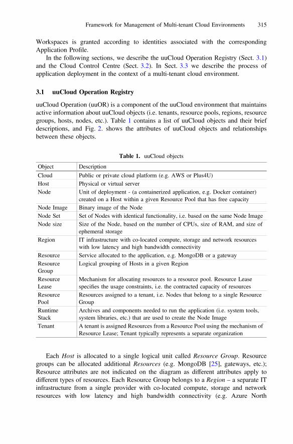
Workspaces is granted according to identities associated with the correspondingApplication Profile.
In the following sections, we describe the uuCloud Operation Registry (Sect. 3.1)and the Cloud Control Centre (Sect. 3.2). In Sect. 3.3 we describe the process ofapplication deployment in the context of a multi-tenant cloud environment.
3.1 uuCloud Operation Registry
uuCloud Operation (uuOR) is a component of the uuCloud environment that maintainsactive information about uuCloud objects (i.e. tenants, resource pools, regions, resourcegroups, hosts, nodes, etc.). Table 1 contains a list of uuCloud objects and their briefdescriptions, and Fig. 2. shows the attributes of uuCloud objects and relationshipsbetween these objects.
Each Host is allocated to a single logical unit called Resource Group. Resourcegroups can be allocated additional Resources (e.g. MongoDB [25], gateways, etc.);Resource attributes are not indicated on the diagram as different attributes apply todifferent types of resources. Each Resource Group belongs to a Region – a separate ITinfrastructure from a single provider with co-located compute, storage and networkresources with low latency and high bandwidth connectivity (e.g. Azure North
Table 1. uuCloud objects
Object Description
Cloud Public or private cloud platform (e.g. AWS or Plus4U)Host Physical or virtual serverNode Unit of deployment - (a containerized application, e.g. Docker container)
created on a Host within a given Resource Pool that has free capacityNode Image Binary image of the NodeNode Set Set of Nodes with identical functionality, i.e. based on the same Node ImageNode size Size of the Node, based on the number of CPUs, size of RAM, and size of
ephemeral storageRegion IT infrastructure with co-located compute, storage and network resources
with low latency and high bandwidth connectivityResource Service allocated to the application, e.g. MongoDB or a gatewayResourceGroup
Logical grouping of Hosts in a given Region
ResourceLease
Mechanism for allocating resources to a resource pool. Resource Leasespecifies the usage constraints, i.e. the contracted capacity of resources
ResourcePool
Resources assigned to a tenant, i.e. Nodes that belong to a single ResourceGroup
RuntimeStack
Archives and components needed to run the application (i.e. system tools,system libraries, etc.) that are used to create the Node Image
Tenant A tenant is assigned Resources from a Resource Pool using the mechanism ofResource Lease; Tenant typically represents a separate organization
Framework for Management of Multi-tenant Cloud Environments 315

(EU-N-AZ)). Regions are grouped into a (hybrid) Cloud that can be composed ofmultiple public (e.g. AWS, Microsoft Azure) and private clouds (e.g. Plus4U).
uuCloud supports multi-tenant operation; each Tenant typically represents a sep-arate organization (e.g. a doctor’s surgery). Tenants are assigned resources fromResource Pools using the mechanism of Resource Lease that specifies the usageconstraints, such as the contracted capacity, free capacity, etc. A Resource Pool definesthe maximum amount of resources (i.e. number of vCPUs, RAM size, size of storage,etc.) that are available for the operation of a specific Tenant. A Tenant can be allocatedseveral Resource Pools, for example separate Resource Pool for production anddevelopment, preventing application development from consuming productionresources. Each Tenant consumes its own resources and is monitored and billed sep-arately. Applications can be shared among multiple Tenants using the Share command(see Table 2), with the Tenant in whose Resource Pool the application is deployedbeing responsible for the consumed resources.
3.2 Cloud Control Center
The Operation Registry described in the previous section stores and manages uuCloudmetadata and is used by the Cloud Control Center (uuC3) to automate the managementand operation of container-based microservices deployed on public or private cloudinfrastructure. The Operation Registry database is managed using REST commands
Fig. 2. Structure of the uuCloud Operation Registry
316 M. Beranek et al.

that include commands for creating and deleting repository objects and commands forgenerating various repository reports. uuC3 defines an API that abstracts the com-plexity of the proprietary cloud infrastructures and supports node deployment and hostmanagement operations listed in Table 2.
3.3 Application Deployment Process
The first step in the application deployment process is to create a Node Image. Asillustrated in Fig. 3, Node Image is created from a uuSubApp and a Runtime Stack thatcontains all the related archives and components needed to run the application (i.e.system tools, system libraries, etc.). During deployment, the uuC3 applicationdeployment command (Deploy) reads the corresponding Deployment Descriptor(JSON file that contains parameter that define the application runtime environment).The resulting Node Image constitutes a unit of deployment. Node Image metadata arerecorded in the uuOR and the Node Image is published to the private Docker ImageRegistry.
The JSON code fragment in Fig. 4 shows the structure of the deployment descriptor,and the Table 3 below contains the description of the Deployment Descriptor attributes.
Figure 5 shows the relationship between objects used during the process ofdeployment of containerized applications. Node (i.e. Docker container) is a unit ofdeployment with characteristics that include virtual CPU (vCPU) count, RAM size and
Table 2. uuC3 REST API
Operation Description
Deploy Deploys a specified application (uuSubApp) to a specifiedResource Pool
Redeploy Redeploys a specified application (uuSubApp) to a specifiedResource Pool
Undeploy Undeploys a specified application (uuSubApp) from theResourcePool, deletes its Nodes, and releases all associatedresources
Reinit Reinitializes the specified Host to a consistent state as per uuORScale Increases or decreases the number of deployed NodesShare Shares the specified application (uuSubApp) with specified
tenantsUnshare Terminates sharing of the specified application (uuSubApp) with
the specified tenantgetAppDeploymentList Returns a list of applications (uuSubApps) and their Nodes
deployed to a specified Resource PoolgetAttributes Returns the attributes for a specified application (uuSubApps)
deploymentgetResourcePoolCapacity Returns information about Resource Pool CapacitygetStatus Returns the status of a specified hostgetNodeImageList Returns the list of node images
Framework for Management of Multi-tenant Cloud Environments 317
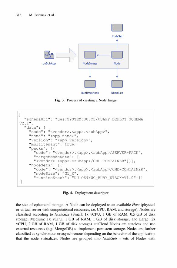
the size of ephemeral storage. A Node can be deployed to an available Host (physicalor virtual server with computational resources, i.e. CPU, RAM, and storage). Nodes areclassified according to NodeSize (Small: 1x vCPU, 1 GB of RAM, 0.5 GB of diskstorage, Medium: 1x vCPU, 1 GB of RAM, 1 GB of disk storage, and Large: 2xvCPU, 2 GB of RAM, 1 GB of disk storage). uuCloud Nodes are stateless and useexternal resources (e.g. MongoDB) to implement persistent storage. Nodes are furtherclassified as synchronous or asynchronous depending on the behavior of the applicationthat the node virtualizes. Nodes are grouped into NodeSets - sets of Nodes with
Fig. 3. Process of creating a Node Image
{
{
"schemaUri": "ues:SYSTEM:UU.OS/UUAPP-DEPLOY-SCHEMA-V2.1","data": {"code": "<vendor>.<app>.<subApp>","name": "<app name>","version": "<app version>","multitenant": true,"packs": [{"code": "<vendor>.<app>.<subApp>/SERVER-PACK","targetNodeSets": ["<vendor>.<app>.<subApp>/CMD-CONTAINER"]}],
"nodeSets": [{"code": "<vendor>.<app>.<subApp>/CMD-CONTAINER","nodeSize": "G1_M","runtimeStack": "UU.OS9/UC_RUBY_STACK-V1.0"}]}
Fig. 4. Deployment descriptor
318 M. Beranek et al.
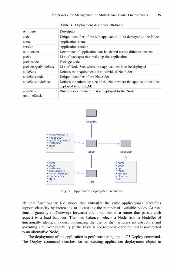
identical functionality (i.e. nodes that virtualize the same applications). NodeSetssupport elasticity by increasing or decreasing the number of available nodes. At run-time, a gateway (uuGateway) forwards client requests to a router that passes eachrequest to a load balancer. The load balancer selects a Node from a NodeSet offunctionally identical nodes, optimizing the use of the hardware infrastructure andproviding a failover capability (if the Node is not responsive the request is re-directedto an alternative Node).
The deployment of the application is performed using the uuC3 Deploy command.The Deploy command searches for an existing application deployment object in
Table 3. Deployment descriptor attributes
Attribute Description
code Unique identifier of the sub-application to be deployed to the Nodename Application nameversion Application versionmultitenant Determines if application can be shared across different tenantspacks List of packages that make up the applicationpacks:code Package codepacks:targetNodeSets List of Node Sets where the applications is to be deployednodeSets Defines the requirements for individual Node SetsnodeSets:code Unique identifier of the Node SetnodeSets.nodeSize Defines the minimum size of the Node where the application can be
deployed (e.g. G1_M)nodeSets.runtimeStack
Runtime environment that is deployed to the Node
Fig. 5. Application deployment scenario
Framework for Management of Multi-tenant Cloud Environments 319

uuOperation Registry, which can be identified by a composite key (ResourcePool URI,ASID, uuAppBox URI). If the deployment already exists, it will be updated, else a newapplication deployment is created for each instance of a particular application(uuSubApp).
The input parameters of uuC3 Deploy command in the code fragment illustrated inFig. 6 include: DEPLOY_POOL_URI (URI of the Resource Pool that the application isto be deployed into), appBoxUri (URI of the application distribution package), ASID(Application Server Identifier) – an application identifier generated by uuCloud touniquely identify each sub-application, uuEEs (list of identities that the applicationuses), TID (Tenant Identifier of the Tenant whose resources the application uses),uuSubAppDataStoreMap (mapping between the logical SubApplication Data Store andthe physical Data Store identifier values), privilegedUserMap (mapping between log-ical identity names and the actual user identities that are associated with access rights),uuSubAppInstanceSysOwner (identity of the system user who is authorized to deploythe application).
4 Conclusions
Wide-spread adoption of cloud computing and extensive use of mobile and IoT deviceshave impacted on the architecture of enterprise applications with corresponding impacton application development frameworks [26]. Microservices architecture has evolvedfrom SOA (Service Oriented Architecture) and is currently the most popular approachto implementing cloud-based applications. However, the management of large-scalecontainer-based microservices requires automation to ensure fast and predictableapplication deployment, auto-scaling and control of resource usage. Platforms and
UU::C3::AppDeployment.deploy('<DEPLOY_POOL_URI>',appBoxUri: '<APPBOX_URI>',asid: '<ASID>',uuEEs: ['<SYS_OWNER_UID>'],config: {tid: '<TID>',asid: '<ASID>',uuSubAppDataStoreMap: {primary: '<OSID>'
},privilegedUserMap: {uuSubAppInstanceSysOwner: '<SYS_OWNER_UID>'
}})
Fig. 6. uuC3 Deploy command
320 M. Beranek et al.

frameworks that support the development and deployment of container-based appli-cations have become an active area of research and development, and a number of opensource projects have been recently initiated. Kubernetes project, in particular, appearsto be gaining acceptance by major public cloud providers including Google, Microsoftand most recently Amazon AWS, as well as other important industry players. However,currently there is a lack of agreement about a standard application developmentframework designed specifically for cloud development and deployment. This situationis further complicated by the high rate of innovation in this area. It is quite likely thatthe present approach of implementing applications as containerized microservices willevolve to take advantage of much finer grained cloud resources with dramatic impacton the design, implementation and operation of cloud-based applications.
In this paper, we have described the uuCloud framework that is designed tofacilitate the management of large-scale container-based microservices with specificextensions to handle multi-tenancy. An important benefit of the uuCloud framework isits ability to manage complex multi-tenant environments deployed across multiple(hybrid) cloud platforms, hiding the heterogeneity of the underlying infrastructures (i.e.hardware, operating systems, virtualization technologies, etc.). uuCloud manages cloudmetadata, supports automatic application deployment and autonomic scaling ofapplications.
We are continuously monitoring the rapidly evolving landscape of cloud man-agement platforms and frameworks, and we may consider alignment of the uuCloudframework with Kubernetes in the future as both frameworks mature and the directionof cloud standardization becomes clearer.
References
1. Forester: The Public Cloud Services Market Will Grow Rapidly to $236 Billion in 2020(2018). https://www.forrester.com/. Accessed 10 Feb 2018
2. AWS: Amazon Web Services (AWS) - Cloud Computing Services (2018). https://aws.amazon.com/. Accessed 2 Feb 2018
3. Microsoft: Windows Azure Platform. http://www.microsoft.com/windowsazure/. Accessed10 Feb 2018
4. Burns, B., et al.: Borg, omega, and kubernetes. Queue 14(1), 10 (2016)5. Balalaie, A., Heydarnoori, A., Jamshidi, P.: Microservices architecture enables devops:
migration to a cloud-native architecture. IEEE Softw. 33(3), 42–52 (2016)6. CloudFoundry: Cloud Application Platform - Devops Platform—Cloud Foundry (2017).
https://www.cloudfoundry.org/. Accessed 28 Sept 20177. OpenShift: Container Application Platform by Red Hat, Built on Docker and Kubernetes
(2017). https://www.openshift.com/. Accessed 28 Sept 20178. OpenStack: OpenStack Open Source Cloud Computing Software (2018). https://www.
openstack.org/. Accessed 2 Feb 20189. Kubernetes (2017). https://kubernetes.io/. Accessed 25 Aug 201710. Beránek, M., Feuerlicht, G., Kovář, V.: Developing enterprise applications for cloud: the
unicorn application framework. In: International Conference on Grid, Cloud and ClusterComputing, GCC 2017, CSREA Press, Las Vegas, USA (2017)
Framework for Management of Multi-tenant Cloud Environments 321

11. Pahl, C., et al.: Cloud container technologies: a state-of-the-art review. IEEE Trans. CloudComput. 1 (2017). https://doi.org/10.1109/TCC.2017.2702586
12. Pahl, C.: Containerization and the PAAS cloud. IEEE Cloud Comput. 2(3), 24–31 (2015)13. Brewer, E.A.: Kubernetes and the path to cloud native. In: Proceedings of the Sixth ACM
Symposium on Cloud Computing. ACM (2015)14. Burns, B., et al.: Borg, omega, and kubernetes. Queue 14(1), 70–93 (2016)15. Schwarzkopf, M., et al.: Omega: flexible, scalable schedulers for large compute clusters. In:
Proceedings of the 8th ACM European Conference on Computer Systems. ACM (2013)16. Home - Cloud Native Computing Foundation (2017). https://www.cncf.io/. Accessed 27
Sept 201717. Truyen, E., et al.: Towards a container-based architecture for multi-tenant SaaS applications.
In: Proceedings of the 15th International Workshop on Adaptive and Reflective Middleware2016. ACM, Trento, Italy, pp. 1–6 (2016)
18. AlJahdali, H., et al.: Multi-tenancy in cloud computing. In: 2014 IEEE 8th InternationalSymposium on Service Oriented System Engineering (SOSE). IEEE (2014)
19. Kumar, R., et al.: Open source solution for cloud computing platform using OpenStack. Int.J. Comput. Sci. Mob. Comput. 3(5), 89–98 (2014)
20. Feller, E., Rilling, L., Morin, C.: Snooze: a scalable and autonomic virtual machinemanagement framework for private clouds. In: Proceedings of the 2012 12th IEEE/ACMInternational Symposium on Cluster, Cloud and Grid Computing (ccgrid 2012). IEEEComputer Society (2012)
21. Li, L., Tang, T., Chou, W.: A rest service framework for fine-grained resource managementin container-based cloud. In: 2015 IEEE 8th International Conference on Cloud Computing(CLOUD). IEEE (2015)
22. Agmon Ben-Yehuda, O., et al.: The rise of RaaS: the resource-as-a-service cloud. Commun.ACM 57(7), 76–84 (2014)
23. Al-Dhuraibi, Y., et al.: Autonomic vertical elasticity of docker containers with elasticdocker.In: 2017 IEEE 10th International Conference on Cloud Computing (CLOUD). IEEE (2017)
24. Docker: What is Docker, 14 May 2015. https://www.docker.com/what-docker. Accessed 21Aug 2017
25. MongoDB for GIANT Ideas (2017). https://www.mongodb.com/index. Accessed 21 Aug2017
26. Raj, P., Venkatesh, V., Amirtharajan, R.: Envisioning the cloud-induced transformations inthe software engineering discipline. In: Mahmood, Z., Saeed, S. (eds.) Software EngineeringFrameworks for the Cloud Computing Paradigm, pp. 25–53. Springer, London (2013).https://doi.org/10.1007/978-1-4471-5031-2_2
322 M. Beranek et al.
Fault Tolerant VM Consolidation forEnergy-Efficient Cloud Environments
Cihan Secinti(B) and Tolga Ovatman
Department of Computer Engineering, Istanbul Technical University,Istanbul, Turkey
{secintic,ovatman}@itu.edu.tr
Abstract. Cloud computing applications are expected to guarantee theservice performance which is determined by the Service Level Agreement(SLA) between cloud owner and client. While satisfying SLA, VirtualMachines (VMs) may be consolidated based on their utilization in orderto balance the load or optimize energy efficiency of physical resources.Since, these physical resources are prone to system failure, any optimiza-tion approach should consider the probability of a failure on a physicalresource and orchestrate the VMs over the physical plane accordingly.Otherwise, it is possible to experience unfavorable results such as numer-ous redundant application migrations and consolidations of VMs thatmay easily cause in SLA violations. In this paper, a novel approachis proposed to reduce energy consumption and number of applicationmigration without violating SLA while considering the fault toleranceof the cloud system in the face of physical resource failures. Simulationresults show that proposed model reduce energy consumption by approx-imately 37% and number of application migration by approximately 9%.Besides, in case of faults the increase of energy consumption is less than11% when the proposed approach is used.
Keywords: VM consolidation · Fault tolerance · Cloud computingGreen cloud · Live-migration · Application migration
1 Introduction
Cloud computing has many trending features such as on-demand services, virtu-alization and automatic scaling which leads remarkable increase in cloud usage.Data centers that host major cloud services contain enormous servers whichcause tremendously high energy consumption levels [1]. Along with the increasein the number of cloud users and powerful data centers, energy consumption ofcloud systems gained significant importance [2,3] over the last decade.
Growing importance of energy efficiency in cloud systems caused recent aca-demic studies to concentrate on energy efficiency on cloud systems as well. Inthis manner, virtual machine (VM) consolidation is a widely used method topromote more efficient energy consumption and utilization. On the other hand,c© Springer International Publishing AG, part of Springer Nature 2018M. Luo and L.-J. Zhang (Eds.): CLOUD 2018, LNCS 10967, pp. 323–333, 2018.https://doi.org/10.1007/978-3-319-94295-7_22
324 C. Secinti and T. Ovatman
in cloud computing, service performance is leveraged mostly with automaticscaling that may frequently led over-provisioned infrastructure and high energyconsumption.
Automatic scaling can be achieved in terms of vertical scaling and horizontalscaling. In this paper, horizontal scaling is focused where VM creation and VMconsolidation policies becomes important aspects of energy consumption trade-offs.
VM consolidation can be used as a means to reduce energy consumptionand optimize the VM utilization in horizontal scaling process. Consolidatingapplications in multiple VMs into a single VM may cause high utilization andreduced fault tolerance. Fault tolerance can be achieved either using a reactiveapproach or a proactive approach. Reactive fault tolerance policies aim to reducethe damage of failures after the failure whereas, proactive fault tolerance policiestry to predict the faults and reacts before the failure [4].
In modern cloud systems, three aspects; fault tolerance, energy efficiencyand performance requirements form a trade-off. High performance and fault tol-erant cloud environments require horizontal scaling, and energy efficient cloudsystems need VM consolidation for preventing unnecessary energy consumption.An approach is necessary to keep fault tolerance, energy efficiency and perfor-mance requirements in an optimized balance.
In this paper, a reactive fault tolerance approach is proposed for cloud envi-ronments which try to minimize the energy consumption by using VM consolida-tion. There are three different cases in the study; no-consolidation, consolidationby threshold and consolidation according to fault tolerant consolidation algo-rithm (FTC). No-consolidation case is presented as the control experiment forthe proposed approaches; when a new VM is created it will not be consolidatedeven if it runs no applications. In the second case, consolidation by threshold,VMs would be consolidated when their utilization is less then defined thresholdvalue. In the last case, FTC algorithm is used to accept or reject consolidationby threshold requests using the measure defined latter in the paper.
Major contributions of this paper are:
1. A novel measure to evaluate fault tolerance vulnerabilities.2. An algorithm (FTC) to orchestrate energy efficiency and fault tolerance
together.3. Simulating application placement, VM consolidation and fault tolerance
together to analyze trade-offs among them.4. Reduced number of application migration and energy consumption in hori-
zontal scaling.
The rest of this paper is organized as follows. The related work in this researchfield is presented in Sect. 2. Then, the simulation system features and structuraldetails are described in Sect. 3. In Sect. 4, experiment details and results arepresented, finally, followed by conclusion and planned future work in the lastsection.

Fault Tolerant VM Consolidation for Energy-Efficient Cloud 325
2 Related Work
VM consolidation has become a significant technique for data center energyand resource management. For consolidation of VM several methods are car-ried on already such as Ant Colony Optimization, K-Nearest Neighbor, GreedyHeuristics [5–7]. On the other hand, VM consolidation requires live migration ofthe applications which are hosted by the corresponding VM [8]. Besides in [9],authors analyzed CO2 emissions of the data centers by considering their energyconsumption in network level. In [3], the authors are proposed a model whichmigrates highly utilized virtual machines to the low utilized hosts while keepingthe energy efficiency of the data center by realizing firefly algorithm. However,these techniques do not consider the fault toleration of the VMs.
In the real world, cloud systems could encounter system failures by theirdynamic nature [10] which must be prevented to achieve guaranteed Quality ofService (QoS). Hence, various fault tolerant cloud environment approaches areinvestigated. In [11], fault occurrences are more similar to Weibull Distribution(WD).
The authors proposed an active replication model to provide fault tolerancein [12]. Then, in [13], the replication approach is further enhanced by usingbyzantine fault tolerance gain to optimize the overall cost. However, all of thesestudies require user experience and knowledge for configuration and applicationpreparation phase. Since most of the approaches utilize VM level live-migrationamong data centers to create fault tolerant cloud environment, the techniquesrepresented in [14] distinguishes these approaches by using application level live-migration.
In [15], the authors emphases the gap of fault tolerant, energy efficient cloudenvironment approaches by using VM consolidation.
3 Simulation System Structure of the Proposed Approach
Simulation software1 used in this study is developed in Java 8 and tested on PCwhich has Intel Core i7 7700HQ @ 2.80 GHz, 16 GB DDR4-2400, 4 GB NVidiaGTX1050, on a Windows 10 64-bit environment. Typically, a simulation runtakes 15 s. The application creation time and resource usage data are generatedrandomly by using uniform distribution. The simulation framework works foronly one physical machine and all the VMs are created and consolidated on thesame physical machine.
The main structure of the simulation is shown in Fig. 1. The simulation con-sists of two main phases; application assignment of VM and VM consolidationon physical machine. The application placement [16] is a divergent and huge areafor covering in this paper hence Round Robin algorithm is used to ease imple-mentation of this part. So, it is same for all three test cases (no-consolidation,consolidation by threshold, consolidation by FTC). The second phase of thesimulation is the main focus of enhancement.1 https://github.com/secintic/CloudSimulation.git.

326 C. Secinti and T. Ovatman
Fig. 1. Simulation flow chart
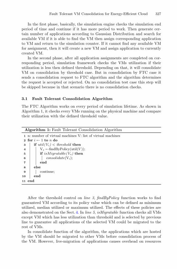
Fault Tolerant VM Consolidation for Energy-Efficient Cloud 327
In the first phase, basically, the simulation engine checks the simulation endperiod of time and continue if it has more period to work. Then generate cer-tain number of applications according to Gaussian Distribution and search foravailable VM if it is able to find the VM then assign corresponding applicationto VM and return to the simulation counter. If it cannot find any available VMfor assignment, then it will create a new VM and assign application to currentlycreated VM.
In the second phase, after all application assignments are completed on cor-responding period, simulation framework checks the VMs utilization if theirutilization is less then defined threshold. Depending on that, it will consolidateVM on consolidation by threshold case. But in consolidation by FTC case itsends a consolidation request to FTC algorithm and the algorithm determinesthe request is accepted or rejected. On no consolidation test case this step willbe skipped because in that scenario there is no consolidation checks.
3.1 Fault Tolerant Consolidation Algorithm
The FTC Algorithm works on every period of simulation lifetime. As shown inAlgorithm 1, it checks every VMs running on the physical machine and comparetheir utilization with the defined threshold value.
Algorithm 1: Fault Tolerant Consolidation Algorithm1 n: number of virtual machines V: list of virtual machines2 for i ← 1 to n do3 if util(Vi) < threshold then4 Vs ←findByPolicy(util(V ));5 if isMigratable(Vs) then6 consolidate(Vi);7 end
8 else9 continue;
10 end
11 end
After the threshold control on line 3, findByPolicy function works to findguaranteed VM according to its policy value which can be defined as minimumutilized, median utilized or maximum utilized. The effects of these policies arealso demonstrated on the Sect. 4. In line 5, isMigratable function checks all VMsexcept VM which has less utilization than threshold and is selected by previousline to guarantee all applications of the selected VM could be migrated to therest of VMs.
In consolidate function of the algorithm, the applications which are hostedby the VM should be migrated to other VMs before consolidation process ofthe VM. However, live-migration of applications causes overhead on resources

328 C. Secinti and T. Ovatman
consumption of the VMs which may easily result in higher energy consumptionby 10% [17]. Therefore, the key factor of the consolidation is to reduce numberof application migration to reduce energy consumption and it is not significantto migration application to which VM.
In general, the main purpose of the algorithm is to prevent new VM creationwhen a failure occurrence on any of the VMs. Therefore, it determines consol-idation request approval by checking the other VMs are capable of to manageall its applications. If they are capable then the algorithm will accept the con-solidation request and VM will be consolidated. Otherwise, the request will berejected and consolidation would not be happened.
Energy consumption of VMi is calculated in Eq. 1.
Ei = k +m∑
j =1
cpu(aj) + memory(aj) (1)
where variable k represents idle energy consumption, a denotes for applicationand m is the total number of applications hosted by VMi. cpu and memoryfunctions return the memory and CPU consumption of aj . The equation sumsthe idle energy consumption and all utilized resources (CPU and Memory in caseof suggested model) which is used by applications.
In Eq. 2, total energy consumption is calculated by using VM energy con-sumption and application migration’ energy overhead.
TE =n∑
i=1
(1 +s(p)10
) × Ei (2)
where variable s(p) represents the number of the application migration amongthe VMs on period p.
4 Simulation Results
In the simulation, energy consumption and number of the application migra-tions are compared for three different cases (no-consolidation, consolidation bythreshold and FTC) which are mentioned in Sect. 1.
Number of generated applications are shown in Fig. 2. To test model on afluctuating application generated environment several Gaussian Distributionsare overlapped independently from fault occurrence distribution.
In the first experiment, energy consumption on various threshold values arechecked for all cases. The threshold values are defined as utilization percentageof the VM and shown in Table 1. In the other experiments, number of applicationmigrations and energy consumption changes on simulation time are analyzed byusing a constant 50% threshold value.
Defined simulation variables are shown in Table 1. For resources types CPUand Memory are used and application resources consumption are selected fromuniform distribution on the interval of 0.1 and 0.3. The variables are defined

Fault Tolerant VM Consolidation for Energy-Efficient Cloud 329
Fig. 2. Application generation distribution
Table 1. Simulation variables
Variables Values
Resources {CPU, Memory}VM Capacities {CPU: 20, Memory: 20}Application resource consumption {CPU: 0.1 – 0.3, Memory: 0.1 – 0.3}Fault Occurrence times WD random points period: {49, 72,
88, 137, 157, 337, 364, 475, 733, 891}Simulation duration 1000 periods
Threshold (%) {30, 40, 50, 60, 70}
according to Google Cluster Data [18,19]. The VM capacities defined as 20core CPU and normalized 20 units of memory. Faults occurrences are gatheredfrom Weibull Distribution and it happens 10 times in a simulation lifetime. Thesimulation runs for 1000 period to collect results.
In Fig. 3, total energy consumption of the simulation lifetime has calculatedby using Eq. 2 for different threshold values. In No-consolidation case, modeldo not consolidate any VM and if it is necessary it creates new one so energyconsumption values are higher than other two case. In normal conditions, thethreshold value changes would not affect no-consolidation energy consumptionbut in this simulation model, faulty VM is selected randomly so it can be increasewhen occurred on VMs with high utilization or vice-versa. In Consolidationcase, keeping the threshold value low gives the advantage of reduced energyconsumption. Hence, consolidation of VMs with high utilization causes costly

330 C. Secinti and T. Ovatman
Fig. 3. Energy consumption comparison for different threshold values
application migrations because of having more number of applications also faultoccurrences affect Consolidation case worse than the other cases. The FTC modelis not affected from threshold value changes by the advantage of its rejectioncapability. But its slightly more robust on higher threshold values. Instead ofconsolidating low threshold VMs by considering fault possibility, consolidationof VMs with high threshold results the better energy efficiency. In results, theFTC approach has reduced energy consumption by 30% to 50%.
In Fig. 4, number of application migration and energy consumption of wholesystem are compared for all three test cases. the FTC algorithm has the min-imum number of application migration and also 50% less energy consumptionaccording to consolidation by threshold case. When an error occurred in allcases, applications are migrated from faulty VM to other VMs which causes toincrease of energy consumption on fault occurrence times of the simulation. TheFTC model degrades impacts of fault occurrence and prevents the unnecessaryapplication migrations for fault tolerance so it keeps energy consumption morestabilized.
In Fig. 5, three different guaranteed VM finder policies are compared; max-imum, minimum and median utilized as mentioned in Sect. 3. The results showthat if it is selected as minimum it will converge to the consolidation case, other-wise it is selected as two times maximum it will converge to the no-consolidationcase. The best results are found when the maximum utilized VM is selected andother VMs are checked by hosting the maximum utilized VM applications.

Fault Tolerant VM Consolidation for Energy-Efficient Cloud 331
Fig. 4. Threshold value is selected as 50%
Fig. 5. Max, Min, Median FTC Algorithm policies on 50% threshold value
5 Conclusion and Future Works
In this paper, a novel approach is proposed to satisfy fault tolerance and energyefficiency together. Hence, two different experiment are created to prove FTCmodel and its advantages. Energy consumption and number of application migra-

332 C. Secinti and T. Ovatman
tion results are compared under various threshold values. The experiments showthat with the FTC approach the energy consumption ca be reduced by 30% to50% and number of application migrations can be reduced by %10 in a faultycloud environment. The proposed approach also reduces the impact of faults onVMs.
In the future, the proposed approach is planned to be validated using differentreal-world data sets. An additional contribution to proposed approach can be toadapt machine learning techniques in order to perform time series analysis andsmart prediction of future fluctuations on VM resource demands.
References
1. Ghribi, C., Hadji, M., Zeghlache, D.: Energy efficient VM scheduling for clouddata centers: exact allocation and migration algorithms. In: 2013 13th IEEE/ACMInternational Symposium on Cluster, Cloud, and Grid Computing, pp. 671–678,May 2013. https://doi.org/10.1109/CCGrid.2013.89
2. Rodero, I., et al.: Energy-efficient thermal-aware autonomic management of virtu-alized HPC cloud infrastructure. J. Grid Comput. 10(3), 447–473 (2012). https://doi.org/10.1007/s10723-012-9219-2. ISSN 1572–9184
3. Kansal, N.J., Chana, I.: Energy-aware virtual machine migration for cloud com-puting - a firey optimization approach. J. Grid Comput. 14(2), 327–345 (2016).https://doi.org/10.1007/s10723-016-9364-0. ISSN 1572–9184
4. Bala, A., Chana, I.: Fault tolerance-challenges, techniques and implementation incloud computing. 9, January 2012
5. Farahnakian, F., et al.: Using Ant colony system to consolidate VMs for greencloud computing. IEEE Trans. Serv. Comput. 8(2), 187–198 (2015). https://doi.org/10.1109/TSC.2014.2382555. ISSN 1939–1374
6. Farahnakian, F., et al.: Utilization prediction aware VM consolidation approachfor green cloud computing. In: 2015 IEEE 8th International Conference on CloudComputing, pp. 381–388, June 2015. https://doi.org/10.1109/CLOUD.2015.58
7. Ferdaus, M.H., Murshed, M., Calheiros, R.N., Buyya, R.: Virtual machine con-solidation in cloud data centers using ACO metaheuristic. In: Silva, F., Dutra, I.,Santos Costa, V. (eds.) Euro-Par 2014. LNCS, vol. 8632, pp. 306–317. Springer,Cham (2014). https://doi.org/10.1007/978-3-319-09873-9 26
8. Ferdaus, M.H., et al.: Multi-objective, Decentralized Dynamic Virtual MachineConsolidation using ACO Metaheuristic in Computing Clouds. In: CoRRabs/1706.06646 (2017). arXiv: 1706.06646
9. Cavdar, D., Alagoz, F.: A survey of research on greening data centers. In: 2012IEEE Global Communications Conference (GLOBECOM), pp. 3237–3242, Decem-ber 2012. https://doi.org/10.1109/GLOCOM.2012.6503613
10. Amin, Z., Singh, H., Sethi, N.: Review on Fault tolerance techniques in cloudcomputing. Int. J. Comput. Appl. 116(18), 11–17 (2015)
11. Liu, J., et al.: A Weibull distribution accrual failure detector for cloud computing.PLOS ONE 12(3), 1–16 (2017). https://doi.org/10.1371/journal.pone.0173666
12. Santos, G.T., Lung, L.C., Montez, C.: FTWeb: a fault tolerant infrastructure forweb services. In: Ninth IEEE International EDOC Enterprise Computing Confer-ence (EDOC 2005), pp. 95–105, September 2005. https://doi.org/10.1109/EDOC.2005.15

Fault Tolerant VM Consolidation for Energy-Efficient Cloud 333
13. Wood, T., et al.: ZZ and the art of practical BFT execution. In: Proceedings ofthe Sixth Conference on Computer Systems, EuroSys 2011, pp. 123–138. ACM,Salzburg (2011). https://doi.org/10.1145/1966445.1966457
14. Cully, B., et al.: Remus: high availability via asynchronous virtual machine repli-cation. In: Proceedings of the 5th USENIX Symposium on Networked SystemsDesign and Implementation, NSDI 2008, pp. 161–174. USENIX Association, SanFrancisco (2008). http://dl.acm.org/citation.cfm?id=1387589.1387601
15. More, N.S., Ingle, R.B.: Challenges in green computing for energy saving tech-niques. In: 2017 International Conference on Emerging Trends Innovation in ICT(ICEI), pp. 73–76, February 2017. https://doi.org/10.1109/ETIICT.2017.7977013
16. Secinti, C., Ovatman, T.: On optimizing resource allocation and application place-ment costs in cloud systems. In: Proceedings of the 4th International Confer-ence on Cloud Computing and Services Science, CLOSER 2014, pp. 535–542.SCITEPRESS - Science and Technology Publications, LDA, Barcelona, (2014).https://doi.org/10.5220/0004849605350542. ISBN: 978-989-758-019-2
17. Voorsluys, W., Broberg, J., Venugopal, S., Buyya, R.: Cost of virtual machine livemigration in clouds: a performance evaluation. In: Jaatun, M.G., Zhao, G., Rong,C. (eds.) CloudCom 2009. LNCS, vol. 5931, pp. 254–265. Springer, Heidelberg(2009). https://doi.org/10.1007/978-3-642-10665-1 23
18. Reiss, C., Wilkes, J., Hellerstein, J.L.: Google cluster-usage traces: format +schema. Technical report, Google Inc., Mountain View, November 2011. Version2.1. https://github.com/google/cluster-data. Accessed 17 Nov 2014
19. Wilkes, J.: More Google cluster data. Google research blog. http://googleresearch.blogspot.com/2011/11/more-google-cluster-data.html, November 2011

Over-Sampling Algorithm Based on VAEin Imbalanced Classification
Chunkai Zhang1(&), Ying Zhou1, Yingyang Chen1, Yepeng Deng1,Xuan Wang1, Lifeng Dong2, and Haoyu Wei3
1 Harbin Institute of Technology Shenzhen Graduate School, Shenzhen, [email protected]
2 Hamline University, 1536 Hewitt Avenue, St. Paul, USA3 Sichuan University, Chengdu, Sichuan, China
Abstract. The imbalanced classification problem is a problem that violates theassumption of uniform distribution of samples, classes differ in sample size,sample distribution and misclassification cost. The traditional classifiers tend toignore the important minority samples because of their rarity. Oversampling, thealgorithm uses various methods to increase the minority samples in the trainingset to increase the recognition rate of them. However, these over-samplingmethods are too coarse to improve the classification effect of the minoritysamples, because they can’t make full use of the information in the originalsamples, but increase the training time because of adding extra samples. In thispaper, we propose to use the distribution information of the minority samples,use the variational auto-encoder to fit the probability distribution function ofthem without any prior assumption, and reasonably expand the minority classsample set. The experimental results prove the effectiveness of the proposedalgorithm.
Keywords: Imbalanced classification � Variational auto-encoderOversampling
1 Introduction
The classification problem is a very important part of machine learning, and it is alsothe first step for artificial intelligence to understand human life. At present, mostclassifiers assume that the samples of different classes are evenly distributed, and theclassification costs are the same. However, in reality, the data people are more con-cerned about is often scarce, such as the detection of credit card fraud and medicaldisease diagnosis. In the medical disease diagnosis, most of the results are normal whileonly a small proportion of the results are diagnosed as diseases, which indicates thedifferent distribution in different classes samples. Second, if healthy people are mis-diagnosed as diseases, they can be removed by other inspection methods, errors do notcause very serious accidents, but if the disease people are diagnosed as healthy, it maycause the patients to miss the best treatment time and cause serious consequences. Thisis the second feature of the imbalanced classification problems: different classes ofmisclassification costs are inconsistent. At the same time, if samples are classified as
© Springer International Publishing AG, part of Springer Nature 2018M. Luo and L.-J. Zhang (Eds.): CLOUD 2018, LNCS 10967, pp. 334–344, 2018.https://doi.org/10.1007/978-3-319-94295-7_23

diseases as much as possible because they are afraid to miss the disease samples, it willcause a huge waste of medical resources and intensify conflicts between doctors andpatients. Therefore, it is not feasible to determine all samples as disease, and the bestway is to try to separate these two results as correct as possible. Due to the scarcity ofthe minority samples and the definition of global accuracy, the classifier pays lessattention to the minority class, so the recognition performance is unsatisfying. Imbal-anced classification problems arise in many fields, such as bioinformatics [1, 2], remotesensing image recognition [3], and privacy protection in cybersecurity [4–6]. Theimbalanced problems cover widely and have a very important practical significance.
The traditional solutions to the imbalanced problems are divided into two parts: thealgorithm-level methods and the data-level methods. The algorithm-level methodsmainly focus on the different misclassification costs, such as improved neural network[7]: it uses the approximation of F1 value of the minority class as the cost function; thebagging algorithm [8] continues to enhance the misclassified the minority samples, andimprove the recognition rate of the minority samples; structured SVM [9] uses the F1value of the minority samples as the optimization function, and has a better perfor-mance in the classification of the minority samples.
The data-level methods focus on the imbalance of sample size, which mainly adjustthe data sample size through resampling to reduce the impact on classification per-formance. The data-level methods can be divided into over-sampling, under-samplingand hybrid sampling. Over-sampling adds the minority samples in the training process,Over-sampling can effectively improve the classification performance of the minorityclass but it has no idea of the rationality. Under-sampling [10] removes the majoritysamples before training, which can quickly reach equilibrium, but may take a risk oflosing valuable samples.
The oversampling method can be divided into random sampling and informedsampling. Random sampling means repeating the known samples, which includessimple repetition [11], linear interpolation [12], nonlinear interpolation [13], etc.;SMOTE [12], as a classic over-sampling algorithm, interpolates linearly in the minoritysamples, will increase the amount of information and rationality of synthesized samplesin random oversampling, which improves the classification effect. Border-line-smote[14], to reduce the risk of overfitting, it selects the minority samples needing to beinterpolated called boundary samples. The above oversampling methods only considerthe influence of the sample size and the local sample distribution on the classificationperformance, ignoring the overall distribution of the sample, which is more informativefor classification performance.
Informed sampling [15] uses the distribution information in the sample to fit itsprobability distribution function (PDF) and sample it according to the PDF. Chen [16]proposed a normal distribution based oversampling approach, and this approachassumes the minority class distribution as the Gaussian normal distribution, theparameters are calculated from the minority samples with EM algorithm, the experi-mental results are better than SMOTE and random oversampling. Different scholarshave proposed oversampling algorithms based on various distributions, such as theGaussian distribution [16, 17], Weibull distribution [18], etc. Due to the distributioninformation, these algorithms have made greater progress than random oversamplingmethod. However, the problems are also obvious: there is a prior assumption about the
Over-Sampling Algorithm Based on VAE in Imbalanced Classification 335

real distribution and all the features are dependent from each other. If the real distri-bution meets this hypothesis, it will get better results, otherwise, the improvement islimited, so it is inconsistent in their effect on different datasets.
Data level methods are of great matter in imbalanced classification, as it can beregarded as a step in data preprocessing, it will have a positive effect on the finalclassification results. Since the factors that affect the datasets classification include notonly the sample size, but also the sample distribution, while the current over-samplingmethods do not make full use of distribution information and cannot guarantee therationality of the generated samples.
In this paper, we propose a oversampling method based on the variationalauto-encoder [19] (VAE) model to generate the minority samples. The proposedmethod is motivated that the distribution information plays an important role inoversampling methods, and aims at the rationality of the generated samples, we useVAE to increase minority instances, to our knowledge, first, the output dimension ofthe neural network is not limited so it can generate data of any dimension; second, thestrong fitting ability of the neural network can simulate any distribution functionwithout any prior knowledge in advance. We use this model to model the distributionof minority samples and oversample according to the model, the proposed methodshows the superiority that it doesn’t need any prior distribution assumption nor thedependent features assumption, the experimental results prove the effectiveness of thealgorithm.
We organize the paper as follows. Section 2 describes related work of this paper.Section 3 presents the proposed algorithm and analyze it. Section 4 shows theexperimental results. Section 5 concludes the paper.
2 Related Work
In 2013, KM [19] proposed VAE: add variational inference to auto-encoder and useparameterization trick to make the variational inference combined with stochasticgradient descent. The overall structure of vae network is shown in Fig. 1, while itassumes the hidden variables to be a Gaussian standard distribution, it is easy to sampleand the final probability distribution function is uncertain, coincides with the charac-teristics of distribution-based oversampling.
In VAE, we assume the variables are determined by the hidden compression code z,the encoder can map z to X, which makes z obey a particular distribution (such asGaussian distribution, etc.). Knowing the possibility distribution function and itsmapping function, we can sample z and encode z, to get new x to generate infinitesample theoretically. The structure of vae as shown below:
Assume z is a latent variable, and its distribution function is p(z), use Bayesianconditional probability formula to calculate P(X):
p Xð Þ ¼ Zp Xjzð Þp zð Þ dz ð1Þ
However, in z’s prior distribution, most of z cannot generate reliable samples, that is p(X|z) tends to 0, so p(X|z)p(z) tends to 0. To simplify the calculation, only p(X│z) need
336 C. Zhang et al.

to be calculated. Considering the z with larger P(X|z), which is represented by P(z|X)form the encoder, but only considering this part of z cannot generate samples that are notin original data, so we need to assume the distribution of P(z│X) and complete the errorthrough the decoder.
Q(z) is the assumption of the real distribution, we use KL divergence to calculatethe difference between the real distribution and the assumption:
D(pjjq) ¼ Zp xð Þ log p xð Þ
q xð Þ dx ð2Þ
Formula (2) shows that if two distribution is close, KL divergence will tend to 0.And the loss function of VAE model is
argmin D(Q(z)jjP(zjX)) ð3Þ
Apply the formula (2) to the formula (3)
D½QðzÞjjP zjXð Þ� ¼ Ez�Q½log Q zð Þ � log P zjXð Þ� ð4Þ
Apply Bayes rule to PðzjXÞ, we can get both P Xð Þ and PðXjzÞ
DðQ zð ÞjjPðzjXÞÞ ¼ Ez�Q log Q zð Þ � log P zð Þ½ � þ log PðXÞ ð5Þ
Apply the D½QðzÞjjP zjXð Þ� into it, note that X is fixed, and Q can be any distri-bution, not just a distribution which does a good job at mapping X to the z’s to produceX. since we’re interested in inferring P(X), it makes sense to construct a Q which doesdepend on X, and in particular, one which makes DðQ zð ÞjjPðzjXÞÞ small: BecauseP Xð Þ is fixed, the minimum DðQ zð ÞjjP zjXð ÞÞ will transform to maximize the value ofthe right side of the equation, and log PðXjzÞ is the probability of X decoded by z. It iscalculated as the cross-entropy or mean-squared error of the original sample. The latter
Fig. 1. Structure of variational auto-encoder.
Over-Sampling Algorithm Based on VAE in Imbalanced Classification 337

can be regarded as the difference between the assumption and the distribution of z inthe encoder.
log P Xð Þ � D½QðzÞjjPðzjXÞ� ¼ Ez�Q log P Xjzð Þ½ � � D½Q½z�jjPðzÞ� ð6Þ
3 The Proposed Method
In this paper, an oversampling method based on VAE is proposed, motivated by theidea that the distribution information is important in oversampling method. Withoutany prior assumption of the real PDF of the minority samples nor the independentassumption in the features, the proposed method can automatically model the PDF withthe oral data. However, there is also a trick in the proposed, there might have discretefeatures in the data, while the features generated by the stochastic gradient descent mustbe continuously differentiable, so this part of the features must be selected before vaetraining using formula (9), and after generating the continuous features, use 1-NN toclassify the generated continuous and combine the continuous features with the discretefeatures of the nearest original sample into a new composite sample.
We don’t have enough information about whether a feature is discrete or not, so weassume that it is a discrete feature if there are no more than 2 distinct values in all thefeature values. In fact, it is useless in classification if there is only one distinct valueamong the whole dataset.
Given training dataset X ¼ x1; y1ð Þ; x2; y2ð Þ; � � � ; xN; yNð Þf g, xi 2 Rd is thesample of d dimension, yi 2 0; 1f g is the labels represent negative and positive. Weuse P and N to represents a positive class sample subset and a negative class samplesubset, where P contains Nþ positive samples, N contains N� negative samples, andNþ þN� ¼ N.
During the training of the VAE model, nelementsj represents the number of distinctfeature values in jth dimension in the positive subset, the formula is shown as (7):
nelementsj ¼XNþ
idistinct xij
� �; 1� j� d ð7Þ
xi ¼ xi1; xi2; � � � ; xikf g [ f xi kþ 1ð Þ; � � � ; xidg ð8Þ
s:t:nelementsj [ 2; 1� j� knelementsj � 2; kþ 1� j� d
�ð9Þ
If nelementsj is no more than 2, the feature j is discrete, otherwise, the feature iscontinuous. Divide the features in the positive subset into continuous and discretefeatures in order and the continuous features are used as the final training set.
Xtrainvae ¼x11 � � � x1k... . .
. ...
xNþ 1 � � � xNþ k
264
375 ð10Þ
338 C. Zhang et al.
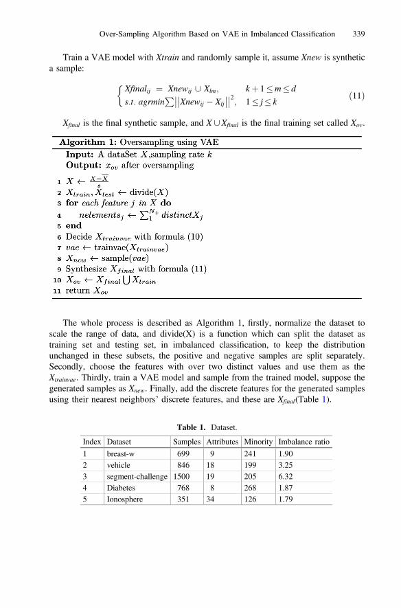
Train a VAE model with Xtrain and randomly sample it, assume Xnew is synthetica sample:
Xfinalij ¼ Xnewij [ Xlm; kþ 1�m� d
s:t: agrminP
Xnewij � Xlj
�� ���� ��2; 1� j� k
�ð11Þ
Xfinal is the final synthetic sample, and X [Xfinal is the final training set called Xov.
The whole process is described as Algorithm 1, firstly, normalize the dataset toscale the range of data, and divide(X) is a function which can split the dataset astraining set and testing set, in imbalanced classification, to keep the distributionunchanged in these subsets, the positive and negative samples are split separately.Secondly, choose the features with over two distinct values and use them as theXtrainvae. Thirdly, train a VAE model and sample from the trained model, suppose thegenerated samples as Xnew. Finally, add the discrete features for the generated samplesusing their nearest neighbors’ discrete features, and these are Xfinal(Table 1).
Table 1. Dataset.
Index Dataset Samples Attributes Minority Imbalance ratio
1 breast-w 699 9 241 1.902 vehicle 846 18 199 3.253 segment-challenge 1500 19 205 6.324 Diabetes 768 8 268 1.875 Ionosphere 351 34 126 1.79
Over-Sampling Algorithm Based on VAE in Imbalanced Classification 339

4 Experiment
4.1 Dataset and Evaluation
In this paper, all datasets are from UCI [20] Machine Learning Repository, and some ofthem are multi-label datasets, so we select one class as the minority class and theremaining samples as majority class. The missing values are supplemented by the mostfrequent value. After that we use normalization, the formula is shown in (12):
xinew ¼ xi � �xs
ð12Þ
�x ¼ 1n
Xn
i¼1xi; s ¼
ffiffiffiffiffiffiffiffiffiffiffiffiffiffiffiffiffiffiffiffiffiffiffiffiffiffiffiffiffiffiffiffiffiffiffiffiffiffiffiffiffiffiffiffiffi1
n� 1
Xn
iðxi � �xÞ
� �2s
ð13Þ
In traditional classification method, global accuracy is used as the evaluation, but inthe imbalanced problem, this evaluation will mask the classification performance of theminority class. In extreme conditions, assume the dataset only contain 1% minorityclass, if the classifier decides all samples as majority class, the accuracy still can reach99%, and however, the recognition rate of the minority samples is 0. In binaryimbalanced classification, the confusion matrix in Table 2. Confusion metrics. is oftenused to evaluate the performance of the classifier.
Among them, FN is the number of the positive samples misclassified as negative,and FP is the number of the negative samples misclassified as positive. There are somenew evaluation metrics based on confusion matrix to calculate the accuracy and recallof imbalance data such as F-value, G-mean [21].
precision ¼ TPTPþFP
ð14Þ
recall ¼ TPTPþFN
ð15Þ
F � value ¼ ð1þ b2Þ � recall � precision
b2 � recall þ precisionð16Þ
Where b 2 0; þ1½ �:
Table 2. Confusion metrics.
Positive prediction Negative prediction
Positive class True positive(TP) False negative(FN)Negative class False positive(FP) True negative(TN)
340 C. Zhang et al.

Gmean ¼ffiffiffiffiffiffiffiffiffiffiffiffiffiffiffiffiffiffiffiffiffiffiffiffiffiffiffiffiffiffiffiffiffiffiffiffiffiffiffiffiffiffiffiffiffiffi
TPTP + FN
� TNTN + FP
rð17Þ
In this experiment, we choose b ¼ 1 for F-value, it is the average between recalland precision. Gmean is the geometric mean of the classification accuracy of theminority class and majority class. Only when the precision of minority class andprecision of majority are high at the same time, gmean will be maximum.
4.2 Experiment Results
In this paper, we compare different oversampling algorithms such as NDO-sampling[17] and random interpolation algorithm SMOTE [12] (SMO). The classifier is naïveBayes to reduce the impact of classifier’s parameters on classification performance. Toreduce the randomness in the final results, each algorithm calculates the average of 10times with 10-fold cross-validation. The results of NDO are from the correspondingpaper, and k = 5 in SMOTE, the structure of the proposed method is shown in Fig. 1,we use the random sample in generating new samples.
The result shown in the Table 3 indicate that vae performs better in generatingsamples than NDO and SMOTE when the number of oversampling is the same, as theVAE can generate more reasonable samples with more information. With the growth ofoversampling rate, all the sampling methods can help to improve the classificationperformance, which indicate that the original minority samples don’t contain enoughinformation for a classifier to recognize them correctly from the negative samples.
In the meanwhile, from the result in Table 4, compared with the traditional over-sampling algorithms which sacrifice some majority samples to ensure the classificationperformance of minority, the proposed method can guarantee the rational distributionof synthetic samples and improve the classification performance of the majority sam-ples, which indicates a stronger classifier.
The proposed method can produce more reasonable samples, which can be con-cluded form the result shown in Table 5, as the classifier trained with the samplesgenerated by the proposed method can get a better overall classification performance,as the Gmean is the geometric mean of the accuracy of the minority samples and themajority samples, and with a higher oversampling rate, the classifier gets a best resultwith the proposed oversampling method.
Table 3. F1-min of different algorithms and oversampling rate.
100% 200% 300%VAE NDO SMO VAE NDO SMO VAE NDO SMO
1 94.65 94.38 94.38 94.63 94.38 94.38 94.67 94.38 94.382 58.22 55.66 56.26 58.12 56.63 56.45 58.78 56.27 56.453 66.88 65.47 62.44 69.45 66.55 61.15 71.21 61.90 61.154 65.51 65.93 66.27 66.96 66.74 66.33 66.34 65.59 66.335 87.00 82.34 80.54 85.89 82.63 82.71 84.26 81.44 82.71
Over-Sampling Algorithm Based on VAE in Imbalanced Classification 341

The experimental results also show that for all oversampling methods, a higheroversampling rate can lead to a better classification performance, when the minoritysamples after oversampling are equal to the majority ones in size, the best classificationperformance is reached, this indicates that the size has limited effect on the classifi-cation performance, more informative samples and stronger classifier play a biggerrole.
5 Conclusion
In this paper, we propose an oversampling algorithm based on VAE, in order to makefull use of the distribution information in the dataset, it can generate more reasonablesamples with no prior assumption of the real distribution nor the assumption that thefeatures are independent, what’s more, we separate the features into discrete andcontinuous ones, use the nearest discrete features as the features of the generatedsamples, to generate samples with real meaning as can as possible. The experimentresults prove the effectiveness of the proposed method, it can improve the overallperformance rather than the minority samples. The sampling is still too rough toguarantee the generated samples’ impact on the classifiers, and the future work is toovercome this drawback.
Acknowledgements. This study was supported by the Shenzhen Research Council (GrantNo. JSGG20170822160842949, JCYJ20170307151518535, JCYJ20160226201453085, JCYJ20170307151831260).
Table 4. F1-maj of different algorithms and oversampling rate.
100% 200% 300%VAE NDO SMO VAE NDO SMO VAE NDO SMO
1 96.95 96.89 96.89 96.94 96.89 96.89 96.96 96.89 96.892 74.50 72.06 72.35 75.90 71.98 71.87 77.82 71.73 71.903 91.68 91.79 89.69 92.78 92.22 89.41 93.43 92.47 89.034 79.78 79.73 80.25 77.44 77.78 76.71 76.29 74.95 74.485 93.70 89.62 87.79 93.42 89.84 88.56 92.82 90.07 89.45
Table 5. Gmean of different algorithms and oversampling rate.
100% 200% 300%VAE NDO SMO VAE NDO SMO VAE NDO SMO
1 96.50 96.35 96.35 96.50 96.35 96.35 96.55 96.35 96.352 75.14 72.71 73.27 75.19 73.50 73.18 75.79 73.30 73.343 90.34 89.55 88.91 91.40 89.23 89.36 91.88 89.41 89.014 73.15 73.57 73.84 74.04 74.07 73.01 73.35 73.24 73.035 88.54 86.47 85.32 87.46 86.66 85.99 86.07 86.86 86.98
342 C. Zhang et al.

References
1. Wang, Y., Li, X., Tao, B.: Improving classification of mature microRNA by solving classimbalance problem. Scientific reports (2016)
2. Stegmayer, G., Yones, C., Kamenetzky, L., Milone, D.H.: High class-imbalance inpre-miRNA prediction: a novel approach based on deepSOM. IEEE/ACM Trans. Comput.Biol. Bioinf. 14, 1316–1326 (2016)
3. Leichtle, T., Geiß, C., Lakes, T., Taubenböck, H.: Class imbalance in unsupervised changedetection – a diagnostic analysis from urban remote sensing. Int. J. Appl. Earth Obs. Geoinf.60, 83–98 (2017)
4. Li, C., Liu, S.: A comparative study of the class imbalance problem in Twitter spamdetection. Concurr. Comput. Pract. Exp. 30(4), e4281 (2018)
5. Singh, S., Liu, Y., Ding, W., Li, Z.: Empirical Evaluation of Big Data Analytics usingDesign of Experiment: Case Studies on Telecommunication Data (2016)
6. Hale, M.L., Walter, C., Lin, J., Gamble, R.F.: A Priori Prediction of Phishing VictimizationBased on Structural Content Factors (2017)
7. Zhang, C., Wang, G., Zhou, Y., Jiang, J.: A new approach for imbalanced data classificationbased on minimize loss learning. In: IEEE Second International Conference on Data Sciencein Cyberspace, pp. 82–87 (2017)
8. Provost, F.: Machine learning from imbalanced data sets 101 (extended abstract). In: 2011International Conference of Soft Computing and Pattern Recognition (SoCPaR), pp. 435–439 (2008)
9. Tsochantaridis, I., Hofmann, T., Joachims, T., Altun, Y.: Support vector machine learningfor interdependent and structured output spaces. In: International Conference on MachineLearning, p. 104 (2004)
10. Donoho, D.L., Tanner, J.: Precise undersampling theorems. Proc. IEEE 98(6), 913–924(2010)
11. Olken, F., Rotem, D.: Random sampling from databases: a survey. Stat. Comput. 5(1), 25–42 (1995)
12. Chawla, N.V., Bowyer, K.W., Hall, L.O., Kegelmeyer, W.P.: SMOTE: synthetic minorityover-sampling technique. J. Artif. Intell. Res. 16(1), 321–357 (2002)
13. Zhang, C., Guo, J., Lu, J.: Research on classification method of high-dimensionalclass-imbalanced data sets based on SVM. In: IEEE Second International Conference onData Science in Cyberspace, pp. 60–67 (2017)
14. Han, H., Wang, W.-Y., Mao, B.-H.: Borderline-SMOTE: a new over-sampling method inimbalanced data sets learning. In: Huang, D.-S., Zhang, X.-P., Huang, G.-B. (eds.) ICIC2005. LNCS, vol. 3644, pp. 878–887. Springer, Heidelberg (2005). https://doi.org/10.1007/11538059_91
15. Gao, M., Hong, X., Chen, S., Harris, C.J.: Probability density function estimation basedover-sampling for imbalanced two-class problems. In: International Joint Conference onNeural Networks, pp. 1–8 (2012)
16. Chen, S.: A generalized Gaussian distribution based uncertainty sampling approach and itsapplication in actual evapotranspiration assimilation. J. Hydrol. 552, 745–764 (2017)
17. Zhang, H., Wang, Z.: A normal distribution-based over-sampling approach to imbalanceddata classification. In: Tang, J., King, I., Chen, L., Wang, J. (eds.) ADMA 2011. LNCS(LNAI), vol. 7120, pp. 83–96. Springer, Heidelberg (2011). https://doi.org/10.1007/978-3-642-25853-4_7
Over-Sampling Algorithm Based on VAE in Imbalanced Classification 343

18. Li, D.C., Hu, S.C., Lin, L.S., Yeh, C.W.: Detecting representative data and generatingsynthetic samples to improve learning accuracy with imbalanced data sets. Plos One 12(8),(2017)
19. Diederik, P.K., Max, W.: Auto-Encoding Variational Bayes20. Amini, M.R., Usunier, N., Goutte, C.: http://archive.ics.uci.edu/ml/datasets.html. Accessed
22 Mar 201821. Menardi, G., Torelli, N.: Training and assessing classification rules with imbalanced data.
Data Min. Know. Discov. 28(1), 92–122 (2014)
344 C. Zhang et al.

Application and Industry Track: CloudData Processing

A Two-Stage Data Processing Algorithmto Generate Random Sample Partitions
for Big Data Analysis
Chenghao Wei, Salman Salloum, Tamer Z. Emara, Xiaoliang Zhang,Joshua Zhexue Huang(B), and Yulin He
Big Data Institute, College of Computer Science and Software Engineering,Shenzhen University, Shenzhen 518060, China
{chenghao.wei,zx.huang}@szu.edu.cn
Abstract. To enable the individual data block files of a distributed bigdata set to be used as random samples for big data analysis, a two-stagedata processing (TSDP) algorithm is proposed in this paper to convert abig data set into a random sample partition (RSP) representation whichensures that each individual data block in the RSP is a random sam-ple of the big data, therefore, it can be used to estimate the statisticalproperties of the big data. The first stage of this algorithm is to sequen-tially chunk the big data set into non-overlapping subsets and distributethese subsets as data block files to the nodes of a cluster. The secondstage is to take a random sample from each subset without replacementto form a new subset saved as an RSP data block file and the randomsampling step is repeated until all data records in all subsets are usedup and a new set of RSP data block files are created to form an RSPof the big data. It is formally proved that the expectation of the sampledistribution function (s.d.f.) of each RSP data block equals to the s.d.f.of the big data set, therefore, each RSP data block is a random sampleof the big data set. Implementation of the TSDP algorithm on ApacheSpark and HDFS is presented. Performance evaluations on terabyte datasets show the efficiency of this algorithm in converting HDFS big datafiles into HDFS RSP big data files. We also show an example that usesonly a small number of RSP data blocks to build ensemble models whichperform better than the single model built from the entire data set.
Keywords: Big data analysis · Random sample partition · RSPHDFS · Apache Spark
The work of this paper was supported by National Natural Science Founda-tions of China (61503252 and 61473194), China Postdoctoral Science Foundation(2016T90799), Scientific Research Foundation of Shenzhen University for Newly-introduced Teachers (2018060) and Shenzhen-Hong Kong Technology CooperationFoundation (SGLH20161209101100926).
c© Springer International Publishing AG, part of Springer Nature 2018M. Luo and L.-J. Zhang (Eds.): CLOUD 2018, LNCS 10967, pp. 347–364, 2018.https://doi.org/10.1007/978-3-319-94295-7_24

348 C. Wei et al.
1 Introduction
In the era of big data, large files of millions of objects with thousands of featuresare frequently encountered in many applications [1]. For example, millions ofcustomers in a telecom company are required to be segmented into a large num-ber of small groups for targeted marketing and product promotion [2]. Millionsof people in a social network are analyzed to understand their opinions on differ-ent policies in different social groups [3]. Analyzing such an ever increasing bigdata is a challenging problem, even on computing clusters, especially when datavolume goes beyond the available computing resources. In this regard, divide-and-conquer has become a common and necessary computing strategy to handlebig data [4] by distributing both data and computation tasks to the nodes of clus-ters using distributed file systems (e.g., Hadoop distributed file system (HDFS))[5] and big data processing frameworks (e.g., Hadoop’s MapReduce [6,7], ApacheSpark [8,9] and Microsoft R Server1). Nevertheless, all distributed data blocks ofa data set must be loaded and processed when running data analysis algorithmswith current big data frameworks. If the data set to be analyzed exceeds thememory of the cluster system, the algorithms will be inefficient or may not beable to analyze the data. Therefore, the size of memory is an important factorto the ability and performance of the current big data processing and analysisplatforms. However, memory may never be enough considering the speed of theincrease of big data in size. Can we have a technology with which analysis of bigdata will not be limited to the size of memory? The answer is affirmative.
If we only analyze some small distributed data blocks without consideringthe entire big data set and use the results of these blocks to estimate or infer theresults of the entire big data set, then the above problem can be solved. In ourprevious empirical study [10], we found that it is possible if the distributed datablocks have similar probability distributions to the probability distribution ofthe big data set. We also found that if the records of a big data set are randomlyorganized, i.e., satisfying the i.i.d. condition, sequentially chunking the big dataset into a set of data block files will make each data block a random sample ofthe big data, i.e., making the probability distribution of each data block similarto the probability distribution of the big data set. In statistical analysis, usingrandom samples is a basic strategy to analyze a large data set or an unknownpopulation [11]. The statistical properties of a big data set can be estimated andinferred from the results of random samples of the big data [12]. However, havinga naturally randomized data set can only be taken as an exception rather thana rule in big data because it depends on the data generation process. Moreover,the data partitioning methods in current distributed file systems do not takethe statistical properties of data into consideration. Consequently, data blocksproduced by such methods may not necessarily be random samples of the bigdata set and using these data blocks as random samples to directly estimatestatistics of the big data or build analytical models will lead to biased or incorrect
1 https://www.microsoft.com/en-us/cloud-platform/r-server.

Generate Random Sample Partitions for Big Data Analysis 349
results. Therefore, a new big data representation model is required to supportscalable, efficient and effective big data analysis.
Recently, we have proposed the random sample partition (RSP) data modelfor big data analysis. The RSP model represents a big data set as a set of non-overlapping subsets which forms a partition of the big data set. Each subset issaved as an RSP data block file that is used as a random sample of the big dataset. In this way, analysis of a big data set approximately equals to analysis of oneor more RSP data blocks which can be easily read in the nodes of a cluster andcomputed without the need of big memory. Therefore, the memory limitationon big data analysis is removed in the new RSP data representation model.However, current big data sets are usually saved as HDFS files on computingclusters. Efficient and scalable algorithms are required to convert existing bigHDFS files into RSP representations in the scale of Terabyte to support bigdata analysis. Currently, such algorithms are not available.
In this paper, we propose a two-stage data processing (TSDP) algorithm thatis used to convert a big HDFS data set into an RSP representation which ensuresthat each RSP data block is a random sample of the big data, therefore, it can beused to estimate the statistical properties of the big data. The first stage of thisalgorithm is to sequentially chunk a big data set into non-overlapping subsetsand distribute these subsets as data block files on the nodes of a cluster. Thisoperation is provided in HDFS. The second stage is to take a random samplefrom each subset without replacement to form a new subset saved as an RSPdata block file. The random sampling step is repeated until all data records in allsubsets are used up and a new set of RSP data block files are created to form anRSP of the big data. We formally prove that the expectation of the probabilitydistribution of each RSP data block equals to the probability distribution of thebig data set, therefore, each RSP data block is a random sample of the big dataset.
We present the implementation of the TSDP algorithm on Apache Spark andHDFS and the performance evaluations of this algorithm on terabyte data sets.The experiments were conducted on a computing cluster with 29 nodes. Theevaluation results have shown that the TSDP algorithm is efficient in convertingHDFS big data files into HDFS RSP big data files. We also show an examplethat uses only few RSP data blocks to build ensemble models which performbetter than the single model built from the entire data set.
The remainder of this paper is organized as follows. Section 2 presents pre-liminaries used in this research, including two basic definitions. The proposedTSDP algorithm is introduced in Sect. 3. Section 4 presents the TSDP implemen-tation on Apache Spark. Experimental results are discussed in Sect. 5. Furtherdiscussions on the advantages of the RSP model for big data analysis and theTSDP algorithm are given in Sect. 6. Finally, the conclusions are given in Sect. 7.

350 C. Wei et al.
2 Preliminaries
This section briefly reviews big data representations in Hadoop distributed filesystem (HDFS) and Apache Spark, and gives a formal data definition of therandom sample partition (RSP) representation model.
2.1 Big Data Representations in HDFS and Spark
The current big data frameworks use divide-and-conquer as a general strategy toanalyze big data on computing clusters. A big data set is chunked into small datablocks and distributed on the nodes of a computing cluster using distributed filesystems such as Hadoop distributed file system (HDFS) [13]. To tackle a big dataanalysis task, the data blocks of a big data set are processed in parallel on thecluster. The intermediate results from the local data blocks processed on localnodes are integrated to produce the final result for the entire data set. To save abig data set as an HDFS file, HDFS operation sequentially chunks the big dataset into small data blocks of fixed size (e.g., 64 MB or 128 MB) and distribute thedata blocks randomly on the local nodes of the cluster. For data safety, 3 copiesof the same data block are usually stored on three different nodes. Apache Sparkprovides processing-level distributed data abstractions as the resilient distributeddata set (RDD) which is held in memory to facilitate the data processing andanalysis. The RDDs APIs are provided to import HDFS files or other data filesto Spark RDD, control RDD partitioning and manipulate RDD using a richset of operators. An RDD can be partitioned and repartitioned using differentpartitioning methods such as hash partitioner and range partitioner.
However, these data partitioning methods, whether HDFS or Spark RDD,do not consider the statistical properties of the big data set. As a result, thedata blocks in HDFS files and Spark RDDs cannot be used as random samplesfor statistical analysis of the big data set. Using these data blocks to estimatethe big data tends to produce statistically biased results.
2.2 RSP Data Representation Model
To enable HDFS distributed data blocks to be used as random samples for esti-mation and analysis of the entire big data set, we propose to use RSP distributeddata representation model to represent big data, which ensures that each datablock in the RSP model is a random sample of the big data set. The mainproperties of the RSP model are given in the following two definitions.
Definition 1 (Partition of Data Set): Let D = {x1 , x2, · · · , xN} be a dataset containing N objects. Let T be an operation which divides D into a familyof subsets T = {D1, D2, · · · , DK}. T is called a partition of data set D if
(1)K⋃
k=1
Dk = D;
(2) Di ∩ Dj = ∅, when i, j ∈ {1, 2, · · · ,K} and i �= j.

Generate Random Sample Partitions for Big Data Analysis 351
Accordingly, T is called a partition operation on D and each Dk(k =1, 2, · · · ,K) is called a data block of D.
An HDFS file is a partition of data set D where data blocks {D1, D2, · · · , DK}are generated by sequentially cutting the big data. Usually, these data blocks inHDFS files do not have similar distribution properties as the big data, therefore,cannot be used in general as random samples for analysis of the big data set.However, the data blocks in the RSP as defined below can be used as randomsamples of the big data set.
Definition 2 (Random Sample Partition): Let D = {x1 , x2, · · · , xN} bea big data set which is a random sample of a population and assume F (x) tobe the sample distribution function (s.d.f.) of D. Let T be a partition operationon D and T = {D1 ,D2, · · · , DK} be a partition of data set D accordingly. T iscalled a random sample partition of D if
E[Fk(x)] = F (x) for each k = 1, 2, · · · ,K,
where Fk(x) denotes the sample distribution function of Dk and E[Fk(x)] denotesits expectation. Accordingly, each Dk is called an RSP block of D and T is calledan RSP operation on D.
3 Two-Stage Data Processing Algorithm
In this section, we present a two stage data processing algorithm for generatingRSP from a big data set. Let D = {x1, x2, · · · , xN} be a data set with N objectsand M features. To generate RSP data blocks (i.e., random samples) from D, ifN is not big, we can easily use the following steps to convert D into Q RSP datablocks.
– Step 1: Generate N unique random integer numbers for N objects from auniform distribution;
– Step 2: Sort N objects on the random numbers to reorganize D;– Step 3: Sequentially cut N reordered objects into Q small data blocks, each
with N/Q objects.
Corollary 1. Let {D1 ,D2, · · · , DQ} denote the above Q small blocks. Each Dk
is an RSP data block of D.
Proof: Set Dk ={
x(k)1 , x(k)
2 , · · · , x(k)Nk
}, k ∈ {1, 2, · · · , Q} and Nk is the number
of objects in Dk. It is obvious that
P{
Dk ={
xs1 , xs2 , · · · , xsNk
}}=
1CNk
N
, (1)
where xs1 , xs2 , · · · , xsNkare sNk
objects selected arbitrarily from D.Assume F (x) is the s.d.f. of D. On one hand, for each real number x ∈ R1, the
number of samples whose values are not greater than x is F (x) ·N . On the other

352 C. Wei et al.
hand, for each data block Dk and object xi ∈ D, P{xi ∈ Dk} = CNk−1N−1 · 1
CNkN
=Nk
N . Thus the number of objects in Dk whose values are not greater than x isF (x) · N · Nk
N = F (x) · Nk. We therefore obtain that the expectation of the s.d.f.of Dk is 1
Nk· F (x) · Nk = F (x). According to Definition 2, Dk is an RSP data
block of D.
When N is not large and D can be sorted in memory, the above algorithmworks well. However, when N is large and D is big, e.g., in terabyte, if Q is alsolarge, e.g., 100000 data blocks, the execution of this algorithm on the clusterbecomes impractical, e.g., running extremely long time or bringing the clusterdown due to many processes competing for resources. To deal with that situation,a general two-stage data-processing (TSDP) algorithm is designed for convertinga big data set to a set of RSP data blocks below. Firstly, we give the followingtheorem before we present the TSDP algorithm.
Theorem 1. Let D1 and D2 be two big data sets with N1 and N2 objects respec-tively. Assume that D1 with n1 objects is an RSP data block of D1 and D2 withn2 objects is an RSP data block of D2. Then, D1
⋃D2 is an RSP data block of
D1
⋃D2 under the condition that n1
n2= N1
N2.
Proof: Let F1(x) and F2(x) denote the s.d.f.s of D1 and D2 respectively. Assumethat the s.d.f.s of D1 and D2 are F1(x) and F2(x), respectively. According toDefinition 2, we have E[F1(x)] = F1(x), E[F2(x)] = F2(x). For any real numberx, the number of objects in D1
⋃D2 whose values are not greater than x is
n1F1(x) + n2F2(x). Therefore, the s.d.f. of D1
⋃D2 is:
F (x) =n1F1(x) + n2F2(x)
n1 + n2.
Similarly, the s.d.f. of D1
⋃D2 is:
F (x) =N1F1(x) + N2F2(x)
N1 + N2.
The expectation of F (x) is
E[F (x)] = E[n1F1(x) + n2F2(x)
n1 + n2] =
n1E[F1(x)] + n2E[F2(x)]n1 + n2
=n1F1(x) + n2F2(x)
n1 + n2=
N1F1(x) + N2F2(x)N1 + N2
= F (x).
Therefore, D1
⋃D2 is an RSP data block of D1
⋃D2.
Remark: With a subtle modification, the proof of Corollary 1 can be extendedto data in multiple dimensions and the proof of Theorem1 can also be extendedto the multiple dimensions and more than two data sets.
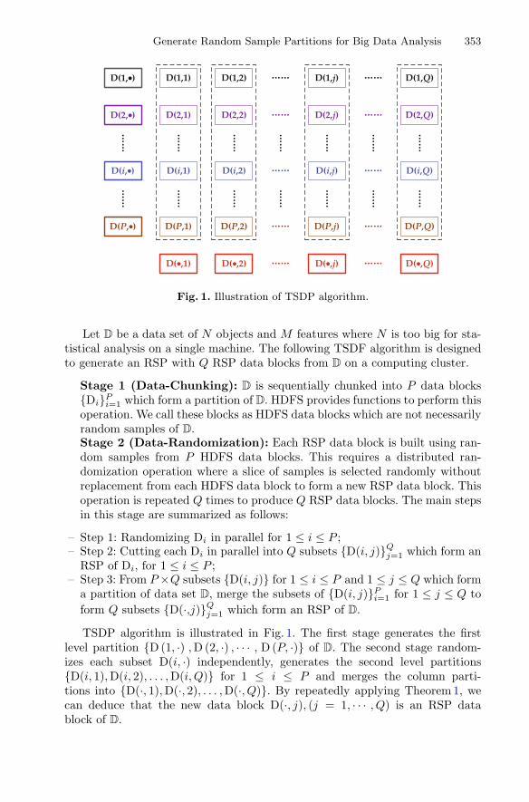
Generate Random Sample Partitions for Big Data Analysis 353
Fig. 1. Illustration of TSDP algorithm.
Let D be a data set of N objects and M features where N is too big for sta-tistical analysis on a single machine. The following TSDF algorithm is designedto generate an RSP with Q RSP data blocks from D on a computing cluster.
Stage 1 (Data-Chunking): D is sequentially chunked into P data blocks{Di}Pi=1 which form a partition of D. HDFS provides functions to perform thisoperation. We call these blocks as HDFS data blocks which are not necessarilyrandom samples of D.Stage 2 (Data-Randomization): Each RSP data block is built using ran-dom samples from P HDFS data blocks. This requires a distributed ran-domization operation where a slice of samples is selected randomly withoutreplacement from each HDFS data block to form a new RSP data block. Thisoperation is repeated Q times to produce Q RSP data blocks. The main stepsin this stage are summarized as follows:
– Step 1: Randomizing Di in parallel for 1 ≤ i ≤ P ;– Step 2: Cutting each Di in parallel into Q subsets {D(i, j)}Qj=1 which form an
RSP of Di, for 1 ≤ i ≤ P ;– Step 3: From P ×Q subsets {D(i, j)} for 1 ≤ i ≤ P and 1 ≤ j ≤ Q which form
a partition of data set D, merge the subsets of {D(i, j)}Pi=1 for 1 ≤ j ≤ Q toform Q subsets {D(·,j)}Qj=1 which form an RSP of D.
TSDP algorithm is illustrated in Fig. 1. The first stage generates the firstlevel partition {D (1, ·) ,D (2, ·) , · · · , D (P, ·)} of D. The second stage random-izes each subset D(i, ·) independently, generates the second level partitions{D(i, 1),D(i, 2), . . . ,D(i, Q)} for 1 ≤ i ≤ P and merges the column parti-tions into {D(·, 1),D(·, 2), . . . ,D(·, Q)}. By repeatedly applying Theorem1, wecan deduce that the new data block D(·, j), (j = 1, · · · , Q) is an RSP datablock of D.

354 C. Wei et al.
4 TSDP Implementation on Apache Spark
In this section, we present an implementation of the TSDP algorithm on ApacheSpark with HDFS. This implementation is called the round-random partitionerwhich is a hybrid between the range partitioner and the hash partitioner inSpark. Algorithm 1 shows the Pseudocode of this TSDP implementation in whichthe two stages are fulfilled as follows:
Algorithm 1. Round-Random PartitionerInput:- DHDFS : The HDFS file of a big data set D;- P : the number of RDD partitions in DHDFS ;- Q: the number of RSP data blocks in the RSP output HDFS file;Method:DRDD ← read DHDFS ; load HDFS file into an RDDfor all block i in DRDD do
K = Seq (1 to n)shuffle K;
end forbind K with DRDD partitions to generate pairRDD(K, V );repartition pairRDD using HashPartitioner(Q)DHDFS−RSP = values of pairRDD; ignore the random numbers in DHDFS−RSP
Output:- DHDFS−RSP : the final RSP; Generate the RSP HDFS file.
Stage 1 (Data-Chunking): This stage is performed using HDFS. A givenbig data set D is converted to an HDFS file with P HDFS data blocks. TheHDFS file of D is loaded to a Spark RDD using SparkContext.textFile()function. By default, each HDFS data block is mapped into an RDD partitionand the Spark RDD consists of P RDD partitions. The number of RDDpartitions to be generated can also be specified in the Spark data loadingfunction. This step is basically a range partitioner which produces P HDFSdata blocks2.Stage 2 (Data-Randomization): This stage randomizes all Spark parti-tions in parallel, randomly takes samples from each partition to form a set ofQ RDD partitions and saves these RDD partitions as RSP data blocks in anHDFS file. This stage is completed with the following operations:
– Key generation: Generate an array of a sequence of integers Ki (1 ≤ i ≤ P )for each RDD partition. The length of the sequence equals to the number ofrecords in the RDD partition. This operation is carried out in parallel.
2 Note: In Spark’s terminology, an RDD is equal to a partition of the big data set. Apartition is equal to a data block of the big data set. In this section, we use partitionto indicate a data block of the big data set loaded to an Spark RDD in order to beconsistent with Spark’ terminology in this Spark implementation.

Generate Random Sample Partitions for Big Data Analysis 355
– Key Randomizing and Binding: Use Spark shuffle operation to randomize theinteger sequences in the arrays Ks in parallel. Use the randomized integersin each array as random numbers and bind them to its corresponding RDDpartition in a Spark partition pair named as pairRDD.
– Repartitioning: Repartition the pair RDD by hashing the random numbersin the pairRDD to generate Q new RDD partitions in the pairRDD.
– RSP HDFS file generation: Ignore the random numbers in the pairRDD andsave the rest partitions as RSP data blocks in an HDFS file. This HDFS fileis an RSP representation of the big data set D.
Algorithm 2. Synthetic Data GenerationInput:- M : number of features;- P : number of data blocks;- N : number of objects;- H: number of clusters;Method:for all h = 1 to H do in parallel
μ(M) =Fill (μm)|μm ∈ U [0, 10]σ(M) =Fill (σm)|σm ∈ U (0, 1)D RDD ← GenerateRandomRDD(N/H, M, P, μ, σ)save D RDD on HDFS
end forCollect all files under one directory using HDFS APIs
5 Experiments and Results
In this section, we demonstrate the performance of Spark implementation of theTSDP algorithm on a computing cluster consisting of 2 name nodes and 27 datanodes, all running Centos 6.8. Each node has 16 cores (32 with Hyper-threading),128 GB RAM and 1.1 TB disk storage. Several synthetic data sets were used inthe experiments. We first present the method used to generate synthetic datasets. Then, we present the time performance of the algorithm in generating RSPdata blocks from HDFS data sets of different sizes, and the time performancein generating different numbers of RSP data blocks from 1 terabyte HDFS dataset in 1000 HDFS data blocks, and the time performance in generating thesame number of RSP data blocks from 1 terabyte HDFS data set with differentnumbers of HDFS data blocks. After that, we illustrate the changes of probabilitydistributions of HDFS data blocks and RSP data blocks. Finally, we use a realdata example to show how the RSP data blocks are used to build ensemblemodels from only few RSP data blocks with accuracies equivalent to or evenbetter than the model built from the entire data set.

356 C. Wei et al.
5.1 Synthetic Data Generation
Different synthetic data sets with different numbers of objects N , different num-bers of features M and different numbers of clusters H were generated and savedas HDFS files with different numbers of data blocks P . The clusters in the datasets have normal distributions with different means μ and standard deviations σ.Table 1 shows the characteristics of the synthetic data sets. The data generationalgorithm is illustrated in Algorithm2 which was implemented in Apache Spark.The data generation is performed in the following steps:
– Mean Generation: For each cluster, create a mean array for all featuresμ(M) and fill the array with values generated from the uniform distributionU (0, 10).
– Standard Deviation Generation: For each cluster, create a standard deviationarray for all features σ(M) and fill this array with values generated from thecontinuous uniform distribution U (0, 10).
– Cluster RDD Generation: Randomly generate a cluster RDD, D RDD, foreach cluster from the normal distribution with the following parameters,the number of objects N
H , the number of features M , the number of datablocks P , the array of features’ means μ, and the array of features’ standarddeviations σ.
– Save and Collect: Save D RDD on HDFS. After saving the RDDs for allclusters, they are collected under the same directory using HDFS APIs.
Table 1. Characteristics of synthetic data sets: N , M and H are the numbers ofobjects, features and clusters, respectively.
DS name Total size N M H Associated tasks
DS001 �100 GB 100,000,000 100 100 Classification
DS002 �200 GB 200,000,000 100 100 Classification
DS003 �300 GB 300,000,000 100 100 Classification
DS004 �400 GB 400,000,000 100 100 Classification
DS005 �500 GB 500,000,000 100 100 Classification
DS006 �600 GB 600,000,000 100 100 Classification
DS007 �700 GB 700,000,000 100 100 Classification
DS008 �800 GB 800,000,000 100 100 Classification
DS009 �900 GB 900,000,000 100 100 Classification
DS010 �1 TB 1,000,000,000 100 100 Classification
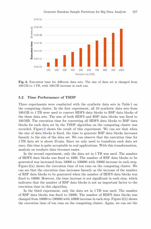
Generate Random Sample Partitions for Big Data Analysis 357
Fig. 2. Execution time for different data sets. The size of data set is changed from100GB to 1TB, with 100 GB increase in each run.
5.2 Time Performance of TSDP
Three experiments were conducted with the synthetic data sets in Table 1 onthe computing cluster. In the first experiment, all 10 synthetic data sets from100 GB to 1 TB were used to convert HDFS data blocks to RSP data blocks ofthe these data sets. The size of both HDFS and RSP data blocks was fixed to100 MB. The execution time for converting all HDFS data blocks to RSP datablocks for each data set by the TSDP algorithm on the computing cluster wasrecorded. Figure 2 shows the result of this experiment. We can see that whenthe size of data blocks is fixed, the time to generate RSP data blocks increaseslinearly to the size of the data set. We can observe that the execution time for1 TB data set is about 35 min. Since we only need to transform each data setonce, this time is quite acceptable in real applications. With this transformation,analysis on terabyte data becomes easier.
In the second experiment, only the data set in 1 TB was used. The numberof HDFS data blocks was fixed to 1000. The number of RSP data blocks to begenerated was increased from 10000 to 100000 with 10000 increase in each step.Figure 3(a) shows the execution time of ten runs on the computing cluster. Wecan see that the execution time increases linearly as the increase of the numberof RSP data blocks to be generated when the number of HDFS data blocks wasfixed to 10000. However, the time increase is not significant in each step, whichindicates that the number of RSP data blocks is not an important factor to theexecution time in this algorithm.
In the third experiment, only the data set in 1 TB was used. The numberof RSP data blocks was fixed to 10000. The number of HDFS data blocks waschanged from 10000 to 100000 with 10000 increase in each step. Figure 3(b) showsthe execution time of ten runs on the computing cluster. Again, we can see the

358 C. Wei et al.
linear increase in execution time as increase in the number of HDFS data blocksin the HDFS file. However, the increase is more significant in each step. Thisindicates that the number of HDFS blocks in the HDFS file is an important factorto the execution time of this algorithm. We can see that converting 1 terabyteHDFS data set with 10000 HDFS blocks to 10000 RSP data blocks took about30 min where converting the same data with 100000 HDFS blocks to 10000 RSPdata blocks took more than 1 h. The reason is that the HDFS data blocks needto be randomized in this algorithm, which requires more memory resource toexecute in parallel when the size and number of HDFS data block become large.These three experiments show that the TSDP algorithm is scalable to terabytedata, which facilitates the analysis of big data in terabyte size.
5.3 Distribution of Data Blocks
In this section, we show the probability distributions of features in HDFS datablocks and RSP data blocks and demonstrate that RSP data blocks of the samedata set have similar probability distributions among themselves whereas theHDFS data blocks do not have similar probability distributions among them-selves. Given a sequence of values of one feature from an HDFS data block, theprobability density function (p.d.f.) is represented as a kernel density functionwhich can be estimated by Parzen window method [14]. The density estima-tion algorithm is used to disperse the mass of the empirical p.d.f. over a regulargrid with at least 512 points. The fast Fourier transform is used to convolve theapproximation with a discredited version of the kernel. Gaussian basis functionsare used to approximate univariate data. The rule-of-thumb is used to determinethe bandwidth h of Parzen window [14] as
h =(
4σ5
3n
)1/5
≈ 1.06σn−1/5 (2)
where σ is the standard deviation of the feature and n is the number of points.With this method, we plot the p.d.f. of any continuous feature in an HDFS datablock and an RSP data block.
Figure 4(a) and (c) show the p.d.f. of two features from 6 randomly chosenHDFS data blocks in data set DS010. We can see that different HDFS datablocks have different probability distributions of two features. This indicatesthat these data blocks cannot be used to estimate and analyze the big data setbecause they are not representatives of the entire data set. To analyze the bigdata set, all HDFS data blocks must be taken into consideration, therefore, alldata blocks have to be loaded to memory and compute. If the computing clusterhas limited resource, then, the ability of analyzing big data will be limited.
Figure 4(b) and (d) show the p.d.f. of two features from 6 randomly cho-sen RSP data blocks in data set DS010. We can see that all RSP blocks havethe same probability distribution on the same feature. Theorem1 shows thatthe expectation of the probability distribution of each RSP data block is theprobability distribution of the entire data set. Therefore, these RSP data blocks
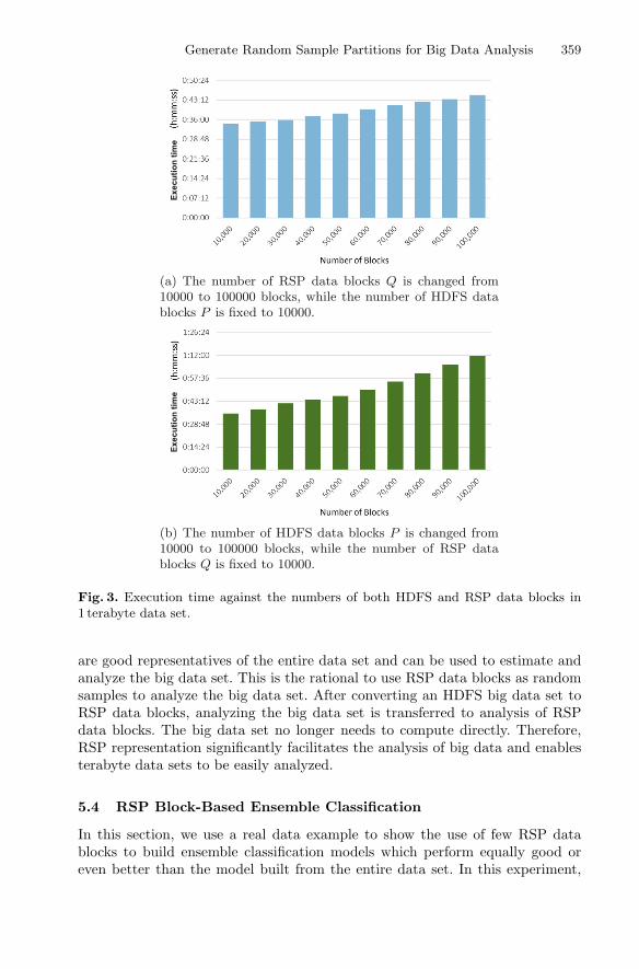
Generate Random Sample Partitions for Big Data Analysis 359
Fig. 3. Execution time against the numbers of both HDFS and RSP data blocks in1 terabyte data set.
are good representatives of the entire data set and can be used to estimate andanalyze the big data set. This is the rational to use RSP data blocks as randomsamples to analyze the big data set. After converting an HDFS big data set toRSP data blocks, analyzing the big data set is transferred to analysis of RSPdata blocks. The big data set no longer needs to compute directly. Therefore,RSP representation significantly facilitates the analysis of big data and enablesterabyte data sets to be easily analyzed.
5.4 RSP Block-Based Ensemble Classification
In this section, we use a real data example to show the use of few RSP datablocks to build ensemble classification models which perform equally good oreven better than the model built from the entire data set. In this experiment,

360 C. Wei et al.
we used the asymptotic ensemble framework (called Alpha framework) [10] tobuild ensemble models from RSP data blocks.
Fig. 4. p.d.f. comparison between HDFS data blocks and RSP data blocks in 1TBsynthetic data.
Alpha framework is illustrated in Fig. 5. A big data set D is first convertedinto RSP data blocks using the TSDP algorithm. Then, a subset of RSP datablocks is randomly selected without replacement, e.g., D5,D120,D506 and D890
in Fig. 5. After that, a base model is built from each of these data blocks, e.g.,four classifiers π1, π2, π3, π4 built in parallel from 4 selected RSP data blocks.The next operation is to update the ensemble model Π with the newly builtclassifiers and evaluate Π. If Π satisfies the termination condition(s), then outputΠ, otherwise, go back to RSP representation and randomly select a new batch ofRSP data blocks to build a second batch of new classifiers, update the ensemble

Generate Random Sample Partitions for Big Data Analysis 361
model Π with the second batch of classifiers and evaluate it again. This processcontinues until a satisfactory ensemble model Π is obtained or all RSP datablocks are used up.
Fig. 5. Alpha framework: an asymptotic ensemble framework to build ensemble modelsfrom RSP data blocks.
The real data HIGGS with N = 11, 000, 000 objects and M = 28 features wasused in this experiment. 400 RSP data blocks were generated with the TSDPalgorithm. Figure 6(a) shows the accuracy of the ensemble models after eachbatch of data blocks. We can see that there is no significant change after usingabout 15% of the data and the accuracy value converges to a value which isapproximately the same as the accuracy of a single model built from the wholedata set (the dotted line in the figure). In addition, we also used the 100 GBsynthetic data set DS001 to test the performance of the ensemble models fromRSP data blocks. We found that only 10% of this data is enough to build anensemble model with 90% accuracy as shown in Fig. 6(b). In such cases, we donot need to continue building further models from the remaining data blocks.
6 Discussions
Two computational costs are significant in cluster computing: one is the costof communications among the computing nodes and the other is the cost ofi/o operations on read/write data from/to the disks of local nodes. The twocosts limit the ability of cluster computing on analysis of big data with complex
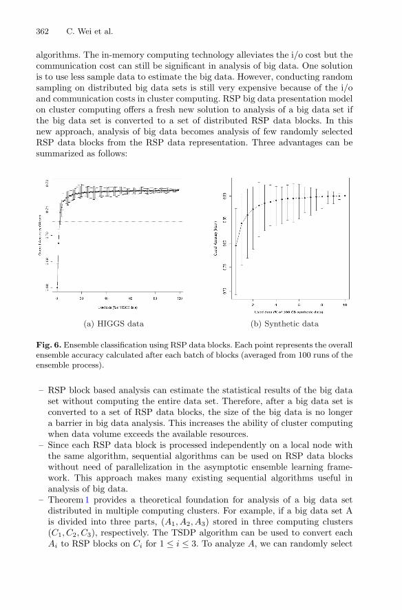
362 C. Wei et al.
algorithms. The in-memory computing technology alleviates the i/o cost but thecommunication cost can still be significant in analysis of big data. One solutionis to use less sample data to estimate the big data. However, conducting randomsampling on distributed big data sets is still very expensive because of the i/oand communication costs in cluster computing. RSP big data presentation modelon cluster computing offers a fresh new solution to analysis of a big data set ifthe big data set is converted to a set of distributed RSP data blocks. In thisnew approach, analysis of big data becomes analysis of few randomly selectedRSP data blocks from the RSP data representation. Three advantages can besummarized as follows:
(a) HIGGS data (b) Synthetic data
Fig. 6. Ensemble classification using RSP data blocks. Each point represents the overallensemble accuracy calculated after each batch of blocks (averaged from 100 runs of theensemble process).
– RSP block based analysis can estimate the statistical results of the big dataset without computing the entire data set. Therefore, after a big data set isconverted to a set of RSP data blocks, the size of the big data is no longera barrier in big data analysis. This increases the ability of cluster computingwhen data volume exceeds the available resources.
– Since each RSP data block is processed independently on a local node withthe same algorithm, sequential algorithms can be used on RSP data blockswithout need of parallelization in the asymptotic ensemble learning frame-work. This approach makes many existing sequential algorithms useful inanalysis of big data.
– Theorem 1 provides a theoretical foundation for analysis of a big data setdistributed in multiple computing clusters. For example, if a big data set Ais divided into three parts, (A1, A2, A3) stored in three computing clusters(C1, C2, C3), respectively. The TSDP algorithm can be used to convert eachAi to RSP blocks on Ci for 1 ≤ i ≤ 3. To analyze A, we can randomly select

Generate Random Sample Partitions for Big Data Analysis 363
the same number of RSP data blocks from each computing cluster and mergethe three sets of RSP data blocks into one set of RSP data blocks for A whereeach new RSP block is formed by merging three RSP blocks, each from onecomputing cluster. According to Theorem 1, the new blocks are RSP datablocks of A and can be used to estimate the statistical properties of A orbuild ensemble models for A. This new approach provides an opportunity toanalyze big data sets cross data centers. However, detail technology needs tobe further developed to facilitate analysis of big data sets cross multiple datacenters.
7 Conclusions and Future Work
In this paper, we have proposed a two-stage data processing (TSDP) algorithm togenerate the random sample partitions (RSPs) from HDFS big data sets for bigdata analysis. This algorithm is an enabling technology for RSP data block basedanalysis of big data sets, which does not need to compute the entire big data set.We have presented an implementation of the TSDP algorithm on Apache Sparkand demonstrated the time performance of this algorithm on 1 terabyte data.The experiment results show that conversion of an HDFS data set in 1 terabytewas completed in less one hour which is well acceptable in real applications. Wehave also shown a real data example to demonstrate that the ensemble modelsbuilt using few RSP data blocks performed better than the model built from theentire data set. Our future work is to extend the current algorithm to work onbigger data sets, e.g., 10 terabytes. We will also develop a distributed big datamanagement system on computing clusters based on the RSP representationmodel.
References
1. Fan, J., Fang, H., Han, L.: Challenges of big data analysis. Nat. Sci. Rev. 1(2),293–314 (2014)
2. Zhao, J., Zhang, W., Liu, Y.: Improved K-means cluster algorithm in telecommu-nications enterprises customer segmentation. In: IEEE International Conferenceon Information Theory and Information Security, pp. 167–169 (2010)
3. Michael, B.: Uncovering online political communities of Belgian MPs through socialnetwork clustering analysis. In Proceedings of the ACM 2015 2nd InternationalConference on Electronic Governance and Open Society, pp. 150–163 (2015)
4. Ahmad, A., Paul, A., Rathore, M.M.: An efficient divide-and-conquer approachfor big data analytics in machine-to-machine communication. Neurocomputing174(86), 439–453 (2016)
5. Shvachko, K., Kuang, H., Radia, S., Chansler, R.: The hadoop distributed filesystem. In: IEEE 26th Symposium Mass Storage Systems and Technologies, pp.1–10 (2010)
6. Dean, J., Ghemawat, S.: MapReduce: simplified data processing on large clusters.Commun. ACM 51(1), 107–113 (2008)

364 C. Wei et al.
7. Elteir, M., Lin, H., Feng, W.C.: Enhancing mapreduce via asynchronous data pro-cessing. In: IEEE International Conference on Parallel and Distributed Systems,pp. 397–405 (2010)
8. Zaharia, M., Chowdhury, M., Franklin, M.J., Shenker, S., Stoica, I.: Spark: clustercomputing with working sets. In: HotCloud 2010, p. 10 (2010)
9. Salloum, S., Dautov, R., Chen, X., Peng, P.X., Huang, J.Z.: Big data analytics onapache spark. Int. J. Data Sci. Anal. 1(3–4), 145–164 (2016)
10. Salloum, S., Huang, J.Z., He, Y.L.: Empirical analysis of asymptotic ensemblelearning for big data. In: Proceedings of the 2016 IEEE/ACM International Con-ference on Big Data Computing, Applications and Technologies, pp. 8–17 (2016)
11. Cormode, G., Duffield, N.: Sampling for big data: a tutorial. In: Proceedings of the20th ACM SIGKDD International Conference on Knowledge Discovery and DataMining, p. 1975 (2014)
12. Garcia, D., Lubiano, M.A., Alonso, M.C.: Estimating the expected value of fuzzyrandom variables in the stratified random sampling from finite populations. Inf.Sci. 138(4), 165–184 (2001)
13. Leo, S., Zanetti, G.: Pydoop: a python mapreduce and HDFS API for hadoop.In: Proceedings of the 19th ACM International Symposium on High PerformanceDistributed Computing, pp. 819–825 (2010)
14. Sheather, S.J., Jones, M.C.: A reliable data-based bandwidth selection method forkernel density estimation. J. Roy. Stat. Soc. 53(3), 683–690 (1991)

An Improved Measurement of the ImbalancedDataset
Chunkai Zhang1(&), Ying Zhou1, Yingyang Chen1, Changqing Qi1,Xuan Wang1, and Lifeng Dong2
1 Harbin Institute of Technology Shenzhen Graduate School, Shenzhen, [email protected]
2 Hamline University, 1536 Hewitt Avenue, St. Paul, USA
Abstract. Imbalanced classification is a classification problem that violates theassumption of uniform distribution of samples. In such problems, traditionalimbalanced datasets are measured in terms of the imbalance of sample size,without considering the distribution information, which has a more importantimpact on the classification performance, so the traditional measurements have aweak relation with the classification performance. This paper proposed animproved measurement for imbalanced datasets, it is based on the idea that asample surrounded by more same class samples is easier to classify, for eachsample of different classes, the proposed method calculates the average numberof the k nearest neighbors in the same class in different subsets under theweighted k-NN, after that, the product of these average values is regarded as themeasurement of this dataset, and it is a good indicator of the relationshipbetween the distribution of samples and the classification results. The experi-mental results show that the proposed measurement has a higher correlation withthe classification results and shows the difficulty of classification of data setsmore clearly.
Keywords: Imbalanced classification � Measurement � Imbalance ratio
1 Introduction
The classification problem is a very important part of machine learning. In the tradi-tional classification problem, the model training is based on the assumption that thesample distribution is uniform, so the classification cost of each sample is consistent.However, in realistic data sets, the assumption of uniform distribution of samples isdifficult to satisfy, in order to pursue the global accuracy, the traditional classifier caneasily get an unsatisfying classification performance of the minority samples, causingthem to be hard to recognize. The imbalanced classification problem has appeared inmany fields, such as bioinformatics [1, 2], remote sensing image recognition [3], andprivacy protection in cybersecurity [4–6]. The wide coverage of the imbalance problemhas very important practical significance.
The traditional imbalanced classification problem has two features: the difference insample size; the difference in misclassification cost for different classes. Scholars haveproposed the data-level methods for feature 1 and the algorithm-level methods for
© Springer International Publishing AG, part of Springer Nature 2018M. Luo and L.-J. Zhang (Eds.): CLOUD 2018, LNCS 10967, pp. 365–376, 2018.https://doi.org/10.1007/978-3-319-94295-7_25
feature 2. As the data-level methods can be regarded as a preprocessing before trainingthe classifier, so they have been popular for many years. The data-level methods can bedivided into the oversampling to add the minority samples, the under-sampling toreduce the majority samples and the hybrid sampling methods, they aim to get abalanced dataset, which is defined by the imbalanced dataset measurement.
Measurement of the imbalanced datasets can be divided into two types: localmeasurements and global measurements. The local measurements refer to thesemethods which need traversing each sample in a data set [7, 8], calculating a mea-surement usually accompanied by the k-NN algorithm for each sample, the overallmeasurement is defined by the mean value of measurement of all the samples in thedataset. Because this kind of measurement contains the calculation for each sample,and it can be used in the sampling algorithm to find a simpler dataset to model withenough information with the original dataset. Global measurement [9] refers to a resultcalculated for a sample in the entire data set, or a variety of indicators derived fromstatistical analysis. It is usually accompanied by a variety of calculations for the sep-arate results of the positive and negative subsets. Such measurements are difficult toachieve in a single implemented on the sample, it can only be used as a measure of thedataset, and it is difficult to play a role in the sampling algorithm because the movementof a single sample can hardly affect the original measurement result.
As the number of samples has had a noticeable effect on the classification results.Therefore, the imbalance ratio [8–10] (IR) of the number of samples in different classeshas been popular for many years as a measurement of imbalanced datasets. Based onIR, scholars have proposed many sampling algorithms to balance the datasets to releaseeffect of the imbalance in sample size on the classification performance, so the mea-surement plays a very important role in imbalanced classification. However, the IR isnot informative enough to measure a specific dataset overall, as it is a global mea-surement, studies [10] have shown that when the number of samples is relatively large,it does not cause a reduction in the classification performance of the minority class, butwhen the number of samples is seriously insufficient, the rarity of the minority sampleswill cause a low recognition rate of the minority samples. The local measurementsdevelop the global ones as they take the distribution into consideration, meanwhile,with the understanding of the classifier and data, the distribution based samplingmethods [12–14] are taking the distribution information into consideration, and alsoencourage the new measurements to contain the distribution information.
This paper proposes a measurement containing the distribution information, it ismotivated that the nearer a sample is with the same labeled samples, the easier it can beclassified correctly. The proposed method calculates the average number of the knearest neighbors in the same class in different subsets under the weighted k-NN, afterthat, the product of these average values is regarded as the measurement of this dataset.It improves the correlation between the measurement and the final classification per-formance, which indicate that the proposed is more informative. This paper is arrangedas follows: Sect. 2 describes the related work in measurement of the imbalanceddataset, Sect. 3 shows the proposed measurement improved generalized imbalancedratio (IGIR), and Sect. 4 describes the experimental results and analysis, the finalsection concludes the proposed method and the future work.
366 C. Zhang et al.

2 Related Work
There are many different factors which have effects on the imbalanced classification,resulting in various kinds of measurements considering different factors. For example,the Imbalance Ratio (IR) is based on the difference in sample size, the maximumFisher’s discriminant ratio (F1) is based on the overlap in feature values from differentclasses, and the Complexity Measurement (CM), Generalized Imbalance Ratio (GIR),and the proposed method Improved Generalized Imbalance Ratio (IGIR) are based onthe idea that data distribution plays important role in imbalanced classification. Thesemeasurements are used in such two ways: indicate whether a dataset is easy to classify,and measure the sampled subset in sampling methods. Therefore, in order to achieve abetter performance, the measurement should have a relatively high correlation with theclassification results.
Given dataset X, which contains N+ positive samples (the minority class), N_negative samples (the majority class), and the total number of samples is N = N_ + N+.
2.1 IR
Imbalance ratio [11–13] the definition is as follows, it is defined as the size sampleratio:
IR ¼ NNþ
ð1Þ
When samples with different labels have the same distribution, the sample size isable to reflect whether the samples are easy to classify, otherwise, the IR is not soinformative to indicate whether the dataset is easy to classify. For example, in theFig. 1, the IR of data in (a) is 4 and in (b) is 1, but the two classes in (a) have a clearlinear boundary while there is not in (b), so we can get 100% accuracy in (a) but cannotin (b) with a same linear model, which is contrary to the comparison result of IR, sinceIR is the proportion of sample size and does not contain any sample distributioninformation, complexity of the data distribution cannot be represented in IR.
Fig. 1. The dilemma of IR.
An Improved Measurement of the Imbalanced Dataset 367

2.2 F1
A classical measure of the discriminative power of the covariates, or features, isFisher’s discriminant ratio [9], and F1 is the maximum Fishers discriminant ratio:
f ¼ l1 � l2ð Þ2r21 þ r22
ð2Þ
Where l1, l2, r12, r2
2 are the means and variances of the positive and negativesubsets, respectively. For multidimensional problems, the maximum f over all featurescan be used. However, if f gets 0, it does not necessarily mean that the classes are notseparable, as it could just be that the separating boundary is not parallel to an axis inany of the given features.
2.3 CM
CM [7] focuses on the local information for each data point via the nearest neighbors,and uses this information to capture data complexity.
CMk jð Þ ¼ I
Number of patternsj0in Nj with y0j ¼ yj
k� 0:5
0BB@
1CCA ð3Þ
Where I(.) is the indicator function. The overall measurement is
CMk ¼ 1n
Xn
j¼1CMk jð Þ ð4Þ
CM is determined by the label of its neighbors. If the neighbors of a sample containmore samples in the same class, the sample will be easier to classify. On the contrary, ifthe samples are surrounded by samples with different labels, then the sample is difficultto classify correctly, and the average number of different classes samples contained inthe k nearest neighbors is used as the measurement. The higher the CM, the moredifficult the dataset is to learn.
2.4 GIR
The GIR [8] is an improvement of cm, it focuses on the differences in the difficulty ofclassifying the samples in different classes. A dataset with a larger GIR is more difficultto get a good performance of the minority class, as the classifier tends to be trained withthe easier samples according to the Occam shaver principle. Because we tend to use amost simple classifier to fit the whole dataset, while the more difficult samples need amore complex classifier, which may cause overfitting with single classifier, so this isthe reason why ensemble can be effective in the imbalance classification, as they have
368 C. Zhang et al.

the different classifiers corresponding to different levels of sample classificationdifficulty.
Tþ ¼ 1Nþ
Xx2P
1k
Xk
r¼1IR x;Xð Þ ¼ 1
Nþ
Xx2P tk xð Þ ð5Þ
T� ¼ 1N�
Xx2N tk xð Þ ð6Þ
GIR ¼ T� � Tþ ð7Þ
Where IR(x, X) is an indicator function. For a sample x, if its k-nearest neighbor’slabel is the same as x, the result is 1, otherwise, it gets 0.
GIR considers the different measurements of the positive and negative subsets,which is an improvement of CM, GIR is defined as the difference between positive andnegative sample subsets, and paper [8] successfully applies GIR to oversampling andunder-sampling algorithms. The experimental results show that GIR-based resamplingalgorithm can effectively improve the classification performance.
However, there are two problems in GIR, first, in the classification process, besidesthe label of k nearest neighbors, their distance from the sample will also affect theclassification result. Second, the GIR of the data set is calculated by the measurementof the negative class minus positive class, so GIR is a relative measurement. As shownin Table 1, the final result shows that the two data sets have the same GIR, but it isclear that the dataset (b) is more difficult to classify than (a). Therefore, GIR is not sosufficient to fully interpret the complexity of the dataset distribution.
3 The Proposed Method
We proposed an improved measurement called IGIR in this paper, it is based on theidea that the sample distribution plays an important role in the classification result, themotivation of IGIR is that if there are many samples with the same label around thesample, the sample is easily classified, and on the contrary, the sample is hard toclassify. Different distances of the k nearest neighbors have different effects on theclassification results of the sample.
weightr ¼ k � rk
; r ¼ 0; 1; 2 � � � k � 1 ð8Þ
Table 1. The dilemma of GIR
(a) (b)
T− 0.9 0.5T+ 0.7 0.3GIR 0.2 0.2
An Improved Measurement of the Imbalanced Dataset 369

wei-Tþ ¼ 1Nþ
Xx2P 1=k
Xk
r¼1weightr � IRðx;XÞ ¼ 1
Nþ
Xx2P tkðxÞ ð9Þ
wei-T� ¼ 1N�
Xx2N tkðx) ð10Þ
wei-IGIR ¼ffiffiffiffiffiffiffiffiffiffiffiffiffiffiffiffiffiffiffiffiffiffiffiffiffiffiffiffiffiffiffiffiffiffiwei-T� � wei-Tþ
pð11Þ
In the calculation of IGIR, the k-nearest neighbors of each sample in the dataset arecalculated at first, and their neighboring class labels are retained. First, according to thecalculation method in formula (8), the weights of the k nearest neighbors are graduallyreduced to 0. The main reason for not using distance is that the distances betweendifferent samples and its neighbors are inconsistent. This will result in the inconsistencyof the weights of each sample in the calculation process, therefore, it is not possible tohave a comparative standard for the overall results; second, to describe the datasetreasonably with an absolute measurement, and to avoid the relativity in the originalGIR and spired by the definition of geometric mean, IGIR is defined as the compoundmeasurements of positive and negative subsets. In this case, to ensure that the order ofmagnitude is unchanged, it is processed by prescribing to better measure the difficultyof classification of the dataset.
In the proposed method, firstly, calculate the weight according to formula (8),secondly, compute the k nearest neighbors of each sample and tk xð Þ for each sample,thirdly, compute the average tk xð Þ of the positive and negative subsets, finally, computethe IGIR according to the formula (11).
IGIR can be regarded as the average classification accuracy under a weightedk-NN. That is, the more neighbors of the same class in the sample, the more likely thesample is to be classified as the original classifier, then IGIR has the nature to be relatedto the final classification performance.
370 C. Zhang et al.

4 Experimental Results
4.1 Datasets
The experimental data in this paper comes from the UCI machine learning database[14]. Some of them are multi-class datasets, in order to obtain a harder dataset toclassify, we select one of the class as the minority class, and the rest of classes areregarded as the majority, and the details are shown as Table 4.
4.2 Evaluation
In the binary imbalanced classification, the confusion matrix is often used to evaluatethe performance of the classifier, which is defined in Table 2:
FN represents the number of positive samples that are incorrectly classified asnegative, and FP is the number of samples that are incorrectly classified as positive,there have been compound evaluations, such as F-value and Gmean [15].
sensitivity ¼ TPTPþFP
ð12Þ
recall ¼ TPTPþFN
ð13Þ
F-value ¼ ð1þ b2Þ � recall� precision
b2 � recallþ precisionð14Þ
Gmean ¼ffiffiffiffiffiffiffiffiffiffiffiffiffiffiffiffiffiffiffiffiffiffiffiffiffiffiffiffiffiffiffiffiffiffiffiffiffiffiffiffi
TPTPþ FN
� TNTNþ FP
rð15Þ
4.3 Experimental Settings and Results
Set b = 1 in F-value called F1_min, all involved k-NN are set with k = 5, the classifieris C4.5, all results are the average of 10 times of 10-fold cross-validation.
Table 2. Confusion metrics
Positive prediction Negative prediction
Positive class True positive (TP) False negative (FN)Negative class False positive (FP) True negative (TN)
An Improved Measurement of the Imbalanced Dataset 371

Fig. 2. Measurements and sensitivity
372 C. Zhang et al.
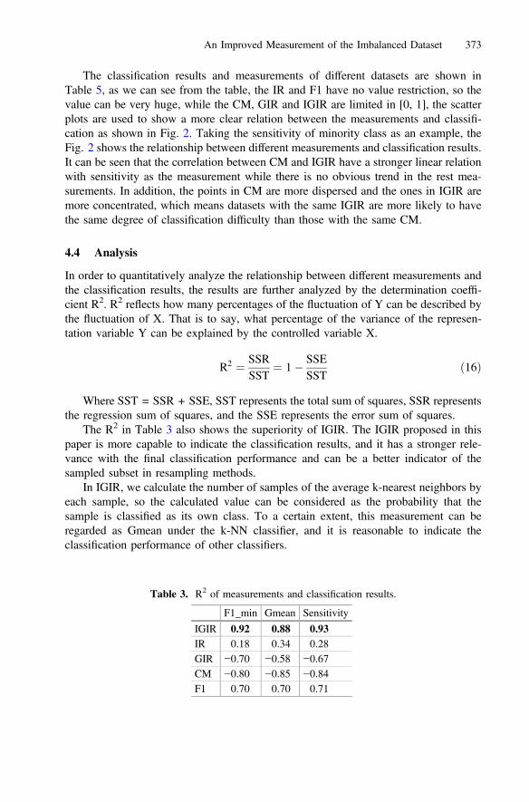
The classification results and measurements of different datasets are shown inTable 5, as we can see from the table, the IR and F1 have no value restriction, so thevalue can be very huge, while the CM, GIR and IGIR are limited in [0, 1], the scatterplots are used to show a more clear relation between the measurements and classifi-cation as shown in Fig. 2. Taking the sensitivity of minority class as an example, theFig. 2 shows the relationship between different measurements and classification results.It can be seen that the correlation between CM and IGIR have a stronger linear relationwith sensitivity as the measurement while there is no obvious trend in the rest mea-surements. In addition, the points in CM are more dispersed and the ones in IGIR aremore concentrated, which means datasets with the same IGIR are more likely to havethe same degree of classification difficulty than those with the same CM.
4.4 Analysis
In order to quantitatively analyze the relationship between different measurements andthe classification results, the results are further analyzed by the determination coeffi-cient R2. R2 reflects how many percentages of the fluctuation of Y can be described bythe fluctuation of X. That is to say, what percentage of the variance of the represen-tation variable Y can be explained by the controlled variable X.
R2 ¼ SSRSST
¼ 1� SSESST
ð16Þ
Where SST = SSR + SSE, SST represents the total sum of squares, SSR representsthe regression sum of squares, and the SSE represents the error sum of squares.
The R2 in Table 3 also shows the superiority of IGIR. The IGIR proposed in thispaper is more capable to indicate the classification results, and it has a stronger rele-vance with the final classification performance and can be a better indicator of thesampled subset in resampling methods.
In IGIR, we calculate the number of samples of the average k-nearest neighbors byeach sample, so the calculated value can be considered as the probability that thesample is classified as its own class. To a certain extent, this measurement can beregarded as Gmean under the k-NN classifier, and it is reasonable to indicate theclassification performance of other classifiers.
Table 3. R2 of measurements and classification results.
F1_min Gmean Sensitivity
IGIR 0.92 0.88 0.93IR 0.18 0.34 0.28GIR −0.70 −0.58 −0.67CM −0.80 −0.85 −0.84F1 0.70 0.70 0.71
An Improved Measurement of the Imbalanced Dataset 373
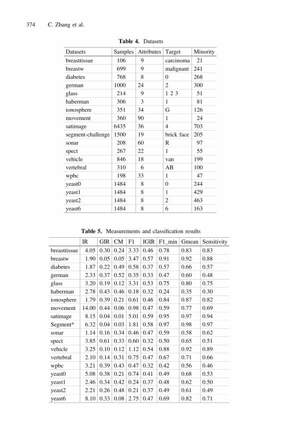
Table 4. Datasets
Datasets Samples Attributes Target Minority
breasttissue 106 9 carcinoma 21breastw 699 9 malignant 241diabetes 768 8 0 268german 1000 24 2 300glass 214 9 1 2 3 51haberman 306 3 1 81ionosphere 351 34 G 126movement 360 90 1 24satimage 6435 36 4 703segment-challenge 1500 19 brick face 205sonar 208 60 R 97spect 267 22 1 55vehicle 846 18 van 199vertebral 310 6 AB 100wpbc 198 33 1 47yeast0 1484 8 0 244yeast1 1484 8 1 429yeast2 1484 8 2 463yeast6 1484 8 6 163
Table 5. Measurements and classification results
IR GIR CM F1 IGIR F1_min Gmean Sensitivity
breasttissue 4.05 0.30 0.24 3.33 0.46 0.78 0.83 0.83breastw 1.90 0.05 0.05 3.47 0.57 0.91 0.92 0.88diabetes 1.87 0.22 0.49 0.58 0.37 0.57 0.66 0.57german 2.33 0.37 0.52 0.35 0.33 0.47 0.60 0.48glass 3.20 0.19 0.12 3.31 0.53 0.75 0.80 0.75haberman 2.78 0.43 0.46 0.18 0.32 0.24 0.35 0.30ionosphere 1.79 0.39 0.21 0.61 0.46 0.84 0.87 0.82movement 14.00 0.44 0.06 0.98 0.47 0.59 0.77 0.69satimage 8.15 0.04 0.01 5.01 0.59 0.95 0.97 0.94Segment* 6.32 0.04 0.03 1.81 0.58 0.97 0.98 0.97sonar 1.14 0.16 0.34 0.46 0.47 0.59 0.58 0.62spect 3.85 0.61 0.33 0.60 0.32 0.50 0.65 0.51vehicle 3.25 0.10 0.12 1.12 0.54 0.88 0.92 0.89vertebral 2.10 0.14 0.31 0.75 0.47 0.67 0.71 0.66wpbc 3.21 0.39 0.43 0.47 0.32 0.42 0.56 0.46yeast0 5.08 0.38 0.21 0.74 0.41 0.49 0.68 0.53yeast1 2.46 0.34 0.42 0.24 0.37 0.48 0.62 0.50yeast2 2.21 0.26 0.48 0.21 0.37 0.49 0.61 0.49yeast6 8.10 0.33 0.08 2.75 0.47 0.69 0.82 0.71
374 C. Zhang et al.

5 Conclusion
In this paper, an improved measurement for imbalanced datasets is proposed, it takesthe distribution information into consideration and it is based on the idea that a samplesurrounded by more same class samples is easier to classify, for each sample ofdifferent classes, the proposed method calculates the average number of the k nearestneighbors in the same class in different subsets under the weighted k-NN, after that, theproduct of these average values is regarded as the measurement of this dataset. Theexperimental results show that the proposed measurement has a higher correlation withthe classification results and can be used in the sampling algorithm. The future workwill be sampling algorithms based on this measurement to improve the classificationresults.
Acknowledgment. This study was supported by the Shenzhen Research Council (Grant No.JSGG20170822160842949, JCYJ20170307151518535, JCYJ20160226201453085, JCYJ20170307151831260).
References
1. Wang, Y., Li, X., Tao, B.: Improving classification of mature microRNA by solving classimbalance problem. Sci. Rep. 6, 25941 (2016)
2. Stegmayer, G., Yones, C., Kamenetzky, L., Milone, D.H.: High class-imbalance inpre-miRNA prediction: a novel approach based on deepSOM. IEEE/ACM Trans. Comput.Biol. Bioinf. 14(6), 1316–1326 (2017)
3. Leichtle, T., Geiß, C., Lakes, T., Taubenböck, H.: Class imbalance in unsupervised changedetection – a diagnostic analysis from urban remote sensing. Int. J. Appl. Earth Obs. Geoinf.60, 83–98 (2017)
4. Li, C., Liu, S.: A comparative study of the class imbalance problem in Twitter spamdetection. Concurr. Comput. Pract. Exp. 30(4) (2018)
5. Singh, S., Liu, Y., Ding, W., Li, Z.: Empirical evaluation of big data analytics using designof experiment: case studies on telecommunication data (2016)
6. Hale, M.L., Walter, C., Lin, J., Gamble, R.F.: A priori prediction of phishing victimizationbased on structural content factors (2017)
7. Anwar, N., Jones, G., Ganesh, S.: Measurement of data complexity for classificationproblems with unbalanced data. Stat. Anal. Data Min. 7(3), 194–211 (2014)
8. Tang, B., He, H.: GIR-based ensemble sampling approaches for imbalanced learning. PatternRecogn. 71, 306–319 (2017)
9. Ho, T.: A data complexity analysis of comparative advantages of decision forestconstructors. Pattern Anal. Appl. 5(2), 102–112 (2002)
10. Chawla, N.V., Bowyer, K.W., Hall, L.O., Kegelmeyer, W.P.: SMOTE: synthetic minorityover-sampling technique. J. Artif. Intell. Res. 16(1), 321–357 (2002)
11. Han, H., Wang, W.-Y., Mao, B.-H.: Borderline-SMOTE: a new over-sampling method inimbalanced data sets learning. In: Huang, D.-S., Zhang, X.-P., Huang, G.-B. (eds.) ICIC2005. LNCS, vol. 3644, pp. 878–887. Springer, Heidelberg (2005). https://doi.org/10.1007/11538059_91
12. Zhang, M.: Foundations of Modern Analysis. Academic Press, London (1960)
An Improved Measurement of the Imbalanced Dataset 375

13. Weiss, G.M.: Learning with rare cases and small disjuncts. In: Twelfth InternationalConference on Machine Learning, pp. 558–565 (1995)
14. Zhang, H., Wang, Z.: A normal distribution-based over-sampling approach to imbalanceddata classification. In: International Conference on Advanced Data Mining and Applications,pp. 83–96 (2011)
15. Li, D.C., Hu, S.C., Lin, L.S., Yeh, C.W.: Detecting representative data and generatingsynthetic samples to improve learning accuracy with imbalanced data sets. PLoS ONE 12(8),e0181853 (2017)
16. Moreo, A., Esuli, A., Sebastiani, F.: Distributional random oversampling for imbalanced textclassification, pp. 805–808 (2016)
17. Amini, M.R., Usunier, N., Goutte, C.: http://archive.ics.uci.edu/ml/datasets.html. Accessed22 Mar 2018
18. Menardi, G., Torelli, N.: Training and assessing classification rules with imbalanced data.Data Min. Knowl. Disc. 28(1), 92–122 (2014)
376 C. Zhang et al.

A Big Data Analytical Approachto Cloud Intrusion Detection
Halim Gorkem Gulmez, Emrah Tuncel, and Pelin Angin(B)
Department of Computer Engineering, Middle East Technical University,Ankara, Turkey
{gorkem.gulmez,emrah.tuncel}@metu.edu.tr, [email protected]
Abstract. Advances in cloud computing in the past decade have madeit a feasible option for the high performance computing and mass stor-age needs of many enterprises due to the low startup and managementcosts. Due to this prevalent use, cloud systems have become hot tar-gets for attackers aiming to disrupt reliable operation of large enterprisesystems. The variety of attacks launched on cloud systems, includingzero-day attacks that these systems are not prepared for, call for a uni-fied approach for real-time detection and mitigation to provide increasedreliability. In this work, we propose a big data analytical approach tocloud intrusion detection, which aims to detect deviations from the nor-mal behavior of cloud systems in near real-time and introduce measuresto ensure reliable operation of the system by learning from the conse-quences of attack conditions. Initial experiments with recurrent neuralnetwork-based learning on a large network attack dataset demonstratethat the approach is promising to detect intrusions on cloud systems.
Keywords: Intrusion detection · Cloud · Recurrent neural networksBig data analytics
1 Introduction
Advances in the networking and virtualization technologies in the past decadehave made cloud platforms a popular choice for the data storage and computingneeds of many enterprises. Many companies have moved their infrastructuresto major cloud platforms for improved reliability. As cloud services have gottenpopular and common with decreased costs, they have also become hot targetsfor attacks. The rise of the Internet of Things (IoT) paradigm, which is closelyconnected to cloud computing, has increased the attack surface for cloud sys-tems through increased connections and vulnerabilities attackers can exploit.The vulnerability of cloud platforms to attacks calls for security measures toprevent those attacks or detect them and take action when an attack happens.Although some of the existing security methods can be applied to cloud systems,new methods designed truly for the cloud systems would be more preferable.
c© Springer International Publishing AG, part of Springer Nature 2018M. Luo and L.-J. Zhang (Eds.): CLOUD 2018, LNCS 10967, pp. 377–388, 2018.https://doi.org/10.1007/978-3-319-94295-7_26
378 H. G. Gulmez et al.
Cloud systems are prone to zero-day attacks that are malicious activities notobserved previously. Even though security mechanisms are updated quickly, evenseconds are important to provide high reliability in such systems. Hence, a real-time security system which is not signature-based is more suitable for the cloud.The system should be able to detect both old and new attack methods as fast aspossible. As the system will be under new attacks everyday, it is important thatthe system will easily adapt to those attacks. Unsupervised learning methodswill enable the system to handle new attacks and learn from them.
Not unlike cloud computing, big data has become a popular concept with thetechnological advances in the past decade. Today, many different frameworks andtools exist to handle different types of big data [18]. The ability to store and pro-cess data in large volumes and velocity provides a significant means for analyzingcloud data in real time to detect anomalies that could signal presence of attackson the cloud system. In this work, we propose a big data analytics approach forintrusion detection in cloud systems, based on recurrent neural networks that arecapable of incorporating the temporal behavior of the system into the anomalydetection task. Since we want our system to respond in near real-time, we usestreaming data from cloud platforms. An initial prototype of the proposed sys-tem using Apache Spark and the TensorFlow machine learning framework forrecurrent neural networks has been developed and promising results have beenachieved with experiments on a large network attack dataset.
2 Related Work
Network intrusion detection has been a well studied topic with many differentapproaches proposed along the years. While some of these solutions can also beapplied in a cloud environment, because of the different characteristics of thecloud environments and comparatively larger network traffic volumes, severalnew approaches are suggested to solve the problem of intrusion detection in thecloud. In a cloud environment, intrusion detection monitors can be deployedat various locations. With the usage of virtualization techniques, the intrusiondetection monitors can be deployed in a guest VM or in virtual machine mon-itors [12,17]. Beyond host or network device monitoring, distributed collabora-tive monitoring approaches are also utilized to catch system-wide attacks [4].In these types of solutions, infrastructure problems need to be solved, since thesystem must support massive amounts of data gathered from different monitorsand these data must be processed quickly to detect possible attacks as soon aspossible.
Recent works have proposed using big data processing approaches to solvethe problem of intrusion detection in cloud environments [5]. To detect a possibleattack using intrusion detection systems (IDS), basically two techniques can beused [13]: In misuse detection, the IDS knows about previous attack patterns andtries to catch an attack by comparing the collected data with previous patterns.In anomaly detection, the IDS does not know about any previous attacks andtries to find anomalies in the network data, which could be possible signs of

A Big Data Analytical Approach to Cloud Intrusion Detection 379
attacks. In recent years, machine learning approaches have been used successfullyfor both of these techniques [9,10,16].
Recent years show many promising results of applying deep learning meth-ods to machine learning problems and intrusion detection is not an exceptionfor this case. In [8,20], the authors propose applying recurrent neural networksto intrusion detection systems and got very promising results. These works onlyshow that RNN could be used while detecting anomalies in related data and theydo not propose a complete end-to-end intrusion detection system. Our approachdiffers from these previous approaches in that it attempts to build a self-healingcloud system through deep learning with recurrent neural networks, which inte-grates time dependencies between observations (data points) in the system intothe learning process to provide a more accurate representation of the attackprogression and normal system processes.
3 Proposed Approach
In this work, we propose a cloud intrusion detection system that works withreal-time cloud data analytics to detect possible attacks and develop a resiliencemechanism through deep learning with recurrent neural networks.
The solution involves the collection of system metrics from cloud platformsand near real-time processing of those metrics using big data analytics to dis-cover anomalies. Metric collection is done by metric collection agents deployedin related parties like guest VMs. These data include network packets and otherrelated metrics like VM usage metrics, HTTP server performance etc. After col-lection, these metrics are sent to a stream to be processed by a stream processingengine. The stream processing engine gathers the metrics inside the stream, con-sidering their timestamps and processes these data by feeding them to a recurrentneural network trained previously. If the network finds an anomaly in the data, itlabels it and triggers an alarm to inform the system administrators. The detailsof these steps are listed below.
3.1 Metric Collection
Popular cloud system providers such as AWS1 share the statistics and stateof their cloud systems through an API. These statistics contain utilization ofCPU, RAM, disks, number of packets/bytes received/transmitted, and manyother details about the current state of the system. In this work, we utilize guestVM agents for metric collection, since this approach does not depend on thecloud infrastructure and is more flexible than virtual machine monitor solutions.At the metric collection phase, the agents collect the required metrics from theguest VM like network flow, basic system usage metrics such as CPU utilization,disk read/write metrics etc. and usage metrics of applications that can affectthe system performance. The metric collection agent has two components, the
1 https://aws.amazon.com/.

380 H. G. Gulmez et al.
producer and the consumer. The producer component gathers the system andapplication metrics from the VM using different interfaces. To achieve this, theproducer must have a pluggable architecture that written plug-ins can gather themetrics from, knowing how to get them. The responsibility of the consumer sideis to gather metric records from the producer and pass them onto the processingphase.
3.2 Metric Processing
Due to the large volume and velocity of the data collected from cloud systems,big data processing frameworks are needed to analyze the data. Big data can beprocessed as batches or as streams. Deciding which type of processing is neededis up to the task. If we handle the data as batches, we need to wait for someamount of time to create batches from the given data. After the data becomebatch, the processing starts. This contradicts with our purpose of near real-timedetection in this work, as we need to act in real time in order to prevent or stopattacks before they can harm the cloud system. Stream processing on the otherhand involves handling the data in memory as they arrive.
In this work, we utilize Apache Spark [2] to process the stream data col-lected from cloud systems. Spark has advantages like fault-tolerance, in-memorycomputation, being faster than similar frameworks, having a wider community,multiple language support etc. The data that streams from our cloud systemsare handled by Spark and served to our algorithm in order to detect possibleattacks. Multiple networks can be watched by using this framework.
To support stream processing, many tools are available to specifically han-dle the requirements of this process. Tools like Apache Kafka [1] and AmazonKinesis [3] streams provide great support for handling stream data in a scalableway. In this solution, we use Apache Kafka to collect the metrics from the guestVM agents and pipe them to the stream processing engine.
3.3 RNN-Based Learning for Anomaly Detection
Signature-based intrusion detection systems rely on detailed information aboutpreviously observed attacks. These approaches fail in the case of cloud systems,which are open to attacks that might be novel. On the other hand, unsupervisedlearning methods enable us to prevent or at least detect changes in the systemparameters, i.e. the normal behavior of the system. By this way, the systemwill be able to detect anomalies and will try to prevent if there is an attackgoing on. In the mean time, alarms will be created in the system so that if thesecurity system cannot stop the attack, it will warn the user/owner of the cloudsystem. This is actually the main difference from a signature-based intrusiondetection system. If this type of system does not have any information about anattack, it will most likely be missed. On the other hand, for a system with anunsupervised learning algorithm, even a minor anomaly might cause the systemto detect if something is wrong. When run on isolated data points/cloud activitylogs, unsupervised algorithms may not achieve very high accuracy due to noise

A Big Data Analytical Approach to Cloud Intrusion Detection 381
in the data. For instance, observation of a sudden spike in CPU utilization mightsignal a possible attack even if it was caused by a legitimate process and doesnot persist for a long period, not causing any degradation in the performance ofthe system. Precisely for this reason, we need to be able to model the time-basedbehavior of the system by considering the data points collectively as a time seriesrather than isolated incidents.
Recent advances in deep neural networks have made it an effective tool formany supervised and unsupervised learning tasks, achieving higher accuracythan competing approaches. Recurrent neural networks (RNN) are machinelearning models consisting of nodes that are connected to each other. Thesenodes can memorize and pass information in a sequence, though they processthe data one by one. Therefore they can handle inputs and outputs that aredependent on each other. RNNs have been successful in various tasks such asimage captioning, speech synthesis, time series prediction, video analysis, con-trolling a robot, translating natural language and music generation [11].
Normally, there is only one single network layer in a node of a classic RNN.In conventional neural networks, it is not defined how the network will rememberevents of the past to use the information about them in the future. Recurrentneural networks aim to solve this issue by using the architecture depicted inFig. 1:
Fig. 1. An RNN loop
As shown in the diagram, the network gets an input x, processes it, andoutputs an output h. The outcome of the process is used in the next step. Tomake it clear, the loop is demonstrated in an open form in Fig. 2.
The equation below shows the network mathematically:
ht = θ(Wxt + Uht−1)

382 H. G. Gulmez et al.
Fig. 2. An unrolled RNN loop
Here W stands for the weight matrix, which is multiplied by the input of thecurrent time. The result is added to the multiplication of the output (hiddenstate) of the previous time step and its own hidden state and the hidden statematrix (transition matrix) U. These weight matrices are used to define how muchof the information both from the current input and past output will be used todetermine the current output. If they generate an error, it will be used to updatethe weights to minimize error. The resulting sum is condensed by the hyperbolictangent function θ [6].
Some example uses of this standard RNN architecture include predicting thenext character in a series of letters, picking the next note after a sequence ofnotes of a song, deciding where to go when controlling the motion of a robot etc.In our case, we use RNN in order to predict an intrusion, but we use LSTM-RNNbecause of the reasons explained below.
LSTM stands for Long Short Term Memory. Without it, gradients that arecomputed in training might get closer to zero (in case of multiplying valuesbetween zero and one) or overflow (in case of multiplying large values). In otherwords, as the time sequences grow, RNN might not connect older inputs to theoutputs. LSTM adds additional gates to the architecture to control the cell state.By this modification, training over long sequences is not a problem anymore.
In an LSTM-RNN there are four layers, which interact with each other. Firstof all, the input is received and copies itself into four. The first one goes intoa sigmoid layer. This layer decides whether the output of the previous layer isneeded and should be used or it should be thrown away. Then another sigmoidlayer decides which values are going to be updated. A tanh layer generates possi-ble values, which might be included in the state. These two layers get combinedto update the state. Finally another sigmoid layer picks what we are going tooutput from our cell state (Fig. 3).
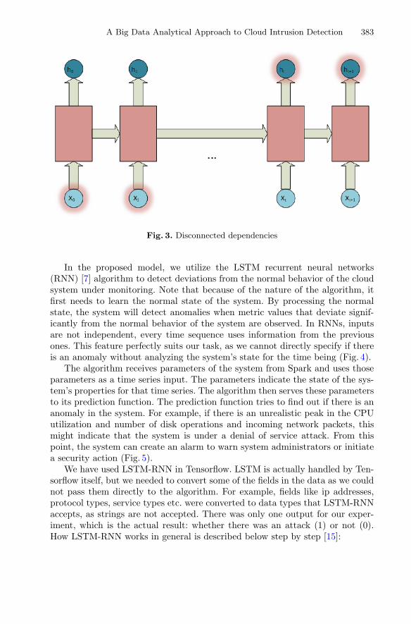
A Big Data Analytical Approach to Cloud Intrusion Detection 383
Fig. 3. Disconnected dependencies
In the proposed model, we utilize the LSTM recurrent neural networks(RNN) [7] algorithm to detect deviations from the normal behavior of the cloudsystem under monitoring. Note that because of the nature of the algorithm, itfirst needs to learn the normal state of the system. By processing the normalstate, the system will detect anomalies when metric values that deviate signif-icantly from the normal behavior of the system are observed. In RNNs, inputsare not independent, every time sequence uses information from the previousones. This feature perfectly suits our task, as we cannot directly specify if thereis an anomaly without analyzing the system’s state for the time being (Fig. 4).
The algorithm receives parameters of the system from Spark and uses thoseparameters as a time series input. The parameters indicate the state of the sys-tem’s properties for that time series. The algorithm then serves these parametersto its prediction function. The prediction function tries to find out if there is ananomaly in the system. For example, if there is an unrealistic peak in the CPUutilization and number of disk operations and incoming network packets, thismight indicate that the system is under a denial of service attack. From thispoint, the system can create an alarm to warn system administrators or initiatea security action (Fig. 5).
We have used LSTM-RNN in Tensorflow. LSTM is actually handled by Ten-sorflow itself, but we needed to convert some of the fields in the data as we couldnot pass them directly to the algorithm. For example, fields like ip addresses,protocol types, service types etc. were converted to data types that LSTM-RNNaccepts, as strings are not accepted. There was only one output for our exper-iment, which is the actual result: whether there was an attack (1) or not (0).How LSTM-RNN works in general is described below step by step [15]:
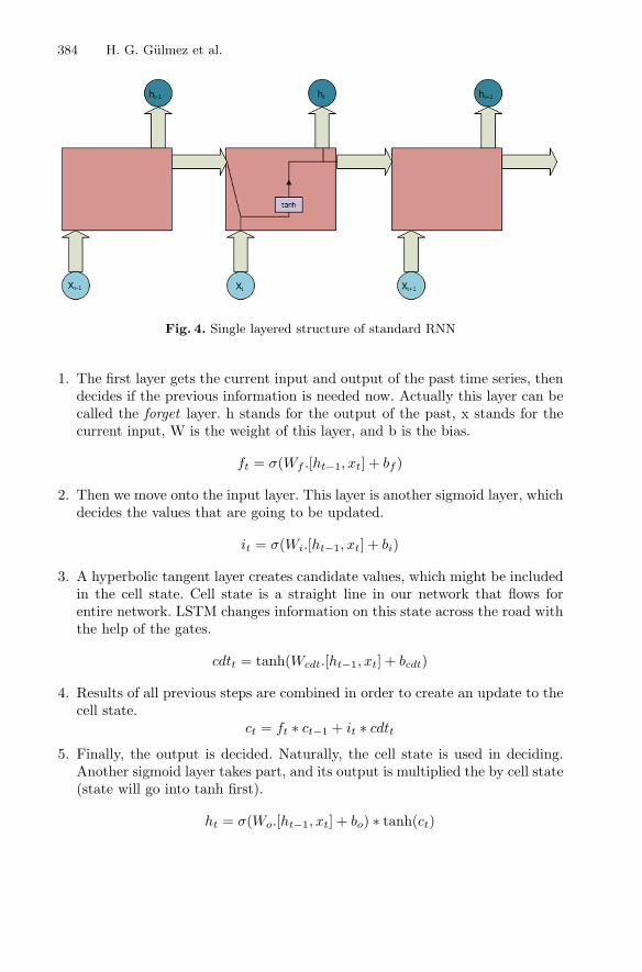
384 H. G. Gulmez et al.
Fig. 4. Single layered structure of standard RNN
1. The first layer gets the current input and output of the past time series, thendecides if the previous information is needed now. Actually this layer can becalled the forget layer. h stands for the output of the past, x stands for thecurrent input, W is the weight of this layer, and b is the bias.
ft = σ(Wf .[ht−1, xt] + bf )
2. Then we move onto the input layer. This layer is another sigmoid layer, whichdecides the values that are going to be updated.
it = σ(Wi.[ht−1, xt] + bi)
3. A hyperbolic tangent layer creates candidate values, which might be includedin the cell state. Cell state is a straight line in our network that flows forentire network. LSTM changes information on this state across the road withthe help of the gates.
cdtt = tanh(Wcdt.[ht−1, xt] + bcdt)
4. Results of all previous steps are combined in order to create an update to thecell state.
ct = ft ∗ ct−1 + it ∗ cdtt
5. Finally, the output is decided. Naturally, the cell state is used in deciding.Another sigmoid layer takes part, and its output is multiplied the by cell state(state will go into tanh first).
ht = σ(Wo.[ht−1, xt] + bo) ∗ tanh(ct)
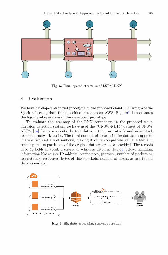
A Big Data Analytical Approach to Cloud Intrusion Detection 385
Fig. 5. Four layered structure of LSTM-RNN
4 Evaluation
We have developed an initial prototype of the proposed cloud IDS using ApacheSpark collecting data from machine instances on AWS. Figure 6 demonstratesthe high-level operation of the developed prototype.
To evaluate the accuracy of the RNN component in the proposed cloudintrusion detection system, we have used the “UNSW-NB15” dataset of UNSWADFA [14] for experiments. In this dataset, there are attack and non-attackrecords of network traffic. The total number of records in the dataset is approx-imately two and a half millions, making it quite comprehensive. The test andtraining sets as partitions of the original dataset are also provided. The recordshave 49 fields in total, a subset of which is listed in Table 1 below, includinginformation like source IP address, source port, protocol, number of packets onrequests and responses, bytes of those packets, number of losses, attack type ifthere is one etc.
Fig. 6. Big data processing system operation

386 H. G. Gulmez et al.
We have simulated the data so that the system behaves like the data arestreaming. At first, a training set is provided for LSTM-RNN, which runs onTensorFlow [19], which is an open-source machine learning framework. With thehelp of the model that is created on the framework, the system decides whethera record seems like an attack or not. We ran the model using 50000 records fortraining, and 650000 records for testing. The error rate was below 7%, which isa promising accuracy for intrusion detection.
Table 1. UNSW-NB15 parameters
No. Name Type Description
1 srcip Nominal Source IP address
2 sport Integer Source port number
3 dstip Nominal Destination IP address
4 dsport Integer Destination port number
5 proto Nominal Transaction protocol
6 state Nominal Indicates to the state and its dependent protocol, e.g. ACC,CLO, CON, ECO, ECR, FIN, INT, MAS, PAR, REQ, RST,TST, TXD, URH, URN, and (-) (if not used state)
7 dur Float Record total duration
8 sbytes Integer Source to destination transaction bytes
9 dbytes Integer Destination to source transaction bytes
10 sttl Integer Source to destination time to live value
11 dttl Integer Destination to source time to live value
12 sloss Integer Source packets retransmitted or dropped
13 dloss Integer Destination packets retransmitted or dropped
14 service Nominal http, ftp, smtp, ssh, dns, ftp-data, irc and (-) if not much usedservice
15 Sload Float Source bits per second
16 Dload Float Destination bits per second
17 Spkts Integer Source to destination packet count
18 Dpkts Integer Destination to source packet count
19 swin Integer Source TCP window advertisement value
20 dwin Integer Destination TCP window advertisement value
21 stcpb Integer Source TCP base sequence number
22 dtcpb Integer Destination TCP base sequence number
. . . . . . . . . . . .
48 attack cat Nominal The name of each attack category. In this data set, ninecategories e.g. Fuzzers, Analysis, Backdoors, DoS Exploits,Generic, Reconnaissance, Shellcode and Worms
49 Label Binary 0 for normal and 1 for attack records

A Big Data Analytical Approach to Cloud Intrusion Detection 387
5 Conclusion
In this work, we proposed an intrusion detection system for cloud computingthat leverages big data analytics with recurrent neural networks. We have imple-mented an initial prototype of the proposed architecture with Apache Spark andevaluated the performance of recurrent neural networks on a network attackdataset, which provided promising attack detection accuracy results. We haveused LSTM-RNN algorithm in Tensorflow to detect attacks in the network.LSTM-RNN has been picked as we were interested with using time series data.Results of this work looked promising about integrating big data analytics tointrusion detection in cloud. Our future work will focus on the integration ofa deep reinforcement learning based model, which will provide automated self-healing of cloud systems by learning from the consequences of attacks on thesystem, thereby avoiding states that are vulnerable to attacks. We will alsoexperiment with real data streams gathered using cloud APIs and quantify thedelays of big data processing as well as the mean time to detect attacks andrecover in major cloud platforms. Extensive experimentation with various attacktypes on cloud systems will be conducted to evaluate and optimize the big dataanalytics-based intrusion detection framework.
Acknowledgement. This work was supported by Middle East Technical Universityunder grant number: YOP-312-2018-2819.
References
1. Apache: Apache kafka, a distributed streaming platform. https://kafka.apache.org/. Accessed Apr 2018
2. Apache: Apache spark, lightning-fast unified analytics engine. https://spark.apache.org/. Accessed Apr 2018
3. AWS: Amazon kinesis. https://aws.amazon.com/kinesis/. Accessed Apr 20184. Bharadwaja, S., Sun, W., Niamat, M., Shen, F.: Collabra: a xen hypervisor based
collaborative intrusion detection system. In: 2011 Eighth International Conferenceon Information Technology: New Generations, pp. 695–700, April 2011. https://doi.org/10.1109/ITNG.2011.123
5. Casas, P., Soro, F., Vanerio, J., Settanni, G., D’Alconzo, A.: Network security andanomaly detection with big-DAMA, a big data analytics framework. In: 2017 IEEE6th International Conference on Cloud Networking (CloudNet), pp. 1–7, September2017. https://doi.org/10.1109/CloudNet.2017.8071525
6. DL4J: A beginner’s guide to recurrent networks and LSTMs. https://deeplearning4j.org/lstm.html. Accessed Apr 2018
7. Hochreiter, S., Schmidhuber, J.: Long short-term memory. Neural Comput. 9(8),1735–1780 (1997)
8. Kim, J., Kim, H.: Applying recurrent neural network to intrusion detection withHessian free optimization. In: Kim, H., Choi, D. (eds.) WISA 2015. LNCS, vol.9503, pp. 357–369. Springer, Cham (2016). https://doi.org/10.1007/978-3-319-31875-2 30
388 H. G. Gulmez et al.
9. Kumar, R.S.S., Wicker, A., Swann, M.: Practical machine learning for cloud intru-sion detection: challenges and the way forward. In: Proceedings of the 10th ACMWorkshop on Artificial Intelligence and Security, AISec 2017, pp. 81–90. ACM,New York (2017). https://doi.org/10.1145/3128572.3140445
10. Li, Z., Sun, W., Wang, L.: A neural network based distributed intrusion detectionsystem on cloud platform. In: 2012 IEEE 2nd International Conference on CloudComputing and Intelligence Systems, vol. 01, pp. 75–79, October 2012. https://doi.org/10.1109/CCIS.2012.6664371
11. Lipton, Z., Elkan, C., Berkowitz, J.: A critical review of recurrent neural networksfor sequence learning. Accessed Apr 2015
12. Maiero, C., Miculan, M.: Unobservable intrusion detection based on call traces inparavirtualized systems. In: Proceedings of the International Conference on Secu-rity and Cryptography, pp. 300–306, July 2011
13. Mishra, P., Pilli, E.S., Varadharajan, V., Tupakula, U.: Intrusion detection tech-niques in cloud environment: a survey. J. Netw. Comput. Appl. 77, 18–47 (2017).https://doi.org/10.1016/j.jnca.2016.10.015. http://www.sciencedirect.com/science/article/pii/S1084804516302417
14. Moustafa, N., Slay, J.: UNSW-NB15: a comprehensive data set for network intru-sion detection systems (UNSW-NB15 network data set). In: Proceedings of theMilitary Communications and Information Systems Conference, pp. 1–6 (2015)
15. Olah, C.: Understanding LSTM networks. http://colah.github.io/posts/2015-08-Understanding-LSTMs/. Accessed Apr 2018
16. Pandeeswari, N., Kumar, G.: Anomaly detection system in cloud environment usingfuzzy clustering based ANN. Mob. Netw. Appl. 21(3), 494–505 (2016). https://doi.org/10.1007/s11036-015-0644-x
17. Sharif, M.I., Lee, W., Cui, W., Lanzi, A.: Secure in-VM monitoring using hardwarevirtualization. In: Proceedings of the 16th ACM Conference on Computer andCommunications Security, CCS 2009, pp. 477–487. ACM, New York (2009). http://doi.acm.org/10.1145/1653662.1653720
18. Sinanc, D., Demirezen, U., Sagiroglu, S.: Evaluations of big data processing. Serv.Trans. Big Data 3, 44–54 (2016). https://doi.org/10.29268/stbd.2016.3.1.4
19. TensorFlow: an open source machine learning framework for everyone. https://www.tensorflow.org/. Accessed Apr 2018
20. Yin, C., Zhu, Y., Fei, J., He, X.: A deep learning approach for intrusion detectionusing recurrent neural networks. IEEE Access 5, 21954–21961 (2017). https://doi.org/10.1109/ACCESS.2017.2762418

Short Track

Context Sensitive Efficient Automatic ResourceScheduling for Cloud Applications
Lun Meng1 and Yao Sun2(&)
1 College of Public Administration, Hohai University, Nanjing 210098, China2 School of Software Engineering, Jinling Institute of Technology,
Nanjing 211169, [email protected]
Abstract. Nowadays applications in cloud computing often use containers astheir service infrastructures to provide online services. Applications deployed inlightweight containers can be quickly started and stopped, which adapt tochanging resource requirements brought from workload fluctuation. Existingworks to schedule physical resources often model applications’ performanceaccording to a training dataset, but they cannot self-adapt dynamic deploymentenvironment. To address this above issue, this paper proposes a feedback basedphysical resource scheduling approach for containers to deal with the significantchanges of physical resources brought from dynamic workloads. First, we modelapplications’ performance with a queue-based model, which represents thecorrelations between workloads and performance metrics. Second, we predictapplications’ response time by adjusting the parameters of the application per-formance model with a fuzzy Kalman filter. Finally, we schedule physicalresources according to the predicted response time. Experimental results showthat our approach can adapt to dynamic workloads and achieve highperformance.
Keywords: Resource scheduling � Cloud application � Fuzzy logicKalman filter
1 Introduction
Nowadays, applications in cloud computing are often composed with fine-grainedisolated service components that use lightweight communication protocols to cooperatewith each other. These autonomous components update independently, which meetsthe changing requirements of cloud applications. Furthermore, different components ofan application have various resource requirements, so dynamic resource scheduling forcomponents is important for cloud applications, especially in the real scenario withsignificant fluctuate workloads. Cloud applications often use containers (e.g., Docker)as their service infrastructures to provide online cloud-based services. A container is alightweight stand-alone executable software package that includes everything neededto run it, which isolates applications from its surroundings and avoids conflicts betweenteams running different applications on the same infrastructure. An applicationdeployed in a container always runs the same regardless of environment. Lightweight
© Springer International Publishing AG, part of Springer Nature 2018M. Luo and L.-J. Zhang (Eds.): CLOUD 2018, LNCS 10967, pp. 391–397, 2018.https://doi.org/10.1007/978-3-319-94295-7_27

containers can be quickly started and stopped, so it can adapt to changing resourcerequirements brought from workload fluctuation in cloud computing. Existing worksoften model an application’s performance, and then schedule resources with physicalhosts or virtual machines. However, modeling an application’s performance oftenrequires the domain knowledge of the application. Moreover, since they set theparameters of the application’s performance model according to a training dataset,these approaches cannot self-adapt to dynamic deployment environment. The contri-butions of this paper are listed as follows:
• We model applications’ performance with a Jackson network model, which auto-matically presents the correlations between workloads and performance metricswithout domain knowledge and human intervention.
• We predict workloads with a fuzzy Kalman filter, which can conveniently adapt todynamic deployment environments by adjusting the parameters of applications’performance model.
• We have implemented a prototype system and conducted extensive experiments inreal scenarios to validate the proposed approach in predicting workloads andscheduling resources.
2 Resource Scheduling Approach
2.1 Queueing Based Performance Model
Response time is a key QoS (Quality of Service) metric of cloud applications, which isoften decided by dynamic workloads and allocated physical resources. We use a queue-based model based on a Jackson network to model applications’ performance, and themodel presents the correlations among workloads, resources and response time; use aKalman filter to predict workloads and response time; use a feedforward controllerbased on fuzzy logic to rectify the parameters of the filter to precisely predict theresponse time.
Processing requests includes that a user sends a request to an application, therequest is capsuled as an event, the event is processed by many components insequence, and then a response is sent back to the user. When one component has manyinstances, the application uses a round robin scheduling strategy to process the request.We model a cloud application composed of many components with a Jackson queueingnetwork, where f is a user’s request flow, j is an application component, i is the ithinstance of the jth component. Each request flow is processed by n componentsj1; j2; . . .; jn; each component j has m instances j(ik) ð1� k�mÞ; and each componentruns in a container. Various components have different resource requirements (e.g.,CPU and I/O intensive), and we define the resource preference (rpi) of component j asthe resource type with the highest resource utilization; uj ð0� uj � 1Þ is the resourceutilization of rpj, and u0j is the resource utilization of rpj with no workload; rji is theconcurrency number (i.e., the number of requests in a second) of instance i of com-ponent j, which fits for the Poisson distribution; Tji is the processing time of instancei of component j, and Tj is the average processing time of component j; d is the
392 L. Meng and Y. Sun

transmitting time of a request flow f; B is the response time of a request flow f; sj is thecorrelation coefficient between workloads and resource utilization. Then, we get aJackson network flow, and the performance formula is described as follows:
uj ¼X
iðu0j þ sj � cji � TjiÞ;
B ¼ dþX
j
Tj1� uj=mj
;
where we can get uj, u0j, rji and B by monitoring applications; get sj from experiencewith historical data; predict Tji and d. We aim at provisioning resources to guaranteeB in a predefined range.
2.2 Kalman Filter Based Response Time Prediction
The Kalman filter is an optimal linear state estimation approach, which recursivelypredicts the next value using the previous predicted value and the current monitoringdata instance [1]. The Kalman filter formula are as follows:
Xðkþ 1Þ ¼ FðkÞXðkÞþQðkÞ;
ZðkÞ ¼ HðkÞXðkÞþRðkÞ;
where X(kÞ ¼ ðTj; dÞT8j is a prediction matrix representing the processing times ofcomponents; Z(k) is the observed matrix of X(k); HðkÞ ¼ ðuj; u0j; cji;BÞT8i representsthe workloads, resource utilization and response time; Q(k) is a process excitation noisecovariance matrix, which fits for QðkÞ�Nð0;QÞ; R(k) is a measurement noisecovariance matrix, which fits for RðkÞ�Nð0;RÞ. Q(k) and R(k) are generally set as zeromean white noise [2]. However, uncertain workloads change over time, so Q(k) and R(k) should adapt to dynamic workloads as follows:
Qk ¼ TQ;
Rk ¼ UR;
where T and U are time-varying adjustment parameters, and then we can get theprediction formula as follows:
Xðkþ 1jkÞ ¼ Fðkþ 1jkÞXðkjkÞ;
Zðkþ 1jkþ 1Þ ¼ HðkÞXðkþ 1jkÞ;
where Xðkþ 1jkÞ is the predicted time of processing requests, and ZðkÞ is the predictedvalue of the status, and then we can predict the response time as follows:
Context Sensitive Efficient Automatic Resource Scheduling for Cloud Applications 393
Xðkþ 1jkþ 1Þ ¼ Xðkþ 1jkÞþKðkþ 1Þ � ðZðkþ 1jkþ 1Þ � Zðkþ 1jkþ 1ÞÞ;Kðkþ 1Þ ¼ Pðkþ 1jkÞHðkÞTðHðkÞPðkþ 1jkÞÞHðkÞT þ Tðkþ 1ÞRÞ�1;
Pðkþ 1jkþ 1Þ ¼ ðIn � Kðkþ 1ÞHðkÞÞPðkþ 1jkÞ;Pðkþ 1jkÞ ¼ Fðkþ 1ÞPðkjkÞFðkþ 1jkÞT þUðkþ 1ÞQ:
The Kalman filter rectifies the predicted value with the last calculated value in eachiteration, so it does not require historical data instances. However, the typical Kalmanfilter cannot process the irregular time-varying data instances, so it requires feedback-based methods to online adjust noises and excitation matrixes. The residual errorr ¼ ZðkÞ � ZðkÞ represents that the deviation between the predicted value and themonitored one, and then we ought to modify the constructed model, if the deviationviolates the predefined threshold.
2.3 Resource Scheduling
We online schedule physical resources based on the predicted response time. Weinitiate the Kalman filter by defining parameters as follows: the noise parameters T andU of the Kalman filter, the maximum and minimum of resource utilization, and themaximum response time of a service instance (Input); a fuzzy logic function adaptivelyadjusts the parameters of the EKF model; a response time function using EKF’s outputscalculates response time; a migration function migrates containers; a expansion func-tion expands containers; a contraction function contracts containers. Then, we predictresponse time as follows: model an application with a Jackson network queue; onlinepredict response time with a Kalman filter; adjust the Kalman filter with a fuzzyfunction; estimate the response time based on the prediction model. Finally, wemigrate, expand and contract a container as follows:
• Migrate containers: the resource utilization of a container does not reach the upperlimit, but the resource utilization of the located physical host reaches to the upperlimit. Then, the scheduler migrates the container to the host with sufficient physicalresources. The scheduler persists a source container as an image reserving theapplication’s state, destroys the source container, and then is initiates a targetcontainer from the image in the target host.
• Expand containers: the resource utilization of a container reaches the upper limit,and the schedule initiates new containers in selected physical hosts.
• Contract containers: the resource utilization of many instances of an application islower than expected value, and then we reduce the number of instances.
3 Experiment
We set up a cluster composed of six hosts. Each host has an Intel Core i7 CPU3.4 GHz, an 8 G memory and a gigabit ethernet network interface, and runs CenOS 7and Docker 1.7. We have a Master node, four Slave nodes (i.e., Slave 1–4), and a
394 L. Meng and Y. Sun

workload generator node running JMeter. We deploy a typical cloud application WebServing in Cloudsuite (http://cloudsuite.ch//pages/benchmarks/webserving/) that is abenchmark suite for cloud services.
JMeter simulates workloads in a cyclical change model, a stable model, a steadyrise model and a sudden decline model. Admission control is a widely used approach ofscheduling resources. Since the admission controller takes a long period to converge,the fixed parameters cannot adapt to changing irregular workloads [3]. In the experi-ment, we compare our approach with the admission control approach. In initialization,we deploy six services on Slave 1 and the rest six services on Slave 2. As shown inFig. 1, the experimental results are described as follows:
In the period of the 0–200th second, we simulate stable workloads with 300 visitsper second to initialize the Kalman filter. In the period of the 200–300th second, wesimulate dynamic workloads with 30–60 visits per second, and the response timeincreases. Since the resource utilization of services does not reach the upper limit,expansion does not occur. As the resource utilization of Slave 1 reaches the upper limit,three services on Slave 1 are migrated to Slave 3 and Slave 4, and the response timefluctuates in a narrow range. In the period of the 300–400th second, we simulate stableworkloads with 50 visits per second, and the response time also stable. In the period ofthe 600–700th second, we simulate sudden rise workloads with 50–100 visits persecond in the 650th second, some services on Slave 1 and Slave 2 are expanded, and theresponse time stably decreases. In the period of the 700–800th second, we simulatesudden decline workloads with 100–30 visits per second in the 750th second, and someservices are contracted.
The experimental results show that the response time keeps stable in 30–40 microseconds, which demonstrates that our approach can adapt to dynamic workloads.
20
30
40
50
60
70
80
90
1 0 0 2 0 0 3 0 0 4 0 0 5 0 0 6 0 0 7 0 0 8 0 0 9 0 0 1 0 0 0 1 1 0 0 1 2 0 0 1 3 0 0 1 4 0 0 1 5 0 0 1 6 0 0
RES
PON
SE T
IME
MS
TIME S
Our Approach
Admission Control
Fig. 1. Responses time
Context Sensitive Efficient Automatic Resource Scheduling for Cloud Applications 395

4 Related Works
Existing works of provisioning resources often use machine learning, fuzzy logic andadmission control to train models and calculate parameters. Lama and Zhou [4] predictthe spike of applications’ resource requirements, and provision physical resources inthe quality of service (QoS) constraints. Cao et al. [5] estimate the supported workloadsaccording to the allocated resources, and use an admission control method to guaranteeQoS by denying overloading requests. Cherkasova and Phaal [6] model the correlationsbetween workloads and throughput, estimate resource requirements, and acceptrequests with admission mechanism. Robertsson et al. [7] use a linearity model topredict resource utilization for guaranteeing QoS. Xu et al. [8] consider the perfor-mance overhead of VM and trace the changes of applications’ resources in virtual-ization environment. These approaches train models and get parameters with a statictraining dataset, so cannot adapt to dynamic fluctuate workloads.
5 Conclusion
This paper proposes a feedback based physical resource scheduling approach forcontainers to deal with the significant changes of physical resources brought fromdynamic workloads. First, we model applications’ performance with a Jackson networkmodel, which presents the correlations between workloads and performance metrics.Second, we predict applications’ response time by adjusting the parameters of appli-cations’ performance model with a fuzzy Kalman filter. Finally, we schedule physicalresources based on the predicted response time. Experimental results show that themaximum error of our approach in predicting response time is only about 10%.
Acknowledgment. This work was supported by the National Social Science Foundation ofChina (grant number 16CXW027), fundamental research funds for the central universities (grant2014B00514) and the Ministry of Education of Humanities and Social Science project (grant15YJCZH117).
References
1. Kalman, R.E.: A new approach to linear filtering and prediction problems. Trans. ASME-J.Basic Eng. 82, 35–45 (1960)
2. Sinopoli, B., Schenato, L., Franceschetti, M., et al.: Kalman filtering with intermittentobservations. IEEE Trans. Autom. Control 49(9), 1453–1464 (2004)
3. Lu, C., Lu, Y., Abdelzaher, T.F., et al.: Feedback control architecture and designmethodology for service delay guarantees in web servers. IEEE Trans. Parallel Distrib. Syst.17(9), 1014–1027 (2006)
4. Lama, P., Zhou, X.: Efficient server provisioning with control for end-to-end response timeguarantee on multitier clusters. IEEE Trans. Parallel Distrib. Syst. 23(1), 78–86 (2012)
5. Cao, J., Zhang, W., Tan, W.: Dynamic control of data streaming and processing in avirtualized environment. IEEE Trans. Autom. Sci. Eng. 9(2), 365–376 (2012)
396 L. Meng and Y. Sun

6. Cherkasova, L., Phaal, P.: Session-based admission control: a mechanism for peak loadmanagement of commercial web sites. IEEE Trans. Comput. 51(6), 669–685 (2002)
7. Robertsson, A., Wittenmark, B., Kihl, M., et al.: Design and evaluation of load control in webserver systems. In: Proceedings of IEEE American Control Conference, vol. 3, pp. 1980–1985(2004)
8. Xu, C.Z., Rao, J., Bu, X.: URL: a unified reinforcement learning approach for autonomiccloud management. J. Parallel Distrib. Comput. 72(2), 95–105 (2012)
Context Sensitive Efficient Automatic Resource Scheduling for Cloud Applications 397

A Case Study on Benchmarking IoTCloud Services
Kevin Grunberg and Wolfram Schenck(B)
Faculty of Engineering and Mathematics, Center for Applied Data Science Gutersloh,Bielefeld University of Applied Sciences, Bielefeld, Germany
kevin [email protected], [email protected]
Abstract. The Internet of Things (IoT) is on the rise, forming net-works of sensors, machines, cars, household appliances, and other physi-cal items. In the industrial area, machines in assembly lines are connectedto the internet for quick date exchange and coordinated operation. Cloudservices are an obvious choice for data integration and processing in the(industrial) IoT. However, manufacturing machines have to exchangedata in close to real-time in many use cases, requiring small round-triptimes (RTT) in the communication between device and cloud. In thisstudy, two of the major IoT cloud services, Microsoft Azure IoT Huband Amazon Web Services IoT, are benchmarked in the area of NorthRhine-Westphalia (Germany) regarding RTT, varying factors like timeof day, day of week, location, inter-message interval, and additional dataprocessing in the cloud. The results show significant performance differ-ences between the cloud services and a considerable impact of some of theaforementioned factors. In conclusion, as soon as (soft) real-time condi-tions come into play, it is highly advisable to carry out benchmarking inadvance to identify an IoT cloud workflow which meets these conditions.
Keywords: Cloud benchmarking · Internet of Things · IoTIndustrial IoT · Cyberphysical systems · Round-trip timeMicrosoft Azure IoT Hub · Amazon Web Services IoT
1 Introduction
During the last decade, cloud computing has become a highly popular approachto provide scalable and flexible hardware and software infrastructure at variousservice levels (infrastructure as a service [IasS], platform as a service [PaaS],software as a service [SaaS]) [1]. With the Internet of Things (IoT) being on therise, a new use case for cloud computing emerges. In the IoT, physical objects likesensors, machines, cars, household appliances, and other items are connected viathe internet to enable interaction and cooperation of these objects. Applicationareas of the IoT are, among others, transportation, healthcare, smart homes andindustrial environments [2]. IoT devices typically generate and transmit dataat regular intervals. This data is integrated, processed, and monitored (e.g., via
c© Springer International Publishing AG, part of Springer Nature 2018M. Luo and L.-J. Zhang (Eds.): CLOUD 2018, LNCS 10967, pp. 398–406, 2018.https://doi.org/10.1007/978-3-319-94295-7_28

A Case Study on Benchmarking IoT Cloud Services 399
Data Genera on
Device Client (D2C) Eventhub Client (C2D)
Azure IoT Hub Endpoint:„messages/events“
Data Genera on
AWSMq Client (D2C) AWSMq Client (C2D)Publishing to Topic: Subscrip on to Topic:Benchmark Benchmark
DeviceGateway
AWS IoT
A B
Fig. 1. Message flow between benchmarking applications (gray box incl. data genera-tion) and cloud services. A: For MS Azure IoT Hub. B: For AWS IoT.
mobile devices or web applications), and commands for corrective actions (whichare either manually or automatically generated) are sent back to the devices [3].Furthermore, IoT devices may interact directly with each other.
It is an obvious approach to use the cloud for data integration and process-ing [4]. The major cloud service providers (CSP) have established meanwhilespecialized services for data collection from IoT devices, supporting popularprotocols like MQTT or AMQP. However, many application scenarios in theIoT—especially in the industrial area—rely on operations taking place in closeto real-time: For example, when manufacturing machines are controlled via appsrunning in the cloud, or when these machines use the cloud as central instancefor data exchange to coordinate their work in an assembly line. Therefore itis important that cloud platforms used for these purposes process and forwardmessages with small latency and consistent availability and performance.
Although many studies on cloud benchmarking in general exist, we are notaware of any study which addresses especially the performance of IoT cloud ser-vices. As a first step in this direction, we present benchmarking data collectedfrom Microsoft Azure IoT Hub (MAIH) and Amazon Web Services IoT (AWSI)at three different locations in North Rhine-Westphalia (NRW; Germany) aroundSept./Oct. 2017. This data collection was part of a larger research project for alocal mechanical engineering company to integrate their products in the indus-trial IoT. Despite this local scope, we are convinced that some general conclusionscan be drawn from our data.
2 Previous Work
Studies on cloud benchmarking address mostly the PaaS and IaaS levels. Con-cerning PaaS, Binnig et al. [5] point out that classic benchmarking approachesare not well suited for cloud APIs because resources are usually scaled up auto-matically with increasing load. They suggest to concentrate on scalability, cost,coping with peak load, and fault tolerance. Agarwal and Prasad [6] carried outa comprehensive benchmarking study on the storage services of the MicrosoftAzure cloud platform, especially for high-performance computing. In their view,benchmarking is definitely required to understand the performance capabilities

400 K. Grunberg and W. Schenck
7am 8am 9am 10am 11am 12pm 1pm 2pm 3pm 4pmTime of Day
20
40
60
80
100
120
140
160
180
200
220R
ou
nd
Tri
pT
ime
in m
s Microsoft Azure IoT Hub / Industrial Estate
Microsoft Azure IoT Hub / Residential Area
Microsoft Azure IoT Hub / University Campus
Amazon Web Services IoT / Industrial Estate
Amazon Web Services IoT / Residential Area
Amazon Web Services IoT / University Campus
Fig. 2. RTT measurements, varying time of day and location. Each data point depictsthe median value and interquartile range of around 100 measurements.
of the underlying cloud platforms because the cloud service offerings are usuallyonly best-effort based without any performance guarantees. In a similar spirit,Kossmann et al. [7] compared the performance of major CSPs in transactionprocessing. Their results show that the services vary dramatically when it comesto end-to-end performance, scalability, and cost—although the price matrices ofthe CSPs are very similar in terms of network bandwidth, storage cost, and CPUcost (see also [8] for a holistic evaluation approach). The study by Bermbach andWittern [9] is related to our work because the authors use response latency asperformance measure for web API quality. They observed 15 different web APIsover a longer time period from different locations in the world. They results showthat web API quality is very volatile over time and location, and that develop-ers have to take this into account from an architectural and engineering pointof view.
High variability is also observed at the IaaS level. Gillam et al. [10] and Zantand Gagnaire [11] carried out a large set of benchmarks on virtual machines(VM) of different specifications and from different CSPs. Even if the virtualresources are of the same specification, the observed variability is substantial(e.g., regarding CPU and memory performance). To help customers to choose thebest cloud platform for their needs, benchmarking results could be made avail-able in publicly available databases (as in [10]), or tools for easier benchmarkingcould be developed. Following the second approach, Cunha et al. [12] imple-mented “Cloud Crawler” for describing and automatically executing applicationperformance tests in IaaS clouds for different virtual machine configurations.
3 Methods
Performance Measure. The quality of data transfer to and from cloud servicescan vary along two main dimensions: throughput (number and/or size of mes-sages per time unit) and latency. Using throughput as performance measure,

A Case Study on Benchmarking IoT Cloud Services 401
Table 1. Mean values and standard deviations (in brackets) of the RTT median val-ues (varying over time of day) shown in Fig. 2 to illustrate the systematic differencesbetween locations. Values given in ms.
Location
Industrial estate Residential area University campus
MS Azure IoT Hub 47.7 (2.0) 62.8 (1.4) 47.2 (2.7)
AWS IoT 191.8 (2.5) 199.1 (1.4) 185.4 (2.8)
however, is problematic because many cloud services automatically scale up theavailable communication resources with increasing load [13]. For this reason,and because we aim on real-time performance in the context of our study, whichrequires message transfers with low latency, we use the round-trip time (RTT) inour benchmarking. RTT is defined here as the time difference between sending amessage to a communication endpoint (time of sending) and receiving the samemessage back from this endpoint (time of arrival).
Microsoft Azure IoT Hub (MAIH). The benchmarking application for MAIHwas implemented using the .NET SDK provided by Microsoft [14]. On the clientside, a so-called “DeviceClient” has to be created and initialized for sendingmessages to the IoT Hub (see Fig. 1A). Within the Azure cloud, messages areforwarded to an “EventHub” endpoint. Within the client, a subscription to thisendpoint is created so that messages are automatically received back. (MAIHserver location: Western Europe)
Amazon Web Services IoT (AWSI). The benchmarking application for AWSIhas a similar structure but is based on the JAVA SDK provided by Amazon[15]. An important step is to register the device at the AWSI device gateway(see Fig. 1B) as a “thing” with a unique identifier (“topic”) under which it ispublished. The same topic is used for the subscription to receive the messagesback from the device gateway. (AWSI server loc.: Frankfurt/Main, Germany)
Messages. The content of the sent messages was a single boolean value1 whichwas embedded into a JSON container (size: 250 Bytes). This container also con-tained the time of sending as timestamp. In most benchmarking tests, messageswere sent every two seconds. To measure a single data point, about 100 messageswere sent; the median and the interquartile range of this sample are shown inmost of the figures in the results section. The benchmarking applications wererun on a notebook with a quadcore CPU (Intel i7-4712MQ). Messages retrievedunder a CPU load of more than 20% were discarded to eliminate CPU load asa cause of variability [13]. The percentage of discarded messages was in the lowsingle-digit range. Messages were transferred via MQTT.
1 Pretests did not show any significant RTT differences between different basic datatypes like int, float, etc.

402 K. Grunberg and W. Schenck
Wed. 27.09 Thu. 28.09 Fri. 29.09 Sat. 30.09 Sun. 01.10 Mon. 02.10 Tue. 03.10Day of week
0
50
100
150
200
Ro
un
dT
rip
Tim
e in
ms
Microsoft Azure IoT Hub Amazon Web Services IoT
Fig. 3. RTT measurements, varying day of week. Each data point depicts the medianvalue and interquartile range of around 100 measurements.
Locations. Benchmarking took place at three different locations in NRW (Ger-many): (1) At a mechanical engineering company within an industrial park inRheda-Wiedenbruck (denoted as “industrial estate” in the following; connectionto internet via optic fiber); (2) at a residential building in Herzebrock-Clarholz(“residential area”; connection to internet via DSL over regular copper phonelines); (3) at the main campus of Bielefeld University of Applied Sciences inBielefeld (“university campus”; connection to internet via the German NationalResearch and Education Network [DFN] [optic fiber]).
4 Results
Time of Day and Location. In the first set of benchmarks, time of day andlocation were varied systematically. Figure 2 shows considerable RTT differencesbetween MAIH (mean median value: 52.5 ms) and AWSI (mean median value:192.1 ms) while performance stays nearly constant during the day. Interquartileranges vary during the day, and sometimes strong outliers with large RTT valueswere observed (not shown). Location has systematic impact too, with “universitycampus” exhibiting the smallest RTT values for both CSPs, followed by “indus-trial estate” and “residential area” (in this order; see Table 1). Measurementswere carried out around midweek.
Day of Week. RTT measurements were repeated between Sept. 27th andOct. 3rd at the residential area to check the impact of the day of the week.The results in Fig. 3 show small variability between the days of the week regard-ing median values with one notable exception: MAIH on Sunday with an RTTincrease of about 30%. Because this effect does not appear in the AWSI mea-surements carried out at nearly the same time, it can be most likely attributedto the Azure platform or to the connecting network route.
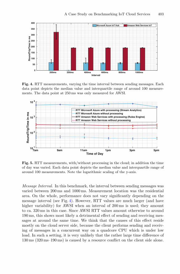
A Case Study on Benchmarking IoT Cloud Services 403
200ms 250ms 400ms 600ms 800ms 1000msInterval
0
50
100
150
200
250
300
350
400
Ro
un
dT
rip
Tim
e in
ms
Microsoft Azure IoT Hub Amazon Web Services IoT
Fig. 4. RTT measurements, varying the time interval between sending messages. Eachdata point depicts the median value and interquartile range of around 100 measure-ments. The data point at 250 ms was only measured for AWSI.
7am 9am 11am 1pm 3pm 5pmTime of Day
10 1
10 2
10 3
10 4
Ro
un
dT
rip
Tim
e in
ms
RTT Microsoft Azure with processing (Stream Analytics)RTT Microsoft Azure without processingRTT Amazon Web Services with processing (Rules Engine)RTT Amazon Web Services without processing
Fig. 5. RTT measurements, with/without processing in the cloud; in addition the timeof day was varied. Each data point depicts the median value and interquartile range ofaround 100 measurements. Note the logarithmic scaling of the y-axis.
Message Interval. In this benchmark, the interval between sending messages wasvaried between 200 ms and 1000 ms. Measurement location was the residentialarea. On the whole, performance does not vary significantly depending on themessage interval (see Fig. 4). However, RTT values are much larger (and havehigher variability) for AWSI when an interval of 200 ms is used; they amountto ca. 320 ms in this case. Since AWSI RTT values amount otherwise to around190 ms, this shows most likely a detrimental effect of sending and receiving mes-sages at around the same time. We think that the causes of this effect residemostly on the cloud server side, because the client performs sending and receiv-ing of messages in a concurrent way on a quadcore CPU which is under lowload. In such a setting, it is very unlikely that the rather large time difference of130 ms (320 ms–190 ms) is caused by a resource conflict on the client side alone.

404 K. Grunberg and W. Schenck
Additional Processing in the Cloud. For the (industrial) IoT, it is a common sce-nario that device data is processed in the cloud before it is sent back to anotherendpoint (e.g., data preprocessing in the cloud before data visualization on amobile device). As a benchmark for this use case, we sent in each message asingle float value to the cloud where it was multiplied by two and sent back. Forthis purpose, the workflows in the cloud had to be modified: Within MicrosoftAzure, messages are forwarded from the IoT Hub to the service “Stream Ana-lytics” where processing takes place. Afterwards, the “Service Bus” sends themodified messages back to a so-called “Queue Client” implemented as part of thebenchmarking application. In the AWS cloud, received messages are forwardedfrom the Device Gateway to the “Rules Engine” for processing. The processedmessages are made available under a new topic to which the MQTT client in thebenchmarking application is subscribed.
Benchmarks were carried out at the industrial estate. The results are shownin Fig. 5. Performance does not vary significantly during the course of the day,but the additional processing in the cloud has a clear impact on the RTT values.For AWSI, the mean value of the median values increases from 192.8 ms (withoutprocessing) to 304.3 ms (with processing). For MAIH, an increase from 49.2 ms(without processing) to 6336 ms (with processing) was observed. The latter is areally significant slowdown by a factor of 129.
5 Discussion and Outlook
Results of cloud benchmarking usually have to be taken with a grain of saltbecause there exist many uncontrollable factors along the route between clientand cloud servers [13]. Furthermore, CSPs may upgrade and modify their systemswithout notice. Therefore, we are well aware that our results only represent alocal snap-shot, and that similar performance measurements may be different inother parts of the world and in the future. For this reason, it is definitely notour goal to attribute good or bad performance to MAIH or AWSI in general.
However, our results clearly show that one has to be careful in choosingthe right cloud platform for IoT operations in one’s local area, especially if weconsider the use case of cyber-manufacturing systems (industrial IoT) which areintended to interact in real-time—not in the very strict sense of hard real-timeconditions, but in the sense of seamless coordination between machines (andmaybe machines and humans). Our data shows a clear performance advantagefor one of the two benchmarked CSPs, and how this pattern completely reversesin an extreme fashion as soon as additional processing of the data in the cloudis required. Mean performance and variability is rather stable when varying theday of week, the time of day, or the location. However, the latter factor hasa clearly visible and systematic impact on the performance of both CSPs. Aconsiderable performance drop could be observed for AWSI when decreasing thesending interval between messages to the usual RTT. This is a clear warningthat performance is subject to factors in an unexpected way (one message every200 ms does not look like heavy load, does it?).

A Case Study on Benchmarking IoT Cloud Services 405
Although the number of clients in a manufacturing line, which are indepen-dently connected to an IoT cloud service, is usually not that large comparedto e.g. the millions of smart home devices, it is definitely an important stepfor further benchmarking to increase the number of clients which send data inparallel to the cloud. Furthermore, we plan to repeat our measurements over alonger time period and, in addition, to vary message size. Message size is impor-tant because it is common that programmable logic controllers in manufacturingcollect sets of sensory and control variables and transmit them at once, e.g. toa local OPC-UA client which in turn forwards the data in the form of largerpackages to the cloud.
Given our already existing benchmarking results, we are convinced that man-ufacturing companies, when they move forward to cyberphysical production sys-tems, have to carefully plan the data flow to the cloud and to carry out corre-sponding benchmarks because it may depend strongly on the CSP if specificreal-time conditions for IoT data processing are met in the end.
Acknowledgements. We appreciate the general support by Dominik Osthues(Rheda-Wiedenbruck) for our benchmarking work. Furthermore, we thank MartinKohlhase (Bielefeld Univ. of Applied Sciences) for many helpful discussions.
References
1. Vaquero, L.M., Rodero-Merino, L., Caceres, J., Lindner, M.: A break in the clouds:towards a cloud definition. SIGCOMM Comput. Commun. Rev. 39(1), 50–55(2008)
2. Jeschke, S., Brecher, C., Meisen, T., Ozdemir, D., Eschert, T.: Industrial internetof things and cyber manufacturing systems. In: Jeschke, S., Brecher, C., Song,H., Rawat, D.B. (eds.) Industrial Internet of Things – Cybermanufacturing Sys-tems. SSWT, pp. 3–19. Springer, Cham (2017). https://doi.org/10.1007/978-3-319-42559-7 1
3. Lee, G.M., Crespi, N., Choi, J.K., Boussard, M.: Internet of things. In: Bertin,E., Crespi, N., Magedanz, T. (eds.) Evolution of Telecommunication Services: TheConvergence of Telecom and Internet: Technologies and Ecosystems. LNCS, vol.7768, pp. 257–282. Springer, Heidelberg (2013). https://doi.org/10.1007/978-3-642-41569-2 13
4. Gubbi, J., Buyya, R., Marusic, S., Palaniswami, M.: Internet of Things (IoT): avision, architectural elements, and future directions. Future Gener. Comput. Syst.29(7), 1645–1660 (2013)
5. Binnig, C., Kossmann, D., Kraska, T., Loesing, S.: How is the weather tomor-row?: towards a benchmark for the cloud. In: Proceedings of the 2nd InternationalWorkshop on Testing Database Systems, DBTest 2009, pp. 9:1–9:6. ACM, NewYork (2009)
6. Agarwal, D., Prasad, S.K.: AzureBench: benchmarking the storage services of theAzure cloud platform. In: 2012 IEEE 26th International Parallel and DistributedProcessing Symposium Workshops PhD Forum, pp. 1048–1057 (2012)

406 K. Grunberg and W. Schenck
7. Kossmann, D., Kraska, T., Loesing, S.: An evaluation of alternative architecturesfor transaction processing in the cloud. In: Proceedings of the 2010 ACM SIGMODInternational Conference on Management of Data, SIGMOD 2010, pp. 579–590.ACM, New York (2010)
8. Li, Z., O’Brien, L., Zhang, H.: Boosting metrics: measuring cloud services from theholistic perspective. Int. J. Cloud Comput. (IJCC) 2(4), 12–22 (2014)
9. Bermbach, D., Wittern, E.: Benchmarking web API quality. In: Bozzon, A., Cudre-Maroux, P., Pautasso, C. (eds.) ICWE 2016. LNCS, vol. 9671, pp. 188–206.Springer, Cham (2016). https://doi.org/10.1007/978-3-319-38791-8 11
10. Gillam, L., Li, B., O’Loughlin, J., Tomar, A.P.S.: Fair benchmarking for cloudcomputing systems. J. Cloud Comput.: Adv. Syst. Appl. 2(1), 6 (2013)
11. Zant, B.E., Gagnaire, M.: Performance and price analysis for cloud serviceproviders. In: 2015 Science and Information Conference (SAI), pp. 816–822 (2015)
12. Cunha, M., Mendonca, N., Sampaio, A.: A declarative environment for automaticperformance evaluation in IaaS clouds. In: 2013 IEEE Sixth International Confer-ence on Cloud Computing, pp. 285–292 (2013)
13. Bermbach, D., Wittern, E., Tai, S.: Cloud Service Benchmarking – Measuring Qual-ity of Cloud Services from a Client Perspective. Springer, Cham (2017). https://doi.org/10.1007/978-3-319-55483-9
14. Microsoft Corporation: Get started with Azure IoT Hub (.NET) – Microsoft Docs(2017). https://docs.microsoft.com/en-us/azure/iot-hub/iot-hub-csharp-csharp-getstarted. Accessed 08 Aug 2017
15. AWS Inc.: AWS IoT – Developer Guide (2017). http://docs.aws.amazon.com/iot/latest/developerguide/iot-dg.pdf. Accessed 02 Sept 2017

A Comprehensive Solution forResearch-Oriented Cloud Computing
Mevlut A. Demir(B), Weslyn Wagner, Divyaansh Dandona,and John J. Prevost
The University of Texas at San Antonio,One UTSA Circle, San Antonio, TX 78249, USA
{mevlut.demir,jeff.prevost}@utsa.edu, {weslyn.wagner,ubm700}@my.utsa.edu
Abstract. Cutting edge research today requires researchers to performcomputationally intensive calculations and/or create models and simu-lations using large sums of data in order to reach research-backed con-clusions. As datasets, models, and calculations increase in size and scopethey present a computational and analytical challenge to the researcher.Advances in cloud computing and the emergence of big data analytictools are ideal to aid the researcher in tackling this challenge. Althoughresearchers have been using cloud-based software services to propel theirresearch, many institutions have not considered harnessing the Infras-tructure as a Service model. The reluctance to adopt Infrastructure asa Service in academia can be attributed to many researchers lackingthe high degree of technical experience needed to design, procure, andmanage custom cloud-based infrastructure. In this paper, we propose acomprehensive solution consisting of a fully independent cloud automa-tion framework and a modular data analytics platform which will allowresearchers to create and utilize domain specific cloud solutions irrespec-tive of their technical knowledge, reducing the overall effort and timerequired to complete research.
Keywords: Automation · Cloud computing · HPCScientific computing · SolaaS
1 Introduction
The cloud is an ideal data processing platform because of its modularity, effi-ciency, and many possible configurations. Nodes in the cloud can be dynamicallyspawned, configured, modified, and destroyed as needed by the application usingpre-defined application programming interfaces (API). Furthermore, cloud-basedsystems are highly scalable and can be configured to provide a high degree ofavailability [1]. For these reasons, industry has fully embraced cloud computingfor delivering services and applications, as well as establishing dedicated jobsfocused on the maintenance and management of cloud infrastructure. For allthe reasons stated, a cloud-based solution would also be optimal for academicc© Springer International Publishing AG, part of Springer Nature 2018M. Luo and L.-J. Zhang (Eds.): CLOUD 2018, LNCS 10967, pp. 407–417, 2018.https://doi.org/10.1007/978-3-319-94295-7_29

408 M. A. Demir et al.
research [3]. Currently, most researchers utilize local compute systems to runcalculations and store required data. These calculations are often complex andcan take multiple hours to days to converge to a conclusion. A cloud-scaled solu-tion could outperform local compute systems, while also allowing the researcherto quickly change the underlying topology in response to transient parametersor characteristics of the models used.
In academia, however, Infrastructure as a Service (IaaS) solutions have notbeen adopted for two main reasons: lack of technical expertise and the needfor dedicated management. IaaS requires the user to fully design and configuretheir cloud environment which may consist of runtime, middle-ware, and oper-ating systems [7]. This configuration must then be maintained so that softwarecan run efficiently on top of it. Researchers, who are experts in their own fieldof research, usually lack the technical skills to create and manage a cloud solu-tion, and become reliant upon their institution’s IT department to provide themwith assistance. Those who desire to possess the requisite skills are forced todivert time from their research to learn the necessary skills themselves. Cloudproviders recognize this issue and have created systems such as one-click installsor automation frameworks to greatly reduce the effort and expertise needed tocreate cloud infrastructure, but these solutions are not holistic in nature norgeared towards academia.
To address this problem, we propose Research Automation for Infrastructureand Software framework (RAINS). RAINS aims to be an all-in-one infrastruc-ture procurement, configuration, and management framework tailored specif-ically towards the needs of researchers [2]. The framework is agnostic to thecloud provider giving the researcher the option of hosting with different publicproviders, or running a private cloud on premises.
RAINS incorporates a crowd-sourced model to allow researchers to shareand collaborate their unique infrastructure builds across the world in a seam-less manner. This would enable researchers to quickly reproduce the results ofongoing research, and share optimum configurations.
RAINS will make the IaaS model accessible to researchers in a manner thatis easy to use and configure, thus allowing them to focus solely on their researchand not on extraneous system configuration.
Once a custom infrastructure and software environment has been created,software deployments will need to be connected and synchronized before appli-cations are fully operational in the cloud. There are hundreds of active, opensource tools for big data analytics - each one has a custom installation, workingenvironment, and communication method. For a typical researcher, learning allof these tools and their selective APIs can be a massive hurdle. These big datatools often work in a clustered topology consisting of a data ingestion layer, dataprocessing layer, data storage layer, and a data visualization layer.
This further adds complexity to utilizing IaaS because it is not directly appar-ent which set of tools would be correct for the researcher and what type ofenvironment and dependencies each one has. A researcher would have to have

A Comprehensive Solution for Research-Oriented Cloud Computing 409
advanced knowledge of programming, data science, and system administration toconnect these individual tools into a cluster formation and run them successfully.
To speed up integration we propose Software Platform for ExperimentalAnalysis and Research (SPEAR). SPEAR is designed to allow for easy inte-gration between various big data and machine learning tools to create a workingresearch cluster atop a RAINS-created infrastructure. The platform takes advan-tage of the cloud’s high availability and scalability to handle numerous concur-rent data streams for parallel processing and real time visualization. SPEARempowers the end user to prototype and execute data processing algorithms inan abstracted environment by independently handling data migration. SPEARoffers plug and play support for popular data acquisition, control, or analysistools that the end user may wish to integrate into their custom installations.
Fig. 1. SPEAR and RAINS integrate IaaS, PaaS, and SaaS
The emergence of cloud-based services in the early 2000’s revolutionizedInternet-based content delivery. Today, almost every interaction we have withan on-line service is being handled through a cloud-based system [4]. Cloud ser-vices can be classified as either Software as a Service (SaaS) [6], Platform as aService (PaaS) [5], or Infrastructure as a Service. Under, SaaS a user can use thesoftware without having to worry about its underlying hardware, software envi-ronment, or session which are all being managed be the service provider. PaaSallows a user to interact with the cloud service at an operating system level.IaaS gives complete control over the underlying virtual or physical hardwarestack, to the end user, allowing for a truly complete customizable experience.Together RAINS and SPEAR provide the researcher with solution as a servicewhich integrates IaaS, PaaS, and SaaS as shown in Fig. 1.

410 M. A. Demir et al.
2 RAINS Framework
The aim of RAINS is to provide easy-to-use cloud automation methods thatcan be used standalone, or as a base for software platforms such as SPEAR.RAINS has a modular design in which the back-end and front-end applicationsare coded separately and communicate through established API calls. The frontend is designed to run the browser and allow for ease of access. The back-endconsists of a REST API which interfaces with the orchestration engine to procureand deploy the designed infrastructure.
2.1 Dashboard
The RAINS dashboard is a browser-based graphical user interface intended forconfiguring, designing, managing, and deploying cloud infrastructure. The dash-board consists of a palette and a canvas for visualization. RAINS offers threeviewing modes: Machine Level, Application Level, and Network Level. Each viewhas a custom palette and canvas associated for managing aspects of the infras-tructure build. The framework employs a drag-and-drop API in conjunction withform-based wizards to create representational states which can then be renderedto the canvas. Upon initialization the user can drag and drop hardware andsoftware components to create their unique cloud infrastructure build. Once theinfrastructure build has been graphically designed, the deploy button realizesthe infrastructure.
Machine View. The Machine View focuses on the machine level aspects of theinfrastructure. The palette provides virtual machines and containers as draggablecomponents. The canvas renders machine level details such as hostname, IPaddress, and machine type.
Application View. The Application View focuses on the application and soft-ware aspects of the infrastructure. The palette offers a list of supported softwareas draggable components. The canvas renders application level details such assoftware name and current status.
Network View. The Network View highlights TCP/IP network configurationsfor each machine nodes in detail, as well specific ports that applications areattached to.
Dragged and dropped components on the canvas are referred to as droplets.A droplet consists of a machine level component and may also have softwareand networking components attached. RAINS makes use of forms, models, andtemplates to prompt the user for basic information needed to satisfy a partic-ular droplet’s requirements. In case the user cannot provide basic information,the user is given the choice to use default options or pull a build from trustedrepositories. The combination of all the droplets on the canvas represents the
A Comprehensive Solution for Research-Oriented Cloud Computing 411
complete infrastructure build the user wishes to deploy. Once an infrastructurebuild is deployed, the canvas continues to serve as a real-time representation ofthe active build and can be used to dynamically or manually reconfigure theinfrastructure. Each droplet host key-value pairs which describe the infrastruc-ture build, its own canvas styling, and the droplet’s current status if it is activelydeployed. The revolutionary novelty of RAINS is that infrastructure builds canbe further packed into droplet clusters with exposed endpoints, allowing for inte-gration of two complex cloud systems comprised of many droplets. In this man-ner, systems can increase in complexity while still remaining easy to understandthrough encapsulation and nesting.
2.2 Canonical Form
When a user builds an infrastructure set, RAINS dynamically describes the buildin a JSON-based form. This format encapsulates all droplets and droplet clus-ters into a stateful text based representation. The JSON format can be sharedwith others or saved to create a snapshot of the current infrastructure build.This representation is then passed to the back end which uses the JSON formatto generate a complete canonical form. This form consists of a human readabletask list for orchestration and procurement in YAML format. Using a singlecanonical form facilitates repeatability and completely decouples the orchestra-tion file from the task list. A text-based markup or object level format is easier toshare between peers and is computer-friendly enough for quick parsing, leadingto a higher degree of integration with other available systems that understandmarkup. The canonical form can then undergo translation and mapping to createorchestration files specifically tailored for each major cloud platform includingAWS, Google Cloud, and OpenStack.
2.3 REST API
RAINS uses the traditional HTTP-based REST API [13] and database combi-nation to provide service communication. The REST API allows the front-enddashboard to access the database to store session information, get updates, andpost JSON forms for translation. RAINS utilizes both a relational and non-relational databases to store data. The REST API can also be used internallyto serve as a communication broker between server processes.
2.4 Synthesis
The JSON output from the front end is the most minimal description of theinfrastructure build. When the JSON form is POSTed to the backend, hopperscripts parse and sort the information based on whether it is a procurement ororchestration directive. After sorting, a task-based canonical form is generated,which consists of a list of the procurement and orchestration tasks needed torealize the infrastructure. The canonical form gives precedence to procurement

412 M. A. Demir et al.
directives while orchestration directives are listed afterwards. The YAML-basedcanonical form can then be translated into orchestration templates and Ansible[8] execution Playbooks.
2.5 Translation
The canonical form alone is not an inclusive enough input for an orchestra-tion engine. The key-value pairs in the canonical form need to be extended intoorchestration scripts that the orchestration engines can use. A translation serviceuses advanced templating and mapping to generate the vendor specific consum-ables for AWS [15], Google Cloud Platform [10], OpenStack [14], Azure [11], andAnsible. The current implementation of the translation layer targets AWS andOpenStack Heat, while also supporting Ansible for pre- and post-deploymentorchestration. RAINS provides AWS Cloud Formation Templates and Open-Stack Heat Orchestration Templates [9], and allows for automatic procurement,scaling, and other tasks supported by the providers’ respective APIs. RAINSalso supports running user-provided Ansible scripts against nodes running in aninfrastructure build. The user can provide Ansible scripts via the dashboard andthen execute them on one or multiple droplets that are active on the canvas.
2.6 Procurement
Once the orchestration scripts are ready, RAINS interfaces with the respectedAPIs of the cloud provider the user has chosen. The user’s account details andsubscription plan are taken into account, and an API call is made to procure themachine level nodes, and prepare them for Ansible. Ansible is then utilized tocomplete the environment creation and software installation tasks. At this pointRAINS has created the infrastructure in the cloud.
2.7 Real-Time Feedback Loop
A real-time feedback loop is currently under development for RAINS. The feed-back loop will connect to the cloud platforms’ metrics and logging services, suchas Ceilometer for OpenStack [12]. These metrics will map to layout styling andwill be reflected onto the canvas for visualization. The real-time feedback loopwill allow RAINS to check the status of the computational nodes and the soft-ware stacks running on them in real-time. RAINS will then be in the positionto manage the health of nodes, dynamically scale applications up, down, orout depending on load, and even make optimization suggestions to the user onhow to best implement an architecture build. Active monitoring will also reducecomputational waste and help the user reduce deployment costs.
2.8 Repository
To help foster a collaborative environment and provide for easy templating,a dedicated repository will be used for canonical form tracking and storage.
A Comprehensive Solution for Research-Oriented Cloud Computing 413
Researchers will have the option of initiating official builds and custom wikis tohighlight the usage and performance of their infrastructure builds. The onlinerepository will serve as a sharing and storage portal through which researcherscan pull, push, and share their unique configurations. A voting-based rankingsystem will be utilized to give credibility to builds.
3 SPEAR
The SPEAR aims to give researchers access to open source big data analyticstools as well as popular machine learning, robotics, and IOT frameworks ina easy to use and integrated environment. SPEAR at it’s core is a plug andplay platform manager. It manages the integration of various different suitesof software into one cohesive clustered application. Furthermore, the usage ofthe cloud allows for hot swapping of applications in real time, resulting in arobust and resilient system. SPEAR can easily be layered atop RAINS, andemployed to connect node endpoints generated by RAINS, and even programand run applications. A typical SPEAR cluster will consist of a data ingestionlayer, data processing layer, data storage layer, and a visualization layer, whileproviding for additional application specific layers such as machine learning androbot operating system (ROS) [16] layers.
Data Ingestion. The data ingestion layer consists of a distributed queuingsystem along with a message broker. Data ingestion in this manner can scaleeffectively across cloud nodes to handle multiple concurrent data streams.
Data Processing. The data processing layer consists of big data analyticaltools such as distributed stream processing engines and batch processing engines.Distributed stream processing engines are ideal for real time stream based pro-cessing. Batch processing can be performed after data has been collected on largeaggregates of data.
Data Storage. The data sink layer consists of storage volumes and databases.Users can configure SQL relational databases or NoSQL non-relational databasesto serve as data sinks for post processing or direct storage. SPEAR takes intoaccount the effort needed to create database tables and schemas, and uses customgraphical tools to help the user complete this task to reduce the need for a userto learn CLI tools.
Visualization. The visualization layer can consist of various different outputforms. HTML5 and Javascript based visualization techniques are very popular,but data can be fed into graphing and mapping programs as well.

414 M. A. Demir et al.
3.1 Graphical User Interface
SPEAR’s graphical user interface employs graphical wires to define clustertopologies. Users can click and drag wire connections to and from componentendpoints to set TCP/IP communication across a cluster. An emphasis on blockprogramming is given to abstract away the necessity for configuring and usingeach component of the big data architecture. Graphical Programming Interfacescan be utilized to abstract the need to learn specific tools and coding techniques.Instead the end user can click and drag functionality or use graphical wizardsto modify, customize, and utilize the underlying software applications.
3.2 Topology Creation
RAINS can create infrastructure and software environments, but it is notdesigned as a software management platform. SPEAR takes on this responsibilityby connecting the individual nodes into the formation of a cluster. SPEAR doesthis by utilizing various communication tools such as TCP/IP port mappings,communication scripts, and pub/sub message protocols.
3.3 Data Flow
To facilitate the flow of data between ingestion, processing nodes, and visualiza-tion SPEAR currently supports Kafka [17], RabbitMQ [18], and Apache Pulsar[19]. Internally publish/subscribe models are utilized for inter-cluster communi-cation. In a typical pub/sub configuration, data packets travel through queues.Each queue consists of a bidirectional channel which supports quality of servicelevel 1. As the load on the system changes, the queues can easily be scaled andparallelized to sustain a high throughput.
3.4 Processing
SPEAR supports popular distributed stream processing engines as well as batchprocessing engines to satisfy processing needs. Distributed stream processingengines can interface directly with most messaging queues to ingest data and per-form permutations and computations. Popular DSPEs such as Apache Storm [20]and Apache Heron [21] utilize controller and worker nodes to create a highly scal-able, fault tolerant processing solution. Apache Spark [22] and Hadoop [23] arepopular batch processing platforms that can easily be integrated into a SPEARcluster.
3.5 Data Sink
Data must be persisted in some form for later analysis and reference. SPEARsupports relational databases like MySQL [24], and non relational databases suchas MongoDB [25]. Some applications such as Hadoop require custom NoSQLimplementations like HBase [26]. SPEAR’s graphical interfacing tools will allowusers to perform create, update, read, and delete data from the database.

A Comprehensive Solution for Research-Oriented Cloud Computing 415
3.6 Visualization
SPEAR supports browser based visualization and allows for easy integration withJavaScript visualization frameworks such as D3 [27]. JavaScript and HTML5have become popular for visualization because of universal access via browsers,and low maintenance costs. SPEAR offers visualization templates using D3, fromwhich a user can pull data from databases or from data processing engines forreal time or aggregate visualization, without having to create the visualizationmechanisms themselves. An example framework can be seen in Fig. 2.
Fig. 2. Overview of the SPEAR & RAINS frameworks
4 Future Work
We plan to utilize RAINS and SPEAR in our research laboratory as a test case.In this manner we can add functionality and manage the development cycle ofeach software based on the needs of university researchers. RAINS and SPEARwill be utilized in our cyberphysical IOT systems research. We plan to gainperformance benchmarks and metrics and further improve our software.
5 Conclusion
The layering of SPEAR and RAINS creates a holistic cloud-based solution forprocuring cloud infrastructure and data processing that is customizable and

416 M. A. Demir et al.
controllable from end to end, that simultaneously mitigates the need for tech-nical cloud expertise from the researcher. RAINS can serve as the starting basefor other platforms which may require a highly customizable cloud-based infras-tructure, or can be used standalone to solely generate cloud infrastructure. TheSPEAR platform will give researchers quick and seamless access to many cur-rent data analytics tool sets without the need to learn complicated coding andcommand line tools. Together, RAINS and SPEAR will revolutionize researchspeed and give the researcher full access to the cloud’s potential.
References
1. Kondo, D., et al.: Cost-benefit analysis of cloud computing versus desktop grids.In: 2009 IEEE International Symposium on Parallel and Distributed Processing,IPDPS 2009. IEEE (2009)
2. Wagner, W.S.: Research automation for infrastructure and software: a frameworkfor domain specific research with cloud computing. Dissertation. The University ofTexas at San Antonio (2017)
3. Benson, J.O., Prevost, J.J., Rad, P.: Survey of automated software deployment forcomputational and engineering research. In: 2016 Annual IEEE Systems Confer-ence (SysCon). IEEE (2016)
4. Qian, L., Luo, Z., Du, Y., Guo, L.: Cloud computing: an overview. In: Jaatun,M.G., Zhao, G., Rong, C. (eds.) CloudCom 2009. LNCS, vol. 5931, pp. 626–631.Springer, Heidelberg (2009). https://doi.org/10.1007/978-3-642-10665-1 63
5. Malfara, D.: Platform as a service. Working paper ACC 626, University of Water-loo, Waterloo, Canada, 3 July 2013
6. Gupta, N., Varshapriya, J.: Software as a service. Int. J. Innov. Res. Adv. Eng.(IJIRAE)-2014 1(6), 107–112 (2014)
7. Manvi, S., Shyam, G.: Resource management for Infrastructure as a Service (IaaS)in cloud computing: a survey. J. Netw. Comput. Appl. 41, 424–440 (2014)
8. Ansible: How Ansible Works (2018). https://www.ansible.com/how-ansible-works9. OpenStack: Heat-Translator (2018). https://wiki.openstack.org/wiki/Heat-
Translator10. Google Cloud Platform: About the Google Cloud Platform Services (2018).
https://cloud.google.com/docs/overview/cloud-platform-services11. Microsoft Azure: Azure regions, more than any cloud provider (2018). https://
azure.microsoft.com/en-us/12. OpenStack: OpenStack Docs: Welcome to Ceilometer’s Documentation (2018).
https://docs.openstack.org/ceilometer/latest/13. Fielding, R.T., Taylor, R.N.: Architectural styles and the design of network-based
software architectures, vol. 7. Doctoral dissertation, University of California, Irvine(2000)
14. OpenStack: OpenStack Docs: System Architecture (2018). https://docs.openstack.org/
15. AWS (2018). https://aws.amazon.com/16. ROS (2018). http://www.ros.org/17. Kafka (2018). https://kafka.apache.org/18. RabbitMQ (2018). https://www.rabbitmq.com/19. Apache Pulsar (2018). https://pulsar.incubator.apache.org/

A Comprehensive Solution for Research-Oriented Cloud Computing 417
20. Apache Storm (2018). http://storm.apache.org/21. Apache Heron (2018). https://twitter.github.io/heron/22. Apache Spark (2018). https://spark.apache.org/23. Hadoop (2018). http://hadoop.apache.org/24. MySQL (2018). https://www.mysql.com/25. MangoDB (2018). https://www.mongodb.com/26. HBase (2018). https://hbase.apache.org/27. D3 (2018). https://d3js.org/

Author Index
Abada, Ahmed 143Alahmadi, Abdulrahman M. 251Albuali, Abdullah 251Alsenani, Yousef 251Angin, Pelin 377
Baumgartner, Gerald 3Beranek, Marek 309
Cao, Yuting 172Carvalho, Juliana 37Che, Dunren 251Chen, Haopeng 172Chen, Yingyang 334, 365
Dandona, Divyaansh 407de Laat, Cees 265Demir, Mevlut A. 407Deng, Yepeng 295, 334Dong, Bo 128Dong, Lifeng 295, 334, 365
Emara, Tamer Z. 347
Fang, Zhou 20Fazlalizadeh, Yalda 3Feuerlicht, George 309Fortnow, Lance 69
Garcia, Oscar 189Ghandeharizadeh, Shahram 55Gong, Long 69Grünberg, Kevin 398Gülmez, Halim Görkem 377Gupta, Rajesh K. 20
He, Yulin 347Hu, Yang 265Huang, Haoyu 55Huang, Joshua Zhexue 347
Kovar, Vladimir 309
Li, Rui 128Li, Xiaofan 235Liu, Liang 69Liu, Yangyang 112Luo, Mulong 20
Meng, Lun 391Mengistu, Tessema M. 251Mengshoel, Ole J. 20
Neto, Jose Pergentino A. 84Nguyen, Hieu 55
Ovatman, Tolga 323
Peterson, Brian 3Pianto, Donald M. 84Prevost, John J. 407Pu, Calton 189
Qi, Changqing 365
Ralha, Célia Ghedini 84Roy, Shanto 281
Salloum, Salman 347Schenck, Wolfram 398Schulze, Ruediger 97, 206Secinti, Cihan 323Sharma, Tanusree 281Shi, Bing 158Shi, Rongjian 158Shinjo, Yasushi 189Shovon, Ahmedur Rahman 281Srivastava, Mani B. 20St-Hilaire, Marc 143Su, Jinshu 265Sun, Yao 391
Tian, Feng 128Tian, Panbo 295Trinta, Fernando 37Tuncel, Emrah 377

Vieira, Dario 37
Wagner, Weslyn 407Wang, Jinwen 158Wang, Qingyang 3Wang, Xuan 295, 334, 365Wei, Chenghao 347Wei, Haoyu 334Whaiduzzaman, Md 281
Xu, Cheng-Zhong 112, 219, 235Xu, Guoyao 112Xu, Jun (Jim) 69
Yang, Sen 69Ye, Kejiang 112, 219
Yin, Ao 295Yu, Tong 20Yuan, Han 158
Zhang, Chunkai 295, 334, 365Zhang, Rong 128Zhang, Xi 235Zhang, Xiaoliang 347Zhao, Yubin 235Zhao, Zhiming 265Zhao, Zihao 172Zheng, Menghan 235Zhong, A-min 128Zhou, Huan 265Zhou, Ying 334, 365Zhu, Hangxing 158Zhu, Mingyi 219
420 Author Index