arX

iv:c

ond-

mat

/961

2112

v1 [

cond

-mat

.sta

t-m

ech]

12

Dec

199

6

Theory of continuum percolation III. Low density expansion

Alon Drory1, Brian Berkowitz2, Giorgio Parisi1, I.Balberg3

1 Dipartimento di Fisica and INFN, Universita La Sapienza

Piazzale Aldo Moro 2, Roma 00187, Italy

2Department of Environmental Science and Energy Research, Weizmann Institute, Rehovot

76100, Israel

3Department of Physics, Hebrew University, Jerusalem, Israel

Abstract

We use a previously introduced mapping between the continuum percola-

tion model and the Potts fluid (a system of interacting s-states spins which

are free to move in the continuum) to derive the low density expansion of

the pair connectedness and the mean cluster size. We prove that given an

adequate identification of functions, the result is equivalent to the density

expansion derived from a completely different point of view by Coniglio et al.

[J. Phys A 10, 1123 (1977)] to describe physical clustering in a gas. We then

apply our expansion to a system of hypercubes with a hard core interaction.

The calculated critical density is within approximately 5% of the results of

simulations, and is thus much more precise than previous theoretical results

which were based on integral equations. We suggest that this is because in-

tegral equations smooth out overly the partition function (i.e., they describe

predominantly its analytical part), while our method targets instead the part

which describes the phase transition (i.e., the singular part).

1

I. INTRODUCTION

Two previous papers in this series [1], hereafter referred to as I and II, presented a gen-

eral formalism of continuum percolation [2], where the system consists of classical particles

interacting through a pair potential v(~ri, ~rj), such that they can also bind (or connect) to

each other with a probability p(~ri, ~rj). Such a model is useful to describe microemulsions

[3], composite materials [4] or some properties of water [5]. In this model, the clustering

depends on the density ρ of the particles. As the density increases, so does the mean cluster

size S. At a well defined critical density ρc, S diverges, which signals the appearance of

an infinite cluster. This is the percolation phase transition. Its critical behavior (i.e., the

critical exponents) seem to be identical to the behavior of lattice percolation (see however

a recent work by Okazaki et al. [6] which claims differently) but the percolation threshold –

the critical density – is sensitive to all the details of the system.

The early theoretical attempts to calculate the percolation threshold culminated with

the introduction by Balberg et al. of the notion of a critical total excluded volume Bc

[7]. The excluded volume is the volume around one particle of the system in which the

center of a second particle must be in order for the two particles to be connected. The

total excluded volume of the system is therefore another measure of the number of particles

in the system, i.e., of the density. When measured in this way, the numerical value of

the percolation threshold seemed to be relatively insensitive to the shape of the particles

(unlike the density itself). It was therefore considered an approximately universal quantity.

However, this concept could not take into account other properties of the system, such as

interactions between the particles, nor could it explain the remaining dependence of the

percolation threshold on the details of the system.

In 1977, Coniglio et al. proposed a different approach, based on a density expansion of

the mean cluster size [8]. This in turn served as the basis of an approximate calculation

based on some integral equations analogous to those encountered in the theory of liquids [9].

This approach yielded finally a theoretical prediction of the percolation threshold, but the

2

results remained only qualitative, discrepancies of up to 40 % with computer simulations

being common [10,11].

Recently, however, Alon et al. [12] and Drory et al. [13] obtained quantitatively adequate

results from Coniglio’s expansion, by using the density expansion directly instead of integral

equations. This posed a curious problem, because the critical density is not low enough to

suggest that a power expansion should work. On the other hand, the expansion of Coniglio

et al. had been developed to describe physical clustering in a gas, and its extension to

general continuum percolation models was based on extensive analogies. It seemed that a

more solid theoretical foundation was needed for continuum percolation before this puzzle

could be addressed. Such a foundation has been laid in I and II, and we can now treat the

problem of density expansions from a fresh point of view. The formalism presented in I and

II is based on a quantitative mapping between the percolation model and an extension of

the Potts model, the Potts fluid. For easy reference, we recall here the essential definitions

and results.

The s-state Potts fluid is a system of N classical spins λiNi=1 interacting with each other

through a spin-dependent pair potential V (~ri, λi;~rj, λj), such that

V (~ri, λi;~rj , λj) ≡ V (i, j) =

U(~ri, ~rj) if λi = λj

W (~ri, ~rj) if λi 6= λj.(1.1)

The spins are coupled to an external field h(~r) through an interaction Hamiltonian

Hint = −N∑

i=1

ψ(λi)h(~ri), (1.2)

where

ψ(λ) =

s− 1 if λ = 1

−1 if λ 6= 1.(1.3)

Up to some unimportant constants, the Potts fluid partition function (more precisely,

the configuration integral) is

Z =1

N !

∑

λm

∫

d~r1 · · · d~rN exp

−β∑

i>j

V (i, j) + βN∑

i=1

h(i)ψ(λi)

. (1.4)

3

The magnetization of the Potts fluid is defined as

M =1

βN(s− 1)

∂ lnZ

∂h, (1.5)

where h is the now constant external field. The susceptibility is

χ =∂M

∂h. (1.6)

The n-density functions of the Potts fluid are defined as

ρ(n)(~r1, λ1; . . . ;~rn, λn) =1

Z(N − n)!

∫

d~rn+1 · · · d~rN exp

−β∑

i>j

V (i, j) − βN∑

i=1

h(i)ψ(λi)

.

(1.7)

Of particular interest is the spin pair-distribution function, g(2)(~x, α; ~y, γ), defined as

g(2)(~x, α; ~y, γ) ≡1

ρ(~x)ρ(~y)ρ(2)(~x, α; ~y, γ), (1.8)

which tends to 1 when |~x − ~y| → ∞. Here ρ(~x) is the local numerical density. It is often

useful to define a spin correlation function h(2)(~x, α; ~y, γ) as

h(2)(~x, α; ~y, γ) ≡ g(2)s (~x, α; ~y, γ) − 1. (1.9)

This function tends to zero when |~x− ~y| → ∞.

Any continuum percolation model defined by v(i, j) and p(i, j) can be mapped onto an

appropriate Potts fluid model with a pair-spin interaction defined by

U(i, j) = v(i, j),

exp [−βW (i, j)] = q(i, j) exp [−βv(i, j)] , (1.10)

where

q(~ri, ~rj) ≡ 1 − p(~ri, ~rj) (1.11)

is the probability of disconnection .

The relation between the Potts magnetization and the percolation probability, P (ρ), is

4

limh→0

limN→∞

lims→1

M = P (ρ). (1.12)

For densities lower than the critical density ρc, the susceptibility is directly related to

the mean cluster size, S.

limh→0

limN→∞

lims→1

χ = βS (ρ < ρc). (1.13)

An important quantity in the percolation model is the pair connectedness function

g†(~x, ~y), the meaning of which is

ρ(~x)ρ(~y) g†(~x, ~y) d~x d~y = Probability of finding two particles in regions

d~x and d~y around the positions ~x and ~y, such

that they both belong to the same cluster. (1.14)

This function is related to the mean cluster size by

S = 1 + ρ∫

d~r g†(~r), (1.15)

where we assume, as we usually shall, that the system is translationally invariant, so that

g†(~x, ~y) = g†(~x− ~y) and ρ(~x) = ρ(~y) = ρ.

The pair connectedness is related to the Potts pair correlation functions by

g†(~x, ~y) = lims→1

[

g(2)s (~x, σ; ~y, σ) − g(2)

s (~x, σ; ~y, η)]

= lims→1

[

h(2)s (~x, σ; ~y, σ) − h(2)

s (~x, σ; ~y, η)]

. (1.16)

where the spins σ and η are arbitrary except for the conditions σ, η 6= 1 and σ 6= η.

Recently, Drory has applied this formalism to a non-trivial one dimensional model and

managed to obtain its exact solution [14]. Continuing the investigation of the usefulness

of this formalism, we consider in the present work the region ρ < ρc and derive series

expansion in powers of the density for the mean cluster size and the pair connectedness

(the percolation probability, on the other hand, vanishes identically for these densities).

To do this we introduce in section II the spin-functional differentiation, which is a simple

5

generalization of the usual functional differentiation. With this tool, we obtain easily a

diagrammatic expansion of the relevant quantities in section III. Section IV compares this

expansion to the one derived by Coniglio et al. from a completely different starting point [8].

Section V then applies the general results to a specific case, the extended hypercube models.

The results are presented in section VI. Finally in section VII, we discuss the reasons for

the quantitative success of the present approach, compared with the inadequacy of previous

analytical attempts.

II. SPIN-FUNCTIONAL DIFFERENTIATION

The mathematical properties of the Potts fluid are very similar to the corresponding

ones for a classical fluid. In the following derivations, we follow therefore very closely the

presentation of Hansen and McDonald of the theory of classical fluids [9]. Occasionally

we shall skip some mathematical details which are identical for the Potts fluid and for the

classical one.

Since all the quantities in which we are interested are expressible as statistical averages,

we may choose to work in the grand canonical ensemble rather than in the canonical one.

The grand canonical partition function, Ξ, is given by

Ξ =∞∑

N=0

1

N !

∫

d1 · · ·dN∑

λ1,...,λN

N∏

i=1

z∗(i, λi)N∏

i>j

exp [−βV (i, j)] , (2.1)

where

z∗(i, λi) =

(

2πβh2

m

)3/2

exp [βµ+ βh(i)ψ(λi)] (2.2)

is the generalized activity. Here, m is the mass of the particles (the spins), µ is the chemical

potential, and h is Planck’s constant.

The n-density functions are now defined to be

ρ(n)(~r1, λ1; . . . ;~rn, λn) =1

Ξ

∞∑

N=0

1

(N − n)!

∫

d~rn+1 · · · d~rN

∑

λn+1,...,λN

N∏

i=1

z∗(i, λi)N∏

j>i

exp [−βV (i, j)] .

(2.3)

6

Paper II presented a generalization of the functional derivative, which will be called

hereafter the spin-functional derivative. Let F [t(~r, λ)] be a functional of the function t(~r, λ),

which depends on a position variable ~r as well as on an associated discrete spin variable λ.

Then the spin-functional derivative δF/δt is defined through the relation

δF =∫

d~r∑

λ

δF

δt(~r, λ)δt(~r, λ), (2.4)

where δF is the change in F associated with a variation δt in t(~r, λ). The only difference

with the usual functional derivative is in the added summation over the spin variable. It is

easily seen that this does not change any of the basic properties of the functional derivative

operator. In particular, we have (see, e.g., Hansen and McDonald [9]) that

δt(~x, α)

δt(~y, γ)= δ(~x− ~y) δα,γ, (2.5)

and

δ

δt(~y, γ)

[

∫

d~z∑

λ

t(~z, λ)

]

= t(~y, γ). (2.6)

The equivalent of the change of variable formula is now

δF

δu(~x, α)=∫

d~y∑

λ

δF

δv(~x, λ)

δv(~x, λ)

δu(~x, α). (2.7)

By a generalization of Eq. (2.6), we now have that

δΞ

δz∗(~x, α)=

∞∑

N=1

N

N !

∫

d2 · · ·dN∑

λ2,...,λN

N∏

i=2

z∗(i, λi)N∏

i>j

exp [−βV (i, j)] , (2.8)

where ~r1 = ~x and λ1 = α. Therefore, comparing with the definition of the n-density

functions, Eq. (2.3), we have that

ρ(1)(~x, α) =z∗(~x, α)

Ξ

δΞ

δz∗(~x, α)= z∗(~x, α)

δ ln Ξ

δz∗(~x, α). (2.9)

An immediate generalization yields

ρ(n)(1, α1; . . . ;n, αn) =1

Ξz∗(1, α1) · · · z

∗(n, αn)δnΞ

δz∗(1, α1) · · · δz∗(n, αn). (2.10)

7

In particular, combining Eqs. (2.9) and (2.10), we have that

ρ(2)(~x, α; ~y, γ) − ρ(1)(~x, α)ρ(1)(~y, γ) = z∗(~x, α)z∗(~y, γ)δ ln Ξ

δz∗(~x, α)δz∗(~y, γ). (2.11)

A useful identity is obtained by using Eq. (2.5) in conjunction with Eq. (2.9),

δρ(1)(~x, α)

δ ln[z∗(~y, γ)]= z∗(~y, γ)

δ

δz∗(~y, γ)

[

z∗(~x, α)δ lnΞ

δz∗(~x, α)

]

= ρ(1)(~x, α)δ(~x− ~y) δα,γ + ρ(1)(~x, α)ρ(1)(~y, γ)h(2)(~x, α; ~y, γ), (2.12)

where we have used Eqs. (2.11), (1.8) and (1.9).

By analogy with fluid systems [9], let us now define the spin direct correlation function,

c(~x, α; ~y, γ), as

c(~x, α; ~y, γ) ≡δ ln

[

ρ(1)(~x, α)/z∗(~x, α)]

δρ(1)(~y, γ). (2.13)

Then, with the identity Eq. (2.5), we have that

δ ln[z∗(~x, α)]

δρ(1)(~y, γ)=

1

ρ(1)(~x, α)δ(~x− ~y) δα,γ − c(~x, α; ~y, γ). (2.14)

Finally, from the change of variable formula, Eq. (2.7), we have that

δ(~x− ~y) δα,γ =δ ln[z∗(~x, α)]

δ ln[z∗(~y, γ)]=∫

d~z∑

λ

δ ln[z∗(~x, α)]

δρ(1)(~z, λ)

δρ(1)(~z, λ)

δ ln[z∗(~y, γ)]. (2.15)

Substituting Eqs. (2.12) and (2.13) into Eq. (2.15), we find

h(2)(~x, α; ~y, γ) = c(~x, α; ~y, γ) +∫

d~z∑

λ

ρ(1)(~z, λ) c(~x, α; ~z, λ) h(2)(~z, λ; ~y, γ), (2.16)

which is the equivalent, for the Potts fluid, of the classical Ornstein-Zernike relation (see,

e.g., Hansen and McDonald [9]).

To find out the implications of this for the percolation system, let us substitute Eq. (2.16)

into the definition of the pair connectedness, Eq. (1.9). Then, we have that

h(2)(~x, α; ~y, α) − h(2)(~x, α; ~y, γ)

= c(~x, α; ~y, α) +∫

d~z ρ(1)(~z, α) c(~x, α; ~z, α) h(2)(~z, α; ~y, α)

8

+∫

d~z∑

λ6=α

ρ(1)(~z, λ) c(~x, α; ~z, λ) h(2)(~z, λ; ~y, α) − c(~x, α; ~y, γ)

−∫

d~z ρ(1)(~z, α) c(~x, α; ~z, α) h(2)(~z, α; ~y, γ) −∫

d~z ρ(1)(~z, γ) c(~x, α; ~z, γ) h(2)(~z, γ; ~y, γ)

−∫

d~z∑

λ 6=α

λ 6=γ

ρ(1)(~z, λ) c(~x, α; ~z, λ) h(2)(~z, λ; ~y, γ). (2.17)

We use now the fact that for ρ < ρc the symmetry of the system is unbroken and therefore,

ρ(1)(~z, λ) =1

sρ(~z), (2.18)

where ρ(~z) is the local density at ~z. For the same reason, we also have that

c(~x, α; ~y, α) = c(~x, γ; ~y, γ),

h(2)(~x, α; ~y, α) = h(2)(~x, γ; ~y, γ),

h(2)(~x, α; ~y, γ) = h(2)(~x, α; ~y, λ), (2.19)

for any spins γ, λ 6= α, and other similar relations. Then we can rewrite Eq. (2.17) as

h(2)(~x, α; ~y, α) − h(2)(~x, α; ~y, γ)

= c(~x, α; ~y, α) − c(~x, α; ~y, γ) +1

s

∫

d~z ρ(~z) c(~x, α; ~z, α) h(2)(~z, α; ~y, α)

+s− 1

s

∫

d~z ρ(~z) c(~x, α; ~z, γ) h(2)(~z, γ; ~y, γ) −1

s

∫

d~z ρ(~z) c(~x, α; ~z, α) h(2)(~z, α; ~y, γ)

−1

s

∫

d~z ρ(~z) c(~x, α; ~z, γ) h(2)(~z, α; ~y, α) −s− 2

s

∫

d~z ρ(~z) c(~x, α; ~z, γ) h(2)(~z, γ; ~y, γ). (2.20)

Finally, we can take the limit s→ 1. Equation (2.20) then becomes

lims→1

[

h(2)(~x, α; ~y, α) − h(2)(~x, α; ~y, γ)]

= lims→1

[c(~x, α; ~y, α) − c(~x, α; ~y, γ)]

+∫

d~z ρ(~z)[

c(~x, α; ~z, α) − c(~x, α; ~z, γ)][

h(2)(~z, α; ~y, α) − h(2)(~z, α; ~y, γ)]

. (2.21)

We can now define a percolation direct connectedness function, c†(~x, ~y), as

c†(~x, ~y) = lims→1

[c(~x, α; ~y, α) − c(~x, α; ~y, γ)] . (2.22)

9

Equation (2.21) then becomes, with the help of the definition of the pair connectedness,

Eq. (1.16),

g†(~x, ~y) = c†(~x, ~y) +∫

d~z ρ(~z) c†(~x, ~z) g†(~z, ~y), (2.23)

which is the percolation analog of the Ornstein-Zernike relation. This relation will prove

useful in the next section.

III. DIAGRAMMATIC EXPANSION

The density expansion of the pair correlation of a Potts fluid is obtained by following the

steps leading to the corresponding density expansion for a classical fluid, once some simple

generalizations have been made. The following follows closely, therefore, the derivation

presented in Hansen and McDonald [9].

First, let us define the Potts equivalent of the Mayer f -function, as

φ(~ri, λi;~rj, λj) ≡ φ(i, j) = exp [−βV (~ri, λi;~rj, λj)] − 1. (3.1)

Let us now denote

f(~ri, ~rj) = exp[−βv(~ri, ~rj)] − 1, (3.2)

f ∗(~ri, ~rj) = q(~ri, ~rj) exp[−βv(~ri, ~rj)] − 1. (3.3)

Then we have from the definition of V (i, j), Eqs. (1.1) and (1.10), that

φ(~ri, λi;~rj, λj) =

f(~ri, ~rj) if λi = λj

f ∗(~ri, ~rj) if λi 6= λj.(3.4)

The grand canonical function is now

Ξ =∞∑

N=0

1

N !

∫

d1 · · ·dN∑

λ1,...,λN

N∏

i=1

z∗(i, λi)N∏

i>j

[1 + φ(i, j)] . (3.5)

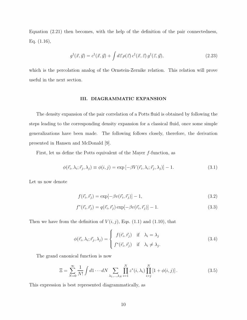
This expression is best represented diagrammatically, as

10

Ξ = 1 + t + t t + t t +t t

t

+t t

t

+

t t

t

T

T +t t

t

T

T + . . . (3.6)

In these diagrams, each circle corresponds to a function z∗(i, λi), and is therefore associated

with a discrete spin variable as well as with a position coordinate. Each line corresponds to

φ(i, j). For each black circle, we integrate over the space coordinate and sum over the spin

coordinate. For example,

t t =∫

d~ri d~rj

∑

λi

∑

λj

z∗(~ri, λi) z∗(~rj, λj)φ(~ri, λi;~rj , λj). (3.7)

We will also have white circles over which there is neither integration nor summation. Note,

finally, that the symmetry factor of the diagrams, being a purely combinatorial quantity, is

the same here as for the usual diagrams without spin variables. While this is not necessarily

so when the lines can stand for different functions as they can here, nevertheless it remains

true because the identity of the lines is uniquely determined by spin variables which are then

summed upon.

It is now easy to see that all the usual definitions and theorems which hold for the

usual spinless diagrams hold also for the spin diagrams introduced here. In particular, the

Morita-Hiroike lemmas (see, e.g., Hansen and McDonald [9]) hold here as well, provided the

functional derivatives which appear in them are generalized to be the spin-functional deriva-

tives introduced in the previous section. For example, we have the following generalized

lemma.

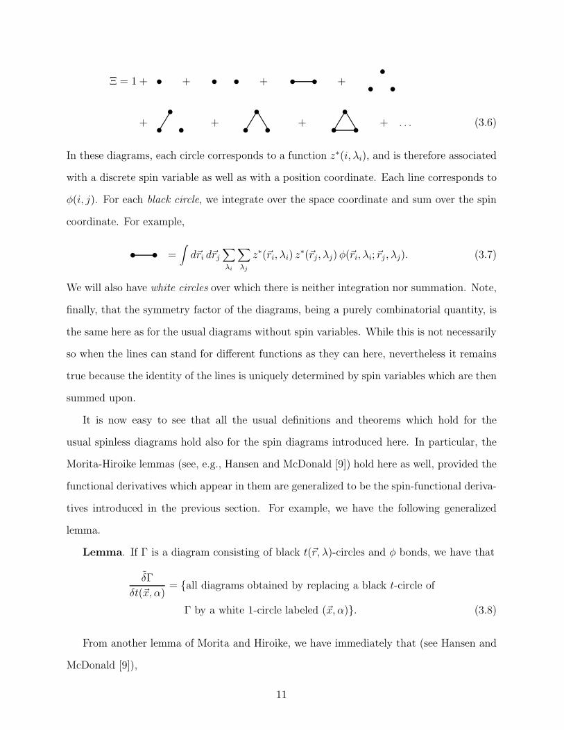
Lemma. If Γ is a diagram consisting of black t(~r, λ)-circles and φ bonds, we have that

δΓ

δt(~x, α)= all diagrams obtained by replacing a black t-circle of

Γ by a white 1-circle labeled (~x, α). (3.8)

From another lemma of Morita and Hiroike, we have immediately that (see Hansen and

McDonald [9]),

11

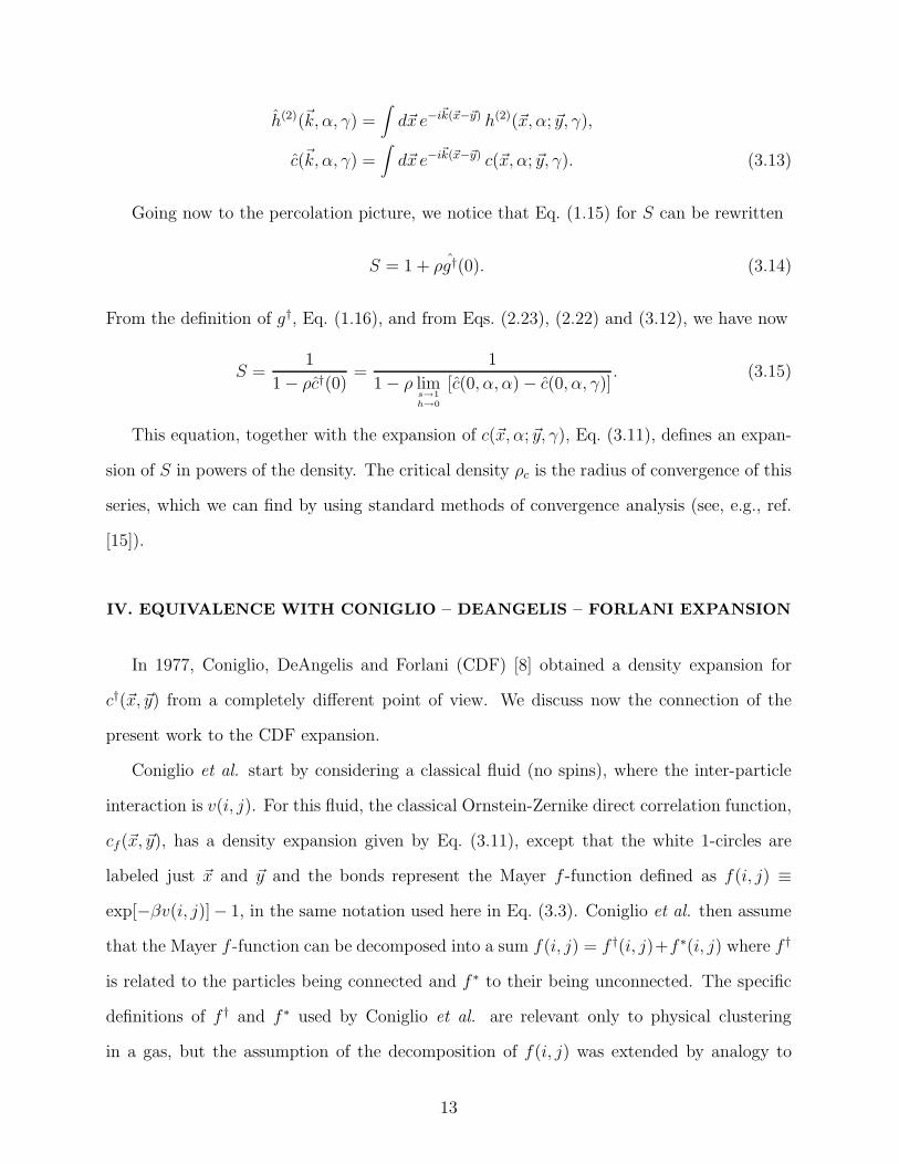
ln Ξ = all simple connected diagrams consisting of black z∗-circles and φ-bonds

= t + t t +t t

t

T

T +t t

t

T

T + . . . , (3.9)

from which we can show that

ln[

ρ(1)(~x, α)/z∗(~x, α)]

= all simple diagrams consisting of one white

1-circle labeled (~x, α), one or more black

ρ(1)-circles and φ bonds, such that they are

free of connecting circles. (3.10)

A connecting circle is a circle the removal of which (along with the bonds which emerge

from it) causes the diagram to become disconnected.

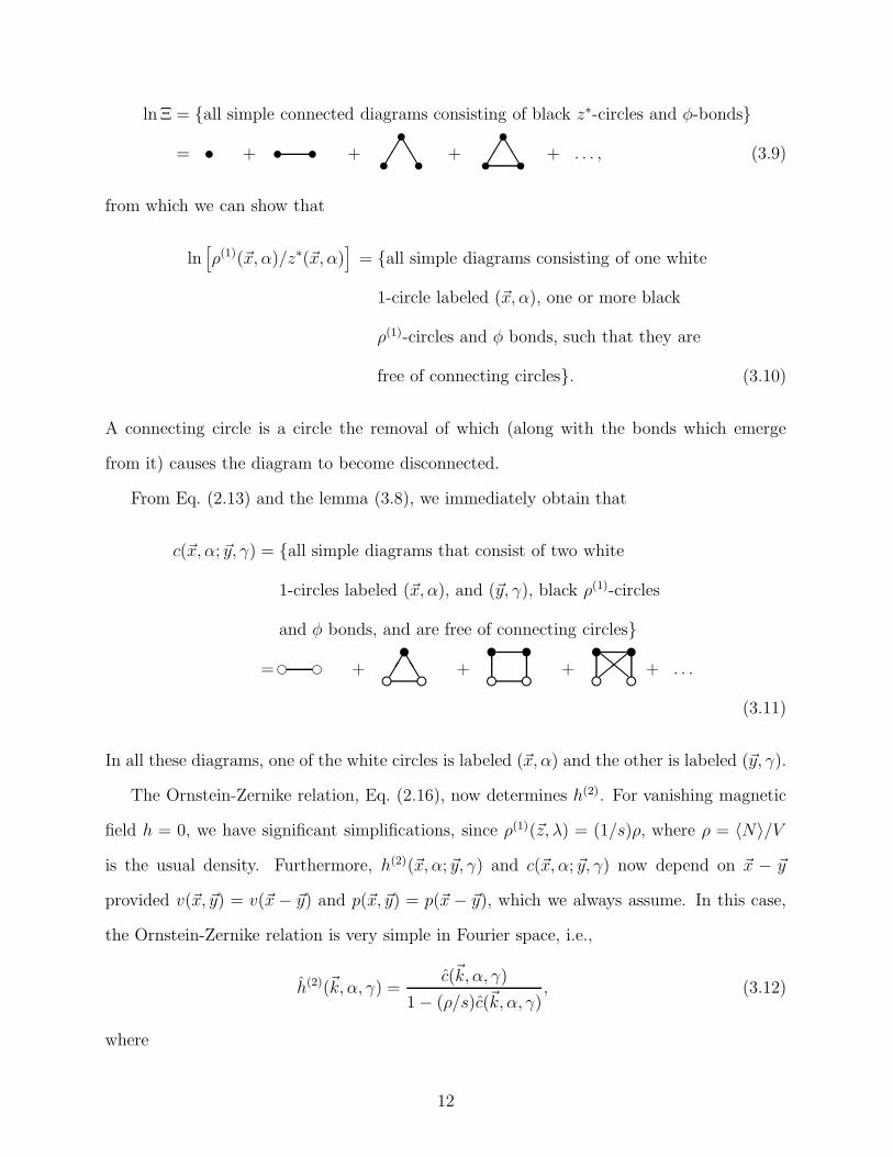
From Eq. (2.13) and the lemma (3.8), we immediately obtain that

c(~x, α; ~y, γ) = all simple diagrams that consist of two white

1-circles labeled (~x, α), and (~y, γ), black ρ(1)-circles

and φ bonds, and are free of connecting circles

= e e +e e

u

TT +

e e

u u

+e e

u u

,,ll + . . .

(3.11)

In all these diagrams, one of the white circles is labeled (~x, α) and the other is labeled (~y, γ).

The Ornstein-Zernike relation, Eq. (2.16), now determines h(2). For vanishing magnetic

field h = 0, we have significant simplifications, since ρ(1)(~z, λ) = (1/s)ρ, where ρ = 〈N〉/V

is the usual density. Furthermore, h(2)(~x, α; ~y, γ) and c(~x, α; ~y, γ) now depend on ~x − ~y

provided v(~x, ~y) = v(~x − ~y) and p(~x, ~y) = p(~x − ~y), which we always assume. In this case,

the Ornstein-Zernike relation is very simple in Fourier space, i.e.,

h(2)(~k, α, γ) =c(~k, α, γ)

1 − (ρ/s)c(~k, α, γ), (3.12)

where

12

h(2)(~k, α, γ) =∫

d~x e−i~k(~x−~y) h(2)(~x, α; ~y, γ),

c(~k, α, γ) =∫

d~x e−i~k(~x−~y) c(~x, α; ~y, γ). (3.13)

Going now to the percolation picture, we notice that Eq. (1.15) for S can be rewritten

S = 1 + ρg†(0). (3.14)

From the definition of g†, Eq. (1.16), and from Eqs. (2.23), (2.22) and (3.12), we have now

S =1

1 − ρc†(0)=

1

1 − ρ lims→1h→0

[c(0, α, α) − c(0, α, γ)]. (3.15)

This equation, together with the expansion of c(~x, α; ~y, γ), Eq. (3.11), defines an expan-

sion of S in powers of the density. The critical density ρc is the radius of convergence of this

series, which we can find by using standard methods of convergence analysis (see, e.g., ref.

[15]).

IV. EQUIVALENCE WITH CONIGLIO – DEANGELIS – FORLANI EXPANSION

In 1977, Coniglio, DeAngelis and Forlani (CDF) [8] obtained a density expansion for

c†(~x, ~y) from a completely different point of view. We discuss now the connection of the

present work to the CDF expansion.

Coniglio et al. start by considering a classical fluid (no spins), where the inter-particle

interaction is v(i, j). For this fluid, the classical Ornstein-Zernike direct correlation function,

cf(~x, ~y), has a density expansion given by Eq. (3.11), except that the white 1-circles are

labeled just ~x and ~y and the bonds represent the Mayer f -function defined as f(i, j) ≡

exp[−βv(i, j)]− 1, in the same notation used here in Eq. (3.3). Coniglio et al. then assume

that the Mayer f -function can be decomposed into a sum f(i, j) = f †(i, j)+f ∗(i, j) where f †

is related to the particles being connected and f ∗ to their being unconnected. The specific

definitions of f † and f ∗ used by Coniglio et al. are relevant only to physical clustering

in a gas, but the assumption of the decomposition of f(i, j) was extended by analogy to

13

other systems by several workers [3,10,11]. However, no formal basis was provided for the

definition of f † and f ∗ in the general case. If we take f ∗ as formally defined here in Eq. (3.3),

which is natural since this function is directly related to the probability of the two particles

being unconnected, we find that

f †(i, j) ≡ f(i, j) − f ∗(i, j) = p(i, j) exp [−βv(i, j)] . (4.1)

This result is satisfying since f † turns out to be directly proportional to the probability of

the two particles being connected.

Coniglio et al. then replace f in the diagrammatic expansion of cf (~x, ~y), with the sum

f † + f ∗, and consider all the decomposed diagrams thus obtained, in which every bond is

either an f † or an f ∗ function. The sum of all the diagrams which contain at least one

continuous path of f † functions between the white 1-circles, they consider to be c†(~x, ~y),

while the remainder is called c∗(~x, ~y), so that cf (~x, ~y) = c†(~x, ~y) + c∗(~x, ~y).

It is hardly obvious now that this algorithm agrees with the expansion obtained here.

Indeed, the function f † never appears in the present expansion. Nonetheless, the two for-

mulations are equivalent.

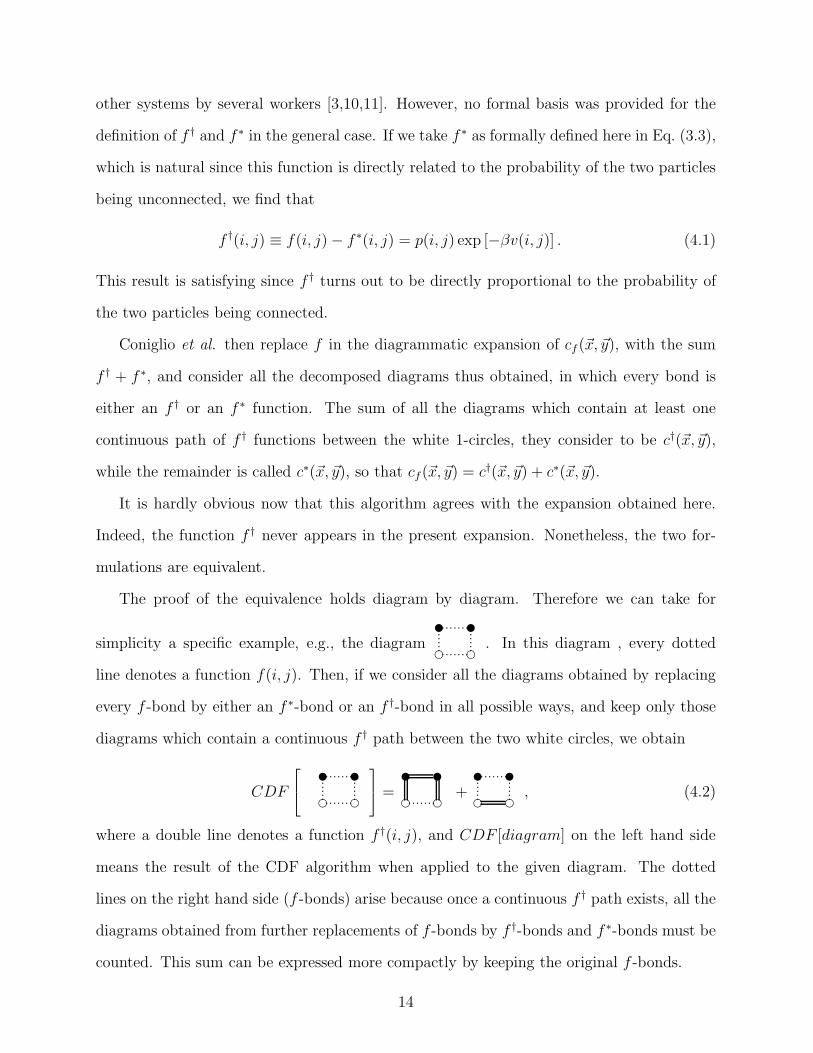
The proof of the equivalence holds diagram by diagram. Therefore we can take for

simplicity a specific example, e.g., the diagrame e

u u

p p p p p p p

p p p p p p p

ppppppp

ppppppp

. In this diagram , every dotted

line denotes a function f(i, j). Then, if we consider all the diagrams obtained by replacing

every f -bond by either an f ∗-bond or an f †-bond in all possible ways, and keep only those

diagrams which contain a continuous f † path between the two white circles, we obtain

CDF

e e

u u

p p p p p p p

p p p p p p p

ppppppp

ppppppp

=e e

u u

p p p p p p p+

e e

u up p p p p p p

ppppppp

ppppppp

, (4.2)

where a double line denotes a function f †(i, j), and CDF [diagram] on the left hand side

means the result of the CDF algorithm when applied to the given diagram. The dotted

lines on the right hand side (f -bonds) arise because once a continuous f † path exists, all the

diagrams obtained from further replacements of f -bonds by f †-bonds and f ∗-bonds must be

counted. This sum can be expressed more compactly by keeping the original f -bonds.

14

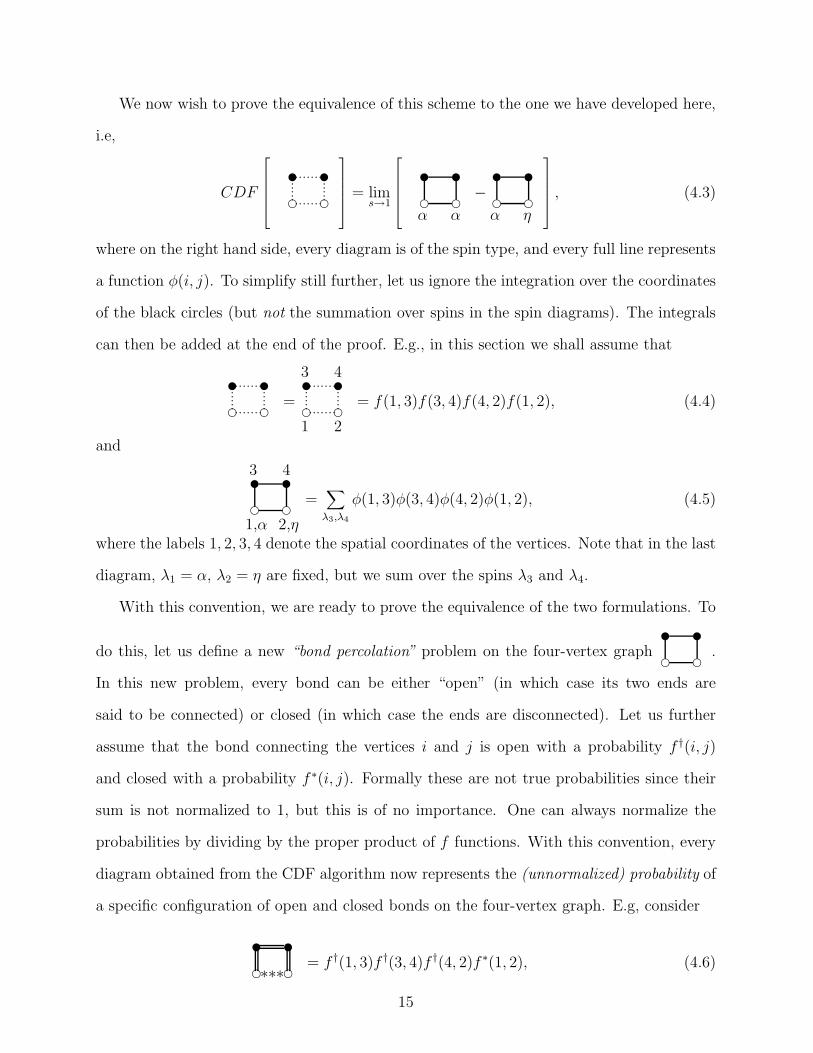
We now wish to prove the equivalence of this scheme to the one we have developed here,

i.e,

CDF

e e

u u

p p p p p p p

p p p p p p p

ppppppp

ppppppp

= lims→1

e e

u u

α α

−e e

u u

α η

, (4.3)

where on the right hand side, every diagram is of the spin type, and every full line represents

a function φ(i, j). To simplify still further, let us ignore the integration over the coordinates

of the black circles (but not the summation over spins in the spin diagrams). The integrals

can then be added at the end of the proof. E.g., in this section we shall assume that

e e

u u

p p p p p p p

p p p p p p p

ppppppp

ppppppp

=e e

u u

p p p p p p p

p p p p p p p

ppppppp

ppppppp

1 2

3 4

= f(1, 3)f(3, 4)f(4, 2)f(1, 2), (4.4)

and

e e

u u

1,α 2,η

3 4

=∑

λ3,λ4

φ(1, 3)φ(3, 4)φ(4, 2)φ(1, 2), (4.5)

where the labels 1, 2, 3, 4 denote the spatial coordinates of the vertices. Note that in the last

diagram, λ1 = α, λ2 = η are fixed, but we sum over the spins λ3 and λ4.

With this convention, we are ready to prove the equivalence of the two formulations. To

do this, let us define a new “bond percolation” problem on the four-vertex graphe e

u u

.

In this new problem, every bond can be either “open” (in which case its two ends are

said to be connected) or closed (in which case the ends are disconnected). Let us further

assume that the bond connecting the vertices i and j is open with a probability f †(i, j)

and closed with a probability f ∗(i, j). Formally these are not true probabilities since their

sum is not normalized to 1, but this is of no importance. One can always normalize the

probabilities by dividing by the proper product of f functions. With this convention, every

diagram obtained from the CDF algorithm now represents the (unnormalized) probability of

a specific configuration of open and closed bonds on the four-vertex graph. E.g, consider

e e

u u

∗∗∗= f †(1, 3)f †(3, 4)f †(4, 2)f ∗(1, 2), (4.6)

15

where a line of ∗ represents a function f ∗. The same diagram can also be thought of as a

configuration of open and closed bonds on the four-vertex graph, by letting a double line

represent an open bond and a ∗-line a closed bond. This geometrical configuration occurs

with a probability f †(1, 3)f †(3, 4)f †(4, 2)f ∗(1, 2), which is just the value of the equivalent

diagram, Eq. (4.6). Every diagram therefore functions in a double capacity. On the one hand

it represents an actual configuration of open and closed bonds on some graph. On the other

hand, it represents some functional value. This functional value is just the (unnormalized)

probability of the bond configuration represented by the same graph.

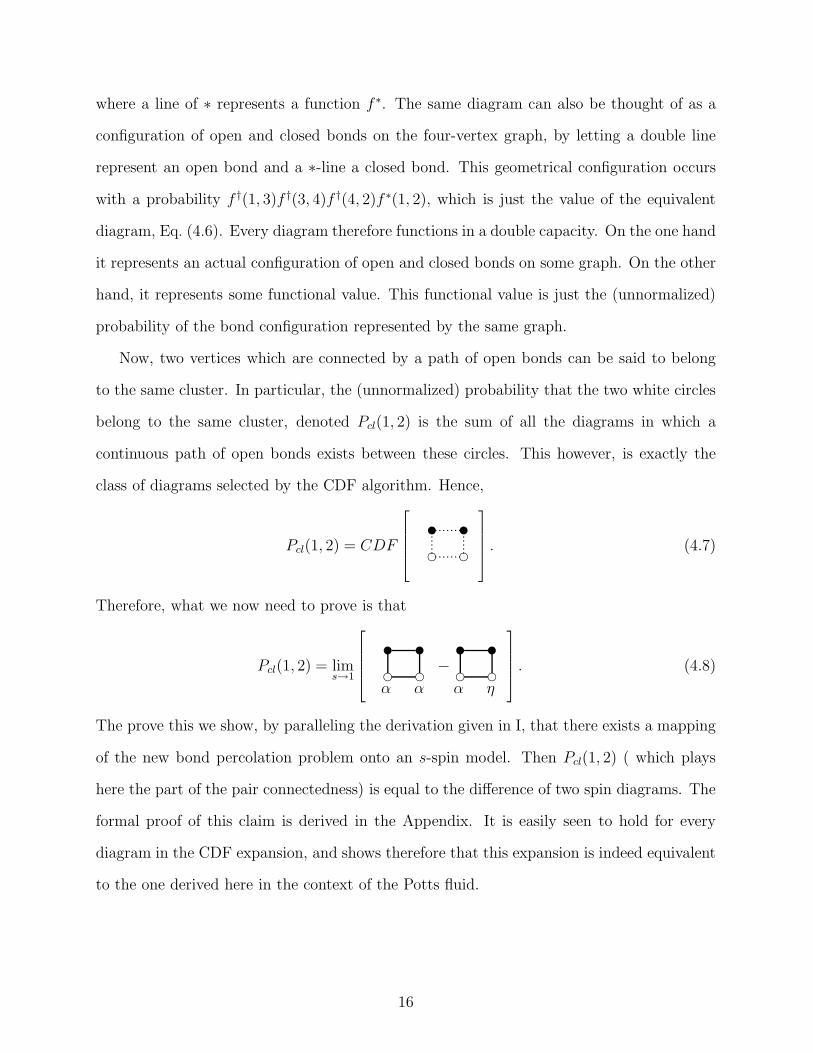
Now, two vertices which are connected by a path of open bonds can be said to belong

to the same cluster. In particular, the (unnormalized) probability that the two white circles

belong to the same cluster, denoted Pcl(1, 2) is the sum of all the diagrams in which a

continuous path of open bonds exists between these circles. This however, is exactly the

class of diagrams selected by the CDF algorithm. Hence,

Pcl(1, 2) = CDF

e e

u u

p p p p p p p

p p p p p p p

ppppppp

ppppppp

. (4.7)

Therefore, what we now need to prove is that

Pcl(1, 2) = lims→1

e e

u u

α α

−e e

u u

α η

. (4.8)

The prove this we show, by paralleling the derivation given in I, that there exists a mapping

of the new bond percolation problem onto an s-spin model. Then Pcl(1, 2) ( which plays

here the part of the pair connectedness) is equal to the difference of two spin diagrams. The

formal proof of this claim is derived in the Appendix. It is easily seen to hold for every

diagram in the CDF expansion, and shows therefore that this expansion is indeed equivalent

to the one derived here in the context of the Potts fluid.

16

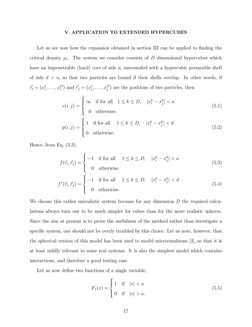
V. APPLICATION TO EXTENDED HYPERCUBES

Let us see now how the expansion obtained in section III can be applied to finding the

critical density ρc. The system we consider consists of D dimensional hypercubes which

have an impenetrable (hard) core of side a, surrounded with a hypercubic permeable shell

of side d > a, so that two particles are bound if their shells overlap. In other words, if

~ri = (x1i , . . . , x

Di ) and ~rj = (x1

j , . . . , xDj ) are the positions of two particles, then

v(i, j) =

∞ if for all 1 ≤ k ≤ D, |xki − xk

j | < a

0 otherwise.(5.1)

p(i, j) =

1 if for all 1 ≤ k ≤ D, |xki − xk

j | < d

0 otherwise.(5.2)

Hence, from Eq. (3.3),

f(~ri, ~rj) =

−1 if for all 1 ≤ k ≤ D, |xki − xk

j | < a

0 otherwise.(5.3)

f ∗(~ri, ~rj) =

−1 if for all 1 ≤ k ≤ D, |xki − xk

j | < d

0 otherwise.(5.4)

We choose this rather unrealistic system because for any dimension D the required calcu-

lations always turn out to be much simpler for cubes than for the more realistic spheres.

Since the aim at present is to prove the usefulness of the method rather than investigate a

specific system, one should not be overly troubled by this choice. Let us note, however, that

the spherical version of this model has been used to model microemulsions [3], so that it is

at least mildly relevant to some real systems. It is also the simplest model which contains

interactions, and therefore a good testing case.

Let us now define two functions of a single variable,

F1(x) =

1 if |x| < a

0 if |x| > a.(5.5)

17

F2(x) =

1 if |x| < d

0 if |x| > d.(5.6)

The equations (5.4) can now be rewritten as

f(x1, . . . , xD) = −D∏

i=1

F1(xi). (5.7)

f ∗(x1, . . . , xD) = −D∏

i=1

F2(xi). (5.8)

We shall now calculate c† up to the second order in ρ (i.e., up to square diagrams). The

zeroth order is

lims→1

[

e e

α α− e e

α γ

]

=∫

d~z [f(~z) − f ∗(~z)] = dD(

1 − ηD)

, (5.9)

where we have defined the aspect ratio, η, as

η ≡a

d. (5.10)

For the first order (triangular diagrams), we need, e.g., the integral

Ω(~y) ≡∫

d~x f(~x) f(~x− ~y) =D∏

i=1

∫

dxi F1(xi)F1(x

i − yi)

. (5.11)

It is precisely the factorization of this and similar integrals into a product of identical one

dimensional integrals that is the main simplification afforded by the use of a cubic geometry.

As a beneficial side-effect, it allows us to check the influence of system dimensionality on

the critical density.

Ω(~y) is very simple to evaluate when we realize that∫

dxF1(x)F1(x − y) is merely the

overlap of two segments of length a, one of which is centered at the origin, the other centered

at the position y. By direct inspection, we have therefore that

∫

dxF1(x)F1(x− y) =

2a− |y| if |y| < 2a

0 if |y| > 2a, (5.12)

∫

dxF2(x)F2(x− y) =

2d− |y| if |y| < 2d

0 if |y| > 2d, (5.13)

18

∫

dxF1(x)F2(x− y) =

2a if |y| < d− a

d+ a− |y| if d− a < |y| < d+ a

0 if |y| > d+ a

. (5.14)

Let us consider a typical contribution from the triangular diagrams, e.g., the integral

∫

dx dy F2(x)F2(x − y)F1(y). In this integral, we interpret the term F1(y) as merely spec-

ifying the limits of integration, i.e., determining that |y| < a. Since d > a, we have from

Eq. (5.13) that

∫

dx dy F2(x)F2(x− y)F1(y) =∫ a

−ady[∫

dxF2(x)F2(x− y)]

= 4da− a2. (5.15)

All the required one dimensional integrals can now be calculated along the same lines. In

fact, equations (5.12)–(5.14) suffice to calculate all the triangular and square diagrams,

except for the last fully connected square diagram which is a product of six F functions.

For this diagram the previous arguments have to be generalized but it can be done easily

along the lines already presented.

All the integrals we need are presented in Tables I–IV. The first column in each table

contains the notation of the integral, and the third column its value. All these integrals are

D-th powers of some one dimensional integrals, [see, e.g., Eq. (5.11)]. The corresponding

one-dimensional integrals appear in the second column.

We now have, after some straightforward calculations, that the contribution of the tri-

angular diagrams, denoted (2d)2D k2, is, in the notation of Tables I–IV,

(2d)2D k2 = I1 − 2 I2 + I3. (5.16)

Similarly, the contribution from the square diagrams is denoted (2d)3D k3, and in the

notation of Tables I–IV is equal to

(2d)3D k3 =3

2J1 − 5J2 + 5J3 −

3

2J4 − 3K1 + 3K2 −

1

2K3 + 7K4 − 10K5 +

7

2K6

+1

2L1 − L2 − L3 +

5

2L4 − L5. (5.17)

Substituting these results into Eq. (3.15) yields, for the mean cluster size,

19

S =1

1 − ρdD (1 − ηD) − ρ2(2d)2Dk2 − ρ3(2d)3Dk3 +O(ρ4). (5.18)

The critical density is commonly measured in dimensionless units. Let us define

B = (2d)Dρ, (5.19)

which is chosen to reduce to the total excluded volume when a → 0 [7]. As mentioned in

the introduction, this reduces the dependence of the density on the details of the system

and facilitates the presentation of the results. Finally, using standard methods [16], we find

the series expansion for the mean cluster size to be

S = 1 + S1B + S2B2 + S3B

3 +O(B4), (5.20)

with

S1 =1 − ηD

2D,

S2 = k2 + S21 ,

S3 = k3 + 2S1k2 + S31 . (5.21)

VI. RESULTS FOR HYPERCUBES

To find the critical density, we need some extrapolation method which will yield the point

of divergence of the series (5.20). Unfortunately, we know very few terms in this series. The

results can be improved, however, by using additional information. In particular, S diverges

as S ∼ (Bc −B)−γ , and γ appears to be universal, i.e., independent of the interaction, and

furthermore, equal to the well known value it takes in lattice percolation. Biased methods

use the known value of γ to calculate Bc. There are several methods available, but for the

present use, the best seems to be the one developed by Arteca, Fernandez, and Castro (AFC)

[17]. The biased version of this method relies on the fact that the function (Bc − B)γS(B)

is analytical around Bc. Therefore, we define a function of two variables,

20

g(u,B) =(

1 −B

u

)γ

S(B), (6.1)

where we have assumed a known value for γ. Given an expansion S =∑

SnBn, we can

expand g(u,B) in powers of B, with the result,

g(u,B) =∞∑

n=0

gn(u)Bn, (6.2)

where

gn(u) =n∑

k=0

(

γ

k

)

(−u)−kSn−k. (6.3)

Since g(u,B) is analytical at u = Bc, the idea is now to look for values of u which maximize

the convergence of the series gn(u)∞n=1 as n → ∞. The AFC proposal is to generate a

series un∞n=1 of solutions of the equation

gn(un) = 0. (6.4)

Then we expect that

limn→∞

un = Bc. (6.5)

In the case of the series (5.20), we know the terms only up to n = 3, which is too little to

extrapolate a reliable limit to the series un∞n=1. Therefore, we take simply the last term of

the series , u3, as our estimate of Bc.

In figures (1)–(5), we compare this theoretical estimate to results of computer simula-

tions for dimensions 2, 3, 4 and 5, as a function of the aspect ratio η. The simulations were

performed with an efficient new algorithm we introduced recently for investigating contin-

uum percolation with interactions [18]. Unlike the usual Metropolis algorithm, this method

increases serially the density in the system until percolation is achieved. The effect of the

interactions is included through a rejection criterion which produces an effective statistical

weight for the configurations. The final (percolating) configuration contained close to 30,000

particles in two and three dimensions and around 10,000 in the higher dimensions. The re-

sults are averages over 10 independent runs and the numerical error is estimated to range

from 5% to 10 %.

21

Let us first consider the well reproduced qualitative behavior of Bc(η). The main features

can be understood from simple arguments. As pointed out by Bug et al. [3], the minimum

of Bc(η) results from the competition between two processes. As the diameter of the hard

core increases, it becomes harder to bring particles close enough to each other for them to

bind. This effect clearly dominates at high η. At low η, on the other hand, the hard core

is much too small relative to the soft shell to prevent binding significantly, but it increases

the average distance between bound particles. As a result the clusters are “longer”, and

therefore percolate “sooner”, hence Bc is lower.

The dependence on D is understandable in terms of the ratio of the permeable shell vol-

ume to the hard core volume. Clearly, this ratio increases with the dimensionality. Therefore,

at any given η, the influence of the hard core diminishes as D increases. As a result, the

graph of Bc(η) looks flatter, while the influence of the final singularity at η = 1 (at which

there is no possibility of binding anymore and therefore no percolating phase), is limited to

regions of higher η. This influences also the feasibility of the simulations. Clearly, the larger

the hard core, i.e., the greater η, the harder it is to simulate the system. Hence, e.g., in

two dimensions, we have no results beyond η = 0.8 due to this difficulty. As D increases,

however, higher η become more accessible. Unfortunately, it is generally harder to simulate

high dimensional systems, which is why we stopped at D = 5. The trends, however, are

obvious, and there should be nothing exceptional for D > 5.

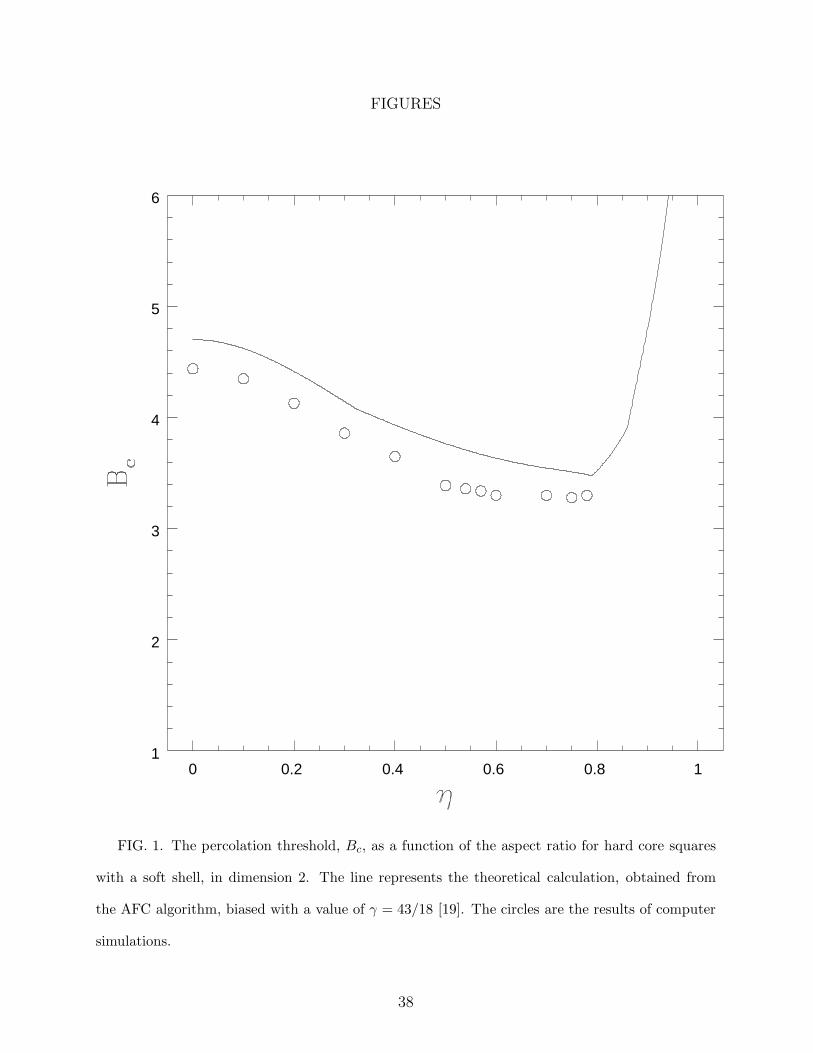
Turning now to the detailed comparison between theory and simulations, we see that

the results are quantitatively close to each other. Even in the worse case, in two dimensions

(Fig. 1), the difference between theory and simulations is at most 11% (at η = 0.5). The

position of the minimum, theoretically predicted to be η = 0.79, also agrees well with the

simulations.

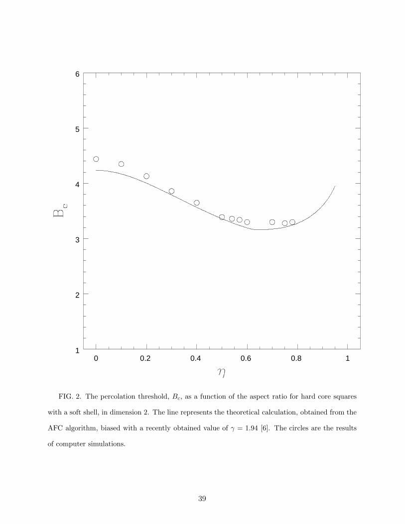
Very recently, however, Okazaki et al. [6] have performed new simulations of two dimen-

sional continuum percolation, and claim that the critical exponents are in fact different from

those of lattice percolation. For the exponent γ they find γ = 1.94 instead of the higher

43/18 obtained in lattice percolation [19]. More work is certainly needed to resolve this

22

issue. Here we merely note the effects of such a shift in the value of γ on the theoretical

prediction. Figure 2 presents the results obtained in two dimensions when the value of γ

found by Okazaki et al. is used for the biasing. The fit is quite improved by this change. Un-

fortunately the approximations we use are too drastic to claim that our calculations actually

support the value obtained by Okazaki et al.. But they do suggest that the question of the

universality class of continuum percolation is not yet settled and requires more investigation.

Note however that the relative change in Bc is smaller than the change in γ which

produced it. Therefore, Bc is not extremely sensitive to the value of the bias. Since other

simulations find values of γ in higher dimensions which are at least close to the values

obtained in lattice percolation, we may use these lattice values for the bias and expect that

Bc will not be affected notably. For this reason and for lack of other data on the value of γ

in continuum percolation, we therefore use the accepted lattice values for dimensions higher

than two.

In three dimensions, up to η = 0.8, the greatest discrepancy between theory and “ex-

periment” is only 4 %, well within the limits of the simulation error. Even at η = 0.8, the

largest discrepancy we have, the deviation is only about 6 %, still within the simulation error

(which increases slightly with η because of the above mentioned problems in performing the

simulations in the vicinity of η = 1).

This trend continues in dimension 4, where the discrepancy between the theory and the

simulations remains below 6 % until η = 0.65, and in dimension 5. Note, however, that

as a general rule simulation errors increase with dimensionality due to the greater difficulty

in performing the simulations, and therefore comparison with the theory becomes slightly

more problematic. In particular, at D = 5 there seems to be a systematic discrepancy with

the theory which could well reflect some finite size scaling effects in the simulations. It

is therefore quite possible that the theory is actually more precise at this point than the

simulations.

Considering that we use the series for S only up to second order, the quantitative agree-

ment obtained is a remarkable success for the theory.

23

VII. DISCUSSION

We have seen how the Potts fluid mapping allows us to derive a general expansion in

powers of the density for the mean cluster size and the pair connectedness. This expansion

can be used to calculate the percolation threshold by calculating the first terms in the series

then using some extrapolation method to find the radius of convergence of the series. We

have applied this scheme to interacting hypercubes in dimensions ranging from 2 to 5, and

we have shown that even with merely three terms in the series we already obtain very good

quantitative results, within a few percents of the results of the computer simulations.

Ours is not the first work to use density expansions of the mean cluster size, obtained in

one way or another (e.g., from an analogy with lattice systems [21]), but it is the first one to

derive quantitatively adequate results for interacting systems. We believe this success stems

from a simple but fundamental reason.

When Coniglio et al. [8] obtained their expansion of S, they did not use it directly to

calculate the critical density. Instead, they turned for inspiration to the theory of liquids and

considered the integral equations for the pair correlation which had proved successful there,

primarily the Percus- Yevick (PY) equation. Coniglio et al. derived a percolative analog of

this equation by applying the CDF algorithm to its diagrammatic expansion. Some time

later, De Simone et al. [10] applied this equation to a system of extended spheres, the spher-

ical analog of the system investigated in the present work. The results were qualitatively

correct but quantitatively poor. Discrepancies between theory and simulations ranged from

40 % to no less than 10 %. Several researchers [11] extended this work to other interactions

or shapes with always the same quantitatively inadequate results. We believe this failure

holds a simple (in hindsight, in fact, obvious), but apparently under-appreciated lesson.

The guiding principle behind the work of Coniglio et al. and their followers seems to have

been viewing continuum percolation as a high density phenomenon. This is very reasonable

from a point of view which starts from the usual theory of fluids and then extracts the

percolative quantities from their normal fluid analogs. The CDF algorithm is explicitly

24

based on this point of view; given, e.g., the direct correlation function cf(~r) of the fluid, the

percolating part, c†(~r) can be extracted from it by looking at a diagrammatic expansion.

This means we need to know cf (~r) first. The percolation transition occurs at relatively high

densities, so that the normal fluid is either a dense gas or a liquid. In this case, integral

equations are the main tool for calculating the fluid’s properties, and therefore an adequate

starting point for obtaining the percolative properties as well.

But such a point of view misses the most important aspect of the percolation transition,

namely that it is a phase transition. Integral equations are known to describe the liquid well

only away from the liquid-gas critical point. As we approach the transition, they fail. The

quantitative failure of the percolative integral equations suggests that they suffer from an

analogous defect. There is direct evidence for this claim. Seaton and Glandt [22] checked

the mean cluster size for a wide range of densities and compared the predictions of integral

equations with the simulations. They found that the integral equations are indeed very

successful away from the critical density, but worsen steadily as ρ → ρc. In short, the

percolative integral equations behave with respect to the percolation transition exactly as

their analog in liquids behave with respect to the liquid transition.

At first sight this seems puzzling. At ρc, the normal liquid is usually away from its own

critical point, and it is therefore well described by integral equations. Now the procedure

for extracting the percolative part from these equations involves no further approximations.

Why then, do we obtain a relatively bad approximation by extracting exactly the percolative

part from a very good approximation?

This is precisely the heart of the matter, which is the trivial observation that the phase

transition is entirely ruled by the singular part of the relevant functions. Integral equa-

tions tend to smooth out this singular part, as evidenced, for example, by their systematic

overestimation of the critical density [10]. This doesn’t matter for the description of the

liquid, because the singular part is small at these densities. However when we turn to the

percolative analog, the entire physics we are after lies precisely in this overly smoothed out

singular part.

25

To understand a singular behavior, we must use methods adapted to singular functions.

This is the simple but under-appreciated lesson from all the preceding. It requires us to

abandon the view of continuum percolation as primarily a high density process. The density

at which the transition takes place is irrelevant for the choice of descriptive tools, since it only

influences the analytical part of the function. The proper tools to describe the percolation

transition are not those which describe well high density systems, but rather those which

describe well other phase transitions.

The present work proceeds clearly from this point of view. The underlying normal liquid

plays no part in the description presented here. Nowhere does the function cf (~r) or any of

its parents appear. Instead, we have a mapping onto a Potts fluid, from which we calculate

all the relevant quantities. One important difference between this and the older point of

view is that the magnetic transition of the Potts fluid can be identified with the percolation

transition, since the two relevant order parameter are essentially the same. Therefore we are

forced from the outset to employ only methods which are useful for the description of the

magnetic phase transition. Indeed, integral equations are not a natural tool to use here since

they will clearly fail in the description of the Potts fluid. Instead, we rely on one of the best

tried methods in critical phenomena, namely, an expansion valid in the disordered phase

(high temperature usually, low density in the present case). A low density expansion makes

no sense from the point of view of percolation as a high-density phenomenon. Indeed, we

do not expect the actual value of S obtained from the truncated series to be even remotely

good. But what we look for is a failure of convergence, the appearance of a singularity, and

for this a truncated series can be singularly well adapted, as countless investigations of the

Ising model have shown repeatedly [15].

It is precisely because the mapping onto a Potts fluid identifies one phase transition

(percolation) with another (magnetic) that we can achieve a remarkable quantitative agree-

ment between theory and simulations. Clearly, the truncated series expansion coupled with

an extrapolation method to find the radius of convergence is at present the best available

method to calculate theoretically the critical density in continuum percolation.

26

APPENDIX

We consider some diagram in the expansion, e.g., the example used in section IV,e e

u u

.

On this diagram we define a bond-percolation problem. We can now map the problem onto

a spin model by simply assigning to every vertex an s-spin, and assigning to every bond

between the vertices i and j a function φ(i, j) defined as in Eq. (3.1). We now proceed

to show, just as in paper I, that the bond-percolation model corresponds quantitatively

to the spin model. The result is again a geometrical mapping according to which every

percolation configuration corresponds to several spin configurations, in each of which all the

spins belonging to a single cluster are parallel. Different clusters, however, have randomly

assigned spin values. The following derivation parallels closely the one presented in paper I

for the continuum case.

Let the chosen diagram contain n vertices, and let us denote

Γ(1, 2, . . . , n) =∏

all existingbonds inthe graph

φ(i, j). (A1)

By convention, the two white circles are always labeled 1 and 2. The value associated with

the diagram in the spin model is therefore∑

λ3,λ4,...,λnΓ(1, . . . , n), where we assume that the

spins of the two white circles, λ1 and λ2, are fixed , and where we ignore the integration as

in section IV. The integration can be restored at the very end of the proof without changing

anything. For example, for the four-vertex graph mentioned above, we have

Γ(1, 2, 3, 4) = φ(1, 3)φ(3, 4)φ(4, 2)φ(2, 1). (A2)

Let us now select two spins, say λi and λj such that the bond φ(i, j) exists in the graph.

In the expression for Γ(1, . . . , n), let us separate all possible configurations λm into those

where λi = λj and the rest. Then,

∑

λm

Γ(1, . . . , n) = f(i, j)∑

λmλi=λj

Γ(1, . . . , n)

φ(i, j)+ f ∗(i, j)

∑

λmλi 6=λj

Γ(1, . . . , n)

φ(i, j). (A3)

27

We can rewrite the sum over the spins when λi 6= λj as the difference between the sum over

the spins without constraints and the sum over the spins when λi = λj, so that

∑

λm

Γ(1, . . . , n) = f †(i, j)∑

λmλi=λj

Γ(1, . . . , n)

φ(i, j)+ f ∗(i, j)

∑

λm

Γ(1, . . . , n)

φ(i, j). (A4)

where we used the relation f †(i, j) = f(i, j) − f ∗(i, j). The last sum∑

λm on the right

hand side is now performed over all spin configurations without constraints. Let us now

choose another pair of spins, say λi and λk (if such a bond exists). Repeating the previous

procedure, we obtain that

∑

λm

Γ(1, . . . , n) = f †(i, j) f †(i, k)∑

λmλi=λj=λk

Γ(1, . . . , n)

φ(i, j)φ(i, k)+ f †(i, j) f ∗(i, k)

∑

λmλi=λj

Γ(1, . . . , n)

φ(i, j)φ(i, k)

+ f ∗(i, j) f †(i, k)∑

λmλi=λk

Γ(1, . . . , n)

φ(i, j)φ(i, k)+ f ∗(i, j) f ∗(i, k)

∑

λm

Γ(1, . . . , n)

φ(i, j)φ(i, k). (A5)

This argument can be easily generalized to all pairs of spins. Let us consider one of the

sums into which the function∑

λmΓ(1, . . . , n) has been decomposed a step before, and con-

sider a pair (m,n) such that the bond φ(m,n) exists in the chosen diagram. Two possibilities

arise:

1. Previous constraints already determine that λm = λn (for example, there could be

some p for which λm = λp and λn = λp). Then,

∑

λm

previousconstraints

Γ(1, . . . , n)

φ(i, j) · · ·φ(l, k)= f †(m,n)

∑

λmprev.

constr.

Γ(1, . . . , n)

φ(i, j) · · ·φ(l, k)φ(m,n)

+ f ∗(m,n)∑

λmprev.

constr.

Γ(1, . . . , n)

φ(i, j) · · ·φ(l, k)φ(m,n), (A6)

where we have used the fact that if λm = λn, then φ(m,n) = f †(m,n) + f ∗(m,n).

2. Previous constraints do not determine that λm = λn. Then the situation is as it was

for the pair (i, j), and the sum will split in the following way

28

∑

λm

constr.

Γ(1, . . . , n)

φ(i, j) · · ·φ(l, k)= f †(m,n)

∑

λm: ...λm=λn

Γ(1, . . . , n)

φ(i, j) · · ·φ(l, k)φ(m,n)

+ f ∗(m,n)∑

λm: ...

Γ(1, . . . , n)

φ(i, j) · · ·φ(l, k)φ(m,n), (A7)

where in the second term on the right hand side no new constraint has been introduced.

The geometrical mapping follows because in case (2), every time a factor f † appears,

we have a new constraint forcing the two spins to be parallel. On the other hand, in the

percolation model, such a factor implies that the two vertices are connected, and therefore

belong to the same cluster. When a factor f ∗ appears, no new constraint is added, so that

the two vertices can be assigned spins at random. In case (1), on the other hand, the two

spins are already forced to be parallel by virtue of some previous constraints. According

to the foregoing argument, this means that they are both connected (at least indirectly) to

some other spin and therefore that they already belong to the same cluster. In this case it

does not matter anymore whether these vertices are also linked directly (a factor f †) or not

(a factor f ∗). Hence, we see that vertices which belong to the same cluster in the percolation

picture must be assigned parallel spins while the clusters themselves have randomly assigned

spin values.

When all pairs have been covered, the set of constraints of a particular sum specifies

exactly which particles belongs to which clusters in the original bond-percolation model

configuration. Since the expression for∑

λmΓ(1, . . . , n) contains sums over all possible con-

straints, it can be rewritten as a sum over all possible clusterings of the original percolation

configuration. Thus, let us define

P ( conn.) ≡∏

allboundpairs

(i,j)

f †(i, j)∏

allunbound

pairs(m,n)

f ∗(m,n). (A8)

Then we can write that

29

∑

λm

Γ(1, . . . , n) =∑

all possibleconnectivity

states

∑

λm consistentwith the

connectivitystate

P ( conn.) (A9)

where the sum over all spins is consistent with the connectivity state in the sense of the

geometrical mapping, i.e., that all vertices within a single cluster must be assigned the same

spin.

If we now assume that two vertices are connected with an unnormalized probability

f † and disconnected with an unnormalized probability f ∗ (see section IV), we have the

interpretation that P (conn.) is the unnormalized probability of finding a specific perco-

lation configuration of connected and disconnected vertices. Therefore, given a function

F (1, . . . , n) defined in the percolation model, of the coordinates of the vertices, we can

define its “average” as

〈F (1, . . . , n)〉p =∑

conn.states

P (conn.) F (1, . . . , n). (A10)

Similarly, we can have averages performed in the Potts fluid, which will be denoted by 〈 〉s.

Given a quantity G defined in the Potts fluid, we have

〈G(1, λ1; . . . ;n, λn)〉s =∑

λm

G(1, λ1; . . . ;n, λn)∏

i>j

φ(i, j). (A11)

Note that λ1 and λ2 are assumed fixed. Eq. (A9) now implies that in general, for any

quantity G(1, λ1; . . . ;n, λn) defined in the Potts fluid system, we have that

〈G(1, λ1; . . . ;n, λn)〉s =

⟨

∑

λm: cl

G(1, λ1; . . . ;n, λn)

⟩

p

, (A12)

where∑

λm: cl means a summation over all spin configurations which are consistent with

a given clustering in the sense of the geometrical mapping (i.e., such that all the spins in a

single cluster are parallel).

This fundamental relation allows us to relate to each other quantities in the percolation

model and quantities in the spin model. In particular, let us consider the function Ω(i, j)

defined in the percolation model as

30

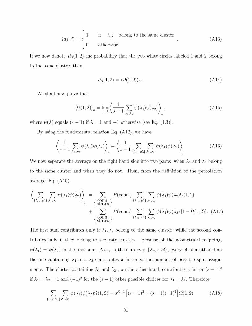
Ω(i, j) =

1 if i, j belong to the same cluster

0 otherwise. (A13)

If we now denote Pcl(1, 2) the probability that the two white circles labeled 1 and 2 belong

to the same cluster, then

Pcl(1, 2) = 〈Ω(1, 2)〉p. (A14)

We shall now prove that

〈Ω(1, 2)〉p = lims→1

⟨

1

s− 1

∑

λ1,λ2

ψ(λ1)ψ(λ2)

⟩

s

, (A15)

where ψ(λ) equals (s− 1) if λ = 1 and −1 otherwise [see Eq. (1.3)].

By using the fundamental relation Eq. (A12), we have

⟨

1

s− 1

∑

λ1,λ2

ψ(λ1)ψ(λ2)

⟩

s

=

⟨

1

s− 1

∑

λm: cl.

∑

λ1,λ2

ψ(λ1)ψ(λ2)

⟩

p

(A16)

We now separate the average on the right hand side into two parts: when λ1 and λ2 belong

to the same cluster and when they do not. Then, from the definition of the percolation

average, Eq. (A10),

⟨

∑

λm: cl.

∑

λ1,λ2

ψ(λ1)ψ(λ2)

⟩

p

=∑

conn.states

P (conn.)∑

λm: cl.

∑

λ1,λ2

ψ(λ1)ψ(λ2)Ω(1, 2)

+∑

conn.states

P (conn.)∑

λm: cl.

∑

λ1,λ2

ψ(λ1)ψ(λ2) [1 − Ω(1, 2)] . (A17)

The first sum contributes only if λ1, λ2 belong to the same cluster, while the second con-

tributes only if they belong to separate clusters. Because of the geometrical mapping,

ψ(λ1) = ψ(λ2) in the first sum. Also, in the sum over λm : cl, every cluster other than

the one containing λ1 and λ2 contributes a factor s, the number of possible spin assign-

ments. The cluster containing λ1 and λ2 , on the other hand, contributes a factor (s− 1)2

if λ1 = λ2 = 1 and (−1)2 for the (s− 1) other possible choices for λ1 = λ2. Therefore,

∑

λm: cl.

∑

λ1,λ2

ψ(λ1)ψ(λ2)Ω(1, 2) = sK−1[

(s− 1)2 + (s− 1)(−1)2]

Ω(1, 2) (A18)

31

where K is the total number of clusters in the configuration. Hence,

∑

conn.states

P (conn.)

s− 1

∑

λm: cl.

∑

λ1,λ2

ψ(λ1)ψ(λ2)Ω(1, 2) =∑

conn.states

P (conn.)sK−1(s− 1 + 1)Ω(1, 2)

=⟨

sKΩ(λ1, λ2)⟩

p. (A19)

The second term on the right hand side of Eq. (A17) contributes only if λ1, λ2 belong

to different clusters. The cluster containing λ1 contributes a factor (s − 1) if λ1 = 1, and

a factor (−1) in all the other (s − 1) cases. The same holds for the cluster containing λ2.

The K − 2 remaining clusters contribute each a factor s. Since the values of λ1 and λ2 are

assigned independently of each other, we have that

∑

λm: cl.

∑

λ1,λ2

ψ(λ1)ψ(λ2) [1 − Ω(1, 2)] = sK−2 [(s− 1) + (s− 1)(−1)]2 [1 − Ω(1, 2)] = 0.

(A20)

Combining Eq. (A19) and (A20), we see that

lims→1

⟨

1

s− 1

∑

λ1,λ2

ψ(λ1)ψ(λ2)

⟩

s

= 〈Ω(1, 2)〉p . (A21)

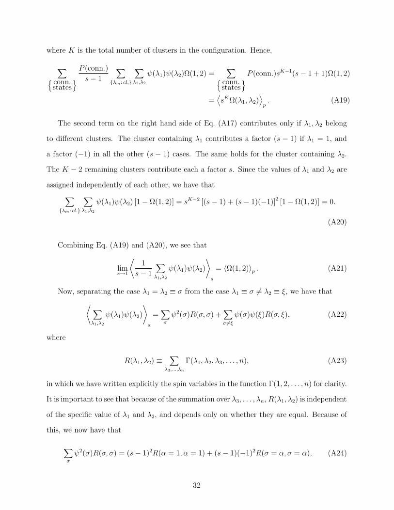
Now, separating the case λ1 = λ2 ≡ σ from the case λ1 ≡ σ 6= λ2 ≡ ξ, we have that

⟨

∑

λ1,λ2

ψ(λ1)ψ(λ2)

⟩

s

=∑

σ

ψ2(σ)R(σ, σ) +∑

σ 6=ξ

ψ(σ)ψ(ξ)R(σ, ξ), (A22)

where

R(λ1, λ2) ≡∑

λ3,...,λn

Γ(λ1, λ2, λ3, . . . , n), (A23)

in which we have written explicitly the spin variables in the function Γ(1, 2, . . . , n) for clarity.

It is important to see that because of the summation over λ3, . . . , λn, R(λ1, λ2) is independent

of the specific value of λ1 and λ2, and depends only on whether they are equal. Because of

this, we now have that

∑

σ

ψ2(σ)R(σ, σ) = (s− 1)2R(α = 1, α = 1) + (s− 1)(−1)2R(σ = α, σ = α), (A24)

32

where α is some arbitrary value of the spin different from 1. The factor (s− 1) in the last

term on the right hand side represents the possible choices of this spin α 6= 1. As a result,

lims→1

1

s− 1

∑

σ

ψ2(σ)R(σ, σ) = lims→1

R(α, α) (A25)

where α 6= 1, but is otherwise arbitrary.

Similarly,

∑

σ 6=ξ

ψ(σ)ψ(ξ)R(σ, ξ) = (s− 1)2 [R(1, α) +R(α, 1)] + (s− 1)(s− 2)R(α, η), (A26)

where α 6= η are arbitrary values of the spin which are both different from 1. As a result,

lims→1

1

s− 1

∑

σ 6=ξ

ψ(σ)ψ(ξ)R(σ, ξ) = − lims→1

R(α, η). (A27)

Combining Eqs. (A25) and (A27) we have that

lims→1

⟨

1

s− 1

∑

λ1,λ2

ψ(λ1)ψ(λ2)

⟩

s

= lims→1

[R(α, α) − R(α, η)] . (A28)

where α, η 6= 1 and α 6= η. Comparing with Eqs. (A14), (A21) and (A23), we finally obtain

that

Pcl(1, 2) = lims→1

∑

λ3,...,λn

Γ(α, α, λ3, . . . , λn) −∑

λ3,...,λn

Γ(α, η, λ3, . . . , λn)

. (A29)

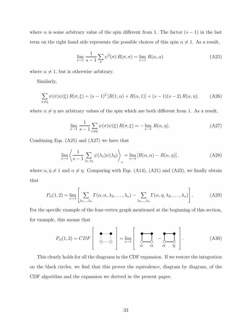
For the specific example of the four-vertex graph mentioned at the beginning of this section,

for example, this means that

Pcl(1, 2) = CDF

e e

u u

p p p p p p p

p p p p p p p

ppppppp

ppppppp

= lims→1

e e

u u

α α

−e e

u u

α η

. (A30)

This clearly holds for all the diagrams in the CDF expansion. If we restore the integration

on the black circles, we find that this proves the equivalence, diagram by diagram, of the

CDF algorithm and the expansion we derived in the present paper.

33

REFERENCES

[1] A. Drory, Phys. Rev. E 54, 5992 (1996); ibid., 54, 6003 (1996)

[2] For a review, see I. Balberg, Phil. Mag. B 55, 991 (1987).

[3] S. A. Safran, I. Webman and G. S. Grest, Phys. Rev. A 32, 506 (1985); A. L. R. Bug,

S.A. Safran, G. S. Grest and I. Webman, Phys. Rev. Lett. 55, 1896 (1985).

[4] G. Deutscher, in Disordered Systems and Localization, edited by C. Castellani, C. Di

Castro and L. Peliti (Springer-Verlag, Berlin, 1981).

[5] J. Texeira, in Correlations and Connectivity, edited by H. E. Stanley and N. Ostrowsky

(Kluwer Academic, Dordrecht, 1990).

[6] A. Okazaki, K. Maruyama, K. Okumura, Y. Hasegawa, and S. Miyazama, Phys. Rev.

E 54, 3389 (1996)

[7] I. Balberg, C. H. Anderson, S. Alexander and N. Wagner, Phys. Rev. B 30, 3933 (1984).

[8] A. Coniglio, U. DeAngelis and A. Forlani, J. Phys. A 10, 1123 (1977).

[9] J. P. Hansen and I. R. McDonald, Theory of Simple Liquids, 2nd ed. (Academic, London,

1986).

[10] T. De Simone, R. M. Stratt and S. Demoulini, Phys. Rev. Lett. 56, 1140 (1986); T. De

Simone, S. Demoulini and R. M. Stratt, J. Chem. Phys. 85, 391 (1986).

[11] Y. C. Chiew and E. D. Glandt, J. Phys. A 16, 2599 (1983); S. C. Netemeyer and E. D.

Glandt, J. Chem. Phys. 85, 6054 (1986).

[12] U. Alon, A. Drory, and I. Balberg, Phys. Rev. A 42, 4634 (1990).

[13] A. Drory, I. Balberg, U. Alon, and B. Berkowitz, Phys. Rev. A 43, 6604 (1991).

[14] A. Drory, Phys. Rev. E, in press, available at cond-mat/9610062.

34

[15] H. E. Stanley, Introduction to Phase Transitions and Critical Phenomena (Oxford Uni-

versity, New York, 1971).

[16] E.g, M. Abramovitz and I. A. Stegun, Handbook of Mathematical Functions (Dover,

New York, 1968), p. 15.

[17] G. A. Arteca, F. M. Fernandez and E. A. Castro, Phys. Rev. A 33, 1297 (1986).

[18] A. Drory, B. Berkowitz, and I. Balberg, Phys. Rev. E 49, R949 (1994); ibid. 52, 4482

(1995).

[19] D. Stauffer and A. Aharony, Introduction to Percolation Theory, 2nd revised ed., (Taylor

and Francis, London, 1994).

[20] H. J. Herrmann and D. Stauffer, Z. Phys. B 44, 339 (1981).

[21] W. Haan and R. Zwanzig, J. Phys. A 10, 1547 (1977).

[22] N. A. Seaton and E. D. Glandt, J.Chem. Phys. 86, 4668 (1987); ibid. 87, 1785 (1987).

35

TABLES

TABLE I. The integrals contributed by triangular diagrams. The first column is the notation

and the last is the value. This value is the D–th power of the one dimensional integral whose

integrand occupies the second column.The variables x and y are integrated upon.

I1 F1(x)F1(x − y)F1(y) (3a2)D

I2 F2(x)F2(x − y)F1(y) (4da − a2)D

I3 F2(x)F2(x − y)F2(y) (3d2)D

TABLE II. The integrals contributed by square diagrams with four lines. The first column is

the notation and the last is the value. This value is the D–th power of the one dimensional integral

whose integrand occupies the second column. The variables x, y, and z are integrated upon.

J1 F1(x)F1(x − y)F1(z)F1(z − y)(

163 a3

)D

J2 F1(x)F1(x − y)F2(z)F2(z − y)(

8da2 − 13a3

)D

J3 F1(x)F2(x − y)F2(z)F2(z − y)(

6d2a − 23a3

)D

J4 F2(x)F2(x − y)F2(z)F2(z − y)(

163 d3

)D

36

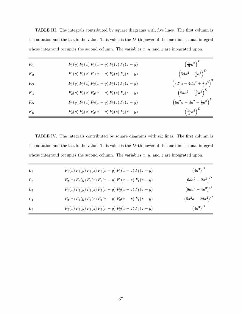
TABLE III. The integrals contributed by square diagrams with five lines. The first column is

the notation and the last is the value. This value is the D–th power of the one dimensional integral

whose integrand occupies the second column. The variables x, y, and z are integrated upon.

K1 F1(y)F1(x)F1(x − y)F1(z)F1(z − y)(

143 a3

)D

K2 F1(y)F1(x)F1(x − y)F2(z)F2(z − y)(

6da2 − 43a3

)D

K3 F1(y)F2(x)F2(x − y)F2(z)F2(z − y)(

8d2a − 4da2 + 23a3

)3

K4 F2(y)F1(x)F2(x − y)F1(z)F2(z − y)(

8da2 − 103 a3

)D

K5 F2(y)F1(x)F2(x − y)F2(z)F2(z − y)(

6d2a − da2 − 13a3

)D

K6 F2(y)F2(x)F2(x − y)F2(z)F2(z − y)(

143 d3

)D

TABLE IV. The integrals contributed by square diagrams with six lines. The first column is

the notation and the last is the value. This value is the D–th power of the one dimensional integral

whose integrand occupies the second column. The variables x, y, and z are integrated upon.

L1 F1(x)F1(y)F1(z)F1(x − y)F1(x − z)F1(z − y)(

4a3)D

L2 F2(x)F2(y)F2(z)F1(x − y)F1(x − z)F1(z − y)(

6da2 − 2a3)D

L3 F1(x)F2(y)F2(z)F2(x − y)F2(x − z)F1(z − y)(

8da2 − 4a3)D

L4 F2(x)F2(y)F2(z)F2(x − y)F2(x − z)F1(z − y)(

6d2a − 2da2)D

L5 F2(x)F2(y)F2(z)F2(x − y)F2(x − z)F2(z − y)(

4d3)D

37

FIGURES

0 0.2 0.4 0.6 0.8 11

2

3

4

5

6

FIG. 1. The percolation threshold, Bc, as a function of the aspect ratio for hard core squares

with a soft shell, in dimension 2. The line represents the theoretical calculation, obtained from

the AFC algorithm, biased with a value of γ = 43/18 [19]. The circles are the results of computer

simulations.

38

0 0.2 0.4 0.6 0.8 11

2

3

4

5

6

FIG. 2. The percolation threshold, Bc, as a function of the aspect ratio for hard core squares

with a soft shell, in dimension 2. The line represents the theoretical calculation, obtained from the

AFC algorithm, biased with a recently obtained value of γ = 1.94 [6]. The circles are the results

of computer simulations.

39

0 0.2 0.4 0.6 0.8 11

2

3

4

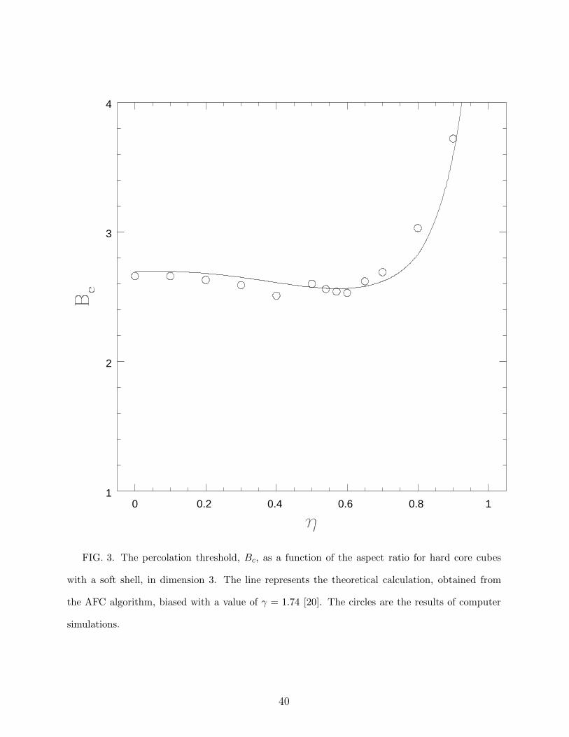
FIG. 3. The percolation threshold, Bc, as a function of the aspect ratio for hard core cubes

with a soft shell, in dimension 3. The line represents the theoretical calculation, obtained from

the AFC algorithm, biased with a value of γ = 1.74 [20]. The circles are the results of computer

simulations.

40

0 0.2 0.4 0.6 0.8 11

2

3

4

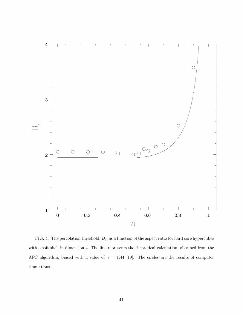
FIG. 4. The percolation threshold, Bc, as a function of the aspect ratio for hard core hypercubes

with a soft shell in dimension 4. The line represents the theoretical calculation, obtained from the

AFC algorithm, biased with a value of γ = 1.44 [19]. The circles are the results of computer

simulations.

41

0 0.2 0.4 0.6 0.8 10

1

2

3

4

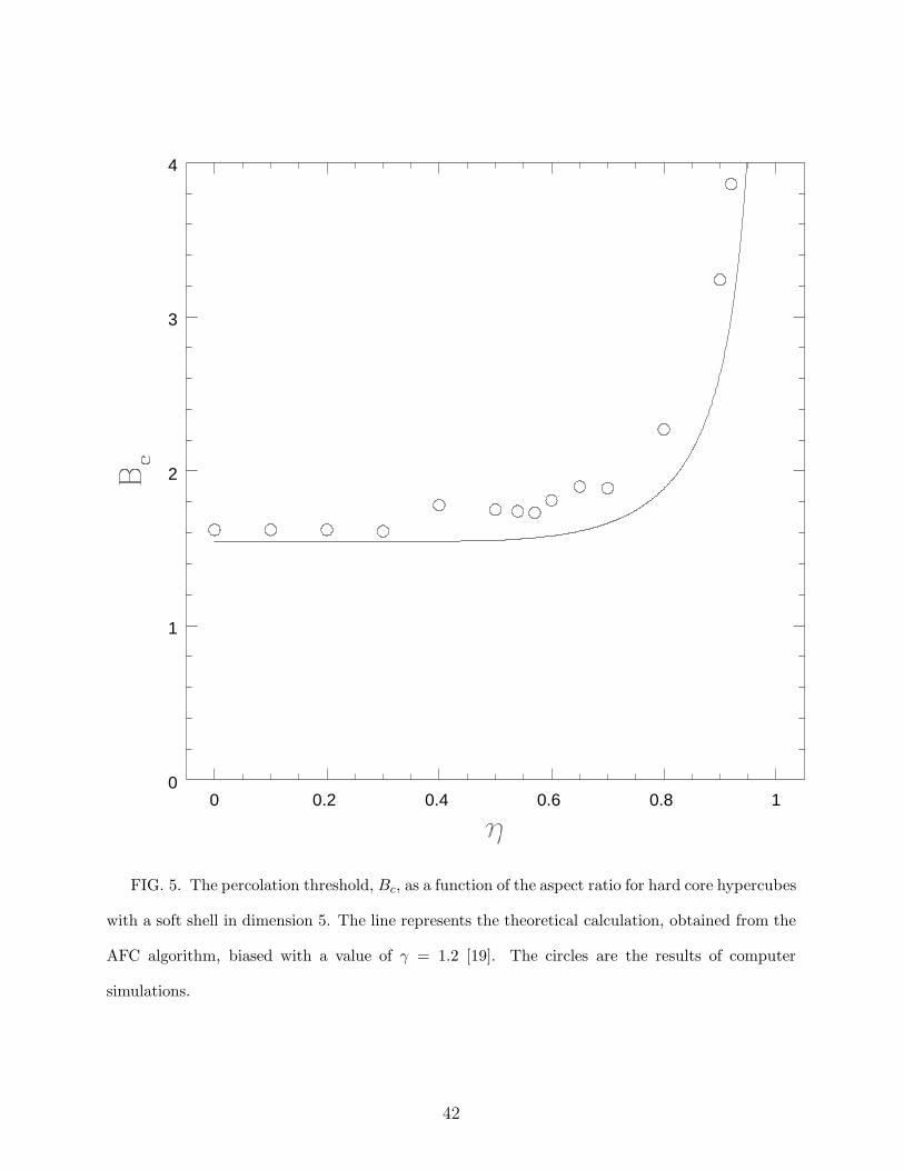
FIG. 5. The percolation threshold, Bc, as a function of the aspect ratio for hard core hypercubes

with a soft shell in dimension 5. The line represents the theoretical calculation, obtained from the

AFC algorithm, biased with a value of γ = 1.2 [19]. The circles are the results of computer

simulations.

42