Journal of Statistical Planning and Inference 138 (2008) 3647 -- 3659

Contents lists available at ScienceDirect

Journal of Statistical Planning and Inference

journal homepage: www.e lsev ier .com/ locate / j sp i

Lower bounds on expectations of positive L-statistics fromwithout-replacement models

Agnieszka Goroncya, Tomasz Rychlikb,∗aNicolaus Copernicus University, Chopina 12, 87100 Torun, PolandbInstitute of Mathematics, Polish Academy of Sciences, Nicolaus Copernicus University, Chopina 12, 87100 Torun, Poland

A R T I C L E I N F O A B S T R A C T

Article history:Received 21 July 2006Received in revised form8 August 2007Accepted 11 November 2007Available online 25 March 2008

MSC:primary 62G30secondary 60C0560E1562D05

Keywords:ExpectationOrder statisticL-StatisticDrawing without replacementFinite populationOptimal bound

We consider samples drawn without replacement from finite populations. We establishoptimal lower non-negative and upper non-positive bounds on the expectations of linearcombinations of order statistics centered about the populationmean in units generated by thepopulation central absolute moments of various orders. We also specify the generalresults for important examples of sample extremes, Gini mean differences and sample range.The paper completes the results of Papadatos and Rychlik [2004. Bounds on expectations ofL-statistics fromwithout replacement samples. J. Statist. Plann. Inference124, 317--336],wheresharp negative lower and positive upper bounds on the expectations of the combinationswerepresented for the without-replacement samples.

© 2008 Elsevier B.V. All rights reserved.

1. Introduction

Let � = {x1, . . . , xN } ⊂ R be a population of size N whose elements are not all identical, and let X = (X1, . . . , Xn) be a sampleof the size n taken from � without replacement. We assume 2�n�N, and the case n = N leads to the exhaustive drawing from�. We denote the ordered elements of the sample and population by X1:n � · · · �Xn:n and x1:N � · · · �xN:N , respectively. Theobservations are dependent identically distributed and the finite mean and central absolute moments are given by

� = EX1 = 1N

N∑i=1

xi,

�pp = E|X1 − �|p = 1

N

N∑i=1

|xi − �|p, 1�p < ∞. (1.1)

∗ Corresponding author.E-mail addresses: gemini@mat.uni.torun.pl (A. Goroncy), trychlik@impan.gov.pl (T. Rychlik).

0378-3758/$ - see front matter © 2008 Elsevier B.V. All rights reserved.doi:10.1016/j.jspi.2007.11.016

3648 A. Goroncy, T. Rychlik / Journal of Statistical Planning and Inference 138 (2008) 3647 -- 3659

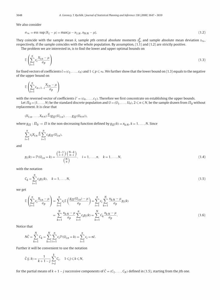
We also consider

�∞ = ess sup |X1 − �| = max{� − x1:N, xN:N − �}. (1.2)

They coincide with the sample mean x, sample pth central absolute moments spp, and sample absolute mean deviation s∞,

respectively, if the sample coincides with the whole population. By assumption, (1.1) and (1.2) are strictly positive.The problem we are interested in, is to find the lower and upper optimal bounds on

E

⎛⎝ n∑

i=1

ciXi:n − �

�p

⎞⎠ (1.3)

for fixed vectors of coefficients c=(c1, . . . , cn) and 1�p�∞.We further show that the lower bound on (1.3) equals to the negativeof the upper bound on

E

⎛⎝ n∑

i=1

cn+1−iXi:n − �

�p

⎞⎠

with the reversed vector of coefficients c′ = (cn, . . . , c1). Therefore we first concentrate on establishing the upper bounds.Let�0 ={1, . . . , N} be the standard discrete population and U = (U1, . . . , Un), 2�n�N, be the sample drawn from�0 without

replacement. It is clear that

(X1:n, . . . , Xn:n)d=(g�(U1:n), . . . , g�(Un:n)),

where g� : �0 → � is the non-decreasing function defined by g�(k) = xk:N , k = 1, . . . , N. Since

n∑i=1

ciXi:nd=

n∑i=1

cig�(Ui:n),

and

pi(k) = P(Ui:n = k) =(

k−1i−1

) (N−kn−i

)(

Nn

) , i = 1, . . . , n, k = 1, . . . , N, (1.4)

with the notation

Ck =n∑

i=1

cipi(k), k = 1, . . . , N, (1.5)

we get

E

⎛⎝ n∑

i=1

ciXi:n − �

�p

⎞⎠ =

n∑i=1

ciE

(g�(Ui:n) − �

�p

)=

n∑i=1

ci

N∑k=1

xk:N − ��p

pi(k)

=N∑

k=1

xk:N − ��p

n∑i=1

cipi(k) =N∑

k=1

Ckxk:N − �

�p. (1.6)

Notice that

NC =N∑

k=1

Ck =N∑

k=1

n∑i=1

ciP(Ui:n = k) =n∑

i=1

ci = nc.

Further it will be convenient to use the notation

C(j, k) = 1k + 1 − j

k∑i=j

Ci, 1� j�k�N,

for the partial means of k + 1 − j successive components of C = (C1, . . . , CN) defined in (1.5), starting from the jth one.

A. Goroncy, T. Rychlik / Journal of Statistical Planning and Inference 138 (2008) 3647 -- 3659 3649

Papadatos and Rychlik (2004) determined positive optimal bounds on expectations of arbitrary L-statistics under the followingcondition

minj=1,...,N−1

C(1, j) < C(1, N) = C. (1.7)

By (1.4) and (1.5), Eq. (1.7) represents implicit conditions on the original vector of coefficients c. The bounds were derived by useof the l2-projection C of C onto the convex cone of non-decreasing sequences in RN . The projection is determined by means ofthe following algorithm. First, we define the subset of indices {j1, . . . , jM} ⊂ {1, . . . , N} as follows

jm+1 = min{jm + 1� j�N : C(jm + 1, j) is minimal},with j0 = 0 and jM = N for some 1�M�N. Then we define the projection vector C as

Ck = C(jm−1 + 1, jm), k = jm−1 + 1, . . . , jm, m = 1, . . . , M. (1.8)

Applying the projection method, for 1< p < ∞ and 1< q = p/(p − 1) < ∞ we obtain

E

⎛⎝ n∑

i=1

ciXi:n − �

�p

⎞⎠ =

N∑i=1

Cixi:N − �

�p

�N∑

i=1

Cixi:N − �

�p=

N∑i=1

(Ci − cq)xi:N − �

�p

�⎛⎝ N∑

i=1

∣∣∣∣ xi − ��p

∣∣∣∣p⎞⎠1/p⎛

⎝ N∑i=1

|Ci − cq|q⎞⎠1/q

= N1/p‖C − cq1‖q, (1.9)

where cq is the unique solution to the equation

N∑i=1

|Ci − cq|q/psgn{Ci − cq} = 0,

and it minimizes the function c �→ ‖C − c1‖q, c ∈ R. The equality in (1.9) holds for the unique ordered population � ={x1:N � · · · �xN:N } with

xk:N − ��p

= N1/p|Ci − cq|q/psgn{Ci − cq}(∑N

i=1 |Ci − cq|q)1/p, k = 1, . . . , N. (1.10)

Condition (1.7) implies that sequence (1.8) is not constant, the bound in (1.9) is positive, and (1.10) have non-zero denominatorsand are well defined. Slightly modifying the arguments of (1.9), we get analogous bounds for the extreme values p = 1 and ∞.

Optimal positive upper bounds on L-statistics in the special case of exhaustive samples were presented in Rychlik (1992,1993). They covered special cases of particular L-statistics presented, among others, in Scott (1936), Nair (1948), Mallows andRichter (1969), Boyd (1971), Hawkins (1971), Beesack (1973), Fahmy and Proschan (1981), and David (1988). Balakrishnanet al. (2003) presented positive upper expectation bounds on single order statistics and sample range based on non-exhaustivesamples, expressed in terms of the standard deviation units �2. They also determined strictly positive lower standard deviationbounds on the samplemaxima and upper negative bounds on the sampleminima, generalizing the evaluations of Boyd (1971) andHawkins (1971) for exhaustive drawing. Goroncy and Rychlik (2006a) established general deterministic non-negative lower andnon-positive upper bounds on arbitrary L-statistics based on exhaustive samples, expressed in terms of various samplemoments.They are used in Section 2 for calculating respective generalizations to non-exhaustive drawing in without-replacement models.General results are specified for special cases of samples extremes, Gini mean differences and sample ranges in Section 3. Wealso mention that analogous positive and negative upper bounds for the with-replacement drawing schemes were described inRychlik (2004), and Goroncy and Rychlik (2006b), respectively. Sample maxima, ranges, and non-extreme order statistics wereevaluated by Lopez-Blazquez (1998, 2000) and Lopez-Blazquez and Rychlik (2008), respectively, for a more general model of i.i.d.sampling from finite populations with arbitrary marginal distribution.

2. General results

We provide the optimal upper non-positive bounds on the expectations of L-statistics in the case, when the projection C ofthe vector C onto the convex cone of non-decreasing vectors (cf. (1.5) and (1.8)) is a constant, and the projection method resultswith the zero bounds. We show that this zero bound can be improved for some c.

3650 A. Goroncy, T. Rychlik / Journal of Statistical Planning and Inference 138 (2008) 3647 -- 3659

Theorem 1. Let 1�p < ∞ and c ∈ Rn be a vector satisfying

minj=1,...,N−1

C(1, j)� C (2.1)

(cf. (1.7)). Put

Lp,c(j) =[

Np+1

jp(N − j) + j(N − j)p

]1/p

j [C(1, j) − C], j = 1, . . . , N − 1. (2.2)

Then

E

⎛⎝ n∑

i=1

ciXi:n − �

�p

⎞⎠ � − min

j=1,...,N−1Lp,c(j), (2.3)

with the equality attained for the following ordered population

x(j,p)k:N =

⎧⎪⎪⎪⎪⎨⎪⎪⎪⎪⎩

� − �p(N − j)

[Np+1

j(N − j)p + jp(N − j)

]1/p

, k = 1, . . . , j,

� + �pj

[Np+1

j(N − j)p + jp(N − j)

]1/p

, k = j + 1, . . . , N,

(2.4)

with j = j∗ where j∗ minimizes (2.2).

Proof. This is an immediate consequence of Goroncy and Rychlik (2006a, Theorem 1). By (1.6), we have

E

⎛⎝ n∑

i=1

ciXi:n − �

�p

⎞⎠ =

N∑k=1

Ckxk:N − �

�p=

N∑k=1

(Ck − C)xk:N − �

�p,

where � and �pp coincide with the sample mean x and pth absolute central moment s

pp of the deterministic sample {x1, . . . , xN }.

Goroncy and Rychlik (2006a) proved that under condition (2.1) the following deterministic bounds hold:

N∑k=1

(Ck − C)xk:N − x

sp� − min

j=1,...,N−1

[Np+1

jp(N − j) + j(N − j)p

]1/p

j[C(1, j) − C]

= − minj=1,...,N−1

Lp,c(j).

On the other hand, we easily verify that for the populations (2.4) we have

E

⎛⎝ n∑

i=1

ciXi:n − �

�p

⎞⎠ = −Lp,c(j), j = 1, . . . , N − 1,

which ends the proof. �

Applying the results of Goroncy and Rychlik (2006a, Theorem 2) we can also prove analogous evaluations for p = ∞.

Theorem 2. Let c ∈ Rn be a vector satisfying (2.1). Put

L∞,c (j) = N

max{j, N − j} j[C(1, j) − C], j = 1, . . . , N − 1. (2.5)

Then

E

⎛⎝ n∑

i=1

ciXi:n − �

�∞

⎞⎠ � − min

j=1,...,N−1L∞,c (j), (2.6)

A. Goroncy, T. Rychlik / Journal of Statistical Planning and Inference 138 (2008) 3647 -- 3659 3651

with the equality attained for the ordered population

x(j,∞)k:N =

{� − �∞, k = 1, . . . , j,

� + �∞j

N − j, k = j + 1, . . . , N,

if 1� j� N

2, (2.7)

x(j,∞)k:N =

{� − �∞

N − j

j, k = 1, . . . , j,

� + �∞, k = j + 1, . . . , N,if

N

2� j�N − 1, (2.8)

with j = j∗ where j∗ minimizes (2.5).

The above two theorems allow us to calculate optimal upper inequalities for arbitrary L-statistics with non-positive expec-tations in arbitrary scale units determined by central absolute population moments. It merely suffices to compare numericallyN − 1 values of functions (2.2) and (2.5).

Below we present an application of Theorems 1 and 2 for establishing sharp lower bounds for L-statistics with non-negativeexpectations.

Corollary 1. Let c ∈ Rn satisfy

maxj=1,...,N−1

C(1, j)� C (2.9)

(cf. (2.1)), and set c′ = (cn, . . . , c1). Then for every 1�p�∞, we have

E

⎛⎝ n∑

i=1

ciXi:n − �

�p

⎞⎠ � min

j=1,...,N−1Lp,c′ (j)

(cf. (2.3) and (2.6)), and the equality is attained for the ordered population x(N−j′∗,p)k:N , k = 1, . . . , N, (cf. (2.4), (2.7) and (2.8)) where j′∗

minimizes Lp,c′ (j), j = 1, . . . , N − 1.

Proof. Let X1, . . . , Xn be a sample drawn without replacement from a population � = {x1, . . . , xN } with mean � and �p >0. Takeanother population�′ = {x′

1, . . . , x′N } with x′

k=2�− xk , k =1, . . . , N, and draw X ′

1, . . . , X ′n without replacement from�′. Note that

X ′i, i = 1, . . . , n, have the same mean � and dispersion parameters �p, 1�p�∞, and x′

k:N = 2� − xN+1−k:N , k = 1, . . . , N. Since

pi(k) = pn+1−i(N + 1 − k), i = 1, . . . , n, k = 1, . . . , N,

we have

E

⎛⎝ n∑

i=1

c′i

X ′i:n − ��p

⎞⎠ =

n∑i=1

c′i

N∑k=1

x′k:N − �

�ppi(k)

=N∑

k=1

� − xN+1−k:N�p

n∑i=1

cn+1−i pn+1−i(N + 1 − k)

= −N∑

k=1

CN+1−kxN+1−k:N − �

�p= −E

⎛⎝ n∑

i=1

ciXi:n − �

�p

⎞⎠ .

Therefore

inf E

⎛⎝ n∑

i=1

c′i

X ′i:n − ��p

⎞⎠ = − supE

⎛⎝ n∑

i=1

ciXi:n − �

�p

⎞⎠ = min

j=1,...,N−1Lp,c′ (j), (2.10)

where the infimum and supremum are taken over arbitrary numerical populations of size N with �p >0. The infimum isnon-negative if condition

minj=1,...,N−1

C ′(1, j) = minj=1,...,N−1

1j

j∑k=1

C ′k� C ′ = 1

N

N∑k=1

C ′k

(2.11)

holds with

C ′k

=n∑

i=1

c′ipi(k) =

n∑i=1

cn+1−ipn+1−i(N + 1 − k) = CN+1−k, k = 1, . . . , N.

3652 A. Goroncy, T. Rychlik / Journal of Statistical Planning and Inference 138 (2008) 3647 -- 3659

It is easy to verify that (2.11) is identical with (2.9). If the supremum of (2.10) is attained by some ordered two-valued population

x(j′∗,p)k:N , k = 1, . . . , N, (see (2.4), (2.7) and (2.8)), then the infimum is attained by x

(j∗,p)k:N = 2� − x

(j′∗,p)N+1−k:N = x

(N−j′∗,p)k:N , k = 1, . . . , N.

This completes the proof. �

Suppose that c satisfying the assumption of Corollary 1 has the property

cn+1−i − c = c − ci, i = 1, . . . , n.

Then

CN+1−k − C =n∑

i=1

cipi(N + 1 − k) − C =n∑

i=1

(2c − cn+1−i)pn+1−i(k) − C

= 2cn∑

i=1

P(Ui = k) − Ck − C = C − Ck, k = 1, . . . , N.

Clearly, the primed sequences c′ and C ′ have analogous properties. It follows that

j[C ′(1, j) − C ′] =j∑

k=1

(C ′k

− C ′) =j∑

k=1

(C ′ − C ′N+1−k

)

= j

N

N∑k=1

C ′k

−N∑

k=N+1−j

C ′k

=N−j∑k=1

C ′k

− N − j

N

N∑k=1

C ′k

= (N − j)[C ′(1, N − j) − C ′], j = 1, . . . , N − 1.

Since the former factors in (2.2) and (2.5) are symmetric about N/2 as well, so are all the functions Lp,c′ , 1�p�∞. If they areminimized at some j′∗, the sameholds forN−j′∗. Owing to the latter statement of Corollary 1, the two-valued populations providingthe minimal expectations of respective L-statistics have j′∗ and N − j′∗ identical elements. Below we describe optimal inequalitiesfor some L-statistics which are of special interest.

3. Examples

In order to find the optimal bounds on expectations of specific L-statistics, we need to analyze

Lc,p(j) = Ac(j)Bp(j), 1� j�N − 1, (3.1)

where

Ac(j) = j [C(1, j) − C] =j∑

k=1

(Ck − C), (3.2)

with C = (C1, . . . , CN) defined in (1.5), dependent on the coefficients c1, . . . , cn, and

Bp(j) =

⎧⎪⎪⎪⎨⎪⎪⎪⎩

[N1+p

jp(N − j) + j(N − j)p

]1/p

, 1�p < ∞,

N

max{j, N − j} , p = ∞,

(3.3)

depending only on the range p of the scale unit �p and being the same for various L-statistics. For specific types of L-statistics,(3.2) depends on n, N and j.

3.1. Sample minimum X1:n

The coefficient vector c = (1,0, . . . ,0) has the mean c = 1/n. Therefore

Ci = P(U1:n = i) =(

N−in−1

)(

Nn

) , i = 1, . . . , N,

A. Goroncy, T. Rychlik / Journal of Statistical Planning and Inference 138 (2008) 3647 -- 3659 3653

and C = 1/N. We have

Ac(j) =j∑

i=1

(Ci − C) =j∑

i=1

P(U1:n = i) − j

N= 1 − P(U1:n > j) − j

N

= N − j

N−

(N−jn

)(

Nn

) = N − j

N− (N − j)(N − j − 1) · · · (N − j − n + 1)

N(N − 1) · · · (N − n + 1)

= Amn (j), (3.4)

say. The equality between the first and second lines follows from the fact that the event {U1:n > j} is equivalent to drawing nnumbers from the subset {j + 1, . . . , N}.

Proposition 1. We have

E

(X1:n − �

�p

)� −

⎧⎪⎪⎨⎪⎪⎩

[N

(N − 1) + (N − 1)p

]1/p

, 1�p < ∞,

1N − 1

, p = ∞,

(3.5)

If 1�p < ∞ (p = ∞, respectively), then the equality in (3.5) holds for (2.4) ((2.8), respectively) with j = N − 1. Moreover, if n = 2 and1< p < ∞ (p = ∞, respectively), then the equality holds for (2.4) ((2.7), respectively) with j = 1 as well. In the case n = 2 and p = 1,the equality is attained by (2.4) with arbitrary j = 1, . . . , N − 1.

Proof. We aim at analyzing (3.1) with (3.2) specified in (3.4), and (3.3). Put first n = 2. Then

Am2 (j) = j(N − j)

N(N − 1).

Under the notation

Lmp,n(j) = Am

n (j)Bp(j),

we have

Lmp,2(j) =

⎧⎪⎪⎪⎪⎪⎪⎪⎨⎪⎪⎪⎪⎪⎪⎪⎩

N

N − 1·

j

N

(1 − j

N

)[

j

N

(1 − j

N

)p

+(

j

N

)p (1 − j

N

)]1/p, 1�p < ∞,

min{j, N − j}N − 1

, p = ∞.

(3.6)

If p = 1, then

Lm1,2(j) = N

2(N − 1)

is a constant and so is minimized by every j = 1, . . . , N − 1. Let 1< p < ∞. We have

Lmp,2(j) = N

N − 1· 1[

Vp

(j

N

)]1/p, 1� j�N − 1,

where

Vp(x) = x1−p + (1 − x)1−p, 0< x <1.

is a function symmetric about 12 that is first decreasing and then increasing. Therefore

min1� j�N−1

Lmp,2(j) = Lm

p,2(1) = Lmp,2(N − 1) =

[N

(N − 1) + (N − 1)p

]1/p

. (3.7)

3654 A. Goroncy, T. Rychlik / Journal of Statistical Planning and Inference 138 (2008) 3647 -- 3659

From (3.6) we also easily conclude that

min1� j�N−1

Lm∞,2(j) = Lm

∞,2(1) = Lm∞,2(N − 1) = 1

N − 1.

Consider n >2 now. Note that for fixed j and increasing n, (3.4) is first increasing for 2�n�N +1− j, and ultimately a constantfor N + 1 − j�n�N with the maximal value (N − j)/N. Accordingly, we have

Amn (j)�Am

2 (j), 1� j�N − 1, 2�n�N. (3.8)

In particular, Amn (1) is strictly increasing, and Am

n (N − 1) = 1/N is a constant for 2�n�N. This implies

Lmp,n(j)�Lm

p,2(j)�Lmp,2(N − 1) = Lm

p,n(N − 1) (3.9)

for arbitrary 1�p�∞, 2�n�N and 1� j�N − 1. We get the first inequality once we multiply (3.8) by a positive term (3.3),independent of n. The other was established above. The equality follows from the fact that both the factors in Lm

p,n(N − 1) areindependent of n. The last expression amounts to (3.5).

It suffices to show that at least one inequality in (3.9) is strict for j�N − 1 and n�3. If p >1, then Lmp,2(j) > Lm

p,2(N − 1) for

j = 2, . . . , N − 2, and Amn (1) > Am

2 (1) implies

Lmp,n(1) > Lm

p,2(1) = Lmp,2(N − 1) = Lm

p,n(N − 1).

If p = 1, the relation Lm1,n

(j) = Lm1,n−1(j) for some j�N − 2, yields Am

n (j) = (N − j)/N, and so

Lm1,n(j) = N

2j> Lm

1,n(N − 1) = N

2(N − 1).

This ends the proof. �

Bounds (3.5) are independent of the sample size n. As the population size N increases, they tend to 0 except for the case p = 1,with the limiting value 1

2 . For p = 1 and 2 we obtain simple forms

E

(X1:n − �

�p

)� −

⎧⎪⎨⎪⎩

N

2(N − 1), p = 1,

1√N − 1

, p = 2.

Particular inequalities for p=2 and n=N were presented by Boyd (1971) andHawkins (1971). The case p=2with n < N was solvedbyBalakrishnanet al. (2003). Goroncy andRychlik (2006b) showed that respective evaluations for the sampling-with-replacementscheme are 1 − 1/Nn−1 times smaller, and are attained by the same populations.

By Corollary 1, the lower bounds on the expectation of the sample maximum Xn:n equal the negatives of the upper boundsfor the minimum X1:n, presented in Proposition 1. They are attained if one element of the population is less than all the otheridentical ones. If n=2 in particular, it suffices to assume that the population has exactly N −1 identical elements. When n=2 andp = 1, the lower bounds are attained by arbitrary two-valued populations. The coefficients of L-statistics treated in Sections 3.2and 3.3 are antisymmetric about (n+1)/2. Due to the considerations of the last part of Section 2, the solutions of theminimizationproblems directly describe the optimal partitions of two-valued populations.

3.2. Gini mean differences

Let

Gn = 1n(n − 1)

n∑i,j=1

|Xi − Xj| = 2n(n − 1)

n∑i=1

(2i − n − 1)Xi:n. (3.10)

In order to find the lower bound on the expectations of (3.10), we use the reversed coefficient vector of the L-statistics, which hasthe components

c′i = cn+1−i = 2(n + 1 − 2i)

n(n − 1)= −ci, i = 1, . . . , n.

A. Goroncy, T. Rychlik / Journal of Statistical Planning and Inference 138 (2008) 3647 -- 3659 3655

This immediately implies that c′ = 0, and in consequence C = 0. Next, we determine

Ci =n∑

r=1

c′rP(Ur:n = i) =

n∑r=1

2(n + 1 − 2r)

n(n − 1)·(

i−1r−1

) (N−in−r

)(

Nn

)

=n−1∑s=0

2(n − 1 − 2s)

n(n − 1)·(

i−1s

) (N−i

n−1−s

)(

Nn

)

=n−1∑s=0

2(n − 1 − 2s)

N(n − 1)·(

i−1s

) (N−i

n−1−s

)(

N−1n−1

) , i = 1, . . . , N.

Note that these are the expectations of linear functions 2(n − 1 − 2Si)/N(n − 1) of random variables Si with the hypergeometricdistributions HG(N − 1, i − 1, n − 1), i = 1, . . . , N. Here Si represents the number of white balls in a sample of size n − 1 drawnwithout replacement from an urn with i − 1 white and N − i black balls. Therefore

Ci = E

(2(n − 1 − 2Si)

N(n − 1)

)= 2(N + 1 − 2i)

N(N − 1), i = 1, . . . , N,

and so

Ac(j) =j∑

i=1

Ci = 2j(N − j)

N(N − 1)= Ag(j),

Lc,p(j) = Lgp(j) = Ag(j)Bp(j), j = 1, . . . , N − 1, (3.11)

which do not depend on n. We can note that functions (3.11) we minimize are identical with those of the deterministic modelwith n = N considered in Goroncy and Rychlik (2006a, Example 3). Therefore we immediately obtain the followingresults.

Proposition 2. (i) If 1�p < ∞, then

E

(Gn

�p

)�2

[N

(N − 1) + (N − 1)p

]1/p

,

and the equality holds for (2.4) with j = 1 and with j = N − 1 for p >1, and with arbitrary j = 1, . . . , N − 1 for p = 1.(ii) If p = ∞, then

E

(Gn

�p

)�L∞(1) = L∞(N − 1) = 2

N − 1,

and the equality holds for (2.7) with j = 1 and for (2.8) with j = N − 1.

We also observe that the bounds of the Proposition 2 are N/(N − 1) times greater than the respective bounds in the drawing-with-replacement model, presented in Goroncy and Rychlik (2006b, Proposition 2), and twice as much as those for the samplemaxima, determined in Proposition 1.

3.3. Sample range Xn:n − X1:n

The coefficient vector of the L-statistic is c = (−1,0, . . . ,0,1). In order to find the lower positive bound, we use the reversedcoefficient vector c′ = (1,0, . . . ,0, −1). Obviously c′ = 0 which implies C = 0, whereas

Ci = P(U1:n = i) − P(Un:n = i) =(

N−in−1

)(

Nn

) −(

i−1n−1

)(

Nn

) , i = 1, . . . , N. (3.12)

Accordingly,

Ac(j) =j∑

i=1

Ci = 1 − P(U1:n > j) − P(Un:n � j)

= 1(Nn

) [(N

n

)−

(N − j

n

)−

(j

n

)]= Ar

n(j), (3.13)

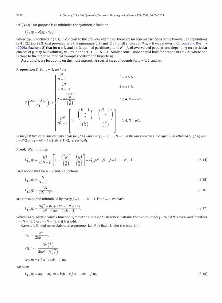
3656 A. Goroncy, T. Rychlik / Journal of Statistical Planning and Inference 138 (2008) 3647 -- 3659

(cf. (3.4)). Our purpose is to minimize the symmetric function

Lrp,n(j) = Ar

n(j) · Bp(j),

where Bp(j) is defined in (3.3). In contrast to the previous examples, there are no general partitions of the two-values populations(2.4), (2.7), or (2.8) that provides here the minimum (2.3) and (2.6) for all choices of N, n, p. It was shown in Goroncy and Rychlik(2006a, Example 2) that for n = N and p >3, optimal partitions j∗ and N − j∗ of two-valued populations, depending on particularchoices of p, may take arbitrary values in the set {1, . . . , N − 1}. Similar conclusions should hold for other pairs n < N, where oneis close to the other. Numerical examples confirm the hypothesis.

Accordingly, we focus only on the most interesting special cases of bounds for p = 1, 2, and ∞.

Proposition 3. For p = 1, we have

E

(Xn:n − X1:n

�1

)�

⎧⎪⎪⎪⎪⎪⎪⎪⎪⎪⎪⎪⎪⎪⎪⎪⎪⎪⎪⎪⎪⎪⎪⎪⎨⎪⎪⎪⎪⎪⎪⎪⎪⎪⎪⎪⎪⎪⎪⎪⎪⎪⎪⎪⎪⎪⎪⎪⎩

N

N − 1, 2 = n�N,

3N

2(N − 1), 3 = n�N,

2 − 4

(N/2n

)(

Nn

) , n�4, N − even,

2N2

N2 − 1

⎡⎢⎢⎢⎢⎢⎢⎣1 −

⎛⎝ N − 1

2n

⎞⎠

(Nn

) −

⎛⎝ N + 1

2n

⎞⎠

(Nn

)

⎤⎥⎥⎥⎥⎥⎥⎦

n�4, N − odd.

In the first two cases, the equality holds for (2.4)with every j = 1, . . . , N − 1. In the last two cases, the equality is attained by (2.4)withj = N/2 and j = (N − 1)/2, (N + 1)/2, respectively.

Proof. Weminimize

Lr1,n(j) = N2

2j(N − j)

⎡⎣1 −

(N−jn

)(

Nn

) −(

jn

)(

Nn

)⎤⎦ = Lr

1,n(N − j), j = 1, . . . , N − 1. (3.14)

First notice that for n = 2 and 3, functions

Lr1,2(j) = N

N − 1, (3.15)

Lr1,3(j) = 3N

2(N − 1), (3.16)

are constant and minimized by every j = 1, . . . , N − 1. For n = 4, we have

Lr1,4(j) = N(j2 − jN + 2N2 − 9N + 11)

(N − 1)(N − 2)(N − 3), (3.17)

which is a quadratic convex function symmetric aboutN/2. Therefore it attains theminimum for j=N/2 ifN is even, and for eitherj = (N − 1)/2 or j = (N + 1)/2, if N is odd.

Cases n�5 need more elaborate arguments. Let N be fixed. Under the notation

b(j) = N2

2j(N − j),

c(j, n) =N2

(jn

)2j(N − j)

(Nn

) ,a(j, n) = c(j, n) + c(N − j, n),

we have

Lr1,n(j) = b(j) − a(j, n) = b(j) − c(j, n) − c(N − j, n). (3.18)

A. Goroncy, T. Rychlik / Journal of Statistical Planning and Inference 138 (2008) 3647 -- 3659 3657

We consider the increments of the difference sequence a(j, n) − a(j + 1, n), when n increases

�(j, n) = [a(j, n) − a(j + 1, n)] − [a(j, n + 1) − a(j + 1, n + 1)]= c(j, n) + c(N − j, n) − c(j + 1, n) − c(N − j − 1, n) − c(j, n + 1)

− c(N − j, n + 1) + c(j + 1, n + 1) + c(N − j − 1, n + 1).

Observing that

c(j, n + 1) = j − n

N − nc(j, n),

c(N − j, n + 1) = N − j − n

N − nc(N − j, n),

c(j + 1, n + 1) = j − n + 1N − n

c(j + 1, n),

c(N − j − 1, n + 1) = N − j − n − 1N − n

c(N − j − 1, n),

and writing ck = c(k, n) for brevity, we obtain

�(j, n) = 1N − n

[(N − j)cj + j cN−j − (N − j − 1)cj+1 − (j + 1)cN−j−1].

Since

cj+1 = j(N − j)

(N − j − 1)(j − n + 1)cj ,

cN−j−1 = j(N − j − n)

(j + 1)(N − j − 1)cN−j

we finally obtain

�(j, n) = 1N − n

[− (n − 1)(N − j)

j − n + 1cj + j(n − 1)

N − j − 1cN−j

]

= N(n − 1)

2(N − 1) · · · (N − n)

× [(N − j − 2) · · · (N − j − n + 1) − (j − 1) · · · (j − n + 2)].

The fraction in front of the brackets is positive. The expression in the brackets is the difference of two products of consecutiven − 2 integers arranged in the decreasing order. This is positive iff N − j − 2> j − 1 and N − j − n + 1>0, i.e. for j < (N − 1)/2 andj�N − n. Likewise, this is negative iff j > (N − 1)/2 and j�n − 1, and amounts to zero in all the remaining cases. Accordingly,we can write

�(j, n)�0, j <N − 12

,

and, equivalently,

a(j, n) − a(j + 1, n)�a(j, n + 1) − a(j + 1, n + 1), j <N − 12

. (3.19)

Note that the differences

b(j) − b(j + 1) = N2(N − 2j + 1)

2j(N − j)(j + 1)(N − j − 1)

are independent of n and are positive iff j < (N − 1)/2.Now we are in a position to prove

Lr1,n(j) > Lr

1,n(j + 1), j <N − 12

, (3.20)

for all 4�n�N. We apply the induction argument with respect to n. Using (3.17), we proved that the statement holds true forn = 4. Assume the same for some n�4. By (3.18), it is equivalent to the claim

b(j) − b(j + 1) > a(j, n) − a(j + 1, n), j <N − 12

.

3658 A. Goroncy, T. Rychlik / Journal of Statistical Planning and Inference 138 (2008) 3647 -- 3659

This combined with (3.19) yield

b(j) − b(j + 1) > a(j, n + 1) − a(j + 1, n + 1),

which coincides with

Lr1,n+1(j) > Lr

1,n+1(j + 1), j <N − 12

,

and establishes (3.20) for all n�4. This claim, together with symmetry of (3.14) with respect to N/2, completes the proof of thefact that (3.14) is minimized either by j =N/2 or j = (N −1)/2 and (N +1)/2 in the cases of N being even and odd, respectively. �

Notice that forn > N/2with evenN, and forn > (N+1)/2withN odd, the third and fourth bounds simplify to 2 and2N2/(N2−1),respectively. They are attained by populations with two values, and the numbers of both types of elements are either equal oralmost equal. The respective bounds in the maximal absolute mean deviation units �∞ are attained by the populations withonly one element different from the others. The same populations have minimal expectations of ranges for the drawing-with-replacement models.

Proposition 4. For p = ∞,

E

(Xn:n − X1:n

�∞

)� n

N − 1,

and the equality holds for (2.7) when j = 1 and for (2.8) when j = N − 1.

Proof. We analyze

Lr∞,n(j) = Arn(j)B∞(j) = Ar

n(j)N

max{j, N − j} , j = 1, . . . , N − 1,

where Arn(j) is defined in (3.13). It is easy to see that sequence (3.12) is non-increasing, and so

2Arn(j) = 2

j∑i=1

Ci �j−1∑i=1

Ci +j+1∑i=1

Ci = Arn(j − 1) + Ar

n(j + 1), 2� j�N − 2,

which implies that Arn(j)� min{Ar

n(j − 1), Arn(j + 1)}. Therefore

min1� j�N−1

Arn(j) = min{Ar

n(1), Arn(N − 1)} = Ar

n(1) = Arn(N − 1) >0,

by symmetry. Also,

min1� j�N−1

B∞(j) = B∞(1) = B∞(N − 1) < min2� j�N−2

B∞(j). (3.21)

Therefore

min1� j�N−1

Arn(j)B∞(j)� min

1� j�N−1Ar

n(j) min1� j�N−1

B∞(j)

= Arn(1)B∞(1) = Ar

n(N − 1)B∞(N − 1) = n

N − 1.

By (3.21), these are the unique minimum points. �

Finally we discuss the case p = 2. We have

E

(Xn:n − X1:n

�2

)� min

1� j�N−1Lr2,n(j),

where

Lr2,n(j) = N√

j(N − j)(

Nn

) [(N

n

)−

(j

n

)−

(N − j

n

)]. (3.22)

Numerical evaluations for various n and N show that (3.22) is minimized by j = 1, N − 1 if n is small, and by j = N/2 (or j =(N ± 1)/2 for odd-sized populations) if n is large, and there are no other cases. The same statement was proved by Goroncy and

A. Goroncy, T. Rychlik / Journal of Statistical Planning and Inference 138 (2008) 3647 -- 3659 3659

Rychlik (2006b, Proposition 6) for the sampling-with-replacement model. The formal proof in the without-replacement case isan open problem. The trouble is that (3.22) is the product of two expressions of different types: analytic and combinatorial ones.When replacing is allowed, the combinatorial part is replaced by a polynomial of degree n in variable j/N, which makes theanalysis easier. Our conjecture for the without-replacement scheme can be supported by partial results. For instance, using

Lr2,n(j) = 2

√j(N − j)

NLr1,n(j),

we have

E

(X2:2 − X1:2

�2

)� min

1� j�N−12

√j(N − j)

N

N

N − 1= 2√

N − 1,

E

(X3:3 − X1:3

�2

)� min

1� j�N−12

√j(N − j)

N

3N

2(N − 1)= 3√

N − 1.

(cf. (3.15) and (3.16)). The first inequality was derived by Balakrishnan et al. (2003). Likewise, we show

E

(X2:2 − X1:2

�p

)�2

[N

(N − 1)p + N − 1

]1/p

,

E

(Xn:n − X1:n

�p

)�3

[N

(N − 1)p + N − 1

]1/p

,

for arbitraryp >1. Theseboundsare attainedby thepopulationswhereonlyoneelementdiffers fromtheothers. For theexhaustivedrawing, Goroncy and Rychlik (2006a) proved that

E

(XN:N − X1:N

�p

)�

⎧⎨⎩2, N − even,[

(2N)p+1

(N2 − 1)[(N − 1)p−1 + (N + 1)p−1]

]1/p

, N − odd.

If the population size N is even, then the minimal expectations are attained by two-valued populations with equal numbers ofidentical elements. For the odd-sized populations, the bound is attained when the numbers of identical elements differ by one.In the special case p = 2, the result is due to Thomson (1955).

Acknowledgements

The authors are grateful to an anonymous referee for helpful comments, especially for suggesting someprobabilistic argumentsthat simplified algebraic calculations in the original version of Section 3. The first and second authorswere supported by the PolishMinistry of Science and Higher Education Grant nos. N201 044 31/3695 and 1 P03A 015 30, respectively.

References

Balakrishnan, N., Charalambides, C., Papadatos, N., 2003. Bounds on expectation of order statistics from a finite population. J. Statist. Plann. Inference 113,569--588.

Beesack, P.R., 1973. On bounds for the range of ordered variates. Publ. Electrotechnical Faculty of Belgrade University Math. Phys. Ser. 428, 93--96.Boyd, A.V., 1971. Bound for ordered statistics. Publ. Electrotechnical Faculty of Belgrade University Math. Phys. Series 365, 31--32.David, H.A., 1988. General bounds and inequalities in order statistics. Commun. Statist.---Theor. Methods 17, 2119--2134.Fahmy, S., Proschan, F., 1981. Bounds on differences of order statistics. Amer. Statist. 35, 46--47.Goroncy, A., Rychlik, T., 2006a. How deviant can you be? The complete solution. Math. Inequal. Appl. 9, 633--647.Goroncy, A., Rychlik, T., 2006b. Lower bounds on expectations of positive L-statistics based on samples drawn with replacement. Statistics 40, 389--408.Hawkins, D.M., 1971. On the bounds of the range of ordered statistics. J. Amer. Statist. Assoc. 66, 644--645.Lopez-Blazquez, F., 1998. Discrete distributions with maximum expected value of the maximum. J. Statist. Plann. Inference 70, 201--207.Lopez-Blazquez, F., 2000. Bounds for the expected value of spacings from discrete distributions. J. Statist. Plann. Inference 84, 1--9.Lopez-Blazquez, F., Rychlik, T., 2008. Sharp upper bounds for the expected values of non-extreme order statistics from discrete distributions. J. Statist. Plann.

Inference, in press, doi:10.1016/j.jspi.2007.11.017.Mallows, C.L., Richter, D., 1969. Inequalities of Chebyshev type involving conditional expectations. Ann. Math. Statist. 40, 1922--1932.Nair, K.R., 1948. The distribution of the extreme deviate from the sample mean and its studentized form. Biometrika 35, 118--144.Papadatos, N., Rychlik, T., 2004. Bounds on expectations of L-statistics from without replacement samples. J. Statist. Plann. Inference 124, 317--336.Rychlik, T., 1992. Sharp inequalities for linear combinations of elements of monotone sequences. Bull. Polish Acad. Sci. Math. 40, 247--254.Rychlik, T., 1993. Sharp bounds on L-estimates and their expectations for dependent samples. Commun. Statist---Theor. Meth. 22, 1053--1068.Rychlik, T., 2004. Optimal bounds on L-statistics based on samples drawn with replacement from finite populations. Statistics 38, 391--412.Scott, J.M.C., 1936. Appendix to paper by Pearson and Chandra Sekar. Biometrika 28, 319--320.Thomson, G.W., 1955. Bounds on the ratio of range to standard deviation. Biometrika 42, 268--269.