Quantitative evaluation of automated skull-stripping methods applied to contemporary and legacy...

Quantitative Evaluation of Automated Skull-Stripping MethodsApplied to Contemporary and Legacy Images: Effects ofDiagnosis, Bias Correction, and Slice Location

Christine Fennema-Notestine1,2, I. Burak Ozyurt1,2, Camellia P. Clark1,2, ShaunnaMorris1,2, Amanda Bischoff-Grethe1,2, Mark W. Bondi1,2, Terry L. Jernigan1,2, BruceFischl3,4,5, Florent Segonne4,5, David W. Shattuck6,7, Richard M. Leahy6, David E. Rex7,Arthur W. Toga7, Kelly H. Zou8,9, Morphometry BIRN10, and Gregory G. Brown1,2,*

1 Laboratory of Cognitive Imaging, Department of Psychiatry, University of California, San Diego, La Jolla,California

2 Veterans Affairs San Diego Healthcare System, San Diego, California

3 Department of Radiology, Harvard Medical School, Charlestown, Massachusetts

4 Computer Science and Artificial Intelligence Laboratory, Massachusetts Institute of Technology,Cambridge, Massachusetts

5 Athinoula A. Martinos Center, MGH/NMR Center, Charlestown, Massachusetts

6 Signal and Image Processing Institute, and Depts. of Radiology and Biomedical Engineering, Universityof Southern California, Los Angeles, California

7 Laboratory of Neuro Imaging, Dept. of Neurology, University of California, Los Angeles, Los Angeles,California

8 Department of Radiology, Brigham and Women’s Hospital, Boston, Massachusetts

9 Department of Health Care Policy, Harvard Medical School, Cambridge, Massachusetts

10 Biomedical Informatics Research Network, www.nbirn.net

AbstractPerformance of automated methods to isolate brain from nonbrain tissues in magnetic resonance(MR) structural images may be influenced by MR signal inhomogeneities, type of MR image set,regional anatomy, and age and diagnosis of subjects studied. The present study compared theperformance of four methods: Brain Extraction Tool (BET; Smith [2002]: Hum Brain Mapp 17:143–155); 3dIntracranial (Ward [1999] Milwaukee: Biophysics Research Institute, Medical College ofWisconsin; in AFNI); a Hybrid Watershed algorithm (HWA, Segonne et al. [2004] Neuroimage22:1060–1075; in FreeSurfer); and Brain Surface Extractor (BSE, Sandor and Leahy [1997] IEEETrans Med Imag 16:41–54; Shattuck et al. [2001] Neuroimage 13:856 – 876) to manually strippedimages. The methods were applied to uncorrected and bias-corrected datasets; Legacy andContemporary T1-weighted image sets; and four diagnostic groups (depressed, Alzheimer’s, youngand elderly control). To provide a criterion for outcome assessment, two experts manually strippedsix sagittal sections for each dataset in locations where brain and nonbrain tissue are difficult todistinguish. Methods were compared on Jaccard similarity coefficients, Hausdorff distances, and anExpectation-Maximization algorithm. Methods tended to perform better on contemporary datasets;bias correction did not significantly improve method performance. Mesial sections were most

*Correspondence to: Dr. Gregory G. Brown, Laboratory of Cognitive Imaging (9151-B), 9500 Gilman Drive, MC 9151-B, Universityof California, San Diego, La Jolla, CA 92093. E-mail: [email protected].

NIH Public AccessAuthor ManuscriptHum Brain Mapp. Author manuscript; available in PMC 2008 June 2.

Published in final edited form as:Hum Brain Mapp. 2006 February ; 27(2): 99–113.

NIH

-PA Author Manuscript

NIH


NIH


difficult for all methods. Although AD image sets were most difficult to strip, HWA and BSE weremore robust across diagnostic groups compared with 3dIntracranial and BET. With respect tospecificity, BSE tended to perform best across all groups, whereas HWA was more sensitive thanother methods. The results of this study may direct users towards a method appropriate to their T1-weighted datasets and improve the efficiency of processing for large, multisite neuroimaging studies.

Keywordsbrain; MRI; Alzheimer’s disease; aging; image processing; statistics

INTRODUCTIONQuantitative morphometric studies of magnetic resonance (MR) images often require apreliminary step to isolate brain from extracranial or “nonbrain” tissues. This preliminary step,commonly referred to as “skull-stripping,” facilitates image processing such as surfacerendering, cortical flattening, image registration, de-identification, and tissue segmentation.To be feasible for large-scale, multisite studies, such as the projects supported by theBiomedical Informatics Research Network (BIRN), skull-stripping methods should beaccurate and relatively automated. Numerous automated skull-stripping methods have beenproposed [e.g., Dale et al., 1999; Hahn and Peitgen, 2000; Sandor and Leahy, 1997; Segonneet al., 2004; Shattuck et al., 2001; Smith, 2002; Ward, 1999] and are widely used. However,the performance of these methods, which rely on signal intensity and signal contrast, may beinfluenced by numerous factors including MR signal inhomogeneities, type of MR image set,gradient performance, stability of system electronics, and extent of neurodegeneration in thesubjects studied [Smith, 2002]. Suboptimal outcomes of automated processing often requiremanual adjustment of method parameters and/or manual editing to create a suitable skull-stripped volume. Manual adjustment increases processing time and the level of requiredexpertise and potentially introduces inaccuracies or inconsistencies. There is a clear need tobetter understand the factors that influence the performance of various automated skull-stripping methods. The results of such studies may direct users towards a method appropriateto their particular datasets and improve the efficiency of processing for large, multisiteneuroimaging studies.

In addition to manual approaches, the primary bases for skull-stripping include intensitythreshold, morphology, watershed, surface-modeling, and hybrid methods [e.g., Dale et al.,1999; Hahn and Peitgen, 2000; Sandor and Leahy, 1997; Segonne et al., 2004; Shattuck et al.,2001; Smith, 2002; Ward, 1999]. Although perhaps the most accurate, manual methods requiresignificant time for completion, particularly on high-resolution volumes that often containmore than 120 slices. Furthermore, rigorous training is crucial to develop reliable standardsthat reduce the subjectivity of decisions. Depending on whether a study collects single contrastimages or images with varying contrast, threshold methods define minimum and maximumvalues along one or more axes representing voxel intensities for univariate or multivariatehistograms [e.g., DeCarli et al., 1992]. Morphology or region-based methods rely onconnectivity between regions, such as similar intensity values, and often are used with intensitythresholding methods [e.g., 3dIntracranial, Ward, 1999; in AFNI, Cox, 1996]. Otherapproaches combine morphological methods with edge detection [e.g., Brain SurfaceExtractor, Sandor and Leahy, 1997; Shattuck et al., 2001]. Although watershed algorithms useimage intensities, they operate under the assumption of white matter connectivity [e.g., Hahnand Peitgen, 2000]. Watershed algorithms try to find a local optimum of the intensity gradientfor preflooding of the defined basins to segment the image into brain and nonbrain components.That is, the volume is separated into regions connected in 3-D space, and basins are filled to apreset height. Surface-model-based methods, in contrast, incorporate shape information

Fennema-Notestine et al.

Hum Brain Mapp. Author manuscript; available in PMC 2008 June 2.

NIH


NIH


NIH


through modeling the brain surface with a smoothed deformed template [e.g., Dale et al.,1999; Brain Extraction Tool, Smith, 2002]. A recent Hybrid Watershed method [HWA,Segonne et al., 2004; in Free-Surfer, Dale et al., 1999; Fischl and Dale, 2000; Fischl et al.,1999] incorporated the watershed techniques of Hahn and Peitgen [2000] with the surface-based methods of Dale et al. [1999]. The resulting HWA method relies on white matterconnectivity to build an initial estimate of the brain volume and applies a parametric deformablesurface model, integrating geometric constraints and statistical atlas information, to locate thebrain boundary.

A few previous studies of available automated skull-stripping methods have employedquantitative error rate analyses to compare the potential advantages and disadvantages of eachapproach [Boesen et al., 2004; Lee et al., 2003; Segonne et al., 2004; Smith, 2002]. In a carefulevaluation of automated skull-stripping methods, Smith [2002] reviewed various approaches,introduced the Brain Extraction Tool (BET), and examined the automated performance of BETand two commonly available methods relative to manually skull-stripped volumes. Theautomated performance of BET (v. 1.1) was compared to the performance of a modified versionof AFNI’s 3dIntracranial [Ward, 1999; in AFNI v. 2.29, Cox, 1996] and Brain SurfaceExtractor [BSE v. 2.09, Sandor and Leahy, 1997; Shattuck et al., 2001]. The test data wereacquired across many scanners and included primarily T1-weighted images as well as someT2 and PD-weighted image sets.. Analysis of a percent error measure revealed that BETproduced significantly fewer errors relative to the modified AFNI and BSE methods across alldataset types and within only the T1-weighted datasets, although the difference was smaller inthe latter comparison. Relative to the hand-segmented volumes, BET tended to produce aslightly smaller and more smoothed volume. Smith [2002] also examined the effect ofsystematically varying software parameters for each dataset. The findings suggested that allthree methods performed similarly well under individually optimized conditions, particularlyfor T1-weighted images. The optimal parameters selected, however, did not reveal anyconsistent within-sequence values that might be automatically applied; thus, BET was judgedthe most robust and successfully automated application examined when global parameters wereused. The author [Smith, 2002] suggested that performance of these automated methods mightbe improved with preprocessing, such as the correction of field inhomogeneities, although mostbias correction algorithms require datasets be skull-stripped prior to their application.

Subsequently, Lee et al. [2003] reported an evaluation of BET, BSE, and ANALYZE 4.0 aswell as the authors’ local Region Growing Tool (RG) relative to manual skull-stripping. BETand BSE were applied in an automated fashion, whereas ANALYZE and RG required manualinteraction. All methods were tested on the T1-weighted Montreal Neurological Institute’sBrainWeb phantom at different levels of noise and on T1-weighted human datasets from theInternet Brain Segmentation Repository. Similarity indices that incorporated both false-positive and false-negative rates suggested no difference between the methods for the smallset of phantom data, although BSE excluded some brain tissue. Examination of the human datarevealed that RG was more similar to the manual criterion than were the other three methods.The segmentation error rates suggested that BET included more nonbrain tissue, whereas BSEand ANALYZE both removed some brain tissue. The authors suggested that the automatedprocessing results were somewhat inaccurate, but that a two-step processing procedure utilizingboth the semiautomated and automated methods may be useful.

Two more recent studies have examined skull-stripping performance with slightly differentapproaches. Boesen et al. [2004] examined the performance of BET [v. 1, Smith, 2002], BSE[v. 2.99, Sandor and Leahy, 1997; Shattuck et al., 2001], SPM (2b), and the MinneapolisConsensus Strip (MCS; intensity based thresholding and the use of BSE). Parameters for BETand BSE were examined in two ways: 1) optimized parameters based on three training volumesand then applied in an automated fashion, and 2) subject-specific parameter settings based on



NIH


NIH


NIH


https://www.researchgate.net/publication/8487906_Quantitative_comparison_of_four_brain_extraction_algorithms?el=1_x_8&enrichId=rgreq-96bc08e4-cef3-4bad-b85a-28b16633c4a2&enrichSource=Y292ZXJQYWdlOzc3NTgzNTY7QVM6MTAxMTIyOTQ1NTg1MTYwQDE0MDExMjA5OTg0MTI=

an exhaustive review of all parameter combinations, selecting the outcome that produced theleast misclassified tissue. Two sets of T1-weighted volumes were stripped and compared tomanually stripped volumes. Results suggested that MCS and, in some cases, BSE tended tooutperform the other methods, although MCS was least affected by site-related differences.Although MCS requires more user interaction, the authors suggest that such a hybrid methodmay improve performance.

Finally, a relatively new hybrid approach, Hybrid Watershed [HWA, Segonne et al., 2004],was compared to the performance of four skull-stripping methods: FreeSurfer’s originalmethod [Dale et al., 1999]; BET [Smith, 2002]; a watershed algorithm [Hahn and Peitgen,2000]; and BSE [Shattuck et al., 2001]. Forty-three T1-weighted images from two sites wereused and automated performance was compared to manually skull-stripped volumes. HWAproduced the highest similarity coefficients for both datasets, BSE performed second best onthe higher quality dataset, whereas BET often included additional nonbrain tissue. In anevaluation of the risk reflecting a higher cost related to removing brain tissue than to addingnonbrain tissue, HWA typically included all brain tissue and found the pial surface in mostdatasets.

Although these studies launched the quantitative evaluation of skull-stripping methods,important questions need to be answered before automated skull-stripping methods can befaithfully used in large-scale image analysis. First, little published research has focused on theimpact of subject variables, such as age and diagnosis, on the accuracy of skull-strippingroutines. Yet both aging and common neurodegenerative diseases, such as Alzheimer’s disease(AD), reduce image contrast and adversely homogenize histograms, create partial volumeeffects, and obscure edges. Second, although Smith [2002] suggested that bias correction ofMR signal inhomogeneities might improve the results of automated skull-stripping programs,to the best of our knowledge, no studies have directly compared skull-stripping of bias correctedand uncorrected images. Third, large-scale image sets frequently contain legacy imagescollected over many years. Legacy image sets often include images of varying quality asgradients, software and electronic components of MR systems change over time. Little hasbeen published regarding how results of skull-stripping of legacy images compares with resultsfrom more homogenous, contemporary image sets. Fourth, previous skull-stripping studieshave not evaluated the impact of local anatomy on skull-stripping results. Yet in our experience,separation of skull from brain can be especially difficult in some regions, such as the anterioror posterior fossa, where subtle gradations of white matter, gray matter, soft tissue, and boneoccur in proximity. Finally, most previous studies used one metric to measure the accuracy ofskull-stripping methods. Multidimensional metrics of performance, such as those presentedhere, may provide a better description of performance comparisons, as they can measure severalaspects of similarity [Hand et al., 2001].

In the present study we investigated the effects of age and diagnosis, bias correction, type ofimage set (Legacy vs. Contemporary), and local anatomy (slice location) on the performanceof four automated skull-stripping methods. We predicted that MR brain images obtained fromolder individuals and those obtained from patients with AD would be less accurately skull-stripped than images from other groups. We expected that bias correction would improve theperformance of 3dIntracranial due to its reliance on fitting the intensity histogram, whereasother methods also might be improved to varying extents. We also predicted less accurate skull-stripping of legacy images, where data are less likely to meet contemporary quality standardsfor image acquisition. And finally, given the difficulties distinguishing posterior fossa softtissue from adjacent brain, we hypothesized that mesial brain slices, which include largeposterior fossa regions and voxels including both partially volumed tissue and CSF, would beless accurately skull-stripped than other regions. This assessment of local anatomical effects



NIH


NIH


NIH


https://www.researchgate.net/publication/220688376_Principles_of_Data_Mining?el=1_x_8&enrichId=rgreq-96bc08e4-cef3-4bad-b85a-28b16633c4a2&enrichSource=Y292ZXJQYWdlOzc3NTgzNTY7QVM6MTAxMTIyOTQ1NTg1MTYwQDE0MDExMjA5OTg0MTI=

of skull-stripping, rather than examining the whole brain volume, is particularly relevant forsubsequent morphometric studies of these regions of interest.

The methods studied herein—3dIntracranial [Ward, 1999; in AFNI, Cox, 1996], BET [Smith,2002], HWA [Segonne et al., 2004; in FreeSurfer, Dale et al., 1999; Fischl and Dale, 2000;Fischl et al., 1999], and BSE [Sandor and Leahy, 1997; Shattuck et al., 2001]—encompassmost of the commonly used algorithms for skull-stripping. We evaluated the most currentsoftware versions with expert input from developers to select the appropriate parameters forautomated application. To provide a reasonable criterion, or “gold standard,” for outcomeassessment, two experts manually skull-stripped six sagittal sections in standard locations forall datasets. These manual outcomes were compared to automated outcomes with the Jaccardsimilarity index [JSC; Jaccard, 1912; Zou et al., 2004a,b], which expresses the overlap betweenautomated and manual skull-stripping for each slice, and the Hausdorff distance measure[Huttenlocher et al., 1993], which examines the degree of mismatch between the contours oftwo image sets, providing information on shape differences. Then all methods, includingmanual skull-stripping, were compared with an Expectation-Maximization algorithm [EM;Warfield et al., 2004; Zou et al., 2004b], which provides both sensitivity and specificityinformation.

MATERIALS AND METHODSMR Image Sets

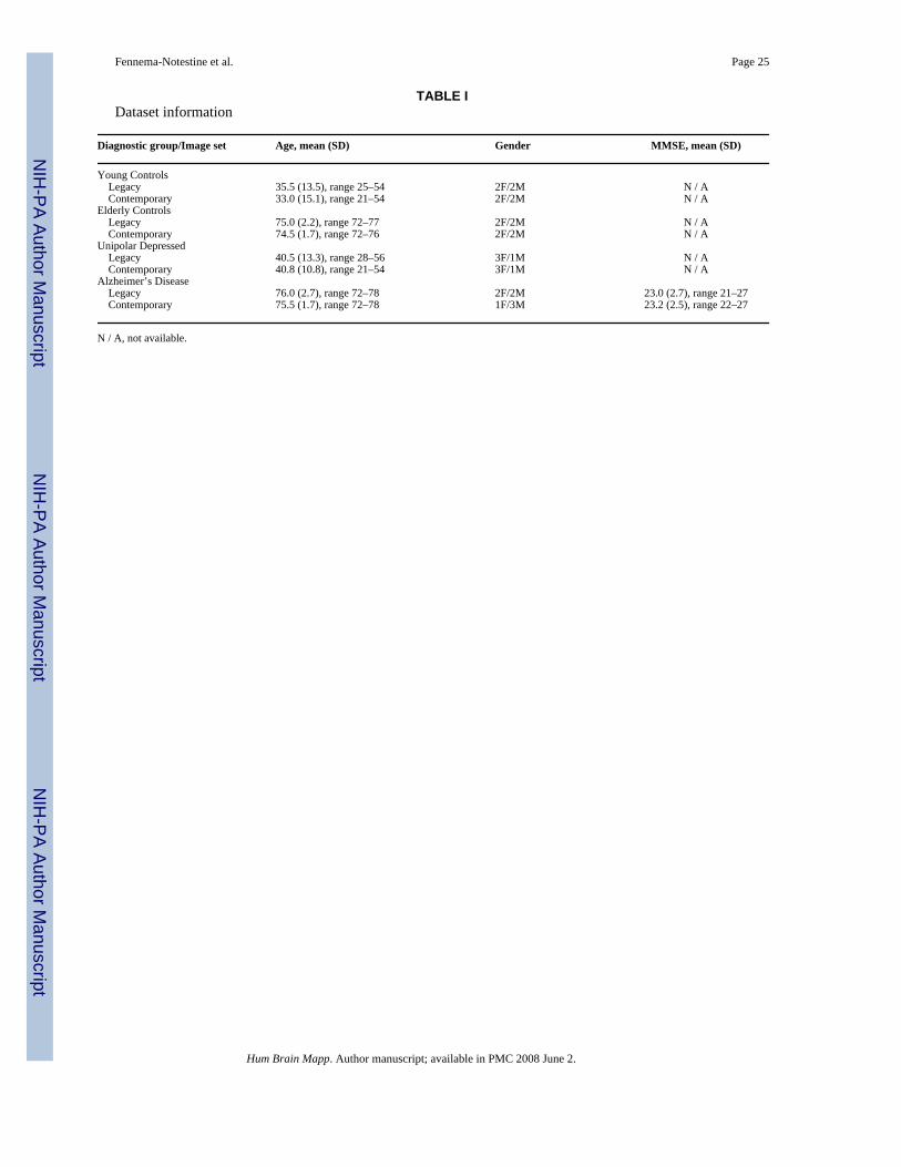
Data collected using two common structural gradient-echo (SPGR) T1-weighted pulsesequences were examined. All datasets were collected on a GE 1.5 T magnet at the VA SanDiego Healthcare System MRI Facility that was subjected to regular hardware and softwareupgrades over time. Legacy Datasets were collected over 4 years in the mid- to late-1990s(June of 1994 and July of 1998): TR = 24 ms, TE = 5 ms, NEX = 2, flip angle = 45°, field ofview 24 cm, and contiguous 1.2-mm sections (sagittal acquisition). Contemporary Datasetswere collected between May of 2002 and April of 2003: TR = 20 ms, TE = 6 ms, NEX = 1,flip angle = 30°, field of view 25 cm, and contiguous 1.5-mm sections (sagittal acquisition).Of the 32 datasets examined, 16 were Legacy, and 16 were Contemporary (Table I). TheUniversity of California, San Diego, institutional review board approved all procedures andwritten informed consent was obtained from all subjects.

Diagnostic GroupsFor each MR Image set of 16 datasets, four different diagnostic groups were represented,including depressed (DEPR), Alzheimer’s (AD), young (YNC), and elderly normal controls(ENC), with four subjects from each group (Table I). The YNC and DEPR groups were similarin age and education, as were the ENC and AD groups. Each diagnostic group from Legacyand Contemporary datasets were similar in age and gender, and the AD groups were alsomatched on disease stage as measured with the Mini-Mental State Examination [MMSE,Folstein et al., 1975].

Bias CorrectionTo correct image bias we employed the nonparametric nonuniform intensity normalizationmethod [N3, Sled et al., 1998], which uses a locally adaptive bias correction algorithm. Thismethod was chosen for its applicability to un-skull-stripped image sets and for its excellentperformance compared with other bias correction methods [Arnold et al., 2001]. All 32 datasetswere studied with and without prior bias correction with N3.



NIH


NIH


NIH


https://www.researchgate.net/publication/230302439_The_Distribution_of_Flora_in_the_Alpine_Zone?el=1_x_8&enrichId=rgreq-96bc08e4-cef3-4bad-b85a-28b16633c4a2&enrichSource=Y292ZXJQYWdlOzc3NTgzNTY7QVM6MTAxMTIyOTQ1NTg1MTYwQDE0MDExMjA5OTg0MTI=

https://www.researchgate.net/publication/3192170_Comparing_images_using_the_Hausdorff_distance_IEEE_Trans?el=1_x_8&enrichId=rgreq-96bc08e4-cef3-4bad-b85a-28b16633c4a2&enrichSource=Y292ZXJQYWdlOzc3NTgzNTY7QVM6MTAxMTIyOTQ1NTg1MTYwQDE0MDExMjA5OTg0MTI=

Manual Skull-StrippingTwo anatomists manually skull-stripped six sagittal slices from each raw MR image set toprovide a criterion, or “gold standard,” against which to judge the automated skull-strippingoutcomes. Both anatomists (CPC and SM) were experienced neuroimaging experts withtraining in neuroscience and neuroanatomy. Both anatomists, in collaboration with a trainedneuroanatomist (CFN), completed four sample datasets not included in the present study toformalize a set of criteria for skull-stripping. If anatomists were unable to definitively classifytissue as brain or nonbrain, they were instructed to conservatively include this tissue.Anatomists were provided with all orthogonal views, which provided them with better spatialinformation to make their decisions. Comparisons of the two anatomists manually skull-stripped datasets are examined in the Results section. Six sagittal slices were selected to assessskull-stripping on mid-sagittal slices and on lateral slices passing through the anterior medialtemporal, anterior inferior frontal, posterior cerebellar regions, and posterior occipital regions(Fig. 1). Brain and nonbrain tissues in these regions are often difficult to distinguish on T1-weighted images, particularly in the posterior fossa (Fig. 1, Slices 4–6A) and anterior temporallobe (Fig. 1, Slices 4–6B). The mid-line sections, in addition to including the posterior fossa,often contain cerebrospinal fluid that may be difficult to distinguish from partially volumedadjacent cortex (Fig. 1, Slice 4C,4D).

Automated Methods and Parameter SelectionFor each method except 3dIntracranial (the developer chose not to participate), developers ofthe automated methods were provided with two sample datasets, one young, healthy controlfrom the Legacy image set and one from the Contemporary image set. We asked developersto suggest the most appropriate parameters for the automated application of their softwareusing the image sets provided. These values were used for all analyses in this study. Theselected parameters and the computational processing times are defined within each methoddescription below. The elapsed average processing time per dataset is based on the use of aDell Pentium Xeon 2.2 or 2.4 GHz with 512 MB RAM.

3dIntracranial [3dIntra, Ward, 1999]; in AFNI v. 2.29 [Cox, 1996]—3dIntra, includedin the Analysis of Functional NeuroImage (AFNI) library, involves several steps. First a three-compartment Gaussian model is fit to the intensity histogram. A downhill simplex method isused to estimate means, standard deviations, and weights of presumed gray matter, whitematter, and background compartments. From these estimated values a probability densityfunction (PDF) is derived to set upper and lower signal intensity bounds as a first step to identifybrain voxels. Upper and lower bounds are set to exclude nonbrain voxels. Next, a connectedbrain region within each axial slice is identified by finding the complement of the largestnonbrain region within that slice, under the constraint that the area of connected brain becomessmaller as the segmentation moves from the center of the brain. The union of such connectedbrain regions is formed as this slice-by-slice segmentation is repeated for sagittal and coronalslices. Next, a 3D envelope based on local averaging smoothes brain edges. Finally, brainvoxels with few brain voxel-neighbors are excluded from brain, whereas holes with manybrain-voxel-neighbors are included. 3dIntracranial is integrated in the extensive library ofAFNI image analysis tools and its public source code is freely available athttp://afni.nimh.nih.gov/afni/. The 3dIntracranial parameters utilized in the present study werethe default parameters, described as follows: minimum voxel intensity limit = internalprobability density function (PDF) estimate for lower bound; maximum voxel intensity limit= internal PDF estimate for upper bound; minimum voxel connectivity to enter m = 4;maximum voxel connectivity to leave n = 2; and spatial smoothing of segmentation mask.

Brain Extraction Tool, v. 1.2 [BET, Smith, 2002]—BET employs a deformable modelto fit the brain’s surface using a set of “locally adaptive model forces.” This method estimates



NIH


NIH


NIH


http://afni.nimh.nih.gov/afni/

the minimum and maximum intensity values for the brain image, a “center of gravity” of thehead image, and head size based on a spherical equivalent, and subsequently initializes thetriangular tessellation of the sphere’s (head’s) surface. BET v. 1.2 is freely available in theFMRIB FSL Software Library (http://www.fmrib.ox.ac.uk/fsl/). The developer recommendedthe default parameters for automated processing of both the legacy and contemporary images.The parameters utilized in the application herein are the default parameters, described asfollows: fractional intensity threshold = 0.5; vertical gradient in fractional intensity threshold= 0.

Hybrid Watershed Algorithm, v. 1.21 [HWA, Segonne et al., 2004]; in FreeSurfer[Dale et al., 1999; Fischl and Dale, 2000; Fischl et al., 1999]—This HWA method isa hybrid of a watershed algorithm [Hahn and Peitgen, 2000] and a deformable surface model[Dale et al., 1999] that was designed to be conservatively sensitive to the inclusion of braintissue. In general, watershed algorithms segment images into connected components, usinglocal optima of image intensity gradients. HWA uses a watershed algorithm that is solely basedon image intensities; the algorithm, which operates under the assumption of the connectivityof white matter, segments the image into brain and nonbrain components. A deformablesurface-model is then applied to locate the boundary of the brain in the image. A final optionunder development will incorporate an atlas-based analysis to verify the correctness of theresulting surface, modify it if important structures have been removed, and locate the best-estimate boundary of the brain in the image. In HWA v. 1.21 the atlas-based option was notfinalized, resulting in a considerably better performance without the atlas-based option.Therefore, the present study examined HWA without the atlas option. HWA v. 1.21 is freelyavailable as a component of the FreeSurfer software package athttp://surfer.nmr.mgh.harvard.edu/. HWA developers recommended the default parameters forautomated processing of both legacy and contemporary images. The parameters utilized in thisstudy are the hard-coded default parameters of HWA without the atlas option.

Brain Surface Extractor v. 3.3 [BSE, Sandor and Leahy, 1997; Shattuck et al.,2001]—BSE, designed to fit the surface of all CNS regions, including the spinal cord, uses asequence of anisotropic diffusion filtering, Marr-Hildreth edge detection, and morphologicalprocessing to segment the brain within whole-head MRI. In MRI of the brain the boundarybetween the brain and the skull will produce a contour in the Marr-Hildreth edge detectionresult. Additional gradients in the image may otherwise act as decoys for automated methods;for this reason, BSE uses anisotropic diffusion filtering [Perona and Malik, 1990]. This is aspatially adaptive edge-preserving filtering technique that smoothes small image gradientswhile preserving larger variations that correspond to strong edges in the image. Because ofnoise in the image and actual anatomic connections such as optic tracts, the brain contour thatBSE generates may not separate the brain from the rest of the head. BSE breaks remainingconnections between the brain and the other tissues in the head using a morphological erosionoperation. After identifying the brain using a connected component operation, BSE applies acorresponding dilation operation to undo the effects of the erosion. As a final step, BSE appliesa morphological closing operation that fills small pits and holes that may occur in the brainsurface. BSE v. 3.3 is freely available for download from the BrainSuite website,http://neuroimage.usc.edu/brainsuite/. The developers recommended the following parametersfor automated processing of both legacy and contemporary image sets: anisotropic filter = 5iterations with 5.0 diffusion constant; edge detector kernel = 0.8 sigma. These parameters wereutilized in this study.

Statistical AnalysesData analytic methods included the following: 1) the comparison of two manual anatomists’performance using the Jaccard similarity coefficient (JSC) to measure degree of



NIH


NIH


NIH


http://www.fmrib.ox.ac.uk/fsl/

http://surfer.nmr.mgh.harvard.edu/

http://neuroimage.usc.edu/brainsuite/

https://www.researchgate.net/publication/3191811_Scale-space_and_edge_detection_using_anisotropic_diffusion_IEEE_Tran_PAMI?el=1_x_8&enrichId=rgreq-96bc08e4-cef3-4bad-b85a-28b16633c4a2&enrichSource=Y292ZXJQYWdlOzc3NTgzNTY7QVM6MTAxMTIyOTQ1NTg1MTYwQDE0MDExMjA5OTg0MTI=

https://www.researchgate.net/publication/221402032_The_Skull_Stripping_Problem_in_MRI_Solved_by_a_Single_3D_Watershed_Transform?el=1_x_8&enrichId=rgreq-96bc08e4-cef3-4bad-b85a-28b16633c4a2&enrichSource=Y292ZXJQYWdlOzc3NTgzNTY7QVM6MTAxMTIyOTQ1NTg1MTYwQDE0MDExMjA5OTg0MTI=

correspondence, or overlap, for each image slice; 2) detailed qualitative review of all outcomes;3) the comparison of each manually skull-stripped outcome (the criterion) to the outcome ofeach automated method using JSC to measure the degree of correspondence for each slice[Jaccard, 1912; Zou et al., 2004a,b]; 4) a similar comparison of methods with the Hausdorffdistance measure [Huttenlocher et al., 1993] to examine the degree of mismatch between thecontours (or shape) of two image sets; and 5) the comparison of the sensitivity and specificityof all methods (including both manual sets) derived from an Expectation-Maximization (EM)algorithm [STAPLE, Warfield et al., 2004; Zou et al., 2004b], which provides a maximumlikelihood estimate of the underlying brain prototype inferred from the results of all skull-stripping methods.

Jaccard Similarity Comparison—The JSC is formulated as:

where A is the area of brain region of the manually skull-stripped image slice (criterion) andB is the area of brain region of the corresponding image slice skull stripped using the comparedskull-stripping tool [Jaccard, 1912; Zou et al., 2004a,b]. A JSC of 1.0 represents completeoverlap or agreement, whereas an index of 0.0 represents no overlap. At both extremes, thisJSC is similar to the Dice similarity coefficient, which is a simple transform. First, JSC wasemployed to describe the overall level of similarity between the two manual outcomes byexpressing the overlap between each pair of slices. Second, the results of the four automatedskull-stripping tools (with and without bias correction) were compared to the manually strippedslices.

Hausdorff distance image comparison—We applied Hausdorff distance measures[Huttenlocher et al., 1993] to examine the degree of mismatch between the contours of twoimage sets (A and B). This measure reflects the distance of the point in A that is farthest fromany point of B and vice versa. Given two finite point sets A = {a1, …,ap} and B = {b1, …,bq}, where A and B are sets of points on the contour of a skull-stripped brain slice. TheHausdorff distance is defined as:

The directed Hausdorff distance from A to B h(A,B) is defined as:

Here the norm is L2 or Euclidean norm, where h(A,B) and h(B,A) are asymmetrical distances.

Since Hausdorff distance measures the extent to which each point of a particular image pointset lies near some point of another image point set, it can be used to determine the degree ofresemblance between two objects superimposed on one another. For the Hausdorff distanced, every point of A must be within a distance d of some point of B and vice versa. The maximumdisplacement for the Hausdorff measure is calculated for each image comparison, A and B.For example, in Figure 4 (right panels), the distance from each point on the yellow contour (A:manual strip) to each point on the red contour (B: automated strip) is calculated. In ourestimation of the Hausdorff distance, we adjusted the calculations to exclude outliers; if onlya very few points are far from average, these extreme distances would not meaningfullyrepresent common method performance. That is, the distance measure would not berepresentative of the common features resulting from automated application. In the presentapplication of the Hausdorff measure, the algorithm first orders the boundary points distances(in ascending order). The 25th and 75th percentiles are then estimated for image A and B andthe interquartile range (IQR) for image A and B is estimated. The IQR is equal to the boundarypoint distance at the 75th percentile less the boundary point distance at the 25th percentile. The



NIH


NIH


NIH






present comparison utilized the upper inner fence as defined by the boundary point distance atthe 75th percentile plus 1.5*IQR [Tukey, 1977]. This fence is used as a more robust normaloutlier boundary than maximum distance in Hausdorff calculations yielding a modifiedHausdorff measure likely to be less sensitive to measurement error.

Expectation-maximization (EM) comparison—Warfield et al. [2004] developed an EMalgorithm, named STAPLE, for computing a probabilistic estimate of the ground-truthsegmentation from a group of expert segmentations, and a simultaneous measure of the qualityof each expert. As we applied their algorithm, this measure is a maximum likelihood estimateof the underlying agreement among all of the skull-stripping methods (two manual plus fourautomated both with and without bias correction). The underlying agreement is represented byan unobserved or hidden skull-stripped prototype that divides all voxels into brain or nonbrainsets, a hidden, binary ground truth segmentation.

The iterative log-likelihood maximization algorithm estimates specificity and sensitivityparameters given a priori probabilities of hidden binary ground truth segmentation and initialestimates of specificity and sensitivity. The sensitivity of an expert j expressed as a proportionpj, where ({pj} ∈[0,1]), is the relative frequency of an expert decision that a voxel belongs tothe brain region when the ground truth for that voxel also indicates the same decision. Thespecificity of an expert j expressed as a proportion qj, where ({qj} ∈[0,1]), is the relativefrequency of an expert decision that a voxel does not belong to the brain region when the groundtruth for that voxel also indicates the same decision. The a priori probabilities for all the voxelsfor each slice of each subject tested are set to 0.5, indicating no initial knowledge about groundtruth. The initial estimates for sensitivity and specificity are all set to 0.9. The terminationcriterion for convergence set the root mean square error to < 0.005.

Statistical summary—We employed mixed model analyses with the conventional alphalevel of 0.05 for a significant statistical effect. Partial eta-squared (η2) values are provided asan estimate of effect size. Between-subjects effects were examined for Image Set (Legacy,Contemporary) and Diagnostic Group (YNC, ENC, DEPR, and AD). Univariate within-subjects repeated measures effects were examined for Slice (Slices 1 through 6 as in Fig. 1),Bias Correction (with and without N3 correction), and Method (3dIntra, BET, BSE, and HWA).These univariate analyses employed the Huynh-Feldt correction since sphericity could not beassumed; logarithmic transforms of the same data produced similar findings. Both within- andbetween-group post-hoc analyses contrasted pairs of each condition in sequence. For example,post-hoc analyses of Diagnostic Group included three comparisons: YNC vs. DEPR, DEPRvs. ENC, ENC vs. AD. To analyze agreement between raters we performed a Slice by ImageSet by Diagnostic Group mixed design analysis of variance (ANOVA) using JSC as thedependent variable. Investigation of the influence of study variables on the correspondence ofeach automated method with each manual outcome comparison required a Method by BiasCorrection by Slice by Image Set by Diagnostic Group mixed design (ANOVA) with the JSCand the modified Hausdorff measure analyzed as separate dependent variables. The latterANOVA design also was used to investigate the influence of study variables on EM-derivedsensitivity and specificity. EM analyses reported herein included all four automated methodsand the two manual outcomes.

RESULTSStatistical Comparison of Two Manually Stripped Outcomes

When the two anatomists’ manually stripped sections were compared, the grand mean JSCaveraged across slices was 0.938 (SE = 0.002). There were significant main effects of Slice(F(4.5, 108.5) = 18.5, P < 0.001, partial η2 = 0.44) and Diagnostic Group (F(3,24) = 7.2, P =



NIH


NIH


NIH


0.001, partial η2 = 0.47). Neither the effect of Image Set nor any interactions reachedsignificance (all P > 0.05; all partial η2 < 0.13). Post-hoc, within-subjects contrasts suggestedthat the similarity coefficient was lowest for the two mid-line sagittal sections (Fig. 1, Slices3, 4) relative to the four lateral sections; these mid-line sections were most variable betweenanatomists. As predicted, contrasts for Diagnostic Group suggested that the similaritycoefficients were lower for ENC and AD groups relative to the YNC and DEPR subjects (F(3,24) = 7.2, P = 0.001, partial η2 = 0.47). Specifically, the coefficients for the YNC and DEPRgroups did not differ (P > 0.05) and neither did the ENC and AD groups (P > 0.05). Thesimilarity coefficients for the DEPR and ENC groups, however, were significantly different(P = 0.001). In summary, the brain contours drawn by anatomists agreed less in the two mesialslices and for data from the older diagnostic groups. These conditions that were more difficultfor manual skull-stripping may also prove difficult for the automated methods.

Qualitative Evaluation of All OutcomesQualitative review of all individual results revealed that the outcomes differed in: 1) the amountof cerebrospinal fluid (CSF) included in the stripped volume; 2) the type of nonbrain remainingin the stripped volume; and 3) the regions and extent of brain tissue loss in the stripped volume.All methods included internal (e.g., ventricular) CSF in the resulting volume, which wouldallow future processing to evaluate ventricular volume. HWA consistently included externalCSF in the space between brain tissue and the external dura (subarachnoid space; HWA in Fig.2).

The type and extent of nonbrain tissue remaining in the stripped volumes varied across methodsand the most common results are described here (Figs. 2–4). All methods tended to leave somenonbrain tissue in the posterior fossa (Fig. 2). As intended by developers, BSE volumesconsistently include the spinal cord (Fig. 2). BET tended to leave muscle and other tissue inthe mid-neck region (Figs. 2–4). On some occasions, nonbrain included in 3dIntra results wasfound in similar areas, although to a lesser extent. HWA volumes consistently includedsurrounding subarachnoid space and nonbrain dura (Figs. 2–4), occasionally including tissuearound the eyes (Fig. 2), although HWA consistently removed nonbrain tissues in the neckregions.

The region and extent of brain tissue loss in stripped volumes also varied across methods (Figs.3, 4). HWA was sensitive to retaining brain volume. On one occasion, however, the cerebellarvolume was reduced. In general, the anterior frontal cortex, anterior temporal cortex, posterioroccipital cortex, and cerebellar areas were common locations for loss of cortical voxels in othermethods (3dIntra, BET, and BSE). The most cortical loss on stripped volumes of theContemporary datasets tended to be a thin layer of brain voxels in these areas, with BSEseeming to result in the least amount of tissue loss. In the Legacy datasets, however, the lossof brain tissue was more severe in some cases for these methods.

Statistical Comparisons of Automated MethodsThe average elapsed processing time for performing automated applications per dataset wascalculated for each automated method based on the performance across all 32 datasets.3dIntracranial required less than 1 min (53.9 s; SD = 10.5), BET required less than 4 min (223.1s; SD = 60.0), HWA required less than 8 min (473.6 s; SD = 127.8), and BSE required on theorder of 15 sec (14.2 s; SD = 0.8).

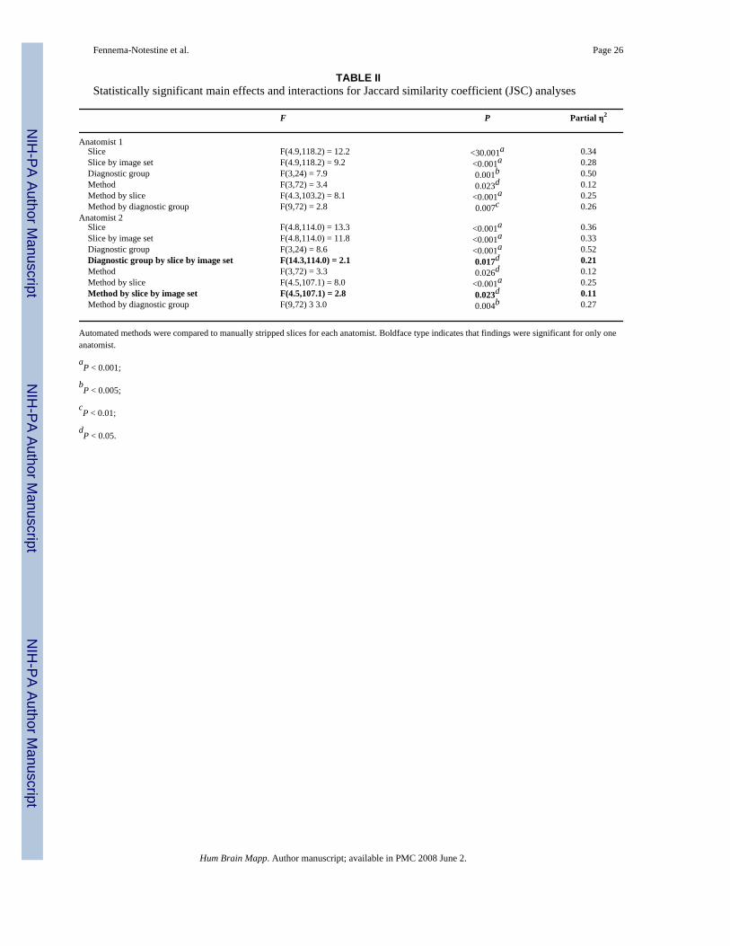
The effects of each condition (Image Set, Slice, Bias Correction, and Diagnostic Group) aredescribed separately, followed by a description of the Method effects and interactions.Statistical results for significant findings are reported for JSC (Table II), Hausdorff distance(Table III), and EM Sensitivity and Specificity (Table IV). JSC and Hausdorff distance analyses



NIH


NIH


NIH


were completed for each anatomist separately. Findings were similar for both anatomists unlessotherwise reported; the representative findings for Anatomist 1 (CC) are reported herein forsimplicity. EM analyses represent the inclusion of all four automated methods and the twomanual outcomes. All results described emphasize the comparison of methods.

Image set—There were no significant differences of JSC or Hausdorff distance between theImage Sets studied (Legacy vs. Contemporary) when the contour of either rater was used asthe ground truth (Anatomist 1: JSC partial η2 = 0.03, Hausdorff partial η2 = 0.12; Anatomist2: JSC partial η2 = 0.01, Hausdorff partial η2 = 0.10). Thus, the correspondence of eachanatomist’s brain contour to the contours produced by the four automated skull-strippingprograms was similar for the two Image Sets. EM analyses, however, revealed a significanteffect of Image Set for Sensitivity (Table IV); the effect did not reach significance forSpecificity (F(1,24) = 3.5, P = 0.074, partial η2 = 0.13). The Contemporary data resulted ingreater sensitivity (mean = 0.960, SE = 0.009) relative to the legacy data (mean = 0.926, SE =0.009). Interactions between Image Set and other conditions are described below.

Slice (regional anatomy)—Significant main effects of Slice were found across all measures(Tables II–IV). The effects of Slice were similar to those found in the comparison of the twoanatomists’ manual skull-stripping results; that is, in general the two midline slices (Fig. 1,Slices 3, 4) had lower similarity coefficients and higher distance measures relative to the morelateral slices. Slice significantly interacted with Image Set for JSC (Table II) and measures ofSensitivity and Specificity yielded by the EM algorithm (Table IV). Mesial slices from Legacydata were least similar to the criterion dataset, whereas mesial (Fig. 1, Slices 3, 4) and mostlateral (Fig. 1, Slices 1, 6) slices from Contemporary data were least similar. Specificity wasbest moving from mesial to lateral slices, particularly for the Contemporary data.

Bias correction—There was no significant main effect of bias correction for any of themeasures (all partial η2 < 0.05), and no interactions with bias correction reached significance.Although there were some individual cases that qualitatively appeared to benefit from biascorrection, this effect was not significant over any condition.

Diagnostic group—The main effect of Diagnostic Group reached significance for allmeasures (Tables II–IV). Planned contrasts supported the hypothesis that all measures weresignificantly poorer for the AD group relative to all other groups. The YNC and DEPR groupsdid not differ significantly, and, unexpectedly, neither did the DEPR and ENC groups. TheJSC for Anatomist 2 resulted in a significant Diagnostic Group by Slice by Image Setinteraction (Table II), although this interaction did not reach significance for Anatomist 1 (F(14.8, 118.2) = 1.5, P = 0.12, partial η2 = 0.16). This 3-way interaction is difficult to interpret,but it appears to suggest that the Contemporary data may result in better performance for themesial slices for the older Diagnostic Groups. Diagnostic Group did not significantly interactwith Image Set, Slice, or Bias Correction for any other measures. Interactions involving Methodare examined below.

Automated methods—Direct evaluation of the four automated skull-stripping methods(Table V) revealed consistent differences for JSC (Table II; analyses compared automatedperformance to manual method) and EM Sensitivity (Table IV; analyses included all automatedand manual methods) measures (but not EM Specificity or Hausdorff indices). Post-hoc JSCcontrasts for Method indicated that 3dIntra and BET did not differ significantly and neitherdid BSE and HWA. BET and BSE, however, were significantly different (P = 0.003). That is,BSE and HWA produced higher similarity measures than 3dIntra and BET for both anatomists(Table V). With respect to Sensitivity, 3dIntra, BET, and BSE did not differ significantly,



NIH


NIH


NIH


whereas HWA was significantly more sensitive than BSE (P < 0.001). Thus, HWA wassignificantly more sensitive than all other automated methods (Table V).

For the measure of Sensitivity, Method significantly interacted with Image Set (Table IV). Theperformance of BET was greatly affected by Image Set; BET was least sensitive on the Legacydata with respect to all other methods, but performed better with the Contemporary data. Nosignificant interactions were observed between Image Set and automated Method for othermeasures. The nonsignificant interaction of Image Set with Method accounted for less than6% of the observed variation of JSC or Hausdorff distance.

There were significant Method by Slice interactions for the JSC (Table II) and EM Sensitivity(Table IV). In general, BSE and HWA performed relatively similarly across slices with themesial slices least similar; 3dIntra and BET, both with lower overall similarity coefficients,performed differently across slices. 3dIntra performed most poorly on Slice 1 with an otherwisesimilar pattern to BSE and HWA. BET, in contrast, performed best on Slice 1 and then at aslightly lower level across Slices 2–6. With respect to Sensitivity, HWA performed consistentlyhigh across all slices. Although less sensitive, BSE was also fairly consistent across slices, withthe exception of poor performance on Slice 1. 3dIntra also was least sensitive on Slice 1. BETwas least sensitive for the two mesial slices (Slices 3 and 4).

For the JSC, the Method by Slice by Image Set interaction was significant for Anatomist 2(Table II), although this interaction did not reach significance for Anatomist 1 (P = 0.11, partialη2 = 0.08). This 3-way interaction, however, was also significant for EM Sensitivity (TableIV).

Of considerable interest, the effect of Diagnostic Group on JSC and Hausdorff distance variedby automated skull-stripping method for both anatomists (Figs. 5, 6; Tables II, III). For EMSpecificity, although there was no significant main effect of Method (partial η2 = 0.039; TableV), there was a significant interaction between Method and Diagnostic Group (Table IV; Fig.7). EM Sensitivity, in contrast, did not significantly interact with Diagnostic Group, althoughthe main effects of Diagnostic Group and Method were both significant (Table IV; Fig. 8). Ofcritical interest, the post-hoc analyses of the interactions between Method and DiagnosticGroup revealed that when compared with BSE and HWA, 3dIntra had significantly lowersimilarity and larger distance coefficients for the AD data, and BET had lower similarity andlarger distance coefficients for the ENC and AD data (Figs. 5, 6). Thus, BSE and HWA weremore effective at finding the brain contour for the AD group, the most challenging group toskull strip. However, 3dIntra was most effective for young normal controls. With respect toEM Specificity (Fig. 7), 3dIntra demonstrated significantly worse performance in AD relativeto other groups, and BSE tended to perform best across all diagnostic groups (Fig. 7). Insummary, the HWA algorithm most successfully retained “true” brain tissue even within theAD group (Table V; Fig. 8), whereas BSE resulted in the best specificity across all conditions(Fig. 7).

DISCUSSIONThis collaborative study provides guidance to end-users and developers of automated skull-stripping applications and demonstrates a quantitative analysis path for the evaluation ofmorphometric analysis tools. The investigation examined the effects of bias correction, imageset, slice location, and diagnostic group on automated skull-stripping performance. Biascorrection of field inhomogeneities through the use of N3 [Sled et al., 1998] did notsignificantly improve performance of skull-stripping methods. Given that some individualcases of these 1.5 T data did improve with prior bias correction, bias correction on data fromhigher-field strength magnets may have a more significant effect. Performance was, in general,



NIH


NIH


NIH


better on the Contemporary data relative to the Legacy data with respect to sensitivity, perhapsdue to improved image contrast. As predicted, mesial brain slices proved the most challengingto skull-strip. These slices included posterior fossa tissue that is often difficult to distinguishfrom adjacent brain tissue, as well as voxels containing partially volumed tissues and CSF(Figs. 2–4). Across all of our performance measures, images from the Alzheimer’s disease(AD) group proved the most difficult to skull strip.

In general, HWA [Segonne et al., 2004] and BSE [v. 3.3, Sandor and Leahy, 1997; Shattucket al., 2001] were more robust across all study conditions relative to 3dIntracranial [Ward,1999] and BET [Smith, 2002], although the interactions between Method and other conditionswarrant further discussion. It should be noted that BSE’s final outcome purposefully aims tofit the brain surface and includes the spinal cord as part of the CNS, whereas HWA aims toconservatively bound the pial surface. Consistent with a recent study [Segonne et al., 2004],HWA was significantly more sensitive than other methods, resulting in a conservative stripthat rarely removed any brain tissue. HWA preserved much of the subarachnoid space, whichmight allow the estimation of cranial vault volume to be incorporated into statistical analysescontrolling for individual differences in head size. However, as with all methods’ results, thefinal outcome would likely benefit from additional editing due to the extent of remainingnonbrain tissue. BSE, in contrast, was more specific, although some brain voxels tended to beremoved, and the final outcomes include some of the same posterior nonbrain regions as inHWA although to a lesser extent.

The significant interaction between Method and Diagnostic Group supported the robust,general application of HWA and BSE relative to 3dIntracranial and BET. However, for theYoung Control (YNC) group, 3dIntracranial produced results that were the most similar to thecriterion dataset and tended to be the most specific. As measured by inclusion of nonbraintissue (false-positives) and exclusion of brain tissue (false-negatives), 3dIntracranial performedpoorly on the data from the AD group, suggesting that 3dIntracranial may be an appropriatetool particularly for younger populations. BET also performed less well for both the ENC andAD data, including neck regions of nonbrain tissue, as in a recent study [Boesen et al., 2004],and removing some anterior and posterior cortical tissue. BSE and HWA, in contrast, were lessaffected by diagnostic group, despite lower similarity coefficients on the YNC data relative to3dIntracranial. In short, 3dIntracranial performed extremely well when working with youngsubject data; however, in the study of older subjects BSE and HWA appeared more promising.The HWA algorithm demonstrated the highest sensitivity, most successfully retaining braintissue even within the AD group, and BSE demonstrated the best specificity in the older groups.

The performance of BSE relative to BET was not easily predictable based on previous studiesof automated application of these methods [Boesen et al., 2004; Lee et al., 2003; Smith,2002]. Although Lee et al. [2003] and Smith [2002] reported that BET performed better thanBSE, Segonne et al. [2004] suggested that BSE may provide superior results. Boesen et al.’s[2004] findings suggested that the relative performance of BET and BSE may be influencedby image quality. The present study differed from previous work in that we employed a morerecent version of the BSE software (v. 3.3), the parameters employed were determined by theexpert developers, and anisotropic filtering was included in the BSE path of the present study,a processing step not always included in other studies [e.g., Smith, 2002].

Our study focused only on T1-weighted image sets and was limited to rectangular k-spacetrajectories. Method performance on other types of image sets may be quite different. As with3dIntracranial and BSE, BET has the ability to strip other types of image sets and might performespecially well on T2- or proton-density-weighted image sets not examined herein [Smith,2002]. Our preliminary work suggests that there are significant challenges to the applicationof these methods to spiral trajectories. In addition, the findings reported here are limited to the



NIH


NIH


NIH


https://www.researchgate.net/publication/8487906_Quantitative_comparison_of_four_brain_extraction_algorithms?el=1_x_8&enrichId=rgreq-96bc08e4-cef3-4bad-b85a-28b16633c4a2&enrichSource=Y292ZXJQYWdlOzc3NTgzNTY7QVM6MTAxMTIyOTQ1NTg1MTYwQDE0MDExMjA5OTg0MTI=

specific groups studied. Given our findings in AD, the characteristics of the AD data thatinfluenced the performance of these automated methods should be investigated further, andthese algorithms tested on other neurodegenerative groups. Finally, this study provides noinformation about region-growing algorithms and other hybrid approaches, which performedwell in previous studies of skull-stripping methods [e.g., Boesen et al., 2004; Lee et al.,2003].

The comprehensive analysis path employed in the present study provides several quantitativemeasures that may be useful to future studies of image processing. The initial JSC analyses[Jaccard, 1912; Zou et al., 2004a,b] are similar to previously employed statistics. Theseprovided general information on the amount of overlap between two outcomes, although therewas no specific information as to the sensitivity, specificity, or shape differences that may beadditionally informative. Our estimation of the Hausdorff distance measure [Huttenlocher etal., 1993] provided information on shape differences between outcomes, although in the presentstudy the results were similar to the Jaccard findings. When this measure is small the shapesare similar and almost exactly overlap. When this measure increases the shapes may be quitedissimilar, despite overlap. Most important to the present work, the use of the Expectation-Maximization (EM) algorithm [Warfield et al., 2004; Zou et al., 2004b] provided bothsensitivity and specificity indices for the methods examined, including the manual outcomes,relative to the overall ground truth. This additional information was critical to informingdifferences between BSE, a more specific method, and HWA, a more sensitive method, bothof which performed similarly well across diagnostic groups on the other similarity measures.

CONCLUSIONSEvidence suggests that HWA may remove substantial nonbrain tissue from the difficult faceand neck regions, carefully preserving the brain, although the outcome often would benefitfrom further stripping of other nonbrain regions; BSE, in contrast, more clearly reaches thesurface of the brain, although, in some cases, some brain tissue may be removed. 3dIntracranialand BET often left large nonbrain regions and/or removed some brain regions, particularly inthe older populations. Based on the present findings, further investigations may pursue a skull-stripping approach that combines methods, either sequentially or in parallel. For example,HWA simplifies the problem of stripping away nonbrain while proving to be quite sensitive,and following the application of HWA with BSE may improve the specificity of the final result.Another approach presented recently [Rex et al., 2003] pursued the possibility of combiningmethods within a single meta-algorithm to optimize results. Again, the present study aimed toexamine the automated performance of available skull-stripping methods only on T1-weightedimage sets. All methods examined in the present study permit users to manually optimizeparameters, which may improve performance over values employed herein. These parameterchoices may vary depending on the region of interest to the investigators, as some regions maybe more susceptible to tissue loss with some methods. Furthermore, BSE, BET, and3dIntracranial are applicable to some other types of image sets (e.g., T2-weighted), and thusmight be significantly advantageous under such circumstances. We hope this study will guideend-users toward a method appropriate to their datasets, improve efficiency of processing forlarge, multisite neuro-imaging studies, and provide insight to the developers for future work.

Acknowledgements

Preliminary findings related to this work were presented at the Society for Neuroscience 2003 meeting (Fennema-Notestine et al. 2003). We thank Jonathan Sacks, Ph.D., and Simon K. Warfield, Ph.D., of Harvard Medical Schooland the Surgical Planning Lab of Brigham and Women’s Hospital for direction to the Expectation-Maximizationmethodology that considerably improved our analysis path. We also thank Randy Gollub, M.D., Ph.D., and JorgeJovicich, Ph.D., both Morphometry BIRN investigators at the MGH/MIT/HMS Martinos Center for BiomedicalImaging, for their unwavering support of this project.



NIH


NIH


NIH



Contract grant sponsor: National Center for Research Resources at the National Institutes of Health (NIH); Contractgrant number: U24 RR021382 (to the Morphometry Biomedical Informatics Research Network, BIRN,http://www.nbirn.net) and Projects BIRN002 and BIRN004, M01RR00827, P41-RR14075, R01 RR16594-01A1,P41-RR13642; Contract grant sponsor: National Institute of Mental Health at NIH; Contract grant numbers:5K08MH01642; R01MH42575; HIV Neurobehavioral Research Center MH45294; Contract grant sponsor: NationalInstitute on Aging at NIH; Contract grant numbers: R01 AG12674; AG04085; Contract grant sponsor: San DiegoAlzheimer’s Disease Research Center; Contract grant number: P50AGO5131; Contract grant sponsor: NationalInstitute for Biomedical Imaging and Bioengineering (NIBIB) at NIH; Contract grant number: R01 EB002010;Contract grant sponsor: Mental Illness and Neuroscience Discovery (MIND) Institute; Contract grant sponsor:Department of Veterans Affairs Medical Research Service; Contract grant numbers: VA Merit Review and ResearchEnhancement award programs.

ReferencesArnold JB, Liow JS, Schaper KA, Stern JJ, Sled JG, Shattuck DW, Worth AJ, Cohen MS, Leahy RM,

Mazziotta JC, et al. Qualitative and quantitative evaluation of six algorithms for correcting intensitynonuniformity effects. Neuroimage 2001;13:931–943. [PubMed: 11304088]

Boesen K, Rehm K, Schaper K, Stoltzner S, Woods R, Luders E, Rottenberg D. Quantitative comparisonof four brain extraction algorithms. Neuroimage 2004;22:1255–1261. [PubMed: 15219597]

Cox RW. AFNI: software for analysis and visualization of functional magnetic resonance neuroimages.Comput Biomed Res 1996;29:162–173. [PubMed: 8812068]

Dale AM, Fischl B, Sereno MI. Cortical surface-based analysis. I. Segmentation and surfacereconstruction. Neuroimage 1999;9:179–194. [PubMed: 9931268]

DeCarli C, Maisog J, Murphy DG, Teichberg D, Rapoport SI, Horwitz B. Method for quantification ofbrain, ventricular, and subarachnoid CSF volumes from MR images. J Comput Assist Tomogr1992;16:274–284. [PubMed: 1545026]

Fennema-Notestine, C.; Ozyurt, IB.; Brown, GG.; Clark, CP.; Morris, S.; Bischoff-Grethe, A.; Bondi,MW.; Jernigan, TL. the Human Brain Morphometry BIRN. Bias correction, pulse sequence, andneurodegeneration influence performance of automated skull-stripping methods. In: Washington, D.,editor. Program No. 863.23 Abstract Viewer/Itinerary Planner. New Orleans, LA: 2003. Online

Fischl B, Dale AM. Measuring the thickness of the human cerebral cortex from magnetic resonanceimages. Proc Natl Acad Sci U S A 2000;97:11050–11055. [PubMed: 10984517]

Fischl B, Sereno MI, Dale AM. Cortical surface-based analysis. II. Inflation, flattening, and a surface-based coordinate system. Neuroimage 1999;9:195–207. [PubMed: 9931269]

Folstein MF, Folstein SE, McHugh PR. Mini-mental state.” A practical method for grading the cognitivestate of patients for the clinician. J Psychiatr Res 1975;12:189–198. [PubMed: 1202204]

Hahn H, Peitgen H-O. The skull stripping problem in MRI solved by a single 3D watershed transform.Paper presented at the Proc MICCAI, LNCS 2000;1935:134–143.

Hand, DJ.; Mannila, H.; Smyth, P. Principles of data mining. Cambridge, MA: Bradford Book, MITPress; 2001.

Huttenlocher DP, Klanderman GA, Rucklidge WJ. Comparing images using the hausdorff distance. IEEETrans Pattern Anal Machine Intell 1993;15:850–863.

Jaccard P. The distribution of flora in the alpine zone. New Phytol 1912;11:37–50.Lee JM, Yoon U, Nam SH, Kim JH, Kim IY, Kim SI. Evaluation of automated and semi-automated skull-

stripping algorithms using similarity index and segmentation error. Comput Biol Med 2003;33:495–507. [PubMed: 12878233]

Perona P, Malik J. Scale-space and edge detection using anisotropic diffusion. IEEE Trans Pattern AnalMachine Intell 1990;12:629–639.

Rex, DE.; Shattuck, DW.; Woods, RP.; Stoltzner, SE.; Toga, AW. Meta-algorithm for automated brainextraction from a structural MRI. In: Washington, D., editor. Program No. 863.24 Abstract Viewer/Itinerary Planner. New Orleans, LA: 2003. Online

Sandor S, Leahy R. Surface-based labeling of cortical anatomy using a deformable database. IEEE TransMed Imaging 1997;16:41–54. [PubMed: 9050407]

Segonne F, Dale AM, Busa E, Glessner M, Salat D, Hahn HK, Fischl B. A hybrid approach to the skullstripping problem in MRI. Neuroimage 2004;22:1060–1075. [PubMed: 15219578]



NIH


NIH


NIH


http://www.nbirn.net

Shattuck DW, Sandor-Leahy SR, Schaper KA, Rottenberg DA, Leahy RM. Magnetic resonance imagetissue classification using a partial volume model. Neuroimage 2001;13:856–876. [PubMed:11304082]

Sled JG, Zijdenbos AP, Evans AC. A nonparametric method for automatic correction of intensitynonuniformity in MRI data. IEEE Trans Med Imaging 1998;17:87–97. [PubMed: 9617910]

Smith SM. Fast robust automated brain extraction. Hum Brain Mapp 2002;17:143–155. [PubMed:12391568]

Tukey, JW. Exploratory data analysis. Reading, MA: Addison-Wesley; 1977.Ward, BD. Intracranial segmentation. Milwaukee: Biophysics Research Institute, Medical College of

Wisconsin; 1999. AFNI is NIH supported software at http://afni.nimh.nih.gov/afni/index.shtmlWarfield SK, Zou KH, Wells WM. Simultaneous truth and performance level estimation (STAPLE): an

algorithm for the validation of image segmentation. IEEE Trans Med Imaging 2004;23:903–921.[PubMed: 15250643]

Zou KH, Warfield SK, Bharatha A, Tempany CM, Kaus MR, Haker SJ, Wells WM 3rd, Jolesz FA,Kikinis R. Statistical validation of image segmentation quality based on a spatial overlap index. AcadRadiol 2004a;11:178–189. [PubMed: 14974593]

Zou KH, Wells WM 3rd, Kikinis R, Warfield SK. Three validation metrics for automated probabilisticimage segmentation of brain tumours. Stat Med 2004b;23:1259–1282. [PubMed: 15083482]



NIH


NIH


NIH


http://afni.nimh.nih.gov/afni/index.shtml

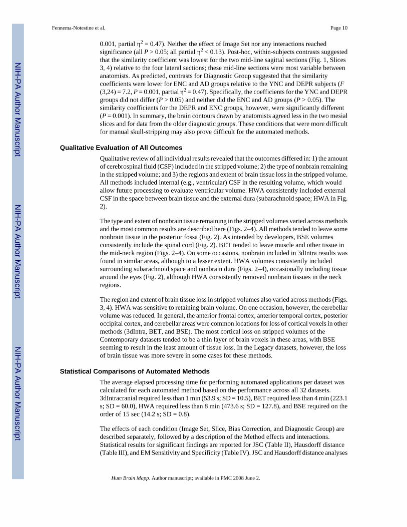
Figure 1.Standard location of the six sagittal, manually stripped slices as demonstrated on a coronalimage. The six sagittal slices represent the criterion dataset; three slices from each hemispherein symmetrical locations passing through regions that are difficult to skull-strip. Slices arenumbered for reference. Three sample images are presented in the sagittal plane. Lettersrepresent difficult regions as referenced in the text.



NIH


NIH


NIH


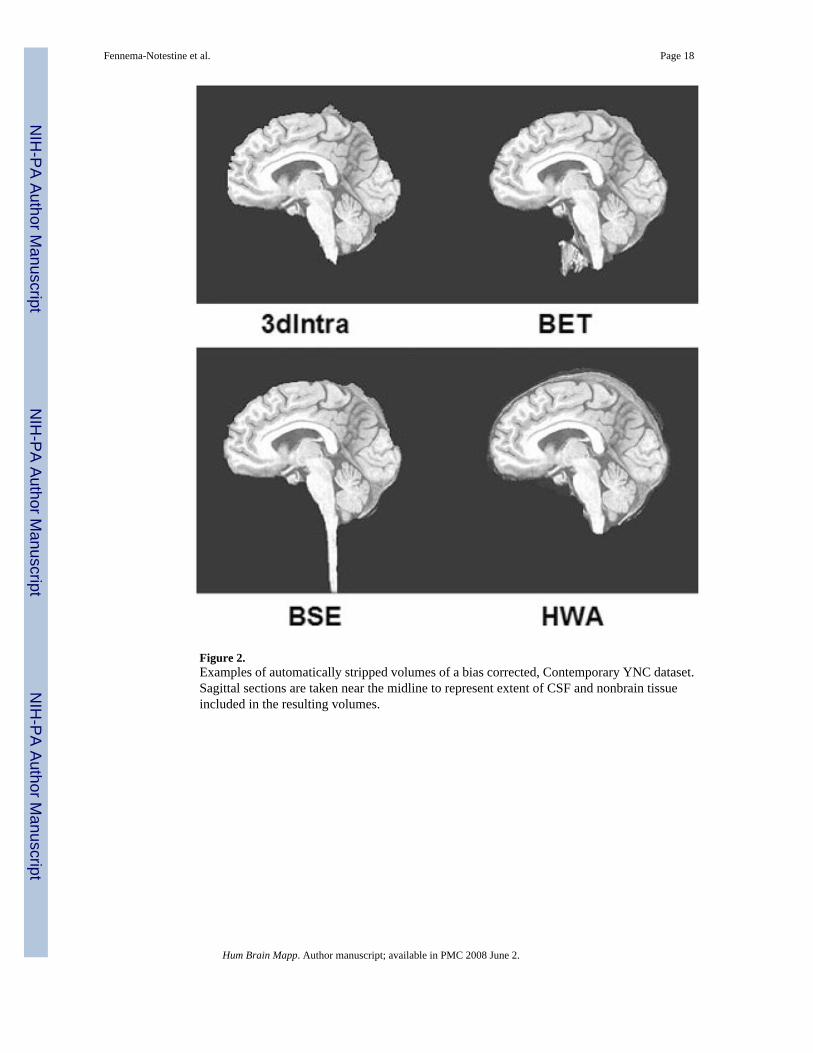
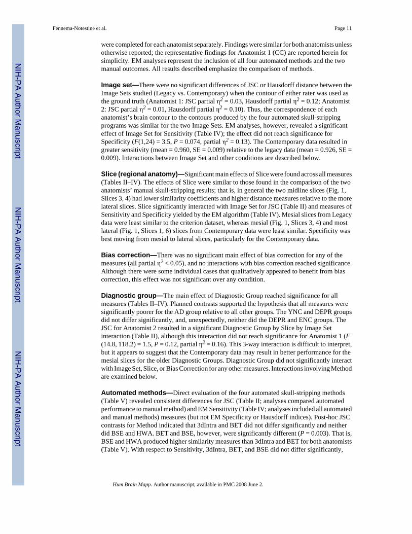
Figure 2.Examples of automatically stripped volumes of a bias corrected, Contemporary YNC dataset.Sagittal sections are taken near the midline to represent extent of CSF and nonbrain tissueincluded in the resulting volumes.



NIH


NIH


NIH


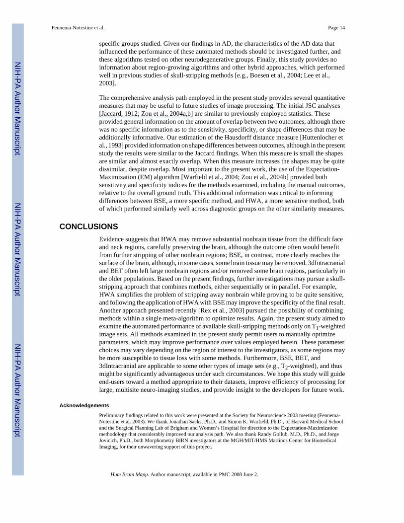
Figure 3.Examples of automatically stripped volumes of a bias corrected, Legacy YNC dataset. Sagittalsections are lateral to the midline and represent the extent of brain tissue retained or excludedfrom the resulting volumes.



NIH


NIH


NIH


Figure 4.Examples of outcomes for a bias corrected, Contemporary ENC dataset. Each pair of figuresincludes solid color overlays on the stripped image (left) and the contours of these shapes(right). Left, Yellow = regions included in the manual but not in the automatic outcome. Blue= regions included in the automatic but not in the manual outcome. Right, Yellow = contourof manually-stripped dataset. Red = contour of automatically stripped dataset.



NIH


NIH


NIH


Figure 5.Mean (std. error bars) Jaccard similarity coefficient (JSC) for Diagnostic Group by Methodrelative to the manually stripped slices from Anatomist 1. Mean JSC for the two manual raters(0.938) is represented by the horizontal dashed black line.



NIH


NIH


NIH


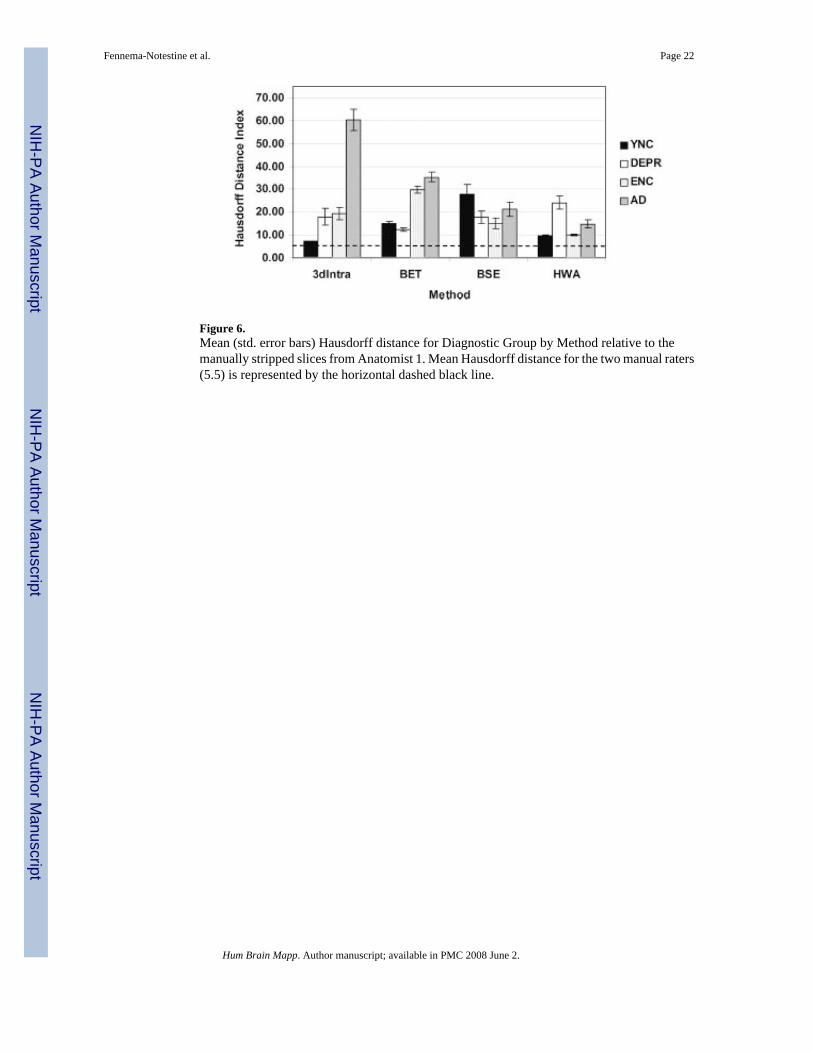
Figure 6.Mean (std. error bars) Hausdorff distance for Diagnostic Group by Method relative to themanually stripped slices from Anatomist 1. Mean Hausdorff distance for the two manual raters(5.5) is represented by the horizontal dashed black line.



NIH


NIH


NIH


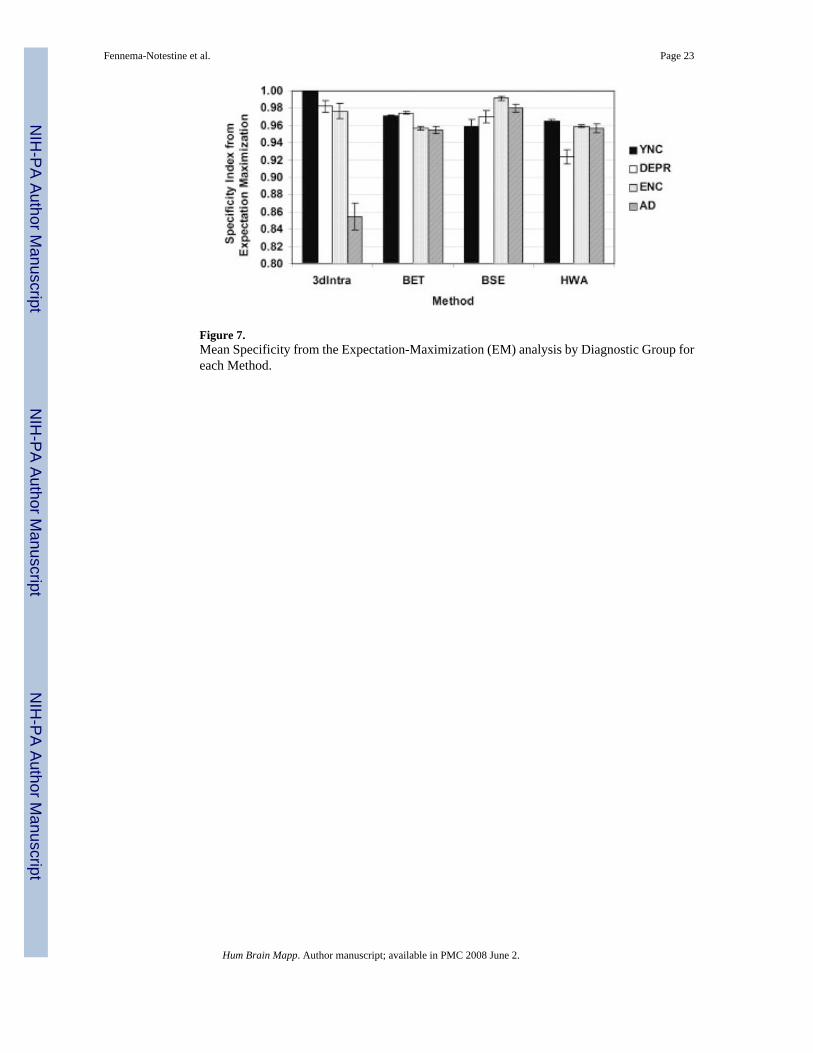
Figure 7.Mean Specificity from the Expectation-Maximization (EM) analysis by Diagnostic Group foreach Method.



NIH


NIH


NIH


Figure 8.Mean Sensitivity from the Expectation-Maximization (EM) analysis by Diagnostic Group foreach Method.



NIH


NIH


NIH


NIH


NIH


NIH



TABLE IDataset information

Diagnostic group/Image set Age, mean (SD) Gender MMSE, mean (SD)

Young Controls Legacy 35.5 (13.5), range 25–54 2F/2M N / A Contemporary 33.0 (15.1), range 21–54 2F/2M N / AElderly Controls Legacy 75.0 (2.2), range 72–77 2F/2M N / A Contemporary 74.5 (1.7), range 72–76 2F/2M N / AUnipolar Depressed Legacy 40.5 (13.3), range 28–56 3F/1M N / A Contemporary 40.8 (10.8), range 21–54 3F/1M N / AAlzheimer’s Disease Legacy 76.0 (2.7), range 72–78 2F/2M 23.0 (2.7), range 21–27 Contemporary 75.5 (1.7), range 72–78 1F/3M 23.2 (2.5), range 22–27

N / A, not available.


NIH


NIH


NIH



TABLE IIStatistically significant main effects and interactions for Jaccard similarity coefficient (JSC) analyses

F P Partial η2

Anatomist 1 Slice F(4.9,118.2) = 12.2 <30.001a 0.34 Slice by image set F(4.9,118.2) = 9.2 <0.001a 0.28 Diagnostic group F(3,24) = 7.9 0.001b 0.50 Method F(3,72) = 3.4 0.023d 0.12 Method by slice F(4.3,103.2) = 8.1 <0.001a 0.25 Method by diagnostic group F(9,72) = 2.8 0.007c 0.26Anatomist 2 Slice F(4.8,114.0) = 13.3 <0.001a 0.36 Slice by image set F(4.8,114.0) = 11.8 <0.001a 0.33 Diagnostic group F(3,24) = 8.6 <0.001a 0.52 Diagnostic group by slice by image set F(14.3,114.0) = 2.1 0.017d 0.21 Method F(3,72) = 3.3 0.026d 0.12 Method by slice F(4.5,107.1) = 8.0 <0.001a 0.25 Method by slice by image set F(4.5,107.1) = 2.8 0.023d 0.11 Method by diagnostic group F(9,72) 3 3.0 0.004b 0.27

Automated methods were compared to manually stripped slices for each anatomist. Boldface type indicates that findings were significant for only oneanatomist.

aP < 0.001;

bP < 0.005;

cP < 0.01;

dP < 0.05.


NIH


NIH


NIH



TABLE IIIStatistically significant main effects and interactions for Hausdorff distance analyses

F P Partial η2

Anatomist 1 Slice F(4.1,98.4) = 23.0 <0.001a .49 Diagnostic group F(3,24) = 4.8 0.010c .37 Method by diagnostic group F(9.0,72.0) = 2.1 0.037c .21Anatomist 2 Slice F(3.9,93.2) = 24.1 <0.001a .50 Diagnostic group F(3,24) = 4.8 0.009b .38 Method by diagnostic group F(9.0,72.0) = 2.1 0.037c .21

Automated methods were compared to manually stripped slices for each anatomist.

aP < 0.001;

bP < 0.01;

cP < 0.05.


NIH


NIH


NIH



TABLE IVStatistically significant main effects and interactions for EM analyses of Sensitivity and Specificity

F P Partial η2

Sensitivity Slice F(3.1,73.7) = 5.4 0.002b 0.18 Image set F(1,24) = 8.3 0.008c 0.26 Slice by image set F(3.1,73.7) = 6.3 0.001b 0.21 Diagnostic group F(3,24) = 5.1 0.007b 0.39 Method F(2.6,63.0) = 12.1 <0.001a 0.33 Method by image set F(2.6,63.0) = 5.0 0.005c 0.17 Method by slice F(3.3,78.1) = 4.3 0.006c 0.15 Method by image set by slice F(3.3,78.1) = 2.9 0.04d 0.11Specificity Slice F(3.5,83.7) = 40.1 <0.001a 0.63 Slice by image set F(3.5,83.7) = 3.3 0.018d 0.12 Diagnostic group F(3,24) = 3.3 0.036d 0.30 Method by slice F(6.6,159.1) = 10.7 <0.001a 0.31 Method by diagnostic group F(8.1,64.5) = 2.6 0.017d 0.24 Method by diagnostic group by slice F(20.0,159.1) = 1.7 0.032d 0.18

All methods, including manual stripping, were treated similarly.

aP < 0.001;

bP < 0.005;

cP < 0.01;

dP < 0.05.


NIH


NIH


NIH



TABLE VCoefficients for Jaccard similarity (JSC) and Hausdorff distance for each method as they relate to the manuallystripped slices, and expectation-maximization (EM) estimates of Sensitivity and Specificity

3dIntra BET BSE HWA

Jaccard similarity (JSC) Anatomist 1 0.802 (0.029) 0.787 (0.014) 0.863 (0.019) 0.855 (0.015) Anatomist 2 0.809 (0.027) 0.796 (0.014) 0.865 (0.019) 0.865 (0.015)Hausdorff distance Anatomist 1 26.2 (5.4) 23.1 (2.4) 20.5 (5.2) 14.7 (2.8) Anatomist 2 24.6 (5.3) 22.2 (2.4) 19.9 (5.2) 14.6 (2.8)Expectation–maximization (EM) Sensitivity 0.914 (0.015) 0.925 (0.015) 0.937 (0.005) 0.996 (0.001) Specificity 0.953 (0.017) 0.964 (0.003) 0.975 (0.010) 0.951 (0.008)

Values are expressed as mean (standard error).

Each mean represents method performance averaged across all other conditions. Data from both anatomists is presented where relevant.

Main effect of method was significant for JSC and EM Sensitivity.


Quantitative evaluation of automated skull-stripping methods applied to contemporary and legacy...

Documents

Transcript of Quantitative evaluation of automated skull-stripping methods applied to contemporary and legacy...