Vis Comput (2008) 24: 1013–1023DOI 10.1007/s00371-008-0297-x

S P E C I A L I S S U E A RT I C L E

Twofold adaptive partition of unity implicits

J.P. Gois · V. Polizelli-Junior · T. Etiene · E. Tejada ·A. Castelo · L.G. Nonato · T. Ertl

Published online: 2 September 2008© Springer-Verlag 2008

Abstract Partition of Unity Implicits (PUI) has been re-cently introduced for surface reconstruction from pointclouds. In this work, we propose a PUI method that employsa set of well-observed solutions in order to produce geomet-rically pleasant results without requiring time consumingor mathematically overloaded computations. One feature ofour technique is the use of multivariate orthogonal poly-nomials in the least-squares approximation, which allowsthe recursive refinement of the local fittings in terms of thedegree of the polynomial. However, since the use of high-order approximations based only on the number of availablepoints is not reliable, we introduce the concept of cover-age domain. In addition, the method relies on the use ofan algebraically defined triangulation to handle two impor-tant tasks in PUI: the spatial decomposition and an adaptivepolygonization. As the spatial subdivision is based on tetra-hedra, the generated mesh may present poorly-shaped trian-gles that are improved in this work by means a specific ver-tex displacement technique. Furthermore, we also addresssharp features and raw data treatment. A further contribu-tion is based on the PUI locality property that leads to anintuitive scheme for improving or repairing the surface bymeans of editing local functions.

Keywords Algebraic triangulation · Partition of unityimplicits · Orthogonal polynomials

J.P. Gois (�) · V. Polizelli-Junior · T. Etiene · A. Castelo ·L.G. NonatoUniversidade de São Paulo, São Carlos, Brazile-mail: jpgois@icmc.usp.br

E. Tejada · T. ErtlUniversität Stuttgart, Stuttgart, Germany

1 Introduction

Partition of unity implicits (PUI), initially introduced byOhtake et al. [1], brought important advances to surface re-construction from unorganized points. The scheme turns thesurface reconstruction problem into a recursively defined lo-cal fitting problem, where such fittings are properly com-bined in a global continuous function. This approach allowsto handle large data sets and produce high quality models.However, despite the elegance of the method, some issuesarise. The most important is the lack of robustness whiledefining the function. In addition, the spatial structures forspace decomposition and surface polygonization are decou-pled, which prevents the information about the details of theobject, gained during approximation, from being used in themesh generation.

In previous work, we proposed a PUI method that isadaptive both in the depth of domain partition and in thedegree of the local polynomial approximations [2]. Thistwofold adaptiveness can be seen in Fig. 1. In addition,the use of the JA

1 triangulation allowed associating the spa-tial decomposition with an adaptive surface extraction algo-rithm.

Despite improving the core of our method, substantialextensions, summarized below, were made in order to dealwith issues encountered during function approximation andwith the poor quality of the polygonal mesh.

Mesh improvement The aspect ratio of the triangles gener-ated by means of JA

1 polygonization is usually poor, whichmotivates the use of simple, but effective, JA

1 vertex dis-placement technique that enables to considerably improvemesh quality.

1014 J.P. Gois et al.

Fig. 1 Twofold adaptiveness: the 16 M points Lucy (with 7 M tri-angles in the reconstructed mesh), on the left, presents the maximumpolynomial degree achieved for the local approximations, whereas theright image shows the depth of the domain decomposition

Interactive implicit function editing In the pursuit for ro-bustness, the automatic reconstruction algorithm may causeloss of details in some regions due to the use of low-orderpolynomial functions. Discarding robustness criteria is nota good solution for this problem since artifacts and spurioussheets may appear on the surface. Moreover, even with goodrobustness criteria, PUI is particularly sensitive to noise. Asbefore, changing the robustness conditions to tighten the so-lution may lead to oversmoothing effects without assuringthe removal of all problems. Thus, allowing the user to lo-cally edit the global approximation to place more suitableshape functions is an interesting feature we propose.

Sharp features One shortcoming aspect of the originalwork was the absence of sharp features treatment. Althoughconceptually known, our contribution consists in properlyadapting the algorithm to incorporate such attribute.

2 Related work

2.1 Surface reconstruction

Ohtake et al. [1] proposed the multi-level PUI for surfacereconstruction from unorganized points, that works by sub-dividing the domain using an octree, creating multi-levelapproximations and blending such approximations into aglobal implicit function. The surface mesh is obtained froma regular grid using Bloomenthal’s polygonizer [3].

Improvements on this method have been developed toovercome important issues concerning the quality of the sur-face. Ohtake et al. [4] proposed a method which allows toproduce high quality models, even in the presence of noise.The method is defined by a combination of Radial BasisFunctions (RBF) and PUI. However, the computational costis high due to the need of the ridge regression method andthe need of an optimization scheme for finding good posi-tions for the radial functions.

Mederos et al. [5] presented an approach to PUI thatuses the Gradient-One-Fitting method to avoid discontinu-ities and to reduce the sensitiveness to small perturbations.The computational drawback of this method is the need ofusing ridge regression in order to solve systems of equationswhere matrices may not present maximal rank.

Recently, Chen and Lai [6] presented a method in whichthe local functions are built using RBF. By means of theSchur complement formula, this method allows the iterativeinsertion of new radial functions without recomputing thefull linear system. However, despite the Schur formula, themethod is still computationally expensive. Another similarapproach was presented by Xia et al. [7], but the selectionof local basis is performed by an orthogonal least-squaresapproach, which is popular in the neural networks context.

Tobor et al. [8] also makes use of RBF for defining aPUI. The approach is based on a bottom-up tree built overthe point cloud in which the points on intermediary nodesare obtained by a thinning process. This structure, combinedwith the local surface approximation scheme, enables themethod to deal with a level-of-detail and to handle variablepoint density. However, some problems from RBF are inher-ited, such as the need of using points away from the surfaceand the higher computational cost.

In his work, Kazhdan turned the surface reconstructioninto a convolution problem [9]. To that end, the method firstsplats the points with normal vectors onto a regular grid touse the Fast Fourier Transform convolution in order to ob-tain a water-tight solution. Extensions of this work were pro-posed, in which the authors argue that the previous methodcould be also formulated as a Poisson problem [10]. The ad-vantage of this approach is that, instead of using a voxelizedgrid, the function is defined using an octree that enablesthe reconstruction of higher resolution models. Since thememory footprint needed for this method is high, Bolithoet al. [11] proposed an out-of-core version of this approach.

2.2 Isosurface extraction

A desirable feature in a polygonizer is adaptiveness, in thatsurfaces can present various levels of details which requireadaptive resolutions for a good approximation. One of theearliest works in this direction employed an octree and de-rived rules for connecting blocks in distinct refinement lev-

Twofold adaptive partition of unity implicits 1015

els [12], whereas another initial work used the recursive sub-division of tetrahedra [13]. Recently, Paiva et al. [14] em-ployed an octree subdivision to generate an adaptive trian-gulation by means of dual meshes. Kazhdan et al. [15] alsopresented a scheme for extracting isosurfaces from an oc-tree. The approach makes use of binary edge-trees derivedfrom the topology of the octree to ensure a water-tight meshwithout the need of imposing extra refinements and withoutevaluating values for new locations, which may be problem-atic if the implicit function is not available. For the samepurposes, the work by Castelo et al. [16] defined an adaptivetriangulation, named JA

1 , that presents extra features such asthe capability of being extended to any dimensions, its well-defined algebraic description, which enables memory effi-cient implementations; and the fact that the triangulation iscomposed of simplices with provable bounds for their qual-ity.

Concerning the quality of triangles during mesh genera-tion, the work by Figueiredo et al. [17] employed a phys-ically based approach to obtain high quality triangles in aisosurface extraction algorithm. Also, an advancing front al-gorithm was proposed recently for creating isosurfaces fromregular and irregular volumetric data sets [18].

3 Background

In this section, we define the multi-level PUI in order to setthe basis for the proposed method. We also provide the de-scription of the JA

1 data structure so that it becomes clearhow its properties are used in the twofold adaptive partitionof unity implicits.

3.1 Multi-level partition of unity implicits

As in other implicit surface approximation methods, the PUIis defined as the zero set of a function F . The key elementfor defining a global approximation F on a finite domain �

is to linearly combine local approximations using weights.For this purpose, a set of nonnegative compactly supportedweight functions � = {φ1, . . . , φn} satisfying

∑ni=0 φi(x) ≡

1, x ∈ �, and a set F = {f1, . . . , fn} of local signed distancefunctions fi , must be defined on �. Given the set F and �,the function F : R

3 → R is given by:

F (x) ≡n∑

i=0

fi(x)φi(x), x ∈ �. (1)

A set of nonnegative compactly supported functions � ={θ1, . . . , θn} produces the partition of unity as

φi(x) = θi(‖x − ci‖/Ri)∑n

k=1 θk(‖x − ci‖/Ri),

Fig. 2 The behavior of the JA1 during function approximation

where ci and Ri are the center and the radius of the supportof φi , respectively.

Figure 2 depicts a two-dimensional example in which thedomain � is covered by a set of circles—supports—and theglobal function is presented in yellow.

3.2 The JA1 triangulation

Castelo et al. [16] proposed the JA1 triangulation as an adap-

tive structure with an underlying algebraic description thatallows both efficient memory usage and the ability of be-ing defined in any dimension. Such algebraic descriptionis based on two mechanisms: the first is used to uniquelyidentify a simplex within the triangulation, and the secondis used to allow traversals in the structure.

The JA1 triangulation is conditioned by a grid of blocks

which correspond to n-dimensional hypercubes in Rn. The

JA1 simplices are obtained by the division of such blocks

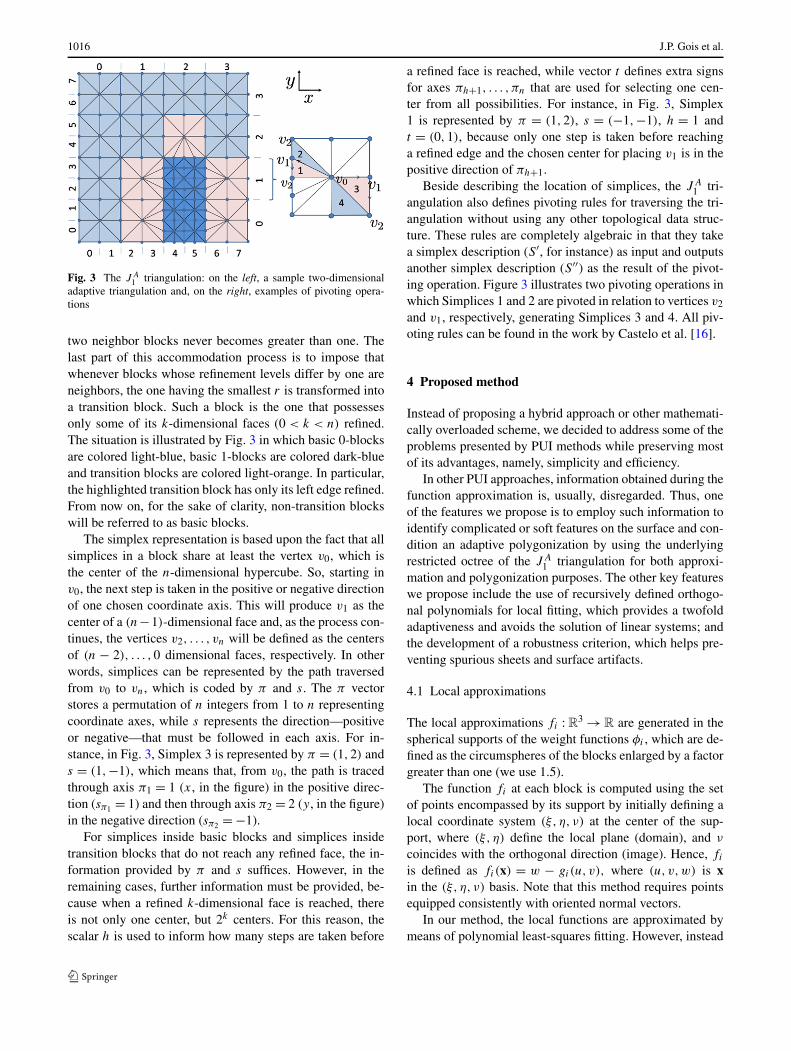
in a way that each simplex is coded by the 6-tuple S =(g, r,π, s, t, h). The first two components are related to thelocation of the block within the grid, whereas the last fouridentify the simplex within the block. Specifically, the n-dimensional vector g provides the location of a particu-lar block in a particular refinement level r . Figure 3 illus-trates, on the left, a two-dimensional JA

1 and, on the right,a highlighted block of refinement level r = 0 (0-block) andg = (3,1). Also in Fig. 3, one can find blocks with refine-ment level r = 1 (1-block) depicted in dark blue.

Before explaining how simplices are described, it is im-portant to understand that an n-dimensional JA

1 allows therefinement of an i-block by splitting it into 2n (i+1)-blocks.It is also worth to notice that, in order to accommodate thenewly created blocks, some other blocks may be forced tobe refined so that the difference in the refinement level of

1016 J.P. Gois et al.

Fig. 3 The JA1 triangulation: on the left, a sample two-dimensional

adaptive triangulation and, on the right, examples of pivoting opera-tions

two neighbor blocks never becomes greater than one. Thelast part of this accommodation process is to impose thatwhenever blocks whose refinement levels differ by one areneighbors, the one having the smallest r is transformed intoa transition block. Such a block is the one that possessesonly some of its k-dimensional faces (0 < k < n) refined.The situation is illustrated by Fig. 3 in which basic 0-blocksare colored light-blue, basic 1-blocks are colored dark-blueand transition blocks are colored light-orange. In particular,the highlighted transition block has only its left edge refined.From now on, for the sake of clarity, non-transition blockswill be referred to as basic blocks.

The simplex representation is based upon the fact that allsimplices in a block share at least the vertex v0, which isthe center of the n-dimensional hypercube. So, starting inv0, the next step is taken in the positive or negative directionof one chosen coordinate axis. This will produce v1 as thecenter of a (n−1)-dimensional face and, as the process con-tinues, the vertices v2, . . . , vn will be defined as the centersof (n − 2), . . . ,0 dimensional faces, respectively. In otherwords, simplices can be represented by the path traversedfrom v0 to vn, which is coded by π and s. The π vectorstores a permutation of n integers from 1 to n representingcoordinate axes, while s represents the direction—positiveor negative—that must be followed in each axis. For in-stance, in Fig. 3, Simplex 3 is represented by π = (1,2) ands = (1,−1), which means that, from v0, the path is tracedthrough axis π1 = 1 (x, in the figure) in the positive direc-tion (sπ1 = 1) and then through axis π2 = 2 (y, in the figure)in the negative direction (sπ2 = −1).

For simplices inside basic blocks and simplices insidetransition blocks that do not reach any refined face, the in-formation provided by π and s suffices. However, in theremaining cases, further information must be provided, be-cause when a refined k-dimensional face is reached, thereis not only one center, but 2k centers. For this reason, thescalar h is used to inform how many steps are taken before

a refined face is reached, while vector t defines extra signsfor axes πh+1, . . . , πn that are used for selecting one cen-ter from all possibilities. For instance, in Fig. 3, Simplex1 is represented by π = (1,2), s = (−1,−1), h = 1 andt = (0,1), because only one step is taken before reachinga refined edge and the chosen center for placing v1 is in thepositive direction of πh+1.

Beside describing the location of simplices, the JA1 tri-

angulation also defines pivoting rules for traversing the tri-angulation without using any other topological data struc-ture. These rules are completely algebraic in that they takea simplex description (S′, for instance) as input and outputsanother simplex description (S′′) as the result of the pivot-ing operation. Figure 3 illustrates two pivoting operations inwhich Simplices 1 and 2 are pivoted in relation to vertices v2

and v1, respectively, generating Simplices 3 and 4. All piv-oting rules can be found in the work by Castelo et al. [16].

4 Proposed method

Instead of proposing a hybrid approach or other mathemati-cally overloaded scheme, we decided to address some of theproblems presented by PUI methods while preserving mostof its advantages, namely, simplicity and efficiency.

In other PUI approaches, information obtained during thefunction approximation is, usually, disregarded. Thus, oneof the features we propose is to employ such information toidentify complicated or soft features on the surface and con-dition an adaptive polygonization by using the underlyingrestricted octree of the JA

1 triangulation for both approxi-mation and polygonization purposes. The other key featureswe propose include the use of recursively defined orthogo-nal polynomials for local fitting, which provides a twofoldadaptiveness and avoids the solution of linear systems; andthe development of a robustness criterion, which helps pre-venting spurious sheets and surface artifacts.

4.1 Local approximations

The local approximations fi : R3 → R are generated in the

spherical supports of the weight functions φi , which are de-fined as the circumspheres of the blocks enlarged by a factorgreater than one (we use 1.5).

The function fi at each block is computed using the setof points encompassed by its support by initially defining alocal coordinate system (ξ, η, ν) at the center of the sup-port, where (ξ, η) define the local plane (domain), and ν

coincides with the orthogonal direction (image). Hence, fi

is defined as fi(x) = w − gi(u, v), where (u, v,w) is xin the (ξ, η, ν) basis. Note that this method requires pointsequipped consistently with oriented normal vectors.

In our method, the local functions are approximated bymeans of polynomial least-squares fitting. However, instead

Twofold adaptive partition of unity implicits 1017

Fig. 4 Coverage domain illustration: notice that increasing the degreeof the polynomial naively may cause erroneous local solutions

of using a canonical basis {uivj : i, j ∈ N}, a basis of orthog-onal polynomials with respect to the inner product inducedby the normal equations is chosen. This way, it is not neces-sary to solve any system of equations. To find such a basis,we use the method by Bartels and Jezioranski [19]. The ad-vantages of this method, according to the authors, are thestability and the computational efficiency.

Then, given a set of orthogonal polynomials �={ψ1, . . . ,

ψl}, the polynomial fitting in local coordinates can be com-puted as:

gi(u, v) =∑

ψj ∈�

ψj (u, v)

∑mi=1 wiψj (ui, vi)

∑mi=1 ψj(ui, vi)ψj (ui, vi)

(2)

where gi is the function g subject to

ming

∑

(ui ,vi )

(g(ui, vi) − wi

)2.

The main motivation for using such orthogonal polyno-mials is their ability of generating higher-degree approxima-tions from previously computed approximations with lowadditional computational effort. This property enables thedefinition of a method that is adaptive not only in the spatialsubdivision but also in the local approximation. However,a downside of employing high-degree polynomials as localsolutions is the fact that such functions may present oscilla-tory behavior and, even if they present a small least-squareserror, they may be a poor approximation inside the region ofinterest. For instance, in Fig. 4 on the left, the polynomial isclose to the sample points inside the support, but the signsobtained when the function is evaluated in the vertices ofthe JA

1 block are not correct. Therefore, depending on theneighbor solutions, this situation may lead to extra surfacesheets or artifacts.

Before presenting a solution, one must notice that thisproblem occurs because even though high-degree polyno-mials are able to approximate point data nicely in betweenpoints, they can also oscillate at locations in which there areno points to restrain the solution, as illustrated on the leftside of Fig. 4. Based on this fact, we can observe that the

distribution of points inside the support is as important forgenerating a good function as the number of points used inthe least-squares minimization. Figures 7(c) and (d) depict areal application of the coverage domain.

Thus, we propose an approximate, but computationallyinexpensive, way to assess how well the points are distrib-uted inside the support. As in our method the local domainsare actually planes, we must determine how large is the areaof these planes covered with points. For this, we calculatethe ratio (k) between the projection of the support of theblock and the projection of the bounding box of the pointsover the plane. To that end, we create a coverage criterionfor polynomials by establishing a minimum value of k foreach polynomial degree (for instance, 0.4, 0.8 and 0.85 canbe used as the default parameters for second, third and fourthdegree polynomials). In Fig. 4 we illustrate the importanceof the coverage domain for aiding the choice of the correctfunction, since, in the example, a lower degree approxima-tion (on the right) is more suitable than a higher one (on theleft).

As mentioned before, beside the coverage criterion, wemust also take into account the minimum number of pointsthat should be used for each polynomial degree (the defaultis twice the number of polynomial bases for each degree).The union of both of these criteria constitutes the robustnesstest used in the proposed method.

An immediate issue that arises from this minimum pointtest is that not every block in the domain encloses enoughpoints for the polynomial approximation we described pre-viously. Therefore, we created a strategy for handling blockswith few or without points that differs from previous workbecause, instead of iteratively growing the support of theblock until the minimal number of points is reached [1]—which may cause a local approximation to influence a largepart of the domain—or using the approximation of the par-ent of the block [5]—which can be a poor approximation—we address this situation by searching the nearest cluster ofpoints from the current block and performing a first-degreeapproximation.

We determine such cluster of points by finding the near-est sample point r to the center of the block, by queryingenough neighbors around r (the default is 20 points), andby approximating a least-squares plane. However, depend-ing on the point distribution, the plane can be in an almostorthogonal position from the expected [20]. We detect thissituation by comparing the normal vector of the plane withthe average of the normal vectors of r neighbors. If the angleis greater than π/6, the least-squares function is substitutedby the plane with the normal vector equal to the computedaverage and the origin equals to the average neighbor posi-tion. We consider this last test as the third robustness condi-tion of the method.

Now that the most important concepts of the proposedapproach were clarified, we provide an algorithmic outline

1018 J.P. Gois et al.

of the method: after setting up the initial JA1 configuration,

for each block that does not have an approximation de-fined, the number of points inside the support of the block isqueried, originating three different situations: (i), the num-ber of points is enough for performing approximations; (ii),the number of points is not enough even for a least-squaresplane; and (iii), the number of points is greater than a speci-fied maximum threshold.

Initially, in case (i), a test that measures the variation ofpoint normal vectors from Ohtake et al. [1] is used to deter-mine the presence of two or more surface sheets inside thesame support. If they exist, the method refines the block andthe process starts again for the newly created blocks. If onlyone sheet is detected, the first-degree polynomial is calcu-lated and its degree is recursively increased until the errorcriterion is met, or until the robustness test does not allow ahigher degree or until the degree of the polynomial is equalto the maximum allowed (we use four as the default). If theprevious process finishes and error is acceptable, the approx-imation is stored in the block; otherwise, the block is refined,unless its support possesses a critical number of points (lessthan 100, in our case). In this situation, the subdivision maybe aborted if the new approximation blocks would increasethe error instead of decreasing it, due to the fact that the newblocks would enclose small amounts of points that wouldnot allow high-degree approximations.

In both parts of the above description in which the re-finement is suggested, the block may be already in the user-defined maximum allowed refinement level, so there is noother option rather than using the best approximation thatcould be calculated so far.

The approximation case (ii) is handled by searching thenearest cluster of points from the current block and perform-ing a first-degree approximation as explained above.

Finally, case (iii) is a heuristic employed to avoid use-less and expensive calculations. We consider an unnecessaryeffort to calculate minimizations for more than a thousandpoints. Thus in this case, we force subdivision of the blockwhenever the maximum refinement was not reached, other-wise the approximation is computed anyway.

We conclude this section by elucidating the differencebetween block refinements caused by approximation condi-tions and those triggered by JA

1 restrictions (explained inSect. 3.2). In the latter case, new approximations do nothave to be computed if the approximation for the block be-ing refined is already good. Figure 2 illustrates a case inwhich not all leaf nodes hold approximations associated tothem. In the figure, the blue circles represent leaf blocks thathold approximations and points inside them, the orange onesare also leaves that hold approximations despite not havingpoints in their supports, and the green one stands for a non-leaf node that holds the approximation and was only divideddue to the JA

1 accommodation process.

4.2 Function evaluation and adaptive polygonization

Given a point x inside the domain, an octree-like traversalof the JA

1 blocks is conducted to determine which blocksencompass x within their supports. The value of F (x) is ob-tained as a combination of all local functions from the sup-ports found to contain x:

F (x) =∑N

i=1 fi(x)θi(‖x − ci‖/Ri)∑N

i=1 θi(‖x − ci‖/Ri),

where N is the number of supports that affect x, fi(x), ci

and Ri are the local signed functions, center and radius ofthe block i, respectively; and, finally, the weight functionθi(t) = (1 − t2)4 that assumes zero value for t ≥ 1.

The polygonization consists first in finding an initial sim-plex, which is a straightforward task when a point near thesurface is available. Then, a traversal of all simplices thatintersect the surface through JA

1 pivoting rules is conducted,while generating the adaptive surface mesh.

4.3 Extensions to the method

The first extension concerns the addition of the sharp fea-tures capability, by properly inserting a well-known tech-nique into the originally proposed method [2].

Also, the difficulty in handling parameters in most sur-face reconstruction approaches suggests that in some casesit may be useful to allow manual edition of the function sothat the user can either fix undesirable artifact or enhance theapproximation quality by choosing more appropriated func-tions.

The last extension is related to the low quality presentedby the meshes generated by the JA

1 polygonizer. It is ac-tually a computationally inexpensive and memory efficienttechnique that displaces JA

1 vertices in order to enhance theaspect ratio of the triangles.

Examples and discussions about the use of such exten-sions are provided in Sect. 5.

Sharp features

Deciding whether or not to use sharp features at a specificregion is not a trivial problem, but the solution presented byKobbelt et al. [21] leads to nice results.

Given a set of k points P = {p1, . . . ,pk} associated withnormal vectors N = {n1, . . . ,nk}, the test consists in cal-culating the cosine of the angle between the normal vec-tor of every pair of points and checking if the minimumvalue obtained is smaller than a specified constant (0.9, asproposed by Kobbelt). If so, the region is said to containa sharp feature. For the second test, given the two points{pi ,pj } that enclose the largest angle between their normal

Twofold adaptive partition of unity implicits 1019

Fig. 5 Sharp features capability illustrated with the Filigree model(514 K points): (a) and (b) are the back and the front views in whichthe left half was generated by Ohtake’s technique and the right halfwas generated by our method

vectors {ni ,nj }, an orthogonal vector must be calculated asn∗ = ni × nj /‖ni × nj‖. After that, the maximum modu-lus of the angle cosine between n∗ and every vector in N

is calculated. If it is greater than a specified threshold (0.7),the feature is classified as a corner; otherwise, the featureis classified as an edge. In our implementation, this test iscomplemented by checking if the number of points is lowerthan a user-defined parameter (we use 30 as default).

The addition of sharp features to our technique demandedthe alteration of two parts of the algorithm explained inSect. 4.1, because the method deals differently with thecases in which a small amount of points is found in the sup-port.

In the approximation case (i), after deciding which poly-nomial gives the best fit, the sharp features test is made and,

if there is a sharp feature, an approximation for that is cal-culated [1]. If the approximation error is lower than the oneprovided by the polynomial, the sharp function is used in-stead. As for approximation case (ii), for those blocks thatoriginally presented more than zero points, we test not onlya first-degree polynomial, but also the sharp features func-tions for the point cluster. As the number of points is small inthis case, the error is not regarded, i.e., if the sharp featurestest is met, the sharp function is defined anyway.

Interactive implicit function editing

For the function editing feature, we exploit one of the advan-tages presented by PUI methods over other techniques suchas moving least-squares (MLS) or RBF; namely, the fact thatthe global function is defined by a set of independent localfunctions in subdomains, i.e., changing one of these func-tions only affects the global function locally. Thus, changinglocal traits of the function consists in locating the desiredblock and switching the associated approximation. Findingsuch a block on the JA

1 triangulation in quite straightfor-ward, since its structure consists of a restricted octree. Thecalculation is made by testing the blocks that contain the de-sired point, in different refinement levels, until the one withthe function is found.

In our implementation, we developed a graphic toolfor choosing points over a reconstructed model and se-lecting a new function from the following options: con-stant function—that can be user-defined or calculated auto-matically—polynomials and sharp features functions.

Mesh enhancement

We choose the mesh displacement technique because it isquite simple to implement and does not impose a heavy bur-den on the time and memory complexities of the polygo-nizer. However, as the degrees of freedom for moving JA

1vertices without invalidating the structure are constrained,the improvement is limited. The idea is to move the verticesaway from the surface, in an inversely proportional measurein relation to the function value, in order to improve the as-pect ratio of the mesh elements.

We apply the displacements only on vertices belonging tosimplices that intersect the surface during the polygoniza-tion. For that reason, no extra memory is required and theextra computational effort is due to the calculation of an ap-proximation for the maximum value of the function and forevaluating the gradient of the function in every displacedvertex. The following equation presents how a vertex x istaken to its new position xnew:

xnew = x+[

sign(F (x))

‖∇F ‖( |Fmax| − |F (x)|

|Fmax|)2

e(l)

4α

]

∇F (x)

1020 J.P. Gois et al.

Fig. 6 Illustration of the deformation of a JA1 block: the vertex dis-

placement technique is able to create more uniform mesh elements

where sign(F (x)) represents the function sign, Fmax is anestimative to the maximum of the function in the domain, l isthe refinement level associated to the vertex, e(l) is the sizeof a JA

1 block edge in the refinement level l, and 0 < α < 1determines the maximum amplitude of the movement.

For basic blocks, the refinement level associated with avertex l is equal to the refinement of the block r ; whereas,for transition blocks, it is equal to (r + 1) for vertices thatlie in refined faces and equal to r for the remaining ones. Itis worth to mention that e(l)/4 is the maximum amplitudeof the displacement—in any direction—allowed by the JA

1structure.

In Fig. 6 a representation of the displacement of the ver-tices is depicted in two dimensions.

5 Results and discussion

In Fig. 7, we illustrate the importance of the coverage do-main, as well as the interactive function editing procedure.In (a), the 362 K raw data Stanford Bunny was reconstructedusing the method by Ohtake et al. [1] using its default para-meters, but without sharp features, while in (b), we selectedthe parameters to match those used with our method (max-imum refinement as 9 and error threshold as 0.002), againwithout sharp features, since their use generated even moreartifacts. In (c), we used our technique to reconstruct thesame model without the coverage criterion. One can noticethe presence of several artifacts on the surface and some ex-tra sheets, that were almost eliminated with the use of thecoverage test (Fig. 7(d)). In Fig. 7(e), we defined a selectionof blocks, for which a constant function was set with posi-tive values (0.002), in order to eliminate some of the surfaceflaws. Finally, Fig. 7(f) depicts the bunny after the functionediting.

The models reconstructed using the Ohtake et al. tech-nique presented a series of extra sheets and surface artifactsfor both versions. In the work by Kazhdan et al. [10], similarproblems were presented for the Ohtake’s method. Never-theless, the differences are the fact that sharp features wereused and the employed polygonization technique which gen-erated the mesh for only one connected component. The lat-ter was responsible for hiding most of the spurious sheets.

Fig. 7 Function edition: (a)–(b) The Ohtake et al. method with itsdefault parameters and with suggested parameters; (c) reconstructionusing the proposed method without coverage domain; (d) reconstruc-tion with coverage domain; (e) user selected imperfections; (f) func-tion changed in order to eliminate imperfections. Comparisons againstother surface reconstructions can be found in [10]

The situation, illustrated by Fig. 7, shows that the set ofsolutions proposed in this paper considerably enhance therobustness of the reconstructions, given the fact that, evenwithout the coverage criterion and in the presence of noise,the method was able to minimize the number of defects.

Also concerning function editing, we present, in Fig. 8,another example in which plane functions, employed duean user-defined configuration (Fig. 8(b)), were replaced bysecond-degree polynomials. Differently from the previousexample, in this one we used the edition to enhance the qual-ity of the function and not to remove defects. The compari-son between Figs. 8(a) and (c) illustrates the quality gain.

Twofold adaptive partition of unity implicits 1021

Fig. 8 Enhancing the modelusing function editing: (a) amodel without high-orderapproximations (due toconfiguration), (b) selectedblocks for function changing,and (c) the final result

The next test we conducted demonstrates the ability ofrepresenting sharp features. In Fig. 5, there is a comparisonbetween our method (right half of the figure) and the methodfrom Ohtake et al. [1] (left half of the figure) using similarparameters for the error threshold and for maximum depth.One can notice that the former was able to generate a slightlybetter and more robust function, but at a slightly more ex-pensive computation. While the Ohtake’s method generatedthe 1280×1024 ray-traced viewport in 1527 s for the frontalview, ours took 1620 s to perform the same task. One ma-jor difference between the methods is that, in our approach,the evaluation is decoupled from the function approxima-tion, in the sense that the whole function is built before thefirst evaluation is made. This fact means that for coarse gridsor small ray-tracer viewports, the Ohtake’s method tends tobe faster, but as soon as the number of required functionevaluations increases, the methods are similar in terms ofprocessing time.

Another substantial difference between the methods isthe function behavior in regions away from the zero-set. Theproposed method presents a bounded maximum gradientmagnitude for the whole domain due to all robustness cri-teria applied during the approximation phase. For instance,for the models presented in Fig. 5, the ray-tracer algorithmwe employed [22] accused a maximum gradient magnitudeof 1.9 for our method and of 1010 for the other one.

In order to illustrate the mesh displacement technique, wereconstructed the Chinese dragon model (665 K points) us-ing maximum refinement level 7 without sharp features. Fig-ure 9 shows, on the left, the original mesh and, on the right,the model generated with mesh displacement. Both meshesare composed of 535,605 triangles and the time taken forpolygonizing the models was 39.433 s and 202.9 s for thenormal and the displaced JA

1 version, respectively. Thisslow-down was expected for the displaced version, since itrequires more evaluations of the function to compute the ap-proximation for the gradient, but even so, this extra cost isconstant and does not affect the complexity of the algorithm.

To assess the improvement of the triangles caused bythe displacement, we use the aspect ratio measure α� =√

3emaxP12A

, where emax is the largest edge, P is the perimeter

Fig. 9 Comparing the original iso-mesh produced purely by JA1 (top)

against the iso-mesh obtained from JA1 with displacement (bottom)

and A is the area of the triangle. Notice that the best aspectratio is 1.0 (equilateral triangle).

For the normal mesh, the average aspect ratio was 5.55and the standard deviation was 128.09, whereas for the en-hanced mesh, the average was 1.68 and the standard devia-tion was 0.61. This result confirms the effectiveness of the

1022 J.P. Gois et al.

Fig. 10 A CSG difference operation involving the Neptune model anda cylinder

technique because it enabled not only to enhance the averagequality of the triangles but also to decrease the variation ofthe aspect ratio, which means that the whole mesh presentsa reasonable overall aspect ratio.

As for the memory peak, for the Neptune model (2 Mpoints) the function generation reached 660 MB. When JA

1polygonization is taken into account, the peak was 850 MB.Finally, in Fig. 10, we demonstrate a CSG difference opera-tion between the Neptune model and a cylinder.

6 Conclusion

We presented a twofold adaptive method in the sense thatit is not only adaptive in the domain refinement, but alsoin the degrees of the local approximations that are calcu-lated in an efficient and robust way. The robustness of themethod is achieved through several enhancements concern-ing the problems that arise in other PUI techniques. Also,the JA

1 triangulation was employed to gather informationfrom the function approximation and to use it to performan adaptive polygonization. We also presented extensions toour method, including sharp features, the interactive editingof the implicit function and the mesh enhancement.

The results demonstrate that the method is able to achievemore robustness and also that the computational cost is com-parable to others when the number of function evaluations isconsiderable.

As future works, we intend to derive theoretical war-ranties concerning the use of the coverage domain to assure

function quality and also to further explore the function edit-ing feature.

Acknowledgements This work was partially supported by DAAD,with grants number A/04/08711 and FAPESP, with grants number04/10947-6, 05/57735-6 and 06/54477-9. The authors also thank JoãoComba and Carlos Dietrich for the comments on mesh displacements.The models were obtained from Aim@Shape Project–Shape Reposi-tory and The Stanford 3D Scanning Repository.

References

1. Ohtake, Y., Belyaev, A., Alexa, M., Turk, G., Seidel, H.P.: Multi-level partition of unity implicits. ACM Trans. Graph. 22(3), 463–470 (2003)

2. Gois, J.P., Polizelli-Junior, V., Etiene, T., Tejada, E., Castelo, A.,Ertl, T., Nonato, L.G.: Robust and adaptive surface reconstruc-tion using partition of unity implicits. In: Brazilian Symposiumon Computer Graphics and Image Processing, pp. 95–102 (2007)

3. Bloomenthal, J.: An implicit surface polygonizer. In: Graph-ics Gems IV, pp. 324–349. Academic Press, San Diego (1994).citeseer.ist.psu.edu/bloomenthal94implicit.html

4. Ohtake, Y., Belyaev, A., Seidel, H.P.: Sparse surface reconstruc-tion with adaptive partition of unity and radial basis functions.Graph. Models 68(1), 15–24 (2006)

5. Mederos, B., Arouca, S., Lage, M., Lopes, H., Velho, L.: Improvedpartition of unity implicit surface reconstruction. Technical ReportTR-0406, IMPA, Brazil (2006)

6. Chen, Y.L., Lai, S.H.: A partition-of-unity based algorithm for im-plicit surface reconstruction using belief propagation. In: IEEE In-ternational Conference on Shape Modeling and Applications, pp.147–155 (2007)

7. Xia, Q., Wang, M.Y., Wu, X.: Orthogonal least squares in partitionof unity surface reconstruction with radial basis function. In: Con-ference on Geometric Modeling and Imaging, pp. 28–33 (2006)

8. Tobor, I., Reuter, P., Schlick, C.: Reconstructing multi-scale vari-ational partition of unity implicit surfaces with attributes. Graph.Models 68(1), 25–41 (2006)

9. Kazhdan, M.: Reconstruction of solid models from oriented pointsets. In: Eurographics Symposium on Geometry Processing, pp.73–82 (2005)

10. Kazhdan, M., Bolitho, M., Hoppe, H.: Poisson surface reconstruc-tion. In: Eurographics Symposium on Geometry Processing, pp.61–70 (2006)

11. Bolitho, M., Kazhdan, M., Burns, R., Hoppe, H.: Multilevelstreaming for out-of-core surface reconstruction. In: Eurograph-ics Symposium on Geometry Processing, pp. 69–78 (2007)

12. Bloomenthal, J.: Polygonization of implicit surfaces. Comput.Aided Geom. Des. 5(4), 341–355 (1988)

13. Hall, M., Warren, J.: Adaptive polygonalization of implicitly de-fined surfaces. IEEE Comput. Graph. Appl. 10(6), 33–42 (1990)

14. Paiva, A., Lopes, H., Lewiner, T., de Figueiredo, L.H.: Robustadaptive meshes for implicit surfaces. In: Brazilian Symposium onComputer Graphics and Image Processing, pp. 205–212 (2006)

15. Kazhdan, M., Klein, A., Dalal, K., Hoppe, H.: Unconstrained iso-surface extraction on arbitrary octrees. In: Eurographics Sympo-sium on Geometry Processing, pp. 125–133 (2007)

16. Castelo, A., Nonato, L.G., Siqueira, M., Minghim, R., Tavares, G.:The j1a triangulation: An adaptive triangulation in any dimension.Comput. Graph. 30(5), 737–753 (2006)

17. de Figueiredo, L.H., Gomes, J.M., Terzopoulos, D., Velho, L.:Physically-based methods for polygonization of implicit surfaces.In: Conference on Graphics Interface, pp. 250–257 (1992)

Twofold adaptive partition of unity implicits 1023

18. Schreiner, J., Scheidegger, C., Silva, C.: High-quality extractionof isosurfaces from regular and irregular grids. IEEE Trans. Vis.Comput. Graph. 12(5), 1205–1212 (2006)

19. Bartels, R.H., Jezioranski, J.J.: Least-squares fitting using orthog-onal multinomials. ACM Trans. Math. Softw. 11(3), 201–217(1985)

20. Amenta, N., Kil, Y.J.: The domain of a point set surfaces. Euro-graphics Symp. Point-based Graph. 1(1), 139–147 (2004)

21. Kobbelt, L.P., Botsch, M., Schwanecke, U., Seidel, H.P.: Featuresensitive surface extraction from volume data. In: SIGGRAPH’01,pp. 57–66 (2001)

22. PovRay: Persistence of vision. http://www.porvay.org (2007)

J.P. Gois is a PhD candidate inComputational Mathematics at In-stitute for Mathematics and Com-puter Science–University of SãoPaulo, Brazil (ICMC-USP). He re-ceived a MSc degree in Computa-tional Mathematics at ICMC-USPin 2004 and a Mathematics degreeat State University of São Paulo,Brazil (UNESP) in 2002. He alsowas invited researcher at Universityof Stuttgart, Germany. His researchinterests are Surface Reconstruc-tion, Mesh Generation and Compu-tational Mathematics.

V. Polizelli-Junior is a MSc candi-date in Computer Science at ICMC-USP. He also holds a BSc degreein Computer Science from UNESP.His research interest is IsosurfaceExtraction Methods and GeometricModeling.

T. Etiene is a MSc candidate inComputer Science at ICMC-USP.He also holds a BSc degree in Com-puter Science from ICMC-USP. Hisresearch interests are Fluid FlowSimulation for Computer GraphicsApplications and Interactive Meth-ods for Computer Graphics.

E. Tejada is a PhD candidate atthe Visualization and InteractiveSystems Institute of the Univer-sity of Stuttgart. He holds a MScon Computer Science from ICMC-USP. His research interests includepoint-based graphics, visualizationand hardware-accelerated graphics.

A. Castelo received the PhD de-gree in mathematics from PontificalCatholic University–Rio de Janeiro(PUC-RIO), Brazil, in 1992. Since1992, he has been an Assistant Pro-fessor at ICMC-USP. His major re-search interests are ComputationalGeometry, Computational Topol-ogy, and Computational Fluid Dy-namics.

L.G. Nonato received his PhD atPUC-RIO in 1998. He has been re-searcher at University of São Paulosince 1999 and is currently an As-sistant Professor. His research inter-ests involve Computational Geome-try, Computer Graphics and Compu-tational Topology.

T. Ertl received a PhD in theoret-ical astrophysics from the Univer-sity of Tuebingen, Germany. Cur-rently, Dr. Ertl is a full professor ofcomputer science at the Universityof Stuttgart and the head of the Vi-sualization and Interactive SystemsInstitute (VIS). His research inter-ests include visualization, computergraphics and human–computer in-teraction. Dr. Ertl served on sev-eral programs and paper commit-tees, as well as a reviewer for nu-merous conferences and journals inthe field.