Chapter 7 Linear Programming - HCC Learning Web

Lecture Note

7.1 Graphing Linear Inequalities in Two Variables

7.2 Linear Programming: The Graphical Method

7.3 Applications of Linear Programming

7.4 The Simplex Method: Programming

7.5 Maximization Applications

7.6 The Simplex Method: Duality and Minimization

7.7 The Simplex Method: Nonstandard Problems

Chapter 7 Linear Programming

Lecture Note

Linear Inequality in Two Variables: A linear inequality in two variables is aninequality in the form of𝑨𝒙 + 𝑩𝒚 ≥ 𝑪, 𝑨𝒙 + 𝑩𝒚 > 𝑪, 𝑨𝒙 + 𝑩𝒚 ≤ 𝑪, 𝐨𝐫 𝑨𝒙 + 𝑩𝒚 < 𝑪

(𝑎, 𝑏, and 𝑐 are constants, and 𝑥 and 𝑦 are variables.)

A solution of a linear inequality is an ordered pair that satisfies the inequality. Alinear inequality has infinite number of solutions, one for every choice of a valuefor 𝑥. The best way to show these solutions is to sketch the graph of theinequality, which consists of all points in the plane whose coordinates satisfy theinequality.

Chapter 7.1 Graphing Linear Inequalities in Two Variables

Lecture Note

Graphing of the Inequality in Two Variables

Step 1: Rewrite the inequality in the form of𝒚 ≥ 𝒎𝒙+ 𝒃, 𝒚 > 𝒎𝒙+ 𝒃, 𝒚 ≤ 𝒎𝒙+ 𝒃, 𝐨𝐫 𝒚 < 𝒎𝒙+ 𝒃

Step 2: Sketch the graph of 𝑦 = 𝑚𝑥 + 𝑏 (the boundary line). This line willseparate the plane into two parts, solution part and nonsolution part.

Step 3: Use a test point to determine which side is a solution side. In a singleinequality use the following:


Inequality Solution Consists of All Points

𝑦 ≥ 𝑚𝑥 + 𝑏 on or above the line 𝑦 = 𝑚𝑥 + 𝑏

𝑦 > 𝑚𝑥 + 𝑏 above the line 𝑦 = 𝑚𝑥 + 𝑏

𝑦 ≤ 𝑚𝑥 + 𝑏 on or below the line 𝑦 = 𝑚𝑥 + 𝑏

𝑦 < 𝑚𝑥 + 𝑏 below the line 𝑦 = 𝑚𝑥 + 𝑏

Lecture Note

Example 1-3. Graph each inequality(a) 3𝑥 − 2𝑦 ≤ 6 (b) 𝑥 + 4𝑦 < 4 (c) 5𝑦 − 2𝑥 ≤ 10


Example 4. Graph each inequality(a) 𝑦 ≥ 2 (b) 𝑥 ≤ −1

Lecture Note

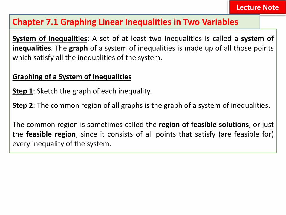
System of Inequalities: A set of at least two inequalities is called a system ofinequalities. The graph of a system of inequalities is made up of all those pointswhich satisfy all the inequalities of the system.

Graphing of a System of Inequalities

Step 1: Sketch the graph of each inequality.

Step 2: The common region of all graphs is the graph of a system of inequalities.

The common region is sometimes called the region of feasible solutions, or justthe feasible region, since it consists of all points that satisfy (are feasible for)every inequality of the system.


Lecture Note

Example 6. Graph each system

3𝑥 + 𝑦 ≤ 12

𝑥 ≤ 2𝑦


Lecture Note

Example 7. Graph the feasible region for the system

2𝑥 − 5𝑦 ≤ 10𝑥 + 2𝑦 ≤ 8𝑥 ≥ 0, 𝑦 ≥ 0


Lecture Note

Example 8. Graph the feasible region for the system

5𝑦 − 2𝑥 ≤ 10𝑥 ≥ 3, 𝑦 ≥ 2


Lecture Note

Example 9. In 2017, the T. Rowe Price Tax-Free High-Yield Fund paid a 3-yearreturn of 5%, and the BlackRock California Municipal Opportunities Fund paid a3-year return of 4%. Sherri would like to invest up to $75,000 and obtain at least$2500 in invest over the 3-year period. Write a system of inequalities expressingthese conditions and graph the feasible region.(Data from: 222.morningstar.com.)


Lecture Note

Optimization Problems: Many problems in business, science, and economicsinvolve finding the optimal value of function (for instance, the maximum value ofthe profit function or the minimum value of the cost function), subject to variousconstraints (such as transportation costs, environmental protection laws,availability of parts, and interest rates)

Linear programming deals with such situations. In linear programming, thefunction to be optimized, called the objective function, is linear and theconstraints are given by linear inequalities. Linear programming problems thatinvolve only two variables can be solved by the graphical method.

Chapter 7.2 Linear Programming: The Graphical Method

Lecture Note

Solving Linear Programming Problems:

Graph the feasible reason for constraints, then move the graph of the objectivefunction to determine where the function makes the maximum or minimum.A point in the feasible region where the boundary lines of two constraints crossis called a corner point.

When the feasible region is enclosed by boundary lines on all sides, the region isbounded. Otherwise, the region is unbounded. Liner programming problemswith bounded regions always have solutions. If the feasible region is unbounded,linear programming problems may not have maximum or minimum.


Lecture Note


Example 1. Find the maximum and minimum values of the objective function𝑧 = 2𝑥 + 5y, subject to the following constraints

3𝑥 + 2𝑦 ≤ 6−2𝑥 + 4𝑦 ≤ 8

𝑥 + 𝑦 ≥ 1𝑥 ≥ 0, 𝑦 ≥ 0

Lecture Note

Corner Point Theorem:

If the feasible region is bounded, then the objective function has both amaximum and a minimum value, and each occurs at one or more corner points.

If the feasible region is unbounded, the objective function may not have amaximum or minimum. But if a maximum or minimum value exists, it will occurat one or more corner points.


Lecture Note

Solving a Linear Programming Problem Graphically:

1. Write the objective function and all necessary constraints.2. Graph the feasible regions.3. Determine the coordinates of each of the corner points.4. Find the value of the objective function at each corner point.5. If the feasible region is bounded, the solution is given by the corner point

producing the optimum value of the objective function.6. If the feasible region is an unbounded region in the first quadrant and both

coefficients of the objection function are positive, then the minimum valueof the objective function occurs at a corner point and there is no maximumvalue.


Lecture Note


Example 2. Sketch the feasible region for the following set of constraints:

3𝑦 − 2𝑥 ≥ 0𝑦 + 8𝑥 ≤ 52𝑦 − 2𝑥 ≤ 2

𝑥 ≥ 3

Then find the maximum and minimum values of the objective function 𝑧 = 5𝑥 +2𝑦.

Lecture Note


Example 3. Solve the following linear programming problem.Minimize 𝑧 = 𝑥 + 3𝑦

subject to

2𝑥 + 𝑦 ≤ 105𝑥 + 2𝑦 ≥ 20−𝑥 + 2𝑦 ≥ 0𝑥 ≥ 0, 𝑦 ≥ 0

Lecture Note


Example 4. Solve the following linear programming problem.Minimize 𝑧 = 2𝑥 + 4𝑦

subject to

𝑥 + 2𝑦 ≥ 103𝑥 + 𝑦 ≥ 10𝑥 ≥ 0, 𝑦 ≥ 0

Lecture Note

Example 1: An office manager needs to purchase new filing cabinets. He knowsthat Ace cabinets cost $40 each, requires 6 square feet of floor space, and hold 8cubic feet of files. On the other hand, each Excello cabinet costs $80, requires 8square feet of floor space, and holds 12 cubic feet. His budget permits him tospend no more than $560, while the office has room for no more than 72 squarefeet of cabinets. The manager desires the greatest storage capacity within thelimitations imposed by funds and space. How many each type of cabinet shouldhe buy?

Chapter 7.3 Applications of Linear Programming

Lecture Note

Example 2: Certain laboratory animals must have at least 30 grams of proteinand at least 20 grams of fat per feeding period. These nutrients come from food𝐴, which costs 18 cents per unit and supplies 2 grams of protein and 4 of fat, andfood 𝐵, with 6 grams of protein and 2 of fat, costing 12 cents per unit. Food 𝐵 isbought under a long-term contract requiring that at least 2 units of 𝐵 be usedper serving. How much of each food must be bought to produce the minimumcost per serving?


Lecture Note

Example 3: Mariana wants to invest up to $5000 in stocks. The share price forCVS Health Corp. is $81 and the share price for Target Corp. is $57. Based on theaverage of 10-year returns, CVS would produce in a year a profit of $11 pershare, and Target would produce a profit of $4 per share. Mariana would like toobtain at least $520 in profit. A measure of risk for each of these stocks is thebeta value. The lower the beta value, the less risk associated with that stock. Ifthe beta value for CVS is .62 and the beta value for Target is .24, how manyshares of each stock should Mariana purchase to minimize the risk as measuredby the beta value? (Data from: www.Morningstar.com.)


Lecture Nott. e

Simplex method is a method of solving linear programming problems with manyvariables using matrix. Because the simplex method is used for problems withmany variables, it usually is not convenient to use letters such as 𝑥, 𝑦, 𝑧, or 𝑤 asvariable names. Instead, the symbols 𝑥1(read “𝑥-sub-one”), 𝑥2, 𝑥3, and so on, upto 𝑥𝑛, are used. In the simplex method, all constraints must be expressed in thelinear form

𝑎1𝑥1 + 𝑎2𝑥2 + 𝑎3𝑥3 +⋯+ 𝑎𝑛𝑥𝑛 ≤ 𝑏,where 𝑥1, 𝑥2, 𝑥3, ⋯ , 𝑥𝑛 are variables, 𝑎1, 𝑎2, 𝑎3, ⋯ , 𝑎𝑛 are coefficients, and 𝑏 is aconstant.

Chapter 7.4 The Simplex Method: Maximization

Lecture Nott. e

Standard Maximum Form

A linear programming problem is in standard maximum form if1. the objective function is to be maximized;2. all variables are nonnegative (𝑥𝑖 ≥ 0, 𝑖 = 1, 2, 3,⋯ );3. all constraints involve ≤;4. the constants on the right side in the constraints are all nonnegative (𝑏 ≥ 0)


Lecture Nott. e


Setting up the Problem

Convert each constraint, a linear inequality, into a linear equation. This is doneby adding a nonnegative variable, called a slack variable, to each constraint. Forexample, convert the inequality 𝑥1 + 𝑥2 ≤ 10 into an equation by adding theslack variable 𝑠1, to get

𝑥1 + 𝑥2 + 𝑠1 = 0, where 𝑠1 ≥ 0.

Selecting the Pivot

In the Gauss-Jordan method a particular nonzero entry in the matrix is chosenand changed to a 1; then all other entries in that column are changed to zeros. Asimilar process is used in the simplex method. The chosen entry is called thepivot. In choosing the pivot, we choose the pivot column which is the columncontaining the most negative indicator. Then for each positive entry in the pivotcolumn, divide the number in the far right column of the same row by thepositive number in the pivot column. The row with the smallest quotient iscalled the pivot row. The entry in the pivot row and pivot column is the pivot.

Lecture Nott. e


Pivoting

Once the pivot has been selected, row operation s are used to replace the initialsimplex tableau by another simplex tableau in which the pivot column variable iseliminated from all but one of the equations. Since this new tableau is obtainedby row operations, it represents an equivalent system of equations (that is, asystem with the same solutions as the original system). This process is calledpivoting.

Repeat the Process

When at least one of the indicators in the last row of a simplex tableau isnegative, the simplex method requires that a new pivot be selected and thepivoting be performed again. This procedure is repeated until a simplex tableauwith no negative indicators in the last row is obtained or a tableau is reached inwhich no pivot row can be chosen.

Lecture Nott. e


Repeat the Process

When at least one of the indicators in the last row of a simplex tableau isnegative, the simplex method requires that a new pivot be selected and thepivoting be performed again. This procedure is repeated until a simplex tableauwith no negative indicators in the last row is obtained or a tableau is reached inwhich no pivot row can be chosen.

Read the Solution with the Final Simplex Tableau

When there are no negative indicators in the last row, no further pivoting isnecessary, and we call this the final simplex tableau. Once the final simplextableau is obtained, read the solution

Lecture Nott. e


Basic Variables and Nonbasic variables

In any simplex tableau, some columns look like columns of an identity matrix(one entry is 1 and the rest are 0). The variables corresponding to these columnsare called basic variables and the variables corresponding to the other columnsare referred to as nonbasic variables.

Lecture Nott. e


Simplex Method

1. Determine the objective function.2. Write down all necessary constraints.3. Convert each constraint into an equation by adding a slack variable.4. Set up the initial simplex tableau.5. Locate the most negative indicator. If there are two such indicators, choose one. The indicator

determines the pivot column.6. Use the positive entries in the pivot column to form the quotients necessary for determining

the pivot. If there are no positive entries in the pivot column, no maximum solution exists. Iftwo quotients are equally the smallest, let either determines the pivot.

7. Multiply every entry in the pivot row by the reciprocal of the pivot to change the pivot to 1.Then use row operations to change all other entries in the pivot column to 0 by adding suitablemultiples of the pivot row to the other rows.

8. If the indicators are all positive or 0, you have found the final tableau. If not, go back to Step 5and repeat the process until a tableau with no negative indicators is obtained.

9. In the final tableau, the basic variables correspond to the columns that have one entry of 1 andthe rest 0. The nonbasic variables correspond to the other columns. Set each nonbasic variablesequal to 0 and solve the system for the basic variables. The maximum value of the objectivefunction is the number in the lower right-hand corner of the final tableau.

Lecture Note

Example 1. Solve the following linear programming problem.Maximize 𝑧 = 2𝑥1 + 3𝑥2 + 𝑥3

subject to

𝑥1+𝑥2 + 4𝑥3 ≤ 100𝑥1+2𝑥2 + 𝑥3 ≤ 150

3𝑥1 + 2𝑥2 + 𝑥3 ≤ 320𝑥1 ≥ 0, 𝑥2 ≥ 0, 𝑥3 ≥ 0


Lecture Note

Example 6. Solve the following linear programming problem using the simplexmthod.

Maximize 𝑧 = 8𝑥1 + 12𝑥2

subject to 40𝑥1 + 80𝑥2 ≤ 5606𝑥1 + 8𝑥2 ≤ 72𝑥1 ≥ 0, 𝑥2 ≥ 0


Lecture Nott. e

Example 1 A farmer has 110 acres of available land he wishes to plant with amixture of potatoes, corn, and cabbage. If costs him $400 to produce an acre ofpotatoes, $160 to produce an acre of corn, and $280 to produce an acre ofcabbage. He has a maximum of $20,000 to spend. He makes a profit of $120 peracre of potatoes, $40 per acre of corn, and $60 per acre of cabbage.

Chapter 7.5 Maximization Applications

Lecture Nott. e

Example 2 Ana Pott, who is a candidate for the state legislature, hs $96,000 tobuy TV advertising time. Ads cost $400 per minute on a local cable channel,$4000 per minute on a regional independent channel, and $12,000 per minuteon a national network channel. Because of existing contracts, the TV stations canprovide at most a total of 30 minutes of advertising time, with a maximum of 6minutes on the national network channel. At any given time during the evening,approximately 100,000 people watch the cable channel. 200,000 theindependent channel, and 600,000 the network channel. To get maximumexposure, how much time should Ana buy from each station?(a) Set up the initial simplex tableau for this problem.(b) Use the simplex method to find the final simplex tableau.(c) What do the values of the slack variables in the optimal solution tell you?


Lecture Nott. e

Example 3 A chemical plant makes three products – glaze, solvent, and clay –each of which brings in different revenue per truck load. Production is limited,first by the number of air pollution units the plant is allowed to produce eachday and second by the time available in the evaporation tank. The plant managerwants to maximize the daily revenue. Using information not given here, he setsup an initial simplex tableau and uses the simplex method to produce thefollowing final simplex tableau:

𝑥1 𝑥2 𝑥3 𝑠1 𝑠2−10 −25 0 1 − 1 60

3 4 1 0 .1 247 13 0 0 .4 96

The three variables represent the number of truckloads of glaze, solvent, andclay, respectively. The first slack variable comes from the air pollution constraintand the second slack variable from the time constraint on the evaporation tank.The revenue function is given in hundreds of dollars.(a) What is the optimal solution?(b) Interpret this solution. What do the variables represent, and what does the

solution mean?


Chapter 7 Linear Programming - HCC Learning Web

Documents

Transcript of Chapter 7 Linear Programming - HCC Learning Web