1

SOR1311 LINEAR PROGRAMMING

Lecturers: Ms. Natalie Attard, Dr. Jaroslav Sklenar

Credits: 2

Prerequisites: Pure or Applied Mathematics at the level requested for entry to engineering and technology courses

Lectures: 1 hour per week for 14 hours + tutorials and computer lab

sessions

Course held during: Semester 2

CONTENT

� Problem formulation

� Simplex Method

� Duality

� Sensitivity Analysis

� Network Problems (Transportation and Assignment) � Integer Linear Programming

� Modelling and LP Software Packages

The emphasis during this study unit will be on the practical aspects of the linear programming problem. More time will be dedicated to problem formulation and

numerical solution rather than the mathematical background.

Method of Assessment: Test

Suggested Texts:

1. Bazaraa, M.S., Jarvis, J.J. and Sherali, H.D. ( 1990 ) Linear Programming and

Network Flows, John Wiley & Sons. 2. Ahuja, R.K., Magnanti, T.L., Orlin, J.B. ( 1993 ) Network Flows - Theory,

Algorithms, and Applications, Prentice-Hall.

3. Nemhauser, G.L., Wolsey,L.A. ( 1999 ) Integer and Combinatorial Optimization,

John Wiley & Sons. 4. Williams, H.P. ( 1999 ) Model Building in Mathematical Programming, John

Wiley & Sons.

5. Lucey, T. ( 1996 ) Quantitative Techniques, DP Publications.

6. Lofti, V., Pegels, C.C ( 1996 ) Decision Support Systems for Operations

Management and Management Science, IRWIN. 7. Eppen, G.D., Gould, F.J. and Schmidt, C.P. ( 1996 ) Introductory Management

Science, Prentice-Hall.

2

Chapter 1: Introduction to Mathematical Programming

Mathematical programming refers to a set of procedures which deal with the analysis

of optimization problems. Optimization problems are generally those in which a

decision maker wishes to optimize some measure(s) of satisfactions by selecting

values for a set of variables. Thus, a mathematical programming model answers the

question “What’s best?” rather than “What happened?” or “What if?” or “What will happen?” or “Why it happened?”

Before moving on, it is important to point out that the word "programming" has nothing to do with “computer programming”. A “program” here is referred to a

“decision program”, that is, a strategy or a rule. In fact, the term "mathematical

programming" was coined before the word "programming" became closely

associated with computer software. The origin of the term “programming” in this

context comes from the fact that the technique of linear programming (see later) has been used for the first time for optimization of military training programmes.

A number of applications have been translated into mathematical programming

terms. The following is a typical example:

Suppose a furniture company manufactures four models of desks. Each desk is first

constructed in the carpentry shop, then is sent to the finishing shop, where it is

varnished, waxed and polished. The number of labor-hours required in each shop

and the number of hours available in each shop are known. The company wants to determine the quantities to make of each type of desk in order to maximize profit.

In other words an optimization problem is essentially about finding the best solution

to a given problem from a set of feasible solutions. It consists of three components:

1. a solution (decision) vector, that is, how can we achieve an optimal objective

(how much do we need to produce of each type of desk)?

2. the objective or objectives, that is, what do we want to optimize (maximize

profit in the above example)?

3. the set of all feasible solutions, that is, among which possible options may we

choose to optimize (constraints – labor hours)?

Mathematically an optimization problem is one in which the value of a given

function : nf →� � is to be maximized or minimized over a given set nS ⊆ � . The

function f is called the objective function, and the set S the constraint set or

feasible set. The following notation will be used:

3

max{ ( ) }f S∈x

x x

or

min{ ( ) }f S∈x

x x

A solution to the above problems is a vector x called the vector of decision

variables.

When the constraint set nS = � , the optimization problem is referred to as

“unconstrained optimization”. In other words, unconstrained optimization deals with

the maximization/minimization of a function without any restrictions. On the other

hand, when nS ⊂ � , the problem is referred to as “constrained optimization”.

Example

Suppose that on a particular island, there are two power stations A and B. Suppose

that at a particular time of the day, the demand for electricity amounts to 2

megawatts (MW). Let us denote by x the amount of electricity generated by A,

which implies that the remaining amount of electricity generated by B must be 2-x.

There are various ways in which the demand can be met. For example the Electricity

Company can produce x=2 so that A produces all the power or x=0, so that B

produces all the power, or x to have some other value, so that both A and B

contribute.

Suppose that the cost CB of running power station B is proportional to its output i.e.

2BC x= − , and the cost CA of running power station A in relation to the amount of

electricity generated is: 2

2 2A

x xC = + . Adding these two cost functions yields:

2

( ) 22 2

A B

x xC C f x+ = = − +

The Company wants to find that value of x for which this total cost is minimized.

Since there are no specified restrictions, this unconstrained optimization problem can

be solved by applying the differential calculus:

2

min min

. . ( ) 2 02 2

0.5 , ( ) 1.875

A B

x xi e C C

x x

x MW f x

∂ ∂+ = − + = ∂ ∂

⇒ = =

The following figure shows the graph of the cost function f(x).

4

-5 -4 -3 -2 -1 0 1 2 3 4 50

2

4

6

8

10

12

14

16

18

Examples of other applications

• Airline companies schedule crews and aircraft to minimize their costs

• Investors create portfolios to avoid the risks and achieve the maximum profits

• Manufacturers minimize the production costs and maximize the efficiency

• Bidders optimize their bidding strategies to achieve best results

• Physical system tends to a state of minimum energy

Various types of mathematical programming problems

Mathematical programming encompasses many different types of problems:

1. When the objective function and the constraints are linear, the problem is called a

linear programming problem (LP). If in addition some decision variables require

taking on integer values only, then the problem is called a mixed integer linear

programming problem (MILP). If all the variables must take integer values only,

the problem is referred to as integer linear programming problem (ILP).

2. When the objective function is a quadratic function and the constraints are linear,

the problem is called a quadratic programming problem (QP).

3. If the objective function and the constraints are general nonlinear functions, the

problem is a nonlinear programming problem (NLP).

Different types of optima

As already pointed out, an optimization problem involves finding the maxima or

minima of a real-valued function. However, there are various types of optima. We

shall discuss here minimization problems. Results are similar for maximization.

xmin=0.5

f(x)

x

5

Global unconstrained minimum: xmin is a global unconstrained minimum of a

function f(x) if for all values of x in the feasible set S, f(x) ≥ f(xmin). For example, the

function f(x) = x2 has a global minimum at xmin = 0 for all x∈� .

Global constrained minimum: xmin is a global constrained minimum of a function f(x)

if for all values of x in the feasible set S, f(x) ≥ f(xmin), and xmin lies on the boundary

of S.

Local unconstrained minimum: xmin is said to be a local unconstrained minimum of a

function f(x) if for all x in the feasible set, sufficiently close to xmin, f(x) ≥ f(xmin). A

local minimum may not be a global minimum unless the function being optimized is

of a special form (i.e. convex in the case of minimization and concave in the case of

maximization).

Local constrained minimum: xmin is said to be a local constrained minimum of a

function f(x) if for all x in the feasible set, sufficiently close to xmin, f(x) ≥ f(xmin), and

xmin lies on the boundary of S.

Example

• Points 1 and 7: These are called the boundary points of S and represent local

constrained maximum and local constrained minimum respectively.

• Point 2: Global unconstrained minimum

• Point 4: Local unconstrained maximum

• Point 5: Local unconstrained minimum

• Point 6: Global unconstrained maximum

6

A fundamental question which arises when dealing with optimization problems is the

question of existence, i.e. under what conditions on the objective function f and the

constraint set S are we guaranteed that a minimum/maximum will always exist in the

problem max{ ( ) }f S∈x

x x or min{ ( ) }f S∈x

x x ?

The following theorem provides sufficient conditions for the existence of optima,

which is credited to the mathematician Karl Weierstrass:

Theorem

Let nS ⊂ � be a closed and bounded set, and :f S → � a continuous function on S.

Then the problem max{ ( ) }f S∈x

x x or min{ ( ) }f S∈x

x x attains its global optimum on S.

Note: This theorem says nothing about what happens when some of the conditions

are violated. Thus it is important not to assume that if some of the conditions are

not satisfied then a maximum/minimum is not achieved. The theorem provides only

sufficient but not necessary conditions.

Examples

i. Let S = (0,1) and f(x) = x for all x S∈ . Then f is continuous, but S is not closed. f

attains neither a maximum nor a minimum on S.

ii. Let S = � and f(x) = x3 for all x S∈ . Then f is continuous, but S is not bounded.

Clearly f attains neither a maximum nor a minimum on S.

iii. Let S = [-1,1] and let f be given by

0 -1 1

( ) -1 1

for x or xf x

x for x

= ==

< <

S is closed and bounded, but f is not continuous at -1 and 1. f fails to attain either

a maximum or a minimum on S.

7

Chapter 2: Introduction to Linear Programming

Linear Programming is a mathematical optimization technique concerned typically

with allocation of scarce (limited) resources. It is a procedure to optimize the value

of some linear objective function when the factors involved are subject to some

constraints expressed as linear inequalities and/or equalities.

Assumptions of using Linear Programming:

1. The problem must be stated in numeric terms.

2. All factors involved must have linear relationships.

3. The problem must permit choices between alternatives.

4. There must be restrictions on the factors involved.

Expressing LP problems

LP problem in standard form = Objective Function + Constraints (Limitations)

Objective function = linear function of decision variables called also activities. It

represents the results required (typically: maximize profit, minimize costs).

Constraints (Limitations) = quantified restrictions expressed

mathematically by linear inequalities. Typical constraints are:

Maximizing problems: ≤≤≤≤ limited resources like:

- labor hours

- machine hours

- material available

- quota constraints (maximum production).

Minimizing problems: ≥≥≥≥ minimum possible quantities like:

- contract constraints

- minimum required weight, production

- packing or transport minimum.

Notes: - there may be limitations of both types in some problems.

- limitations can have a form of equalities.

- constant known figures like for example fixed costs should not be included

(word “contribution” used instead of “total profit”).

8

Example 1: A certain manufacturer produces 2 products called A and B. The product

A has a contribution 4 per unit, the product B has a contribution 5 per unit. To

produce the products the following resources are required:

Decision

variable

Machine hours Labour hours Material

[kg]

Product A x1 4 3 1

Product B x2 2 5 1

Resources available per week: 100 machine hours, 150 labor hours and 50

kilograms of material. There are no other limitations.

The manufacturer wants to establish the weekly production plan that maximizes the

total contribution.

Linear Programming Model:

Objective function: Maximize 4x1 + 5x2

Constraints: 4x1 + 2x2 ≤ 100

3x1 + 5x2 ≤ 150

x1 + x2 ≤ 50

x1 ≥ 0 , x2 ≥ 0

Note that there is no requirement to produce only integer amounts (fractions may for

example represent partially finished products) and also note that any combination of

the two products is acceptable including producing only one of the two products. If

these facts were not true, there would be other limitations like x1 ≥ 5 - produce at

least 5 units of the product A, x1 - x2 ≤ 3 - production of A must not exceed

production of B by more than 3, etc. Problems with integer requirements are solved

by special methods called Integer Linear Programming.

9

Example 2: Unable to hire new police officers because of budget limitations, a

police commissioner is trying to utilize the force better. The minimum requirements

for police patrols for weekdays are noted below:

Time Period Minimum number of patrol officers

8 A.M. – 12 P.M. 23

12 P.M. – 4 P.M. 18

4 P.M. – 8 P.M. 32

8 P.M. – 12 A.M. 16

12 A.M. – 4 A.M. 8

4 A.M. – 8 A.M. 10

The next table shows the shift times of the police officers.

Shift Start End

1 8 A.M. 4 P.M.

2 12 P.M. 8 P.M.

3 4 P.M. 12 A.M.

4 8 P.M. 4 A.M.

5 12 A.M. 8 A.M.

6 4 A.M. 12 P.M.

The police commissioner wants to know the minimum number of police officers

required to satisfy these requirements.

Let xi be the number of police officers working on shift i for i = 1,2,…6.

Linear Programming Model:

Objective function: Minimize x1 + x2 + x3 + x4 + x5 + x6

Constraints: x1 + x6 ≥ 23

x1 + x2 ≥ 18

x2 + x3 ≥ 32

x3 + x4 ≥ 16

x4 + x5 ≥ 8 x5 + x6 ≥ 10

x1, x2,…x6 ≥ 0

10

Graphical Solution

When an LP model contains only two variables, the problem can be solved

graphically. The steps required in order to solve problems of this type are:

Step 1: Formulate the standard LP model.

Step 2: Draw axes for variables x1 and x2. Scales may be different, but both

must start at zero and both must be linear.

Step 3: Draw each limitation as a separate line on the graph. The lines define

the Feasible Region (set of acceptable solutions). If not stated

explicitly, assume that x1 ≥ 0 and x2 ≥ 0.

Step 4: Draw a line (called also iso-profit line) that represents a certain value of

the objective function. Then draw a parallel line that touches the

feasible region to maximize/minimize the value of the objective

function.

Step 5: Compute the exact values of the decision variables in the corner of the

feasibility region and the optimum value of the objective function. The

corner of the feasible region defines the binding constraints (limiting

factors).

Note: There may be more optimal solutions if the iso-profit lines are parallel with a

limitation line.

Typical graphical solutions:

Maximization Minimization

11

Sensitivity Analysis

Sensitivity analysis deals with examining the effect on the optimal solution when

changing the parameters of the model, so that the need to work out the problem from

the beginning can be avoided. There are five things that can be singled out as subject

to change in defining a linear programming problem:

1. One or more of the objective function coefficients can change

2. One or more of the resources (RHS of the constraints) can change

3. One or more of the constraint coefficients can change

4. A variable might need to be added to the problem

5. Addition of a constraint might be necessary

In this credit, we shall only consider the following changes:

1. an increase/decrease on the right hand side of each constraint (keeping other

RHS values fixed)

• idea is to find the range in which a single RHS of a constraint can vary

(keeping other RHS values fixed) such that the binding constraints

remain the same.

2. a change in each objective coefficient (keeping other coefficients fixed)

• idea is to find the range in which a single objective coefficient can vary

(keeping the other coefficient fixed) such that the optimal solution

values of the variables will not change. Obviously the objective function

value changes since the objective coefficient is changed.

12

Chapter 3: Linear Programming - Basic Theory

Most real life LP models consist of more than just two variables, which cannot be

solved graphically. So we need a method to solve LPs with more than two variables.

The technique to solve problems involving thousands of variables and constraints is

called Simplex Method.

In the previous section we have seen that an optimal solution to the LP model is

associated with a corner point (or extreme point) of the feasible region (i.e. a point in

the feasible region that occurs at the intersection of the boundary lines). The

transition from the solution obtained geometrically to the simplex method, lies in

identifying the extreme points algebraically. However, in order to achieve this, we

first need to convert the LP model into the so-called standard form. An LP model is

said to be in standard form if:

1. All the constraints (with the exception of the nonnegativity restrictions of the

variables) are equality constraints involving nonnegative RHS values.

2. All the variables are nonnegative.

3. The objective function may be of a maximization or a minimization type.

a) Conversion of minimization to maximization (similarly from max to min)

Min f(x) = Max -f(x)

Example: Max 4x1 + 5x2 = Min -4x1 - 5x2

b) Conversion of inequalities into equalities

An inequality of the form ≤ can be converted into equality by adding what is

called a slack variable.

Example: 4x1 + 5x2 ≤ 150 → 4x1 + 5x2 + y1 = 150 , y1 ≥ 0

y1 = slack variable which represents the amount of the resource not used

(y1 = 150 - amount used ≥ 0).

An inequality of the form ≥ can be converted into equality by subtracting a slack

variable y1 ≥ 0. Such slack is sometimes called negative slack or surplus.

Example:: 4x1 + 5x2 ≥ 130 → 4x1 + 5x2 - y1 = 130 , y1 ≥ 0

y1 = excess over the minimum (y1 = LHS actual value - 130).

13

All LP models can thus be transformed into the following standard form:

( )

T

11 12 1 1 1

21 22 2 2 2

1 2

1 2

Find a vector that minimizes (or maximizes) = ,

such that and where

, ,

,

n

n

m m mn n m

n

z

a a a x b

a a a x b

a a a x b

c c c m n

= ≥

= = =

= <T

x c x

Ax b x 0

A x b

c

�

�

� � � �

�

�

Note that the vector x contains original solution variables together with all slacks

and/or surpluses used to convert the original constraints into equalities. b is the m

vector of right hand sides, and c is the n vector of objective coefficients that includes

zeros for slacks/surpluses.

Classification of Models

This section shows the various outcomes that can be obtained, when attempting to

solve an LP model.

a) Unboundedness can apply both to the feasible region and to the objective value.

Unbounded feasible region means that at least one variable is not limited in the

value (always assuming nonnegativity). This is typical for minimization

problems. Unbounded objective value means that the objective value can grow to

+∞ (maximization) or -∞ (minimization) respectively. Clearly a bounded feasible

region implies bounded objective value (obviously we assume finite objective

coefficients). For unbounded feasible region there can be both bounded and

unbounded objective value. So unbounded model means a model with

unbounded objective value.

b) Feasibility means whether there is a solution or not. So an infeasible model

does not have any feasible solution - no vector exists that would satisfy all

(in)equalities. Feasible model is a model that has at least one feasible solution.

Often this adjective is used for models that are both feasible and bounded (it

means models that have at least one optimal solution).

So there are three types of models: Feasible

Unbounded

Infeasible

14

Next we shall mostly assume that the model is feasible, because for practical

problems infeasibility and/or unboundedness are caused by wrong model

specification.

Classification of solutions (of a feasible LP model)

The Simplex Method for solving LP problems is based on the information given by a

theorem called “The Fundamental Theorem of Linear Programming”.

The Fundamental Theorem of Linear Programming

Definition: A feasible solution of a Linear Programming problem is a solution which

satisfies all constraints, including nonnegativity (i.e. it lies within the feasible

region).

Theorem: Suppose that A is an m x n matrix of rank m (i. e., A has m linearly

independent columns). If the linear programming problem LP has a feasible

solution, then it has a basic feasible solution and if it has an optimal solution, then it

has a basic optimal solution.

Let us first explain what is meant by a basic feasible solution:

Consider the general standard LP problem:

Minimize z = cT x

Subject to Ax = b, x ≥≥≥≥ 0

Now let's assume that the matrix A has the rank m, so there are m linearly

independent columns. Then A can be re-arranged in this way:

A = (B N), where B is an m x m invertible matrix and N is an m x (n-m) matrix.

B is called the basic matrix (shortly the base) of A, N is called the nonbasic matrix.

Vector x can be decomposed accordingly: x = (xB xN) where xB = (x1, x2, ... xm) and

xN = (xm+1, xm+2, ... xn). Then:

(after multiplying the last equality by B-1 from left). The solution x = (xB, xN) such

that xN = 0 and xB = B-1b is called a basic solution of the system Ax = b. So a basic

solution has m basic variables (components of xB) and n-m zero nonbasic variables

(components of xN). If xB ≥ 0, than x is called a basic feasible solution. If the

bNxBxx

xNBAx =+=

= NB

N

B)( NB NxBbBx 11 −− −=

15

solution has less than m nonzero variables, it is called a basic degenerate solution, if

all basic variables are positive than x is called basic nondegenerate solution. The

term basic feasible solution covers both cases provided the basic variables are

nonnegative. The simplex method is based on repetitive replacing of basic variables

in such a way that each iteration improves the objective value until an optimum is

reached (see later).

Geometrically, a basic feasible solution represents a corner (extreme point) in the n-

dimensional feasible region. A nondegenerate corner represents a nondegenerate

basic solution, while a degenerate corner represents a degenerate basic solution that

can also be viewed as several different basic solutions.

Example:

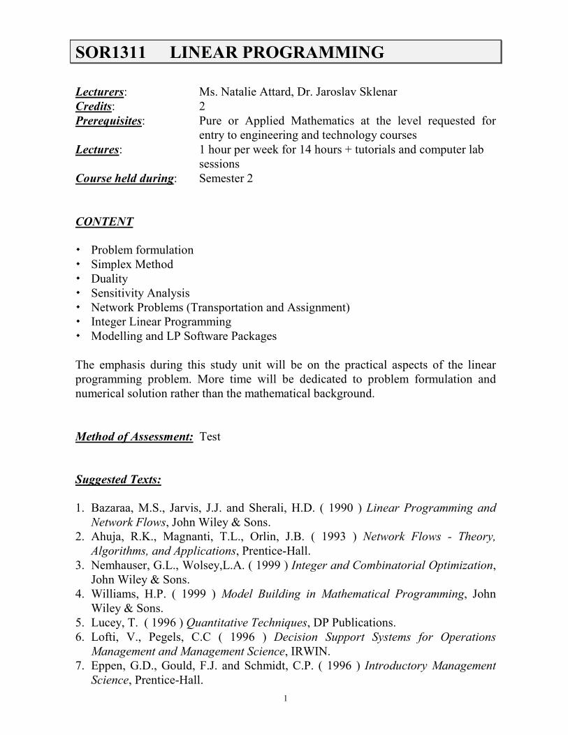
Consider the following system of inequalities

4

2

2

, 0

x y

x

y

x y

+ ≤

≤

≤

≥

Converting the problem into standard form yields:

x + y + s1 = 4

x + s2 = 2

y + s3 = 2

x, y, s1, s2, s3 ≥ 0

The projection of this 5-dimensional problem into the x-y plane is shown

in the following figure.

16

Clearly from the figure, there four corners, three of them nondegenerate - (0,0), (0,2),

(2,0) (corner point occurs at the intersection of two lines) and one degenerate (2,2)

(corner point occurs at the intersection of more than two lines – 3 in this case). The

following table shows the correspondence between the basic feasible solutions to the

LP and the extreme points of the feasible region.

Corner (x,y) Basic variables Nonbasic variables Corresponds to

Corner Point

(0,0) s1 = 4, s2 = 2, s3 = 2 x, y A

(2,0) x = 2, s1 = 2, s3 = 2 s2, y B

(2,2)

x = 2, y = 2, s3 = 0

x = 2, y = 2, s2 = 0

x = 2, y = 2, s1 = 0

s1, s2

s1, s3

s2, s3

C

(0,2) y = 2, s1 = 2, s2 = 2 x, s3 D

Note that the degenerate corner has three zero variables (s1, s2, s3), so it is possible to

select three different pairs of nonbasic variables. Recall that the above picture is in

fact a projection into the x-y plane, because after converting inequalities into

equalities the feasible region is a 5-dimensional object (called polyhedron).

The geometrical concept says, that an optimal solution exists always at a corner

(there can be more optimal solutions, for example a line connecting two corners).

This is another way how to express the basic idea of the simplex method: moving

along the edges of the n-dimensional polyhedron until an optimal corner is found.

17

Chapter 4: The Simplex Method

Simplex Algorithm informally:

Find an initial basic feasible solution

While (there is a possible improvement)

Find the most promising improvement direction

Move as much as possible in this direction to the next corner

Adjust the model accordingly

EndWhile

So there are several problems involved in the simplex method. The next paragraphs

explain the basic ideas, for details see examples. Practical implementation of the

method is based on the so-called Simplex Table that contains all LP model

parameters arranged in a way that supports the operations. Note also, that there are

several modifications, how to arrange and use the simplex table.

1. The way how to find an initial basic feasible solution (IBFS) depends on the type

of constraints. Typical example for maximization problems with all constraints ≤, the so-called all slack model, are zero solution variables (the ones that are used in

the original inequality model) and positive slacks representing the unused

resources. Note that there is exactly one basic variable for each constraint. For

problems with ≥ constraints and/or equalities we need the so-called artificial

variables – see later.

2. The most promising improvement can be found from the coefficients of the

objective function (OF). Let’s assume that in a certain maximization model the

initial point has all the activities nonbasic (equal to zero). Improving in the first

step means inserting a certain activity as a basic one. That will force one of the

current basic variables (slacks) out of the basic set - see the next paragraph. The

most promising variable has the maximum positive coefficient in the OF (because

the OF is linear, these coefficients are partial derivatives of the objective function

with respect to particular variables). The column that contains the maximum

coefficient is called pivot column. If there is no positive coefficient, the optimum

(maximum) has been found. Note that this is true for the first iteration. In fact the

simplex table is (typically) created in such a way that its objective row (z - row)

always contains the so-called negative reduced costs (negative partial derivatives

of the objective with respect to particular nonbasic variables) and zeros in basic

columns.

3. Selecting a nonbasic variable to be inserted as a basic one defines the direction of

the move in the n-dimensional space. The maximum distance of the move is given

18

by the natural requirement to keep feasibility - it is not possible to go out of the

feasible region. A certain constraint will thus stop the movement, so the

corresponding slack will become zero that means it will change from a basic into a

nonbasic variable. The constraint involved can be found by using the coefficients

of the constraint matrix, namely in the pivot column, and the right hand side

(RHS) values. The ratio of the RHS value and the pivot column coefficient defines

the maximum possible increase of the nonbasic variable allowed by this particular

constraint. Obviously the minimum value is chosen. The row that contains the

minimum value (the pivot row) thus defines the distance of the move (the ratio)

and the basic variable that becomes nonbasic. The intersection of the pivot row

and the pivot column is called pivot element.

4. To introduce a nonbasic variable it is necessary to take the amounts of all

resources needed by this variable. This is performed by making zeros in the pivot

column, except the pivot element, that is 1. The zero in the last row represents the

fact, that the variable is basic. The values in the OF row have been changed, but

they always represent the change of the objective caused by introducing one unit

of the nonbasic variable into the solution.

Formal justification of the ideas outlined above is given in Appendix A. The

following paragraph gives the algorithm of the simplex method that covers most

practical cases.

The Simplex Algorithm:

1. Create the initial (possibly inconsistent) simplex table:

BV xN xB RHS

xB

N

I

b

z - cN - cB 0

Where (N I) = A is the matrix of coefficients with unity matrix in last m

columns.

b = vector of right-hand sides

cN = objective coefficients of nonbasic variables

cB = objective coefficients of basic variables

xB = basic variables

xN = nonbasic variables

2. Make the table consistent by performing such row operations, that the values in

the z-row in basic columns are zero. This is not necessary for all slack models.

19

3. Use Optimality test to check whether the table is optimal:

Minimization: All negative reduced costs (z-row entries) must be negative or

zero.

Maximization: All negative reduced costs (z-row entries) must be positive or

zero.

If the table is optimal go to the step 6. If not, select the entering variable:

Minimization: Select variable with the greatest positive value.

Maximization: Select variable with the most negative value.

Entering variable defines the pivot column.

4. Use Feasibility test to find the leaving variable:

Compute the ratios of right-hand sides and positive coefficients in the

pivot column. Ignore rows with non-positive coefficients. If there are no

positive coefficients, the problem is unbounded. Select the row with the

minimum ratio to find the pivot row and the leaving variable.

5. Pivot on pivot element: perform such row operations to create zeros in the pivot

column except the pivot element that has to be 1. Go to the step 3.

6. Interpret the optimal simplex table that contains (among others):

- The objective value

- Values of basic variables (nonbasic ones are zero)

- Shadow costs of resources in slack columns

- Penalties caused by introducing nonbasic variables

Note: To find fast an initial basic feasible solution for ≥ inequalities, subtract a surplus variable and

add an artificial variable.

Ex: 4x1 + 5x2 ≥ 150 → 4x1 + 5x2 - y1 = 130 → 4x1 + 5x2 - y1 + a1 = 130 , y1, a1 ≥ 0 a1 = mathematical tool without practical (model) interpretation

Initial basic feasible solution: x1 = 0, x2 = 0, y1 = 0, a1 = 130

To find fast an initial basic feasible solution for an equality constraint, add an artificial variable.

Ex: 4x1 + 5x2 = 130 → 4x1 + 5x2 + a1 = 130 , a1 ≥ 0

a1 = mathematical tool without practical (model) interpretation

Initial basic feasible solution: x1 = 0, x2 = 0, a1 = 130

20

Though it is used only rarely in linear programming, we can convert an equality into two

inequalities.

Ex: 4x1 + 5x2 = 150 → 4x1 + 5x2 ≤ 150

4x1 + 5x2 ≥ 150

If one of these two inequalities is multiplied by -1, we get two inequalities with the same signs.

Now we can summarize. To use the simplex method, all inequalities are first converted to equalities

and also there must be trivial initial basic feasible solution. To do it we follow these rules:

1. Add a slack variable in each ≤ inequality constraint.

2. Subtract a surplus variable in each ≥ inequality constraint and add an artificial variable.

3. Add an artificial variable in each equality constraint.

Ex: The constraints x1 ≤ 4

x2 ≥ 3

x1 + x2 = 10

x1 , x2 ≥ 0

Can be converted into these equalities:

x1 + s1 = 4

x2 - y2 + a1 = 3

x1 + x2 + a2 = 10

x1 , x2 , s1 , y2 , a1 , a2 ≥ 0

With the following trivial initial basic feasible solution:

x1 = x2 = y2 = 0, s1 = 4, a1 = 3, a2 = 10

In the objective function the coefficients of slack and surplus variables are zero, because the only

use of these variables is to balance inequalities. They do not affect the objective value.

During the solution process it is necessary to force the artificial variables out of the optimum

solution (they are just used as a tool to start the optimization process). There are two methods to do

so:

M-method penalizes artificial variables by such coefficients in the objective function that the

optimization process will eliminate them automatically. Namely use a certain very big value M for

minimization and -M for maximization respectively.

Two Phase method first minimizes the sum of artificial variables. When zero is reached, the

second phase continues from the solution reached by the first phase (without artificial variables) to

optimize the original objective.

21

Example: Find the optimum production plan for the following problem:

Product Quantity Machine

Hours Components Alloy Limits Contribution

A x1 2 1 2 - 8

B x2 3 - - ≤50 5

C x3 1 1 4 - 10

Amount Available 400 150 200

1. Express the problem in standardized format

1 2 3

1 2 3

1 3

1 3

2

1 2 3

max 8 5 10

subject to

2 3 400

150

2 4 200

50

, , 0

x x x

x x x

x x

x x

x

x x x

+ +

+ + ≤

+ ≤

+ ≤

≤

≥

2. Convert inequalities into equalities by adding the slack variables

1 2 3 4

1 3 5

1 3 6

max

subject to

2 3 400

+ 150

2 4 +

z

x x x x

x x x

x x x

+ + + =

+ =

+ =

2 7

1 2 3 4 5 6 7

1 2 3 4 5 6 7

200

50

8 5 10 0 0 0 0 0

, , , , , , 0

x x

z x x x x x x x

x x x x x x x

+ =

− − − − − − − =

≥

Interpretation of Slack variables:

x4 - unused machine hours

x5 - unused components

x6 - unused alloy

x7 - amount of product B not produced

22

3. Set up the initial simplex table:

Products Slack Variables Solution

Variable x1 x2 x3 x4 x5 x6 x7

Solution

Quantity

x4 2 3 1 1 0 0 0 400

x5 1 0 1 0 1 0 0 150

x6 2 0 4 0 0 1 0 200

x7 0 1 0 0 0 0 1 50

z -8 -5 -10 0 0 0 0 0

IBFS: 4 5 6 7 1 2 3

BV

= ( , , , , , , ) = (400,150, 200,50,0,0,0)

NBV

x x x x x x x����� �����

Tx

Initial Objective function value: 0z =

4. Optimality Test: Is the current BFS optimal? – No (since values in z row are not

all positive – maximization)

i. Select the highest negative contribution in the z row (i.e. –10

corresponding to x3) ⇒ x3 is the entering variable (x3 becomes a BV,

pivot column = column 3)

ii. Ratio Test: Which current BV has to be reduced to zero (i.e. become a

NBV)?

3

400

1

150

1min 50

200

4

50

0

x

⇒ = =

23

The product of x3 can be increased by 50 (pivot row = row 3), hence x6 must be

reduced to 0, and thus becomes a NBV.

Interpretation: instead of x6 the basic variable will be x3 (no unused alloy, all alloy

used to produce 50 units of product C).

Consequence: production of 50 units of product C will also affect other resources.

Thus, we need to find the new values of the other BV.

5. Ring the element in both the pivot row and pivot column (pivot element = 4).

Divide all the elements in the identified row (x6) by the pivot element (4) and

change the solution variable (i.e. x6 x3)

New Row 3 is:

x3 0.5 0 1 0 0 0.25 0 50

New Simplex Table is:

Products Slack Variables Solution

Variable x1 x2 x3 x4 x5 x6 x7

Solution

Quantity

x4 2 3 1 1 0 0 0 400

x5 1 0 1 0 1 0 0 150

x3 0.5 0 1 0 0 0.25 0 50

x7 0 1 0 0 0 0 1 50

z -8 -5 -10 0 0 0 0 0

6. Make all other elements in the pivot column equal to zero by repetitive row by

row operations:

i. New Row 1 = Old Row 1 – Row 3

x4 2 3 1 1 0 0 0 400

- x3 0.5 0 1 0 0 0.25 0 50

New

Row 1

1.5 3 0 1 0 -0.25 0 350

ii. New Row 2 = old row 2 – Row 3

iii. Row 4 = already zero

iv. Row 5 = old row 5 + 10(Row 3)

24

New table is:

Products Slack Variables Solution

Variable x1 x2 x3 x4 x5 x6 x7

Solution

Quantity

x4 1.5 3 0 1 0 -0.25 0 350

x5 0.5 0 0 0 1 -0.25 0 100

x3 0.5 0 1 0 0 0.25 0 50

x7 0 1 0 0 0 0 1 50

z -3 -5 0 0 0 2.5 0 500

New BFS is:

3 4 5 7 1 2 6

BV

= ( , , , , , , ) = (50,350,100,50,0,0,0)

NBV

x x x x x x x����� �����

Tx

New objective function value z = 500.

7. Repeat steps 4, 5 and 6 until there are no negative values in the z row. (i.e. no

improvement is possible).

Simplex Table after next step:

Products Slack Variables Solution

Variable x1 x2 x3 x4 x5 x6 x7

Solution

Quantity

x4 1.5 0 0 1 0 -0.25 -3 200

x5 0.5 0 0 0 1 -0.25 0 100

x3 0.5 0 1 0 0 0.25 0 50

x2 0 1 0 0 0 0 1 50

z -3 0 0 0 0 2.5 5 750

New BFS is:

2 3 4 5 1 6 7

BV

= ( , , , , , , ) = (50,50,200,100,0,0,0)

NBV

x x x x x x x����� �����

Tx

New Objective function value z = 750.

Interpretation: Produce maximum possible quantities of product B (since x1 and x6

are zero) and product C (since x7 is zero).

25

Optimal Simplex Table

Products Slack Variables Solution

Variable x1 x2 x3 x4 x5 x6 x7

Solution

Quantity

x4 0 0 -3 1 0 -1 -3 50

x5 0 0 -1 0 1 -0.5 0 50

x1 1 0 2 0 0 0.5 0 100

x2 0 1 0 0 0 0 1 50

z 0 0 6 0 0 4 5 1050

Interpretation of the optimal simplex table:

Contribution z = 1050

Production: 100 units of product A (x1)

50 units of product B (x2)

no units of product C (x3)

Unused (abundant) resources: 50 machine hours (x4)

50 components (x5)

Scarce resources: Alloy (x6 = 0). All alloy is used.

Limitation on product B is exhausted (x7 = 0)

Shadow prices:

i. 4 (contributing to alloy (x6))

ii. 5 (contributing to B limitation (x7))

iii. 6 (contributing to x3)

Interpretation of shadow prices:

i. If RHS of alloy constraint is increased/decreased by 1 the total contribution

would increase/decrease by 4.

ii. If RHS of B limitation constraint is increased/decreased by 1 the total

contribution, will increase/decrease by 5.

iii. If production of product C (x3) is increased by 1 the contribution will be 6

units less.

26

Chapter 5: Duality

Every LP model (primal) has its dual model, that can be created by conversion rules

that in case of canonical models (all inequalities of the same type) are like that:

Min cTx Max bTw

ST Ax ≥ b ST ATw ≤ c

x ≥ 0 w ≥ 0

Note that:

1. Maximization becomes minimization and vice versa.

2. RHS values of the primal are OF coefficients of the dual.

3. Primal OF coefficients are RHS values of the dual.

4. Transpose of the primal constraint coefficients matrix makes the dual

constraint matrix. It is also possible to express this by changing order of

multiplication in the dual model.

5. Change the inequality signs of constraints ( ≥ → ≤ , ≤ → ≥ ).

Applying the same rules to the dual model creates the primal one (so the names just

show which was the original one from the application point of view).

Example:

Primal : Min 3x1 + 4x2 Dual : Max 3w1 + 10w

ST 3x1 + 4x2 ≥ 3 ST 3w1 + 6w2 ≤ 3

6x1 + 9x2 ≥ 10 4w1 + 9w2 ≤ 4

x1,2 ≥ 0 w1,2 ≥ 0

The so-called basic theorem of duality limits the number of possible combinations

of primal and dual models. Actually only four out of nine combinations are possible:

Theorem: For any pair of dual models only these possibilities can occur:

1. Both have optimal solution with the same objective value.

2. Both are infeasible.

3. One is unbounded, the other is infeasible.

27

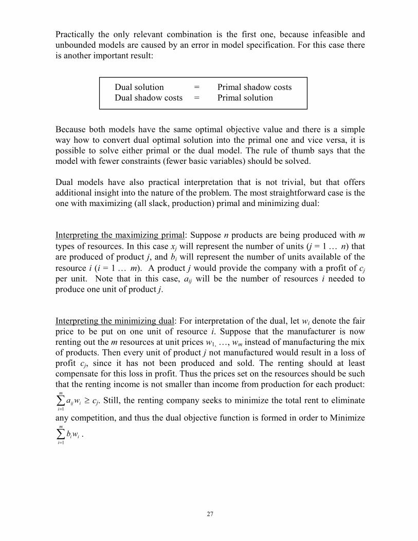
Practically the only relevant combination is the first one, because infeasible and

unbounded models are caused by an error in model specification. For this case there

is another important result:

Dual solution = Primal shadow costs

Dual shadow costs = Primal solution

Because both models have the same optimal objective value and there is a simple

way how to convert dual optimal solution into the primal one and vice versa, it is

possible to solve either primal or the dual model. The rule of thumb says that the

model with fewer constraints (fewer basic variables) should be solved.

Dual models have also practical interpretation that is not trivial, but that offers

additional insight into the nature of the problem. The most straightforward case is the

one with maximizing (all slack, production) primal and minimizing dual:

Interpreting the maximizing primal: Suppose n products are being produced with m

types of resources. In this case xj will represent the number of units (j = 1 … n) that

are produced of product j, and bi will represent the number of units available of the

resource i (i = 1 … m). A product j would provide the company with a profit of cj

per unit. Note that in this case, aij will be the number of resources i needed to

produce one unit of product j.

Interpreting the minimizing dual: For interpretation of the dual, let wi denote the fair

price to be put on one unit of resource i. Suppose that the manufacturer is now

renting out the m resources at unit prices w1, …, wm instead of manufacturing the mix

of products. Then every unit of product j not manufactured would result in a loss of

profit cj, since it has not been produced and sold. The renting should at least

compensate for this loss in profit. Thus the prices set on the resources should be such

that the renting income is not smaller than income from production for each product:

∑=

m

i

iijwa1

≥ cj. Still, the renting company seeks to minimize the total rent to eliminate

any competition, and thus the dual objective function is formed in order to Minimize

∑=

m

i

iiwb1

.

28

Example: Maximizing Primal – Minimizing Dual Interpretation: A company

produces two types of paints: paint A and paint B. Production of both paints is made

by the use of two raw materials M1 and M2. The production involves mixing

specific quantities of each material for every ton of either paint A or B. These

quantities in tons are summarized in the following table:

Paint A (x1) Paint B (x2) Available Resources

M1 6 4 24

M2 1 2 6

Profit/ton of paint in

Lm 1000

5 4

In addition, the maximum production of paint B should not exceed 2 tons, and the

production of paint B should not exceed the production of paint A by more than 1

ton. The company wants to maximize profit.

The primal model:

1 2

1 2

1 2

1 2

2

1 2

max 5 4

. .

6 4 24

2 6

1

2

, 0

z x x

s t

x x

x x

x x

x

x x

= +

+ ≤

+ ≤

− + ≤

≤

≥

The dual model:

1 2 3 4

1 2 3

1 2 3 4

1 2 3 4

min 24 6 2

. .

6 5

4 2 4

, , , 0

v w w w w

s t

w w w

w w w w

w w w w

= + + +

+ − ≥

+ + + ≥

≥

`

Suppose now that the company instead of manufacturing the paints wants to sell the

resources. Then w1,w2,w3 and w4 will denote the unit prices that are decided by the

company for the selling. Now, if one unit of paint A say (x1) is not manufactured

then this would results in a loss of Lm5,000 per ton of profit (since z = 5x1 + 4x2).

Thus, not to run at a loss, the cost of selling should not result in a diminishing profit

compared with manufacturing i.e. 1 2 36 5w w w+ − ≥ (×Lm1000), because the

29

coefficients 6, 1 and –1 represent the amount of resources needed to produce one

unit of paint A (one unit of x1). Similarly for paint B.

Since the company’s target is to eliminate competition, it should aim to minimize the

price of selling the resources i.e. min 1 2 3 424 6 2z w w w w= + + +` but at the same time

without producing any loss in profit. This justifies the dual LP model.

Note that the last two resources are not the material ones. The third resource can be

described as “possibility to produce more paint B than paint A”. Each additional ton

of the paint A in fact decreases the “use” of this resource. That’s why the value -1 in

the matrix. Each additional ton of the paint B makes use of one unit of this resource, that’s why the value +1 in the matrix. The fourth resource can be described as

“possibility to produce paint B”. By each ton of B we are utilizing one unit of that

resource, that’s why the matrix value is 1. RHS values are availability of these

resources: 1 as the maximum difference B-A, 2 as the maximum production of B.

Example: Minimizing Primal – Maximizing Dual Interpretation:

Suppose that a family is trying to make a minimal cost diet from six available primary foods (called 1,2,3,4,5,6) so that the diet contains at least 9 units of vitamin

A and 19 units of vitamin C. The following table shows the data on the foods.

Number of Units of

Nutrients per kg of Food

Minimum Daily Requirement of

Nutrient

Nutrient 1 2 3 4 5 6

Vitamin A 1 0 2 2 1 2 9

Vitamin C 0 1 3 1 3 2 19

Cost of food (c/kg) 35 30 60 50 27 22

The primal model:

1 2 3 4 5 6

1 3 4 5 6

2 3 4 5 6

1 6

min 35 30 60 50 27 22

. .

+2 +2 + +2 9

+3 + +3 +2 19

,... 0

z x x x x x x

s t

x x x x x

x x x x x

x x

= + + + + +

≥

≥

≥

30

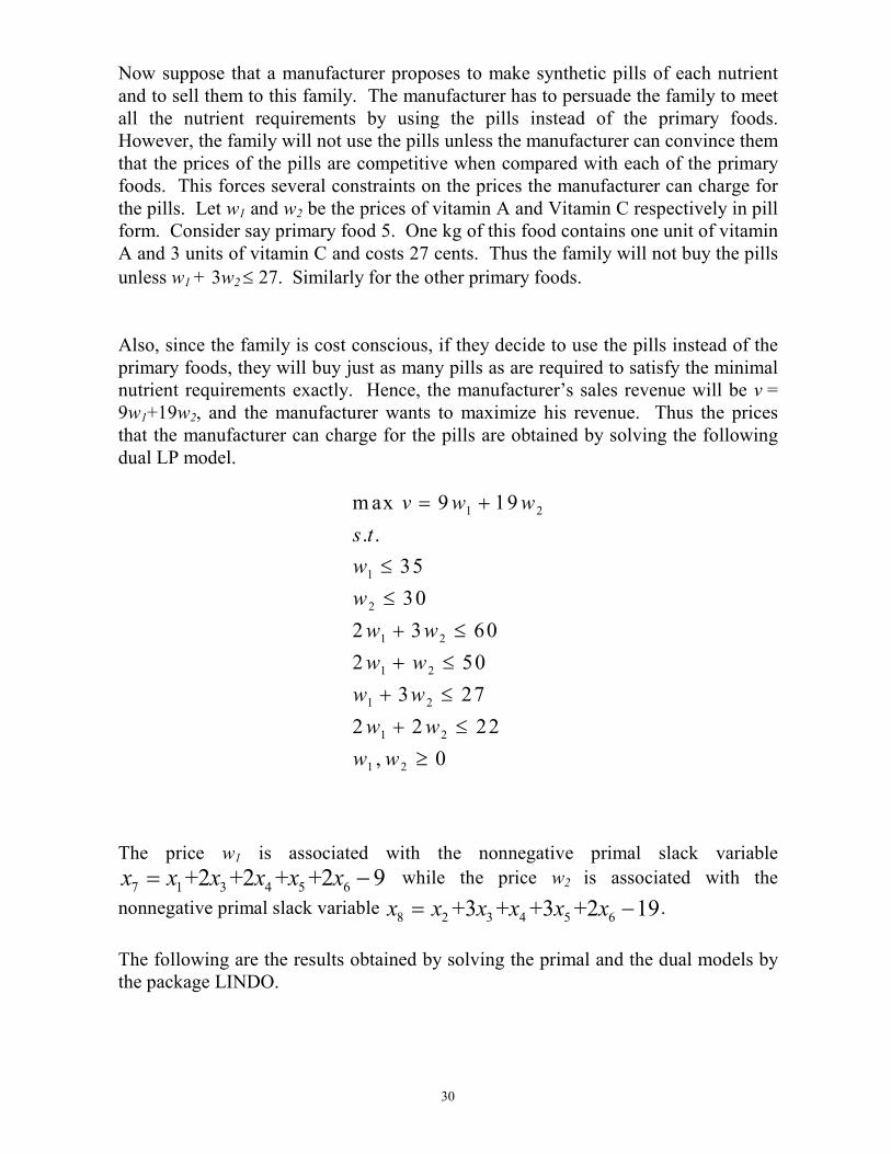
Now suppose that a manufacturer proposes to make synthetic pills of each nutrient

and to sell them to this family. The manufacturer has to persuade the family to meet

all the nutrient requirements by using the pills instead of the primary foods. However, the family will not use the pills unless the manufacturer can convince them

that the prices of the pills are competitive when compared with each of the primary

foods. This forces several constraints on the prices the manufacturer can charge for

the pills. Let w1 and w2 be the prices of vitamin A and Vitamin C respectively in pill form. Consider say primary food 5. One kg of this food contains one unit of vitamin

A and 3 units of vitamin C and costs 27 cents. Thus the family will not buy the pills

unless w1 + 3w2 ≤ 27. Similarly for the other primary foods.

Also, since the family is cost conscious, if they decide to use the pills instead of the

primary foods, they will buy just as many pills as are required to satisfy the minimal nutrient requirements exactly. Hence, the manufacturer’s sales revenue will be v =

9w1+19w2, and the manufacturer wants to maximize his revenue. Thus the prices

that the manufacturer can charge for the pills are obtained by solving the following

dual LP model.

1 2

1

2

1 2

1 2

1 2

1 2

1 2

max 9 19

. .

35

30

2 3 60

2 50

3 27

2 2 22

, 0

v w w

s t

w

w

w w

w w

w w

w w

w w

= +

≤

≤

+ ≤

+ ≤

+ ≤

+ ≤

≥

The price w1 is associated with the nonnegative primal slack variable

7 1 3 4 5 6+2 +2 + +2 9x x x x x x= − while the price w2 is associated with the

nonnegative primal slack variable 8 2 3 4 5 6+3 + +3 +2 19x x x x x x= − .

The following are the results obtained by solving the primal and the dual models by the package LINDO.

31

Results:

PRIMAL:

OBJECTIVE FUNCTION VALUE

1) 179.0000

VARIABLE VALUE REDUCED COST

X1 0.000000 32.000000 X2 0.000000 22.000000

X3 0.000000 30.000000

X4 0.000000 36.000000

X5 5.000000 0.000000

X6 2.000000 0.000000

SLACK OR SURPLUS SHADOW COSTS/PRICES

X7 0.000000 -3.000000 X8 0.000000 -8.000000

DUAL:

OBJECTIVE FUNCTION VALUE

1) 179.0000

VARIABLE VALUE REDUCED COST W1 3.000000 0.000000

W2 8.000000 0.000000

SLACK OR SURPLUS SHADOW COSTS/PRICES W3 32.000000 0.000000

W4 22.000000 0.000000

W5 30.000000 0.000000

W6 36.000000 0.000000 W7 0.000000 5.000000

W8 0.000000 2.000000

32

Recall that in an LP model, the rate of change in the optimal objective function value

per unit change in the Right Hand Side values of each constraint (keeping other

values fixed) is known as the shadow costs.

Thus in this case, the shadow costs of the primal LP problem represents the amount

of extra money the family has to spend by using an optimum diet, per unit increase in

the requirement of that vitamin i.e. 3 cents for vitamin A and 8 cents for vitamin C. Thus, the price charged by the manufacturer, per unit of vitamin, is acceptable to the

family if the price of each vitamin is less than or equal to the shadow cost of that

vitamin in the primal problem. Therefore, in order to maximize his revenue, the

manufacturer must price the vitamins 3 and 8 cents per unit respectively.

Hence, in an optimum solution of the dual problem, the prices w1 and w2 correspond

to the shadow costs of vitamins A and C respectively. Similarly, in any LP, the dual

variables are the shadow costs/prices of the resources associated with the constraints

in the primal problem.

33

Chapter 6: Network Problems

There is a group of linear programming problems defined on networks (directed

graphs) that have many special properties. These properties enable some fast special

algorithms and also an efficient version of simplex method called network simplex

method. This chapter introduces the basic ideas, some special practically important versions of network problems (transportation, assignment) and presents selected

algorithms. Knowledge of graph theory is not a precondition; all used terms are

defined here. Examples and drawings will be added during lectures.

General minimum cost network flow problem

Definition: Network is a simple directed graph (digraph) N = (V, A) made of a finite

non-empty set V = {v1, v2, ... vm} of vertices (nodes) and a set A ⊆ V × V of directed

arcs where each arc is an ordered pair of vertices (i, j) ,i,j = 1 … m. Note that

between two vertices in one direction there can be mostly one arc – simple graph.

Example: Let V = {1,2,3,4,5,}, A = {(1,2),(1,3),(2,3),(2,4),(2,5),(3,4),(3,5),(4,5)}.

The network representing the above data is shown below.

In this text we shall assume that loops do not exist: (i, i) ∉ A, i = 1 … m. Also let n

be the number of arcs. Note that in graph theory n usually means the number of

vertices. Here we shall have one variable for each arc, so to keep compatibility with linear programming notation (n = number of variables) the meaning of symbols is

reversed.

A common scenario of a minimum cost network flow problem arising in industrial

logistics concerns the distribution of a product from plants (origins) to consumer markets (destinations). The total number of units produced at each plant and the total

number of units required at each market are assumed to be known. The product need

not be sent directly from source to destination, but may be routed through

intermediary points reflecting warehouses or distribution centers. Further, there may

be capacity restrictions that limit some of the shipping links. The objective is to minimize the cost of producing and shipping the products to meet the consumer

demand.

Thus, the minimum cost network flow problem is based on these assumptions: Let

flow (movement of any commodity through an arc – for example tons of oil per hour in an oil pipeline network, cubic meters of water per minute in a city water system,

1 3 5

2 4

34

pulses per second in a communications network, or the number of vehicles per hour

on a regional highway system) in the arc (i, j) connecting vertices i and j (in this

direction) be represented by xij. Then, for each arc, there is generally:

- A lower bound on the flow lij ≤ xij (mostly 0 – nonnegativity)

- An upper bound on the flow uij ≥ xij (interpreted as the arc’s capacity)

- A certain cost cij paid for unit flow through the arc (i, j). The total cost that we pay for the flow through the arc (i, j) is then cijxij.

Flow is in a certain way inserted into the network and somehow removed. This can

be generalized by introducing for each vertex i:

- An external input flow bi+

- An external output flow bi-.

Let Pi be the set of predecessors of the vertex i (the set of vertices where arcs ending in i start) and similarly let Si be the set of successors of i. Graphically:

Pi i Si

bi

+ bi-

The general condition that is supposed to be satisfied with all network problems is

flow conservation stating that flow must neither originate, nor vanish in a vertex. In other words, for each vertex the total flow out must be equal to the total flow in:

, 1...i i

ij i ki i

j S k P

x b x b i m− +

∈ ∈

+ = + =∑ ∑

Simple rearrangement gives:

, 1...i i

ij ki i i i

j S k P

x x b b b i m+ −

∈ ∈

− = − = =∑ ∑

According to the value of bi there are three types of vertices:

- Source with bi > 0 that adds flow to the network,

- Sink with bi < 0 that removes flow from the network,

- Transshipment vertex with bi = 0.

35

Practically, source nodes may represent plants for example, which supply bi units of

desalinated water say. Sink node may then represent a number of cities, which

require bi units as will be indicated by the negative signs. The remaining nodes have no net supply or demand bi = 0; they are intermediate points, referred to as

transshipment nodes, for example special pumping stations used to transmit water

from origin to destination.

From the linear programming point of view the above equations represent

restrictions. The objective is to find the minimum-cost flow pattern to fulfil

demands. All these can now be expressed in matrix form in usual way:

Min z = cTx

ST Ax = b

L ≤ x ≤ U

Where c, L and U are n - vectors of unit costs, lower bounds and upper bounds

respectively. The matrix A has m rows (each row represents one vertex) and n

columns (one column for each arc). Compared with other LP problems, there are few

differences. First there are double subscripts of the vectors x, c, L, U and columns of

A. This is just a formal difference in notation to avoid separate indexing of vertices

and arcs. Lower and upper bounds represent generally additional 2n constraints.

Lower bounds are mostly zero – usual nonnegativity requirement. If not, a simple

change of variables can be used to replace l ≤ x by 0 ≤ x-l = x*. Also upper bounds

can be eliminated if necessary by replacing a bounded variable by two variables: x ≤ u can be replaced by x1 – x2 ≤ u, where x1 and x2 are nonnegative and unbounded. Of course in the model x is replaced by x1 – x2 and we need to add additional

constraints. So without loss of generality (and with some modifications in the model)

the bounds can be ignored.

1 4

3

2 5

[40]

[50]

[-50]

[-60]

Source

Plant 1

Source

Plant 2

Transshipment

Node – pumping

station

Sink

City 1

Sink

City 2

Supplly Demand

Lm 5

Lm 3

Lm 2

Lm 7

Lm 1

Lm 8 Lm 4

Unit Cost

(20,35)

(4,10)

(0,∞ )

(10,30)

(30,60) (0,∞ )

(0,∞ )

Lower bound Upper bound (Capacity)

36

Example: Consider the following network:

The above network yields the following LP problem:

x12 x13 x14 x23 x25 x34 x35 x46 x56 bi

Min 3 4 1 5 6 1 2 2 4

Node 1 1 1 1 100

Node 2 -1 1 1 200

Node 3 -1 -1 1 1 50

Node 4 -1 -1 1 -150

Node 5 -1 -1 1 -80 Node 6 -1 -1 -120

lij 0 0 50 0 0 70 0 100 0

uij ∞ ∞ ∞ ∞ ∞ ∞ ∞ ∞ ∞

(3 4 1 5 6 1 2 2 4)

1 1 1 0 0 0 0 0 0

1 0 0 1 1 0 0 0 0

0 -1 0 -1 0 1 1 0 0

0 0 -1 0 0 -1 0 1 0

0 0 0 0 -1 0 1 0 1

0 0 0 0 0 0 0 1 1

100

200

50

150

80

120

T =

− = − − −

− − −

c

A

b =

Consider for example the flow x14, which must satisfy 1450 x≤

The lower bound 50 is changed to 0 as follows:

1 4

6

2 5

3

Lm 5 Lm 3

Lm 4

Lm 6

Lm 1

Lm 2 Lm 4

Lm 2 Lm 1

[100] [-150]

[-120]

[50]

[200] [-80]

(50,∞ )

(0,∞ ) (70,∞ ) (100,∞ )

(0,∞ ) (0,∞ ) (0,∞ )

(0,∞ )

(0,∞ )

37

14

14

* *

14 14 14

50

50 0

0 where = 50

x

x

x x x

≥

− ≥

⇒ ≥ −

This results in the following table:

x12 x13 *

14x x23 x25 x34 x35 x46 x56 bi

Min 3 4 1 5 6 1 2 2 4

Node 1 1 1 1 50

Node 2 -1 1 1 200

Node 3 -1 -1 1 1 50

Node 4 -1 -1 1 -100 Node 5 -1 -1 1 -80

Node 6 -1 -1 -120

lij 0 0 0 0 0 70 0 100 0

uij ∞ ∞ ∞ ∞ ∞ ∞ ∞ ∞ ∞

Repeating the same procedure for x34 and x46, the following LP problem is obtained:

x12 x13 *

14x x23 x25 *

34x x35 *

46x x56 bi

Min 3 4 1 5 6 1 2 2 4

Node 1 1 1 1 50

Node 2 -1 1 1 200 Node 3 -1 -1 1 1 -20

Node 4 -1 -1 1 -130

Node 5 -1 -1 1 -80

Node 6 -1 -1 -20

lij 0 0 0 0 0 0 0 0 0

uij ∞ ∞ ∞ ∞ ∞ ∞ ∞ ∞ ∞

What makes the networks problems special are the properties of A and b (in

balanced case). Note that the feasibility condition suggests that for A there is in each

row (vertex):

- +1 for starting arcs

- -1 for ending arc

- Zeros otherwise.

Similarly in each column (arc) there is:

100 - 50

-150 + 50

38

- +1 for the starting vertex

- -1 for the ending vertex

- Zeros otherwise.

Especially columns are very special: once +1, once –1, m-2 zeros. The sum of rows

is thus 0, so the rows are linearly dependent. It means that the maximum rank of A is

m-1 (in fact it is exactly m-1). Here we assume that n ≥ m that is satisfied for all

connected networks that are not trees – see later. For a balanced network (supply =

demand) where the total inserted flow is equal to the total flow removed we have:

1

0m

i

i

b=

=∑

Unbalanced networks can be balanced by adding artificial vertices and arcs that

make the difference. Let S be the total supply to the network and D the total demand:

: 0 : 0i i

i i

i b i b

S b D b> <

= = −∑ ∑

A balanced network has S = D. This is the balancing algorithm:

- If S > D (excess supply) then add an artificial vertex with demand S-D, and

add artificial arcs connecting all sources to this artificial vertex. These new

arcs have costs that correspond to the cost (if any) of excess production.

- If D > S (excess demand) then add an artificial vertex with supply D-S, and

add artificial arcs connecting this artificial vertex to all sinks. These new arcs

have costs that correspond to the cost (if any) of unmet demand.

Without loss of generality we shall assume that a network is balanced. Obviously flow through artificial arcs represents excess supply or unmet demand respectively.

During optimization there is no difference between real and artificial arcs and

vertices.

Special cases of network flow problems

The general minimum cost network flow problem defined above is also called

Transshipment problem, because there can be all three types of vertices.

Transportation problem has only sources and sinks and every arc goes from a

source to a sink. Conservation constraints have one of two forms:

ij i

j

x b=∑ for a source with bi > 0, and

39

ki i

k

x b− =∑ for a sink with bi < 0.

Transportation problems model direct movement of goods from suppliers to

customers with cij coefficients interpreted as the unit cost of transportation from a

particular supplier to a particular customer. The objective is to determine the amounts to be shipped from the origins (sources) to the sinks (destinations) at

minimum cost, while satisfying the supply and demand limitations.

Assignment problem is a special case of the transportation problem, where bi = 1

for a source and bi = -1 for a sink. For a balanced problem there are the same number

m/2 of sources and sinks. Assignment typically models assigning people to jobs with

cij coefficients interpreted as the value of a person if assigned to a particular job (a

job that matches a worker’s skill costs less than a job in which the operator is not as skillful). Objective value is then interpreted as total profit (maximization) or total

cost (minimization) of all assignments. Later we shall see that the integrity of flows

is guaranteed, so the only possible values are 1 and 0. There is a special fast

algorithm for assignment.

Shortest path problem determines the shortest (fastest) path between an origin and

a destination. There are efficient shortest path algorithms in graph theory, but linear

programming can also solve the problem. Shortest path problem can be represented as a minimum cost network flow problem with one source (the origin) with supply

equal to 1, and one sink (the destination) with demand equal to 1. There are typically

many transshipment vertices. The cij coefficients are interpreted as lengths of arcs

(that can be generalized as time required to traverse an arc, or cost of using an arc).

Unlike in graph theory algorithms, the coefficients need not be nonnegative.

Maximum flow problem determines the maximum amount of flow that can be

moved through a network from the source to the sink. Because the external flow is

not known a-priori, a slight modification of the general problem is necessary. Probably the simplest one adds an artificial arc with infinite capacity from sink to

source that returns the flow back to the source. Then all vertices are transshipment

and the model maximizes the flow through the artificial arc. Let s be the source and

let t be the sink. This is then the model: Max xts, ST Ax=0, 0≤x≤U where U are the

capacities of arcs. Note that costs are not used in this model.

Note: The maximum flow problem has an interesting dual problem (knowledge of duality is

assumed here) that deals with cuts. A cut is defined as a division of the vertices into two disjoint

sets V1 and V2, the first V1 containing the source s, the second V2 containing the sink t:

V1 ∪ V2 = V, V1 ∩ V2 = ∅, s ∈ V1, t ∈ V2.

The capacity of the cut is the sum of the capacities of the arcs that lead from V1 to V2.

40

Now let’s first rewrite the primal maximum flow problem:

Max z = xts

ST

0 , 1...

0 , ( inequalities)

i i

ij ki

j S k P

ij ij

x x i m

x u n

∈ ∈

− = =

≤ ≤

∑ ∑

The dual problem has one variable for each primal constraint, so there will be m+n dual variables.

Let’s call them yi , i = 1 … m for the first m flow conservation equalities and vij for the second

group of n capacity limitation inequalities. The dual objective coefficients are the RHS of primal

constraints, so the dual objective is

Min ij ijw u v=∑

Now let’s create dual constraints. There is one for each primal variable, it means one for each arc

(including the artificial one from t to s). Also note that the only non-zero primal objective

coefficient 1 corresponds to this arc. The capacity of this arc is infinite, so it is not included in the

second group of n capacity limitation inequalities. So we have these dual constraints:

yt – ys = 1 for the artificial arc

yi – yj + vij ≥ 0 for all the other arcs (i, j)

vij ≥ 0

The interpretation of the dual is the following: let yi=0 if vertex i is in the set V1, and let yi=1 if

vertex i is in the set V2. So the dual variables y define a cut. The first dual constraint guarantees

that s ∈ V1 and t ∈ V2. Let vij=1 if arc (i, j) connects V1 with V2 (the dual constraints guarantee this

fact) and let vij=0 otherwise. Then the dual objective is the capacity of the cut and the dual optimum

is the minimum capacity cut. Using the strong duality, we can formulate the famous max-flow min-

cut theorem: “maximum flow in a network is equal to the minimum of the capacities of all cuts in

the network”.

Maximum flow problem can be expanded to Minimum cost maximal flow

problem. To avoid possibly conflicting criteria, one way to solve this problem is the

following: first find the maximum flow without costs. Then minimize the total cost

provided the flow in the artificial arc is kept at maximum value (additional constraint). A modification of this problem is Minimum cost flow with given value

(or Minimum cost flow with given minimum acceptable value). Both can be solved by

the general minimum cost flow algorithm with one more constraint (= or ≥) on the

flow through the artificial arc.

There are other practically less significant special cases of the general minimum cost

network flow problem. Note that all network problems can be solved by the standard simplex method, so any LP solver can generally be used. There are two points to

mention. First network problems are mostly degenerate (many zero basic variables).

So there can be problems. On the other hand special properties of the matrix A of

network problems make it possible to use special algorithms faster than the standard simplex algorithm. Some will be presented even though with today’s fast computers

their use is justified only for very big models.

41

Transportation

Problem: minimization of total transportation costs of a certain commodity from n

sources to m destinations, based on known unit transportation costs from each

source to each destination and known amounts available (supplies) at each source and known demands of all destinations.

Note: The problem is balanced if the total supply is equal to the total demand.

Unbalanced problems can be balanced by adding a dummy row (dummy source)

or a dummy column (dummy destination) with zero costs and the supply or

demand that makes the balance. Interpretation: allocations to dummy cells

represent the fact, that the commodity is not transported (no satisfied demand for

a dummy row, or commodity left at source for a dummy column respectively). Next only balanced models are considered.

Example: Balance the next table.

Destinations A B C D

Sources Supply/Demand 20 30 15 5

I 40 2 4 1 6

II 20 4 3 3 3

III 20 1 2 5 2

LP model of a balanced transportation problem

1 j m

1 . cij = Unit cost of the i to j transportation

. si = Supply at i

i … cij xij dj = Demand at j

xij = Solution variable (amount transported from i to j) n

xij ≥ 0

∑∑= =

n

i

m

j

ijij xcMin1 1

∑=

==n

i

jij mjdx1

,2,1, �

∑=

==m

j

iij nisx1

,2,1, �

42

Notes: there are m×n solution variables and m+n equality constraints, but only m+n-

1 of them are independent, because the sum of rows is equal to the sum of

columns. So there are m+n-1 independent constraints that is also the number of

basic variables. Due to properties of the balanced matrix there are faster

methods to find an initial basic feasible solution and to perform simplex iterations.

Algorithm to find an initial basic feasible solution

While (there are less than m+n-1 allocations) do

Select a next cell (see the following algorithms)

Allocate as much as possible to this cell (this allocation is equal to the

minimum of the supply in the row and the demand in the column) Adjust the associated amounts of the supply and the demand (subtract the

allocation)

Cross out the column or the row with zero supply or demand, but not both !

EndWhile

Algorithms to select the next cell

1. North - West corner method

Start with the upper left cell

Allocate as much as possible

If row crossed move down, otherwise move right

Note: It may happen that a zero is allocated (a zero basic variable). After

allocating the bottom right entry, there will be exactly one uncrossed row

or column and m+n-1 allocations.

2. Least cost method

Next cell is the not allocated cell with minimum cost. Break ties arbitrarily.

Note: Not allocated cell is a cell whose row and column are not crossed. It may

happen that a zero is allocated (a zero basic variable). Stop if exactly one

row or column with zero supply or demand remains. This provides the

required m+n-1 allocations.

3. Vogel approximation method (VAM)

a) For each not crossed out row and column compute the penalty as the difference between the smallest and the next smallest costs in that row or

column. This has to be computed for each step (after crossing a row,

43

recalculate penalties in columns, after crossing a column, recalculate

penalties in rows).

b) Select a row or a column with the highest penalty. Break ties arbitrarily.

c) Allocate as much as possible to the cell with the minimum cost in the

selected row or column.

Note: If all uncrossed out rows and columns have zero remaining supply and

demand, determine the zero basic variables by the Least cost method. Stop

if exactly one row or column with zero supply or demand remains. This

provides the required m+n-1 allocations.

Comparison: All methods provide the m+n-1 allocations (basic variables), some of

them may be zero. Vogel's method often provides an optimum. The Least cost

method is probably a good compromise between complexity and the number of improvement steps (for manual solutions). NW corner method is simple, but may

require many improvement steps. So it is the usual choice for computerized

solutions.

Transportation - worksheet for basic feasible allocation methods

Destinations A B C D X

Sources Supply/Demand 20 30 15 5 10

I 40 2 4 1 6 0

II 20 4 3 3 3 0

III 20 1 2 5 2 0

Destinations A B C D X

Sources Supply/Demand 20 30 15 5 10

I 40 2 4 1 6 0

II 20 4 3 3 3 0

III 20 1 2 5 2 0

Destinations A B C D X

Sources Supply/Demand 20 30 15 5 10

I 40 2 4 1 6 0

II 20 4 3 3 3 0

III 20 1 2 5 2 0

44

Algorithm to find an optimal solution: Stepping - Stone method

Idea: Repeatedly try all not allocated cells to improve the total cost until no

improvement exists. In particular do for each not allocated cell the following:

Create a closed loop starting and ending at this empty cell marked by + that is made of already allocated (basic) cells, that are marked repeatedly by - and + . The loop

can be made of horizontal and vertical segments only - not diagonal ones.

(Degenerate allocations with zero entry can be used in the loop). There is exactly one

such loop for a given nonbasic variable. For justification see the Lemma 3 of the

Appendix B that contains the summary of Graph Theory result that are important in the context of network LP models.

Optimality test: Sum costs of cells marked by + , subtract from this sum costs of cells

marked by - . If the result is negative, the solution is not optimum. Entering the variable associated with this empty cell will improve the solution. This can be

applied immediately or the variable with maximum cost decrease can be selected.

Feasibility test: To allocate as much as possible to the new cell, find the cell in the

loop marked by - with minimum allocation. Add this value to the cells in the loop marked by +, subtract this value from the cells in the loop marked by - . This will

enter a new solution variable with maximum possible value, the variable that

changed to zero leaves the solution. If more than one variables reach zero value (the

so-called temporary degeneracy), only one of them can leave the solution. It can be chosen arbitrarily. So there will always be m+n-1 basic allocations, some of them

may be zero. For a degenerate solution it may happen that a zero is moved.

Notes:

1) Stepping - Stone method is simple but it involves many steps. If for some not allocated cells the cost difference is zero and for all the others it is positive, there are

alternative optima. To find them, enter such a variable. The total cost remains the

same, but allocations will change.

2) There is an implementation of the network simplex method called MODI

(Modified Distribution). The simplex operations are performed directly in the

transportation table, so the number of variables is smaller compared with the

standard simplex method and the operations are also much simpler. For details see

the Appendix C.

45

Transportation: maximization problems

Maximization is necessary if the table entries are interpreted as contribution

associated with transporting unit commodity through the cell. There are only minor

modifications to the methods described above. Note that instead of costs the table

contains contributions.

Initial basic feasible allocation:

NW corner: no change.

Least cost method: select not allocated cells with maximum contribution.

VAM: compute penalty as the difference between two maximum contributions in the

row or the column. Select the row or the column with maximum penalty,

allocate the cell with maximum contribution in that row or column.

Stepping - Stone method: enter nonbasic cells with positive contribution difference.

46

Assignment

Problem: minimization (maximization) of total cost (contribution) of an assignment

of n sources to m destinations based on known costs (contributions) for each

combination. This is a special case of transportation with all supplies and all demands equal to one.

Note: The problem is balanced if the number of sources is equal to the number of destinations. Unbalanced problems can be balanced by adding dummy rows

(dummy sources) or dummy columns (dummy destinations) with zero costs.

Interpretation: assignments to dummy cells represent the fact, that the

assignment is in fact not done (no satisfied destinations for dummy rows, or sources left not assigned for dummy columns respectively). Next only balanced

models are considered.

Example:

Sources/Destinations A B C D

I 9 12 7 15

II 13 14 15 10

III 8 10 20 6

IV 11 15 13 10

LP model of a balanced assignment problem

(Minimization)

1 j n

1 . cij = Cost of the i-j assignment .

i … cij xij xij = Solution variable (1 = i assigned to j, 0 = i not assigned to j)

n

xij ≥ 0

∑∑= =

n

i

n

j

ijij xcMin1 1

∑=

==n

j

ij nix1

,2,1,1 �

∑=

==n

i

ij njx1

,2,1,1 �

47

Note: There is exactly one cell with value 1 in each row and each column, the other

cells have value 0. Due to this property of a balanced matrix there are fast methods to find an initial basic feasible solution and to perform simplex

iterations. The so-called Hungarian method reduces the matrix that is possible

due to the following theorem:

Theorem: The optimal solution to a balanced assignment model remains unchanged

if a constant is subtracted from (or added to) any row or column of the cost matrix.

Proof: Let pi be the constant subtracted from the row i and let qj be the constant

subtracted from the column j. This also represents addition because addition means

subtracting a negative constant. Then the cij entry of the cost matrix changes to:

dij = cij - pi - qj

The new value of the objective function is:

The difference between the new and the modified objective values is constant, so the

optimum solution is not changed.

Assignment algorithm (Hungarian method)

If (number of sources ≠ number of destinations) then add dummy row(s)

or dummy column(s) with zero cost entries to get a square matrix

If (maximization) then reduce columns by the largest number in the column:

New entry = Largest number in the column - Old entry

Else reduce each column by the smallest number in the column for minimizing

Reduce each row by the smallest number in the row

Repeat

Cover all zeros by the minimum number of lines

If (number of lines < number of assignments) then Find the smallest not covered value x

Subtract x from all not covered cells

Add x to all cells covered twice

EndIf

Until (number of lines = number of assignments)

Make assignments to zeros unique in columns or rows (taking into account only

rows or columns so far not assigned)

∑∑∑∑∑ ∑ ∑ ∑ ∑ ∑ ∑∑

∑ ∑∑ ∑∑ ∑∑∑∑∑

= === = = = = = = ==

= = = = = = === =

−=−−=−−

=−−=−−=

n

i

n

j

ijij

n

j

j

n

i

n

j

n

i

n

j

n

j

n

i

n

i

n

i

i

n

j

ijijijjijiijij

n

i

n

i

n

j

n

i

n

j

n

i

n

j

ijjijiijij

n

j

ijjiij

n

i

n

j

ijij

Cxcqpxcxqxpxc

xqxpxcxqpcxd

1 111 1 1 1 1 1 1 11

1 1 1 1 1 1 111 1

)1()1()()(

)(

48

Using original table entries compute the total cost (contribution) of the optimum

assignment

Notes:

1) Note that a maximization problem was converted into minimization of

opportunity losses relative to the maximum values in columns (alternatively it

could be done in rows). 2) After reducing both columns and rows there is at least one zero in each row and

each column. Next assignments will be done only to zero entries.

3) Minimum number of lines is the number of possible zero assignments because

each assignment covers both the row and the column. If this number is equal to

the number of necessary assignments, then all assignments can be zero. Otherwise it is necessary to further reduce the matrix to create more zeros.

4) The matrix can not be reduced directly, because there is already at least one zero

in each row and column (considering obviously only non-negative costs). But the

following can be done:

• Select a minimum not covered cell

• Add this value to all covered rows and columns

• Subtract it from the whole matrix.

The above steps result in these operations given in the algorithm:

• Select a minimum not covered cell

• Add it to cells covered twice

• Subtract it from all not covered cells

• (Don't change cells covered once)

Modifications of the method:

1) Impossible assignments can be modeled by giving them a very big cost. Then

the problem can be solved by the above method that eliminates cells with big

costs (if it is possible).

2) The so-called Bottleneck Assignment does not minimize the total cost, but the objective is to minimize the value of the maximum assigned cell. Consider this

situation: a group of workers move to a certain place, each is assigned a certain

job and they can return after all jobs are finished. Assuming that they can not help

each other, the whole group has to wait until the longest job is finished. Assignment matrix would in this case contain times needed by the workers to

complete the jobs (again impossible assignments can be expressed by a very long

time). A simple trick can convert this problem into a standard assignment

problem: rank the times in the matrix in increasing order and then replace each

matrix entry by 2RANK, where RANK is the order of that entry. Then solve the problem by the Hungarian method. The point is that the value 2RANK is greater

than the sum of all powers 2n for 0 ≤ n < RANK.

49

The Hungarian method was developed by H.W.Kuhn in 1955. It is based on

theories of Hungarian mathematicians Konig and Egervary from about 1931.

That's why its name.

50

Chapter 7: Integer Linear Programming

Types of Integer Linear Programming (ILP) models:

1. Pure ILP - all decision variables required to be integer.

2. Mixed ILP (MILP) - some decision variables need not be integer.

3. Zero - One ILP (also called 0-1 or Binary ILP models) - all decision variables

must have values either 0 or 1.

LP relaxation of an ILP model is a Linear Programming (LP) model obtained from

ILP by dropping all integer constraints. Binary variables are replaced by continuous

variables such that 0 ≤ x ≤ 1.

Methods of solution

1. Rounding can be used especially if the nature of the problem is well known.

Generally rounding does not work because:

• Even after intelligent rounding the solution may be infeasible

• Integer optimum can be far away from the rounded optimum.

2. Complete Enumeration is not acceptable for large models. The next two methods are based on eliminating large numbers of possible solutions to decrease

the number of steps.

Solving ILP model - General Method

Step 1: Create the LP relaxation of the ILP model.

Step 2: Solve the LP relaxation to get the continuous optimum.

Step 3: Starting from the continuous optimum point, add repeatedly additional

constraints that modify the LP solution space (by possibly creating more LP

problems) until the integer optimum is reached.

3. Cutting Plane Method (Gomory 1958) is based on systematic addition of extra

constraints (cutting planes) that are satisfied by integer solutions but not by some

continuous solutions. Cuts are added until the integer optimum is found.

4. Branch & Bound Method (Land, Doig 1960)

51

General Idea:

• Using branching variables to break the feasible space into smaller and smaller

parts by additional integer constraints until integer optima are found.

• Keeping the lower (maximization) or upper (minimization) bound to eliminate

entire sub-problems whose continuous optima are worse than the bound.

Branch & Bound Method Algorithm (maximization):

LPi = i-th LP sub-problem

LB = lower bound (so far best objective value of some integer feasible solution)

Create the LP relaxation LP0 to the original ILP problem;

LB := -∞; i := 0;

While (not all sub-problems terminated) do Select a not terminated sub-problem LPi ;

Solve LPi ;

If (LPi has no feasible solution) or (LPi optimum ≤ LB) or (LPi has integer

optimum)

terminate LPi

EndIf;

If (LPi terminated)

If (LPi has better integer optimum than LB)

Update LB; Keep the so far optimum integer solution;

EndIf

Else

Try to find a better LB by (intelligent) rounding of LPi optimum; Select an integer variable xj whose optimum value xj

* in LPi is not

integer;

Let [xj*] be the largest integer smaller than xj

*;

Eliminate the region [xj*] < xj < [xj

*] + 1 by replacing LPi by two sub-

problems with additional constraints

xj ≤ [xj*] and xj ≥ [xj

*] + 1

EndIf; i := i + 1;

EndWhile;

Return LB and its associated solution (if any);

52

Notes:

1) There are various modifications of this algorithm regarding selection of the

branching variable and the way the lower/upper bound is obtained.

2) It is very convenient to keep a tree of sub-problems such that the two new sub-problems replacing LPi are its successors.

3) Integer solution is such that all integer variables have integer values. For MILP

problems some variables can still be continuous.

4) Note that binary variables are integer variables not greater than 1, so the

algorithm can be applied to all types of ILP problems. Branching on a binary

variable creates two subproblems where the branching variable is fixed to values

0 and 1 respectively. Other efficient algorithms for binary models exist.

53

Linear Programming

Worksheet

1. A small manufacturer of high-fidelity components currently manufactures power amplifiers and

preamplifiers. It has the facilities to produce only one type of amps or both in any combination.

Because of limited production resources it is critical for the company to produce the appropriate

number of power amps and/or preamps in order to maximize profit. Currently power amp is

contributing Lm20 profit, preamp contributes Lm50 profit. We assume, that the firm can sell all

components that it can produce and that plant equipment and labor skills are interchangeable

between both types of amps. To find the daily production plan, we assume only three resources.

Preamps need scarce high-quality transistors, so not more than 40 preamps can be manufactured

on a daily basis. Each day there are only 240 hours of work time available. Power amp requires

1.2 hours for assembly, preamp requires 4 hours for assembly. Finally there are 81 hours

available for inspection and testing each day from which a power amp requires 0.5 hours, a

preamp requires 1 hour. The manufacturer wants to establish the daily production plan that

maximizes the contribution.

2. AZZOPARDI GLASS Co. Ltd. has decided to launch two new products: an 8-foot glass door

with aluminium framing, and a 4x6 foot double-hung wood-framed window. Both are produced

in batches of 20. There are three plants with limited capacity, doors need processing in plants 1

an 3, windows are processed in plants 2 and 3. Processing times in hours and the total time

available per week are summarized in the following table that also contains profits per batch:

Plant Production time per batch Production time

Doors Windows available per week

1 1 0 4

2 0 2 12

3 3 2 18

Profit per batch in

Lm1000

3 5

The company wants to determine the weekly production plan that maximizes the total profit

assuming that the plant 3 can produce any mix of the two types of products.

3. A certain aviation fuel manufacturer sells two types of fuel, A and B. Fuel is produced by mixing

various sorts of gasoline. Type A fuel is made of 25% grade1 gasoline, 25% grade 2 gasoline,

and 50% grade 3 gasoline. Type B fuel is made of 50% grade 2 gasoline and 50% grade 3

gasoline. Available for production are 500 gal/hour of grade 1 and 200 gal/hour of grades 2 and 3

gasoline. Costs are 30 cents/gal for grade 1, 60 cents/gal for grade 2, and 50 cents/gal for grade 3

gasoline. Type A fuel can be sold for 75 cents/gal, while type B for 90 cents/gal. The

management wants to know the hourly production plan that brings maximum total profit.

4. An auto company manufactures cars and trucks. Each vehicle must be processed in the paint shop

and body assembly shop. In the paint shop trucks are painted in 12 minutes intervals, cars are

painted in 8 minutes intervals. In the body assembly shop both trucks and cars are assembled in

10 minutes intervals. Each truck contributes $300 to profit, and each car contributes $250 to

profit. The management wants to find the shift production plan that maximizes the total profit

54

assuming that both shops can produce any mix of trucks and cars. Assume that a standard shift is

480 minutes long.

5. Suppose a manufacturer of trucks assembles two types of trucks, a five-ton model and a ten-ton

model. The manufacturer has only one assembly line with a weekly capacity of 200 trucks. The

engines supplied for the ten-ton truck cannot exceed 60 per week. Profits on each truck produced

amount to $200 on each five-ton truck and $600 on each ten-ton truck. Find a weekly production

plan that gives the maximum profit. Find utilization of resources and their shadow prices.

6. A certain manufacturer produces two products A and B. Product A gives a contribution of Lm4

per unit, while product B gives a contribution Lm3 per unit. To produce the products the

following resources are required:

Machine hours Labour hours Material [kg]

Product A 4 5 1

Product B 2 3 1

The manufacturer wants to establish the weekly production plan that maximizes the contribution.

Resources available per week: 80 machine hours, 180 labor hours, and 30Kg of material. There

are no other limitations. Solve the problem either graphically or using the Simplex method. For

graphical solution compute the exact values. Interpret the results by these weekly production

figures:

- Production quantities of the products A and B.

- The total contribution.

- Unused resources (if any).

Assume the management of the company wants to increase the weekly production by purchasing

more resources. Suggest the best way how to do this (which resource(s) should be purchased and

why, to maximize the profit).

7. A spaghetti and meatball meal is made of three ingredients: meatballs, spaghetti and sauce. The

total weight of the meal must be at least 15 ounces. There must be at least 4 ounces of meatballs,

at least 6 ounces of spaghetti, and at least 3 ounces of sauce. The costs of the ingredients per

ounce are: meatballs 12 cents, spaghetti 4 cents, and sauce 9 cents. Solve this LP problem to find

the composition that minimizes the total cost of ingredients.

8. Using software (Excel) solve the spaghetti and meatball meal planning problem. Each meal must

weight at least 15 ounces before it is cooked. Also, each meal must contain at least four ounces

of meatballs, three ounces of spaghetti sauce, and six ounces of spaghetti. Find a mix that

satisfies the above constraints and minimizes the total cost of the three ingredients. The cost per

ounce of uncooked meatballs is 12 cents, the cost per ounce of uncooked spaghetti is 4 cents, and

the cost of spaghetti sauce is 9 cents per ounce.

9. Solve manually a simplified model of the above: there are only meatballs and sauce in the can.

Minimum can weight is 15, there must be at least 8 ounces of meatballs and at least 5 ounces of

sauce. The prices are the same.

55

Linear Programming - Tutorial

1) Ozark Farms uses at least 800 lb of special feed daily. The special feed is a mixture of corn and

soybean meal with the following composition:

lb per lb of feedstuff

Feedstuff Protein Fiber Cost [$/lb]

Corn .09 .02 .30

Soybean meal .60 .06 .90

The dietary requirements of the special feed stipulate at least 30% protein and at most 5% fiber.

Ozark Farms wishes to determine the daily minimum-cost feed mix. © Taha, H.M. (1997)

Operations Research An Introduction, Prentice-Hall, Inc.

2) PROTRAC, Inc. produces heavy equipment parts, among others the part E-9 of earth-moving

equipment and the part F-9 of forestry equipment. The marketing manager believes that next month

it will be possible to sell as many E-9s or F-9s as the firm can produce. Each product is put through

machining operations in both department A and department B whose monthly capacities are 150

and 160 hours respectively. Also in order to honor an agreement with the union, the total labor

hours used in next month’s testing can not fall below 135 hours. Machining and testing

requirements of the two parts together with the limits are summarized in the following table:

Department Hours Total available

per one E-9 per one F-9 (required) monthly

A 10 15 150

B 20 10 160

Testing 30 10 135

In order to maintain the current market position, senior management has decreed the operating

policy that it is necessary to build at least one F-9 for every three E-9s produced. A major dealer has

ordered a total of at least five E-9s and F-9s (in any combination). Find the next month’s production

plan that would maximize next month’s profit contribution provided the unit contribution margin is

$5000 on each E-9 that is sold and $4000 on each F-9. © Eppen, Gould, Moore, Weatherford

(1998) Introductory Management Science, Prentice-Hall, Inc.

3) A pharmaceutical company is creating a tablet for a new drug. Each tablet is to contain a binder,

a disintegrant and a filler in addition to the active drug ingredient, which is to be 14% of the weight

of each tablet. Chemical and physical considerations mean that the weight of the disintegrant

should not exceed 25% of the combined weights of the binder and the active ingredient, and that

there should be at most 10 times as much filler as binder. Also, there must be at least 2%

disintegrant of the total weight of the tablet. The disintegrant costs Lm15, the binder Lm50 and

filler Lm2 per kg. Determine the formulation of the tablet, which minimizes its cost.

56

4) A bank makes four kinds of loans to its customers, and these loans yield the following annual

interest rates to the bank:

• 1st mortgage 14%

• 2nd mortgage 20%

• Home improvement 20%

• Personal Overdraft 10%

The bank has a maximum foreseeable lending capability of Lm250 million and is further

constrained by the following policies:

• First mortgages must be at least 55% of all mortgages issued and at least 25% of all loans

issued (in Lm terms)

• Second mortgages cannot exceed 25% of all loans issued (in Lm terms)

• The interest on all loans must not exceed 15%.

Formulate and solve the bank’s loan LP problem so as to maximize the interest income whilst

satisfying the policy limitations.

5) A wine producer is planning on blending two new wines for the upcoming year. Blend 1, called

Table Burgundy, contains 50% Pinot Noir, 25% Zinfandel and 25% Thompson Seedless. Blend 2,

called Estate Burgundy, contains 60% Pinot Noir and 40% Cabarnet Sauvignon. The table

burgundy sells for Lm2 a bottle (1/5 of a gallon) while the Estate Burgundy sells for Lm3 a bottle.

The availability of the various ingredient wines is given in the table below:

WINE AMOUNT AVAILABLE IN

GALLONS

PRICE PER GALLON

Pinot Noir 5000 Lm5

Zinfandel 3000 Lm4

Thompson Seedless 7000 Lm3

Cabarnet Sauvignon 2000 Lm8

Assuming that the wine producer can sell all bottles of either blend, formulate and solve an LP to

maximize the total profit.

6) McNaughton Inc, produces two steak sauces, Spicy Diablo (SD) and mild Red Baron (RB).

These sauces are both made by blending two ingredients: A and B. A certain level of flexibility is

permitted in the formulae for these products. The allowable percentages along with revenue and

cost data, are given in the following table. Up to 40 quarts of A and 30 quarts of B could be

purchased. McNaughton can sell as much of these sauces as it produces. Formulate and solve this

LP problem whose objective is to maximize the net profit from the sale of the sauces.

Ingredient

Sauce A B Sales price/quart

SD At least 25% At least 50% Lm3.35

RB At most 75% At least 50% Lm2.85

Cost/quart Lm1.60 Lm2.59

57

Assignment Worksheet

1. An advertising agency is trying to decide which of four account executives to assign to each of

four major clients. The estimated cost of each assignment for each executive is presented in the

following table (executive A assigned to client 1 costs 15, etc.):

Executive/Client 1 2 3 4

A 15 19 20 18

B 14 15 17 14

C 11 15 15 14

D 21 24 26 24

Find the optimum solution to this problem. State the minimum value of total costs.

2. Assume, that the above table contains profit associated with assignment of an executive to the

client. Find the solution that maximizes the total profit and its value.

3. There are four repair bays in the maintenance shop and three jobs to assign to them. Because of

differences in equipment and people assigned to each bay, each job requires a different amount of

time in each bay. The estimated times for each job in each bay are given in the following table (Job

1 assigned to Bay A takes 15 time units, etc.):

Bay/Job 1 2 3

A 15 19 20

B 14 15 17

C 11 15 15

D 21 24 26

Find the solution that minimizes the total time. What is the total time? Are there alternative optimal

solutions?

4. Assume, that the above table contains profit associated with assignment of a Job to the Bay. Find

the solution that maximizes the total profit and its value.

58

Transportation Worksheet

1. Consider the following transportation tableau that contains transportation costs per unit, supply

available at origins and demands at destinations. The company wants to minimize total

transportation costs.

Destination A B C

Origin Supply/Demand 90 30 50

I 45 10 8 4

II 50 9 5 7

III 45 3 6 9

IV 30 5 7 6

a) Find any initial feasible solution.

b) Find the optimum solution and minimum total transportation costs.

c) What is the additional cost if management insists on sending 10 units from III to B?

2. Assume, that the above table contains profit associated with transporting units of certain goods.

Find the solution that maximizes the total profit and the value of the profit.

3. Solve the minimization and the maximization problem for the following transportation tableau:

Destination 1 2 3

Origin Supply/Demand 500 800 200

A 600 41 45 40

B 300 31 29 38

C 600 46 36 35

4. Solve the minimization and the maximization problem for the following transportation tableau:

Destination 1 2 3 4

Origin Supply/Demand 15 10 10 20

A 15 9 3 7 4

B 25 5 6 4 2

C 10 4 4 6 6

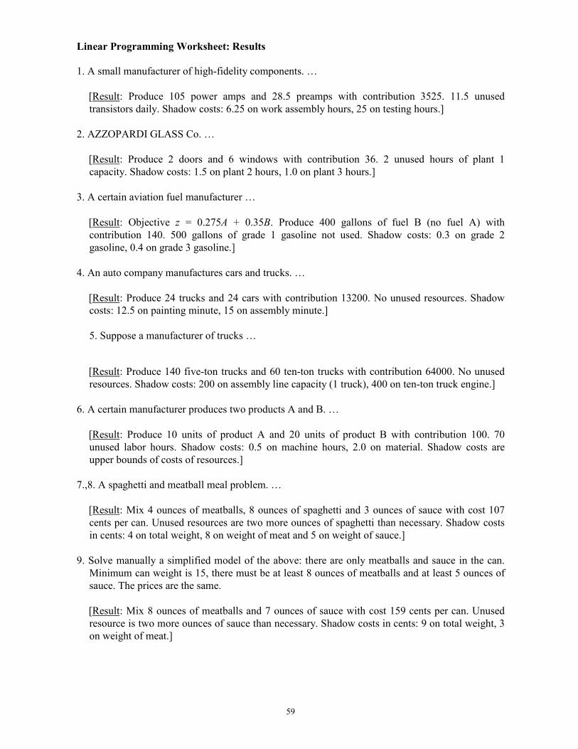
59

Linear Programming Worksheet: Results

1. A small manufacturer of high-fidelity components. …

[Result: Produce 105 power amps and 28.5 preamps with contribution 3525. 11.5 unused

transistors daily. Shadow costs: 6.25 on work assembly hours, 25 on testing hours.]

2. AZZOPARDI GLASS Co. …

[Result: Produce 2 doors and 6 windows with contribution 36. 2 unused hours of plant 1

capacity. Shadow costs: 1.5 on plant 2 hours, 1.0 on plant 3 hours.]

3. A certain aviation fuel manufacturer …

[Result: Objective z = 0.275A + 0.35B. Produce 400 gallons of fuel B (no fuel A) with

contribution 140. 500 gallons of grade 1 gasoline not used. Shadow costs: 0.3 on grade 2

gasoline, 0.4 on grade 3 gasoline.]

4. An auto company manufactures cars and trucks. …

[Result: Produce 24 trucks and 24 cars with contribution 13200. No unused resources. Shadow

costs: 12.5 on painting minute, 15 on assembly minute.]

5. Suppose a manufacturer of trucks …

[Result: Produce 140 five-ton trucks and 60 ten-ton trucks with contribution 64000. No unused

resources. Shadow costs: 200 on assembly line capacity (1 truck), 400 on ten-ton truck engine.]

6. A certain manufacturer produces two products A and B. …

[Result: Produce 10 units of product A and 20 units of product B with contribution 100. 70

unused labor hours. Shadow costs: 0.5 on machine hours, 2.0 on material. Shadow costs are

upper bounds of costs of resources.]

7.,8. A spaghetti and meatball meal problem. …

[Result: Mix 4 ounces of meatballs, 8 ounces of spaghetti and 3 ounces of sauce with cost 107

cents per can. Unused resources are two more ounces of spaghetti than necessary. Shadow costs

in cents: 4 on total weight, 8 on weight of meat and 5 on weight of sauce.]

9. Solve manually a simplified model of the above: there are only meatballs and sauce in the can.

Minimum can weight is 15, there must be at least 8 ounces of meatballs and at least 5 ounces of

sauce. The prices are the same.

[Result: Mix 8 ounces of meatballs and 7 ounces of sauce with cost 159 cents per can. Unused

resource is two more ounces of sauce than necessary. Shadow costs in cents: 9 on total weight, 3

on weight of meat.]

60

Linear Programming Tutorial: Results

1. Ozark Farms. …

[Result: Mix 470.6 lb of corn with 329.4 lb of soybean meal with cost $437.64.]

2. PROTRAC. …

[Result: Produce 4.5 E-9s and 7 F-9s with contribution $50,500.]

3. A pharmaceutical company. …

[Result: Binder 7.64%, disintegrant 2%, filler 76.36%, cost 3.673.]

4. A bank makes four kinds of loans. …

[Result: Mortgage 208.33, home improvement 41.67, 0 to other two, income 37.5.]

5. A wine producer. …

[Result: Table Burgundy 4000, Estate Burgundy 5000, income 67000.]

6. McNaughton Inc, produces two steak sauces …

[Result: Produce only S.D. by mixing 30 quarts of A and 30 quarts of B, income 75.3.]

Assignment Worksheet: Results

1. A1, B4, C3, D2; cost 68

2. A3, B1, C2, D4; profit 73

3. A1, B2, C3, DX; cost 45

4. A2, B1, CX, D3; profit 59

Transportation Worksheet: Note

As the MODI method is not required and completion of the stepping stone iterations is too time-

consuming, use the worksheet as follows:

- find initial basic feasible solutions by all three methods

- perform some stepping-stone iterations on selected non-basic cells.

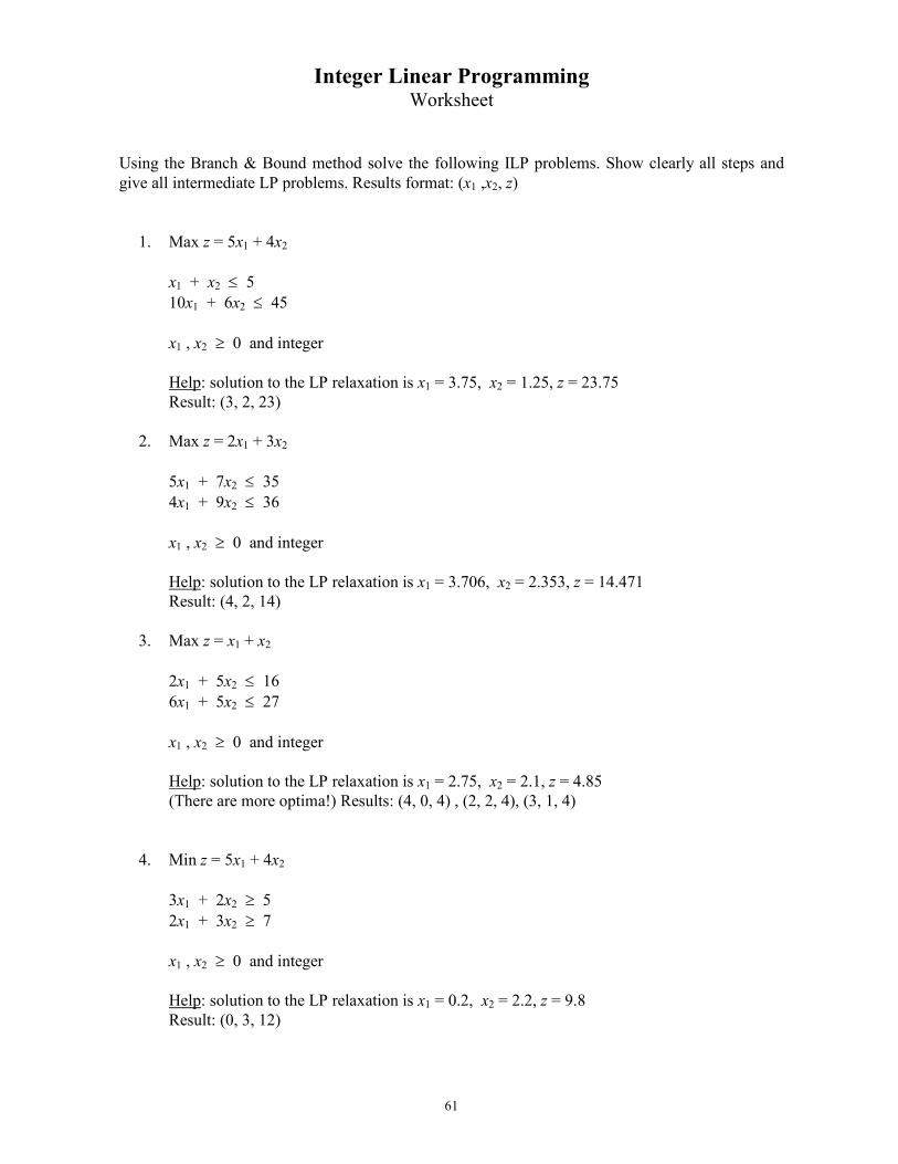
61

Integer Linear Programming Worksheet

Using the Branch & Bound method solve the following ILP problems. Show clearly all steps and

give all intermediate LP problems. Results format: (x1 ,x2, z)

1. Max z = 5x1 + 4x2

x1 + x2 ≤ 5

10x1 + 6x2 ≤ 45

x1 , x2 ≥ 0 and integer

Help: solution to the LP relaxation is x1 = 3.75, x2 = 1.25, z = 23.75

Result: (3, 2, 23)

2. Max z = 2x1 + 3x2

5x1 + 7x2 ≤ 35

4x1 + 9x2 ≤ 36

x1 , x2 ≥ 0 and integer

Help: solution to the LP relaxation is x1 = 3.706, x2 = 2.353, z = 14.471

Result: (4, 2, 14)

3. Max z = x1 + x2

2x1 + 5x2 ≤ 16

6x1 + 5x2 ≤ 27

x1 , x2 ≥ 0 and integer

Help: solution to the LP relaxation is x1 = 2.75, x2 = 2.1, z = 4.85

(There are more optima!) Results: (4, 0, 4) , (2, 2, 4), (3, 1, 4)

4. Min z = 5x1 + 4x2

3x1 + 2x2 ≥ 5

2x1 + 3x2 ≥ 7

x1 , x2 ≥ 0 and integer

Help: solution to the LP relaxation is x1 = 0.2, x2 = 2.2, z = 9.8

Result: (0, 3, 12)

62

Appendix A: The algebra of the Simplex Method

First let's recall the standard form of an LP minimization problem (results for maximization will

mostly differ only in signs and types of inequalities): find such x to

Minimize z = cx

Subject to Ax = b , x ≥ 0

where x and c are n-vectors, b is an m-vector, A is an m x n matrix (m ≤ n) and z is the scalar

objective value. Note that the set of equations Ax = b can be expressed as:

x1a1 + x2a2 + … + xnan = b (1)

where xi are elements of the vector x and ai are columns of the matrix A (1 ≤ i ≤ n ). Note also that

all LP problems can be converted into the above form by elementary operations and by adding

appropriate slack, surplus and artificial variables if necessary.

Now let's assume that the matrix A has the rank m, so there are m independent columns. Then A can

be re-arranged in this way:

A = (B N), where B is an m x m invertible matrix and N is an m x (n-m) matrix.

B is called the basic matrix (shortly the base) of A, N is called the nonbasic matrix. Vector x can be

decomposed accordingly: x = (xB xN) where xB = x1, x2, ... xm and xN = xm+1, xm+2, ... xn. Then:

or (2)

(after multiplying the last equality by B-1 from left). The solution x = (xB, xN) such that xN = 0 and

xB = B-1b is called a basic solution of the system Ax = b. So a basic solution has m basic variables

(components of xB) and n-m zero nonbasic variables (components of xN). If xB ≥ 0, than x is called a

basic feasible solution. If the solution has less than m nonzero variables, it is called a degenerate

basic solution. From the fundamental theorem of linear programming we know that if an LP

problem has an optimal feasible solution, then there is a basic feasible solution that is optimal.

The equation (2) shows how the basic variables would change if the nonbasic variables (currently

all zero) changed their values. Let's express this equation in terms of columns of the matrix B-1N

and corresponding nonbasic variables:

(3)

where R is the index set of the columns that make the nonbasic matrix N, aj are columns of the

matrix N (and the matrix A), yj are columns of the matrix B-1N and b* contains the current values of

basic variables.

Similarly let's find out how would the objective value change with respect to nonbasic variables:

bNxBxx

xNBAx =+=

= NB

N

B)(

NB NxBbBx11 −− −=

j

Rj

jj

Rj

jNB xx ∑∑∈

∗

∈

−−−− −=−=−= ybaBbBNxBbBx )( 1111

63

(4)

where zj = cBB-1aj is a scalar value for each nonbasic variable. We can use the equation (4) to find a

nonbasic variable that (if not zero) would improve the current objective value z0. If such a variable

does not exist, we know that the current basic feasible solution is optimal. To do it, let's optimize

with respect to nonbasic variables at the point x (the origin in the sub-space of nonbasic variables)

using the equations (3) and (4):

Minimize

Subject to

Note that in the above problem the current basic variables play the role of slacks. So the problem

can be rewritten as:

Minimize

Subject to

From the objective function of the above LP problems, we can directly state the optimality

condition:

If (zj - cj) ≤ 0 for all j ∈ R, then the current basic feasible solution is optimal.

The proof is simple: since xj ≥ 0 then for all nonpositive (zj - cj) z ≥ z0 for any other solution. But

currently z = z0 since xj = 0 for all j ∈ R.

If not all (zj - cj) ≤ 0, then we select one positive (zk - ck) - possibly but not necessarily the greatest

one - and we shall increase the corresponding xk as much as possible by holding the remaining n-m-

1 nonbasic variables at zero. The new objective value will be:

z = z0 - (zk - ck) xk (5)

Note: In geometry simplex is defined as an object in Rp defined by (p + 1) non-coplanar points. So

for example simplex in R3 is a tetrahedron. This explains the name "simplex method". At the

beginning of each iteration we are in the origin of the sub-space of nonbasic variables. Each

iteration represents a move along one axis of the nonbasic variables space to the neighboring

corner. So geometrically it is a move on one of the edges of the simplex.

From the equation (3) we can find new values of basic variables:

∑∑∑

∑

∈∈∈

−−

∈

−−

−−=+−=

=+−=+=

==

Rj

jjj

Rj

jj

Rj

jjBB

NN

Rj

jjBNNBB

N

B

NB

xczzxcx

xz

)(

)()(

0

11

11

aBcbBc

xcaBbBcxcxcx

xcccx

∑∈

−−=Rj

jjj xczzz )(0

0xbxy ≥∈≥=+ ∗

∈∑ BjBj

Rj

j Rjxx ,,0,

∑∈

−−=Rj

jjj xczzz )(0

Rjxx jj

Rj

j ∈≥≤ ∗

∈∑ ,0,by

64

xB = b* - ykxk (all other xj , j ∈ R - {k} are zero)

Expanded:

The indices Bi depend on the current basis. The value of xk can be found from the feasibility

requirement of the new solution:

xBi ≥ 0 or bi* - yikxk ≥ 0 , i = 1, 2, ... m

Feasibility is at danger only for positive yik for which it must hold:

So for yik ≤ 0 the corresponding xBi remains nonnegative. For

yik > 0 the corresponding xBi decreases. We can continue increasing xk until the first basic variable

drops to zero. Then we have to stop, otherwise the solution would become infeasible. This gives the

so called feasibility condition also called ratio test:

(6)

If r is the row with the minimum ratio, then the new solution is:

In this way we have reached new (better) basic feasible solution. This process must terminate

(unless there is cycling) because the number of corners (basic feasible solutions) is finite. Cycling

can occur in case of degeneracy and it represents a real problem in computer implementation of the

simplex method. There are method to cope with cycling that are beyond the scope of this material.

Commercial LP packages mostly ignore cycling because cycling prevention would slow down

considerably the computation.

Practical interpretation of (zk - ck)

After entering a so far nonbasic (zero) variable xk into the solution, the new value of the objective

function is:

z = z0 - (zk - ck) xk = cBb* - zkxk + ckxk

k

mk

k

k

mBm

B

B

x

y

y

y

b

b

b

x

x

x

−

=

∗

∗

∗

���

2

1

2

1

2

1

0,,2,1, >=≤∗

ik

ik

ik ymi

y

bx �

>=∗

≤≤0:

1ik

ik

i

mik y

y

bMinx

zero)remain variablesnonbasicother (}{,0

variable)entering the(

) variableleaving the- zerotodrops(,2,1,

kRjx

y

bx

xmiy

bybx

j

rk

r

k

Br

rk

rikiBi

−∈=

=

=−=

∗

∗∗ …

65

So ck = cost of entering one unit of xk

zk = saving caused by entering one unit of xk

That's why (ck - zk) is called reduced cost. We are working with its negative value (zk - ck) because

this is the value in the simplex table - see later. Now let's expand zk :

So cBi = unit cost of the i-th basic variable

yik = amount how the i-th basic variable will decrease

cBi yik = saving caused by decreasing the i-th basic variable

zk = total saving caused by decreasing all basic variables.

Cases of termination

So far we have assumed, that a unique optimal solution has been reached. This is in fact one of three

possible cases (we always assume a feasible problem):

1. zj - cj < 0 , j ∈ R There is a unique optimal solution.

2. zj - cj ≤ 0 , j ∈ R (some zk - ck = 0) There are alternative optima. Entering xk into the solution

would change the basic feasible solution, but not the value z.

3. zj - cj ≤ 0 , j ∈ R (some zk - ck > 0 and yk ≤ 0) The problem is unbounded. All items of the

column yk are non-positive, xk can be increased arbitrarily, so z → -∞.

Simplex Table

To use the simplex algorithm in practice we (and also the computer) need a table that would store

all information needed for tests and operations of the algorithm and that would eventually contain

the optimal solution together with its optimal objective value. Later we shall learn that there will be

in fact even more than that. Let's summarize what we need:

- current basic feasible solution

- current objective value

- information whether the solution is optimal and if not what variable should enter. We know that

for this purpose we need reduced costs of nonbasic variables

- information needed to find the values of entering variables that will also show which variable

leaves the solution. We need, that for that (ratio test) we need columns yj of nonbasic variables

and current basic feasible solution.

By using the equations (2) and (4) the original problem

Minimize z = cx

Subject to Ax = b , x ≥ 0

can be restated as:

∑=

===m

i

ikBi ycz1

kBk

1-

Bk ycaBc

66

Minimize z

Subject to NxN + BxB = b (7)

-cNxN - cBxB + z = 0

To get the current basic solution, we multiply the first equation by B-1 and then by cB from left:

B-1NxN + IxB = B-1

b

cBB-1NxN + cBxB = cBB

-1b (8)

To get the reduced costs, lets add the second equations in (7) and (8):

(cBB-1N - cN )xN + 0xB + z = cBB

-1b (9)

Finally let's express the first equation of (8) and (9) in this unified way, where the first term in (9)

has been replaced by zN - see the equation (4):

B-1NxN + IxB + 0z = B-1

b

(zN - cN )xN + 0xB + 1z = cBB-1b (10)

Note that currently xN = 0, so right hand sides are equal to xB and z respectively. The coefficients of

equations (10) can be stored in a table that has m + 1 rows, and columns corresponding to xN, xB, z

and the right hand sides. We shall label the columns accordingly. For practical reasons we can also

label the rows by the basic variables and by z. This makes a simplex table where BV means basic

variables:

BV xN xB z RHS

xB

B-1N

I

0

B-1b

z zN - cN 0 1 cBB-1b

This table contains all we need to carry out simplex iterations. The second equation of (10) shows

that the z-row contains negative reduced costs.

Notes:

1. Some authors describe a table with positive reduced costs and negative objective value (together

with the coefficient -1 in the z-column). This can be obtained by multiplying the second

equation of (10) by -1.

2. The z-column contains always the same, so it is in fact redundant. That's why it is omitted in

most books.

3. Some authors place the z-row as the first one.

4. The above table has the basic and nonbasic variables grouped together. This can always be done

by re-arranging columns of the table. Doing this after each iteration is time consuming and in

fact useless. That's why it is typical (for manual solution) that the above "nice" form of the table

exists only at the beginning, where the basic variables are slacks and/or artificial variables that

67

we are used to place at the right side in such an order to form directly the unity matrix. Note that

in this case the initial basis is unity: B = B-1 = I, so the initial simplex table contains directly the

coefficients of the constraint equations and the objective function:

BV xN xB z RHS

xB

N

I

0

b

z - cN 0 1 cBb

5. Slacks have zero coefficients in the objective function (cB = 0), so the so called all-slack LP

problems have directly zeros in the z-row in xB columns and also zero in the objective value

(bottom right) entry. So the initial simplex table contains directly the coefficients and no pre-

processing is necessary. If there are artificial variables, the initial table depends on the solution

method. The M-method penalizes artificial variables by a big coefficient M in the objective

function. So to get the initial simplex table it is necessary to perform some elementary matrix

operations to obtain zeros in the z-row in xB columns.

6. Note that after each iteration one basic variable leaves, one nonbasic variable enters. So

assuming we keep the heading labels fixed, after the first iteration one column of the unity

matrix moves to the place of the new basic variable and becomes the column of the variable that

is now nonbasic. After several iterations the columns of the unity matrix are "scattered" in the

table, but all of them are always present. So it is convenient to keep labels of basic variables in

the first (label) column.

7. Each solution has its basis that can be created by taking the appropriate columns of the original

matrix A (indices are the same as the basic variables). Note that at each iteration the table

contains the result of multiplying the original matrix A by B-1. So if there were originally the

unity matrix in A (typically at the right side), there is B-1 now.

Information found in the Simplex Table

In addition to the above requirements, the simplex table contains a lot of useful information:

a) Objective value (z) in terms of nonbasic variables

Apart from zeros in the columns of basic variables the z-row of the simplex table contains the

negative reduced costs. Using reduced costs let's once more express the objective value in terms of

nonbasic variables:

(11)

The rate of change of z as a function of a nonbasic variable xj is:

This is another justification that to minimize z, xj should be increased if cj - zj < 0 or zj - cj > 0

(because this value is stored in the simplex table).

∑∈

−−− −+=−−=Rj

jjjBNNBB xzcz )()( 111 bBcxcNBcbBc

jj

j

zcx

z−=

∂∂

68

b) Basic variables in terms of nonbasic variables

From the equation (10) we get for xB:

(12)

Vectors yj show how basic variables change in terms of nonbasic variables:

c) Objective value (z) in terms of the original right hand side values

From the equation (11) we can compute the partial derivative of z with respect to b:

These values are the so called shadow costs. Their interpretation depends on the type of inequality.

If bi represents availability of a certain resource ( ≤ inequality in a maximization problem) then

∂z/∂bi is the worth of one unit of the particular resource. If bi represents some minimum acceptable

amount ( ≥ inequality in a minimization problem like minimum production, minimum weight and

similar) then the derivative ∂z/∂bi is the cost that we pay for one unit of that limitation. Shadow

costs can also be found in the simplex table (actually for some nonbasic variables shadow costs are

equal to reduced costs). From the equation (9) we know that in the z-row the entries in nonbasic

variables columns are cBB-1N - cN or cBB

-1aj - cj for one particular nonbasic variable xj. Now lets

assume that the nonbasic variable xj is a zero slack of a certain scarce resource whose availability is

bi (i-th component of b). Such slacks have zero coefficients in the objective function, so cj = 0. Also

initially in the simplex table the slack was a basic variable with its associated column of a unity

matrix, so aj = ei (a column vector with i-th component equal to 1 and the remaining components

equal to zero):

cBB-1aj - cj = cBB

-1ei = (cBB

-1)i

Thus the z-row entry of xj is the i-th entry of cBB-1 that is the shadow cost ∂z/∂bi.

d) Basic variables in terms of the original right hand side values

From the equation (12) we can compute the partial derivatives of xB with respect to b:

∑∑∈

−

∈

−−−− −=−=−=Rj

jj

Rj

jjNB xx ybBaBbBNxBbBx11111

ij

j

Bi

j

j

B yx

x

x−=

∂

∂−=

∂

∂,y

x

1−=∂∂

Bcb

B

z

ij

j

BiB

b

x)(, 11 −− =

∂

∂=

∂

∂BB

b

x

69

So the i,j-th entry of B-1 shows how the i-th basic variable (the one in the i-th row, not the one that

is the i-th component of x) changes with the right hand side value bj.

70

Appendix B: Summary of relevant Graph Theory terms

A subnetwork N1 = (V1, A1) of a network N = (V, A) has these properties:

V1 ⊆ V and A1 ⊆ A ∩ (V1× V1)

So a subnetwork (subgraph) is created by removing some vertices, all arcs incident with these

vertices, and possibly some more arcs.

A path from vertex i1 to the vertex ik is a subnetwork consisting of a sequence of vertices i1, i2, … ,

ik, together with a set of distinct arcs connecting each vertex in the sequence to the next. The arcs

need not all point in the same direction.

A network is said to be connected if there is a path between every pair of vertices in the network.

From now we shall assume that the network is connected (if not, the problem can be decomposed

into two or more smaller problems).

A cycle is a path from a vertex to itself.

A tree is a connected subnetwork containing no cycles.

A spanning tree is a tree that includes every vertex in the network.

4. Summary of relevant properties of trees

The properties of (spanning) trees that are relevant for the network simplex method will be given as

lemmas. Let’s recall that our assumption is a connected network without loops.

Lemma 1: Every tree consisting of at least two vertices has at least one end (a vertex that is

incident to exactly one vertex).

Proof: Select any vertex i and follow any path away from it (one must exist because the network is

connected). There are no cycles and the number of vertices is finite, so an end will eventually be

reached.

Lemma 2: A spanning tree for a network with m vertices contains exactly m-1 arcs.

Proof: Lemma can be proved by induction:

1. Lemma in true for m=1 (no arc) and m=2 (one arc).

2. Let’s assume that it holds for any m ≥ 2.

3. Adding one more vertex to the tree means that this vertex will be connected to a vertex of the

current tree with one more arc. So we have a tree with m+1 vertices and m arcs. This

completes the proof.

Lemma 3: If a spanning tree is augmented by adding to it an additional arc of the network, then

exactly one cycle is formed.

Proof: Suppose an arc (i, j) is added to the spanning tree. Since there was already a path between the

vertices i and j, this path together with the arc (i, j) forms a cycle. Suppose that two (or more)

distinct cycles were formed. They all must contain the arc (i, j) because the spanning tree had no

cycles. Then the union of the two (or more) cycles minus the arc (i, j) still contains a cycle, but

this is a contradiction because before adding the arc (i, j) there were no cycles. This shows that

exactly one cycle is formed.

71

Lemma 4: Every connected network contains a spanning tree.

Proof: If the network contains no cycles, then it is also a spanning tree since it is connected and

contains all the vertices. Otherwise, there exists a cycle. Deleting any arc from this cycle results

in a subnetwork that is still connected. This deleting can continue until there are no cycles.

Finally a subnetwork is obtained that contains no cycles, is connected, and contains all the

vertices, so it is a spanning tree.

Lemma 5: Let B be the submatrix of the constraint matrix A corresponding to a spanning tree with

m vertices. Then B can be rearranged to form a full-rank lower-triangular matrix of dimension m

× (m-1) with diagonal entries ±1.

Proof: By Lemma 2 a spanning tree consists of m vertices and m-1 arcs, so B is of dimension m ×

(m-1). The rest can be proved by induction:

1. If m=1 then B is empty. If m=2 then the spanning tree consists of one arc so there are two

possible forms of B that are both of the required form:

1 1or

1 1

− = = −

B B

2. Let’s assume that the Lemma holds for any m ≥ 2.

3. Let’s add one more vertex to the tree. This vertex will be connected to a vertex of the current

tree with one more arc. Let’s assume that in the new matrix the added vertex is in the row 1

and the new arc is in the column 1. Then the new matrix will have the following form:

1±

0

v B

where B is the original matrix. The rest of the row 1 is made of zeros because the newly

added vertex is an end (only the new arc starts or ends in this vertex: ±1 in the first position).

The vector v contains all zeros except ±1 at the position where the new arc is connected to

the tree. If B has the required form then the new matrix has also the required form.

A lower triangular matrix with nonzero diagonal entries has full rank. This completes the proof.

5. Basis of network problems

To show the relationship between a spanning tree and a basis of network problems we need two

more definitions:

Given a spanning tree for a network, a spanning tree solution x is a set of flow values that satisfy

the flow conservation constraints Ax = b for the network, and for which xij = 0 for any arc (i, j) that

is not part of the spanning tree.

A feasible spanning tree solution x is a spanning tree solution that satisfies the nonnegativity

constraints x ≥ 0.

Theorem: A flow x is a basic feasible solution for the network flow constraints

{ x : Ax = b, x ≥ 0 } if and only if it is a feasible spanning tree solution.

72

Proof: First let’s assume that x is a feasible spanning tree solution. Then by Lemma 2 it has mostly

m-1 nonzero components. Let B be the submatrix of A corresponding to the spanning tree. By

Lemma 5, B is full rank with linearly independent m-1 columns, and hence x is a basic feasible

solution.

For the second half of the proof let’s assume that x is a basic feasible solution, so it has mostly

m-1 nonzero components. Now we consider the set of arcs corresponding to the strictly positive

components of x. We shall prove that these arcs do not contain a cycle, so they either form a

spanning tree or they can be augmented with zero-flow arcs to form a spanning tree. To prove it,

let’s assume the opposite that these arcs contain a cycle. In this cycle we can add a small flow ε in one direction (flow in all arc with the same direction will be increased by ε, flow in all arcs

with the opposite direction will be decreased by ε). We can select ε small enough to keep all

flows positive. Let’s call this new flow x+ε. Similarly we can add the same small flow ε in the

opposite direction to get a new flow x-ε. For these two flows we have:

1 1

2 2ε ε+ −= +x x x

But this is a contradiction with the assumption that x is a basic feasible solution (an extreme

point) that cannot be expressed as a convex combination of two distinct points. This completes

the proof.

The constraint matrix A does not have full rank because rows are not linearly independent. That’s

why the basis B has only m-1 columns that correspond to the m-1 arcs of a spanning tree. Lemma 5

gives the properties of a basis that have very important consequence. Let’s suppose that having a

base B we want to compute the values of the basic variables. B has m rows and m-1 columns. We

can remove the last dependent row to get a set of equations:

B’xB = b’

where B’ is obtained from B by deleting the last row, b’ is similarly obtained by deleting the last

component from b, and xB is the (m-1) vector of basic flows. B’ is a square full rank lower

triangular matrix, so the solution can be found by forward substitution. Moreover we know that the

matrix entries Bij are either zeros or ±1. So we know directly the first component x1 of xB:

B11x1 = b1 → x1 = ±b1

Similarly for the second component and so on. Generally we get:

1

1

( ) , 2 1i

i i j

j

x b x i m−

=

= ± − ± = −∑ …

Or in other words xi is computed by adding or subtracting first i components of b. This guarantees

that for integer values of outer flows b the values of basic flows are also integer. This is a natural

requirement of many network problems (like assignment) that is thus automatically satisfied. This is

very important – integer solution is obtained by normal simplex method. There is no need to use a

time consuming integer programming algorithm.

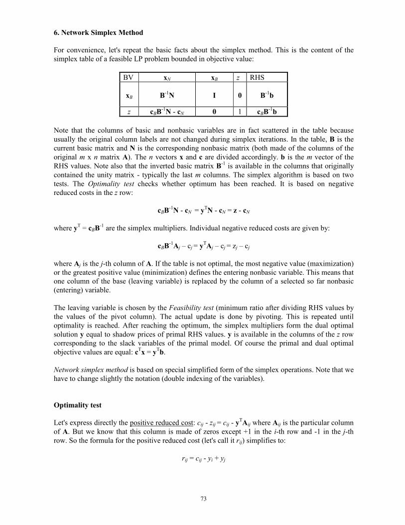
73

6. Network Simplex Method

For convenience, let's repeat the basic facts about the simplex method. This is the content of the

simplex table of a feasible LP problem bounded in objective value:

BV xN xB z RHS

xB

B-1N

I

0

B-1b

z cBB-1N - cN 0 1 cBB

-1b

Note that the columns of basic and nonbasic variables are in fact scattered in the table because

usually the original column labels are not changed during simplex iterations. In the table, B is the

current basic matrix and N is the corresponding nonbasic matrix (both made of the columns of the

original m x n matrix A). The n vectors x and c are divided accordingly. b is the m vector of the

RHS values. Note also that the inverted basic matrix B-1 is available in the columns that originally

contained the unity matrix - typically the last m columns. The simplex algorithm is based on two

tests. The Optimality test checks whether optimum has been reached. It is based on negative

reduced costs in the z row:

cBB-1N - cN = yT

N - cN = z - cN

where yT = cBB-1 are the simplex multipliers. Individual negative reduced costs are given by:

cBB-1Aj – cj = yT

Aj – cj = zj – cj

where Aj is the j-th column of A. If the table is not optimal, the most negative value (maximization)

or the greatest positive value (minimization) defines the entering nonbasic variable. This means that

one column of the base (leaving variable) is replaced by the column of a selected so far nonbasic

(entering) variable.

The leaving variable is chosen by the Feasibility test (minimum ratio after dividing RHS values by

the values of the pivot column). The actual update is done by pivoting. This is repeated until

optimality is reached. After reaching the optimum, the simplex multipliers form the dual optimal

solution y equal to shadow prices of primal RHS values. y is available in the columns of the z row

corresponding to the slack variables of the primal model. Of course the primal and dual optimal

objective values are equal: cTx = y

Tb.

Network simplex method is based on special simplified form of the simplex operations. Note that we

have to change slightly the notation (double indexing of the variables).

Optimality test

Let's express directly the positive reduced cost: cij - zij = cij - yTAij where Aij is the particular column

of A. But we know that this column is made of zeros except +1 in the i-th row and -1 in the j-th

row. So the formula for the positive reduced cost (let's call it rij) simplifies to:

rij = cij - yi + yj

74

To evaluate it we need the simplex multipliers. From the above equations we get yT = cBB-1. After

multiplication by B from right we get yTB = cB. Again, column (i,j) of B is made of zeros except +1

in the i-th row and -1 in the j-th row. So the equations for the simplex multipliers simplify to:

yi - yj = cij for all basic variables xij

This makes m-1 equations for m variables, so one of them can be selected arbitrarily. The others are

then computed and used to compute positive reduced costs for the optimality test. Initially any value

of any variable can be chosen, but to simplify computation it is convenient to assign 0 to a

multiplier that corresponds to an end of the spanning tree. The other values are then computed by

traversing the spanning tree starting from the selected vertex. Initial assignment affects the values of

simplex multipliers but not the values of reduced costs because they are given by differences of the

particular multipliers.

Feasibility test

If the table is not optimal, the optimality test gives the entering variable xij. Using the network

terminology we are adding an arc to a spanning tree by increasing its flow from the current value 0.

Using Lemma 3, this will create exactly one cycle. To keep flow conservation, we have to increase

flow in all arcs of the newly created cycle. Unless the problem is unbounded, some arcs in the cycle

have opposite direction compared with the new arc. So increasing a flow in the cycle will actually

decrease the flow in these arcs with opposite direction. That's why we can increase the cycle flow

until the flow in one (or more) of these arcs drops to zero. Further increase is impossible to keep

feasibility - nonnegative flows. This will also restore the spanning tree because the arc whose flow

has dropped to zero can now be removed. If the flow drops to zero in more arcs, only one of them

can be removed (degeneracy).

We can now summarize the steps of the network simplex method:

1. The optimality test - compute the simplex multipliers y: Start at an end of the spanning tree and

set the associated simplex multiplier to zero. Following the arcs (i, j) of the spanning tree, use the

formula yi - yj = cij to compute the remaining simplex multipliers.

Compute the positive reduced costs. For each nonbasic arc (i, j) compute rij = cij - yi + yj. If rij ≥ 0

(minimization) or rij ≤ 0 (maximization) for all nonbasic arcs, then the current basis is optimal.

Otherwise select the entering arc (i, j).

2. The feasibility test. Identify the cycle created by entering the arc (i, j) to the spanning tree. Find

the arc(s) with opposite orientation compared with the arc (i, j) with minimum flow f. If no such

arcs exist, the flow in the arc (i, j) can be increased arbitrarily and the problem is unbounded.

3. The pivoting. Update the spanning tree. In the cycle subtract f from flows of opposite arcs and add

f to flows of same direction arcs. Remove the arc whose flow dropped to zero (if there are more,

select one arbitrarily).

To find an initial basic feasible solution there are various methods for different forms of network

problems. Generally it is possible to add artificial variables - arcs in such a way that an "obvious"

initial basic feasible solution can easily be found. Then the artificial variables have to be removed

like in the standard simplex method (M-method, II-phase method). For some problems there are

direct methods (like North-West corner method for transportation).

75

Appendix C: Modified Distribution (MODI) method

The MODI method (also called "method of multipliers") improves the search for entering variables.

Using the Duality Theory, it is possible to associate multipliers di with each row and multipliers rj

with each column of the matrix. They can be interpreted as unit dispatch and reception costs

respectively. Then for each basic variable xij the following holds:

di + rj = cij

So we have m+n-1 equations for m+n variables. By selecting any value for one of them (usually

d1=0), the values of the others can easily be computed directly in the table - see the worksheet. The

sum di + rj for nonbasic variables is their shadow cost ad the difference di + rj - cij is the entry in the

z-row of the simplex table. Because the model seeks to minimize the total cost, the presence of a

positive value shows that the solution is not optimal. Enter the variable with the maximum positive

difference, break ties arbitrarily. This difference (shadow cost - actual cost) can be interpreted as

cost saved by transporting one unit of the commodity through this cell.

After selecting the entering variable, the rest is done by creating the loop in the same way as in the

Stepping - Stone method. This will find the leaving variable. This is repeated until there is no

possible improvement. Zero difference (shadow cost - actual cost) indicates alternative optima.

Complete Transportation Algorithm (MODI method)

If (demands < supplies) then add a dummy destination (column) with zero transportation costs and

the demand that makes the balance

If (supplies < demands) then add a dummy source (row) with zero transportation costs and the

supply that makes the balance

Make an Initial basic feasible allocation (all demands must be satisfied, supplies must not be

exceeded). There must be m+n-1 allocations.

Repeat

Calculate dispatch and reception costs in the table by setting the first dispatch cost to zero

Calculate the difference shadow cost - actual cost =

(dispatch cost + reception cost) - actual cost of empty (nonbasic)cells

If (there is a positive difference) then reduce the total cost:

Select the nonbasic cell with maximum difference, break ties arbitrarily

Mark this cell by +

Mark other basic cells by - and + to keep row and column balances

This creates a loop that starts and ends in the selected nonbasic cell

Find the minimum allocation of the cells in the loop marked by -

Add this value to + cells in the loop, subtract this value from - cells in the loop

EndIf

Until (there is no positive difference)

Compute the Total Cost of the optimum solution

76

Transportation - worksheet for MODI method

Destinations: A B C D X

Sources: Demand: 20 30 15 5 10

Supply: D\R

I 40 2

4 1 6 0

II 20 4

3 3 3 0

III 20 1

2 5 2 0

Destinations: A B C D X

Sources: Demand: 20 30 15 5 10

Supply: D\R

I 40 2

4 1 6 0

II 20 4

3 3 3 0

III 20 1

2 5 2 0

Destinations: A B C D X

Sources: Demand: 20 30 15 5 10

Supply: D\R

I 40 2

4 1 6 0

II 20 4

3 3 3 0

III 20 1

2 5 2 0

Destinations: A B C D X

Sources: Demand: 20 30 15 5 10

Supply: D\R

I 40 2

4 1 6 0

II 20 4

3 3 3 0

III 20 1

2 5 2 0

77