Sensitivity method for basis inverse representation in multistage stochastic linear programming...

JOURNAL OF OPTIMIZATION THEORY AND APPLICATIONS: Vol. 74, No, 2, AUGUST 1992

Sensitivity Method for Basis Inverse Representation in Multistage Stochastic Linear Programming Problems'

J . G O N D Z I O 2 A N D A. R U S Z C Z Y l q S K I 3

Communicated by O. L. Mangasarian

Abstract. A version of the simplex method for solving stochastic linear control problems is presented. The method uses a compact basis inverse representation that extensively exploits the original problem data and takes advantage of the supersparse structure of the problem. Computa- tional experience indicates that the method is capable of solving large problems.

Key Words. Linear programming, stochastic programming, simplex method.

I. Introduction

Multistage linear stochastic programming problems are particularly large linear optimization problems which have a specially structured constraint matrix. In this paper, a highly specialized version of the simplex method for such problems is proposed.

Let f~ be a finite probabili ty space with elementary events to and probabilities po,. Next, let the random vectors x~( t ) ~ R", t = O, 1 , . . . , T, u~ ( t ) ~ R m, t = l , 2, . . . , T, and z~ ( t ) c R n, t = l , 2 , . . . , T, denote the state, control, and disturbance of a linear dynamic system, respectively. The problem is to find the sequences of state and control variables (x~,(t) and u~,( t), t = 1, 2 , . . . , T, to c O ) which minimize the linear functional

T

E p,o Z [qr~(t )x ,o( t )+qru(t )u ,o( t )] , (1) w ~ t = l

~This research was supported by Programs CPBP02.15 and RPI.02. 2Assistant Professor, Systems Research Institute, Polish Academy of Sciences, Warsaw, Poland. 3Research Professor, Institute of Automatic Control, Warsaw University of Technology, Warsaw, Poland.

221 0022-3239/92/0800-0221506.50/0 © 1992 Plenum Publishing Corporation

222 JOTA: VOL. 74, NO. 2, AUGUST 1992

subject to the constraints

x,o(t) = Gxo,(t - 1) + Kuo~(t) + z~,(t),

y( t) <- u,o( t) -<- tT(t),

x(t)<- x~(t)<--~(t),

t = l , 2 . . . . . T, ~o 6 l-~,

t = l , 2 , . . . , T, oJ 6 f~,

t = l , 2 , . . . , T, a, 612,

(2)

(3)

(4)

x(0) = Xo, and an additional nonanticipativity constraint, which can be formulated as follows: for each t, the random variables x(t) and u(t) are measurable with respect to the o--subalgebra generated by {z(1), z (2 ) , . . . , z(t)}.

In Eq. (2), G and K denote matrices of appropriate dimensions. The simplifying assumption that G, K, qx, q, do not depend on the time t and the realization w has been introduced only for ease of exposition.

Two important special cases of the above problem are the deterministic control problem (single realizations of x(t) , u(t), z(t) at every stage t) and the two-stage stochastic programming problem (T = 2).

In principle, (1)-(4) is a linear programming problem, but it may have a very large size, because its dimensions grow exponentially with the number of stages T. This limits the application of standard LP approaches (see, e.g., Ref. 1). However, the constraint matrix of (1)-(4) is supersparse, with multiple occurrences of G and K, and has a very special structure. This should be exploited if we want to solve realistic problems.

For the two cases mentioned earlier, a variety of special approaches have been proposed. On the one hand, there are versions of the simplex method with specialized basis inverse representations and pricing strategies (Refs. 2-6). On the other hand, there are decomposition methods that partition (1)-(4) into simpler problems associated with stages or realizations (Refs. 6-11). For general multistage stochastic programs, only decomposition approaches have been suggested so far (Refs. 12-14).

The method presented here aims at exploiting special features of the multistage stochastic problem (1)-(4) within the framework of the classical simplex method. As usually with simplex implementations, the key issue is the way of handling the basis inverse. In general-purpose LP codes, the L U decomposition of Bartels and Golub (Ref. 15) is used (see, e.g., Refs. 16-21). Its heart is the pivot selection procedure which permutes rows and columns of the basis to keep the factors L and U sparse and to ensure numerical stability. Unfortunately, this spreads the fill-in across the whole basis matrix, destroying its structural properties. In particular, the representation of the inverse of a supersparse basis is not supersparse any more. This limits the method's capability of solving problems of form (1)-(4).

The approach discussed in this paper preserves supersparsity by specializing the ideas of basis partitioning and augmentation to the multi-

JOTA: VOL. 74, NO. 2, AUGUST 1992 223

stage stochastic problem. Generally, methods of this type distinguish some convenient (easily invertible) form of the basis, and they try to represent general bases in terms of this form and some additional data. Fundamental concepts associated with this class of methods were extensively discussed in Ref. 22 in which a product form of the inverse was used to pass from the easily invertible basis to the current basis. Similar ideas were further developed in Refs. 5 and 23.

Our approach is closely related to the method suggested in Ref. 2 for deterministic dynamic programs. Bisschop and Meeraus decompose the current basis into Bartels-Golub L U factors and, at later iterations, use Schur complements rather than standard updates. This limits the growth of the fill-in of the inverse representation in successive iterations. The size of the Schur complement is bounded by the refactorization frequency. Unfortu- nately, for multistage stochastic programs, this is not sufficient because of the enormous size of the current basis and its L U factors. Therefore, instead of using a basis from the past, we look for such a triangular fundamental basis in the constraint matrix that has as much in common with the current basis as possible. This fundamental basis needs no extra storage (pointers to the selected columns of the original constraint matrix suffice) and equations with it can be solved elementarily. Together with a Schur complement of hopefully small size, it represents the current basis. The space required by the basis inverse representation is thus solely determined by the size of the Schur complement. At later iterations, the Schur complement grows, so we update the fundamental basis from time to time. It turns out that, for multistage stochastic programs, this approach gives significant savings.

The Schur complement [which we call the sensitivity matrix due to its interpretation for (1)-(4)] is in general dense and small. Equations involving the basis matrix can be replaced by a sequence of equations with the fundamental basis and the sensitivity matrix. Updating the representation of the basis inverse (after column exchange in the basis) resolves itself to changes in the sensitivity matrix alone. We may note here that the idea of using Schur complements in large-scale LP methods has recently been mentioned also in Ref. 24. In Refs. 25 and 26, advantages of using Schur complements in interior-point methods are reported.

The paper is organized as follows. In Section 2, we reformulate (1)-(4) in a tree-like form; then, we introduce the initial fundamental basis and show its main properties. In Section 3, we define the sensitivity matrix and we show how to solve equations with a modified basis. We devote Section 4 to the problem of updating the basis inverse representation and Section 5 to refactorization. In Section 6, we present numerical results and analyze the practical efficiency of the method. Finally, we have a conclusion section.


2. Fundamental Basis

It is convenient to reformulate multistage stochastic programs in a tree-like form. With the set of disturbance realizations (scenarios) z,~(t), t = 1, 2 , . . . , T, we can associate a tree i f with node set J defined as follows. There is one root node i0 at level 0. At level 1, there are as many nodes i e J1 as different realizations of z~ (1) may occur. They all have i0 as their father (predecessor). Generally, each node i ~ Jt at level t corresponds to a different realization of {z(1), z ( 2 ) , . . . , z(t)}. Nodes j c Jt+l are joined with i e J, if the realization corresponding to j is a continuation of the realization associated with i.

Each node at level t corresponds to the information available at time t. The requirement of nonanticipativity of controls (which implies nonanticipativity of state trajectories) makes it possible to associate decisions with nodes and reformulate our problem as follows: Find u(i) and x( i ) , i e J, so as to minimize

Y~ [q~( i )x ( i )+ q~(i)u( i )] , (5)

subject to the constraints

x( i ) = G x ( f ( i ) ) + K u ( i ) + z ( i ) , i t J, (6)

x ( i ) < ~ x ( i ) ~ 2 ( i ) , i~J , (7)

u(i)<-_u(i)<-~(i), i~J . (8)

Here, f ( / ) denotes the father of node i, x(io) = Xo, and _x(i), ~(i), _u(i), a( i) , q~,(i), qu(i) follow directly from (2)-(4).

Thus, the problem is fully defined by the structure of ~, the vectors z(i) , _x(i), Y(i) , _u(i), a(i) , qx(i), qu(i) associated with the nodes of ~-, and the two matrices G and K. The storage requirements necessary to represent the problem in this fo rm are very modest.

From a theoretical point of view, we can consider (5)-(8) as a linear programming problem

min c~x + r Cu U,

s.t. Box + Nou = b,

where

x ~ x ~

~ u ~

x = x ( J ) , u = u ( J ) ,

N o u = K u ( J ) , b = z U ) ,

.u = u_(J), a = a ( J ) .

BoX = x ( 1 ) - G x ( f ( J ) ),

_x =_xU) , ~ =~z(J) ,

(9) (10) (11) (12)

JOTA: VOL 74, NO. 2, AUGUST 1992 225

The constraint matrix of (10),

A = [Bo, No], (13)

may be of enormous size, but has a very special structure, with multiple occurrences of the matrices G, K and the identity matrix L It is clear that any column of A can be easily reconstructed from (6); a very efficient technique of double addressing to columns of G and K can be used to save space.

The factorization of the basis matrix is the key computational problem in any implementation of the simplex method. The matrix (13) is very sparse, so each basis is very sparse, too, and a good factorization technique (of., e.g., Refs. 16-18 and 20) can be quite effective here. However, there is one important feature which is not used by general basis management packages: the block-tree structure and the multiple occurrences of columns of G, K, I in the basis. We have to take advantage of that if we want to go beyond the s~ze admitted by standard factorization methods.

There exists a special basis in (9)-(12) for which inversion is trivial: the matrix Bo. Indeed, suppose that all the state variables x(i) , i e J, are basic and the controls u(i), i ~ J, are nonbasic variables. Then, the equation

Box= b (14)

can be solved by direct simulation of the state equations (6) starting at the root and ending at leaves,

x( i) = Gx ( f ( i) ) + b( i), i ~ J, (15)

where x(io)= Xo. Similarly, the transpose system

T rt TBo = c~ (16)

can be solved by simulating in the reverse direction (from the leaves to the root) the adjoint equations

¢rr(i) = E ¢rr ( j )G+c~( i ) , i~J , (17) jEN(i)

where N( i ) is the set of sons of node/,

N( i ) ={j: i = f ( j ) } .

To verify (17), let us consider the scalar product 7rrBox. We shall show that it is equal to c f x for all x if and only if (17) is fulfilled. Setting b = Box,

226 JOTA: VOL 74, NO. 2, AUGUST 1992

from (15) we get

7 r r B o x - c~x = ¢rTb -- C~x = • I rT( i )b( i ) -- c~x i~J

z,'Y ( i)[ (x ( i) - G x ( f ( i) ) ] - c~x =~

= ~ 7rT(i )x( i ) - Y. 7 r T ( i ) O x ( f ( i ) ) - - C ~ X i ~J i c J

= ~ ~'r(i)x( i ) - E ~. ~T(j)Gx(i) - E cT( i )x ( i ) i c J iEJ j E N ( i ) i c J

i ~ J j e N ( i )

Since T

7'i" T n o ~ Cx ,

then the right-hand side of the above expression must be zero for any x, which proves (17).

Consequently, Eqs. (14) and (16) can be solved very efficiently with no additional storage. Although the matrix Bo composed of the columns associated with state variables has additional advantages and interesting interpretations, any triangular submatrix of A would do as well. In fact, we are going to redefine Bo occasionally.

3. Modified Bases and Sensitivity Matrix

In the previous section, we saw that equations with the fundamental basis and its transpose can be solved by substitution. In general, however, we shall have to deal with bases having columns corresponding to both types of structural variables: states and controls. Each such basis matrix, after necessary column permutations, can be expressed in the form

B =[BOB, No~], (18)

where BoB is a certain submatrix of B0 and Non is a submatrix of No. For further discussion, we shall use a notation referring to partition of

vectors and matrices for basic and nonbasic parts,

x=(x~,xN), u=(uB, uN),

Cx=(CxB, CxN), C~=(C~,~,,C~,N),

Bo = [BOB, BON], No = [NOB, NON]-

For example, NoN is the part of No that remained in iV, etc.


Let V denote a 0-1 matrix of dimension I x M, where I is the number of columns of NoR and M is the dimension of the basis B. Each row of V contains one at the position corresponding to the column of Bo replaced by a column of No. Such definition implies the following relations

B V T = NoR, BoV T = BoN,

so that the exchange of BoN to NoR in the basis can be formalized as follows:

B = Bo+ (NoR - BoV T) V. (19)

It has been observed (Ref. 27) that, instead of working with a basis of form (19), we can work with a larger matrix,

0 - - •

Equations with B~ ug can be solved with the application of the Schur complement

S = VBolNoB ; (20)

see, e.g., Ref. 28. Under the additional condition that Bo is triangular and (as a submatrix of A) is already available, this approach leads to substantial memory savings.

The elements of S have the form

where

s o = viBoluj,

v~=(0 , . . . ,0 , 1,0 . . . . ,0)

is the ith row of the matrix V and u s is the jth column of NoB, i.e., a certain column of No appearing in the basis. The vector v, has a one at the pth position if the pth column of Bo does not appear in B. Consequently, S~k is the sensitivity of the state variable corresponding to the pth column of Bo with respect to the control variable corresponding to the j th column of NoR. For this reason, we call S the sensitivity matrix. S is a square nonsingular submatrix of the full sensitivity matrix

So = Bol No,

but we assume that the size of S is much smaller than the size of So (which is enormous), and we shall rather compute elements of S only when necessary, instead of calculating So in advance.


We can easily find the general form of the entries of S using the tree model (6) and their interpretation as sensitivities. Let the ith row of S correspond to Xk(n) and the j th column of S correspond to ul(m), where n and m are some nodes of 9-. I f m is on the path from n to the root, then

s o = (G~'K)kt , (21)

where 8t is the number of stages between n and m. If the path from n to the root does not include m, we have s o = 0.

Let us now recall some elementary properties of the Schur complements, giving their interpretation for our problem.

Proposition 3.1. The sensitivity matrix (20) is nonsingular.

Proof. Since B0 and B are nonsingular, the rows of B o l B are linearly independent, and so are the rows of VBoIB = SV. []

The main advantage of the Schur complements is that equations with the basis matrix (19),

Bd = a, (22)

B ~ = ca, (23)

can be replaced by sequences of simpler equations with the fundamental basis Bo and with the sensitivity matrix S. These general relations (see, e.g., Ref. 28) can be rewritten in our case as follows.

In (22), the vector d can be partitioned into two parts, d = [dx~, dun], where the components d~B correspond to the columns of B which are in common with Bo and dub corresponds to columns of B coming from No.

Proposition 3.2. The unique solution of Eq. (22) can be obtained by solving the following sequence of equations:

Bodx = a, (24)

Sdo. = v~x, (25)

Bod~ = a - Nond~B, (26)

d = dx + VTd, B. (27)

Proof. Equations (18) and (22) yield

BoBdx8 + NoBd, B =- a,


T T which can be rewritten in the form (26), provided that d r = [dxs, d~N] has d~N = 0. Substituting dx from (26) into dxN = Vdx = 0, we obtain

V B o ~ ( a - NoBd, ,~) = O,

and further, by (20),

S d , B = VB~ t a,

which is equivalent to (24)-(25). Finally, (27) just puts dua in place of dxN = 0 in d~. Uniqueness of d results from the nonsingularity of B. []

Thus, we have to solve two equations with Bo and one equation with the sensitivity matrix S, whose dimension is equal to the number of new columns in B.

Let us now pass on to the dual equation (23). Analogously to Proposi- tion 3.2, we have the following result.

Proposition 3.3. The unique solution of Eq. (23) can be obtained by solving the following sequence of equations:

~7-Bo = 7- cx, (28)

o7-S= c,sr - ~rT-Nos, (29)

7r TBo = c~ + o T-V. (30)

Proof. Setting

CB T 7- T = [cx~, c,,s],

we can use (18) to transform (23) to the following two equations:

7T 7-BOB - - T - cxB, (31)

~r 7-No B 7- = cut~- (32)

Let us now define a vector o by

o T 7rTBoN T = - c~N. (33)

The definition of V and Eqs. (31) and (33) imply (30). Solution of Eqs. (31)-(32) needs then finding such o that the solution rr of (30) satisfies (32). This yields

7- - ( c ~ + v T-V)Bo~No~ T -~ = c ~ B o NoB+vT-S , CuB

which is equivalent to (28) and (29). Again, the nonsingularity of B ensures the uniqueness of ~-. []


Consequently, (23) has been replaced by two equations with Bo r and an equation with the sensitivity matrix (20). In fact, (28) does not depend on B at all and need be solved only once.

Summing up, equations with modified bases and their transposes can be replaced by equations with the fundamental basis and with the sensitivity matrix S. Equations with the fundamental basis resolve themselves to simple substitution, so it remains to develop a method for dealing with (25) and (29).

4. Updating Basis Inverse Representation

In this section, we show that updating the basis inverse representation in successive iterations of the simplex method causes changes only in the sensitivity matrix. Since the fundamental basis Bo does not need any additional storage, the memory requirements of the method are limited to the room for inverse representation of the sensitivity matrix, which in turn may be kept within reasonable limits.

Successive iterations of the simplex method cause specific transformations of S. Four cases may occur, depending on the type of columns that leave and enter the basis. Let us analyze them in detail.

Case 1. A column aj from No replaces a column ai from Bo. The new sensitivity matrix S' is now defined by

e T ' r T /7" '

where e~ c R ~4 is the unit vector with one on its ith position,

s = VBotaj, r "r =eir Bo-1 NOB, cr = e fBo la j .

The v e c t o r Bolaj has already been computed to determine the leaving column [see (24)], so the main cost of this update is the pricing 7rrNoB with ~r r = e f B o l to find r r. In this case, a new column and a new row are added to S.

Case 2. A column a~ from No replaces another column ai from No. Assume that ai was on the pth position in NoB. We then have

N~B = No~ + ( aj -- a , ) e l , V ' = V, S ' = S + de l ,

where ep c l~ 1 is the unit vector with one on its pth position and d = V B o l ( a j - a~). Thus, the pth column of S is changed to

s = VBolaj,

where, as in Case 1, the vector Bolaj is already known.


Case 3. A column aj of Bo replaces a column ai of B0. Let p be the number of the row of V that removes aj from the basis (i.e., it contains one at the j th position). We have

N'oB= No~, V ' = V+ep(e~-es ) T S ' = S + e p d r,

where ep ~ R 1, e~, ej ~ R M are appropriate unit vectors, p is the index of the row corresponding to a~, and

d T = (e, - ej)TBolNoB.

Thus, the pth row of S is replaced by

r r = eTBolNoB.

Case 4. A column aj of Bo replaces a column a~ from No. Let p be the row number in V corresponding to aj, and let q be the column index in No~ corresponding to a~. Then, V' is equal to V with the pth row deleted, N~n equals NOB without the qth column, and S' can be obtained by deleting the pth row and the qth column of S.

The necessity to solve Eqs. (25) and (29) at each iteration of the simplex method creates the need for factorization of the sensitivity matrix. There are two issues that should be taken into account in this respect: numerical stability and the possibility of updating the factors when S is modified.

S is a computed matrix, so it may contain numerical errors. Addi- tionally, S is potentially ill-conditioned [see Eq. (21)]. This suggests the use of the highly stable QR factorization approach (see, e.g., Ref. 29), as proposed in Ref. 27. Its main disadvantages are storage requirements (an l x l matrix Q and a triangular l x l matrix R have to be stored) and time-consuming updates. The L U factorization is clearly more economical, but we need here carefully designed updating procedures to avoid excessive propagation of round-off errors. Two efficient methods of L U factorization (Refs. 15 and 30) proved to be stable enough for practical applications, although counterexamples for their good behavior are given in Refl 21. Their specialized implementations (Refs. 18 and 30) do not offer possibilities of updating the factorization in all four cases analyzed earlier. Such possibility exists in a method described in Ref. 20, where sparse L U decomposition is analyzed, but we need a dense factorization with more stress on stability.

We suggest to represent the sensitivity matrix in the form

S = PLUQ, (34)

where L is a unit lower triangular matrix, U is upper triangular, and P and Q are row and column permutation matrices, respectively. The choice of permutations is mainly conditioned by the need of maintaining good stability properties. Such a dense L U decomposition was analyzed in detail in Refs. 31 and 32. The method extends the one of Ref. 30 to allow stable updating


of the triangular factors of the sensitivity matrix in all four cases: row and column addition or deletion and row or column exchange.

Summing up, the main feature of our basis handling is that we reduce the size of the inverse representation substantially, but we pay for that with double solutions of equations with the fundamental basis (see Propositions 3.2 and 3.3) and with more involved factorization schemes for the sensitivity matrix.

5. Refactorization

The storage requirements of the method are practically limited to the memory needed for the inverse representation of the sensitivity matrix. It is then important to force S to be as small as possible. The iterations of the simplex method may, however, cause fast growth of its dimension (if Case 1 update often occurs). Accumulation of round-off errors is also inevitable. A natural way of preventing it is to redefine the fundamental basis and to recalculate S.

As usual with factorization schemes, two criteria should be taken into account when looking for a new fundamental basis Bo: storage economy and numerical stability.

The block-tree structure of our problem and its large size imply that every basis matrix will be nearly triangular (subject to row and column permutations) with a small number of spikes: columns that disturb triangularity. To save storage, we would have to choose permutations in such a way that the number of spikes is as small as possible, because this determines the size of S. On the other hand, we have to solve equations with Bo (see Propositions 3.2 and 3.3) and, which is even more important, the sensitivity matrix S is defined by Bo ~. Ill-conditioning of Bo would cause errors in the computation of the elements of S and, consequently, errors in solving the equations with the basis matrix. The need to keep the condition index of Bo within reasonable limits imposes additional conditions on the choice of permutations.

Redefinition of the fundamental basis is done in the following two steps:

(i) permute rows and columns of the current basis matrix so as to minimize the number of spikes under additional stability criteria;

(ii) replace spike columns by slack columns to restore the triangularity of the fundamental basis [all spike columns define the new matrix No~; see Eq. (18)].

For Step (i), the p5 method suggested in Ref. 33 appears to be most suitable. It is an improved version of Hellerman's and Rariek's (Ref. 34)


p3 method (preassigned pivot procedure). We can mention here that con- trolling stability in the Bartels-Golub factorization when p3 or pS are used is difficult, because small pivots or even structural zeros may occur in the numerical phase of the factorization. In our approach, after p5 all spikes are removed from the basis, so its stability is determined by the diagonal elements in the triangular part only. The spikes NoB define S by (20), but their order is not important for stability, because when factorizing S by (34) we allow additional row and column permutations.

By imposing conditions on the diagonal elements of B0, we can guaran- tee good numerical accuracy of the equations with it and we can control errors in the elements of S. It is sufficient to require that the diagonal elements bjj of Bo satisfy the following inequalities:

tb~[>-tz max tb01, j = l , 2 . . . . ,M, (35)

where ~ is a prescribed threshold from the interval (0, 1]. So, the stability of the whole sensitivity method is practically conditioned only by the stability of the factorization of S (see Propositions 3.2 and 3.3).

If condition (35) is strong (/~ is near to one), it may significantly affect Step (i) of the fundamental basis redefinition. In such a situation, the number of spikes may increase because of a large number of columns rejected for small diagonal elements. This would cause growth of the dimension of S and also significant decrease of its density. Dense LU factorization of Ref. 32, applied for inverse representation of the sensitivity matrix, could then be replaced with the method of Ref. 20.

6. Numerical Experience

The sensitivity method has been implemented on an IBM PC/AT computer with 10 MHz 80287 coprocessor, 640 kB memory available, and relative precision e = 2.2 × 10 -~6.

Two classes of multistage linear programs were solved. The first group was derived from a simplified flood control problem for the system of reservoirs in the Upper Vistula Region (Fig. 1).

Three reservoirs (R1, R2, R3) really exist; six smaller reservoirs are introduced to model wave transformation in the river. The dynamics of the ith reservoir, i = I, 2 , . . . , 9, is described by the equation

x~(t)=x~(t-1)-u,( t)-v~(t)+d,( t) , t= 1 , 2 , . . . , T, (36)

where x~(t), ui(t) + v~(t), and di(t) denote state, control (i.e., release), and inflow at stage t, respectively.


~ 7

d

Fig. 1. Reservoirs in Upper Vistula Region.

The control is divided into two parts: the admissible release u~(t), bounded above by ai; and the overflow vi(t) that causes flood. State and control must satisfy the following inequalities:

O<-x(t)~Y~, O<--u(t)<--~, 0~ v(t), t = l , 2 , . . . , T. (37)

For simplicity of the model, only the three largest external inflows are taken into account: dl, d2, d3 (see Fig. 1).

Our aim is to find such a nonanticipative policy u(t), v(t), t= 0, 1 , . . . , T, satisfying (36) and (37) that minimizes the expected loss caused by flood,

T E • [wry(t)], (38)

t=0

where E denotes the expected value and w is the vector of loss coefficients defined for the river parts below every reservoir. A number of problems of type (36)-(38) were solved. Depending on the discretization step, the number of stages varied from 3 to 100. The problems were deterministic or stochastic, which is indicated by the letters D or S in their names. Two possible wave transformation models were applied: a simple delay model and the Muskin- gum model of Ref. 35; see the letters DL or MSK in the problem names. All the problems are listed in Table 1. The naming convention is such that SFL10DL is the stochastic flood control problem with 10 stages and with the delay model of wave transformation, DFL20MSK is the deterministic flood control problem with 20 stages and the Muskingum model, etc.

The second class of test problems was randomly generated. We call them SRGi. They are also listed in Table 1.

Table 1 contains the problem name, the dimension of the state vector n, the dimension of the control vector m, the number of stages T, the number of constraints M, the number of variables (including slacks)/'4, the number

JOTA: VOL 74, NO. 2, AUGUST 1992

Table 1. Test problems,

235

Problem n m T M N NZ Density (%)

DFL3DL 9 18 3 27 117 183 5.80 DFL3MSK 15 18 3 45 159 339 4.75 DFL6DL0 9 18 6 54 225 366 3.01 DFL6DL1 9 18 6 54 225 366 3.01 DFL6DL2 9 18 6 54 225 366 3.01 DFL10DL0 9 18 10 90 369 610 1.83 DFL10DL1 9 18 10 90 369 610 1.83 DFL10DL2 9 18 10 90 369 610 1.83 DFL20MSK 15 18 20 300 975 2260 0.77 DFL25DL 9 18 25 225 909 1525 0.74 DFL50MSK 15 18 50 750 2415 5650 0,31 DFLI00DL 9 18 100 900 3609 6100 0,19

SFL6DL 9 18 6 567 2277 3843 0.30 SFL10DL1 9 18 10 558 2241 3782 0,30 SFL10DL2 9 18 10 837 3357 5673 0.20

SRG1 3 2 2 27 75 162 8.00 SRG2 3 2 3 81 219 486 2.73 SRG3 3 2 4 351 939 2106 0.64 SRG4 3 2 7 762 2035 3810 0,25 SRG5 12 3 4 360 822 5670 1,92 SRG6 12 3 5 744 1686 4588 0,37 SRG7 3 2 5 891 2379 4752 0.22 SRG8 12 8 5 1128 3020 20304 0,61 SRG9 3 2 5 891 2379 4752 0,22 SRG10 12 3 5 744 1686 11718 0,94 SRGll 12 3 5 1128 2550 17766 0.62 SRG12 12 8 5 1128 3020 23406 0.69

o f nonze ro e lements o f the const ra int matr ix (exc luding objec t ive and

r igh t -hand-s ide vectors) N Z , and the densi ty o f the const ra in t matr ix,

Three me thods were used to solve the problems.

Standard Simplex Method. The X M P package o f Mars ten (Ref. 36)

wi th special p rob l em data hand l ing that exploi ts the superspars i ty o f the

const ra in t mat r ix was appl ied . LA05 rout ines (Ref. 18) imp lemen t ing the

B a r t e l s - G o l u b L U upda tes were used to represent the basis inverse. Pivot

to le rance was set to ¢v = 10-6, and the th resho ld va lue o f the entries in the

B a r t e l s - G o l u b e lementa ry opera tors w a s / z = 0.1. Refac to r iza t ion was per-

fo rmed every 50 i terat ions. The starting basis was cons t ruc ted f rom slacks.

A combina t i on o f par t ia l and mul t ip le pr ic ing strategy was used when

select ing a var iable to enter the basis.


Specialized Simplex Method. The method differs from the previous one only in the starting basis selection and the pricing rule. A crash basis constructed from the state variables leading to the basis matrix Bo defined by Eq. (10) was used. A progressive pricing rule (Refs. 31 and 37) that exploits similarities between variables associated with successive time stages or different realizations at a given stage was applied.

Sensitivity Simplex Method. Within the specialized simplex method, the sensitivity method was used for basis inverse management instead of the Bartels-Golub LU updates. Refactorization was performed every 50 iterations. Stability criterion (35) with /x = 0.01 was used when searching for a fundamental basis. The dimension of the sensitivity matrix was limited to 80.

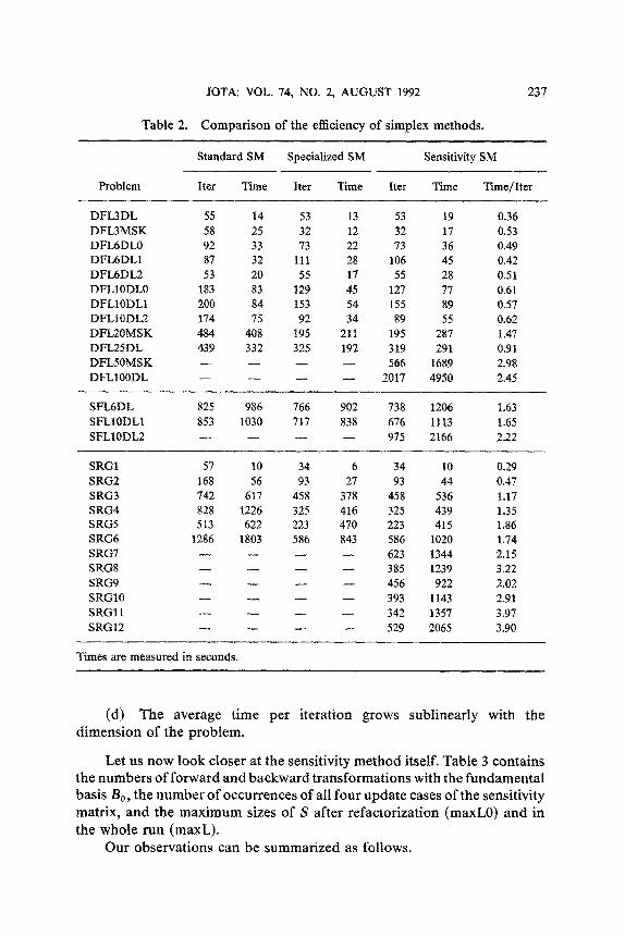
Table 2 collects information (number of iterations and computation time) on the performance of all three methods described above for all test problems. The last column contains the average time of one iteration of the sensitivity method. Empty fields in Table 2 mean that the problem was too large to be solved by a given method.

The results can be summarized as follows.

(a) The sensitivity representation of the basis inverse requires very small memory, which allows solving significantly larger problems. The memory space needed is almost independent of the number of nonzero elements in the constraint matrix. Real limits of application of our method result from the necessity of storing several long vectors such as cost coefficients, lower and upper bounds of the variables, primal and dual variables, right-hand sides, etc.

(b) For medium-size problems (M-> 200) for which all methods suc- ceeded, the sensitivity simplex method is about 30% slower than the specialized simplex method. The main reason for that is the indirect access to the data while solving equations with the basis matrix.

(c) In Phase 1 of the simplex method, the sensitivity method is about 40-50% slower, while in Phase 2 it is about 5-10% slower than the specialized simplex method. This is due to the possibility of storing partial results of the backward transformation [i.e., the solution ~ of Eq. (28)]. Such savings in Phase 1 are not possible, because the objective changes at every iteration. In randomly generated problems SRGi, the starting bases constructed entirely of state variables were feasible, so only Phase 2 iterations were performed. On the contrary, in flood control problems such starting bases were far from being feasible. In these problems, about 70-90% iterations were spent in Phase 1. That is why the ratio of computation times in sensitivity and specialized simplex methods is for these problems larger.

JOTA: VOL. 74, NO. 2, AUGUST 1992

Table 2. Comparison of the efficiency of simplex methods.

237

Standard SM Specialized SM Sensitivity SM

Problem Iter Time Iter Time Iter Time Time/Iter

DFL3DL 55 14 53 13 53 19 0.36 DFL3MSK 58 25 32 12 32 17 0.53 DFL6DL0 92 33 73 22 73 36 0.49 DFL6DL1 87 32 111 28 106 45 0.42 DFL6DL2 53 20 55 17 55 28 0.51 DFL10DL0 183 83 129 45 127 77 0.61 DFL10DL1 200 84 153 54 155 89 0.57 DFL10DL2 174 75 92 34 89 55 0.62 DFL20MSK 484 408 195 211 195 287 1.47 DFL25DL 439 332 325 192 319 291 0,91 DFL50MSK . . . . 566 1689 2.98 DFL100DL . . . . 2017 4950 2,45

SFL6DL 825 986 766 902 738 1206 t.63 SFL10DLI 853 1030 717 838 676 1113 1.65 SFL10DL2 . . . . 975 2166 2.22

SRG1 57 10 34 6 34 10 0.29 SRG2 168 56 93 27 93 44 0.47 SRG3 742 617 458 378 458 536 1.17 SRG4 828 1226 325 416 325 439 1.35 SRG5 513 622 223 470 223 415 1.86 SRG6 1286 1803 586 843 586 1020 1.74 SRG7 . . . . 623 1344 2.15 SRG8 . . . . 385 1239 3.22 SRG9 . . . . 456 922 2,02 SRG10 . . . . 393 1143 2.91 SRG11 . . . . 342 1357 3.97 SRG12 . . . . 529 2065 3,90

Times are measured in seconds.

(d) The average time per iteration grows sublinearly with the dimension of the problem.

Let us now look closer at the sensitivity method itself. Table 3 contains the numbers of forward and backward transformations with the fundamental basis Bo, the number of occurrences of all four update cases of the sensitivity matrix, and the maximum sizes of S after refactorization (maxL0) and in the whole run (maxL).

Our observations can be summarized as follows.


Table 3. Sensitivity method statistics.

Equations with B o Updates Size of S

Problem FT BT Case 1 Case 2 Case3 Case 4 maxL0 maxL

DFL3DL 107 111 27 13 1 3 0 24 DFL3MSK 65 84 24 5 2 0 0 24 DFL6DL0 145 172 48 18 1 0 0 35 DFL6DL1 213 216 58 22 2 4 0 35 DFL6DL2 111 131 35 16 1 I 0 34 DFL10DL0 253 307 95 6 6 3 0 48 DFL10DL1 311 356 104 16 0 4 0 46 DFL10DL2 179 231 75 9 0 1 0 45 DFL20MSK 397 514 153 27 0 2 1 52 DFL25DL 637 782 257 18 1 4 0 51 DFL50MSK 1190 1440 448 32 4 3 36 70 DFL100DL 4034 4636 1159 697 3 27 0 51

SFL6DL 1475 1883 598 36 10 4 0 51 SFL10DL1 1349 1782 544 29 8 2 0 51 SFL10DL2 1949 2517 828 31 10 2 0 51

SRG1 69 53 20 12 0 0 0 20 SRG2 192 166 73 16 0 2 3 27 SRG3 1023 827 381 52 2 0 17 62 SRG4 650 402 202 0 0 0 0 51 SRG5 542 409 177 35 5 5 29 71 SRG6 1202 913 447 10 1 0 4 55 SRG7 1354 1207 572 t8 15 10 17 60 SRG8 810 642 285 49 4 8 9 54 SRG9 753 711 349 14 0 1 4 55 SRG10 940 696 282 94 14 3 29 70 SRGIt 787 644 283 36 12 11 16 64 SRG12 1318 985 421 66 26 14 38 77

(e) T h e r a t io o f b a c k w a r d a n d f o r w a r d t r a n s f o r m a t i o n s o f Bo fo r

f l ood c o n t r o l p r o b l e m s is l a rge r t h a n fo r the r a n d o m l y g e n e r a t e d o n e s [ f l ood

c o n t r o l p r o b l e m s n e e d m a n y i t e ra t ions to f ind a f eas ib l e s o l u t i o n - - s e e

i ssue (c)] .

( f ) C a s e s 1 a n d 2 o f t h e sens i t iv i ty m a t r i x u p d a t e s a re m o s t f r e q u e n t .

I n fac t , r e s t r i c t ing the t r a n s f o r m a t i o n s o f S to t he first two cases o n l y (i.e.,

t r e a t i n g c o l u m n s o f Bo t h a t lef t t he bas is a n d en t e r it aga in as n e w o n e s )

w o u l d n o t c a u s e s ign i f i can t c h a n g e s in the e f f ic iency w h i l e s i m p l i f y i n g the

i m p l e m e n t a t i o n subs t an t i a l l y . (g) T h e s izes o f S o b s e r v e d c o n f i r m o u r e x p e c t a t i o n s tha t , in mu l t i -

s t age s t o c h a s t i c p r o g r a m s , ba se s a r e n e a r l y t r i angu la r . A f t e r r e f a c t o r i z a t i o n ,


the dimension of S was frequently 0 (which indicates triangularity) and always very small in comparison with the dimension of B. Maximum sizes of S never exceeded the bound of 80 used in the method. For example, in the largest problem SRG12, where bases have nearly 13,300 nonzeros, the largest S in the whole run had 772= 5929 numbers and refactorization reduced S to 382= 1444 nonzeros at most. Thus our inverse representation requires much less space than the number of nonzeros in the original matrix; we extensively exploit the fact that the original matrix must be stored anyway.

It should be stressed that the maximum size of the sensitivity matrix S necessary to run the method on a given problem is not known in advance. On the other hand, we have to introduce a certain bound on its dimension. Then, a question arises: What is the influence of this bound on the efficiency of the whole method? So, the method was run on the four most difficult problems from our collection with a varying limit on the size of S. The solution times are collected in Table 4. Empty fields represent cases when the bound on S was insufficient.

We get the following conclusions.

(h) Changes in the bound on the size of S cause more frequent refactorization, but have no significant influence on the solution time, until the bound approaches the value maxL0 from Table 3.

(i) In problems which have many triangular bases (as SFL10DL2), bounding the size of S does not change the computation time.

Table 4. Efficiency of the sensitivity method with bounded size of S.

Problems

Bound on SRG5 SRG12 DFL50MSK SFL10DL2

the size of S Iter Time Iter Time Iter Time Iter Time

80 223 415 529 2065 566 1689 975 2166

70 223 415 529 2068 566 1689 975 2166

60 223 416 529 2164 566 1689 975 2166

50 223 435 529 2262 566 1713 998 2180

40 223 452 529 3488 - - - - 1010 2252

30 223 1047 . . . . 1004 2304

20 . . . . . . 983 2252 10 . . . . . . 950 2656

Times are measured in seconds.


7. Conclusions

The specialization of the simplex method for the multistage stochastic problems proposed in this paper has the following features:

(i) it has a very compact basis inverse management that exploits in large extent the data in the original constraint matrix, so that the overhead for the inverse representation is much smaller than the basis itself;

(ii) the increase in the computation time over the Bartels-Golub method is small in comparison with substantial memory savings;

(iii) the method allows direct control of stability.

Our experience gained so far indicates that the idea discussed here may be a powerful tool for solving other classes of very large linear programming problems.

References

1. MURTAGH, B., Advanced Linear Programming Computation and .Practice, McGraw-Hill, New York, New York, 1981.

2. BISSCHOP, J., and MEERAUS, A., Matrix Augmentation and Structure Preserva- tion in Linearly Constrained Control Problems, Mathematical Programming, Vol. 18, pp. 7-15, 1980.

3. FOURER, R., Solving Staircase Linear Programs by the Simplex Method, Part I: Inversion, Mathematical Programming, Vol. 23, pp. 274-313, 1982..

4. FOURER, R., Solving Staircase Linear Programs by the Simplex Method, Part 2: Pricing, Mathematical Programming, Vol. 25, pp. 251-292, 1983.

5. PEROLD, A. F., and DANTZIG, G. B., A Basis Factorization Method for Block Triangular Linear Programs, Sparse Matrix Proceedings 1978, Edited by I. S. Duff and G. W. Stewart, SIAM, Philadelphia, Pennsylvania, pp. 283-312, 1979.

6. WETS, R. J. B., Large-Scale Linear Programming Techniques, Numerical Tech- niques in Stochastic Optimization, Edited by Yu. Ermoliev and R. J. B. Wets, Spdnger-Verlag, Berlin, Germany, 1988.

7. Ho, J. K., and MANNE, A. S., Nested Decomposition for Dynamic Energy Models, Mathematical Programming, Vol. 6, pp. 121-140, 1974.

8. Ho, J. K., and LOUTE, E., A Comparative Study of Two Methods for Staircase Linear Programs, ACM Transactions on Mathematical Software, Vol. 5, pp. 17- 30, 1979.

9. ~VITTROCK, R., Dual Nested Decomposition of Staircase Linear Programs, Mathematical Programming Study, Vol. 24, pp. 65-86, 1985.

10. RUSZCYf-4SKI, m., A Regularized Decomposition Method.for Minimizing a Sum of Polyhedral Functions, Mathematical Programming, Vol. 35, pp. 309-333, 1986.


11. RUSZCZYlqSKI, A., Modern Techniques for Linear Dynamic and Stochastic Pro- grams, Aspiration-Based Decision Support Systems, Edited by A. Lewandowski and A. Wierzbicki, Springer-Verlag, Berlin, Germany, pp. 48-67, 1989.

12. BIRGE, J. R., Decomposition and Partitioning Methods for Multistage Stochastic Linear Programs, Operations Research, Vol. 33, pp. 989-1007, 1985.

13. ROCKAFELLAR, R. T., and WETS, R. J. B., Scenarios and Policy Aggregation in Optimization under Uncertainty, Mathematics of Operations Research, Vol. 16, pp. 119-147, 1991.

14. RUSZCZYlqSKI, m., Parallel Decomposition of Multistage Stochastic Program- ming Problems, Working Paper WP-88-094, IIASA, Laxenburg, Austria, 1988.

15. BARTELS, R. H., and GOLUB, G. H., The Simplex Method of Linear Programming Using LU Decomposition, Communications of the ACM, Vol. 12, pp. 266-268, 1969.

16. FORREST, J. J. l-I., and TOMLIN, J. A., Updating Triangular Factors of the Basis to Maintain Sparsity in the Product Form Simplex Method, Mathematical Pro- gramming, Vol. 2, pp. 263-279, 1972.

17. SAUNDERS, M., A Fast, Stable Implementation of the Simplex Method Using Bartels-Golub Updating, Sparse Matrix Computations, Edited by J. R. Bunch and D. J. Rose, Academic Press, New York, New York, pp. 213-226, 1976.

18. REID, J., A Sparsity-Exploiting Variant of the Bartels-Golub Decomposition for Linear Programming Bases, Mathematical Programming, Vol. 24, pp. 55-69, 1982.

19. MURTAGI-I, B., and SAUNDERS, M., MINOS 5.0. User's Guide, Technical Report SOL-83-20, Department of Operations Research, Stanford University, Stanford, California, 1983.

20~ GILL, P. E., MURRAY, W., SAUNDERS, M. A., and WRIGHT, M. H., Maintaining LU Factors of a General Sparse Matrix, Linear Algebra and Its Applications, Vol. 88/89, pp. 239-270, 1987.

21. POWELL, M. J. D., An Error Growth in the Bartels- Golub and Fletcher-Matthews Algorithms for Updating Matrix Factorizations, Linear Algebra and Its Applica- tions, Vol. 88/89, pp. 597-621, 1987.

22. WINKLER, C., Basis Factorization for Block Angular Linear Programs: Unified Theory of Partitioning and Decomposition Using the Simplex Method, Research Report RR-74-22, IIASA, Laxenburg, Austria, 1974.

23. GILLE, P., and LOUTE, E., Updating the LU Gaussian Decomposition for Rank- One Corrections: Application to Linear Programming Basis Partitioning Tech- niques, Cahier No. 8201, Faculte Universitaires Saint-Louis, Bruxelles, Belgium, 1982.

24. FLETCHER, R., and HALL, J. A. J., Toward Reliable Linear Programming, Working Paper NA/120, Department of Mathematics and Computer Science, University of Dundee, Dundee, Scotland, 1989.

25. LUSTIG, I. J., MARSTEN, R., and SHANNO, D. I., Computational Experience with a Primal-Dual Interior-Point Method for Linear Programming, Linear Algebra and Its Applications, Vol. 152, pp. 191-222, 1991.


26. LUSTIG, I. J., MULVEY, J. M., and CARPENTER, T. J., Formulating Two-Stage Stochastic Programs for Interior-Point Methods, Operations Research, Vol. 39, pp. 757-770, 1991.

27. BISSCHOP, J., and MEERAUS, A., Matrix Augmentation and the Partitioning in the Updating of the Basis Inverse, Mathematical Programming, VoL 13, pp. 241- 254, 1977.

28. COTTLE, R. W., Manifestations of the Schur Complement, Linear Algebra and Its Applications, Vol. 8, pp. 189-211, 1974.

29. DANIEL, J. W., GRAGO, W. B., KAUFMAN, L. C., and STEWART, G. W., Reorthogonalization and Stable Algorithms for Updating the Gram-Schmidt QR Factorization, Mathematics of Computation, Vol. 30, pp. 772-795, 1976.

30. FLETCHER, R., and MATTHEWS, F. P. J., Stable Modification of Explicit LU Factors for Simplex Updates, Mathematical Programming, Vol. 30, pp. 267-284, 1984.

31. GONDZIO, J., Specialized Methods for Solving Multistage Linear Programming Problems, PhD Thesis, Department of Electronics, Warsaw University of Tech- nology, Warsaw, Poland, 1988 (in Polish).

32. GONDZIO, J., Stable Algorithm for Updating Dense LU Factorization after Row or Column Exchange and Row and Column Addition or Deletion, Optimization, Vol. 23, pp. 7-26, 1992.

33. ERISMAN, A. M., GRIMES, R. G., LEWIS, J. D., POOLE, W. G., JR., and SIMON, H. D., Evaluation of Orderings for Unsymmetric Sparse Matrices, SIAM Journal on Scientific and Statistical Computations, Vot. 8, pp. 600-624, 1987.

34. HELLERMAN, E., and RARICK, D. C., Reinversion with the Preassigned Pivot Procedure, Mathematical Programming, Vol. 1, pp. 195-216, 1971.

35. MCCARTHY, J., The Unit Hydrograph and Flood Routing, Conference of the North-Atlantic Division, US Corps of Engineers, Providence, Rhode Island, 1939.

36. MARSTEN, R., The Design of the XMP Linear Programming Library, ACM Transactions on Mathematical Software, Vol. 7, pp. 481-497, 1981.

37. GONDZIO, J., Simplex Modifications Exploiting Special Features of Dynamic and Stochastic Dynamic Linear Programming Problems, Control and Cybernetics, Vol. 17, pp. 337-349, 1988.

Sensitivity method for basis inverse representation in multistage stochastic linear programming...

Documents

Transcript of Sensitivity method for basis inverse representation in multistage stochastic linear programming...