Purdue UniversityPurdue e-Pubs

International Compressor Engineering Conference School of Mechanical Engineering

1982

Optimization of Shell-and-Tube Intercooler inMultistage Compressor SystemY. Wu

J. F. Hamilton

W. Shenghong

Follow this and additional works at: https://docs.lib.purdue.edu/icec

This document has been made available through Purdue e-Pubs, a service of the Purdue University Libraries. Please contact epubs@purdue.edu foradditional information.Complete proceedings may be acquired in print and on CD-ROM directly from the Ray W. Herrick Laboratories at https://engineering.purdue.edu/Herrick/Events/orderlit.html

Wu, Y.; Hamilton, J. F.; and Shenghong, W., "Optimization of Shell-and-Tube Intercooler in Multistage Compressor System" (1982).International Compressor Engineering Conference. Paper 399.https://docs.lib.purdue.edu/icec/399

OPTIMIZATION OF SHELL-AND-TUBE INTERCOOLER

IN MULTISTAGE COMPRESSOR SYSTEM

ABSTRACT

Wu Yezheng, Associate Professor of Power Machinery Engineering, Xian Jiaotong University, China

Wang Shenghong, Associate Professor of Mechanical Engineering, Shanghai University of Science and Technology, China

Multi-staging with intercoolers is an effective method for reducing the necessary energy to drive gas compressors. Increases of efficiency can result in large energy savings for large compressor systems. Optimization of the intercooler is highly desirable as the size of compressor system increases.

This paper presents an optimum design procedure for the intercooler where the objective function includes no·t only the reduction of compressor power but the reduction of pumping power for the inter­cooler water and the initial cost of the intercooler. The procedure perrr.i ts relative weighting of the importance of the combined power reduction compared to the intercooler cost. The multi-stage compressor system is optimized by optiwizing each stage independently assuming no coupling effect due to temperature.

INTP.ODUCTION

Compressor consumes energy during the gas compressive process. Some large compressors require several kilowatt power to run. Even for a small air compressor with displacement of 10 cum/min, an electric mater of power 50-100 kw is required. Therefor~ it is important to increase the efficiency of a compressor for the saving of e~ergy. For large or middle power compressors, one of the important ways to save energy is the use of multistage compression [1]. The gas compressed part way ·to the discharge pressure, passed through an intercooler and then compressed further.

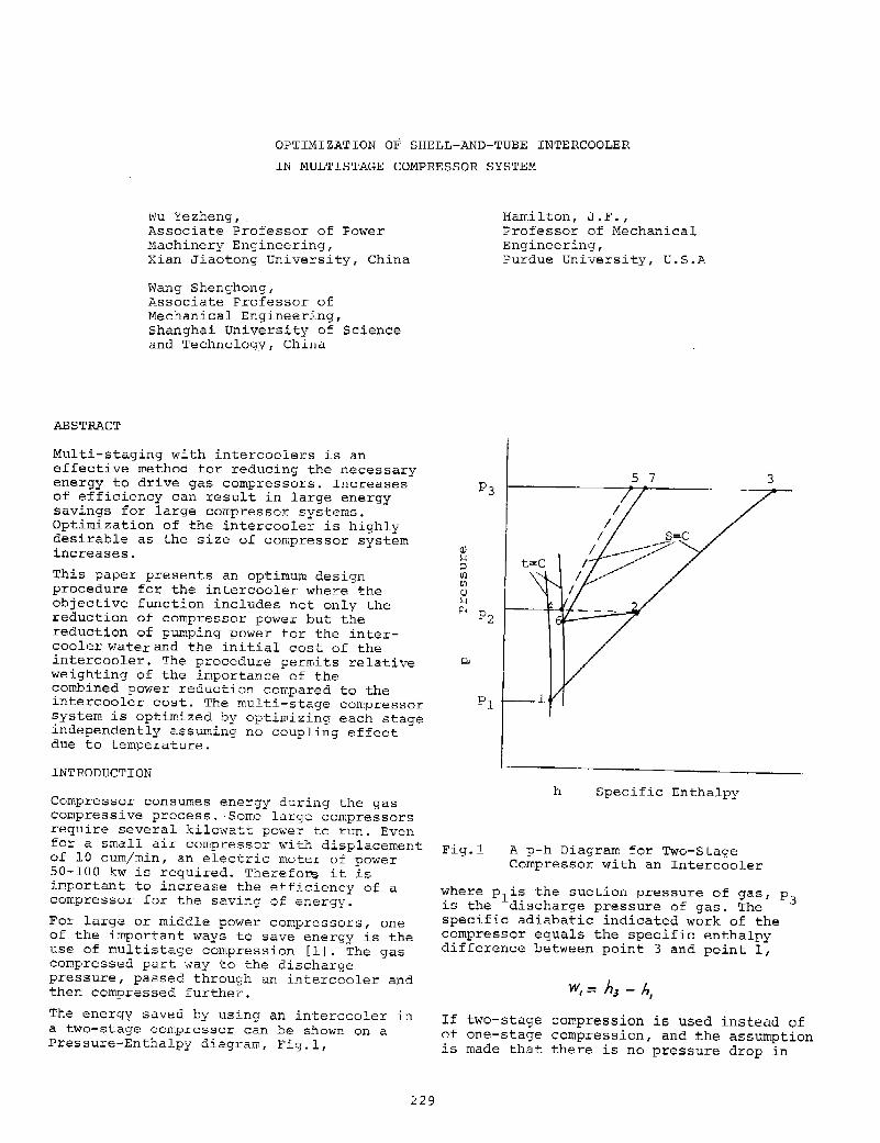
The energy saved by using an intercooler in a two-stage compressor can be shown on a Pressure-Enthalpy diagram, Fig.l,

229

Q) 1-l ::I lll tJl Q) !..; r;l.l

p2

p_,

pl

Fig.l

Hamilton, J.F., Professor of Mechanical Engineering, Purdue University, U.S.A

5 7

h Specific Enthalpy

A p-h Diagram for Two-Stage Compressor with an Intercooler

3

where p1is the suction pressure of gas, p

3 is the discharge pressure of gas. The specific adiabatic indicated work of the compressor equals the specific enthalpy difference between point 3 and point 1,

If two-stage compression is used instead of of one-stage compression, and the assumption is made that there is no pressure drop in

·the intercooler, the overall compressive process curve is 1-2-4-5. The specific adiabatic indicated work of coropressor equals

Since the slope of the process curve 4-5 is larger than the slope of the curve 1-3 and the pressure limits are equal, then

The specific work saved by using this ideal intercooler is

In fact, there is pressure drop in a nonideal intercooler, so the pressure of gas at the outlet of the intercooler is p , less than p 4 • The specific adiabatic indicgted work of compressor then equals

The actual specific work saved is

Theoretically, the higher the heat-transfer rate of the intercooler, the lower the tempe:ature t 6 will be and the greater the quantlty of energe can be saved. But it is iropossible to remove too much heat from gas to water because of the reason given below:

From a general heat-transfer rate equation

it can be seen that the heat-transfer rate Q will increase with an increase of the beat-transfer area A and the overall heat-transfer coefficient u,. But the increase of area A results in a larger size

and a higher first cost of the intercooler. Therefore, there is a cost effectiveness limitation on the heat-transfer area A. The overall heat-transfer coefficient u also has it's cost effectiveness limitation, because U depends on both the velocity of gas and the velocity of water. By forcing ~he fluids through the intercooler at higher velocity, the overall heat- transfer coefficient can be increased, but this higher velocity will result in a large pressure drop through the intercooler and correspondingly larger pumping power of fluid. There will also be a drop in the

230

specific work saved by the intercooling process.

From this discussion, it can be seen that an optimum intercooler exists and, therefor~ the purpose of this intercooler optimization is to determine the optimal heat-transfer area, the velocity of fluid, and the dimensions of the intercooler.

Generally, the intercooler is designed after the number of the compressor stages and the norminal pressures of each stage are determined. Therefore,it is assuroed in this paper that the number of stages and the nominal pressures are fixed before the intercooler optimization.

THE OBJECTIVE FUNCTION

Many papers have discussed optimum design of heat exchangers as sing-le unit.

Shah, R.K. etal [2] discussed the problem of heat-exchanger optimization for a direct-transfer crossflow intercooler where the objective function was the total fluid pumping power for the exchanger.

For a compact-in-fin heat exchanger, an objective function f was given by Mandel, S.W. etal [3].

where p is the local static pressure, Po is the tot~l pressure at inlet, and Nu is the Nusselt number. The objective function f was minimized while maintaining Reynolds number similarity.

Radhakrishnan, V.R. etal [4] made an optimum design of shell-and-tube heat exchangers using four terms in his objective function:

a. Fixed charges on the heat exchanger b. Cost of utility fluid c. Pumping cost of process fluid d. Pumping cost of utility fluid

The objective functions listed above could not be used for the optimization of compressor intercooler, .because one of the roost iroportant purposes of using intercooler in compressor system is to reduce the work of the compressor and therefore a term which directly connects with the adiabatic indicated power of compressor have to be included in the objective function. From this point of view, it is reasonable to use the following objective function for the compressor system

f= f( Cost of compressor adiabatic indicated power, .Pumping cost of cooli:~a9 water, cost of intercooler) (1)

p ,1

.. p . c,~ -,r- - ..,,---­

11 .......-+----, ,...-..+---, I I II ,,

Int. Corrp. II Int. orrp. II Int. Gas II II I II II II I L ___ 7

__ __J L _______ JL_ 7

___ .JL_----- _j Unit 1 Unit i

n Units

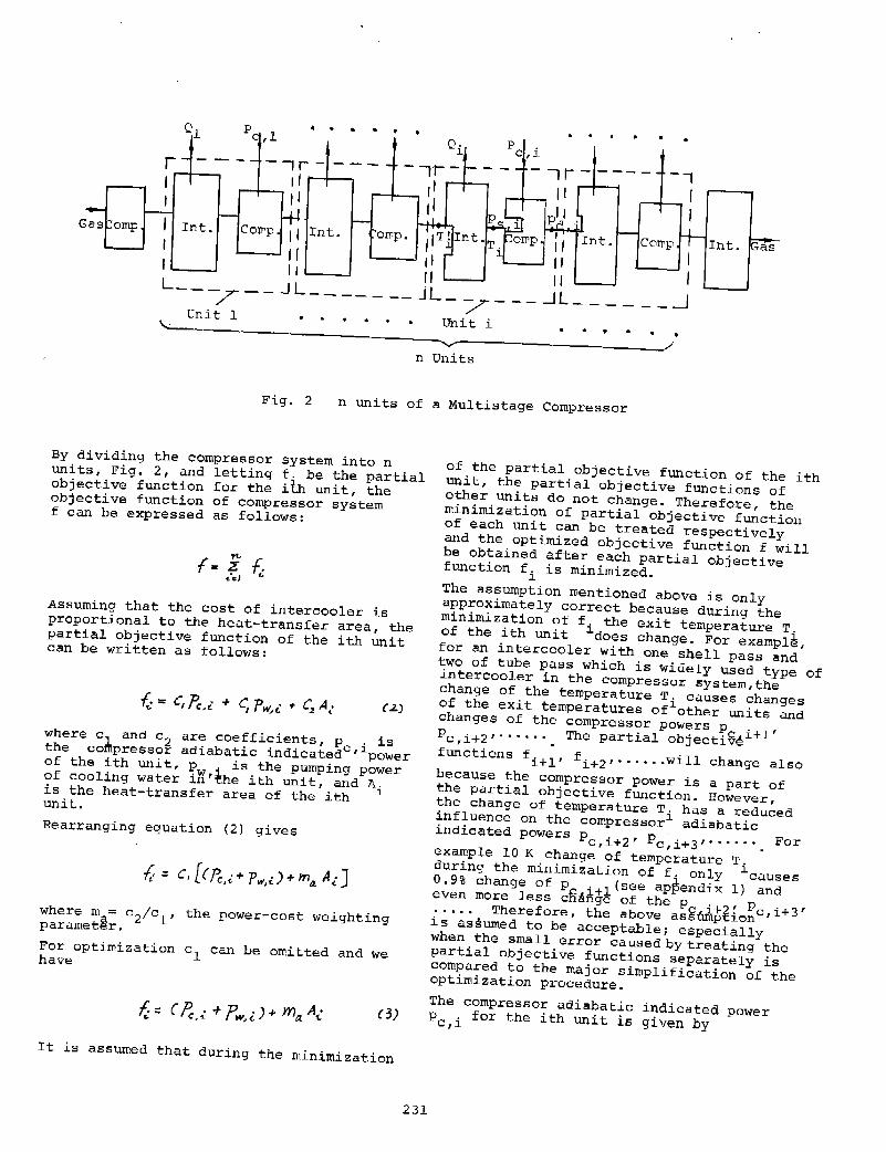
Fig. 2 n units of a Multistage Compressor

By dividing the compressor system into n units, Fig. 2, and letting f. be the partial objective function for the ith unit, the objective function of compressor system f can be expressed as follows:

Assuming that the cost of intercooler is proportional to the heat-transfer area, the partial objective function of the ith unit can be written as follows:

where c and c 2 are coefficients, p . is the co~pressor adiabatic indicatedc'~power of the ith unit, p . is the pumping power of cooling water iW'the ith unit, and A. is the heat-transfer area of the ith 1 unit. Rearranging equation (2) gives

where m ~ c2;c

1, the power-cost weighting paramet~r.

For optimization c1 can be omitted and we have

(3)

It is assumed that during the minimization

of the partial objective function of the ith unit, the partial objective functions of other units do not change. Therefore, the minimization of partial objective function of each unit can be treated respectively and the optimized objective function f will be obtained after each partial objective function f. is minimized. ~

The assumption mentioned above is only approximately correct because during the minimization of f. the exit temperature T. of the ith unit ~does change. For exampl~, for an intercooler with one shell pass and two of tube pass which is widely used type of intercooler in the compressor system,the change of the temperature T. causes changes of the exit temperatures of~other units and changes of the compressor powers p . 1

, Th · 1 b' .c..t~+ Pc,i+2 ,....... e part~a o ]ect~v~ functions fi+l' fi+2 , •.••.• will change also because the compressor power is a part of the partial objective function. However, the change of temperature T. has a reduced influence on the corepressor~ adiabatic indicated powers p .+2 ' p · .+3 , •..•.• For c,~ c,~ . example 10 K change of temperature T. during the minimization of f. only ~causes 0.9% change of p i+l(see ap~endix 1) and even more less cHAnge of the p '+2 ' p .+3 ' •.•.• Therefore, the above as~uffiptionc,~ is assumed to be acceptable; especially when the small error caused by treating the partial objective functions separately is compared to the major simplification of the optimization procedure.

The compressor adiabatic indicated power p . for the ith unit is given by c,1

231

(I})

The pressure drops LIP and ~pd of gas passing through the scompressor valves are

assumed to be fixed, so they have no influence on the intercooler optimization

and do not appear in equation (4).

To determine the exit temperature T., the

following equations have been used: 1

a. Equation for heat flow rate Q

Q 2: ( h,.n - h~tJ.t) • M

Q is also the heat-transfer rate.

b. Equation for overall heat-transfer coefficient U

c. Equation for heat-transfer coefficient

o<.m in gas side

d. Equation for heat-transfer coefficient

o< in water side w

To determine the pressure drop AP., the following equation has been used: 1

AN EXAMPLE

An intercooler listed in literature [5] has

been used as an example. This is an inter­

cooler with mass flow of gas of 6480 kg/hr.

The inter~oo12r recdves gas at a pressure of 175Kl0 N/m and cools it to a temperature

of 325K. The cooled gas can then be 4 2 compressed in a cowpressor up to 525xl0 N/m,

The parameters of the intercooler before the

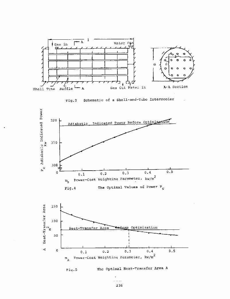
optimization are (see Fig. 3)

d 0- The diameter of tube, d 0

= 0.025 m

232

n 2- Number of columus of tube, n 2= 21

n 3- Number of rows of tube, n 3= 18

1 - Length of tube, 1= 2.28m

Ni- Number of baffles, Ni= 13

V - The velocity of the cooling water, w V = 0.16m/sec

w The optimization problem of this intercooler

can be restated in the following form:

Minimize: { = f ( V. I n n I .J ) w> Clo' J., J, t.., IVi

Subject to the inequality constraints

l- o.:J.S'J> N· ;;: o.o6

t

and the variable boundary constraints

o.ttf....:: Vw < o • .:z.o

~o..::::. n.z...::::: 35

t5" < n" < 2S

2 < L < 4

JO <IV._ <3D

The values of the contraints are given arbitrary in accord with the author's experience.

The optimization problem is solved by using the Generalized Reduced Gradient Method which is one of the w.ost efficient

optimization method and has been coded as OPT in Purdue University [6] [7].

The optimization is made under different

values of power-cost weighting parameter

m~ so that we can evaluate the effect c~used by different casts of the inter­cooler.

When coefficient m = 0, equation (3) reduces to a

f= fc + Pw

where only the thermodynamic performance

is chosen as the objective function. The

total power consumed before and after the

optimization are 323.5kw and 310.0 kw

respectively, i.e., 13.5 kw has been saved after the optimization.

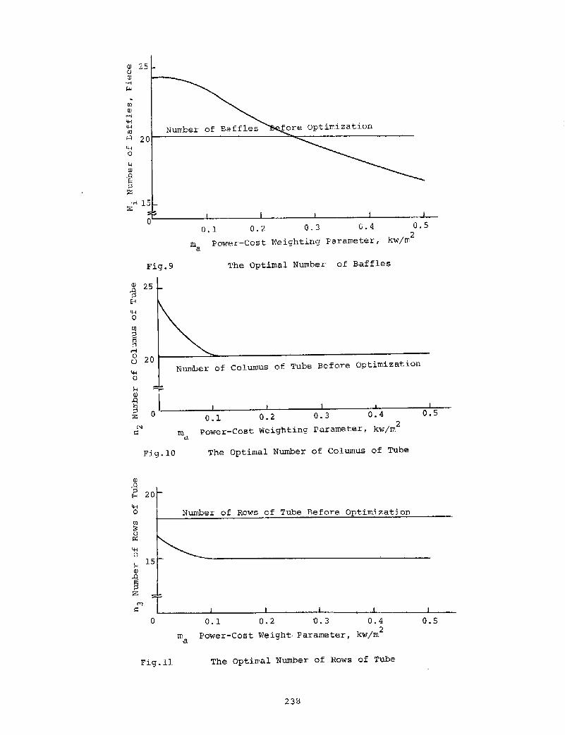
Figures 4 through 6 show the optimal values of the compressor adiabatic indicated power p , the heat- transfer area A and the v~locity of water v plotted against the weighting coefficie~t m . a From Fig. 4&5, it can be seen that the power p increases with the increase of the coefficient m , while the heat-transfer area A reduces awith the increase of coefficient m • The shape of the curves can be explained gs follows: With the increase of coefficient m , the cost of the intercooler plays a mo~e and more important role in the objective function. Therefore, the heat-transfer area has to be reduced with the increase of coefficient rn even though it will cause the increase 8f the power. The optimal area A is equal to the original value given before the optimization when m '=0.31,· and A must be lower than the origi~al value when ma>0.31. The minimuro objective function can be obtained by the increase of the area A only when ma~0.31. From Fig. 7&8, it can be seen that the optimal length and the optimal diameter of the tube are reduced with an increase of the coefficient m , because the heat-transfer area reduces. a In Fig. 9, the nurober of baffles N. is reduced when the coefficient m islincreaced because the length of the tubeaalso decreaced and there is a constraints to keep the

Water

distance between two baffles from becoming too small.

Fig. 10&11 show the changes of n, and n 3 with the coefficient m • Since tfie change are quite small , the avalues of n2 and n

3 can be taken as constants after rna~ 0.1.

CONCLUSION

Additional terms as well as the compressor adiabatic indicated power should be included in the objective function used for the intercooler optiroization in a compressor system. Therefore, an objective function f including the cost of the compressor adiabatic indicated power, the pumping cost of cooling water and the cost of intercooler has been presented. The objective function of the compressor system f can be obtained by dividing the compressor system into multiple units and then minimizing the partial objective functions of each unit.

APPENDIX

For the (i+l)th unit (see Fig.l2), the heat flow rate Qi+l equals

(t?.)

Water

tout,i t. tout,i+l t. . 1 ln ln,l+

r -l I I I I I

Gas IT!

- -- -- -- I r- -- - ------1 Ps,i

T. l

Int.

...____,

Fig. 12

I I Ps,i+l I

I I I I I Ti+l

I I I

Camp. l I Int. Camp I I I I ..........__.

I Gas Tl+l p p I d,l+l 1

d, l I _ __( L ___ \ _ _j

(i+l) th Unit

The Schematic of unit i and unit(i+l)

233

On the other hand, 6. 1 can be determined

by heat-transfer rat~+ equation

where

Since

A!J ;: r._.;, - f.:'i"t

A fw = fou'(, t'.,f - t;,., t'+l

~ = ~~' - tr-ut,i+l

B~ = Tt"+l - t:,, -r:~r

~ "& >> Afw, J&J 7j.z- At.:"' .4 ~ and

Letting( t t '+l+ t. . 1 )~ t. 1

and ou ,~ ~n,~+ ~+

ci:J)

([)

comparing equation(c) with equation(a),

have we

Therefore

.2 ~·:, - t,'t-1 2 ~·~,- (..,.,

::= c (t!)

Where C D·A C . TJ M·c . ~s a constant because

pro

of the (i+l)th unit nearly have no change

during the optimization of the ith unit.

Rearranging equation(e) and derivating the

both sides, we have

I

d (.21i+t- ti+t)

.27'...:, - t .. ·-t I c{;

..2 1.,;.,, - t<.'tl

and then

Since the temperature change of water is

quite small than the temperature change of

gas, clt;~t << 2 , we have

dr~,,

d T,;.,, :=. _2_!-'-:i+i--/_-_t_,·t_l_ + .!. J f ... .,., JT,;, 2-1(;,- t.,:+l 2. d~~l

Ci)

According to the engineering practice, the

temperatures usually can be approximately

taken as

-r/ ,/ t dt,..,., ;;_._,, ~J~JK rt'.,== .,.~J J.<. ,:,.,::till< d~=~.f

/ ,I ) 1.'+1

Therefore,

cJ 4't I J r,;, = D./f

For isentropic process, we have

k-1 , T

"..,., ::= i,: E.

where £ is the ratio of pressure in the ith

unit, and k is the ratio of specific heats.

usually, f.='· For the mixture of H

2 and N2

, k: 1.4, hance

It means that the lOK change of temperature

T i wi 11 cause 2. 6 K change of temperature

Ti+l"

From equation(4)

pd . 1 and p '+l are norminal pressure of ,~+ S,l-

the (i+l)th stage. They are fixed before

the optimization. p.+l is the pressure drop

of the (i+l)th unit: Since the intercooler

size of the (i+l)th unit has no change

during the optimization of the ith unit, the

velocity change of gas in the (i+l)th unit

caused by the change of the teroperature T.

is also very small. Therefore, the change~

of the pressure drop pi+l is negletable,

and we have

234

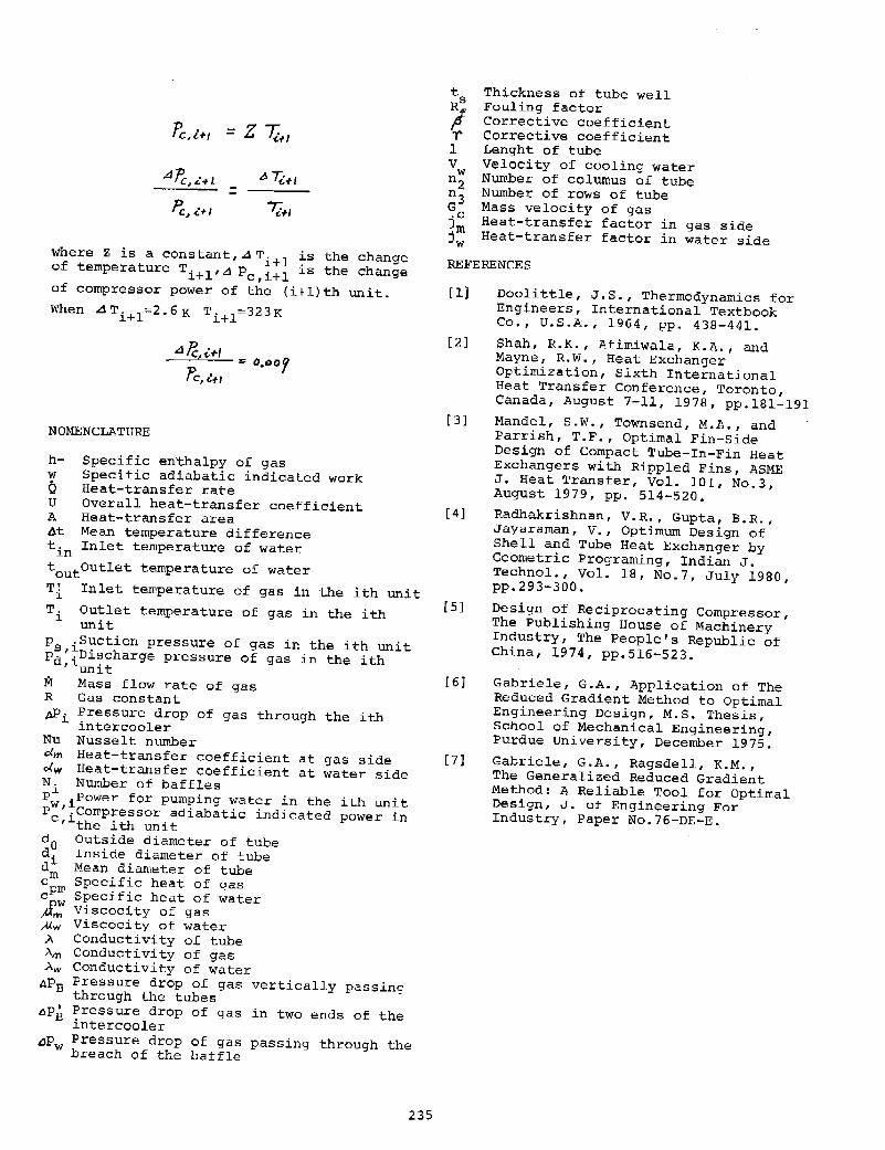
Pc,ll-t = z 7if1

Af, . I C, <.+" ~ Ti+t =

Pc .. ~.+t 7i#-t

where Z is a constant, ..:\ T. + 1 is the change of temperature Ti+l'.d Pc,~+l is the change of compressor power of the (i+l)th unit. When ..dTi+l""2.6K Ti+l=323K

NOMENCLATURE

Ll Pc,il-1

f'c,.:~-t

h- Specific enthalpy of gas w Specific adiabatic indicated work Q Heat-transfer rate U Overall heat-transfer coefficient A Heat-transfer area ~t Mean temperature difference t. Inlet temperature of water 1n toutoutlet temperature of water Ti Inlet te~perature of gas in the ith unit T. Outlet temperature of gas in the ith 1

unit ps .Suction pressure of gas in the ith unit Pa'7Discharge pressure of gas in the ith

'1unit

M Mass flow rate of gas R Gas constant APi Pressure drop of gas through the ith

intercooler Nu Nusselt n~ber dm Heat-transfer coefficient at gas side ~w Heat-transfer coefficient at water side N. Number of baffles P 1 .Power for pumping water in the ith unit Pw'7cowpressor adiabatic indicated power in c,J.the ith unit d

0 Outside diameter of tube d. Inside diameter of tube d 1 Mean diameter of tube em Specific heat of gas cpro Specific heat of water ~: Viscocity of gas .AJ.w Viscocity of water A Conductivity of tube .\,11 Conductivity of gas Aw Conductivity of water

APB Pressure drop of gas vertically passinq through the tubes ~PE Pressure drop of gas in two ends of the

intercooler .dPw Pressure drop of gas passing through the

breach of the baffle

t Thickness of tube well Rs Fouling factor I Corrective coefficient r Corrective coefficient 1 Lenght of tube v Velocity of cooling water w Number of columus of tube n2

Number of rows of tube n3 G Mass velocity of gas .c Heat-transfer factor in side ~m gas Jw Heat-transfer factor in water side

REFERENCES

[1] Doolittle, J.S., Thermodynamics for Engineers, International Textbook Co., U.S.A., 1964, pp. 438-441.

[2]

[3]

[4]

[5]

[6]

[7]

Shah, R.K., Afi~iwala, K.A., and Mayne, R.w., Heat Exchanger Optimization, Sixth International Heat Transfer Conference, Toronto, Canada, August 7-11, 1978, pp.l81-191 Mandel, S.W., Townsend, M.A., and Parrish, T.F., Optimal Fin-Side Design of Compact Tube-In-Fin Heat Exchangers with Rippled Fins, ASME J. Heat Transfer, Vol. 101, No.3, August 1979, pp. 514-520. Radhakrishnan, V.R., Gupta, B.R., Jayaraman, V., Optimum Design of Shell and Tube Heat Exchanger by Geometric Programing, Indian J. Technol., Vol. 18, No.7, July 1980, pp.293-300.

Design of Reciprocating Compressor, The Publishing House of Machinery Industry, The People's Republic of China, 1974, pp.516-523.

Gabriele, G.A., Application of The Reduced Gradient Method to Optimal Engineering Design, M.S. Thesis, School of Mechanical Engineering, Purdue University, December 1975. Gabriele, G.A., Ragsdell, K.M., The Generalized Reduced Gradient Method: A Reliable Tool for Optimal Design, J. of Engineering For Industry, Paper No.76-DE-E.

235

Shell Tube

(1j (j) 1-1

,.,;:

1-1 (j)

320

310

150

':ri 100 ~ <tlN

l-1 = E-<

L so (1j (j) ~

0

Gas in A-A Section

Fig.3 Schematic of a Shell-and-Tube Intercooler

Adiabatic

0.1 0.2 0.3 0.4

m a Power-Cost Weighting Parameter, kw/m

2

Fig.4 The Optimal Values of Power Pc

Heat-Transfer Area

0.1 0.2 0.3 0.4

rna Power-Cost Weighting Parameter, kw/m2

0.5

0.5

Fig.S The Optimal Heat-Transfer Area A

236

0.20

H 0.18 Q)

+' Ill :;:: Velocity of Y.Tater Before Optirrization

4-1 0.16

0 u

>.QJ +'Ill 0.14 ·.-f .......... u e 0

..-1

~ 0.12

:;:." 1 0

0.1 0.4 0.5 0.2 0.3 ma Power-Cost Weighting Paraweter, kw/m2

Fig.6 The Optimal Velocity of Water

4.0

Q) .a ::I 8

11--i 0 3.0

.s:: +' E'i ~ ~ Q)

...:I

..-1 2.0

m a

Fig.7

0.030

Length of Tube Before Optimization

0.2 0.3 Power-Cost Weighting Parameter,

0.4

kw/m2

The Optimal Length of Tube

0.5

0.025 Outside Diarreter

0.020

0

Fig.B

0.2 0.3 ".4. rower-Cost Weiqhting FaraiTeter

0.5 2

kw/rr. The Optimal Outside Diamet~r of Tube

237

I]) 25 u I])

·.-i >'-<

til I])

.-J 4-1 'H aj I'Ll 20 'H 0

f-1 I])

.Q !': :;l z

·.-\ 15 :z

0

Fig.9

I]) 25 .g 8

'H 0

[jJ ;:I

§ .-J

m a

O.l 0.2 0.3 0.4

Power-Cost v1eighting Parameter,

0.5 2

kw/m

The Optimal Number of Baffles

3 20 ~------~~------------~------------------------Number of Colurnus of Tube Before Optimization

1!-1 0

1-1 .-,...

i oi'--------~--------L-------~--------~--------L---0.1 0.2 0.3 0.4 o.s ma Power-Cost Weighting Parameter, kw/rn

2

Fig.lO The Optimal Number of Columus of Tube

I]) .Q ;:I 8

'H 0 Number of Rows of Tube Before Optimization til ;.'!: a 'H 0

1-1 (!)

~ :;l :z

<'") 1 !=:

0 0.1 0.2 0.3 0.4 o.s rna Power-Cost Weight Parameter, kwjm

2

Fig .11 The Opti~al Number of Rows of Tube

238