Accepted Manuscript

Title: Deep-bed filtration model with multistage depositionkinetics

Authors: Vitaly Gitis, Isaak Rubinstein, Maya Livshits,Gennady Ziskind

PII: S1385-8947(10)00644-3DOI: doi:10.1016/j.cej.2010.07.044Reference: CEJ 7155

To appear in: Chemical Engineering Journal

Received date: 1-6-2010Revised date: 11-7-2010Accepted date: 19-7-2010

Please cite this article as: V. Gitis, I. Rubinstein, M. Livshits, G. Ziskind, Deep-bedfiltration model with multistage deposition kinetics, Chemical Engineering Journal(2010), doi:10.1016/j.cej.2010.07.044

This is a PDF file of an unedited manuscript that has been accepted for publication.As a service to our customers we are providing this early version of the manuscript.The manuscript will undergo copyediting, typesetting, and review of the resulting proofbefore it is published in its final form. Please note that during the production processerrors may be discovered which could affect the content, and all legal disclaimers thatapply to the journal pertain.

Page 1 of 33

Accep

ted

Man

uscr

ipt

Deep-bed filtration model with multistage deposition kinetics

Vitaly Gitis a,*, Isaak Rubinstein

b, Maya Livshits

c, Gennady Ziskind

c

a,

* Corresponding author: Unit of Environmental Engineering, Ben-Gurion University of the Negev,

P.O. Box 653, Beer-Sheva 84105, Israel, e-mail gitis@bgu.ac.il

b Blaustein Institutes for Desert Research, Ben-Gurion University of the Negev, Sede Boqer Campus

84990, Israel

c Department of Mechanical Engineering, Ben-Gurion University of the Negev, P.O.Box 653,

Beer-Sheva 84105, Israel

*Revised Manuscript

Page 2 of 33

Accep

ted

Man

uscr

ipt

Gitis et al. Page 1 of 33

Abstract

In the present study, a phenomenological model of deep-bed filtration is suggested. It combines an

advection-dispersion equation with an equation of nonlinear multistage accumulation kinetics. The

model includes dispersion and accounts for temporal and spatial changes in media porosity.

It is suggested that at any location inside the column the filter deposit is formed first as an

irreversible ripening layer, followed by formation of reversible deposit during the operable stage. The

latter continues until the deposit reaches locally its maximum value. Then, filter breakthrough takes

place.

The equations are solved numerically, using an explicit finite-difference scheme. The results

compare favorably with laboratory experiments at an EPA facility, and with field experiments

performed by Mekorot – Israeli Water Company.

Keywords – Deep-Bed Filtration; Porous Media; Mathematical Modeling; Accumulation Kinetics;

Particle; Packed Bed

Page 3 of 33

Accep

ted

Man

uscr

ipt

Gitis et al. Page 2 of 33

Nomenclature

aL coefficient of longitudinal dispersivity, m

C mass concentration of particles in suspension, kg/m3

dc average diameter of filter grain, m

dp average particle diameter, m

D effective dispersion coefficient, m2/h

J particle flux, kg/m2 h

Ka attachment rate coefficient in the operable stage, 1/m

Kd detachment rate coefficient in the operable stage, 1/h

Kr attachment rate coefficient in the ripening stage, 1/m

L filter depth, m

t time, h

u longitudinal approach velocity, m/h

z position in the column measured as a distance in longitudinal direction (direction of flow), m

Greek letters

diffusion number in numerical scheme

γ Courant number in numerical scheme

ε local bed porosity at time t

λ filter coefficient, 1/m

μ absolute viscosity of suspension, kg/m h

ρ density of particle material, kg/m3

σ specific deposit, kg/m3

σr transient specific deposit, kg/m3

σu ultimate specific deposit, kg/m3

Operators

B~

dimensionless form of variable B

Subscripts

0 initial value

Page 4 of 33

Accep

ted

Man

uscr

ipt

Gitis et al. Page 3 of 33

1. Introduction

Rapid granular filtration is one of the widely implemented treatment methods for relatively dilute

aqueous suspensions. In this method, the grains of a porous medium, like sand, anthracite, tuff, etc.,

adsorb up to 85% by mass of suspended particles [1], transported by water inside the filter bed. To

ensure a high quality of the tap water, it is essential to understand filtration kinetics and to predict

filter performance through physically-sound modeling.

The beginning of deep-bed filtration theory dates back to more than a half-century ago and is

associated with the works of Iwasaki [2] and Minz [3]. Filtration models are commonly classified as

phenomenological, stochastic or trajectory ones [4]. In spite of the fact that the latter are better

justified, their practical application is limited to simple geometric representations that reflect clean

bed conditions only. Experimental validation of the trajectory models often has limited success, thus

requiring introduction of numerous empirical coefficients, typical of stochastic and

phenomenological models, whereas the latter ones often incorporate implicitly some information

about the stochastic aspects of mass transfer.

The deep bed filtration can basically be viewed on a macroscopic or microscopic level. The

microscopic view is usually presented as a sequence of transport and attachment steps where the

transport is discussed in view of five transport mechanisms, namely interception, inertia, diffusion,

sedimentation and local turbulence [5] and the attachment is viewed through the van der Waals

attraction and electrostatic repulsion of two entities, a particle and a media grain. This allows

obtaining a “filter coefficient” which is then introduced into a macroscopic model. State-of-the art of

the macroscopic filtration modeling of hydrosols and aerosols is presented in a recent book by Tien

and Ramarao [6]. Apparently, such models are widely used also in petroleum engineering. For

instance, Guedes et al. [7] analyze deep bed filtration under multiple particle-capture mechanisms and

conclude that it is possible to reflect them in a single coefficient. A review paper by Zamani and

Maini [8] analyzes microscopic and macroscopic models, discussing advantages of the latter in

prediction of the removal efficiency of deep bed filtration process. It is stated that predicting the filter

Page 5 of 33

Accep

ted

Man

uscr

ipt

Gitis et al. Page 4 of 33

performance by a macroscopic model requires the knowledge of filter coefficient, which can be

obtained by using a search optimization technique along with effluent concentration history. Alvarez

et al. [9] argue that the filtration function, which is the fraction of particles captured per unit particle

path length, cannot be measured directly and thus must be calculated indirectly by solving inverse

problems. As the practical petroleum and environmental engineering situations require knowledge of

particle penetration depth, they determine this quantity from effluent concentration histories

measured in one-dimensional laboratory experiments.

Macroscopically, filtration process may be described as a change in concentration, C, of the

suspended particles with time, t, whereas a local mass conservation law is combined with an

accumulation kinetics' equation. The kinetic equation for particle capturing process is generally

expressed as

,CFt

, where is the specific deposit, defined as the amount of material

deposited per unit volume of the filter. An analysis of the existing literature shows [6, 10] that there

exist two alternative approaches to F(C,), which reflect the accumulation kinetics:

1. Irreversible accumulation, meaning that a suspended particle, once retained by the porous bed,

is never entrained by the flow again [2, 11-14]. The respective equations of attachment kinetics

of this type have the general form of Cut

, with various models differing in the way of

specifying the filter coefficient, . Generally, is not constant throughout the filtration

process.

2. Reversible accumulation, meaning that a suspended particle is alternately deposited and ripped

off by the flow [3, 15]. The respective equation of accumulation kinetics is

da KuCKt

, with the phenomenological attachment and detachment coefficients, Ka

and Kd, specified empirically.

The main difference between the two approaches lies in their treatment of an experimentally

evidenced breakthrough stage of filtration, where the presence of suspended particles increases [16].

Page 6 of 33

Accep

ted

Man

uscr

ipt

Gitis et al. Page 5 of 33

According to the first approach, the breakthrough occurs when the media pores become so narrow

that under constant feed the interstitial velocity does not allow the suspended particles to adhere

[11, 17]. The second approach implies that tearing of discrete (original) particles off the deposit by

shear forces is as obvious as in flocculation [18].

The models reported in the literature have greatly enhanced our understanding of the mechanisms

behind deep-bed filtration and provided useful insights in specific practical applications. An analysis

of the literature shows, however, that the existing models are mutually excluding: they imply that the

filtration cycle contains either the ripening and operation stages, as in an irreversible deposition mode,

or operation and breakthrough stages, as in a reversible deposition mode. Thus, each of these two

approaches disregards one of the stages of the filtration process evidenced from the experiments [16].

Being aware of this problem, the followers of the irreversible approach introduced complex filtration

coefficients [5] that at a certain level of the specific deposit caused decrease in filtration efficiency, in

order to account for the breakthrough stage. On the other hand, in the reversible deposition models a

dashed line is commonly hand-added to the predicted filtration curves in order to reflect the excluded

ripening stage [15]. Thus, in any of the approaches the full filtration cycle was not predicted or at least

reflected. As a result, an accurate representation of the entire cycle was difficult if not impossible

[19].

The model suggested herein fuses the kinetic approaches previously viewed as mutually excluding.

It comprises two differential equations: a full mass balance equation and a multistage-kinetics

equation. Specifically, at any given depth inside the filter, the model differentiates between the

following three stages in the accumulation of suspended particles:

1. Ripening stage – irreversible formation of deposit monolayer on filter medium.

2. Operable stage – consequent reversible deposit growth.

3. Breakthrough stage – halt of further accumulation upon reaching, locally, a certain amount of the

deposited material.

Page 7 of 33

Accep

ted

Man

uscr

ipt

Gitis et al. Page 6 of 33

A closed system of coupled partial and ordinary differential equations, with appropriate boundary

and initial conditions, is solved numerically by the method of finite differences. The results of the full

numerical solution are analyzed and compared with the performance of a laboratory-scale filtration

plant which was designed and constructed specifically for this task. In addition, the model predictions

are compared with the data of field experiments performed by the Mekorot Water Company in Israel.

2. Model

The model suggested herein is based on the following physical picture. An aqueous dilute

colloidal suspension is fed through a filter bed which initially contains no deposit. At the beginning,

passing colloids may settle as separate particles covering filter grains with a monolayer deposit [14].

This is the ripening stage recognized in filtration concentration plots by relatively low retention. The

ripening lasts until the upstream surface of media grains becomes coated with single particles, or until

the occasional dendrites formed on the grains evolve into a monolayer through proliferation onto the

uncovered part of the grain surface [13, 20]. Once the born particles start to interact primarily with the

previously deposited ones, the retention efficiency increases and the filtration cycle is entering the

operable stage. Here, both attachment of the suspended particles and their re-entrainment by the flow

occur in parallel [21]. The transition from the irreversible to reversible deposition mode takes place

when the specific deposit attains a prescribed transitional value, σr.

Since the volume of particles that can be hold by the filter is finite, eventually a saturation stage is

achieved when the bed local specific deposit reaches its maximum feasible value, σu. From this

moment on, it is assumed that further accumulation effectively stops at that location, and thus any

suspended particles are only transferred along the transport channels formed in the bed [22-23].

The approach adopted in the present study is based on the assumption that particle concentration in

the stream, C, is uniform across the filter cross-section. Also, the approach velocity, u, is assumed to

be uniform. Accordingly, the expected specific deposit, , is uniform across the cross-section, too.

Page 8 of 33

Accep

ted

Man

uscr

ipt

Gitis et al. Page 7 of 33

These common assumptions mean that the present model is one-dimensional in space, i.e. both the

concentration and specific deposit depend on the z-coordinate, which denotes the filter depth, and

also on time.

Each filter bed slice between the cross-sections at z and z+z is characterized by mass balance

comprised by the following four factors: incoming particle flux jz, outcoming particle flux jz+z, rate

of particle deposition/re-entrainment ∂/∂t, and the resulting rate of change of particle concentration

in the feed, ∂C/∂t. Accordingly, the species conservation equation attains the following form:

jztt

C

(1)

It is important to note that the first term on the left-hand side of Eq. (1) includes also the local porosity,

, and this in order to take into account the changes in the fluid volume due to the increasing deposit.

It is obvious that is time-dependent at any location inside the bed.

The particle flux, j, includes both dispersion and convection contributions:

zCDuCj

(2)

where D is the effective dispersion coefficient.

The outlined above three different stages of filtration are described by the following kinetic

equation for the accumulation rate, ∂/∂t:

0

da

rdef

KuCK

uCK

t when

u

ur

r

0

(3)

where Kr is the attachment rate coefficient at the ripening stage; Ka is the attachment rate coefficient

at the operable stage; Kd is the detachment rate coefficient at the operable stage; r is a threshold

specific deposit value, corresponding to the transition from the ripening to the operable stage; and u

is the ultimate specific deposit value, which indicates the filter retention capacity limit. It is important

Page 9 of 33

Accep

ted

Man

uscr

ipt

Gitis et al. Page 8 of 33

to emphasize that the values of are compared to the preset limits, r and u, locally, reflecting the

real situation in which various stages coexist inside the filter bed at the same instant, depending on the

cross-section location. It is worth to note also that the expression of Eq. (3) defines the general case of

multistage transition and might be reduced to particular cases of irreversible and reversible

attachment [15, 24].

The local porosity, , is related to its initial value 0 and the specific deposit through the relation

0

(4)

where is the physical deposit layer density, assumed constant for simplicity.

Equations (1-4) form a closed system of coupled partial and ordinary differential equations for

tzC , and tz,’ which requires a set of appropriate boundary and initial conditions. Reflecting a

constant or near constant concentration of impurities in the feed water taken from a large reservoir, a

specific, constant concentration of particles in the feed suspension is assumed at the entrance to the

column:

0,00 tzatCC (5)

The Danckwerts exit criterion [25], which assumes that there is no concentration change at the exit

from the filter bed, is adopted as the second boundary condition:

0,0

tLzat

z

C

(6)

The initial conditions correspond to a clean bed before the filtration starts:

0)0,( zC (7)

00, z (8)

The complete model presented above requires a numerical solution, which will be discussed in the

Page 10 of 33

Accep

ted

Man

uscr

ipt

Gitis et al. Page 9 of 33

next section. We note that upon setting D=0, ε=const, σr→, the system of Eqs. (1-4) is reduced to

the much simpler case of a linear attachment-advection model. The latter yields a classical Cauchy

problem for a first-order linear hyperbolic equation, and may be solved in a straightforward manner

by the method of characteristics [26]. However, such solution would be practically limited to the first

filtration stage.

3. Numerical solution

The initial/boundary value problem, defined by Eqs. (1-8), is solved numerically by the method of

finite differences. For this purpose, the equations are rendered dimensionless, using the following

definitions:

00

~~

~~

C

CC

C

L

utt

L

zz

(9)

where L is the filter length, u is the approach velocity, and C0 is the concentration at the entrance to

the filter.

An explicit algorithm is used for the numerical solution. From the stability considerations, a

backward-forward finite difference scheme has been chosen, with the first-order backward advective

derivative and forward time derivative. The dispersion term was approximated using a second-order

central difference scheme. The specific deposit was calculated by a fourth-order Runge-Kutta

scheme [27]. The filter length was subdivided into 100 equal grid steps.

To ensure stability of the implemented scheme, the time step is limited by the criteria based on the

Courant number, γ, and diffusion number, , respectively defined as:

z

t~

~

Page 11 of 33

Accep

ted

Man

uscr

ipt

Gitis et al. Page 10 of 33

2~

~1

z

t

Pe

(10)

where t and z are the dimensionless time and space steps, respectively, and the “numerical”

mass Peclet number is defined as Pe=uz/D, according to [28, 29]. It has been found empirically that

in order to ensure stability, the values of γ and must be smaller than 0.4, which is slightly more

conservative than γ<1 and <0.5 found in the literature [29].

Data input for each numerical simulation includes the filter depth, approach velocity and

approximate run time. The computer code is written in Visual C++.

As shown in the previous section, formulation of the problem requires determination of a number

of quantities, including the hydrodynamic dispersion coefficient, D, attachment rate coefficients in

the ripening and operable stages, Kr and Ka, respectively, detachment rate coefficient in the operable

stage, Kd, threshold specific deposit, σr, and ultimate specific deposit, σu. The values of these

parameters are assigned based on the literature, even though their accuracy may be questionable [5].

The values found in the literature are summarized in Table 1. One can see that each parameter is

represented by a range rather than by a specific value.

The hydrodynamic dispersion coefficient, D , can be estimated as

uaD L~ (11)

where aL is the coefficient of longitudinal dispersivity. It was found experimentally that it is of the

order of magnitude of the average sand grain size [30]. For instance, for the grain diameter of 1 mm,

we have aL~10-3

m, which for the typical approach velocities of several dozens of meters per hour

yields D~10-6

-10-5

m2/s.

In the suggested model, ripening is a fast irreversible process characterized by interactions

between particles and media grains. Accordingly, the attachment rate coefficient, Kr, may be assumed

constant throughout this stage. This is different from the previous models [11, 13, 31], where the

particle-particle collisions are assumed to determine the entire run, thus prescribing changes in the

Page 12 of 33

Accep

ted

Man

uscr

ipt

Gitis et al. Page 11 of 33

filtration coefficient even during the ripening stage. The assumption of constant Kr allows its

computation based on the initial filter coefficient for a clean bed, 0. For this purpose, the trajectory

models of Choo and Tien [32] and Rajagopalan and Tien [33] were used. For the conditions defined

in the caption of Fig. 1, the values of Kr = 3.1 m-1

and Kr = 1.5 m-1

were obtained. Based on these

results and on a comparison with experimental data, the values in a range of 0.8 to 2.5 m-1

were used

for Kr in our calculations, as presented in Table 1.

The attachment rate coefficient at the reversible growth stage, Ka, is higher than Kr. This result,

evident from a general form of the concentration plot and generally agreed among the researchers, is

caused by a transition from particle-bed interactions at the ripening stage to particle-particle

interactions at the operable stage. Whereas the previous models were based on a continuous

improvement of the filter coefficient as a function of the specific deposit, we assume that there is no

significant change in the attachment rate coefficient within a certain stage. Therefore, the attachment

rate coefficient at the reversible growth stage, Ka, is considered constant. Table 1 summarizes its

values reported in the literature. One can see that considerable deviations exist between the results

reported by different researchers.

Although some expressions for the detachment rate coefficient, Kd , are suggested in the literature

[34], its experimentally found values fluctuate significantly between various filtration sites as a result

of the differences in suspension composition, filter material, filtration regime, and a variety of other

factors. In the current study, the values of Kd were estimated by averaging its values reported in the

literature for the models with reversible deposition kinetics [3, 15], see Table 1.

It is quite difficult to evaluate the specific deposit threshold value, r, in the absence of direct

experimental data. Based on physical considerations, its order of magnitude can be estimated for

given conditions assuming that it corresponds to the most dense particle monolayer on the upper half

of grain surface. For instance, for the grain diameter of 1 mm and particle diameter of 1 m, the value

of r would not exceed 0.5 mg/cm3, i.e. the order of unity when expressed in milligrams per cubic

centimeter.

Page 13 of 33

Accep

ted

Man

uscr

ipt

Gitis et al. Page 12 of 33

Whereas the operable stage is characterized by an increase in the effective hydraulic diameter of

the grain due to the attached deposit, the subsequent breakthrough stage involves formation of

transport channels inside the filter bed. This transition occurs locally when the specific deposit

reaches the threshold value, u, which depends on media grain, filtration velocity,

coagulation/flocculation regime and several other factors. The only model that considered the

deposition mode transition was suggested by Tien et al. [14], who indicated that the pores were

blocked at 50 mg/cm3. It was suggested to determine the value ofu based on the best fit method. The

experimentally found values were in the range of 9.5 to 20 mg/cm3.

4. Test runs of the model

The presented above model was run to obtain the results shown in Figs. 1-5. A hypothetical

one-meter-deep column, fed with a dilute solution at the approach velocity of 10 m/h, was simulated

using the parameters listed in Table 1. Simulations included effects on particle removal and specific

deposit accumulation of such parameters as the run time, suspended particles’ concentration, bed

depth, deposit layer density, initial bed porosity, attachment rate coefficients in the ripening and

operable stages, Kr and Ka, respectively, detachment rate coefficient in the operable stage, Kd,

transient specific deposit, σr, and ultimate specific deposit, σu. Some essential findings are presented

in Figs. 1-5. It is worth to note that the curves in these figures reflect the well-known filter operation

curve observed in experiments and reported in the literature. Recall that the full curve generally has

three stages: ripening, efficient filtration and breakthrough [16]. The calculated curves, presented in

Figs. 1-5, are intentionally focused on specific stages of filtration, and thus not necessarily represent

the entire cycle. This is done in order to allow a discussion of subtle details.

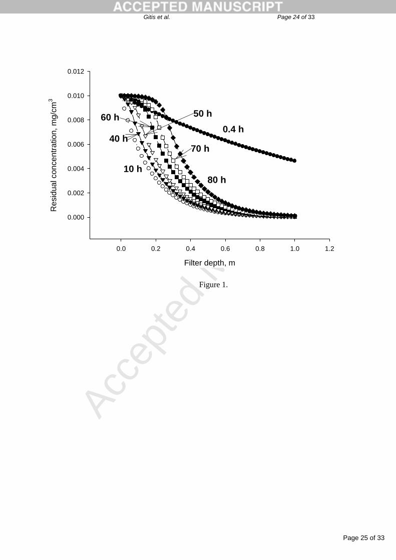
Figure 1 shows the local concentration as a function of the depth for various instants ranged from

24 min (0.4 h) to 80 h. The observed curves can be subdivided into three cases: an almost linear

decrease from the entrance to the column, observed at 0.4 h; an exponential decrease from the

entrance to the column, observed at 10, 40, 50 and 60h; and an exponential decrease which starts

Page 14 of 33

Accep

ted

Man

uscr

ipt

Gitis et al. Page 13 of 33

somewhere inside the column, observed at 70 and 80h. Here, the linear decrease at 0.4 h corresponds

to the first, irreversible, filtration stage that is characterized by minor changes in the deposit along the

filter. The curves at 10, 40, 50 and 60h correspond to the second, operable, filtration stage for the

entire filter. Here, the specific deposit value exceeds r = 0.2 mg/cm3 but does not reach u = 20

mg/cm3. Finally, the curves for 70 and 80 hours correspond to a situation in which a significant

amount of the sediment had been accumulated in the filter. As a result, no changes in the residual

concentration are observed in the filter part located close to the entrance. In Fig. 1, the depths of 0.2

and 0.3 m, for 70 h and 80 h respectively, have only a minor effect on the residual concentration. This

observation corresponds to the specific deposit saturation, u, achieved at a given depth, meaning that

that the corresponding part of the filter only transfers the particles while their concentration is not

affected.

The corresponding changes in the specific deposit, σ, as a function of bed depth for various instants,

are depicted in Fig. 2. The presented data allow direct tracking of the three-stage deposition kinetics.

For example, the plot shows that the specific deposit at 0.4 h is lower than r = 0.2 mg cm-3

and,

accordingly, the deposition evolves slowly. At 10, 20, and 30 h of filtration, the rate of deposition

increases yet the entire filter is in the operable stage. After 30 hours, the retention capacity of the top

5 cm layer exceeds the set u level of 20 mg cm-3

. Referring to Fig. 1, this means that the residual

concentration in the upper 5 cm of the filter does not change. The deeper-lying layers of the column

are taken out of action one after the other. As a result, the retaining effect of the column deteriorates.

This is reflected in a gradual increase in the residual concentration at a given location within the

column, which lasts until the concentration at that location is the same as at the entrance, meaning that

the entire part of the column between the entrance and the location concerned is saturated.

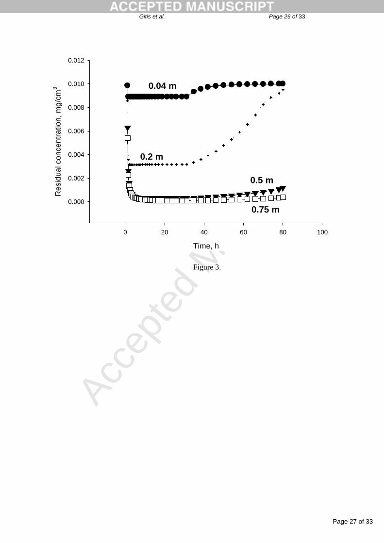
Figure 3 shows the concentration vs. time, while the depth serves as the parameter. One can see

that for any given depth, the concentration first decreases steeply, then remains practically constant,

and finally increases back to its maximum value. Actually, the first stage precedes the steep decrease,

which indicates that the transition to reversible accumulation has begun. The curves for different

Page 15 of 33

Accep

ted

Man

uscr

ipt

Gitis et al. Page 14 of 33

depths are similar, but it is obvious that deeper into the column lower concentrations are reached, and

this is because of filtration by a thicker bed. For any depth, the concentration eventually attains the

same value as at the entrance, but this happens much later for deeper locations. As follows from

Fig. 4, the deposit at any given depth also reaches its maximum value eventually, first close to the

entrance and then throughout the filter towards the exit.

Figure 5 shows an effect of the detachment-attachment ratio, Kd/Ka, on the concentration at the exit.

It is obvious that the lower this ratio, the lower the concentration achieved, and the longer the time for

which the concentration remains at its minimum. Thus, Figs. 1-5 indicate that the model yields

physically-meaningful predictions of well-established filtration stages [16].

5. Comparison with experiments

Two types of comparisons are presented in Figs. 6-9, and this in order to demonstrate the ability of

the model to predict the filtration results under a broad variety of experimental conditions. Figures 6

and 7 present the laboratory experiments, whereas the results of Figs. 8 and 9 have been obtained in

field experiments performed by the Mekorot Water Company at Eshkol site [35].

The experiments reflected in Figures 6 and 7 have been performed by Gitis [36, 37] at U.S. EPA

Test and Evaluation (T&E) Facility in Cincinnati, Ohio. A special pilot-scale filtration system was

designed and built. A 2.6 m high, 0.17 m in diameter acrylic transparent filter column had 9 sampling

and 9 pressure ports, located in pairs from opposite sides of the column. Sampling points were

inserted 0.05 m inside the column to avoid wall effect that misinterprets filtrate quality. The column

was packed with 1.6 m of uniform size sand having geometric mean diameter of 1.05 mm and

uniformity coefficient of 1.55. The media porosity, determined by volumetric measurements, was

0.44. The size and characteristics of the set-up were chosen in order to reflect practical filtration

conditions. In particular, the filter had to be deep enough to allow the overall filtration parameters to

be valid. On the other hand, the above mentioned nine 9 sampling and 9 pressure ports allowed to

monitor smaller depths during the same runs.

Page 16 of 33

Accep

ted

Man

uscr

ipt

Gitis et al. Page 15 of 33

A slurry, which consisted of Kaolin clay particles and Cincinnati tap water, was pumped into a

1000 L Cross-Linked Polyethylene (XLPE)-made feed tank. Suspension in the tank was kept

completely mixed by using a high-speed mixer. A centrifugal pump was used to lift the suspension

into a 100 L head tank located 3.6 m above the filtration column. Water level in the feed tank was

maintained at a constant height by an overflow line returning the suspension to the feed tank. The

column was operated at a constant flow rate of 5 and 10 m/h, under the contact (in-line) filtration

mode in the conventional downward direction. The filtration velocity was controlled and adjusted by

a flowmeter connected to the column outlet. Immediately after each run, filter was backwashed for

1 minute by air flow at 200 kN/m2, and then for 10 minutes by a reversed flow of Cincinnati tap water

at 1.1 L/sec.

Figures 6 and 7 show the residual concentration evolution at three different bed depths: 0.82, 1.02

and 1.62 m, for two different experimental runs. A typical numerical run takes about an hour and a

half on a PC, which may be considered as relatively fast. One can see that a reasonable agreement is

achieved between the model predictions and the experiments, with the following values of model

parameters: Kr = 2.5 and 1.2 1/m, Ka = 9 and 7.5 1/m, r = 0.35 and 0.2 mg/cm3 for Figs. 6 and 7,

respectively, Kd = 0.005 1/h, u=10 m/h, and u = 20 mg/cm3. In particular, the first two stages of

filtration, irreversible and operable, are clearly observed. It can be seen that, although an explicit

scheme is used, no oscillating or non-monotonic profiles are encountered. We note that the runs were

not sufficiently long to achieve the third, breakthrough, stage.

In Fig. 8, the model is compared to two different field experiments. The filtration velocity is

25m/hour. One can see that a good agreement between the predictions and the experimental results is

achieved for the entire filtration process with the following parameters: u = 25 m/h, L = 1.7 m,

Kr = 0.5-0.7 1/m, Ka = 8.5-9 1/m, Kd = 2·10-3

1/h, r = 0.1 mg/cm3, u = 9.5-10.2 mg/cm

3. In particular,

it appears that the model predicts the late stage of the process rather accurately.

In Fig. 9, the model is compared to the field experiments represented by two different runs in the

same filtration column. Again, a good agreement is observed. It is worth to note that the values of the

Page 17 of 33

Accep

ted

Man

uscr

ipt

Gitis et al. Page 16 of 33

parameters used in the simulations are the same as in Fig. 8, except for Ka and u, which also are

rather close (9 vs. 7 and 10.2 vs. 12.5, respectively). These differences, which probably reflect

variations that exist in the industrial system used in the experiments, do not contradict to the general

applicability of the model presented herein.

6. Conclusions

In the present study, a phenomenological model of deep-bed filtration is suggested. It combines an

advection-dispersion equation with an equation of nonlinear multistage accumulation kinetics. It is

assumed that at any location inside the column, the filter deposit is formed first as an irreversible

ripening layer, followed by the formation of a reversible deposit during the operable stage. The latter

continues until the deposit reaches locally its maximum value. Then, filter breakthrough takes place.

Thus, the suggested model is able to represent the entire filtration cycle. The model also includes

dispersion and accounts for temporal and spatial changes in media porosity.

The equations have been solved numerically, using an explicit finite-difference scheme. The

parameter values were set in the ranges reported in the literature. Time and space dependence of the

residual concentration and specific deposit are revealed. Furthermore, predictions of the model are

compared with the available experimental data. The results are in a good agreement with both

laboratory experiments at a U.S. EPA facility and field experiments performed by Mekorot – Israeli

Water Company.

The calculations suggest that the major parameters of the model, which determine the general

shape of the filtration curves, are the attachment rate constant, Ka, and the lower and upper deposit

thresholds of the reversible accumulation stage, r and u, respectively. At the same time, the other

two parameters of the kinetic model, namely the primary accumulation rate, Kr, and the detachment

rate, Kd, have relatively minor effects at standard filtration conditions.

Page 18 of 33

Accep

ted

Man

uscr

ipt

Gitis et al. Page 17 of 33

7. Acknowledgements

This research was supported by the Israel Science Foundation (grant No. 1184/06). We thank

Dr. Samir Hatukai for pilot filtration data.

Page 19 of 33

Accep

ted

Man

uscr

ipt

Gitis et al. Page 18 of 33

8. References

[1] Cleasby J.L., Logsdon G.S. (1999) Granular bed and precoat filtration. In Letterman R.D. (ed.)

Water quality and treatment: a handbook of community water supplies, AWWA (5th

edition),

McGraw-Hill, New York.

[2] Iwasaki T. (1937). Some notes on sand filtration. Journal of American Water Works Association,

29 (5), 1591-1602.

[3] Minz D. M. (1951). Kinetics of filtration of low-concentration water suspensions in water

purification filters. Doklady Akademii Nauk SSSR, 78, 315-318, in Russian.

[4] Amirtharajah A. (1988) Some theoretical and conceptual views of filtration. Journal American

Water Works Association 80, 36-46.

[5] Ives K.J. (1970) Rapid filtration. Water Research 4, 201-223.

[6] Tien C., Ramarao B.V. (2007) Granular filtration of aerosols and hydrosols. 2nd

edition, Elsevier.

[7] Guedes R.G., Al-Abduwani F., Bedrikovetsky P., Currie P.K. (2009) Deep-bed filtration under

multiple particle-capture mechanisms. Society of Petroleum Engineers Journal 14, 477-487.

[8] Zamani A., Maini B. (2009) Flow of dispersed particles through porous media - deep bed filtration.

Journal of Petroleum Science and Engineering 69, 71-88.

[9] Alvarez A.C., Hime G., Marchesin D., Bedrikovetsky P. (2007) The inverse problem of

determining the filtration function and permeability reduction in flow of water with particles in

porous media. Transport in Porous Media 70, 43-62.

[10] Vigneswaran S., Ben Aim R. (1989) Water, wastewater and sludge filtration. CRC Press, Boca

Raton, Florida, USA.

[11] Ives K. J. (1969) Theory of filtration. Special Lecture No.7 in Proceedings of the International

Water Supply Association, Eight Congress, Vienna, 1, K3-K28.

[12] Herzig J.P., Leclerk, D.M., Le Goff P. (1970). Flow of suspensions through porous media-

application to deep filtration. Industrial Engineering Chemistry, 62 (5), 8-35.

[13] O'Melia C.R., Ali W. (1978). The role of retained particles in deep bed filtration. Progress in

Water Technology, 10 (5/6), 167-182.

Page 20 of 33

Accep

ted

Man

uscr

ipt

Gitis et al. Page 19 of 33

[14] Tien C., Turian R.M., Pendse H. (1979) Simulation of the dynamic behavior of deep bed filters.

Journal of American Institute of Chemical Engineers, 25 (3), 385-395.

[15] Adin A., Rebhun M. (1977). A model to predict concentration and head-loss profiles in filtration.

Journal of American Water Works Association, 69 (8), 444-453.

[16] Crittenden J.C. (ed.) (2005) Water Treatment: Principles and Design. Wiley, 2nd

edition.

[17] Ives K.J. (1973) Capture mechanisms in filtration in The Scientific Basis of Filtration, Part II,

Chapter 9. NATO Advanced Study Institute, Cambridge, England.

[18] Adin A., Rebhun M. (1987) Deep-bed filtration: accumulation-detachment model parameters.

Chemical Engineering Science, 42(5), 1213-1219.

[19] Gitis V., Adin, A., Rubinstein, I. (1999). Kinetic models in rapid filtration. Procedures of

American Water Works Association Annual Conference, 1999, Chicago, IL.

[20] Payatakes A. C., Tien C. (1976). Particle deposition in fibrous media with dendrite-like pattern:

a preliminary model. Journal of Aerosol Sciences, 7, 85-100.

[21] Ziskind G. (2006) Particle resuspension from surfaces: Revisited and re-evaluated. Reviews in

Chemical Engineering 22, 1-123.

[22] Baylis J. R. (1937) Experiences in filtration. Journal of American Water Works Association, 29

(12), 1010-1048.

[23] Baumann E.R., Ives K.J. (1982). The evidence for wormholes in deep bed filters. Proc. Filtech

conf. Utrecht, 1, 151-164.

[24] Yao K. M., Habibian M. T., O’Melia C. R. (1971). Water and wastewater filtration: concepts and

applications. Environmental Science and Technology 5 (11), 1105-1112.

[25] Danckwerts P.V. (1953) Continuous flow systems. Distribution of residence times. Chemical

Engineering Science, 2 (1), 1-13.

[26] Rubinstein I., Rubinstein L. Partial differential equations in classical mathematical physics.

Cambridge University Press, Canada, 1993.

[27] Edwards C.H., Penney D.E. (1999) Differential Equations: Computing and Modeling, 2nd

Edition, Prentice-Hall College Div, Inc. Pearson Education Upper Saddle River, New Jersey, USA

Page 21 of 33

Accep

ted

Man

uscr

ipt

Gitis et al. Page 20 of 33

[28] Chapra S.C. (1997) Surface water-quality modeling. McGraw-Hill, New York.

[29] Atkinson J.F., Gupta S.K., DePinto J.V., Rumer R.R. (1998) Linking hydrodynamic and water

quality models with different scales. Journal of Environmental Engineering – ASCE, 124(5),

399-408.

[30] Bear J., Verruijt A. (1987) Modeling groundwater flow and pollution. Kluwer Academic

Publishers, Dordrecht, Holland.

[31] Vigneswaran S., Tulachan K.R. (1988) Mathematical modeling of transient behavior of deep bed

filtration. Water Research, 22 (9), 1093-1100.

[32] Choo C.U., Tien C. (1995) Simulation of hydrosol deposition in granular media. AICHE Journal

41, 1426-1442.

[33] Rajagopalan R., Tien C. (1976) Trajectory analysis of deep-bed filtration with the sphere-in-cell

porous media model. AIChE Journal 2, 523-533.

[34] Rajagopalan R., Chu R.Q. (1982) Dynamics of adsorption of colloidal particles in packed-beds.

Journal of Colloid and Interface Science, 86 (2), 299-317.

[35] Hatukai S., Gavron E. (1996). Filtration pilot plant for Israelis national water carrier.

International Water & Irrigition Review, 16 (3), 14-19.

[36] Gitis V. (2001) Removal of oocysts of Cryptosporidium parvum by rapid sand filtration. Annual

Project Report, IT Corporation for U.S. EPA, Contract No. 68-C-99-211, 104 pp.

[37] Gitis V. (2008) Rapid Sand Filtration of Cryptosporidium parvum: Effects of Media Depth and

Coagulation. Water Science & Technology – Water Supply 8 (2), 129-134.

[38] Camp T. R. (1964) Theory of water filtration. Proc. Am. Soc. Civil Engng 90 (SA4) paper 3990.

[39] Vigneswaran S., Chang J. S. (1989) Experimental testing of mathematical models describing the

entire cycle of filtration. Water Research, 23 (11), 1413-1421.

[40] Osmak S., Glasnovic A. (1994) The study of filter coefficient behavior using attachment -

detachment model for deep bed filtration. Chemistry and Biochemistry Engineering Quarter, 8 (4),

177-181.

[41] Deb A.K. (1969) Theory of sand filtration. J. Sanitary Eng. Div., ASCE, 95, 399-422.

Page 22 of 33

Accep

ted

Man

uscr

ipt

Gitis et al. Page 21 of 33

[42] Shechtman Yu.M. (1961) Filtration of low-concentration suspensions. Izdat.Akad.Nauk SSSR,

Inst.Mekhaniki, Moscow (in Russian).

[43] Mackie R.I., Horner R.M.W., Jarvis R.J. (1987) Dynamic modeling of deep-bed filtration.

Journal of American Institute of Chemical Engineers, 33 (11), 1761-1775.

[44] Ojha C.S.P., Graham N.J.D. (1993) Theoretical estimates of bulk specific deposit in deep bed

filters. Water Research 27, 377-387.

[45] Gontar Yu.V. (1987) A modified model of water clarification in filtration through porous media.

Khim. Tekhnol. Vody 9, 487-490 (in Russian).

Page 23 of 33

Accep

ted

Man

uscr

ipt

Gitis et al. Page 22 of 33

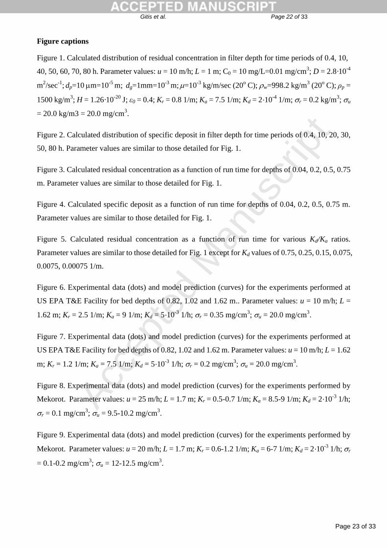
Figure captions

Figure 1. Calculated distribution of residual concentration in filter depth for time periods of 0.4, 10,

40, 50, 60, 70, 80 h. Parameter values: u = 10 m/h; L = 1 m; C0 = 10 mg/L=0.01 mg/cm3; D = 2.8·10

-4

m2/sec

-1; dp=10 m=10

-5 m;

dg=1mm=10

-3 m;

=10-3

kg/m/sec (20o C); w=998.2 kg/m

3 (20

o C); ρp =

1500 kg/m3; H = 1.26·10

-20 J; ε0 = 0.4; Kr = 0.8 1/m; Ka = 7.5 1/m; Kd = 2·10

-4 1/m; r = 0.2 kg/m

3; u

= 20.0 kg/m3 = 20.0 mg/cm3.

Figure 2. Calculated distribution of specific deposit in filter depth for time periods of 0.4, 10, 20, 30,

50, 80 h. Parameter values are similar to those detailed for Fig. 1.

Figure 3. Calculated residual concentration as a function of run time for depths of 0.04, 0.2, 0.5, 0.75

m. Parameter values are similar to those detailed for Fig. 1.

Figure 4. Calculated specific deposit as a function of run time for depths of 0.04, 0.2, 0.5, 0.75 m.

Parameter values are similar to those detailed for Fig. 1.

Figure 5. Calculated residual concentration as a function of run time for various Kd/Ka ratios.

Parameter values are similar to those detailed for Fig. 1 except for Kd values of 0.75, 0.25, 0.15, 0.075,

0.0075, 0.00075 1/m.

Figure 6. Experimental data (dots) and model prediction (curves) for the experiments performed at

US EPA T&E Facility for bed depths of 0.82, 1.02 and 1.62 m.. Parameter values: u = 10 m/h; L =

1.62 m; Kr = 2.5 1/m; Ka = 9 1/m; Kd = 5·10-3

1/h; r = 0.35 mg/cm3; u = 20.0 mg/cm

3.

Figure 7. Experimental data (dots) and model prediction (curves) for the experiments performed at

US EPA T&E Facility for bed depths of 0.82, 1.02 and 1.62 m. Parameter values: u = 10 m/h; L = 1.62

m; Kr = 1.2 1/m; Ka = 7.5 1/m; Kd = 5·10-3

1/h; r = 0.2 mg/cm3; u = 20.0 mg/cm

3.

Figure 8. Experimental data (dots) and model prediction (curves) for the experiments performed by

Mekorot. Parameter values: u = 25 m/h; L = 1.7 m; Kr = 0.5-0.7 1/m; Ka = 8.5-9 1/m; Kd = 2·10-3

1/h;

r = 0.1 mg/cm3; u = 9.5-10.2 mg/cm

3.

Figure 9. Experimental data (dots) and model prediction (curves) for the experiments performed by

Mekorot. Parameter values: u = 20 m/h; L = 1.7 m; Kr = 0.6-1.2 1/m; Ka = 6-7 1/m; Kd = 2·10-3

1/h; r

= 0.1-0.2 mg/cm3; u = 12-12.5 mg/cm

3.

Page 24 of 33

Accep

ted

Man

uscr

ipt

Gitis et al. Page 23 of 33

Table 1. Parameter values used in the test runs

Parameter Units The

range

The references

Initial porosity - 0.4 0.41 [38]

0.39 [39]

0.35 [40]

Attachment rate coefficient in the

ripening stage

Kr 1/m 0.8-2.5 3.1 [32]

1.5 [33]

Attachment rate coefficient in the

operable stage

Ka 1/m 6-9 10-12 [41]

5-12 [42]

12-15 [15]

3-150 [40]

10-90 [43]

20-30 [44]

Detachment rate coefficient in the

operable stage

Kd 1/h 2·10-4

-

2·10-3

1.5·10-4

-2·10-4

[42]

1.5·10-3

[45]

1.3·10-6

[15]

2.2·10-5

-1.6·10-3

[40]

Transient specific deposit σr mg/cm3 0.1-0.35

Ultimate specific deposit σu mg/cm3 9.5-20 130 [14]

42-60 [39]

20-70 [15]

Page 25 of 33

Accep

ted

Man

uscr

ipt

Gitis et al. Page 24 of 33

Filter depth, m

0.0 0.2 0.4 0.6 0.8 1.0 1.2

Re

sid

ua

l co

ncentr

ation, m

g/c

m3

0.000

0.002

0.004

0.006

0.008

0.010

0.012

0.4 h

80 h

70 h

60 h 50 h

40 h

10 h

Figure 1.

Page 26 of 33

Accep

ted

Man

uscr

ipt

Gitis et al. Page 25 of 33

Filter depth, m

0.0 0.2 0.4 0.6 0.8 1.0 1.2

Specific

deposit, m

g/c

m3

0

5

10

15

20

25

0.4 h

10 h

20 h

30 h

50 h

80 h

Figure 2.

Page 27 of 33

Accep

ted

Man

uscr

ipt

Gitis et al. Page 26 of 33

Time, h

0 20 40 60 80 100

Re

sid

ual co

ncentr

ation, m

g/c

m3

0.000

0.002

0.004

0.006

0.008

0.010

0.012

0.04 m

0.75 m

0.5 m

0.2 m

Figure 3.

Page 28 of 33

Accep

ted

Man

uscr

ipt

Gitis et al. Page 27 of 33

Time, h

0 20 40 60 80 100

Specific

deposit, m

g/c

m3

0

5

10

15

20

25

0.04 m 0.2 m

0.5 m

0.75 m

Figure 4.

Page 29 of 33

Accep

ted

Man

uscr

ipt

Gitis et al. Page 28 of 33

Kd/Ka ratio

Run time, h

0 20 40 60 80 100

Resid

ual concentr

ation, m

g/c

m3

0.000

0.002

0.004

0.006

0.008

0.010

0.012

0.1

3x10-2

2x10-2

10-2

10-3

10-4

Figure 5.

Page 30 of 33

Accep

ted

Man

uscr

ipt

Gitis et al. Page 29 of 33

Time, h

0 2 4 6 8

Resid

ual ra

tio C

/C0

0.00

0.05

0.10

0.15

0.20

0.25

Bed depth

0.82 m

1.02 m

1.62 m

Figure 6.

Page 31 of 33

Accep

ted

Man

uscr

ipt

Gitis et al. Page 30 of 33

Time, h

0 2 4 6 8 10

Re

sid

ua

l ra

tio C

/C0

0.0

0.1

0.2

0.3

0.4

0.5

0.6Bed depth

0.82 m

1.02 m

1.62 m

Figure 7.

Page 32 of 33

Accep

ted

Man

uscr

ipt

Gitis et al. Page 31 of 33

0

0.1

0.2

0.3

0.4

0.5

0 10 20 30 40

Run time, h

Re

sid

ua

l ra

tio

C/C

0

Run78

Run76F

Figure 8.

Page 33 of 33

Accep

ted

Man

uscr

ipt

Gitis et al. Page 32 of 33

0

0.1

0.2

0.3

0.4

0.5

0 10 20 30 40

Run time, h

Re

sid

ua

l ra

tio

C/C

0

Run71F

Run71D

Figure 9.