Retrospective Theses and Dissertations Iowa State University Capstones, Theses andDissertations

1960

Development of multistage designs for statisticalsurveys in the PhilippinesBurton Torres OnateIowa State University

Follow this and additional works at: https://lib.dr.iastate.edu/rtd

Part of the Statistics and Probability Commons

This Dissertation is brought to you for free and open access by the Iowa State University Capstones, Theses and Dissertations at Iowa State UniversityDigital Repository. It has been accepted for inclusion in Retrospective Theses and Dissertations by an authorized administrator of Iowa State UniversityDigital Repository. For more information, please contact digirep@iastate.edu.

Recommended CitationOnate, Burton Torres, "Development of multistage designs for statistical surveys in the Philippines" (1960). Retrospective Theses andDissertations. 2624.https://lib.dr.iastate.edu/rtd/2624

DEVELOPMENT OF MULTISTAGE DESIGNS

FOR STATISTICAL SURVEYS IN THE PHILIPPINES

"by

Burton Torres Onate

A Dissertation Submitted to the

Graduate Faculty in Partial Fulfillment of

The Requirements for the Degree of

DOCTOR OF PHILOSOPHY

Major Subject: Statistics

Approved:

Dean of Graduate College

Iowa State University Of Science and Technology

Ames, Iowa

1960

Signature was redacted for privacy.

Signature was redacted for privacy.

Signature was redacted for privacy.

11

TABLE OF CONTENTS

Page

I. INTRODUCTION 1

II. REVIEW OF LITERATURE 9

A. Related Specifications of the Sampling System 9

1. Sampling unit and hierarchy of sampling unit 9

?.. Some procedures of selection of sample. 1-3 3. Some methods of estimation 17

3. Problems in Sampling for Time Series. ... °3

III. SAMPLE DESIC-N ?9

A. Background Data °9

1. Location and area °9 ?.. Population 30 3. Political subdivision 30

B. Samrle Design 31

1. Regional stratification 31 ?.. Stratification within region 3? 3. Methods of sample selection 33 4. Multi-stage sampling with complete

replacement of primaries 39 5. Details of methods of estimation. ... 4?

C. Comparison of 1 Survey1 and 1 Stratified1

Estimates of Variance 63

IV. ROTATION OF SAMPLE 65

A. Development of a Rotation Scheme 65

1. Purpose 65 ?.. Description of the new rotation scheme. 68

B. Sampling Rate within Segments 70

1. Equal sampling rate 7? ?. Unequal sampling rate 84

ill

Page

V. RATIO ESTIMATION 94

A. Control of the Variation in the Size of Barrio 95

B. Ratio Estimation in the Urban Area 10-3

1. Biased ratio estimation 104 ?. Unbiased ratio estimation 1°1

C. Empirical Results 130

VI. COMPOSITE ESTIMATION 147

A. Estimate of Stratum Total, ^^th» fr0m

the i^*1 Primary 148

1. Structure 148 ?. Variance 150

B. Estimate of Visit-to-Visit Change, e(xth - ai -lXth » from the 1th Primary . . . 158

1. Structure 158 2. Variance 159

C. Estimate of Visit-to-Visit a Year Ago Change, from the

ith Primary 16?

1. Structure 16° ?. Variance 163

D. Sector Estimate 165 E. Choice of an Appropriate Q 168 F. Finite Population Approach 170

1. Structure of estimate 179 P. Variance of composite estimate 177

VII. SUMMARY AND RECOMMENDATIONS 191

VIII. LITERATURE CITED 199

IX. ACKNOWLEDGMENT P O P

1

I. INTRODUCTION

From the time of her discovery by Spain in 1521, to the

year of her independence in 1946, the Philippines had expe­

rienced three important historical periods. She was under

the Spanish colonial regime from 1521 to 1900; the American

administration from 1900 to 1941; and under the Japanese

military occupation from 1941 to 1945. Shortly after World

War II, she became an independent republic on July 4, 1946.

No major statistical activity was conducted prior to

1900. Censuses of population and selected characteristics of

socio-economic life in the Philippines were conducted under

American administration in 1903, 1918, 1939, but without the

help and support of a general purpose statistical organiza­

tion.

The present Bureau of the Census and Statistics was

created in 1940, under the office of the President, by Common­

wealth Act No. 591 which transferred powers, functions,

duties, personnel, appropriations, property and records from

various offices of the Commonwealth Government to the new

Bureau, effective January 1, 1941. Little could be done by

the new Bureau until after the Japanese occupation. A

national census of population and agriculture was taken in

1948 under the auspices of the new Bureau. On February, 1951,

the Bureau was transferred to the Department of Commerce and

Industry.

2

The idea of centralization of government statistics which

was reflected in the Bureau's set-up, has not been workable on

a government-wide basis, and statistical activities soon re­

appeared in the other offices and departments of the govern­

ment . The pattern thus became one of decentralization, with

each office or department active in the statistical operations

for its own administrative purposes, while the Bureau of the

Census and Statistics serves as the specialized multipurpose

statistical office.

During the past few years, the importance of statistics

for government and private use, in the Philippines, has re­

ceived growing recognition. This is reflected in a widespread

growth of statistical activities in all echelons of the gov­

ernmental system and also in the production of basic informa­

tion on the population and socio-economic life of the country

necessary for economic development programs. This recognition

is basically reflected in the legal provisions which have set

a framework for the administration of a coordinated statistical

program and for the improvement of statistical standards.

The Government Survey and Reorganization Commission

created by Republic Act No. 997, 1952, recommended, among

others, that the present system of decentralized statistical

operations should be continued and that a central office be

created to coordinate this decentralized system. To Implement

these recommendations, the Office of Statistical Coordination

3

and Standards8 (OSCAS) was created under the revitalized

National Economic Council (NEC) by Executive Order No. 119,

July 1, 1955 and the OSCAS was formally organized January 1,

1956. This office is charged with the responsibility to:

(a) promote an orderly and efficient program to meet the

statistical requirements of the government, especially the

NEC; (b) develop and prescribe adequate standards and methods

for the use of other statistical agencies; and (c) maintain

effective coordination of decentralized statistical activ­

ities. Within this new framework of statistical organization,

several inter-departmental committees have been set up to

study the best allocation of responsibilities for collecting

data in fields where serious duplications existed and the

Improvements of standards and methods for various types of

data.

The OSCAS has realized that with a fast growing and

dynamic population even a complete census at various inter­

vals, say five or ten years, is of limited use. Data from

the census of 1948, for example, will not be very useful in

the preparation of the NEC five-year economic and social

development programs which require a thorough knowledge of the

socio-economic characteristics of the population in 1956. Data

obtained from a series of sample surveys conducted every year

aThe author is Assistant Director of this new office.

4

or every six months will be more useful.

One of the most important results of these considerations

was the creation and organization of a national sample survey,

The Philippine Statistical Survey of Households (PSSH), which

was started in May, 1956 under the direct administrative and

technical supervision of the OSCAS and with the cooperation of

the Bureau of the Census and Statistics as the operating agency.

The PSSH was organized for the purpose of (a) obtaining on a

sample basis up-to-date statistical data on the size, composi­

tion and distribution of the population, labor force, economic

activities of the people, income and expenditures, toilet and

water facilities and other related information; and (b) main­

taining these statistics on a current basis.

The PSSH utilized the sub-sampling technique, commonly

known as multi-stage sampling. This technique is especially

valuable in a country like the Philippines where no adequate

frames exist. As mentioned earlier, the last census was con­

ducted In 1948. Multi-stage sampling enables the complete

utilization of existing political or administrative divisions

such as provinces, towns or municipalities, and barrios in the

rural sector and precincts in the urban sector of the country

as sampling units at various stages. This technique permits

also the permanent concentration of field work at various

primary or secondary sampling units scattered throughout the

country. The time of the supervisor assigned in each region

5

will be spent efficiently for training and supervision instead

of travelling and locating the interviewers. Another advantage

is the fact that the construction of the frame for succeeding

stages need only be carried out for those previous stage units

which are actually included in the sample. One of the most

important requirements of the present design of the PSSH is

the complete listing of households in certain sampling units.

The structure of the present design of the PSSH, and the

operations involved in each stage will be discussed in Chapter

III. It will also be shown how some of the design details have

been obtained as 1 optimum solutions' subject to the limitations

Imposed by local conditions and resources. Formulas for the

estimation of population totals and sector totals are given and

formulas for estimating their variances are discussed.

The present PSSH is a 1 panel survey1 as far as certain

sampling units (areas) are concerned - and once put into opera­

tion commits the estimation procedures to the permanent design.

The choice of technical devices Is limited to a redefinition

of the sampling units, to different methods of sampling within

the selected primary or secondary sampling units, to the

choice of the estimation procedure, or to the use of tech­

niques which will result in the reduction of the cost of the

survey. Such Improvements in the design of the PSSH through

the use of these various techniques will be presented in

Chapters IV, V and VI.

6

The design and estimation procedure of the PSSH require

the complete listing of the ultimate clusters or sampling

areas. This first phase of the field operation is done about

one week prior to actual interviewing of the sample households

and consists of a complete enumeration of all households,

population in households and occupation of head in each of the

designated sampling areas. About 0.163 million households and

0.969 million population are listed during this first phase of

each survey or visit. These figures give an idea of the ex­

tent and possible cost of the listing operation alone. More

than 15 per cent of the field cost is devoted to this opera­

tion. Since the PSSH was devised to sample the same popula­

tion repeatedly, another important point which has to be con­

sidered is the frequency of visit to the panel households and

the pattern in which the sample will have to be changed from

visit to visit. It has been observed that heads of households

or the respondents have become uncooperative during the third

or fourth visit. This brings up the question of 1 response re­

sistance1 . Even with complete cooperation, the respondents

may also be influenced by the information which they give

and receive during the Interviews, and this constant exposure

may make them progressively less representative in succeeding

visits. A rotation scheme will be developed in Chapter IV

which will provide some answers to the problem of cost of

listing and to the question of 1 response resistance' of panel

7

households.

An attempt was made to equalize the size of the barrio

sector in the barrio stage. This development will be described

and some empirical results will be given to indicate the

effect of equalization. In addition, ratio estimation with

rotation will be introduced into the estimation procedure.

These techniques are described in Chapter V.

The rotation scheme for the 'matched sample1 design

developed in Chapter IV consists of changing a portion of the

sample of households from visit to visit. This situation

affords an excellent opportunity to use a new estimation pro­

cedure, the so-called composite estimate (Chapter VI), a sim­

ilar version of which is used by the U. S. Bureau of the Census

in their current population survey. For the preparation of

socio-economic development plans, the interest is on the cur­

rent total, particularly for data or characteristics of the

population which are likely to change considerably with time.

A composite estimate will be developed which will estimate

the current total or level.

The NEC development programs are revised from year to

year consistent with the performance attained and with what­

ever modifications changing conditions may warrant. In order

to evaluate the effects of these programs on the various sec­

tors of the economy, estimate of change is of prime importance.

For this situation, the composite estimate for each succeeding

8

visit will be utilized to give an estimate of the visit-to-

visit change and an estimate of the visit-to-visit a year

ago change. The gain in reliability of these estimates will

also be discussed.

9

II. REVIEW OF LITERATURE

The review of literature will consist of two main head­

ings, namely: (a) related specifications of the sampling

system; and (b) problems arising when sampling time series

with panel households. The first will have special bearing on

the developments given in Chapters III, IV and V; the second

on Chapters IV and VI.

A. Related Specifications of the Sampling System

The requirements of an efficient sampling system are many

and varied. These include, among others, the definition of

the sampling unit, the method of selecting the elements or

sampling unit which will constitute the sample and the method

of estimation to be used. Techniques have been devised for

the utilization of auxiliary information, quantitative or

qualitative, to improve these requirements of the sampling

system.

1. Sampling unit and hierarchy of sampling units

The definition of the sampling unit (su) in any sampling

system is of great importance. It is a concept subject to con­

siderable choice. In practice, It is often possible to sub­

divide the population into sampling units (sus) in many ways.

An urban area may be regarded as composed of a number of pre-

10

clncts (voting areas), or of a number of blocks, or of a num­

ber of households, or of a number of persons. In multi-stage

designs, the precincts may be used as the first stage units,

the blocks as second stage units, the households as third

stage units and the persons as the fourth stage units. In

this way, one can create a hierarchy of sampling units.

Jessen jlôj investigated the efficiencies of four sizes

of units in sampling for farm facts. He compared a quarter

section, a half section, a section (area of 1 square mile),

and a block of two contiguous sections. In most of the items

studied the quarter section was found to be optimum. In India,

Sukhatme and Panse [29j| considered the village as the optimum

unit of sampling in agricultural surveys. The village is also

a very convenient administrative subdivision.

With auxiliary information, one can define units which

are as alike as possible with regard to one or more character­

istics under study. This technique will result in an increase

of efficiency of a sampling system with equal probability due

primarily in a reduction of the variance of the individual

units. Another method is to use clusters, aggregates, or

groups of natural units as sus. The use of these sus is of

some appeal to countries where no accurate frame exists. Under

this method a sample of households may be obtained by asso­

ciating every household with one and only one areal segment

and then a sample of these areal segments is selected by some

11

random scheme. This is commonly known as area sampling.

Jeesen jl4^ introduced the use of auxiliary information in

the form of maps and aerial photographs in defining areal sus

which he found to be less variable in respect to the character­

istics under measurement than units of equal area.

Several attempts have been made to work out a relation

between the variance from a sample of sus of any size and the

variance from a sample of units of a specified size. The

effect on the variance of the estimate from using clusters

made up of varying numbers of elements as su's may be expressed

in terms of a measure S of homogeneity within su's ^9, Vol. 2,

p. 164j. Sukhatme ^28, p. 24?j discussed the efficiency of

cluster sampling in terms of the intra-class correlation.

For many items, $ tends to decrease with an increase of

the number of elements, but the rate of decrease is small

relative to the rate of increase in size. This relationship

may be expressed as

6 = * K

where K is the average number of elements per cluster, «£ Is a

positive constant and is a negative constant. If clusters

as sus are used rather than individual elements, then there is

usually an increase in the variance over that of simple random

sampling of the same number of elements by a factor

X = 1 + S(K - 1) .

In general, we expect the variance to Increase with the size of

12

the cluster. In some cases, however, clusters may be superior

to elements as sampling units. Sukhatme ^28, p. 248^ found

that households, as a cluster, will be approximately twice as

efficient as a single person for estimating the sex ratio.

In sub-sampling or multi-stage sampling plans where there

exists a hierarchy of sampling units, the different methods of

utilizing prior information are applicable at each stage of

sampling.

In order to increase the efficiency in a two-stage sam­

pling, Hansen and Hurwltz [s) recommended that strata be as

homogenous as possible and that strata be composed of large

primary internally heterogenous units. By increasing the

heterogeneity within primary sampling units (psus) the vari­

ability between psus was reduced, and on items for which this

component was large, considerable reduction in the total vari­

ance of the estimates was attained. Moreover, Dalenlus ^3,

p. 14j pointed out that for a constant number of secondary sus

in the sample, the total variance of the estimate will in­

crease on decreasing the number of psus In the sample. In gen­

eral multi-stage sampling, the type of psus usually has a much

greater impact on reduction of total variance of the estimate

than has the type of secondary sus. As a rule, the psus

should be made as internally heterogenous as possible, when

the primary sampling fraction is small.

There are ways other than changing the size of the peu in

13

•which heterogeneity within sus can be introduced and hence

variability between sus can be reduced. If certain administra­

tive or political units are being combined to form a peu, then

pairing of political units in which one is predominantly agri­

cultural and one which is largely urban, will introduce hetero­

geneity. More often, these units will depend upon the admin­

istrative or political subdivisions into which a given country

is segmented. In the United States, the county has been used

as a unit of sampling ^13, 2oj. The commune, smallest admin­

istrative unit, is used in the construction of the peu in the

Swedish national sample surveys ^3, p. lOôJ. Gray and Corlett

^6^ reported the use of districts as psus in most national

sample surveys in Britain. In the Philippines, the municipal­

ity, the second largest administrative unit in the rural area,

is used as psu while in the urban area the precinct or voting

area is used as psu. The reason for this choice is predomin­

antly of a practical administrative nature. It is possible

that the variation of certain items within a municipality is

smaller than the variation between municipalities in the same

stratum so that this unit as a psu may not be ideal from a

theoretical standpoint.

2. Some procedures of selection of sample

The availability of prior information on the elements of

the population will determine to a great extent the procedure

to follow in the selection of the units which will constitute

14

the sample. Procedures applicable to one-stage sampling may

be utilized at any stage of a hierarchy of sampling units.

In sinple random sampling n units are drawn out of N

units such that every one of the samples has an equal

chance of being chosen. As Is well known, the variance of a

sample mean Is Inversely proportional to the size of the sam­

ple. The precision of the sample mean is Increased by increas­

ing the size of sample n.

If prior Information is available about the N units, then

it may be possible to divide a heterogenous population of N

units Into sub-populations called strata of N^, Ng, ...,

units, each of which is Internally homogenous. Note that

strata should be homogenous while psus should be heterogeneous.

The sample is then allocated to each stratum (n^é: N^) and pre­

cise estimates are obtained from a smaller sample In each

stratum. These estimates can then be combined into a precise

estimate for the whole N population.

When the stratum sizes (N^1s) are known, the simplest

allocation is to make n% proportional to N%. For optimum

allocation of the sample in the respective strata with the

sample size

n- 2

make

nh h

15

where f % has different forms for different estimators. This

relation is often called 1Neyman1 allocation [22], although

this result was previously obtained by Tschuprow [soj . There

are, however, some practical difficulties associated in the use

of Neyman1 s method of allocation £2, p. 84j .

When strata sizes, %'s, are not known, as often happens

when stratum sizes are based on old census data which are out

of date for use in current surveys, the procedure given above

may still be utilized. A 1 large1 sample is first selected and

stratified into L strata and estimates of N^ are made; then

each stratum is considered as a sub-population. This procedure

is a special case of double sampling for stratification or two-

phase sampling. Double sampling may be very convenient when

the information about x^ is on file cards that have not been

completely tabulated. Cochran jl2, p. 268^ states that this

technique is profitable only if the gain in precision from

ratio or regression estimates or from stratification more than

offsets the loss in precision due to the reduction in the size

of the large sample.

Mahalanobis ^21^ states that an optimum or nearly optimum

solution to minimum variance stratification would be obtained

when the expected contribution of each stratum to the total

aggregate value of x^ is made equal for all strata. Hansen

£t al. ^9, Vol. 1, p. 416 j give a rule of thumb which will

provide a rough guide to the optimum sizes of strata when a

16

constant number of psus is selected from each stratum. The

rule is to make the strata equal in terms of X^, total of the

h^*1 stratum, when the psu rel-variances are about the same and

remain about the same on adjusting the sizes of strata.

Other methods of restriction, in addition to stratifica­

tion, may be introduced in the selection procedure. The pro­

cedure of first selecting psu and then selecting within each

psu a specified number of elements is known as sub-sampling or

multi-stage. As mentioned before, this procedure will group

the stage units into a hierarchal classification. The prin­

cipal advantage of multi-stage sampling is its greater flexi­

bility as compared to one-stage sampling. A balance between

administrative considerations, costs and precision dictate

that most sample surveys be of this type.

The selection of psu in a multi-stage design with com­

plete replacement of psu and with probability proportional to

size (pps) will be discussed in detail In Chapter III.

Systematic sampling consists of selecting a sample of

size n, by taking a unit at random from the first k units and

then every kth subsequent unit. Systematic samples are conve­

nient to draw and to execute £lj. When a list is used on

which the units are recorded in an essentially random way,

'systematic' samples are equivalent to random samples. When

such an assumption can not be made at least the random start

should be made. In such situations 'systematic1 samples with

17

a random start compare often favorably with stratified sam­

pling. The procedure is convenient especially in field opera­

tions. In this case, there is no gain in precision. This

type of sampling was utilized in the PSSH sample areas.

Available prior information can be used in any of the

operations which make up the sampling plan. This is done in

order to increase the precision of the overall results. This

information may be qualitative or quantitative. Some decision

will have to be made as to which of these information items

will be utilized for various operations of the survey such as

stratification, construction of psu1s, choice of the selection

procedure, choice of the estimation procedure and others.

3. Some methods of estimation

Another general use of prior information, usually quanti­

tative, arises in the estimation procedure. Its use will in

general give rise to an estimate of higher precision than can

be attained with estimators not utilizing this information.

In the succeeding discussions, the nomenclature usually

given by Hartley jllj for x, x and x* will be used.

The simplest estimation procedure may be called 1x only1

estimation. As estimate of the population mean, X, we define

as the 1x only1 estimator of X. Similarly, we may define y

as the 1 y only1 estimator of Y. If the quantitative informa-

18

tion, Y, Is known, then various ratio estimators may be used.

The 1 ratio of means' estimate js, p. 112; 1]^

~ = -1- Y y

is used to estimate X, where x and y are the 1x only' and

1 y only1 estimators of X and Y, respectively.

The 'mean of ratios' jll"] is another estimate of X and is

given as

x" = r Y

where

1

and

21 *i '

ri =

The familiar approximate formula for the variance of

'x and 1x |j2, p. 116; llj is

11 (Tx + Q2 ffy - Cov(x,y)j

where

x and x are biased j^2, p. 130; llj. In most surveys, the

bias may be a small portion of the standard deviation and may

be Ignored or neglected. In stratified sampling where the n%

in each stratum is email and L, the number of strata, is large,

19

the bias In the stratified total estimate may not be negligible

relative to its standard error. If the bias of the estimate

has the same sign in each stratum, then the bias in the esti­

mate of population total will be approximately L times that

for an individual stratum total, but the standard error is

only Yl times that for individual stratum total. Hartley and

•Ross £l2*J derived exact expressions for the bias in x and x

and from these results an unbiased ratio estimator, xl, was

worked out. This is given as

*• . ? Ï • îî-f-l (5 - ïy) .

Goodman and Hartley ^5™j compared the precision of x1 with that

of x and x. Results given in £2, 5, 11, isj will have direct

bearing in the introduction of ratio estimators into the de­

sign of the PSSH.

In the estimation of population total in multi-stage de­

signs, one of the most stringent requirements for an efficient

estimation procedure is an accurate knowledge of quantitative

characteristics of the various stage frames. The unbiased

estimate of the population total, X, in a three-stage design

without replacement and equal probability at each stage is

M è E r i j 1J k

where M Is the total number of psus in the population,

m is the number of sample psus,

20

Bj_ is the total number of secondary sus (ssus) in the

i**1 sample psu,

b^ is the number of sample ssus in the i^*1 sample psu,

Njj is the total number of listed households (hhs) in

the (ij)th sample ssu,

n^j is the number of sample hhs in the (ij)th sample ssu,

and is the characteristic in the k1*1 hh in the ssu

of the 1th psu.

If the sampling scheme is completely specified for each stage zx

of sampling, then for X to be efficient, accurate knowledge of

M, B^'s, and the Ni j 1 s must be available. This points to the

importance of the accuracy of the different frames. Similar

requirements are prescribed in the estimation of the variance

of X. A

The variance of X consists of three parts, namely: the

between psu component, the between ssu within psu components,

and the between tertlaries within ssu1s within psu's component.

The between psu component depends on psu totals; the second

component on ssu totals; and the last component on the ter­

tiary observations and their means. Thus, to reduce the be­

tween primary component, which is usually the predominant one,

we may either change the design by drawing the psu with prob­

abilities proportional to size (pps) or without change of de­

sign, we use a different estimator, say, a ratio estimator

making use of size of psu as the auxiliary variable. These

21

techniques are discussed in detail by Hartley [llj*

The theory of estimation in multi-stage design with com­

plete replacement of psu is given in Chapter III. Of interest

are some fundamental formulas for estimation.

In a self-weighting two-stage sampling scheme with eoual

probability and without replacement at each stage, an unbiased

estimate of the stratum total, Xh is given by

~ _ mh nhi xh = 22 ib xhij

i j

where is the characteristic on the Jsecondary in the

1^ primary of the hth stratum,

nhi number of sample secondary in the l^*1 sample

primary of the htJl stratum,

is the number of sample primary in the h^ stratum,

and fjj is the stratum constant obtained by the product of

f^, the primary sampling fraction and fg, the

secondary sampling fraction.

The relative variance of is

V2(XJ = r 2 < x h ) - <r2(Xh) h " v2

Xh

which may be written as the sum of three components £*9, Vol.

2, p. 204

22

V2(Xh> i V2($h) + V8(nh) + zfç V(%) V(nh)

- xh where X = —— ,

mh

nh = Z nhi > 1

P± is the correlation between Xh and nh, / Xh>nh

p and V is the relative variance of corresponding variable

in the parenthesis.

The first component, V2(X^), may be written as the sum of two

other sub-components: the variation between primaries and the

variation within primaries. V^(n^) is the contribution from

the variation in the size, Nhl, of the different primaries in

the h**1 stratum. The last component contains the correlation

coefficient, /£ , which in most practical applications is v xh'nh

often found to be near to zero. This leaves the first two

components

V2(fh) + V2(nh)

as an approximation to V2(X^). Experience of these authors

shows that V^n^) is often relatively great and this feature

is also apparent in the between primary component of the exact A

variance of Xh which depends on the variation of the primary

totals. These results will have some bearing on the develop­

ment of the barrio size equalization which is presented in

Chapter V.

23

B. Problems in Sampling for Time Series

When the same population is sampled repeatedly, oppor­

tunities for a flexible sampling design are increased. On

visit d. , we may have parts of the sample that sre matched

with visit ( «(. - l), parts that are matched with both visits

( d. - l) and ( <JL - 2) and so on. To improve the current esti­

mate, a multiple regression involving all matchings to previous

visits may be utilized. To utilize this Information, sampling

must be done in such a way that the two samples drawn at suc­

cessive times ( e(- l) and have some elements in common.

This method of sampling where old elements of the sample

are eliminated and new members are added is called sampling on

successive occasions with partial replacements of units ^24,

3lJ. Hansen et al. 9, Vol. 2, p. 272*J refer to this method

as sampling for a time series and Eckler £4~j named the method

rotation sampling. Jessen jl5^ has studied the method of re­

placement for current estimates from samples of the same size

on both visits. Double sampling may be regarded es rotation

sampling involving a current sample and one overlapping earlier

sample ^2, p. 268

In one-level rotation sampling, one can add to the same

pattern only sample values that have been drawn from the popu­

lation at the current time. The sample pattern has n sample

values at each time «{ , ^ = 1, 2, ..., A. (l - /l)n of the

24

elements in the sample at time ( l) are retained in the

sample at time *(, , and the remaining \ n elements are replaced

with the same number of new ones. At time the ^ row of

sample values is added to the ( l)st rows of earlier values.

Since each enlargement of the pattern consists of a set of

sample values associated with a single time, we call this

one-level rotation sampling on the above pattern. This gen­

eral problem of replacement has been studied by Patterson

[24} and he derived a necessary and sufficient condition for

a linear unbiased estimate to be minimum variance.

In two level and higher level rotation sampling, one can

add earlier sample values as well as current ones to the pat­

tern. Eckler £4} extended the method of Patterson j24*j for

finding minimum variance unbiased estimates to two level and

three level rotation schemes. Rotation sampling is of value

when the correlation between the two consecutive measures of

a characteristic for a unit is high. If it costs no more to

carry out rotation sampling than independent random sampling,

then even a modest reduction of five to ten percent in vari­

ance will be worthwhile JVJ.

Kailin gave a description of the sample for the

U.S. monthly retail trade report which includes a discussion

of the composite estimate used and its variance. Hansen et

al. ^9, Vol. 2, p. 272^ presented a composite estimate and

its variance in sampling for a time series. This composite

25

estimate is very similar to the one developed by Hansen et.

al. [lo] in the redesign of the U.S. census survey of Feb­

ruary 1954.

In February 1954, the U.S. Bureau of the Census intro­

duced a redesign of the Current Population Survey (CPS), from

which, information on employment, unemployment, and other re­

lated data are compiled each month. One feature of the sub-

sampling which has an Important bearing on the estimation pro­

cedure introduced in the new sample involves changing a part

of the sample each month. To accomplish this rotation, eight

systematic sub-samples or rotation groups of segments are

identified for each sample. A given rotation group is inter­

viewed for a total of eight months, divided into two equal

periods. A rotation group (see Figure l) is in the sample for

four consecutive months one year, leaves the sample during

the following eight months, then returns for the same four

calendar months of the next year. It is then dropped from

the sample. In any one month one-eighth of the sample seg­

ments are in their first month of enumeration, another eighth

are In their second month, etc., with the last eighth in for

the eighth time (see Month 4 in 2nd year of Figure l). Under

this scheme, 75 per cent of the sample segments ere common

from month to month (see Month 4 to Month 5 in 2nd year) and

50 per cent are common from year to year (see Month 4 in 1st

and 2nd years).

26

Year Month number number Rotation group

1 * 2 * * In first time 3 * * * 4 * * # * 5 * # » *

1 6 * * * * 7 # * * * g # # # # 9 # # # # 1Q * # * # 11 # * * # 12 * * * * 1 * * * # #

2 * * In second time * * * * Start of 3 * * # * # * * p e r m a n e n t 4 # # # # # # * * 4 — p a t t e r n 5 * # # » # * * *

g g * # * # * * # * 7 # * * * * * * * q # • « • # * * * * *

g # » # # * # # * 1 0 * * * * # # # 11 * # * # * * 12 * * * # * 1 * * # # 2 * * * * 3 * * * #

4 * * * * 5 * # # #

3 6 * * * * 7 # * # # 8 # # # # 9 «• * * »

10 » * * 11 * * 12 *

Figure 1. Rotation of sample in the U.S. Bureau of the Census Current Population Survey

27

The composite estimate developed is

K = K(Xu-l + Xi,u-1 - 4-1,u) + (1 - K)%u (2.1)

where OiK i 1

Xy is the composite estimate for month u,

Xy is the regular ratio estimate based on the entire

sample for month u,

Xù u—1 is regular ratio estimate for month u but

made from the returns from the segments that are

included in the sample for both months u and u-1,

and xù-l u ^tie regular ratio estimate for the previous

month (u-l) but made from the returns from the seg­

ments that are included in the sample in both months

u and u-l. 1

The variance of this estimate under some simplifying

assumptions is,

2

<**X" = ^2 + ? g Z] kJ ^ Y' , (2-2) u 1 - K l - K j u' u-j

where Y^ = K(X^ - x;_1#u) + (l - K)X^ ,

2 2 (S* y' = <fy1 for all 1,

u-i u

^*Y' Y1 - Y1 for all 1 and J, 1u-l, u-i-j u'xu-j

and u is assumed to be large.

This composite estimate takes advantage of accumulated

28

information from earlier samples as well as the information

from the current one, and results in smaller variance of esti­

mates of both level and change for most items, but the larger

gains are achieved, for the most part, in the estimates of

change. The form of the composite estimate, X^, will be used

in the developments given in Chapter VI.

29

III. SAMPLE DESIGN

The sample design of the Philippine Statistical Survey of

Households (PSSH) reflects, among others, the history of the

Philippines, its political, social and economic Institutions,

resources available and various conditions which were imposed

on the design. At each succeeding stages in the development

of the design, the relevant theory will be pointed out and dis­

cussed .

The Philippines is located at 21° 21' N and 4° 30' N

Latitude, which corresponds to a distance of about 1,900 kilo­

meters (1 km = 0.621 miles) and 116° 55' E and 126° E Longi­

tude, or a distance of about 1,100 km. The total land area Is

229,681 sq. km., of which 227,410 is land and 2,271 sq. km.

water.

There are about 7,100 islands and islets, 2,700 of which

are named. It has a tremendous coastline of more than 17,000

km. This situation of extreme segmentation will have some

bearing on the manner of regional subdivision into which the

country is to be divided for purposes of sampling.

A. Background Data

1. Location

30

2. Population [~26)

The population In households as of May, 1956, was esti­

mated at 21.527 million and the density of population per sq.

km. as 72. About 80 per cent of this population live in rural

areas and 20 per cent in urban areas. Metropolitan Manila,

the capital city, has almost 2 million population.

The family household or household (hh) consists of the

members of a family forming the nucleus of the household, and

also includes resident domestic servants, and other persons who

may be living with the family. One or more households (hhs)

may occupy the same dwelling unit. The population estimate

refers to the non-institutional population (only persons found

in hhs), and excludes the population found in diplomatic and

consular residences, ships, asylums, hospitals, penitentiaries,

army barracks, hotels and other similar institutions.

3. Political subdivision

The largest political or administrative subdivision is

the province. Each province is a compact geographic area

consisting of an urban sector and a rural sector. The urban

sector is usually a provincial capital and/or chartered city

or cities, and the rural sector is made up of a number of

municipalities.

Each municipality is divided into two parts : the

31

poblaclon, the seat of the municipal government and run by an

elective mayor, is usually referred to as the rural-urban

sector; and the purely rural sector which consists of a number

of barrios. The barrio is the smallest administrative unit

of local government. The residents of the barrio elect their

own barrio lieutenant.

In June 1955, there were 53 provinces, 1,300 municipal­

ities, 16,640 barrios and 28 chartered cities. Metropolitan

Manila is considered a separate urban sector.

B. Sample Design

1. Regional stratification

The country was first divided Into ten regional divi­

sions. The subdivision was realized with the help of quanti­

tative information such as various factors of agriculture,

climate, dialects spoken, ethnic origin, economic activities,

natural boundaries and others. Metropolitan Manila was con­

sidered as a separate region. The ten regions are:

Region I - Metropolitan Manila

Region II - Ilocos-Mountain Province

Region III - Gagayan Valley-Batanes

Region IV - Central Luzon

Region V - Southern Luzon and Islands

Region VI - Bicol

Region VII - Western Visayas

32

Region VIII - Eastern Visayas

Region IX - Northeastern Mindanao

Region X - Western and Southern Mindanao and Sulu

Each region, except Region I, consists of provincial cap­

itals, chartered cities and municipalities. The municipality

is made up of one poblaclon and a number of barrios. The

province was ignored as a unit in the sampling procedure fol­

lowed. Thus estimates of a given characteristic of the popu­

lation are made separately for each of the four sectors,

namely : (l) the barrio, {?) the poblaclon, (3) provincial

capitals and/or chartered cities, and (4) Metropolitan Manila.

The sum of (l) and (2) will give a rural area estimate and

the sum of (3) and (4) will give an urban area, estimate. The

rural and urban estimates will produce a country estimate.

2. Stratification within region

Stratification technique for the rural area will first

be described. In each region, the municipalities were

arranged In ascending order of densities of population prior

to division into paper strata. Each stratum need not be a

compact geographic area. The strata were formed by counting

off its specified population starting from the municipality

with the lowest density. The population in each stratum was

made approximately equal (1/2 million) and in no case was a

given municipality dissected. A region had at least one

33

stratum.

The PSSH is a multi-purpose survey and most of the items

to be estimated are highly correlated with population count.

The most convenient stratification may be obtained for most

items by making strata of approximately equal size £9, Vol. 1,

p. 416; 2lJ . A total of 30 strata was formed using this tech­

nique.

The method of stratification for the urban areas was as

follows. In each region, the provincial capitals (capitals)

and chartered cities (cities) were stratified according to the

degree of urbanization, 1 .£., percentage of urban precincts

in the descending order. Precincts are voting areas. Paper

strata were formed by counting off their approximate specified

number of precincts, starting from the highly urbanized cap­

ital or city. Similar stratification techniques were followed

for Metropolitan Manila (Manila). Strata equalization as to

number of precincts was imposed. In no case was a capital or

city dissected. The number of precincts per stratum was about

130 in the capitals and cities and about 80 in Manila.

With this scheme, 30 strata were formed in the capitals

and cities and 32 in Manila.

3. Methods of sample selection

The PSSH was originally designed to reach a target sample

of 6,500 hhs scattered over 300 barrios, 150 poblaciones and

34

58 capitals and cities, including Manila. The method used in

the selection of the sample is known as multi-stage sampling

with complete replacement of primaries jllj.

A three-stage design was used in the rural areas. From

each stratum, one municipality or primary sampling unit (psu)

was selected with probability proportional to size (pps) of

population. From each sample psu, two barrios or secondary

sampling units (ssus) were selected with equal probability

and without replacement. The poblaclon was selected with

certainty since there was only one poblaclon in each psu. All

hhs or tertiary sampling units (tsus) in selected sample

barrios or poblaclon were completely listed to obtain the

number of listed hhs. The number of sample hhs to be inter­

viewed was determined by the product of the sampling rate (sr)

within barrios (or poblaclon), the psu constant, with the

total number of listed hhs. The sample hhs were selected

systematically using a random start between 1 and This sr

number is drawn in the central office and given to the

supervisor. The psu constant (sr) is known through a re­

striction on the estimation procedure. This will be dis­

cussed in the next section.

After listing, this random number is given to the enumer­

ator for use as a starting point for systematic selection of

sample hhs within barrio or poblaclon. Sample hhs located by

this scheme were interviewed. Listing or the first phase was

35

distinctly a separate operation to that of actual interview

or the second phase. In the listing operation, the popula­

tion in listed hhs and the occupation of the head of hh were

also obtained.

The psu, s sus and tsus were replaced and the above

selection of the sample was repeated five times. The drawing

of the psus was numbered within each stratum. Thus we have in

each stratum five numbered psus, ten sample barrios, and five

sample poblacions. The number of target sample hhs in each

sampling area (barrio or poblaclon) was ten.

With 30 strata in the rural areas, this scheme gave a

total of 150 psus, 300 barrios, 150 poblacions, 3,000 target

sample hhs in the barrio sector and 1,500 hhs in the pobla­

clon sector.

A simple method of selecting psus with probability pro­

portional to size (pps) which eliminates the computation of

cumulative totals was utilized in drawing the psus in the

rural areas.

It is required to select from the h^ stratum a psu from

a list of Mh units with pps of the psu. Let the measure of

size of the 1th psu be p^. The method is as follows:

Choose a pair of random numbers, r and s , the first

from the range 1 to and the second in the range 1 to p^,

where p^ is the largest of the p^s. If Phl<s, reject the

unit and if Phi£s> accept the unit. If rejected repeat the

36

operation until a sample selection is made.

Since the sampling is done with complete replacement of

the psus, this operation is repeated until m psus are selected.

This method was devised by Lahiri £l8, p. 202*J and ex­

tended by Grundy [?J to m psus drawn with pps but without re­

placement. Jessen £t jil. JlôJ used a systematic scheme to

draw mh(mj1>l) psus from a stratum of Mh units.

A two-stage design was followed in the urban areas. From

each stratum five precincts or psus were drawn with equal

probability and with complete replacement. The five psus were

numbered as in the rural areas. All hhs in selected sample

psus were listed to produce the number of listed hhs. The

number of sample hhs was determined by the product of the

sampling rate within psu, the so-called stratum constant, anJ

the number of listed hhs in the psu. The stratum constant was

obtained through a restriction on the estimation procedure.

Selection of sample hhs followed the scheme used in the rural

areas.

A total of 150 precincts and 1,200 target sample hhs

were drawn from the capital and cities sector while 160 pre­

cincts and 800 hhs were selected for Manila.

A summary of the actual sample of the PSSH for May, 1956,

is shown in Table 1.

In national sample surveys, the field operation must be

made as simple as possible but made within the theoretical

Table 1. The sample of the Philippine Statistical Survey of Households for May, 1956

Rural areas Urban areas Number Number of of

Number sample sample of munlcl- pobla-

Region strata palitles clons

Number of

sample

Number of sample

househoIds Pobla-

barrlos cions Barrios strata precincts holds

Number Number of

of sample

Number of

sample house-

Total 30 150 150 299 1,086 2,992 62 310 1,815

I 32 160* 730 II 2 10 10 20 89 256 2 10 91

III 1 5. 5 10 53 135 1 5 32 IV 5 25 h 25 5°_ 218 513 4 20 165

V 4 20 20 39° 213 409 5 25 151

VI 3 15 30 96 304 2 10 79 VII 5 25D 25 50 147 477 4 20 163

VIII 6 30 30 60 174 569 4 20 163 IX 2 10 10 20 43 168 5 25 140

X 2 10 10 20 53 161 3 15 101

aOne precinct selected twice-

kOne municipality selected twice.

°One of the sample municipalities had only one barrio.

6Three municipalities each selected twice.

38

requirements of the design. For example, the use of system­

atic sampling of hhs within sampling areas (barrio, poblaclon

or precinct) was mainly for simplicity and convenience with

little expectation of a gain in precision js, p. 185*j.

One important advantage of. equal take in number of psus

in the design of the PSSH is in the simplicity of computation

of estimates and their estimated variances for the stratum,

the region, the sector and the whole country. It has also

the advantage of simplifying the organization of the field

work, in equalizing the work-loads per supervisor or per

interviewer and other aspects of the design. In addition,

one may compare the efficiency of equal number of psus per

stratum against proportional allocation, when sampling is

done with replacement. Stevens [g?j has shown that if

Mth = 4

is the average size of the stratum in the ttlrl sector and

CMth

is the second moment about zero of the frequency distribution

of the stratum sizes, Mtll, then the efficiency of equal

number as compared to proportional allocation is

hL E x —ÈSL- x 100 . <h

When Mth = M^hi (h^h1) for all strata, then E is equal to 100

per cent. As the ratio of the largest to the smallest stratum

39

sizes increases, the efficiency of equal number falls off.

When the ratio is about 2, the value of E is about 95 per p

cent. It is assumed that <fx, the variance of a character­

istic x within the stratum, is constant.

In the PSSH, the range of the size of the stratum,

for the capitals and cities is 101 to 187. For Manila, the

range is 66 to 100. The efficiency of equal take in each of

these two cases is still close to 100 per cent. In the rural

area, barrio and poblaclon sectors, the sizes of the stratum

were made equal to the size of population, P^.

4. Multi-stage sampling with complete replacement of primaries

From the h^h stratum (h = 1, 2 , ..., L%), draw a psu

(i = 1, 2, .. ., Mh) with pps Whl or with equal probability

as in the urban areas. Sample from this 1 psu by an sub­

sequent subsampllng scheme involving ssus, tsus, etc., which

permits the computation of an unbiased estimate, X^, of the

primary total, Xhl. Thus,

*hl = fjj l3-1)

is an unbiased estimate of the stratum total, Xh, from the

1th psu.

The selection within psu is completely Independent end

is specified for all psus in case they are drawn. Replace

all ssus, tsus, etc., and repeat the above sampling procedure

40

:% times (i = 1, 2 , m^), yielding unbiased estimates, A A A

Xhl> Xh2' *hmh

of the stratum total, X^. Thus,

a . "h „

xh - k ç <3-p)

is an unbiased estimate of X%, since it is a sample mean of

size m^ from our infinite population of possible outcomes

^ P ^ If the variance of Xh1 is <T~ , then the variance of Xh is

xhl

c|

. (3.3) mh

In general, to estimate unbiasedly the variance of any

design In which psus are sampled with complete replacement,

mh .

2 s (xhi - xh) SY = ; (3.4) hi mh ~ 1 2

we use mh * ^ g

y . mus to estimate =% we use hi roh

as estimate of f f . Thus to estimate —

=1 —M. . (3.5) mh

The above discussion is covered in Hartley's notes [llj.

It will now be shown that the expectation of X% is equal to

Xh.

41

Given that

where

is an unbiased estimate of X^, the 1th psu total,

and

*hl Is the weight or probability,

then with

E( | 1 ) as the average over a specific sub-population

of the ith psu,

E( ) as the average overall sub-population of 1 th

psu (i = 1, 2, . .Mth),

we have

E(Xhl) = E g 4l

hi

= E E 1 h hi 1

• hfe

Mv,

= 5-Ir whl w hi

(3.6)

hi

M h

= ZJXhl

1

= %h

where

42

th is the total number of psu in the h stratum

and

Xh is the h** stratum total.

Finally, we have

* mh

E(Xh> = E iT C %ii

i

mh

(3.7)

= xh •

Thus, Xh is unbiased.

5. Details of methods of estimation

The general characteristic will be denoted by x. In

the rural area,

and

xthijk is the characteristic of the thijkth hh (t = 1, 2 )

is the characteristic of the thijhh (t = 3, 4) xthlJ

for the urban area.

Capital letters will be used to designate parameters of

the population. In general, a summation is replaced by drop­

ping the corresponding subscript and the small x is replaced

by the capital X. Thus,

43

Mth Bthl Nthlj ^

xthijk x t h. z r r i J

ijk thijk

£ * thi

(3.8)

where

X^v, is the hth stratum total of the ttn sector (h = th th

1, 2, • • • » t = 1, 2) ,

is the number of psus in the h^*1 stratum of the t^*1

sector (l=l, 2, ..., M t h),

Bthi is the number of ssus in the 1^ psu; in the h

stratum of the tth sector (J = 1, 2, . Bthl),

th

and

Nthij is the number of tsus in the ssu; in the 1th

psu; in the h^*1 stratum of the t^ sector (k =

1, 2, ..., Nthlj).

Also, Lt

Xt - H Xth

h (3.9)

lth

is the sector total.

Similar notation is used for the urban area (t = 3, 4).

44

Thus the country total is,

-t=l

= ^L/ x+ .

(3.10)

The variance of an estimator, X^i, will be described es

Var(xthl) = *t Athi

a and the covariance of Xthl and Xthl, ( 1* 1' ) as

Cov(Xthi, Xthl,) - •

(3.11)

(3.12)

Small letters will be used to designate sample totals

with corresponding subscripts as the population totals. A

summation for the sample is designated by and the corre­

sponding subscript. This summation is replaced by dropping

or deleting the corresponding subscript from the small x.

Thus, the l**1 psu sample total from the th*'*1 stratum in the

rural sector is,

bthi nthij _

thi S z J k

s' r x

thljk

J k

. z1

thljk

thljk

(3.13)

Jk

45

where

t>thi is the number of sample ssus In the V*1 sample psu

of the thth stratum,

and

nthij is tile number of sample tsus in the sample

tsu; in the i^ sample psu of the th**1 stratum.

Similarly,

xth = xthi (3.14)

1

is the thth stratum sample total and

Lt

xt = xth h

(3.15)

= ^ xth

h

is the t**1 sector sample total. Similar notations are used

for the urban areas. Notation for estimators and estimates

of variance will be described as they arise in the text.

From each stratum, we have five numbered psus selected

with complete replacement and with pps in the rural sectors

but with equal probability in the urban sectors. Estimates

of population totals and variances of estimates will be

presented for the stratum, the sector, and the country as a

whole.

The unbiased estimate of the thth stratum total, X^,

from the 1th sample municipality is given by

46

'« • fSr & ? feî F

where

xthijk 18 the characteristic of the kth sample hh; in

the jsample barrio (or poblaclon) ; In the i**1

numbered psu (l = 1, 2, 3, 4, 5); in the h**1

stratum (h = 1, 2, L^) of the tttx sector

(t = 1, 2),

nthiJ is number of sample hh in the J**1 sample

barrio (or poblaclon) ; in the l**1 numbered psu;

in the h**1 stratum of the tth sector,

N^ij is the number of hhs listed in the sample

barrio; in the i**1 numbered psu; in the h**1

strstum of the t^*1 sector,

bthi Is the number of sample barrios (or poblaclon)

in the 1th numbered psu; in the h**1 strstum of the

t^ sector. This is equal to two for the barrio

and to one for the poblaclon,

Bthi *s the number of barrios (one for poblaclon) In

the 1th numbered psu; in the hth stratum of the

tth sector,

Pthi is the population of the 1th numbered psu; in the

hth stratum of the tth sector,

and

4?

Pth is the population in the hth stratum of the tth

sector.

Population is defined as the 1948 census population projected

to 1955. Note that

and

plhl = p2hi ~ Phi

Plh = P2h - Ph *

Equation (3.16) may be written as

x*hl = &

where

X*hl = Z xthijk

is an unbiased estimate of the corresponding i**1 psu total,

xthl» 811(1

whi =

By virtue of the results in Chapter III (Section B4),

E(Xthi> - Xth (3-1?)

and the best linear unbiased estimate of Is the mean of

the five independent estimates which is

4h = \ S X^hi . (3-18)

1

with variance equal to

48

g.2

—& (3.19) o

where is the variance of .

For processing mass data, (3.16) and (3.18) are very

inconvenient and laborious to use. Consider the following

two relations:

(a) B t = i ! • ^ • E$. (3.20) m P bt nt

where

is the overall raising factor for the t^*1 sector

( t = 1 , 2 ) ,

nt is the expected average number of sample hhs per

barrio (or poblacion),

_ NthiJ N

Nt = feU t ls the average number of hhs listed

£ Bthi 1

hi

per barrio (or poblacion),

b^ is the expected average number of sample barrio (or

poblacion). This is equal to two for the barrio and

to one for the poblacion.

" M.

B Bt = = rp is the average number of barrios (one

Z>th h

for the poblacion) per psu,

49

p = /C P-thi/ 2* Mth = Is the average population

and

z hi h u

per psu,

Z^th •** |m A 4* P = = —• is the average population per stratum

H Lt

m = 5 is the number of sample psu in the thth stratum

and is constant for all th;

(b) f + u< =

(3.21)

thl ~ Nthij

1 Ith Bthl 1_ m Pthl bthl Rt

where

fthi Is the thipsu constant

and determines nthlj from ^thl NthiJ for a11 J = 1, 2,

Bthi ln the thi^ psu. The other symbols are as defined in

(3.16) and (3.20). The overall raising factor for the barrio

is Rj = 850 and for the poblacion, Rg = 450.

With the use of (3.20) and (3.2l), a self-weighting

estimator of from the 1th psu was utilized and is given by

$« • I f ¥' i (3.22)

= m Rt %thl

where the symbols are as defined in (3.20) and (3.21) . The

50

mean of the five (m) independent estimates, ^hi'8' will give

xth = ^ 5Zr *thi

(3.S3)

= Rt *th •

This estimation procedure is very simple to compute.

Since we are using population averages, P, p, Bt, b%,

nt and Nt in (3.23) for Ph, phl, Bthl, btM, nthl and NtMJ in

(3.16), respectively, a bias may have been introduced in

Dropping the subscript t for simplicity, the bias is given

by the difference

Dh = E[ xh->U-

* «% Substitute (3.18) for X^ and (3.22) for X^, we get

Bui tr-r> N,.

1 3

. P b n 4 . )

nhlj shljk

(3.24)

i p b n J

This simplifies into

Dh = E

hi " V^xhi = E[fe (U; 1 1

= E[fe S' dhi 'hi ]

1 (3.25)

51

where

U „ P !hl _1_ hl " h Phi fhi '

V = P § I , P "

dhi = %i - V

" • ' • K

b = b hi

Because of the independence of the psus,

= 1= S* E( mb

ahi xhV

= à 2> [ f V.-hi + E!dhl> E(V]

= 1

We can make

by letting

Thus

implies

s [f X-^hi + E ( d h l > E ( X h l'l

(3.26)

Dh = 0

dfai = 0 .

dhi = °

uhl = V .

A condition for unbiasedness is given by the relation

52

% h Phi fhi P n

Ph — = P I I . (3.27)

Let us now consider the relations imposed on by examining

(3.20) and (3.21). Solving for f^ in terms of R, we get

" fcBhl fit

(3.28)

or

where

Ph f1™ = P - - (3.29) n Phi hi p n

b = bhi •

This is the same as the condition for unbiasedness given in

(3.27). In general, since f^hi a fraction also defined by

^ = 1> •••» Bthi^ »

it will not be possible to find barrio or poblacion sample

sizes nthlj satisfying

f _ - nthl,1 fthl "thij

exactly. Apart from these rounding errors, however, our

sampling scheme is self-weighting and hence unbiased. Thus

Xy^ is unbiased and its variance is given by (3.19).

Since X^ is unbiased, then the estimate of the sector

53

total, X^., is A V—l A xt = Xth

h

and its variance is

= S R h

= Rt xt

'l ^ A4.

t xth (3.30)

2 th (3.31)

h

We now turn to the urban areas. As in the rural areas,

the estimate of the hth stratum total in the t^ sector, Xth>

as given by the l**1 precinct (psu) is

Xthi = Mth S XthlJ (3.32)

J

where

xthiJ "*"8 tIie characteristic of the J**1 sample hh; in the

1^ numbered sample psu ( 1 = 1, 2, 3, 4, 5); In the

hth stratum (h = 1, 2, . Lt) of the tTn sector

(t = 3, 4),

nth1 is the number of sample hhs; in the 1^ numbered thi

sample psu; in the h^*1 stratum of the t^ sector,

Nthi le the number of hhs listed in the 1th numbered

sample psu; in the h^ stratum of the tth sector,

and

54

Is the number of psus in the h^ stratum of the t^

sector.

Note that psus were drawn with equal probability and complete

replacement.

From the results of Chapter III B4,

EKhi' = 4^1

(3.33) = xth

where

i ^thi ) %thl = jL j xthlj is 811 unbiased estimate of the

J

1th psu total, Xthl

and

"thl " % "

Thus is unbiased and the best linear unbiased estimate

of Xth is

Xth a 5 2 xthi (3.34)

1

with variance

~ 2 •2-îà (3.35) 5

where <T^ Is the /ariance of X*^• Equations (3.34) and

(3.35) are of the same form as (3.18) and (3.19), respec­

tively .

In estimating the parameters of many characteristics,

55

Equation (3.34) becomes rather unwieldy. The actual estimator

used to estimate X%h is

A I _ No. ) xth - m Mt =- S 2 xthlJ i

i J L (3.36)

= Rt xth

where

1 — N t th =- is the overall raising factor for the t

sector (t = 3, 4),

n% is the expected number of sample hhs per psu,

M NtM Nt ^ i s t h e a v e r a g e n u m b e r o f h h s l i s t e d

E "m " *

per psu,

- ¥ M t h M t t = l = EjT I8 t le average number of psu per

stratum,

and the stratum constant, fth = is given by thl

f th - à s f • ( 8 - a B )

The overall raising factor for the capitals and cities was

Rg = 450, while for Manila, R^ was 400. Substituting (3.26)

in (3.27), we get

fth = Mth . H

*t ' h

56

or

ïa = Mt ït . (3.39) fth * nt

As in the estimator for the rural areas, the bias is

Dth = E[xth " xth] "X

=° E[m 2 {Mth " Mt | (3.40)

A condition for unbiasedness is derived, if we make

Dh = 0

or

Mth fth " Mt nt = ° '

This will give

ÏJ&. = Mt h (3.41) f th nt

or

%th (3.42) th ~ mRt '

which is similar to the relation given in (3.39). It should

be pointed out that since f^ is a proportion defined also by

S a a t i - i , a , . . . , M t h ) , "thl

it is not possible to find precinct sample sizes n^i which

will exactly satisfy

f th = '

Apart from these rounding errors which in general are small,

57

our estimation procedure is self-weighting and therefore un-A

biased. This result implies that X^ is unbiased and its

variance is similar to (3.19).

Utilizing the results given in (3.35) and (3.36), the

unbiased estimate of t^*1 sector total, X^, is

xt - 2, xth

= Z R

h

= Rt xt

t xth

and its variance is

„ 2# 1 h

<f£ =

(3.43)

(3.44)

which is of the same form as (3.30) and (3.31).

An unbiased estimate of the country total, X, is given

by summing the unbiased estimates for the four sectors

(t = 1, 2, 3, 4). This is

X = 2 Xt (3.45)

t

which is the sum of (3.30) and (3.43) and its variance is

Tj S . (3.46)

The variance of XtIl, as given in (3.19), irrespective

of sector is

fth

58

From Chapter III B4, an unbiased estimate of is

E>(xthl - xth'5 si. = -1 . (3.47) th m - 1

Using sample totals, (3.47) becomes

,2 th m '••*£[£ 4, - 4>] "•">

where

Rt is the overall raising factor for the tth sector

(t = 1, 2, 3, 4),

m — 51

xthi 18 the corresponding l**1 psu sample total,

and

is the corresponding hth stratum sample total.

It should be noted that (3.48) is very simple to compute.

Since s|k is an unbiased estimate of f(t = 1, 2, 3, 4)

and independent sampling was considered separately for each

stratum, then to estimate the stratum, sector and country

variances, we may use

s* = (3.49) *th m

to estimate ^ —

2 s

x. 2 to estimate 23 and

m

SL = S — (3.50)

59

* = 5J 53 fth (3.51) s* =

x t h m

to estimate &Jiïh .

We will refer to (3.49), (3.50) and (3.51) as the A

standard or 1 stratified1 estimates of the variances of X^, A A Xt, and X, respectively.

The estimation of the sector variance is now described. A

The use of (3.50) as estimate of the variance of X% becomes

rather unwieldly since it requires separate computation of

2 stk for each h of the sector. A short cut estimator which may

be used to estimate ——, c

X .dh h ™

is given by ) „

2J lxtl - xt)

<T- = - -1 ; (3.52)

where

m m - 1

X,, = X ti = *mJ thi h

= m Rt xti

and

X^ is as defined in (3.30) and (3.43) .

It should be noted that the numbering i = 1, 2 , 3, 4, 5

of the psus in each stratum should be independent and at

60

random so that each of the can be regarded as an inde­

pendent estimate of X%. With certain items the estimate

(3.52) based on 4 df may not be sufficiently accurate, and the

standard estimator

m h

P should be used. The form of the estimator (3.52) of <T* is

xt

similar for both rural and urban sectors. The difference is

in the values of and

Using sample totals, (3.5?) becomes

îi,. :4s [2'-I,-#!- <».»>

A, 2 This estimate is very simple to compute. Let us call <f* as

A ^t the 1 survey1 variance of X%.

* 2 2 To compare ft and s* , I.e., the ' survey1 estimate with

xt xt

the 1 stratified' estimate, the analysis of variance shown in

Table 2 is utilized. The between primary numbers 1 = 1, 2, 3,

4, 5 with 4 df is used for obtaining the 1 survey1 estimate of A

variance of Xt. For the standard or 1 stratified' estimator,

we used the between primary numbers i = 1, 2, 3, 4, 5 with

4 df plus the residual with 4(L- l) df or a total 4L df for

primaries within strata. Thus, the short cut method of esti-A

mating the variance of the sector total estimate, X^, is

61

Table 2. Analysis of variance

Sources Degrees of of

variation freedom Sum of squares

Total r| primary 5L - 1 Zv Xfh. - CT variation h i

2 Between strata L - l f V, I > V XtM I - CT Î E [ £ x t h l ]

Between 2 primery numbers 4 r > . I X>ln4 | - CT i = 1, 2, 3, 4, 5

Residual 4(L - l)

è ïT[Z xthll -i h J

Z ? xthlj hi hi

- h t [ Z Xthlf • CT i h J

where o / 5L

CT = " ~ - [z s ' h 1

2 5R|

L

h 1

[S Z' *thl]

52

! i î£' [Z U' • l i h 1 h '

which is equal to

£ !t - 5 4 jS' xti - [S* xtl| /•} •

This is similar to (3.52). The standard method is given by

4 , - i - i f E B ' « L - £ [ Z ' l h 1 hi

- W£iZ">L-[£"*, h 1 i l

= 5 S sth

h

which is similar to (3.50)•

If the numbering 1=1, 2, 3, 4, 5 is independent and g

is done at random, then the 'survey1 estimate, C is un­

biased. This estimate is preferred because of computational

considerations. It is, of course, of low precision. More­

over, if there is s systematic correlation between the numbers A p

1 = 1 , 1 = 2 , 1 = 5 p s u I n t h e v a r i o u s s t r a t a , < T w i l l

be an overestimate.

63

C. Comparison of 1 Survey1 and 'Stratified' Estimates of Variance

* ?

Samplewise, a difference will exist between d* £ and

P s* for a given characteristic. This difference is apparent xt

from the analysis of variance. A A "J, A

In Table 3 are shown values of X^, X, *"x, 8nd

sa for the May, 1956 and October, 1956 PSSH samples, where the

characteristic, x, is the population in Interviewed hhs. Note

that is greater than s*^ in the rural areas (t = 1, ?)

but is lesser in the urban areas (t = 3, 4). There is appar-A

ently a cancellation effect and the value of <T £ is now A

slightly larger than s* for the country estimate, X. These

results indicate that some systematic biases had been intro­

duced into the numbering of the psus in the various strata.

To correct these suspected biases, an independent and random

numbering of the psus within each stratum should be initiated.

Table 3. Comparison of survey and stratified standard deviations and coefficients of variation of corresponding sector and country estimates of population in interviewed households for May and October, 1956 PSSH samples**

May. 1956 October. 19 56 Standard deviation

(millions)

Standard deviation

(millions)

Sector t Estimator Estimate

(millions) Survey Stratified

<r • 8 Estimate

(millions) Survey

6"

Stratified s

(1) (2) (3) (4) (5) (6) (7) (8) (9)

Barrio 1 A X1 13.954

0 .943 (6.76)

0.622 (4.46) 14.089

0.954 (6.77)

0.641 (4.55)

Poblacion 2 xs 2.848 0.252

(8.84) 0.190

(6.67) 2.897 0.948

(8.55) 0.1.69

( 5.84)

Capitals and cities 3 X3 2.902

0.086 (2.98)

0.129 (4.45) 2.958

0.084 (2.85)

0.131 (4.42)

Manila 4 A

X4 1.823 0.056

(3.06) 0.085

(4.67) 1.833 0.032

(1.79) 0.080

(4.38)

Philippines A X 21.527

0.784 (3.64)

0.669 (3.11) 21.656

0.708 (3.27)

0.682 (3.15)

aSource: Office of Statistical Coordination end Standards, National Economic Council, Manila, Philippines, 1957.

^Number in parenthesis ( ) is the coefficient of variation (CV) in per cent

«here CV . Standgrt «grl.tlpn , 100.

65

IV. ROTATION OF SAMPLE

A. Development of a Rotation Scheme

1. Pwppsç

One of the most Important requirements of the design of

the PSSH is an accurate knowledge of the number of hhs in the

sampling area (barrio, poblacion or precinct). This is needed

in order to determine the number of sample hhs to be inter­

viewed from each of these sampling areas (sas). The number

of sample hhs is obtained from the relation

nthiJ = fthi NthiJ (4.1)

where

fthl is the 1th psu constant of the httl stratum in the

tth sector, ( t = 1, ?,),

and

Nthij 18 the number of listed hhs in the thijth barrio

(or poblacion) of the rural area;

or

n thl = fth Nthi (4.2)

where

ftk is the htl3 stratum constant in the sector,

(t = 3, 4),

and

Nthi 18 the number of listed hhs in the thi^h precinct

66

of the urban area.

To obtain N^ij or hl' f°r each visit a listing opera­

tion was instituted into the field operation. Listing (the

first phase) is done a week or so prior to actual interview­

ing of the hh (the second phase) and consists of canvassing

and travelling over the sa in order to obtain actual counts

of hhs, population in hhs, and occupation of head of hh in

each of the sas. About 0.163 million hhs and 0.969 million

population are listed for each visit. These figures give an

idea of the extent of the listing operation. It is estimated

that about 15 per cent of the overall field cost is devoted

to the actual listing operation alone. The extent of the

listing operation may also be indicated by the ratio of the

average number of hhs interviewed to the average number of

hhs listed in each sa for each of the four sectors. These

ratios are shown In column 6, Table 4. All ratios are small

with extremely low ratios in the poblacion sector (1:62) and

in Metropolitan Manila (l:27). Increase of these ratios will

be taken into consideration in the development of a new

rotation scheme.

In addition, it was reported that during the third or

fourth visit, the respondents have shown some signs of being

uncooperative. It becomes highly desirable to institute a

rotation scheme which will minimize this response resistance

and at the same time reduce the cost due to listing.

6?

Table 4. The number of sampling areas, average number of Interviewed (sample) households per sampling area, average number of listed households per sampling area, and the ratio of average number of inter­viewed households to average number of listed households per sampling area for each of the four sectors, May, 1958 PSSH sample

Sector

Sector number

t

Number of

sampling areas

Average number of households per spfflplj,ng

Interviewed Listed Ratio

(4): (5)

(1) (2) (3) (4) (5) (6)

Barrio 1 300 9.3 169.7 1:18

Poblacion 2 150 7.8 484.3 1:62

Capitals and cities (precincts) 3 150 8.2 132.7 1:16

Manila (precincts) 4 160 4.4 119.6 1:27

Some conditions which have to be met in the development

of the new rotation scheme are:

a) The survey will be conducted twice a year, possibly

with visits at six-month intervals.

b) Feasibility and simplicity of operation commensurate

with existing resources and conditions.

The basic idea is to split the barrio or poblacion (ssu)

and the precinct (psu) into segments and to carry out the

listing operation only for a sample of three of the segments

to be rotated from visit to visit.

68

2. Description of the new rotation scheme

The segmentation procedure (referred to above) is done

in the central office prior to the start of the field work

In accordance with the rotation pattern. A new subscript, «£ ,

is added, whenever necessary, to indicate the time of visit.

Thus, •( = 0 will indicate the time for the initial visit.

The steps in the segmentation procedures pre as follows:

a) With the aid of up-to-date maps,* each sa (barrio,

poblacion or precinct) is divided into sthij (t =

1, 2) or Sthl (t = 3, 4) segments, each segment with

distinct 1 natural1 boundaries. Each hh in the sa must

be associated with one and only one segment.

b) The number of segments, sthij^thi^' in each 89 roust

be

3 - Sthij(sthi) - convenient size. (4.3)

The convenient size will be dictated by the availabil­

ity of natural boundaries such as roads, streams or

creeks, barrio or town boundaries, etc., and by the

restriction that for any visit < , the size of sample

within segment, j^( n^hlj must be less than

or equal to the actual number of listed hhs in the

segment, ^ Nthijk^ «cNthij

*The 1 up-dating of maps' by interviewers is referred to in Chapter Iv.

69

wnthijk £ J^thijk "j

or / (4.4)

^^thij^thij • J

c) Starting from some designated point in the sa and

following a random pattern, the segments are numbered

from 1 to Sthlj(Sthl).

d) Arrange the Cstlii) segments into permutation or

rotation groups (rg), each group consisting of three

segments. One rg will be interviewed for each visit.

A segment will be in the sample for three consecutive

visits and then dropped from the sample. It may come

in again in subsequent visits, the period will depend

on the number of segments and also on the rotation

pattern. Under this system of rotation 2/3 or 67 per

cent of the segments are common from visit to visit

and 1/3 or 33 per cent from year to year.

e) For two surveys a year, the rotation pattern for

sthij(3thi) 3 9 is given in Table 5. The three numbers

in brackets refer to the segment numberc. They need

not appear consecutive in the actual rotation group.

For simplicity, the numbering is made consecutive.

Thus, segments 1, 2 and 3 are visited at the c( = l

visit; segments 2, 3, and 4 at the «1=2 visit and

so on. Segments 3 and 4 are common for < = 2 and

= 3 visits and segment 3 is common for «i = 1 and

70

Table 5. Rotation scheme for nine segments in sampling area

Year 1 2 3 4 5

Visit number 1 2 3 4 5 6 7 8 9 10

1 2 2 3 3 3

4 4 4 5 5 5

Permutation 6 6 6

or 7 7 7 rotation groups 8 8

9

8

9

1 2 2

3

ef = 3 Visits.

At the o£ visit, the Interviewer will be instructed,

thr'igh the regional supervisor, as to the composition of

the rg, i,.£., which two segments are matched and which is

new.

B. Sampling Rate within Segments

The reduction in cost due to actual listing will depend

upon the number of segments, S^jj (or Sthl) into which the

sampling area (barrio, poblacion or precinct) is segmented.

A simplified relation of the number of segments, Sthlj, and

the proportional reduction in cost due to listing is shown

71

below, assuming that the listing cost is proportional to the

number of segments in the sample at a particular visit:

Proportional reduction S^J in cost due to listing:

21 6/7

15 4/5

9 2/3

3 0

In general, the larger the number of segments, the greater

is the proportional reduction in cost due to listing.

With the use of this rotation scheme, rough estimates

of the ratio of average number of hhs interviewed to the

average number of hhs listed per sampling area are obtained

for each sector. For the barrio, capitals and cities the

ratio is increased to about 1:10 and for the poblacion and

Manila, the ratio is about 1:15. These ratios may be compared

with column 6, Table 4. This indicates a reduction of about

60 per cent of the cost due to listing or an estimated saving

of approximately F14,000 a year at two surveys a year.

With segmentation and with the use of the rotation scheme

described In Section A2, the problem of sampling rate within

segments (srws) arises. Three aspects of this problem will

be discussed. The first will deal on equal or unequal srws;

the second on the field procedure to be followed at the

visit; and the third on the relation of srws and the estime-

72

tlon procedure.

1. Equal sampling rate

The segment In each sa will be considered as an addition­

al stage-unit. The derivation of equal srws is given for both

rural and urban areas, and a simplified field procedure is

described for the urban area only. With equal srws, the

forms of the estimation procedures remain unchanged.

In the development of the design for the rural area of

the PSSH In Chapter III, two basic relations were utilized

to make the estimation procedures self weighting and unbiased.

For easy reference, these relations are reproduced here,

l P B * . N * . Rt = 5 ~ ~ ~ (4.5)

Pt bt nt

and

^ §£ j; (4.6)

where the symbols are as defined in (3.27) and (3.28).

After segmentation, consider the segments as the third-

stage units or tertlaries and the hhs as fourth-stage units.

Let us now apply a restriction,

Et - |t . (4.7)

nt st nt

where

and nt are as defined in (3.27),

73

and

nt is the expected average number of sample hhs per seg­

ment and Is considered fixed,

Nt = thljk/JE) sthiJ 18 the average number of hhs

hijk hij

per segment,

s^ is the expected average number of sample segments

per barrio (or poblacion) and is considered fixed

(= 3),

and

sthij/ X! Bthi is the average number of segments hij hi

per barrio (or poblacion).

With (4.7) in (4.5), (4.5) becomes

at = 1 • Hi . (4.8)

5 h \ H "t

and the srws is

•«» • i iâr k

which simplifies into

Sthij = fthi (4'10)

where fthi 18 given by (4.6) and sthlj = 3.

Thus the srws or the so called sa (barrio or poblacion)

constant, g^hij» does not depend on cC. The restriction on

74

gthij 18 s

fthi ~lP - 1 • (4-11)

Since is a peu constant, equation (4.1l) can be written

as

Sthij - ' (4.12)

This restriction on Sthlj will depend primarily on f thl. The

range of values of fthl is between 0.007 to 0.185 for the

barrio; and, 0.005 to 0.074 for the poblacion. For the urban

area the relations are

3 i ~ (4.13) nt

and

fth = 5 Mth Jj" (4.14)

where the symbols Rt, Mt, Nt> nt> fth, and Mth are as defined

in (3.38) and (3.42) for t = 3, 4.

With segmentation, the segments are considered as second-

stage units or secondaries and hhs as tertiaries. With the

same restriction as (4.7) Imposed on (4.13), we get

i - st ÊL Rt = 5t ZT = (4.15)

st nt

and the srws for the urban area is

Sthi = 5 Mth * (4.16)

With (4.14) in (4.16), we get

75

gthi • fth u'17)

where

f^h is the stratum constant,

sthi 18 the number of segments in the thi psu,

and

8thi 18 equal to three.

The restriction on gt^li is

3thi - (4.18)

and the range of values of f%h is between 0.046 to 0.088 for

the capitals and cities and between 0.031 to 0.047 for Manila.

The field procedure at the «C visit with equal srws is

described for the urban area only. There are two types of

segments, namely : new segment and matched segment.

The field procedure in a new segment is as follows :

a) A random start is drawn in the Interval 1 to —1— .

th gthi Let this number be q. This q n hh and every

—th hh thereafter is interviewed. The srws, gtv4, Sthi is obtained from,

Sthi = fth (4.19)

where

f%h is the thth stratum constant

and

Sthi is the number of segments in the sampling

area.

76

These operations are done in the central office.

b) The interviewer is instructed to list the segment and

simultaneously Interview this q^*1 hh and every —^ Sthi

hh thereafter. To facilitate this field instruction,

the interviewer is provided with a provisional form

containing a column of serial numbers of hhs in which

is indicated the particular hhs to enumerate. An

illustration of the use of the provisional form for

fth = 0.10 and various values of is shown in

Table 6. Thus, for S^^i = 3 and q = 8, the numbers

of hhs to be interviewed are 8, 18, 28, 38. For ^thi

= 7 and q = 3, the interviewed hhs are 3, 8, 13, 18,

23, 28, 33, 38, 43. In case of non-interview of

indicated sample hhs, the next hh to the one indicated

is interviewed.

The following steps are followed in the matched segments:

a) To maintain the required sampling interval, adjust­

ments are made in the central office on the list con­

taining old hhs, I.e., hhs in for the ( «(-l) and/or

( «4.-2) visits. A provisional list is then prepared.

The list contains the sample hhs to be interviewed

at the ot visit.

b) Instruct the interviewer to list sample segment and

interview indicated hhs in provisional list of old

hhs. In case of non-interview of indicated s ample

77

Table 6. An illustration of the use of a provisional form which contains the indicated sample households to be interviewed for fttl = 0.10 and various values of sthi

fth 0.10 0.10 0.10 0.10 0.10 0.10 0.10 0.10

sthi 3 4 5 6 7 8 9 10

Sthi 0.100 0.133 0.167 0.200 0.233 0.267 0.300 0.333

1/Sthi 10 8 6 5 5 4 3 3

q 8 5 2 1 3 3 2 1

Serial no. of hh in segment

1 2 3 4 5 X

X xa

X X X

X

X

X

6 7 8 9 10

X X

X

X X

X X

X

11 12 13 14 15

X X

X

X

X

X

X X

16 17 18 19

X X X

X X

X 20 X X

aX indicates hh to be interviewed.

78

Table 6. (Continued)

*th 0.10 0.10 0.10 0.10 0.10 0.10 0.10 0.10

sthi 3 4 5 6 7 8 9 10

Sthi 0.100 0.133 0.167 0.200 0.233 0.267 0.300 0.333

V Sthi 10 8 6 5 5 4 3 3

q 8 5 2 1 3 3 2 1

21 22 23 24 25

X

X X X X

X

26 27 28 29 30

X X

X

X X

X

X X

31 32 33 34 35

X X

X

X

X

X

X

X

hhs, the next hh to the one indicated is interviewed.

By and large, the indicated sample hhs for the < visit

are the same sample hhs at the (<-l) visit. For the

new hhs (in first time), a provisional form similar to

that for a new segment is used.

For new and matched segments, the interviewer is asked

to prepare up-to-date maps of sample segments, indicating

79

therein the approximate location of listed and sample hhs.

A new aspect of this field operation is that listing and

interviewing are done In one canvassing operation of the

sampling area or segment. This is an improvement over the

original procedure where two visits are made in the sampling

area; one for the listing operation and one for the actual

interviewing. In addition, the time gap between listing and

interviewing has been shortened. This new feature in the

field operation should result in a reduction in cost not only

of the actual listing operation but in the cost of other opera­

tions as well.

If a sampling area Is not dissected, then the list of

hhs may be used to divide the area into three rotation 1 seg­

ments' at the initial visit ( eC=o). Rotation of segment Is

accomplished by rotation of hhs within 'segments'. This is

accomplished by taking a new random start in the unmatched

or new 1 segment' at the visit. Steps given in a) and b)

above are followed for the new 1 segment' and for the matched

1 segments', respectively. For the undissected sampling areas,

the main purpose of rotation is to minimize response resis­

tance which may arise.

The same field procedure is followed in the rural area.

For the rural area, gthij » *thi ajld 5 thi J 8re substituted for

Sthi» fth and sthl> respectively.

Essentially, we have extended the theory of Chapter III

80

to a four-stage sampling design* in the rural area and to a

three-stage design* in the urban area, utilizing the Important

r e l a t i o n s ( 4 . 1 5 , 4 . 1 3 ) , f ^ i ( 4 . 6 ) a n d f ( 4 . 1 4 ) .

With segmentation a general characteristic, observed In

the rural area hh, is symbolized by ^%thl jk( (k = 1» 2,

Sthij ; 1= !» 2, • • «cNthljk^ for the * visit. The 1th psu

unbiased estimate of the stratum total, ^X^h* ^t the visit

is

X* , = £th_ ^thi Vl) Sthij V"0 «^thl.lk v ,

* pthi bthi j sthlj ~ thijk ^ * thlJk'

(4.20)

and the mean of ^X^^ for 1 = 1, 2, 3, 4, 5 is

v» 1 ?th Bthl V° Sthi1 vn> «NthHk V} v t * th - g Z, pthl bthl 2, sthlJ ^ vnthlJk Zv k thijk^

(4.21)

where the symbols are as defined in (4.20) and (4.21). Equa­

tions (4.20) and (4.2l) are unbiased estimates of ^X^.

Since the srws is equal for all e( , then

= . (4.22) *nthijk Sthlj

Substitution of (4.22) in (4.2l) causes (4.21) to become

*For a fixed visit, say the «d visit, the set of 3 seg­ments in the sample are a random selection of all possible segments since the original numbering was random. There is of course a systematic rotation listing the sampled segments from visit to visit.

81

y# _ 1 Vl) pth Bthl y1 sthl .1 V} 1 V1 V

* th ~ 5 1 Pthi bthi J 8thij k ethlJ y « thijkf

J thij 6thij k £

(4.93)

But from (4.10),

= ΣhlA _1 (4.24) fthi sthij gthiJ

and (4.23) becomes,

-xîh * e Ç' ???' «Xthijk< U-S6) 1 J -t

which is the same form as (3.25) and is equal to

<%th = Rt <xth (4.26)

where

Rt is as defined in (3.27),

and

E> rn) r-iJ r—i) 2_j 2-1 2Lt xthijk/ is the sample stratum

i j k 4 *

total at the < visit. •A

The estimate of the variance of is given by

.4 • rfjS' .4. - } '<•«

which is similar in form to (3.52).

82

Following the development of the estimation procedure in

Chapter III, we estimate, ^X^, the sector total by

*Xt = Rt «xt (4.28)

where

= Itj Zj S Xj x * is the sample sector

h i J k I " thlJk<

total at the visit.

The estimated 1 survey1 variance of ^X^ is

n - A - ¥ } <•-»>

where

* xtl = 2 X! Z xthijk/ is the sa,|Ple aector

h J k i *

total from the 1th psu at the << visit.

For the urban area (t = 3, 4), the estimate of the

stratum total, a^h' from the 1th psu at the « visit is,

A • "» & f Ç' «"«.«

and the estimate from the five numbered psus is,

Xth - i Ç' Mth b 2' 4ft I! • <4.31) thi J «thiJ ~ *

With (4.17) in (4.31), we get

^th 'IT,' Mth fjr 13'I? <xthijk • (4-3S) th S k

83

As in the rural area development, the imposition of restric­

tions given in (4.13) and (4.14), (4.32) becomes

%*th = Rt *xth (4.33)

where

Rj. is the raising factor for the urban area ( t = 3, 4),

and

^%th = Z) ZJ xthijk is 3ample stratum total

i j k

for the urban sectors at the •< visit.

The estimated variance is similar in form to (4.27).

To estimate the sector total, we use

 - Rt

(4-34)

where

xt = Z/ U 5^ xthi 1k is the sample sector

* h 1 j k "

total for the urban sectors at the *4 visit,

and its estimated variance is of the same form as (4.29) where

*xti = S3 T j* ZJ' xthljk is the sample sector total

h j k

from the 1th ordered psu of the urban sectors at

the ec visit.

Combining the estimates given in (4.28) and (4.34), we get

an estimate of the country total, ^X,

^X = 53 for t = 1, 2, 3, 4 (4.35)

t

84

and Its estimated variance is given by

«'2 = mim1- 1) 1 -Xi " »X)S

1

where

= JCZ ^thi '

and

t h

<(xthi = m Rt S 2 2 thijklfor t ~ 1> 2:

or

j k A

<Xthi s m Rt S 2 xthijk for t = 3» 4* j k

Estimates given in equations (4.26), (4.27), (4.28),

(4.29), (4.33), (4.35) and (4.36) have been shown to be un­

biased, since they are the same estimators given in Chapter

III. The difference is merely in the addition of a new stage

unit due to the segmentation procedure Inherent to the new

rotation scheme. A comparison of the 1 survey1 variance and

the 'stratified' or standard variance is given In Chapter III.

2. Unequal sampling rate

A serious attempt will be made to equalize the size of

segments in the sa. This is found to be feasible in the urban

areas and in the poblacion sector but not in the barrio

sector. With approximately equal sized segments and with

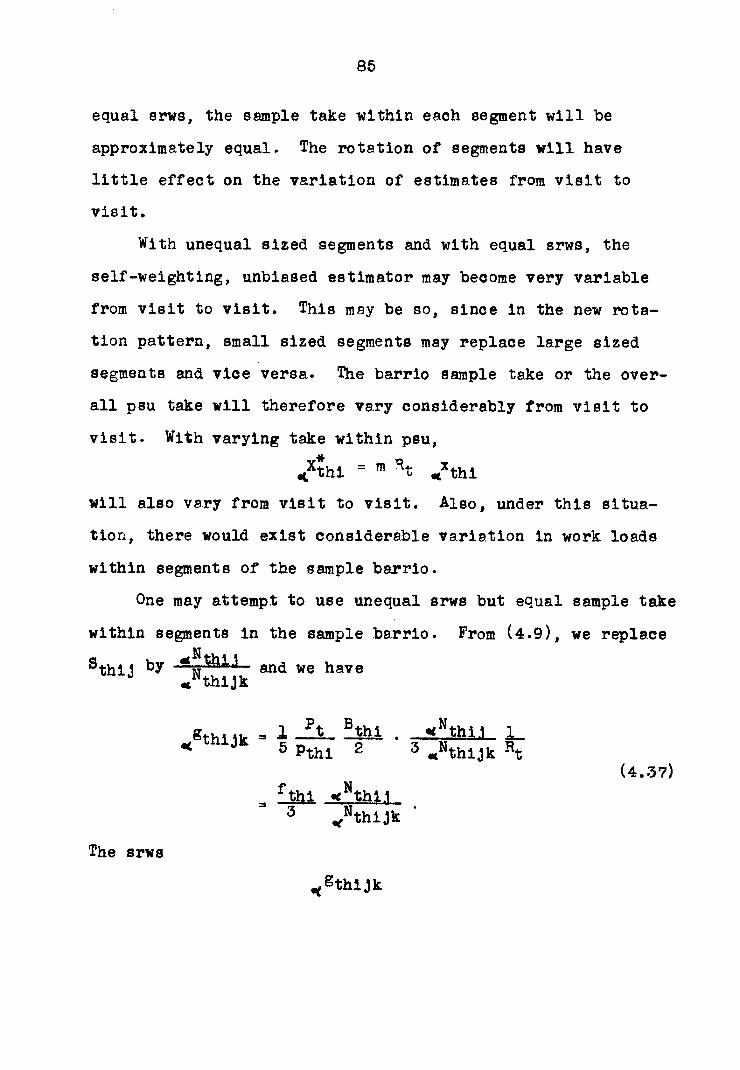
85

equal srws, the sample take within each segment will be

approximately equal. The rotation of segments will have

little effect on the variation of estimates from visit to

visit.

With unequal sized segments and with equal srws, the

self-weighting, unbiased estimator may become very variable

from visit to visit. This may be so, since in the new rota­

tion pattern, small sized segments may replace large sized

segments and vice versa. The barrio sample take or the over­

all psu take will therefore vary considerably from visit to

visit. With varying take within psu,

will also vary from visit to visit. Also, under this situa­

tion, there would exist considerable variation in work loads

within segments of the sample barrio.

One may attempt to use unequal srws but equal sample take

within segments in the sample barrio. From (4.9), we replace

SthiJ by V*1*'1 and we have J * thijk

«"thl.1

*NthiJk (4.37)

fthl <Nthl.1

3 „NthlJk

The srws

<8thljk

86

will now depend on < , and is Inversely proportional to the

size of the segment. Equation (4.20) may be written as fol­

lows :

• & & f £' ^ Ç>*»< • J &

(4.38a)

Substitute "*^1.1 for s in (4.38a), we get *NthiJk thlJ

• sS ? S Ç' •

(4.38b)

From (4.37), we have

^thijk = ^gthijk ^thijk

(4.39)

which implies that ^nthijk in equation (4.38b) is now a

barrio constant and does not depend on k. With (4.39) in

(4.38b), we get

= m R% thi

which is self-weighting but biased.

87

The within barrio bias le

B = effîtiu 2]' *"th1 7*' ytbijkf I 3

k «"thijk 7

- £' — Jîùui £' thijke) (4.41) 3

k «"thijk <nthlJlE Y * j

sthij

Xthlj _ JZ

k thij v «"thijk

where

4^2' -4^ £' /thljkt]= <Xthij (4.42a) 1 3

k «"thijk y " 1

is the thij^ barrio total at visit < ,

and

k

L 53 . (4.42b) sthij -Nthijk

k

Equation (4.42b) is, in general, not equal to ^thij» unless

the Nthijk'8 are all equal euoh that

tte •

or the ratios

88

«fX thi ,1k

<Nthijk

are equal for ail k.

If the segments are drawn with pps, then the bias in

(4.41) disappears. With the new rotation scheme, however, the

drawing of segments with pps is not theoretically feasible.

For a fixed visit , the set of three segments in the sample

is assumed to be a random selection of all possible segments

in a given barrio.

Growth in the counts of hhs in the sa or barrio may be

dispersed or concentrated fl9j. Dispersed growth is one in

which the construction or birth of new hhs and the disappear­

ance or drop-out of old ones, occur eta relatively even rate

in most of the segments in the barrio. This implies that the

rate of growth of each segment, r1, is equal to the rate of

growth of the entire barrio, r, from the ( <-l) visit to the

< visit. Thus for

r1 = r ,

<gthijk = fthl (3>r).<-lNthl.1

(1+r' ) «c-l^thijk

= fthi *-1 thi1 3 <-lN thijk

(4.40)

" *-lgthijk '

In concentrated growth, the rate of growth in a relatively

89

small number of segments Is greater than the rate of growth

of the entire sa. Thus

r' > r

for some segments and

<gthijk < <_igthijk

If

r1 < r ,

then

•<gthljk > <-lgthijk '

In any case, adjustments are made In the central office and

the field procedure is still simplified since the relation­

ships which have to be maintained are,

<nthij = fthi <NthiJ

is the sample take in the thij*'*1 barrio at the

visit,

and

«"thijk = 3hl1

= <gthijk «"thijk

is the sample take in k**1 segment of the thij**1

barrio at the * visit,

where

<gthijk 18 88 defined in (4.37).

For the new segment the field procedure at the visit

90

with unequal srws is as follows:

At the central office, a random start, q, is drawn in the

interval 1 to ^ • This qth hh and every 1 th hh <gthijk <gthijk

thereafter is to be Interviewed. The value of etgthijk 18

obtained from (4.37). A provisional form similar to the one

described in Table 4 is given to the interviewer who lists

the kth sample segment and simultaneously interviews the

indicated hhs in the prescribed form. Additional Instructions

are given in case of non-interview. If an indicated sample

hh Is not interviewed, the cause or causes will be given, and

the next hh to the one indicated is interviewed instead. Re­

fusals will be considered as a different category. This field

procedure is similar to the one instituted for a new segment

with equal srws.

Two aspects are considered in the field procedure for the

matched segments with unequal srws. These are:

a) dispersed growth in sampling area. In this case,

<gthljk = <-lgthijk

and the same srws is used for the •(, visit as in the

previous visit ( <d-l). The interviewer is given a

list of hhs from the ( *C-l) visit wherein are indi­

cated the sample hhs to interview. This list has

been adjusted in the central office for sampling

interval; to take care of drop-outs, non-interviews

91

and other related causes. In addition, the inter­

viewer is provided with a provisional form (Table 6)

which will be used for new hhs (in for first time).

The procedure for new hhs will be similar to hhs in

a new segment. Listing and interviewing are done in

only one operation. Any adjustments are made in the

central office.

b) concentrated growth in sampling area. In this case,

<gthljk < <-lgthljk

which implies that the srws at the (< -l) visit is

greater than srws at the et visit. The interviewer

is provided with a list of hhs from the (k -l) visit

wherein are indicated the list of sample hhs to inter­

view. By and large, these sample hhs are the same as

In the (et-l) visit but the list has been adjusted for

sampling Interval. An adjusted sampling rate is

applied to the list of new hhs such that

adjusted rate x number of new hhs at < visit

= *nd

is the size of sample accruing from the

list of new hhs,

and

*gthljk *Nthijk = < "thijk

= «f nthi j/3

<-ln thijk + *nd

92

where

«(-lnthijk is obtained from the ( *( -l) visit,

*nthijk and *nd sre obtained in advance from

(4.37).

In case,

*gthijk > *-lgthijk '

then similar adjustment procedures as outlined above

for

*gthijk < <-lnthijk

may be used. Note that adjustments are made only in

the second and third visit for any given segment,

since the segment is dropped from the sample after

the third visit.

Listing of the new segment and the matched segments at

the eC visit to record births and deaths of hhs will ade­

quately up-date the sample for the dispersed and concentrated

growths. In general, only new hhs which are included by appli­

cation of the appropriate or adjusted sampling interval within

segments will be added to a particular subsample of hhs from

the previous visit iu -l). Note that ^N^hij and <NthiJk

are available in advance and an accurate knowledge of the

srws

<gthijk

is available prior to the actual field operation. Under this

93

situation any adjustments are easily made in the central

office. Also from the relation

<nthij = fthi <Nthij '

we note that

fthl is a Psu constant

and

et^thlj is the listed number of hhs in the thijth barrio

In general, ^Nthlj increases with * and therefore, ^nthij

and ^ nthljk will also increase with •< , since

v"thijk • •

In summary, the estimation procedures with equal srws

are self-weighting and unbiased and the field procedure is

simple to implement. On the other hand, the estimation pro­

cedures with unequal srws end equal sample take within seg­

ments are biased. The field operation although still simple

is more difficult to Implement than with equal srws. There

is however some control on the variation of estimates from

visit to visit because of equal sample take within segments.

Also with equal take, the work load is equalized within seg­

ments. The extended use of unequal srws will be dictated by

the actual experience gained In the field.

94

V. RATIO ESTIMATION

This chapter will consider en attempt on the control of

the variation in the size of the barrio and its effect on the

precision of estimates of regional and sector totals for the

barrio and on the precision of estimates of the rural area

total and country total.

In addition, ratio estimation will be introduced with

segmentation into the estimation procedures in the urban area.

Since sampling is multi-stage with complete replacement of

the psu sampled at each stage with equal probability, there

is a loss in precision represented by not apnlying the finite

population correction (fpc) ,

1 1 •

which is between 0.93 to 0.95 for Manila, if sampling is with­

out replacement of psu. For the capitals and cities, —IS— / th

0.05, and so the fpc is negligible. In this case, a larger

loss in precision arises through sampling the psu with equal

probability rather than with probability proportional to some

measure of size. The reason for the latter procedure is that

at the initiation of the design for the PSSH urban area, no

measure of size of the precinct (psu) was available.

In view of the above mentioned reasons for unavoidable

losses in precision it appeared desirable to examine methods

of estimation which would improve the precision. To Increase

95

the precision of estimates for the urban area, ratio estima­

tion will be introduced into the design. These techniques

will be extended to the rural area, if found feasible and

applicable.

A, Control of the Variation in the Size of Barrio

This section will consider an initial aspect in the

development of the sample design of the PSSH, prior to the

rotation scheme developed in Chapter IV. Specifically, this

development deals with an attempt to redefine the barrio stage

unit in the barrio sector through control of the variation in

s i z e , N t h i j » t h e n u m b e r o f l i s t e d h h s o f t h e t h i j b a r r i o

in the i**1 municipality of the h**1 stratum in the barrio sec­

tor (t = l). The equalization of size of barrio was realized

through the utilization of an ancillary variable, zthij' the

number of population of the thij^h barrio.

It should be recalled et this point that the sizes of

the strata were made equal through equalization of size of

population of stratum. In addition, the psus were drawn with

pps, the measure of size is again size of population of psu.

One of the most important interests in the design of the

PSSH is the estimation of totals such es the stratum total,

Xth; the sector total, Xt; and the country total, X, of many

characteristics from the sample. Because of this Interest in

the estimation of totals or population aggregates, the control

96

of variation in the size of the ultimate cluster £ 9, Vol. 2,

p. 204^ , for example, the barrio, assumes a very important

role in the efficiency of the design. The berrlo is the

ultimate cluster in the barrio sector of the rural area.

Let us consider the role of the size of the barrio in the

precision of estimates from the barrio sector (t = l) prior

to segmentation. From (3.29), the estimate of the stratum

total, X^, from the 1th psu is

A Xlhl = m Ri xihi

where

m = 5

— 8 50

and

xlhi is the sample total of the 1th psu.

Note that x^^ is the only variable in the estimation pro­

cedure. Any control on the variation of the x-^ will be re-

A p fleeted on the reduction of the variance of X^^ or <T

This sample total depends on the size of sample from each of

the barrios. In fact, from (3.28)

nlhi = flhi S NlhiJ

J

is the sample size from the i*"*1 psu and depends on the psu

constant, flhl> and on the relative sizes, , of the two

sample barrios. One aspect of control in the size of barrio,

^lhij' 18 to equalize their sizes. This equalization will

have a corresponding equalization effect on the n^hl1 s and

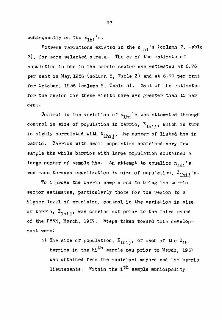
97

consequently on the 1 s.

Extreme variations existed in the n^i's ^co^umn Table

7), for some selected strata. The cv of the estimate of

population in hhs in the barrio sector was estimated at 6.76

per cent in May, 1956 (column 5, Table 3) and at 6.77 per cent

for October, 1956 (column 8, Table 3). Most of the estimates

for the region for these visits have cvs greater than 10 per

cent.

Control in the variation of n^hi'8 was attempted through

control in size of population in barrio, , which in turn

is highly correlated with Njhij' number of listed hhs in

barrio. Barrios with small population contained very few

sample hhs while barrios with large population contained a

large number of sample hhs. An attempt to equalize n^^'s

was made through equalization In size of population, Zihij's*

To improve the barrio sample and to bring the barrio

sector estimates, particularly those for the region to a

higher level of precision, control in the variation in size

of barrio, was carried out prior to the third round

of the PSSH, March, 1957. Steps taken toward this develop­

ment were:

a) The size of population, J ' of each of the B^^

barrios in the hith sample psu prior to March, 1957

was obtained from the municipal mayors and the barrio

lieutenants. Within the 1th sample municipality

98

(psu), the barrios (ssus) were redefined and made

into units of approximately equal size of population.

The first process consisted of combining of small

barrios, with the requirement that the new unit should

have

Zlhl j i 4 50 . ( 5 • 1 )

The second process was to split extremely large

barrios into two or more new units with the same re­

striction as (5.1).

The new unit thus formed is either a group of

barrios, a whole barrio, or a part of a barrio.

Rigorous equalization was attempted in regions with

high cv1 s .

b) Original sample barrios which were untouched remained

in the sample. If two original sample barrios were

combined, another 1 new1 unit was selected at random;

and in case of dissection of a large sample barrio

into two or more 1 new1 units, then a 1 new1 unit is

drawn at random to replace the original big barrio.

c) A new psu constant, (3.28), was computed for the

i*"*1 sample psu. This was brought about by the forma­

tion of a new barrio count, , in the 1th sample

psu. Thus

r ' = 1 LUL, . !m i_ 1 m Plhl blhl Rx

99

where m, , blhl and R^ pre as defined in

(-3.23) .

d) Efforts were made to determine the true boundaries of

the 'new' sample areas. Interviewers were required

to draw sketch maps of the sample areas assigned to

them, indicating areas actually covered, 1 natural'

boundaries, location of hhs, and other pertinent

facts about the 1 new1 sample area. Egoh of these maps

were carefully screened and checked for accuracy.

Completely new listing of hhs was made in each 'new'

sample area.

An illustration of the attempt on the equalization of

population size of barrio through the combining of small

barrios is given in Table 7.

The changes in the number of barrios, ; the psu

constant, and the size of sample within psu, n^hl,

before and after equalization of size of barrio, are illus­

trated in Table 8 for five selected strata.

There is a general Indication of a decrease in variation,

as measured by the range, R, for f-y^ and n^hl. Some general

results of this attempt on equalization are Indicated by the

cv's of various estimates (Table 9). A

The cv of = 14.286 millions of population for March,

1957 was reduced to 2.31 per cent as compared to a cv of 6.77 /X

per cent for = 14.089 millions for the previous round,

100

Table 7. An illustration of the attempt on the equalization of population size of barrio through the combining of smell barrios for two selected sample municipalities5

Stratum V Stratum X 4th sample municipality 5th sample municipality Before After Before After

equalization equalization equalization equalization Barrio Popu- Barrio Popu- Barrio Popu- Barrio Popu-no. lation no. letion no. lstlon no. lation

1 476 2 325 3 230 4 570 5 800 6 1, 080 7 185 8 900 9 680 10 727 11 1, 230 12 650 13 540 14 1, 350 15 680 16 520 17 976 18 760 19 3, 050

1 476 2 555

3 570 4 800 5 1 ,080

6 1 ,085

7 680 8 727 9 1 ,930 10 650 11 540 12 1 ,350 13 680 14 520 15 976 16 760 17 3 ,050

1 876 2 1 ,354 3 3 ,025 4 632 5 445 6 579 7 738 8 689 9 443 10 356 11 428 12 489 13 931 14 391 15 507 16 2 ,792 17 1 ,665 18 938 19 1 ,708 20 500

1 876 2 1,354 3 3,025 4 632

5 1,024

6 738 7 689

8 799

9 917

10 931

11 898

12 2,792 13 1,665 14 938 15 1,708 16 500

aSource: Office of Statistical Coordination and Standards, National Economic Council, Manila, Philippines, 1957.

October, 1956. Similarly, the cv of X, the country estimate,

was decreased from 3.27 per cent in October, 1956 to 2.16

per cent in March, 1957. Most significant were the results

on the reduction of the cv of barrio population estimates for

101

Table 8. Number of barrios, primary sampling unit constant, and number of sample households within primary sampling unit before and after equalization of population size of barrios, for selected strata8

Number of Primary sample house-

Munlci- Number of sampling unit holds within palltv barrios constant primarv

Stratum (psu) Before After Before After Before A|*ter

h 1 Blhi Blhi flhi flhi nlhi nlhi

(1) (2) (3) (4) (5) (6) (7) (8)

5 1 11 9 .038 .031 12 10 2 29 34 .073 .085 36 15 3 17 6 .098 .035 24 13 4 19 17 .066 .059 13 11 5 11 11 b -041 .041 15 18

R =.060 = .054 R=24 =8

10 1 17 8 .177 .083 33 24 2 48 33 .094 .065 10 17 3 1 1 .028 .028 8 13 4 20 18 .053 .048 10 13 5 20 15 .045 .036 28 95

R=.149 = .053 R=25 =12

15 1 24 28 .043 .050 13 15 ? 7 5 .051 .036 6 10 3 21 29 .039 .054 6 19 4 22 40 .036 .066 30 24 5 46 36 .108 .085 44 23

R=.07? =. 049 R=38 =14

20 1 9 6 .049 .033 8 9 2 57 30 .147 .077 21 20 3 67 44 .123 .081 14 13 4 38 21 .082 .046 21 19 5 38 21 .082 .046 12 11

R=.098 =. 048 R=13 =9

2.5 1 34 27 .096 .076 25 19 ? 27 26 .070 .067 33 21 3 13 13 .052 .052 21 21 4 25 18 .074 .053 14 17 5 10 9 .070 .063 13 21

R=.044 = .024 R=20 =4

2Source: Office of Statistical Coordination and Stand­ards, Manila, Philippines, 1957.

bR = maximum - minimum.

102

Table 9. Estimates of barrio population and coefficient of variation of estimates in per cent by region before equalization, October, 1956, and after equalization of size of population of barrio, March, 1957a

October. 1956 March. 1957

Region Estimate

(millions)

Coefficient of variation (per cent)

Estimate (millions)

Coefficient of variation (per cent)

II 1.076 21.92 0.934 10.25

III .593 9.92 .767 6.27

IV 2.505 7.73 9.024 4.74

V 1.871 18.96 1.617 10.43

VI 1.509 17.72 1.431 4.18

VII 2.975 8.07 9.399 4.77

VIII 2.675 11.34 2.876 5.23

IX .839 11.86 1.153 6.53

X .746 19.79 1.085 11.01

Philippines 14.089 6.77 14.286 9.31

^Source: Office of Statistical Coordination and Stand­ards, National Economic Council, Manila, Philippines, 1957.

regions II to X (Table 9). Most of the cv's were reduced

from more than 10 per cent to about 10 per cent or less.

Similar reduction in the cv of the most important character­

istics of the survey was observed.

The equalization of size of population of the barrio will

be a permanent feature of the barrio sector at least for a

103

period of time. The reduction of the cv of estimates for the

region and for the sector is considerable. There is also

some reduction in the cv of the estimate for the rural area

and for the country. This redefinition of the barrio stage

unit did not in any way affect the form of the self weighting

estimation procedures developed in Chapters III and IV. The

simplicity of the self-weighting scheme has been retained in

the design.

B. Ratio Estimation in the Urban Area

As mentioned before, the sample of the PSSH has been

constructed and it consists, .apart from minor substitutions,

of the same panel of primaries, secondaries and tertiaries.

Thus, in the urban area, improvement of the efficiency of

the design may be accomplished through a change to a ratio

estimator. As auxiliary variable, we will use the list or

count of registered voter ( «Z^hl^ which is available by

precinct from the Philippine Electoral Commission. National

election is held every two years ; the latest was held on

November 10, 1959. This auxiliary variable is up-dated every

two years. Biased and unbiased ratio estimators will be dis­

cussed for possible incorporation into the estimation pro­

cedures in the urban area.

104

1. Biased ratio estimation

We have from the 1th psu of the th^ stratum an inde-

pendent unbiased estimate, ^thi> the stratum total,

•cXth* There are five such psus drawn sequentially and thus

there are five such independent estimates, and the mean of

these estimates, is also an unbiased estimate of < .

Each ^X.^^ is considered as an independent observation from

an infinite population of ^thi at the * visit. With this

consideration, standard techniques on ratio estimation for

simple random sampling can be utilized. Specifically, the

ratio of means estimate jllj will be introduced into the esti-A.

mation procedures. The regular unbiased estimate, X or •C till

*** 1"Vi zthi of the stratum total from the 1 psu, will take dif­

ferent forms depending upon the nature of the design employed

for the secondary and tertiary stages.

Consider first the estimation of the stratum total,

^Xth, will be for population in hhs and occupation of head

of hh. These characteristics are obtained in the first phase

or listing operation of the segments in a rotation group or

of the whole precinct if there is no segmentation. Three

forms of ratio estimation will be discussed; one of which is

applicable to any given stratum.

a) complete ratio estimation. The segments in precincts

are known, recognizable and identical for both

electoral list and survey list. Street names or city

105

blocks may be used to Identify segments in precincts

with electoral list for the precinct. Bias should be

eliminated in the listing within segments.

Consider as estimate of ^th»

Jto • Jth ,Zth (5.9)

•c thij

and

Ah * ir Mth 5m

i J

<XthiJ is the listed segment total at the <

visit

et^thij the corresponding electoral list total

for the segment at the «C visit ( closest

electoral year)

^Z-th the electoral list total for the th^*1

stratum at the < visit.

Equation (5.3) is too cumbersome to compute. With the

use of self weighting scheme given in (4.31), (4.32)

and (4.33), (5.2) becomes,

% ** Y * th 7 /_ .X

m Ath = etzth 15.4)

<zth

where

V 3 ml j

*4h - 22 53* e , (6.5)

106

(5.6) * thij - thlj « thij

ethij = 5r Mth s; • l5-7)

Thus, the numerator in (5.3) is equal to

*Xth = m E2' »", £' 4hij

1 j (5.8)

V} X"1' #* D *# - Rt Zv 2u xthij = t <xth •

i J K

The same result is obtained for the denominator. The

Rf. cancels and we have the result given in equation

(5.4).

The bias in is obtained from the relation,

E (<Xth ] = KXth " Cov K th- * Zth (5.9)

and the bias is therefore equal to

- °ov( qth, (5.10)

where A y*#

~ _ K^th wqth -

«zth

#» «%th

** zth

and

V* t** Xth or is as defined in (5.8)

The upper limit of this bias is

107

I Blssl - yà 9th CV< -t2»!1 (5.11)

where d~

ov'.zthi> oc th

?** p * thi " m Ht «^"thl

** Z^4 ,

^ *

^2 o n** -txthi

Ah thl

- 2 }

(5.1?)

(5.13)

(5.14?)

or

y** = — ^ 0** oC th in ot thl * %th

(5.14b)

and

Q oC^th = «%th

An approximate estimate of the approximate vari­

ance formula given in equation (5.14s) is

2 % = m m - 1 «t tn

2-y oc thl + a-th ZL

2 ~2 X-1'

' V * thl

- 8 Jth z ) •£** ç** o< thl ^ thl

(5.15)

which simplifies for computational purposes Into

108

S~iHf- = <t ? M ? - ' * P » »

«xth " m - 1 ~ o<fxthl + «*ath }__J *.zthi 1 i

# v—;) 4H* •>!••«• ~ *qth Z_y ocXthi *zthi

where

(5.16)

od Xthi en^ * thl Rre as defined In (5.1-3).

A gain in reliability of ^ to that of ^ X^.^, the

x-only estimate, is achieved if y\ ,

(°$»* S»e \ 1 Cy^ °cZthl ) (5.17) / - thl' « thl ' ? ov(

w h e r e / ° i s t h e c o r r e l a t i o n b e t w e e n X * * / ot

Xthi> 7w1f -Lb Uric CO I x C_Lc: UJ.UH be UWctîIl . +^4

*z thl " x n i

and ^ thi ' CV^ <*. Zthi ?nd CV^ *Xthi^ ?re ps defined

in (5.1?). Relation (5.17) is derived by making the

last two terms in (5.14a) less than zero, i.e.,

*4 4%, -? Ah %i, <0

where

""th = '

ratio estimation in the primary stage. In this case,

the segments in precinct are known and recognizable

for the survey only. Available are segment totals,

ot Xthi j ( J = 1,9,3) and the precinct (psu) totals,

cl Zthi ( 1 = 1,9, . . ., Mth) . The ratio estimator has

the form

109

F )

^ 22' Lv x.

" 3 ' "-i .Zth (,i.)

^ £'

i

which simplifies into

z:' x-«c thi Xth - —— .Ah (5-Mb)

Z7 ec Zthi ^ un y-,) _ <

i

where

^X|hi is an unbiased estimate of the 1th psu

total, ^%thl -

The ratio in (5.18a) or (5.18b) may be expressed in

terms of 1 sample1 totals. From eauetion (5.8) the

numerator is eoual to

*** R ** ecxth = Rt «^Xth

and the denominator is equal to

* 5 oL Uli u <<

zth = Rt ^z-th (5.19)

where

* V75 * «<zth = £—> ot

zthi » 1

zthi = fth <vZthi

and

fth = m *th Rf '

Thus, we ^ay write (5.18b) as

110

A th = ^-th th

where

> • a The biss in is

- Cov( ^qth, eCzth^

and the upper limit of the bias in (5.?l) is

(5.90)

( 5.21)

|Blss| ± "j,. CV( kth

where

^1% = m

r

<«•# +

*Xthi Ql f~3*

oC th oL thi

(5.22)

- 2 th 9».v JÎm > • (5.93)

^ thi R tt

t ^2* thl ;

,^th = <^.Xth

^ Zth

(5.24)

and

cv( Ai> - Sf

The covariance will probably be smaller than in case

a) and hence the variance of the ratio estimator

larger. The approximate estimate of the variance in

equation (5.23) is

Ill

2

eCXth & X

) ? r* 'thl

* v-> - ? thZv

*** *</thl "thl (5.25a)

where

and

Is as defined In (5.20),

xthl ls 88 defined In (5.5)

^zthl 85 defined in (5.19)

A gain in precision of the ratio estimator, •a Y**

, xth'

to that of the x-only estimate, ,Xth is obtained If

A.. - \ i cv(.4hi)

^.%'^hl / GV(^)

(5.25b)

c) no segmentation. The precinct is completely listed

by the survey. We have available at the precinct or

psu level, the psu total, ^^thi = 1, °,3,4,5) and

the psu electoral count ^Z-thi (1 = 1>9, • • • , ^th^ '

Let the estimator be 3, x*

eC^th ,4th 'th (5.26)

where

,4th =

Mth

i m ocXthi

*Zthi

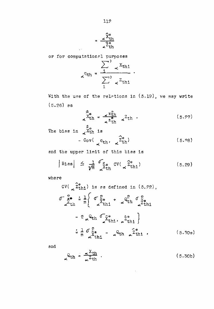
IIP

X* _ th

2* * th

or for computation?! purposes

E' x»! i "c

,qth =

i

With the use of the relptions in (5.19), we may write

(5.26) as

A Xth = - 2*h -dZth * (5.27)

<*. th

The bias in ^X^h is

- 9th' ^%th) (5-98) Q+->i »

end the upper limit of this bias is

|B1SSI - V5 5ïhCV(^thl> (5.89)

where

CV(^Z*hi) is es defined in (5.22),

rh1 H 'Ai+

-2^h<rÂi. Ai}

° » ^Jthi " Ah -2»1 '

and

Q ' ^ 'th

°cXth

(5.30a)

^th = z~Z • (5.30b)

113

To estimate the variance in equation (5.30a), we use

SSW = m Ri it

i eC

xthi * eeqth zthi /th m - 1

" 2 -th Z xthi ./thl J (5.31)

where

q^ is as defined in (5.Pô) «<

A gain in reliability of ^th to ^^th is achieved if

-Av

rxthi snd zthi sre as defined in (5.19).

X* Z* ) 1 CV( ^^HI) , (5.32) «( thl' thl ' " CV( *X*hl)

The forms of the formulae for the estimator, bias, upper

limit of the bias, approximate variance and its estimate are

similar in the three forms of ratio estimator. The difference

lies in the estimation procedure accruing from the 1^ number­

ed psu and the sample mean or total of the five psu estimates.

These estimates were then reduced to their corresponding self-

weighting form for easy comparison with the regular unbiased

self-weighting estimates developed in Chapters III and IV.

A 1 separate ratio estimate1 for the t^ sector total,

, is obtained by summing through h(= 1,2, ..., L%), the

stratum estimates given in (5.?), (5.18a) and (5.26) and

similarly for the variance of estimate and estimate of vari­

ance. Thus, the separate ratio of means estimate of ^X% at

114

the oi visit assuming no segmentation in ell precincts is

obtained from (5.25) and the estimate is given by

Lt 59

<AS Y* V Y* XtR = I—/ * th

h

Lt

= ZZ 9th %th - (5-33) eC h

If (5.2), (5.18a), and (5.26) are used with different number

of strata, ^Qth ln (5. 53) is replaced by ^th (5.2) or by

th ( 5.20) as the case may be. The auxilliary variable,

e^Zth, the count of registered voters in the electoral list

in the th^*1 stratum at the -x. visit, is available at no cost. A*

The approximate variance formula of ^X-t is derived from

(5.30a) and its estimate is obtained from (5.3l). Thus

= (5.34)

and its estimate is Lt

2 v •/ 2 S*.» = y s%* . (5.35) A

With different forms of the ratio estimate in different

strata, the approximate variances of the strata are added to

obtain the variance of the separate ratio estimate. An esti­

mate of each of the variances is computed in a similar manner.

A 1 separate ratio estimate1 for the urban area (t = 3,4)

115

is obtained in a similar manner. The sum on h will be through

(Lg + L^) or the total number of strata in the two sectors.

A 1 combined ratio of means estimate1 of the t^*1 sector

total, ., will now be derived. An unbiased estimate of

from the 1^^ psu is

 • Û h=l

Jtb

X. tphl * h=l

t«hi 1 h=l

=3 at( *x"i+ +

A1 r (5.36)

= m R+( . * ti)

where

,xti ^*t%i + *x*2i + ^xtci

Lç is the number of strata under complete ratio

estimation (5.9),

L^ is the number of strata under ratio estimation in

the primary stage (5.18),

L.J. is the number of strata under no segmentation (5.96),

Lta + Ltb + Ltc = Lt> (t = 3,4)

and the other symbols are as defined in (5.2), (5.18a) or

( 5.18b), and ( 5.26) . The components in ^ xj.^ are corre­

sponding numerators in the ratio in (5.2), (5.18a) or (5.18b)

and (5.26) but only from the i^ psu. Similarly, the de­

nominators will provide an unbiased estimate of the sector

count, Z^, from the 1^ psu. Let the i^*1 psu estimate of

116

'Zt be

*Zti

Lt, Jtb Lt,

= Z 1 + z; + Z j; h=l h=l h=l

•< uc hi

= m R t e<Zti

wnere

n »czti -cZtal + <zthi + »<_ztcl

(5.37)

'a-1- <*- "fc-1- ®v uc

end the other symbols ^re as defined in (5.36).

The combined ratio of means estimate of from

mean or total of the five t>su is

*Xt= ' <Qt y

where

0+ = •c*t

the

(5.38)

& - i

)

* x t l

= R t ^%t

(5.39)

and

~ i rJ t m Z—y »cZtl

= R t x.Zt

(5.40)

cL Zt is the count of registered voters in the electoral

list of the t^h sector.

Again, Zt is available for all t (3.4) and at no cost to

117

the survey.

The ciPS in is

i, - Cov( ^qt, Zt)

and the upper limit of this bips is

lBlssl

(5.41)

(5.4?)

where

°T< J l O - -% c C U

Xt, = 1J cr S

m ^Xti

p <r? <r. 7" ~ 9 u X* 7 <*/ti * ti> ti

and

^ " "Â

The estimate of the variance in (5.4-3) is

.9 m

m -W x t i + oC ti o<_ ««i: up

*cZti

(5.4-3)

- 2 c X. h »cxti oczti

(5.44)

where the symbols are as defined in (5.37), (5.38), (5.39)

and ( 5 .40) . S3

A pain in precision is achieved with the use of . X+-^ uc

(5.38) over ^X^. (5.39) if

*m. > a

i ov(-zti'

cv< x.4i)

(5.45)

118

We can obtain an urban estimate ( t = -3 and t = 4) by

combining for t = 3 and t = 4 to give an unbiased estl-

"•'II mate of ^Xg + ^X^ and so with ^for t = 3 and t = 4 to

give an unbiased estimate of *,Zg + ^ Z^. Thus our combined

ratio estimator of ^X3 + ^X^ is

f J.3 + **4 , „ , *•(-3+4)0 = —^ ^ ( »Z-3 + -Z4)

œZ3 + o6Z4

Z' Ji - -t— Z zt (5.46)

£ Z," * Pt "t

where

Z ' - Z -O

t=3

th For example, the i psu estimate of ^X3 + ^X4 is

r Xti " m Rt^ «<x3i + ocX4i^ (5.47)

t

and the 1th psu estimate of ^ Z3 + ^Z4 is

53 «cZti = m Rt^ =cz3i + »<z4i^ (5.48)

t

where the symbols are as defined in (5.36) and (5.37). The

bias, upper limit of bias, the approximate variance formula

and its estimate and the relation to obtain a gain in pre­

cision are similar in form to (5.4l), (5.4?;, (5.43), (5.44)

and (5.45), respectively.

119

Three forms will be derived for the case in which a

general characteristic, eCxthi1k» is observed in the sample

hh. The three forms of ratio estimator will depend on the

stage in which the Z variable is observed or is made avail­

able . The three forms are as follows :

a) estimation from the sample hh stage. The auxilliary

variable, ^thi jk> observed on a sample hh basis.

This may be obtained by adding a question in the

demographic block or section of the questionnaire

which is used in the second phase of the field work.

It should be pointed out that this technique is too

difficult in practice. In this case, the ratio of

means estimate will involve the ratio of two regular

unbiased estimates ( 4.96 ). The form of the estimate

for the stratum total, X^, is

ag^th = ^%th (5.49)

where

n - * Xth

"g9th " À and

„Xth, are as defined in (4.56) .

b) estimation from the sample segment or secondary stage.

The count of registered voters, ^ thij > available

at the segment or secondary stage while %thijk ls

observed at the hh level. In this case, the form of

120

the estimator is

*gXto - Ah (5.50)

where ,X 3** - * th

<*g -th A** » ®c th

e^^th is as defined in (4.2.6)

and

is as defined in (5.8).

c) estimation from the sample precinct or primary stage.

In this case, the count of registered voters, ^%thi;

is available at the precinct level and is

still observed at the hh level. The estimator is of

the form

,g% = <5-51'

where ^

5** _ *Xth eig "th

et^th

Xth is as defined in (4.26) ,

and

xZth es defined in (5•19).

The bias, upper limit of the bias, approximate variance

formula end its estimate and the pain in reliability of the A

ratio estimator to that of ^X^, the x only estimator have

the same form as described in the case of estimation for

listed population and will not be given in detail. Similar

forms as given in (5.3-3), (5.34) and (5.35) are derived for

191

the separate ratio estimates of a sector totsi or the rursl

area total. The combined ratio of means estimste is

=tgXt = dga-t (5.59)

where

~ X •

= Rt ,

Lts Ltb Lt0 -V"

A = XJ ^zth + S zth + S Z

h h h

y

snd

LtP + Ltb + Ltc = Lt •

The bias, vsrisnce snd its estimste, and the relation to A

achieve a gain in precision to thst of sre easily derived

snd sre of slmilsr form to thst obtained for s stratum esti­

mate .

2. Unbiased rstio estimation

If the size of sample pairs, say, ( xthi> ocZthi' drawn

from each of the L% strsta in the t^^ sector is small (m = 5),

then the bias in the ratio of means estimate (5.9, 5.18, 5.96,

5.49, 5.50, 5.51) of the stratum totsl, X%h, may have the

same sign, and the bias in the separate ratio estimate (5.33)

of the sector totsl, X^, will be approximately Lt times that

for s single stratum totsl while the standard deviation of

the sector estimate is multiplied by l/L^ ^9, p. 130; sj . Note

122

that the component estimates prising from each stratum may

have different forms. In this situation, the order of mag­

nitude of the mean square error of estimate of the sector p

total is L|; while, if the estimate of each stratum total is

unbiased, the order of magnitude is only ["ôj. The use of

unbiased ratio estimators is of some advantage under such

circumstances.

Hartley and Ross [*12 J gave exact expressions for the

bias in the ratio of means £llj and mean of ratios , p.

124J. From these expressions, an unbiased ratio estimator

is derived. In subsequent discussions on unbiased ratio

estimation, it will be assumed for simplicity and clarity,

that the precinct or psu is completely listed by the survey

(ë.26) and that there is no segmentation. In addition,

empirical results given in the next section (Section C) will

utilize the forms which will be derived under the above

assumption.

The unbiased ratio estimate of the stratum total, ,

is defined as

<Xth = etrth *Zth + m - l ( »cXth - ^th „^tV (5.53)

where

oi rth m e>c rthi

^rthi -«i thi

123

J'thi» ^%h snd ^'ih sre ss defined In (5.19),

(5.21), and (5.26),

^th is the th^h stratum count of the auxilliary

variable,

and

m = 5.

Note that the first term in (5.53) is the mean of ratio esti­

mate £ , p. 124 j of ^xth- Let

^%th = ^th ^th ' (5'54)

The bias in (5.54) is

- Cov( *rthl. *Zthi> <6-55)

which is estimated unbiasedly by the expression

" m - i ZZ (*.rthi - ^th^ *%thi ~ Âh^

( 5.56)

where the symbols are as defined in (5.53). The expression

in (5.56) is added to (5.54) with a positive sign to derive

the unbiased ratio estimator, (5.53).

The exact variance formula of ^is derived [s] by

essentially utilizing the moments of bivariate sample cumu­

lants. A simpler form of this variance is

= m Ai ' •> -'*hl

2

(5.57)

124

which becomes for large m.

^th ° ™ ~ -<Rth *zïhl <s-68e)

or

( 5.58b) *4h * ™ iJtti+ Âi_ ? -Hth ^ïhi, Jîhl

where

„iRth = E( ^rthl) .

The variance of in (5.58b) may be compared with the

approximate variance formula (5.30) of the biased ratio of

means estimate (5.26). Equation (5.30) is appropriate for

large m and is derivable by a Taylor expansion with exact

remainder term £llj. This form is considered as standard in

literature. Thus, the difference between (5.30) and (5.58b)

is

' "Ah ' ™f( ' ~R?h) ""Ai

"s 5thi, ïhi( >h ' } (5-59'

- ( <<Rth " ^th^ |

where

,X, - th 2

oi, ^ ' -Zth

^th = E( oCrthi)

125

Bth - -^1 7*

OL^thl

pczthl

is the regression coefficient of ^thi on ^thi.

ot th is more efficient then if

( oc^th ~ x.^th)" ) ( ^Rth ~ oc^th^

I.e., the regression coefficient, is closer to ^^th

then to ^Q%h. When ^Rth = ^^th or ^<_Bth ls halfway be-

tween ^^tii anâ- c<^th> when ^X^ is unbiased, then | *A

oJ th snd th pre equally efficient. Experience of Goodman

and Hartley |V] seems to indicate that for th >

oc th ls often found closer to Q h than to R h and in this

case is more efficient than The extent of the

bias in ^X^.^ must be taken into consideration in making a

decision on the estimator to use.

The appropriate estimate of variance given in (5.58) is

9 <*. th 5 L ' ml = 1L, + Jth =|*hl _ 9 ^ thi

r -f-V Sy# 71 * *cthi' «c thi

(5.60)

where

x^th

V-7) = ^ y m Z—'

i **thi »

2 sc* /thi m 2 ' < Ai

and

126

so* = r ec thi > «<. thi " ~ 1

Z ( Xthl

Nieto M

has shown that

(1 < £* et. thl' <*. thi

) m(m - l)

( m^ - m + 1)P +1

' r> ?* x. thi, ei thi

Cth ( 5.61)

where

'th = {^il 2 ( X* T, z" { <<Xth - ^^th «< th'

estimates with a slight overestimation

2 - o

1 S. 'Â, (1 ^

^rthi> ac^thi

which is the second term in the variance expression for ^

(5.57). In fact, an upper limit estimate of this second term 5

is obtained if in (5.6l), /° is made eaual to one / r, 7* J <*. thi > thi

which implies a maximum value for (l + f ) Thus J 2* '

ythi, Zthl

to estimate completely (5.57), we use the sum of (5.60) and

;•>> = 1, (5.61) with /°

J ,rthi >

6?

* thi, "thi

1 \ 9 ,x;h -mi =5* x:_ + ^th

m

* thi

2

ss* - 2 r^t_ ?» oc thi »C 011 thi > ^ thi

m - 1

oL

(m^ - m + l) + 1 • rth oi"th

Z* )? .

(5.6?)

197

To indicate the magnitude of the second term In (5.6?) for

m = 5,

m V S = 0.14? .

. M ~ ^ J (m^ - m + l) + 1

A separate unbiased ratio estimator of the sector total

or a regional total may be derived with the use of (5.5-3).

With independent sampling in each stratum, the separate un­

biased ratio estimate of the tth sector total, is

Lt .1

«As " »cXth h

Lt

= 23 (e6 rth ^,Zth + F~T~1 ( <Xth " ^th o^tV J h ( 5.63)

where

Lt is the total number of strata in the t^*1 sector

(t = 3,4), or the number of strata in a region if

the estimate is for a regional total.

The variance of is obtained from (5.57) and is given by

• 2

Lt-

ot ts ^ »CXth h

L t - E C i <r s

= 2-,|m Jtthi ~ Ah thi * ml m - 1)

{ 1 + f [ 2 . < 6 ' 6 4 )

ot thi ' u thi J

128

Estimate of this variance is given by

Lt .2 -2

h

where

= V sr. i (5.65) «T ts 7~ *Ath sx.

s^i is defined in (5.60), th

or by

?x' - È ?x' /ts f-s /th

where

? % is defined in (5.6?). oC th

The 1 combined unbiased ratio estimator' of the t^ sector

total at the =<_ visit, ( t = 3,4), is given by

«<xtc = ^t + rri ( - *rt *tzt) (5.66)

where

- rt - i 23' i

r. . Jîi - " " J t i •

^t x* x* * t i = 2 _v /thi »

h

X = m S' «Xt'i

199

oL Xthi defined In (5.96),

^Zt Is the t^^ sector count of the auxiliary variable,

and

m = 5.

and are as defined for the X's. The vari­

ance of is similar in form to that given in (5.57) or

(5.58). The components therein are however in terms of sector

totals, sector ratio and sector correlation. The exact vari­

ance is

rx' -i *. to m [""jïi ' A - ? «cRt «&, fa |

m (5.66)

+ r-ÏT(l+/^ . > ">ti "jh <X_ tl ' at. U1

which simplifies, for large m, into

<rf;i = - r<3"|* + R^ <r|# - p Rt <f~£# ^ X ( 5.67) *Xti * ^ti ^ ^Xti, *zti I d%tc %

where

Rt = E( *?tl)

To estimate the expression in (5.67), we have

'X = m f :%1 + A *K - y?1, j>u } <5.68)

where

"lxti ~ m s?# = —^ Y, ( *X*i -

i

? H E' < A -Tt i= •

130

sx* ît, - ^3 Z' ( Jti - X)( Jti - /t1 -ti' ot ti

X

and

»Crt = m 51 * 1

An estimate of (5.66) is

£ 2 . _ l f _ 2 2 ? / t = - m l T ^ J t i - s = x » v J « t l ]

f i2

m m - 1

A4t . 9

p—2-t^- ( A - /t <?V (m*- - m + l) + 1

(5.69)

where the symbols are as defined in (5.68).

G. Empirical Results

Data on the number of registered voters, ^Zthl, by

sample precinct were obtained from the Philippine Electoral

Commission for seven randomly selected strata (h = 1,7,14,

20,21,30,32) in urban Xanlls (t =4). The subscript < in

eC^thi refers to the November 1957 election. Data on the

number of listed population in sample precinct, ^^thi » snd

the number of interviewed population In sample hhs in sample

precinct, ^x-thi' f°r the same seven strata were obtained

from OSCAS, NEC. The oi subscript in oc^thi sn<3- aCxthi refers

to the October 1957 visit of the PS3H. Registration of voters

for the November 1957 election was held at about the same time

131

as the interview week of the October 195? round.

«cXthi> c^xthl and <<Zthi sre Piven in columns 5, 6 and

7 of Tgble 10, respectively. An estimate of the th^ stratum

total, or is computed from each of the five

numbered psus (precincts) in a given stratum, using the

appropriate ^^thi» *<xthi ' or *.Zthi1 These estimates -"re

given in columns 8, 9 and 10 of Table 10, where

C# o * ot thi = m Rt ot

xthi '

and

Jthl = Rt .cHhi

are as defined in (5.?6) , A

*Xthi = m Rt *xthi

is as defined in (4.?6) ,

m = 5 ,

and

= 400 ( t = 4 )

The number of psus, %%%, in the th1'*1 stratum and the stratum

constant, ft^, are given in columns 2 and 3, respectively,

of Table 10.

An analysis of covariance of listed population estimate, A # yt

ocXthi> on registered voters estimate, ^ zthi> lR prepared and

the results are shown in Table 11. A pooled estimate of the

correlation between ^xthl sn<3 e<.zthi computed with the

help of the between primary within strata mean sauares. The

pooled sample correlation is

Table 10. Sample of strata, in urban Manila for estimating p-ain in reliability of biased and. unbiased, ratio estimators

Sample M.xthi *xthl x.zthi Stratum precinct (thou- (thou- (thou-(h; lxth fth «< thi **thi <* thi sands) sands) sands)

(1) (2) (3) (4) ( 5) (6) (7) (8) (9) ( 10)

1 79 0.036 1 549 15 997 39.5 30.0 16.3 2 1127 59 180 81.1 104 .0 13.0 3 937 33 151 67.5 66 .0 10.9 4 759 49 176 54 .6 84.0 19.7 5 899 19 180 59.7 38.0 13.0

Total 309.4 399.0 65.9

7 68 0.034 1 543 96 143 36.9 59.0 9.7 2 699 °4 275 47.5 48.0 18.7 3 492 25 949 33. 5 50.0 16.5 4 531 96 951 36.1 59.0 17.1 5 1352 60 993 91.9 190.0 15. °

Total 245.9 399.0 77.9

14 80 0.040 1 1865 69 948 149 .9 138.0 19.8 ? 1520 56 179 191.6 119.0 14.3 3 350 10 170 98.0 90.0 13.6 4 1138 35 309 91.0 70.0 94.7 5 9996 92 341 17P .1 184.0 97.3

Total 567.9 594.0 99.7

2.0 80 0.040 1 577 92 pop 46.9 44.0 18.2 2 916 30 930 73 .3 60.0 18.4 3 870 40 979 69.6 80.0 99.3 4 1405 57 991 119.4 114.0 93.3 5 1649 69 309 131.9 138 .0 94.7

Total 433.4 436.0 106.9

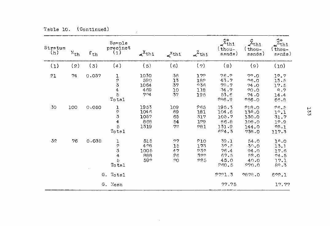
T able 10. (Continued)

Stratum (h) Mth fth

Sample precinct (i) -cXthi <Xthi <*.Zthi

* thi (thou­sands )

Âhl (thou­sands )

3" «/thi (thou­sands )

(1) (2) (3) (4) ( 5) (6) (7) (8) (9) (10)

21 74 0.037 1 1030 36 172 76.? 7° .0 19.7 p 590 13 182 43 .7 °6.0 13.5 3 1064 37 *36 78.7 74 .0 17. 5 4 469 10 118 34.7 20.0 8.7 5 7°4 37 195 53.6 74 .0 14.4

Total 286.9 P66.0 66.8

30 100 0.050 1 19 53 109 265 195.3 218.0 26.5 P 1046 69 181 104 .6 138.0 l°.l 3 1057 65 317 105.7 130.0 31.7 4 868 54 129 86.8 108.0 12.9 5 1319 72 281 131.9 144.0 P8.1

Total 624.3 738 .0 117.3

33 76 0 .038 1 515 27 210 39.1 54.0 1S.0 ? 4P8 15 173 3P . 5 3O.0 13.1 3 1005 47 P.3 9 76.4 94 .0 17.6 4 888 26 3 PC 67.5 52 .0 P4.5 5 59° ° 0 225 45.0 40.0 17.1

To tal 260.5 P70.0 88.3

G . Total 9721.3 P878.0 6*2.1

G. Mean 77.75 17.77

Table 11. Analysis voters,

of covsrisnce

J- thi

of listed population, o L X* thi , on registered

Source of

variation

Degrees of

freedom

Sum of squares (thousands)

-^ean ( thou

souare sands)

Source of

variation

Degrees of

freedom X? zp XZ X? Z2 XZ

(1) (2) (3) (4) (5) (6) ( 7) (8)

Between strata 6 28,851.14 470.37 3,082.67 4, 808 . 52 78.39 513.78

Within strata 28 31,684.19 594 . 50 2,140.29 1, 131. 58 91.03 76.44

Total 34 60,535.33 1,064.87 5,292.96

135

_ 76.44 r 3* -2*

,xthi> eCZthi 1/1131.58 V?I7p3

76.44 " (33.64)(4.61)

= 0.4929 .

An estimate of the coefficient of variation (CV) for an -A

individual estimate, ^^thi or <*Zthi> *s obtained from Tables

10 and 11. The estimated CV1s are

°"v( A' .

and

= 0.4327 ,

- ifti

= 0.2594

A gain in reliability is achieved in the use of ^

(5.26) to that of the x only estimate, ^ %th'

icv( /zïhi» Y,r 7 ^ y 9 . .

oc thi ' a thi / ^ CV( X+V,J eC thi

This relation is estimated by

r 2* = 0.4929 * thi ' «c thi

1 *^h1^ = 0.9998

2 °v< Xhi>

or

136

i c~v( X hi' tV* "y # y 9 «X A.-j. .

/thi' /thi ' - cvt ^X^hi)

By and large, we expect a gain In precision in the use of

A# oC^th' ratio of means estimator as compared to the

x-only estimator.

Similarly, an analysis of covariance of the interviewed

population estimate, ^xthi' on the registered voters esti-

mate, ^zthi' is computed and the results are summarized in

Table 12.

From Table 12, we have

r $ > 0.4567. ot thi > ^thi

From Tables 10 and 12, we obtain

1 SliJk1> . 0.9774

2 cv< JthO

Finally, we have the relation A CV( "z* J

r >v.. si K thi

<k XthV /thi > ? CV( xthl )

This result indicates that, on the average, there is a gain

in reliability in the use of ^g^th (5.51), as compared to

the regular unbiased estimate, X^-

The mean of ratios ( r^) , ratio of means ( and

estimate of the variance of _X^ and pn^- their covarl-

ances are computed for each of the seven strata. The results

Table IS. Analysis of covariance^of Interviewed population, ^xthl« on

registered voters, ^ thi

Source Degrees 0f 5f bum of sauares ^ean square

variation freedom X- Z - XZ X? Z XZ

Between strata 5 35,414.18 470.37 3,466.93 5,909.36 78.39 577.8?

Within strata 28 41,375.^0 594.50 2,056.68 1,477.68 91.93 73.45

Total 34 76,789.18 1,064.87 5, 523.61

1-38

are summarized in Table 13.

For h = 1 (Table 10),

r = If 39.5 , 81.1 , 67.5 54.6 . 59.71 th 51 16.3 13.0 10.9 19.7 13.0 J

= 4.75 ,

= 4.59 ,

8^* = ôif 16.3S + 13.0? + 10.9P + 19.7? + 13.0? - 9 J,th 20 [ 5

= 0.76

and so on. From Table 13, the estimated variances of the

Table 13. Mean varia

of ratios, ratio of m nee for each stratum

eans and esti -'ate of

Stratum (h) e<.rth ocqth

2 s ç*

/ * th (thousands ;

? S A*

/ 06 th . (thousands)

8 , * th' = th (thousands)

(1) (?.) (3) (4) (5) (6)

1 4.75 4.59 47.49 0.76 -4.il

7 3.31 3.18 119.78 9. 37 0.82

14 5.66 5.70 666.49 7.44 42.98

90 3.96 4.05 240.79 1.73 17.62

91 4.99 4.99 76.93 9.09 8.29

30 5.58 5.39 361.77 11.94 29.97

32 9.93 2.95 71.56 3.53 10.44

139

regular unbiased estimate (the x-only estimate), ^X^h (5.19);

the biased ratio of means estimate, ^^th (5.95); pnd the un­

biased ratio estimate, c<: xth (5.53) and the relptive effi­

ciencies of and ^X^ to ^X^ are obtained for each

stratum. The results are summarized in T^ble 14. For clar-

i t y a n d e a s y r e f e r e n c e , t h e e s t i m . p t e d v a r i a n c e s o f ^ ,

.jj, |

*xth pnd a%th pre ^lven telow. For

2 s-w is as given in column 4, Table 13, and is d^th 2

computed similar to s5'M above. a* * th

For X (5.26, 5.3l), «< th

9 2 ? + a" s-* - o a

/th /th ^"th /th /th J*th, /th

For ^xth (5.53, 5.60),

;L ' :L * - rL &, -? %, a •

ivote that the gain (h = 14,90,21,3°) or loss (h = 1,7,3?) in

-ÎÎ- j «jj, estimated efficiency of ^xth Pnd ^xth to ^^th pre approxi­

mately eoual for all h. These results are to be expected

since ^th approximately equal to oCcxyï for the seven

^ 1 strata. From these estimates, we say that ^X^ and ^^h

are equally efficient.

If the seven strata are considered as a sector, then five

different estimates of the sector total, ^X^, may be com­

pared, namely:

140

Table 14. The

and

estimated variances of

the relative efficiencies of

-a# i <£Xth ^xth Xth *</th

to a%th for e?ch stratum

Stratum (h) Estimator

Estimated variance

(thousands)

Relative3

efficiency (per cent)

(1) (2) (3) (4)

1 y*

X* x th

47.49

101.93 46.91

A 103,69 45.80

7 Â Â

119.78

138.52 86.47

4%th 140.33 85.36

14 x* ot th 666.49

*Ath 418.25 159.35

A 417.00 159.83

20 240.79 — —

x^ th 126.44 190.44

<%lh 128.37 187.57

21 X* /th

X* a . t h

76.23

42.27 180.34

y1 ^th 42. 97 180.34

BThe estim ?ted variance of ^Xth is used as numerator-

141

Table 14. (Continued)

Stratum (h) Estimator

Estimated variance

(thousands)

Relative efficiency (per cent)

(1) (?) (3) (4)

30 X* .t th

X* th

361.77

380.79 95.00

A 399. .11 90.64

3? ^ th 71.56 — —

ccAth 40.67 175.95

40.67 175.95

:A ( 5.26, 5.66) is the regular unbiased estimate (the

x-only estimate),

Xs (5.33) is the separate biased ratio of means

estimate,

/ts (5.63) is the separate unbiased ratio estimate,

^ # / \ /tc (5.38) is the combined biased ratio of means

estimate,

and

/te (5.66) is the combined unbiased ratio estimate.

Data for the sector comparisons are given in Tpble 15. The

estimated variances of the five estimators and the relative

efficiency of ^g, J<*c and to are given

in Table 16. Columns 2 and 3 of T^ble 15 are derived from

14?

Table 15. Data for sector computations

i *1 ordered precinct < A , (.thousands)

9* . /ti [thousands) ,"ti -,at

(1) (?) (3) (4) (5)

1 582.4 119.9 4 .89 —

? 504.3 109.1 4.62

3 459.4 130.1 3.53

4 483.1 1*3.9 3.90

5 692.1 139.8 4 .95

Total 2721.3 622.1 91.89

Mean 544.3 1?4 .4 4.38 4.37

columns 8 and 10 of Table 10, respectively. For example

(i = l),

„%tl = [39. 5 + 36.9 + 149.2 + 46.2 + 76.? + 145.3 + 39. l}

= 582. 4 ;

= Sa: 4 2

= 4.89 y

=4.38 ;

n _ 544.3 *qt - 124.4

= 4.37 ;

143

Table 16. The estimated variances of sector estimates, ^ Xt,

-<Xts, Jts *nd -4c end the relative efficiencies of X*s, ^X*c and ^X^

Relative efficiency5 based on

Estimator

Estimated variance

(thousands)

Stratified variance estimate

of J*t , iper cent;

Short cut variance estimate

,of A, Iper cent)

(1) (?) (3) (4)

A 1, 584.11 (stratified) 100.00

1, 792.50 (short cut) — — 100.00

J t s 1,248.17 126.91 143.61

S'ts 1,271.43 124.59 140.98

X* d tc 1,322.01 119.82 135.59

pc'tc 1,322.04 119.82 135.59

^Estimated variance of ^X* is used as numerator.

and so on. The estimated variance of ^X% is obtained in two

ways, namely:

sL =|*47.49 + 119.78 + 66^.49 + ?40.79 + 76.23 I*

+ 361.77 + 71.56}

= 1,584 (column 3, Table 14); and

<rL (short out) = -1 f58P.49 + 504.3* + 4 69.4 + 4P,'3.1? 'Xt S° p

+ 69S.1S - }

144

= 1,79?.50 (column ?, Table 15).

2 ? doth estimators, and G~are unbiased as shown in

/t ,*xt

Section B5, Chapter III. The difference in the value of the

estimates is also explained in that section.

The estimated variance of ^X^g is

s|# = f101.93 + 1-38.5? + 418.?5 + 1?6.44 + 49.97 + 380.79} «< t s 1

+ 40.67}

= 1,248.17 (Table 14) :

and that of /^s is

Syi = f103.68 + 140.33 + 417.00 + 128.37 + 49.?7 + 399.11 As

+ 40.67]

= 1,271.43 (Table 14).

From these estimates, ^X^ and ^X^s, may be said to be

equally efficient. j, |

The variance of ^X^c and ocXtc Pre estimated with the

use of data in Tpble 15. Thus,

-X 2 ~ 2 p p X. ^ é# = + q> cr s# - ? a. <T

»c tc *.xt *T /t ^ u L t

= [(1,792.50) + (4.37)? (?6-55) - ?( 4.37) ( 111. 84 )}

= 1322.04

where

o = 4.37 , oI t

n r 2 2 2 2 2 (T L = 5^ f119.2 " + 109.1 + 130.1 + 123.9 + 139.s' /t 'u 1 2

622.1 5

= 26.55 ,

and

145

= 1,799.50 (short cut ) ,

A

(582.4) (119.P) + (504.-3) (109.1) /t' * t ^ 1

+ (459.4) (130.1) + (483.1) (193.9)

-t- (692.1) (139.8) - (-2221-3X692.1) j

= 111.84

Similarly,

rJ;== 'k+ h '? *rt &

= 1322.01

where

r+ = 4.38 . o(. u

Again, v ;e may note that these results indicate that ^X^

and ^Xj.c are equally efficient since ^r^ = .

For listed population in hhs at the precinct level,

the estimated gain in efficiency with the use of the separate

ratio estimator, /^s or ^X^, as compared to the regular -A #

unbiased estimator, X^, of the sector total ^X^, is about

25 per cent while with the use of the combined ratio esti-i

mators, ^X^c or the gain is close to 20 per cent. The

comparison is based on the stratified variance estimate of

^X^, su*, since this is the standard variance estimate. »cxt

Larger gains are obtained if the comparison is based on the

short cut variance estimate of ^X^ .

146

Similar comparisons msy be made for the interviewed popu-A

1st ion in sample hh estimate, oCXt. The results derived from

Table 1? seem to Indicate that the reduction in variance with

the use of ratio estimators for the sector will be of about

tne same magnitude as observed for listed population in hh at

the precinct level. These empirical studies will be continued

by the author and will include the most important character­

istics in the survey for all four sectors (t = 1,9,3,4) and

for the whole country.

An important point which has to be stressed is the fact

that the stratum count, the sector or regional count,

and even the country count, oL1) of the auxiliary vari­

able are available at practically no cost to the survey.

These counts are updated every two years and therefore they

may be considered as current and up to date. The feasibility

and applicability of these techniques to the rural area, design

will be studied.

147

VI. COMPOSITE ESTIMATION

One new feature introduced in the rotation scheme of

Chapter IV involves changing a part of the sample each visit

to minimize response resistance which may constantly increase

when the same panel of sample hhs is interviewed indefinitely.

This rotation afforded also a reduction in the costs due to

listing the entire sampling area (barrio, poblacion or pre­

cinct) . The reduction is accomplished primarily through the

listing of only a small portion of the sample area.

This new feature of the rotation scheme will now be

utilized in the development of an estimation procedure which

has been called a composite estimate. The composite estimate

is modelled after that developed by Hansen et al. 10j. How­

ever, we develop here a finite population theory for such

estimators (see section F). In this section, a finite popu­

lation model consisting of the ^thij* rotations is developed

where st^ij ls the number of segments in the sampling area and

this number is usually small as in the PSSH. It will be shown

that the variance of the composite estimate at time oc of

the barrio total or the poblacion total or the precinct total

consists of two parts, namely : the within rotation component

and the between rotation component.

The estimate of the stratum total for any characteristic,

x, at the =(. visit is a composite or weighted average of two

estimates. In a matched design, the correlation J° from the

148

identical segment effectively increases the samtile size. For

the first two consecutive visits, the composite estimate for

the second visit is obtained from four segments instead of only

three for the regular self weighting unbiased estimator or an

increase of 33 per cent in the sample size. This is another

advantage derived from the use of composite estimator. With

proper weights on each component estimate, the composite esti­

mate may have a smaller variance than either of the component

parts. Optimum weights may be determined for estimating

totals of any particular characteristic. In processing mass

data, however, as in the PSSH, one is left with the choice of

using one appropriate weight or one set of weights which will

satisfy the condition that for most of the important items in

the survey, there will be some gain in precision of the com­

posite estimate over those obtained using the regular unbiased

estimate.

A. Estimate of Stratum Total, oc^th» frora the ith Primary

1. Structure

Consider as composite estimate of the stratum total,

®<Xth> from the ith psu the following: "*» /N

^Xthi = Q( -lxthi + <*, oc-lXthi "

+ ( 1 - Q) thi (6.1)

where

149

^ I s t h e c o m p o s i t e e s t i m a t e o f ^ _ i X t h f r o m t h e

i^^ psu at the ( °L -l) visit,

^Xthi is the regular unbiased estimate of * from

the i^1 psu based on the three segments at the °c

visit (4.20), A

^ ^-l^thi "!le regu^-F!r unbiased estimate of ^X^

from the i^ psu for the visit but made from

returns of the two matched segments that are in­

cluded in the sample in both oi and ( «L-l) visits, A

, i X is the regular unbiased estimate of , X uJfl l oL — 1 "til

from the i^ psu for the ( <* -l) visit but ^ade from

returns of the two matched segments that are included

in the sample in both (<*-l) and <*: visits,

and

o ^ Q n .

The composite estimate in (6.1) consists of two parts.

The first with a weight, Q, consists of a composite estimate

of ^_}_xth Plus an estimate of the change from ( *<-l) to the

ot visit, and the second with a weight, ( 1 - Q), is also an

estimate of ^X^, the stratum total at the oc visit. Combin­

ing the two components with their proper weights give the

composite estimate of ^X^ . The composite estimate in ( 6.1 )

is of the same form as used by the U. S. Bureau of the Census

(2.1) .

From the pattern on the ^thi» ( 6-l) may be written as

150

A

*Xthl = Q 4-l*thi + *Vthi

or

Âhi = Q 0Vthi + Q lVthi + ••• + Q o<.-lVthi + *Vthl

•Ê eV rf.TVthl <8.s0

v=0

where

./thi = G(( , _l)%thl - ( -l,<)%thi) + - G) %thl

(6.op)

Equation (6.11) is of the same form as the one given by

Hansen et £l. [*14] .

P. Variance

From (6-9), Vsr( ^thi^ ' m8y be expressed in terms of

the variances and covariances of the ^_v^thi' '^fie variance

of ^thi» is obtained from the relation given in (6.Pa).

Thus,

?sr< Jthl) = 5L ( dSï Vpr^.

v=0 vVthi^

l+pv , • 8Ï - Cov(„„vVthV(^-v-l)Vthi

• *QS+SV Cov( <„vVthl,^„v„pVthl)

- PQ3+SV Govt ,7ttll ^.,.3Vthl) •

6.3)

or

151

V=r( Ahl' V"<*-vVthl> v=0

v=0 r=l

(6.3p)

For lerge «X. , let

Z 1

v=0 1 " Q'

and with the use of the following assumptions,

v«(*-vVthl' - v"( «W . (6-5b)

and

c°v( _vVthi> o<-v-rVthl) = Cov( =<:Vthi» «<-rVthl^ (6.3c)

for all v and r, (6.3) becomes

°c r

i - sS i - r=1

G°v( ^thl'^-r^thi) ' (S'4)

We need to evaluate each term on the right hand side of

(6.4).

'To evaluate Var( ^^thi > we use the relation given in

(6.2a) . Thus

Vsr(• aEfï,r((<(--i)îthi) +

? Cov(( :

+ (1 - Q>? VBr( %hi)

159

+ pQ(l - ft) co»((^ _ K_i)XthV

- Stt(l " 81 ^'(-.-l.O^hV Ai' ' (6-5)

T'o simplify (6.5), we define the components in

«Jthl = Q{*, -lXthi " *-l,-<Âhi] + (l ' Âhi

in terms of estimates of stratum total, otXth, prising from

each segment from each of the two sample barrios. Thus,

<<Xthi = 3 |«*Xthi1 + o<.Xthip + *Xthi>3 J ' (6.5a)

ci, *-lXthi = 2 eiXthig + o<.Xthi_3| (6.5b)

and

o(-l,*<. Xthi - 2 f o<.-lXthip + e<-lXthi5"^ (6.5c)

where

Xhix = * Rt { 3( <*thiii + Ahi'i'i (P-M)

Ai g - » Rt{3( <xthilP + ^thlPp'j (f-5e>

oCXthi5 = "" Rt (3( «dxthil3 + o<xthi?3) } ' (6.5f)

Similar definitions ?re given for ^ iXthiP v-l^thl^'

Note that the first segment (in for the first visit) is un­

matched while the second (in for the second visit) and third

(in for the third visit) segments are matched. If

V"< *-vXthik> - Var( ^Xthik> - <6.6) 9

for all oL , v and k, where ^^ is the variance of estimate,

<*. Xthiir' stratum total . This is derived from an

153

individual sample segment from each of the two samole barrios,

then the following variances and covsriances =re derived:

vsr( ocXthi) = 1 cT? ^ (6.6a)

Var( < »(-Âhi ) = Vsr( d -1, »<.XthV = 2 ^k ' ( 6,6b^

4, =(-lXthl' 4*thi) = 3 *"k '

^u_i,^xthi, Ahi) = "k,

Gov( ot-1, * Xthi> 0^-Âhi) = I ,/°i ^k ' (6.6e)

and

( oi-v, -lXthi' d-lXthl) " 4 y°, °"'S ( 6 .6f) ^OV\ j \ —r m 7 _y „/ l thi ' ~ a I

where

^ is the correlation one visit apart ( -1, ) of

estimates from identical segments

and

y^°g is the correlation two visits apart ( -k -9, »i ) of

estimates from identical segments.

"With the use of (6.6) to ( 6.6f ) in (6.5), (6.5) becomes

Var( o^thO = 3 1 + - (?Q + Or ) ^lj ' (6.7)

To evaluate Cov( ec^thi' o< -l^thi > we uSe ^e relation

given in (6.2a),

where A yx

^-lVthi = ^ [cC-1, *-9)Xthi " ( «*-2,^-l)Xthi^

+ (1 ' Q) ^-lXthi '

154

end A A

ivthi = ^_Dxthi - ( )xthV •

+ (l - Q) flCXthl ,

with the relations given in (6.6) to (6.3f), the structure of

the correlations is derived end the results are presented in

Table 17.

From Table 17, we have

c°v< Ai. «-iW - ( - è lQ-

+ - 1(8 + 0-8 (R.8)

for all oL . By a similar method used to obtain (6.8), the

Cov( ot -?VthV

may be derived with the use of Table 18. Thus,

C°v( <<vthi» c i . -? V th ï ^ = ^ ~ q^ 1 ~ ^ f ° l

A}

for all oL .

From the nature of the rotation scheme,

C°v( *vthi,^-3vthi' - 0 (S-IO)

and in general,

C°v( ^thi, o^-v^thi = ® (6.1l)

for

3é Vé .

Substituting (6.7), (6.8), (6.9), (ç.10) and (6.ll) in

(6.4) and simplifying, we get

+ ~ P9 | (rk (6.9)

Table 17. Structure of the correlations for ^_ivthi an<3- ^thi

( -l)Vthi XV _

v oL-1, »c-?)Xthi ~ Q( oL-° , cL -l)Xthi (l - ft)( ^_1)xthl oC th l

y( *, J. -l)xthi -1 4 Q?A he<1 - Q)/°i

v\

~ Q( -1,^ )Xthi - i 1 4 «Yi

- 1 Q(l - Q)

(1 - %) <%thi i w,( i - ft) " « Q(l o - e > / ° ?

|(i - L

Table 18. Structure of correlations for ^_oVthi ^thi

oC~Z thi /< ^

^-l)Xthl - a(-3, -?)Xthi ^ ^_9)\hl

0 i Q(l - Q) f%

0 - 1 QXl - Q) Ç'^

0 i(l - Q)9^

-«"N

- Q( »<-!,«< )xthi

( 1 - Q) xthi

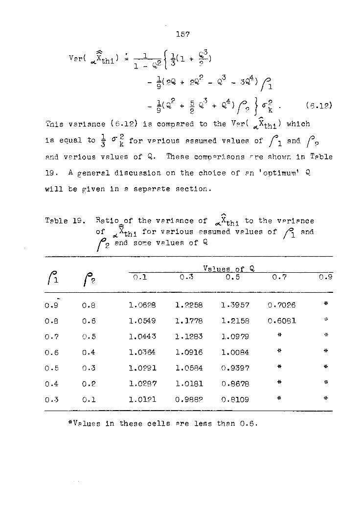
157

Var( _Xthl) : _i 1 _ I 3

1(1 ft' ;3.

• )

- (24 + 2%^ - - 3Q-)

- K + § « * + »4)fo } ' I . (5.1?)

This variance ( 6.12) is compared to the Vpr( X^^) which

is equal to j for various assumed values of j° and j°9

and various values of Q. These comparisons "re shown in Table

19. A general discussion on the choice of ?n 1 optimum1 Q

will be given in a separate section.

Table 19. Ratio^of the variance of ^X^^ to the variance

of ^thl for various assumed values of an<3-

^2 an<^ some values of Q

A A o.i

Values of 0, 0.3 0.5 0.7 0.9

0.9 0.8 1.0628 1.2258 1.3957 0 .7026 *

0.8 0.6 1.0549 1.1778 1.2158 0 .6081

0.7 0.5 1.0443 1.1283 1.0979 * -*

0.6 0.4 1.0364 1.0916 1.0084 #

0.5 0.3 1.0291 1.0584 0.9397 * »

0.4 0.2 1.0287 1.0181 0.8678

0.3 0.1 1.0121 0.9882 0.8109 * *

*Vpiues in these cells pre less than 0.6.

158

B. Estimate of Visit-to-Visit Change,

from the i^^ Primary o(.- lXth>

1. Struc ture

To estimate the visit to visit change, ~ o<-lX

th aC-X th

(6.13)

with the use of the 1 psu, consider , 55-

odDthi = *Xthi " -lXthi

which is the difference of the composite estimates at the =c

and ( oL -i) visits. From (6.1) and (6.?a), (6.13) becomes

o(Dthi = %

Letting

and

( et-l)Athi " ( -t-53) Xthi^ (+ ( ajthi ~ (=c-l) Vthi^

<*-lDthi = ^-lxthi " ^-oxthi »

«Zthi = <*Vthi - ot-iVthi »

we have from (6.13a),

*.Bthi = G o<-lDthi + ^Zthi

(6.13a)

(6.13b)

(6.13c)

(6.14)

which is similar in form to (6.°). We can, therefore, write

(6.14) as

*Dthi v=0

,v oc -v thi

(6.14a)

and its variance is

159

Z Qr Cov( zthi'^-rZthi^ 1 - Qs ,

r_1 (5.15)

2 . Variance

The variance of ^-^thi evplupted by term by term i

evaluation of the variances and covariances of the ^^thi'^*

But the thi ' pre functions of the ^thi ' s and we c?!n

utilize the results given in Tables 1? and 18.

Using (6.13c), (5.7), and (P.8), the first term in

(6.15) becomes

Var( otzj;hl) = 11( P + PQ + |q?) - 1(4 + 13Q + lOQP)/°1

+ 1(Q + 1% ) 1°. ( 6.16)

Similarly,

oczthi» <*-lZthi = 3(1 " pCl "

+ jg( ? + 17Q + 50, ) - Yg( P + 50, + ?Q9) (°»

(6.17)

Cov( * Zthi> cc-PZthi) = [3^ ~ - §(P + 0, - Q?)

+ 9^ + ! (6.18)

Cov( *Zthi> 04-3Zthi) = [e^1 ~ 1 ~ 9( 1 ™ pC: ™ p^?>)C

(6.19) *1

and

160

c°v( Âl> «-v^hV ' 0 (s-'0)

for

4 6 V ± e>c .

Using equations (6.16), (6.17), (6.16), (6.19), and (6.90)

in (6.15) and simplifying, we have

Vsr( oc^thi ) - ^ j" ^(1 ~ 4^ - $ -

- j|(4 + 5Q - 3<T - 4Q'3 - 5Q4 + 3Q5)

+ ^ ^"k '

This variance is compared to the variance of

*Dthi = *Xthi ~ ^-iXthi (6.9?)

which is the difference between the regular unbiased esti­

mator at the ol visit and at the ( *( -1 ) visit. The variance

of Âhi is

Vsr( Dthi^ = 3(l " |/>1) k * (6.99a)

The comparisons are given in Table 90, for various assumed

values of y°-^ and and various values of Q. The choice

of an 'appropriate' Q will be discussed in a later section.

If the variance of is compared to the variance of

o<.Dthi ol , pC -]Xthi ^-1, oc Xthi (6.2?b)

which is equal to

V*r( = (1 _ /*i) (6.9Pc)

then some changes will be made in the values p-iven in Table

161

Table 20. Ratio of the variance of ^thi the variance

of ^ thi for various assumed values of and

P0 and some values of 0. « r

Values of

/I A 0.1 0.3 0. 5 0.7 0.8

0.9 0.8 1.1655 1.6162 3.8131 7.3665 •if-

0.8 0.6 1.0846 1.3330 9.04-69 3.2659 *

0.7 0.5 1.0844 1.2505 1.6903 9.4956

0.6 0.4 1.0672 1.1820 1.4395 1.9835

0 • 5 0.3 1.0461 1.1420 1.9711 1.7930 *

0 .4 0.2 1.0366 1.090? 1.1746 1.5383 8.7090

0.3 0.1 0.8116 1.0431 1.0907 1.38so 3.6364

Var( aVplue of «tDthi) *re

Q = 0 .9 is negative.

omitted since the coefficients in

^Coefficients in Vpr( .Xhl) are negative.

20. These changes will depend on

a) If /°i = then Var( o<Dthi^ = ^ar( Dthi^ snâ the

values in the table remain the same ;

b) If (°i < then Var( Dthl) < Var( (<D^hi) and the

values in the table will increase; and

c) If 1° 2 > then Ver( Dthi) )> V?r( and the

values in the table will decrease.

16?

C. Estimate of Vislt-to-Visit a Year Ago Change, etXth ~ »<-?xth > from the i^h Primary

1. Structure

To estimate the visit-to-visit a year ppo change, -

<<-?Xth> us consider,

oCDthi = *Xthi ' *-9Xthi ' (S.?3)

From (6.1), (6.?3) becomes

oCDthi " -lXthi " «*-3Xthi^ * ( <<Vthi " ^-P^thi^ '

(6.P3@)

Let

*-lDthi v_ixthi " ^-3Xthi « (6.?3b)

and

*Zthi - *Vthi " «k-?Vthi ' (6.?3c)

then we have for (6 .?5) ,

*Dthi = Q ^_iDthi + <kZthi (6.?3d)

which is of the same form as (6.?) and, therefore, we can

write it as

eL Dthi = X „<_vZthi (p.°3e) v=0

where M

Zthi sre functions of Vthl and rJthi •

163

2. Variance

The variance of ^D-thi ls Fiven by

mDthl> = " - Var( „<Zthl)

— +

^ 1 - 1 -

£ • (6-"4) r=l

The variances and covariances of the ^ Zthi'^ Pve evaluated in

the same manner PS the corresponding variances and covariances

of the ^ zthi's ' Thus>

V9r( c<?thi) = 1 -

1(1 + iQ° - Q, - IQ") 3 4 4

- l(oQ + 8Q?' - 6Q - HQ" + ÇT + 3<T) y°

|(P _ Ç, _ OQ* + |q3 + Ç4 _ 5Q 5 - Q 6 ) y l - •

(6.?5)

This variance may be compared to the variance of

J^thi = **thi - k-Âhi (6.P6)

which is

Vsr( Jthi1 - f ( i - V , i rk • (6-?6a) /? ?

The pain in precision in the use of ^ thi to of u

Dthi

for various assumed values of and and various values

of Q is given in Table 21. »

If the variance of ocP^i is compared to the variance of

n* Y X ^^thl = ^ , _2^tHi - ^-2,^ thi

164

Table 21. Ratio of the variance of ût^thi to the variance ol

D " oi thi for va rious values ; of A ?nd ^ and some

values of Q

A Val ues of Qp

A 1 f? 0.1 0.3 0.5 0.7 0.8

0.9 0 .8 1.0848 1.354? 1.7393 1.7568 1.3984

0.8 0 . 6 1.0744 1.P539 1.4993 1.3516 1.1589

0.7 0 . 5 1.0613 1.1930 1. ?8 59 1.1747 1.036?

0 . 6 0 .4 1.0508 1.1383 1.1551 1.0383 .9300

0 . 5 0 .3 1.0379 1.0866 1.0651 .9284 .8497

0.4 0 .? 1.0208 1.0387 .9849 .8465 .7788

0.3 0 .1 1.0181 1.008? .9975 .7849 .7258

aAll ratios for Q = 0.9 ^re less than 0.6.

which is equal to

Var( J^hl) * ?(l - /%) ,

then changes in the values given in Table °1 will be made

depending on the following:

a) If l°2 = then Vsr( ^thi^ = Var( ) and the

values in the table remain the same; _ A A

b) If r> < then Var( Dthi^ ^ ^ar( ^thi^ ?na the

values in the table will increase ; and

If /% >!' then Var( DtM ) ) Var( Jc*hl) and the

values in the table will decrease.

165

D. Sector Estimate

To estimate the sector total, otxt, we need to evaluate

the estimator of the stratum total, ^^th» from the five

ordered psus or mean of the five psus. Similarly, we have

to evaluate the stratum visit-to-visit change and visit-to-

visit a year ago change estimates from the five ordered psus.

To do this, we invoke the results of the theory presented in

Chapters III and IV by identifying ^xthi' *Dthi <*Xthi '

The results will be summarized for the mean of the five nsu

estimates.

The stratum estimates are as follows:

a) Current total or level, ^X^h

Estimator : (6.P7)

i

where ^xthi ?s defined in (6.?) and m = 5. A

Estimate of variance: To estimate Vgr( =

m

i

c ) Visit-to-visit change, ^Xth -

Estimator: (6.9%)

1

where ^^thi is ps defined in (6.13).

166

Estimate of vpriance: To estimate Var( ) =

we use m

2 x o

^ th = râ ri - 1 *Dthi ~ =tDth^ ' (6.?8a)

i

c) Visit-to-visit a yepr apo change, ^ xth ~ <xr-°Xth

Estimator: = i Xhi (6'?9)

i

where ^ ®thi is ps defined in (6.93).

Estimate of variance: To estimate Vpr( ) =

IîiIXmI, we use m

c?th = m m - 1 S ( eCDthi " »<Dth) ' (6.99s) i

The estimates for the sector are as follows:

a) Current total or level,

\ - * > - ^ Egtlmetgr: Jt = 1 g Xu (p.30)

1

where *tl = 5Z Xhl •

Estimate of variance : To estimate Var( X^. ) =

ïar(^Xtl) Ji±—, we use

m

2.9 , i V"*5 a a p Zt = ï tTTÏ A, ( tl - ^Xt)' . (6.30,)

i

167

b) Visit-to-visit change, ^X^. -

Estimator: ^ti (6.3l)

^thl ' h

where D^i = ^

Estimate of variance: To estimate Var( ) =

Var( D' ) Jii_> we use

m

/\ = i —1— ( D' - Dl)? . (6.31a) t m m - 1 —' c< ti oc t

i

c) Visit-to-visit a year ago change, ^X^ -

Estimator: X * m S' *Dtl (s"3s)

i

where = ]T Dthi *

h ii,

Estimate of variance: To estimate Vsr( ) =

Var( ) -, we use

m

2

i - x > - ( s - ^ > v ^Dti -i

With the use of the above techniques, estimates for the

whole rural area (t = 1 and t = ?) may be obtained. If there

exists a systematic correlation between the primary numbers

i = 1, i = 2, ..., i = 5, then the short cut method of esti-^ p a

mating the variances, jy\, and is an over estimate

and as such the standard or 1 stratified1 method should be

168

used.

We can also apply the ratio estimation techniques devel­

oped in Chapter V to the 1^ psu composite estimate, xthi

(6.1) for the strata and the ith psu composite estimate,

X^ (6.30), for the sector. With these correspondence,

four ratio estimators may be derived for the sector:

a) 1 separate biased ratio of means estimate' which is

similar to (5.33),

b) 1 separate unbiased ratio estimate' (5.63),

c) 1 combined biased ratio of means estimate' (5.38), and

d) 1 combined unbiased ratio estimate1 (5.66).

This approach is simple since the Z variable is presently

available by precinct, by stratum and by sector. In this

case, we have composite estimation first and then ratio esti­

mation .

E. Choice of an Appropriate 0,

In a general purpose survey like the PSSH where hundreds

of items are processed, the practical approach is to choose

a general Q which will result in a reduction of variance for

most if not all of the important items in the survey rather

than finding an optimum Q for each of the characteristics

covered in the survey. This approach becomes more advan­

tageous when we consider the fact that we are interested in

using three types of estimates, namely : current total esti­

169

mate, estimate of visit-to-visit change and estimate of

visit-to-vist a year ago change. Each estimator end its

variance are functions of 0,. The choice of 0 will, therefore,

depend on the reduction of variance for most items and also

for the three types of estimates.

The U. S. Bureau of the Census in its current population

survey (CPS) uses a value of for Q {jioj for the within psu

variance of composite estimate. This choice of Q results in

smaller variances of estimates of both level and change for

most characteristics, but larger gains are achieved, for most

part, in the estimates of change. Experience of various

authors [?, 10 j seem to indicate that for most items,

2 - I 1

i.e., the magnitude of the correlation decreases as the length

of the visits increases. In the PSSH, the correlation

six months apart of estimates from identical segments and

is the correlation 12 months or one year apart of estimates

from Identical segments. The correlation six months apart

of estimates from identical precincts (psu) of population

in interviewed hhs, ^_xthi> for the first seven strata in

urban Manila is estimated at about 0.9 and the correlation 19

months apart of estimates from Identical precincts (psu) is

estimated at about 0.8. These correlations are expected to

be high since the estimates are for population counts from

identical precincts (psu).

170

From the results in Tables 19, 20 and ?1, one may obtain

an idea on the appropriate choice of Q for estimating current

total, visit-to-visit change and visit-to-visit a year ago

change. For Ç*2- 0.5 and corresponding j0^ ln the tables,

fairly large gains in precision are obtained for the three

types of composite estimates for 0.3 - Q ~ 0.5. Empirical

studies on the magnitude of ^nd ^2 of estimates for the

most important items in the survey will be msde in order to

indicate the choice of an appropriate Q for use in the PSSH.

F. Finite Population Approach

After segmentation of the sample barrio in a given

municipality, the segments are arranged at random into a

rotation pattern. The number of segments, ^, in the

sample barrio is usually small,

4 - sthij - 10 •

Consider a particular rotation (R) for j = 5 which is

given in Figure 2 for some < • Our main interest is the

estimation of the thij^h barrio total at time 0, Q^thij•

Since is small and with

- <* •= oC £0

our finite population will consist of the possible R' s

from which we have drawn a sample of size one. In our

example,

Sthij = 5

171

Time . c* number -6 -7 -6 -5 -4 -3 _9 -1 0

1 X X X X X X

? X X X X X

3 X X X X X

4 X X X X X

5 X X X X X X

Figure ?. A particular rotation pattern for sthij = ®

and our finite population is the 5! R's. The sample R may

have the pattern given in Figure ?• The usual method in the

estimation of QXthij is to draw the 3 segment out of the

Sthij segments at time 0 and consider the finite population

consisting of the

'S.

possible samples, and for j = 5 this is

( I )

possible samples of size 3. In the present model, the sample

consists of one sample R from the possible 5I R's.

17?

1. Structure of estimate

Assume that the same sample of hhs is observed in a

given segment for any time and that there no 1 drop­

outs1 or additions or replacements of households. Consider

as composite estimate of the thibarrio total at time 0,

0Xthij

« 5 xs = ^ ' 53 wthijk ocXthijk (6.33) 0 thi J

=0 k

where

,<Xthi jk - ^ <aCxthl is the sample total estimate thi j k

of the thljk^ segment at visit ot ,

Nthijk is the number of hhs in the thij^ segment and

is independent of ,

nthijk is the number of sample hhs in the thljsegment

and is independent of c< ,

<sdxthijk ls ^he sample total of the thijkth segment at

time oL ,

«KVthijk ls the weight attached to the ^%thijk ¥-,r

time < t

and

Sthij = 5-

One substitutes sthlj for 5 ln the following derivations in

order to express the results for a general S^^ij where s-thij

is small. The weights, ^^thijk» in (6.33) will be determined

173

from the relation

0Xthlj = ^-lXthij + 0,-l*thlj - -l,0%thlj) + (1 - o\hij

(6.34)

where

^ t h -lXthij the composite estimate of the thij barrio

total at time -1, _1xt;hij '

0,-lXthij = | (o^thijl + O^thijp) (6.35?)

is the regular unbiased estimate of g^thij based

on the two matched segments for times 0 and -1,

-l,OxthiJ = | ^-lxthijl + -lXthiJ?^ (6.35b)

is the regular unbiased estimate of _]_xthij based

on the two matched segments for times -1 °nd 0,

^ 5 z A 0Xthij = 3 0Xthijl + 0Xthij? + 0Xthij3) (6.36)

is the regular unbiased estimate of QXthij based on

the three segments at time 0,

ana

0 £ Q, ± 1 .

A Using equation (6.34), _^Xthij Tra^ expressed in terms of

^ -A A A

-2Xthij' -1,-PXthij > -?,-lXthij snd -lXthij' In general

(6.34) may be written es

0Xthij = YZ % * thijk (6.37)

V=0

where

c i , ec-lXthijk - eL-l,*. hijkH1"^ »cxthijk-

174

For any particular H and for s given time << , the weight of

a segment total estimate, xthijk' will depend on whether the

segment is in the sample for the first visit, the second

visit, the third visit, off one visit or off two visits, etc.

These weights are shown in Table 29 for ^t:hij = ® f°r

oC - o, o(_ = -1, oC - —, oL - ~ 3} and oC = —4. From the pat-

term of the weights in Table 92, we can say that for a given

time ^ < 0, the weights are

_ a or (q +1) (*.38e:

for a segment in the sample for the first visit;

ê QT (Q _ i) ( s.38b) 6

for the second visit;

| QT * (| +• 1) (6.38c)

for the third visit; and

0 (6.33d)

for a segment off one visit or off two visits. a

The expectation of Q^hij

E(0*thij' = !,RfE(OfthlJ I *>} (6.Î9)

where

E(o^thij I Is the conditional expectation of o^thij

given a particular R,

and

E is the expectation over all 5'. R's. 5'.R

Table 2 2 . Weights of segment total estimates depending on whether a segment Is In the sample for the first visit, second visit, third visit, third visit last time, third visit second to last time for = 5 and for oi = 0, -1, -?, —3, -4 for a particular rotation

Segment in sample

for - 0 oi= -1 o(. = —P o(, = — 3 oC - —4

1st visit - |(k. - 1) - §^(Q + |) - |QP(Q +1) - |Q,-5(Q + 1) - |Q4(Q+ 1)

Pnd visit 3^ s + "6^^ ~~ ^Q^(Q. - l) ^Q^(Q - 1 ) ( Q - 1 )

3rd visit + l) 3^? + §Q.^(§ + l) §Q^(§ + l) ^Q4(§ + l)

Off 1 visit 0 0 0 0 0

Off 2 visits 0 0 0 0 0

5

5 53 aj'thljk. 1

k

0 0 0 0

176

To evaluate (6.39), T-re have

E fE'"°

5'.R ZZ ZJ c<wthijk ^thijk o< =0 k

R

— oO

= E 5'.R

yi yi y thijk e( ^thijk^j <k =0 k

-<0 5

-«IS? ' thijk Xthijk

where

th ^Xthijk ls the thijk segment total at ti

Finally, ( —m 5

SIR (2^ X «'WV L oC= 0 k

- oo 5

= ^ r IZv ^IR( J^thijk) Xthijk

x=0 k b,rt

- 0Xthijk

0Xthij

where

. th O^thij is the thlj barrio total at tire 0

G Xthijk) = 1

for oC = 0, and

E,r( ^thijk'' = 0

for oi < 0

177

* This result shows that oXthij is unbiased. The expectation

of the o^^thl ik over all 51. R' s is obtained from the fact that

each of the five serrent totals, ^xthijk» spears for a riven

oC in the five categories in Table °? an eoual number of times

which is 4'.. Thus the expected weight of ^Xthijk obtained

from the relation,

which is given at the bottom of Table 9? for some << . Note

that the summation on k is taken over the five categories

into which the five segments fall on a given time <*. . In

general, the number of categories is equal to the number of

(6.45)

we evaluate the terms in (6.45) separately. The first ter™ is

oc thijk

(6.44)

segments, Sthij •

2 . Variance of composite estimate

The variance of QXthij is given by the relation,

thijk * thijk

thijk thijk

5

+

(6.46)

178

where

— ta 5

V?r(o^thij I - 53 Yh ^Wthljk Vpr^ thijk^ o(=0 k

—oO 5

5Z Y2 thijk ^thijkCov( thijk' oC'xthijk) -

k (^.46a)

«Sthijk = Ç l**thl,1k/~ i^hilkL ,

* Nthi'k - 1

YL «Ahijkl

^Xthijk = Ntwjk

Cov< ^,Xthijk) • Sir(1 • Sï^.^^hijk

(6.46c)

end

oC , oc' Sthijk

Ç ( *xthijkl - ctXthijk)( ^'%thljk - ec' Xthijk)

Nthijk - 1

9 The values of ^thijk or ~ 0 ?nà for e>^<0 for a

given R are given in Table 9-3. From this tsble, we c^n

evaluate

g I R( ^"thijk' ' (3 ^ PP) (6'47)

for cC = 0; and

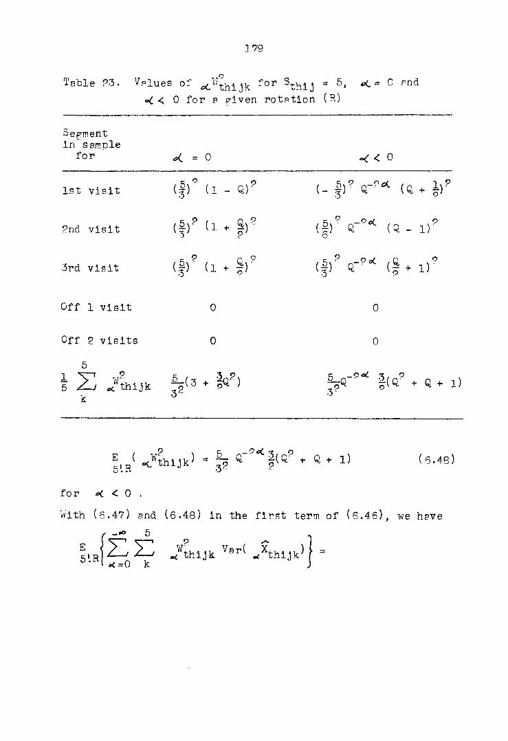
3.79

Table P-3. Values of oi^'thi jk for Sthlj = 5> <<=0 and

<< < 0 for a given rotation (R)

Segment in sample

for a(. = 0 ^ < 0

1st visit (§) (1 - Q)' (_ or?* (Q +

?nd visit (|)P ti + lv (§> cr"* ($ - i)p

•3rd visit (§)• (i . #) <ff a-"" (| • Dc

Off 1 visit 0 0

Off 2 visits 0 0

5 Zv oc'thijk k

^=(3 + go?) 3S

#(Q% Q+ 1) 3-

^IR( o<.WthiJk^ = §? Q + Q + l) (6.48)

for K < 0 .

With (6.47) and (6.48) in the first term of (6.46), we have

f~*° 5 Z13 Xijk v"< Jthijk' x=0 k

180

5

53 !, Jo1''thijk' VarVthijk' k 5'H

-eO 5

+ 53 53 G ( ^thijk^ Vpr( Âhijk)

4 = -l k

3? [ 5T • p- ' lo"thijk

k

— & 5

5

(-3 + ^Q" ) V>r(~X., . ,, )

+ 23 S | ^ + 1) VPr(

od = -l k

Equation ( 6.49) may be simplified if T-Te assume

Ver(o%thljk) = «%thijk)

for all , and let

— eO

H « -2X. Q?

«<=-1 1 - ^ '

After some simplification, (6.49) finally becomes

—5

E 51R S 23 J^thijk Vsr( «Ahijk)} = ^=0 k J

gë Z Ver(oXthljk) '

The second term in (6.45) is

181

- °° 5

?.R| zL 5Z xWthiJk-^ti'thijk Cov( *Xthijk' 'Xthijk^j

5* 1 a** k 1

-oO 5

= ?53 23 E^( 0<Wthijk'oC_lWthijk)Cov{ Âhijk' od-l^thijk^ o<-0 k

_ °o 5

+ 2 53 X" gIR( *thijk' *-2V''thijk)Cov( ^thljk' c-P^hij^

*6=0 k b' (6.51)

where

Cov( «cXthljk» *-vXthijk^ = 0

for v >. 3.

To evaluate

5,r( Aiijk ^,Wthljk)

for oC oC* , we use the results given in Table pnd the

weights given in ( 6.38a) to (6.38d). Thus,

^IR(0'Vthijk -lWthijk) =

1 5

(3) ( p + 1) ( -j)Q,(Q + + (^) ( •+• l)(g-)Q(Q - l) | ;

(6.59?)

^,R(0Wthijk -PWthijk) = e>[(3)(§ + l)(-|)Q" (Q + |) J ; (6.52b)

^,R( *Wthijk «^.-lwthijk) =

cL < 0

(§)&-*-(% _ l)(_§)Q-* + l(, + 1)

+ (^)Q, ^(g + l)(g)Q ^(0. — 1 ) ; (6.52c)

18?

snd

^thijk <-Ahijk) = sft 3)^^(9 + !)(-§)% + 1)}.

< 0 (6.5?d)

Substitute (6.528), (5.59b), (6.59c) and (6.59d) into (6.51)

and assume that

Cov^ u Xthi jk' „<-lXthijk^ = /°1 Vpr^OXthiJk^ »

C°v( *iXthijk, o<.-?Xthijk^ = /% V?r(0XthiJk^

for all o£ ± 0, where

/\ is the correlation of estimates from identic?! seg­

ments one visit apart,

and

j° 2 is the correlation of estimates from identical seg­

ments two visits apart,

then after some algebra (6.5l) becomes

- aO 5

E ~ ~r wthijk ¥thijk Cov thijk» Xthijk J 5'.R[ -v <

-a** k

- 2 ( f s } r z n ? f ( ( i + q S • K - 1 ® 4 ) / ° i 5

+ |(ftS + If + V*"VthiJk> • <5-55)

With (6.50) and (6.53) in (6.46), we have

y Wmj I ^ + j

- ? [(Q + Q,P - iQ3 - |Q4)

- + fft3 + j°pjl %% Var(oxthijk ' (6.54)

183

This is the within rotation variance and the leading term is

(6.55)

which is the within segment component for ? two-stage sameling

with equal probability snd without replacement ?t each stage

at time 0. For small the within segment component is

usually the more important.

In the U. S. Bureau of the Census publication, the within

psu-variance of the composite estimate is similar to that of

equation (6.4) or (6.12). The between-psu variance is the

same for the composite estimate as for the regular ratio esti­

mate. The reduction in variance through the use of the com­

posite estimate is entirely in the within-psu contribution to

the variance. For many items the within-psu variance is the

principal component to the variance of month-to-month change,

the gains on estimates of change are worthwhile.

The variance in (6.12) denotes the variance of the

straight estimator of the stratum total, from an indi­

vidual segment. The within psu variance of this estimator

will in general have a between segment and within segment

component. Thus,

« I - "1 - 'I •

We shall now identify

184

p v

-î| with 6* 1 53 Vpr(0Xthljk)

c k

in equption (6.54) where

B le the general raising factor for the stratum or is

the number of barrios in the stratum.

It will be seen that the factors applied to these two Quan­

tities agree.

The second term in (6.45) is

Vfr{E(0Xthij |S)j = EiH{E(0XthlJ | R)f

A ?

" {E J^Vthij I R']| • (6.56)

Note that the second term on the right hand side of (6.56) is

evaluated with the use of (6.41). Thus

[E<0*1fclJ lR>]}° = {oXthij]? • (6.57)

The first term in (6.56) becomes,

— ob 5 o r ~ 5

E 5',

— ot> 5 p r — 5

/thijk ^xthijk] = ®,R}ZZ Yj /thijk /thijk ^0 k ' -<=0 k

— oo 5

+ 53 Z Jthijk /vVthijk ^thijk ^'Xthijk

— oO 5

^ thijk ^ thijk' ^thijk *'thijk' + 1 '/ Wt.h 1 1 tr Wtln1 llr' .X-Hn1 llr -Url

c i = 0 kfk'

- ot> 5

Ï-J X3 "thijk ''"thijk' xthijk ,xthijk'}. -et*' k,k' * " * Is.58)

185

The four terms on the right hand side of (6.58) pre evaluated

separately. The first term is

— 00 5 — 5

2 l/C 22 J thijk /thijk j Z Z IR( /thijk* /thijk

5-HL^=0 k J ^=0 k 0

(6.59)

With the results from (6.49), (2.59) becomes

g , R[ë 2D /thijk /thijk] = f?|è (' 3 + ? Q ^0 Xthijk oC=0 k J * k

+ (?-69s)

^=-1 k

where the infinite summation is truncated to include terms

involving —3 6 d ± 0. The second term in (6.58) is

-•o 5

oC *oc k

( ~ 5

5>RI 213 /thijk ^,¥thijk /thijk JXthijk]

- 2ZT ZZ E ( /thijk 1 V'thijk /thijk ' Xthijk * 1 v °*

** * (6.60)

Equation (5.60) is approximated by truncating the Infinite

summation. Thus,

® J 53 23 /thijk j "thijk /thijk «,xthijk| = 5 ***' k i

- + ?e,oxthijk -lXthiJk

186

R

+ V (a5 + ft4 -0XthiJk —3 thijk

k

5

+

ci=-1 k

-1 5

- e ° + § > * w . A h i j k

- TZ YZ « <« - F + ^)<%thijk -Ahijk l ai =0 k i

,rSe< m4 . 5?% °-

=0 k

( 6 . 6 0 ? )

The third term in (6.58) is

— cO

E olR

— CO

J3Z3 /thijk /thijk' /thijk /thijk' 1 I 0 k*k' J

" 5Z5Z E ( /thijk /thijk1 ) «/thijk o/thijk' ' ^=0 k*k' dlrt

(6.61)

Kow

^IR(0Wthijk O^thijk') = 9 Jp ( 3 ~ |Q j («.61e)

and — P°C

5'R^^thljk /^thljk' ) = ~ % + ^ + l)) •

oC < o (6.61b)

With (6.61s) and (6.61b) in (6.61) snd truncating the in­

finite sum, (6.61) is approximated by

197

~ 5

E Z_v 2-3 /thijk Wthijk' /thijk /thijk' } = v•" <<=0 k*k' J

5

? fg X3 (3 ~ I44 )0Xthijk 0Xthijk' k*k

- & %3Z3 ^ + i)«<xthijk <xthijk' -'5 ^ = -1 k*k'

( 6 . 6 ? )

The fourth term in (6.58) is

- op 5

E ' HJ /'thijk '-''thijk' ,Xthijk ^'xthijk' 1 s'.R) «

— oO

' =.R /thijk /"thijk' ' /thijk /^thljk' ***' k+k' D'n

(6.63)

Equation (6.6-3) is simplified by truncating the infinite sum.

Thus, (6.63) is Approximated by

-3 5

JZj C /thijk 1 âthijk' ) /thijk JXthijk' " o k * k '

-2 5

C Z3 % ( /thijk cK-lWthijk' ) xthijk *-lXthijk' /=0 ktk' °-H d

-1 5

+ X3 Z3- E ( /thijk x_p%thijk')<Xthijk *f-?Xthijk' x=0 k*k' n

5

+ X3 E (0Wthijk _3wthijkl Wthijk -3Xthljk' * (6l64)

k*k' 5lrt

188

To evaluate (6.54), the following expectations are derived:

•3

^,R((/thijk -l^thijk') = ? 4- + ^ + GO ' (5.64a)

g.^O^thljk -Wthijk') = P ^(9- + + P") ' (6.64b)

^IR(0V'thijk -3Wthijk' ) = 9 §P^?~ + t~ " ' (6.64c)

^,R^-lVj thijk -nWthijk' = \ JQ* (4- " §~ + 4) » (R.64d)

g,R(-lV/thijk -3V;thijk' ) = i JôqP(T~ + 4^ + » ^6.64e)

5,R(_/thljk -3*thljk') = ? (4- - #- + 4) ' (%.G4f)

With (6.64a) to (6.64f) in (6.64), (^.64) is approximated by

— cb 5

E 5'.R

W. oC

•itcC kfk thijk /^thijk' /thijk ^'Xthijk' j =

3 9

+ Q, + Q.)0xthljk _iXthijk'J

1{P~ + !q3 + t~)0Xthijk -/thijk'"]

+ _ Q,- )0XTHLJK _3%thijk']

of ^ Q\ y y . p [T~ ~ ~ + r-Zthijk -/thijk']

|V(§- + |q3 + §-)_i%thijk -3Xthijk'

[^(4" - " 4)-9Xthijk -3Xthljk'] j ' ^'^)

189

With (6.5?), (5.59e), (6.60e), (6.6?), (6.65) In (6.56)

and after some simplification (6.56) finally becomes,

(oxthij I H)} 1 f-(| + K >0Sthij

-3

! YL (l' * e > 1) ,s; 3 Z-, '5' " " T „cJthiJ o( = -l

-1 f(r + Ie + 'o,-isthij

-1 ¥¥ * ¥ - ^3>o,-ï*thij

o( =0

-I £ <^6> e(=-l

where

*.Sthij " ^thijk " * 5h1,1

X. *-vsthij = 4 j *Xthijk <-v%thijk " * thl,15" V th1,1

and

oZXthij = 53 ocXthijk • k

At Q = 0, equation (6.66) becomes

5P P q5 3~ 5 OsthiJ

190

which is the between segment component in a two-stage sampling

scheme with equal probability and without replacement at each

stage at time 0.

With the use of (6.54) and (6.66) in (6.45), and with

rearrangement of terms then,

Vsr(oxthij> ; I^ [(3 + §«3> - "(a + <f - 1q3 - fe4)/0!

5

_ (0% + |Q3 + Q4) °pj 2_j Vflr(oxthiJk j v J k

• S-J (§ • iQ s )0s^h l J • X2 i <Ta" <e? + c -+ 1) Ans

P(=-1

£ 3

" P 3 [(9,3 + 4QÎ? + 4Q)0,-1S thlj

-1

oi= 0

oL =—1 p

The Identification of the corresponding terms for the ^

component in d* with the second part of ( 6.67) is more

difficult.

191

VII. SUMMARY AND RECOMMENDATIONS

Development of multistage designs for statistical surveys

in the Philippines is presented. These surveys are collec­

tively known as the Philippine Statistical Survey of House­

holds (PSSH).

The present basic design of the PSSH (Chapter III) is

known as multistage with complete replacement of primaries

(psus). The psus were drawn with pps In the rural area snd

with equal probability in the urban area. Five numbered psus

were drawn from each stratum. The stratification techniques,

methods of sample selection and details of the methods of

estimation are described. To simplify the estimation pro­

cedure for totals, a self-weighting estimator is utilized.

In order to make the self-weighting estimator unbiased, apart

from rounding errors, two restrictions were imposed on the

design. These were the conditions on R^, the overall raising

factor for the tth sector (t = 1,2,3,4) and on f^i» the thith

psu constant for the rural areas (t = 1,2) or on f the th**

stratum constant for the urban areas (t = 3,4). Since the

psus were drawn with complete replacement and were numbered

for each stratum, the estimation of variance of estimate

consisted of the same ordinary sample variance form for the

stratum, the sector and for the whole country.

If the numbering of the psus, 1 = 1, 1 = 2, ..., 1 = 5,

-x P is independent and at random within each stratum, then <r~ ,

*t the 1 short cut method1 of variance estimate of the tth sector

19?

( t = 1, ?,3,4) is unbiased, but of a rsther low precision since

it is computed from only 4 degrees of freedom (df) for any

given sector. On the other hand, the standard or 'stratified1

variance is given by

h

and is computed from a pooled 4 L% df since each stratum esti-

mate s^ is derived from 4 df. An analysis of variance is

presented to indicate the differences between the two esti­

mates of variance. If a systematic correlation existed be-

x ? tween the numbering, i = 1, i = ?, ..., i = 5, then <T^ will

be an over estimate, since a component of variance is intro­

duced into the between primary number source of variation.

For the May and October, 1956 rounds, the 1 short cut1

method of variance estimate, <J"5^, was found to give con­

sistently higher estimates than the 'stratified1 variance, p s^, in the rural areas (barrio and poblacion sectors) but

consistently lower estimates in the urban areas (capitals

and cities and urban Manila sectors). Some systematic bias

may have been introduced into the initial numbering procedure

of the psus within strata.

Under the requirements of the present basic design of

the PSSH, the same panel, except for minor replacements, of

sample hhs in the sa (barrio, poblacion or precinct) is inter­

viewed from visit to visit and a complete listing of the

193

number of hhs In esch se Is executed for every visit. These

requirements resulted in increased 1 response' resistance from

panel hhs snd in a relatively high cost of listing. To remedy

these situations, a segmentation procedure of the sa is intro­

duced and a rotation scheme is developed and instituted into

the basic design (Chapter IV). The sa (barrio, poblacion or

precinct) is dissected into three or more segments and then

the segments are arranged in rotation groups. In general,

esch rotation group consisted of three segments; two segments

or 67 per cent of the segments were common from visit to visit

and one segment or 33 per cent was common from year to year.

A given segment was in the sample for three consecutive visits

and then dropped from the sample. The basic idea is to split

the barrio or poblacion (ssu) and the precinct (psu) into seg­

ments and to carry out the listing operation only for a sample

of three of the segments to be rotated from visit to visit.

Thus the cost of listing is reduced inversely with the number

of segments in the ss. This technioue of segmentation and

rotation is found to be feasible and applicable in both rural

and urban areas. The rotation scheme is expected to reduce

'response resistance' of panel hhs.

The segmentation of the sa and the subsequent listing of

only three segments in a given rotation group reduced the cost

of listing from 15 per cent to about 6 per cent of the over­

all field cost. In addition, the introduction of a simplified

194

field operation which eliminated a second visit to the sa for

the actual interview, resulted also in a reduction in cost of

the return travel for the actual interview of sample hhs.

The sampling rates within segments (srws) are adjusted

such that the regular self-weighting estimation procedures are

retained in the design. Equal srws is used in the urban areas

and in the poblacion sector of the rural areas whereas unequal

srws is introduced in the barrio rural sector. An attempt is

made to equalize the size of segment in the urban ^reas and

in the poblacion sector. This technique introduced some con­

trol in minimizing the between segment component in the urban

area estimates of variance. Equalization of size of segment

was not feasible in the barrio rural sector. Thus, unequal

srws but equal take in the number of sample hhs is used in

the barrio sector design. This technique is expected to pro­

vide some control on the variation of estimates from visit to

visit and has the advantage of having eaual work loads within

segments.

To improve the barrio sample and to bring the barrio

sector estimates, particularly those for the region to a

higher level of precision, an attempt was made prior to the

segmentation procedure to control the variation in the size

of the barrio through the equalization of size of population

in barrio. This redefinition of the barrio brought about

considerable reduction in the coefficients of variation of

195

regional estimates for the barrio, the barrio sector and the

whole country. These aspects of the PSSH design are discussed

in Chapter V.

In the urban area, the psus were drawn with complete re­

placement and sampled at each stare with equal probability.

There is a slight loss in precision represented by not apply­

ing the finite population correction and a larger loss in

precision arises through sampling the psu with equal prob­

ability.

To increase the precision of estimates in the urban

areas, ratio estimation is introduced into the urban design.

This is discussed in Chapter V. It was noted that an auxi­

liary variable, Z, the count of registered voters which was

correlated with population characteristics, is available by

precinct, by stratum and by sector with little or not cost to

the survey. The survey urban precinct was identical to the

registered voters precinct. The i * psu estimate, ^^thi» of

the stratum total, ^^th» the °L visit is assumed to be a

random observation from an infinite population of such esti­

mates . The same assumption is made for the i^*1 psu estimate

of the Z variable. Thus standard techniques of ratio esti­

mation are applied with the i^ psu paired estimate, say,

( %thi, zthi' 88 the 1 pair of random observations. Three

forms of ratio estimators for population in listed hhs and

occupation of head of hhs were available, namely:

196

s) complete ratio estimation - where the segment for the

list of population in hhs was identical to the segment

for list of registered voters ;

b) estimation at the primary stage - where the segment

was for the list of hhs only and the precinct (psu)

was for the list of registered voters ; and

c) no segmentation - where the precinct (psu) was com­

pletely listed and the precinct for the list of

population in hhs was identical to precinct for the

list of registered voters.

Three forms were also derived for a general characteristic

observed at the sample hhs stage. Empirical results indi­

cated that a gain in precision of 90 to 95 per cent is

obtained with the use of ratio estimators for population in

listed hhs and for population in interviewed hhs for urban

Manila. This technique will be utilized in the rural area

design if found feasible and applicable.

To further improve the precision of estimates, a com­

posite estimation procedure is presented (Chapter VI). Com­

posite estimates are Introduced into the design for estimating

current total or level, visit-to-visit change and visit-to-

visit a year ago change. The composite estimation procedures

utilized the rotation scheme which was described earlier

(Chapter IV). The form of the estimates was similar to the

one used by the U. S. Bureau of the Census in its Current

197

Population Survey (CPS). With the rotation of sample In the

PSSH, the approximate variances of estimates pre derived and

these pre compared to the variances of corresponding estimates

obtained with the use of the regular unbiased self-weighting

estimates. The precision of the composite estimate is given

for some assumed values of Q, and J~o. Substantial gains

are obtained for estimates of the visit-to-visit change and

visit-to-visit a year ago change for moderate to lprge values

of and 1°p and for values of Q between 0.3 and 0.5.

The choice of the weight, Q, will depend on the values

of and the correlations of a characteristic observed

in hhs of matched segments one visit apart and two visits

(one year) apart, respectively. For a multipurpose survey

like the PSSH, the empirical values of ?n<a Ç? for most

of the important characteristics of the survey are needed to

help determine the 1 appropriate1 value of Q which will result

in gains in precision of the estimates for most of these

characteristics.

A finite population model consisting of the S-^i j '. rota­

tions in the barrio is developed. An unbiased composite esti­

mate of the barrio total at time 0 is derived. The variance

of this estimate is made up of two parts, namely, the within

rotation component and the between rotation component. The

within rotation component was compared to the corresponding

component of the within psu variance of the straight esti-

198

ma tor of the stratum total.

A series of recommendations based on the development of

the design of the Philippine Statistical Survey of Households

(PSSH) as described in this work will be submitted to the

Philippine Government for consideration and implementation.

The subjects of these recommendations will be on the follow­

ing:

a) undertaking of an independent and random numbering

of primaries within stratum ; the effect of this

procedure on the short cut method of sector variance

estimate;

b) utilization of the segmentation procedure and the

adoption of the rotation scheme ;

c) introduction of ratio estimation into the urban and

rural designs; and

d) possible Introduction of composite estimation into

the design for the most important characteristics

of the survey.

199

VIII. LITERATURE CITED

1. Cochran, W. G. Relative accuracy of systematic and stratified random samples for a certain class of populations. Annals Math. Stat. 17:164-177. 1946.

?. . Sampling techniques. New York, John Wiley and Sons, Inc. 195-3.

3. Dalenius, T. Sampling in Sweden. Stockholm, Almouist and Wiksell. 19 57.

4. Eckler, A. R. Rotation sampling. Annals Math. Stat. 96:654-685. 1955.

5. Goodman, L. A. and Hartley, H. 0. The precision of unbiased ratio-type estimators. Jour. Amer. Stat. Assoc. 5-3:491-508'. 1958.

6. Gray, P. G. and Corlett, T. Sampling for the Social Survey. Jour. Roy. Stat. Soc. 113:150-206. 1950.

7. Grundy, P. M. A method of sampling- with probability exactly proportional to size. Jour. Rov. Stat. Soc. 816:236-238. 19 54.

8. Hansen, M. H. and Hurwitz, N. On the theory of sampling from finite populations. Annals Math. Stat. 14:333-369. 1943.

9 . , and Msdow, V;. G. Sample survey methods and theory. Vols. 1 and ?. New York, John Wiley and Sons, Inc. 195-3.

10. , , Nisselson, H. and Steinberg, J. The redesign of the census current population survey. Jour. Amer. Stat. Assoc. 50:701-719. 1955.

11. Hartley, H, 0. Theory of advanced design of survey. (Mimeographed lecture notes.) Ames, Iowa, Department of Statistics, Iowa State University of Science and Technology. 1959 .

1?. and Ross, A. Unbiased ratio estimators. Nature 174:270-971. 19 54.

1-3. Jebe, E. H. Estimation for sub-sampling designs employ­ing the county as a primary sampling unit. Jour. Amer. Stat. Assoc. 47:49-70. 195?.

14

15

16

17

18

19

20

21

22

23

24

25

200

Jessen, R. J. The master sample of agriculture. II. Design. J our. Amer. Stat. Assoc. 40:46-56. 1945.

. Statistical investigation of a sample survey for obtaining farm facts. Iowa Agr. Expt. Sta. Res. Bull- 304. 1942.

, Kempthorne, 0., Biythe, R. H. and Deming, W. E. On a population sample for Greece. Jour. Amer. Stat. Assoc. 42:357-384. 1947.

Kailin, H. Description of the sample for the monthly retail trade report (Revised). U. S. Dept. of Commerce. 1955.

Lahiri, D. B. Report to the Statistical Commission on the fifth session of the sub-cor mission on statis­tical sampling held from 19 to 31 December 1951. Sankya 12:202. 1952.

Lowe, E. F. and Jessen, R. J. Design for a national master sample of households. (Unpublished mimeo­graphed notes.) Market Research of America and General Analysis Corporation. 1959.

Madow, L. H. On the use of the county as the primary sampling unit for state estimates. J our. Amer. Stat. Assoc. 45:30—47. 1950.

Mahalanobis, P. C, Some aspects of the design of sample surveys. Sankya 12:1-7. 1952.

Neyman, J. On the two different aspects of the repre­sentative method : The method of stratified sampling and the method of purposive selection. Jour. Roy. Stat. Soc. 97:558-625. 1934.

Nieto, J. P. Unbiased ratio estimators In stratified sampling. Unpublished M.S. Thesis. Ames, Iowa, Library, Iowa State University of Science and Technology. 1958.

Patterson, H. D. Sampling on successive occasions with partial replacement of units. Jour. Roy. Stat. Soc. 812:241-255.

Philippine Census and Statistics Bureau. Statistical handbook of the Philippines, 1903-1953. Manila, Bureau of Printing. 1954.

201

26. Philippine National Economic Council and Census and Statistics Bureau. Labor force. Phil. Stat. Sur. Kous. Bull. l(l):29. 1957.

27. Stevens, W. L. Samples with the same number in each stratum. Biometrika -39:414-417. 1952.

28. Sukhatme, P. V. Sampling theory of surveys with applications. Ames, Iowa, Iowa State College Press. 1954.

29 . and Panse, V. G. Crop surveys in India-II. J our. Ind. Soc . Agr. Stat. -3:97-168. 1951.

30. Tschuprow, A. A. On the mathematical expectation of the moments of frequency distributions in the case of correlated observations. Metron 2:461-493, 646-683.-.. . 1923.

31. Yates, F. Sampling methods for censuses and surveys. 1st ed. London, Charles Griffin and Co., Ltd. 1949.

POP

IX. ACKNOWLEDGMENT

The author wishes to extend his sincere thanks to Dr.

H. 0. Hartley of the Department of Statistics, Iowa State

University of Science and Technology, for his help and

guidance throughout the preparation of this dissertation.