Multistage methods for freight train classification
35
Multistage Methods for Freight Train Classification ? Riko Jacob 1 , Peter M´ arton 2 , Jens Maue 3 , and Marc Nunkesser 3 1 Computer Science Department, TU M¨ unchen, Germany [email protected] 2 Faculty of Management and Computer Science, University of ˇ Zilina, Slovakia [email protected] 3 Institute of Theoretical Computer Science, ETH Z¨ urich, Switzerland {jens.maue|marc.nunkesser}@inf.ethz.ch Abstract. In this paper we study the train classification problem. Train classifi- cation basically is the process of rearranging the cars of a train in a specified order, which can be regarded as a special sorting problem. This sorting is done in a spe- cial railway installation called a classification yard, and a classification process is described by a classification schedule. In this paper we develop a novel encoding of classification schedules, which allows characterizing train classification methods simply as classes of schedules. Applying this efficient encoding, we achieve a simpler, more precise analysis of well-known classification methods. Furthermore, we elaborate a valuable optimality condition inherent in our encoding, which we succesfully apply to obtain tight lower bounds for the length of schedules in general and to develop new classification methods. Finally, we present complexity results and algorithms to derive optimal schedules for several real-world settings. Together, our theoretical results provide a solid foundation for improving train classification in practice. Keywords: rail cargo, shunting of rolling stock, sorting algorithms, train classification 1 Introduction In real-world railways, a freight train consists of an engine and a number of railroad cars. Such a train does usually not commute between some fixed destinations, and its composi- tion does not exist for a long period of time. Rather, freight trains are flexibly assembled from available cars on a daily basis according to customer demands, a process which is called train classification. Freight trains may be very long, their cars can have particular sorting requirements, or the trains may have to be assembled from cars originating from different stations, which causes the classification process requiring too many resources to ? This work was partially supported by the Future and Emerging Technologies Unit of EC (IST priority - 6th FP), under contract no. FP6-021235-2 (project ARRIVAL). This work was par- tially supported by the Slovak grant foundation under grant No. 1-4057-07 (project “Agent oriented models of service systems”).
-
Upload
independent -
Category
Documents
-
view
0 -
download
0
Transcript of Multistage methods for freight train classification

Multistage Methods for Freight Train Classification?
Riko Jacob1, Peter Marton2, Jens Maue3, and Marc Nunkesser3
1 Computer Science Department, TU Munchen, Germany
2 Faculty of Management and Computer Science, University of Zilina, Slovakia
3 Institute of Theoretical Computer Science, ETH Zurich, Switzerland
{jens.maue|marc.nunkesser}@inf.ethz.ch
Abstract. In this paper we study the train classification problem. Train classifi-
cation basically is the process of rearranging the cars of a train in a specified order,
which can be regarded as a special sorting problem. This sorting is done in a spe-
cial railway installation called a classification yard, and a classification process is
described by a classification schedule.
In this paper we develop a novel encoding of classification schedules, which allows
characterizing train classification methods simply as classes of schedules. Applying
this efficient encoding, we achieve a simpler, more precise analysis of well-known
classification methods. Furthermore, we elaborate a valuable optimality condition
inherent in our encoding, which we succesfully apply to obtain tight lower bounds for
the length of schedules in general and to develop new classification methods. Finally,
we present complexity results and algorithms to derive optimal schedules for several
real-world settings. Together, our theoretical results provide a solid foundation for
improving train classification in practice.
Keywords: rail cargo, shunting of rolling stock, sorting algorithms, train classification
1 Introduction
In real-world railways, a freight train consists of an engine and a number of railroad cars.
Such a train does usually not commute between some fixed destinations, and its composi-
tion does not exist for a long period of time. Rather, freight trains are flexibly assembled
from available cars on a daily basis according to customer demands, a process which is
called train classification. Freight trains may be very long, their cars can have particular
sorting requirements, or the trains may have to be assembled from cars originating from
different stations, which causes the classification process requiring too many resources to
? This work was partially supported by the Future and Emerging Technologies Unit of EC (IST
priority - 6th FP), under contract no. FP6-021235-2 (project ARRIVAL). This work was par-
tially supported by the Slovak grant foundation under grant No. 1-4057-07 (project “Agent
oriented models of service systems”).

2 Riko Jacob, Peter Marton, Jens Maue, and Marc Nunkesser
be performed in a local station area. For this reason, there are centralized installations of
railway tracks and switches, called classification yards, that exclusively serve the purpose
of collecting, sorting, and reassembling freight cars in trains.
Train classification often is the bottleneck in freight transportation, and classification
yards were designed decades ago to accommodate traffic requirements substantially dif-
ferent from those today. Expanding existing classification yards would require a lot of
space, but, usually, there is simply no space available in a yard’s periphery, particularly in
densely populated areas such as Middle Europe. Furthermore, a redesign would make it
necessary to reduce a yard’s throughput or even completely stop it for some time period,
which would impair the operation of a whole freight network since every yard represents
a node in a densely connected network of yards. An obvious way to improve the perfor-
mance of existing classification yards is to optimize the classification process itself. To this
end, we revisit the most common classification methods and develop a completely novel
encoding of train classification schedules. This encoding might be of general interest as it
yields a consistent presentation of schedules and allows an efficient analysis and compar-
ison of all existing—and any future—multistage classification methods. By means of our
new encoding, we characterize optimal classification schedules and analyze the underlying
algorithmic questions.
receivingyard
classificationbowl
departureyard
H
Fig. 1. A common classification yard with receiving yard, hump (H), classification bowl, and
departure yard.
The typical layout of a classification yard, shown in Figure 1, consists of a receiving yard
where incoming trains arrive, a classification bowl where they are sorted, and a departure
yard where outgoing trains are formed. Many yards feature a hump, a rise in the ground,
with a hump track. Cars are brought from the receiving yard to the hump track, on which
they are slowly pushed over the hump, so that the cars accelerate by gravity and roll in on
the tracks of the classification bowl. These yards are called hump yards in contrast to flat
yards that require cars to be hauled by shunting engines. A typical classification bowl is
shown in Figure 2(a), in which the classification tracks are connected to the departure yard
at the end opposite the hump. Not all yards have receiving and departure tracks, some
have single-ended classification bowls as in Figure 2(b), while others have a secondary
hump at their opposite end as in Figure 2(c). However, almost all yards have the layout
of Figure 2(b) as a substructure.
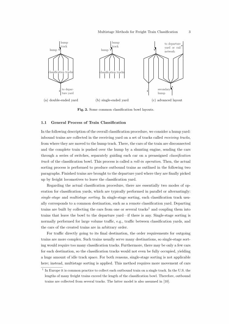
Multistage Methods for Freight Train Classification 3
humptrack
hump
to depar-ture yard
classification tracks
(a) double-ended yard
humptrack
hump
classification tracks
(b) single-ended yard
secondaryhump
to departureyard or railnetwork
(c) advanced layout
Fig. 2. Some common classification bowl layouts.
1.1 General Process of Train Classification
In the following description of the overall classification procedure, we consider a hump yard:
inbound trains are collected in the receiving yard on a set of tracks called receiving tracks,
from where they are moved to the hump track. There, the cars of the train are disconnected
and the complete train is pushed over the hump by a shunting engine, sending the cars
through a series of switches, separately guiding each car on a preassigned classification
track of the classification bowl. This process is called a roll-in operation. Then, the actual
sorting process is performed to produce outbound trains as outlined in the following two
paragraphs. Finished trains are brought to the departure yard where they are finally picked
up by freight locomotives to leave the classification yard.
Regarding the actual classification procedure, there are essentially two modes of op-
eration for classification yards, which are typically performed in parallel or alternatingly:
single-stage and multistage sorting. In single-stage sorting, each classification track usu-
ally corresponds to a common destination, such as a remote classification yard. Departing
trains are built by collecting the cars from one or several tracks1 and coupling them into
trains that leave the bowl to the departure yard—if there is any. Single-stage sorting is
normally performed for large volume traffic, e.g., traffic between classification yards, and
the cars of the created trains are in arbitrary order.
For traffic directly going to its final destination, the order requirements for outgoing
trains are more complex. Such trains usually serve many destinations, so single-stage sort-
ing would require too many classification tracks. Furthermore, there may be only a few cars
for each destination, so the classification tracks would not even be fully occupied, yielding
a huge amount of idle track space. For both reasons, single-stage sorting is not applicable
here; instead, multistage sorting is applied. This method requires more movement of cars1 In Europe it is common practice to collect each outbound train on a single track. In the U.S. the
lengths of many freight trains exceed the length of the classification bowl. Therefore, outbound
trains are collected from several tracks. The latter model is also assumed in [10].
4 Riko Jacob, Peter Marton, Jens Maue, and Marc Nunkesser
but allows much more flexible and efficient use of the tracks than single-stage sorting. In
multistage sorting, after the incoming trains have been pushed over the hump (primary
sorting), a shunting engine repeatedly pulls back the cars from a given track (pull-out
operation) over the hump on the hump track. These cars are then pushed over the hump
again, so that again each car can be independently routed through the switches to any
classification track. This process is iterated until all outgoing trains have been formed.
This part of the sorting procedure is called secondary sorting. If a classification track is
used only for receiving cars of an outgoing train, but the cars on it are never pulled back
to the hump track, it is called train formation track.
1.2 Related Work
Multistage methods are presented from an engineering point of view in a number of pub-
lications from the 1950s and 1960s [2, 3, 13, 16, 21, 22, 25]. Krell [21, 22] compares the two
basic multistage methods sorting by train and the simultaneous method togwther with two
improvements of the latter, called triangular sorting and geometric sorting, respectively.
(We will describe these four important methods in further detail in Section 4 by means
of our representation of classification schedules introduced in Section 3.) Krell also in-
cludes an example showing how to deal with a restricted number of available classification
tracks, which anticipates our generalized method for this kind of restriction as introduced
in Section 5. Sorting by train and the simultaneous method had been described earlier in
a different fashion by Flandorffer [16] and by Pentinga [25]. Boot [3] describes the opera-
tional constraints when the simultaneous method was introduced in France, Belgium, and
The Netherlands. Other practical considerations regarding its real-world implementation,
such as required yard layouts or arrival and departure times of freight trains, can be found
in [22] and [13].
Some of these methods were again considered by Siddiqee [26] in 1972 and in a series of
publications in the 1980s by Daganzo, Dowling, and Hall [6–9]. Siddiqee summarizes the
main characteristics of the four methods mentioned above with regard to their applicability
under different conditions [26]. The author recommends which method is suitable under
which circumstances, taking into account the number and length of the tracks, the number
and sorting requirements of outgoing trains, and the finishing times of the ougoing trains.
In [9] the triangular method is analyzed with regard to the differences when applied in
hump and flat yards. Triangular sorting and sorting by train are compared in a practical
example in [6] including the concept of treating several outgoing trains as one, which the
authors call convoy formation [6]. [7] and [8] introduce a variant of these two methods,
called dynamic blocking, which reduces the number of required tracks for homogeneous [7]
and heterogeneous traffic [8], respectively.
Baumann [2] explains the design aspects concerning multistage train formation for the
example of the classification yard Zurich-Limmattal in Switzerland. The resulting layout
Multistage Methods for Freight Train Classification 5
features a secondary hump similar to Figure 2(c), which is, however, currently not used
due to cost and organizational reasons [19].
For single-stage sorting, more theoretical research has been done than for multistage
sorting in the last decade. An algorithmic single-stage sorting problem was studied by
Dahlhaus et al. [10, 11]. For their train classification model, they give a notion of presort-
edness of the incoming train which is used to improve the classification process. Several
degrees of freedom in the order requirement of the outbound train are regarded in [11],
while finding an optimal schedule is shown to be NP-hard in [10] for the output require-
ment in which cars of the same type must appear consecutively but the order of types is
free.
A systematic framework for classifying single- and also multistage classification meth-
ods is given by Hansmann and Zimmermann [18]. For the case of a limited number of
classification tracks and an extended output requirement which handles several cars of the
same type, they independently obtain the result we give in Section 5. Furthermore, the
authors show for a specific multistage method that finding an optimal schedule is NP-hard
for the output specification of [10] mentioned above.
The four methods mentioned in the first paragraph of this section are still the most
widely applied multistage methods today, and they have been studied quite thoroughly in
the engineering literature. We reconsider these methods from a theoretical point of view
in Section 4, including a simpler description and more precise analysis.
1.3 Our Contribution
The main contribution of this paper is a novel encoding scheme for train classification
schedules. This scheme offers an efficient and consistent representation of classification
schedules, which we apply to analyze and prove certain properties of existing train clas-
sification methods. Secondly, we introduce the number of pull-out steps as an accurate
yet very simple cost function for classification schedules, while we still take account of the
traditional cost measure of bounding the number of roll-ins for every car as our secondary
objective. Together with our encoding and a notion of presortedness for incoming trains,
we obtain optimal schedules for sufficiently large yards, which implies in particular that it
is impossible to outperform these schedules on real, restricted yards. We derive schedules
for a restricted number of classification tracks. For tracks of limited length, we show the
problem is NP-hard, give a 2-approximation and an exact algorithm for a special case.
The main results are summarized in the following list:
– concise encoding of classification schedules (Section 3)
– provably tight lower bound for length of schedules (Theorem 2)
– application of novel encoding yielding a simpler, more precise analysis of well-known
multistage methods (Section 4)
– polynomial-time algortihm to produce optimal schedules for yards with a limited num-
ber of tracks (Section 5)
6 Riko Jacob, Peter Marton, Jens Maue, and Marc Nunkesser
– NP-hardness of general problem with tracks of bounded length (Section 6.1)
– polynomial-time 2-approximation for tracks of bounded length (Section 6.2)
– exact algorithm for tracks of bounded length if the incoming train is not assumed to
be presorted (Section 6.3)
1.4 Outline
In the following section we introduce the above described problem and concepts formally,
including our objective. In Section 3 we present our novel encoding for representing clas-
sification schedules, which allows us to concisely describe and analyze the above methods
in Section 4. We proceed with analyses of new problem variants in Section 5 (restricted
number of classification tracks) and Section 6 (tracks of restricted capacity). In Section 7
we briefly discuss secondary objectives and conclude with practical remarks and future
work in Section 8.
2 Model and Notation
In this section we introduce the terminology and notation used in our model. We assume
the common yard layout of a single- or double-ended classification bowl with a single hump
as shown in Figure 2(b) and Figure 2(a), where the classification tracks are denoted by
θ1, . . . , θW . We denote their number by W , the width of the yard. We further assume that
all tracks have the same length and denote by Cmax the capacity of the yard, i.e., the
maximum number of cars that fit on a track.
Any car τ will be represented by some positive integer τ ∈ N and a train T by an
(ordered) k-tuple T = (τ1, . . . , τk) of cars τi ∈ N, i = 1, . . . , k. Note that the engine,
depending on the situation, may be at either end of the train and is not included in
this definition. The number of cars k will also be called the length of T . In our model,
there is a set of ` incoming trains and m order specifications corresponding to m outgoing
trains, and our goal is to sort the incoming cars according to the given specifications to
obtain the outgoing trains. The sets of incoming and outgoing trains are together called
a classification task, for which we make the following assumptions: for the ` incoming
trains T k = (τk1 , . . . , τkn′
k), k = 1, . . . , `, where n′k denotes the length of the kth incoming
train and n :=∑`k=1 n
′k the total number of cars, we assume τkj ∈ {1, . . . , n} and that all
cars are distinct. Without loss of generality (w.l.o.g.), we assume that concatenating the
outgoing trains in their given order yields the sequence (1, . . . , n)—otherwise, the incoming
cars can be renamed; in other words, if nk denotes the length of the kth outgoing train,
k = 1, . . . ,m, the kth outgoing train is given by (1 +∑k−1i=1 ni, . . . ,
∑ki=1 ni). Hence, an
ordered set of m outgoing trains can be defined uniquely by an m-tuple n1, . . . , nm.
For any train T = (τ1, . . . , τk), car τ1 is called the head of T , and, for any pair of cars
τi, τj of T with i < j, we say τi is in front of τj . For a train T located on the hump track,
the head of T represents the car that is closest to the hump. For a train T located on some

Multistage Methods for Freight Train Classification 7
classification track, its head represents the car closest to the dead-end. Thus, the train in
Figure 3(b) is represented by (6, 1, 4, 2, 3, 5) and the train in Figure 3(j) by (1, 2, 3, 4, 5, 6).
Any multistage sorting method consists of a sequence of alternating roll-in and pull-out
steps. In order to specify a single pull-out step, it suffices to specify the classification track
from which to pull out all cars. Note that always all cars on a track are pulled out; still,
pulling only some cars can easily be achieved in this model by first pulling all cars and
directly rolling in some of them to the same track. To fully specify a roll-in operation,
however, a target track must be given for every car on the hump track. We call such a
pair of operations a sorting step or simply step. An initial roll-in followed by a sequence
of h sorting steps is called a classification schedule of length h. A classification schedule is
called valid for a classification task if it transforms the given set of incoming trains into
the set of outgoing trains. As mentioned before, our main objective will be the number of
sorting steps, while the traditional objective, the number of cars rolled in, is studied in
Section 7.
Definition 1 (Train Classification Problem). Given a classification task of ` incom-
ing trains T i = (τ i1, . . . , τin′
i), i = 1, . . . , `, and the lengths (n1, . . . , nm) of the m outgoing
trains, the train classification problem is the problem of finding a valid classification sched-
ule of minimum length. We call such a classification schedule optimal.
Note that, according to the definitions above, the term length may refer either to the
number of sorting steps of a schedule or to the number of cars of a train. In the remainder
of this paper, the respective meaning will always be clear from the context. Moreover, we
will sometimes abbreviate statements referring to pull-out steps, such as abbreviating “the
cars of a track are pulled out” to “a track is pulled (out)”.
3 Encoding Classification Schedules
In this section we introduce an encoding of classification schedules by sets of bitstrings.
Conversely, we show how to interpret such a set as a schedule, which yields a bijective
relation between sets of bitstrings and classification schedules. Furthermore, a notion of
presortedness is introduced for incoming trains, which allows one to deduce optimal sched-
ules. We first consider the case of sorting a single incoming train into a single outgoing train
in Section 3.1, which is extended to the general case in Section 3.2. Both sections assume
classification yards without any restrictions on the number or capacities of the classfication
tracks. (Restricted settings are considered in later sections.) This section concludes with
practical notions on our concept of presortedness in Section 3.3.
3.1 Single train
We start by introducing a simplified view of the tracks. After a track has been emptied,
cars may be sent to it in subsequent steps, so one physical track might be filled and

8 Riko Jacob, Peter Marton, Jens Maue, and Marc Nunkesser
emptied more than once during a classification procedure. We model this by introducing
logical tracks that we define such that pull-out i is performed on logical track i. This means
that the logical tracks are pulled out in the order (1, 2, . . . , h). For a classification schedule
of length h, the mapping from the h logical tracks to the W physical tracks is given by a
sequence (θi1 , . . . , θih) of physical track names, called the track sequence.
The course of a single car τ can now be represented by an h-bit binary string b = bh . . . b1,
bi ∈ {0, 1}, where bi = 1 if and only if τ visits the i-th (logical) track. (In the following,
these strings are interpreted as binary representations of non-negative integers with bh
being the most significant bit of b; in the usual depiction, this corresponds to using the
tracks from right to left.) This representation uniquely defines the course of car τ : τ is
pulled out in the i-th step if bi = 1 simply because it has been sent there in some earlier
step. Then, it is rolled in on the k-th track given by k := minj>i,bj=1 j, i.e., the lowest
bit bk = 1 left of i. If bj = 0 for all j > i, then τ is sent to the train formation track of
its target train. The track for the initial roll-in is given by the least significant bit bi with
bi = 1. The complete schedule for a train of n cars can now be represented by a binary
encoding of length h given by B = (b1, . . . , bn), a sequence of binary numbers (bitstrings),
such that bj = bjh . . . bj1 encodes the course of the jth car, j = 1, . . . , n. We will always
use superscripts to refer to the bitstring of a car, e.g., bj is the bitstring of the jth car of
some train. Subscripts will refer to a single bit of some bitstring, e.g., the ith bit of some
bitstring b is referred to by bi.
An example is given in Figure 3, which shows a classification procedure and the binary
representation of its schedule for a single incoming train of six cars. There are more
classification tracks than schedule steps, so the above mentioned mapping from logical to
physical tracks does not use any physical track more than once. Note that in our model
the classification process is not yet finished in situations (e) or (g); a valid outgoing train
is obtained only when the situation in (j) has been reached.
We will repeatedly use the following ordering of bitstrings in this section: let b =
bh−1 . . . b0 and b′ = b′h′−1 . . . b′0 be two bitstrings of lengths h and h′, respectively, and
let x =∑h−1i=0 2ibi and x′ =
∑h′−1i=0 2ib′i be the integers corresponding to these bitstrings.
Then, if x < x′, we say that b is smaller than b′, denoted by b < b′. In other words, we
order bitstrings by the order of the integers they represent.
The following lemma shows how to read the binary representation of schedules: if two
cars have different bitstrings, the car with the smaller bitstring will be located in the target
train at a position closer to the head of the train. If two cars have the same bitstring, they
will not swap their relative order.
Lemma 1. Let B = {b1, . . . , bn} be the binary encoding of a classification schedule for an
incoming train T = (τ1, . . . , τn). Two cars τi and τj, i < j, swap their relative position if
and only if bi > bj.
Proof. If bj < bi, let k be the most significant index with bjk = 0 and bik = 1. Car τi is
sent to some track θnext in sorting step k. As bj` = bi` for all ` > k, car τj was already sent
Multistage Methods for Freight Train Classification 9
1 0 0
0 1 0
0 0 1
0 1 1
0 0 0
1 0 1
4
2
5
3
1
3
0
5
2
4
1
6
τ6
τ5
τ4
τ3
τ2
τ1
(a)
5
3
2
4
1
6
θ1θ2θ3θ6
(b)
θ1θ2θ3θ6
1 5 3 6
4
2
2
4
1
3
5
6
(c)
θ1θ2θ3θ6
2
4
6351
2
4
6
(d)
θ1θ2θ3θ6
351
6 42
6
4
2
(e)
θ1θ2θ3θ6
6
5
4
3
2
1
4
3
(f)
θ1θ2θ3θ6
6
5
2
1
4
4
3
3
(g)
θ1θ2θ3θ6
1
2
3
4
6
5
6
5
(h)
θ1θ2θ3θ6
1
2
3
4
6
6
5
5
(i)
θ1θ2θ3θ6
6
5
4
3
2
1
(j)
Fig. 3. A classification procedure for h = 3 and n = 6, using track θ6 for the output train. The
encoding is shown in (a), the input train in (b). (c)–(j) show the consecutive situations during
the procedure, always pulling out the cars of the rightmost occupied track.
to θnext in a previous step, so τj appears at a position in front of τi on θnext. For the same
reason, the two cars will not swap their relative order at any step later than k, so τj ends
up on the output track at a position in front of τi in the outgoing train.
Conversely, if bj > bi, swapping the roles of bi and bj in the above argument yields
that τi ends up in the outgoing train at a position in front of τi, so their order has not
swappped. Finally, if bi = bj the two cars will go exactly the same course and end up in
the same order as in T . 2
In the following theorem, we show that there is a bijection between valid classification
schedules and binary encodings with a special property.
Theorem 1. Let T = (τ1, . . . , τn) be an incoming train, and let B = (b1, . . . , bn) be the
binary encoding of a classification schedule with each bi being a bitstring of length h,
i = 1, . . . , n. In a classification yard of sufficient width and capacity, B represents a valid

10 Riko Jacob, Peter Marton, Jens Maue, and Marc Nunkesser
schedule of length h for T if and only if the following properties are both satisfied:
For all i, j ∈ {1, . . . , n} if i < j ∧ τi > τj then bi > bj . (P1)
If bi > bj then τi ≥ τj . (P2)
Proof. Property (P1) states that if two cars need to be swapped (i < j and τi > τj) they
are swapped, which follows from Lemma 1. If bi > bj car τj ends up in front of car τi,
irrespective of their prior order. This is correct if τi ≥ τj . Therefore, by property (P1) cars
that need to change their relative positions do so. Together, these two properties imply
the validity of the schedule. 2
As a consequence of the above theorem, an optimal schedule corresponds to a binary
encoding B of minimum length h that satisfies properties (P1) and (P2). To construct an
optimal schedule, we must take the shortest possible bitstrings, so we need to use as few
different bitstrings as possible. Therefore, we want to know which cars of the incoming
train can get the same bitstring, which leads to the following notion of presortedness.
Definition 2 (Chains). Given an incoming train T = (τ1, . . . , τn), a pair of cars τj , τkis called a break if j < k and τj = τk + 1; in other words, if two cars τj, τk appear
consecutively in the outgoing train but are in the wrong order in the incoming train, they
are called a break. The set of breaks of T uniquely decomposes each train into maximal
subsequences of cars in the correct order; such a subsequence is called a chain, and the set
of chains can be ordered ascendingly by their first elements.
For example, train T = (9, 4, 5, 7, 1, 2, 8, 6, 3) uniquely decomposes into the disjoint chains
c1 = (1, 2, 3), c2 = (4, 5, 6), c3 = (7, 8), and c4 = (9), which we call the chain decomposition
of T .
By Definition 2 all cars of a chain are in the correct relative order with respect to
the outgoing train, so, by Lemma 1, these cars can get the same bitstring. The following
lemma shows how to assign bitstrings to chains.
Lemma 2. Let T = (τ1, . . . , τn) be an incoming train and let B = (b1, . . . , bn) be a valid
schedule for T . If two cars τi < τj belong to different chains, then bi < bj.
Proof. If i > j, then τi and τj must swap their relative order since τi < τj , so bi < bj must
be satisfied by Lemma 1. If i < j, then there is a car τx with τi < τx < τj and either x < i
or x > j. (Otherwise, τi and τj would be in the same chain.) If x < i, then bi < bx and
bj ≥ bx by Lemma 1, so bi < bj . Similarly, if y > j, then bj > by and bi ≤ by by Lemma 1,
so bi < bj . 2
The above assignment of bitstrings to chains finally yields the main result of this
section, which is summarized in the following theorem.
Theorem 2 (optimal schedules). Let T = (τ1 . . . τn) be a train of length n and let c be
its number of chains. In a classification yard of sufficient width and capacity, the optimal
classification schedule B for T has length h = dlog2 ce.
Multistage Methods for Freight Train Classification 11
Proof. As shown above, in a valid schedule cars of the same chain can be assigned the same
bitstring. Hence, c bitstrings are sufficient for a valid assignment of bitstrings to cars, so
h ≤ dlog2 ce as there are 2h different bitstrings of length h. Conversely, by Lemma 2, cars
of different chains must be assigned different bitstrings. Thus, at least c different bitstrings
are required for a valid schedule, so the length of any valid schedule satisfies h ≥ dlog2 ce.2
This result can be extended to more complex objective functions as explained in Sec-
tion 7.
3.2 Multiple Trains
Any real-world classification task involves multiple incoming and multiple outgoing trains.
Once the order of the incoming trains has been determined, such a classification task can
be solved by separately solving, for each outgoing train, one classification task of a single
incoming and single outgoing train. The individual solutions can then just be appended,
which is shown in the following section. In the subsequent section, we deal with choosing
an optimal order of multiple incoming trains.
Multiple Outgoing Trains In the following theorem, the sequence of incoming trains
in a fixed order is regarded as a single incoming train.
Theorem 3. For a classification yard of unrestricted width and capacity, let T = (τ1, . . . , τn)
be an incoming train, and let m outgoing trains be given by their lengths (n1, . . . , nm).
Furthermore, let Ti be the subsequence of T corresponding to the ith outgoing train,
i = 1, . . . ,m, and let Bi be the optimal schedule for the task of sorting Ti into the ith
outgoing train, i = 1, . . . ,m. The length |B| of an optimal schedule B for the sorting task
given by T and (n1, . . . , nm) is |B| = max1≤i≤m
|Bi|.
Proof. Every outgoing train has a separate train formation track, so if two cars belong to
different chains with respect to different outgoing trains, their relative order is irrelevant
during the whole classification process. Hence, they can be assigned the same bitstring. In
the optimal schedule B, every car can thus be assigned to the bitstring it is assigned to in
its respective schedule Bi, artificially increasing the length of the bitstring to max1≤i≤m
|Bi|by adding leading zeros. 2
The theorem statement does not change for classification yards with a restricted number of
tracks as discussed in Section 5. For tracks of restricted capacity as discussed in Section 6,
however, the theorem does not hold.
Multiple Incoming Trains We have assumed a fixed order of the incoming trains so
far. This assumption is reasonable in most practical cases where the incoming trains arrive
distributed over time. Assuming a single outgoing train, changing the order of incoming
trains, however, may change the number of breaks in the resulting sequence of incoming
12 Riko Jacob, Peter Marton, Jens Maue, and Marc Nunkesser
cars. Hence, if the order can be chosen freely, the problem of choosing an optimal order of
incoming trains arises.
Definition 3. Given ` incoming trains Ti = (τ i1, . . . , τin′
i), i = 1, . . . , `, OPT-PERM is
defined as the problem of finding a permutation π that minimizes the number of breaks in
the concatenation Tπ(1) · · ·Tπ(`) of the incoming trains.
Below, Lemma 3 shows the problem OPT-PERM is equivalent to a special minimum
feedback arc set problem. The general minimum feedback arc set problem (MinFAS) is
defined in the following way: given a directed graph G = (V,E), find a linear arrangement
π(V ) of V that minimizes the number of edges (u, v) ∈ E with π(u) > π(v). Put less
formally, find an arrangement of nodes that minimizes the number of backward edges. A
detailed survey of feedback arc set problems can be found in [15].
For multiple incoming trains, breaks may occur between two cars of the same incoming
train (which we will call internal breaks) or between two cars of different incoming trains
(external breaks). This is summarized in the following definition which is used in the proof
of Lemma 3 below.
Definition 4. Let T = (T 1 · · ·T `) be the concatenation of ` incoming trains T i = (τ i1, . . . , τin′
i),
i = 1, . . . , `, and let p = (τ ix, τjy ), i, j ∈ {1, . . . , `}, be a break of T , i.e., τ ix = τ jy + 1 and
either i < j or i = j and x < y. If i < j, then p is called an external break between T i
and T j. If i = j, then p is called an internal break of T i.
The following lemma finally shows the equivalence between OPT-PERM and MinFAS in
a special class of graphs.
Lemma 3. There is a one-to-one correspondence between OPT-PERM and MinFAS for
directed multigraphs the edges of which form an Eulerian path.
Proof. We first show how to transform OPT-PERM from Definition 3 into a minimum
feedback arc set instance G = (V,E). Each incoming train T i is mapped to a node n(T i).
For each pair of cars τk ∈ Tα, τj = τk + 1 ∈ T β , we add a directed edge (n(Tα), n(T β))
to E. Traversing the sequence of cars in this way, we add exactly n− 1 edges, potentially
self-loops, to G, and these edges form an Eulerian path by the construction. We remove
the self-loops and still have an Eulerian path. If π is any permutation of incoming trains
and T denotes the resulting incoming sequence of cars, the number of external breaks of
T equals the number of arcs pointing backwards in the linear arrangement π(V ). Since
the number of internal breaks of T does not change by altering the order of incoming
trains, a permutation of trains minimizing the total number of breaks corresponds to an
arrangement of nodes that minimizes the number of backward arcs.
For the other direction, the following construction obviously transforms any multigraph
with an Eulerian path into an instance of OPT-PERM with the same relation of the
objective functions: for each node n ∈ V , we introduce an incoming train T (n). Then, we
walk along the Eulerian path P = (ni1 , . . . , nim) and add for each nij ∈ P a car j to train
T (nij ). 2

Multistage Methods for Freight Train Classification 13
To the best of our knowledge, the complexity status of MinFAS in such graphs is open.
By a lemma of Newman, Chen, and Lovasz [24, Theorem 4], however, a polynomial al-
gorithm for OPT-PERM would lead to a 169 -approximation algorithm for MinFAS in
general graphs, substantially improving over the currently best known O(log n log log n)-
approximation [14].
3.3 Groups and Blocks
Another important practical complication concerns groups and blocks that occur in real-
world classification. These concepts are closely connected to presortedness of incoming
trains, to sorting specifications of outgoing trains, and thus to our notion of chains. We
will see that these aspects do not significantly change the results above.
A group is a set of cars with the same destination, typically the same customer. These
cars can come from different incoming trains but always go to the same outgoing train,
where they occur consecutively. The order of cars in a group is irrelevant. Still, the order
of the groups in the outbound trains is fixed. A block is a set of cars (or groups) that take
a common itinerary over potentially many classification yards. A block is not broken up at
intermediate classification yards. The associated blocking and makeup problems are out
of the scope of this paper; see [1, 5] for references. Blocking is particularly advantageous
in large countries like the U.S. and usually not applied in European freight systems [4].
Both concepts are related in the following way: before a block starts its itinerary over
several yards, it must be built at some origin classification yard. If the block is to be built
by multistage sorting, it can be regarded as a group of an outgoing train and can be formed
in the same way. If a block arrives at an intermediate destination, it is not broken up and
can be regarded as a weighted car for the classification task. Finally, a block arriving at
the final destination yard of its itinerary is broken up like an incoming train and has no
influence on the classification schedule. Thus, for our purposes, both groups and blocks
lead to exactly the same complication: some cars must be sorted in a sequence the order
of which is irrelevant. Therefore, w.l.o.g., we will only refer to groups below.
To adapt our model we simply drop the constraint that all cars (τ1, . . . , τn) of a train
must be distinct. It is easy to check that with this definition Lemma 1 and Theorem 1
still hold. Theorem 1 applied to trains with groups, however, leads to a different notion of
chains than the one in Definition 2.
As an analogue of Definition 2 and Lemma 2 we redefine chain decompositions with
our goal of extracting optimal binary encodings from them:
Definition 5. Given a train T = (τ1, . . . , τn) with not necessarily distinct τi, a chain de-
composition Ξ = (c1, . . . , ck) is a partition of T into subsequences, such that the following
resulting classification schedule is valid: Only the binary representations of i−1, 1 ≤ i ≤ k,
are used. All cars of chain ci are assigned the binary code i− 1, and this binary encoding
is called B(Ξ). We call Ξ optimal if B(Ξ) is optimal.

14 Riko Jacob, Peter Marton, Jens Maue, and Marc Nunkesser
Observe that there is no longer a single optimal chain decomposition. For example, for
the train (3, 1, 4, 1, 2, 2, 3, 5, 4) both (1, 1, 2, 2), (3, 3, 4), (4, 5) and (1, 1, 2, 2, 3), (3, 4, 4), (5)
are optimal. The second chain decomposition in the example has been obtained in the
following greedy way: The first chain c1 contains all possible cars with τ· = 1. All cars
with τ· = 2 can get the same bitstring by Lemma 1. All occur after the last τ· = 1. They
are included in c1. Not all cars with τ· = 3 can get the same bitstring, because the first
3 needs to be swapped with the 1s and 2s. Still, the second 3 can get the bitstring of the
first chain because it does not need to be swapped with the 1s or the 2s. It follows that
(1, 1, 2, 2, 3) is the longest possible sequence of cars that can get the same bitstring and
contains the smallest car, here τ· = 1. The remaining chains can be obtained by iterating
this procedure on the remaining cars. Let us call the resulting chain decomposition the
greedy chain decomposition. We now show the analogue of Theorem 2 for groups.
Theorem 4. (greedy chain decomposition is optimal) Let T = (τ1, . . . , τn) be a train with
not necessarily distinct τi. The greedy chain decomposition Ξg = (c1, . . . , ck) of T leads to
an optimal classification schedule of length dlog2 ke encoded as B(Ξ) for a classification
yard of unrestricted width and capacity.
Proof. Assume for a contradiction that there is another chain decomposition with fewer
chains. We want to compare chains car by car and therefore distinguish the cars by in-
dices. The above example becomes (31, 11, 41, 12, 22, 23, 32, 5, 42). Select the optimal chain
decomposition Ξopt = (d1, . . . , dk′), with k′ < k that has the longest identical start se-
quence of chains (c1 = d1, c2 = d2, . . .) among all optimal chain decompositions. Again,
for the above example we have (11, 22) 6= (12, 22). Now consider the first pair of chains
(cx, dx), where Ξg and Ξopt differ. From the greedy construction and the fact that the two
decompositions agree up to cx and dx it follows that cx must be longer than dx. In fact,
dx ⊂ cx because all cars in dx can be included in cx independent of the cars in cx \ dx. We
modify Ξopt to Ξ ′opt by replacing dx by cx and removing the cars in cx \ dx from the rest
of the chains in Ξopt. Note that we cannot invalidate a chain by removing cars from it.
Now Ξ ′opt is a chain decomposition and agrees with Ξg on one more chain in contradiction
to the assumption. 2
4 Multistage Classification Methods
In this section we describe the multistage classification methods mentioned in Section 1.2
by means of the encoding introduced in Section 3. First, we explain how classification
methods can be regarded as classes of schedules. Then, sorting by train and the basic
version of simultaneous sorting are analyzed in Section 4.2, followed by two variants of the
latter called triangular and geometric sorting in Section 4.3.
Multistage Methods for Freight Train Classification 15
4.1 Classification Methods and Classes of Schedules
All schedules that follow a common classification method share common properties. For
the example of triangular sorting—an explanation of this method follows below—every
car is rolled in at most three times, so every schedule that accurately implements the tri-
angular method for some problem instance has this property. Every schedule can be repre-
sented by an encoding according to Section 3. Since this encoding contains the properties
of the schedule, it contains all properties of the classification method that the schedule
implements. Therefore, every classification method can simply be regarded as a class of
classification schedules with certain properties, so every classification method corresponds
to a class of encodings.
In the remainder of Section 4, we assume that we are given m outgoing trains by their
lengths n1, . . . , nm as explained in Section 2. Let g1, . . . , gm be the respective numbers of
groups in these trains. Define gmax = max1≤i≤m
gi and gmin = min1≤i≤m
gi.
4.2 Basic Multistage Methods
The multistage methods applied today can be categorized into two general classes: sorting
by train [6, 21, 26] and simultaneous sorting [16, 21, 25, 26], which have been extensively
described in the literature. Using our encoding, we achieve a more efficient description and
analysis of both methods in this section.
Sorting by Train Sorting by train comprises the following two stages. First, inbound
cars are separated according to their outgoing trains by sending all cars of a common
outgoing train to the same track. Second, the resulting unordered trains are processed
successively: a train is pulled back over the hump and rolled in again, sorting the cars
according to their groups by sending the cars of each group to the same track. Finally, the
groups of cars are moved from the tracks in the required order and coupled to form an
outgoing train. In double-ended yards this can be done from the opposite end of the yard.
The process continues with the next train. For the rest of this paper, the train formation
tracks will not appear in the encoding since they are implicitly given.
The corresponding class of encodings is given as follows: for the encoding bh . . . b1 of
any car in the `th group of the kth outgoing train, bi = 1 only for i = k +∑k−1j=1 gj
(corresponding to the initial roll-in) and i = k+∑k−1j=1 gj + ` (corresponding to the second
stage).
The length h of this schedule is given by h = m +∑mi=1 gi. This method occupies
exactly m classification tracks after the first stage, so the total number of tracks is at least
m+ gmin − 1, and at most m+ gmax − 1, while the latter number is tight if the first train
processed in the second stage has gmax groups.
Sorting by train is also called initial grouping according to outbound trains [26]. The
corresponding names used in the German literature are Ordnungsgruppenverfahren [21]
and Staffelverfahren.
16 Riko Jacob, Peter Marton, Jens Maue, and Marc Nunkesser
Simultaneous Sorting Unlike sorting by train, the first stage of the two-stage method
simultaneous sorting sorts according to the cars’ groups in the outgoing train. In the
encoding of a schedule of this class, this step forces bi = 1 for every car of the ith group
of any train. In the second stage, the cars are sorted according to their target trains:
the tracks are successively pulled out in the order of the corresponding group index, and
each set of cars pulled out is directly rolled back in, always sending cars of a common
outgoing train to the same train formation track. As mentioned before, this last roll-in is
not explicitly given in our encoding.
Simultaneous sorting minimizes the number of cars rolled in, which must be paid for by
a number gmax of sorting steps as there is one pull-out for every group, a number which is
maximal among all variants of simultaneous sorting for an unrestricted classification yard.
Regarding the track requirement, exactly gmax tracks are used in the first stage. Thus,
at most gmax + m − 1 tracks are needed since up to m − 1 further tracks are needed for
train formation, and at least gmin + m − 1 tracks are required: Even after renaming the
groups such that all outgoing trains have a group gmax and use the small numbers as little
as possible, pulling the first of the last gmin tracks to be pulled in the second stage forces
starting the formation of all m outgoing trains (if not yet started), so exactly gmin +m−1
tracks are occupied at this point.
In contrast to sorting by train, the formation of all outgoing trains is performed si-
multaneously, which explains the method’s name. Simultaneous sorting is also called the
simultaneous method, simultaneous marshalling [25], sorting by block [6], or initial group-
ing according to subscript [26]. The corresponding German terms are Simultanverfahren
and furthermore Elementarsystem to explicitly refer to the basic version described in this
section [21].
Note that in the above description cars are never guided to a train formation track
during primary sorting. This may be desired for operational reasons and is even necessary
if the train formation tracks cannot be accessed from the primary hump such as for a
layout as shown on the right of Figure 2(c). If the train formation tracks can be accessed
from the primary hump, however, the schedule becomes one step shorter.
4.3 Variants of Simultaneous Sorting
In the basic form of simultaneous sorting, every car is pulled out once and rolled in twice,
once in either stage. For the following variants this restriction is dropped. Instead of stages,
these variants are specified by sequences of sorting steps.
Triangular Sorting Triangular sorting has been considered in [6, 9, 16, 21, 25, 26]. This
method is a superclass of simultaneous sorting that is given by allowing at most three
roll-in operations for each car (including the final roll-in of a car to its outgoing train). For
the schedule encoding, this yields a restriction of bi = 1 for at most two indices i = 1, . . . , h
in the bitstring of every car.

Multistage Methods for Freight Train Classification 17
For this method Krell [21] gives an upper bound of 12h(h+1) on the maximum number
of groups gmax of an outgoing train that can be sorted in h steps. This result can be
reformulated in terms of chains yielding a better bound in general. If c1, . . . , cm denote
the respective numbers of chains of the trains and cmax = max1≤i≤m ci, for a sufficiently
large classification yard, classifying by triangular sorting can be done within h sorting steps
if cmax ≤ 12h(h + 1). This follows immediately by our encoding: the number of distinct
bitstrings bh . . . b1 of length h and bi = 1 for at most two different indices i ∈ {1, . . . , h} is
given by(h1
)+(h2
)=(h+1
2
), and the required number of distinct bitstrings is not greater
than the maximum number of chains by Lemma 2. Conversely, if some outgoing train has a
number of chains cmax, we must choose a set of cmax bitstrings with bi = 1 for at most two
different i ∈ {1, . . . , h}, which yields a feasible schedule of length h = d√2cmax − 12e that
can be applied in a sufficiently large classification yard. The method can be generalized
to any restriction on the number of roll-ins for a car.
The triangular-like occupation of the classification tracks after the initial roll-in ac-
counts for the name of this variant. In [21], triangular sorting is called Vorwartssortierung
bei hochstens zweimaligem Ablauf.
Geometric Sorting The method of geometric sorting [16, 21, 25, 26] is derived from
simultaneous sorting by dropping the restriction on the number of roll-ins completely,
which corresponds to bitstrings with no restriction at all. The performance of this method
is given in the literature by gmax ≤ 2h − 1 for h sorting steps [21]. Note that this number
differs from 2h by one as cars are not allowed to be sent to the train formation track in
the initial roll-in (for some practical reason), which corresponds to disallowing the all-zero
bitstring in our encoding. In combination with our notion of chains this exactly yields the
class of schedules of Theorem 2 with a bound of cmax ≤ 2h − 1, where cmax denotes the
maximum number of chains in any outgoing train.
Considering the special case of a single outgoing train of 2k−1 groups for some integer
k > 0, the initial roll-in sends 2k − i groups to the ith track, i = 1, . . . , k; the sum of these
numbers gives the geometric sum, which explains the method’s name. Geometric sorting
is called maximale Vorwartssortierung in [21].
As mentioned before, geometric sorting minimizes the number of sorting steps, assum-
ing the number and capacities of tracks are sufficiently large. If this cannot be assumed,
the simultaneous sorting variants of the following sections should be considered.
5 Restricted Number of Classification Tracks
In this section we consider schedules for classification yards with a restricted number W
of classification tracks. In Section 3 we derived schedules of length h = dlog2 ce for a
single incoming train with c chains. These schedules generally require one classification
track for every sorting step, i.e., W ≥ dlog2 ce must hold. (Note that the train formation
track is not included in the number W .) However, such a schedule is not valid in general
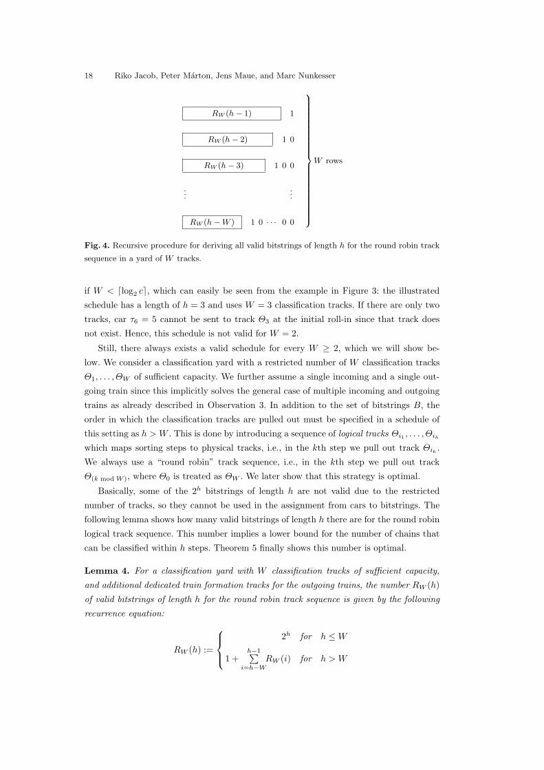
18 Riko Jacob, Peter Marton, Jens Maue, and Marc Nunkesser
RW (h− 1) 1
RW (h− 2) 1 0
RW (h− 3) 1 0 0
......
RW (h−W ) 1 0 · · · 0 0
9>>>>>>>>>>>>>>>>>>>>>=>>>>>>>>>>>>>>>>>>>>>;
W rows
Fig. 4. Recursive procedure for deriving all valid bitstrings of length h for the round robin track
sequence in a yard of W tracks.
if W < dlog2 ce, which can easily be seen from the example in Figure 3: the illustrated
schedule has a length of h = 3 and uses W = 3 classification tracks. If there are only two
tracks, car τ6 = 5 cannot be sent to track Θ3 at the initial roll-in since that track does
not exist. Hence, this schedule is not valid for W = 2.
Still, there always exists a valid schedule for every W ≥ 2, which we will show be-
low. We consider a classification yard with a restricted number of W classification tracks
Θ1, . . . , ΘW of sufficient capacity. We further assume a single incoming and a single out-
going train since this implicitly solves the general case of multiple incoming and outgoing
trains as already described in Observation 3. In addition to the set of bitstrings B, the
order in which the classification tracks are pulled out must be specified in a schedule of
this setting as h > W . This is done by introducing a sequence of logical tracks Θi1 , . . . , Θihwhich maps sorting steps to physical tracks, i.e., in the kth step we pull out track Θik .
We always use a “round robin” track sequence, i.e., in the kth step we pull out track
Θ(k mod W ), where Θ0 is treated as ΘW . We later show that this strategy is optimal.
Basically, some of the 2h bitstrings of length h are not valid due to the restricted
number of tracks, so they cannot be used in the assignment from cars to bitstrings. The
following lemma shows how many valid bitstrings of length h there are for the round robin
logical track sequence. This number implies a lower bound for the number of chains that
can be classified within h steps. Theorem 5 finally shows this number is optimal.
Lemma 4. For a classification yard with W classification tracks of sufficient capacity,
and additional dedicated train formation tracks for the outgoing trains, the number RW (h)
of valid bitstrings of length h for the round robin track sequence is given by the following
recurrence equation:
RW (h) :=
2h for h ≤W
1 +h−1∑
i=h−WRW (i) for h > W

Multistage Methods for Freight Train Classification 19
Proof. Let b = bh−1 . . . b0 be a bitstring of length h. Whenever a car is rolled in, it must be
sent to one of the W physical tracks. In the kth pull-out step of the round robin strategy,
these tracks always correspond to the W next pull-out steps, i.e., to the W next logical
tracks Θik+1 , . . . , Θi+k+W . (The inital roll-in can be regarded as following the 0th pull-out
step.) Therefore, if bk−1 = 1, bk−1+i = 1 must hold for at least one bit i = 1, . . . ,W ; in
other words, for b to be valid, there must not be a sequence of W consecutive bits all equal
to zero. However, since a car can always be sent to the train formation track, a leading
sequence of W or more zeros is still allowed. If h ≤W , a non-leading sequence of W zeros
cannot occur, so RW (h) = 2h in this case.
For longer bitstrings consider Figure 4: at the initial roll-in there are W choices for any
car, so bi = 1 must hold for some i = 0, . . . ,W − 1. Now, let i be the smallest such index
in b, corresponding to one of the W rows in Figure 4. After the pull-out corresponding to
bi = 1, there are again W choices of logical tracks to which to send a car assigned to b.
Additionally, there is the possibility to send the car directly to the dedicated track for the
outgoing train. The number of bitstrings starting with bi . . . b0 = 10 . . . 0 is RW (h− i− 1)
for this value of i. Summing over all W initial such sequences, corresponding to the rows
in Figure 4, we obtain RW (h) = 1 +∑h−1i=h−W RW (i). 2
The variation of the problem without dedicated tracks for the outgoing track has a
similar solution. The only difference is that leading zeros are forbidden as well, which
changes the recursion slightly:
Lemma 5. For a classification yard with W classification tracks of sufficient capacity,
where the outgoing train must be formed on the classification tracks, the number RW (h)
of valid bitstrings of length h for the round robin track sequence is given by the following
recurrence equation:
RW (h) :=
2h for h < W
h−1∑i=h−W
RW (i) for h ≥W
Note that in this case the number RW (h) is a generalization of the Fibonacci numbers.
In particular, for W = 2, we get R2(h) = Fh+2 where Fh is the hth Fibonacci number.
The proof of Lemma 4 yields a recursive procedure to derive optimal schedules, which is
applied in the following theorem.
Theorem 5. Given a classification yard with W classification tracks of sufficient capacity,
an incoming train with c chains can be classified within h steps if and only if c ≤ RW (h).
The corresponding classification schedule can be constructed in linear time (in the size of
the schedule).
Proof. The forward implication of the first statement immediately follows from Lemma 4.
For the reverse implication, we show round robin is optimal by induction. For the base
case of h ≤ W , the statement obviously holds. Now, assume the maximum number of
20 Riko Jacob, Peter Marton, Jens Maue, and Marc Nunkesser
bitstrings of length h (for the best possible track sequence) is RW (h′) for all h′ < h. Take
an optimal track sequence and set of bitstrings of length h. These bitstrings can be divided
into at most W classes by their second occurrence of a 1 (the positions depend on the
track sequence). If the classes are ordered according to this position, the first class contains
bitstrings of length at most h− 1, the second of length at most h− 2, and so on. Hence,
the number of bitstrings in the classes is bounded by RW (h− 1), RW (h− 2), and so on.
(This holds even if the different classes were allowed to have different track sequences.)
Therefore, at most RW (h) bitstrings are possible. Hence, the round robin logical track
sequence is optimal and no more than RW (h) chains can classified within h steps.
The proof of Lemma 4 yields a recursive procedure to construct a maximal set of valid
bitstrings of length h in time linear in the size of the set. The procedure can be applied
just partially in order to obtain an ordered set of c bitstrings of length h that present the
schedule in time linear in the size of the schedule. 2
As mentioned before, Hansmann and Zimmermann independently obtain the same
result in [18]. Moreover, a detailed example for this setting is already given in [21], though
the description is quite cumbersome as there is no efficient representation of classification
schedules. From the example, the maximum number of cars that can be sorted for a number
of given tracks is correctly deduced, but no proof is given.
6 Restricted Track Capacities
In Section 3 we derived optimal schedules for the simplified case of classification tracks
of unrestricted length. Real-world classification yards clearly have tracks whose length is
bounded. With this additional constraint, the problem of finding an optimal classification
schedule is NP-hard, which is shown in Section 6.1. For the same setting, we derive a factor-
two approximation algorithm in Section 6.2. In the special case that no assumptions about
the order of the cars in the incoming train is justified, an exact polynomial-time algorithm
is given in Section 6.3.
6.1 General Case
As mentioned above, assuming bounded track capacities for the classification tracks yields
an NP-hard problem. The bound on the track capacities is formalized as follows: All tracks
have a bounded capacity of C, i.e., they can accommodate at most C cars. This capacity
constraint is summarized in the following equation, where n is the number of cars, h the
length of the schedule, and bji denotes the i-th bit of the bitstring of the j-th car:
n∑j=1
bji ≤ C, i = 0, . . . , h− 1. (1)
The constraint does not apply to the train formation tracks, from which we furthermore
do not allow any pull-outs.

Multistage Methods for Freight Train Classification 21
Multiple Outgoing Trains The following theorem shows that the problem variant with
multiple outgoing trains and an unrestricted number of classification tracks with restricted
capacities is NP-hard. As a consequence, the train classification problem is NP-hard in its
most general variant.
Theorem 6. For a classification yard with classification tracks of restricted capacities,
finding the optimal classification schedule for a single incoming and multiple outgoing
trains is an NP-hard problem.
Proof. By reduction from the NP complete problem “Not ALL Equal 3-SAT” (NAE3SAT)
[17, LO3]. The input of NAE3SAT consists of n variables and m clauses, each of length 3.
The problem is to decide whether there is a truth assignment such that each clause has
at least one true and at least one false literal. Given an instance of NAE3SAT, we first
construct an instance of 2n incoming trains that are to be sorted into 2n outgoing trains
without any interaction between the trains, i.e., the ith incoming train has cars only for
the ith outgoing train. Note that even though there are multiple incoming trains their
order is irrelevant, because there is a one-to-one correspondence of incoming to outgoing
trains (this is in contrast to the general situation discussed in Lemma 3). For this reason
the incoming trains can be concatenated in any order into a single incoming train. For
ease of exposition, we start the proof by making two assumptions, and show later that
these can be easily enforced. First, each car can be part of at most one additional roll-in.
Second, we can have individual capacity bounds for all logical tracks.
The main idea of the proof is to allow a given number M = 4n+ 2m of steps and thus
logical tracks and to let all incoming trains have exactly M − 1 chains. Observe that if
two chains of the same train end up on the same track they must be in the wrong order,
which necessitates an additional roll-in incontradiction to the first assumption. It follows
that at most one of the chains of each train can be split or a single logical track can be
left unused. The transformation enforces the latter possibility for all trains.
From this construction it follows that the “local decisions” we can encode are for each
train, which track should be left unused. With the help of additional start and end gadgets,
the transformation forces the trains to have this unused track on the first or last logical
track, which encodes true and false. These true and false settings for the variables are used
in a middle part of the logical tracks that represents the clauses. In this part, the capacity
restriction on the tracks leads to the not all equal constraint on the clauses.
We proceed to show how to use this idea in the transformation and give an example in
Figure 5. First, for the incoming trains it is enough4 to specify the length of each of their
chains, instead of giving the full sequence that leads to these chains. For example we will
define a train as [1, 4, 2] by its sequence of chains (chain sequence) and ignore whether
this comes from an incoming train (2, 6, 1, 3, 4, 7, 5) or (6, 2, 3, 1, 4, 5, 7). Chains and logical
tracks are tightly connected because cars are pulled only once. For example, if there is4 All chain lengths will be polynomial in n and m. Therefore, this is only a matter of convenience
and does not change the result for a car by car input encoding.

22 Riko Jacob, Peter Marton, Jens Maue, and Marc Nunkesser
precisely one chain more than there are tracks, the first chain goes directly to the output
track, the second on logical track one, and so forth. By the convention of numbering logical
tracks from right to left (because of the relation to binary numbers), it is convenient to
reverse the order in the chain sequence and to omit the first chain that is rolled-in directly.
Hence, we write a compact chain sequence as 〈2, 5, 3〉 to mean the chain sequence [1, 3, 5, 2]
and an incoming train like (10, 11, 5, 6, 7, 8, 9, 2, 3, 4, 1).
(x1 ∨ x2 ∨ x3) ∧ (x1 ∨ x2 ∨ x3)
x1 x1 x2 x2 x3 x3 C+1 C−1 C+
2 C−2 x1 x1 x2 x2 x3 x3
x1 k 1 1 1 1 1 k 1 1 1 k 1 1 1 1
x1 k 1 1 1 1 1 1 1 k 1 k 1 1 1 1
x2 1 1 k 1 1 1 1 1 k 1 1 1 k 1 1
x2 1 1 k 1 1 1 k 1 1 1 1 1 k 1 1
x3 1 1 1 1 k 1 k 1 1 1 1 1 1 1 k
x3 1 1 1 1 k 1 1 1 k 1 1 1 1 1 k
Fig. 5. Sketch of the transformation for an example with two clauses on three variables.
Each compact chain sequence has 4n + 2m − 1 chains, which correspond to a start
variable part of length 2n, followed by a clause part of length 2m and an end variable part
of length 2n− 1. There are 2n chain sequences, one for each literal. All chains have either
length k (ON ) or length 1 (OFF ). The purpose of the start and end part of the chain
sequences is to force the gap into these parts. This is achieved by defining the start and
end parts of both xi and xi as follows:
〈start part︷ ︸︸ ︷
1, 1︸︷︷︸one pair/variable
, . . . , k, 1︸︷︷︸pair i
, 1, 1, . . .,
clause part︷︸︸︷. . . ,
end part︷ ︸︸ ︷1, 1, . . . , k, 1︸︷︷︸
pair i
, 1, 1, . . . , 1, 1〉
Both sequences have length M − 1 together with the clause part that remains to be
specified.
The first 2n logical tracks and the last 2n logical tracks have all capacity 2n + k − 1,
except for the first and the last track which have both capacity n+k−1. The total capacity
of the first 2n positions of all chain sequences exceeds the total available capacity for the
start part by n, and the same holds for the end part. This situation forces at least n gaps
in the start part and at least n gaps in the end part, thus exactly n gaps in both parts.
Having these identical subsequences for a variable and its negation enforces, together with
the capacity bound, that for each variable either there is a gap in the start part of the
chain sequence for xi and in the end part of the one for xi or vice versa. Thus, we can
think of the chain sequences for variable xi as either being left (xi = TRUE) or right
(xi = FALSE).
The clause part has 2m logical tracks, 2 for each clause. Precisely the trains corre-
sponding to literals occurring in this clause have a position in the chain sequence turned
Multistage Methods for Freight Train Classification 23
on, namely in a way that the chain is placed on one of the two tracks. The first track of
clause j stands for a literal making this clause true (contributing to set C+j ), the second
for one making it false (contributing to set C−j ). From above it follows that there can be
no gaps in the clause parts. We indicate the occurrences of literals in clauses by turning on
the corresponding position in the chain sequence, as exemplified in Figure 5. The chains
for each literal can be either left or right and therefore contribute either to C+j or C−j for
each clause j. By setting the capacity constraint to 2n + 2k − 2 for each logical track in
the clause part we enforce the not all equal constraint. This follows because this capacity
limit is exceeded if and only if three literals contribute to the same of the sets C+j and
C−j . Therefore, under the assumptions above the transformed instance is a yes-instance for
NAE3SAT if and only if there is a classification schedule that respects the given capacity
bound.
It remains to specify how to enforce the two assumed properties. First, we want to
replace the individual capacity constraints by a uniform one. To this end, we add one
chain sequence of full length M . As every car is only allowed to be pulled once, the
classification schedule for this chain sequence is unique. By adjusting the lengths of the
chains of this chain sequence, the differences in the capacity constraints can be adjusted.
To enforce that every car is pulled at most once, we add one chain sequence with one
chain of length 1 and one long chain. The length of the latter chain is exactly the excess
capacity of the logical tracks w.r.t. all chain sequences constructed before. Now, if any car
were pulled twice another car could not be pulled at all, which is impossible in a correct
classification schedule. 2
Single Outgoing Train The considerations so far depend on multiple outgoing trains.
Here, we show the complexity result holds even for a single outgoing train.
Theorem 7. For a single incoming and single outgoing train, with tracks of bounded
capacity, the problem of finding an optimal classification schedule is NP-hard.
Proof. We reduce the problem with multiple outgoing trains to this one. Let T1, . . . , Tk
denote the compact chain sequences of the k outgoing trains, and denote by |Ti| the total
number of cars in train i, not counting the first chain of length one that is not pulled
because it goes directly to the outgoing train. Let h be the limit on the number of sorting
steps, and C the capacity limit. Further, assume∑i |Ti| = h · C so that the cars must be
pulled exactly once. This is the kind of instance described in the proof of Theorem 6.
We define an instance with a single outgoing train where the original cars are pulled
precisely twice and there are additional long chains that are pulled precisely once. Let M =
max |Ti| + 1 so that all original chains are smaller than M . Define the new capacity to
be D = 2M and the new number of logical tracks H = k+ h. Define further di = D− |Ti|and e = D − C, and observe that di > M and e > M . Now, the single outgoing train has
24 Riko Jacob, Peter Marton, Jens Maue, and Marc Nunkesser
the compact chain sequence
T = 〈T1, d1, T2, d2, . . . , Tk, dk, e, . . . , e︸ ︷︷ ︸×h
〉
The enforced utilization of the tracks is schematically depicted in Figure 6.
Space for original codes
h
C
k
e
T3
hC
D
H
d3
Fig. 6. Track utilization scheme for the transformation into a single outgoing train.
It remains to show that T can be sorted in H steps on a capacity D yard if and only
if the Ti can be sorted simultaneously in h steps on a capacity C yard. Assume the latter,
and let Bi be the bitstrings for train i (having a single 1 by assumption). We precede
the bitstrings of Bi by 0s, only at position i we place a one. Further, the first chain gets
bitstring 0, the chain di the bitstring with a single 1 at position i, and the chains of length e
get the remaining bitstrings with a single 1, namely at positions k + 1, . . . ,H. This set of
bitstrings gives the correct order and uses capacity D on every position: On the first k
positions because of di + |Ti| = D, and on the remaining positions because the original
bitstrings used precisely capacity C. Hence, the train T can be sorted as claimed.
Now, conversely, assume that T can be sorted. Because di > M and e > M , the minimal
number of ones (car pulls) is given by a set of bitstrings that uses singleton bitstrings for
the di and e chains and bitstrings with two 1s for the chains of the Ti. Such a set of
bitstrings uses precisely D · H ones, and hence every correct set of bitstrings must have
this structure. Because of the ordering of T , the bitstring of di must have the 1 at position i
and the bitstrings of Ti must have their first 1 at position i. The singleton bitstrings for
the e chains leave precisely a capacity C on the h tracks k+1, . . . ,H. Hence, the second 1s
of the bitstrings for the Ti can be interpreted as bitstrings for the multiple train instance
because they are all in the last h positions. They meet the length and capacity requirement
and achieve the required ordering because the set of bitstrings was correct for the single
train instance. 2

Multistage Methods for Freight Train Classification 25
6.2 Approximation
In the previous section the train classification problem with restricted track capacities has
been shown to be NP-hard. In the following a 2-approximation is derived, which basically
consists of two consecutive steps: the procedure starts with a schedule not necessarily
satisfying the capacity constraints (1) but the relaxed constraint (2) given below. This
schedule is derived according to the proof of Lemma 6. Secondly, in this schedule every
column violating (1) is distributed over several newly introduced columns which meet the
capacity constraint as shown in Theorem 8 and Figure 7.
Consider the following constraint on the number of cars rolled in by a schedule B of
length h, i.e., on the number of bits bji in B with bji = 1:
h∑i=1
n∑j=1
bji ≤ Ch (2)
Every schedule B of length h that satisfies (1) also satisfies (2), whereas the converse
implication does not hold in general.
Lemma 6. Given a train T of length n, a minimum-length schedule satisfying (2) can be
obtained in polynomial time in the size of the schedule encoding.
Proof. Observe that there is no loss of generality in assuming that the schedule uses the
same code for all cars of one chain: If this should not be the case for a chain, choose the
code in the chain with the fewest 1s and use it for all cars of the chain. This schedule is
still valid and does not use more roll-ins than the original one.
For a fixed number h, let Bh denote a valid schedule of length h that minimizes the
number of cars rolled in. As detailed below, Bh can be obtained in polynomial time by a
dynamic programming approach, which shows the statement of the lemma.
To describe the approach, it is useful to consider the following alternative descrip-
tion of a schedule: Double the code length and change a code bh . . . b1 into the code
bh1bh−11 . . . b11, i.e., on every other position there are only ones. The corresponding tracks,
so called virtual tracks, contain all cars of the train, and the ordering of the cars sum-
marizes the effect of the already performed shunting steps. More precisely, we see fewer
chains, for example with the complete binary code, every shunting steps reduces the num-
ber of chains by a factor of two. In general, the difference in the sequence achieved by
one shunting step is that some chains get united, namely consecutive pairs of chains. The
chain c′c′′ is created from the higher numbered chain c′′ that has a 1 and the chain c′ tat
has a 0 at the position. Because the set of cars of disjoint resulting chains are disjoint,
there is no interaction between creating c′ and c′′.
The dynamic program has a table of the form D(i, c), where c is any intermediate
chain, i.e., an interval of cars in the outgoing train, and D(i, c) gives the fewest possible
roll-ins to create c with i shunting steps (on the ith virtual track). Clearly, D(0, c) = 0
precisely for the original chains; for all other chains D(0, c′) = ∞. For i > 0, the above
26 Riko Jacob, Peter Marton, Jens Maue, and Marc Nunkesser
discussion justifies the formula
D(i, c) = minc′c′′=c
(D(i− 1, c′) +D(i− 1, c′′) + |c′′|)
In this formula, c′c′′ denotes the concatenation of c′ and c′′ and |c′′| the length of c′′, which
gives precisely the number of roll-ins necessary to place c′′ (with 1 at the position) behind
c′ (with 0 at the position). Note that we allow c′′ to be the empty chain, i.e., it does not
get more expensive to create a chain at a later stage.
The interesting entry of the table is D(h, 1 . . . n) which should be compared with the
constraint (2). The schedule can be reconstructed in the usual manner by keeping track
of the split that achieved the minimum. The validity and total number of roll-ins of the
schedule follows from the chains appearing on the virtual tracks as claimed by the dynamic
programming table.
A single entry D(i, c) can be calculated in time O(|c|), so the total running time for the
dynamic programming part of the algorithm is O(hn3) since the number of chains, i.e.,
the width of the table, is given by(n2
) ∈ O(n2). The reconstruction time for the schedule
B is linear in the size of B, which is O(hn). 2
Increasing the length of a valid schedule allows reducing the number of cars rolled in.
Thus, if B′ is the shortest valid schedule that satisfies (2) and h′ denotes its length, the
length h∗ of the optimal schedule B∗ meeting (1) satisfies h∗ ≥ h′. This fact will be used
in the following theorem which finally states the 2-approximation. Its proof directly yields
an iterative algorithm to derive the corresponding schedule.
bi bi−1
v1
v2
v3
vd
bi+1
(a)
d− 1
bi bi−1
v1
v2
v3
vd
bi+1
(b)
d− 1
bi bi−1
v1
v2
v3
vd
bi+1
(c)
Fig. 7. One iteration step of the approximation algorithm for bounded capacities, applied to a
column bi that violates the capacity constraints (1).
Theorem 8. For any instance of the train classification problem with restricted track
capacities that has an optimal solution of length h∗, a valid schedule of length of at most
2h∗ can be obtained in polynomial time.
Multistage Methods for Freight Train Classification 27
Proof. Let B be a schedule of minimum length h that is valid w.r.t. the unrestricted
problem and further satisfies (2). (B can be obtained according to Lemma 6.) This schedule
is transformed iteratively, performing one iteration step for every column of B that violates
(1). The steps can be performed in an arbitrary order. Figure 7 depicts a single iteration
step.
For any column vector bi of B, let the load `i of bi be defined by `i :=∑nj=1 b
ji . Now,
let bi be a column vector with `i > C. Define d := d `iC e and divide bi into d consecutive
subvectors v1, . . . , vd such that each vk with k < d has a load of exactly C and the load of
vd is at most C (Figure 7(a)). Then, shift all columns bj with j > i exactly d− 1 positions
to the left by inserting d − 1 additional all-zero columns (Figure 7(b)). Finally, every vk
is moved to the left by k− 1 positions, and the corresponding entries in bi are set to zero,
which finishes the iteration step (Figure 7(c)).
After each step, the respective fixed column satisfies (1), which also holds for every
newly introduced column, so the resulting schedule satisfies (1).
For every column in B, this procedure yields at most one “underfull” column (load
less than C), and the total number of “tight” columns (load equal to C) will not exceed
h, so the resulting length is at most 2h. Since h ≤ h∗, where h∗ denotes the length of an
optimal schedule satisfying (1), the resulting valid schedule has a length of at most 2h∗.
2
The algorithm of this section can easily extended to multiple outgoing trains S1, . . . , Sm:
in the proof of Lemma 6, one table must be maintained for each outgoing train Sk,
k = 1, . . . ,m. In each step i, one row D(i, ·) is constructed in each table, which is repeated
until∑mk=1D(h, Sk) ≤ hC after some step h. A single table entry is still derived only from
entries in the same table, and also the reconstruction can be done independently for every
train. Finally, the proof of Theroem 8 can be applied to the resulting schedule without
any changes, just as for a single outgoing train.
6.3 Chains of Unit Length
As shown in Section 6.1, the train classification problem with tracks of bounded length
is NP-hard. In the following, however, we show that, if all chains consist of single cars,
optimal schedules can be constructed efficiently (in the size of the resulting encoding).
These schedules also work for situations with longer chains, the schedules are just not
optimal any more. This corresponds to a planning situation where the ordering of the cars
in the incoming train is not known and the proposed schedule must work for any ordering
that the train actually has.
Once again, classification schedules that are valid for tracks of bounded capacity C
have binary encodings B that satisfy constraint (1). In other words, for every column the
total number of 1s is bounded by C.

28 Riko Jacob, Peter Marton, Jens Maue, and Marc Nunkesser
Algorithm to produce an optimal set of bitstrings Note that the maximal set of
bitstrings for h positions uses 2h−1 ones at each position. If this exceeds the capacity (track
length) only by one, we can omit the single bitstring that has a 1 in every position. In the
other extreme, if the capacity is one, the largest set of bitstrings consists of the h bitstrings
with a single 1. We analyze this situation more deeply in the following example. Assume
that for the given capacity c, one can use all bitstrings with a single 1 (singletons), all
bitstrings with two 1s (pairs), and as many bitstrings with three 1s (triples) as possible.
Assume this can be done in a way such that all but at most two positions are at the capacity
limit c, and the remaining (≤ 2) positions have c − 1 1s. Then, this set of bitstrings is
clearly optimal, since any other way of choosing this many bitstrings will use at least the
same number of 1s in total. Using all bitstrings with a certain number of 1s per bitstring
will use the same capacity on all tracks.
The following lemma and its constructive proof show how to produce optimal sets of
bitstrings for all capacities. In our example from above, let c be the capacity left after all
singletons and pairs are assigned. In the above example, we can choose i = 3, n = b c·h3 c in
the following lemma to complete the set of bitstrings. Note that the order of the positions
is arbitrary.
Lemma 7. Let h, n, i be positive integers with h ≥ i, and n ≤ (hi). Then, there is a set
of n bitstrings of length h with precisely i 1s in each bitstring, such that the total number
of 1s at two positions differs by at most one. That is, there are numbers←−h +
−→h = h and
c = dnih e such that in←−h positions the total number of 1s is c, and in
−→h positions the total
number of 1s is c− 1.
Proof. The proof is by induction on h. The base case is h = i. Then n ≤ (hi) yields n = 1.
Now the bitstring consisting of i = h 1s (and no 0s) shows the statement of the lemma.
Now assume h > i and inductively assume that the lemma holds for all i and all h′ < h.
In one inductive step a set S1 of c bitstrings with 1s in the first position is created. In
the example of Figure 8, S1 = {a, b, c, d}. The remaining (i − 1)|S1| 1s of the bitstrings
in S1 are equally distributed over all remaining positions by an inductive application of the
lemma. In the example, this is the pseudo-box in the lower right corner. Again inductively,
the remaining bitstrings S2 have a 0 in the first position; in the example S2 = {e, f, g, h}.Because the positions are arbitrary, we can arrange the inductive results in a way that
distributes the used capacity evenly. More precisely, we can assume that the bitstrings
for S1 have all higher capacity positions to the right, whereas the bitstrings for S2 have
the higher capacity positions to the left. Now all positions but a middle segment have the
same capacity (one higher plus one lower). The middle segment deviates from this capacity
by at most one.
To complete the proof of the lemma, we only have to show that for both inductive
applications the two assumed inequalities are met. We define some abbreviations with
the following naming conventions: Subscripted values are associated with the respective
invocation of the lemma. Hence, the first invocation of the lemma is with h1 = h − 1 as

Multistage Methods for Freight Train Classification 29
a
b
c
d ab
b
a
c c
d d
e
f
g
e
f feg
gh h h
Fig. 8. Illustration of the recursive bitstring generation with three 1s per bitstring, 6 tracks of
length 4, yielding 8 bitstrings. The recursion uses all remaining 1s of a position (the vertical box),
and recursively adds the remaining positions of the bitstrings (the flat pseudo-box). Importantly,
the flat pseudo-boxes are chosen in a way that the remaining space is almost equal in the different
positions.
the bitstring length, i1 = i − 1 the number of 1s per bitstring, and n1 = c the number
of bitstrings, resulting in S1, where the positions with more 1s are higher numbered (to
the right). We invoke it another time with h2 = h − 1 as the bitstring length, i2 = i 1s
per bitstring, and n2 = n − c bitstrings, resulting in the set of bitstrings S2, where the
positions with more 1s are lower numbered (to the left).
Here h1 ≥ i1 and h2 ≥ i2 hold because we are not in the base case. To show the
inequalities involving the binomial coefficient, it is convenient to combine the two “fill-
heights” (or deviation from the maximal possible fill height), c and c−1, into an averaged
value c = nih . We mark all such average values by a hat. The average height resulting
from S1 on the remaining positions is necessarily c1 = c(i− 1)/(h− 1).
The bound on n implies c ≤ (h−1i−1
)(an alternative way to describe the assumption of
the lemma) because ni ≤ i · (hi) = hi · i ·
(h−1i−1
)which yields c = ni
h ≤(h−1i−1
). This gives the
required n1 = c ≤ (h−1i−1
)by integrality of the binomial coefficient. Hence, the assumptions
for the first recursive invocation of the lemma are met.
Now, let us define e =(h−1i−1
)−c, the deviation from the maximal possible capacity. For
the recursive applications of the lemma we are only interested in the last h− 1 positions.
We define the average total height for both recursive applications for these positions only:
c1+2 =←−h−1h c +
−→hh (c − 1) = ni−c
h−1 ≤ c, and the corresponding e1+2 =(h−1i−1
) − c1+2.
Observe that e ≤ e1+2(≤ e + 1). For the second invocation of the lemma we should
check c2 ≤(h2−1i2−1
)=(h−2i−1
), where c2 = c1+2 − c1. Observe h−1
i−1 c1 = c =(h−1i−1
) − e
such that we can express c1 = i−1h−1
(h−1i−1
) − i−1h−1e =
(h−2i−2
) − i−1h−1e. So, c2 = c1+2 − c1 =(
h−1i−1
) − e1+2 −(h−2i−2
)+ i−1
h−1e =(h−2i−1
)+ i−1
h−1e − e1+2 ≤(h−2i−1
), where the last inequality
relies upon h ≥ i making the coefficient of e smaller than one, hence the statement follows
by the already observed e ≤ e1+2. 2

30 Riko Jacob, Peter Marton, Jens Maue, and Marc Nunkesser
The recursive procedure implied by the proof of Lemma 7 is efficient: The initial task
of using h · i 1s in bitstrings is split into two subtasks. Hence, the number of leaves in the
recursion tree is O(h · i), and the total running time is polynomial.
Theorem 9. For positive integers h and C a set B of bitstrings of length h that obey
capacity constraint (1) of maximal cardinality can be constructed in time polynomial in |B|.
Proof. For some i, it is possible to use all bitstrings of length h with precisely j 1s for
j = 1, . . . , i− 1. The remaining bitstrings are constructed according to Lemma 7 (actually
its constructive proof) by taking the largest n (binary search) for which the resulting set
of bitstrings leaves at most i− 1 positions at capacity C − 1, and all other positions with
capacity C. The binary search can be avoided by formulating two procedures, one that
takes a parameter n, and another one that produces as many bitstrings as possible given
the constraints. 2
7 Secondary Objectives
The quality of a classification schedule is mainly determined by the time it takes to execute
the complete schedule. So far, we have estimated this time by the number of required
sorting steps. On the other hand, it is also practice to consider the total number of cars
rolled in as the main objective. (At some classification yards, this objective is used for
pricing classification requests of customers.) Clearly, both objectives contribute to the
total required time, and, in [23], their relation is summarized as follows: if the constants
cpull, croll, and cpush denote the time required for pulling out one track, the time the last car
needs to roll from the hump to a track, and the time for decoupling and pushing one car,
respectively, then a classification process of h steps and a total of r cars rolled in roughly
requires a time of h(cpull + croll) + rcpush. As mentioned before, the term h(cpull + croll)
dominates rcpush, hence the choice of h as our primary objective. A detailed example
supporting this idea with actual numbers for the constants and experimental results for h
and r is also given in [23].
Still, the total number of cars that are pushed over the hump and rolled into the
classification tracks also influences the total execution time. This secondary objective, the
number of roll-ins, equals the number of 1’s in an encoding. It can be incorporated into
the objective function in various ways. First, one could ask for the optimal solution with
respect to sorting steps that minimizes the number r of car roll-ins. We call such a solution
a slim h-optimal solution. A more general approach is to charge a cost of α for a pull-out of
a train (e.g., α = cpull +croll from above) and β for a roll-in of a single car (e.g., β = cpush).
We call a solution that is optimal w.r.t. this objective (h, r)-optimal. In the following, we
briefly discuss the consequences of the two new objective functions.
Until now we could safely assume without loss of generality that in each step a complete
track is pulled out. This situation is also common practice in real-world classification
yards. The following lemma shows that, in case of unrestricted capacity and width, it is

Multistage Methods for Freight Train Classification 31
not advantageous to only partially pull-out a track, i.e., to leave some cars on the track
and to pull-out the rest.
Lemma 8 (partial pull-outs). If we assume an unbounded number of tracks in a model
with or without track capacity, there is both a slim h-optimal and a (h, r)-optimal solution
without partial pull-outs. For the case of bounded width W it can be necessary to use partial
pull-outs to get a solution that is slim h- or (h, r)-optimal.
Proof. For the first statement, observe that any solution in which a track is partially
pulled out can be transformed into a solution on one more track in which the two parts
are rolled into different tracks. For the second statement, consider an example with W = 2
and n = 4 and assume unit chain length for simplicity. From Section 5 we know that since
n is between the fourth and the fifth Fibonacci number any feasible encoding scheme needs
at least five bit bitstrings that start and end with a one. A solution with minimum number
of ones without leading and trailing ones is 010, 011, 101, 110. Without partial pull-outs
the cost of this solution is 7 plus the initial and final roll-in and cannot be improved. This
solution, however, can keep the chain of bitstring 101 in its track, as it is the bottommost
chain in the step where it is rolled into the same track again. Thus one roll-in can be
saved by a partial pull-out, the slim h-optimal solution must use pull-outs, analogously
for (h, r)-optimal solutions. 2
We already know that it is NP-hard to find the optimal classification schedule for
capacity-bounded tracks. Therefore, we cannot hope for a polynomial algorithm for the
new objectives in this case. The basic version of the problem remains polynomial, however,
as shown in the following lemma.
Lemma 9. A slim h-optimal solution can be computed in polynomial time for the case of
unbounded number of tracks and unbounded track capacity.
Proof. For a given incoming train we can compute all chain lengths. The remaining prob-
lem is to select n bitstrings from the 2dlogne candidate bitstrings that make the solution
slim. The best subset of the n bitstrings has a minimum scalar product of the vector of
chain lengths and the vector of number of ones in the selected bitstrings. This subset can
be found in the obvious way by a dynamic program5 that computes a table of numbers
C(i, j) that represent the minimum cost of a solution for the first i chains that uses the
first j bitstrings. 2
The partial pull-outs do not invalidate the encoding scheme. For a given encoding it
is possible to read off the number of roll-ins with partial pull-outs. This is stated in the
following observation that directly follows from Lemma 1.
5 Unlike stated in the conference version of this article [20], the set of bitstrings with the minimum
number of ones is not necessarily an optimal solution. This statement only holds for chains of
unit length.

32 Riko Jacob, Peter Marton, Jens Maue, and Marc Nunkesser
Observation 1 A car τj of bitstring c = X
pos i︷︸︸︷1 Y ∈ {0, 1}h in an encoding for train
T is the front element in step i if for all τk ∈ T \ τj of bitstring Xk1Y ′k it holds that
Y < Yk ∨ (Y = Yk ∧ j < k).
We have focussed on slim h-optimal solutions here. The extension to (h, r)-optimal
solutions is straightforward in the sense that one can always search through the possible
values for h with dlog ne ≤ h ≤ n.
8 Concluding Remarks
We have developed an efficient encoding of freight train classification schedules that allows
us to present, analyze, and develop train classification methods for real-world classification
yards. This surprisingly simple yet powerful encoding can be used to analyze the efficiency
of commonly used multistage methods. We proved the optimality of the simultaneous
variant geometric sorting in terms of sorting steps, considering presorted input.
Practical Considerations Dealing with single and multiple incoming and outgoing
trains, with yards of restricted capacity and number of tracks, and with presorted in-
put, the results of this paper cover the core of the sorting task at real-world classification
yards. We have shown that the constraint on the capacities leads to an algorithmically
more difficult problem than the constraint on the number of tracks. Fortunately, in prac-
tice, the number of classification tracks presents the more restrictive constraint in modern
classification yards.
Railway practitioners may notice that some aspects and exceptions of real-world clas-
sification tasks are not covered here. Many of these aspects, however, can be incorporated
in our encoding scheme by a simple restriction on the bitstrings in an encoding. In [23],
we present an integer programming approach for the train classification problem in which
we indeed incorporate the following three restrictions:
First, in many classification yards, multistage sorting is performed for local freight
trains while the rest of the traffic is sorted by single-stage sorting. Primary sorting (as the
first step of multistage sorting) and single-stage sorting are performed at the same time
here. Secondary sorting is usually started after all trains from single-stage sorting have
left the yard, so more tracks are available for secondary sorting. In [23], we incorporate
this requirement in a way similar to the considerations of Section 5.
Second, there are classification yards featuring two parallel humps, such as the yard
of Lausanne Triage considered in [23]. In this case, two independent multistage sorting
processes can be performed: each hump is assigned a (disjoint) fixed set of classification
tracks and a subset of the outgoing trains. Incoming cars are assigned to the humps
according to their outgoing train and remain in the system of that hump during all primary
and secondary sorting.
Multistage Methods for Freight Train Classification 33
Third, some outgoing trains may have to leave before the complete multistage process
finishes. As each sorting step roughly requires a constant amount of time, the required
departure times can be assigned to the sorting steps. Hence, for every car, the latest
possible step can be calculated after which this car must be on the train formation track.
This is the last restriction incorporated in [23], and further practical restrictions may be
possible to incorporate too.
Furthermore, there are yards with a secondary hump at their opposite ends like in
Figure 2(c). As secondary sorting can be performed via this hump without blocking the
primary hump, it can be started without retarding the single-stage sorting process. As
mentioned in Section 1, secondary humps are not always used due to cost and operational
reasons.
Future Work Some interesting questions arise in the interplay between primary and
secondary sorting. It is not always a priori clear which traffic should go into secondary
sorting. This decision depends on the available capacity of the classification yard, the
distribution of work between different classification yards, and on the connected routing
of blocks through a network of yards.
Furthermore, it would be interesting to apply some of the theoretical results of this
article to improve the actual classification procedures applied in real-world classification
yards. To this end, we are currently conducting a computer simulation for the Swiss
classification yard of Lausanne Triage with real-world traffic data. In [23], using the integer
programming model mentioned above, we successfully derived a schedule for the traffic
data of a whole day that is one step shorter and requires one track less than the currently
applied method. We are going to verify the applicability of this schedule in the mentioned
computer simulation, the results of which we are going to publish in a follow-up paper.
Finally, much time is lost in the classification process by the practice of starting sec-
ondary sorting not before all single-stage sorting is finished. This may be overcome by
performing both methods at the same time, which requires considering the arrival and
departure times of trains. As mentioned above, a first step to this direction is made in [23]
with incorporating train departures for the multistage method. A full generalization of
the train classification problem to time-dependent input may allow combining the strictly
separated methods of single- and multistage sorting into an integrated process that flexi-
bly alternates between both methods to reduce dwell times, improve departure times, and
increase the traffic throughput of classification yards.
Acknowledgments
We would like to thank M. Mihalak for his valuable comments on a previous version of this
article. Thank you very much also to N. S. Narayanaswamy for the inspiring discussions
on the relation of OPT-PERM to minimum feedback arc set problems. Last but not least,
we would like to thank the anonymous reviewers for their detailed and useful reviews.

34 Riko Jacob, Peter Marton, Jens Maue, and Marc Nunkesser
References
1. R.K. Ahuja, K.C. Jha, and J. Liu, Solving real-life railroad blocking problems, Interfaces 37
(2007), 404–419.
2. O. Baumann, Die Planung der Simultanformation von Nahguterzugen fur den Rangierbahnhof
Zurich-Limmattal, ETR RT 19 (1959), 25–35.
3. B.C.M. Boot, Zugbildung in Holland, ETR RT 17 (1957), 28–32.
4. M. Campetella, G. Lulli, U. Pietropaoli, and N. Ricciardi, Freight service de-
sign for the italian railways company, ATMOS 2006 - 6th Workshop Algorithmic
Methods Models Optim Railways, IBFI, Schloss Dagstuhl, Germany, 2006, pp. ,
<http://drops.dagstuhl.de/opus/volltexte/2006/685>.
5. J.F. Cordeau, P. Toth, and D. Vigo, A survey of optimization models for train routing and
scheduling, Transportation Sci 32 (1998), 380–404.
6. C.F. Daganzo, Static blocking at railyards: Sorting implications and track requirements,
Transportation Sci 20 (1986), 189–199.
7. C.F. Daganzo, Dynamic blocking for railyards: Part I. homogeneous traffic, Transportation
Res 21B (1987), 1–27.
8. C.F. Daganzo, Dynamic blocking for railyards: Part II. heterogeneous traffic, Transportation
Res 21B (1987), 29–40.
9. C.F. Daganzo, R.G. Dowling, and R.W. Hall, Railroad classification yard throughput: The
case of multistage triangular sorting, Transportation Res, Part A 17 (1983), 95–106.
10. E. Dahlhaus, P. Horak, M. Miller, and J.F. Ryan, The train marshalling problem, Discr Appl
Math 103 (2000), 41–54.
11. E. Dahlhaus, F. Manne, M. Miller, and J. Ryan, Algorithms for combinatorial problems
related to train marshalling, Proc. 11th Australasian Workshop Combinatorial Algorithms
(AWOCA-00), 2000, pp. 7–16.
12. G. Di Stefano, J. Maue, M. Modelski, A. Navarra, M. Nunkesser, and J. van den Broek,
Models for rearranging train cars, Technical report TR-0089, ARRIVAL, 2007.
13. K. Endmann, Untersuchungen uber die Simultanzugbildung bei der Deutschen Bundesbahn,
Bundesbahn 37 (1963), 593–600.
14. G. Even, J. Naor, B. Schieber, and M. Sudan, Approximating minimum feedback sets and
multi-cuts in directed graphs, Proc 4th Int Conference Integer Program Combinatorial Optim,
Vol. 920 of LNCS, 1995, pp. 14–28.
15. P. Festa, P.M. Pardalos, and M.G.C. Resende, Handbook of Combinatorial Optimization Vol. 4
chapter Feedback set problems, pp. 209–258, Kluwer Academic Publishers 1999.
16. H. Flandorffer, Vereinfachte Guterzugbildung, ETR RT 13 (1953), 114–118.
17. M.R. Garey and D.S. Johnson, Computers and intractability, Freeman, 1979.
18. R.S. Hansmann and U.T. Zimmermann, “Optimal sorting of rolling stock at hump yards,”
Mathematics - key technology for the future: Joint projects between universities and industry,
Springer, 2007, pp. 189–203.
19. H.P. Holliger, Rangierbahnhof Limmattal, webpage. Personal communication.
20. R. Jacob, P. Marton, J. Maue, and M. Nunkesser, Multistage methods for freight train clas-
sification, Proc. 7th Workshop Algorithmic Methods Models Optim Railways (ATMOS-07),
Wadern, Germany, IBFI Schloss Dagstuhl, 2007, pp. 158–174.
21. K. Krell, Grundgedanken des Simultanverfahrens, ETR RT 22 (1962), 15–23.

Multistage Methods for Freight Train Classification 35
22. K. Krell, Ein Beitrag zur gemeinsamen Nutzung von Nahguterzugen, ETR RT 23 (1963),
16–25.
23. J. Maue and M. Nunkesser, Evaluation of computational methods for freight train classifica-
tion schedules, Technical report TR-0184, ARRIVAL, 2009.
24. A. Newman, The maximum acyclic subgraph problem and degree-3 graphs, Proc 4th Int
Workshop Approximation Algorithms Combinatorial Optim Prob, APPROX, Vol. 2129 of
LNCS, 2001, pp. 147–158.
25. K.J. Pentinga, Teaching simultaneous marshalling, Railway Gazette (1959), 590–593.
26. M.W. Siddiqee, Investigation of sorting and train formation schemes for a railroad hump
yard, Proc. 5th Int. Symp Theory Traffic Flow Transportation, 1972, pp. 377–387.