doi: 10.1152/jn.00873.2012109:1457-1472, 2013. First published 5 December 2012;J Neurophysiol 

MormannThomas Kreuz, Daniel Chicharro, Conor Houghton, Ralph G. Andrzejak and FlorianMonitoring spike train synchrony

You might find this additional info useful...

for this article can be found at: Supplementary materialhttp://jn.physiology.org/http://jn.physiology.org/content/suppl/2013/02/07/jn.00873.2012.DC1.html

 31 articles, 4 of which you can access for free at: This article citeshttp://jn.physiology.org/content/109/5/1457.full#ref-list-1

including high resolution figures, can be found at: Updated information and serviceshttp://jn.physiology.org/content/109/5/1457.full

can be found at: Journal of Neurophysiology about Additional material and informationhttp://www.the-aps.org/publications/jn

This information is current as of March 12, 2013.

http://www.the-aps.org/. 20814-3991. Copyright © 2013 the American Physiological Society. ESSN: 1522-1598. Visit our website attimes a year (twice monthly) by the American Physiological Society, 9650 Rockville Pike, Bethesda MD

publishes original articles on the function of the nervous system. It is published 24Journal of Neurophysiology

at Biblioteca de la U

niversitat Pom

peu Fabra on M

arch 12, 2013http://jn.physiology.org/

Dow

nloaded from

Innovative Methodology

Monitoring spike train synchrony

Thomas Kreuz,1 Daniel Chicharro,2 Conor Houghton,3 Ralph G. Andrzejak,4 and Florian Mormann5

1Institute for Complex Systems, CNR, Sesto Fiorentino, Italy; 2Center for Neuroscience and Cognitive Systems@UniTn,Italian Institute of Technology, Rovereto (TN), Italy; 3Department of Computer Science, University of Bristol, Bristol, UnitedKingdom; 4Department of Information and Communication Technologies, Universitat Pompeu Fabra, Barcelona, Spain;and 5Department of Epileptology, University of Bonn, Bonn, Germany

Submitted 2 October 2012; accepted in final form 5 December 2012

Kreuz T, Chicharro D, Houghton C, Andrzejak RG, Mormann F.Monitoring spike train synchrony. J Neurophysiol 109: 1457–1472, 2013.First published December 5, 2012; doi:10.1152/jn.00873.2012.—Re-cently, the SPIKE-distance has been proposed as a parameter-free andtimescale-independent measure of spike train synchrony. This mea-sure is time resolved since it relies on instantaneous estimates of spiketrain dissimilarity. However, its original definition led to spuriouslyhigh instantaneous values for eventlike firing patterns. Here wepresent a substantial improvement of this measure that eliminates thisshortcoming. The reliability gained allows us to track changes ininstantaneous clustering, i.e., time-localized patterns of (dis)similarityamong multiple spike trains. Additional new features include selectiveand triggered temporal averaging as well as the instantaneous com-parison of spike train groups. In a second step, a causal SPIKE-distance is defined such that the instantaneous values of dissimilarityrely on past information only so that time-resolved spike train syn-chrony can be estimated in real time. We demonstrate that thesemethods are capable of extracting valuable information from field databy monitoring the synchrony between neuronal spike trains during anepileptic seizure. Finally, the applicability of both the regular and thereal-time SPIKE-distance to continuous data is illustrated on modelelectroencephalographic (EEG) recordings.

data analysis; synchronization; spike trains; clustering; SPIKE-distance

MEASURES THAT ESTIMATE the degree of synchrony between twoor more simultaneously recorded spike trains are importanttools in many different areas of neuroscientific research (Kreuz2011). Among many potential applications they can be used toevaluate the role of synchronous neuronal firing in signalpropagation (Reyes 2003), to estimate the pairwise correlationwithin a neuronal population (Pillow et al. 2008), or to quantifythe role of spike synchronization in feature binding (Singer2009).

Some of the most widely used measures of spike traindissimilarity depend on a parameter that determines the tem-poral scale in the spike trains to which the measure is sensitive.Examples include the Victor-Purpura spike train distance (Vic-tor and Purpura 1996) and the van Rossum distance (vanRossum 2001). Recently, the ISI-distance (Kreuz et al. 2007,2009) and the SPIKE-distance (Kreuz et al. 2011) have beenproposed as parameter-free and timescale-adaptive alterna-tives. These two measures are complementary to each other:While the ISI-distance quantifies local dissimilarities based onthe neurons’ firing rate profiles, the SPIKE-distance tracksdyssynchrony mediated by differences in spike timing. The

latter kind of sensitivity can be very relevant since coincidentspiking is found in many different neuronal circuits, e.g., in thevisual cortex (Priebe and Ferster 2008; Usrey and Reid 1999)and in the retina (Meister and Berry 1995; Shlens et al. 2008).

In some situations it is sufficient to evaluate spike trainsynchrony at a rather low temporal resolution, e.g., by meansof a moving-window analysis where the level of synchroniza-tion within a certain interval is compressed into a single valueand then compared for successive intervals. On the other hand,many applications require a high temporal resolution, e.g., inorder to detect replay of precisely timed sequential patterns ofneural activity (Ji and Wilson 2007), to track spike trainresponse variability within a neuronal population (Kreuz et al.2009; Mitchell et al. 2007), or to understand the role ofsynchronous firing in the neuronal coding of time-dependentstimuli (Miller and Wilson 2008). In epilepsy research, a hightemporal resolution could help to gain a deeper understandingof the neuronal spiking patterns involved in the differentphases of seizure generation, propagation, and termination(Bower et al. 2012; Truccolo et al. 2011).

Previously, the Victor-Purpura and van Rossum distances(as well as some other spike train distances) were comparedagainst the ISI-distance (Kreuz et al. 2007, 2009) and theSPIKE-distance (Kreuz et al. 2011) regarding their capabilityto evaluate the overall similarity of two or more spike trains.However, the maximum possible temporal resolution isachieved when one value of dissimilarity is calculated for eachtime instant and a continuous time profile is obtained. Incontrast to the Victor-Purpura and van Rossum distances, theISI-distance and the SPIKE-distance can be calculated andvisualized in such a time-resolved manner. Yet, as alreadynoted by Kreuz et al. (2011), while the original definition of theSPIKE-distance yields the expected results after temporal av-eraging and also correctly reflects long-term trends by meansof a moving average, slightly unreliable spiking events lead tospurious high instantaneous values. In the first part of thisstudy, we remedy this problem by considering spike timedifferences between nearest spikes instead of separating dif-ferences between preceding spikes and differences betweenfollowing spikes.

After improving the SPIKE-distance, we extend its applica-bility to situations in which the degree of synchrony betweentwo or more simultaneously recorded spike trains is monitoredin real time. In the field of brain-machine interfaces this may bea promising approach to the rapid online decoding of neuralsignals needed to control prosthetics (Hochberg et al. 2006;Sanchez et al. 2008). In epileptic patients who are refractory tomedical treatment, the method could be applied to large en-

Address for reprint requests and other correspondence: T. Kreuz, Institutefor Complex Systems, CNR, Sesto Fiorentino, Italy 50019 (e-mail: thomas.kreuz@cnr.it).

J Neurophysiol 109: 1457–1472, 2013.First published December 5, 2012; doi:10.1152/jn.00873.2012.

14570022-3077/13 Copyright © 2013 the American Physiological Societywww.jn.org

at Biblioteca de la U

niversitat Pom

peu Fabra on M

arch 12, 2013http://jn.physiology.org/

Dow

nloaded from

sembles of single neurons close to or within the epileptic focusand then be integrated into a prospective algorithm aimed, e.g.,at early seizure detection (Jouny et al. 2011).

Most spike train distances calculate one value of overallspike train synchrony for a time interval once this time intervalhas passed. There is a lack of measures that can estimatesynchrony in a time-resolved way and, even more striking, ina causal way. The SPIKE-distance, similar to the ISI-distance,is calculated from instantaneous values of spike train dissimi-larity for which at each time moment not only preceding spikesbut also following spikes are taken into account. This non-causal dependence on future spiking does not allow for areal-time calculation. In the second part of this study wemodify the SPIKE-distance such that the instantaneous valueof dissimilarity for two or more spike trains relies on pastinformation only and can be calculated in real time and in acausal manner.

We illustrate the new methods on three different applica-tions. First we validate the improved definition of the SPIKE-distance and its real-time variant on artificially generated spiketrains. We show that these measures are able not only to track theoverall synchronization within a group of two or more spike trainsbut also, because of the reliability added by the revised definitionof the distance, to track and visualize changes in instantaneousclustering, that is, to follow the evolution of (dis)similaritypatterns within multiple spike trains. Furthermore, we demon-strate additional features such as selective and (internally andexternally) triggered temporal averaging as well as the com-parison of spike train groups. Subsequently, we present anapplication to real spike train data in which we analyze single-unit and multiunit activity in an epilepsy patient recorded in atime interval that includes the occurrence of an epilepticseizure. We can show that the new spike train distances aresuitable measures to characterize the neuronal firing patternsinvolved in seizure generation, propagation, and termination.

Finally, as for spike trains, there is a lack of measures thatare capable of monitoring time-resolved synchrony in contin-uous data. This issue is addressed in the third and last appli-cation, in which both variants of the SPIKE-distance are usedto measure the time-resolved dissimilarity in continuous datathat, in a preprocessing step, are first transformed into discretedata. We illustrate this approach on electroencephalogram(EEG) time series whose level of synchronization was modi-fied post hoc in a controlled manner by means of linear mixing.

METHODS

The different variants of the SPIKE-distance and the ISI-distance(see APPENDIX A) are defined in terms of a function of time, a timeprofile for each pair of spike trains that gives an instantaneousmeasure of the (dis)similarity between the two spike trains. Thedistances are then defined as the temporal average of these dissimi-larity profiles, e.g., for the bivariate SPIKE-distance,

DS �1

T �t�0

T

S(t)dt (1)

where T denotes the overall length of the spike trains, e.g., theduration of the recording in an experiment. In the following thisequation is always omitted, and we restrict ourselves to showing howto derive the respective dissimilarity profiles, e.g., S(t).

Furthermore, for all distances there exists a straightforward exten-sion to the case of more than two spike trains (number of spike trains

N � 2), the averaged bivariate distance. This average over all pairs ofneurons commutes with the average over time, so it is possible toachieve the same kind of time-resolved visualization as in the bivari-ate case by first calculating the instantaneous average, e.g., Sa(t) overall pairwise instantaneous values Smn(t),

Sa(t) �1

N(N � 1) ⁄ 2 �n�1

N�1

�m�n�1

N

Smn(t) (2)

and only then averaging the resulting dissimilarity profile with Eq. 1.All bivariate and averaged bivariate dissimilarity profiles and thus alldistances are bounded in the interval [0,1]. The value 0 is onlyobtained for identical spike trains.

Original definition of the SPIKE-distance. We first review theoriginal definition of the time-resolved profile for the bivariateSPIKE-distance (Kreuz et al. 2011). This profile is denoted as So(t)with the subscript “o” standing for original. We then compare itagainst the improved profile, denoted as S(t), by which it will hence-forth be replaced. The derivation consists of three steps: calculatingthe instantaneous time differences between spikes, taking the locallyweighted average, and normalizing the result.

After labeling the times of the spikes in the spike trains n � 1,2 byti(n), i � 1, . . . , Mn (with Mn denoting the number of spikes of the nth

spike train), we assign to each time instant between 0 and T (see Fig. 1A)the time of the preceding spikes

tP(n) (t) � max

i�ti

(n)�ti(n) � t� , (3)

the time of the following spikes

tF(n) (t) � min

i(ti

(n)�ti(n) � t), (4)

as well as the instantaneous interspike interval

xISI(n) (t) � tF

(n) (t) � tP(n) (t). (5)

The ambiguity regarding the definition of the very first and the verylast interspike intervals as well as the initial distance to the precedingspike and the final distance to the following spike is resolved byadding auxiliary leading spikes at time t � 0 and auxiliary trailingspikes at time t � T to each spike train.

We then denote the instantaneous absolute differences of precedingand following spike times as

�tP (t) � �tP(1) (t) � tP

(2) (t)� (6)

and

�tF (t) � �tF(1) (t) � tF

(2) (t)� (7)

respectively. An instantaneous spike time-based measure of spiketrain distance is given by the average of these two absolute differencesof preceding and following spike times. Dividing this average spiketime difference by the average of the two instantaneous interspikeintervals achieves proper normalization as well as timescale invari-ance (i.e., stretching or compressing spike trains does not change theresult):

S ' (t) ��tP (t) � �tF (t)

2�xISI(n) (t)�n

. (8)

To be more local in time, a weighted average of the two differences�ti(t) with j � P,F is employed such that the difference of the spikesthat are closer dominates. To this aim, we denote with

xP(n) (t) � t � tP

(n)(t) (9)

and

Innovative Methodology

1458 MONITORING SPIKE TRAIN SYNCHRONY

J Neurophysiol • doi:10.1152/jn.00873.2012 • www.jn.org

at Biblioteca de la U

niversitat Pom

peu Fabra on M

arch 12, 2013http://jn.physiology.org/

Dow

nloaded from

xF(n)(t) � tF

(n)(t) � t (10)

the intervals to the previous and the following spikes for each neuronn � 1,2.

Inserting the inverse of the mean intervals as weights in the locallyweighted average

��tj(t)� j�P,F �

� j�P,F �tj(t)1

�xj(n) (t)�n

� j�P,F

1

�xj(n) (t)�n

(11)

and making use of

xP(n) (t) � xF

(n) (t) � xISI(n) (t) (12)

yields the dissimilarity profile

So (t) ��tP (t)�xF

(n) (t)�n � �tF (t)�xP(n) (t)�n

�xISI(n) (t)�n

2 . (13)

For multiple spike trains the averaged bivariate variant is defined viaEq. 2.

Improved definition of the SPIKE-distance. In its original definitionin Kreuz et al. (2011), the SPIKE-distance proved to be a reliableindicator of the overall level of multineuron synchrony for bothsimulated and real data. Appropriate moving averaging also allowed us

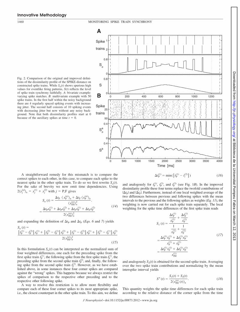
to correctly reflect long-term changes in spike train synchrony. However,as already noted in Kreuz et al. (2011), each individual instantaneousvalue in itself is less reliable since spuriously high values are obtainedduring slightly unreliable spiking events. This can be seen in the bivariateexample of Fig. 2A, where we use a frequency mismatch to construct twospike trains with gradually varying spike matches. In the first half thespikes in the second spike train exhibit increasing distances to thepreceding spikes of the first spike train, while in the second half theymove closer and closer to its following spikes. Thus we expect amonotonic increase of the instantaneous values followed by a monotonicdecrease. These two trends can indeed be recognized. However, they areinterrupted by short intervals of spurious high values.

The same kind of spurious high values can be seen in Fig. 2B forthe averaged bivariate variant So

a(t) in a multivariate example. Here inthe first half we generated four spiking events with increasing jitterwithin a noisy background, whereas the second half consists of evenlyspaced firing events with increasing precision, this time without anybackground noise. In both cases the spurious high values appear insmall intervals during which some of the spikes are still followingspikes while others are already preceding spikes. In these intervals thesmall differences between the spikes within the event are not takeninto account. Instead, because of the separation of preceding andfollowing spikes, the “wrong” spikes are compared to each other.Some of the differences among the preceding spikes as well as amongthe following spikes are very large, and this, according to Eq. 13,leads to the high instantaneous values.

0 1 2 3 4 5 6 7 8 9 10 11

A

1

2

Spike

trains

t(1)P

(t) t(1)F

(t)

t(2)P

(t) t(2)F

(t)

x(1)ISI

(t)

x(2)ISI

(t)

|∆ tP (t)| |∆ t

F (t)|t

<xPn(t)>

n<x

Fn(t)>

n

0 1 2 3 4 5 6 7 8 9 10 11

B

1

2

Spike

trains

Time [arbitrary unit]

t

t(1)P

(t) t(1)F

(t)

t(2)P

(t) t(2)F

(t)

x(1)P

(t)

x(2)P

(t)

x(1)F

(t)

x(2)F

(t)

|∆ tP(1) (t)|

|∆ tP(2) (t)|

|∆ tF(1) (t)|

|∆ tF(2) (t)|

Fig. 1. Illustration of the bivariate SPIKE-distance.A: local quantities in relation to time instant t neededto define the original dissimilarity profile (Eq. 13) ofthe SPIKE-distance. B: additional definitions used forthe improved dissimilarity profile (Eqs. 17 and 19)and its real-time variant (Eq. 21).

Innovative Methodology

1459MONITORING SPIKE TRAIN SYNCHRONY

J Neurophysiol • doi:10.1152/jn.00873.2012 • www.jn.org

at Biblioteca de la U

niversitat Pom

peu Fabra on M

arch 12, 2013http://jn.physiology.org/

Dow

nloaded from

A straightforward remedy for this mismatch is to compare thecorrect spikes to each other, in this case, to compare each spike to thenearest spike in the other spike train. To do so we first rewrite So(t).For the sake of brevity we now omit time dependencies. Using2�xj

�n��n � xj�1� � xj

�2� with j � P,F gives

So (t) ��tP � xF

(n)�n � �tF �xP(n)�n

�xISI(n)�n

2 .

��tPxF

(1) � �tPxF(2) � �tFxP

(1) � �tFxP(2)

2�xISI(n)�n

2

(14)

and expanding the definition of �tP and �tF (Eqs. 6 and 7) yields

So (t) �

�tP(1) � tP

(2)�xF(1) � �tP

(2) � tP(1)�xF

(2) � �tF(1) � tF

(2)�xP(1) � �tF

(2) � tF(1)�xP

(2)

2�xISI�n��n

2

(15)

In this formulation So(t) can be interpreted as the normalized sum offour weighted differences, one each for the preceding spike from thefirst spike train tP

(1), the following spike from the first spike train tF(1), the

preceding spike from the second spike train tP(2), and, finally, the follow-

ing spike from the second spike train tF(2). However, as we have estab-

lished above, in some instances these four corner spikes are comparedagainst the “wrong” spikes. This happens because we always restrict thespikes of comparison to the respective other preceding and to therespective other following spike.

A way to resolve this restriction is to allow more flexibility andcompare each of these four corner spikes to its most appropriate spike,i.e., the closest counterpart in the other spike train. To this aim, we define

�tP(1) � min

i(�tP

(1) � ti(2)�) (16)

and analogously for tF(1), tP

(2), and tF(2) (see Fig. 1B). In the improved

dissimilarity profile these four terms replace the twofold contributions of|�tP| and |�tF|. Furthermore, instead of one local weighted average of thetwo differences between previous and following spikes with the meanintervals to the previous and the following spikes as weights (Eq. 11), theweighting is now carried out for each spike train separately. The localweighting for the spike time differences of the first spike train reads

S1 (t) �

�tP(1)

xP(1) �

�tF(1)

xF(1)

1

xP(1) �

1

xF(1)

��tP

(1)xF(1) � �tF

(1)xP(1)

xF(1) � xP

(1)

��tP

(1)xF(1) � �tF

(1)xP(1)

xISI(1)

(17)

and analogously S2(t) is obtained for the second spike train. Averagingover the two spike train contributions and normalizing by the meaninterspike interval yields

S � (t) �S1(t) � S2(t)

2�xISI(n) (t)�n

. (18)

This quantity weights the spike time differences for each spike trainaccording to the relative distance of the corner spike from the time

0 200 400 600 800 1000 12000

0.8

0

0.8

2

1Spike

trains

S

So

A

0 500 1000 1500 2000 2500 3000 3500 40000

0.4

0

0.4

50

25Spike

trains

Sa

Soa

Time [ms]

B

Fig. 2. Comparison of the original and improved defini-tions of the dissimilarity profile of the SPIKE-distance onconstructed spike trains. While So(t) shows spurious highvalues for eventlike firing patterns, S(t) reflects the levelof spike train synchrony faithfully. A: bivariate example:varying spike matches. B: multivariate example with 50spike trains. In the first half within the noisy backgroundthere are 4 regularly spaced spiking events with increas-ing jitter. The second half consists of 10 spiking eventswith decreasing jitter but now without any noisy back-ground. Note that both dissimilarity profiles start at 0because of the auxiliary spikes at time t � 0.

Innovative Methodology

1460 MONITORING SPIKE TRAIN SYNCHRONY

J Neurophysiol • doi:10.1152/jn.00873.2012 • www.jn.org

at Biblioteca de la U

niversitat Pom

peu Fabra on M

arch 12, 2013http://jn.physiology.org/

Dow

nloaded from

instant under investigation. In this way, relative distances within eachspike train are taken care of, while relative distances between spiketrains are not. To get these ratios straight and to account for differ-ences in firing rate, in a last step the two contributions from the twospike trains are locally weighted by their instantaneous interspikeintervals. This leads to the improved definition of the dissimilarityprofile:

S (t) �S1 (t)xISI

�2�(t) � S2 (t)xISI�1�(t)

2�xISI(n) (t)�n

2 . (19)

For many time instants the closest spike to the preceding spike of onespike train is the preceding spike in the other spike train and the sameholds for the following spikes, so often the same spikes are stillcompared to each other. However, for the time instants that led to thespurious high values for So(t) now the two preceding and the twofollowing spikes are no longer compared to each other. Instead, if afollowing spike in one spike train is the closest spike to a precedingspike of the other spike train (or vice versa) these will now becompared to each other, which leads to lower instantaneous values inthe dissimilarity profile.

This modification resolves the problem of spurious high values and,as can be seen in Fig. 2, the desired dissimilarity profiles are obtained.In Fig. 2A the observed monotonic increase of the instantaneousvalues followed by a monotonic decrease mirrors exactly the actualchange in the match between the spike times of the two spike trains.For the multivariate example of Fig. 2B and the averaged bivariatevariant (calculated according to Eq. 2) we find in the first half highinstantaneous values that reflect the background noise. The presenceof four spiking events with increasing jitter within this noisy back-ground is indicated by less and less pronounced drops in the dissim-ilarity profile. In the second half, where there is no background noise,the evenly spaced firing events with increasing precision are correctlyreflected by a rather monotonic decrease of the instantaneous syn-chrony level that reaches 0 at the perfectly synchronous event at3,900 ms. Such perfect events for which the value 0 is obtained aremarked by vertical dashed lines in the dissimilarity profile.

The firing rate correction introduced between Eqs. 18 and 19 hasthe important and desirable consequence that the SPIKE-distancebetween Poisson spike trains increases with the difference in firingrate (results not shown).

Real-time SPIKE-distance. Here we introduce the real-time SPIKE-distance DSr

. This is a modification of the SPIKE-distance with thekey difference that the corresponding time profile Sr(t) can be calcu-lated online because it relies on past information only. From theperspective of an online measure, the information provided by thefollowing spikes, both their position and the length of the interspikeinterval, is not yet available. Like the regular (improved) SPIKE-distance DS, this causal variant is also based on local spike timedifferences, but now only two corner spikes are available and thespikes of comparison are restricted to past spikes, e.g., for thepreceding spike of the first spike train

�tP(1) � min

i(�tP

(1) � ti(2)�), ti � t (20)

Since there are no following spikes available, there is no localweighting, and since there is no interspike interval, the normalizationis achieved by dividing the average corner spike difference by twicethe average time interval to the preceding spikes (Eq. 9; see also Fig.1B). This yields a causal indicator of local spike train dissimilarity:

Sr (t) ��tP

(1) � �tP(2)

4�xP(n)�n

. (21)

In Fig. 3 we show the results of the real-time SPIKE-distance forthe two cases already used in Fig. 2. As can be seen for the exampleof two spike trains with gradually varying spike mismatches (Fig. 3A),any spike time difference is considered most relevant right at the later

of two spikes when Sr(t) goes back to a local maximum value. In thecase where the two preceding spikes are closest to each other, it goesback to its maximum value of 1. At these points the mean time intervalto the two preceding spikes is exactly half their difference. Anysuccessive period of common nonspiking leads to a decrease of theinstantaneous distance values. This is a desired property since com-mon nonspiking is as much a sign of synchrony as common spiking.The decrease is hyperbolic, and its slope depends on the precedingspike time difference.

In addition to the regular trace we also show here a moving averagethat, in line with the real-time calculation, is causal. While the regulardissimilarity profile exhibits certain fluctuations, this moving averageshows that the real-time SPIKE-distance in fact reflects the increasingspike shifts in the center of the interval and the better match of thespike times at the edges.

During irregular spiking in the multivariate example of Fig. 3B, thetime intervals to the preceding spikes in different spike trains are veryvariable, and this leads to large fluctuating values of Sr

a(t). Within thisirregularity, the perfect spiking event at 400 ms results in an abruptdrop to 0, which reflects the delta distribution of the time intervals tothe preceding spikes. The successively more jittered events that followare indicated by a very pronounced short-term increase, followed bya decrease. Here the distribution of time intervals to preceding spikesstarts to develop a peak at very small intervals and thus becomesbimodal, which causes the increase. Then, after spikes have appearedin quick succession in all spike trains, the distribution becomes verynarrow, which is reflected by the decrease. In the second half, whenthere is no background noise and the spiking events become less andless noisy, the succession of peaks denoting the events is becomingmore and more prominent, with increasing amplitude range butnarrower base. Just as in the bivariate case, the short timescalefluctuations in this multivariate example can be eliminated by anappropriate (causal) moving average. Here this moving average ex-hibits a gradual decrease, which reflects the consistent increase of thespike event reliability.

It is important to note that, in contrast to the noncausal SPIKE-distance (see Fig. 2), the observed peaks are not spurious. They occurat time instants when it is not yet known whether there will in fact bea reliable spiking event or not. This is illustrated in Fig. 4 with twospiking events that are identical (1 spike per spike train) except for theomitted second half of the second event. While for both events theinstantaneous values in the first part necessarily have to be identical(and very high since only some of the neurons have recently spiked),the differences in the second part become evident as more and moreinformation becomes available. For the first event, once all neuronshave fired, a rapid decrease of Sr

a(t) can be observed, while the lowerfiring reliability in the second event leads to a slow decrease.

Practical considerations. The improved dissimilarity profile S(t) ofthe SPIKE-distance is piecewise linear (with each linear intervalrunning from one spike of the pooled spike train to the next) ratherthan piecewise constant as is the case for the ISI-distance. Therefore,when the localized visualization is desired, a new value has to becalculated for each sampling point and not just once per each intervalin the pooled spike train. In cases where the distance value itself issufficient, the short computation time can be even further decreasedby representing each interval by the value of its center and weightingit by its length. Not only is this faster, but it actually gives the exactresult, whereas the time-resolved calculation is a very good approxi-mation only for sufficiently small sampling intervals dt (imagine theexample of a rectangular function: at some point any sampled repre-sentation has to cut the right angle). The dissimilarity profile Sr(t) ofthe real-time SPIKE-distance is hyperbolic and not linear, but herealso the exact result can be obtained by piecewise integration over allintervals of the pooled spike train.

The calculation of the SPIKE-distance consists of three steps: In aprecalculation step, for each spike the distance to the nearest spike inall the other spike trains is calculated. Successively, for each time

Innovative Methodology

1461MONITORING SPIKE TRAIN SYNCHRONY

J Neurophysiol • doi:10.1152/jn.00873.2012 • www.jn.org

at Biblioteca de la U

niversitat Pom

peu Fabra on M

arch 12, 2013http://jn.physiology.org/

Dow

nloaded from

instant and each pair of spike trains, the distances of the four cornerspikes are first locally weighted and then normalized. These lattersteps involve matrices of the order “number of time instants” �“number of spike train pairs,” which for very long data sets with manyspike trains can lead to memory problems. The solution to these

problems is to make the calculation sequential, i.e., to cut the record-ing interval into smaller segments and to perform the averaging overall pairs of spike trains for each segment separately (no additionalauxiliary spikes are needed except for very huge data sets, for whicheven the calculation of the first matrix is too memory demanding). Inthe end, the dissimilarity profiles for the different segments (alreadyaveraged over pairs of spike trains) are concatenated, and its temporalaverage yields the distance value for the whole recording interval.

The computational load scales with the number of spike trains N asN2. With MATLAB on a notebook with a 2.53 GHz Intel Core 2 Duoprocessor the calculation of most of the examples in this article tookjust a few seconds, while the slowest example (the single-unit record-ings analyzed in Fig. 9) took �5 min.

More information on the implementation as well as the MATLABsource code for calculating and visualizing both the ISI-distance andthe SPIKE-distance (including the real-time variant) can be found atwww.fi.isc.cnr.it/users/thomas.kreuz/sourcecode.html.

RESULTS

Application to artificially generated data: instantaneousclustering. By eliminating the spurious high values in So

a(t), wehave gained reliability of Sa(t) for each time instant. Thisallows us to use the instantaneous matrices of pairwise spiketrain dissimilarities to divide the spike trains into clusters, i.e.,groups of spike trains with low intragroup and high intergroupdissimilarity. There are no limits to the temporal resolution;such a clustering can, in principle, be obtained for each timeinstant.

0 200 400 600 800 1000 12000

1

2

1Spike

trains

Sr

Sr

A

0 500 1000 1500 2000 2500 3000 3500 40000

0.5

50

25

Spike

trains

SraSra

Time [ms]

B

Fig. 3. Time profile of the real-time SPIKE-distance forthe two examples used in Fig. 2. In both subplots regulartraces are depicted by thin lines, while the causal movingaverages are shown by thick lines. A: bivariate example.While the regular dissimilarity profile Sr(t) attains a localmaximum for each spike, its subsequent decay still cap-tures the relative spiking behavior. This can be seen bestwith the moving average, which reflects the correct long-term trends. B: multivariate example. The averaged bi-variate dissimilarity profile Sr

a(t) exhibits periods of highvalues in certain intervals, but in contrast to the originalnoncausal case So

a(t), these are not spurious (see Fig. 4).

0 50 100 150 0 50 100 1500

0.5

50

25

Spike

trains

Sra

Time [ms]

Fig. 4. Real-time SPIKE-distance: peaks during reliable spiking events are notspurious: multivariate example with 2 spiking events that have identical first halvesbut different continuations. After 100 ms some of the neurons have just spikedwhile others have been silent for some time, and for both events this largevariability is correctly reflected by high values of the averaged bivariate dissimi-larity profile Sr

a(t). At these points begin the shaded areas that mark the spikeinformation that is not yet available. Here for the first event the initial spiking insome of the spike trains turns into a reliable spiking event (1 spike for each spiketrain), which is reflected by a rapid decrease to very low values. For the secondevent this does not happen, and accordingly the decrease is less pronounced.

Innovative Methodology

1462 MONITORING SPIKE TRAIN SYNCHRONY

J Neurophysiol • doi:10.1152/jn.00873.2012 • www.jn.org

at Biblioteca de la U

niversitat Pom

peu Fabra on M

arch 12, 2013http://jn.physiology.org/

Dow

nloaded from

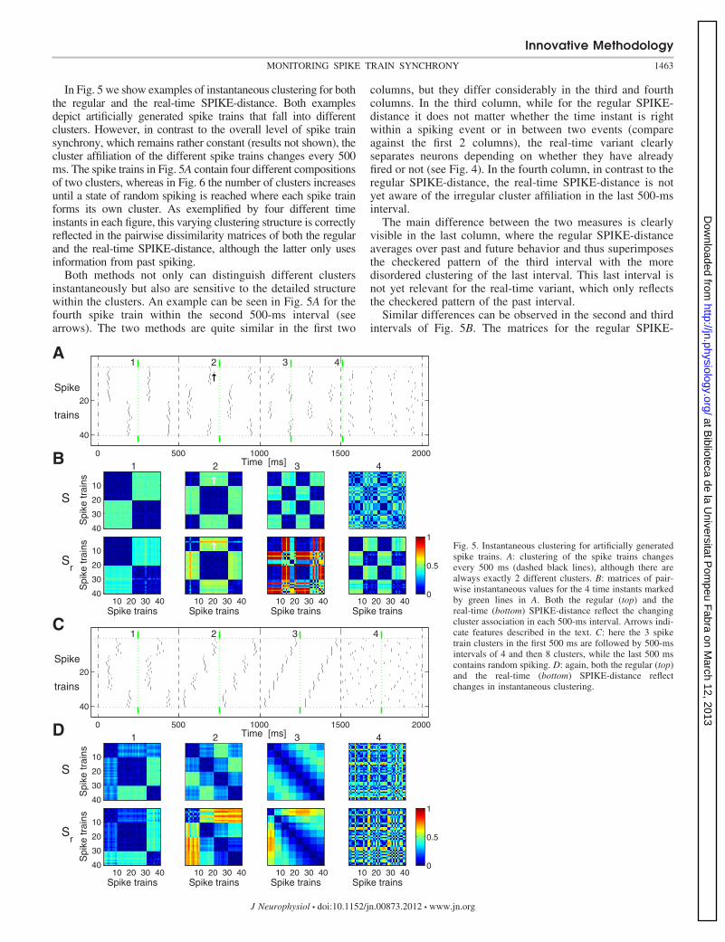
In Fig. 5 we show examples of instantaneous clustering for boththe regular and the real-time SPIKE-distance. Both examplesdepict artificially generated spike trains that fall into differentclusters. However, in contrast to the overall level of spike trainsynchrony, which remains rather constant (results not shown), thecluster affiliation of the different spike trains changes every 500ms. The spike trains in Fig. 5A contain four different compositionsof two clusters, whereas in Fig. 6 the number of clusters increasesuntil a state of random spiking is reached where each spike trainforms its own cluster. As exemplified by four different timeinstants in each figure, this varying clustering structure is correctlyreflected in the pairwise dissimilarity matrices of both the regularand the real-time SPIKE-distance, although the latter only usesinformation from past spiking.

Both methods not only can distinguish different clustersinstantaneously but also are sensitive to the detailed structurewithin the clusters. An example can be seen in Fig. 5A for thefourth spike train within the second 500-ms interval (seearrows). The two methods are quite similar in the first two

columns, but they differ considerably in the third and fourthcolumns. In the third column, while for the regular SPIKE-distance it does not matter whether the time instant is rightwithin a spiking event or in between two events (compareagainst the first 2 columns), the real-time variant clearlyseparates neurons depending on whether they have alreadyfired or not (see Fig. 4). In the fourth column, in contrast to theregular SPIKE-distance, the real-time SPIKE-distance is notyet aware of the irregular cluster affiliation in the last 500-msinterval.

The main difference between the two measures is clearlyvisible in the last column, where the regular SPIKE-distanceaverages over past and future behavior and thus superimposesthe checkered pattern of the third interval with the moredisordered clustering of the last interval. This last interval isnot yet relevant for the real-time variant, which only reflectsthe checkered pattern of the past interval.

Similar differences can be observed in the second and thirdintervals of Fig. 5B. The matrices for the regular SPIKE-

0 500 1000 1500 2000

40

20

Spike

trains

Time [ms]

A1 2 3 4

S

Spi

ke tr

ains

B 1

10

20

30

40

2 3 4

Spike trains

Sr

Spi

ke tr

ains

10 20 30 40

10

20

30

40

Spike trains10 20 30 40

Spike trains10 20 30 40

Spike trains10 20 30 40

0

0.5

1

0 500 1000 1500 2000

40

20

Spike

trains

Time [ms]

C1 2 3 4

S

Spi

ke tr

ains

D 1

10

20

30

40

2 3 4

Spike trains

Sr

Spi

ke tr

ains

10 20 30 40

10

20

30

40

Spike trains10 20 30 40

Spike trains10 20 30 40

Spike trains10 20 30 40

0

0.5

1

Fig. 5. Instantaneous clustering for artificially generatedspike trains. A: clustering of the spike trains changesevery 500 ms (dashed black lines), although there arealways exactly 2 different clusters. B: matrices of pair-wise instantaneous values for the 4 time instants markedby green lines in A. Both the regular (top) and thereal-time (bottom) SPIKE-distance reflect the changingcluster association in each 500-ms interval. Arrows indi-cate features described in the text. C: here the 3 spiketrain clusters in the first 500 ms are followed by 500-msintervals of 4 and then 8 clusters, while the last 500 mscontains random spiking. D: again, both the regular (top)and the real-time (bottom) SPIKE-distance reflectchanges in instantaneous clustering.

Innovative Methodology

1463MONITORING SPIKE TRAIN SYNCHRONY

J Neurophysiol • doi:10.1152/jn.00873.2012 • www.jn.org

at Biblioteca de la U

niversitat Pom

peu Fabra on M

arch 12, 2013http://jn.physiology.org/

Dow

nloaded from

distance are quite symmetrical with respect to the dissimilari-ties to the different clusters since the increasing distancesbetween the preceding spikes are balanced by the decreasingdistances to the following spikes. In contrast, the real-timeSPIKE-distance reflects the increasing distance between thepreceding spikes only. Thus, although the spike time differ-ences between adjacent groups are similar, because of thenormalization lower dissimilarities are obtained for groups ofspike trains whose spikes are further in the past.

So far we have shown clustering matrices obtained at certaintime instants. Since such a matrix exists for each and every timeinstant t, it is possible to selectively average over certain timeintervals. These intervals do not have to be continuous; selectiveaveraging over separated intervals is possible as well. Four ex-amples are shown in Fig. 6, an average over one individual500-ms interval, averages over two consecutive as well as twoseparated 500-ms intervals, and finally the average over thewhole time interval. In each case a linear superposition of theindividual matrices can be observed. For the whole interval(Fig. 6B, 4th column) this means that the four groups of 10spike trains that frequently belonged to the same cluster canstill be identified (see arrow). Because there were two 500-msintervals (the 2nd and the 5th) where the second and the thirdspike train group formed one big cluster, these two groups aremore closely related than the other groups, which is correctlyreflected by the lower values of dissimilarity.

Another option is triggered temporal averaging. Here thematrices are averaged over certain trigger time instants only.The idea is to check whether this triggered temporal average is

significantly different from the global average, since this wouldindicate that something peculiar is happening at these triggerinstants.

The trigger times can be obtained either from internalconditions (such as the spike times of a certain spike train) orfrom external influences (such as the occurrence of certainfeatures in a stimulus).

An example of internal triggering can be seen in Fig. 7, A–C.In this artificially generated setup there are 20 simultaneouslyrecorded neurons and almost all of them fire independentlyfrom each other, following a Poisson statistic (Fig. 7A). Theexception is the first neuron, which fires at a lower rate and isassumed to have a strong excitatory synaptic coupling to five ofthe other neurons (4, 8, 11, 16, and 19). Correspondingly, thespike trains of these neurons were modified such that theycontained slightly lagged and jittered copies of the spikes of thefirst spike train in addition to spikes generated independently.This represents a situation in which each spike in the first spiketrain causes (triggers) a spike in these spike trains, but there arealso other spikes (which might have been caused by differentneurons that were not recorded).

The task is to identify these five neurons. This is verydifficult via visual inspection, and also the overall temporalaverage is unable to do so (Fig. 7B, left). However, theseneurons can be identified by averaging over the pairwiseinstantaneous values obtained for the spike times of the firstspike train (the internal trigger instants) only. The resultingdissimilarity matrix shown in Fig. 7B, right, includes anirregular grid of very small distance values.

0 500 1000 1500 2000 2500 3000 3500 4000

40

30

20

10

A

Time [ms]

Spike

trains

12

334

Spi

ke tr

ains

S

B 1

10

20

30

40

2 3 4

Spike trains

Spi

ke tr

ains

Sr

10 20 30 40

10

20

30

40

Spike trains10 20 30 40

Spike trains10 20 30 40

Spike trains10 20 30 40

0

0.5

1

Fig. 6. Selective temporal averaging. A: the spiketrains are concatenated from the 2 examples in Fig. 5.B: each column (from left to right) depicts the selec-tive temporal average over the intervals marked by thehorizontal lines in A (from top to bottom). Arrowsindicate features described in the text.

Innovative Methodology

1464 MONITORING SPIKE TRAIN SYNCHRONY

J Neurophysiol • doi:10.1152/jn.00873.2012 • www.jn.org

at Biblioteca de la U

niversitat Pom

peu Fabra on M

arch 12, 2013http://jn.physiology.org/

Dow

nloaded from

Another representation of dissimilarity matrices is hierarchi-cal cluster trees also known as dendrograms (Fig. 7C). Theyare constructed as follows: First, the closest pair of spike trainsis identified and thereby linked by a �-shaped line, where theheight of the connection measures the mutual distance. Thesetwo time series are merged into a single element, and the nextclosest pair of elements is then identified and connected. Theprocedure is repeated iteratively until a single cluster remains.The implementation of this method requires introducing thedistance between a pair of clusters. In the single linkagealgorithm used here, this distance is defined as the minimumover all the distances between pairs of spike trains in the twoclusters. In Fig. 7C, the dendrogram obtained from the averagedissimilarity matrix (Fig. 7C, left) does not fall into separateclusters, whereas in the dendrogram of the triggered average

(Fig. 7C, right) the five modified spike trains form one distinctcluster with the first spike train and can thus easily beidentified.

In contrast to internal triggering, externally triggered aver-aging allows certain (external) stimulus features to be relatedwith spike train synchrony and might thus be a promising toolfor the investigation of neuronal coding. While the example forinternal triggering assumes a simultaneously recorded popula-tion of neurons, in the setup of the external triggering example(Fig. 7, D–F) just one neuron is recorded for repeated stimu-lation with the same stimulus. This stimulus is a chirp function,representative of a nonperiodic time-varying stimulus. It isassumed that the neuron is sensitive to negative amplitudes andaccordingly it exhibits higher (lower) reliability for local min-ima (maxima) of the chirp function (Fig. 7D). However, to

0 10 20 30 40 50 60 70 80 90 100

20

10

Spi

ke tr

ains

A

Time [ms]

12

10 2020

10

Spike trains

Spi

ke tr

ains

S

1B

8 1116 2 4 18201519 9 101214 7 17 3 13 5 6 1Spike trains

C10 20

20

10

Spike trains

Spi

ke tr

ains

2

0

0.5

1

1 161119 8 4 12 9 20 6 5 1814 2 101517 3 13 7Spike trains

0 500 1000 1500 2000 2500 3000 3500 4000 4500 500040

20

D

Spi

ke tr

ains

Stim

ulus

Time [ms]

1234

20 40

10

20

30

40

Spike trains

Spi

ke tr

ains

S

E 1

Spike trains

F20 40

Spike trains

2

Spike trains

20 40Spike trains

3

Spike trains

20 40Spike trains

4

0

0.5

1

Spike trains

Fig. 7. Triggered temporal averaging. A–C:internal triggering. A: Poisson spike trainswith superimposed firing patterns: 5 spiketrains (4, 8, 11, 16, and 19, marked by hori-zontal red lines) follow the spiking of the firstspike train (with small amounts of jitter).Below the horizontal line denoting the overallaverage, triangles mark the spike times of thefirst spike train, which are used as triggerinstants. B: dissimilarity matrices (for the reg-ular SPIKE-distance): averaging over thewhole interval (left) and averaging over theinstantaneous matrices at all trigger instantsonly (right). C: hierarchical cluster trees (den-drograms) obtained from the dissimilarity ma-trices in B. D–F: external triggering. D: arti-ficially generated spike trains. While one halfof the neurons are noisy, the synchrony of theother half is modulated via a chirplike externalstimulus (shown at top). These nonperiodi-cally varying levels of synchrony can betraced by triggering on time instants withcommon stimulus amplitude (marked by hor-izontal green lines and green triangles). E: dis-similarity matrices. Each column (from left toright) depicts the externally triggered tempo-ral average for decreasing amplitudes of thechirp function (from top to bottom in A, top).F: corresponding dendrograms. As the emergingspike train cluster shows, lower stimulus ampli-tudes lead to increased levels of synchrony.

Innovative Methodology

1465MONITORING SPIKE TRAIN SYNCHRONY

J Neurophysiol • doi:10.1152/jn.00873.2012 • www.jn.org

at Biblioteca de la U

niversitat Pom

peu Fabra on M

arch 12, 2013http://jn.physiology.org/

Dow

nloaded from

better illustrate the gradual increase in clustering, half the trialswere left unaffected from the stimulus.

As the amplitude of the chirp function varies, so does thespike train synchrony of half of the trials. Because of thenonperiodicity of the stimulus this is quite difficult to detect.Detection is facilitated by externally triggered averaging wherethe triggering is performed on common stimulus features (inthis example the amplitude of the chirp function). As can beseen in the dissimilarity matrices (Fig. 7E) and even better inthe dendrogram (Fig. 7F), a decrease of this stimulus amplitudeleads to the emergence of a spike train cluster consisting of themodulated spike trains, which indicates their increase inreliability.

In the Supplemental Material we present SupplementalMovie S1, which uses the artificially generated spike trainsfrom Figs. 5 and 6 and includes instantaneous clustering,selective temporal averaging of individual or combined inter-vals, several examples of triggered averaging, as well as thecorresponding dendrograms.1 As can be seen in the screenshotof the movie shown in Fig. 8, we added one more feature, thecomparison of spike train groups, where the spike trains are manuallyassigned to subgroups and a block matrix (and the correspondingdendrogram) is obtained by averaging over the respective subma-trices of the original dissimilarity matrix. For both distances

these spatial averages over groups of spike train pairs aredenoted by �•�G.

Application to single-unit recordings from epilepsy patients.In all previous examples we have used artificially generatedspike trains for which the relative levels of spike train syn-chrony were known and could serve as validation for the spiketrain distances. Here we present an exemplary application ofboth the SPIKE-distance and its real-time variant to field datafor which no a priori knowledge is available. As field data wechose recordings of neuronal spiking from the human medialtemporal lobe. These recordings were performed at the Uni-versity of Bonn in epilepsy patients undergoing seizure mon-itoring prior to epilepsy surgery. For a description of the datarefer to APPENDIX B.

In Fig. 9A we show the spike trains recorded from 42 singleunits and multiunits of an epilepsy patient during an epoch thatcontained an epileptic seizure. For this particular patient theepileptic focus was later confirmed to lie in the hippocampalformation of the left brain hemisphere. In this example theSPIKE-distance and its real-time variant exhibit a rather lim-ited amount of variability before and after the epileptic seizure,while during the seizure both distances exhibit strong fluctua-tions, particularly during the second part of the seizure whenthe local field potentials exhibit high-amplitude rhythmic ac-tivity (data not shown). Remarkably, both distances show apronounced drop at the beginning of the seizure, at a time whenonly subtle changes are discernible in the continuous local field

1 Supplemental Material for this article is available online at the Journalwebsite.

0 500 1000 1500 2000 2500 3000 3500 4000

40

30

20

10

A

G1

G2

G3

G4

Time [ms]

10 20 30 4040

30

20

10

Spike trains

Spi

ke tr

ains

SB

Spike trains

C10 20 30 40Spike trains

Sr

Spike trains

G1 G2 G3 G4

G4

G3

G2

G1

Spike train groups

Spi

ke tr

ain

grou

ps

< S >G

1 4 2 3Spike train groups

G1 G2 G3 G4Spike train groups

< Sr>

G

0

0.2

0.4

0.6

0.8

1

2 3 1 4Spike train groups

Fig. 8. Screenshot from Supplemental MovieS1. A: artificially generated spike trains.B: dissimilarity matrices obtained by averag-ing over 2 separate time intervals for both theregular and the real-time SPIKE-distance aswell as their averages over subgroups ofspike trains (denoted by �•�G). C: corre-sponding dendrograms.

Innovative Methodology

1466 MONITORING SPIKE TRAIN SYNCHRONY

J Neurophysiol • doi:10.1152/jn.00873.2012 • www.jn.org

at Biblioteca de la U

niversitat Pom

peu Fabra on M

arch 12, 2013http://jn.physiology.org/

Dow

nloaded from

0 1 2 3 4 5

0

0.6

0

0.6

42

3432

25

1712

6

Time [min]

LALAHLECLPHCRARAHREC

Sa

Sra

A1 2 3

Spi

ke tr

ains

S

B 1

10

20

30

40

2 3

Spike trains

Spi

ke tr

ains

Sr

10 20 30 40

10

20

30

40

Spike trains10 20 30 40

Spike trains10 20 30 40

0

0.2

0.4

0.6

0.8

1

Fig. 9. Exemplary application of the SPIKE-distance and its real-time variant to single-unit and multiunit recordings from an epilepsy patient (whose epilepticfocus was in the left hippocampal formation) before, during, and after an epileptic seizure. A: recorded spike trains and the 2 dissimilarity profiles (which startat 0 because of the auxiliary spikes at time t � 0) as well as their average values for the periods before, during, and after the epileptic seizure. Seizure onsetand offset are marked by vertical lines. Different brain regions (hemispheres) are separated by (thick) horizontal lines. LA, RA, left and right amygdala; LAH,RAH, left and right anterior hippocampus; LEC, REC, left and right entorhinal cortex; LPHC, left parahippocampal cortex. No units were recorded from rightparahippocampal cortex. B: selective temporal averaging. Each column (from left to right) depicts the selective average over the time interval marked by ahorizontal line (from top to bottom) in A (before, during, and after the epileptic seizure). The dashed (solid) lines separate values obtained for different brainregions (hemispheres).

Innovative Methodology

1467MONITORING SPIKE TRAIN SYNCHRONY

J Neurophysiol • doi:10.1152/jn.00873.2012 • www.jn.org

at Biblioteca de la U

niversitat Pom

peu Fabra on M

arch 12, 2013http://jn.physiology.org/

Dow

nloaded from

potential (data not shown). This could be an indication that anincreased level of synchrony among a population of neuronsplays an important role in the generation of seizure activity.

Figure 9B shows the dissimilarity matrices for both spiketrain distances averaged over the periods before, during, andafter the seizure. These matrices reflect the relationships be-tween all the neurons recorded from different regions of bothtemporal lobes. In the nonfocal hemisphere, i.e., the side of thebrain that does not contain the epileptic focus, neurons 26–42exhibit a constant pattern of synchrony before, during, andafter the seizure. In the focal hemisphere the general level ofspike distance is lower during the seizure than before orafterwards, indicating an elevated level of neuronal synchronyduring the seizure. The spike train distances between the twobrain hemispheres (Fig. 9B, top right and bottom left quad-rants) show a relatively high level of synchrony for the sparselyfiring neurons (26, 27, 28, 33, 34, and 37) that is substantiallydiminished during the seizure.

These findings are in line with standard theories on seizuredynamics (Engel and Pedley 2008). The spike train distancesthus appear to be suitable measures to describe the mechanismsof seizure generation, propagation, and termination at theneuronal level. Specifically, they provide an opportunity toextend our mechanistic understanding of spatiotemporal sei-zure dynamics by elucidating the functional role of synchro-nization and desynchronization processes. A separate analysisof spike train synchrony for different regions of the focal andnonfocal medial temporal lobe may provide additional insightsabout the evolution of a seizure (see Schevon et al. 2012).

The real-time variant could furthermore be integrated intoprospective algorithms aimed, e.g., at an early online detectionof seizure occurrence (Jouny et al. 2011).

Application to continuous data. To our knowledge, there areno time series analysis methods that allow reliable tracking ofinstantaneous synchrony in continuous data, i.e., to map theirlocal dissimilarity to one value for each time instant, eitheronce the complete segment is available for analysis or online inreal time. Now that we have provided such a method fordiscrete data, the question arises as to whether it is possible toextend their applicability to continuous data. Thus in the thirdapplication we use the SPIKE-distance and its real-time variantto measure time-resolved dissimilarity in continuous signals.For this purpose, a high temporal resolution is once againbeneficial since changes in synchronization can occur on verysmall timescales. Examples include the transition to seizureobservable in the EEG of epilepsy patients (Lopes da Silva etal. 2003).

The principal idea is to first transform the continuous timeseries into one or more sequences of discrete events that arechosen to capture the most relevant characteristics of the data.In the case of neuronal membrane potentials, these are thespikes. Under the assumption that both the shape of the spikeand the background activity carry minimal information, neu-ronal responses are reduced to a spike train in which the onlyinformation maintained is the timing of the individual spikes.For the rather oscillatory EEG data that we analyze here, eachcontinuous time series is transformed into two separate se-quences of local maxima and local minima; similar choiceswere made, for example, by Quian Quiroga et al. (2002) andKugiumtzis et al. (2004). The SPIKE-distance is applied toboth kinds of sequences, and the two resulting dissimilarity

profiles are averaged. As before, the temporal average of thiscombined profile yields the SPIKE-distance. For this type ofdata a causal calculation is also possible; the procedure is thesame as used above for the regular SPIKE-distance.

To validate the instantaneous measures of synchronizationon controlled continuous data, we used data freely available onthe internet via the EEG time series download page (www.meb.uni-bonn.de/epileptologie/science/physik/eegdata.html)of the Department of Epileptology at the University of Bonn(Andrzejak et al. 2001). We randomly selected N � 10 indepen-dent channels (sampling rate 173.16 Hz) and then introduced atime-dependent mixing parameter m. For m � 0 the originalindependent channels are maintained, whereas for m � 1/N allchannels are exactly identical. Intermediate values of m interpo-late linearly between these two extremes. Although not relevantfor the event detection, the variance, which is decreased for mixedsignals, is adjusted to maintain the appearance of a regular EEGsignal.

In Fig. 10A we show an illustration of the application of theaveraged bivariate SPIKE-distance and its real-time variant tocontinuous EEG data using just three channels over a shortinterval of time that includes a transition from independentchannels to perfectly synchronous channels. This transition istraced by both measures. Figure 10B depicts the dissimilarityprofiles of the two SPIKE-distances for alternating piecewiseconstant variations of the mixing parameter, which convergesstepwise toward an intermediate level. Both measures arecapable of monitoring these transitions in the level of synchro-nization. Starting from zero values for identical synchroniza-tion and high values for independent channels, two gradualtransitions can be observed. However, as the different gradientsshow, it is easier to trace deviations from identical signals thandeviations from independent signals.

DISCUSSION

There are three different contributions of this study. Wehave improved the dissimilarity profile of the SPIKE-distance(Kreuz et al. 2011) by eliminating the spurious high values thatwere previously obtained for eventlike firing patterns, we haveadded a variant of the SPIKE-distance that is causal and allowsreal-time calculation, and, finally, we have extended the appli-cability of both of these variants to continuous data (such asEEG).

The instantaneous reliability obtained by the elimination ofthe spurious high values has very important consequences. Inaddition to the improved capability to track the overall level ofsynchronization within a group of two or more spike trains (seeFigs. 2 and 3), it is now possible to visualize instantaneousclustering (Fig. 5 and Supplemental Movie S1), i.e., to repre-sent evolving patterns of (dis)similarity in multiple spike trainseither as instantaneous matrices of pairwise spike train dissim-ilarities or as hierarchical cluster trees (dendrograms). Sincesuch matrices and dendrograms exist for each and every timeinstant t, it is possible to selectively average over certain(continuous or noncontinuous) time intervals (Fig. 6), which donot have to have the same length (see also Fig. 9). In real datathese intervals could be chosen to correspond to differentexternal conditions such as normal versus pathological, asleepversus awake, target versus nontarget stimulus, or presence/absence of a certain channel blocker. The fact that there are no

Innovative Methodology

1468 MONITORING SPIKE TRAIN SYNCHRONY

J Neurophysiol • doi:10.1152/jn.00873.2012 • www.jn.org

at Biblioteca de la U

niversitat Pom

peu Fabra on M

arch 12, 2013http://jn.physiology.org/

Dow

nloaded from

limits to the temporal resolution allows further analyses such asinternally or externally triggered temporal averaging (see Fig.7). In real multineuron data, internal triggering might help touncover certain structures and patterns in neural networks or todetect converging or diverging patterns of firing propagation.External triggering might be used to address questions ofneuronal coding, e.g., it could be used to evaluate the influenceof localized stimulus features on the reliability of real neuronsunder repeated stimulation. Finally, another possibility is spa-tial averaging over spike train groups (see Fig. 8). In applica-tions to real data, these groups could be different neuronalpopulations or responses to different stimuli, depending onwhether the spike trains were recorded simultaneously orsuccessively.

The SPIKE-distance appears to provide a reliable time-resolved measure of spike train similarity without the need tooptimize a timescale parameter. This extends the range ofpossible neurophysiological applications of spike train similar-ity measures. In the past, methods aimed at measuring spiketrain similarity have been applied in very controlled situations,

typically protocols in which the animal is anesthetized and thesame stimulus is repeated over multiple trials. With the SPIKE-distance, it is envisaged that similarity-based approaches couldbe extended to experiments with awake, behaving animals: theidentical trials typically required to select an appropriate time-scale parameter are not required for the SPIKE-distance, andthe time resolution allows the similarity to be monitored duringbehavior or in response to complex evolving stimuli; forexample, the extent to which neurons in a population synchro-nize in response to stimuli could be analyzed.

In cases where the complete spike trains are known, theregular SPIKE-distance compares favorably against the real-time SPIKE-distance. It is locally more reliable because it hasinformation about both the past and the future at its disposal.For the real-time SPIKE-distance the lack of information aboutspikes that occur in the future leads to high values duringreliable spiking events. While these values are not spurious(see Fig. 4), they are not really informative since they reflectlocal uncertainty that can easily be resolved by incorporatingall the information available. However, in situations that de-

0 0.1 0.2 0.3 0.40

0.8

0

0.4

3

2

1

EEG

SaSa

SraSra

Time [s]

Time [s]

A

0 20 40 60 800

0.4

0

0.2

10

8

6

4

2

EEG

SaSa

SraSra

B

Fig. 10. Exemplary application of the aver-aged bivariate SPIKE-distance and its real-time variant to continuous data. A, top: 3continuous EEG signals of 0.5-s duration thatexhibit a transition from being independent tobeing perfectly synchronous after �0.5 s (themixing parameter is superimposed in green).The maxima and minima of the EEG signalsare marked in red and blue, respectively, andthe same colors are used for the dissimilarityprofiles obtained from applying the 2 SPIKE-distances to the respective event time seriesonly (bottom). For each SPIKE-distance theblack trace depicts the average over these 2profiles and the green trace its moving aver-ages. B, top: 10 mixed signals generated from10 different EEG channels by means of anoscillating mixing parameter. For maximummixing we obtain identical signals, while with-out mixing the original EEG channels arepreserved. Bottom: dissimilarity profiles of theaveraged bivariate SPIKE-distance and itsreal-time variant, respectively (black), as wellas their moving averages (green). The excerptused in A is marked by a small black box (seearrow).

Innovative Methodology

1469MONITORING SPIKE TRAIN SYNCHRONY

J Neurophysiol • doi:10.1152/jn.00873.2012 • www.jn.org

at Biblioteca de la U

niversitat Pom

peu Fabra on M

arch 12, 2013http://jn.physiology.org/

Dow

nloaded from

mand online monitoring, the real-time SPIKE-distance can berelied upon, as we could show both for simulated and fielddata. A good example for the latter is Fig. 9B, in which evenwith only half the information available the results achievedwere very similar to those for the regular SPIKE-distance(compare Fig. 9B, top and bottom).

The capability to monitor the synchrony between two ormore spike trains (or continuous recordings) in real time opensup new possibilities for several important applications. Syn-chronization has been hypothesized to play a pivotal role inneuronal coding (Miller and Wilson 2008), and thus a real-timetracker of spike train synchrony could be an essential tool forrapid online decoding with brain-machine interfaces in order tocontrol prosthetic devices (Hochberg et al. 2006; Mulliken etal. 2008; Sanchez et al. 2008). In epilepsy patients, monitoringthe spiking activity of large ensembles of single neurons couldlead to a better understanding of the mechanisms of seizuregeneration. Furthermore, if neuronal spiking patterns turn outto be specific predictors of seizure occurrence as reported by arecent study (Truccolo et al. 2011), the real-time SPIKE-distance could be a viable tool for the implementation of aprospective seizure prediction algorithm (Mormann et al.2007).

In a similar manner, the SPIKE-distance and its real-timevariant can be applied to monitor synchrony in continuous data(which are first transformed into discrete data, see Fig. 10).Even the analysis of mixed continuous-discrete signals ispossible (see also Andrzejak and Kreuz 2011). A potentialapplication could be the combined analysis of discrete spiketrains and continuous neuronal oscillations. In particular, itwould be interesting to investigate neuronal synchronizationpatterns in dependence of the phase of the local field potential,a scenario reminiscent of the “neuronal communication throughneuronal coherence” scenario (Fries 2005).

Note that there is a conceptual analogy between the im-proved definition of the SPIKE-distance and the similaritymeasure proposed by Hunter and Milton (2003), which basi-cally sums the exponentially weighted distances from eachspike to its nearest spike in the other spike train. However, themain difference, apart from the additional exponential weight-ing and the parameter (the decay constant of the exponential),is that the calculation is not done in a time-resolved manner bymeans of a local weighting of the terms of the four cornerspikes. Instead, the term for each spike is considered just once.The SPIKE-distance is a rather elementary measure that can beregarded as complementary to cross correlation. Both measuresrely on differences in spike timing. However, while the latterestimates spike synchrony in dependence on a time lag but isnot sensitive to instantaneous synchrony, the SPIKE-distanceestimates instantaneous synchrony but is not sensitive to timelags (these should be eliminated beforehand).

Below we provide an overview of the main properties ofboth the SPIKE-distance and its real-time variant.

Straightforward extension to multiple spike trains andnormalization. The SPIKE-distance directly addresses the lackof approaches to analyze multiple spike train data (Brown et al.2004). It can readily be applied to very large data sets (some ofthe data sets analyzed contained �100 spike trains with a totalof almost 250,000 spikes). Both the bivariate and averagedbivariate distance are normalized between 0 and 1, where 0 is

obtained for identical spike trains only. The same limits holdfor the underlying dissimilarity profiles.

Different levels of information reduction. For the SPIKE-distance there are three different levels of information reduc-tion. The starting point is the most detailed representation inwhich one instantaneous value is obtained for each pair ofspike trains. The resulting matrix of size “number of sampledtime instants” � “squared number of spike trains” [i.e.,#(tn)N2] can be appreciated best in a movie; an example can befound in the Supplemental Material. For the first step ofinformation reduction there are two possible averages: theaverage over spike train pairs and the temporal average. Thesecommute; either can be performed first. By averaging instan-taneously over all pairs of spike trains a dissimilarity profile forthe whole population (e.g., Fig. 2) is obtained, whereas thetemporal averaging leads to a bivariate distance matrix (e.g.,Fig. 5). Finally, in both cases the second average leads to onedistance value that describes the overall level of synchrony fora group of spike trains over a given time interval. Note thathere we restricted the analysis to average values, but theapplication of higher-order statistics (such as the variance) isalso conceivable. Depending on the application in mind, theappropriate representation can be chosen. Mapping the simi-larity of a whole population onto one single value might allowfor an easier comparison, but one might lose too much infor-mation since high and low spike time differences at differenttime instants or for different pairs of spike trains might canceleach other out, leading to a value that could also be obtainedfor a constant intermediate level of similarity. This is oneexample where a higher-order statistic such as the variancecould be useful.

High temporal resolution: reliance on local information,then global averaging. The SPIKE-distance relies on instanta-neous values that only take into account local information frompreceding and—with the exception of the real-time SPIKE-distance—following spikes. Temporal averaging (Eq. 1) thenyields a more global picture by means of a single-valuedistance. The fact that the averaging window can be chosenarbitrarily allows for easy comparisons between the levels ofspike train synchrony in different time intervals without theneed for recalculations. The high temporal resolution thatrenders a sliding-window analysis obsolete compares themfavorably to other widespread measures of spike train variabil-ity such as the Fano factor.

Dependence on spike train of origin. The SPIKE-distancetakes into account the spike train of origin for each individualspike, and it is not invariant to shuffling spikes among the spiketrains. This is in contrast to measures that act on the pooledspike train, such as all measures based on the peristimulus timehistogram (PSTH), which yield the same value regardless ofhow spikes are distributed among the different spike trains andcould possibly fail to distinguish between qualitatively differ-ent behaviors such as high-reliability spiking and chain-firebursting (see Kreuz et al. 2011).

Computational efficiency. The SPIKE-distance is based onsimple differences and ratios that furthermore can easily beparallelized. For a large set of very long spike trains for whichcomputer memory might be a concern, the dissimilarity profilefor successive intervals can be calculated sequentially.

Timescale independence and absence of parameters. TheSPIKE-distance is invariant to stretching and compressing of

Innovative Methodology

1470 MONITORING SPIKE TRAIN SYNCHRONY

J Neurophysiol • doi:10.1152/jn.00873.2012 • www.jn.org

at Biblioteca de la U

niversitat Pom

peu Fabra on M

arch 12, 2013http://jn.physiology.org/

Dow

nloaded from

the spike trains. It is also timescale adaptive since the infor-mation used at each time instant is not contained within awindow of fixed size but within a time interval whose sizedepends on the local rates of the spike trains. In contrast totimescale-dependent measures such as the Victor-Purpura dis-tance (Victor and Purpura 1996) or the van Rossum distance(van Rossum 2001), parameter-free single-valued methodsgive a more objective and comparable estimate of neuronalvariability. Other drawbacks of timescale-dependent measuresare the computational cost and the time and effort that areneeded to find the right parameter. Moreover, it is not at allguaranteed that a right parameter exists.

One of the main arguments for the use of timescale-depen-dent measures of spike train (dis)similarity is their potentialinsight into the precision of the neuronal code (Victor andPurpura 1996). This argument has recently been reevaluated byChicharro et al. (2011). According to this study the optimaltimescale obtained from a spike train discrimination analysis isfar from being conclusive. Rather, it results in a nontrivial wayfrom the interplay of many different factors such as thedistribution of the information contained in different parts ofthe response and the degree of redundancy between them.

SPIKE-distance is complementary to ISI-distance. The SPIKE-distance and its real-time variant share many properties withthe ISI-distance (see APPENDIX A), but there are also a fewessential differences. The ISI-distance is based on interspikeintervals and quantifies covariations in the local firing rate,while the SPIKE-distance tracks synchrony mediated by spiketiming. This does not mean that the ISI-distance is sensitive torate coding and the SPIKE-distance sensitive to temporalcoding. Rather, it is the relative timing of interspike intervalsand spikes, respectively, that matters.

Another difference is the range of values obtained. For theISI-distance the piecewise-constant dissimilarity profile andthe distance itself cover the same range. In particular, thedistance value can come arbitrarily close to the maximumvalue of 1. This is not the case for the SPIKE-distance. Hereonly the piecewise linear dissimilarity profile can cover thewhole range of values, whereas the value of the SPIKE-distance always seems to be below 0.5. For Poisson spike trainsof equal rate the expectation values for the ISI-distance and theSPIKE-distance are 0.5 and 0.295 (numerical results),respectively.

The MATLAB source codes for the ISI-distance and the SPIKE-distance (including the real-time variant) as well as additional mate-rial (including a longer version of Supplemental Movie S1) can befound at www.fi.isc.cnr.it/users/thomas.kreuz/sourcecode.html.

APPENDIX A: THE ISI-DISTANCE

While the dissimilarity profile of the SPIKE-distance is extractedfrom differences between the spike times of the two spike trains, thedissimilarity profile of the ISI-distance (Kreuz et al. 2007, 2009) iscalculated as the instantaneous ratio between the interspike intervalsxISI

(1) and xISI(2) (Eq. 5) according to

I(t) � � xISI(1) (t) ⁄ xISI

(2) (t) � 1 if xISI(1) (t) � xISI

(2) (t)

�(xISI(2) (t) ⁄ xISI

(1) (t) � 1) otherwise(A1)

This ISI-ratio equals 0 for identical ISI in the two spike trains andapproaches �1 and 1, respectively, if the first or the second spike trainis much faster than the other. For the ISI-distance the temporal

averaging analogous to Eq. 1 is performed on the absolute value of theISI-ratio; thus both kinds of deviations are treated equally. Since theISI-distance relies on the instantaneous ISI-values and thus requiresknowledge about the following spikes, no causal real-time extensionis possible. The dissimilarity profile is condensed into a distance valueby means of temporal averaging analogous to Eq. 1. In Andrzejak andKreuz (2011) the ISI-distance has been integrated in a measure thatcan detect unidirectional coupling not only between spike trains butalso between spike trains and time-continuous flows.

APPENDIX B. FIELD DATA: SINGLE-UNIT RECORDINGSFROM EPILEPSY PATIENTS

All experimental recordings were performed prior to and indepen-dently from the design of this study and were reviewed and approvedby the Medical Institutional Review Board at the University of Bonn;all subjects gave informed consent before participating. Electrodelocations were based exclusively on clinical criteria and were verifiedby MRI and by computer tomography coregistered to preoperativeMRI. Each electrode probe had eight high-impedance (typically 800–1,000 k) microwires (platinum/iridium, 40-m diameter) protrudingfrom its tip (Ad-Tech, Racine, WI). The differential signal frombipolar montages of the microwires (1 wire was used as local ground)was amplified with a 128-channel Neuralynx system (Digital Lynx10S, Neuralynx, Bozeman, MT), filtered between 0.1 and 9,000 Hz,and sampled continuously at 32 kHz for later processing and analysis.The Neuralynx headstages used had unity gain, very high inputimpedances (�1 T), and no phase shift. Spike detection and sortingwere performed after band-pass filtering the signals between 300 and3,000 Hz (Quian Quiroga et al. 2004).

ACKNOWLEDGMENTS

We thank Nebojša Božanic, Stefano Luccioli, Antonio Politi, AlessandroTorcini, Heinz Beck, Martin Pofahl, Emily Caporello, and Timothy Q. Gentnerfor useful discussions. We also thank Christian E. Elger for patient access andVolker A. Coenen for electrode implantation.

GRANTS

T. Kreuz acknowledges funding support from the European Commissionthrough the Marie Curie Initial Training Network “Neural Engineering Trans-formative Technologies (NETT),” project 289146, as well as from the ItalianMinistry of Foreign Affairs regarding the activity of the Joint Italian-IsraeliLaboratory on Neuroscience. C. Houghton acknowledges support from theJames S McDonnell Foundation through a Scholar Award in Human Cogni-tion. R. G. Andrzejak acknowledges grant FIS-2010-18204 of the SpanishMinistry of Education and Science. F. Mormann acknowledges support fromthe Lichtenberg Program of the Volkswagen Foundation.

DISCLOSURES

No conflicts of interest, financial or otherwise, are declared by the author(s).

ENDNOTE

At the request of the author(s), readers are herein alerted to the fact thatadditional materials related to this manuscript may be found at the institutionalwebsite of one of the authors, which at the time of publication they indicate iswww.fi.isc.cnr.it/users/thomas.kreuz/sourcecode.html. These materials arenot a part of this manuscript, and have not undergone peer review by theAmerican Physiological Society (APS). APS and the journal editors take noresponsibility for these materials, for the website address, or for any links to orfrom it.

AUTHOR CONTRIBUTIONS

Author contributions: T.K., D.C., C.H., R.G.A., and F.M. conception anddesign of research; T.K., R.G.A., and F.M. performed experiments; T.K.

Innovative Methodology

1471MONITORING SPIKE TRAIN SYNCHRONY

J Neurophysiol • doi:10.1152/jn.00873.2012 • www.jn.org

at Biblioteca de la U

niversitat Pom

peu Fabra on M

arch 12, 2013http://jn.physiology.org/

Dow

nloaded from

analyzed data; T.K., D.C., C.H., R.G.A., and F.M. interpreted results ofexperiments; T.K. prepared figures; T.K. and F.M. drafted manuscript; T.K.,D.C., C.H., R.G.A., and F.M. edited and revised manuscript; T.K., D.C., C.H.,R.G.A., and F.M. approved final version of manuscript.

REFERENCES

Andrzejak RG, Lehnertz K, Rieke C, Mormann F, David P, Elger CE.Indications of nonlinear deterministic and finite dimensional structures intime series of brain electrical activity: dependence on recording region andbrain state. Phys Rev E 64: 061907, 2001.

Andrzejak RG, Kreuz T. Characterizing unidirectional couplings betweenpoint processes and flows. Europhys Lett 96: 50012, 2011.

Bower MR, Stead M, Meyer FB, Marsh WR, Worrell GA. Spatiotemporalneuronal correlates of seizure generation in focal epilepsy. Epilepsia 53:807–816, 2012.

Brown EN, Kass RE, Mitra PP. Multiple neural spike train data analysis:state-of-the-art and future challenges. Nat Neurosci 7: 456–461, 2004.

Chicharro D, Kreuz T, Andrzejak RG. What can spike train distances tell usabout the neural code? J Neurosci Methods 199: 146–165, 2011.

Engel J, Pedley TA. Epilepsy: A Comprehensive Textbook (2nd ed.). Phila-delphia, PA: Lippincott-Raven, 2008.

Fries P. A mechanism for cognitive dynamics: neuronal communicationthrough neuronal coherence. Trends Cogn Sci 9: 474–480, 2005.

Hochberg LR, Serruya MD, Friehs GM, Mukand JA, Saleh M, Caplan AH,Branner A, Chen D, Penn RD, Donoghue JP. Neuronal ensemble control ofprosthetic devices by a human with tetraplegia. Nature 442: 164–171, 2006.

Hunter JD, Milton G. Amplitude and frequency dependence of spike timing:implications for dynamic regulation. J Neurophysiol 90: 387–394, 2003.

Ji D, Wilson MA. Coordinated memory replay in the visual cortex andhippocampus during sleep. Nat Neurosci 10: 100–107, 2007.

Jouny CC, Franaszczuk PJ, Bergey GK. Improving early seizure detection.Epilepsy Behav 22: 44–48, 2011.

Kreuz T, Haas JS, Morelli A, Abarbanel HD, Politi A. Measuring spiketrain synchrony. J Neurosci Methods 165: 151–161, 2007.

Kreuz T, Chicharro D, Andrzejak RG, Haas JS, Abarbanel HD. Measur-ing multiple spike train synchrony. J Neurosci Methods 183: 287–299, 2009.

Kreuz T, Chicharro D, Greschner M, Andrzejak RG. Time-resolved andtimescale adaptive measures of spike train synchrony. J Neurosci Methods195: 92–106, 2011.

Kreuz T. Measures of spike train synchrony. Scholarpedia 6: 11934, 2011.Kugiumtzis D, Kehagias A, Aifantis EC, Neuhäuser H. Statistical analysis

of the extreme values of stress time series from the Portevin-Le Chateliereffect. Phys Rev E 70: 036110, 2004.

Lopes da Silva FH, Blanes W, Kalitzin SN, Parra J, Suffczynski P, VelisDN. Epilepsies as dynamical diseases of brain systems: basic models of thetransition between normal and epileptic activity. Epilepsia 44: 72–83, 2003.

Meister M, Berry MJ. The neural code of the retina. Neuron 22: 435–450,1999.

Miller EK, Wilson MA. All my circuits: using multiple electrodes to under-stand functioning neural networks. Neuron 60: 483–488, 2008.

Mitchell JF, Sundberg KA, Reynolds JH. Differential attention-dependentresponse modulation across cell classes in macaque visual area V4. Neuron55: 131–141, 2007.

Mormann F, Andrzejak RG, Elger CE, Lehnertz K. Seizure prediction: thelong and winding road. Brain 130: 314–333, 2007.

Mulliken GH, Musallam S, Andersen RA. Forward estimation of movementstate in posterior parietal cortex. Proc Natl Acad Sci USA 105: 8170–8177,2008.

Pillow JW, Shlens J, Paninski L, Sher A, Litke AM, Chichilnisky EJ,Simoncelli EP. Spatio-temporal correlations and visual signalling in acomplete neuronal population. Nature 454: 995, 2008.

Priebe NJ, Ferster D. Inhibition, spike threshold, and stimulus selectivity inprimary visual cortex. Neuron 570: 482–497, 2008.

Quian Quiroga R, Kreuz T, Grassberger P. Event synchronization: a simpleand fast method to measure synchronicity and time delay patterns. Phys RevE 66: 041904, 2002.

Quian Quiroga R, Nadasdy N, Ben-Shaul Y. Unsupervised spike detectionand sorting with wavelets and superparamagnetic clustering. Neural Comput16: 1661–1687, 2004.

Reyes AD. Synchrony-dependent propagation of firing rate in iterativelyconstructed networks in vitro. Nat Neurosci 6: 593–599, 2003.

Sanchez JC, Principe JC, Nishida T, Bashirullah R, Harris JG, Fortes JA.Technology and signal processing for brain-machine interfaces. IEEE SignalProcessing 25: 29–40, 2008.

Schevon CA, Weiss SA, McKhann G Jr, Goodman RR, Yuste R, EmersonRG, Trevelyan AJ. Evidence of an inhibitory restraint of seizure activity inhumans. Nat Commun 3: 1060, 2012.

Shlens J, Rieke F, Chichilnisky EJ. Synchronized firing in the retina. CurrOpin Neurobiol 18: 396–402, 2008.

Singer W. Distributed processing and temporal codes in neuronal networks.Cogn Neurodyn 3: 189–196, 2009.

Truccolo W, Donoghue JP, Hochberg LR, Eskandar EN, Madsen JR,Anderson WS, Brown EN, Halgren E, Cash SS. Single-neuron dynamicsin human focal epilepsy. Nat Neurosci 14: 635–641, 2011.

Usrey WM, Reid RC. Synchronous activity in the visual system. Annu RevPhysiol 61: 435–456, 1999.

van Rossum MC. A novel spike distance. Neural Comput 13: 751–763, 2001.Victor JD, Purpura KP. Nature and precision of temporal coding in visual

cortex: a metric-space analysis. J Neurophysiol 76: 1310–1326, 1996.

Innovative Methodology

1472 MONITORING SPIKE TRAIN SYNCHRONY

J Neurophysiol • doi:10.1152/jn.00873.2012 • www.jn.org

at Biblioteca de la U

niversitat Pom

peu Fabra on M

arch 12, 2013http://jn.physiology.org/

Dow

nloaded from