An Integer Programming Approach for Linear Programs with Probabilistic Constraints
Upload
khangminh22Category
view
1download
0
441441
9.1 Systems of Linear Inequalities 9.2 Linear Programming Involving Two Variables 9.3 The Simplex Method: Maximization 9.4 The Simplex Method: Minimization 9.5 The Simplex Method: Mixed Constraints
9 Linear Programming
Clockwise from top left, Dmitrijs Dmitrijevs/Shutterstock.com; Gerald Bernard/Shutterstock.com; Marquis/Shutterstock.com; wavebreakmedia ltd/Shutterstock.com; Grigoryeva Liubov Dmitrievna/Shutterstock.com
Product Advertising (p. 483)
Minimizing Steel Waste (p. 477)
Restocking ATMs (p. 453)
Target Heart Rate (p. 446)
Optimization Software (p. 461)
9781305658004_0901.indd 441 12/3/15 1:57 PM

442 Chapter 9 Linear Programming
9.1 Systems of Linear Inequalities
Sketch the graph of a linear inequality.
Sketch the graph of a system of linear inequalities.
Linear inequaLities and their Graphs
The statements below are inequalities in two variables:
3x − 2y < 6 and x + y ≥ 6.
An ordered pair (a, b) is a solution of an inequality in x and y if the inequality is true when a and b are substituted for x and y, respectively. For example, (1, 1) is a solution of the inequality 3x − 2y < 6 because
3(1) − 2(1) = 1 < 6.
The graph of an inequality is the collection of all solutions of the inequality. To sketch the graph of an inequality such as
3x − 2y < 6
begin by sketching the graph of the corresponding equation
3x − 2y = 6.
The graph of the equation separates the plane into two regions. In each region, one of the following two statements listed below must be true.
1. All points in the region are solutions of the inequality.
2. No point in the region is a solution of the inequality.
So, you can determine whether the points in an entire region satisfy the inequality by simply testing one point in the region.
In this section, you will work with linear inequalities of the forms listed below.
ax + by < c
ax + by ≤ c
ax + by > c
ax + by ≥ c
The graph of each of these linear inequalities is a half-plane lying on one side of the line ax + by = c. When the line is dashed, the points on the line are not solutions of the inequality; when the line is solid, the points on the line are solutions of the inequality. The simplest linear inequalities are those corresponding to horizontal or vertical lines, as shown in Example 1 on the next page.
sketching the Graph of an inequality in two Variables
1. Replace the inequality sign with an equal sign, and sketch the graph of the resulting equation. (Use a dashed line for < or > and a solid line for
≤ or ≥.)2. Test one point in each of the regions formed by the graph in Step 1. If the
point satisfies the inequality, then shade the entire region to denote that every point in the region satisfies the inequality.
reMarKWhen possible, use test points that are convenient to substitute into the inequality, such as (0, 0).
9781305658004_0901.indd 442 12/3/15 1:57 PM

9.1 Systems of Linear Inequalities 443
sketching the Graph of a Linear inequality
Sketch the graph of each linear inequality.
a. x > −2
b. y ≤ 3
soLution
a. The graph of the corresponding equation x = −2 is a vertical line. The points that satisfy the inequality x > −2 are those lying to the right of this line, as shown in Figure 9.1(a).
b. The graph of the corresponding equation y = 3 is a horizontal line. The points that satisfy the inequality y ≤ 3 are those lying below (or on) this line, as shown in Figure 9.1(b).
a. y
x−3
−2
1
2
3
−3
−1 21 3
x = −2 b. y
x−3 −2
−2
1
2
−3
−1 21 3
y = 3
Figure 9.1
sketching the Graph of a Linear inequality
Sketch the graph of x − y < 2.
soLution
The graph of the corresponding equation x − y = 2 is a line, as shown below. The origin (0, 0) satisfies the inequality, so the graph consists of the half-plane lying above the line. (Check a point below the line to see that it does not satisfy the inequality.)
y
x−3 −2
−2
1
2
3
−3
−1 1 2 3
(0, 0)
x − y = 2
For a linear inequality in two variables, you can sometimes simplify the graphing procedure by writing the inequality in slope-intercept form. For example, by writing x − y < 2 in the form
y > x − 2
you can see that the solution points lie above the line y = x − 2.
9781305658004_0901.indd 443 12/3/15 1:57 PM

444 Chapter 9 Linear Programming
systeMs oF inequaLities
Many practical problems in business, science, and engineering involve systems of linear inequalities. An example of such a system is shown below.
x + y ≤ 12
3x − 4y ≤ 15
x ≥ 0
y ≥ 0
A solution of a system of inequalities in x and y is a point (x, y) that satisfies each inequality in the system. For example, (2, 4) is a solution of the above system because x = 2 and y = 4 satisfy each of the four inequalities in the system. The graph of a system of inequalities in two variables is the collection of all points that are solutions of the system. For example, the graph of the above system is the region shown in Figure 9.2. Note that the point (2, 4) lies in the shaded region because it is a solution of the system of inequalities.
To sketch the graph of a system of inequalities in two variables, first sketch the graph of each individual inequality (on the same coordinate system) and then find the region that is common to every graph in the system. This region represents the solution set of the system. For systems of linear inequalities, it is helpful to find the vertices of the solution region, as shown in Example 3.
solving a system of inequalities
Sketch the graph (and label the vertices) of the solution set of the system shown below.
x − y <x >y ≤
2−2
3
soLution
You have already sketched the graph of each of these inequalities in Examples 1 and 2. The region common to all three graphs can be found by superimposing the graphs on the same coordinate plane, as shown below. To find the vertices of the region, find the points of intersection of the boundaries of the region.
Vertex A: (−2, −4) Vertex B: (5, 3) Vertex C: (−2, 3)Obtained by finding Obtained by finding Obtained by finding the point of the point of the point of intersection of intersection of intersection ofx − y =
x =2
−2.
x − y = 2y = 3.
x =y =
−23.
x
y
2 4 6 8−2
−4
−6
2
4
6
−4
x − y < 2x > −2
y ≤ 3
−4−6 2 4 6−2
−6
2
6
x
y
C(−2, 3) B(5, 3)
A(−2, −4)
Figure 9.2
x
3
6 12
6
9
12
(2, 4)
9
(2, 4) is a solution because itsatis�es the system of inequalities.
x + y ≤ 123x − 4y ≤ 15
x ≥ 0 y ≥ 0
y
9781305658004_0901.indd 444 12/3/15 1:57 PM

9.1 Systems of Linear Inequalities 445
For the triangular region shown in Example 3, each point of intersection of a pair of boundary lines corresponds to a vertex. With more complicated regions, two border lines can sometimes intersect at a point that is not a vertex of the region, as shown at the right. To determine which points of intersection are actually vertices of the region, sketch the region and refer to your sketch as you find each point of intersection.
When solving a system of inequalities, be aware that the system might have no solution. For example, the system
x + y >x + y <
3−1
has no solution points because the quantity (x + y) cannot be both less than −1 and greater than 3, as shown below.
x
2
3
1
−1 21 3
No Solution
y
x + y > 3
x + y < −1
Another possibility is that the solution set of a system of inequalities can be unbounded. For example, consider the system below.
x +x +
y < 32y > 3
The graph of the inequality x + y < 3 is the half-plane that lies below the line x + y = 3. The graph of the inequality x + 2y > 3 is the half-plane that lies above the line x + 2y = 3. The intersection of these two half-planes is an infinite wedge that has a vertex at (3, 0), as shown below. This unbounded region represents the solution set.
y
x
2
3
4
1
−1 2 31
Unbounded Region
(3, 0)
x + y = 3
x + 2y = 3
x
(Not a vertex)
Border lines can intersectat a point that is not a vertex.
y
9781305658004_0901.indd 445 12/3/15 1:57 PM

446 Chapter 9 Linear Programming
Example 4 shows how a system of linear inequalities can arise in an applied problem.
an application of a system of inequalities
See LarsonLinearAlgebra.com for an interactive version of this type of example.
The liquid portion of a diet is to provide at least 300 calories, 36 units of vitamin A, and 90 units of vitamin C daily. A cup of dietary drink X provides 60 calories, 12 units of vitamin A, and 10 units of vitamin C. A cup of dietary drink Y provides 60 calories, 6 units of vitamin A, and 30 units of vitamin C. Set up a system of linear inequalities that describes the minimum daily requirements for calories and vitamins.
soLution
Let
x = number of cups of dietary drink X and
y = number of cups of dietary drink Y.
To meet the minimum daily requirements, the inequalities listed below must be satisfied.
For calories:For vitamin A:For vitamin C:
60x +12x +10x +
60y ≥6y ≥
30y ≥x ≥y ≥
300369000
The last two inequalities are included y
x
2
2 4 6 8 10
4
6
8
10
(0, 6)
(1, 4)
(3, 2)
(9, 0)
because x and y cannot be negative. The graph of this system of linear inequalities is shown at the right.
Age (years)
Hea
rt ra
te (b
pm)
Exercise Target Zone Chart
Anaerobic /High IntensityTarget Heart Rate
Fat BurningWarm-Up/Cool Down
reMarKAny point inside the shaded region (or on its boundary) meets the minimum daily requirements for calories and vitamins. For example, 3 cups of dietary drink X and 2 cups of dietary drink Y supply 300 calories, 48 units of vitamin A, and 90 units of vitamin C.
Linear aLGebra appLied
A heart rate monitor watch is designed to ensure that a person exercises at a healthy pace. It displays transmissions from a chest strap that monitors the person’s pulse electronically. Researchers have identified target heart rate ranges, or zones, for achieving specific results from exercise. Fitness facilities and cardiology treadmill rooms often display wall charts, such as the one shown at the right, to help determine whether a person’s exercise heart rate is in a healthy range. In Exercise 60, you are asked to write a system of inequalities for a person’s target heart rates during exercise.
Daxiao Productions/Shutterstock.com
9781305658004_0901.indd 446 12/3/15 1:57 PM

9.1 Exercises 447
9.1 exercises
identifying the Graph of a Linear inequality In Exercises 1–6, match the linear inequality with its graph. [The graphs are labeled (a)–(f).]
1. x > 3 2. y ≤ 2
3. 2x + 3y ≤ 6 4. 2x − y ≥ −2
5. x ≥y2
6. y > 3x
x
y
1
1
2 3
(a)
x
y
1 2−2 −1
−2
2
1
(b)
x1−2 −1
3
4
1
(c)
2
y
x
y(d)
−2
1
2
x
y
1 2−2 −1
−2
2
1
(e)
x
−2
−1
2
1
1 2 4
(f) y
sketching the Graph of a Linear inequality In Exercises 7–28, sketch the graph of the linear inequality.
7. x ≥ 2 8. x ≤ 4
9. y ≤ 7 10. y ≥ −1
11. y < 2 − x 12. y > 2x − 4
13. 2y − x ≥ 4 14. 5x + 3y ≥ −15
15. y ≤ x 16. 3x > y
17. y ≥ 4 − 2x 18. y ≤ 3 + x
19. 3y + 4 ≥ x 20. 6 − 2y < x
21. 4x − 2y ≤ 12 22. y + 3x > 6
23. 5x − 2y > 10 24. 2x + 7y ≤ 28
25. y + 13 x ≥ 6 26. y − 1
2 x < 12
27. x3
+y2
< 1 28. x6
−y5
≥ 1
solving a system of inequalities In Exercises 29–32, determine whether each ordered pair is a solution of the system of linear inequalities.
29. x ≥ −4 30. −2x + 5y ≥ 3 y > −3 y < 4 y ≤ −8x − 3 −4x − 2y < 7
(a) (0, 0) (a) (0, 2) (b) (−1, −3) (b) (−6, 4) (c) (−4, 0) (c) (−8, −2) (d) (−3, 11) (d) (−3, 2)31. x ≥ 1 32. x ≥ 0 y ≥ 0 y ≥ 0 y ≤ 2x + 1 y ≤ 4x − 2
(a) (0, 1) (a) (0, −2) (b) (1, 3) (b) (2, 0) (c) (2, 2) (c) (3, 1) (d) (2, 1) (d) (0, −1)
solving a system of inequalities In Exercises 33–48, sketch the graph (and label any vertices) of the solution set of the system of linear inequalities.
33. x ≥ 0y ≥ 0x ≤ 2y ≤ 4
34. xyxy
≥ ≥ ≤ ≤
−1 −1
1 2
35. x + y ≤ 1−x + y ≤ 1
y ≥ 0
36. 3x + 2y < 6x > 0y > 0
37. x + y ≤ 5x ≥ 2y ≥ 0
38. 2x + y ≥ 2
x ≤ 2y ≤ 1
39. −3xx
2x
+++
2y4yy
<><
6−2
3
40. x5x6x
−+−
7y10y5y
>>>
−36206
41. x ≥ 1x − 2y ≤ 3
3x + 2y ≥ 9x + y ≤ 6
42. x + y < 102x + y > 10x − y > 2
43. −3xxx
+ 2y− 4y+ 4y
< > <
6 −2
4
44. −x5xx
+ 3y+ 2y− 3y
≤ > <
12 5
−3
45. 2x6x
+ +
y 3y
> 2 < 2
46. x
5x − 2y − 3y
< −6> −9
47. 3x −x −
6y ≤2y ≥
5−3
48. 12x + 15y ≥ 60
y ≤ −45x + 4
9781305658004_0901.indd 447 12/3/15 1:57 PM

448 Chapter 9 Linear Programming
Writing a system of inequalities In Exercises 49–52, write a system of inequalities that describes the region.
49.
1 2 3 4
1
2
3
4
x
y 50.
1 4 6−2
2
4
6
x
y
51.
x
y
−2 2 4 6
2
4
6
8
52.
2 4 6 8−2
2
4
6
8
x
y
Writing a system of inequalities In Exercises 53–58, write a system of inequalities that describes the region.
53. Rectangle with vertices at (2, 1), (5, 1), (5, 7), and (2, 7)54. Rectangle with vertices at (1, 3), (3, 1), (4, 6), and (6, 4)55. Parallelogram with vertices at (−6, −2), (1, 8), (6, 5),
and (−1, −5)56. Parallelogram with vertices at (0, 0), (4, 0), (1, 4), and
(5, 4)57. Triangle with vertices at (0, 0), (5, 0), and (2, 3)58. Triangle with vertices at (−1, 0), (1, 0), and (0, 1)
59. investment A person plans to invest no more than $20,000 in two different interest-bearing accounts. Each account is to contain at least $5000. Moreover, one account should have at least twice the amount that is in the other account. Write a system of inequalities describing the various amounts that can be deposited in each account, and sketch the graph of the system.
60. target heart rate One formula for a person’s maximum heart rate is 220 − x, where x is the person’s age in years for 20 ≤ x ≤ 70. When a person exercises, it is recommended that the person strive for a heart rate that is at least 50% of the maximum and at most 85% of the maximum. (Source: American Heart Association)
(a) Write a system of inequalities that describes the region corresponding to these heart rate recommendations.
(b) Sketch a graph of the region in part (a).
(c) Find two solutions of the system and interpret their meanings in the context of the problem.
61. Furniture production A furniture company produces tables and chairs. Each table requires 1 hour in the assembly center and 11
3 hours in the finishing center. Each chair requires 11
2 hours in the assembly center and 11
2 hours in the finishing center. The assembly center is available 12 hours per day, and the finishing center is available 15 hours per day. Let x and y be the numbers of tables and chairs produced per day, respectively. Write a system of inequalities describing all possible production levels, and sketch the graph of the system.
62. tablet inventory A store sells two models of tablet computers. Due to demand levels, it is necessary to stock at least twice as many units of the Pro Series as units of the Deluxe Series. The costs to the store of the two models are $200 and $300, respectively. The management does not want more than $5000 in laptop inventory at any one time, and it wants at least four Pro Series models and two Deluxe Series models in inventory at all times. Write a system of inequalities describing all possible inventory levels, and sketch the graph of the system.
63. diet supplement A dietitian prescribes a special dietary supplement using two different foods. Each ounce of food X contains 20 units of calcium, 15 units of iron, and 10 units of vitamin B. Each ounce of food Y contains 10 units of calcium, 10 units of iron, and 20 units of vitamin B. The minimum daily requirements for the diet are 300 units of calcium, 150 units of iron, and 200 units of vitamin B. Write a system of inequalities describing the different amounts of food X and food Y that the dietitian can prescribe. Sketch the graph of the system.
64. Rework Exercise 63 using minimum daily requirements of 280 units of calcium, 160 units of iron, and 180 units of vitamin B.
65. reasoning Consider the inequality 8x − 2y < 5. Without graphing, determine whether the solution points lie in the half-plane above or below the boundary line. Explain.
66. CAPSTONE Consider the system of inequalities
ax + by ≤ c x ≥ d y > e
where a > 0 and b > 0. Find values of a, b, c, d, and e such that (a) the origin is a solution of the system and (b) the origin is not a solution of the system.
67. Changing the inequality symbol Sketch the graph of x + 2y < 6. Then describe how the graph of each inequality is different from your graph.
(a) x + 2y ≤ 6 (b) x + 2y > 6
9781305658004_0901.indd 448 12/3/15 1:57 PM

9.2 Linear Programming Involving Two Variables 449
9.2 Linear Programming Involving Two Variables
Find a maximum or minimum of an objective function subject to a system of constraints.
Find an optimal solution to a real-world linear programming problem.
Solving a linear Programming Problem
Many applications in business and economics involve a process called optimization, which is used to find such quantities as minimum cost, maximum profit, and minimum use of resources. In this section, you will study an optimization strategy called linear programming.
A two-dimensional linear programming problem consists of a linear objective function and a system of linear inequalities called constraints. The objective function gives the quantity that is to be maximized (or minimized), and the constraints determine the set of feasible solutions.
For the function
z = ax + by Objective function
subject to the set of constraints that determines the region in Figure 9.3, every point in the region satisfies each constraint. So, it is not clear how to go about finding the point that yields a maximum or minimum value of z. Fortunately, it can be shown that when there is an optimal solution, it must occur at one of the vertices of the region. This means that you can find the optimal value by testing z at each of the vertices.
A linear programming problem can include hundreds, and sometimes even thousands, of variables. However, in this section, you will solve linear programming problems that involve only two variables. The graphical method for solving a linear programming problem in two variables is outlined below.
THeorem 9.1 optimal Solution of a linear Programming Problem
If a linear programming problem has an optimal solution, then it must occur at a vertex of the set of feasible solutions. If the problem has more than one optimal solution, then at least one of them must occur at a vertex of the set of feasible solutions. In either case, the value of the objective function is unique.
graphical method for Solving a linear Programming Problem
To solve a linear programming problem involving two variables by the graphical method, use the steps listed below.
1. Sketch the region corresponding to the system of constraints. (The points inside or on the boundary of the region are feasible solutions.)
2. Find the vertices of the region.3. Test the objective function at each of the vertices and select the values of
the variables that optimize the objective function. For a bounded region, both a minimum and maximum value will exist. (For an unbounded region, if an optimal solution exists, then it will occur at a vertex.)
Figure 9.3
x
y
Feasiblesolutions
9781305658004_0902.indd 449 12/3/15 1:58 PM

450 Chapter 9 Linear Programming
Solving a linear Programming Problem
Find the maximum value of
z = 3x + 2y Objective function
subject to the constraints listed below.
x +x −
x ≥ 0y ≥ 0
2y ≤ 4y ≤ 1
Constraints
SoluTion
The constraints form the region shown in Figure 9.4. At the four vertices of this region, the objective function has the values listed below.
At (0, 0): z = 3(0) + 2(0) = 0
At (1, 0): z = 3(1) + 2(0) = 3
At (2, 1): z = 3(2) + 2(1) = 8 (Maximum value of z)
At (0, 2): z = 3(0) + 2(2) = 4
So, the maximum value of z is 8, and this occurs when x = 2 and y = 1.
In Example 1, test some of the interior points of the region. You will see that the corresponding values of z are less than 8. Here are some examples.
At (1, 1): z = 3(1) + 2(1) = 5
At (1, 12): z = 3(1) + 2(12) = 4
At (32, 1): z = 3(3
2) + 2(1) = 132
To see why the maximum value of the objective function in Example 1 must occur at a vertex, write the objective function in the form
y = −32
x +z2
.
This equation represents a family of lines, each of slope −3�2. Of these infinitely many lines, you want the one that has the largest z-value, while still intersecting the region determined by the constraints. In other words, of all the lines whose slope is −3�2, you want the one that has the largest y-intercept and intersects the specified region, as shown below. Such a line will pass through one (or more) of the vertices of the region.
x21
4
3
1
y
z = 8
z = 6
z = 4
z = 2
y = − x + 32
z2
y
x
3
4
1
2 3(0, 0) (1, 0)
(2, 1)
(0, 2)
x − y = 1
x + 2y = 4
y = 0
x = 0
Figure 9.4
9781305658004_0902.indd 450 12/3/15 1:58 PM
9.2 Linear Programming Involving Two Variables 451
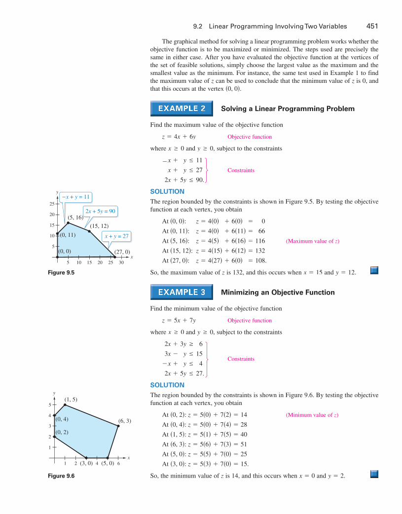
The graphical method for solving a linear programming problem works whether the objective function is to be maximized or minimized. The steps used are precisely the same in either case. After you have evaluated the objective function at the vertices of the set of feasible solutions, simply choose the largest value as the maximum and the smallest value as the minimum. For instance, the same test used in Example 1 to find the maximum value of z can be used to conclude that the minimum value of z is 0, and that this occurs at the vertex (0, 0).
Solving a linear Programming Problem
Find the maximum value of the objective function
z = 4x + 6y Objective function
where x ≥ 0 and y ≥ 0, subject to the constraints
−x +x +
2x +
y ≤ 11
y ≤ 27
5y ≤ 90.
Constraints
SoluTion
The region bounded by the constraints is shown in Figure 9.5. By testing the objective function at each vertex, you obtain
At (0, 0):At (0, 11):At (5, 16):At (15, 12):At (27, 0):
z = 4(0)z = 4(0)z = 4(5)z = 4(15)z = 4(27)
+ 6(0)+ 6(11)+ 6(16)+ 6(12)+ 6(0)
= 0
= 66
= 116
= 132
= 108.
(Maximum value of z)
So, the maximum value of z is 132, and this occurs when x = 15 and y = 12.
minimizing an objective Function
Find the minimum value of the objective function
z = 5x + 7y Objective function
where x ≥ 0 and y ≥ 0, subject to the constraints
2x +3x −
−x +2x +
3y ≥y ≤y ≤
5y ≤
6
15
4
27.
Constraints
SoluTion
The region bounded by the constraints is shown in Figure 9.6. By testing the objective function at each vertex, you obtain
At (0, 2): z = 5(0) + 7(2) = 14 (Minimum value of z)
At (0, 4): z = 5(0) + 7(4) = 28
At (1, 5): z = 5(1) + 7(5) = 40
At (6, 3): z = 5(6) + 7(3) = 51
At (5, 0): z = 5(5) + 7(0) = 25
At (3, 0): z = 5(3) + 7(0) = 15.
So, the minimum value of z is 14, and this occurs when x = 0 and y = 2.
x5
5
10
15
20
25
10 15 20 25 30
(0, 0)
(0, 11)
(5, 16)
(15, 12)
(27, 0)
y
x + y = 27
2x + 5y = 90
−x + y = 11
Figure 9.5
y
x1
1
2
3
4
5
2 4 6
(1, 5)
(0, 4)
(0, 2)
(3, 0) (5, 0)
(6, 3)
Figure 9.6
9781305658004_0902.indd 451 12/3/15 1:58 PM

452 Chapter 9 Linear Programming
When solving a linear programming problem, it is possible that the maximum (or minimum) value occurs at two different vertices. For example, at the vertices of the region shown in Figure 9.7, the objective function
z = 2x + 2y Objective function
has the values below.
At (0, 0): z = 2(0) + 2(0) = 0
At (0, 4): z = 2(0) + 2(4) = 8
At (2, 4): z = 2(2) + 2(4) = 12 (Maximum value of z)
At (5, 1): z = 2(5) + 2(1) = 12 (Maximum value of z)
At (5, 0): z = 2(5) + 2(0) = 10
In this case, the objective function has a maximum value of 12 not only at the vertices (2, 4) and (5, 1), but at any point on the line segment connecting these two vertices.
Some linear programming problems have no optimal solution. This can occur when the region determined by the constraints is unbounded. Example 4 illustrates such a problem.
an unbounded region
See LarsonLinearAlgebra.com for an interactive version of this type of example.
Find the maximum value of
z = 4x + 2y Objective function
where x ≥ 0 and y ≥ 0 subject to the constraints
x +3x +
−x +
2y ≥ 4
y ≥ 7
2y ≤ 7.
Constraints
SoluTion
The region determined by the constraints is shown below.
y
x
1
1 2 53
2
3
4
5
(4, 0)
(2, 1)
(1, 4)
For this unbounded region, there is no maximum value of z. To see this, note that the point (x, 0) lies in the region for all values of x ≥ 4. By choosing large values of x, you can obtain values of
z = 4(x) + 2(0) = 4x
that are large. So, there is no maximum value of z.
x
1
1 2 43
2
3
4(0, 4) (2, 4)
(5, 1)
(5, 0)
(0, 0)
z = 12 for anypoint along
this line.
y
Figure 9.7
remarKFor this problem, the objective function does have a minimum value, z = 10, which occurs at the vertex (2, 1).
9781305658004_0902.indd 452 12/3/15 1:58 PM

9.2 Linear Programming Involving Two Variables 453
aPPlicaTion
an application: optimal cost
Example 4 in Section 9.1 set up a system of linear equations for the problem below. The liquid portion of a diet is to provide at least 300 calories, 36 units of vitamin A, and 90 units of vitamin C daily. A cup of dietary drink X provides 60 calories, 12 units of vitamin A, and 10 units of vitamin C. A cup of dietary drink Y provides 60 calories, 6 units of vitamin A, and 30 units of vitamin C. Now, assume that dietary drink X costs $0.12 per cup and drink Y costs $0.15 per cup. How many cups of each drink should be consumed each day to minimize the cost and still meet the daily requirements?
SoluTion
Begin by letting x be the number of cups of dietary drink X and y be the number of cups of dietary drink Y. Moreover, to meet the minimum daily requirements, the inequalities listed below must be satisfied.
For calories:
For vitamin A:
For vitamin C:
60x +12x +10x +
60y ≥6y ≥
30y ≥x ≥y ≥
300
36
90
0
0
Constraints
The cost C is
C = 0.12x + 0.15y. Objective function
The graph of the region corresponding to the constraints is shown in Figure 9.8. To determine the minimum cost, test C at each vertex of the region, as shown below.
At (0, 6): C = 0.12(0) + 0.15(6) = 0.90
At (1, 4): C = 0.12(1) + 0.15(4) = 0.72
At (3, 2): C = 0.12(3) + 0.15(2) = 0.66 (Minimum value of C)
At (9, 0): C = 0.12(9) + 0.15(0) = 1.08
So, the minimum cost is $0.66 per day, and this occurs when three cups of drink X and two cups of drink Y are consumed each day.
x
2
2 4 6 8 10
4
6
8
10
(0, 6)
(1, 4)
(3, 2)
(9, 0)
y
Figure 9.8
linear algebra aPPlied
When financial institutions replenish automatic teller machines (ATMs), they need to take into account a large number of variables and constraints to keep the machines stocked appropriately. Demand for cash machines fluctuates with such factors as weather, economic conditions, day of the week, and even road construction. Further complicating the matter in the United States is a penalty for depositing and withdrawing money from the Federal Reserve in the same week. To address this complex problem, a company that specializes in providing financial services technology can create high-end optimization software to set up and solve a linear programming problem with many variables and constraints. The company determines an equation for the objective function to minimize total cash in ATMs, while establishing constraints on travel routes, service vehicles, penalty fees, and so on. The optimal solution generated by the software allows the company to build detailed ATM restocking schedules.
Marquis/Shutterstock.com
9781305658004_0902.indd 453 12/3/15 1:58 PM

454 Chapter 9 Linear Programming
9.2 Exercises
Solving a linear Programming Problem In Exercises 1 and 2, find the minimum and maximum values of each objective function and where they occur, subject to the constraints.
1. Objective function: 2. Objective function:
(a) z = 3x + 8y (a) z = 4x + 3y
(b) z = 5x + 0.5y (b) z = x + 6y
Constraints: Constraints:
x +4x +
x ≥y ≥
3y ≤y ≤
00
1516
x ≥y ≥
2x + 3y ≥3x − 2y ≤x + 5y ≤
0069
20
y
x
(0, 5)(3, 4)
(4, 0)(0, 0)
1
1
2
3
4
5
2 3 54
x
(0, 4)(5, 3)
(3, 0)
(0, 2)
1
1
2
3
4
5
2 3 54
y
Solving a linear Programming Problem In Exercises 3–8, sketch the region determined by the constraints. Then find the minimum and maximum values of each objective function (if possible) and where they occur, subject to the constraints.
3. Objective function: 4. Objective function:
(a) z = 10z + 7y (a) z = 50x + 35y
(b) z = 25x + 30y (b) z = 16x + 18y
Constraints: Constraints:
x ≥x ≤y ≥y ≤
5x + 6y ≤
0600
45420
xy
8x + 9y8x + 9y
≥ ≥
≤ ≥
0 0
7200 5400
5. Objective function: 6. Objective function:
(a) z = 4x + 5y (a) z = 4x + 5y
(b) z = 2x − y (b) z = 2x + 7y
(c) z = −5x + y (c) z = −x − 3y
Constraints: Constraints:
x ≥y ≥
2x + 2y ≤x + 2y ≤
00
106 4x +
x +3x +
x ≥y ≥
3y ≥y ≥
5y ≥
00
278
30
7. Objective function: 8. Objective function:
(a) z = x (a) z = 4x + y
(b) z = y (b) z = x + 4y
(c) z = x + y (c) z = 4x + 4y
Constraints: Constraints:
x ≥y ≥
2x + 3y ≤2x + y ≤4x + y ≤
00
602848
x ≥y ≥
x + 2y ≤x + y ≥
2x + 3y ≥
00
403072
Finding minimum and maximum values In Exercises 9–14, find the minimum and maximum values of the objective function and the points (x1, x2) where they occur, subject to the constraints 3x1 + x2 ≤ 15 and 4x1 + 3x2 ≤ 30, where x1, x2 ≥ 0.
9. z = 2x1 + x2 10. z = 5x1 + x2
11. z = x1 + x2 12. z = 3x1 + x2
13. z = x1 + 5x2 14. z = 4x1 + 5x2
describing an unusual characteristic In Exercises 15–20, the linear programming problem has an unusual characteristic. Sketch a graph of the solution region for the problem and describe the unusual characteristic. (In each problem, the objective function is to be maximized.)
15. Objective function: 16. Objective function:
z = 2.5x + y z = x + y
Constraints: Constraints:
x ≥y ≥
3x + 5y ≤5x + 2y ≤
00
1510
x ≥y ≥
−x + y ≤−x + 2y ≤
0014
17. Objective function: 18. Objective function:
z = −x + 2y z = x + y
Constraints: Constraints:
x ≥y ≥x ≤
x + y ≤
00
107
x ≥y ≥
−x + y ≤−3x + y ≥
0003
19. Objective function: 20. Objective function:
z = 3x + 4y z = x + 2y
Constraints: Constraints:
x ≥y ≥
x + y ≤2x + y ≥
0014
x ≥y ≥
x + 2y ≤2x + y ≥
0044
9781305658004_0902.indd 454 12/3/15 1:59 PM

9.2 Exercises 455
21. optimal Profit The costs to a store for two models of Global Positioning System (GPS) receivers are $80 and $100. The $80 model yields a profit of $25 and the $100 model yields a profit of $30. Market tests and available resources determined the constraints below.
(a) The merchant estimates that the total monthly demand will not exceed 200 units.
(b) The merchant does not want to invest more than $18,000 in GPS receiver inventory.
What is the optimal inventory level for each model? What is the optimal profit?
22. optimal Profit A fruit grower has 150 acres of land for raising crops A and B. The profit is $185 per acre for crop A and $245 per acre for crop B. Research and available resources determined the constraints below.
(a) It takes 1 day to trim an acre of crop A and 2 days to trim an acre of crop B, and there are 240 days per year available for trimming.
(b) It takes 0.3 day to pick an acre of crop A and 0.1 day to pick an acre of crop B, and there are 30 days per year available for picking.
What is the optimal acreage for each fruit? What is the optimal profit?
23. optimal cost A farming cooperative mixes two brands of cattle feed. Brand X costs $30 per bag, and brand Y costs $25 per bag. Research and available resources determined the constraints below.
(a) Brand X contains two units of nutritional element A, two units of element B, and two units of element C.
(b) Brand Y contains one unit of nutritional element A, nine units of element B, and three units of element C.
(c) The minimum requirements for nutrients A, B, and C are 12 units, 36 units, and 24 units, respectively.
What is the optimal number of bags of each brand that should be mixed? What is the optimal cost?
24. optimal cost Rework Exercise 23 assuming that brand Y now costs $32 per bag, and it now contains one unit of nutritional element A, twelve units of element B, and four units of element C.
25. optimal revenue An accounting firm charges $2500 for an audit and $350 for a tax return. The table shows the times (in hours) required for staffing and reviewing.
Component Audit Tax Return
Staffing 75 12.5
Reviewing 10 2.5
The firm has 900 hours of staff time and 155 hours of review time available each week. What numbers of audits and tax returns will bring in an optimal revenue?
26. optimal revenue The accounting firm in Exercise 25 lowers its charge for an audit to $2000. What numbers of audits and tax returns will bring in an optimal revenue?
27. Determine, for each vertex, values of t such that the objective function has a maximum value at the vertex (if possible).
Objective function:
z = 3x + ty
Constraints:
x ≥y ≥
7x + 14y ≤5x + 4y ≤
00
8430
(a) (0, 6) (b) (2, 5) (c) (6, 0) (d) (0, 0)
28. CAPSTONE A company determining an optimal profit finds that the objective function has a maximum value at the vertices shown in the graph.
x
y
(5, 7)
(0, 12)
2 4 6 8 10
2
4
6
8
10
12
14
(a) Can you conclude that it also has a maximum value at the point (3, 9)? Explain.
(b) Can you conclude that it also has a maximum value at the point (6, 6)? Explain.
(c) Find two additional points that maximize the objective function.
Finding an objective Function In Exercises 29–32, find an objective function that has a maximum or minimum value at the specified vertex of the constraint region shown below. (There are many correct answers.)
29. Maximum at vertex A
1 2 3 4 5 6
123
56
A(0, 4)B(4, 3)
C(5, 0)x
y
30. Maximum at vertex B
31. Maximum at vertex C
32. Minimum at vertex C
9781305658004_0902.indd 455 12/3/15 1:59 PM
456 Chapter 9 Linear Programming
9.3 The Simplex Method: Maximization
Write the simplex tableau for a linear programming problem.
Use pivoting to find an improved solution.
Use the simplex method to solve a linear programming problem that maximizes an objective function.
Use the simplex method to find an optimal solution to a real-world application.
The Simplex Tableau
For linear programming problems involving two variables, the graphical solution method introduced in Section 9.2 is convenient. For problems involving more than two variables or large numbers of constraints, it is better to use methods that are adaptable to technology. One such method is the simplex method, developed by George Dantzig in 1946. It provides a systematic way of examining the vertices of the feasible region to determine the optimal value of the objective function.
Say you want to find the maximum value of z = 4x1 + 6x2, where the decision variables x1 and x2 are nonnegative, subject to the constraints
−x1 +x1 +
2x1 +
x2 ≤ 11
x2 ≤ 27
5x2 ≤ 90.
The left-hand side of each inequality is less than or equal to the right-hand side, so there must exist nonnegative numbers s1, s2, and s3 that can be added to the left side of each equation to produce the system of linear equations
−x1 +x1 +
2x1 +
x2
x2
5x2
+ s1
+ s2
= 11
= 27
+ s3 = 90.
The numbers s1, s2, and s3 are called slack variables because they represent the “slack” in each inequality.
Standard Form of a linear programming problem
A linear programming problem is in standard form when it seeks to maximize the objective function z = c1x1 + c2x2 + . . . + cnxn subject to the constraints
a11x1 +a21x1 +
am1x1 +
a12x2 +a22x2 +
am2x2 +
. . . +
. . . +
. . . +
a1nxn ≤a2nxn ≤
⋮
amnxn ≤
b1
b2
bm
where xi ≥ 0 and bi ≥ 0. After adding slack variables, the corresponding system of constraint equations is
a11x1 +a21x1 +
am1x1 +
a12x2 + . . . +a22x2 + . . . +
am2x2 + . . . +
a1nxn
a2nxn
amnxn
+ s1
+ s2
==
⋮
+ sm =
b1
b2
bm
where si ≥ 0.
RemaRKNote that for a linear programming problem in standard form, the objective function is to be maximized, not minimized. (Minimization problems are discussed in Sections 9.4 and 9.5.)
9781305658004_0903.indd 456 12/3/15 2:00 PM

9.3 The Simplex Method: Maximization 457
A basic solution of a linear programming problem in standard form is a solution (x1, x2, . . . , xn, s1, s2, . . . , sm) of the constraint equations in which at most m variables are nonzero, and the variables that are nonzero are called basic variables. A basic solution for which all variables are nonnegative is a basic feasible solution.
The simplex method is carried out by performing elementary row operations on a matrix called the simplex tableau. This tableau consists of the augmented matrix corresponding to the constraint equations together with the coefficients of the objective function written in the form
−c1x1 − c2x2 − . . . − cnxn + (0)s1 + (0)s2 + . . . + (0)sm + z = 0.
In the tableau, it is customary to omit the coefficient of z. For example, the simplex tableau for the linear programming problem
z = 4x1 + 6x2 Objective function
−x1 +x1 +
2x1 +
x2
x2
5x2
+ s1
+ s2
= 11
= 27
+ s3 = 90
Constraints
is shown below.
x1 x2 s1 s2 s3 bBasic
Variables
−1 1 1 0 0 11 s1
1 1 0 1 0 27 s2
2 5 0 0 1 90 s3
−4 −6 0 0 0 0
→
Current z-value
For this initial simplex tableau, the basic variables are s1, s2, and s3, and the nonbasic variables are x1 and x2. Note that the basic variables are labeled to the right of the simplex tableau next to the appropriate rows. This technique is important as you proceed through the simplex method. It helps keep track of the changing basic variables, as shown in Example 1.
x1 and x2 are the nonbasic variables in this initial tableau, so they have an initial value of zero, yielding a current z-value of zero. From the columns that are farthest to the right, the basic variables have initial values of s1 = 11, s2 = 27, and s3 = 90. So the current solution is
x1 = 0
x2 = 0
s1 = 11
s2 = 27
s3 = 90.
This solution is a basic feasible solution and is often written as
(x1, x2, s1, s2, s3) = (0, 0, 11, 27, 90).
The entry in the lower right corner of the simplex tableau is the current value of z. Note that the bottom-row entries under x1 and x2 are the negatives of the coefficients of x1 and x2 in the objective function
z = 4x1 + 6x2.
To perform an optimality check for a solution represented by a simplex tableau, look at the entries in the bottom row of the tableau. If any of these entries are negative (as above), then the current solution is not optimal.
9781305658004_0903.indd 457 12/3/15 2:01 PM

458 Chapter 9 Linear Programming
pivoTing
After you have set up the initial simplex tableau for a linear programming problem, the simplex method consists of checking for optimality and then, when the current solution is not optimal, improving the current solution. (An improved solution is one that has a larger z-value than the current solution.) To improve the current solution, bring a new basic variable into the solution, the entering variable. This implies that one of the current basic variables (the departing variable) must leave, otherwise you would have too many variables for a basic solution. Choose the entering and departing variables as listed below.
1. The entering variable corresponds to the least (the most negative) entry in the bottom row of the tableau, excluding the “b-column.”
2. The departing variable corresponds to the least nonnegative ratio bi�aij in the column determined by the entering variable, when aij > 0.
3. The entry in the simplex tableau in the entering variable’s column and the departing variable’s row is the pivot.
Finally, to form the improved solution, apply Gauss-Jordan elimination to the column that contains the pivot, as illustrated in Example 1. (This process is called pivoting.)
pivoting to Find an improved Solution
Use the simplex method to find an improved solution for the linear programming problem represented by the tableau shown below.
x1 x2 s1 s2 s3 bBasic
Variables
−1 1 1 0 0 11 s1
1 1 0 1 0 27 s2
2 5 0 0 1 90 s3
−4 −6 0 0 0 0
SoluTion
The objective function for this problem is
z = 4x1 + 6x2.
Note that the current solution
(x1 = 0, x2 = 0, s1 = 11, s2 = 27, s3 = 90)
corresponds to a z-value of 0. To improve this solution, choose x2 as the entering variable, because −6 is the least entry in the bottom row.
x1 x2 s1 s2 s3 bBasic
Variables
−1 1 1 0 0 11 s1
1 1 0 1 0 27 s2
2 5 0 0 1 90 s3
−4 −6 0 0 0 0
→
Entering
To see why you choose x2 as the entering variable, remember that z = 4x1 + 6x2. So, it appears that a unit change in x2 produces a change of 6 in z, whereas a unit change in x1 produces a change of only 4 in z.
9781305658004_0903.indd 458 12/3/15 2:01 PM

9.3 The Simplex Method: Maximization 459
To find the departing variable, locate the bi’s that have corresponding positive elements in the entering variable’s column and form the ratios
111
= 11, 271
= 27, and 905
= 18.
Here the least nonnegative ratio is 11, so choose s1 as the departing variable.
x1 x2 s1 s2 s3 bBasic
Variables
−1 1 1 0 0 11 s1
1 1 0 1 0 27 s2
2 5 0 0 1 90 s3
−4 −6 0 0 0 0
→
Entering
Note that the pivot is the entry in the first row and second column. Now, use Gauss-Jordan elimination to obtain the improved solution shown below.
Before Pivoting After Pivoting
[−1
12
−4
115
−6
1000
0100
0010
1127900] [
−127
−10
1000
1−1−5
6
0100
0010
11163566
] −R1 + R2
−5R1 + R3
6R1 + R4
The new tableau is shown below.
x1 x2 s1 s2 s3 bBasic
Variables
−1 1 1 0 0 11 x2
2 0 −1 1 0 16 s2
7 0 −5 0 1 35 s3
−10 0 6 0 0 66
Note that x2 has replaced s1 in the basic variables column and the improved solution
(x1, x2, s1, s2, s3) = (0, 11, 0, 16, 35)
has a z-value of
z = 4x1 + 6x2 = 4(0) + 6(11) = 66.
In Example 1, the improved solution is not optimal because the bottom row has a negative entry. So, apply another iteration of the simplex method to improve the solution further. Choose x1 as the entering variable. Moreover, the lesser of the ratios 16�2 = 8 and 35�7 = 5 is 5, so s3 is the departing variable. Gauss-Jordan elimination produces the matrices shown below.
[−1
27
−10
1000
1−1−5
6
0100
0010
11163566
] [−1
21
−10
1000
1−1−5
7
6
0100
0017
0
11165
66] 1
7R3
[001
−10
1000
2737
−57
−87
0100
172717
107
1665
116]
R1 + R3
R2 − 2R3
R4 + 10R3
RemaRKIn the event of a tie when choosing entering and/or departing variables, any of the tied variables may be chosen.
→ Departing
9781305658004_0903.indd 459 12/3/15 2:01 PM

460 Chapter 9 Linear Programming
So, the new simplex tableau is as shown below.
x1 x2 s1 s2 s3 bBasic
Variables
0 1 27 0 1
7 16 x2
0 0 37 1 −2
7 6 s2
1 0 −57 0 1
7 5 x1
0 0 −87 0 10
7 116
In this tableau, there is still a negative entry in the bottom row. So, choose s1 as the entering variable and s2 as the departing variable, as shown in the next tableau.
x1 x2 s1 s2 s3 bBasic
Variables
0 1 27 0 1
7 16 x2
0 0 37 1 −2
7 6 s2
1 0 −57 0 1
7 5 x1
0 0 −87 0 10
7 116
→
Entering
One more iteration of the simplex method gives the tableau below. (Check this.)
x1 x2 s1 s2 s3 bBasic
Variables
0 1 0 −23
13 12 x2
0 0 1 73 −2
3 14 s1
1 0 0 53 −1
3 15 x1
0 0 0 83
23 132
In this tableau, there are no negative elements in the bottom row. So, the optimal solution is
(x1, x2, s1, s2, s3) = (15, 12, 14, 0, 0)
with
z = 4x1 + 6x2 = 4(15) + 6(12) = 132.
The linear programming problem in Example 1 involved only two decision variables, x1 and x2, so you could have used a graphical solution technique, as in Section 9.2, Example 2. Notice in the figure below that each iteration in the simplex method corresponds to moving from one vertex to an adjacent vertex with an improved z-value.
(0, 0) (0, 11) (5, 16) (15, 12) z = 0 z = 66 z = 116 z = 132
x1
x2
5
5
10
15
20
25
10 15 20 25 30
(0, 0)
(0, 11)
(5, 16)
(15, 12)
(27, 0)
→ Departing
→ Maximum z-value
9781305658004_0903.indd 460 12/3/15 2:01 PM

9.3 The Simplex Method: Maximization 461
The Simplex meThod
Here is a summary of the steps involved in the simplex method.
Note that the basic feasible solution of an initial simplex tableau is
(x1, x2, . . . , xn, s1, s2, . . . , sm) = (0, 0, . . . , 0, b1, b2, . . . , bm).
This solution is basic because at most m variables are nonzero (namely, the slack variables). It is feasible because each variable is nonnegative.
The next two examples illustrate the use of the simplex method to solve a problem involving three decision variables.
The Simplex method (Standard Form)
To solve a linear programming problem in standard form, use the steps below.
1. Convert each inequality in the set of constraints to an equation by adding slack variables.
2. Create the initial simplex tableau.3. Locate the most negative entry in the bottom row, excluding the “b-column.”
This entry is called the entering variable, and its column is the entering column. (If ties occur, then any of the tied entries can be used to determine the entering column.)
4. Form the ratios of the entries in the “b-column” with their corresponding positive entries in the entering column. (If all entries in the entering column are 0 or negative, then there is no maximum solution.) The departing row corresponds to the least nonnegative ratio bi�aij. (For ties, choose any corresponding row.) The entry in the departing row and the entering column is called the pivot.
5. Use elementary row operations to change the pivot to 1 and all other entries in the entering column to 0. This process is called pivoting.
6. When all entries in the bottom row are zero or positive, this is the final tableau. Otherwise, go back to Step 3.
7. If you obtain a final tableau, then the linear programming problem has a maximum solution. The maximum value of the objective function is the entry in the lower right corner of the tableau.
lineaR algebRa applied
There are many commercially available optimization software packages to aid operations researchers in such areas as allocating resources to maximize profits and minimize costs. Many of these packages use the simplex method as their foundation. Also, free online tools are available that enable you to check your work in this chapter. Many of these are user-friendly interfaces that use the simplex method as well as the graphical method to solve linear programming problems. These freeware programs show the steps in the solution, which can be very helpful in the learning process. Use online optimization freeware to check the solution of Example 1 in this section and to check the solution of Example 2 in Section 9.2. As you will see in the next section, the simplex method can also be applied to minimization problems. In addition to optimizing the objective function, commercially available software packages often contain built-in sensitivity reporting to analyze how changes or errors in the data will affect the outcome.
Marcin Balcerzak/Shutterstock.com
9781305658004_0903.indd 461 12/3/15 2:01 PM

462 Chapter 9 Linear Programming
The Simplex method with Three decision variables
See LarsonLinearAlgebra.com for an interactive version of this type of example.
Use the simplex method to find the maximum value of
z = 2x1 − x2 + 2x3 Objective function
subject to the constraints
2x1 +x1 +
x2
2x2
x2
≤− 2x3 ≤+ 2x3 ≤
10
20
5
where x1 ≥ 0, x2 ≥ 0, and x3 ≥ 0.
SoluTion
Using the basic feasible solution
(x1, x2, x3, s1, s2, s3) = (0, 0, 0, 10, 20, 5)
the initial and subsequent simplex tableaus for this problem are shown below. (Check the computations, and note the “tie” that occurs when choosing the first entering variable.)
x1 x2 x3 s1 s2 s3 bBasic
Variables
2 1 0 1 0 0 10 s1
1 2 −2 0 1 0 20 s2
0 1 2 0 0 1 5 s3
−2 1 −2 0 0 0 0
→
Entering
x1 x2 x3 s1 s2 s3 bBasic
Variables
2 1 0 1 0 0 10 s1
1 3 0 0 1 1 25 s2
0 12 1 0 0 1
252 x3
−2 2 0 0 0 1 5
→
Entering
x1 x2 x3 s1 s2 s3 bBasic
Variables
1 12 0 1
2 0 0 5 x1
0 52 0 −1
2 1 1 20 s2
0 12 1 0 0 1
252 x3
0 3 0 1 0 1 15
This implies that the optimal solution is
(x1, x2, x3, s1, s2, s3) = (5, 0, 52, 0, 20, 0)and the maximum value of z is 15.
Note that s2 = 20. The optimal solution yields a maximum value of z = 15 provided that x1 = 5, x2 = 0, and x3 = 5
2. Check that these values satisfy the constraints giving equality in the first and third constraints, yet the second constraint has a slack of 20.
→ Departing
→ Departing
9781305658004_0903.indd 462 12/3/15 2:01 PM

9.3 The Simplex Method: Maximization 463
Occasionally, the constraints in a linear programming problem will include an equation. In such cases, add a “slack variable” called an artificial variable to form the initial simplex tableau. Technically, this new variable is not a slack variable (because there is no slack to be taken). Once you have determined an optimal solution in such a problem, check that any equations in the original constraints are satisfied. Example 3 illustrates such a case.
The Simplex method with Three decision variables
Use the simplex method to find the maximum value of
z = 3x1 + 2x2 + x3 Objective function
subject to the constraints
4x1 +2x1 +x1 +
x2 +3x2 +2x2 +
x3 = 30
x3 ≤ 60
3x3 ≤ 40
where x1 ≥ 0, x2 ≥ 0, and x3 ≥ 0.
SoluTion
Using the basic feasible solution (x1, x2, x3, s1, s2, s3) = (0, 0, 0, 30, 60, 40), the initial and subsequent simplex tableaus for this problem are shown below. (Note that s1 is an artificial variable, rather than a slack variable.)
x1 x2 x3 s1 s2 s3 bBasic
Variables
4 1 1 1 0 0 30 s1
2 3 1 0 1 0 60 s2
1 2 3 0 0 1 40 s3
−3 −2 −1 0 0 0 0
→
Entering
x1 x2 x3 s1 s2 s3 bBasic
Variables
1 14
14
14 0 0 15
2 x1
0 52
12 −1
2 1 0 45 s2
074
114 −1
4 0 1 652 s3
0 −54 −1
434
0 0 452
→
Entering
x1 x2 x3 s1 s2 s3 bBasic
Variables
1 0 15
310 − 1
10 0 3 x1
0 1 15 −1
525 0 18 x2
0 0 125
110 − 7
10 1 1 s3
0 0 0 12
12
0 45
So the optimal solution is (x1, x2, x3, s1, s2, s3) = (3, 18, 0, 0, 0, 1) and the maximum value of z is 45. This solution satisfies the equation provided in the constraints, because 4(3) + 1(18) + 1(0) = 30.
→ Departing
→ Departing
9781305658004_0903.indd 463 12/3/15 2:01 PM
464 Chapter 9 Linear Programming
applicaTionS
Example 4 shows how to use the simplex method to maximize profits in a business application.
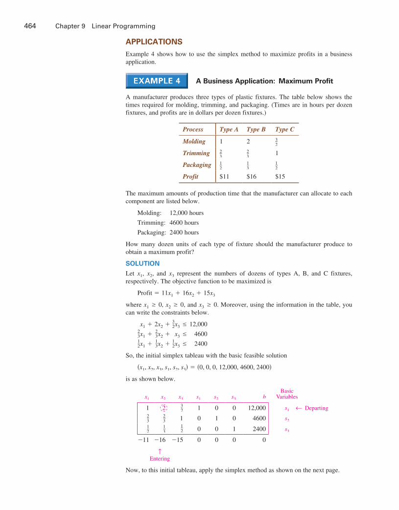
a business application: maximum profit
A manufacturer produces three types of plastic fixtures. The table below shows the times required for molding, trimming, and packaging. (Times are in hours per dozen fixtures, and profits are in dollars per dozen fixtures.)
The maximum amounts of production time that the manufacturer can allocate to each component are listed below.
Molding: 12,000 hours
Trimming: 4600 hours
Packaging: 2400 hours
How many dozen units of each type of fixture should the manufacturer produce to obtain a maximum profit?
SoluTion
Let x1, x2, and x3 represent the numbers of dozens of types A, B, and C fixtures, respectively. The objective function to be maximized is
Profit = 11x1 + 16x2 + 15x3
where x1 ≥ 0, x2 ≥ 0, and x3 ≥ 0. Moreover, using the information in the table, you can write the constraints below.
x1 +23x1 +12x1 +
2x2 +23x2 +13x2 +
32x3 ≤x3 ≤
12x3 ≤
12,000
4600
2400
So, the initial simplex tableau with the basic feasible solution
(x1, x2, x3, s1, s2, s3) = (0, 0, 0, 12,000, 4600, 2400)
is as shown below.
x1 x2 x3 s1 s2 s3 bBasic
Variables
1 2 32 1 0 0 12,000 s1
23
23 1 0 1 0 4600 s2
12
13
12 0 0 1 2400 s3
−11 −16 −15 0 0 0 0
→
Entering
Now, to this initial tableau, apply the simplex method as shown on the next page.
Process Type A Type B Type C
Molding 1 2 32
Trimming 23
23
1
Packaging 12
13
12
Profit $11 $16 $15
→ Departing
9781305658004_0903.indd 464 12/3/15 2:01 PM
9.3 The Simplex Method: Maximization 465
x1 x2 x3 s1 s2 s3 bBasic
Variables
12 1 3
412 0 0 6000 x2
13 0 1
2 −13 1 0 600 s2
13 0 1
4 −16 0 1 400 s3
−3 0 −3 8 0 0 96,000
→
Entering
x1 x2 x3 s1 s2 s3 bBasic
Variables
0 1 38
34 0 −3
2 5400 x2
0 0 14 −1
6 1 −1 200 s2
1 0 34 −1
2 0 3 1200 x1
0 0 −34
132 0 9 99,600
→
Entering
x1 x2 x3 s1 s2 s3 bBasic
Variables
0 1 0 1 −32 0 5100 x2
0 0 1 −23 4 −4 800 x3
1 0 0 0 −3 6 600 x1
0 0 0 6 3 6 100,200
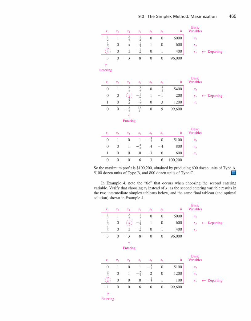
So the maximum profit is $100,200, obtained by producing 600 dozen units of Type A, 5100 dozen units of Type B, and 800 dozen units of Type C.
In Example 4, note the “tie” that occurs when choosing the second entering variable. Verify that choosing x3 instead of x1 as the second entering variable results in the two intermediate simplex tableaus below, and the same final tableau (and optimal solution) shown in Example 4.
x1 x2 x3 s1 s2 s3 bBasic
Variables
12 1 3
412 0 0 6000 x2
13 0 1
2 −13 1 0 600 s2
13 0 1
4 −16 0 1 400 s3
−3 0 −3 8 0 0 96,000
→
Entering
x1 x2 x3 s1 s2 s3 bBasic
Variables
0 1 0 1 −32 0 5100 x2
23 0 1 −2
3 2 0 1200 x3
16 0 0 0 −1
2 1 100 s3
−1 0 0 6 6 0 99,600
→
Entering
→ Departing
→ Departing
→ Departing
→ Departing
9781305658004_0903.indd 465 12/3/15 2:01 PM

466 Chapter 9 Linear Programming
Example 5 shows how to use the simplex method to maximize the audience in an advertising campaign.
a business application: media Selection
Advertising alternatives for a company include television, radio, and newspaper. The table below shows the costs and estimates of audience coverage for each type of media.
Cost per advertisement
Audience per advertisement
Television $2000 100,000
Newspaper $600 40,000
Radio $300 18,000
The newspaper limits the number of weekly advertisements from a single company to ten. Moreover, to balance the advertising among the three types of media, no more than half of the total number of advertisements should occur on the radio, and at least 10% should occur on television. The weekly advertising budget is $18,200. How many advertisements should run in each of the three types of media to maximize the total audience?
SoluTion
Let x1, x2, and x3 represent the numbers of advertisements on television, in the newspaper, and on the radio, respectively. The objective function to be maximized is
z = 100,000x1 + 40,000x2 + 18,000x3 Objective function
where x1 ≥ 0, x2 ≥ 0, and x3 ≥ 0. The constraints for this problem are shown below.
2000x1
x1
+ 600x2
x2
+ 300x3 ≤≤
x3 ≤≥
18,200 10
0.5(x1 + x2 + x3)0.1(x1 + x2 + x3)
Here is a more manageable form of this system of constraints.
20x1 +
−x1 −−9x1 +
6x2
x2
x2
x2
+
++
3x3 ≤≤
x3 ≤x3 ≤
1821000
Constraints
So, the initial simplex tableau is below.
x1 x2 x3 s1 s2 s3 s4 bBasic
Variables
20 6 3 1 0 0 0 182 s1
0 1 0 0 1 0 0 10 s2
−1 −1 1 0 0 1 0 0 s3
−9 1 1 0 0 0 1 0 s4
−100,000 −40,000 −18,000 0 0 0 0 0
→
Entering
→Departing
9781305658004_0903.indd 466 12/3/15 2:01 PM

9.3 The Simplex Method: Maximization 467
Now, to this initial tableau, apply the simplex method, as shown below.
x1 x2 x3 s1 s2 s3 s4 bBasic
Variables
1 310
320
120 0 0 0 91
10 x1
0 1 0 0 1 0 0 10 s2
0 − 710
2320
120 0 1 0 91
10 s3
0 3710
4720
920 0 0 1 819
10 s4
0 −10,000 −3000 5000 0 0 0 910,000
→
Entering
x1 x2 x3 s1 s2 s3 s4 bBasic
Variables
1 0 320
120 − 3
10 0 0 6110 x1
0 1 0 0 1 0 0 10 x2
0 0 2320
120
710 1 0 161
10 s3
0 0 4720
920 −37
10 0 1 44910 s4
0 0 −3000 5000 10,000 0 0 1,010,000
→
Entering
x1 x2 x3 s1 s2 s3 s4 bBasic
Variables
1 0 0 123 − 9
23 − 323 0 4 x1
0 1 0 0 1 0 0 10 x2
0 0 1 123
1423
2023 0 14 x3
0 0 0 823 −118
23 −4723 1 12 s4
0 0 0 118,00023
272,00023
60,00023
0 1,052,000
From this final simplex tableau, the maximum weekly audience for an advertising budget of $18,200 is
z = 1,052,000 Maximum weekly audience
which occurs when
x1 =x2 =x3 =
4
10
14.
The table below summarizes the results.
Media
Number of advertisements
Cost
Audience
Television 4 $8000 400,000
Newspaper 10 $6000 400,000
Radio 14 $4200 252,000
Total 28 $18,200 1,052,000
→ Departing
→ Departing
9781305658004_0903.indd 467 12/3/15 2:01 PM

468 Chapter 9 Linear Programming
9.3 Exercises
Standard Form In Exercises 1–4, explain why the linear programming problem is not in standard form.
1. (Minimize) 2. (Maximize) Objective function: Objective function:
z = x1 + x2 z = x1 + x2
Constraints: Constraints:
x1 + 2x2 ≤ 4
x1, x2 ≥ 0
x1 +2x1 −
2x2 ≤x2 ≤
6−1
x1, x2 ≥ 0
3. (Maximize) 4. (Maximize) Objective function: Objective function:
z = x1 + x2 z = x1 + x2
Constraints: Constraints:
x1
2x1
+ x2 +−
3x3 ≤ 52x3 ≥ 1
x1 + x2 ≥ 4
2x1 + x2 ≥ 6 x1, x2, x3 ≥ 0 x1, x2 ≥ 0
Writing a Simplex Tableau In Exercises 5–8, write the simplex tableau for the linear programming problem. You do not need to solve the problem.
5. (Maximize) 6. (Maximize) Objective function: Objective function:
z = x1 + 2x2 z = x1 + 3x2
Constraints: Constraints:
2x1 + x2 ≤x1 + x2 ≤
x1, x2 ≥
850
x1 + x2 ≤x1 − x2 ≤
x1, x2 ≥
410
7. (Maximize) 8. (Maximize) Objective function: Objective function:
z = 2x1 + 3x2 + 4x3 z = 6x1 − 9x2
Constraints: Constraints:
x1
x1
+ 2x2 ≤+ x3 ≤
128
2x1 −x1 +
3x2 ≤x2 ≤
620
x1, x2, x3 ≥ 0 x1, x2 ≥ 0
pivoting to Find an improved Solution In Exercises 9 and 10, use one iteration of pivoting to find an improved solution for the linear programming problem represented by the tableau.
9. x1 x2 s1 s2 s3 b
BasicVariables
−10 3 1 0 0 32 s1
2 −2 0 1 0 16 s2
3 12 0 0 1 28 s3
−5 −2 0 0 0 0
10. x1 x2 s1 s2 s3 b
BasicVariables
9 15 1 0 0 750 s1
15 −10 0 1 0 60 s2
−12 50 0 0 1 3000 s3
−45 −78 0 0 0 0
using the Simplex method In Exercises 11–24, use the simplex method to maximize the objective function, subject to the constraints.
11. Objective function: 12. Objective function:
z = x1 + 2x2 z = x1 + x2
Constraints: Constraints:
x1 +x1 +
4x2 ≤x2 ≤
812
x1 + 2x2 ≤
3x1 + 2x1 ≤6
12 x1, x2 ≥ 0 x1, x2 ≥ 0
13. Objective function: 14. Objective function:
z = 3x1 + 2x2 z = 4x1 + 5x2
Constraints: Constraints:
x1 +
4x1 +3x2 ≤ 15x2 ≤ 16
2x1 + 2x2 ≤x1 + 2x2 ≤
106
x1, x2 ≥ 0 x1, x2 ≥ 0
15. Objective function: 16. Objective function:
z = 10x1 + 7x2 z = 25x1 + 35x2
Constraints: Constraints:
x1 ≤x2 ≤
5x1 + 6x2 ≤
6045
420
18x1 + 9x2 ≤ 72008x1 + 9x2 ≤ 3600
x1, x2 ≥ 0 x1, x2 ≥ 0
17. Objective function: 18. Objective function:
z = 4x1 + 5x2 z = x1 + 2x2
Constraints: Constraints:
x1 +
3x1 +−3x1 +
x2 ≤ 107x2 ≤ 427x2 ≤ 28
x1 +
2x1 −−4x1 +
3x2 ≤x2 ≤
3x2 ≤
15120
x1, x2 ≥ 0 x1, x2 ≥ 0
19. Objective function: 20. Objective function:
z = 5x1 + 2x2 + 8x3 z = x1 − x2 + 2x3
Constraints: Constraints:
2x1 −2x1 +6x1 −
4x2 +3x2 −x2 +
x3 ≤ 42x3 ≤ 42
3x3 ≤ 42
2x1 + 2x2 ≤x3 ≤
x1, x2, x3 ≥
850
x1, x2, x3 ≥ 0
9781305658004_0903.indd 468 12/3/15 2:01 PM

9.3 Exercises 469
21. Objective function:
z = x1 − x2 + x3
Constraints:
2x1
x1
+ x2 −+
2x2 +
3x3 ≤ 40x3 ≤ 25
3x3 ≤ 32 x1, x2, x3 ≥ 0
22. Objective function:
z = 3x1 + 4x2 + x3 + 7x4
Constraints:
8x1 + 3x2 +2x1 + 6x2 +x1 + 4x2 +
4x3 +x3 +
5x3 +
x4 ≤ 75x4 ≤ 32x4 ≤ 8
x1, x2, x3, x4 ≥ 0
23. Objective function:
z = x1 + 2x2 − x4
Constraints:
x1 + 2x2 + 3x3
3x2 + 7x3
≤ 24+ x4 ≤ 42
x1, x2, x3, x4 ≥ 0
24. Objective function:
z = x1 + 2x2 + x3 − x4
Constraints:
x1
2x1
4x1
+
+
x2
x2
3x2
++
−
3x3 + 4x4 ≤ 602x3 + 5x4 ≤ 50
+ 6x4 ≤ 72x3 + 3x4 ≤ 48
x1, x2, x3, x4 ≥ 0
using artificial variables In Exercises 25 and 26, use an artificial variable to solve the linear programming problem, and check your solution.
25. Objective function:
z = 10x1 + 5x2 + 12x3
Constraints:
−2x1
x1
+
−
x2 +−
x2 +
2x3 ≤ 80x3 = 35
3x3 ≤ 60 x1, x2, x3 ≥ 0
26. Objective function:
z = 9x1 + x2 + 2x3
Constraints:
2x1
4x1
−2x1
+ 6x2
− 3x2
++
=2x3 ≤x3 ≤
82112
x1, x2, x3 ≥ 0
27. optimal Revenue An accounting firm charges $2000 for an audit and $300 for a tax return. The table shows the times (in hours) required for staffing and reviewing.
Component Audit Tax Return
Staffing 100 12.5
Reviewing 10 2.5
The firm has 900 hours of staff time and 100 hours of review time available each week. Use the simplex method to find the numbers of audits and tax returns that will bring in a maximum revenue.
28. optimal Revenue The accounting firm in Exercise 27 raises its charge for an audit to $2500. Use the simplex method to find the numbers of audits and tax returns that will bring in a maximum revenue.
29. optimal profit A fruit juice company makes two special drinks by blending apple and pineapple juices. The profit per liter is $0.60 for the first drink and $0.50 for the second drink. The table shows the portions of apple and pineapple juice in each drink.
Ingredient First drink Second drink
Apple juice 30% 60%
Pineapple juice 70% 40%
There are 1000 liters of apple juice and 1500 liters of pineapple juice available. Use the simplex method to find the numbers of liters of each drink that should be produced in order to maximize the profit.
30. optimal profit Rework Exercise 29 assuming that the second drink was changed to contain 80% apple juice and 20% pineapple juice.
31. optimal profit A manufacturer produces three models of bicycles. The table shows the times (in hours) required for assembling, painting, and packaging each model.
Model A Model B Model C
Assembling 2 2.5 3
Painting 1.5 2 1
Packaging 1 0.75 1.25
The total times available for assembling, painting, and packaging are 4006 hours, 2495 hours, and 1500 hours, respectively. The profits per unit are $45 for model A, $50 for model B, and $55 for model C. What is the optimal production level for each model? What is the optimal profit?
9781305658004_0903.indd 469 12/3/15 2:01 PM

470 Chapter 9 Linear Programming
32. optimal profit Rework Exercise 31 assuming that the total times available for assembling, painting, and packaging are 4000 hours, 2500 hours, and 1500 hours, respectively, and that the profits per unit are $48 for model A, $50 for model B, and $52 for model C.
33. optimal profit A grower raises crops X, Y, and Z. The profit is $60 per acre for crop X, $20 per acre for crop Y, and $30 per acre for crop Z. Research and available resources determined the constraints below.
(a) The grower has 50 acres of land available.
(b) The costs per acre of producing crops X, Y, and Z are $200, $80, and $140, respectively.
(c) The grower’s total cost cannot exceed $10,000.
Use the simplex method to find the optimal number of acres of land for each crop. What is the maximum profit?
34. investment An investor has up to $450,000 to invest in three types of investments. Type A investments pay 6% annually and have a risk factor of 0. Type B investments pay 10% annually and have a risk factor of 0.06. Type C investments pay 12% annually and have a risk factor of 0.08. To have a well-balanced portfolio, the investor imposes some conditions. The average risk factor should be no greater than 0.05. Moreover, at least one-half of the total portfolio is to be allocated to type A investments and at least one-fourth of the portfolio is to be allocated to type B investments. How much should the investor allocate to each type of investment to obtain a maximum return?
35. Use the simplex method to find the value(s) of t such that the objective function z = 2x1 − tx2 + x3 has a maximum value at (x1, x2, x3) = (8, 0, 6) using the constraints
2x1 − 3x2
x2
≤ 16+ 2x3 ≤ 12
x1, x2, x3 ≥ 0.
36. CAPSTONE Consider the initial simplex tableau below.
x1 x2 x3 s1 s2 s3 b
BasicVariables
−1 1 3 1 0 0 15 s1
1 1 −2 0 1 0 5 s2
9 3 12 0 0 1 48 s3
−1 0 −2 0 0 0 0
(a) List the objective function and constraints corresponding to the tableau.
(b) What solution does the tableau represent? Is it optimal? Explain.
(c) To find an improved solution using an iteration of the simplex method, which entering and departing variables would you select? Explain.
unbounded Solutions In the simplex method, it may happen that in selecting the departing variable, all the calculated ratios are negative. This signifies an unbounded solution. Demonstrate this in Exercises 37 and 38.
37. (Maximize) 38. (Maximize) Objective function: Objective function:
z = x1 + 2x2 z = x1 + 3x2
Constraints: Constraints:
x1 − 3x2 ≤ 1
−x1 + 2x2 ≤ 4x1, x2 ≥ 0
−x1 + x2 ≤
−2x1 + x2 ≤x1, x2 ≥
20500
other optimal Solutions If the simplex method terminates and one or more decision variables are nonbasic and have bottom-row entries of zero, then bringing these variables into the solution will determine other optimal solutions. Demonstrate this in Exercises 39 and 40.
39. (Maximize) 40. (Maximize) Objective function: Objective function:
z = 2.5x1 + x2 z = x1 + 12x2
Constraints: Constraints:
3x1 + 5x2 ≤5x1 + 2x2 ≤
x1, x2 ≥
15100
2x1 +x1 +
x2 ≤ 203x2 ≤ 35
x1 x2 ≥ 0
maximizing a Function In Exercises 41–44, use a software program or a graphing utility to maximize the objective function subject to the constraints
x1 +1.2x1 +0.5x1 +
x2 +x2 +
0.7x2 +
0.83x3 +x3 +
1.2x3 +
0.5x4 ≤ 651.2x4 ≤ 960.4x4 ≤ 80
where x1, x2, x3, x4 ≥ 0.
41. z = 2x1 + 7x2 + 6x3 + 4x4
42. z = 1.2x1 + x2 + x3 + x4
43. z = 3x1 − 0.1x2 + 5x3 − 0.9x4
44. z = 2.8x1 + 2.7x2 + 2.2x3 + 2.3x4
True or False? In Exercises 45 and 46, determine whether each statement is true or false. If a statement is true, give a reason or cite an appropriate statement from the text. If a statement is false, provide an example that shows the statement is not true in all cases or cite an appropriate statement from the text.
45. After creating the initial simplex tableau, the entering column is chosen by locating the most positive entry in the bottom row.
46. If all entries in the entering column are 0 or negative, then there is no maximum solution.
9781305658004_0903.indd 470 12/3/15 2:01 PM

9.4 The Simplex Method: Minimization 471
9.4 The Simplex Method: Minimization
Determine the dual of a linear programming problem that minimizes an objective function.
Use the simplex method to solve a linear programming problem that minimizes an objective function.
The Dual of a MiniMizaTion ProbleM
In Section 9.3, you applied the simplex method to linear programming problems in standard form where the objective function was to be maximized. In this section, you will extend this procedure to linear programming problems in which the objective function is to be minimized.
A minimization problem is in standard form when the objective function
w = c1x1 + c2x2 + . . . + cnxn
is to be minimized, subject to the constraints
a11x1 +a21x1 +
am1x1 +
a12x2 + . . . +a22x2 + . . . +
am2x2 + . . . +
a1nxn ≥a2nxn ≥
⋮
amnxn ≥
b1
b2
bm
where xi ≥ 0 and bi ≥ 0. The basic procedure used to solve such a problem is to convert it to a maximization problem in standard form, and then apply the simplex method as discussed in Section 9.3.
Consider Example 5 in Section 9.2, where you used geometric methods to solve the minimization problem shown below.
Minimization Problem: Find the minimum value of
w = 0.12x1 + 0.15x2 Objective function
subject to the constraints
60x1 +12x1 +10x1 +
60x2 ≥6x2 ≥
30x2 ≥
300
36
90
Constraints
where x1 ≥ 0 and x2 ≥ 0.To solve this problem using the simplex method, you must first convert it to a
maximization problem. The first step is to form the augmented matrix for this system of inequalities. To this augmented matrix, add a last row that represents the coefficients of the objective function, as shown below.
[601210
0.12
606
300.15
30036900]
Next, form the transpose of this matrix.
[6060
300
126
36
103090
0.120.15
0]Now, interpret this transposed matrix as a maximization problem, as shown on the next page.
9781305658004_0904.indd 471 12/3/15 2:02 PM

472 Chapter 9 Linear Programming
To interpret the transposed matrix as a maximization problem, introduce new variables, y1, y2, and y3. This corresponding maximization problem is called the dual of the original minimization problem.
Dual Maximization Problem: Find the maximum value of
z = 300y1 + 36y2 + 90y3 Dual objective function
subject to the constraints
60y1 +60y1 +
12y2 +6y2 +
10y3 ≤ 0.12
30y3 ≤ 0.15 Constaints
where y1 ≥ 0, y2 ≥ 0, and y3 ≥ 0.The solution of the original minimization problem can be found by applying the
simplex method to the new dual problem, as shown below.
y1 y2 y3 s1 s2 bBasic
Variables
60 12 10 1 0 0.12 s1
60 6 30 0 1 0.15 s2
−300 −36 −90 0 0 0
→
Entering
y1 y2 y3 s1 s2 bBasic
Variables
1 15
16
160 0 1
500 y1
0 −6 20 −1 1 3100 s2
0 24 −40 5 0 35
→
Entering
y1 y2 y3 s1 s2 bBasic
Variables
1 14 0 1
40 − 1120
74000 y1
0 − 310 1 − 1
201
203
2000 y3
0 12 0 3 2 3350
→
x1
→
x2
So, the solution of the dual maximization problem is z = 3350 = 0.66. This is the
same value obtained in the minimization problem in Example 5 in Section 9.2. The x-values corresponding to this optimal solution are the entries in the bottom row corresponding to slack variable columns. In other words, the optimal solution occurs when x1 = 3 and x2 = 2.
The fact that a dual maximization problem has the same solution as its original minimization problem is stated formally below without proof in the von Neumann Duality Principle, named after American mathematician John von Neumann (1903–1957).
TheoreM 9.2 The von neumann Duality Principle
The objective value w of a minimization problem in standard form has a minimum value if and only if the objective value z of the dual maximization problem has a maximum value. Moreover, the minimum value of w is equal to the maximum value of z.
→ Departing
→ Departing
9781305658004_0904.indd 472 12/3/15 2:03 PM

9.4 The Simplex Method: Minimization 473
Solving a MiniMizaTion ProbleM
A summary of the steps used to solve a minimization problem is below.
Examples 1 and 2 illustrate the steps used to solve a minimization problem.
Solving a Minimization Problem
A minimization problem is in standard form when the objective function
w = c1x1 + c2x2 + . . . + cnxn
is to be minimized, subject to the constraints
a11x1 +a21x1 +
am1x1 +
a12x2 + . . . +a22x2 + . . . +
am2x2 + . . . +
a1nxn ≥a2nxn ≥
⋮ amnxn ≥
b1
b2
bm
where
xi ≥ 0 and bi ≥ 0.
To solve this problem, use the steps below.
1. Form the augmented matrix for the system of inequalities, and add a bottom row consisting of the coefficients of the objective function.
[a11
a21
⋮am1
c1
a12
a22
⋮am2
c2
. . .
. . .
. . .
. . .
a1n
a2n
⋮amn
cn
b1
b2
⋮bm
0]
2. Form the transpose of this matrix.
[a11
a12
⋮a1n
b1
a21
a22
⋮a2n
b2
. . .
. . .
. . .
. . .
am1
am2
⋮amn
bm
c1
c2
⋮cn
0]
3. Form the dual maximization problem corresponding to this transposed matrix. That is, find the maximum of the objective function
z = b1y1 + b2y2 + . . . + bmym
subject to the constraints
a11y1 +a12y1 +
a1ny1 +
a21y2 + . . . +a22y2 + . . . +
a2ny2 + . . . +
am1ym ≤am2ym ≤
⋮ amnym ≤
c1
c2
cn
where
y1 ≥ 0, y2 ≥ 0, . . . , and ym ≥ 0.
4. Apply the simplex method to the dual maximization problem. The maximum value of z will be the minimum value of w. Moreover, the values of x1, x2, . . . , xn will occur in the bottom row of the final simplex tableau, in the columns corresponding to the slack variables.
9781305658004_0904.indd 473 12/3/15 2:03 PM

474 Chapter 9 Linear Programming
Solving a Minimization Problem
Find the minimum value of
w = 3x1 + 2x2 Objective function
subject to the constraints
2x1 +x1 +
x2 ≥ 6
x2 ≥ 4 Constraints
where x1 ≥ 0 and x2 ≥ 0.
SoluTion
The augmented matrices corresponding to this problem are shown below.
[213
112
640] [
216
114
320]
Minimization Problem Dual Maximization Problem
Dual Maximization Problem: Find the maximum value of
z = 6y1 + 4y2 Dual objective function
subject to the constraints
2y1 +y1 +
y2 ≤ 3
y2 ≤ 2 Dual constraints
where y1 ≥ 0 and y2 ≥ 0. Now apply the simplex method to the dual problem, as shown below.
y1 y2 s1 s2 bBasic
Variables
2 1 1 0 3 s1
1 1 0 1 2 s2
−6 −4 0 0 0
→
Entering
y1 y2 s1 s2 bBasic
Variables
1 12
12 0 3
2 y1
0 12 −1
2 1 12 s2
0 −1 3 0 9
→
Entering
y1 y2 s1 s2 bBasic
Variables
1 0 1 −1 1 y1
0 1 −1 2 1 y2
0 0 2 2 10
→
x1
→
x2
From this final simplex tableau, the maximum value of z is 10. So, the minimum value of w is 10, and this occurs when x1 = 2 and x2 = 2.
reMarKBoth the minimization and maximization linear programming problems in Example 1 could have been solved with a graphical method, as shown below. Note that the maximum value of z = 6y1 + 4y2 in part (a) is the same as the minimum value of w = 3x1 + 2x2 in part (b).
a.
y1
y2
(1, 1)
(0, 2)
(0, 0) 32
2 3
3
1
( (
1 2
Maximum:z = 6y + 4y = 10
, 0
b.
x1
x2
(0, 6)
(2, 2)
(4, 0)
1
1
2
3
5
6
2 3 4 65
1
Minimum:w = 3x + 2x = 102
→ Departing
→ Departing
9781305658004_0904.indd 474 12/3/15 2:03 PM

9.4 The Simplex Method: Minimization 475
Solving a Minimization Problem
See LarsonLinearAlgebra.com for an interactive version of this type of example.
Find the minimum value of w = 2x1 + 10x2 + 8x3 subject to the constraints
x1 +
−x1 +
x2 +x2 +
2x2 +
x3 ≥ 62x3 ≥ 82x3 ≥ 4
Constraints
where x1 ≥ 0, x2 ≥ 0, and x3 ≥ 0.
SoluTion
The augmented matrices corresponding to this problem are shown below.
[10
−12
112
10
1228
6840]
Minimization Problem
[1116
0128
−1224
21080]
Dual Maximization Problem
Dual Maximization Problem: Find the maximum value of
z = 6y1 + 8y2 + 4y3 Dual objective function
subject to the constraints
y1
y1
y1
++
−y2 +
2y2 +
y3 ≤2y3 ≤2y3 ≤
2108 Dual constraints
where y1 ≥ 0, y2 ≥ 0, and y3 ≥ 0. Now apply the simplex method to the dual problem as shown below.
y1 y2 y3 s1 s2 s3 bBasic
Variables
1 0 −1 1 0 0 2 s1
1 1 2 0 1 0 10 s2
1 2 2 0 0 1 8 s3
−6 −8 −4 0 0 0 0
→
Entering
y1 y2 y3 s1 s2 s3 bBasic
Variables
1 0 −1 1 0 0 2 s1
12
0 1 0 1 −12 6 s2
12
1 1 0 0 12 4 y2
−2 0 4 0 0 4 32
→
Entering
→ Departing
→ Departing
9781305658004_0904.indd 475 12/3/15 2:03 PM
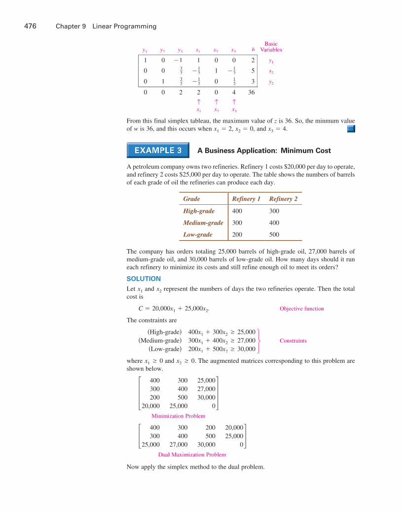
476 Chapter 9 Linear Programming
y1 y2 y3 s1 s2 s3 bBasic
Variables
1 0 −1 1 0 0 2 y1
0 0 32 −1
2 1 −12 5 s2
0 1 32 −1
2 0 12 3 y2
0 0 2 2 0 4 36
→
x1
→
x2
→
x3
From this final simplex tableau, the maximum value of z is 36. So, the minmum value of w is 36, and this occurs when x1 = 2, x2 = 0, and x3 = 4.
a business application: Minimum Cost
A petroleum company owns two refineries. Refinery 1 costs $20,000 per day to operate, and refinery 2 costs $25,000 per day to operate. The table shows the numbers of barrels of each grade of oil the refineries can produce each day.
Grade Refinery 1 Refinery 2
High-grade 400 300
Medium-grade 300 400
Low-grade 200 500
The company has orders totaling 25,000 barrels of high-grade oil, 27,000 barrels of medium-grade oil, and 30,000 barrels of low-grade oil. How many days should it run each refinery to minimize its costs and still refine enough oil to meet its orders?
SoluTion
Let x1 and x2 represent the numbers of days the two refineries operate. Then the total cost is
C = 20,000x1 + 25,000x2. Objective function
The constraints are
(High-grade)(Medium-grade)
(Low-grade)
400x1 + 300x2 ≥ 25,000300x1 + 400x2 ≥ 27,000200x1 + 500x2 ≥ 30,000
Constraints
where x1 ≥ 0 and x2 ≥ 0. The augmented matrices corresponding to this problem are shown below.
[400300200
20,000
300400500
25,000
25,00027,00030,000
0]
Minimization Problem
[400300
25,000
300400
27,000
200500
30,000
20,00025,000
0] Dual Maximization Problem
Now apply the simplex method to the dual problem.
9781305658004_0904.indd 476 12/3/15 2:03 PM

9.4 The Simplex Method: Minimization 477
y1 y2 y3 s1 s2 bBasic
Variables
400 300 200 1 0 20,000 s1
300 400 500 0 1 25,000 s2
−25,000 −27,000 −30,000 0 0 0
→
Entering
y1 y2 y3 s1 s2 bBasic
Variables
280 140 0 1 −25 10,000 s1
35
45 1 0 1
500 50 y3
−7000 −3000 0 0 60 1,500,000
→
Entering
y1 y2 y3 s1 s2 bBasic
Variables
1 12 0 1
280 − 1700
2507 y1
0 12 1 − 3
14001
350200
7 y3
0 500 0 25 50 1,750,000
→
x1
→
x2
From this final simplex tableau, the minimum cost is
C = $1,750,000 Minimum cost
and this occurs when
x1 = 25 and x2 = 50.
So, the two refineries should be operated for the numbers of days shown below.
Refinery 1: 25 days
Refinery 2: 50 days
Note that by operating the two refineries for these numbers of days, the company produces the amounts of oil listed below.
High-grade oil: 400(25) + 300(50) = 25,000 barrelsMedium-grade oil: 300(25) + 400(50) = 27,500 barrelsLow-grade oil: 200(25) + 500(50) = 30,000 barrels
So, the company refines enough of each grade of oil to meet its orders (with a surplus of 500 barrels of medium-grade oil).
linear algebra aPPlieD
Minimization has a wide variety of real-life applications. For example, consider a situation in which steel coils must be custom cut to a precise measurement. This can cause a sizable amount of waste metal. To minimize waste, a manufacturer determines an objective function and establishes detailed constraints on costs, production time, order specifications, and available materials. The manufacturer than uses specialized optimization software to develop a production plan for each order, and can adapt the constraints for different orders, changing conditions, or varying customers’ needs.
Levent Konuk/Shutterstock.com
→ Departing
→ Departing
9781305658004_0904.indd 477 12/3/15 2:03 PM
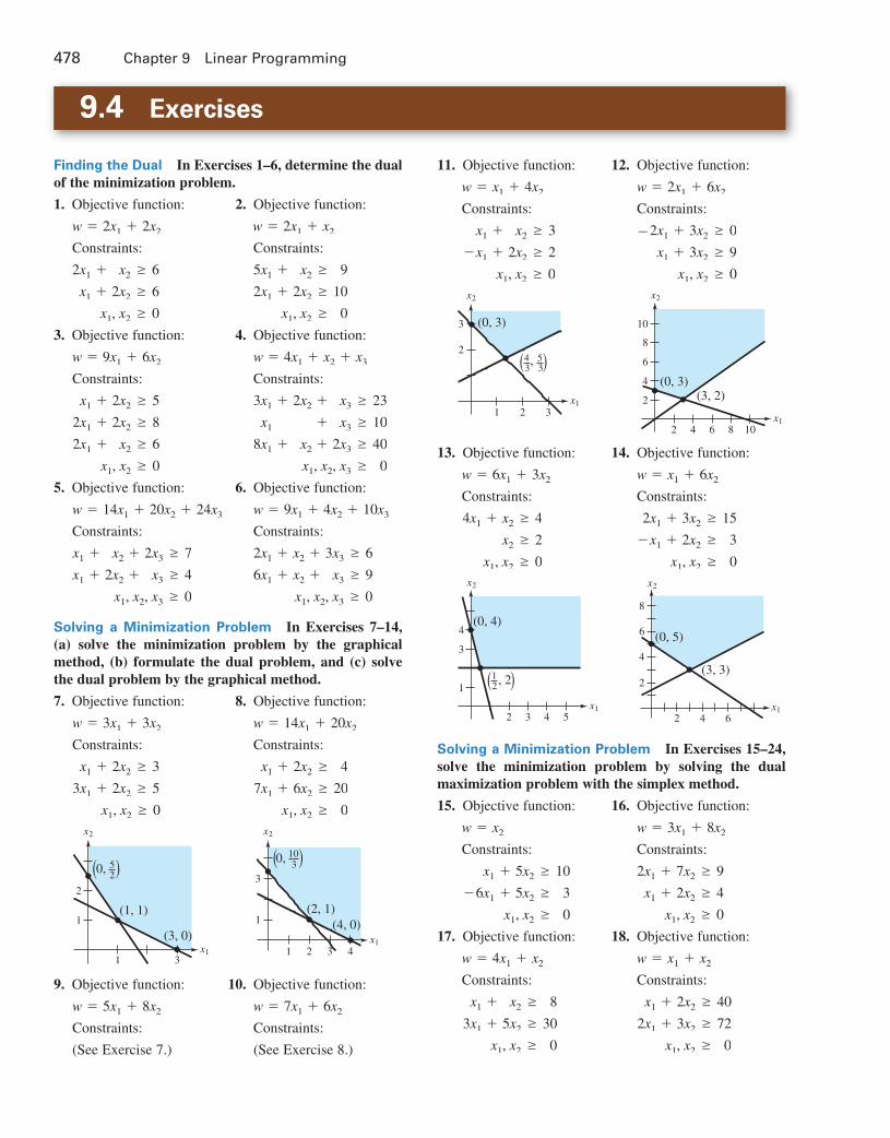
478 Chapter 9 Linear Programming
9.4 Exercises
finding the Dual In Exercises 1–6, determine the dual of the minimization problem.
1. Objective function: 2. Objective function:
w = 2x1 + 2x2 w = 2x1 + x2
Constraints: Constraints:
2x1 +x1 +
x2 ≥ 6
2x2 ≥ 6
5x1 +2x1 +
x2 ≥2x2 ≥
9
10
x1, x2 ≥ 0 x1, x2 ≥ 0
3. Objective function: 4. Objective function:
w = 9x1 + 6x2 w = 4x1 + x2 + x3
Constraints: Constraints:
x1 +2x1 +2x1 +
2x2 ≥ 5
2x2 ≥ 8
x2 ≥ 6
3x1
x1
8x1
+
+
2x2 ++
x2 +
x3 ≥ 23
x3 ≥ 10
2x3 ≥ 40
x1, x2 ≥ 0 x1, x2, x3 ≥ 0
5. Objective function: 6. Objective function:
w = 14x1 + 20x2 + 24x3 w = 9x1 + 4x2 + 10x3
Constraints: Constraints:
x1 +x1 +
x2 +2x2 +
2x3 ≥ 7
x3 ≥ 4
2x1 + x2 +6x1 + x2 +
3x3 ≥ 6
x3 ≥ 9
x1, x2, x3 ≥ 0 x1, x2, x3 ≥ 0
Solving a Minimization Problem In Exercises 7–14, (a) solve the minimization problem by the graphical method, (b) formulate the dual problem, and (c) solve the dual problem by the graphical method.
7. Objective function: 8. Objective function:
w = 3x1 + 3x2 w = 14x1 + 20x2
Constraints: Constraints:
x1 + 2x2 ≥ 3
3x1 + 2x2 ≥ 5
x1 + 2x2 ≥7x1 + 6x2 ≥
4
20
x1, x2 ≥ 0 x1, x2 ≥ 0
x1
x2
1
1
2
3
0, 52
(1, 1)
(3, 0)
( (
x1
x2
0, 103
(2, 1)(4, 0)
1
1
3
2 3 4
( (
9. Objective function: 10. Objective function:
w = 5x1 + 8x2 w = 7x1 + 6x2
Constraints: Constraints:
(See Exercise 7.) (See Exercise 8.)
11. Objective function: 12. Objective function:
w = x1 + 4x2 w = 2x1 + 6x2
Constraints: Constraints:
x1 +
−x1 +x2 ≥ 3
2x2 ≥ 2
−2x1 + 3x2 ≥ 0
x1 + 3x2 ≥ 9
x1, x2 ≥ 0 x1, x2 ≥ 0
x1
x2
4 53 3
(0, 3)
,( (
1 2 3
2
3
(3, 2)(0, 3)
2
2
4
6
8
10
4 6 108x1
x2
13. Objective function: 14. Objective function:
w = 6x1 + 3x2 w = x1 + 6x2
Constraints: Constraints:
4x1 + x2 ≥ 4
x2 ≥ 2
2x1 + 3x2 ≥−x1 + 2x2 ≥
15
3
x1, x2 ≥ 0 x1, x2 ≥ 0
1
3
4
2 43 5x1
x2
(0, 4)
, 212( (
x1
x2
2
2
4
6
8
4 6
(0, 5)
(3, 3)
Solving a Minimization Problem In Exercises 15–24, solve the minimization problem by solving the dual maximization problem with the simplex method.
15. Objective function: 16. Objective function:
w = x2 w = 3x1 + 8x2
Constraints: Constraints:
x1 + 5x2 ≥
−6x1 + 5x2 ≥10
3
2x1 + 7x2 ≥ 9
x1 + 2x2 ≥ 4
x1, x2 ≥ 0 x1, x2 ≥ 0
17. Objective function: 18. Objective function:
w = 4x1 + x2 w = x1 + x2
Constraints: Constraints:
x1 +
3x1 +x2 ≥
5x2 ≥8
30
x1 + 2x2 ≥ 40
2x1 + 3x2 ≥ 72
x1, x2 ≥ 0 x1, x2 ≥ 0
9781305658004_0904.indd 478 12/3/15 2:03 PM

9.4 Exercises 479
19. Objective function: 20. Objective function:
w = x1 + 2x2 w = 2x1 + 5x2
Constraints: Constraints:
3x1 + 5x2 ≥ 15
5x1 + 2x2 ≥ 10
x1 +2x1 +
3x2 ≥x2 ≥
9
12
x1, x2 ≥ 0 x1, x2 ≥ 0
21. Objective function: 22. Objective function:
w = 8x1 + 4x2 + 6x3 w = 8x1 + 16x2 + 18x3
Constraints: Constraints:
3x1 +4x1 +2x1 +
2x2 +x2 +x2 +
x3 ≥ 6
3x3 ≥ 7
4x3 ≥ 8
2x1 +−4x1 +
x1 −
2x2 −3x2 −x2 +
2x3 ≥ 4
x3 ≥ 1
3x3 ≥ 8
x1, x2, x3 ≥ 0 x1, x2, x3 ≥ 0
23. Objective function: 24. Objective function:
w = 6x1 + 2x2 + 3x3 w = 42x1 + 5x2 + 17x3
Constraints: Constraints:
3x1
6x1
3x1
+
+
2x2 ++
x2 +
x3 ≥ 28
x3 ≥ 24
2x3 ≥ 40
3x1 − x2 +−3x1 − x2 +
6x1 + x2 +
7x3 ≥3x3 ≥x3 ≥
5
8
16
x1, x2, x3 ≥ 0 x1, x2, x3 ≥ 0
25. Manufacturing An electronics manufacturing company has three production plants, and each produces three different models of a smart phone. The table shows the daily capacities (in thousands of units) of the three plants.
Basic Model
Gold Model
Platinum Model
Plant 1 8 4 8
Plant 2 6 6 3
Plant 3 12 4 8
The total demands are 300,000 units of the Basic model, 172,000 units of the Gold model, and 249,500 units of the Platinum model. The daily operating costs are $55,000 for plant 1, $60,000 for plant 2, and $60,000 for plant 3. How many days should each plant operate to fill the total demand while keeping the operating cost at a minimum?
26. Manufacturing The company in Exercise 25 lowers the daily operating cost for plant 3 to $50,000. How many days should each plant operate in order to fill the total demand while keeping the operating cost at a minimum?
27. Standard form Use a geometric argument to explain why, for a minimization problem in standard form, the left-hand side of each constraint is greater than or equal to the right-hand side.
28. CAPSTONE Consider the two related optimization problems below.
Problem 1
Objective function:
M = 8y1 + 50y2 + 10y3
Constraints:
2y1 + y2
y1 + y2
+ 2y3 ≤≤
y3 ≥
5
10
6y1 − 65
y1, y2, y3 ≥ 0
Problem 2
Objective function:
N = 5x1 + 10x2 + 65x3
Constraints:
2x1 + x2
x1 + x2
+ 6x3 ≥≥
x3 ≤
8
50
2x1 − 10
x1, x2, x3 ≥ 0
(a) Which is the minimization problem? Explain.
(b) Which is the dual maximization problem? Explain.
(c) Write the corresponding augmented matrices and explain how they are related.
optimal Cost In Exercises 29–32, two sports drinks supply protein and carbohydrates. Drink A provides 1 unit of protein and 3 units of carbohydrates in each liter. Drink B supplies 2 units of protein and 2 units of carbohydrates in each liter. An athlete requires 3 units of protein and 5 units of carbohydrates. Find the amount of each drink the athlete should consume to minimize the cost and still meet the minimum dietary requirements.
29. Drink A costs $2 per liter and drink B costs $3 per liter.
30. Drink A costs $4 per liter and drink B costs $2 per liter.
31. Drink A costs $1 per liter and drink B costs $3 per liter.
32. Drink A costs $1 per liter and drink B costs $2 per liter.
Minimizing a function In Exercises 33 and 34, use a software program or a graphing utility to minimize the objective function subject to the constraints
1.5x1
x1
0.5x1
+
+
x2
2x2
x2
+++
+6x3 +x3 +
2.5x3 +
2x4 ≥4x4 ≥x4 ≥
1.5x4 ≥
35
120
50
75
where x1, x2, x3, x4 ≥ 0.
33. w = x1 + 0.5x2 + 2.5x3 + 3x4
34. w = 1.5x1 + x2 + 0.5x3 + 2x4
9781305658004_0904.indd 479 12/3/15 2:03 PM

480 Chapter 9 Linear Programming
9.5 The Simplex Method: Mixed Constraints
Find the maximum of an objective function subject to mixed constraints.
Find the minimum of an objective function subject to mixed constraints.
Mixed Constraints and MaxiMization
In Sections 9.3 and 9.4, you studied linear programming problems in standard form. The constraints for the maximization problems all involved ≤ inequalities, and the constraints for the minimization problems all involved ≥ inequalities.
As mentioned earlier, linear programming problems for which the constraints involve both types of inequalities are called mixed-constraint problems. For example, consider the linear programming problem below.
Mixed-Constraint Problem: Find the maximum value of
z = x1 + x2 + 2x3 Objective function
subject to the constraints
2x1
2x1
x1
+ x2
+ x2
+ x3 ≤ 50≥ 36
+ x3 ≥ 10 Constraints
where x1 ≥ 0, x2 ≥ 0, and x3 ≥ 0. This is a maximization problem, so you would expect each of the inequalities in the set of constraints to involve ≤. The first inequality does involve ≤, so add a slack variable to form the equation
2x1 + x2 + x3 + s1 = 50.
For the other two inequalities, a new type of variable, a surplus variable, is introduced, as shown below.
2x1
x1
+ x2
+ x3
− s2 = 36− s3 = 10
Notice that surplus variables are subtracted from (not added to) the left side of each equation. They are called surplus variables because they represent the amounts by which the left sides of the inequalities exceed the right sides. Surplus variables must be nonnegative.
Now, to solve the problem, form an initial simplex tableau, as shown below.
x1 x2 x3 s1 s2 s3 bBasic
Variables
2 1 1 1 0 0 50 s1
2 1 0 0 −1 0 36 s2
1 0 1 0 0 −1 10 s3
−1 −1 −2 0 0 0 0
Solving mixed-constraint problems can be difficult. One reason for this is that there is no convenient feasible solution to begin the simplex method. Note that the solution represented by the initial tableau above
(x1, x2, x3, s1, s2, s3) = (0, 0, 0, 50, −36, −10)
is not a feasible solution because the values of the two surplus variables are negative.
reMarKIn fact, the values x1 = x2 = x3 = 0 do not even satisfy the constraint equations.
9781305658004_0905.indd 480 12/3/15 2:05 PM

9.5 The Simplex Method: Mixed Constraints 481
To eliminate the surplus variables from the current solution, use “trial and error.” That is, in an effort to find a feasible solution, arbitrarily choose new entering variables. For example, it seems reasonable to select x3 as the entering variable, because its column has the most negative entry in the bottom row.
x1 x2 x3 s1 s2 s3 bBasic
Variables
2 1 1 1 0 0 50 s1
2 1 0 0 −1 0 36 s2
1 0 1 0 0 −1 10 s3
−1 −1 −2 0 0 0 0
→
Entering
After pivoting, the new simplex tableau is as shown below.
x1 x2 x3 s1 s2 s3 bBasic
Variables
1 1 0 1 0 1 40 s1
2 1 0 0 −1 0 36 s2
1 0 1 0 0 −1 10 x3
1 −1 0 0 0 −2 20
→
Entering
The current solution (x1, x2, x3, s1, s2, s3) = (0, 0, 10, 40, −36, 0) is still not feasible, so choose x2 as the entering variable and pivot to obtain the simplex tableau below.
x1 x2 x3 s1 s2 s3 bBasic
Variables
−1 0 0 1 1 1 4 s1
2 1 0 0 −1 0 36 x2
1 0 1 0 0 −1 10 x3
3 0 0 0 −1 −2 56
→
Entering
At this point, you obtain a feasible solution
(x1, x2, x3, s1, s2, s3) = (0, 36, 10, 4, 0, 0).
From here, continue by applying the simplex method as usual. Note that the next entering variable is s3. After pivoting one more time, you obtain the final simplex tableau shown below.
x1 x2 x3 s1 s2 s3 bBasic
Variables
−1 0 0 1 1 1 4 s3
2 1 0 0 −1 0 36 x2
0 0 1 1 1 0 14 x3
1 0 0 2 1 0 64
Note that this tableau is final because it represents a feasible solution and there are no negative entries in the bottom row. So, the maximum value of the objective function is z = 64 and this occurs when x1 = 0, x2 = 36, and x3 = 14.
→ Departing
→ Departing
→ Departing
9781305658004_0905.indd 481 12/3/15 2:05 PM

482 Chapter 9 Linear Programming
a Maximization Problem with Mixed Constraints
Find the maximum value of
z = 3x1 + 2x2 + 4x3 Objective function
subject to the constraints
3x1 +4x1 +2x1 +
2x2 +2x2 +x2 +
5x3 ≤3x3 ≤x3 ≥
18164 Constraints
where x1 ≥ 0, x2 ≥ 0, and x3 ≥ 0.
solution
To begin, add a slack variable to each of the first two inequalities and subtract a surplus variable from the third inequality to produce the system of linear equations below.
3x1 +4x1 +2x1 +
2x2 +2x2 +x2 +
5x3
3x3
x3
+ s1
+ s2
==
− s3 =
18164
Next form the initial simplex tableau.
x1 x2 x3 s1 s2 s3 bBasic
Variables
3 2 5 1 0 0 18 s1
4 2 3 0 1 0 16 s2
2 1 1 0 0 −1 4 s3
−3 −2 −4 0 0 0 0
This tableau does not represent a feasible solution because the value of s3 is negative. So, s3 should be the departing variable. There are no real guidelines as to which variable should enter the solution, and in fact, any choice will work. However, some entering variables will require more tedious computations than others. For example, choosing x1 as the entering variable produces the tableau below.
x1 x2 x3 s1 s2 s3 bBasic
Variables
0 12
72 1 0 3
2 12 s1
0 0 1 0 1 2 8 s2
1 12
12 0 0 −1
2 2 x1
0 −12 −5
2 0 0 −32 6
Choosing x2 as the entering variable on the initial tableau instead produces the tableau shown below, which contains “nicer” numbers.
x1 x2 x3 s1 s2 s3 bBasic
Variables
−1 0 3 1 0 2 10 s1
0 0 1 0 1 2 8 s2
2 1 1 0 0 −1 4 x2
1 0 −2 0 0 −2 8
Choosing x3 as the entering variable on the initial tableau will also produce a tableau that does not contain fractions. (Verify this.)
→ Departing
9781305658004_0905.indd 482 12/3/15 2:05 PM

9.5 The Simplex Method: Mixed Constraints 483
Notice that both of the tableaus shown represent feasible solutions. Any choice of entering variables will lead to a feasible solution, so use trial and error to find an entering variable that yields “nice” numbers. Once you have reached a feasible solution, follow the standard pivoting procedure to choose entering variables and eventually reach an optimal solution.
The rest of this solution uses the tableau produced by choosing x2 as the entering variable. This tableau does represent a feasible solution, so proceed as usual, choosing the most negative entry in the bottom row to be the entering variable. (In this case, there is a tie, so arbitrarily choose x3 to be the entering variable.)
x1 x2 x3 s1 s2 s3 bBasic
Variables
−1 0 3 1 0 2 10 s1
0 0 1 0 1 2 8 s2
2 1 1 0 0 −1 4 x2
1 0 −2 0 0 −2 8
→
Entering
x1 x2 x3 s1 s2 s3 bBasic
Variables
−13 0 1 1
3 0 23
103 x3
13 0 0 −1
3 1 43
143 s2
73 1 0 −1
3 0 −53
23 x2
13 0 0 2
3 0 −23
443
→Entering
x1 x2 x3 s1 s2 s3 bBasic
Variables
−12 0 1 1
2 −12 0 1 x3
14 0 0 −1
434 1 7
2 s3
114 1 0 −3
454 0 13
2 x2
12 0 0 1
212 0 17
So, the maximum value of the objective function is z = 17, and this occurs when
x1 = 0, x2 = 132 , and x3 = 1.
reMarKVerify that choosing x1 or x3 as the entering variable on the initial simplex tableau yields the same solution.
linear algebra aPPlied
As with standard form maximization and minimization, mixed constraint optimization has a wide variety of real-life applications. For example, in Exercise 55 you are asked to determine how to allocate a company’s advertising budget to maximize the total audience. This type of mixed constraint problem is typical in advertising because market research establishes minimums on the number of each type of ad, while budgets put upper limits on expenses. To maximize an audience, researchers must first determine the ideal demographic and then estimate the time and place at which those people will most likely see the ad, considering traditional venues as well as digital formats and social media. Other common real-life applications of constrained optimization problems involve minimizing costs.
→ Departing
→ Departing
LIDOphotography/Shutterstock.com
9781305658004_0905.indd 483 12/3/15 2:05 PM

484 Chapter 9 Linear Programming
Mixed Constraints and MiniMization
Section 9.4 discusses the solution of minimization problems in standard form. Minimization problems that are not in standard form are more difficult to solve. One technique is to change a mixed-constraint minimization problem to a mixed-constraint maximization problem by multiplying each coefficient in the objective function by −1. The next example demonstrates this technique.
a Minimization Problem with Mixed Constraints
See LarsonLinearAlgebra.com for an interactive version of this type of example.
Find the minimum value of
w = 4x1 + 2x2 + x3 Objective function
subject to the constraints
2x1 +3x1 +x1 +
3x2 +x2 +
4x2 +
4x3 ≤5x3 ≥3x3 ≥
1446 Constraints
where x1 ≥ 0, x2 ≥ 0, and x3 ≥ 0.
solution
First, rewrite the objective function by multiplying each of its coefficients by −1, as shown below.
z = −4x1 − 2x2 − x3 Revised objective function
Maximizing this revised objective function is equivalent to minimizing the original objective function. Next, add a slack variable to the first inequality and subtract surplus variables from the second and third inequalities to produce the initial simplex tableau below.
x1 x2 x3 s1 s2 s3 bBasic
Variables
2 3 4 1 0 0 14 s1
3 1 5 0 −1 0 4 s2
1 4 3 0 0 −1 6 s3
4 2 1 0 0 0 0
Note that the bottom row contains the negatives of the coefficients of the revised objective function. Another way of looking at this is that when using this technique to solve minimization problems in nonstandard form, the bottom row of the initial simplex tableau consists of the coefficients of the original objective function.
As with maximization problems with mixed constraints, this initial simplex tableau does not represent a feasible solution. By trial and error, choose x2 as the entering variable and s2 as the departing variable.
x1 x2 x3 s1 s2 s3 bBasic
Variables
2 3 4 1 0 0 14 s1
3 1 5 0 −1 0 4 s2
1 4 3 0 0 −1 6 s3
4 2 1 0 0 0 0
→
Entering
→ Departing
9781305658004_0905.indd 484 12/3/15 2:05 PM

9.5 The Simplex Method: Mixed Constraints 485
After pivoting, you obtain the tableau shown below.
x1 x2 x3 s1 s2 s3 bBasic
Variables
−7 0 −11 1 3 0 2 s1
3 1 5 0 −1 0 4 x2
−11 0 −17 0 4 −1 −10 s3
−2 0 −9 0 2 0 −8
To transform the tableau into one that represents a feasible solution, multiply the third row by −1.
x1 x2 x3 s1 s2 s3 bBasic
Variables
−7 0 −11 1 3 0 2 s1
3 1 5 0 −1 0 4 x2
11 0 17 0 −4 1 10 s3
−2 0 −9 0 2 0 −8
Now that you have obtained a simplex tableau that represents a feasible solution, continue with pivoting operations until you obtain an optimal solution.
x1 x2 x3 s1 s2 s3 bBasic
Variables
−7 0 −11 1 3 0 2 s1
3 1 5 0 −1 0 4 x2
11 0 17 0 −4 1 10 s3
−2 0 −9 0 2 0 −8
→
Entering
x1 x2 x3 s1 s2 s3 bBasic
Variables2
17 0 0 1 717
1117
14417 s1
− 417 1 0 0 3
17 − 517
1817 x2
1117 0 1 0 − 4
171
171017 x3
6517 0 0 0 − 2
179
17 −4617
→
Entering
x1 x2 x3 s1 s2 s3 bBasic
Variables23 −7
3 0 1 0 43 6 s1
−43
173 0 0 1 −5
3 6 s2
13
43 1 0 0 −1
3 2 x3
113
23 0 0 0 1
3 −2
The maximum value of the revised objective function is z = −2, and so the minimum value of the original objective function is
w = 2
(the negative of the entry in the lower-right corner). This occurs when
x1 = 0, x2 = 0, and x3 = 2.
reMarKRecall from page 458 that your choices for the entering variable exclude the entry in the “b-column.” So, although −46
17 is the least entry in the bottom row here, it does not represent a variable that can enter the solution.
→ Departing
→ Departing
9781305658004_0905.indd 485 12/3/15 2:05 PM

486 Chapter 9 Linear Programming
a business application: Minimum shipment Costs
An automobile company has two factories. One factory has 400 cars of one model in stock and the other factory has 300 cars (of the same model) in stock. Two customers order this car model. The first customer needs 200 cars, and the second customer needs 300 cars. The table shows the costs of shipping cars from the two factories to the customers.
Customer 1 Customer 2
Factory 1 $30 $25
Factory 2 $36 $30
How should the company ship the cars to minimize the shipping costs? What is the minimum cost?
solution
To begin, let x1 and x2 represent the numbers of cars shipped from factory 1 to the first and second customers, respectively. This means that the number of cars shipped from factory 2 to the first customer is
200 − x1
and that the number of cars shipped from factory 2 to the second customer is
300 − x2.
(See figure.)
Customer 1 Customer 2
$30 $25
$36 $30
x1
200 − x1
x2
300 − x2
Factory 1
Factory 2
The total cost of shipping is
C = 30x1 + 25x2 + 36(200 − x1) + 30(300 − x2) = 16,200 − 6x1 − 5x2.
The constraints for this minimization problem are as listed below.
x1 + x2 ≤ 400
(200 − x1) + (300 − x2) ≤ 300
x1 ≤ 200
x2 ≤ 300
x1 + x2 ≥ 200
The corresponding maximization problem is to maximize z = 6x1 + 5x2 − 16,200. The initial simplex tableau is shown below.
x1 x2 s1 s2 s3 s4 bBasic
Variables
1 1 1 0 0 0 400 s1
1 1 0 −1 0 0 200 s2
1 0 0 0 1 0 200 s3
0 1 0 0 0 1 300 s4
−6 −5 0 0 0 0 −16,200
9781305658004_0905.indd 486 12/3/15 2:05 PM

9.5 The Simplex Method: Mixed Constraints 487
Note that the current z-value is −16,200 because
z = 6x1 + 5x2 − 16,200 = 6(0) + 5(0) − 16,200 = −16,200.
Now, to the initial tableau, apply the simplex method, as shown below.
x1 x2 s1 s2 s3 s4 bBasic
Variables
1 1 1 0 0 0 400 s1
1 1 0 −1 0 0 200 s2
1 0 0 0 1 0 200 s3
0 1 0 0 0 1 300 s4
−6 −5 0 0 0 0 −16,200
→
Entering
x1 x2 s1 s2 s3 s4 bBasic
Variables
0 0 1 1 0 0 200 s1
1 1 0 −1 0 0 200 x1
0 −1 0 1 1 0 0 s3
0 1 0 0 0 1 300 s4
0 1 0 −6 0 0 −15,000
→
Entering
x1 x2 s1 s2 s3 s4 bBasic
Variables
0 1 1 0 −1 0 200 s1
1 1 0 0 1 0 200 x1
0 −1 0 1 1 0 0 s2
0 1 0 0 0 1 300 s4
0 −5 0 0 6 0 −15,000
→
Entering
x1 x2 s1 s2 s3 s4 bBasic
Variables
0 1 1 0 −1 0 200 x2
1 0 0 0 1 0 200 x1
0 0 1 1 0 0 200 s2
0 0 −1 0 1 1 100 s4
0 0 5 0 1 0 −14,000
From this final simplex tableau, the minimum shipping cost is $14,000. x1 = 200 and x2 = 200, so you can conclude that the numbers of cars that should ship from the two factories are as shown in the table.
Customer 1 Customer 2
Factory 1 200 cars 200 cars
Factory 2 0 100 cars
→ Departing
→ Departing
→ Departing
9781305658004_0905.indd 487 12/3/15 2:05 PM

488 Chapter 9 Linear Programming
9.5 Exercises
slack and surplus Variables In Exercises 1–8, add the appropriate slack and surplus variables to the system and form the initial simplex tableau.
1. (Maximize) 2. (Maximize) Objective function: Objective function:
z = 10x1 + 4x2 z = x1 + 5x2
Constraints: Constraints:
2x1 + x2 ≥ 4
x1 + x2 ≤ 8
x1 +3x1 +
x2 ≤ 16
2x2 ≥ 19
x1, x2 ≥ 0 x1, x2 ≥ 0
3. (Minimize) 4. (Minimize) Objective function: Objective function:
w = x1 + x2 w = 2x1 + 3x2
Constraints: Constraints:
2x1 +x1 +
x2 ≤ 4
3x2 ≥ 2
3x1 +4x1 +
x2 ≥ 4
2x2 ≤ 3
x1, x2 ≥ 0 x1, x2 ≥ 0
5. (Maximize) 6. (Minimize) Objective function: Objective function:
z = x1 + x3 w = 3x1 + x2 + x3
Constraints: Constraints:
4x1 + x2
x1 + x2
2x1 + x2
≥ 10
+ 3x3 ≤ 30
+ 4x3 ≥ 16
x1 +
4x1 −
2x2 +x2 +x2 +
x3 ≤5x3 ≥x3 ≥
10
6
16
x1, x2, x3 ≥ 0 x1, x2, x3 ≥ 0
7. (Minimize) 8. (Maximize) Objective function: Objective function:
w = 4x1 + 2x2 + x3 z = 4x1 + x2 + x3
Constraints: Constraints:
5x1 + 4x2
x1 + 6x2
+ 5x3 ≥≤
12
5
2x1 + x2 +x2 +
4x3 ≤ 60
x3 ≥ 40
x1, x2, x3 ≥ 0 x1, x2, x3 ≥ 0
solving a Mixed-Constraint Problem In Exercises 9–14, use the specified entering and departing variables to solve the mixed-constraint problem.
9. (Maximize) 10. (Maximize) Objective function: Objective function:
z = −x1 + 2x2 z = 2x1 + x2
Constraints: Constraints:
x1 + x2 ≥ 3
x1 + x2 ≤ 6
x1 + x2 ≥ 4
x1 + x2 ≤ 8
x1, x2 ≥ 0 x1, x2 ≥ 0
Entering x2, departing s1 Entering x1, departing s1
11. (Minimize) 12. (Minimize) Objective function: Objective function:
w = x1 + 2x2 w = 3x1 + 2x2
Constraints: Constraints:
2x1 + 3x2 ≤ 25
x1 + 2x2 ≥ 16
x1 +3x1 +
x2 ≥ 20
4x2 ≤ 70
x1, x2 ≥ 0 x1, x2 ≥ 0
Entering x2, departing s2 Entering x1, departing s1
13. (Maximize) 14. (Maximize) Objective function: Objective function:
z = x1 + x2 z = x1 + 2x2 + 2x3
Constraints: Constraints:
−4x1 +−2x1 +
3x2 + x3 ≤ 40
x2 + x3 ≥ 10
x2 + x3 ≤ 20
x1 + x2
2x1 + x2
x2
++
≥ 50
x3 ≤ 70
3x3 ≥ 40
x1, x2, x3 ≥ 0 x1, x2, x3 ≥ 0
Entering x2, departing s2 Entering x2, departing s1
solving a Mixed-Constraint Problem In Exercises 15–20, rework the stated exercise using the specified entering and departing variables.
15. Exercise 9; entering x1, departing s1
16. Exercise 10; entering x2, departing s1
17. Exercise 11; entering x1, departing s2
18. Exercise 12; entering x2, departing s1
19. Exercise 13; entering x1, departing s2
20. Exercise 14; entering x1, departing s1
solving a Mixed-Constraint Problem In Exercises 21–30, use the simplex method to solve the problem.
21. (Maximize) 22. (Maximize) Objective function: Objective function:
z = 2x1 + 5x2 z = −x1 + 3x2
Constraints: Constraints:
x1 +x1 +
2x2 ≥ 4
x2 ≤ 8
2x1 +x1 +
x2 ≤ 4
5x2 ≥ 5
x1, x2 ≥ 0 x1, x2 ≥ 0
23. (Maximize) 24. (Minimize) Objective function: Objective function:
z = x1 + 3x2 w = 5x1 + 3x2
Constraints: Constraints:
2x1 + x2 ≤ 36
x1 + x2 ≥ 18
3x1 −x1 +
4x2 ≥ 2812x2 ≤ 64
x1, x2 ≥ 0 x1, x2 ≥ 0
9781305658004_0905.indd 488 12/3/15 2:05 PM

9.5 Exercises 489
25. (Minimize) 26. (Minimize) Objective function: Objective function:
w = x1 + x2 w = 2x1 + 3x2
Constraints: Constraints:
x1 + 2x2 ≥ 25
2x1 + 5x2 ≤ 60
3x1 +x1 +
2x2 ≤ 22
x2 ≥ 10
x1, x2 ≥ 0 x1, x2 ≥ 0
27. (Maximize) 28. (Maximize) Objective function: Objective function:
z = 2x1 + x2 + 3x3 z = 3x1 + 5x2 + 2x3
Constraints: Constraints:
x1 +
3x1 +
4x2
x2
2x2
+−+
2x3 ≤ 85
5x3 ≥ 20
11x3 ≥ 49
9x1 +5x1 +4x1 +
4x2
2x2
x2
+ x3 ≥ 70
+ x3 ≤ 40
≥ 16
x1, x2, x3 ≥ 0 x1, x2, x3 ≥ 0
29. (Minimize) 30. (Minimize) Objective function: Objective function:
w = −2x1 + 4x2 − x3 w = x1 + x2 + x3
Constraints: Constraints:
3x1 − 6x2 +2x1 − 8x2 +
4x3 ≤ 30
10x3 ≥ 18
x1 +
x1 +
2x2 +6x2 +x2 +
x3 ≥ 30
x3 ≤ 54
3x3 ≥ 20
x1, x2, x3 ≥ 0
x1, x2, x3 ≥ 0
Maximizing with Mixed Constraints In Exercises 31–38, maximize the objective function subject to the constraints listed below.
x1 + x2 ≤ 5−x1 + x2 ≤ 3
x2 ≥ 1x1, x2 ≥ 0
31. z = 2x1 + x2 32. z = x1 + 2x2
33. z = x2 34. z = −x1 − x2
35. z = −3x1 + 2x2 36. z = 3x1
37. z = 4x1 + 5x2 38. z = −4x1 + 2x2
Maximizing with Mixed Constraints In Exercises 39–46, maximize the objective function subject to the constraints listed below.
3x1
x1
−x1
x1
+−+
2x2 ≥ 6x2 ≤ 2
2x2 ≤ 6≤ 4
x1, x2 ≥ 0
39. z = −3x2 40. z = 4x1
41. z = x1 + x2 42. z = x1 − 2x2
43. z = −4x1 + x2 44. z = 4x1 − x2
45. z = −2x1 − 2x2 46. z = −6x1 + 2x2
Minimizing Cost In Exercises 47–50, a tire company has two suppliers, S1 and S2, S1 has 900 tires on hand and S2 has 800 tires on hand. Customer C1 needs 500 tires and customer C2 needs 600 tires. Minimize the cost of filling the orders subject to the data in the table (shipping costs per tire).
47. C1 C2
S1 0.60 1.20
S2 1.00 1.80
48. C1 C2
S1 0.80 1.00
S2 1.00 1.20
49. C1 C2
S1 1.20 1.00
S2 1.00 1.20
50. C1 C2
S1 0.80 1.00
S2 1.00 0.80
Minimizing Cost In Exercises 51 and 52, a manufacturer has two assembly plants, plant A and plant B, and two distribution outlets, outlet I and outlet II. Plant A can assemble 5000 units of a product in a year and plant B can assemble 4000 units of the same product in a year. Outlet I must have 3000 units per year and outlet II must have 5000 units per year. The table shows the costs of transportation from each plant to each outlet. Find the shipping schedule that will produce the minimum cost. What is the minimum cost?
51. Outlet I Outlet II
Plant A $4 $5
Plant B $5 $6
52. Outlet I Outlet II
Plant A $4 $5
Plant B $6 $4
53. Minimizing Cost An automobile company has two factories. One factory has 400 cars of one model in stock and the other factory has 300 cars (of the same model) in stock. Two customers order this car model. The first customer needs 200 cars, and the second customer needs 300 cars. The table shows the costs of shipping cars from the two factories to the two customers.
Customer 1 Customer 2
Factory 1 $36 $30
Factory 2 $30 $25
(a) How should the company ship the cars to minimize the shipping costs?
(b) What is the minimum cost?
9781305658004_0905.indd 489 12/3/15 2:05 PM

490 Chapter 9 Linear Programming
54. Minimizing Cost Rework Exercise 53 assuming that the shipping costs for the two factories are as shown in the table below.
Customer 1 Customer 2
Factory 1 $25 $30
Factory 2 $35 $30
55. advertising A company is determining how to advertise a product nationally on television and in a newspaper. Each television ad is expected to be seen by 15 million viewers, and each newspaper ad is expected to be seen by 3 million readers. The company has the constraints below.
(a) The company has budgeted a maximum of $600,000 to advertise the product.
(b) Each minute of television time costs $60,000 and each one-page newspaper ad costs $15,000.
(c) The company’s market research department recommends using at least 6 television ads and at least 4 newspaper ads.
How should the company allocate its advertising budget to maximize the total audience? What is the maximum audience?
56. CAPSTONE Consider the initial simplex tableau below.
x1 x2 x3 s1 s2 s3 bBasic
Variables
3 −1 8 a 0 0 48 s1
0 12 4 0 b 0 96 s2
−2 2 0 0 0 c 5 s3
−9 −5 −2 0 0 0 0
(a) Does this tableau represent a maximization problem or a minimization problem? Explain.
(b) Find values of a, b, and c such that the solution is feasible.
(c) Use your answer to part (b) to write an objective function and a set of constraints that the simplex tableau could be used to represent.
(d) Find values of a, b, and c such that the solution is not feasible.
(e) Let a = 1, b = 1, and c = 1. Which variable should you choose as the departing variable in the first iteration of pivoting? Explain.
(f) Say you perform the simplex method on the tableau above and obtain a final simplex tableau. Does the entry in the lower-right corner represent the optimal value of the original objective function, or its opposite? Explain.
identifying Feasible solutions In Exercises 57–62, determine whether the simplex tableau represents a feasible solution. Explain.57.
x1 x2 s1 s2 bBasic
Variables
25 −19 1 0 12 s1
−19 25 0 1 12 s2
6 −6 0 0 0
58. x1 x2 s1 s2 b
BasicVariables
5 15 −1 0 60 s1
2 −2 0 1 8 s2
25 20 0 0 0
59. x1 x2 s1 s2 b
BasicVariables
3 9 −1 0 −28 s1
8 4 0 −1 −36 s2
−16 72 0 0 0
60. x1 x2 s1 s2 s3 b
BasicVariables
−14 13 1 0 0 4 s1
−10 2 0 −1 0 3 s2
−8 6 0 0 1 5 s3
−2 −2 0 0 0 0
61. x1 x2 s1 s2 s3 b
BasicVariables
1 2 1 0 0 32 s1
1 −5 0 1 0 10 s2
0 2 0 0 −1 −50 s3
−4 −8 0 0 0 0
62. x1 x2 x3 s1 s2 s3 b
BasicVariables
−10 0 1 −1 0 0 75 s1
0 0 5 0 −1 0 30 s2
3 1 12 0 0 1 26 s3
7 −24 16 0 0 0 0
true or False? In Exercises 63 and 64, determine whether each statement is true or false. If a statement is true, give a reason or cite an appropriate statement from the text. If a statement is false, provide an example that shows the statement is not true in all cases or cite an appropriate statement from the text.
63. One technique that can be used to change a mixed-constraint minimization problem to a mixed-constraint maximization problem is to multiply each coefficient of the objective function by −1.
64. Surplus variables, like slack variables, are always positive because they represent the amount by which the left side of the inequality is less than the right side.
9781305658004_0905.indd 490 12/3/15 2:05 PM

Review Exercises 491
9 Review Exercises
Solving a System of Inequalities In Exercises 1–6, sketch the graph (and label any vertices) of the solution set of the system of inequalities.
1. x +3x +
2y ≤y ≤x ≥y ≥
160180
00
2. 2x +2x +
3y ≤y ≤x ≥y ≥
241600
3. 3x +x +2 ≤
2y ≥ 242y ≥ 12x ≤ 15y ≤ 15
4. 2x +x +0 ≤0 ≤
y ≥ 163y ≥ 18x ≤ 25y ≤ 15
5. 2x −2x −0 ≤
3y ≥ 0y ≤ 8y < 1
6. x −
2x +y ≤
3y <x ≥
10300
Solving a Linear Programming Problem In Exercises 7–18, find the minimum and maximum values of the objective function (if possible), and where they occur, by the graphical method.
7. Objective function: 8. Objective function:
z = 3x + 4y z = 10x + 7y
Constraints: Constraints:
2x +4x +
x ≥y ≥
5y ≤y ≤
00
5028
2x +x +
x ≥y ≥y ≥y ≥
00
10075
x
y
2 4 6 8 10−2
2
4
6
8
10(0, 10)
(5, 8)
(0, 0) (7, 0)
25 50 75 100−25
25
50
75
100
x
y
(0, 100)
(25, 50)
(75, 0)
9. Objective function: 10. Objective function:
z = 4x + 3y z = 2x + 8y
Constraints: Constraints:
x ≥ 0y ≥ 0
x + y ≤ 5
x ≥ 0y ≥ 0
2x − y ≤ 4
1 2 3 4 5 6
123456
(0, 5)
(5, 0)(0, 0)x
y
(0, 0) (2, 0)
(0, 4)
−1 1 2 3
2
3
4
y
x
11. Objective function: 12. Objective function:
z = 25x + 30y z = 15x + 20y
Constraints: Constraints:
0 ≤0 ≤
5x +
x ≤y ≤
6y ≤
6045
420
x ≥y ≥
8x + 9y ≤8x + 9y ≥
00
72003600
(0, 45)(30, 45)
(60, 20)
(60, 0)(0, 0)
20 40 60
20
40
60
x
y
400
400
800 (0, 800)(0, 400)
(900, 0)
(450, 0)x
y
13. Objective function: 14. Objective function:
z = 5x + 0.5y z = 2x + y
Constraints: Constraints:
−x +3x +
x ≥y ≥
3y ≤y ≤
00
7575
2x +3x −x +
x ≥3y ≥y ≤
4y ≤
069
16
(25, 0)(0, 0)
(0, 25)
(15, 30)
x
y
5 10 15 20 25 30
5
10
15
20
25
30
(4, 3)(0, 4)
1 2 4 53
2
1
3
4
5
(0, 2)
(3, 0)x
y
15. Objective function: 16. Objective function:
z = x + 3y z = 4x − y
Constraints: Constraints:
x +x −x +
x ≥y ≥y ≥y ≤
5y ≤
0033
15
x +
3x −
x ≥y ≥y ≥x ≥y ≤
002y
12
17. Objective function: 18. Objective function:
z = 3x − y z = x − 2y
Constraints: Constraints:
x ≥y ≥x ≤
−x + 2y ≤4x + 3y ≤
00
3y1240
5x +5x −2x +
x ≥y ≥y ≤
2y ≥5y ≥
00
364
19
9781305658004_090R.indd 491 12/3/15 2:06 PM

492 Chapter 9 Linear Programming
Using the Simplex Method In Exercises 19–26, use the simplex method to maximize the objective function, subject to the constraints.
19. Objective function: 20. Objective function:
z = x1 + 2x2 z = 5x1 + 4x2
Constraints: Constraints:
2x1 +x1 +
x2 ≤ 314x2 ≤ 40
x1 −x1 +
x2 ≤ 222x2 ≤ 43
x1, x2 ≥ 0 x1, x2 ≥ 0
21. Objective function: 22. Objective function:
z = x1 + 2x2 + x3 z = 4x1 + 5x2 + 6x3
Constraints: Constraints:
2x1 +x1 +
−2x1 +
2x2 +x2 −x2 −
x3 ≤2x3 ≤2x3 ≤
20238
4x1 +x1 +x1 +
2x2 +3x2 +x2 +
x3 ≤ 302x3 ≤ 542x3 ≤ 24
x1, x2, x3 ≥ 0 x1, x2, x3 ≥ 0
23. Objective function: 24. Objective function:
z = x1 + x2 z = 6x1 + 8x2
Constraints: Constraints:
3x1 +x1 +
x2 ≤ 4324x2 ≤ 628
20x1 + 40x2 ≤ 20030x1 + 42x2 ≤ 228
x1, x2 ≥ 0 x1, x2 ≥ 0
25. Objective function: 26. Objective function:
z = 3x1 + 5x2 + 4x3 z = 2x1 + 5x2 − x3
Constraints: Constraints:
6x1 −3x1 −
−2x1 +
2x2 + 3x3 ≤ 243x2 + 9x3 ≤ 33x2 − 2x3 ≤ 25
−x1 +
−2x1 +3x1 +
3x2 +2x2 +x2 −
2x3 ≤ 9212x3 ≤ 766x3 ≤ 24
x1, x2, x3 ≥ 0 x1, x2, x3 ≥ 0
Finding the Dual In Exercises 27 and 28, determine the dual of the minimization problem.
27. Objective function: 28. Objective function:
w = 7x1 + 3x2 + x3 w = 2x1 + 3x2 + 4x3
Constraints: Constraints:
x1 +
3x1 +x2 +
6x2 +2x3 ≥ 304x3 ≥ 75
x1 + 5x2 +x1 + 2x2 +
3x1 + 2x2 +
3x3 ≥ 90x3 ≥ 75x3 ≥ 56
x1, x2, x3 ≥ 0
x1, x2, x3 ≥ 0
Solving a Minimization Problem In Exercises 29–34, solve the minimization problem by solving the dual maximization problem by the simplex method.
29. Objective function: 30. Objective function:
w = 9x1 + 15x2 w = 16x1 + 18x2
Constraints: Constraints:
x1 +
4x1 −5x2 ≥
10x2 ≥150
2x1 − 3x2 ≥−4x1 + 9x2 ≥
148
x1, x2 ≥ 0 x1, x2 ≥ 0
31. Objective function: 32. Objective function:
w = 24x1 + 22x2 + 18x3 w = 32x1 + 36x2 + 4x3
Constraints: Constraints:
2x1
6x1
−8x1
+ 2x2
− 4x2
− 3x3 ≥ 24− 2x3 ≥ 21+ 8x3 ≥ 12
4x1
−8x1
−4x1
+ 3x2 −+ 6x2 −
+
x3 ≥ 86x3 ≥ 09x3 ≥ 4
x1, x2, x3 ≥ 0 x1, x2, x3 ≥ 0
33. Objective function: 34. Objective function:
w = 16x1 + 54x2 + 48x3 w = 22x1 + 27x2 + 18x3
Constraints: Constraints:
x1 + 2x2 + 3x3 ≥ 2
2x1 + 7x2 + 4x3 ≥ 5x1 + 3x2 + 4x3 ≥ 1
−2x1 +
2x1 +x1 −
7x2 + 3x3 ≥x2 − 3x3 ≥
5x2 + 2x3 ≥
41216
x1, x2, x3 ≥ 0 x1, x2, x3 ≥ 0
Solving a Mixed-Constraint Problem In Exercises 35–40, use the simplex method to solve the mixed-constraint problem.
35. (Maximize) 36. (Maximize) Objective function: Objective function:
z = x1 + 2x2 z = 2x1 + 3x2
Constraints: Constraints:
−4x1 +−3x1 +
2x2 ≤ 26x2 ≥ 12
−x1 + x2 ≥ 40
x2 ≤ 61 x1, x2 ≥ 0 x1, x2 ≥ 0
37. (Maximize) 38. (Maximize) Objective function: Objective function:
z = 2x1 + x2 + x3 z = 3x1 + 2x2 + x3
Constraints: Constraints:
x1
−4x1
2x1
++
x2 +2x2 +
+
x3 ≤ 60x3 ≥ 52x3 ≥ 40
2x1 +x1 +
x2 +x2 +
2x2 +
3x3 ≤ 522x3 ≥ 24x3 ≤ 52
x1, x2, x3 ≥ 0 x1, x2, x3 ≥ 0
39. (Minimize) Objective function:
w = 9x1 + 4x2 + 10x3
Constraints:
32x1 + 16x2 +20x1 − 40x2 +
−45x1 + 15x2 +
8x3 ≤ 34420x3 ≥ 20030x3 ≤ 525
x1, x2, x3 ≥ 0
40. (Minimize) Objective function:
w = 4x1 − 2x2 − x3
Constraints:
2x1 −x1 −
−x1 −
x2 −2x2 −7x2 +
x3 ≤ 41x3 ≥ 10
5x3 ≤ 11 x1, x2, x3 ≥ 0
9781305658004_090R.indd 492 12/3/15 2:06 PM

Review Exercises 493
Graphing a System of Inequalities In Exercises 41 and 42, write a system of inequalities that models the description, and sketch a graph of the solution of the system.
41. A Pennsylvania fruit grower has 1500 bushels of apples and divides them between markets in Harrisburg and Philadelphia. These two markets need at least 400 bushels and 600 bushels, respectively.
42. A warehouse operator has 24,000 square meters of floor space in which to store two products. Each unit of product I requires 20 square meters of floor space and costs $12 per day to store. Each unit of product II requires 30 square meters of floor space and costs $8 per day to store. The total storage cost per day cannot exceed $12,400.
43. Optimal Revenue A tailor has 12 square feet of cotton, 21 square feet of silk, and 11 square feet of wool. A vest requires 1 square foot of cotton, 2 square feet of silk, and 3 square feet of wool. A purse requires 2 square feet of cotton, 1 square foot of silk, and 1 square foot of wool. The purse sells for $80 and the vest sells for $50.
(a) How many purses and vests should the tailor make to maximize revenue?
(b) What is the maximum revenue?
44. Optimal Income A wood carpentry workshop has 400 board-feet of plywood, 487 board-feet of birch, and 795 board-feet of pine. A bar stool requires 1 board-foot of plywood, 2 board-feet of birch, and 1 board-foot of pine. A step stool requires 1 board-foot of plywood, 1 board-foot of birch, and 3 board-feet of pine. An ottoman requires 2 board-feet of plywood, 1 board-foot of birch, and 1 board-foot of pine. The bar stool sells for $22, the step stool sells for $42, and the ottoman sells for $29. What combination of products yields the maximum income?
Optimal Cost In Exercises 45–48, an athlete uses two dietary supplement drinks that provide the nutritional elements shown in the table.
Drink Protein Carbohydrates Vitamin D
I 4 2 1
II 1 5 1
Find the combination of drinks of minimum cost that will meet the minimum requirements of 4 units of protein, 10 units of carbohydrates, and 3 units of vitamin D.
45. Drink I costs $5 per liter and drink II costs $8 per liter.
46. Drink I costs $7 per liter and drink II costs $4 per liter.
47. Drink I costs $1 per liter and drink II costs $5 per liter.
48. Drink I costs $8 per liter and drink II costs $1 per liter.
49. Optimal Cost A farming cooperative mixes two brands of cattle feed. Brand X costs $35 per bag, and brand Y costs $40 per bag. Research and available resources determined the constraints below.
(a) Brand X contains one unit of nutritional element A, one unit of element B, and one unit of element C.
(b) Brand Y contains three units of nutritional element A, one unit of element B, and six units of element C.
(c) The minimum requirements for nutrients A, B, and C are 21 units, 9 units, and 30 units, respectively.
What is the optimal number of bags of each brand that should be mixed? What is the optimal cost?
50. Investment An investor has up to $250,000 to invest in three types of investments. Type A investments pay 8% annually and have a risk factor of 0. Type B investments pay 10% annually and have a risk factor of 0.06. Type C investments pay 14% annually and have a risk factor of 0.10. To have a well-balanced portfolio, the investor imposes some conditions. The average risk factor should be no greater than 0.05. Moreover, at least one-fourth of the total portfolio is to be allocated to type A investments and at least one-fourth of the portfolio is to be allocated to type B investments. How much should the investor allocate to each type of investment to obtain a maximum return?
51. Optimal Cost A company owns three mines that have the daily production levels (in metric tons) shown in the table.
Grade of Ore
Mine High Medium Low
A 1 2 3
B 1 2 2
C 2 1 1
The company needs 60 metric tons of high-grade ore, 48 metric tons of medium-grade ore, and 55 metric tons of low-grade ore. How many days should each mine operate to minimize the cost of meeting these requirements when the daily operating costs are $200 for mine A, $200 for mine B, and $100 for mine C, and what is the minimum total cost?
52. Optimal Cost Rework Exercise 51 using the daily production schedule shown in the table.
Grade of Ore
Mine High Medium Low
A 2 1 2
B 1 1 1
C 4 2 1
9781305658004_090R.indd 493 12/3/15 2:06 PM

494 Chapter 9 Linear Programming
9 Projects
1 Beach Sand Replenishment (I)A lakeside state park is replenishing the sand on its beaches that was lost due to erosion. The table shows the distances from the sand source sites to the beaches where the sand will be used, the maximum numbers of truckloads of sand per day that can be obtained from each site, and the minimum numbers of truckloads of sand required per day at each beach.
Distance to beach (miles) Maximum truckloadsper daySand source Beach 1 Beach 2 Beach 3
A 8 15 50 20
B 10 17 20 30
C 30 26 15 45
Demand (truckloads per day) 30 35 30
The average round-trip cost to operate the trucks is $2 per mile, regardless of whether the trucks are loaded or empty. The northwest corner method can be used to allocate truckloads to meet the demands.
1. Rewrite the table to show the daily round-trip costs from each source to each beach.
2. In the top entry in the first column, corresponding to source A and beach 1, allocate either all the demand for the row or all the supply for the column, whichever is lesser. Repeat for each entry in the first column (if needed) until the demand for that column is depleted.
3. Repeat part 2 for the second column, taking into consideration the amounts already allocated in the first column.
4. Repeat part 2 for the thrid column, taking into consideration the amounts already alloacted in the first and second columns.
5. Find the daily transporation cost corresponding to the allocations you made in parts 2–4.
6. Use the Internet or some other reference source to research the northwest corner method. Does the method give an optimal solution? Explain.
2 Beach Sand Replenishment (II)Rework Project 1 using the simplex method.
1. Write an objective function to represent the situation.
2. Write the corresponding set of constraints to represent the situation.
3. Use a software program or a graphing utility to determine the daily numbers of truckloads of sand that should be hauled from each source to each beach to minimize the total daily transportation cost. Then find the minimum daily transportation cost.
4. Compare your solution to that of Project 1.
Kurhan/Shutterstock.com
9781305658004_090R.indd 494 12/3/15 2:06 PM
Copyright © 2022 FDOKUMEN