THE LINEAR PROGRAMMING PROBLEM

DISSERTATION

Presented in Partial Fulfillment of the Requirements for the Degree Doctor of Philosophy in the

Graduate School of The Ohio State University

By

MOHAMED IBRAHIM DESSOUKY, B.Sc., M.S.

*****

The Ohio State University

1956

Approved byj

Advi ser Department of Industrial

Engineering

ACKNOWLEDGMENTS

I would like to express my deepest appreciation to Dr. L. G.

Mitten, for his constant invaluable help and guidance throughout this

work. My thanks are also due to all those who gave me advice on the

collection of information necessary for this study. I would like also

to thank Dr. D- R. Whitney for suggestions in connection vnth the

relaxation method in Chapter 'VII.

ii

TABLE OF CONTENTS//I

Chapter Page

I. INTRODUCTION ........................................... 1

II. THE EVOLUTION OF LINEAR PROGRAMMING..................... 3Science and Industrial Engineering ........ 3Models.......... 10Programming.................. 16

III. LINEAR PROGRAMMING....................................... 19The Dual Theorem.......................................40Applications of the Simplex Method . ........... . 43Solution of Large Scale Problems .................... 47Applications of Linear Programming . . . ............ 50

IV. SPECIAL CASES OF LINEAR PROGRAMMING....................... 56The Transportation Problem . . . . . . . . . 56The Assignment Problem............ 76The Traveling-Salesman Problem.........................84-Network Problems . . . . . 89The Caterer Problem. .................................92

V. GENERALIZED MODELS OF LINEAR PROGRAMMING................. 97Dynamic Programming. . . . . . . . .. ........... . . . 98Stochastic Programming . . . ........................ 108Quadratic and Nonlinear Programming. . . ............ 110Nonlinear Programming................................ 113

VI. ATTEMPTS FOR SIMPLIFIED METHODS.......................... 116The Envelop Method.................................... 117A Special Case of the Criterion Function............ * 118A Study in Three Dimensions............................120

VII. NEW APPROACHES...........................................126The Elimination Method .............. 126The Transformation Method..............................134

iii

IIST OF TABLES

TABLE PAGE

1 ........................................ 38

II A and B................................59

III........................................ 61

IV A and B ................................ 65

V ........................................ 66

VI............................. 66

VII........................................ 66

VIII........................................ 66

IX........................................ 73

X ........................................ 73

XT........................................ 73

XII........................................ 75

XIII........................................ 81

XIV........................................ 81

XV................................. 82

XVI........................................ 82

iv

UST OP FIGURES

FIGURE PAGE

1 .......................................15

2 .......................................96

3 ......................................103

4 ......................................117

5 ......................................121

6......................................125

v

CHAPTER I

INTRODUCTION

Since the beginning of the scientific movement the tendency

among most pure and applied sciences has been to express general

laws and theories quantitatively. Industrial engineering is not an

exception. Problems in this field are increasingly expressed in terms

of mathematical models. One of the most popular models in the field

of industrial engineering, more specifically in the area of production

planning, is the linear programming model, which is the subject of this

study. A mathematical definition of this model is the maximization or

minimization of a linear function of a set of variables which are res­

tricted by linear inequalities. This problem can be solved by such

techniques as the simplex method and the dual method. The computational

difficulties in these methods, especially when the number of variables

is large, are sometimes prohibitive. An attempt is made in this study

to find other methods for the solution of the problems v/hich do not

involve such great difficulties.

The second chapter contains an explanation of the role of mathe­

matical models, their importance, and their use in the area of program­

ming. In the third chapter the general linear programming problem is

defined, the simplex and the dual methods are explained, and some

applications of the model are presented. An exposition of some of

the special cases of linear programming is found in the fourth chapter

with a few applications. The fifth chapter contains the recent

1

modifications in the model to cover more general cases. Some attempts

to solve the linear programming problem -with other methods are shown

in the sixth chapter. The last chapter consists of two new approaches

suggested by the author, one deals with an elimination method, and the

other with a relaxation method.

CHAPTER II

THE EVOLUTION OF LINEAR PROGRAMMING

Scienoe and Industrial Engineering

The later years of the sixteenth century and the earlier years

of the seventeenth witnessed the development of -what is now known as

"the scientific method”. The pioneers of this method were Galileo

(1562-1642), and to a somewhat lesser degree Kepler (1571-1630).

In its simplest form the scientific method oonsists in observing such

facts as will enable the observer to discover general laws governing

facts of the kind in question.^- The scientific method was first applied

to the fields of physics and astronomy, and then chemistry. Later,

the realm of science covered the fields of study of living beings, suoh

as biology, physiology and psychology. The greatest scientific dis­

coveries took place in the sciences of inanimate matter, while other

branches lagged behind because of the greater complexity of their problems.

In the mid eighteenth century a significant event took place,

namely, the industrial revolution. Since the invention of the steam

engine, human power has been increasingly replaoed with mechanical

power. The fact that the new source of power was more concentrated

than its human counterpart caused production to be more centralized,

1. Russell, Bertrand, The Scientific Outlook (Glencoe, Illinois*Free Press).

and as a result of that, the factory system arose. Under the new

system men had to work with machines as well as with men. The com­

plexity of this situation necessitated the presence of a management

that organized and ran the factory, and coordinated its various

activities. The objective of managements was generally to utilize

raw materials, capital and manpower in such a way as to get the

maximum output at the lowest cost. However, managements did not do

any systematic researoh to determine the way this should be done.

Most of their decisions were intuitive or based upon past experience

and rules of thumb. Science did not have any oontact with the field

of management until F. W. Taylor (1856-1915) introduced what he

called "scientific management". The technique that Taylor devised

consisted, according to him, of four main duties of management:

1. To develop a scienoe for each element of a man’s work,

whioh replaces the rule of thumb method.

2. To select, train, teach and develop the workman scientifi­

cally.

3. To cooperate heartily with the men so as to insure all of

the work being done in accordance with the principles of the science

which has been developed.

4. To recognize an almost equal division of the work and the

responsibility between the management and the workman.^

The question now is, "Was scientific management as developed by

Taylor scientific?" To answer this question one has to define the

1. Taylor, F. W. Scientific Management. (New York: Harper and Brothers, 1947).

5

scientific method and then con^are it with the methods of scientific

management•

The method used to arrive at a scientific law involves three

stagest

1. Observing the significant facts.

2. Arriving at a hypothesis, which if it is true, would account

for these facts.

3. Deducing from this hypothesis consequences which can be

tested by observation.^

Now, Taylor's method of performing the main duties of management,

or more specifically, of developing a science for eaoh element of a

man’s work consisted of the following:

1. Gathering a large body of information about the element which

is studied.

2. Using this information to form a standard.

3. Applying this standard for the purposes of planning, scheduling,

wage incentive, etc.

From this one can see that the two methods are similar in the

fact that they depend upon observation rather than authority or rules

of thumb. Also, Taylor's scientific management maintains, roughly,

the two stages of induction and deduction characteristic of the

scientific method. The main difference between the two methods is

the lack of reproducibility and generality on the part of scientific

management. One of the main characteristics of scientific research

is that the results of any experiment can be reproduced and that

1. Russell, Bertrand. The Scientific Outlook. (Glencoe, Illinois: Free Press, 1931)

they do not depend on the observer. This is not the case -with

scientific management. Two time study men will probably not give the

same estimate for the time of an eleme m. The errors involved exceed

those normally associated with scientific observations. A great part

of this error can be attributed to the high degree of subjectivity in

the nature of time study. Also, a standard developed according to

scientific management methods applies only in a very restricted number

of cases, which limits the extent to which deductions can be made.

For example, a standard time can be used only for the job which is

studied, or jobs similar to it, under the same conditions in which the

study was made. The reason for this is that the factors which enter

in the formulation of the standard time and the variables which deter­

mine the aotual time taken by the worker to perform the job are

numerous. Also, it is extremely diffioult to isolate them in order

to study the effect of each one separately. Therefore, a standard

time had to be made for each job, or at least for each class of similar

jobs. On the other hand, take, as an example of the scientific method,

the law of falling bodies in the neighborhood of the earth's surface,

which was developed by Galileo. By isolating the effect of the resis­

tance of air, Galileo found that bodies fall with a constant accelera­

tion which is the same for all bodies. Using this law, one can calcu­

late the speed and displacement of any falling body at any time. The

field of physics has stepped from one degree of generality to another

in such a way that new theories embraced older ones as special cases.

For example, the law of falling bodies is a special case of Newton's

law of gravitation, which, in turn, is a special case of Einstein's

theory of relativity. The more general a law is, the better tool it

makes for prediction purposes. Scientific management did not even

reach the lowest degree of generalization. From the above argument

one can oonclude that scientific management was a step toward science

but not quite scientific. In other words, it would be considered

scientific relative to other kinds of management, but not so if com­

pared to the more mature sciences.

This field is no longer called scientific management. Instead,

the term "industrial engineering" oame into use, associated with a

broadening of the field to contain such areas as production planning

and control, quality control, plant layout, etc., and also accompanied

with some refinements in the method.

The advancements in the field of industrial engineering since the

time of Taylor can be summarized in;

1. The use of more elaborate instruments and apparatus.

2. The analysis of broad problems into more basic ones which

are closer to natural phenomena.

3. The cooperation with other related fields such as psychology

and economics for the study of problems of mutual interest.

4. The use of mathematical models.

The least important of these, as far as the present status of

industrial engineering is conoerned, is the use of more elaborate

measuring instruments. It is of no great value to measure a variable

to an aocuraoy of .01% when the probable error in the variable itself

is Ifo, or when the data gathered by such measurement will be subject

to other computations of an approximate nature. Of course the value

of such instruments is greater in basio research; the history of

science is full of incidents when the use of elaborate apparatus led

to the discovery of some law or phenomenon.

An example of the analysis of broad problems into more basic

elements is the use of standard data in time study. The movements

of a worker are broken down into the basic movements of a human being.

These were given time standards that could be used in estimating their

aggregate. To the time estimated by this method, other factors in the

working conditions and the nature of the job are superimposed to form

the final standard time. Undoubtedly a higher degree of generality is

reached with the use of the concept of elemental movements, since one

does not have to perform an experiment for each new standard. However,

this concept is not, up to this date, universally accepted, and a great

deal of criticism has been raised against it. Until the weak points in

this concept are remedied, it cannot be considered as a general law.

The importance of the human factor in many of the industrial

engineering problems made it necessary for industrial engineers to

seek the help of the field of psychology to tackle such problems as

fatigue, learning, working conditions, etc. Although the fields of

engineering psychology and industrial psychology are still in their

early development stage, a great deal of understanding was brought

about by the intensive research done in these fields. Such is the

case with other;£Lelds such as sociology and economics.

The use of mathematical models mil be discussed in more detail

in the next section.

As a conclusion to this section we can say that a science that

would act as a background to industrial engineering, as for examplej

thermodynamics is to mechanical engineering, is not yet well developed.

Nevertheless, the scientific method is applied to a great extent to

research done in the field. Vfhat is lacking is some general basic

theory or law that will pave the road to reliable predictions.

A natural question is, "'Why should industrial engineering be

scientific?" A great part of the answer lies in the fact that science

has produced the most successful predicting systems ever known. The

major function of an industrial engineer is decision. In a deoision

situation one chooses a course of aotion whose oonsequences will

generally occur in the future. These oonsequences will not only be

the result of the action, but they will also be affected by uncontrol­

lable states of the world. A better decision would be based upon a

better prediction of the uncontrollable variables. Therefore an

industrial engineer needs some kind of a predicting system that will

supply him with the information he requires for his decisions, as the

theory of structure provides the civil engineer with a tool to design

a bridge. Predicting systems provided by scienoesurpassed those

depending on myth, authority, rules of thumb and reason alone (that

is without reference to reality). Even with the little bit of science

in scientific management Taylor could reach decisions far better than

previous nonscientifio decisions, according to the accepted criteria.

Therefore, from a pragmatic point of view, we would be justified in

10

using the scientific method.

Another advantage of the application of science is found in one

of its main characteristics, namely, analysis. It is generally assumed

by men of science, at any rate as a working hypothesis, that any con­

crete occurrence is the resultant of a number of causes, each of which,

acting separately, might produce some different result from that which

actually occurs} and that the resultant can be calculated when the

effects of the separate causes are known.^ The principle that causal

laws can be separated and then recombined is regarded with less confi­

dence now than it was before. However, it is of practical importance

in many circumstances and thus it is aocepted wherever it is found

applicable. An example of the advantages gained by analysis is found

in quality control, where with the use of different techniques assign­

able causes for variation are pointed out, and then remedied.

Models

A scientific law can be quantitative or qualitative. An example

of a quantitative law is Hewton*s law of gravitation, while Pavlov’s

laws concerning conditioned reflexes are qualitative. It is worthwhile

to explain the concept of scientific models, since it will help in the

comparison between quantitative and qualitative laws.

As used by scientists in its broadest sense, a model is a simplifiedr-

replica of a subject of study in the real world. The subject may be

objects, events, processes, systems, etc. Models are used to facili­

tate the study of problems which would be extremely difficult otherwise.

One of their great advantages is that some factors oan be removed

and others be built into the model to study their separate effects.

11

Models can be classified into physical and abstract. In a physical

model the subject of study is represented by something of a physical

nature while in an abstract model it is represented by a concept.

Generally speaking, each scientific law is one form or another of a

model.

Physical models are either iconic or analogue. An iconic model

resembles the actual object in general appearance. Photographs,

drawings, solid scale models are all examples of iconic models.

Simplifications in a solid model can take the form of a reduction in

weight, size, complexity of construction, or the use of more convenient

materials. An example is model aircraft, which are built to a much

smaller scale than the original aircraft, but in the same shape; they

are used to study the aerodynamic properties of the airplanes. Another

example is model machines and handling equipment which are used in

plant layout designs. The advantages of using iconic models would be

the lower cost of production (compared to the original), the ease of

their manipulation, and the possibility of using simpler experimental

apparatus with them. They can also be used for instructional purposes

sinoe they are easy to conceive.

Analog models can be graphic, mechanical, electrical, or hydraulic.

In an analog, the group of variables in the real world are represented

by another group of variables having the same kind of relationship,

but of a different physical nature. The new variables are usually

easier to control and measure than the original ones. Graphic models

are the simplest. Ihen numbers and quantities are represented by a

curve they become easier to conceive. ChartB are also under the same

12

classification] the Gantt chart has been a helpful tool for the sche­

duling of production. Another example of an analog is found in the

study of stresses in a drilling or milling cutter through the deter­

mination of the shape of a soap bubble having as its boundary the

cross section of the cutter. Also electrical circuits representing

a structural framework are often helpful in the study of stresses

in the members and joints of the framework.

Abstract models are the cheapest as far as material requirements

are concerned. The subject of study is described by either a verbal

statement or a symbol. It is easier, using these models, to incor­

porate only the relevant variables and discard others. A relevant

variable here is one whose effect on the dependent variable (or

variables) is under study. The relationships between variables in the

real world can be represented in a number of ways. These ways can be

ordered on an ascending scale starting with verbal statements about

the described relationships using ordinary language, unassociated

with any symbolism or ordering of the variables. At the top of the

scale one would place continuous metric mathematical models. Between

the two extremes there would be models using such scales as partial

ordering and complete ordering. As one ascends the scale, ambiguity

in the definition of the concepts decreases and the ability to mani­

pulate them increases. Darwin’s theory of natural selection is an

example of the verbal model on the bottom of the scale, while Newton’s

law of gravitation is a continuous metric mathematical model. Such

ordering of models does not imply any superiority of one type to

another concerning their importance or truth in describing the real

world.

13

Mathematical models at the top of the scale are generally more

favored than verbal models for the following reasons:

1. The use of mathematical models permits the expression of

variables in terms of measurements and quantities. One advantage of

this is the greater strength given to the inductive arguments. An

inductive argument is roughly of the following kind. If a certain

hypothesis is true, then certain facts will be observable; now these

facts are observable, therefore the hypothesis is probably true.*

If the facts take the form of a measurement or a quantity, then an

agreement with the hypothesis will provide stronger evidence than if

the statement of facts was only verbal, because of the smaller chance

of coincidence in the former oase. An argument of the inductive type

will be completely valid if it can be proved that no other hypothesis

is compatible with the facts. Since this is hardly possible, we usually

admit a oertain degree of uncertainty in the adoption of an hypothesis.

Again, the use of measurements helps in determining how certain, or

uncertain, we are about the hypothesis we adopt.

2. Another advantage of the use of mathematical models is the

greater flexibility they have as far as the application of deduction

is ooncerned. Relationships between variables that might be impossible

or too hard to find by direct observation or experimentation can some­

times be obtained by deduction from basic or general laws. It is easier

to calculate the frequency of oscillation of a pendulum knowing its

length than to construct a pendulum and measure the frequency of its

oscillation. The only convenient way to determine the greatest load

that a bridge can safely carry is by calculations using the theory

1. Ibid., :

14

of structures.

However, the importance of mathematical models should not be

overestimated. True it is probably a reasonable objective for a

science to have mathematics as a tool, but sometimes this is not

feasible. The complexity of the relationships of the variables might

be such as to render mathematical abstraction prohibitive; or else

the nature of the problem might be unpresentable by the kind of mathe­

matics available. It should be of interest here to note that a great

deal of the mathematics we know has originated from the need to describe

situations that could not be described by the mathematics currently

available. Examples are oaloulus, probability theory and the theory

of games. So probably some new branch of mathematics would be needed

to solve industrial engineering problems.

Sometimes even when the problem can be represented by a mathemati­

cal model, the model might be so complicated as to warrant the use of

an analog or a physical model for its solution. The fact that a scienoe

cannot be expressed in mathematical terms does not cancel it out as a

soienoe. The theory of evolution is a scientific theory although it

is entirely verbal.

There are two conditions which should be satisfied in a model;

1. Consistency within itself. If it is symbolio, no two propo­

sitions should be inconsistent. If it is physical, it should be able

to work.

2. Validity, that is its ability to describe the real world to

an acceptable degree of accuracy.

15

There is always a danger for those who design or apply a

mathematical model, to become detaohed from the real world and attached

to the model to the extent that they would not reject it even if they

discovered important discrepancies between it and the real world.

To illucidate the relationship between the model and the real

world it might be of benefit to borrow an illustration (figure 1 from

"Design for Decision" by Bross.1 It can be seen in this diagram that

there is periodic return from the model to the real world. It also

illustrates that a model is useless unless it is evaluated in connection

with the real world and found to be in acceptable agreement with it.

Symbolic World (a)

RealWorld

TestData

SymbolioModel

OriginalData

Prediction

Evaluation

SymbolioManipulation

Determination of Parameters

Figure (l)

The data -which tests the predicting ability of the model are usually

different from the original ones, and in case the model is found

unsatisfactory, they can be used as a basis for constructing another

model. It should be noted here that step (a) in the figure corresponds

to the above-mentioned inductive stage of the scientific method, and

step (b) to the deductive stage.

H Bross, trwin D. Design £ or Decis’ion(New Vorkt The Mcmillan 60., 1953), .

16

Mathematical models are assuming an increasingly significant role

in the field of industrial engineering. Statistical theories have been

applied to quality control with great success. They were also applied

to decision problems and to the area of methods engineering. Other

mathematical models used by the industrial engineer are: information

theory, queuing theory, theory of games and mathematical programming.

Programming

Programming, or program planning, is the main theme of this study.

It may be defined as "the construction of a schedule of actions by

means of whioh an economy, organization, or other complex of activities

may move from one defined state to another, or from a defined state

toward some specifically defined objective."'*'

Any program involves the use of commodities in oertain activities.

Commodities are the sources, the goods and services utilized, consumed,

or produced. They can be primary factors of production, intermediate

products or final products.

Programming models are either static, in which the relationships

of variables are assumed to remain constant during an infinite period,

or dynamic, in which the variations of these relationships with time are

considered. An activity in a static model consists of the combination

of qualitatively defined commodities (inputs) to produce certain other

commodities (outputs).

The types of models currently used in programming problems are

graphic and mathematical.

1. Koopmans, Tjalling C., Activity Analysis of Production and Alloca- tion. Cowles Commission, Wiley, New York, 1951, Chapter I.

17

Gantt charts (originated by Henry L. Gantt), which are used for

production scheduling are primarily arrangements for portraying plans.

These may be plans for use of machines or men or for producing an

order. Time expressed in days or hours, is represented on a horizontal

scale. The vertical part of the charts contains a list of the items

being charted. At any time during the period of production, actual

performance is plotted against planned performance sotiiat comparison

between the two will be facilitated. These charts help in scheduling

operations so that supply promises will be fulfilled. They also help

pointing sources of difficulty when a rush order oomes. On the other

hand they are inflexible and they do not give the optimum program

except by trial and error. Modifications and adaptations of these

charts came in the form of Produc-trol boards, Sched-U-Graphs and

Chart-O-Matics which were aimed to reduce the inflexibility in Gantt

charts, but they still kept their main disadvantages.

The main mathematical models used in programming are*

1. Economic lot size models.

2. Balanced Scheduling* A technology is considered balanced

when the output of its activities corresponds to an equal consumption

of.the items produced. Balanced scheduling models treat the dynamic

situations in which the overall demand continually increases or decreases

by considering production over short time intervals in which the situa­

tion can be considered static and a permanent sohedule is formed. The

problems in balanced scheduling are the determination of the permanent

sohedule and the transition from one statio approximation to the next,

181also fluctuations in production and consumption rates.

3. Linear programming and modifications (quadratic and nonlinear).

4. Dynamic programming.

The latter models will be explained in more detail later. The

most important property in linear programming is the optimization of

an objective function. This optimization is brought about by iterative

methods rather than by trial and error. That is why it is one of the

most common production models in use at present.

Other types of models that are sometimes used in programming

situations are analogs. Some research was done on analog solutions

of mathematically formulated problems.

11 Pepper, P. M. and Mitten, L. G-., Balanced Scheduling of Production Facilities, (mim.), The Ohio State University, 1955.

CHAPTER III

LINEAR PROGRAMMING

The general definition of linear programming is "the maximization

(or minimization) of a linear function of a set of variables subject

to a set of linear restrictions." The variables represent commodities

oombined in a certain way, defined by the activities involved, to pro­

duce other commodities. The linear restrictions are in the form ■

inequalities or equations. Each one of the inequalities represents

an upper or lower bound imposed on the system by a limitation of a

capacity, a requirement, or an interrelation among the commodities.

An equation represents definitional relations among commodities. The

function of the variable which is to be maximized, usually called the

criterion function, may be profit, production of a certain commodity,

space utilization, etc. When the criterion function represents cost,

time requirements, transportation distances, or space requirements,

the objective is usually to minimize it. The word "linear" in this

model is supposed to imply*

1. The assumption of proportionality of inputs and outputs in

each elementary productive activity.

2. The assumption that the result of simultaneously carrying

out two or more activities is the sum of the result of the separate

activities.^

TI koopmans, Tjailing Cl Activity Analysis' of Production and Alloca­tion (New York* Wiley, 1951)7

19

20

It should be noted here that the linear programming problem as

suoh is a static model* dealing with constant rates of flow of commo­

dities through the various activities.

Linear programming derives its importance from the fact that it

deals with optimization. It does not only seek a solution to the pro­

blem, but it also looks for the best solution. It has maty applica­

tions in diverse situations, such as finding the optimum product mix,

storage, shipment, labor allocation, etc.

THE SIMPLEX METHOD1,2

It was G. B. Dantzig who first formulated the general problem

and developed the simplex method of solution. Contributions by A.

Orden, A. Charnes and others made it possible to apply this method to

any type of linear-programming problem.

Before solving the problem by the simplex method, two conditions

must be satisfied!

1. Variables in the model should assume only non-negative values;

if a variable in the problem can assume a negative value, it should be

expressed in terras of two non-negative variables. Thus, if x^ is a

variable that can be positive or negative, it should be replaced with( ’ ” \ t mx- - where x^ and x^ are non-negative.

2* Inequalities should be ohanged into equations. Thus the

inequality

*1 *1 + *2 *2 ^ b

TI Charnes, A», Cooper, W. W» and Henderson, A«, An Introduction to Linear Programming, Wiley, New York, 1954.

2. Dantzig, G. B., ^Maximization of a Linear Function of VariablesSubject to Linear Inequalities" Ch. XXI in Koopmans, T.C., Activity Analysis for Production and Allocation, Wiley, N.Y., 1951.

21

will be replaoed by

al X1 + a2 x2 + x3 = b where xg > 0

After these transformations have been made the problem will be

in the f ormj

Find the values of X2, ...., xQ which maximize the linear

functiont

C * Ci *i + c2 x2 + ... + oq xn (3.1)

subject to the conditions that

xj 0 (j ~ 1» 2, ...., n) (3.2)

and:

ftll *1 + a12 x2 + ••• + aln xn = bl

a21 *1 + a22 x2 + •" + a2n *n * b2 (3>3>

■Sul *1 + V *2 + ••• * •mn *n ' ”»

where a^, b^, are constants (i = 1, 2, ... m) j = 1, 2,..., nj ra<n)

Equations (1) and (3) can be put in a briefer formj thuss

nmaximize C = 21 xi (3.4)

j=l J 3

Subject to conditions (3.2) and

XJny a ^ x^ = b^ (i = 1, 2, ... m < n) (3.5)j-l

Consider the matrix of coefficients (a^j)i c*ll it A.

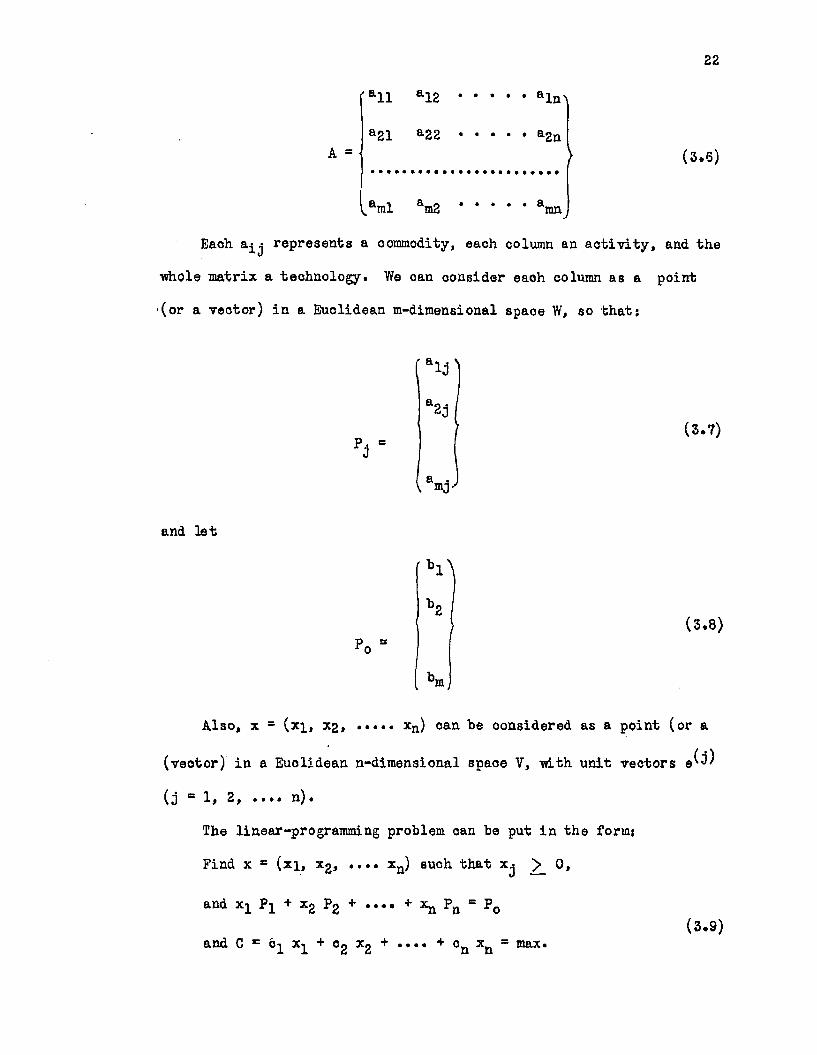
22

(all a12

a21 a22A =

aln^

a2n(3.6)

\_ainl am2 ......... amn,

Each represents a commodity, each column an activity, and the

•whole matrix a technology. We oan consider eaoh column as a point

(or a vector) in a Euclidean m-dimensional space W, so that:

a2j(3.7)

and let

Po =(3.8)

'Hi

Also, x = (x]_, X2, xn) can he considered as a point (or a

(veotor) in a Euclidean n-dimensional space V, -with unit vectors e^^

(j “ 1, 2, .... n).

The linear-prograraming problem can be put in the form:

Find x = (xi, xg, .... xQ) such that x^ >_ 0,

and xx Px + x2 P2 + .... + ^ PQ = P0

and C = b^ x^ + Cg Xg + •••• + cQ xQ = max.(3.9)

23

Each one of the vectors Pj can be viewed as the image in W of the unit vector e^) in V, transformed to W by a linear transformation L

so that;

L (e^)) > (3.10)

A transformation T (or a mapping of points from one space to

another) is said to be a linear transformation if;

I ( a x + b y) 5 a I (x) + b T (y) for all points x, y and real numbers

a, b. In other words it should have the additive property;

T (x + y) = Tx + Ty

and the homogeneity property

T(ax) = aT(x)

Concerning again equation (3.10), if g(^) (i = 1, 2, ....m) is a

unit veotor in W, then Pj can be expressed in the form;

Pj = Z. aij g(i) = L(e^)) (3.11)J i«l J

where a ^ are scalar quantities (which is the definition of Pj)

Equations (3.10) or (3.11) completely define the image in W of any

point x in V since x can be expressed as a linear combination of the

unit vectors;

n . .x = 21 Xj e'J' where Xj are scalar quantities (3-.12)

n nU*) = £! x j L ( e ^ O = 2 1 x j pi “ P0 <3*13)0=1 j=l J

Therefore, we can say that the matrix of coefficients A defines

a linear transformation of a point x (xj_, xg, ...., xn) in an n-

dimensional space V to a point P0 in an m-dimensional space W (p0 is

24defined by equation (3.8))*

The linear programming problem oan be put in this form:

Find the point x in the positive half-space of V suoh that

■where P0 is in W and C(x), a linear function of x, is a max

In matrix notation the problem can be put in the form:

(3.14)

Maximize C = cx (3.15)

•where C is the scalar produot of the two n-veotors o (l.n matrix)

and x (n.l matrix).

Subject to the conditions that:

l) A H elements in x are non-negative

where A is an m.n matrix and F0 is an m.l matrix (or vector). If

m = n and the set of m equations are independent, then, if any solu­

tion exists, it will be unique, that is to say, there is only one

point such that:

If m < n, there will generally be more than one solution, perhaps

an infinity of them. We will call the set of all solutions satisfying

both 1) and 2) S.

Theorem (l) The set S of all points y in V having non-negative coordin­

ates and such that L(y) - P0 is either null or a convex set.

A convex set is a collection of points such that if v and w are

any two points in the collection, the segment joining them is also in

the collection.

2) Ax =.p0 (3.16)

L(x) = PQ

The segment joining two points v and w is defined byj

sv + (l-s) w given 0 < s < 1 (3.17)

Proof of the theorems The set S may be null, contain preoisely

one point, or more than one point. If S is null, then the theorem is

obviously true. If it contains only one point, then it is a convex

set since a single point is a convex set. If there are more than one

point in the set S then suppose that y^ and y2 are any two different

points in it. For 0 <_ s < 1,

L (syi + (l-s) y2) = s L y^ + (l-s) L y2

= s P0 + (l-s) P0 = P0

Therefore the segment joining y^ and yg a-lso satisfies the condi­

tions of the equations; hence it is in the set and the theorem is proved.

Theorem (2) x (xj_, x2, .... xn) is an extreme point of the set S if

and only if the non-zero Xj are the coefficients of linearly indepen­

dent vectors p^.

A linearly independent set of vectors (or points) P^, P2, ....

Pk is a set such that ri pi + rg P2 + P^ = O’, the null vector

(0 , 0 , ...., 0 ), for real numbers rlf r2, ...., r^ only if «= r2 ....

rk =

If P0 = xi Pi + x2 P2 + .... + xk Pk where Pp P2, .... Pk is a

linearly independent set, then the values of x^, x2, .... xn are unique.

If the vectors are in an m-dimensional space, then there oannot

exist more than m linearly independent vectors. A set of m linearly

independent vectors is called a basis of the space, in terms of which

every vector in the space can be uniquely expressed.

26

A vector in a linearly independent set oannot be expressed in

terms of the other vectors in the set.

The theorem is proved in this sequence*

1. First it is proved that if Pg , Ps2, ... Pgm are linearly

independent, and if L (x) = Psl .... + 7 Psm = pQ, then x is an

extreme point of the set S. Suppose it is not, then it can be

expressed in the form

x = r x^1) + (1-r) x(2) (3.18)

■where 0 £ r £. 1 and *U), *(2) are two points in the set*

Sinoe the coefficients of PS7n+i, ...., Psn vanish, and since

r, (1-r) and all the coordinates of x, x^), and x^2) are non-negative,

then the coefficients of the same (m-n) vectors vanish in the expression

of x(l) and x^2). Therefore, P0 could be expressed in terms of the m

linearly independent veotors in three ways, which is contradictory to

one of the properties of independence. Hence x * x(-0 = x(^)( and x

would be an extreme point of the set S.

2. It is then proved that if x is an extreme point of S, then

the vectors in which P0 is expressed are linearly independent and are

at most m.

Suppose Ps , PSg, .... pSp are such that

PZ- xi Ps, = po (3*17)i=l i

If they are not linearly independent then there exists a linear combina­

tion of the P„ such thatsip _ .22 ri Ps = 0 where r ^ f 0 for all i = 1, ...., p. (3.19)i-1 1

Therefore, for any positive constant k, by (3.17) and (3.18) we

have*

Po = 1 *i P., ± k Z *i p,. - £ (*i ± to-i) PE.i=l 1 i“l i i=l i

Since x^ 2. 0, k can be chosen so small that both x^ + k r^ and

x^ - k r^ are positive for all i. Then

x U ) * (Xl + k r j , .......... . xp + k rp> 0 , . . . ., 0 )

x(2) = (Xl - t r i J ......... , xp - k rp, 0, ......0)

are both points in the set S. But since x = l/2 x(^) + l/2 x ^ ) » then

it could be expressed in terms of two other points, which is contrary

to the assumption that it is an extreme point. Therefore Ps , Ps , . • .,X 2Ps are linearly independent. As a consequenoe, p must be equal to or

less than m.

Theorem (3) A linear functional C defined on a convex polyhedron S

takes its maximum or minimum at an extreme point of the convex set. If

it takes on the max. (or min.) at more than one point, then it takesihe

same value over the whole convex set generated by those particular points.

A functional is a real valued function defined on an n-dimensional\

vector space. It may also be considered as a transformation which takes

the points of an n-dimensional space into a 1-dimensional space (the real

line), therefore the definition of linearity in a transformation applies

to it.

A convex polyhydron is a convex set which may be generated from a

finite number of points.

28

It should be noted that the set S is a convex polyhedron. It has

a finite number of extreme points since there can be no more than (-■).mProof of the Theorem If x, the point -which satisfies the maximality

condition, is an extreme point, then the first statement of the theorem

is true; if it is not, then it can be expressed as a linear combination

of other extreme points.

r rx * Z1 Gi where 0 < s^<: 1 and Z s. = 1

i=l i=l 1

Sinoe C is linear, then its maximum,

r r rc (x) - C ( £ H H ) s L Si C (Ai)< Z Si C Up)

i=l i=l i=l

where C(Ap) is the greatest of all the C(Ai)r

Therefore C(x) < C(Ari) T s, = C(An)p i*l p

Since C(x) is a maximum then C(x) = C(Ap) and C(Ap) is a maximum

also.

Nowr

x= S i “l &1 ‘ *» AP + "7 t Ei1 lC I

Where I is the set of all points i (l, 2, 3,...., r) except i = p

5P i€ i

C X*SPAr> “ C ( £ Si V F P i€ I

C(x) - A C(A ) = Z n C ( A i ) < Z si C(Aq) = C (AJ H «iP i d i« I iel

29

•where C(Aq) is the greatest of all C (A^) where ie I

Since C (x) = C (Ap) and Sj_ e 1 - s_ic I

then C(x) (l-sp)< C(Aq) (l-sp).

But C(x) is a max., then C(x) = C(Aq), and C (Aq) is a maximum

also. Similarly every extreme point which enters in the expression of

x can be proved to be a maximum. Therefore, either x is an extreme

point, or it can be expressed as a linear combination of extreme points

each of which is a maximum.

A similar procedure can be followed to obtain a proof when C is

to be minimized.

If C takes on a max. or min. for more than one extreme point, then

any point x in the set formed from these points can be expressed thus:

P px = Z. As where 0 £ s, S 1, s. = 1

i-i i=i 1

and A^ are the extreme points. If M is the value of max. G

P p pC (x) = £ si C (Ai) = £ M = M £L s , = M

i=l i=i i=i

and the theorem is proved.

The simplex method consists in finding any extreme point of the

set S (defined by equation 3.14). This extreme point will be a linear

combination of m independent vectors of the n Pj'sj so any m such

vectors (which will be called the basis) can be chosen to form a first

(basic) solution. This solution can be checked for optimality. If it

is found to give a max. for C, then it is the final solution} otherwise

30a vector is sought, which is not in the basis, and which if entered

into it will increase the value of C. One of the vectors in the

basis will be removed so that a new point will be reached which is

both an extreme point and having a higher value of C.

Suppose that the initial extreme point was expressed as a

linear combination of the first m vectors, thus}

mZ Xi ?i = Po (3.20)isl

zQ will be defined bysm£ CA = (« C) (3.21)i=l

The vectors Pm+2> * * * * Pn can e3T>ressed as follows*

£ yio Pi * PJ (S-22>

where j = m + 1, m + 2, . . . .,n and y ^ is the coefficient of the

vector of the basis in the expression of the vector

z. will be defined by*Jm^ ^ii = zi (3.23)•‘• J O J

Theorem (4) If for any fixed j, the condition o^ > Zj holds, then a

subset of S (i.e. a set of solutions to (3.14)) can be constructed such

that z ^ zQ>

Multiplying (3.22) by 6 and subtracting it from (3.20), and multi­

plying (3.23) by 0, subtracting it from (3.21), and adding 0cj to its

both sides, we get*

31

mZ (Xi - 0 yij) Pi + 9 Pj = Po (3.24)i=l

mand jT (x^ - 0 y.^) Ci + 9 Cj c z0 + 8 (c^ - z^) = z' (3.25)

Since Cj y z^ (i.e. c^ - z^ ,> 0), and since x^2l 0< then if there

exists a set of values of & (0 j£O) such that (x. - & y. .) remain non-x 10negative, then we will have mother set of solutions with z1 > z0, and

the theorem is proved.

Let us call the vector (or one of the vectors) Pj for which

Cj > Z y We have two cases:

1. All yik<_0. By (3.24), for any positive value of 0, all

the coefficients of will remain positive. Therefore 0 can assume

any value up to infinity and the maximum value of C will be infinity.

2. Some y ^ > 0 . We can introduce P^ into the basis, but to keep

the coefficients (x^ - 0 y^^) positive, we chose 0O (the upper limit

of the set of 0) such that:

eo = m i n J ^ (s>26)^ik

Suppose this occurs as i - r, then the coefficient of Pr

xr “ yrk * Yrk “ 0 (3.27)

and the vector Pr can be removed from the basis. Therefore the point

P0 is expressed as a linear combination of m vectors whose independence

can be proved, and the new point is an extreme point of the set S.

Z x' p. = P0 (3.28)i<F I

32

where I is the set of all i = 1, 2, ... m with the exception of i = r

and with i = k added and -where

ix.l X. -1 yrk * yck r°r a11 1 t k (3.29)

and

(3.30)

(Jtr. „ nan _*i_ „ yrk n k 0

Alsom

pj s z yij pi (3-22)i=I

m

i=l yij Pi " ® pk + ^ Pk

m ( myij pi - ® 2 L yik Pi + 0* Pk

i=l J i=l

m t* lyu ' 9 W pi - 9’ pk = f tl yi3 h

Sinoe Pr is removed from the basis, its coefficients in the expres­

sion of the vectors P. must disappear; hence,

yrj - 6 ’ yrk = 0

i e i1 = yrkyrk

Therefore y ' = y , <= III . y i / k (3,31)J J yrk

aQd , , y .yk i = 8 = ^ (,.»)

33

If more than one P. satisfied the condition o. z., then tov J Jobtain the maximum increase in Z in one move is chosen such that*

9ok K - ziP = naxSince this involves additional computational difficulty is

chosen such that (c^ - z^) is a max.

If at any step, no c., > z ., then no other solution exists foro J■which the value of the functional C is greater than the final one,

and the solution reached is the optimum.

If at this final point, some cj = Z y the corresponding ?■ repre­

sents vectors which, if introduced in the basis, will give solutions

having the same value of the functional C. These are alternative

optimum solutions which, if found, can give the management a chance

to select one of several equal programs. Also next and third best

programs can be determined, so that they can be considered in case

difficulties arise in the execution of the optimum program.

In the simplex method, one proceeds by iteration from one extreme

point to another, putting one vector in the basis and removing another,

according to the above-mentioned criteria. In each step the value of

C increases, (except when the coefficient of the variable to be removed

from the basis is equal to zero; and any difficulty arising from such

a situation can be solved by the € -technique, which is described later).

Therefore no value of C will recur, and we are always choosing new

bases or extreme points. Since, as mentioned before, there is a finite

number of extreme points, then the iterative procedure will eventually

terminate at the point where all c^ ?Lzy

34

If the functional C is to be minimized a simple procedure is

followed. Suppose

C = c. x- + o„ x_ + . . . . + c x = min.1 1 2 2 n n

multiply C by -1, and define C’ by

C = - o, x. - c, x - i . , . - c x1 1 2 2 n nr

Minimum'C = maximum C1 (Algebraically)

The problem then can be solved in the normal way with the condi­

tion that C* is to be maximized instead of minimizing C.

Degeneracy and the e -technique;

At a certain step of the simplex procedure, the vector P0 may be

expressed as a lineer combination of less than m vectors, i.e. the

coefficients of one or more P^ are equal to zero. This situation is

termed "degeneracy". When degeneracy occurs, more than one vector in

the basis will have zero coefficients in the expression,

m2=. (xj. - 8 0 yik) Pi * 9 Pk = P0 (3.24)i=l

putting j = k.min xiThat is = i --- is the same for more than one i and a tie

0 yikwill occur. This situation is resolved by what is called the -technique.

The vector PQ is expressed thus;

m n2 7 Uj. + 2. ^ - e0 yik) Pi + pk = p0 ( * ) (3.33)i=l j=l

where £ is an unspecified very small positive number.

Similarly

m nZ T (*i+ £ y y + 90 ylk) 0 - e 0 = c£ (x) + e (ok-z ) (3.34)i=l . j=l

In this oase 9 = "i*1 t Z £

35n

I'

No tie will occur in this oase because each one of the for

je I (where I is the set of basis vectors), i.e. for j = i, appears

only as a coefficient of P ^ The coefficient of Pi in the expression

of P0 is s

*i + «•> Z ^ yij i not£ I

xiSo if there is a tie occurs in min, ----, the next step is to tryyik 2

min if there is still a tie try "“f11 c ^ 2 , and so on. A1 yik - j i t

point will certainly be reached -when this ratio will be smaller for

one Pi than all others, and this P^ will be removed from the basis.

It oould be noticed that the e 's do not have to be written if the

vectors Pj are arranged in a oertain order which is not changed all

through the steps of the solution.

If the initial problem isj

n5s. P0 Xj > 0 Po, Pj is m-dimensional

it can be put in the formn+mz

£ Pj + i=n+1 Xi Pi = Po (3*35)

where P^ are m-dimensional unit vectors. The matrix formed by the m

vectors Pi will be the identity matrix I.

36

1 0 . . 0 0

0 1 0of order m (3.36)

,0 0 . . 0 1

These P£ can form a basis for the initial solution, in which the

a^j in the expression of Pj (equation 3.7) will be the y^j in equation

(3.22). The P^ are called slack vectors and the x^ slack variables.

If the initial problem is:

Z pj ’ p°j-i J

The problem still can be put in the form (3.35), where the vectors

Pj_ have an exceedingly high price (m ) on them, so they will be gotten

rid of in the final tableau. The advantage of this procedure is to be

spared considerations of independence or the existence of a feasible

solution. The P^ in this case are called dummy vectors and the x^

dummy variables.

Numerical Example

The following extremely simple example is presented to illustrate

the simplex method#

maximize C = 2x^ + x2 such that X1 < 4

(3.1a)(3.2a)

x2 7 (3.3a)4x2 < 20 (3.4a)x2 2. 0 (3.5a)

Put 3.1a, 3.2a, 3.3a in the form:

37

x- + x4 = 4 (3.6a)x2 + x4 = 7 (3.7a)

X 1 + Xg + Xg = 6 (3.8a)

where xg, x4 and xg are slaok variables

The last three equations are entered in a table suoh as shown in

table I. Each step in the calculations is represented by a tableau,

therefore tableau (a) represents the first solution. In this solution

Pg, and Pg, the slack vectors, form the basis, and,5

P0 = E Xi Pi = 4P, + 7P4 + 20 P5 i=3

5C = z0 = 21 Ci » 0

i=3

5 5PJ = £ , yi3 Pi ■ H j pi

where a- * are the coefficients of x.JFor example

Pi = l.Pg + 0.p4 + 3.P5

Also s. is defined by,J 5

z3 = X yU °i

This is more clearly illustrated in table I* which represents in

symbols tableau (a) of table I.

It was found in the first tableau that P^ gives the most negative

zj = cj = -2, therefore Pi is the vector to be entered in the next basis.: 20Dividing each x^ by the corresponding y4g, we get 4, + 00 and y for Pg,

P4 and Pg respectively. The minimum of these values is 4, so Pg is to

be removed from the basis*

38Table I

Numerical Example of a Simplex Solution

Cj 2 1

* Po P3 P4 P5 Pl ?2

- P3 4 1 1

a P4 7 1 1

P5 20 1 3 4

2 j.. .

zr cj *■2 -1

z P1 4 1 1

P4 7 1 1

b - P5 8 -3 1 4

zi 8 2 2

zr°j 2 -1

z Pl 4 1 1

P4 5 3/4 1 -1/4

c Pz Z -3/4 1/4 1

zd 10 1 1/4 1/4 2 1

zr°3 1 1/4 1/4

39

Table I'

°0 °3 c4 °5 C1 °2

*Po P3 P4 Pl p2

°3 p3 x3 y33 y34 y35 y31 y32

a °4 P4 x4 y43 y44 y45 y41 y42

c5 P5 x5 y53 y54 y55 y51 y52

ZJ

zr°j

40

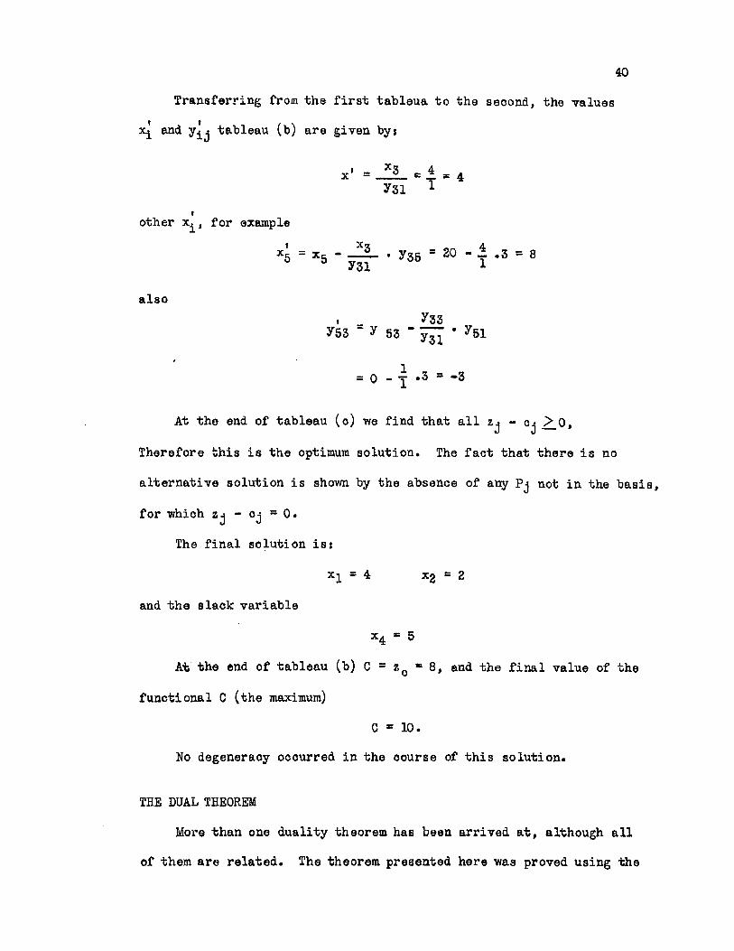
Transferring from the first tableua to the second, the values

x^ and y]^ tableau (b) are given byj

Y« - x3 _ 4 _ ,x ---- - _ - 4y31 1

tother x., for example

x

also

*6 ° 16 ‘ Ti!" ' yss = 20 ' T '3 * 8

. ^33y53 “ y 5 3 " ' y51

= o - T *3 = *3

At the end of tableau (o) we find that all - Cj > 0.

Therefore this is the optimum solution. The fact that there is no

alternative solution is shown by the absence of any Pj not in the basis,

for which zj - oj = 0 .

The final solution isj

= 4 x2 - 2

and the slack variable

x4 ■ 5

At the end of tableau (b) C = zQ - 8, and the final value of the

functional C (the maximum)

C c 10.

No degeneracy occurred in the course of this solution.

THE DUAL THEOREM

More than one duality theorem has been arrived at, although all

of them are related. The theorem presented here was proved using the

simplex method by Orden and Dantzig.*'

Consider the two problems}

Problem la Minimize f “ ox where f is a linear form, o a known

n-component raw vector, and x a column vector, subject tos

1. Ax = b (3.37)

2. *j£.0 (3.38)

where A is a known m x n matrix, and b is a known m-dimensional column

veotor.

Problem lb Maximize g = wb where w is an m-dimensional raw veotor,

and g a linear form, subject tot

3. wA<_c (3.39)

w is not restricted as to non-negativity.

The Dual Theorem (l) If a solution to either la or lb exists and is

finite, then a solution to the other also exists and min f = max g

(3.40)

Proof Let

x' be the m-vector, which is the value of x that gives min. f

c’ the m-veotor of the terms of c associated with the components

of x*

B an m x m matrix whose columns are the basis in the final

simplex tableau expressed as they appear in the matrix A.

This is a submatrix of the matrix A.

y = the m x n matrix of the final tableau

TT Dantzig, G. B., and Alex Orden. "A duality Theorem Based on the Simplex Method,11 "Symposium on Linear Inequalities and Programming, (mim.), Washington, D.C., June 14-16, 1951.

42

A = BY (3.41)

b = bx' (3.42)

f min = e'x* (3.43)

In the final tableau,

o'y - o <. 0 (3.44)

Let w* be an m-dimensional raw vector defined byj

w' * o* B"1 (3.45)

B' is the inverse of B

Then by (3.45), (3.41) and (3.44) we have,

w> A - o = o* B“ A - c “ o' y - c 0 (3.46)

i.e. w ’ satisfies the linear inequalities 3. of problem lb.

Therefore when problem lb has a finite solution, then lb has solutions.

Also by (3.45), (3.42) and (3.43) we have,

g (w)- w' b * c* B** b = c* x‘ = min f. (3.47)

For any x that satisfies (3.37) and every w that satisfies (3.39),

w A x = w b s,g (w) (3.48)

But from

w A x £ . o x = f (x) (3.49)

Therefore g (vr),< f (x) for any feasible value of x and w, i.e. max.

g min. f

But from (3.47) g (w) * min f

g (w) - max g

and max. g = min. f which proves the theorem.

Another duality relationship will be stated without proof, this

has been first stated by Von Neumann.

43Problem 2a

Maximize f - c x (3.50)

subject to

Ax b (3.51)

(3.52)

Problem 2b

Minimize g = wb

subject to

w A — c (3.53)

(3.54)w i ) 0

Dual Theorem (2) If a solution to either 2a or 2b exists and is finite,

then a solution to the other exists and

The definition of the terms in these two problems is the same as

in the previous ones. The difference between the 2 theorems is that

in problem 1 a the relationships are in the form of equalities, while

in 2a they are inequalities. Also in 2b the restriction of the non­

negativity of w is added.

The dual theorem, has many applications. It is used when the

simplex technique is applied to game theory problems. Also it is

used in the conversion of the linear programming problem into a problem

involving the solution of linear inequalities.

Applications of the Simplex Method

Obher than the solution of the linear programming problem, and

establishing the relationship between it and its dual, the simplex

method has other important applications some of which will be discussed

in this section.

min f = max g (3.55)

44

1. Solution of System of Linear Inequalities

There are more than one approach to the solution of this problem

by the simplex method, only one of these will be presented here.

Consider this set of linear inequalities!

A x 2L b (3.56)

A is m.n, x is n.l and b is m.l

To convert this set into a linear programming problem,

1. The non-negativity restriction is added by rewriting,

x = yj " yn+j (3.57)

where both yj and ya+j are non-negative. The new set will be,

(Al-A)</£fc (3.58)

y = 1, 2, ...*, 2n.

2. An optimization criterion is added by introducing dummy varia­

bles which are to be eliminated in the final solution. Let this be a

positive m-oomponent raw vector (v) with coefficients equal to unity.

Therefore the problem reduces to the problem of finding a solution to:

(A | - A ) I) (y I v) < b (3.59)

where I is an m.m unit matrix, which maximizes

f =-M(v) (3.60)

where M is an arbitrarily large positive number.

If such a maximum exists, at which f = 0, then this will be the

solution to the set of inequalities (3.56), since all the introduced

dummy variables v will be eliminated. Otherwise, no solution for the

set of inequalities exists.

Other approaches of solving linear inequalities by the simplex

method can be made by maximizing a function g defined by

g = yi + y2 + ...... + y2n (3.61)

45

instead of introducing dummy variables, or by applying the above-

mentioned dual theorem.

2. Solution of Game Problems^'^*^

It was first pointed out by John von Neumann that a game problem

can be reduced to a program problem. Consider the zero-sum two person

game for which the payoff matrix is the m.n matrix A, or

Suppose that the maximizing player engages in a mixed strategy given

by the n-oomponent veotor x, or (x^) suoh that

nZ 3Cj “ 1 (3.62)0=1

and

x-j 0 (3.63)

This player's expected payoff (M) will be,

min 2- , . , .M = Z. a^j xj (i a 1, 2, ...., m) (3.64)j=l

Therefore his strategy would be to choose x such that M is a maximum.

Suppose this minimum occurs at some i = k

nZ aij x. > M (3.65)

The equality sign holds at i = k

The problem is then to find a solution (x) to the system of inequalities

(3.65), or put in matrix form:

A x ) M , (3.66)

1 Gale, D., Kuhn, H. W., and Tucker, A. W., f,Linear Programming andthe Theory of Games," Koopmans, T. C., Aotivity Analysis of Produotion and Allocation, Ch. XIX. Wiley, N.Y., 1951.

2. Dantzig, G. B., ,kA Proof of the Equivalence of the Programming Problem and the Game Problem” Koopmans, T. 0. Op. Cit., Ch. XX.

3. Orden, A., "Application of the Simplex Method to a Vanity of Matrix Problems," Symposium on Linear Inequalities and Programming, U.S.A.F. Project SCOOP No. 10, pp. 28-50.

■which will maximize M. Substitute x for x suoh that,

x M = x (3.67)

and the problem reduces to a linear programming problem in the form:

Find x such that

x A > l (3.68)

and

£ X = 2. x/m = i/m = min. (3.70)

where

xj> 0 (3.71)

Because of the non-negativity restriction in the linear program­

ming problem, the conversion of the original problem into it is only

valid if M i s known to be positive. If all the elements in the payoff

matrix are positive, then M will be positive, otherwise, they can all

be made positive by the addition of an appropriate constant to all of

them. This will not affect the mixed strategy x.

3. Solution of Some Matrix Problems

Orden"^ showed the simplex method can be applied to solve such

matrix problems as:

a. Matrix inversion

b. Linear Simultaneous Equations

o. Basis Transformation

d. Evaluation of Determinants.

These will not be discussed in detail.

47

Solution of Large Scale Problems^*^

Although the simplex method is very effective in solving an

average size linear programming problem, yet the computations involved

in it become prohibitive "when the number of variables is large. Systems

of 100 equations and any number of unknowns have been successfully

solved at Rand Corporation in about five hours with a special simplex

code . Due to technical difficulties, a system involving 200 equations

could not be practically solved on the machine, although such a system

is not unusual in practical situations.

Fortunately some linear programming problems have certain properties

that makes them easier to compute even if they are large scale problems.

Computations can be greatly reduced if the problem can be put in the

form of a transportation model, which will be discussed in the next

chapter. Three other forms will be discussed in this section which

can render computations easier, namely, upper bounds, secondary con­

straints,' and block triangularity, the latter being the general case.

These forms will be presented very briefly.

1. Variables with Upper Bounds

Suppose that many, or all, variables in the initial set have upper

bounds, the effect will be to increase the number of restrictions by

one for each such upper-bounded variable. An upper bound will be of

the form0 < xj <T (3.72)

Dantzig, G.' B., ’’Upper Bounds, Secondary Constraints and Block Triangularity in Linear Programming,’’ Econometrica, Vol. 23, Wo. 2, pp. 174-83, April, 1955.

2. Dantzig, G. B., "Status of Solution of Large Scale Linear Programming Problems,” Rand Corporation Research Memorandum RM-1375 U.S.A.F. Project, 9 pp.

3. Ibid., p. 5.

48

The simplified procedure consists in solving the problem as if these

upper bounds do not exist, until one, or more, variables in the basis

assume values that violate (3.72). Suppose that the variable which is

introduced in the basis xs violates (3.72), that is,

xs ** 9 > dB (3.73)

and/or one (or more) of the variables already existing in the basis

assumes a value which exceeds the upper bound, that is, changes from

< d3 to

Xj + 0 yj > dj (3.74)

In this case the permissible range of 9 should be reduced such that all

the variables in the basis will satisfy relation (1). Using the upper

bound of the range of 9 one (or more) of the variables in the new basis

reaches its upper bound, let this variable be x .. This variable is

then replaced by (d . - x^) and the new problem involving the new

variable and a new constant vector is solved for optimality.

Using this method,the addition of more inequalities to the initial

matrix is avoided.

2. Block Triangularity

Block triangularity means that if one partitions the matrix of

coefficients of the technology matrix into submatrices, the submatrices,

(orblocks) considered as elements form a triangular system,^-

All

A2i H z (3.75)

H i H z " ' H i1. Dantzig, G.Bi, "Upper Bounds, Secondary Constraints and Block

Triangularity in Linear Programming," Econometrics, Vol. 23, No. 2, p. 176, April, 1955.

49

A special case of block triangularity is found in the linear

dynamic model (3.76) developed by Von Neumann,^ in considering a

constantly expanding economy. In this model A is the submatrix of

coefficients of activities

A

-B A

-B . (3.76)

• •

-B A

initiated in period t, and B is the submatrix of output coefficients

of these activities in the following period.

If the diagonal matrices (A) in the triangular system are square

non-singular, the basis is referred to as a square block triangular

basis. If a model is square block triangular of the type (3.76), then

it is easy to handle since it is only necessary to find the inverses

of the diagonal submatrioes, and since in one iteration it is only

required to modify one of these smaller matrices. Although most bases

taken from block triangular systems are not exactly like this ideal

form, they are very close to it. A slight transformation of the matrix

might put it in the square triangular form. The inverses of matrices

might not be necessary to work -with if they are composed largely of

zeros of no obvious pattern.

3. Secondary Constraint

Oftentimes a subset of the group of restrictions form what is

Y. Von Neumann, John, "A Model of General Economic Equilibrium,"The Review of Economic Studies, Vol. XIII,(1945-46).

50

called secondary constraints. The main property of these is that only

a small subset of the restrictions is aotive. If the restriction is for

example of the form

nZ aij xj + xn+i = bi (3*77)

■where x ^ is the slack variable, then it is considered active -when the

slack variable is equal to zero. The way to solve this kind of problem

is to disregard the seoondary constraints and solve the problem to

satisfy the other restrictions only. The system is then expanded to

contain the secondary constraints, and the old solution is no longer

optimal. An initial basis for the new problem can be obtained by

augmenting the final basis of the smaller problem. The result will be

a basis in which not all the variables associated with the secondary

constraints are positive. The Dual %thod^ may be employed in this

case since in that particular form it takes care of variables without

the non-negativity restriction.

APPLICATIONS OF LINEAR PROGRAMMING

The linear programming problem as a model has applications in a

variety of practical situations. Following is a list of examples of

the general areas where it can be applied. The objective in all these

cases is the optimization of a certain criterion.

1. Determining quantities of each ingredient in a product mix.

2. Distribution of jobs over machines, and of employees over jobs.

3. Space and time utilization, for example in storage, shipment,

transportation, etc.

4. Allocation problems.

1. Supra, p. 39

51

5. Evaluation problems (for example of sales plans, inventory

strategies, effect of new equipment, etc.)

This is apart from the special applications discussed in the next

chapter. A great deal of success has been achieved in applying the

linear programming model to the first category of these problems, namely,

the optimum product mix. An example of such application is presented

below. This study was made by Charnes^ and others on the optimum

aviation gasoline blends. The problem was to find the quantities of

each of four components in three aviation and one automotive gasoline

blends such that a certain profit function is maximized. At some

intermediate stage of processing, the crude oil is divided into various

products, usually determined by boiling properties. The gasoline pro­

ducts at this stage areusually called straight-run gasolines. The

components in aviation gasolines are certain straight-run gasolines,

catalytically cracked gasolines and special components synthesized

from other refinery products such as alkylate and isopentane.

Certain specifications of the blends present restrictions on the

blending ratios. The two main specifications deal with ignition pro­

perties, as measured by octane ratings or performance numbers (PN) and

volatility as measured by Rein Vapor Pressure (RVP). The property of

the blend (its performance number or its RVP) depends on the amount of

eaoh ingredient in the blend and its property. The three aviation

gasoline blends are'80L, 9l/96 and 100/130, where 80, 91 and 100 repre­

sent the lower limits of the performance numbers of the three mixes

respectively. These can be denoted by M, N and Q respectively. If A,

TT Charnes, A., Cooper, Yf. VI., and Mellon, B., "Blending Aviation Gasolines", Econometrios, April 1954.

52

B, D and F represent the components: alkylate, catalytic gasoline,

straight-run gasoline mix and isopentane respectively, then:

94 Am + 83 Bm + 74 DM + 95 FM > 80 M (3.78)

where Ajj, Bjj, % and Fjj are the amounts, in Barrels per day of each

component in the blend M, and the ooefficients are the input-output

relationships. The coefficient of M (80) is the least permissible PN

for the blend M. Also,

107.5 An + 93.0 BN + 87.0 DN + 108,0 FN > 91 N(3.78)

and 107.5 Aq + 93.0 B + 87.0 D + 108.0 Fq >. 100 Q

Three additional inequalities can be written to represent the restric­

tions on the R.V.P. of the blends. The maximum R.V.P. is taken 6.9 for

all grades. Therefore,

5.0 Am + 8.0 Bm + 4.0 Dm + 20.5 FM < 6.9 M

5.0 An + 8.0 Bn + 4.0 DN + 20.5 FN <6.9 N (3.79)

5.0 Aq + 8.0 B + 4.0 Dq + 20.5 Fq <6.9 Q

where the ooefficients are also input-output relationships.

By definition,

M = AM + % + Dm + Fm

N = Ajj + Bjj + Dr + Fr(3.80)

5 - A, + B, + D(J + Fq

z ^ a + b + d + f - m - n - q

Z is the quantity of the premium automotive gasoline blended of what

is left from the aviation gasolines.

There is a steady rate of input of all the components. This

gives four additional equations:

53

A = Am + An + Aq + Az= 3800

B = % + % + bq + Bz= 2652(3.81)

D = % + Dn + Dq + Dz= 4081

P = FM + FN + Fq + Fz= 1300

■where the numbers at the right hand side of the equations represent the

flow of each component in barrels per day.

Using the relations of (3.80), and applying algebraic simplifica­

tion, the relations specified in (3.78) and (3.79) can be written in

the form,

14 Am + 3 % ’ 6 % + 15 fm £ 0

16.5 Ah + 2 Bn - 4 Dn + 17 Fn > 0

7.5 Aq + 7 BQ - 13 Dq + 8 Fq > 0(3.82)

1*9 Ajj - 1.1 Bjj + 2.9 Djj - 13.6 Fj j> 0

1.9 Ajj — 1.1 Bjj 2.9 Djj - 13*6 Fjj ^ 0

1.9 Aq - 1.1 bq + 2.9 Dq - 13.6 Fq > 0

Each one of the variables in the relations (3.81) and (3.82) are non­

negative. Inequalities (3.82) can be turned into equalities by intro­

ducing slack variables whioh can assume only non-negative values and

which are to be subtracted from the left hand side of the inequalities.

The problem now is to find values for the variables which maximizes a

profit criterion. This profit criterion R can be written.

R » 4.96 M + 5.846 N + 6.451 + 4.830 Z - 0.05177 M - 0.409416 (N + Q)

- 0.281862 Z (3.83)

where positive coefficients represent receipts in dollars per barrel

and the negative coefficients stand for the cost of tetraethyl lead

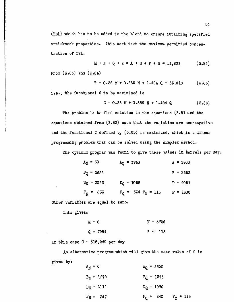
54

(TEL) -which has to be added to the blend to ensure attaining specified

anti-knock properties# This oost is at the maximum permitted concen­

tration of TEL.

M + N + Q + Z = A + B + F + D = 11,833 (3.84)

From (3.83) and (3.84)

R = 0.36 M + 0.889 N + 1.494 Q + 53,818 (3.85)

i.e., the functional C to be maximized is

C = 0.36 M + 0.889 N * 1.494 Q (3.86)

The problem is to find solution to the equations (3.81 and the

equations obtained from (3*82) such that the variables are non-negative

and the functional C defined by (3.85) is maximized, which is a linear

programming problem that can be solved using the simplex method.

The optimum program m s found to give these values in barrels per day

A n = 60 A q = 3740 A = 3800

B q = 2652 B = 2652

% = 3023 D q = 1058 D = 4081

Fn * 653 Fq * 534 Fz =113 F = 1300

Other variables are equal to zero.

This gives:

M = 0 N = 3736

Q = 7984 Z = 113

In this case C = $15,249 per day

An alternative program which will give the same value of C is

given by:AN = 0 Aq = 3800

Bn = 1279 Bq = 1373

D n = 2111 D q = 1970

Fn = 347 Fq = 840 Fz = 113

55which gives j

N = 3737 Q = 7983 Z = 113

Other examples of the use of linear programming in refinery

problems can be found in a book written by Symonds1.

U Symonds, Gifford H., Linear Programming: The Solution ofRefinery Problems, Esso Standard Oil Company, New York, 1955.

CHAPTER IV

SPECIAL CASES OF LINEAR PROGRAMMING

Some forms of the linear programming problem make it possible to

use simpler computing procedures than the simplex method. These are

special cases of the general problems ■which contain added restrictions.

With some of these forms large scale problems were solved in relatively

short periods of time. A number of these special cases will be dis­

cussed in this chapter, namely, the transportation, assignment,

traveling-salesraan, network and caterer problems. The traveling-

salesman problem is represented as a special case of the assignment pro­

blem, which, in turn, is a special case of the transportation problem.

THE TRANSPORTATION PROBLEM

Definition

Consider the problem of transferring quantities of a certain com­

modity from a number of origins to a number of destinations such that:

1. The available quantity from each origin and the required

quantity at each destination are specified, and the total at origins

is equal to the total required at destinations; and that

2. There is a known cost for the transportation of the oommodity

from each origin to each destination.

The problem is to determine the quantities to be transported from

eaoh origin to each destination (these quantities could only be non­

negative) such that the total cost of transportation is minimum.

56

57The same problem stated mathematically is:

Minimize C = c^-

where

i = 2,..... , m,

3 ~ 1» 2,«•■•«, n,

and c^j are known real numbers, such that, (m could be the number of

origins and n the number of destinations)

n£ ~ (i-1,... ,m) (4.1)3*1

mZ 1 xAi = b i (j=l,...,n) (4.2)i=l J J

where a _ and b^ are knovm real numbers and

xij > 0 (4.3)

This is a special case of the linear programming problem;

ij ^ 3Minimize C = -2T c. .. x .. (4*4)

such thatn. . dij xi3 “ ai 0*1

where di are known real numbers, andJ* Jxij > 0

with the additional restrictions that;

dij = 1 (4.5)

and the restriction given by equation (4.2).

The nature of this problem makes it possible to use certain techniques

for its solution that are not usable in the case of the general problem.

The data are usually put in the form of table II, p. 59.

The Simplex Method

Since this is a linear programming problem, it can be solved by

the simplex method after it is stated in terms of the single script

notation.

If the subscript f is put to represent ij such that

f = (i - 1) n + j (4.6)

where

f*- 2 **» Hj n + ly mn

(for example xp = - x(i-l)a+j) then the original equations (4.1)

and (4.2) can be put in the form

xi + x2 + ... + xn = a]_

xn+l + ••• + x2n = a2

=ai

x(m-l)n+l +*“ + x mn = am <4'

X1 + I n+1 + + x(m-l)n+l = bl

x2 +xn+2 + ....... + x(m-l)n+2 = b2

•»• *• •• = "bj

*n + x2n + xmn = \

These are m + n equations.

Due to the faot that

2 *i = z Z x!j = Z Z xij = £ bj (4.8) ^ J «j ^

then any of the a^ or b^ can be known if the rest of the (m + n)

and bj are known. In other words, one of the above (m + n) equations

in the relations (4.7) is dependent on the remaining (m + h - 1)

and only a set of (m + n - 1) equations could be independent.

Table II

59

Destinations

0rigins

D1 D2 Dn1Total

°1 X11 x12 Xij xln al

°2 X21 x22 X2j x2n a2

<>i xil ^ 2 Xi^ ^ n ai

^ 1 xm2 xmn am

Total bl b2 bi_ *n xijA

»1 D2 . ** Dn

°1 o n c12 cij cln

o2 021 °22 °2j c2n

Oi °il °i2 °i.1 °in

Om °ml °m2 °mj cmn

Data given ares a^, bj, and

Required; Xjj to minimize C = cjji»a

60

Putting the problem in vector notation, it m i l be

Minimize C = ^ Cf xj f

or

Mimize C’ = - 2 op Xf= Cf Xf (4.9)f f

such that

if Xf Pf = PQ (4.10)f

where PQ is the vector composed of the column of constants af, bj, and

Pf (originally Pf j) is the vector consisting of the column of coeffi­

cients of the variable Xf (see table III, p. 62). Since these coeffi­

cients are always unity and since Xf appears only in the equations

having as their right hand sides af and bj (f stands for ij), then

pf * p(i-l)n+j - % + vj (4-u >

where Uf is an (m + n) component unit oolumn vector having unity in

row i and zeros elsewhere, and Vj is same but with unity in row m + j

instead.

For example xg (which is originally xfg) appears only in the

equations containing a^ and and therefore Pg (originally Pfg) is

equal to TJi + V2«

It should be noted that each one of the Uf and the Vj is inde­

pendent of the others and cannot be expressed as a linear combination

of them.

Since the number of independent equations is (m + n - 1), then

in an optimal solution PQ is expressed as a linear combination of at1most + a ~ 1) Pf* °r "basis vectors Pr«

1. Supra, pp. 26 and 28.

61

Table III

Pf Expressed in Terms of and "Vj

^1 ^2 • * * ^n ^n+1 ••• ^(i-l)n+j ••• Pmn

Ui JJ-i U]_

TJ„

Vl

U4

u,m

al

a 2

ai

bl

b2

bj

The elements adding to P » are listed in its same column sot

pn+l " u2 + V 1

63

i » e»m+n-1

P0 ” xr (4 * 12)r=l

andm+n-1

C = X cr Xy (4.13)r=l

This can he made clearer if it is noticed, with reference to

table II, p. 60, that the n vectors P^, P2, Pn (i.e. P;q, P^g

P- n) contain n + 1 different unit vectors (Ui> Vj_, Vg, •••Vm)

and that each one of these P^ vectors contains a unit vector which is

not a component of any one of the others; in other words, these n

vectors are independent. Each one of the remaining groups of vectors

p(i-l)n+l,**#» p(i-l)n+n i,e* pil, ***» pin) where 1 = l* z> •••»

contains only one unit vector which is not included in the previous

group, namely, U^. Selecting one, and only one, vector of each of

these (m-l) groups provides the rest of the unit vectors required.

This gives a total of n + (m-l) i.e., (m+n-l) veotors forming a basis

in terms of which any vector can be expressed. If less than (m+n-1)

independent vectors are taken as the basis, some of the unit vectors

Uif Vj will not be included; thus expression of vectors containing

these unit vectors, as a linear combination of the components of the

basis, will not be feasible. This case, as in the general linear

programming problem, is called degeneracy.

Consider the basis consisting of P^, Pg, •••, Pr, ..., Pm+n-l>

where r = (s-l) n + t

thenm+n-1

pf = £ Yrf prr=l

63

= yir P1 + y2f ?2 + ••• + yrr pr + ••• + ym+n-1, f Pm+n-l

That is,

Vs + Vt = yif (^! + Vx) + y2f (Ux + V2) + ... + yrf (Uj. + Tj) + ...

+ ym+n-1 (Uu + V■where Uu and Vv are the and corresponding to the last vector in

the basis Pm+n-x.

Since Us in the left hand side of the equation can be only equaled

by the same Us at the right hand side and not by a linear combination

of other unit vectors (and the same for V .), then for the two sides of

the equations to be equal, coefficients yrj of the vectors should be

selected so as to leave only TJ = U8 and Vj = with coefficients of

unity. To obtain that,

1. A vector Pp = is selected from the set of vectors Pr

(the basis) such that = Us (i.e., s=l) and that is contained in

some other vector (or vectors) in the set. The coefficient of this

vector ypj is put equal to +1.

2. Another veotor Pq in the basis is selected such that its

Yj is the same as the component Vj of P , and that its is a oomponent

of another vector in the basis. Pq is given a coefficient of (-1).

Adding (+Pp) and (“Pq) will eliminate Vj.

3. The procedure is continued moving from a basis vector having

the same Uj_ (or Vj) as the previous one to another one having the

same Vj (or U^) as 01ira» until a basis veotor iB reaohed with

Vj = V .. The coefficients of these basis vectors are put equal to

+1 and -1 alternatively.

64

4. Adding all these vectors taking the signs in consideration

eliminates all the intermediate unit vectors, and thus only TJS and

V-t will remain on the right hand side.

5. Those vectors of the basis having (+1) or (-1) as coefficients

are called "stepping stones"'*’ since one steps from one to another to

evaluate a non-basis vector.

6. Other vectors of the basis are given zero coefficients.

7. The scpression of a non-basis vector P f in terms of vectors

in the basis is unique since the basis vectors are independent.

The reason why a non-basis veotor is expressed as a linear com­

bination of basis vectors is to evaluate it and see whether any increase

in profit (or decrease in cost) can be effected by its introduction to

the basis.

Letm+n-1

Zf = 21 yrf (4.14)r=l

Then if Zf - O f < 0, a possible increase in the value of C

(equation 4.13) can be obtained if Zf is introduced into the basis «

All non-basis vectors should be evaluated and the vector (Z^-bp which

is most negative is selected to be introduced in the basis. To obtain

(Zf-o]»), plus and minus signs are assigned to the prices (c^) associated

with the stepping stone vectors (Pr), and from the sum obtained by

adding the resultant values, c'f is subtracted, giving (Zf-o].).

Tl Charnes, A., and Cooper, W. W., "The Stepping Stone Method of Explaining Linear Programming Calculations in Transportation Problems." Management Science V. 1, No. 1, October 1954, pp. 49-69.

2. Supra p. 30.

65Numerical Example

The data are given, in table IV.

Table IV

Requirement Ji[atrix

Dl Dl D 2 Total

°1 *11 *12 *13 5

°2 *21 *22 *23 5

O3 *31 *32 *33 6

Total 3 8 5 16

Cl c2 C3

Ol -2 -1 -2

°2 -1 -3 -4

O3 -2 -1 -4

(A) (B)

Table IV-A gives the cost of transportation from origin i to

destination j.

Table IV-B gives the totals for each origin and destination.

0 , Og, Og are origins and D]_, Dg, D3 are destinations.

Required:

Find such that 21 °ij xij = ndn.i j

Minus signs are attached to c^j to convert the minimization problem

into a maximizationproblem.

The method which will be used here is the stepping stone method

udiose theoretical proof has been given above.

The first step is to find an initial solution. This can be done

using the northwest corner rule:

1. The smaller of the two values a^ and b^ is entered in.the north­

west cell X]j. Id this example b- is smaller; then *11 = *1 = 3 (See

table V).

Table V

66

© © -2

;3 © -2

0 © ©© ~. . r ©1•t1 it

©A B

First Basic Solution. Evaluation of cell X31

Total cost ~ 3x2+2xl+5x3+lxl+5x4 = 44 Cell X31 = +(-l)-(-l) +(-2)-(-2) *= 0

Table VI

3 © -2

© -2

3 ©Second Basic Solution

Total oost = 35

Table VII

3 © ©© 0

3 © 2

(Third (Best) Basic Solution

Table VIII

3 © 1© 0 ©3 © 2

Total cost = 25

3 0

© © ©3 © 2

A BCost - 25 Cost = 25

Alternative Best Solutions

67

2. Two more units are still available at origin. Oq, and which

have to be entered in row 1# The cell adjacent to x ^ is considered,

namely, x^* quantity remaining at origin 1 is compared to that

available at destination 2 and the smaller is entered in cell x^.

In this case x ^ = ai “ xu ~ 2.

3. Six more units are still available at destination 2. The same

steps can be followed to fill in cell Xgg . Xgg = the smaller of 6 and 5,

i.e. " 5,

4. This procedure is continued until the southeast corner is reached.

The values entered in the cells constitute the first basic solution, and

these are circled to distinguish them from the remaining cells, which

have Eero values.

The next step is to check whether any increase in the value of the

functional (-C = - 2L c. . x, .) could be obtained by replacing aj i J J

circled cell with a non-ciroled one. This is done by finding - c£j)

for each non-ciroled cell (c^ is -c^j given in the price matrix). To

find this value for a certain cells

1. A circled cell in the same row is selected in a way which will

admit a step (or jump, if there are more than two circled values in

that column) to another circled value in the same column.

2. From this one the next movement will be to a ciroled value in

the same column that will allow a step (or jump) to a circled value in

the same row as the last one.

3. Movements will be along columns and rows alternately, stepping

(or jumping) from one row to another, and then from that column to

68another, until a circled value in the same column as the cell to be

evaluated is reached.

4. The costs c^j in the price matrix, that correspond to the

stepping stones of the requirements matrix are located. Plus and

minus signs are given to them alternately beginning with a plus sign for

the first. From the sum of the resulting values the c! . of the Jevaluated cell is subtracted and the result (z - c.‘.) is entered in1J -**0the cell.

5. As an example (table V-B);

Z31 " C31 = + C°32) “ (c12) + (oil) " (c3l)

» + (-1) - (-1) + (-2) - (-2)= 0

6. If some of the (zjj - c^j) are negative, then a possible in­

crease in the value of the functional (-C) can be obtained by intro­

ducing one of these cells into the basis. If there are no negative

(z^j-e^), then no better solutions could be constructed and the ob­

tained program is optimal; and if some = then alternative

optimum solutions could be obtained.

If more than one negative (lij-ch) is obtained, the cell with

the most negative (zj_g-c?j) is selected for the next basic solution

since it produces the greatest rate of increase in (-C). The cell in

the basis that is to be removed is determined as follows, the stepping

stones used to evaluate (zjj-c{j) of the cell to be entered in the basis

are examined. The smallest x^j of those stepping stones to which plus

signs were attached is the one to be removed from the basis. This

69

particular value is selected to make sure all the entries in the next

program will be non-negative. In tihe example cited above (table V,

A, B) the greatest negative cell was Xg^, and the stepping stones used

in the expression of this cell having plus signs were Xgg and x^,

which had the values of 5 and 3 respectively. The smaller of these

values is Xj j, and this is removed from the basis.

The next step is to erase the values in all the circles and fill

in the circles according to the requirements and the new arrangement

of cells (table VI).

After constructing this program, it is checked for optimality in

the same way as before. In this case two cells, X]_g and Xgg, have the

same negative value for (z^j-c^j), and no other cells has a negative

(zij-c^j). Therefore, one of them, in this case it is is chosen

arbitrarily to be introduced in the basis, and a better program is con­

structed (table VII). It can be noticed that the total cost decreased

from 44 in the first solution, to 35 in the second, to 25 in the third.

In the evaluation of the (z^j-c^j ) in table VII, one of the cells had

= 0 , which indicates the existence of an alternative optimum so­

lution to the problem. Two alternative solutions are found in Table VIII.

Degeneracy

If at any iteration a program could be constructed with less than

(m+n-1) positive x^, degeneracy is said to have occurred. This takes

place when, in the previous program more than one stepping stone to which

a plus sign is attached, have a minimum value. The <£ -technique used

in the solution of degeneracy in the general linear programming problem

can be used. The procedure will be to eliminate, one of the circled

70values, and assign a very small positive number to the rest of the

circled values that will vanish. This can be done arbitrarily, as in

table VII, or according to a method suggested by Dantzig1. Arbitrary

selection of the eliminated circled value proved satisfactory in

practice, but to make sure that a certain solution will not recur,

Dantzig's procedure could be followed. The method depends on the fact,

which can be easily proved, that any element in the basis can be ex­

pressed as a difference between partial sums of a^ and bj, i.e.

( L H - £ b d) or ( *L/bj " ZLai) where the represent partial sums.

Now if an element is equal to zero, this implies that a partial sum of

a^ is equal to a partial sum of bj. If a procedure is followed to

make sure that no such equality occurs, then no element in the program

will be equal to zero. In order to achieve that, another problem is

formulated, instead of the original one, in which,

ai = ai + c (i = 1, 2, ...., m),

bj (j = 1, 2, ...., n-l), (4.15)

bj+ me (j = n).

Where £ is a very small positive number. Equalities of particular

sums of a^ and bj cannot exist in this case because the coefficients

r and s of c in the partial sums of a^ and b^ respectively have this

property,

1 <C r <1 m-l

and

s = 0 or m.

After obtaining the final solution, can be eliminated._________TZ Dantzig, G. B., Application of the Simplex Method to a Transporta-

tion Problem." T. J. Koopmans, Activity Analysis for production and Allocation, Ch. XXIII, Wiley, Nev/ York, 1951.

71A Short-cut Solution— - - - - -

Houthakker1 suggested a method which involves finding a first

good approximation to the problem, and improving it by successive

iterations. This method will be illustrated in connection with the

example cited above. Negative signs do not have to be attached to

costs (table IX-A)• The cost matrix is inspected for those costs

which are minima in both their rows and their columns. In this matrix,

there is only one such value, c2i = 1. The maximum possible value

is then assigned to Xg^, in this case Xg- = 3, and the rest of cells

in the column are given zero values (table IX-B). The column which

is saturated (column 1) is then deleted from the prioe matrix

(table X-A). In the new price matrix there is no cost which is both

minimum in its row and column, because of the tie between c^g and ^ZZ’

However, it can be seen that the alternative for x- g in row 1 is

x13 “ which is less than the alternative for xgg, namely, Xgg = 4.

Therefore, X32 is given its maximal value 6, and zero will be assigned

to the remaining oells in row 3 (table X-B), which is deleted from

the price matrix (table XI-A). In the new price matrix c- g is minimum

in both its row and column, so x^g is given its maximum value 2. The

rest of the oells can then be easily filled. This solution is supposed

to be a good approximation to the optimalj accidentally, in this

example it is one of the alternative optimum solutions. Optimality

can be checked by observing the effect of interchanging assignments

to cells. For example, it is noticed that origin 1 does not give

TI Houth'akker, H. S., "On the Numerioal Solution of the TransportationProblem,” J. Operations Research Society of America, vol. 3, No. 2,May, 1955, pp. 210-214.

72

all its available quantity to its preferred destination 2 , so the

gain in transferring the •whole quantity 5 to destination 2 is computed.

This -will be S.(2-1) = 3. But to do this, 3 units from xg2 has to be

transferred to X33, which involves a cost of 3 (4-1) = 9. So the

gain is 3-9 = -6 which is a loss. This method is supposed to be

more effective than the simplex, or the stepping stone method, in

the earlier stages of the solution. But as the final solution is

approached, the simplex method can be used to obtain the optimal program.

The Modi Method

Another short-cut method of solving the transportation (alterna­

tively called the distribution) problem is the Modi (or Modified Dis­

tribution) method.^ It is essentially a modification of the simplex

(or stepping stone) method.

The main modifications ares

1. Before applying the northwest corner rule to obtain a first

solution,the rows and columns are so arranged that the row with the

lease £ c^^ (or the greatest 21 0 ■■ = - Z . Ojj) would be at the3 d 3 3

top, and the column with the least ^ would be to the left, andi

the rest of the rows and oolumns would be located in an ascending

order regarding their totals (21 oriET °ij)* Such an arrangementj i

in Table XII resulted in an initial solution with a total cost of 34

which is 10 units less than that obtained without arranging the matrix

(Table V).

2. The of the non-ciroled oells are obtained in a simpler way.

Any vector j can be expressed as1. Wilkinson, J. J., "Better lilanagement = Management + Industrial

Engineering + Linear Programming”, J. of Industrial Engineering,Yol. VII, or 1, Jan-Feb. 1956, pp. 11-23.

Table IX

73

Dl »2 03

Ol 2 1 2

°2 1 3 4

O3 2 1 4

A

D2 D3

Ol 1 2

°2 3 4

02 1 4

Ol D2 D3 Total

Ol 0 5

°2 3 5

O3 0 6

Total 3 8 5 16

B

Table X

Ol d2 03 Total

Ol 0 5

°2 3 5

°3 0 6 0 6

Total 3 8 5 16

Table XI

o2 O3

°1 1 2

O2 3 4

A

Ol D2 D3 Total

Ol 0 2 3 5

°2 3 0 2 5

°3 0 6 0 6

Total 3 8, 5 16

B

74

Pij = xi Ui + yjVj where xi = yj = 1 (4.16)

Considering Ui and Vj as a basis in terms of which the vector is

expressed, them

zij = xi ci + yj°j

1 ” / »= c + Cj (4.17)

where and Cj are the prices attached to the unit vectors Uj and

Vj, called row values and column values respectively. Their values

are determined in the following way; small cij = z^j for all circled

values, the price attached to the northwest cell is,

C11 = Z11 = °1 + °i (4«18)

There are (m+n-l) such equations for (m+n) unknowns, therefore, onet ttof the or c^ can be given an aribtrary value. For convenience

can be equal to zero. The rest of the and c. can then be deter-

mined. How to obtain Zjj for any cell, it is only necessary to add

the column and the row values for this cell. These values are different

for each basis, since their sum equals for a different group

of vectors (Pj_j) each time.

3. The and c^. are put in the same squares, with in

subsquares (Table XLl).

Applications of the Transportation Problem;

In addition to the application of this problem to determine the

optimum quantities of a certain commodity which are shipped from a

number of origins to a number of destinations, it is also used to

redistribute a fleet of a certain number of carriers optimally in

given proportions at a new set of stations. The o^j in this case

Table XTI

Dl D2 »3 Total

s #oO

O -2 -2 -3

°1 0-2

3 2-1

-3-2

5

°2 -1-2

-11-16

-4-2 6

03 -1 IrL-3-3 -4

5 5

Total 3 8 5 16

76

will be numerical performance ratings (distanoes or estimated times

for example) of moving a carrier from an old station i to a new

station j. The problem oan also be applied to find the amounts of

production in plants i to supply warehouses j such that the total

combined cost of production and shipment is minimum.

THE ASSIGNMENT PROBLEM

The assignment problem, sometimes called the personnel assignment

problem, in its most general form is that of finding which employees

are to be assigned to -which jobs givens

1. Total number of employees is equal to total number of jobs.

2. Employees and jobs are classified into mutually exclusive

categories.

3. A score is attached to each combination of employee and

job categories.

4. The total score is a maximum (or minimum; depending on

what it means.)

Mathematically expressed, the problem will be; Find real x ^

There i = 1, 2, .... , m, and j = 1, 2, ...... n, such that;

(4.19)

(4.20)x

xij> 0 (4.21)

max. (or min.)

■where c^j are known real numbers, and a^, bj are real known integers

77

The next relation adds no restriction

m nZ a< = Z _ b, = N (4.23)4 J1 j

N, in the above presentation, 110.11 be the total number of jobs or

persons, a^ the number of persons in the ith category, bj the number

of jobs in the jth category, x ^ the number of persons from the ith

category on jobs in the jth category, and c ^ the soore on this last

number.

In this form, the assignment problem is equivalent to the trans­

portation problem, and the techniques used there can be applied here.

An alternative for maximizing C (equation 4.22) would be to find

suoh that the minimum element of the set of associated

with positive assumes its maximum valueZ

A special case of the general assignment problem is when c^j

equals 1 or 0, that is a person is either qualified or unqualified

for the job.

The assignment problem is usually formulated suoh that

ai = bj = 1 (4,24)

No loss of generality is introduced by this form, since if the

original a^ (or bj) is greater than unity, its line can be split into

a number of lines equal to its value, introducing as many identical

linos in the rating matrix as has been introduced in the assignment

matrix. The word line here stands for either a row or a column.

XI Votaw, D. F., and Orden, A., "The Personnel Assignment Problem.* Symposium on Linear Inequalities and Programming, pp. 155-63.

78

A restriction which, is often put on assignment problems to

replace (4.21), and which does not affect the optimum solution is:

It can be easily seen that (4.25) implieB (4.21). The importance

of this restriction is more pronounced in the traveling salesman

problem, since no feasible solution exists for that problem which does

not satisfy (4.25), while feasible solutions can exist for the assign­

ment problem, which satisfy only (4.21), but not (4.25).

Putting the assignment problem in matrix form, it will bet Find

a permutation matrix x such that trace (XA) <= maximum, where A is

given square matrix (the rating matrix (o^j)). The trace of a matrix

is the sum of the elements on the main diagonal.

A reasonably simple algorithm for solving this problem has been1 2 devised by Kuhn, whioh was modified by Flood. This algorithm depends

on a theorem and a property:

1. Konig’s Theorem;3 (As stated by Ergervary)^

If the elements of a matrix are partly zeros, and partly numbers different from zero, then the minimum number of lines that contain all the non-zero elements of the matrix is equal to the maximum number of non-zero elements that can be chosen with no two on the same line.

XI Kuhn, H. W., '‘The Hungarian Method for the As si gnement Problem"Naval Research Quarterly, V. 2, Nos. 1, 2, March-June 1955, pp. 83-98.

2. Flood, Merril M., "The Traveling Salesman Problem", J. of Opera­tions Research Society of America, Vol. 4, No. 1, Feb. 1956, pp.

3. Konig, Denes, Theorie der Graphen (New York: Chelsea, 1950).4. Ergervary, E., rfMatrixok Kombinatorium Tulajdensagairol," Math-

ematikai es Fizikai Lapok 38, 16-28 (1931), (From an unpublished translation by H. W. Kuhn).

2. If are replaced with such that* 79

dij * °ij - “i - Tj <4-26)"Where and v^ are arbitrary constants, the solution of the problem

■will not be affected.

The objective in the algorithm is to modify matrix A, using the

property (4.26), until it contains a set of N independent zeros. The

cellB containing independent zeros in the modified matrix correspond

to those which contain the optimal solution in A. (A set of n inde­

pendent zeros is such that no two zeros in the set lie on the same line.)

To reach this objective in the case of minimization;

1. The smallest element in each of the columns of matrix A is

located, and subtracted from its column, giving a matrix A, with at

least one null element in each column.

2. A minimal set (S^) of lines is located, that includes all

the zero elements of the new matrix A^. If n^, the number of these

lines is equal to N (the matrix order), then there is a set of N in­

dependent zeros, and the elements of A corresponding to this set con­

stitute the solution.

3. If n^ N, the smallest element in each of the rows is

subtracted from each element of its row, to form a matrix Ag. A

minimal set (S2) of lines, with number ng, is determined, which

includes all the null elements of Ag. If ng - N, a solution is

obtained} otherwise,

4. The smallest element of Ag no^ in any line of Sg, say s,

is added to elements at the intersection of lines of Sg and subtracted

from elements not in any line of Sg. This does not ohange the problem

since it is equivalent to adding s to elements in all lines of Sg

and subtracting it from all elements of Ag.

80

5. A new minimal set Sg is determined for the new matrix A3

to include all null elements. If the number of its lines ng is equal

to N, a solution is reached, otherwise step 4 and 5 are repeated until

at a certain stage k, n^ = N, and the optimal solution is obtained.

In the maximization oase, instead of finding the smallest element

in each column in the first step, the greatest one is located, and

from it all other elements in the same column are subtracted. This

will result in a matrix A, with at least one null element in each

column. This matrix can be treated exactly the same as the matrix A^

obtained in the case of minimization, to obtain the optimal solution.

Numerical Example

Given 4 persons and 4 jobs with a rating of the cost of each

person on each job, (matrix A, Table XIIl) find an assignment of the

persons to the jobs that will minimize the total cost rating.

In this oase x^j = x?,. ( i.e. x^j = 0 or l) and

N N

i J j °

In the last row of matrix A are listed mj.n: which are sub­

tracted from their respective columns to form matrix Ag (Table XEV).

The last column of this table shows “j11 d^j, whioh in turn are sub­

tracted from their respective rows to form matrix Ag (Table V), since

the minimum number of lines that contain all zero elements in this

matrix is 2 < 4. After following the procedure outlines before, a

final matrix Ag is obtained, in whioh the minimum number of lines in­

cluding all the null elements of the matrix is equal to 4. This means

that the matrix contains (at least) one set of 4 independent zeros.

Table XIII

Matrix A

JobPerson

1 2 3 4

1 1 1 2 4

2 2 5 4 5

3 4 3 3 3

4 3 6 4 3

“J* °ij 1 1 2 3

Table XIV

Matrix Ai

*Job

Person 1 2 3 4 min dij

1 0 0 0 1 9

2 1 4 2 2 1

3 3 2 1 0 0

4 2 5 2 0 0

^ i* Indioates lines in set

13

82

Table XV

Matrix Ag * *

JobPerson 1 2 3 4

1 0 0 0 1

2 0 3 1 1

3 3 2 1 0

4 2 5 2 0# *ag = 3 N = 4

fij = dij ’ *ij * Indicates lines is Sg Min. element not in Sg is fgg = f3j = 1

Table XVI

Matrix Ag - Final Matrix

JobPerson 1 2 3 4

1 1 0 0 2

2 0 2 0 1

3 3 1 0 0

4 2 4 1 0

Intersection elements g n = f]^ + 1 and g 4 = + 1

g^j not in Sg = f^j - 1 g^j = f ^ for the rest

n4 = 4 = N

This matrix contains the fird solution vihich is*

*12 = xgi = xgg = x44 = 1 and the rest x4j - 0

83

This set is in cells x^g, Xg^, x^g and x ^ . The variables in this

set are equated to unity, and the rest of the variables to zero.

Approximate Solutions to the Assignment Problem

Some methods yield rapid solutions, not necessarily optimal, to

the assignment problem. Two of these methods will be presented here

as an example. Other methods can be found in an article by Votaw and

Orden.^ The methods considered here will be in connection with maximi­

zation problems. A similar procedure can be followed in the case of

minimization.

1. The column (row) maximal method; A column is arbitrarily

chosen, and the largest element in it is located. In the (n-1) x

(n-l) submatrix left after deleting the row and the column of the

chosen element, another column is chosen, and the same procedure is

repeated, until all the rows and oolumns have been deleted. The set

of elements thus obtained will constitute a solution, which is called

a column maximal permutation set. There are nl formally distinct

column maximal permutation set, whose mean is at least as large as

E(s) where;

A row maximal permutation set can be obtained in exactly the same way

2. Switching pairs; This method can be used in connection with

the previous one, for the purpose of improving the solution obtained

by it, or can be used with any arbitrary initial solution. It con-

(4.27)

sists of inspecting the set of elements in the solution cigj2*

...... Ci j ) to find out whether any pair of elements (say * and•Ln « J n ■ L1J1

Of 4 ) is such that;

84

cildl + °i2j2 < ° l w i + ciiJ2 (4-28>

If this is the case, the two elements in the left hand side of the in­

equality are replaced by the two at the right hand side to increase ihe

total cij*

TEE TRAVELING-SALESMAN PROBLEM

The possible number of solutions to an assignment problem of size

n is nl, which is the total number of permutation matrices (that is

square matrices with n unity elements, one in each row and in each

column, the rest of the elements in the matrix being zero) that can be

obtained in that size matrix. Each permutation matrix can be viewed

as a point in n^-dimensional space, whose coordinates are the xjj of

the matrix. In the traveling salesman problem only a subset Cn of the

set Pn of permutation matrices is considered. This is the set of

cyclic permutation matrices, whose elements x . a r e such that*X J

xlk2 = Xkgk3 * ....... *....... = (4.29)The rest of the x^j = 0 (4.30)

■Where the set (k£, kg, .....kn) is a permutation of the numbers (2, 3,

...... n). The number of cycles in the subset Cn is(p-l)l, and the

simplex containing all the points in the subset is with (n-1)^ - n

dimensions.*

The traveling salesman problem, with reference to the definition

of the assignment problem,^ is that of finding a cyclic permutation

matrix X such that trace (XA) = minimum, where A is a given square

matrix.

TH Heller, Isider, "On the Problem of Shortest Path Between Points - Parts I, II," -Aon. Math. Soc. Bulletin, V. 59, 1953, pp. 551-2.

2. Supra p. 79.

85

In equation form, the problem is: Find real x. . such that:1J

= xij for = 1» 2» •••••n 5 (4.31)

n nZL - Z- x. . = 1 (4.32)i=l J j=l J

ZL x ^ - minimum (4.33)

Where C y are given real number. The requirements so far are not

different from the assignment problem, but the traveling-salesman

problem has the additional requirements:

+ Xi2 XiS + ...... Xi r h ^ rSl (4,34)

for

r ” 1, 2, ...., n/2.

The objective of this requirement is to guarantee that the permuta­

tion matrix will be cyclic, since it prohibits any closed path which

has less than n elements.

Also xii = 0 (4.35)

This last requirement can be substituted with

°ii = 00 (4.36)

which will prevent any x ^ from entering in the last matrix.

The problem assumes its name from the fact that it represents

the situation of a salesman who wishes to pass by (n-l) specified

points, the distance between each pair of which is known, and then

return to his initial point, and who desires to do so by the shortest

total distance traveled. In this case c ^ represents the distance

between points i and j, the cyole (l kg kg .....kn) represents the

route followed, and:

86

= 1 if the path between points i and j is included

in the cycle

= 0 if it is not included.

The problem as represented by equations (4.31) to (4.34) and

(4.36) is essentially a linear programming problem which can be solved

by the general methods. However, for even a moderate size problem,

the computations involved are prohibitive because of the great number-

of restrictions, especially those of the type of equation (4.34). Tip

to date, no acceptable computing procedure is available for the

solution of the general problem. Fortunately, a few methods are help­

ful in certain situations, and some of these will be presented here.

Suppose that the matrix A (whose elements are c^j) is treated by

the assignment algorithm, then after appropriate symmetric permutations

of rows and columns, the transfored matrix D can be put in the form.'*'

D 2 (I Dpqlj for p, q = 1, 2, ..., p < n (4.37)

■Where Dpq are submatrices of D such thatj

1. If p / q, and d.^ ^ Dpq> then 0

2. If p “ q, then d^j e Dpq is a transform of some o ^ = 0 0 of A.

3. If p - q, and djj £ 0 5(j 1, 2,...,m—1) ,

also dmi = 0 , where m is the order of Dpq*

If p = 1, then the solution of the traveling-salesman problem is

obtained by the elements of A that correspond to the slant of D, if

the slant of D is equal to zero. The slant of a matrix is defined as

the set of elements immediately above the diagonal (i.e. d ^ ^ + ) plus

dni when n is the order of the matrix.IT Flood, Merril M., '*The Traveling-Salesman Problem" J. of Operations

Research Society of America, Vol. 4, No. 1, Feb. 1946, p. 67.

87

In addition to the relations (4.26) another property can be used

to reduce the matrix A into another one D of the form (4.37) that wi 11

satisfy the last requirement. This property can be applied when matrix

A is symmetric. It is* The solution of the traveling-salesman problem

is unaffected if

dili2 = di2i3 * di3il = oo (4.38)

The intersection condition, which is the condition that an optimal

tour does not intersect itself, requires that*

If di]i2’ ^ijjig* * * “ * * *dinii aE1 °P^iorlaI tour, then

V s + V s + ......* V i

+ * %-lij, + Vq-1 + "• * V *+ Vq-1 +..+ (4‘39)

for 1 p < q < n

For a symmetric matrix (i.e. when d^j = dj^), this condition

will reduce to

d3

Therefore, a solution to the problem might be improved by checking

the effect of switohing pairs.

For the solution of a large-scale traveling-salesman problem,

Dantzig and others^- used a method not much different in essence from

the Modi method.

The method starts with a trial tour C (a tour is a closed path

which passes by n points), consisting of, say ^2^2******* •

T I Dantzig, G., Fulkerson, R., and Johnson, S., "Solution of a Large- Scale Traveling-Salesman Problem", J. Operations Researoh Sooiety Of America, Vol. 2, No. 4, Nov. 1954, pp. 393-410.

k ii + di i di -i + <k * (4.40)P-l P q q+l _ p-l q p q+1 ;

88Xinjn -where jn = i]_. As with the Modi method, c? and

cl are determined such that;J

CikOk W1 ' ujor

- + c. (4.41)

ci,i = °i + °-i (4.42)^ k - l xk xk-lIn this case, unlike the case of the transportation problem,

there are as many equations as there are unknowns, since are nvin number, and so o! (the set of c!j is the same since c!| = c'

ik Jk Jk k-1Therefore could be determined uniquely and no arbitrary evalua-

ktion of any of the c! is necessary. Evaluating z-. for the elements

ikof the matrix X, i.e. , not contained in C, and subtracting

from it c. • of those elements will give a method of estimating whether

it is profitable to introduce a particular ) into C. Elements

that promise a decrease in IE— o.. x, , could be chosen for thisi.3 J

operation.

If - c ^ > 0, then it pays off to introduce x ^ into C.

However, a difficulty is likely to arise by doing that, which is the

creation of subtours (that is closed paths with points less than n).

Up till now the restrictions (4.34) have not been introduced. At

this point a number of restrictions of type (4.34) equal to the number

of variables introduced in the set C is usually sufficient to correct

the situation. With the new equal number of restrictions and unknowns,

a new set of c ^ can be computed which is to be used, in turn, in

checking the optimality of the cycle. The prooedure could be repeated

until the optimal solution is obtained.

In most problems of the traveling-salesman type, c ^ = c^, that

is matrix A is usually symmetrical. Therefore this matrix can be put

89

in the form of a triangular array, omitting the elements above its

main diagonal. Also, the two halves of X could be superimposed such

that in the new triangular matrix.

+ (4,43) and therefore conditions (4.32) will be of the forms

ZL ki1 + Z X,, = 2 (4.43)j<i=k J

where k = 1, 2, ...... n, and xi j Z 0 ♦

NETWORK PROBLEMS

A special case of the linear programming problem for which a

very simple computing procedure was devised is the problem of maximal

flow through a network.

An explanation of the notion of graphs is important before a

general definition of networks could be introduced. A graph G is a

finite, one-dimensional complex, oomposed of vertices and arcs joining

them, such that arcs intersect only in vertices.^- A chain is a set of

consecutive arcs joining distinct consecutive vertices. A chain does

not intersect itself. Two vertices a and b of the set can be labelled

as source and sink respectively, and it can be imagined that a flow

goes from a to b through the set of arcs in G. In each chain C joining

a and b, there is a flow, called chain flow, and denoted by (Cjk),

where k is a non-negative number representing the flow along C from

a to bl. To each arc is attached a non-negative number representing

its capacity.

The graph G, together with the capacity of its individual arcs

T Ford, L. R., and Fulkerson, D. R., "Maximal Flow Through a Network." NoteB on Linear Programmingt Part XX, U.S. Air Force Project.Rand Corp. Researoh Memorandum RM-1400, Nov. 1954, p. 2.

90is called a network. A flow in a network is a collection of chain

flows under the restriction that the sum of the numbers of chain flows

that contain any arc is not greater than the capacity of that arc.

If the sum equals the capacity, the aro is said to be saturated by the

flow. The value of a flow is the sum of the numbers of all the chain

flows which compose it.^ A network can be railroad, electrical, water-

piping, gas-piping, etc.

A disconnecting set is a collection of arcs such that every chain

from a to b has at least one arc in the collection. A disconnecting

set no subset of which is disconnecting is called a cut. The value

of a disconnecting set (V(d )) is the sum of the capacities of its

individual arcs.^

The problem is to find the maximum flow that can pass through

a network.

To state the problem as a linear programming problem, the total

flow through the arc joining the two vertices i and j yd 11 be called

(x^j), and the total flow through vertex i the flow from the

source to j (x0j), and from i to the sink (k^0)» All x's are non­

negative.•ZThe problem is then? Maximize x00 subject to:

T . Loo. Cit.2. Loc. Git*3. Dantzig, G. B. and Fulkerson, D. R., "On the Min Cut Max Flow.

Theorem of Networks. Notes on Linear Programming: Part XXI,Rand Corp. Research Memorandum RM-1418, Jan. 1955*

91Totals

1 X o o x ol x02 • • • xon 0

xlo “xll x12 * * • xln 0

X CO o X21 x22 * * •

• x2n 0

•

xno xnl

t

xn2 ”xnn 0

Totals 0 0 0 c 0

(4.44)

■which is a transportation model different from the previously mentioned^-

only in the minus signs attached to xQQ and x ^ * and also subject tos

xi j < °ij (4.45)

■where c^j is a non-negative number representing the capaoity of the

arc joining i and j. Restrictions (4.45) holds if the flow is direoted.

In oase of an undirected flow the restrictions will bej

xij + xji < cij (4*46)In case there is a limitation on the capaoity of vertices another

set of restrictions will bej

*ii < °ii (4’47)i / 0

This problem can be solved in the usual way as a general linear

programming problem or as a transportation problem, but a much easier

method will be described in the following. Before that, two relevant

theorems will be stated without proof, which apply if the flow was

directed, undirected, with or without limitations on vertices capacities.>Theorem (l). The maximal flow value obtainable in a network N is the

minimum of V(D) taken over all disconnecting sets D.^

Corollary. Let A be a collection of aros of a network N which meets

YJ Supra, p. 57.2. Ford and Fulkerson, op. oit. p. 3.

92

each out of N in just one arc. If N* is a network obtained from N by

adding k to the oapacity of each arc of A, then

cap (N1) = cap (N) + k ^

The second theorem is applicable only to planar networks with

respect to their sources and sinks.

Theorem (2). If N is ab - planar, there exists a chain joining a and2b which meets each cut of E precisely once.

These two theorems form the basis on which the simplified procedure

for solving the problem is based. The procedure runs as follows. A

chain is selected with the property desoribed in theorem (2). An outer­

most chain will have this property. As much flow as possible is passed

through this chain until one or more of its aros are saturated. This

arc (or these aros) is discarded and its (or their) capacity is sub­

tracted from the capacity of each arc in the chain, reducing the capa­

city of the network by this amount. Another chain is then selected

and the same procedure is followed until the graph disconnects, and

then the maximal flow is reached.

In Case there are restrictions on the capacity of vertices, these

extra limitations can be treated as the upper boundary case which wasg

mentioned before.

THE CATERER PROBLEM

This problem will be discussed briefly. Consider the oase of a

caterer who is to Bupply fresh napkins during the next n days to meet

1. Ibid. p. 5.2. Ibid* p. 8.3. Supra p. 47.

95a requirement of r.>_0 napkins on the jth day, j = 1, 2, n. HeJcan get fresh napkins in 3 different -ways:

1# Purohase new napkins, time = 0 days, cost = a cents

2. Regular laundry, time = p days, cost = b cents

3, Special laundry, time = q days, cost = c cents

p > q and b <c. Also b y- a.

The problem is how should the caterer divide his requirements among

these sources for minimum total cost.^

This problem, as the traveling-salesman problem, is a special case

of linear programming, and can be solved by its methods; yet it takes/

an uneoonomically long time to do so# The problem is converted by

some transformation into a simpler one related to the first by the

fact that the optimal solutions to the transformed problem correspond

to optimal solutions of the original one.

A problem whioh meets the above conditions has been formulated

by Gaddum and others,** and which is;

Given oonstants tj_, t ; > , t m

and r^, rg,.,rj,..,rn, where r^ > . 0 s and

constant vectors A]_» A2,..,A^,..,Am in n- spaoe suoh

that the coordinates of each A^ consist of unities and

zeros under the conditions that;

1. The unities in each A^ are conseoutive

2. If the coordinates in A^ which are 1 ane a, a + 1, ..., b,

and the coordinates in Aj which are 1 are c, c + 1,..., d, and if

~ll Jacobs, Yfe.lt er, "The Caterer Problem," Naval Researoh Logistics Quarterly, Vol. 1 No. 2, June 1954, p. 155.

2. Gaddum, J. V/., Hoffman, A. J. and Sokolowsky, D., "On the Solution of the Caterer Problem", Naval Research Logistics Quarterly, Vol.l No. 3,Sept. 1954, pp. 223-232.

94a < c, then b <T d. Each A^ is assumed to contain at least one unity

element*

The problem is to find values for the variable scalar X, and

the variable vector z = (z^, zgj•••,zj,•..zn) subject to*

'1. 0 < Zj < r^ (4.48)

2* (k±, z) ^.ti -X (4.49)

"Where (A^, z) is the scaler product of the two n-veotors Aj[ and

z.n

3. f = ^X + 21 zj - minimum (4.50)j=1

for any ^ 2 0

The objective is to study the behavior of both X and z. Therefore*

as a start, X is assumed to be known and the value of z that satisfies

conditions (4.48)-(4.50) is determined. It has been proved^ that z(x),

defined by

z(x) — (z]_(x),..,zk(x),. •z11(x)) (4.51)

where zk(x) are defined below, is the solution to the problem when X

is known.

zk+l(x) = max [0; max jtt-r-x) - (A^ r ^ ) j j (4.52)itsk+l

Tiyhere Sk is the set of all indices i suoh that the k-th co­

ordinate of Ak is 1, and r^k = (zi(X),...,zk(X), 0, rk_2»••*>rn)•

r W is defined inductively, and so zk-1(X). The starting point is

r(°) which is defined by* rC°) = (0, r2> rS f " ‘>rn)» from this

z^(x) can be computed, then r^) and so on.

T. Saddum, Hoffman, and Sokolowsky, op. cit., p. 224.

95

The set of X's ■which satisfy conditions (4.48) and (4.49) form

a closed half-line with an end point at X = e. For X > e, z(x) is a

convex non-increasing function of X. Since, from (4.52), £^(x) is a

polygonal curve, then z(x) ~ ZL zjj. (x) is a polygonal curve too.k

Therefore, the half-line mentioned above is actually broken up into

intervals each of whioh constitutes a straight line with a certain

slope.. Suppose that the end of these straight lines are e0, e^,....,

e^, and the slopes of the intervals (e0, e^), (ej_, eg), • • •, (e^, co) are

-mi, -mg,***, -m,i (Fig. (2)). Then

ml = ” "x"^' (between eo el) so if ^ in (4.50) is greater than or equal to m^, then ,

X > i M L X

and

X X + z (X) £ 0 i.e. f > 0

whioh means that a positive increment in X is associated with a

positive increment in f (equation 4.50), and the minimum of f is

obtained at X = e0 in the range (e0, e^) * For other ranges ofX,

determined by the slopes of successive lives, f min is attained at

breaking points e^, eg* etc.

Therefore, the second step in the algorithm is to determine the

breaking points e0, ej, etc., and to find ^ , X, and z(X) at these

points, which completes the solution of the problem over all ranges

of ^ • .

Figure (2)

A graph of the solutions to a

caterer problem

CHAPTER VGENERALIZED MODELS OF LINEAR PROGRAMMING

A decision situation usually consists of four main elements:

incoming data, a predicting system, a value system, and a criterion.

In other words, the information needed by a decision maker is the re­

lationships among the relevant variables, the probabilities of these

relationships, and the values attached to them, together with an

objective funotion to be maximized or minimized. The linear programming

model that has been discussed in the previous chapters represents a

simplified decision situation, which has some of the features of the

general case, namely, data consisting of restriction equations, values

in the form of prices associated with the variables, and a decision

criterion of maximizing or minimizing a profit or cost function. One

of the main shortcomings of this model is the absence of any probabi­

listic element. The relationships among the variables are considered

fixed and determined, which is hardly the case in any practical

situation. For a model to be closer to reality, it has to contain

some factor representing the degree of confidence in the information

used, or the prediction made.

Another handicap of the linear programming model is that it is

essentially static, dealing with constant rates of flow of commodi­

ties through the activities considered. If the activities take place

over more than one period, and if the rates of flow of commodities

97

98vary from one period to another, the only way to incorporate this in

the model is to consider the matrix of the technology of each period

as a suhmatrix in the aggregate matrix of all the periods, and treat

them as one problem. This will make an extremely large scale problem

out of a problem with a small number of variables. Therefore, unless

a speoial technique is available for dynamic models, that is models

in which the time element is present, their solution will be very

difficult in most cases.

Linear programming serves only for programming, it has no way

of effecting control. Control is necessary when a system is required

to remain at a desired state, and an optimal policy would be that

which minimizes the total cost including the cost of deviation from

the desired state and the cost of control.

An obvious limitation of linear programming is the fact that it

is linear. This, in some cases, might be oversimplification of the

real situation, and a better approximation could be obtained by quad­

ratic or non-linear programming.

In this chapter, three kinds of programming models, which involve

generalizations of the models presented in the last ohapters, are pre­

sented. These are: dynamic programming, stochastic programming, and

quadratic programming.

DYNAMIC PROGRAMMING:

General Principles

Dynamic programming models are those in which the time element

plays an important role. These are usually problems involving multi-

99

state processes. A class of this kind of problem is characterized

by these features;

1. The existance of a system •which is described at any time by

a set of parameters, called state variables P.

2. Deoisions are to be made at certain times, to choose one of

a set of known alternatives. The outcome of each decision is a

change in the value of the state variables. Such an outcome may be

known deterministically or probabilistically.

3. The objective in the decision process is the maximization of

a certain criterion function of the final state variables.^

The problem in this olass of models is to find a rule for the

optimal deoision at each stage. A speoial approach to this problem

was made by Bellman^ following the principle of optimality -which

states: An optimal policy has the property that -whatever the initial

state and the initial decision may be, the remaining decisions must

constitute an optimal policy with regard to the state resulting from

the first decision.

Thus if:

f(p) = the value of the criterion function obtained, starting

with the set P of state variables, and using an optimal policy

Dfc(P) = the outcome of a decision described by the variables k,

then according to the principle of optimality:

f(D) = “ f (Dk(P)) (5.1)

TT Bellman^ Richard, Hs6me Problems in the Theory of Dynamic Programming,” Econometrioa, vol. 22, no. 1, January 1954, pp. 46-47.

2. Loc. Cxt.

10 Q

An Application

As an example of this approaoh, an optimal allocation problem

is presented. A resource in amount x is available, -which is to be

divided into two parts, y and x-y. The return obtained from this

division is a function of both y and (x-y).

R = g(y) + h(x-y) (5.2)

As a result of this step, the amount of the resource available in the

next step is ay + b(x-y) where a and b are given constants with

0 <,a, b < 1 . The sam^rocess is continued N times. (N is finite or

infinite). It is required to determine the values of y for a maximum

total return at the end of the N stages.

The same problem, mathematioally expressed, is*N N

Maximize % = ZL g(yj) + 2. h (*i - yi) (5.3)i=l i=l

l ~ 1, 2, ...., N>

Where,

xx - x 0 < y- < x-j

x2 = ay i + b(*i“E) o < y z £ xz (5.4)xN = ayN-1 + h(xN_! - yN_i) 0 < yN < xN

yi, y2,»..,yu is the sequence of ohoices at each stage.

The strict application of calculus to the solution of such a

problem would be impractical for the following reasons*

1. The great number of variables and restrictions.

2. The possibility that maxima would occur at y = 0 or x^, the

end points of their intervals, rather than at the point -where the

derivative of Rjj = 0 .

101

Also the application of linear, quadratic, or non-linear (depend­

ing on % ) programming would lead to too lengthy operations.

The principle of optimality offers a much easier approaoh, since

it is only necessary, at any stage, to decide on the corresponding y,

and not on the rest of the sequence.

Suppose:

R n (x , y) is the total return from an N-stage process, starting

with an amount x, and a ohoioe y for the first stage, and applying an

optimal policy for the rest of the stages.

% ( x) “ o ^ y ? x (5*5)Regardless of the decision in the previous stages, for maximum

return at the end of the remaining steps, an optimal policy should he

followed in these steps. Therefore, if y is decided on for the first

step, the return, Rj, is given by

El ■ g(y) + h(x-y) (5.6)

and the resource available for the next step = ay + b(x-y). Starting

with the second stage, the optimal return at the end of the (N-l)

remaining stages will be fjj«i(ay + b(x-y)). This return is a function

of (ay + b(x-y)), that is, a function of y, however, the form of the

function % _ i itself is independent of whatever the value (ay + b(x-y))

is. Therefore fjj»i can be determined regardless of the initial ohoioe y.

%(x,y) » Rx + %_i(ay + b(x-y)) N > 2

= g(y) + h(x-y) + %-i(ay + b(x-y)) (5.7)

102

fN(x) = 0< ^ x RN(x*y)

■ x f6(y ) + h(x_y) + fN-i^ay + b (x~y))J (5 *8)

fi( x ) = o<n x [s(y) + (5.9)

The system of functional equations defined above can be solved

induotively, starting with the solution of (5.9).

Sinoe the amount remaining after each stage deoreases geometri­

cally (beoause 0 < a, b < 1) it follows that for large N there will be

little difference between fjj+i and fN, assuming that g(0) = h(0) = 0 ,

and that g and h are continuous near zero. Therefore, for large N

fjj(x) can be replaced with f(x) such that,

f(x) = f a, (x) ~ fN(x)

and the sequence represented by (5.8) will be replaced with,

C(x) “0T y £ l L s W + h (*-y) + f(ay + b(=c-y))J (5.10)

which has the advantage that there is only one unknown function.

A Speoial Case

A speoial case of this optimal allocation model which is of

interest is when both g and h are convex. Supposing that the initial

source is xQ, the functions g and h will be defined byj

(a) g(0) = h(0) = 0

(b) g and h are continuous near 0

U ) g' (x), h' (x) £>_ 0 for 0 < x <_x(5.11)

U ) g" (*), h" (x) > 0 for 0 < x < x QCO

(a) Z fg(o °x) - h(cnx)l < oo n=0

where c - max (a, b)

103

In this particular case, the optimal policy is to choose y - 0

or x in the region 0, xQ (The choice may vary from point to point).

This is due to the consequence (that can he easily proved) that

R^(x) is convex (-where i =1, 2,..., N).

convex

The Maximization of a Convex Function

Figure 3

As oan he seen from figure 3, Ri(x) takes its maximum fj_(x) at

either y = 0 cr xj__]_, and is given hyj

f^(x) *= max £g(x) + fi_i(&x), h(x) + f^.i(bx)J (5.12)

A Numerical Example

g(x) = x2 h(x) = 3x2/4

a = 1/4 h = 3/4

N = 3

Both g and h are convex, satisfying conditions (5.11), therefore,

for optimal total return y should be equal to 0 or x.

f i M - 0 < T < * R1

1043x2

for y = 0 R 1 = 4“

for y = x ' R]_ = g(x) = x2

Therefore

fx(x) = x2 at y = x

Rg = y2 + S (x~y)2- + f 1(4 + )

i.e._ y T _ T _

for y = 0

l2 * 4for y = x

r. - 2x2 * * \ _ 3x2 /3xv2 _ 21x _ . 5 2Ro = — + f x (bx) = — + ( — ) - “TDT " 1 16 X

R2 = x2 + fi(ax) = x2 + (J)2 = I Z j £ = 1 i_ x2

Therefore

f2w = 0 ^ * * 2 = 1 fi?*2 a t y ” °

*<20!

i.e.

E3 . y2 ♦ % 2 l ! + 1 « (Z ♦ M 2I2L3 " y T 4 x 16 '4 ?~

for y * 0

% ’ T * f2<bl> = T T + 1 7« (^l)2 * X-49 **

for y = x

e3 * *2 + f2(“ ) “ x2 * 1 te = 1,oy *2

r3 M - 0 J5*£* r3 ’ 1-49 *2 <* y - 0

105

Therefore the ohoices and their outcomes are*

= 0 x- = x and return = .75 x2

yg = 0 x2 = |^ and return = .42 x2

yg *= xg xg = and return = .32 x210

Total return = (.75 + .42 + .32) x2 = 1.49 x^

Dynamic Programming and the Problem of Control

It may be desired to maintain a dynamic system at a predetermined

state described by a set of parameters P(t) at times t. The actual

performance of the system, without control, may be described by a set

of variables X satisfying a function f(X,t). Such control should be

done at optimum conditions in terms of a certain criterion function.

The criterion function to be minimized may be in the form of a total

cost consisting of the cost of deviation from the desired state plus

the cost of control. Another objective may be the minimization of

one of these costs while maintaining the other one under certain res­

trictions. An example of this approach is given by the special case

treated by Bellman and others,^ in which f(X,t) is described by*

■ f§ - « ♦ s w

x(0) = C (5.13)

where A and c are constants, and X is a variable veotor.

Other Applications of Optimal Policy Approach

The general approach to dynamic models outlined in this chapter

has found applications to a variety of programming problems. The

Bellman, R., Glicksberg I., and Gross 0., "On some Variational Problems Occurring in the Theory of Dynamic Programming. National Academy of Sciences Proceedings, Vol. 39, No. 2, Feb., 1953* pp. 298-301.

106

•warehousing problem which is defined below, and which can be solved by

the general linear programming techniques, is a good example of how

the optimal policy approach can simplify computations. The problem is:

nMaximize P = ZT (Pjyj = 0jxj) (5”. 14)

where j = 1, 2, n.

Subject to*

and

iA + Z. (xi - y±) < B (5.15)

j-1

Ci"1)— A + 21 (x. - y.) (5.16)

1 3 3

where i = 1, 2,....,n.

and

where

xf, yi > 0 (5.17)

B = warehouse capacity (fixed)

A = initial stock in the warehouse

= cost per unit

Pi = selling price per unit

Xi = amount bought or produced

yi = amount sold

x s 1, 2, •••» n.

According to the dynamic programming approaoh, the problem could

be solved by solving the set of successive functional equations.

fnU ) = & i y i “ <>l*l + ?n-l(A + *1 “ yi)j (5.18)

107subject to:

y i ^ Aand

*1 “ yi^. B"A, X p yx > 0 .

Other successful applications of the optimality principle are

found in bottleneck problems, which deal with the optimal allooation

of resources to increase capacity, production, and stock; production

smoothing problems, which seeks to determine the level of manpower

which minimizes the total cost consisting of the costs of nonproduc­

tivity and living; scheduling problems, optimum inventory problems, etc.

A Different Approach

Certain phenomena are of a periodic nature, such as the varia­

tion of voltage in eleotric alternating current and the business cycle.

The main difference between the two examples is that the periodicity

in the former is symmetric, while in the latter it is asymmetric. In

some of the asymmetric type variations, two phases of the period are

distinguished, which take place under two different regimes, and are

defined by different functions. This type of asymmetric periodicity

is called the "relaxation phenomenon".

A dynamic model was presented by Leontief to describe the relaxa­

tion phenomenon, and which has the advantage of representing the dis­

continuity aspect distinctly.^- The model defines the system byt

X1 = a12 XZ + bll X1 + b12 XZ(5.19)

x2 = a21 X1 + b21 X1 + b22 XZH Georgescue-Roegen, Nicholas, "Relaxation Phenomena in Linear

Dynamic Models". Koopmans, T. J., Activity Analysis of Production and Allooation.(New York; Wiley, 1951).

108

where x- and Xg are output flows, x£ and Xg are their derivatives with

respect to time, and the a’s and b's are constants. In order to incor­

porate the discontinuity aspect in the model, it is assumed that at a

certain point, which is a function of x^, a discontinuity in the

regime occurs, that causes b^.to he equal to 0. The second phase of

the period will be defined by,

X1 = a12 x2 " 0 " b12 x2(5.20)

x 2 ” a21 X 1 “ b21xl ‘ b22x2

The two sets of equations (5.19) and (5.20) define the whole system.

Their solutions can be found by integration. Integration constants

of the first set are determined by initial conditions, and for the

second by the point where it starts, and so on for the rest of the

periods.

STOCHASTIC PROGRAMMING

Uncertainty can enter in programming in more than one wayj

through the criterion function, the restriction equations (or in­

equalities) or both. Consider the general linear programming modeln

defined by: minimize C = c- x*, subject too=i J

n^ i a ^ Xj b^ (i — 1, 2, *.*, m)j=l

and

vdiero

j = 2>s • • • • > n m*

109

A simple way in which uncertainty can enter in this model is to con­

sider a probability function of Cj, which may be called p(cj), whose

expected value is c^. The simplest way to treat this problem is to

replace c.. in the criterion functional C with its expected value "c.j

and solve the problem in the usual way. Another approaoh is to take

variances in consideration together with expected values, thus some of

the expectation may be sacrificed to control the risk as when the

program with minimum cost is rejected for another one with a little

more cost, but with much less variance.

Multi-stage prooesses in which the variables are known in a

probabilistic way offer a different kind of model. Consider for

example the problem: Minimize the expected value of the oonvex cost

function:

x2** **,xm \ E2»***»Em) (5.21)

subject to:

bl = A 11 X1

b2 = A21 X1 + A22 x2 (5.22)

b3 = A31 X1 + A32 x2 + A33 x3

bm K ml^l + Am2 - 2 + •••••• +

Xi > 0 (5.23)

where b^ is a known vector; b^ is a ohance vector (i = 2, 3,...,m),

whose components are functions of a point drawn from a known multi­

dimensional distribution; A. . are known matrices.

This is a case where the techniques of dynamic programming shown

in the last section can be applied. The above m-stage problem can be

replaoed with an m-1 stage problem;

110

fm-l(xl»x2 »xm-l I e2» E3»*,,Em-l)

- Exp Inf fm(X , • • •jXjjj ( E2,.».,Ejn)

^ Xm e Sm

where Inf stands for the greatest lower bound; Sm is the set of all

possible 3^ satisfying the m *1 stage restrictions. fm_^ will still

be a convex function which can be reduced in the same way to another

function fn..2 80 on* ^ 8 eP before bhe last*

f1(Xi) = Exp Inf f2 (Xx, X2 | E2)

E2 ^2 6 S2

The minimum expected cost is obtained by minimizing over

all the region of X- (that is S- )

Consider again the problem of optimal allocation of resources men­

tioned above.^ A division of the resource x into y and (x-y) may have

several outcomes with several probabilities. For example, with a pro­

bability p^(y) the return will be g^(y) + b^x-y); where i = 1, 2,,...,

m, and m is the number of possible outcomes of the decision y. The

solution to this problem is given by;Max mf(x) =0£ y £x 2L Pi gi(y) + lutx-y) + f(aiy.-^(x-y))

i=l

QUADRATIC AND NONLINEAR PROGRAMMING

Quadratic Programming

An important generalization of the linear programming model is

the oase when the criterion funotion is of the second degree, and

the restriction equations still of the first degree. A problem of

this form is called a "quadratic programming" problem. Saline**

I. Supra* p. 118.2* Saline, L. E., "Quadratic Programming of Interdependent Activities

for Optimum Performance," The American Society of MechanicalEngineers Paper No. 54-Ar58, 1954.

Ill

used an approach similar to the simplex method to find the solution

of the problem. The statement of the problem is: Maximize (or minimize)

the functional:k=n

n n 2 13 f xC = T O. x. + z. d^4 + Z. ejk X4 Xk; + H JL.-J . (5.23)

j=l J J j=l 0 0 j=l J J i=l Xj+Sk*j+l

= 1» 2, .... n)

■where Oj, dj, e^j and fj are given constants, subject to:

nxj(=i) + . * H j = bi <6-24>j=m+l

(i - 1, 2, m < n)

and

xj > 0 (5.25)

S in the criterion equation is a very small number inserted so

that the constant term f^ does not vanish in differentiation. A

solution to the problem (not necessarily optimal), is given by:

xm+l = xm+2 = ••• = xn = °* and xj(=i) = bi

Xj(=ij will then be the basis variables of the simplex tableau.

To test the optimality of this solution, the nonbasis variables xj

(j = n + 1, ..., n) are checked to see whether the introduction of

any of them into the basis will cause an increase (in the case of

maximization) in the value of the functional. To do that, the

functional C is a differentiated with respect to each Xj not in the

basis. Suppose a certain xr is ohecked. The optimal value of xr,

that is the value of xr (call it xs ) which makes C a maximum, is

given by:

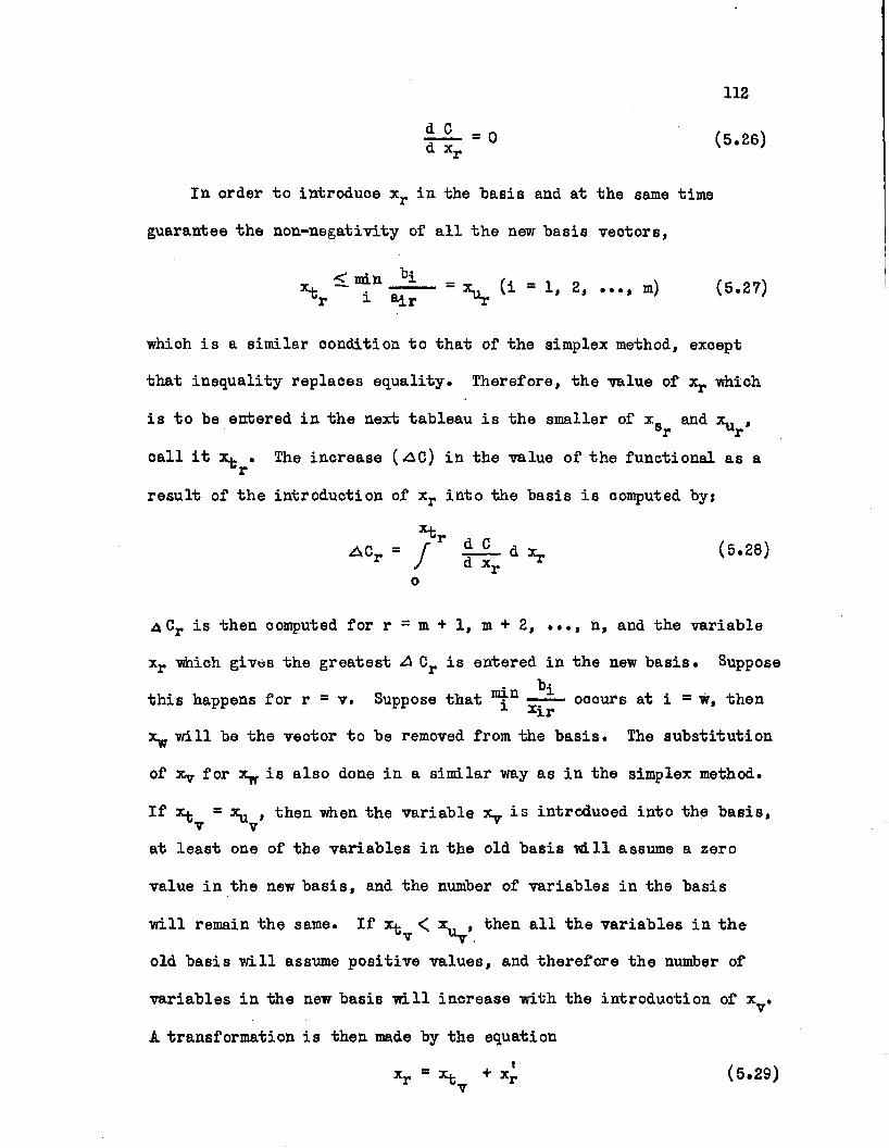
In order to introduce xy in the basis and at the same time

guarantee the non-negativity of all the new basis vectors,

^ I57-- 2i - . m ) (5.27)

which is a similar oondition to that of the simplex method, except

that inequality replaces equality. Therefore, the value of Xj. which

is to be entered in the next tableau is the smaller of x_ and x., ,r ur

call it ^ . The increase (^C) in the value of the functional as a

result of the introduction of xr into the basis is computed by*

■ T " r i 4 * C6-29)O

A C r is then computed for r = m + 1, m + 2, ..., n, and the variable

xr which gives the greatest A Cr is entered in the new basis. Suppose1711 71 ^ithis happens for r = v. Suppose that ^ — — occurs at i = w, then

x . will be the vector to be removed from the basis. The substitution

of Xy for x . is also done in a similar way as in the simplex method.

If X. = xl, , then vixen the variable x . is introduced into the basis, v v

at least one of the variables in the old basis will assume a zero

value in the new basis, and the number of variables in the basis

will remain the same. If n. < x,, , then all the variables in thev uv .old basis will assume positive values, and therefore the number of

variables in the new basis will increase with the introduction of x .vA transformation is then made by the equation

113

where x . is a new variable. The original m equations are modified by-

substituting the transformation in each of the original m equations

in order to eliminate Xp and to introduce x^. The new set of (m+l)

equations consist of equation (5.29) and the m equations in which

Xp is substituted for xr« The method of continuing the calculations

after this transformation is similar to the calculations previously

described. Generally, each tableau is checked for optimality until

one is reached, in which no increase in C is possible with the intro­

duction of a new variable.

Nonlinear Programming

Kuhn and Tucker^- treated the general case when both the constraint

conditions and the oriterion function are nonlinear. The original

linear programming problem of maximizing a linear function C (x) = nZ o. x. where j =1, 2, 3, ..., n, (i.e. x is an n-component vector)j=l 3 3under the conditions that:

nfi (x) = b.-I' xj> 0 (5.30)

x j > 0 (5.31)

where i = 1, 2, ...., m, is transformed into an equivalent problem.

Suppose the Lagrangian function (x, u), is formed such that,m

$ (x, u) = C (x) + 2: u^ (x) (5.32)i=l

i.e.m n

$ (x, u) = C (x) + 21 u± ( ^ - Z. a., x.) (5.33)i=l j=l 3 3

TI Kuhn, H. Iff., and Tucker, A. W., ’Nonlinear Programming." Jerzy Neyman, Second Berkeley Symposium on Mathematical Statisties and Programming, (Berkeley: University of California, 1951).

114

orn m m n

^ U. u) = Z ei*i + £ biui “ £ Z aii m i, (5.34)j=l i=l i=l j=l J J

A saddle value or miniraax problem which is equivalent to the maximi­

zation problem is that of finding some vector u° with non-negative

components such that:

0 (x, u°)< $ (x°, u°)<: $ (x°, u) (5.35)

A particular vector x° which satisfies the constraints (5.30) and

(5.31) will maximize C(x) if and only if a veotor u° satisfying

(5.35) exists. Such a statement of the problem oontains its dual.m

The dual problem is that of minimizing B (u) = 27 bi ^ 2,...,m)i=l

subject to the conditions that

mgj(u) = 0 ^ - 2 7 a^j ut < 0 (5.36)

and Uj > 0 (5.37)

j — 1. 2, ...> n

The solution of both the original problem and its dual are contained

in the saddle point (x°, u°) satisfying (5.34) and (5.35). The

minimum maximum roles of u and x can be interchanged by replacing

4 (x) by (x). It should be noted that the saddle point (x°, u°)

provides a solution to a related zero-sum two person game. The

veotor x° represents the strategy of the maximizing player, and u°

represents that of the minimizing player.

This treatment of the problem oan be extended even when neither

C(x) nor f^(x) are linear. Kuhn and Tucker found the neoessary and

sufficient conditions for a saddle value for any differentiable

function $ (x, u), and applied them to find the maximum of a differen­

116

tiable function C(x), under inequality constraints described by

differentiable functions f- (x). The necessary conditions for a

saddle point are derived from the known requirement of zero value for

the derivative of a function at its maximum or minimum. Thus the

partial derivative of $ (x, u) with respect to all the components

of x and u should vanish at the point (x°, u°)» except possibly when

the corresponding components of x°, u° are equal to zero.

The equivalence of the saddle value problem and the maximization

problem was established by Kuhn and Tucker when the functions fi(x)

are oonoave as well as differentiable for x > , 0 .

CHAPTER VI

ATTEMPTS FOR SIMPLIFIED METHODS

The review presented in the last chapters shows that existing

methods for solving the linear programming problem, especially in

the general case, require lengthy computations when the number of

variables or the number of restrictions is above average. For many

cases, the linear programming model does not describe an unchanging

situation. The variables, their relationships*and the price attached

to them often change in such a way as to require new computations.

Sometimes, it is only necessary to use the data in the final tableau

to calculate the effect of changes in the original data; for example,

when one of the variables appearing in the final basis is restricted

to a value lower than the value it assumes. In this case, the final

tableau tells us which of the nonbasic variables causes the least loss

by its introduction into the basis. It is the variable with minimum

non-negative 2^-c^ (there are no negative zj”cj the final tableau).

This is an example where few additional calculations are needed.

Usually, a restatement of the problem is needed. TOien these variations

are frequent enough, and with a medium size linear programming problem,

computations may be too costly and time-consuming. It will not be

worthwhile putting a great effort in calculating a program which will

be carried out only for a short period. Therefore, the need for

quick, and maybe approximate, methods of solving the linear programming

problem arose*

116

117

As a participation in the effort to devise easier computing

procedures, the author made some attempts, -which will be presented

in this ohapter.

THE ENVELOP METHOD

The first attempt can be better illustrated with reference to

the two-dimensional case. Consider the set of inequalities:

ail X 1 + ai2 x2 ^ bi (6.1)

where i “ 1, 2,..., m. Take i = 3.

Maximize C = oj + Og Xg subject to (6.1) and

*!■ *2 > 0 ( 6 . 2 ).

Figure 4

In Figure 4 the set of inequalities are represented by an area

bound by the straight lines, 1, 2 and 3, representing the inequalities,

and the axes x^ = 0 and xg =0. The criterion functional would be

118

represented by a set of parallel straight lines each of which corres­

ponds to a particular value of the functional. The idea, in the new

attempt is to replace the original set of points S defined by inequa­

lities (6.1) and (6.2) by a set S1 such that each point in the new

set satisfies (6.2) and

xx < x [ and x2 < x^

where

x-, s inf x^ and Xg 2 inf x^S xgtS

(inf means the least upper bound)

The optimum point is to be obtained for S* instead of S. The broken

lines in Figure 4 represent two values of the criterion function,

then point A is the optimum point for the original set, and point B

is the optimum point for the new set. It is easier to find the opti­

mum point for the new set, especially when the simplex method is

used, since a smaller number of extreme points will be explored.

However, the author found no reasonably easy method for determining

the values of x^ and Xg. The knowledge of these two values implies

the knowledge of an extreme point maximizing the criterion function

C = xj and C = Xg, which is obtained only by the solution of the problem

with these two functionals as successive criteria.

A SPECIAL CASE OF THE CRITERION FUNCTION

Consider the set of inequalitiest

na^j XjjCb^ (6.3)

119

■where j = 1, 2,....,nj and i = 1, 2,..., m.

A linear programming problem would be to maximize a linear functionaln

C o-? x-? (6*4)3=1 5

subject to (6.3) and

X j O 0 (6.5)

Suppose that instead of C in (6.4) we have a functional

C* = xk where xk can be any of the xj's. Therefore, the maximum value

of the functional can be obtained as follows. Put xk equal to the

maximum value that it can assume in each one of the equations. 'When

the coefficients a ^ in the inequality i are preceded only by plus

signs, then the greatest value that xk can assume in this inequalityh. /is i , putting the coefficients of x. for j f k equal to zero.

aik J

[ H i X1 + H .2 x2 + + aik xk +*’* + ain xn — **i *for max-, xk , put a ^ = 0 for j £ k,

,\ a jj. Xjj. <; b^

Again, to maximuze xk let aik x^ = b^ where (x^)^ is the maximum xkb*for restriction i; i.e. max (x,) = _L_ (6.6)"]

1 H ) J

The maximum value that x^ can assume in the set of inequalities in the

minimum of the maximum xk in all the inequalities.

max xk = nnn max (x^), (6.7)

Putting x^ equal to this value and solving the set of linear

inequalities for the rest of the variables may give us a solution to

the linear programming problem presented above. The word ’'may" is

inserted to indicate that sometimes this is not the solution. The

reason is that the Xj*s thus obtained may have negative values, and

120

hence restriction (6.5) m i l not be satisfied, or else imposing these

restrictions will yield no solution for that particular value of x^.

A refinement of this method is presented in the next chapter.

A STUDY IN THREE DIMENSIONS

This attempt takes advantage of the easier form of a oriterion

funotion with one variable. If the functional is originally in the

formn

0 = £0=1 J

then it oan be converted to a Bingle variable by adding the restriction

xn+l = °1 X 1 + °2 x2 + •••• + cn xn (6*8)The criterion then can be; maximize xn+q*

Consider the set of two equations;

a ll X1 + a12 x2 + a13 x3 = bl (6*9

a21 X 1 + a22 x2 + a23 x3 = b2

and suppose that it is required to maximize Xg, subject to (6.9) and

xli x2t x3 > 0 (6.10)

The two equations represent two planes in a 3-dimensional space,

whose coordinates are x^, xg, xg. There are three possibilities;

1. The two planes will not intersect; i.e. the two equations are

inconsistent. In this case there is no solution for the set of two

equations.

2. The two planes will intersect in a straight line which falls

completely in the negative half-space, in which case there are solu­

tions to the set of equations (6.9), none of which satisfy the

non-negativity restriction (6 .10).

3. The two planes will intersect in a straight line, a part of

which lies in the positive half-space. There are two possibilities

here.

a. Only one point of the line is non-negative. This will

be the solution to the linear programming problem.

b. A set of more than one point is non-negative. Then, it

is required to find that point in the set, which has the maximum

coordinate xg.

Figure 5

A suggested procedure to find this point ist

1. Find the maximum value that Xg can assume in each one of the

two equations. These will bet, . bn

122The minimum of these two values cannot be exceeded by the optimum

value of X3, which satisfies restrictions (6.9) and (6.10). (This

value will be called Xg.)

Xg = mrix. Xg ~ min (xg) i=l,2 1

If X3 in the equations (6.9) is given the value (xg), then x- and xg

can be determined. The point specified by the coordinates x^, Xg and

Xg thus obtained may have all non-negative coordinates, and in this case

it will be the solution, or else some of its coordinates will be negative.

The first case is represented by point A in Figure 5A. In the second

case, we distinguish three points*

A. The optimum point (x°, x°, x°), that is the point on the line1 c» oof intersection of the two planes which has the maximum Xg. This is

represented by point A in Figure 5B. Since we only have two equations,

then no more than two of these coordinates will be nonzero. Therefore

either x° or x° will be equal to zero. Also, from Figure 5B, it can

be easily seen that A lies on the border between the positive and the

negative half-spaces, therefore either x° or x° will vanish. It can

also be noticed that if we go along the line of intersection of the

two planes in the direction that increases Xg we will be in the negative

half-space, such that the negative coordinate will be the one which was

originally null.

,B. The point (0, 0, Xg).

C. The point (xp xg, x^), which is given by substituting Xg in1 »

equations (6.9) and solving for x- , xg.

The last two points are represented by points B and C in Figure 5B.

Since Xg is at least equal to Xg, then;

a. If neither x^ nor Xg is negative, xg = xg and the pro­

blem reduces to that of Figure 2A.

bi If either x^ or Xg (or both) is negative, then x^ ;> x°.

In this case, the negative coordinate is the one which was originally

zero at the optimum point. Putting that coordinate equal to zero in

equations (6.9), and solving for the other two variables, the optimum

solution is obtained.

This is obviously a valid method of solution in the three dimen­

sional case. "When more dimensions are present in the problem, addi­

tional difficulties are faced. These can be illustrated by the four­

dimensional case.

Consider the two equations;

all *1 + a12 x2 + al3 X3 + *14 X4 " bl(6.11)

a21 X1 + a22 x2 + a23 x3 + *24 X4 = b2

It is required to maximize x4 subject to the restrictions (6.11) and

xl* x2* x3* x4 (6.12)Each one of the two equations represents a 3-dimensional hyperplane

in a 4-dimensional space, which intersect in a plane. Consider only

the case when the two hyperplanes intersect in a plane a part of whichI

is in the positive half-space. Suppose that x^ is obtained in the same

way as x* in the last problem, i.e. o

124

Substituting x^ for x^ in the two equations (6.11) and solving

them for x- , Xg, Xg, after assigning a zero value arbitrarily, the

outcome will be one of two casesj

a. All coordinates x^, Xg, X g are non-negative, in which case

x4 = x4 anti 'tiie optimum solution is achieved

b. Some x^, x.% or xg is negative.

Consider now the 3-dimensional space formed by the intersection

of the three-dimensional hyperplane x^ = and the 4-dimensional

spaoe considered above. The intersection of the hyperplane x^ * x^

with each one of the equations (6.11) will be a 2-dimensional plane.

These two planes will intersect in a straight line (call it S). If ai it

part of this straight line is in the positive half-space, then xA = x^,

and the optimum point (or points) is reaohed. By assigning an arbitrary

value of zero to one of the variables we try to detect the location

of the point of intersection of the straight line S, and one of the

planes of intersection of the 3-dimensional hyperplanes x- = Xg = Xg = 0,t

with the hyperplane x^ = x^. If all these three points are in the

negative half-space, then no part of the straight line contains the

optimum point (or points), and x^>x£. As x^ is reduced, other

straight lines S, parallel to the first, will be obtained, each one

having three points which represent the intersection of the straight

line with the planes of intersection of each of x- = 0, Xg = 0 and]|( jjt

Xg = 0 with the hyperplane x^ t= x^, where x^ is the value given to x^%such that x^< x^. If the set of all possible lines S is drawn,

they will fall in a plane with straight lines (L) representing the locii

of the points of intersection mentioned above (Figure 6}) • Since there

125are two restricting equations, at most two of the variables will be

nonzero at the optimum point, that is at least two of them will be zero.

Figure 5

Therefore the optimum point oan only be one of the points A, B or C.

Since C (the intersection of anc* x3=®) ^as a negative coordinate

(x^), then the optimum point is either A or B. Whether A or B is the

required point is determined by the orientation of the set of lines S

and the direction of their movement when x^ is decreased. Suppose

that S]_ is one of these straight lines, and that its movement for

decreasing x^ is indicated by the arrow, then for maximum x^, the

optimum point should be A* The same argument used in the 3-dimensional

oase can be applied here and one oan say that the first point in the

positive space that meets the moving line S is the optimum point.

However, no reasonable method could be found to find this point by

detecting the positive and negative coordinates of the points of inter­

section of the line S with the set of lines L.

CHAPTER VII

NEW APPROACHES

THE ELIMINATION METHOD

Consider the system of inequalities in the unknowns x.,J

nZ- (7.1)3=1 J J

where i = 1, 2, m.

and j = 1, 2, ...,n.

One method of finding a solution is by eliminating the variables

successively. To eliminate its coefficient a ^ in each of the

inequalities is examined and,

if &ijc> 0, the inequality i is classified under type A

if a fc < 0, the inequality i is classified under type B

if a ^ = 0, the inequality i is classified under type C

To eliminate x^, eaoh inequality of type A is added to each one

of type B, after multiplying with necessary factors. The new system

together with inequalities C will be void of the variable x^.

The elimination method as such is already known. However, it is

adapted in this section to solve the linear programming problems.

Consider the linear programming problemi

nMaximize C = £! Oi x. (j = 1, 2, .»», n) subject to (7.1) and

j=l J J

xj > 0 (7.2)

126

127

The general outline of the procedure to solve this problem by the

elimination method is:n

1. Put xa+1 * <T cj xj (7.2)

2. Eliminate as many as possible of the variables xj except

xn+l* left is a system of inequalities containing xn+]_

only or xn+ plus one or more variables such that the coefficients of

each variable will have the same sign in all the inequalities.

3. The three possible cases are;

a. xn+i exists alone. The procedure will then oonsist of

determining both the least upper bound of (Sup from the

last system of inequalities and assigning this value to xn+ .

b. xQ+1 exists together with a group of variables all having

positive coefficients. In this case Sup xn+ is obtained by setting

all the other variables equal to zero and proceeding as before.

c. Other variables exist with xa+]_, the coefficients of

some of which are negative. The least upper bound of xn+^ in this

case will be infinity.

4. After finding in this way, the variable that was

eliminated last could be obtained by substituting the value of xn+ ,

and the variables that are equated to zero, in the previous Bystem of

inequalities. Proceeding in this manner, all the other variables

can be obtained.

5. It should be noticed that the set of inequalities (7.2), i.e.

the set of non-negativity restrictions, was not explicitly considered

120

in the last procedure. For this reason one may find some negative

variables in the solution. As soon as the value of any variable is

found to be negative, the variable eliminated directly after it,

i.e. the variable evaluated directly before it, is examined to see

whether any increase in the value of the negative variable is possible

by a change in its value. If an elimination of the negativity of that

variable is not possible with a change in this variable, the one

eliminated after it is tried and so on until the variable satisfies

(7.2). A reduction of xn+]_ might be necessary for this purpose.

As an example for this method of solution the linear programming

problem presented in Charnes^, and which is solved by the simplex

method is presented here.

The numbers of the equations in this example will be preceded

by E to distinguish them from the other equations in the rest of the

chapter. The problem is to maximize

C = -15 xi + 25 xg + 15 X3 - 30 x^ + 10 Xg + 0 Xq -40 Xy - 10 Xg

subject to inequalities (E 1-7) and to the non-negativity restrictions. .

Dividing C by 10, an equation (E 8) is formed by introducing x ^ q = c / l O .

1. Charnes, A., Cooper, W.W. and Henderson A. An Introduction to linear Programming. (New York* Wiley, 1953).

X]£ + 1.5 x- - 2.5 Xg

To eliminate x^t

Prom

(E 1) and (E 5)

(E 2) and (E l)

(E 1) and (E 8)

(E 2) and (E 8)

To eliminate xgj

From

(E 3) and (E 4)

(E 4) and (E 7)

129

-xx + x2 + x3 < 0 (El)

-xx + 3x2 - x5 < 0 (E 2)

-3 x 4 + x5 + x6^ 0 (E 3)

"x4 + x5 " x6 - 0 (E 4)

x1 + x4 + x7 < 100 (E 5)

x2 + xg + Xg 100 (E 6)

Xg + Xg + xg 5 60 (E 7)

1.5 Xg + 3 X^ - Xg + 4 Xy + Xg = 0 (E 8)

x2 + x4 + x3 + x7 - 100 9)

3 X2 + x4 — Xg + Xy 100 ( E 10)

-Xg + 3 X4 - Xg + 4 Xy + Xg + X^q £ 0 (E ll)

2 Xg - 3 Xg + 3 X4 - Xg + 4 Xy + Xg + X^q40

(E 12)

-2 x4 + X g 1 0 (E 13)

X3 " X4 + X5 + X9 “ 60 14)

130

To eliminate x^t

Prom

(E 9) and (E 15)

(E 10) and (E 13)

(E 11) and (E 13)

(E 12) and (E 13)

(E 9) and (E 14)

(E 10) and (E 14)

(E 11) and (E 14)

(E 12) and (E 14)

To eliminate xg:

From

(E 15) and (E 16)

(E 19) and (E 16)

(E 21) and (E 16)

(E 15) and (E 18)

(E 19) and (E 18)

(E 21) and (E18)

2 Xg + 2 Xg + Xg + 2 x7 — 200 (E 15)

6 X2 - 2 xg + Xg + 2 X7 200 (E 16)

-2 x2 + xg + 8 xy + 2 Xg + 2 *10^ 0 (E 17)

4 x2 - 6 x5 + Xg + 8 x7 + 2 Xg + 2 x1Q ^ 0 (E 18)

x + 2 x + x + x + x 160 ^ ^

3 Xg + Xg + x7 + Xg < 160 (E 20)

- Xg + 3 Xg + 2 Xg + 4 x7 + 4 Xg + x^0 180 (E 21)

2 Xg + 2 Xg + 4 x 7 + 4 Xg + x1Q 180 (E 22)

4 xg + xg + 2 i ? < 200 (E 23)

7 Xg + 2 Xg + 3 x 7 + Xg ^ 3 6 0 (E 24)

16 xg + 7 Xg + 14 x 7 + 8 X 9 + 2 Xjy£960 (E 25)

5 Xg + 2 Xg + 7 x 7 + xg + x^Q — 300 (E 26)

7 Xg + 4 Xg + 11 x 7 + 3 Xg + 2 x-jq 480 (E 27)

2 Xg + 3 Xg + 16 x 7 + 10 Xg + 4 Xjg ^ 3 6 0 (E 28)

131To eliminate Xg;

From

E 6) smd (E 17) 3 Xg + 8 Xy + 2 Xg + 2 Xg + 2 X ^g £. 200 (E 29)

E 20) and (E17) 5 Xg + 26 x? + 8 xg + 6 *1 0 - 320 (E 30)

E 22) and (E 17) x5 + 4 X y + 2 Xg + X^g < 60 (E 31)

E 23) and (E 17) 3 Xg + 18 Xy + 4 Xg + 4 x10 £ 200 (E 32)

E 24) and (E 17) 11 Xg + 62 X y + 16 Xg + 14 x10 £720 (E 33)

E 25) and (E 17) 15 Xg + 78 X y + 24 Xg + 18 x1Q £ 960 (E 34)

E 26) and (E 17) 9 Xg + 54 X y + 12 Xg 12 x10 £600 (E 35)

E 27) and (E 17) 15 Xg + 78 X y + 21 Xg + 18 x1Q £ 960 (E 36)

E 28) and (E 17) 2 Xg + 12 Xy + 6 Xg + 3 X10 - 180 (E 37)

The restrictions on the values of x- g are imposed by inequalities

(E 29) to (E 37)* No further eliminations can be made "with this system

of inequalities. To maximize x^g the other variables should be equated

to zero (since they are all preoeded by plus signs). Therefore,

x5 = x7 = x8 = x9 = 0 (E 38)

The least upper bound of x^g =5 0 (E 39)

■which is imposed by inequalities (E 32, 35).

The restrictions on xg are given by (E 6, 17, 20, 22 - 28). Sub­

stituting for the values of X g , X y , X g , X g , x ^ g ,

Sup Xg = 50

as given by inequalities (E 23, 26) and

Inf X2 - 50

132as given by (E 17)

x2 = 50 (E 40)

X3 is restricted by (E 15, 16, 18, 19, 21)#

(E 15) dete rmines Sup xg = 50

and (E 16, 18) determine Inf xg = 50

••• Xg = 50 (E 41)

x^ is restricted by (E 9 - 14)

Sup = Inf x4 = 0

x4 = 0 (e 42)

xg is given by (E 3, 4, 7)

x6 = 0 (E 43)

x-l is given by (E 1, 2, 5, 8)

From (E 1, 2) x- 100

From (E 5) x^ 100

From (E 8) x^ = 100

= 100 (E 44)

The final solution is then:

x-j_ = 100 Xg =50 Xg = 50 x^o = 50

which coincides with the solution by the simplex method.

The main drawback in this approach is that the number of equations

is liable to increase, as has been demonstrated in some of the steps

of the last example. The greatest increase occurs when the equalities

are equally distributed between types A and B.

This method is particularly economical when the number of variables

is large but the number of equations is small, or when the number of

equations is large but each variable appears in a small number of

equations.

In this last example, the number of steps is 44 less the original

7 equations, that is 37. In the simplex method six tableaus were needed,

each consisting of 8 lines, with a total of 48 steps.

A procedure which may be expedient in carrying out the computations

according to the elimination method, when the variables are determined

by range of values rather than by single values, isj

1. Lower and upper bounds are established for the variable

eliminated last.

2. Lower and upper bounds for the variable eliminated directly

before it are obtained based on the lower and upper bounds of the last

one.

3. Proceed in the same manner for the rest of the variables.

4. If any of the variables has a negative lower bound the upper

or lower limit of the variable eliminated directly after it is checked

to see whether any increase in the value of the negative variable is

possible through changing this limit. If the negativity of that vari­

able is not eliminated, proceed to the variable eliminated directly after

the last one, and so on until the lower bound of the variable in question

Is non-negative. This may not be aohieved except after a reduction in

the value of the variable xn+i«

It should be noted that an alternative to this procedure is to take

the nonnegativity restrictions into consideration from the beginning.

Therefore, if x^ is the variable in question, the inequality

134

would be combined with each one of the equations of type B (if any exists)

whose form would be:

to give an inequality of the form

Z H j > o J-l

which would be treated with the rest of inequalities. According to this

procedure, the value of the least upper bound of xn+ (the variable to

be maximized) obtained after eliminating the rest of the variables, would

be its optimum value.

THE TRANSFORMATION METHOD

As has been pointed out earlier in this study^, the linear programming

problem:n

Maximize C(x) = 21 c. x.j=l J J

where j = 1, 2, ...., n, under the condition that:n

fi (x) - b^ - 21 a. . x. >. 0 .1=1 1J J

(7.3)

x.> 0J (•7.4)

where i = 1, 2, ..., m, can be transformed into another problem by forming

the function $ (x, u) such that:

1. Supra p. 114.

■where

Uj > 0 (7.7)A solution to the original problem can be obtained if and only if a

point (x°, u°) is found such that:

4 (x, u°) <r4 (x°, u°) < 4 (x°, u) (7.8)

for all x, u. In the discussion that follows we assume the problem is

such that the vectors u° and x° exist.

Suppose a rotational transformation could be made to a new set of

coordinates r, s such that:

U i u) = (r, s) = (r) + ©2 (s) (7.9)

That is the new function is a separable function in r and s. it is

then required to find the point (r°, s°) such that:

(r°,s)< f (r°, s°) ^ (r, s°) (7.10)

where r, s, are vectors

i.e.

»1 (r°) + © 2 (s)^ Q 1 (r°) + ©g (s°) (r) + ©2 (s°) (7.11)

A consequence of (7.9) is that there is a value r° of r that will minimize

9 (rj) independently of the value of s, i.e. there exists an r° such that

for each r:

nani °1 = ®1 (r° ) ^ ©i (r) (7.12)

136

If this were not true, then there exists an r such that

©x (r) > (r°) (7.13)

Therefore,

©! (r) + ©2 ^ > ®1 (l*0) + ®2 (s°) (7.14)

contradictory the assumption that u° and x° exist which satisfy (7.11).

Similarly there exists an s° such that for each s

©2 (s) 5 ©g (s°)^-®2

8°) = T ®]_ (r) + T 0 z (b)

(7.15)

(7.16)

Therefore to reach the saddle point one has pnly to minimize ©^ (r)

relaxation procedure that the author suggests to obtain the saddle point

in terms of r and s, which can be translated in terms of u and x. If a

transformation is found which will satisfy (7.9), and if a procedure is

obtained according to which ©^ (r) is minimized, or decreased in each

successive approximation, then one will converge to the saddle point.

Following is an example of the application of this principle in the case

of one-dimensional vectors (scalars) r,s.

Example:

Maximize x under the conditions that

irrespective of s and then maximize ©2 (s) irrespective of u, or proceed

by decreasing ©]_ (r) and increasing 0£ (s) successively, and this is the

iterative step, and ©2 (s) is maximized, or increased in each step of

x < 1

and

x > 0

157

The problem be replaced with the problem;

Find (u°, x°) such that

$ (u, x0) ^ ^ (u°,x°) ^ <ji (u°, x)

and

u 0

where

$ (u, x) = x + u (1 - x)

= x + u - ux

The surface produced by this equation is a saddle surface whose

intersection with planes parallel to the (x - $) plane or to the

(u - $) plane produces sloping straight lines; its intersection with

planes parallel to the (x - u) plane (i.e. for different values of

produces hyperbolas whose asymptotes are the lines x = 1 and u = 1.

The saddle point occurs at a value of $ (x, u) for which the hyperbola

becomes the two above mentioned asymptotic lines. The saddle point is

the intersection of these two lines, namely the point x = 1, u = 1.

To obtain that analytically;

Put x = “ 7 (r - s)) T

and u = — - (r + s)fT

4 (x> u) = "ZT (r + s) + “TT"- (r - s) - w (r s )[ 2 f z .

= / T r - I r2 + | s 2 (r, s)

f (r, s) = (r) + ©2 (s)

138

This linear transformation is equivalent to rotating the axes such

that the r-axis passes through the vertices of the hyperbola, that is

the (r - $ ) plane forms one of the axes of the saddle surface. The

s-axis is perpendicular to the r-axis. The intersection of the pianos

s = constant with the saddle surface forms parabolas whose slopes are

independent of s

“ x 81 (r) - ( ( 2 r - 1 r2)

' ®1 , ,-------— —- = / 2 - r = 0 , therefore r = tT2

^ 9 2 = s = 0 , therefore s = 0H s

From which

x = 1, and u = 1

When x and u are vectors having more than one dimension, then the

transformation of the function

n m$ (x, u) = z : c. x. + 2 T b. u. - £ 2 a. . u. x. (7,17)

j=l 3 3 i=l f j j 3 3

t \ 1into a separable function of two variables (r, s) runs as follows:

Suppose that m ^ n

Let y^ = 2T xj i = 1, mj

ym+o< = xm + c< «* = 1, ..., n-m

1. The transformation presented here was suggested by Dr. D. R, Whitney.

139If the determinant Isijl / 0,

and if matrix (A~^) is the inverse of matrix (A) = (a. .)

(xj) = (A-1) (35)

m m mf (y, u) - £ Cj yj + ^ bj Uj - ^ Ui yi

i=l < = 1 i=l

Let ui = Ti + Si i = 1, ..., m

yi = ri " si

ym+ *" r m+<* o< - 1, ..., n-m.

„ ® n m m4 (r,s) = Z c- (ri“3i) 4 ^ °i i*i + Z. b. (ri+si) + Z (rf-sf)

i=l i=m+l i=l i=l

i.e. 5/" (r,s) = ©1 (r) + 9£ (s)

If m > n, the u and x would be exchanged in the previous procedure.

Once the function is transformed into this form, 9^ (r) and 9o (s)

could be maximized or minimized separately. Since 9- (or 92) is a

function of a vector, it may be possible, through the application of an

appropriate relaxation decision criterion, to start with any point,

and relax one of its dimensions such that the value of 9i (or 90) U

increases (or decreases). Another dimension could then be relaxed and

so on until the maximum (or minimum) value of the function is reached.

140BIBLIOGRAPHY

1. Agmon, Shmuel, "The Relaxation Method for Linear Inequalities.", National Bureau of Standards. National Applied Mathematics Laboratory Report, Vol. -52-57, 1952.

2. Bellman, Richard, "Some Problems in the Theory of Dynamic Programming."Econometrioa, Vol. 22, No. 1, January 1954, pp. 46-47.

3. Bellman, R., Glicksberg,I., and Gross, 0., "On Some VariationalProblems Occurring in the Theory of Dynamic Programming."National Academy of Sciences Proceedings, Vol. 39, No. 2, Feb.,1953, pp. 298-301.

4. Bross, I. D., Design for Decision. New York, The McMillan Co., 1953.

5. Charnes, A., and Cooper, W. W., "The Stepping Stone Method ofExplaining Linear Programming Problems." Management Science Vol. 1, No. 1, Oct. 1954, pp. 49-69.

6. Charnes, A., Cooper, W. W. and Henderson, A., An Introduction toLinear Programming, "Wiley, New York, 1954.

7. Charnes, A», Cooper, W. VL, and Mellon, B., "Blending AviationGasolines," Econometrioa, April, 1954.

8 . Dantzig, G. B., "Linear Programming Under Uncertainty." ManagementScience, Vol.l, No. 3-4, April-July 1955.

9. , "Status of Solution of Large Scale Linear ProgrammingProblems,'1 Road Corporation Research Memorandum RM-1375 U.S.A.F. Project, 9 pp.

10. , "Upper Bounds, Secondary Constraints and BlockTriangularity in Linear Programming," Econometrioa, Vol. 23, No. 2, pp. 174-83, April, 1955.

11. Pantzig, G., Fylkerson, R., and Johnson, S., "Solution of a LargeScale Traveling-Salesman Problem", _J. Operations Research Society of America, Vol. 2, No. 4, Nov. 1954, pp. 393-410.

12. Flood, Merril M., "The Traveling-Salesman Problem," _J. of OperationsResearch Society of America, Vol. 4, No. 1, Feb. 1956.

13. Ford, L. R., and Fulkerson, D. R», "Maximal Flow Through a Network."Notes on Linear Programming; Part XX, U.S.A.F. Project. RandCorp. Research Memorandum RM-1400, Nov. 1954, p. 2.

14. Gaddum, J. "W., Hoffman, A. J., and Sokolowsky, D., "On the Solutionof the Caterer Problem," Naval Research Logistics Quarterly,Vol. 1, No. 3, Sept. 1954, pp. 223-232.

141

15. Heller, Isider, "On the Problem of Shortest Path Between Points -Parts I, II," American Mathematical Sooiety Bulletin, V. 59, 1953, pp. 551-2.

16. Henderson, A., and ScHaiTer, "Mathematical Programming. BetterInformation for Better Decision Making." Harvard Business Review, Vol. 32, No. 3, May-June, 1954.

17. Houthaker, H. S. "On the Numerical Solution of the TransportationProblem," J. Operations Research Society of America, Vol. 3,No. 2, May, 1955, pp. 210-214.

18. Jacobs, Walter, "The Caterer Problem," Naval Research LogisticsQuarterly, Vol. 1, No. 2, June 1954, p. 155.

19. Koopmans, Trailing C., Activity Analysis of Production and Allocation.Cowles Commission, Wiley, New York, 1951'. "

20. Kuhn, H. W., "The Hungarian Method for the Assignment Problem,"Naval Research Quarterly, V. 2, Nos. 1, 2, March-June 1955, pp.83-98.

21. Kuhn, H. W., and Tucker, A. W., "Nonlinear Programming." JerzyNeyman, Second Berkeley Symposium on Mathematical Statistics and Programming. (Berkeley; University of California, 1951).

22. Morton, 6., "Notes on Linear Programming." Economica, XVIII, 72,November 1951.

23. Pepper* P. M. and Mitten, L- G., Balanced Scheduling of ProductionFacilities (mim.), The Ohio State University, 1955.

24. Russel, Bertrand, The Scientific Outlook, Glencoe, Illinois, FreePress, 1931.

25. Saline, L. E., "Quadratic Programming of Interdependent Activitiesfor Optimum Performance," The American Society of Mechanical Engineers Paper No. 54-A-58, 1954.

26. Salveson, M. E., "On a Quantitative Method in Production Planningand Scheduling." Eoonometrioa, Vol. 22, No. 1, October, 1952.

27. Symposium on Linear Inequalities and Programming, U.S.A.F. ProjectSCOOP No. 10.

28. Symonds, Gifford H., Linear Programmings The Solution of RefineryProblems, Esso Standard Oil Company, New York, 1955.

29. Temple, G., "The General Theory of Relaxation Methods Applied tolinear Systems." Proceeding of the Royal Society of London,Series A, Vol. 169, 1939, pp. 476-500.

142

30. Taylor, F. Yf., Scientific Management. New York, Harper and Brothers,1947.

31. Von Neumann, John, "A Model of General Economic Equilibrium,”The Review of Economic Studies, Vol. XIII, 1945-46.

32. Yfilkinson, J. J., "Better Management = Management + IndustrialEngineering + Linear Programming," J. of Industrial Engineering, Vol. VII No. 1, Jan-Feb. 1956, pp. 11-23.

AUTOBIOGRAPHY

I, Mohamed Ibrahim Dessouky, was born in Cairo, Egypt, in 1926,

and received my elementary and secondary education there. I obtained a

Bachelor of Science in Mechanical Engineering at Cairo University in

1948. After working in the Coca-Cola Bottling Company in Cairo for less

than a year, as an Assistant Plant Superintendent, I transferred to the

Egyptian State Railways and worked as a Tooling Engineer for a period of

two years. In 1951, I joined the staff of Cairo University as an

instructor ("demonstrator”) in the Department of Mechanical Engineering.

In September of 1953, I attended Purdue University, receiving an M. S.

in Industrial Engineering in August 1954. I then continued my studies

at The Ohio State University in Industrial Engineering, and was awarded

a Ph. D. in December 1955.

143