Behavior appraisal of steel semi-rigid joints using Linear Genetic Programming

Journal of Constructional Steel Research 65 (2009) 1738–1750

Contents lists available at ScienceDirect

Journal of Constructional Steel Research

journal homepage: www.elsevier.com/locate/jcsr

Behavior appraisal of steel semi-rigid joints using Linear Genetic ProgrammingA.H. Gandomi b, A.H. Alavi c, S. Kazemi a, M.M. Alinia a,∗a Department of Civil Engineering, Amirkabir University of Technology, Tehran, Iranb Tafresh University, Tafresh, Iranc Iran University of Science & Technology, Tehran, Iran

a r t i c l e i n f o

Article history:Received 25 September 2008Accepted 12 April 2009

Keywords:Semi-rigid jointsSteel structuresLinear genetic programming

a b s t r a c t

This paper proposes an alternative approach for predicting the flexural resistance and initial rotationalstiffness of semi-rigid joints in steel structures using Linear Genetic Programming (LGP). Three typesof steel beam-column joints i.e. endplates, welded, and end bolted joints with angles are investigated.Models are constructed by utilizing test results available in the literature. The accuracy of the proposedmodels is verified by comparing the outcomes to the experimental results. LGP models are furthercompared to the corresponding design code (Eurocode 3), reference values and several existing models.The results demonstrate that the LGP based models in most cases provide superior performance thanother models.

© 2009 Elsevier Ltd. All rights reserved.

1. Introduction

Steel framemulti-story structures have threemain componentsnamely, beam, columns and joints. In reality all joints are semi-rigid, but formal codes acknowledged them as either pinned orrigid; having their own advantage and disadvantages. Althoughthese simplifications ease structural analysis and design, they donot reflect the actual behavior of beam-column joints.Modern standards, such as Eurocode 3, classify joints according

to their actual behavior. Thus, according to their rotationalstiffness, theymay be classified as nominally pinned, rigid or semi-rigid [1]. This is carried out by comparing their initial rotationalstiffness (Sj,ini) with the classified boundaries illustrated in Fig. 1.According to Eurocode 3, all beam-column joints in zone 2 ofFig. 1 should be classified as semi- rigid and other joints in zones1 and 3 may also optionally be treated as semi-rigid. The twomain structural characteristics in joint design are their flexuralresistance and initial rotational stiffness. Eurocode 3 providessome formulas and tables for computing these properties whichdepend on many parameters.The real behavior of structural joints with the aim of

determining influential physical and geometric parameters hasbeen investigated in several experimental tests [2–11]. Thecomplex non-linear behavior, the flexural resistance and theinitial rotational stiffness of semi-rigid joints and their interactiverelationships, necessitate the development of a comprehensivemathematical model that could accurately evaluate them.

∗ Corresponding address: Amirkabir University of Technology, Department ofCivil Engineering, 424 Hafez Ave.Tehran, 15875-4413Tehran, Iran. Tel.: ++98 216641 8008; fax: ++98 21 6454 3268.E-mail addresses:[email protected], [email protected] (M.M. Alinia).

0143-974X/$ – see front matter© 2009 Elsevier Ltd. All rights reserved.doi:10.1016/j.jcsr.2009.04.010

Some investigators have concentrated on predicting the beam-column steel joints behavior using Artificial Neural Networks(ANNs) [12–16]. In spite of the generally successful performanceof ANNs, they are black-box models that do not give a deep insightinto the process of using available information to obtain a solution.Genetic Programming (GP) [17,18] is a developing subarea

of evolutionary algorithms [19] that follows Darwin’s theory ofevolution. GP may be defined generally as a supervised machinelearning technique that searches a program space instead of adata space [18]. GP has been successfully applied to some civilengineering problems [20–22]. Folino et al. [23] combined GP andSimulated Annealing (SA) [24–26] to make a hybrid algorithmwith better efficiency. They showed that introducing SA strategyinto the GP process improve the simple GP profitably. The Folino’shybrid algorithm, called GP/SA, was utilized for the determinationof flexural resistance and initial rotational stiffness of beam-column steel joints [27].In recent years, a particular subset of GP with a linear structure

similar to the DNA molecule in biological genomes namely, LinearGenetic Programming (LGP) has been emerged. LGP [29] is amachine learning approach that evolves the programs of animperative language ormachine language instead of the traditionalKoza’s tree-basedGP [17] expressions of a functional programminglanguage. Despite significant advantages of LGP over the othermodeling approaches, [29,30], there has been little scientific effortdirected at applying it to civil engineering tasks [31].This paper proposes an alternative LGP based approach for the

determination of flexural resistance and initial rotational stiffnessof beam-column steel joints. LGP technique has never been appliedto the joint behavior prediction. Further, a comparison betweenthe proposed LGP models, Eurocode 3 reference values and otherexisting models, ANNs [16], GP/SA [27,28], and Kishi et al. [3],

http://www.elsevier.com/locate/jcsr

http://www.elsevier.com/locate/jcsr

mailto:[email protected]

mailto:[email protected]

http://dx.doi.org/10.1016/j.jcsr.2009.04.010

A.H. Gandomi et al. / Journal of Constructional Steel Research 65 (2009) 1738–1750 1739

Nomenclature

aw weld thicknessbfb beam flange widthbfc column flange widthdb bolt diameterdh horizontal distance between boltsfub bolt ultimate stressfyb beam yield stressfyc column yield stressfyep endplate yield stressfyfb beam flange yield stressfyfc column flange yield stressh1 first bolt row heighth2 second bolt row heighthb beam heighthc column heightlep distance from the beam top flange to the endplate

free edgeLta top and seat angle lengthLwa web angle lengthtep endplate thicknesstfb beam flange thicknesstfc column flange thicknesstta angle thicknesstwc column web thicknessMj,Rd joint flexural resistanceMj,Rd,LGP joint flexural resistance predicted by linear genetic

programmingMj,Rd,exp experimental joint flexural resistanceMj,Rd,EC3 Eurocode 3 joint flexural resistanceSj,ini joint initial rotation stiffnessSj,ini,LGP joint initial rotation stiffness predicted by linear

genetic programmingSj,ini,exp experimental joint initial rotation stiffnessSj,ini,EC3 Eurocode 3 joint initial rotation stiffness

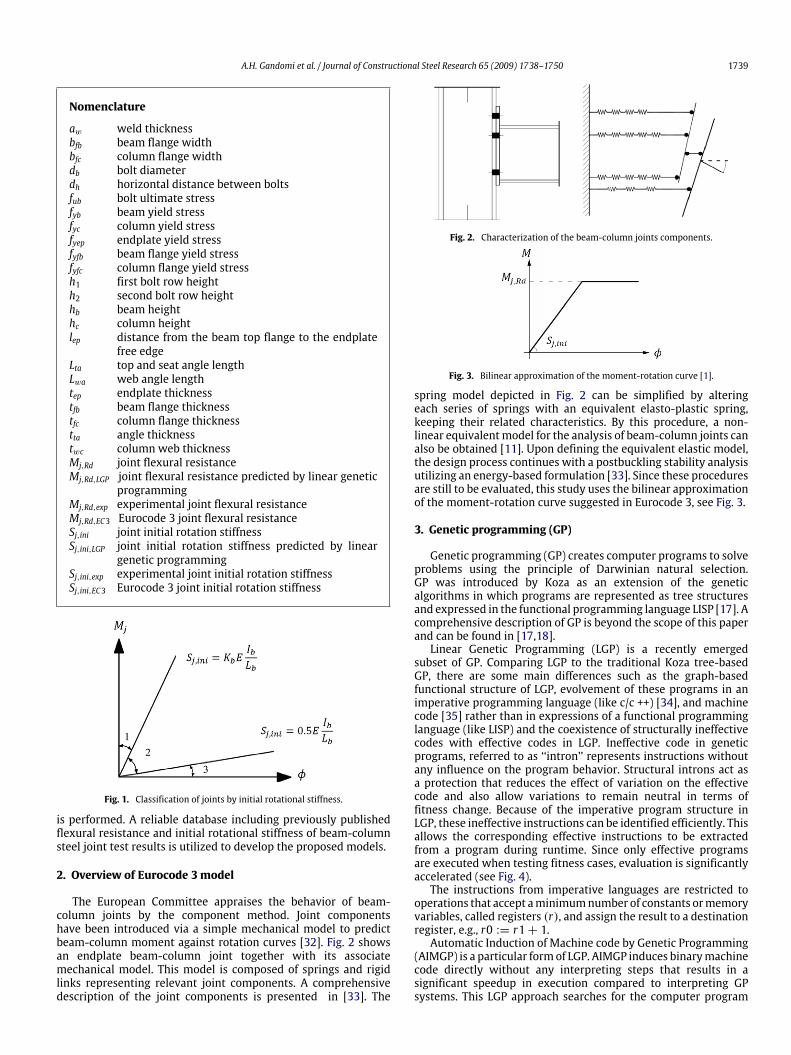
Fig. 1. Classification of joints by initial rotational stiffness.

is performed. A reliable database including previously publishedflexural resistance and initial rotational stiffness of beam-columnsteel joint test results is utilized to develop the proposed models.

2. Overview of Eurocode 3 model

The European Committee appraises the behavior of beam-column joints by the component method. Joint componentshave been introduced via a simple mechanical model to predictbeam-column moment against rotation curves [32]. Fig. 2 showsan endplate beam-column joint together with its associatemechanical model. This model is composed of springs and rigidlinks representing relevant joint components. A comprehensivedescription of the joint components is presented in [33]. The

Fig. 2. Characterization of the beam-column joints components.

Fig. 3. Bilinear approximation of the moment-rotation curve [1].

spring model depicted in Fig. 2 can be simplified by alteringeach series of springs with an equivalent elasto-plastic spring,keeping their related characteristics. By this procedure, a non-linear equivalentmodel for the analysis of beam-column joints canalso be obtained [11]. Upon defining the equivalent elastic model,the design process continues with a postbuckling stability analysisutilizing an energy-based formulation [33]. Since these proceduresare still to be evaluated, this study uses the bilinear approximationof the moment-rotation curve suggested in Eurocode 3, see Fig. 3.

3. Genetic programming (GP)

Genetic programming (GP) creates computer programs to solveproblems using the principle of Darwinian natural selection.GP was introduced by Koza as an extension of the geneticalgorithms in which programs are represented as tree structuresand expressed in the functional programming language LISP [17]. Acomprehensive description of GP is beyond the scope of this paperand can be found in [17,18].Linear Genetic Programming (LGP) is a recently emerged

subset of GP. Comparing LGP to the traditional Koza tree-basedGP, there are some main differences such as the graph-basedfunctional structure of LGP, evolvement of these programs in animperative programming language (like c/c ++) [34], and machinecode [35] rather than in expressions of a functional programminglanguage (like LISP) and the coexistence of structurally ineffectivecodes with effective codes in LGP. Ineffective code in geneticprograms, referred to as ‘‘intron’’ represents instructions withoutany influence on the program behavior. Structural introns act asa protection that reduces the effect of variation on the effectivecode and also allow variations to remain neutral in terms offitness change. Because of the imperative program structure inLGP, these ineffective instructions can be identified efficiently. Thisallows the corresponding effective instructions to be extractedfrom a program during runtime. Since only effective programsare executed when testing fitness cases, evaluation is significantlyaccelerated (see Fig. 4).The instructions from imperative languages are restricted to

operations that accept aminimumnumber of constants ormemoryvariables, called registers (r), and assign the result to a destinationregister, e.g., r0 := r1+ 1.Automatic Induction of Machine code by Genetic Programming

(AIMGP) is a particular formof LGP. AIMGP induces binarymachinecode directly without any interpreting steps that results in asignificant speedup in execution compared to interpreting GPsystems. This LGP approach searches for the computer program

1740 A.H. Gandomi et al. / Journal of Constructional Steel Research 65 (2009) 1738–1750

PopulationIntron

EliminationFitness

Evaluation

Effective Program

Individual

Fig. 4. Elimination of non-effective code in LGP. Only effective programs areexecuted [29].

and the constants at the same time. The evolved program is asequence of binary machine instructions [35]. The machine-code-based, LGP uses the following steps to evolve a computer programthat predicts the target output from a data file of inputs andoutputs [29,36]:Step 1: Initializing a population of randomly generated

programs.Step 2: Running a tournament. In this step four programs are

randomly selected from the population. They are compared andbased on their fitness; two programs are picked as winners andtwo as losers.Step 3: Transforming the winner programs. The two winner

programs are copied and transformed probabilistically as follows:Parts of the winner programs are exchanged with each other tocreate two new programs (crossover operation); and/or each ofthe tournament winners are changed randomly to create two newprograms (mutation operation).Step 4: Replacing the loser programs in the tournament with

the transformedwinner programs. The winners of the tournamentremain unchanged.Step 5: Repeating steps two to four until convergence. A

program defines the output of the algorithm that simulates thebehavior of the problem to an arbitrary degree of accuracy.Other details of LGP and a comprehensive description on LGP

parameters can be obtained in [29]. Based on the numericalexperiments LGP has the ability to significantly outperform similartechniques and can be utilized as an efficient alternative to thetraditional Koza tree-based GP [29–31].

4. Model development

Six different models are developed for the prediction of flexuralresistance and initial rotational stiffness of three kinds of semi-rigid joints (bolted endplate joints, welded joints and bolted jointswith angles) using LGP. In all models, the input parameters arethe geometrical characteristics and mechanical properties. It is

noteworthy that the input and output parameters needed formodel development are normalized between 0.05 and 0.95 beforethe learning process. These models use 60% of the total data fortraining, 20% of the total data for validation and the remaining 20%for testing. Other details for developing the models including thedatabase description are presented in following subsections.

4.1. Bolted endplate joints

The required data was collected for the development of twoLGP models to predict the flexural resistance and initial rotationalstiffness of bolted endplate joints. The collected experimental dataincluded 26 bolted endplate joints found in [2,4,7–10]. Sixteenvariables were used as input parameters to the LGP predictivemodels as shown in Fig. 5: column flangewidth (bfc), column flangethickness (tfc), column height (hc), column yield stress (fyc), beamflange width (bfb), beam flange thickness (tfb), beam height (hb),beam yield stress (fyb), endplate thickness (tep), distance from thebeam top flange to the endplate free edge (lep), endplate yieldstress (fyep), bolt diameter (db), bolt ultimate stress (fub), firstbolt row height (h1), second bolt row height (h2), and horizontaldistance between bolts (dh). The complete list of input data forbolted endplate joints is presented in Table 1.

4.2. Welded joints

For this type of joint, a reliable database was obtained fromthe literature to developmodels. The database contains 33 flexuralresistance and initial rotational stiffness of welded joint testresults [16], given in Table 2. The inputs for LGP, shown in Fig. 6,are: column flange width (bfc), column flange thickness (tfc),column web yield stress (fywc), column height (hc), column flangeyield stress (fyfc), beam flange width (bfb), beam flange thickness(tfb), beam height (hb), beam flange yield stress (fyfb), and weldthickness (aw).

4.3. Bolted angle joints

For bolted joints with angles, the data utilized to calibrate andvalidate the LGP models are obtained from [5,6]. The followingvariableswere used as input parameters as shown in Fig. 7: columnflange thickness (tfc), beam height (hb), angle thickness (tta), topseat angle length (Lta), web angle length (Lwa) and bolt diameter(db). The input data for this type of joints are given in Table 3.

4.4. LGP model

In order to develop LGP models capable of predicting flexuralresistance and initial rotational stiffness of every beam-column

hc

hb fub

dh

db

bfc

bfb

h2

h1

tfc

tep

tfblep

twc

Fig. 5. Extended endplate joint layout.


Table 1Input data for endplate joints.

Test bfc tfc hc fyc bfb tfb hb fyb tep lep fyep db fub h1 h2 dh

T110001 300 13.5 296 475 220 15.5 543 300 25 105 416 24 1323 580.3 474.8 30T110002 300 13.5 296 482 220 15.5 543 309 25 105 410 24 1323 580.3 474.8 30T110005 300 12.5 296 532 220 15.5 547 290 25 105 404 24 1323 584.2 478.8 30T109003 180 14.1 179 300 151 11.2 300 323 30 70 273 20 1000 334.4 244.4 46T109004 180 14 180 306 192 14 454 285 41 84 323 24 1000 496 381 65T109005 240 16.4 240 276 192 14 454 285 41 84 323 24 1000 496 381 65T109006 240 17 240 275 220 18.6 597 288 41 82 325 24 1000 634.7 514.7 62T101004 160 12.6 163 280 99.7 8.4 198.8 351 15 60 315.5 16 1000 229.6 149.6 25T101007 163 12.6 160 280 99.7 8.4 198.8 351 15 60 315.5 16 1000 229.6 149.6 25T101010 160 12.6 163 280 150.9 10.8 298.9 303 20 70 291.5 20 1000 333.5 243.5 30T101013 120 9.7 241 310 99.7 8.4 198.8 351 18 60 330.5 16 1000 229.6 149.6 24T101014 151 10.8 299 303 99.7 8.4 198.8 351 15 60 327 16 1000 229.6 149.6 25T839 240 12 230 256 180 13.5 400 235 12 80 214 20 785 433.3 343.3 35T8310 200 15 200 243 180 13.5 400 235 14 80 312 20 980 433.3 343.3 35T8311 300 14 290 417 300 23 490 235 14 113 312 24 785 546.5 426.5 60T911 301 14.4 302 317 181 14.6 401 323 30 90 266 24 980 443.7 338.7 61T912 301 14.3 302 317 181 14.4 401 317 30 90 261 24 980 443.8 338.8 61T913 301 14.5 301 279 181 14.4 401 279 30 90 239.5 24 980 443.8 338.8 61TC5 204 10.9 206 283 133.3 7.6 205.4 283 16 111.2 250 16 633 268.8 138.8 30TC6 204 10.9 206 283 133.3 7.6 205.4 283 16 111.2 250 20 980 268.8 138.8 30TC7 204 10.9 206 283 133.3 7.6 205.4 283 20 111.2 250 16 633 268.8 138.8 30TC8 204 10.9 206 283 133.3 7.6 205.4 283 20 111.2 250 20 980 268.8 138.8 30TC9 204 10.9 206 283 133.3 7.6 205.4 283 16 111.2 250 16 633 268.8 138.8 30TC10 204 10.9 206 283 133.3 7.6 205.4 283 16 111.2 250 20 980 268.8 138.8 30TC11 204 10.9 206 283 133.3 7.6 205.4 283 20 111.2 250 16 633 268.8 138.8 30TC12 204 10.9 206 283 133.3 7.6 205.4 283 20 111.2 250 20 980 268.8 138.8 30

Geometrical characteristics are in mm and mechanical properties are in MPa.

Table 2Input data for welded joints.

Test bfc tfc twc hc fyfc bfb tfb hb fyfb aw

T107001 178 8.9 6.2 173 334.6 119 10.2 238 389.8 6.8T107002 179 8.8 6.2 175 342.5 149 10 300 306.2 5.8T107003 242 10.7 9.4 233 354.2 149 10 300 304.8 9.1T107004 242 10.8 11.3 233 343.9 190 13.2 452 287 11.3T105002 160 13.3 7.6 159 260 162 11.4 328 286 7.5T105003 179 13.5 9 183 288 149 10 298 334 7T105004 179 13.4 8.2 183 277 180 12.3 398 284 9.3T105005 200 13.9 8.4 202 273 171 10.7 361 271 7.2T105006 239 16 9.7 239 276 223 18.1 604 306 10.3T105007 299 18.6 11.7 300 296 181 13.2 400 309 9.1T105008 301 19.3 12.4 297 292 300 17.8 301 357 13T105009 139 11.5 7.7 139 300 110 10 218 312 6.2T105010 138 11.6 7.8 146 281 111 9.1 221 361 6.2T105011 140 12 7.5 142 298 151 11.1 302 304 6.4T105014 178 13.7 8.1 177 292 170 12.3 359 290 7.5T105015 179 13.5 9.4 178 275 180 12.5 397 290 10.2T105016 200 14.6 9.4 200 279 171 12 361 273 8.9T105018 240 16.1 9.7 239 269 189 14.1 451 284 10.1T105019 239 16.3 10.1 240 274 224 18.7 605 322 8.6T105020 299 18.3 10.8 298 301 210 17.2 551 268 11.9T105021 299 18.9 12.3 303 266 220 19.4 600 268 11.6T105023 301 18.7 12 302 276 299 22.9 402 281 12.1T105024 300 18 10.6 298 271 301 27.6 500 271 12.7T105025 301 21.3 11.9 361 276 224 18.2 604 316 11.4T106001 145 21.4 13.2 159 283 149 11 295 358 11.8T106002 186 22.8 14.5 200 265 177 13.5 398 358 12.1T106003 204 25.4 15.9 221 268 180 12.6 401 265 11T106004 204 25.6 15.9 222 267 199 15.1 498 248 14T106005 204 24.5 16 222 280 224 18.7 600 277 12.7T106006 222 25 16.5 241 278 209 18 552 361 13.5T106007 308 37 21.2 340 237 300 28 603 262 14.2T108032 199 15 9 199 370 186 13.1 450 386 4T108038 202 12 8.7 209 291 168 12.5 361 307 5.5T108042 255 18.5 12.2 265 267 200 15.5 498 288 5.7

Geometrical characteristics are in mm and mechanical properties are in MPa.

steel joints, two separate models with a single output weredeveloped; one for flexural resistance and one for initial rotationalstiffness. The various parameters involved in the LGP models are:population size, mutation rate and its different types, crossoverrate, homologous crossover, function set, number of demes and

program size. The parameter selection will affect the modelgeneralization capability of LGP. They were selected, after a trialand error approach, upon some previously suggested values [37,38]. The parameter settings are shown in Table 4. In the analysis,the data sets were divided into training, validation and testing


twc

hctfc

tfb

hbaw

twc

bfc

bfb

Fig. 6. Welded joint layout.

lta

hb

tfc

lwa

hc

db

tta

Fig. 7. Bolted angle joint.

Table 3Input data for bolted joints with angles (in mm).

Test tfc hb tta Lta Lwa db

8S1 16.3 209.6 9.5 88.9 139.7 168S2 16.3 209.6 9.5 88.9 139.7 168S3 16.3 209.6 7.9 88.9 139.7 168S4 16.3 209.6 9.5 152.4 139.7 168S5 16.3 209.6 9.5 101.6 139.7 168S6 16.3 209.6 7.9 101.6 139.7 168S7 16.3 209.6 9.5 101.6 139.7 168S8 16.3 209.6 7.9 88.9 139.7 22.28S9 16.3 209.6 9.5 88.9 139.7 22.28S10 16.3 209.6 12.7 88.9 139.7 22.214S1 22.9 358.8 9.5 101.6 215.9 1614S2 22.9 358.8 12.7 101.6 215.9 1614S3 22.9 358.8 9.5 101.6 139.7 1614S4 22.9 358.8 9.5 101.6 215.9 1614S5 22.9 358.8 9.5 101.6 215.9 22.214S6 22.9 358.8 12.7 101.6 215.9 22.214S8 22.9 358.8 15.9 101.6 215.9 22.214S9 22.9 358.8 12.7 101.6 215.9 22.2

Geometrical characteristics are in mm.

subsets as mentioned earlier. Prior to training, the data werenormalized as:

Xn =0.9Xi − 0.05Xi,min + 0.95Xi,max

Xi,max − Xi,min. (1)

This way the data lie between 0.05 and 0.95. Xi,min and Xi,max arerespectively the minimum and maximum values of Xi; and Xn isthe normalized value. For LGP modeling, Discipulus software [37],

Table 4Parameter settings for LGP.

Parameter Settings

Population size 2000–10000Maximum program size 256Initial program size 80Crossover rate 0.5, 0.95Homologous crossover 0.95Mutation rate 0.9Block mutation rate 0.3Instruction mutation rate 0.3Data mutation rate 0.4Function set +, -, *, /,

√, sin, cos, tan

Number of demes 20

based on the AIMGP approach, was used. After completing aproject, in addition to the creation of single solutions, they arecombined into team solutions [39] to produce better results. Thedeveloped programs were written in Java, C, or Intel assemblercode. The resulting code can be compiled into a DLL or COMobject and called from the optimization routines [40]. In order toevaluate the capabilities of LGP models, the correlation coefficient(R), mean absolute percent error (MAPE), and root mean squarederror (RMSE) were used as the criteria between the actual andpredicted values.

5. Discussion of results

Fig. 8(a–f) displays the predicted flexural resistance versusthe experimental flexural resistance of different types of joints


(a) LGP Single Solution-Endplate joints. (b) LGP Team Solution-Endplate joints. (c) LGP Single Solution-Welded joints.

(d) LGP Team Solution-Welded joints. (e) LGP Single Solution-Bolted joints with angles. (f) LGP Team Solution-Bolted joints with angles.

Fig. 8. Comparison of predicted vs experimental flexural resistance using LGP single and team solutions.

Fig. 9. Relative comparison of predicted flexural resistance of endplate joints.

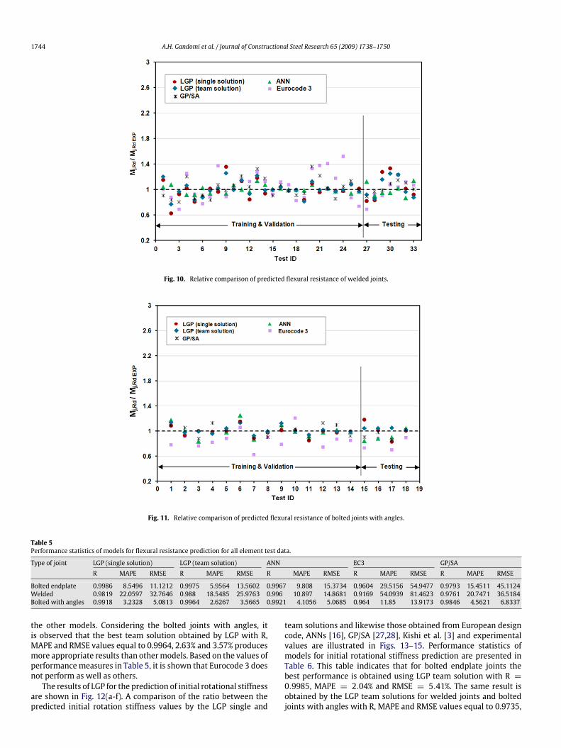
obtained by LGP single and team solutions. A comparison of theratio between predicted flexural resistance values by the LGP,as well as those obtained from the European design code [1],ANNs [16], GP/SA [27,28] and experimental values are shownin Figs. 9–11. As mentioned previously, R, MAPE and RMSEare selected as the target statistical parameters to evaluate the

performance of models. Considering the R, MAPE and RMSE valuesfor flexural resistance, given in Table 5, it can be seen that the bestperformance for bolted endplate joints is obtained by LGP singlesolution (R = 0.9986, MAPE = 8.55%, RMSE = 11.12%). For theprediction of flexural resistance of welded joints, ANNs model(R = 0.996, MAPE = 10.90%, RMSE = 14.87%) outperforms


Fig. 10. Relative comparison of predicted flexural resistance of welded joints.

Fig. 11. Relative comparison of predicted flexural resistance of bolted joints with angles.

Table 5Performance statistics of models for flexural resistance prediction for all element test data.

Type of joint LGP (single solution) LGP (team solution) ANN EC3 GP/SAR MAPE RMSE R MAPE RMSE R MAPE RMSE R MAPE RMSE R MAPE RMSE

Bolted endplate 0.9986 8.5496 11.1212 0.9975 5.9564 13.5602 0.9967 9.808 15.3734 0.9604 29.5156 54.9477 0.9793 15.4511 45.1124Welded 0.9819 22.0597 32.7646 0.988 18.5485 25.9763 0.996 10.897 14.8681 0.9169 54.0939 81.4623 0.9761 20.7471 36.5184Bolted with angles 0.9918 3.2328 5.0813 0.9964 2.6267 3.5665 0.9921 4.1056 5.0685 0.964 11.85 13.9173 0.9846 4.5621 6.8337

the other models. Considering the bolted joints with angles, itis observed that the best team solution obtained by LGP with R,MAPE and RMSE values equal to 0.9964, 2.63% and 3.57% producesmore appropriate results than othermodels. Based on the values ofperformancemeasures in Table 5, it is shown that Eurocode 3 doesnot perform as well as others.The results of LGP for the prediction of initial rotational stiffness

are shown in Fig. 12(a-f). A comparison of the ratio between thepredicted initial rotation stiffness values by the LGP single and

team solutions and likewise those obtained from European designcode, ANNs [16], GP/SA [27,28], Kishi et al. [3] and experimentalvalues are illustrated in Figs. 13–15. Performance statistics ofmodels for initial rotational stiffness prediction are presented inTable 6. This table indicates that for bolted endplate joints thebest performance is obtained using LGP team solution with R =0.9985, MAPE = 2.04% and RMSE = 5.41%. The same result isobtained by the LGP team solutions for welded joints and boltedjoints with angles with R, MAPE and RMSE values equal to 0.9735,


(a) LGP Single Solution-Endplate joints (b) LGP Team Solution-Endplate joints

(c) LGP Single Solution-Welded joints (d) LGP Team Solution-Welded joints

(e) LGP Single Solution-Bolted joints with angles

(f) LGP Team Solution-Bolted joints with angles

Horizontal axis represents predicted initial stiffness (MN.m)Horizontal axis represents predicted initial stiffness (MN.m)

Ver

tical

axi

s re

pres

ents

pre

dict

ed in

itial

stif

fnes

s (M

N.m

)V

ertic

al a

xis

repr

esen

ts p

redi

cted

initi

al s

tiffn

ess

(MN

.m)

Fig. 12. Comparison of predicted vs. experimental initial rotational stiffness using LGP single and team solutions.

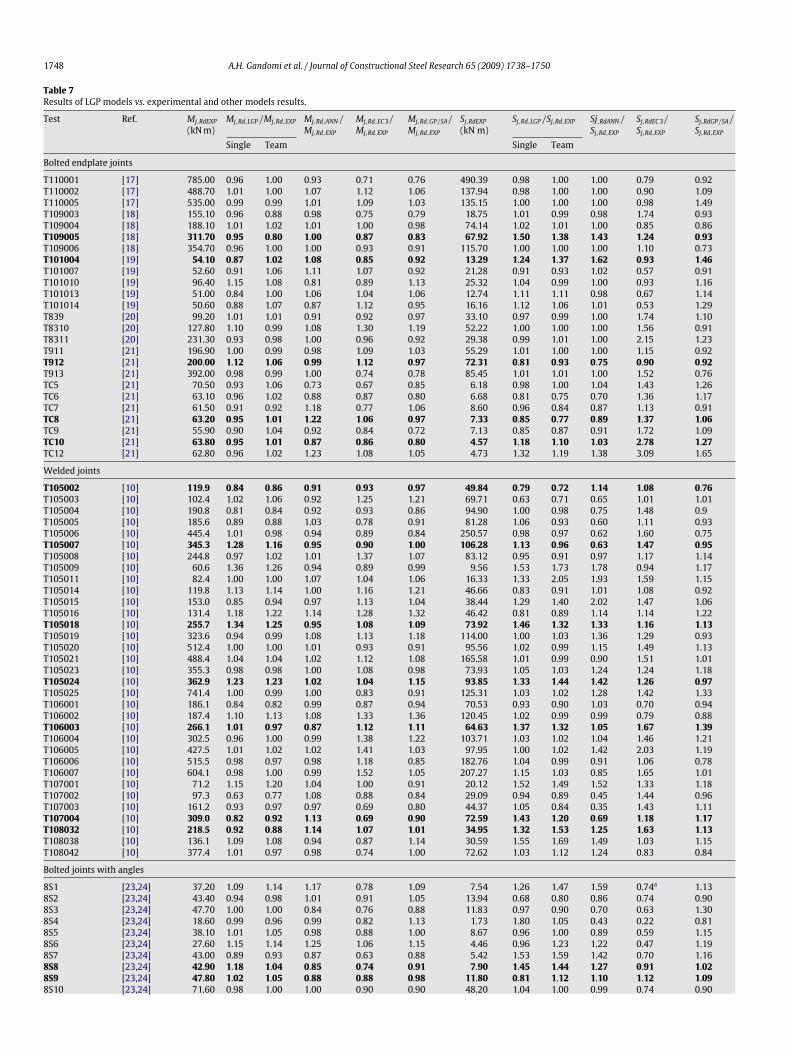
9.35%, 12.85% and 0.9923, 1.73%, 2.22%, respectively. Table 7of theappendix shows a comparative analysis of results.In order to evaluate the number of times each input appears in

the contribution of the fitness of the LGP programs (importanceof input parameters), frequency [37] values of input parametersof the flexural resistance and initial rotational stiffness predictivemodels are obtained and presented in Figs. 16–18. A value of 1.00in the figures indicates that the input variable appeared in 100%

of the best thirty programs evolved by LGP. According to Fig. 16,for endplate joints, flexural resistance is more sensitive to columnflange width (bfc) and bolt ultimate stress (fub); while for initialrotation stiffness they are endplate yield stress (fyep) and secondbolt row height (h2). Considering the welded joints, it can be seenfrom Fig. 17 that beam height (hb) and column height (hc) are themost influencing parameters on flexural resistance; and those forinitial rotation stiffness are beam height (hb) and weld thickness


Fig. 13. Relative comparison of predicted initial rotation stiffness of endplate joints.

Fig. 14. Relative comparison of predicted initial rotation stiffness of welded joints.

Table 6Performance statistics of models for initial rotation stiffness prediction for all element test data.

Type of joint LGP (single solution) LGP (team solution) ANN EC3 GP/SAR MAPE RMSE R MAPE RMSE R MAPE RMSE R MAPE RMSE R MAPE RMSE

Bolted endplate 0.9969 3.2788 7.6883 0.9985 2.0408 5.4111 0.9973 2.578 7.0930 0.9778 17.0412 25.7569 0.9836 3.6232 17.7062Welded 0.9734 9.9467 14.1824 0.9735 9.347 12.8468 0.8546 21.2279 28.0037 0.9455 32.3606 48.3830 0.9490 10.2478 17.7226Bolted with angles 0.9901 1.88 2.3452 0.9923 1.7272 2.2249 0.9923 1.7433 2.0616 0.9271a 6.1606a 7.9737a 0.9784 1.3071 3.4205a Kishi et al. model.

(aw). As shown in Fig. 18, flexural resistance of bolted joints withangles is more sensitive to angle thickness (tta) and top and seatangle length (Lta) while those for initial rotational stiffness areangle thickness (tta) and web angle length (Lwa) compared to theother inputs.

6. Conclusions

The first application of a particular subset of GP, namelyLGP, to the flexural resistance and initial rotational stiffness

prediction of semi-rigid joints, and its performance comparisonswere presented. The LGP-based models were developed uponavailable experimental results. The geometrical characteristics andmechanical properties of joints were utilized as inputs. The LGPresults were compared to the experimental results, as well asEurocode 3 and other existing models in the literature. In order todetermine the contribution of each input in the models, frequencyvalues of different input parameters of the flexural resistance andinitial rotational stiffness predictive models were also evaluated.Based on the values of performancemeasures, it was observed that


Fig. 15. Relative comparison of predicted initial rotation stiffness of bolted joints with angles.

1.0

0.9

0.8

0.7

0.6

0.5

0.4

0.3

0.2

0.1

0.0bfc tfc hc fyc bfb tfb hb fyb tep lep fyep db fub h1 h2 dh

Flexural Resistance

Initial Rotational Stiffness

Fig. 16. Frequency values of input parameters of endplate joints predictive models.

1.0

0.9

0.8

0.7

0.6

0.5

0.4

0.3

0.2

0.1

0.0bfc tfc twc hc fyfc bfb tfb hb fyfb aw

Flexural Resistance

Initial Rotational Stiffness

Fig. 17. Frequency values of input parameters of welded joints predictive models.

the proposed LGP models give very reliable estimates of flexuralresistance and initial rotational stiffness of beam-column steeljoints. The results roughly demonstrate that the best single andteam solutions created by LGP were more accurate than ANNmodels and far more accurate than Eurocode 3 and the othermodels. Furthermore, the LGP team solutions produced slightlybetter results than the single solutions except for the prediction of

flexural resistance of bolted endplate joints. It was found that theLGP based models yielded better results for the prediction of bothflexural resistance and initial rotational stiffness of bolted endplatejoints than those of bolted joints with angles and welded joints.Because of the high precision of the models developed by the LGPapproach, an excessive number of experiments and computationscan be avoided, which leads to reduction of the costs of product


Table 7Results of LGP models vs. experimental and other models results.

Test Ref. Mj,RdEXP(kNm)

Mj,Rd,LGP/Mj,Rd,EXP Mj,Rd,ANN/Mj,Rd,EXP

Mj,Rd,EC3/Mj,Rd,EXP

Mj,Rd,GP/SA/Mj,Rd,EXP

Sj,RdEXP(kN m)

Sj,Rd,LGP/Sj,Rd,EXP Sj,RdANN/Sj,Rd,EXP

Sj,RdEC3/Sj,Rd,EXP

Sj,RdGP/SA/Sj,Rd,EXP

Single Team Single Team

Bolted endplate joints

T110001 [17] 785.00 0.96 1.00 0.93 0.71 0.76 490.39 0.98 1.00 1.00 0.79 0.92T110002 [17] 488.70 1.01 1.00 1.07 1.12 1.06 137.94 0.98 1.00 1.00 0.90 1.09T110005 [17] 535.00 0.99 0.99 1.01 1.09 1.03 135.15 1.00 1.00 1.00 0.98 1.49T109003 [18] 155.10 0.96 0.88 0.98 0.75 0.79 18.75 1.01 0.99 0.98 1.74 0.93T109004 [18] 188.10 1.01 1.02 1.01 1.00 0.98 74.14 1.02 1.01 1.00 0.85 0.86T109005 [18] 311.70 0.95 0.80 1.00 0.87 0.83 67.92 1.50 1.38 1.43 1.24 0.93T109006 [18] 354.70 0.96 1.00 1.00 0.93 0.91 115.70 1.00 1.00 1.00 1.10 0.73T101004 [19] 54.10 0.87 1.02 1.08 0.85 0.92 13.29 1.24 1.37 1.62 0.93 1.46T101007 [19] 52.60 0.91 1.06 1.11 1.07 0.92 21.28 0.91 0.93 1.02 0.57 0.91T101010 [19] 96.40 1.15 1.08 0.81 0.89 1.13 25.32 1.04 0.99 1.00 0.93 1.16T101013 [19] 51.00 0.84 1.00 1.06 1.04 1.06 12.74 1.11 1.11 0.98 0.67 1.14T101014 [19] 50.60 0.88 1.07 0.87 1.12 0.95 16.16 1.12 1.06 1.01 0.53 1.29T839 [20] 99.20 1.01 1.01 0.91 0.92 0.97 33.10 0.97 0.99 1.00 1.74 1.10T8310 [20] 127.80 1.10 0.99 1.08 1.30 1.19 52.22 1.00 1.00 1.00 1.56 0.91T8311 [20] 231.30 0.93 0.98 1.00 0.96 0.92 29.38 0.99 1.01 1.00 2.15 1.23T911 [21] 196.90 1.00 0.99 0.98 1.09 1.03 55.29 1.01 1.00 1.00 1.15 0.92T912 [21] 200.00 1.12 1.06 0.99 1.12 0.97 72.31 0.81 0.93 0.75 0.90 0.92T913 [21] 392.00 0.98 0.99 1.00 0.74 0.78 85.45 1.01 1.01 1.00 1.52 0.76TC5 [21] 70.50 0.93 1.06 0.73 0.67 0.85 6.18 0.98 1.00 1.04 1.43 1.26TC6 [21] 63.10 0.96 1.02 0.88 0.87 0.80 6.68 0.81 0.75 0.70 1.36 1.17TC7 [21] 61.50 0.91 0.92 1.18 0.77 1.06 8.60 0.96 0.84 0.87 1.13 0.91TC8 [21] 63.20 0.95 1.01 1.22 1.06 0.97 7.33 0.85 0.77 0.89 1.37 1.06TC9 [21] 55.90 0.90 1.04 0.92 0.84 0.72 7.13 0.85 0.87 0.91 1.72 1.09TC10 [21] 63.80 0.95 1.01 0.87 0.86 0.80 4.57 1.18 1.10 1.03 2.78 1.27TC12 [21] 62.80 0.96 1.02 1.23 1.08 1.05 4.73 1.32 1.19 1.38 3.09 1.65

Welded joints

T105002 [10] 119.9 0.84 0.86 0.91 0.93 0.97 49.84 0.79 0.72 1.14 1.08 0.76T105003 [10] 102.4 1.02 1.06 0.92 1.25 1.21 69.71 0.63 0.71 0.65 1.01 1.01T105004 [10] 190.8 0.81 0.84 0.92 0.93 0.86 94.90 1.00 0.98 0.75 1.48 0.9T105005 [10] 185.6 0.89 0.88 1.03 0.78 0.91 81.28 1.06 0.93 0.60 1.11 0.93T105006 [10] 445.4 1.01 0.98 0.94 0.89 0.84 250.57 0.98 0.97 0.62 1.60 0.75T105007 [10] 345.3 1.28 1.16 0.95 0.90 1.00 106.28 1.13 0.96 0.63 1.47 0.95T105008 [10] 244.8 0.97 1.02 1.01 1.37 1.07 83.12 0.95 0.91 0.97 1.17 1.14T105009 [10] 60.6 1.36 1.26 0.94 0.89 0.99 9.56 1.53 1.73 1.78 0.94 1.17T105011 [10] 82.4 1.00 1.00 1.07 1.04 1.06 16.33 1.33 2.05 1.93 1.59 1.15T105014 [10] 119.8 1.13 1.14 1.00 1.16 1.21 46.66 0.83 0.91 1.01 1.08 0.92T105015 [10] 153.0 0.85 0.94 0.97 1.13 1.04 38.44 1.29 1.40 2.02 1.47 1.06T105016 [10] 131.4 1.18 1.22 1.14 1.28 1.32 46.42 0.81 0.89 1.14 1.14 1.22T105018 [10] 255.7 1.34 1.25 0.95 1.08 1.09 73.92 1.46 1.32 1.33 1.16 1.13T105019 [10] 323.6 0.94 0.99 1.08 1.13 1.18 114.00 1.00 1.03 1.36 1.29 0.93T105020 [10] 512.4 1.00 1.00 1.01 0.93 0.91 95.56 1.02 0.99 1.15 1.49 1.13T105021 [10] 488.4 1.04 1.04 1.02 1.12 1.08 165.58 1.01 0.99 0.90 1.51 1.01T105023 [10] 355.3 0.98 0.98 1.00 1.08 0.98 73.93 1.05 1.03 1.24 1.24 1.18T105024 [10] 362.9 1.23 1.23 1.02 1.04 1.15 93.85 1.33 1.44 1.42 1.26 0.97T105025 [10] 741.4 1.00 0.99 1.00 0.83 0.91 125.31 1.03 1.02 1.28 1.42 1.33T106001 [10] 186.1 0.84 0.82 0.99 0.87 0.94 70.53 0.93 0.90 1.03 0.70 0.94T106002 [10] 187.4 1.10 1.13 1.08 1.33 1.36 120.45 1.02 0.99 0.99 0.79 0.88T106003 [10] 266.1 1.01 0.97 0.87 1.12 1.11 64.63 1.37 1.32 1.05 1.67 1.39T106004 [10] 302.5 0.96 1.00 0.99 1.38 1.22 103.71 1.03 1.02 1.04 1.46 1.21T106005 [10] 427.5 1.01 1.02 1.02 1.41 1.03 97.95 1.00 1.02 1.42 2.03 1.19T106006 [10] 515.5 0.98 0.97 0.98 1.18 0.85 182.76 1.04 0.99 0.91 1.06 0.78T106007 [10] 604.1 0.98 1.00 0.99 1.52 1.05 207.27 1.15 1.03 0.85 1.65 1.01T107001 [10] 71.2 1.15 1.20 1.04 1.00 0.91 20.12 1.52 1.49 1.52 1.33 1.18T107002 [10] 97.3 0.63 0.77 1.08 0.88 0.84 29.09 0.94 0.89 0.45 1.44 0.96T107003 [10] 161.2 0.93 0.97 0.97 0.69 0.80 44.37 1.05 0.84 0.35 1.43 1.11T107004 [10] 309.0 0.82 0.92 1.13 0.69 0.90 72.59 1.43 1.20 0.69 1.18 1.17T108032 [10] 218.5 0.92 0.88 1.14 1.07 1.01 34.95 1.32 1.53 1.25 1.63 1.13T108038 [10] 136.1 1.09 1.08 0.94 0.87 1.14 30.59 1.55 1.69 1.49 1.03 1.15T108042 [10] 377.4 1.01 0.97 0.98 0.74 1.00 72.62 1.03 1.12 1.24 0.83 0.84

Bolted joints with angles

8S1 [23,24] 37.20 1.09 1.14 1.17 0.78 1.09 7.54 1.26 1.47 1.59 0.74a 1.138S2 [23,24] 43.40 0.94 0.98 1.01 0.91 1.05 13.94 0.68 0.80 0.86 0.74 0.908S3 [23,24] 47.70 1.00 1.00 0.84 0.76 0.88 11.83 0.97 0.90 0.70 0.63 1.308S4 [23,24] 18.60 0.99 0.96 0.99 0.82 1.13 1.73 1.80 1.05 0.43 0.22 0.818S5 [23,24] 38.10 1.01 1.05 0.98 0.88 1.00 8.67 0.96 1.00 0.89 0.59 1.158S6 [23,24] 27.60 1.15 1.14 1.25 1.06 1.15 4.46 0.96 1.23 1.22 0.47 1.198S7 [23,24] 43.00 0.89 0.93 0.87 0.63 0.88 5.42 1.53 1.59 1.42 0.70 1.168S8 [23,24] 42.90 1.18 1.04 0.85 0.74 0.91 7.90 1.45 1.44 1.27 0.91 1.028S9 [23,24] 47.80 1.02 1.05 0.88 0.88 0.98 11.80 0.81 1.12 1.10 1.12 1.098S10 [23,24] 71.60 0.98 1.00 1.00 0.90 0.90 48.20 1.04 1.00 0.99 0.74 0.90


Table 7 (continued)

Test Ref. Mj,RdEXP(kNm)

Mj,Rd,LGP/Mj,Rd,EXP Mj,Rd,ANN/Mj,Rd,EXP

Mj,Rd,EC3/Mj,Rd,EXP

Mj,Rd,GP/SA/Mj,Rd,EXP

Sj,RdEXP(kN m)

Sj,Rd,LGP/Sj,Rd,EXP Sj,RdANN/Sj,Rd,EXP

Sj,RdEC3/Sj,Rd,EXP

Sj,RdGP/SA/Sj,Rd,EXP

Single Team Single Team

14S1 [23,24] 77.70 1.02 1.13 1.10 0.79 1.06 22.03 1.10 1.10 1.10 0.65 1.0114S2 [23,24] 107.00 1.01 1.00 1.00 1.21 1.03 33.33 0.99 0.97 0.95 1.12 1.2014S3 [23,24] 73.90 0.84 1.06 0.91 0.70 0.86 13.09 1.32 1.37 1.16 1.10 1.0614S4 [23,24] 92.90 0.85 0.94 0.92 0.94 0.89 25.07 0.97 0.97 0.97 0.57 0.8914S5 [23,24] 86.20 1.00 1.02 0.98 0.75 1.13 27.90 0.88 0.96 0.98 0.61 0.8014S6 [23,24] 119.00 0.98 1.00 1.02 0.87 1.10 32.30 0.99 1.01 1.02 1.39 1.2414S8 [23,24] 176.40 1.00 0.99 0.99 0.85 0.93 65.40 0.99 0.99 1.01 1.22 0.9614S9 [23,24] 115.70 1.01 1.02 1.05 0.90 1.03 29.20 1.10 1.11 1.12 1.54 1.14a Kishi et al. model; Bold sets are test sets.

Flexural Resistance Initial Rotational Stiffness1.0

0.9

0.8

0.7

0.6

0.5

0.4

0.3

0.2

0.1

0.0tfc hb tta Lta Lwa db

Fig. 18. Frequency values of input parameters of bolted joints with angles predictive models.

development. In addition, LGP unlike most models is a white-boxmodel that provides transparent programs of an imperative ormachine language [41].

References

[1] CEN, Eurocode 3. May 2003 EN1993-1-8: Design of Joints. CEN, EuropeanCommittee for Standardization Brussels, Brussels, p. 124.

[2] Zoetemeijer P, Munter H. Extended endplate with disappointing rotationcapacity: Test results and analysis. Report [6-75-20 KV-4]. University ofTechnology, Delft. 1983.

[3] Kishi N, Chen WF, Matsuoka KG. Moment-rotation relation of top-and-seatangle with double web angle joints. In: Joints in steel structures. 1987.p. 121–134.

[4] Janss J, Jaspart JP, Maquoi R. Experimental study of non-linear behaviour ofbeam-to-column bolted joints. Joints in steel structures: Behaviour, strengthand design. In: Proceedings of the 1st international workshop on joints. 1997.

[5] Azizinamini A, Bradburn JH, Radziminski J. Initial stiffness of semi-rigid steelbeam-to-column joints. Journal of Constructional Steel Research 1987;8:71–90.

[6] Azizinamini A, Radziminski J. Static and cyclic performance of semi-rigidsteel beam-to-column joints. Journal of Structural Engineering 1989;115(12):2979–99.

[7] Simek I, Wald F. Test results on endplate beam-to-column joints. G-1121Report. Czech Technical University, Prague, 1991.

[8] Aggarwal AK. Comparative tests on end plate beam-to-column joints. Journalof Constructional Steel Research 1994;30(2):151–75.

[9] Faella C, Piluso V, Rizzano G. Structural steel semi-rigid joints - theory, designand software. CRC Press; 1999. p. 505.

[10] Hummer C, Tschemmernegg T. A non-linear joint model for the design ofstructural steel frames. Costruzioni Metalliche, No. 1. 1988.

[11] Simões R, Simões da Silva L, Cruz P. Behaviour of endplate beam-to-columncomposite joints under cyclic loading. Steel Composite Structure 2001;1(3):355–76.

[12] Haykins S. Neural networks –A comprehensive foundation. 2nd ed. EnglewoodCliffs (NJ): Prentice Hall International Inc.; 1999.

[13] Abdala KM. Stavroulakis, back propagation neural network model for semi-rigid joints. Microcomputers in Engineering 1995;10(2):77–87.

[14] Stavroulakis GE, Abdala KM. A systematic neural network classificator inmechanics. application in semi-rigid steel joints. International Journal ofEngineering Analysis and Design 1994;1:279–92.

[15] Anderson D, Hines EL, Arthur SJ, Eiap EL. Application of artificial neuralnetworks to the prediction of minor axis joints. Computers & Structures 1997;63(4):685–92.

[16] de Lima LRO, da S, Vellasco PCG, de Andrade SAL, da Silva JGS, Vellasco MMBR.Neural networks assessment of beam-to-column joints. Journal of theBrazilian Society of Mechanical Sciences 2005;27(3):314–24.

[17] Koza JR. Genetic programming: On the programming of computers by meansof natural selection. Cambridge (MA): MIT Press; 1992.

[18] Banzhaf W, Nordin P, Keller R, Francone F. Genetic programming – anintroduction. In: On the automatic evolution of computer programs and itsapplication. Heidelberg/San Francisco: dpunkt/Morgan Kaufmann; 1998.

[19] Bäck T. Evolutionary algorithms in theory and practice: Evolution strategies,evolutionary programming, genetic algorithms. USA: Oxford University Press;1996.

[20] Ashour AF, Alvarez LF, Toropov VV. Empiricalmodelling of shear strength of RCdeep beams by genetic programming. Computers & Structures 2003;81(55):331–8.

[21] Alavi AH, Gandomi AH, Gandomi M, Sahab MG. A data mining approachto compressive strength of CFRP confined concrete cylinders. Computers &Structures, 2008 [in press].

[22] Javadi AA, Rezani M, Mousavi Nezhad M. Evaluation of liquefaction inducedlateral displacements using genetic programming Computers andGeotechnics2006;33(4–5):222–33.

[23] Folino G, Pizzuti C, Spezzano G. Genetic Programming and simulatedAnnealing: A hybrid method to evolve decision trees. In: Poli R, Banzhaf W,Langdon WB, Miller JF, Nordin P, Fogarty TC, editors. Genetic programming,proceedings of EuroGP’2000, vol. 1802. Edinburgh: Springer-Verlag; 2000.p. 294–303.

[24] Metropolis N, Rosenbluth AW, Rosenbluth MN, Teller AH, Teller E. Equation ofstate calculations by fast computing mechanics. Journal of Chemical Physics1953;21(6):1087–92.

[25] Kirkpatrick Jr S, Gelatt CD, Vecchi MP. Optimization by simulated annealing.Science 1983;220(4598):671–80.

[26] Cerny V. Thermodynamical approach to the traveling salesman problem:an efficient simulation algorithm. Journal of Optimization Theory andApplications 1985;45:41–52.

[27] Gandomi AH, Sahab MG, Heshmati AA, Alavi AH, Gandomi M, Arjmandi P.Application of a coupled simulated annealing-genetic programming algorithmto the prediction of bolted joints behavior. American-Eurasian Journal ofScientific Research 2008;3(2):153–62.

[28] Gandomi AH, Alavi AH, Sahab MG, Gandomi M, Safari Gorji M. Empiricalmodels for Prediction of flexural resistance and initial stiffness of weldedbeam-column joints. In: 11th East Asia-Pacific conference on structuralengineering & construction, 2008.

[29] Brameier M, Banzhaf W. Linear Genetic Programming. Springer Science +Business Media, LLC; 2007.

[30] Oltean M, Grosan C. A comparison of several linear genetic programmingtechniques. Complex Systems 2003;14(4):1–29.

[31] Baykasoğlu A, Güllü H, Çanakçı H, Özbakır L. Prediction of compressive andtensile strength of limestone via genetic programming. Expert Systems withApplication 2008;35(1-2):111–23.

[32] Jaspart JP. Recent advances in the field of steel joints-column bases andfurther configurations for beam-to-column joints and beam splices. Chercheurqualifié du F.N.R.S., Universite de Liege, Faculte des Sciences Appliques 1997.


[33] Da Silva LS, Coelho AMG. Ductility model for steel joints. Journal ofConstructional Steel Research 2001;57(1):45–70.

[34] Brameier M, Kantschik W, Dittrich P, Banzhaf W. SYSGP – A C++ library ofdifferent GP variants. Technical Report [CI-98/48]; Germany: CollaborativeResearch Ceter 531 University of Dortmund, 1998.

[35] Nordin PJ. A compiling genetic programming system that directlymanipulatesthe machine code. In: Kenneth E, Kinnear JR, editors. Advances in GeneticProgramming. USA: MIT Press; 1994. p. 311–31. (Chapter 14).

[36] Deschaine LM. Tackling real-world environmental challenges with lineargenetic programming. PCAI magazine 2000;15(5):35–7.

[37] Francone F. DiscipulusTMowner’s manual. In: Version 3.0, Register MachineLearning Technologies. 2000.

[38] Feldt R, Nordin P. Using factorial experiments to evaluate the effect of geneticprogramming parameters. In: EuroGP 2000. LNCS, vol. 1802. 2000. p. 271–82.

[39] Brameier M, Banzhaf W. Evolving teams of predictors with linear geneticprogramming. Genetic Programming and Evolvable Machines 2001;2(4):381–407.

[40] Francone FD, Deschaine LM. Extending the boundaries of design optimizationby integrating fast optimization techniques with machine-code-based lineargenetic programming. Information Sciences 2004;161(3–4):99–120.

[41] Weise T. Global optimization algorithms — Theory and application. On-line E-book, GNU free documentation license (FDL). 2007. Available at:http://www.it-weise.de/projects/book.pdf.

http://www.it-weise.de/projects/book.pdf

Behavior appraisal of steel semi-rigid joints using Linear Genetic Programming

Documents

Transcript of Behavior appraisal of steel semi-rigid joints using Linear Genetic Programming