Monte Carlo Market Greeks in the Displaced Diffusion Libor ...

MONTE CARLO MARKET GREEKS IN THE DISPLACEDDIFFUSION LIBOR MARKET MODEL

MARK S. JOSHI AND OH KANG KWON

Abstract. The problem of developing sensitivities of exotic interest ratesderivatives to the observed implied volatilities of caps and swaptions isconsidered. It is shown how to compute these from sensitivities to modelvolatilities in the displaced diffusion LIBORmarket model. The exampleof a cancellable inverse floater is considered.

JEL codes: C15, [email protected]

1. Introduction

The LIBOR market model (lmm) is a standard model for pricing exoticinterest rate derivatives, particularly for those with early termination fea-tures, and Monte Carlo simulation is the most common method of its imple-mentation in practice. Consequently, there have been significant advancesin efficient Monte Carlo implementation of the LMM, and the calculationof corresponding Monte Carlo sensitivities, see for example Joshi (2003),Glasserman and Zhao (1999) and Giles and Glasserman (2006). Much ofthe work on sensitivities, however, focuses on model rather than market sen-sitivities. That is, existingmethods consider sensitivities to quantities such asinitial LIBORs and LIBOR volatilities rather than sensitivities to quantitiessuch as futures/swap rates and cap/swaption volatilities. Yet it is the latterthat are of greater importance to traders and risk managers, since they areinterested in price responses to directly observed market movements ratherthan responses to parameters resulting from, and depending on, calibrationmethods employed.

In this paper, we introduce for the displaced diffusion lmm a Monte Carlobasedmethod for computingmarket sensitivities. Sincemarket-quoted quan-tities affect prices only indirectly through the calibrated model parameters,the key problem lies in translatingmovements inmarket-quoted quantities tocorresponding movements in model parameters. In general, simply “bump-ing” a market-quoted quantity and recalibrating to obtain the “bumped”model parameters is undesirable since practitioners often use calibrations

Date: November 8, 2010.Key words and phrases. LIBOR market model, calibration, Greeks, vegas.

1

2 MARK S. JOSHI AND OH KANG KWON

based on semi-global optimizations,1 and such approaches result in unpre-dictable movements to model parameters that, in turn, result in unreliablesensitivities.

There appears to have been very little discussion of this problem in theliterature. Piterbarg (2004) discusses the use of volatility scenarios. Brace(2007) looks at the problem of computing swaption vegas using matrix in-version.

The difficulty in the problem lies in the fact that when we compute thesensitivity to a given swaption volatility, we wish to perturb in such a waythat the other calibrated instruments’ prices remain invariant. A swaptionvega is thus not just an attribute of the calibration and the swaption but also ofthe set of swaptions and caps chosen. This reflects the fact from elementarycalculus that a partial derivative is only defined in terms of what else is heldconstant.

The approach introduced in this paper takes as given a base calibration,representing model parameters resulting from the calibration of implemen-tor’s choice, and defines for each market- quoted quantity a new calibrationthat is in some sense a minimal perturbation of the base calibration. Thekey point to note is that the new parameters are computed relative to baseparameters, by perturbation, and not completely afresh from a bump-and-recalibrate type procedure. This results in a more efficient calculation of“bumped” model parameters, and more reliable price sensitivities.

We stress that our approach does not require recalibration for each bumpof a market-quoted quantity to determine the corresponding perturbations tomodel parameters. Moreover, the resulting perturbations to model parame-ters are minimal in a sense and hence introduce least amount of noise, re-sulting in stable sensitivities.

Whilst in this paper we focus solely on the displaced diffusion LIBORmarket model, the fast adjoint method has been developed for other marketmodels, see Joshi and Yang (2009a) and Joshi and Yang (2009b), and it isclear that similar arguments will apply to those cases.

The remainder of this paper is organized as follows. In Section 2, wereview the displaced diffusion LIBOR market model and how to computemodel vegas. We define and show how to compute market vegas in Section3. We consider the example of a cancellable inverse floater in Section 4. InAppendix A, we develop the necessary analytic formulas.

1For example, the method proposed in Pedersen (1998).

MC MARKET GREEKS IN THE DISPLACED LMM 3

2. Preliminaries

In this section we give a brief review of the displaced diffusion lmm, andadapt to this model the pathwise Greeks approach introduced in Giles andGlasserman (2006).

2.1. Displaced Diffusion LIBOR Market Model. Fix n ∈ N, an increas-ing sequence 0 < T0 < T1 < · · · < Tn ∈ R, and let τk = Tk+1 − Tk, for0 ≤ k ≤ n− 1. Denote by fk(t) the LIBOR rate over the interval (Tk, Tk+1)for 0 ≤ t ≤ Tk, and define

η(t) = min{0 ≤ k ≤ n : Tk > t}, (2.1)

so that η(t) is the index of the nearest maturing LIBOR rate at time t. Letδk ∈ R+ for 0 ≤ k < n, and define f̄k(t) = fk(t) + δk. The dynamics of thedisplaced LIBOR rates, f̄k(t) are assumed to satisfy the sdes

df̄k(t) = f̄k(t)λk(t)dt+ f̄k(t)γk(t)tdw(t), (2.2)

under the spot LIBOR measure, P, where w(t) is a standard d-dimensionalP-Wiener process, γk : R+ → Rd is the deterministic volatility for f̄k, and

λk(t) =k∑

i=η(t)

τif̄i(t)γi(t)tγk(t)

1 + τifi(t). (2.3)

Let 0 < t0 < t1 < · · · < tN be the simulation times for Monte Carlo,where without loss of generality {T0, T1, . . . , Tn} ⊂ {t0, t1, . . . , tN}, and let∆i = ti+1 − ti for 0 ≤ i ≤ N − 1. Then under the log-Euler discretizationscheme, f̄k in (2.2) are approximated by

f̄k(ti+1) ≈ f̄k(ti) e(λk(ti)− 1

2|γk(ti)|2)∆i+γk(ti)·ξi

√∆i , (2.4)

where ξi is a d-dimensional standard normal random variate. We will takethe terms γk(t) to be piecewise constant and not to vary within a step; anycalibration can be rewritten in this form.

For future reference, we define

γi = (γ1(ti), γ2(ti), . . . , γn(ti))t√

∆i, (2.5)

so that the k-th row of γi corresponds to the integrated “volatility” term forthe k-th LIBOR rate in (2.2) at time step ti.

We refer the reader to Brace (2007) for further details on the displaceddiffusion LIBOR market model where it is called “shifted BGM.”


2.2. Giles and Glasserman (2006) Greeks. For notational convenience,define fk(t) = fk(Tk) for t ≥ Tk, and let

f̄ i = (f̄1(ti), f̄2(ti), . . . , f̄n(ti))t. (2.6)

In view of the Euler scheme in (2.4), we can regard f̄ i+1 as a function of f̄ iand write

f̄ i+1 = Φi(f̄ i), (2.7)

where Φi : Rn → Rn and Φi,k(f̄ i) = f̄k(ti+1) is the k-th component of Φi.Now, consider an interest rate dependent cash flowX occurring at time tl.

For example,X may be one of the coupon payments associated with a struc-tured product. Then to compute the price sensitivities for X with respect toa model parameter, say α, which only affects step r, repeated application ofthe chain rule gives

∂X

∂α=∂X

∂f̄ l

∂f̄ l∂f̄ l−1

· · · ∂f̄ r+1

∂α. (2.8)

A key observation in Giles and Glasserman (2006) was that by comput-ing the above product backwards rather than forwards, each step involvesa matrix-by-vector multiplication rather than matrix-by-matrix multiplica-tion. This results in a reduction of the order of computation from n3 to n2 foreach step. In the case of a reduced-factor model, they managed to go furtherby using the special structure of the model and reduced the computationalorder to nd.

Giles and Glasserman only considered the case of log-normal rates; how-ever, their results were accelerated and extended to the case of displacedrates by Denson and Joshi (2009). This means that we can assume that wehave available to us a methodology for rapidly computing model Greeks. Inparticular, if D is the price of our exotic interest rate derivative today, thenwe will assume, in what follows, that we know

∂D

∂γi,jk

for all i, j and k. Our objective is to express market vegas as linear combi-nation of these model or elementary vegas.

The standard path-wise method only applies to Lipschitz continuous pay-offs. However, it is possible to extend it to the case where a jump disconti-nuity occurs across a hypersurface, see Chan and Joshi (2009).

3. Calibration and Minimal Perturbations

Note from (2.4) that an Euler discretization scheme for a displaced lmmis completely specified by the initial LIBORs, f 0, the displacements and


the pseudo-root matrices, γi, at each simulation time. In practice, the ini-tial LIBORs are usually obtained by bootstrapping market quoted rates ofvarious maturities, whilst the pseudo-roots are obtained by first fitting theLIBOR volatilities to quoted cap and/or swaption volatilities and then pos-sibly performing factor reduction. In view of this, we will refer to a set ofinitial LIBORs and pseudo-root matrices thus obtained as a base calibration,C0, of displaced lmm. Note that we do not insist on the particular bootstrap-ping method, nor do we insist on the particular LIBOR volatility calibration,for the base calibration. The perturbed calibrations we define below will berelative to the base calibration that the implementor provides.

From now on, we focus on the Euler discretization scheme (2.6) for thedisplaced diffusion lmm with n underlying LIBOR rates and driven by ad-dimensional Wiener process. Moreover, to ease notational burden we as-sume that n = N + 1 and Ti = ti, for all 0 ≤ i < n, so that LIBOR rateexpiry times and simulation times coincide. The pseudo-roots, γi, will thenbe n × d dimensional matrices with each row corresponding to a LIBORrate. However, since expired LIBORs have zero volatility, the first i rows ofγi will be zero, and the space of pseudo-root calibrations will hence consistof approximately r = 1

2n2d (possible) non-zero entries2 making up the n

pseudo-root matrices.Although it is not essential for what follows, we remark that it is actually

the covariance matrices that determine a calibration rather than the pseudo-square roots in that two different pseudo-square roots may give the samecovariance matrix and therefore the same prices to all instruments. For ex-ample, if O is an orthogonal matrix and A is a pseudo-root matrix then

AAt = AO(AO)t.

Our motivation for working with pseudo-roots is that the space of d-factorpseudo-root matrices is trivially invariant under all perturbations. This is inmarked contrast to covariance matrices where a small perturbation may leadto an increase in factors and/or a failure to be positive definite.

Since to us a calibration is a vector of pseudo-root matrices, we can, afterrearrangement, regard it as an element of Euclidean space,Rr, for some larger. We denote by vi, the non-zero pseudo-root entries regarded as elementsof Rr, ordered for example by time, row and column. Since a calibration isdetermined by forwards as well as pseudo-root matrices, our space of cali-brations is thenRr×Rn. LetX1, X2, . . . , Xm be the market-quoted impliedvolatilities from which the base calibration is determined. Within possibleLIBOR market models, the terms Xi are then functions on Rr × Rn.

2It may be the case that the chosen base calibration imposes restrictions that reduce thenumber of non-zero pseudo-root entries.


In what follows, our objective is to compute vegas and the forward rateswill be fixed. We will therefore treat the forward-rates parametrically andgenerally ignore them notationally. Now that we have identified calibrationsas elements of Rr, we have a natural distance between them which is sim-ply the Euclidean distance. With this metric, two close together calibrationswill give similar forward rate evolutions on every path of a simulation. Analternative measure of calibration distance would be to take the distance be-tween covariance matrices: however, this would have the disadvantage thatclose together calibrations would not need to have similar evolutions on apath-wise basis.

For our instruments of interest, swaptions and caps, the implied volatilitycan be computed approximately via an analytic formula. The terms Xi aretherefore given as computable functions on Rr × Rn and we can computetheir gradients as functions on Rr,

wi = ∇vXi =

(∂Xi

∂v1

,∂Xi

∂v2

, . . . ,∂Xi

∂vr

)t. (3.1)

Denote byWX the subspace of Rr spanned by these gradients so that

WX = 〈w1,w2, . . . ,wr〉R. (3.2)

Now, for computing price sensitivities, we wish to bump Xi to Xi + ε,for some ε ∈ R+, say 1 basis point, whilst holding Xj for j 6= i fixed, andto construct a corresponding calibration. As explained earlier, computingafresh the base calibration for the bumped market is unreliable. Instead, wepropose an alternative calibration, Ci, that is consistent with the bump andas close as possible to the base calibration C0. Intuitively, rather than con-sidering the bumped market completely independently of the base marketand performing recalibration, we take as given the base calibration and lookfor the nearest perturbation that is consistent with the bump. We now give aprecise definition of Ci.

Assume that we are given a base calibration C0 and let vi, where 1 ≤ i ≤ r,be the non-zero pseudo-root entries ordered in someway as described above.Define v = (v1, v2, . . . , vr)

t, and recall thatXi can be regarded as a functionof v. Provided that theXi thus considered are sufficiently smooth, (which iscertainly the case for the Hull–White approximation,) we have

Xi(v + h) = Xi(v) + 〈wi,h〉+O(|h|2), (3.3)

wherewi are as defined in (3.1) and h ∈ Rr represents a perturbation fromthe base pseudo-root entries v. For the bumpXi 7→ Xi+ε, the perturbation,h, must satisfy Xi(v + h) ≈ Xi(v) + ε, whence

〈wi,h〉 = ε. (3.4)


Moreover, since the perturbation must leave the remaining Xj fixed, we re-quire Xj(v + h) ≈ Xj(v), or equivalently

〈wj,h〉 = 0 (3.5)

for j 6= i.Since the dimensionality of the space of calibrations is usuallymuch greater

than the number of market instruments being calibrated to, these equationsare not sufficient to determine a unique perturbation h. For this reason, weimpose the additional condition that the perturbation isminimal, in the sensethat the perturbed calibration is as close to C0 as possible. Of course, the no-tion of closeness is norm dependent and we have chosen the L2-norm whichis convenient both numerically and geometrically. Hence we impose a finalconstraint on the perturbation, h,

〈h,h〉 → minimized. (3.6)

We have given a mathematical description of h, but we still need an algo-rithm to find it. To explain how the perturbation may be computed in prac-tice, we give a geometric construction. Let

Hi = 〈wj | j 6= i 〉R ⊂ Rr, (3.7)

and let H⊥i ⊂ Rr be the subspace orthogonal to Hi.We can now rewrite the three conditions determining the minimal pertur-

bation, hi, corresponding to Xi as follows:

hi ∈ H⊥i , 〈wi,hi〉 = ε, and 〈hi,hi〉 minimal. (3.8)

There is a simple geometric solution to this problem: hi lies in the linearspan of the projection ofwi ontoH⊥i .We therefore project and then linearlyscale to achieve 〈wi,hi〉 = ε. This procedure will only fail if the projectionofwi ontoH⊥i is zero. However, this is to be expected, since in that caseXi

is locally (i.e. to first order) a linear combination of the remainingXj , and itis not possible to perturb Xi while keeping Xj , for j 6= i, fixed. In practice,such redundant calibrating instruments should be discarded.

So given a base calibration C0 consisting of f 0 and v, we can computefor each Xi the corresponding perturbation, hi, and obtain the calibration,Ci consisting of f 0 and v + hi.This allows us to write the vega with respect to instrument Xi as a linear

combination of the model vegas. Our market vega is now simply

∂D

∂Xi

=1

ε

r∑j=1

hi,j∂D

∂vj,

where the terms ∂D∂vj

are the model vegas from Section 2.2 with the indicesrelabelled.


Rates 5% Rates 6% Rates 7% Rates 8% Rates 9%1.42× 10−4 1.76× 10−5 2.21× 10−6 1.58× 10−6 −1.85× 10−7

3.68× 10−4 1.13× 10−4 2.72× 10−5 5.65× 10−6 3.42× 10−6

4.47× 10−4 2.04× 10−4 7.52× 10−5 2.14× 10−5 5.20× 10−6

4.16× 10−4 2.73× 10−4 1.32× 10−4 5.78× 10−5 9.31× 10−6

3.79× 10−4 2.98× 10−4 1.78× 10−4 7.79× 10−5 2.91× 10−5

3.44× 10−4 3.08× 10−4 1.96× 10−4 1.09× 10−4 5.59× 10−5

2.89× 10−4 2.96× 10−4 2.10× 10−4 1.40× 10−4 7.07× 10−5

2.67× 10−4 2.88× 10−4 2.18× 10−4 1.46× 10−4 8.60× 10−5

1.58× 10−4 2.46× 10−4 2.37× 10−4 1.75× 10−4 9.37× 10−5

1.72× 10−4 2.20× 10−4 2.03× 10−4 1.50× 10−4 1.08× 10−4

1.50× 10−4 2.11× 10−4 1.85× 10−4 1.61× 10−4 1.18× 10−4

1.23× 10−4 1.80× 10−4 1.82× 10−4 1.58× 10−4 1.19× 10−4

1.13× 10−4 1.50× 10−4 1.53× 10−4 1.43× 10−4 1.18× 10−4

8.15× 10−5 1.22× 10−4 1.49× 10−4 1.31× 10−4 1.19× 10−4

6.28× 10−5 1.07× 10−4 1.06× 10−4 1.19× 10−4 1.06× 10−4

2.73× 10−5 6.61× 10−5 1.05× 10−4 1.10× 10−4 8.34× 10−5

4.88× 10−6 4.27× 10−5 7.13× 10−5 9.78× 10−5 9.31× 10−5

−2.80× 10−5 −8.92× 10−6 4.76× 10−5 1.29× 10−4 2.11× 10−4

−3.17× 10−5 −2.45× 10−5 −3.82× 10−5 −6.23× 10−5 −2.93× 10−5

−3.92× 10−6 −3.23× 10−5 −9.56× 10−5 −1.91× 10−4 −2.98× 10−4

Table 1. Vegas for a cancellable inverse floater with respectto co-terminal swaptions only

By construction, we have that up to order |h|2, the vega of an instrumentXi with respect to itself according to this definition agrees with the usualdefinition, and the vega of each Xi with respect to Xj for j 6= i is zero.

4. Numerical illustrations

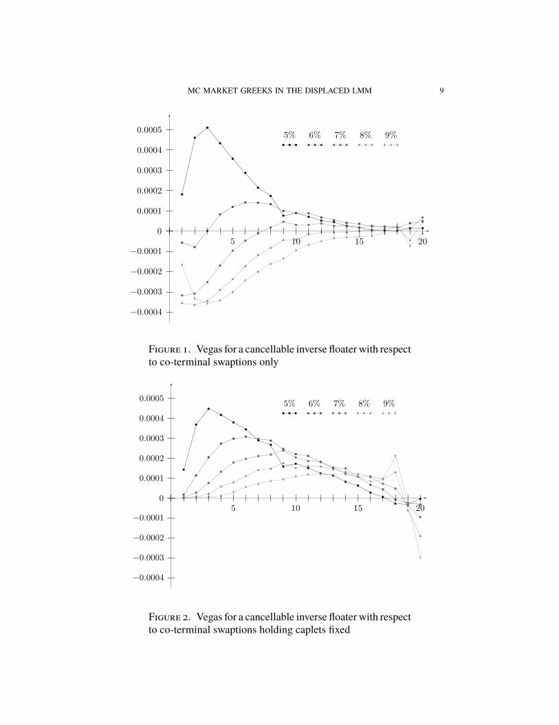
Now that we have defined the market vegas for exotic interest rate deriva-tives, it is interesting to examine their values for a particular case. We studya cancellable inverse floater swap. For this product, the issuer pays a floorleton an inverse floating LIBOR rate and receives a floating LIBOR rate. Theissuer is also able to cancel future payments on each of the payment dates.The product is therefore naturally exposed to both caplet/floorlet volatilityvia the individual payments, and swaption volatility via the right to cancelthe swap. The natural hedges are therefore caplets on the individual rates andthe co-terminal swaptions with the same underlying rates and expiry date asthe contract.


!0.0004

!0.0003

!0.0002

!0.0001

0

0.0001

0.0002

0.0003

0.0004

0.0005

5 10 15 20

5% 6% 7% 8% 9%

1

Figure 1. Vegas for a cancellable inverse floater with respectto co-terminal swaptions only

!0.0004

!0.0003

!0.0002

!0.0001

0

0.0001

0.0002

0.0003

0.0004

0.0005

5 10 15 20

5% 6% 7% 8% 9%

1

Figure 2. Vegas for a cancellable inverse floater with respectto co-terminal swaptions holding caplets fixed


Rates 5% Rates 6% Rates 7% Rates 8% Rates 9%1.81× 10−4 −5.67× 10−5 −3.17× 10−4 −3.55× 10−4 −1.66× 10−4

4.61× 10−4 −7.89× 10−5 −3.09× 10−4 −3.64× 10−4 −3.33× 10−4

5.10× 10−4 1.56× 10−6 −2.51× 10−4 −3.44× 10−4 −3.56× 10−4

4.33× 10−4 8.31× 10−5 −1.69× 10−4 −2.90× 10−4 −3.42× 10−4

3.57× 10−4 1.19× 10−4 −9.65× 10−5 −2.37× 10−4 −3.01× 10−4

2.87× 10−4 1.41× 10−4 −4.65× 10−5 −1.72× 10−4 −2.4× 10−4

2.14× 10−4 1.40× 10−4 −1.03× 10−5 −1.17× 10−4 −2.00× 10−4

1.74× 10−4 1.33× 10−4 1.82× 10−5 −8.25× 10−5 −1.62× 10−4

7.65× 10−5 9.95× 10−5 4.64× 10−5 −4.37× 10−5 −1.35× 10−4

8.94× 10−5 8.88× 10−5 3.09× 10−5 −4.23× 10−5 −9.48× 10−5

7.04× 10−5 8.78× 10−5 3.07× 10−5 −1.52× 10−5 −6.73× 10−5

5.18× 10−5 6.73× 10−5 3.73× 10−5 −4.59× 10−6 −4.98× 10−5

4.48× 10−5 5.40× 10−5 2.54× 10−5 −5.17× 10−6 −3.49× 10−5

2.50× 10−5 4.12× 10−5 2.86× 10−5 −5.60× 10−6 −2.98× 10−5

1.76× 10−5 3.61× 10−5 1.63× 10−5 4.11× 10−7 −2.60× 10−5

5.00× 10−6 2.53× 10−5 2.59× 10−5 7.04× 10−6 −2.31× 10−5

2.63× 10−6 2.29× 10−5 2.01× 10−5 1.03× 10−5 −1.02× 10−5

2.40× 10−6 1.78× 10−5 2.08× 10−5 2.08× 10−5 3.29× 10−5

1.51× 10−5 3.89× 10−5 1.17× 10−5 −4.63× 10−5 −7.33× 10−5

1.47× 10−5 4.98× 10−5 6.72× 10−5 4.32× 10−5 −1.15× 10−5

Table 2. Vegas for a cancellable inverse floater with respectto co-terminal swaptions holding caplets fixed

To facilitate reproduction of our results, we take a simple base calibrationand product. We have

Tj = 0.5(j + 1), for j = 0, . . . , 20.

The issuer pays(K − 2fk(Tk))+τ − fk(Tk)τ

at time Tk+1 where τ = 0.5.We value the product from the issuer’s perspec-tive.

We take all rates to have 0.0 displacement and constant volatility at level18%. Before factor reduction, the correlation between rate i and rate j is

L+ (1− L)e−β|Ti−Tj |,

with L = 0.5 and β = 0.2.We reduce to five factors by setting all eigenval-ues after the first 5 to zero, and then rescaling to obtain a correlation matrix.

We consider two sets of possible vega instruments. For set A, we take theat-the-money co-terminal swaptions with underlying times Tj. For set B,we take the set A together with the at-the-money caplets on the individual


Rates 5% Rates 6% Rates 7% Rates 8% Rates 9%2.07× 10−5 −3.58× 10−5 −1.61× 10−4 −1.75× 10−4 −7.48× 10−5

5.20× 10−5 −9.72× 10−5 −2.34× 10−4 −2.53× 10−4 −1.69× 10−4

6.09× 10−5 −1.37× 10−4 −2.77× 10−4 −3.02× 10−4 −2.35× 10−4

5.47× 10−5 −1.61× 10−4 −3.04× 10−4 −3.34× 10−4 −2.81× 10−4

4.10× 10−5 −1.78× 10−4 −3.20× 10−4 −3.56× 10−4 −3.14× 10−4

2.24× 10−5 −1.91× 10−4 −3.30× 10−4 −3.69× 10−4 −3.36× 10−4

3.34× 10−6 −2.01× 10−4 −3.36× 10−4 −3.78× 10−4 −3.52× 10−4

−1.70× 10−5 −2.10× 10−4 −3.39× 10−4 −3.81× 10−4 −3.63× 10−4

−3.24× 10−5 −2.18× 10−4 −3.41× 10−4 −3.84× 10−4 −3.69× 10−4

−4.67× 10−5 −2.22× 10−4 −3.40× 10−4 −3.82× 10−4 −3.71× 10−4

−5.94× 10−5 −2.26× 10−4 −3.38× 10−4 −3.79× 10−4 −3.71× 10−4

−6.97× 10−5 −2.28× 10−4 −3.35× 10−4 −3.75× 10−4 −3.69× 10−4

−7.87× 10−5 −2.27× 10−4 −3.29× 10−4 −3.69× 10−4 −3.64× 10−4

−8.51× 10−5 −2.23× 10−4 −3.23× 10−4 −3.62× 10−4 −3.59× 10−4

−8.89× 10−5 −2.18× 10−4 −3.11× 10−4 −3.53× 10−4 −3.53× 10−4

−8.69× 10−5 −2.07× 10−4 −3.00× 10−4 −3.43× 10−4 −3.44× 10−4

−7.87× 10−5 −1.90× 10−4 −2.82× 10−4 −3.31× 10−4 −3.36× 10−4

−5.72× 10−5 −1.55× 10−4 −2.56× 10−4 −3.30× 10−4 −3.62× 10−4

−2.32× 10−5 −9.75× 10−5 −1.91× 10−4 −2.74× 10−4 −3.35× 10−4

Table 3. Vegas for a cancellable inverse floater with respectto caplets holding co-terminal swaptions fixed

forward rates. Since the last caplet and co-terminal swaption are the same,we have the last caplet twice but only consider it once when computing. Thismeans that the cardinality of A is 20 and that of B is 39.

In order to minimize noise, we run 220 − 1 Sobol paths using a log-Eulerapproximation with one step per reset using the spot measure. We com-pute the exercise strategy using the extension to the least-squares methodof Carrière (1996) and Longstaff and Schwartz (2001), discussed in Amin(2003) and Joshi (2006). We hold the exercise strategy fixed when comput-ing Greeks as is usually done. We use quadratic polynomials in the first for-ward rate, the contiguous co-terminal swap-rate and the final zero-couponbond as basis functions. We use 65,536 training paths. The duality gaps aredeveloped using 256 inner and outer paths with the Joshi (2006) method.

We use five different flat yield curves varying the level of rates. In casej the initial forward rates are (4 + j)%. The discount factor for time 0.5 is0.95 in all cases. The lower bound estimates are

0.0926, 0.2113, 0.3256, 0.4192.


!0.0004

!0.0003

!0.0002

!0.0001

0

0.0001

0.0002

0.0003

0.0004

0.0005

5 10 15 20

5% 6% 7% 8% 9%

1

Figure 3. Vegas for a cancellable inverse floater with respectto caplets holding co-terminal swaptions fixed

The duality gaps to the upper bounds are

0.0064, 0.0024, 0.0012, 0.0006.

For set A, we present the results in Table 1 and Figure 1. For set B, wepresent the swaption vegas in Table 2 and Figure 2, and the caplet vegasin Table 3 and Figure 3. The value of ε used in the calculation of vegas is0.01. Thus we are showing the effect of a one-percent change in the impliedvolatility.

We see some striking differences in the swaption vegas according towhetherthe caplets are held fixed. When caplets are fixed, the swaption vegas arealmost all positive reflecting the increased value of the cancellability. Thecaplet vegas are generally negative on the other hand reflecting the fact thatthe product pays floorlets. When we consider the swaptions alone, these twoeffects merge and the swaption vegas are often negative.

5. Conclusion

We have developed a new methodology for computing sensitivities tomarket-quoted implied volatilities in the displaced diffusion LIBOR mar-ket model. We have seen that the swaption Greeks of a cancellable inversefloater vary greatly according to whether the caplets are held constant.


Appendix A. Analytic formulas and approximations

We require the gradient of the implied volatility as a function of the pseudo-root elements. In this appendix, we develop formulas for its entries. Forswaptions, we must use an analytic approximation to the implied volatil-ity and differentiate that. For caps, there is the different complication thatthe implied volatility is found by first pricing all underlying caplets and thenfinding the single constant volatility that matches their total price. We alsohave the issue that for displaced diffusion models the implied volatility isgenerally defined as the input to a log-normal (i.e. zero displacement) modelthat matches the price correctly, whereas the pseudo-root elements are de-fined for displaced log rates. So even for caplets the computation is not triv-ial.

We first discuss the algorithm for caps. (Caplets are a special case.) Let acap C have underlying rates fα, . . . , fβ with α ≤ β. The displaced impliedvolatility of one of the caplets, Cm, comprising C is given by the simpleformula

σ̂m =

√1

Tm

∑i≤m,f

γ2i,mf .

We thus have∂σ̂m∂γi,mf

=γi,mfTmσ̂m

,

for i ≤ m. Note that γi,mf = 0 for i > m. Each pseudo-root element willunderlie at most one of the caplets, so the derivative of the price of C withrespect to γi,mf is equal to that of Cm. Thus

∂C

∂γi,mf=

∂Cm∂γi,mf

= VegaD(Cm)γi,mfTmσ̂m

(A.1)

where VegaD denotes the sensitivity with respect to volatility in the dis-placed Black formula, and is given by√

Tm(fm + δm)N ′(d1)

where N is the cumulative normal function, and

d1 =log(fm+δmK+δm

)+ 0.5σ̂2

mTm

σ̂m√Tm

,

where K is the strike of the cap.We thus have the gradient of the price as a function of the underlying

pseudo-root elements. However, it is the gradient of the (log-normal) impliedvolatility that is required. Let σ̂C be the cap’s implied volatility (computed


via a numerical root search). We have∂C

∂γi,mf=

dC

dσ̂C

∂σ̂C∂γi,mf

.

Since dCdσ̂C

is computable as a sum of caplet vegas, rearranging, we obtain asimple expression for ∂σ̂C

∂γi,mfas desired.

For swaptions, we use a modification of the Hull and White (2000) an-alytic approximation. The modification is required in that we need the log-normal implied volatility in a displaced diffusion model. We proceed viacoefficient freezing. We do not consider drifts in the derivation since in thepricing measure obtained by taking the annuity as numeraire, the swap-ratewill be a martingale.We consider a swaption on a rate SRα,β with underlyingrates fα, . . . , fβ.We can write up to drift terms,

d log SRα,β =

β∑i=α

∂ log SRα,β

∂ log(fi + δi)d log(fi + δi). (A.2)

Expanding the logs, we obtain

d log SRα,β =

β∑i=α

fi + δiSRα,β

∂SRα,β

∂(fi + δi)d log(fi + δi). (A.3)

Clearly,∂SRα,β

∂(fi + δi)=∂SRα,β

∂fi.

So we have approximately,

d log SRα,β =

β∑i=α

fi + δiSRα,β

∂SRα,β

∂fi

∑f

γif (t)dwf (t).

LetZi =

fi(0) + δiSRα,β(0)

∂SRα,β

∂fi(0),

and our coefficient-frozen approximation is then

d log SRα,β =

β∑i=α

d∑f=1

Ziγif (t)dwf (t).

From this we obtain an expression for the total variance, Vα,β, of log SRα,β

as a function of γk,if which can be differentiated:

Vα,β =∑k≤α

d∑f=1

(β∑i=α

Ziγk,if

)2

.


The derivative of

σ̂α,β =

√1

TαVα,β

with respect to any element γk,if is now straight-forward to compute. Wenote that expressions for the terms ∂SRα,β

∂fican be found in Jäckel and Rebon-

ato (2003), and that these do not involve γk,if .Whilst we have used the Hull–White approximation, here, we note that

our main construction does not depend on this choice, and any analytic ap-proximation that can be straight-forwardly differentiated could be used.

ReferencesAmin, A. (2003), ‘Multi-factor cross currency Libor market models: implementation, cali-

bration and examples’, SSRN eLibrary .Brace, A. (2007), Engineering BGM, Chapman and Hall.Carrière, J. (1996), ‘Valuation of the early-exercise price for options using simulations and

nonparametric regression’, Insurance: Mathematics and Economics 19(1), 19–30.Chan, J. H. and Joshi, M. (2009), ‘Fast Monte-Carlo Greeks for Financial Products With

Discontinuous Pay-Offs’, SSRN eLibrary .Denson, N. and Joshi, M. (2009), ‘Flaming logs’, The Wilmott Journal 1(5–6), 259–262.Giles, M. and Glasserman, P. (2006), ‘Smoking adjoints: fast Monte Carlo Greeks’, Risk

January, 88–92.Glasserman, P. and Zhao, X. (1999), ‘Fast Greeks by simulation in forward LIBORmodels’,

Journal of Computational Finance 3(1), 5–39.Hull, J. and White, A. (2000), ‘Forward rate volatilities, swap rate volatilities and the im-

plementation of the LIBOR market model’, Journal of Fixed Income 10, 46–62.Jäckel, P. and Rebonato, R. (2003), ‘The link between caplet and swaption volatilities in a

Brace-Gatarek-Musiela/Jamshidian framework: approximate solutions and empiricalevidence ’, Journal of Computational Finance 6(4).

Joshi,M. (2003), ‘Rapid Computation of Drifts in a Reduced Factor LIBORMarketModel’,Wilmott Magazine 3, 84–85.

Joshi, M. (2006), ‘Monte Carlo bounds for callable products with non-analytic break costs’,SSRN eLibrary .

Joshi, M. and Yang, C. (2009a), ‘Efficient Greek Estimation in Generic Market Models’,SSRN eLibrary .

Joshi, M. and Yang, C. (2009b), ‘Fast Delta Computations in the Swap-RateMarketModel’,SSRN eLibrary .

Longstaff, F. and Schwartz, E. (2001), ‘Valuing American options by simulation: a simpleleast-squares approach ’, The Review of Financial Studies 14, 113–147.

Pedersen, M. B. (1998), ‘Calibrating Libor Market Models’, SSRN eLibrary .Piterbarg, V. (2004), ‘Pricing and hedging callable Libor exotics in forward Libor models’,

Journal of Computational Finance 8, 65–117.


Centre for Actuarial Studies, Department of Economics, University of Mel-bourne, Victoria 3010, Australia

E-mail address: [email protected]

Quantitative Applications, ANZ, Level 2, 20 Martin Place, Sydney NSW 2000,Australia

E-mail address: [email protected]

Monte Carlo Market Greeks in the Displaced Diffusion Libor ...

Documents

Transcript of Monte Carlo Market Greeks in the Displaced Diffusion Libor ...