ORIGINAL ARTICLE

doi:10.1111/evo.14377

Displaced clines in an avian hybrid zone(Thamnophilidae: Rhegmatorhina) withinan Amazonian interfluveGlaucia Del-Rio,1,2,3 Marco A. Rego,1,2 Bret M. Whitney,1,4 Fabio Schunck,4 Luís F. Silveira,4

Brant C. Faircloth,1,2 and Robb T. Brumfield1,2

1Museum of Natural Science, Louisiana State University, Baton Rouge, Louisiana 708032Department of Biological Sciences, Louisiana State University, Baton Rouge, Louisiana 70803

3E-mail: glaucia.ornito@gmail.com4Museu de Zoologia, Universidade de São Paulo, São Paulo, SP 04263-000, Brazil

Received December 20, 2020

Accepted September 1, 2021

Secondary contact between species often results in the formation of a hybrid zone, with the eventual fates of the hybridizing

species dependent on evolutionary and ecological forces. We examine this process in the Amazon Basin by conducting the first

genomic and phenotypic characterization of the hybrid zone formed after secondary contact between two obligate army-ant-

followers: the White-breasted Antbird (Rhegmatorhina hoffmannsi) and the Harlequin Antbird (Rhegmatorhina berlepschi). We

found a major geographic displacement (∼120 km) between the mitochondrial and nuclear clines, and we explore potential hy-

potheses for the displacement, including sampling error, genetic drift, and asymmetric cytonuclear incompatibilities. We cannot

exclude roles for sampling error and genetic drift in contributing to the discordance; however, the data suggest expansion and

unidirectional introgression of hoffmannsi into the distribution of berlepschi.

KEY WORDS: Antbirds, asymmetric introgression, introgressive hybridization, moving hybrid zone.

Hybrid zones are geographically limited regions of introgressive

hybridization found at the interface of two or more biological dis-

tributions. They are aptly characterized as natural laboratories of

speciation (Hewitt 1988) because they provide an opportunity to

study, in wild populations of organisms, the evolutionary and eco-

logical dynamics associated with hybridization after secondary

contact. Inferences about the evolutionary forces that generate

and maintain the structure of a hybrid zone can be made by char-

acterizing and analyzing genomic and phenotypic patterns from

a set of samples spanning the zone (Szymura and Barton 1986).

These same analyses allow inferences concerning the ultimate

fate of the hybrid zone, which includes reticulation of the two

taxa into a single taxon, genetic swamping of one taxon by the

other, or formation of an equilibrium hybrid zone.

Most hybrid zone analyses are conducted within the con-

ceptual framework of cline theory. After secondary contact with

hybridization occurs between differentiated taxa, clinal charac-

ter transitions develop across the hybrid zone as their genomes

and phenotypes recombine. If there is no selection against hy-

brids, the initially steep clines in the zone should decay at a

rate proportional to the dispersal rate (Endler 1977; Barton and

Gale 1993), eventually vanishing into a reticulate species (Endler

1977). Alternatively, if there are asymmetries in population den-

sities, dispersal ability, or competition, genetic swamping of one

of the hybridizing species will occur. Clines from loci through-

out the genome are not expected to have similar cline widths and

centers, because recombination breaks up linked parental allele

combinations.

If there is selection against hybrids, the conceptual theory

associated with the widely adopted (McEntee et al. 2020) ten-

sion zone hybrid zone model (Barton and Gale 1993) can be used

to make inferences about the forces structuring the zone. A cen-

tral component of the tension zone model is that a stable hybrid

zone is possible through the opposing forces of reduced hybrid

1© 2021 The Authors. Evolution © 2021 The Society for the Study of Evolution.Evolution

G. DEL-RIO ET AL.

fitness, which narrows the zone, and the influx of parentals,

which widens the zone. All genetic clines in tension zones are ex-

pected to have similar geographic centers and widths. This expec-

tation is based on an assumption of coupling (Butlin and Smadja

2018) in which barrier loci occur throughout the genome and the

physical and epistatic linkages among them extend their effects

to the entire genome. As the number and genomic distribution of

barrier loci decreases, the effect of coupling also decreases, and

one would expect greater variance in the centers and widths of

character clines.

Geographically, tension zones, even at equilibrium, are ex-

pected to move due to stochastic forces such as genetic drift. The

geographic landscape is not an explicit part of the model. How-

ever, tension zones, regardless of whether they are at equilibrium,

are expected to move to a point where the number of parentals

dispersing into the zone is equivalent between the species. This

often occurs at an ecotone or environmental bottleneck where the

densities of the two species are similar. In the tension zone liter-

ature, this area is often referred to as a population density trough.

Tension zones would also be expected to move if the hybridiza-

tion is due to a biological invasion, in which case the zone moves

toward the invadee as its genome becomes asymmetrically in-

tegrated into the invader (Currat et al. 2008). Beyond dispersal

dynamics, other asymmetries, such as in hybrid fitness, can also

lead to hybrid zone movements, including displacement of cyto-

plasmic and nuclear cline centers from one another (Toews and

Brelsford 2012).

Direct tests of hybrid fitness in avian hybrid zones have only

been achieved in a handful of logistically challenging studies

(Bronson et al. 2005). Thus, most inferences about hybrid fitness

are made indirectly, such as by the presence of displaced clines

or particular genotypes in the hybrid zone. For example, a pre-

ponderance of F1 individuals at the hybrid zone center suggests

hybrids are sterile or that backcrosses suffer from reduced hybrid

fitness (Pulido-Santacruz et al. 2018; Cronemberger et al. 2020);

otherwise the center is expected to be a hybrid swarm com-

posed entirely of advanced generation hybrids and backcrosses

(Harrison 1993).

Here, we present the first genetic and phenotypic char-

acterization of a hybrid zone between two obligate army-ant-

followers in southern Amazonia: the White-breasted Antbird

(Rhegmatorhina hoffmannsi) and the Harlequin Antbird (Rheg-

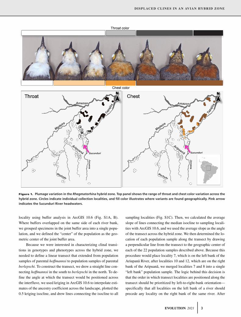
matorhina berlepschi). The two species are easily distinguishable

by their chest and throat colors: hoffmannsi has a white chest and

throat, whereas berlepschi has a rufous brown chest and a black

throat. Their entire distributions occur within the interfluve of

the Madeira and Tapajós Rivers, two of the Amazon river’s ma-

jor tributaries (Fig. 1). Rhegmatorhina berlepschi is found from

the west bank of the middle and lower Tapajós River, west to the

east bank of the Sucunduri River, then south to near the Sucun-

duri headwaters. Rhegmatorhina hoffmannsi occupies the region

between the east bank of the Madeira River and the west bank of

the Sucunduri River, then south to well beyond the headwaters of

the Sucunduri and extending eastward to an unknown extent east

of the middle Juruena River. Until field observations by BMW in

2004 revealed the presence of birds with intermediate plumage

near the Sucunduri River, it was unclear whether the two species

came into secondary contact.

Our primary goals were to characterize the genotypic and

phenotypic structure of the Rhegmatorhina hybrid zone by con-

ducting geographic and genomic cline analyses, demographic

modeling, and analyses of the genomic composition of individ-

uals in the zone. We also assess the possibility of displaced mito-

chondrial and nuclear clines suggested by patterns of mitochon-

drial haplotypes (Ribas et al. 2018). Although they did not collect

samples from the hybrid zone, Ribas et al. (2018) found a deep

mitochondrial break within parental populations of hoffmannsi

approximately 150 km south of where BMW observed birds with

intermediate plumage—observations that could indicate discor-

dant mitochondrial and phenotypic clines. We examine whether

genetic variation in the hybrid zone is best explained by neutral

diffusion, by a nonequilibrium tension zone, or by a tension zone

at equilibrium.

Materials and MethodsSAMPLING

From 2005 to 2018, GDR, MAR, BMW, FS, and LFS collected

162 specimens spanning the transition from parental hoffmannsi

to parental berlepschi. Voucher specimens were archived at the

Louisiana State University Museum of Natural Science and the

Museu de Zoologia da Universidade de São Paulo (Table S1).

For each specimen, we prepared a round skin and preserved pec-

toral muscle, heart, and liver tissues in liquid nitrogen and 95%

ethanol. To supplement our sampling, we received loans of 35

tissue samples from the Museu Paraense Emílio Goeldi (Belém,

Brazil), 21 tissue samples from the Instituto Nacional de Pesquisa

da Amazônia (Manaus, Brazil), and five tissue samples from the

Field Museum of Natural History (Chicago, IL), bringing our to-

tal sample to 222 vouchered individuals collected from 86 locali-

ties (Table S1). We included tissue samples from three outgroups:

Rhegmatorhina melanosticta (three individuals), Rhegmatorhina

gymnops (three individuals), and Rhegmatorhina. cristata (one

individual; Table S1).

DEFINING A TRANSECT OF POPULATION SAMPLES

ACROSS THE HYBRID ZONE

We defined 22 population samples from the 86 collection lo-

calities by constructing a 35 km buffer around each specimen

2 EVOLUTION 2021

DISPLACED CLINES IN AN AVIAN HYBRID ZONE

Figure 1. Plumage variation in the Rhegmatorhina hybrid zone. Top panel shows the range of throat and chest color variation across the

hybrid zone. Circles indicate individual collection localities, and fill color illustrates where variants are found geographically. Pink arrow

indicates the Sucunduri River headwaters.

locality using buffer analysis in ArcGIS 10.6 (Fig. S1A, B).

Where buffers overlapped on the same side of each river bank,

we grouped specimens in the joint buffer area into a single popu-

lation, and we defined the “center” of the population as the geo-

metric center of the joint buffer area.

Because we were interested in characterizing clinal transi-

tions in genotypes and phenotypes across the hybrid zone, we

needed to define a linear transect that extended from population

samples of parental hoffmannsi to population samples of parental

berlepschi. To construct the transect, we drew a straight line con-

necting hoffmannsi in the south to berlepschi in the north. To de-

fine the angle at which the transect would be positioned across

the interfluve, we used kriging in ArcGIS 10.6 to interpolate esti-

mates of the ancestry coefficient across the landscape, plotted the

0.5 kriging isocline, and drew lines connecting the isocline to all

sampling localities (Fig. S1C). Then, we calculated the average

slope of lines connecting the median isocline to sampling locali-

ties with ArcGIS 10.6, and we used the average slope as the angle

of the transect across the hybrid zone. We then determined the lo-

cation of each population sample along the transect by drawing

a perpendicular line from the transect to the geographic center of

each of the 22 population samples described above. Because this

procedure would place locality 7, which is on the left bank of the

Ariupanã River, after localities 10 and 12, which are on the right

bank of the Aripuanã, we merged localities 7 and 8 into a single

“left bank” population sample. The logic behind this decision is

that the order in which transect localities are positioned along the

transect should be prioritized by left-to-right-bank orientation—

specifically that all localities on the left bank of a river should

precede any locality on the right bank of the same river. After

EVOLUTION 2021 3

G. DEL-RIO ET AL.

merging localities 7 and 8, we obtained a final number of 21 pop-

ulations along the transect (Fig. S1D; Table 1). To facilitate cline

comparisons among traits, we “zeroed” the geographic distance

axis for the transect at the point where the mitochondrial transi-

tion occurs (i.e., at the Aripuanã River), with samples north of the

river having positive values and samples south of the river having

negative values.

COLLECTION OF PLUMAGE COLOR AND

MORPHOMETRIC DATA

To characterize the phenotypic structure of the hybrid zone, we

collected mensural and colorimetric data from 184 of the 222

specimens after excluding 23 specimens in juvenile plumage and

15 specimens whose condition did not allow accurate measure-

ments (Table S1). We measured eight morphometric characters

using a dial caliper (0.1 mm precision): tail length, wing length,

tarsus length, culmen length, distance from nare to tip, and bill

base width. We tested for significant differences in these charac-

ters between sexes and between parental populations of the two

species (i.e., we compared population 1 to population 21) by vi-

sual inspection of boxplots for each group and an analysis of vari-

ance with Tukey’s Honestly Significant Difference (HSD) test to

compare pairwise mean of each factor (R Core Team 2019).

To collect data on color reflectance, we calibrated an Ul-

trascan sphere reflectance spectrophotometer (Hunter Labs, Inc.,

Reston, VA) using a pure white reflecting surface (Ocean Op-

tics white standard) and measured color reflectance from 300 to

700 nm in each of eight plumage patches: crown, mantle, rec-

trices, belly, chest, throat, wing coverts, and primaries. For each

patch, we summarized percentage reflectance by averaging three

independent measurements using pavo 2.0 (Maia et al. 2019). We

compared average plumage reflectance in males and females by

visual inspection of boxplots and an analysis of variance with

Tukey’s HSD test (R Core Team 2019).

COLLECTION AND ANALYSIS OF MITOCHONDRIAL

DATA

To characterize mitochondrial DNA structure across the hybrid

zone, we extracted DNA from 195 individuals of Rhegmatorhina

and six outgroup samples (Table S1) using Qiagen DNeasy Blood

& Tissue extraction kits (Qiagen, Valencia, CA) following the

manufacturer’s protocol. After extraction, we amplified 1041

base pairs (bp) of the mitochondrial gene NADH dehydroge-

nase subunit 2 (ND2) using primers L05215 and HTrpC (5’-

CGGACTTTAGCAGAAACTAAGAG-3’) or H06313 (Sorenson

et al. 1999) in a 25 μL PCR reaction with 2.5 μL of template

DNA (∼50 ng), 1 μL of each primer (10 mM), 1 μL of 2.5 mM

(each) dNTPs, 2.5 μL of reaction buffer with MgCl2 (15 mM),

and 0.1 U of NEB HotStart Taq DNA polymerase (5 U/μL). We

used a thermocycling profile of 94°C for 5 min, followed by 34

cycles of 94°C for 30 s, 60 s of annealing at 54°C, 60 s at 72°C,

and a 10-min final extension at 72°C. We then had a commercial

facility (Macrogen Corp.) purify PCR products with Exo-SAP

(Thermo Fisher Scientific, Inc.) and Sanger sequence (forward

and reverse) purified products using capillary electrophoresis on

an Applied Biosystems 3730xl Genetic Analyzer (Thermo Fisher

Scientific, Inc.).

We used Geneious R10 (https://www.geneious.com) to align

forward and reverse sequences to a reference R. hoffmannsi ND2

sequence (GenBank MG603845). We excluded base calls with

PHRED scores below 30, and we removed sequences of eight

individuals (Table S1) because they were shorter than the total

length of ND2. We used MUSCLE (Edgar 2004) to generate a

consensus sequence from forward and reverse sequences of each

individual, aligned consensus sequences among individuals using

Geneious Alignment (2020.1.1), and reconstructed an ND2 phy-

logenetic tree using BEAST 2 (Bouckaert et al. 2014) with the

GTR + γ finite-sites substitution model, 100 million iterations,

and sampling from the posterior distribution every 1,000 itera-

tions. We removed the first 10% of posterior samples as burn-in;

we checked convergence of the remaining posterior sample with

Tracer (Rambaut et al. 2014), considering that the run converged

when ESS values were ≥200 (Drummond et al. 2006); and we

estimated a maximum clade credibility tree with TreeAnnotator

(2.5.1). To visualize the relationships between mitochondrial hap-

lotypes and the number of mutations separating them, we con-

structed a haplotype network using the program PopART (Leigh

and Bryant 2015) with the TCS algorithm (Clement et al. 2002).

RADseq LIBRARY PREPARATION AND SEQUENCING

To investigate nuclear genetic structure and allele frequencies

for the largest possible sample of individuals across the hybrid

zone, we collected RADseq (Baird et al. 2008) data from the 222

Rhegmatorhina individuals described in the “Sampling” section.

Before preparing RADseq libraries, we evaluated the quality of

DNA extracts by visualizing each on 1.5% agarose gels, and we

considered samples having fragment lengths >1.5 kbp adequate

for library preparation. We excluded extracts from 10 samples

that fell below this size range (Table S1), and we constructed

3RAD (Bayona-Vásquez et al. 2019) libraries for the remain-

ing 212 samples using XbaI and EcoRI-HF, with NheI to reduce

formation of adapter dimers. We cleaned ligation products using

Sera-Mag Speed-Beads (Rohland and Reich 2012) at a ratio of

1.25:1 (v/v), and we created full-length libraries by amplifying

the ligation products with 11 PCR cycles using iTru5 and iTru7

as described in Glenn et al. (2017). We quantified PCR-amplified

libraries using a Qubit Fluorometer (Life Technologies, Inc.)

and checked for valid constructs by visualizing each library on

1.5% agarose gels to ensure fragment distributions spanned 300–

800 bp. After validation, we cleaned amplified libraries using

4 EVOLUTION 2021

DISPLACED CLINES IN AN AVIAN HYBRID ZONE

Table

1.

Datausedforgeo

graphic

clinean

alysis.Ave

ragepercentch

estan

dthroat

reflectance

(600

nm),av

erag

ean

cestry

coefficien

t(sNMFresu

lts),allele

freq

uen

cies

forthe

berlepschim

tDNAhap

lotype,

andallele

freq

uen

cies

forthetopfive

diagnosticlociforea

chtran

sect

locality.Ave

ragean

cestry

coefficien

tisbased

on8,77

3SN

Ps.S

ample

size

within

paren

theses.S

ample

size

foran

cestry

coefficien

teq

ual

tosample

size

forcalculationofallele

freq

uen

cies

inea

chpopulation.

Popu

latio

n

Tra

nsec

tdi

stan

ce(k

m)

Che

stre

flec

tanc

eT

hroa

tref

lect

ance

Anc

estr

yco

effi

cien

tm

tDN

ASN

P1SN

P2SN

P3SN

P4SN

P5

Wes

tof

Ari

puan

ãR

iver

1−6

1155

±4

(N=

4)36

±3

(N=

4)0.

001

±0.

00(N

=8)

0.00

0.00

0.06

0.00

0.00

0.00

2–4

9549

±5

(N=

5)37

±4

(N=

5)0.

001

±0.

02(N

=8)

0.00

0.00

0.00

0.00

0.00

0.00

3–3

6545

±7

(N=

2)31

±10

(N=

2)0.

073

±0.

03(N

=3)

0.00

0.00

0.00

0.00

0.17

0.00

4–3

2444

±2

(N=

6)34

±5

(N=

6)0.

004

±0.

01(N

=7)

0.00

0.00

0.14

0.00

0.00

0.00

5–2

7349

±4

(N=

5)27

±4

(N=

5)0.

002

±0.

05(N

=5)

0.00

0.00

0.40

0.00

0.00

0.00

6–1

9353

±2

(N=

5)37

±3

(N=

5)0.

090

±0.

02(N

=5)

0.00

0.00

0.25

0.00

0.13

0.00

7–1

0539

±0

(N=

1)31

±0

(N=

1)0.

129

±0.

00(N

=1)

0.00

0.50

0.00

0.00

0.00

0.00

8–5

548

±4

(N=

8)33

±7

(N=

8)0.

067

±0.

03(N

=10

)0.

000.

000.

000.

050.

000.

009

–19

53±

4(N

=4)

33±

7(N

=4)

0.13

2±

0.02

(N=

5)0.

000.

000.

200.

000.

000.

00B

etw

een

Ari

puan

ãan

dSu

cund

uri

100

51±

6(N

=10

)33

±8

(N=

10)

0.26

8±

0.03

(N=

11)

0.63

0.55

0.41

0.23

0.23

0.23

1173

49±

5(N

=5)

29±

2(N

=5)

0.46

9±

0.02

(N=

5)1.

000.

500.

300.

400.

100.

3812

159

45±

12(N

=14

)29

±11

(N=

14)

0.53

1±

0.02

(N=

15)

1.00

0.50

0.43

0.40

0.20

0.04

1317

1.7

52±

4(N

=4)

34±

6(N

=4)

0.56

4±

0.03

(N=

5)1.

000.

800.

400.

800.

100.

3814

183.

751

±4

(N=

2)35

±4

(N=

2)0.

480

±0.

01(N

=3)

1.00

1.00

0.17

1.00

0.00

0.17

1518

5.7

10±

5(N

=5)

3±

1(N

=5)

0.87

6±

0.04

(N=

7)1.

000.

790.

640.

790.

570.

79E

astb

ank

ofSu

cund

uriR

iver

1619

5.7

20±

11(N

=19

)16

±12

(N=

19)

0.69

8±

0.08

(N=

21)

1.00

0.71

0.57

0.55

0.52

0.43

1726

820

±10

(N=

11)

11±

8(N

=11

)0.

790

±0.

08(N

=11

)1.

000.

820.

820.

770.

550.

5918

329.

811

±2

(N=

10)

2±

0(N

=10

)0.

934

±0.

04(N

=10

)1.

001.

000.

600.

751.

001.

0019

379.

812

±2

(N=

21)

3±

1(N

=21

)0.

901

±0.

03(N

=23

)1.

000.

960.

800.

890.

831.

0020

509.

810

±2

(N=

9)2

±0

(N=

9)0.

964

±0.

03(N

=9)

1.00

0.94

0.83

0.61

0.83

0.94

2168

6.8

12±

2(N

=5)

1±

1(N

=5)

0.99

0±

0.01

(N=

8)1.

001.

001.

000.

941.

001.

00

EVOLUTION 2021 5

G. DEL-RIO ET AL.

Speed-Beads at a 1:1 ratio (v/v) and pooled all libraries. To re-

duce the total number of RADseq loci recovered, we had a com-

mercial service (Georgia Genomics Facility, Athens, GA) divide

the pool of libraries across four lanes of a Pippin Prep (Sage Sci-

ence, Beverly, MA) and perform size selection using a 1.5% dye-

free Marker K agarose gel cassette (CDF1510) set to capture frag-

ments 550 bp ± 10%. After size selection, GGF staff combined

all lanes of size-selected products and increased the concentration

of size-selected libraries by performing six cycles of PCR recov-

ery using standard Illumina P5 and P7 primers. GGF staff cleaned

the resulting reaction product, quantified the size-selected pool

using a commercial library quantification kit (F. Hoffmann-La

Roche AG, Basel, Switzerland), and prepared a 10 μM pool of

libraries for paired-end (PE) 150 bp sequencing across two lanes

of Illumina HiSeq 3000 sequencing at the Oklahoma Medical Re-

search Foundation (Oklahoma City, OK).

WHOLE GENOME SEQUENCING

Because RADseq data can be difficult to analyze de novo (Shafer

et al. 2017), we sequenced a reference R. hoffmannsi genome to

facilitate RADseq analyses and also to serve as an exemplar for

family Thamnophilidae as part of ongoing B10K analyses (Feng

et al. 2020). Briefly, we sent a flash-frozen liver sample of a fe-

male hoffmannsi (LSUMNS 192276) to Dovetail Genomics, LLC

where they extracted high-molecular weight DNA to prepare

one short-insert library for Illumina sequencing along with one

proprietary “Chicago” library for scaffolding. They sequenced

both libraries using the Illumina HiSeq X platform (PE 150) and

performed an initial assembly (NCBI GCA_013398505.1) using

Meraculous (version 2.2.5) and their proprietary HiRise scaffold-

ing software (October 2017 version). Preliminary analyses of our

RADseq data suggested that the Dovetail assembly contained few

fragments of the Z chromosome, potentially due to the Dovetail

Meraculous contig assembly pipeline. We verified this observa-

tion of missing Z contigs by aligning the Dovetail assembly to the

Chiroxiphia lanceolata assembly (NCBI PRJNA561943, NCBI

GCA_009829145.1) from the Vertebrate Genomes Project (VGP)

(Rhie et al. 2021) using RaGOO 1.1 (Alonge et al. 2019), and

the results of this analysis showed that the Dovetail contigs only

aligned to 1.2% (868 kbp) of the Chiroxiphia Z chromosome. As

a result, we re-assembled the Dovetail data using a different con-

tig assembly approach to recover a larger fraction of the Z chro-

mosome. Specifically, we trimmed the short-insert and Chicago

sequence data (NCBI SRX6608225, SRX88182620) to remove

adapters and low-quality bases using Trimmomatic (Bolger et al.

2014). After trimming, we corrected the short insert reads with

Musket 1.1 and a kmer value of 61 (Liu et al. 2013) because we

had difficulty getting the Spades 3.14.0 (Nurk et al. 2013) error-

correction algorithm to process all of the trimmed, short-insert se-

quence data. After correction, we assembled the corrected, short-

insert reads with Spades 3.14.0 (Nurk et al. 2013) and scaffolded

Spades contigs longer than 1,000 bp using BESST 2.2.8 (Sahlin

et al. 2014) because preliminary tests suggested BESST outper-

formed the Spades scaffolding algorithm. We performed a sec-

ond round of scaffolding with the Dovetail “Chicago” data and

Salsa 2.2 (Ghurye et al. 2017). After the second round of scaffold-

ing, we polished the assembly with Pilon 1.23 using the trimmed,

short-insert data; we identified and modeled transposable element

families with RepeatModeler 2.0.1 (http://www.repeatmasker.

org/RepeatModeler/); and we soft-masked repeats using these

models, RepeatMasker open-4.0.9 (http://www.repeatmasker.

org), and NCBI/RMBLAST 2.9.0+ (Altschul et al. 1990). Fi-

nally, we used RaGOO to build chromosomal pseudomolecules

from the masked scaffolds using the VGP assembly of Chirox-

iphia lanceolata (NCBI GCA_009829145.1) as a reference, and

we compared these results to the earlier pseudo-chromosomal

scaffolds we built from the Dovetail contigs to determine if we

assembled a more complete Z chromosome. We evaluated statis-

tics for our new assembly with Quast 5.0.2, and we used BUSCO

4.0.6 (eukaryota_odb10) to estimate assembly completeness for

both our new assembly and the initial Dovetail assembly.

VARIANT CALLING AND FILTERING

To call variants in the RADseq data, we used programs in the

software package STACKS 1.48 (Catchen et al. 2013). Specifi-

cally, we used “process_radtags” to demultiplex our 3RAD data,

clean sequences, and trim low-quality bases. We then aligned

clean reads (i.e., reads 1 and 2 for each individual) to our

pseudo-chromosomal R. hoffmannsi reference assembly using

BWA-MEM 0.7.17 (Li 2013) and default parameters for all ar-

guments. We filtered alignments with samtools 1.10 by keep-

ing only uniquely mapping reads and removing reads that were

soft-clipped, had map qualities below 25, were unmapped, or

contained ≥5 SNPs per read. After alignment filtering, we used

“pstacks” to extract RAD stacks that were successfully aligned

to the reference genome (minimum depth of coverage = 3)

and to detect SNPs. We created a catalog of consensus loci

with “cstacks” (number of mismatches allowed between sampled

loci = 1), and we matched all samples in the population against

the catalog using “sstacks.” We then used the “populations” pro-

gram to export SNP data for all 212 individuals in variant call

format (VCF), where we set the minimum minor allele frequency

(MAF) to process a nucleotide site to 0.02. STACKS parameters

not mentioned above were left at default values.

We used VCFtools 0.1.13 (Danecek et al. 2011) to re-

move indels from the resulting VCF file. Because missing data,

low coverage, and minimum allele count strongly affect genetic

structure inference (Chattopadhyay et al. 2014; Linck and Bat-

tey 2019), we also used VCFtools to remove loci that were

missing data for more than 10% of the individuals (–max-missing

6 EVOLUTION 2021

DISPLACED CLINES IN AN AVIAN HYBRID ZONE

= 0.90), had coverage below 15× (–minDP = 15), and had a mi-

nor allele count less than 3 (–mac = 3) (Linck and Battey 2019).

Because linkage disequilibria (LD) can affect the accuracy

of ancestry estimates in admixture methods (Frichot et al. 2014),

we used the “indep-pairwise” function in plink 2.0 (Chang et al.

2015) to produce a subset of loci in approximate linkage equilib-

rium by setting the window size to 50 variants, the variant count

to shift the window at the end of each step to 5, and the pairwise

R2 threshold to 0.5 (modified from Wang et al. 2020). Then, we

used VCFtools to filter the list of all SNPs to this subset. We also

used VCFtools to remove SNPs deviating from Hardy-Weinberg

Equilibrium (HWE, P < 0.05) based on a test of heterozygote

excess (–hardy) (Wigginton et al. 2005), because departures from

HWE can indicate genotyping error (Chen et al. 2017). Finally,

we used VCFtools to exclude 32 individuals from our dataset that

were missing more than 5% of the total number of SNPs ob-

tained after all filtering steps (Table S1). We performed all analy-

ses, except demographic inferences, with this set of variant sites.

Because VCF files filtered for minor allele count will produce

a truncated site frequency spectrum (SFS), we created a second

SNP dataset that we input to momi2 (described below) using all

filtering steps, except for the minor allele count filter.

SUMMARY STATISTICS AND ANALYSES OF GENETIC

VARIATION

We computed average allele frequencies for each population sam-

ple along the geographic transect using “makefreq” in adegenet

2.1.2 (Jombart and Ahmed 2011). We used these allele frequen-

cies to identify a set of filtered, “diagnostic” SNP loci, which we

defined as the set of SNP loci having an average allele frequency

<0.2 at locality 1 (the southernmost hoffmannsi population) and

>0.8 at localities 20 and 21 (the northernmost berlepschi popu-

lations). We defined a more stringent set of diagnostic SNP loci

having an average allele frequency <0.1 at locality 1 and >0.9

at localities 20 and 21. We separated diagnostic SNPs into auto-

somal and Z-linked groups based on their pseudo-chromosomal

position, and we used the program HWadmiX (Backenroth and

Carmi 2019) to test for Hardy-Weinberg proportions for each

population sample at each stringent, Z-linked diagnostic SNP. To

conduct the same test for autosomal SNPs, we used VCFtools

function –hardy (Wigginton et al. 2005). A deficiency of het-

erozygotes is sometimes observed at the center of hybrid zones if

hybrids have reduced fitness.

INFERRING POPULATION STRUCTURE FROM

RADseq DATA

We input the filtered SNPs to sNMF (Frichot et al. 2014), which

uses sparse nonnegative matrix factorization and least-squares

optimization to calculate ancestry coefficients for each individ-

ual, calculate the number of genetic clusters that best fit the data

(k), and assign individuals to k ancestral populations (Frichot

et al. 2014). We created pie-charts using ArcGis 10.6 to map

the ancestry coefficients for each individual to their collection

locality. We inferred the optimal number of ancestral populations

for transect samples by testing a range of k values (1–5) with

different α regularization parameters (10–10,000, in increments

of 100). We selected this range of values because k = 1 repre-

sented a scenario of no genetic structure and k = 5 represented

a scenario in which populations were structured by large rivers

(Machado, Aripuanã, Sucunduri, Abacaxis). We performed 100

replicate runs for each k + α combination, and we determined

the optimal k-value by plotting k against cross-entropy for dif-

ferent values of α and identifying the point where cross-entropy

stopped decreasing. We also used discriminant analysis of prin-

cipal components (DAPC) to estimate k using the “find.clusters”

function in adegenet 2.0 (Jombart and Ahmed 2011). Specifically,

we ran the k-means algorithm with increasing values of k (1–5)

and selected the optimal value of k by minimizing the Bayesian

Information Criterion (BIC) (Jombart and Ahmed 2011).

To classify individuals as F1s, backcrosses, or advanced-

generation hybrids, we created triangle plots using the package

Introgress (Gompert and Buerkle 2010, 2016). For each indi-

vidual’s hybrid index, we used the ancestry coefficient, and we

calculated interspecific heterozygosity for the stringent diagnos-

tic loci using the function –hardy in VCFtools (Wigginton et al.

2005).

FITTING GEOGRAPHIC CLINES TO THE

MORPHOLOGICAL AND MOLECULAR DATA

We used HZAR (Derryberry et al. 2014) to fit equilibrium cline

models (Szymura and Barton 1986; Barton and Gale 1993; Gay

et al. 2008) to mitochondrial haplogroup frequency, allele fre-

quencies at diagnostic nuclear SNPs, the mean ancestry coef-

ficient, and mean chest and throat color (Table 1). We ran the

MCMC model-fitting procedure in HZAR using default settings

for chain length (1 × 106), burn-in (1 × 104), and thinning

(100), and we selected the model that best fit the data using

the Akaike Information Criterion corrected for small sample size

(AICc) (Burnham and Anderson 2002). For the haplotype and

allele frequency data, we evaluated 16 different models, and for

chest/throat color and ancestry coefficient, six different models

(Table S2). We used the best fit (lowest AICc) model to estimate

cline centers and cline widths along with 95% confidence inter-

vals (Szymura and Barton 1986). We determined statistical dif-

ferences in cline centers by visual observation of nonoverlapping

95% confidence intervals.

We also tested for statistically significant differences be-

tween the mitochondrial and nuclear cline centers by refitting

the nuclear clines (estimated above) with the cline center fixed

to the confidence interval of the mitochondrial cline (HZAR

EVOLUTION 2021 7

G. DEL-RIO ET AL.

function “hzar.model.addCenterRange”) (Derryberry et al.

2014). We used a likelihood ratio test in R with one degree of

freedom to determine whether the fit of “fixed” cline centers was

different from the “unfixed” cline centers for each nuclear lo-

cus. We also tested for cline center discordance across traits us-

ing the composite likelihood method described by Phillips et al.

(2004). With the HZAR function “hzar.profile.dataGroup,” we

constructed log-likelihood profiles for each trait (plumage color,

mtDNA, ancestry coefficient, diagnostic loci), fixing cline cen-

ters at each 20 km along the transect. We summed log-likelihoods

across traits to construct a composite log-likelihood profile. We

then compared the maximum likelihood (ML) value of the com-

posite log-likelihood profiles (MLcomp) with the sum of all

MLEs (maximum likelihood estimate for the best cline model)

for different traits (MLsum). If the clines of different traits have

the same center, MLcomp should not be significantly different

from MLsum. If the clines do not have the same center, MLcomp

will be significantly smaller than MLsum. We determined the sig-

nificance of differences between MLcomp and MLsum using a

likelihood ratio test in R, with n – 1 degrees of freedom, where n

is the sum of the number of SNPs plus one, which represents the

mtDNA haplotype (α = 0.05) (Kawakami et al. 2009).

To assess quality of cline fits among different traits (throat

color, chest color, mtDNA, and the diagnostic SNPs), we made a

bivariate plot with the confidence intervals for cline width on the

X-axis and the confidence intervals for cline center on the Y-axis.

We considered clines with the tightest confidence intervals for

both center and width to be those with the best fit. This process

also allowed us to detect outlier clines.

NEUTRAL DIFFUSION

Assuming a time of secondary contact, one can predict the ex-

pected width of geographic clines under a neutral model in which

there are no reproductive isolating mechanisms. Clines narrower

than expected under neutral expectations may be maintained by

natural selection. The neutral diffusion model posits that in the

absence of a barrier to gene flow, the width of a geographic cline

increases in proportion to the root-mean-square natal dispersal

distance of the organism (Barton and Gale 1993). The expected

cline width for a fixed autosomal allele under the neutral diffu-

sion model can be estimated using the equation:

w = 2.51σ√

t,

where w = width, σ is the standard deviation of the natal disper-

sal distance, and t is the number of generations since secondary

contact (Barton and Gale 1993). We assumed a generation time of

two years (Johnson and Wolfe 2018), and σ = 2 km based on pop-

ulation studies of the Chestnut-backed Antbird (Poliocrania ex-

sul) (Woltmann et al. 2010). We explored a range of generations

since secondary contact (t): 20,000 years, equivalent to 10,000

generations; and 4,000 years, equivalent to 2,000 generations.

GENOMIC CLINE FITTING

While geographic clines capture the changes in allele frequencies

across a transect, genomic clines measure the movement of an-

cestry blocks into different genomic backgrounds (Szymura and

Barton 1986; Gompert et al. 2012) and can reveal patterns of in-

trogression of loci from an “invader” species over the genomic

background of an “invaded” species. To estimate genomic clines,

we used the nuclear (i.e., autosomal and Z-linked) ancestry co-

efficient for each individual, calculated with sNMF, as the aver-

age genome-wide ancestry S. Then, we used the “logit-logistic”

function to describe genomic clines for each locus i in terms of

the average genome-wide ancestry S (Bazykin 1969):

logit (pi ) = vi logit (S) − ui

where pi is the proportion of copies of locus i inherited from one

of the target populations (here berlepschi), vi indicates the slope

of pi, and ui indicates the relative difference in cline position rel-

ative to the inflection point (Fitzpatrick 2013b). We quantified

loci with positive and negative values of ui, where negative val-

ues represented berlepschi alleles moving into the genomic back-

ground of hoffmannsi and positive values represented hoffmannsi

alleles moving into the genomic background of berlepschi.

We used the HIest (Fitzpatrick 2013a) multivariate outlier

detection model to identify markers affected by selection. This

method considers whether a model fitted to a given locus devi-

ates from the null hypothesis (pi = S) more than expected from

drift alone. In HIest, the joint distribution of parameter estimates

of the Barton cline (i.e., the geographic cline in which center and

width are transformed to α and β, respectively) (Barton 2008;

Fitzpatrick 2013b) is assumed to follow a multivariate normal

distribution, and under this assumption, the squared Mahalanobis

distances (D2) of each locus follows a chi-squared distribution

(Johnson and Wichern 1998). When the distribution of D2 dif-

fers from the null distribution more than expected by chance,

the locus is considered an outlier because its variation cannot be

explained by drift alone (Gompert and Buerkle 2011). We con-

sidered that a locus was a statistical outlier when D2 deviated

from the quantile-quantile plot (Johnson and Wichern 1998; Fitz-

patrick 2012, 2013b).

DEMOGRAPHIC MODELS

Because we were interested in testing for asymmetric introgres-

sion outside the framework of geographic and genomic cline

analyses, we wanted to compare several different models of de-

mographic scenarios. Before running these models, we estimated

ancestral divergence times (τ) and population sizes (θ) using

8 EVOLUTION 2021

DISPLACED CLINES IN AN AVIAN HYBRID ZONE

G-PhoCS 1.3 (Generalized Phylogenetic Coalescent Sampler)

(Gronau et al. 2011). G-PhoCS is a Bayesian approach that uses

Markov Chain Monte Carlo (MCMC) to sample model parame-

ters and genealogies based on a set of sequence alignments from

neutrally evolving loci sampled throughout the genome.

To run G-PhoCS, we considered birds from the area along

the west bank of the Aripuanã (individuals from populations 8

and 9) as hoffmannsi and birds from the northernmost localities

(individuals from populations 20 and 21) as berlepschi (Table

S1), and to increase computational efficiency, we performed

analyses using a randomly sampled subset of five individuals

from each parental species (i.e., populations 8 and 9, and 20 and

21) (Table S1). For randomly sampled individuals, we used the

“populations” program in STACKS with the option –phylip-var-

all to create alignments of all RADseq loci in PHYLIP format.

Then, we used custom Python (Python Software Foundation

2021) code to create two randomly sampled sets of sequence

data (with 6,000 and 10,000 RADseq loci) from the original

PHYLIP alignments. These reduced datasets allowed us to

ensure computational tractability while also enabling us to assess

whether the number of loci input to the analysis affected our

results.

We created the G-PhoCS model by including two migration

bands: one considering gene flow from hoffmannsi to berlep-

schi and one in the opposite direction, and we set the gamma

distributed prior for migration rate per generation (m) constant

across analyses (α = 0.002, β = 0.00001) (Gronau et al. 2011;

Bocalini et al. 2021). We also performed analyses using three

sets of gamma-distributed priors for θ and τ ((α, β) = (1,1,000);

(1,300); (1, 100)) (Gronau et al. 2011; Smith et al. 2014; Oswald

et al. 2017; Bocalini et al. 2021) because we were interested in

assessing how the choice of prior distributions affected estimates

of divergence times and effective population sizes. Because we

performed these three different analyses with two RAD datasets

(6,000 and 10,000 loci), this resulted in a total of six G-PhoCS

runs.

We ran the multi-threaded version of G-PhoCS for 1 × 106

iterations with 10% burn-in, sampling every 50 iterations. We

used the “find-finetunes TRUE” option in the G-PhoCS control

file to automatically fine-tune parameter estimates during burn-

in, and we assessed MCMC convergence by examining ESS val-

ues in the program Tracer 1.6 (Rambaut et al. 2014), considering

that the run converged when ESS values were ≥200 (Drummond

et al. 2006). Finally, we converted estimates of θ and τ from muta-

tions per site to effective numbers of individuals (Ne = θ/4μ) and

divergence time in years (T = τG/μ) using a mutation rate (μ) of

2.5 × 10–9 substitutions per site per generation (Nadachowska-

Brzyska et al. 2015) and a generation time (G) of 2 years

(Johnson and Wolfe 2018). We calculated the average ancestral

population size and the average divergence time across differ-

ent G-PhoCS runs, and then we fed these values into the momi2

models as detailed below. We used the average for parameter es-

timates, because the estimated values were consistent across dif-

ferent G-PhoCS runs.

After estimating ancestral population sizes and divergence

times using G-PhoCS, we performed demographic inference us-

ing momi2 (Moran Models for Inference) (Kamm et al. 2020) to

identify the demographic model that best fit the observed data

and to test whether a scenario of asymmetric introgression was

supported by site frequency spectrum (SFS) patterns. We chose

to estimate population parameters with G-PhoCS rather than with

momi2, because G-PhoCS allows a posteriori estimation of abso-

lute rather than relative parameters (Thom et al. 2020). We chose

momi2 to identify the best demographic scenario because it al-

lowed us to test different models, whereas G-PhoCS assumes an

isolation with migration model. For all demographic models, we

used the function momi.DemographicModel, setting the ancestral

effective population size to the average value obtained with G-

PhoCS, the generation time as 2 years, and the mutations per gen-

eration as 2.5 × 10–9, as mentioned above. We allowed all models

to estimate current effective population sizes for hoffmannsi and

berlepschi. We built 21 models with all possible combinations of

the following states for (1) migration: no migration, one pulse

of migration (set with the argument add_pulse_param), ongoing

gene flow (more than three pulses of migration); (2) migration

direction: migration from hoffmannsi to berlepschi (set with the

option move_lineages), migration from berlepschi to hoffmannsi,

and bidirectional migration; and (3) divergence time: momi2

estimated time of divergence, estimated time of mitochondrial

divergence (7 × 105 years, Ribas et al. 2018), time of divergence

estimated by G-PhoCS (set with the option add_time_param).

For models with more than one pulse of migration, we used a

single class of pulse direction per model for simplicity.

To prepare the SFS input for each model, we used tabix 0.2.6

to compress and index the second SNP dataset that did not use the

minor allele count filter. Then, we used a browser-extensible data

(BED) file along with a population assignment file (Table S1)

to produce an allele count file with the “momi.read_vcf” func-

tion, and we generated the SFS from the allele count file using

the function “momi.extract_sfs”. We optimized models with the

truncated Newton conjugate method (Gill and Murray 1974), per-

formed 100 replicate runs per model, and selected the replicate

run with the highest log-likelihood for input to the model se-

lection procedure. We used the maximum likelihood (ML) for

each model to compute the AICc, and we compared models us-

ing �AICc scores and Akaike weights (Burnham and Anderson

2002).

EVOLUTION 2021 9

G. DEL-RIO ET AL.

Figure 2. A single mitochondrial haplogroup (the berlepschi haplogroup) is found in the Rhegmatorhina hoffmannsi × R. berlepschi

hybrid zone. (A) Three major haplogroups in the haplotype network of parental and hybrid zone populations, separated by four (hoff-

mannsi A vs. berlepschi), five (hoffmannsi A vs. hoffmannsi B), and nine (hoffmannsi B vs. berlepschi) substitutions at the ND2 gene. A

fourth haplogroup, composed of Rhegmatorhina gymnops (an outgroup) samples in blue, is separated from the berlepschi haplogroup

by six substitutions. (B) The four haplogroups depicted in panel A are delineated by rivers: the Machado (hoffmannsi A vs. hoffmannsi B),

Aripuanã (hoffmannsi B vs. berlepschi), and Tapajós (hoffmannsi B and berlepschi vs. gymnops). Light gray shading represents the range

of individuals with hoffmannsi chest color, medium gray represents the range of individuals with intermediate chest color, and dark gray

represents the range of individuals with berlepschi chest color. Note that the location of the mitochondrial haplotype transition at the

Aripuanã river does not coincide with the transition in plumage color.

ResultsSUMMARY OF VARIATION IN MORPHOMETRIC

CHARACTERS AND PLUMAGE COLOR

Based on gonad information and belly color, we identified the sex

of individuals as male (N = 119; 54%), female (N = 96; 43%),

or unknown (N = 7; 3%) (Table S1). We did not observe signifi-

cant differences in any morphometric character between sexes of

the same species or between the species (P > 0.05; Figs. S2 and

S3). We found that throat and chest color differed significantly

between hoffmannsi and berlepschi (Fig. S4). For downstream

analyses, we pooled color measurements from male and female

specimens after establishing that throat and chest color did not

differ between sexes (Fig. S2; P > 0.05). As the metrics of chest

and throat color, we used the percentage reflectance at 600 nm

because this wavelength differed maximally between the species

for these two traits (Fig. S4). From examining the plumage color

of sampled individuals, we identified 115 specimens as pheno-

typically hoffmannsi, 73 as phenotypically berlepschi, and 34 as

putatively recombinant.

MITOCHONDRIAL ANALYSES

The ND2 sequence data contained three major haplogroups

(Figs. 2 and S5) that we refer to using the nomenclature of

Ribas et al. (2018): (1) hoffmannsi B: occurring from the east

bank of the Madeira River to the west bank of the Machado

river and composed entirely of individuals with parental hoff-

mannsi plumage; (2) hoffmannsi A: occurring from the east bank

of the Machado River to the west bank of the Aripuanã River

and composed entirely of individuals with parental hoffmannsi

plumage; and (3) berlepschi: occurring from the east bank of the

Aripuanã River to the Amazon River and composed of individu-

als with parental hoffmannsi plumage, individuals with recombi-

nant plumages, and individuals with parental berlepschi plumage.

This nomenclature is somewhat confusing, so we emphasize here

that the area occupied by the berlepschi haplogroup encompasses

the entire hoffmannsi × berlepschi hybrid zone and that neither

of the mitochondrial phylogeographic breaks were located where

the plumage transition occurs between hoffmannsi and berlepschi

(Fig. 2).

10 EVOLUTION 2021

DISPLACED CLINES IN AN AVIAN HYBRID ZONE

GENOME ASSEMBLY

Library sequencing by Dovetail produced 471 million read pairs

for the short-insert library and 521 million read pairs for the

Chicago library. After filtering contigs <1,000 bp, the Spades

assembly included 109,564 contigs having an N50 of 18.7 kbp

(L50 15,022). BESST scaffolding joined the Spades contigs into

49,853 scaffolds having an N50 of 51.4 kbp (L50 5347), and

additional scaffolding with Chicago data followed by assembly

polishing produced an intermediate assembly containing 19,412

scaffolds with an N50 of 318.5 kbp (L50 1050). The RaGOO

pseudo-chromosomal assembly contained 8960 scaffolds, had

an N50 of 72.8 Mbp (L50 5) and a total length of 1.07 Gbp.

Length of pseudo-chromosome Z in our assembly was 75.8

Mbp (∼100% of the Chiroxiphia Z chromosome) compared to

868 kbp (1.2% of the Chiroxiphia Z chromosome) for the Dove-

tail assembly, and BUSCO results suggested that the pseudo-

chromosomal assembly was more complete than the assembly

produced by Dovetail (Table S3).

RAD SEQUENCING, VARIANT CALLING, AND

VARIANT FILTRATION

Sequencing generated an average of 4.6 × 106 (95% CI =4.3 × 106 to 4.8 × 106) reads per sample, and we mapped an av-

erage of 3.8 × 106 (CI = 3.6 × 106 to 4.0 × 106) unique, paired

reads to the reference genome for each individual (Table S1).

STACKS analysis produced a VCF file containing 132,457 SNPs

that we reduced to 19,953 SNPs after filtering for coverage, mini-

mum allele count, and SNPs with missing data. Additional filters

for LD and heterozygote excess produced a final dataset contain-

ing 8,773 SNPs. The second SNP dataset that we used for demo-

graphic inference (with no minor allele filtering) included 20,427

SNPs.

From the set of 8,773 SNPs, we identified 24 diagnostic loci

that differed in frequency by at least 60% (i.e., using the 0.80/0.20

cutoff) between parental samples of hoffmannsi and berlepschi

(Table 2). Of the 24 SNPs, eight were Z-linked and 16 were auto-

somal. This number of diagnostic, Z-linked SNPs is greater than

expected by chance. Assuming the Z chromosome is ∼10% of the

total genome, the probability that eight diagnostic SNPs would be

Z-linked is 1 × 10–9. The number of diagnostic SNPs decreased

from 24 to 5 when we considered only those that differed by a

frequency of 80% (i.e., using a 0.90/0.10 cutoff). Four of the five

within this subset were Z-linked, and the probability of this pro-

portion occurring by chance is 1 × 10–4.

We observed few deviations from Hardy-Weinberg propor-

tions. Some loci differed significantly in individual population

samples, but there was no consistent pattern of deviation across

diagnostic SNPs or population samples (Table S4).

POPULATION STRUCTURE INFERRED WITH RADseq

DATA

sNMF and DAPC analyses indicated that sampled individuals

were best represented by two genetic populations (Fig. S6). When

we mapped ancestry coefficients for the best sNMF run (α = 100,

k = 2), we found that the location of intermediate individuals (an-

cestry coefficients ∼ 0.3–0.6) was coincident with the location

of the plumage color transition. Nuclear introgression extended

214 km along the transect southward into populations of hoff-

mannsi that showed no signs of plumage color introgression and

307 km northward into populations of berlepschi that showed no

signs of plumage color introgression (Fig. 3).

In the triangle plot, most individuals were consistent with

advanced generation hybrids and backcrosses. Two individuals

were heterozygous at all five diagnostic SNPs and had an inter-

mediate hybrid index, consistent with F1 hybrids (Fig. S7). In-

spection of specimen vouchers revealed that one of the individu-

als (LSUMZ 73024) had the white chest and throat of hoffmannsi.

The second individual (LSUMZ 86302) had a white chest with

some brown feathers. Whether either of these plumages is con-

sistent with an F1 hybrid is unclear because we do not know

the dominance relationships of alleles underlying the plumage

traits. The individual with intermediate plumage (LSUMZ

86302) could be an F1 if plumage inheritance is incompletely

dominant.

GEOGRAPHIC CLINE ANALYSIS

We used HZAR to fit geographic clines to transitions in plumage

color, mtDNA, the ancestry coefficient, and diagnostic SNPs

across the hybrid zone (Tables 2 and S5; Fig. 4). We excluded

diagnostic SNP8 entirely from further analysis because its cline

was an outlier; the confidence limits of its width and cline center

estimates fell well outside those of the other 23 diagnostic loci

(Figs. S8 and S9). The size of cline center and cline width con-

fidence limits increased linearly with cline width point estimates

(Fig. 4C, D). In other words, as the width of a trait’s cline in-

creased, the confidence in its cline center and cline width point

estimates decreased. This association was evident in a bivariate

plot of width and center confidence intervals (Fig. S8). As the

confidence interval for cline width narrowed, so did the confi-

dence interval for cline center. Finally, we did not observe con-

sistent differences in cline parameters between Z-linked and au-

tosomal SNPs.

One of the most striking results of the geographic cline anal-

ysis was the statistically significant displacement of the mtDNA

cline center from the centers of most other traits (Table 3). Dis-

cordance of cline centers was confirmed by composite likeli-

hood analyses: MLsum = −1271 and MLcomp = −1399 were

significantly different (P < 0.05). The mtDNA cline was cen-

tered near the Aripuanã River, approximately 120 km south of the

EVOLUTION 2021 11

G. DEL-RIO ET AL.

Table 2. Parameters of geographic clines. Maximum likelihood cline widths (km) and cline centers (km), 95% confidence intervals inside

parentheses. pmin is the minimum estimated allele frequency at the hoffmannsi end of the cline, and pmax is the maximum estimated

frequency at the berlepschi end of the cline. Bold text indicates more stringent set of diagnostic SNPs (loci having an average allele

frequency <0.1 at locality 1 and >0.9 at localities 20 and 21).

Traits ChromosomeChromosomeposition Center (CI) Width (CI) pmin pmax

mtDNA – – –1 (−10/12) 42 (9/102) – –Chest color – – 191 (179/205) 90 (4/136) – –Throat color – – 203 (185/217) 97 (69/126) – –Ancestry coefficient – – 120 (92/153) 454 (320/532) – –SNP 1 (30853_133) 5 67229888 91 (45/133) 339 (236/465) 0 1SNP 2 (38824_47) Z 17227772 152 (89/214) 863 (642/1178) 0 1SNP 3 (39205_23) Z 26902159 113 (55/163) 292 (164/465) 0 1SNP 4 (39402_114) Z 30663389 224 (185/263) 470 (353/627) 0 1SNP 5 (41066_95) Z 66662725 203 (175/230) 296 (219/396) 0 1SNP 6 (4214_7) 15 17823164 203 (175/230) 296 (219/396) 0 0.94SNP 7 (13730_99) 25 5860813 250 (194/313) 775 (570/1066) 0 0.87SNP 8 (14685_61) 2 114096992 –389 (−586/−255) 1189 (850/1734) 0 1SNP 9 (15837_58) 2 31619537 65 (−40/161) 1441 (995/2196) 0 1SNP 10 (16803_131) 2 49424972 36 (−39/105) 771 (545/1088) 0 1SNP 11 (24097_117) 3 8767936 14 (−72/90) 1056 (777/1461) 0 1SNP 12 (27090_85) 4 50044507 314 (240/406) 997 (708/1440) 0 1SNP 13 (27729_36) 4 63830633 125 (44/203) 1141 (822/1624) 0 1SNP 14 (28375_70) 5 15000651 142 (55/230) 1182 (821/1749) 0 1SNP 15 (28535_53) 5 17999580 386 (318/475) 783 (559/1114) 0 1SNP 16 (35063_64) 7 30354224 358 (283/459) 960 (678/1395) 0 1SNP 17 (36065_51) 8 20785433 165 (45/360) 380 (83/886) 0 0.83SNP 18 (38374_115) scaffold_6391 1982 181 (108/258) 1059 (766/1499) 0 1SNP 19 (38401_103) scaffold_7264 3457 49 (−52/140) 1354 (952/2002) 0 1SNP 20 (39223_60) Z 27213976 354 (256/494) 1313 (888/2047) 0 1SNP 21 (39293_59) Z 28066173 159 (95/222) 882 (652/1208) 0 1SNP 22 (40966_49) Z 64970276 212 (169/260) 443 (292/643) 0 0.87SNP 23 (41215_17) Z 70780130 –30 (−105/35) 801 (610/1061) 0 1SNP 24 (9844_78) 1 41140218 210 (135/290) 1077 (771/1534) 0 1

ancestry coefficient’s cline center (Fig. 4E, F). Another striking

result was the skewed variation in cline centers. Most cline cen-

ters were coincident with the center of the plumage color clines or

occurred somewhere between the plumage color and mitochon-

drial cline centers. Only four loci (SNP12, SNP15, SNP16, and

SNP20) showed the reverse pattern of a cline center displaced to

the north of the plumage color cline. The majority of SNP cline

centers occurring in between the centers of the mitochondrial and

plumage clines is evident by a qualitative examination of the an-

cestry coefficient pie charts (Fig. 3). We also found that cline

widths varied greatly among traits, suggesting a weak coupling

effect (Fig. 4D).

NEUTRAL DIFFUSION

The expected cline width if secondary contact initiated 2,000 gen-

erations ago was ∼225 km, which is narrower than all of the di-

agnostic SNP clines, suggesting that many of the nuclear mark-

ers are consistent with neutral diffusion (Table 2). In contrast,

the mitochondrial cline was significantly narrower than expected

under neutral diffusion (42 vs. ∼225 km), suggesting it is being

maintained by natural selection. In fact, for neutral diffusion to

explain a cline width of 42 km, secondary contact must have be-

gun 70 generations ago (i.e., ∼140 years) (Johnson and Wolfe

2018). Historical specimens of hoffmannsi were collected ∼50

years ago from the east bank of the Aripuanã River, suggesting

that movement of the white plumage started at least 25 genera-

tions ago. Repeating the above analysis assuming initial contact

10,000 generations ago results in an expected cline width of 502

km. This expected cline width is consistent with cline widths of

diagnostic nuclear loci. In sum, these results indicate neutral dif-

fusion cannot be rejected for the diagnostic nuclear SNPs, and

they also suggest natural selection could be maintaining the mi-

tochondrial cline.

12 EVOLUTION 2021

DISPLACED CLINES IN AN AVIAN HYBRID ZONE

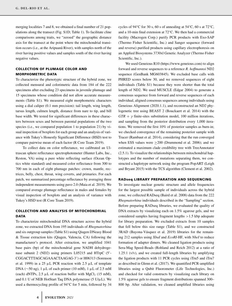
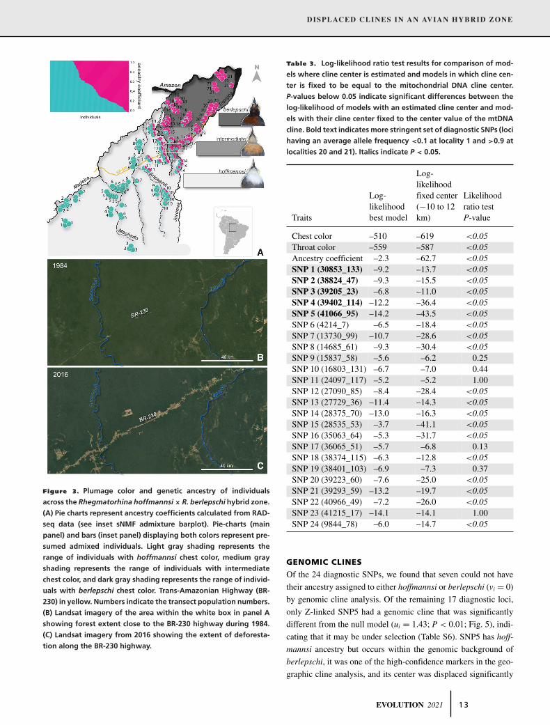
Figure 3. Plumage color and genetic ancestry of individuals

across the Rhegmatorhina hoffmannsi× R. berlepschi hybrid zone.

(A) Pie charts represent ancestry coefficients calculated from RAD-

seq data (see inset sNMF admixture barplot). Pie-charts (main

panel) and bars (inset panel) displaying both colors represent pre-

sumed admixed individuals. Light gray shading represents the

range of individuals with hoffmannsi chest color, medium gray

shading represents the range of individuals with intermediate

chest color, and dark gray shading represents the range of individ-

uals with berlepschi chest color. Trans-Amazonian Highway (BR-

230) in yellow. Numbers indicate the transect population numbers.

(B) Landsat imagery of the area within the white box in panel A

showing forest extent close to the BR-230 highway during 1984.

(C) Landsat imagery from 2016 showing the extent of deforesta-

tion along the BR-230 highway.

Table 3. Log-likelihood ratio test results for comparison of mod-

els where cline center is estimated and models in which cline cen-

ter is fixed to be equal to the mitochondrial DNA cline center.

P-values below 0.05 indicate significant differences between the

log-likelihood of models with an estimated cline center and mod-

els with their cline center fixed to the center value of the mtDNA

cline. Bold text indicatesmore stringent set of diagnostic SNPs (loci

having an average allele frequency <0.1 at locality 1 and >0.9 at

localities 20 and 21). Italics indicate P < 0.05.

Traits

Log-likelihoodbest model

Log-likelihoodfixed center(−10 to 12km)

Likelihoodratio testP-value

Chest color –510 –619 <0.05Throat color –559 –587 <0.05Ancestry coefficient –2.3 –62.7 <0.05SNP 1 (30853_133) –9.2 –13.7 <0.05SNP 2 (38824_47) –9.3 –15.5 <0.05SNP 3 (39205_23) –6.8 –11.0 <0.05SNP 4 (39402_114) –12.2 –36.4 <0.05SNP 5 (41066_95) –14.2 –43.5 <0.05SNP 6 (4214_7) –6.5 –18.4 <0.05SNP 7 (13730_99) –10.7 –28.6 <0.05SNP 8 (14685_61) –9.3 –30.4 <0.05SNP 9 (15837_58) –5.6 –6.2 0.25SNP 10 (16803_131) –6.7 –7.0 0.44SNP 11 (24097_117) –5.2 –5.2 1.00SNP 12 (27090_85) –8.4 –28.4 <0.05SNP 13 (27729_36) –11.4 –14.3 <0.05SNP 14 (28375_70) –13.0 –16.3 <0.05SNP 15 (28535_53) –3.7 –41.1 <0.05SNP 16 (35063_64) –5.3 –31.7 <0.05SNP 17 (36065_51) –5.7 –6.8 0.13SNP 18 (38374_115) –6.3 –12.8 <0.05SNP 19 (38401_103) –6.9 –7.3 0.37SNP 20 (39223_60) –7.6 –25.0 <0.05SNP 21 (39293_59) –13.2 –19.7 <0.05SNP 22 (40966_49) –7.2 –26.0 <0.05SNP 23 (41215_17) –14.1 –14.1 1.00SNP 24 (9844_78) –6.0 –14.7 <0.05

GENOMIC CLINES

Of the 24 diagnostic SNPs, we found that seven could not have

their ancestry assigned to either hoffmannsi or berlepschi (vi = 0)

by genomic cline analysis. Of the remaining 17 diagnostic loci,

only Z-linked SNP5 had a genomic cline that was significantly

different from the null model (ui = 1.43; P < 0.01; Fig. 5), indi-

cating that it may be under selection (Table S6). SNP5 has hoff-

mannsi ancestry but occurs within the genomic background of

berlepschi, it was one of the high-confidence markers in the geo-

graphic cline analysis, and its center was displaced significantly

EVOLUTION 2021 13

G. DEL-RIO ET AL.

Figure 4. Geographic cline analysis. (A) Distance indicates position along the transect, where 0 km is the point that crosses the Aripuanã

River. The cline for the ancestry coefficient is represented by the pink line, for chest color by the orange line, for throat color by the

brown line, for mtDNA by the gray line, and the clines for 15 autosomal SNPs by the green lines. (B) Same as in panel A, except the eight

Z-linked, diagnostic SNPs are represented by blue lines. (C) Boxplots of maximum-likelihood cline center estimates and 95% confidence

intervals, sorted by sizes of cline center confidence intervals. Boxplot colors correspond to cline colors in panels A and B. Asterisks below

horizontal-axis labels indicate cline centers significantly shifted from the cline center estimated for mtDNA. (D) Box plots of maximum-

likelihood cline width estimates and 95% confidence intervals, sorted by sizes of cline width confidence intervals. (E) Geographic position

of cline centers for mtDNA, ancestry coefficient, chest/throat plumage reflectance, and autosomal SNPs along the transect. (F) Geographic

position of cline centers for eight Z-linked, diagnostic SNPs along the transect.

14 EVOLUTION 2021

DISPLACED CLINES IN AN AVIAN HYBRID ZONE

Figure 5. Genomic clines indicate introgression of 15 alleles with hoffmannsi ancestry into the berlepschi genomic background. (A) The

X-axis represents the value of S, which can be interpreted as the probable ancestry of each individual’s genomic background. The Y-axis

represents the logit logistic, where pi is the proportion of copies of locus i inherited from one of the target populations (here berlepschi).

The gray clines represent seven SNPs whose ancestry could not be identified. Blue clines represent two alleles with berlepschi ancestry

introgressed into the hoffmannsi genomic background. Yellow clines and the orange cline represent 15 alleles with hoffmannsi ancestry

introgressed into the berlepschi genomic background. The orange cline represents Z-linked SNP5, the only diagnostic locuswith a genomic

cline significantly different from the null cline, suggesting it may be under selection. (B) v indicates the slope of pi , and u indicates the

relative difference in cline position relative to the inflection point. SNPs with v values equal to zero did not have their ancestry identified

(gray circles), SNPs with negative values of u have berlepschi alleles but are on the genomic background of hoffmannsi (blue circles),

and SNPs with positive u values have hoffmannsi ancestry but are on the genomic background of berlepschi (yellow and orange circles).

The orange circle represents Z-linked SNP5. (C) Plot showing the squared Mahalanobis distance D2 of each SNP, against the expected χ2

distribution. A locus (SNP5, in orange) with D2 greater than expected and visually deviating from quantile-quantile plot is considered an

outlier and could be under selection. Rhegmatorhina illustrations by GDR.

north of the mtDNA cline center, along with several other nuclear

clines.

DEMOGRAPHIC ANALYSIS OF SNP DATA

Estimates of ancestral effective population size were consistent

across G-PhoCS runs with different priors and input datasets (θ̂ =1,600,000 ± 7100 individuals), whereas estimates of divergence

time were more variable (τ̂ = 72,000 ± 11,000 years) (Table S7)

and an order of magnitude younger than previous mitochondrial

estimates of divergence time (Ribas et al. 2018). Model com-

parisons suggested the best fit model: (1) estimated the time of

divergence, as opposed to accepting the divergence time esti-

mated by G-PhoCS or the one presented in Ribas et al. (2018);

(2) included ongoing migration, rather than one single pulse

of migration or an absence of migration; and (3) included uni-

directional migration from berlepschi to hoffmannsi, a pattern

EVOLUTION 2021 15

G. DEL-RIO ET AL.

consistent with hoffmannsi being the invader species over the lo-

cal berlepschi (Currat et al. 2008) (Table S8).

DiscussionThe mitochondrial, nuclear, and plumage color patterns we char-

acterized in Rhegmatorhina suggest that, after secondary con-

tact in the vicinity of the Aripuanã River where the mitochon-

drial transition occurs, the majority of traits and loci experienced

a net northward movement, with most clines currently centered

in a narrow band of habitat between the Sucunduri and Tapa-

jós Rivers. This interpretation is based on significant displace-

ment of the mitochondrial cline from most other clines, including

plumage color, and by the greater net introgression of berlepschi

nuclear alleles into the genomic background of hoffmannsi—the

expected pattern if hoffmannsi is the invader and berlepschi the

invadee (Figs. 3 and 4; Currat et al. 2008). It is possible that the

current geographic position of the nuclear and phenotypic hybrid

zone is stabilized by a habitat bottleneck created by the narrow

forest corridor between the Sucunduri River and the Tapajós and

Juruena Rivers (Fig. 3).

If the hybrid zone is moving northward, one eventual out-

come, barring anthropogenic effects and assuming its position is

not fully stabilized by the geographic bottleneck described above,

would be extinction of berlepschi via genetic swamping. How-

ever, significant habitat degradation in this region is altering the

natural processes operating in the hybrid zone, most significantly

the construction of highway BR-230 during the 1960s and 1970s.

Also known as the Trans-Amazonian Highway, BR-230 bisects

the hybrid zone precisely in the narrow band of habitat where

most nuclear clines are centered and where phenotypic interme-

diates occur (Fig. 3). Until relatively recently, habitable forest

still occurred along the highway in this region that would have al-

lowed antbirds to cross. This is no longer the case. We speculate

that dispersal across BR-230 is now greatly diminished, at best.

Additional data are needed to directly examine the influence of

BR-230 on bird densities and dispersal, as well as on the Eciton

army ants followed by the birds, but it seems clear that the future

of the hybrid zone will now be determined in part by BR-230.

In terms of evolutionary forces, the narrowness of the mi-

tochondrial cline makes it likely that natural selection is playing

a significant role in its maintenance, but we cannot reject neu-

tral diffusion in explaining the wider nuclear clines. Nonetheless,

there is some evidence for reduced hybrid fitness in the nuclear

genome. For example, the disproportionate number of Z-linked

diagnostic SNPs could indicate greater selection against females

(the heterogametic sex in birds) in accordance with Haldane’s

Rule (Carling and Brumfield 2008). Below we examine some

of the major patterns in the Rhegmatorhina hybrid zone, explore

some potential causes of these patterns, and propose hypotheses

to be tested in future work.

DISPLACEMENT OF MITOCHONDRIAL AND NUCLEAR

CLINES

We found that the center of the mitochondrial cline near the

Aripuanã River was displaced significantly from the center of

the clines for plumage color and most nuclear loci (Fig. 4). Em-

pirical examples of hybrid zones in which mitochondrial and

nuclear/phenotypic clines are displaced from one another are

relatively abundant in the literature (summarized in Toews and

Brelsford 2012). One hypothesis for the discordance we can-

not reject is that the mitochondrial gene we sampled (ND2)

evolves too slowly to exhibit sequence divergence between the

two species. It could be that sampling of more rapidly evolving

mitochondrial genes would reveal mitochondrial divergence in

the same geographic location as the SNP and phenotypic tran-

sitions. This would be unusual, because it would imply that the

mitochondrial divergence we observed within hoffmannsi across

the nearby Aripuanã occurred without any accompanying nuclear

or phenotypic divergence. However, the SNP data suggested the

species divergence could have been very recent (70,000 ya), in

which case it would not be unusual to see little, if any, mitochon-

drial divergence. Assuming the displacement is real, three other

hypotheses proposed to explain displaced mitochondrial and nu-

clear geographic clines in vertebrates are genetic drift, adaptive

introgression of mtDNA, and mtDNA of one lineage left behind

following movement of the hybrid zone (Currat et al. 2008).

The genetic drift hypothesis suggests that some proportion

of the among-locus variance in geographic cline centers is due

to sampling error and genetic drift. Both factors certainly ac-

count for a proportion of the among-trait variance we observed

in cline centers and widths. Whether drift alone could account

for the displaced mitochondrial cline is unclear, but it is plausible

given the smaller effective population size of mitochondrial loci

(Nei and Tajima 1981). For example, initial secondary contact be-

tween hoffmannsi and berlepschi could have been at the Sucun-

duri River, the site of the current transition zone between the two

plumage types. Genetic drift in the hybrid zone could have led

to the fixation of the berlepschi haplotype west of the Sucunduri.

We cannot reject this possibility, but it seems less likely given

the essential cytonuclear associations often found in species (Hill

2019).

The adaptive introgression hypothesis proposes that one of

the two mitochondrial haplotypes is selectively advantageous in

both species (Toews et al. 2014). For Rhegmatorhina, this would

suggest the berlepschi mitochondrial haplogroup crossed the nu-

clear hybrid zone and introgressed southward as far as the mi-

tochondrial break near the Aripuanã River. This seems unlikely

based on Haldane’s rule in which reduced hybrid fitness is usually

16 EVOLUTION 2021

DISPLACED CLINES IN AN AVIAN HYBRID ZONE

more pronounced in the heterogametic sex. Because females are

the heterogametic sex in birds, this effect would also limit the in-

trogression of the matrilineally inherited mitochondrion. In terms

of the berlepschi haplotype spreading due to a selective advan-

tage, we have no way to directly measure the fitness of different

mitochondrial haplotypes and thus cannot evaluate this hypothe-

sis. However, there are no obvious thermal or other gradients in

this region that would be a selection gradient. Moreover, studies

that have modeled the expansion of advantageous genes across

hybrid zones show that they spread to fixation extremely rapidly

(Piálek and Barton 1997). If so, then the mitochondrial haplotype

should have spread throughout the distribution of hoffmannsi, but

we only observed it as far as the Aripuanã River. One potential

explanation for its lack of further spread would be if birds are un-

able to circumnavigate the Aripuanã, either due to the river itself

or to inhospitable habitat at its headwaters. This is something we

plan to explore in future work, but the presence of hoffmannsi on

both banks indicates the Aripuanã River was circumnavigable at

some point in the past, which would have provided an opportunity

for an advantageous haplotype to progress. In sum, we cannot re-

ject an adaptive mitochondrial explanation, but it seems unlikely.

More sampling in the headwaters of the Aripuanã is needed, as

are studies of mitochondrial function in the different haplotypes.

In a third hypothesis, the mtDNA of one haplogroup, in our

case hoffmannsi A, failed to accompany the northward-moving

nuclear hybrid zone (Gyllensten and Wilson 1987) leading to dis-

placed mitochondrial and nuclear clines. As with most hybrid

zones, the exact mechanism by which this displacement would

have occurred is unknown but it could be due to an asymmetry

in fitness that results in only one of the two mitochondrial haplo-

types being passed on to hybrids. Differential inheritance of mito-

chondrial haplotypes could occur by prezygotic mechanisms that

result in unidirectional hybridization or by a postzygotic mecha-

nism in which hybridization is reciprocal but the offspring’s via-

bility or fertility is not (Wirtz 1999).

There are no studies addressing the prevalence of prezy-

gotic barriers in Rhegmatorhina. Because many aspects of the

biology of hoffmannsi and berlepschi, with the exception of

plumage color, are essentially indistinguishable between the two

species (Willis 1969), plumage color would be the putative fac-

tor influencing assortative mating. Instead of a strong prezy-

gotic barrier, our results could indicate a skewed preference for

individuals with white plumage. For example, in lekking Mana-

cus manakins, skewed mating success of yellow males may re-

sult in a bias toward hybridization between females of the white

species (White-collared Manakins, Manacus candei) and males

of the Golden-collared Manakins (Manacus vitellinus) at leks in

western Panama (Stein and Uy 2006). In Rhegmatorhina, if mat-

ings with individuals having white plumage are more frequent

than with individuals having a black throat and brown chest,

it is expected that the white plumage of hoffmannsi would be-

come more prevalent, supplanting dark individuals in the origi-

nal range of berlepschi. Alternatively, the northward advance of

white plumage could reflect genetic dominance of the alleles re-

sponsible for the white phenotype over the alleles promoting the

alternative plumage colors (Semenov et al. 2021). This idea could

be tested if the loci and alleles responsible for plumage color

were known. Although preference for the white plumage and

dominance could explain a northward movement of hoffmannsi

white plumage color, the two mechanisms fail to explain why the

hoffmannsi mitochondrial haplotype would not “accompany” the

plumage color movement.

Mechanisms also exist that would produce, in the early

stages of secondary contact, offspring that only have one of the

two mitochondria represented, but it is difficult to envision this

pattern persisting into later generations. For example, if initial

secondary contact was restricted to a few hoffmannsi males that

circumnavigated the Aripuanã into the distribution of berlepschi,

then all hybrids, at least initially, would have the berlepschi hap-

lotype. The problem is that this scenario of berlepschi haplotypes

in hybrid offspring would break down when female hoffmannsi

eventually circumnavigated the river and hybridized with berlep-

schi. The hypothesis also seems less likely because female birds

generally tend to disperse greater distances than males (Green-

wood 1980). If anything, it would be hoffmannsi females that

first colonized the east bank of the Aripuanã. This would have

resulted in the hoffmannsi A haplogroup on the east bank of the

Aripuanã. Low levels of movement across the Aripuanã are pos-

sible. To date, we have observed three hoffmannsi A individuals

on the right bank of the Aripuanã (two females and one male), all

at its narrow headwaters (Fig. 2).

A postzygotic mechanism, and a cytonuclear incompatibil-

ity in particular, seems like a plausible hypothesis to explain the

displaced clines we observed in Rhegmatorhina. Empirical stud-

ies of avian hybridization have demonstrated negative, female-

biased fitness effects such as inviability and infertility, in accor-

dance with Haldane’s rule (Carling and Brumfield 2008; Gowen

et al. 2014). Detrimental fitness effects experienced by females

extend to the mitochondrial genome, as well as to any nuclear

genes that are linked epistatically to the mitochondrion. In Rheg-

matorhina, the discordance we observed could be explained if

females are inviable or infertile when they have the berlepschi

mitochondrial haplogroup and an unknown Z-linked or autoso-

mal hoffmannsi allele(s) (Dasmahapatra et al. 2002; Mishmar

et al. 2003). If the fitness reductions were only partial inviabil-

ity or partial infertility, then the mitochondrial cline we observed

would not have been so narrow. We predict that the unknown hoff-

mannsi nuclear allele(s) should also have its cline centered near

the Aripuanã River. Among the diagnostic SNPs we identified,

the geographic clines of several are statistically concordant with

EVOLUTION 2021 17

G. DEL-RIO ET AL.

the mtDNA cline, yet their cline widths are much wider than the

mtDNA cline, suggesting these nuclear loci are not involved di-

rectly in mitonuclear incompatibilities (Fig. 4C, D). The details

of a putative cytonuclear interaction are currently unknown to us,

but they are the subject of ongoing work.

MOVING HYBRID ZONE

After secondary contact, which we assume occurred somewhere

in the vicinity of the Aripuanã River, the plumage traits and nu-

clear loci, excepting any nuclear gene(s) involved in a putative

cytonuclear interaction, moved northward to their current posi-

tions in the narrow band of habitat between the Sucunduri River

and the Tapajós/Juruena Rivers (Fig. 3). Viewed from the per-

spective of a biological invasion with hybridization and assum-

ing hoffmannsi is the invader and berlepschi the invadee, the ge-

ographic structuring of genetic variation, including the unidirec-

tional migration from berlepschi to hoffmannsi indicated by the

SFS, is consistent with expectations (Currat et al. 2008): a greater

geographic extent of berlepschi introgression into hoffmannsi

(Fig. 3). Alternatively, the berlepschi nuclear alleles found be-

tween the Aripuanã and Sucunduri Rivers could be interpreted

as a genetic wake left behind the northward-moving hybrid zone

(Rohwer et al. 2001) or they could be viewed as ancestral alleles

that have been retained. The retention hypothesis seems unlikely

given the decay of berlepschi alleles moving southward from the

hybrid zone, but the genetic wake hypothesis is a plausible ex-

planation for the presence of some alleles. Finally, there may be

a more complicated history of hybridization that is difficult to

disentangle from extant patterns of diversity (Wang et al. 2019).

The ideal corroborating data to support a moving hybrid

zone would be direct observations of historical specimens in pu-

tative invaded areas. For example, Wang et al. (2019) used sam-

ples collected 30 years apart to assess hybrid zone movements

in the Setophaga occidentalis/townsendi hybrid zone. Unfortu-

nately, there are no census data or specimens from the Rheg-

matorhina hybrid zone that we could use to directly assess past

movements. Seven individuals of parental hoffmannsi collected

in 1971 from the east bank of the Aripuanã are some of the very

few historical specimens from the region (MZUSP 62285, 62286,

62287, 62288, 62293, 62294, and 62295), and these are consis-

tent with the modern phenotypic structure of the hybrid zone.

The Aripuanã River is well known as a site of taxon turnover

(Cohn-Haft et al. 2007), and mitochondrial studies that exam-

ined the phylogeographic structure of understory birds in this re-

gion have all found mitochondrial breaks of varying ages between

populations from its opposite banks, including in Glyphorynchus

spirurus (Fernandes et al. 2013), Thamnophilus aethiops (Thom

and Aleixo 2015), Hypocnemis rondoni (Fernandes et al. 2014),

and Lepidothrix nattereri (Dias et al. 2018). Several avian taxon

pairs also turnover across the Sucunduri River (Fernandes 2013;

Whitney et al. 2013; Schultz et al. 2019), but the Rhegmatorhina

hybrid zone is the only one of these turnovers that has been

analyzed. The occurrence of multiple contact zones within the

Madeira/Tapajós interfluve suggests a dynamic system that pro-

vides a natural laboratory to study the outcomes of secondary

contact.

AUTHOR CONTRIBUTIONSGDR, MAR, BMW, FS, LFS, BCF, and RTB conceived the study andwrote the manuscript. GDR, MAR, BMW, FS, and LFS performed fieldwork from 2004 to 2019. GDR collected laboratory data. GDR collectedmuseum specimen data. GDR and BCF conducted analyses. GDR madefigures.

ACKNOWLEDGMENTSThe authors thank the editors B. Emerson and A. McAdam and twoanonymous referees for their comments and suggestions, all of whichimproved this manuscript. The authors thank C. Ribas, M. Cohn-haft,G. Lima (INPA), A. Aleixo, F. Lima (MPEG), S. Hackett, J. Bates, andB. Marks (FMNH), D. Dittmann (LSU), and C. Miyaki (University ofSão Paulo) for providing valuable loans of tissues and for opening thedoors of their bird collections and laboratories to GDR. The authors arethankful for all the volunteers that helped with Rhegmatorhina fieldworkover the course of more than nine LSU-MZUSP expeditions, and the au-thors are especially grateful to D. Schmitt, G. Schmitt, T. Jackson, M.Lima, P. Balduíno, M. Félix, I. Jean and F. Arantes. The authors thankE. Duval and the Manakin Genomics Research Coordination Network(DBI-1457541) for making the Chiroxiphia genome assembly availablethrough NCBI. The authors thank J. Salter, C. Oliveros, A. Schoonmaker,R. Beco, F. Bocalini, S. Bolívar, and J. Battilana for helping with labo-ratory work. The authors thank B. Fitzpatrick for insightful discussionsabout genomic clines. The authors thank I. Gronau, M. Hickerson, andY. Song for discussions about demographic inference and introgressiondirection. F. Alda, G. Bravo and R. Marcondes provided helpful com-ments on an earlier version of the manuscript. Portions of this researchwere conducted with high-performance computing resources providedby Louisiana State University (http://www.hpc.lsu.edu) and LouisianaOptical Network Infrastructure (http://www.loni.org). Financial supportwas provided by the National Science Foundation (DEB-1146265, DEB-1655624), Coypu Foundation, CNPq (2014/2009-1), American Asso-ciation of University Women, AMNH Chapman Memorial Fund, LSUAlumni Association, startup funds from LSU to BCF, Society of System-atic Biologists, Scientific Exploration Society, and Wilson OrnithologicalSociety.

DATA ARCHIVINGRaw read data used for genome assembly are available from Na-tional Center for Biotechnology Information (NCBI) BioProject PR-JNA545868. This Whole Genome Shotgun project has been deposited atDDBJ/ENA/GenBank under the accession VZSN00000000, and the ver-sion described in this article (the RaGOO pseudo-chromosomal assem-bly) is VZSN02000000 (NCBI PRJNA669390). RAD sequencing dataand ND2 sequences are available from BioProject PRJNA763942.

CONFLICT OF INTERESTThe authors declare no conflict of interest.

18 EVOLUTION 2021

DISPLACED CLINES IN AN AVIAN HYBRID ZONE

LITERATURE CITEDAlonge, M., S. Soyk, S. Ramakrishnan, X. Wang, S. Goodwin, F. J.

Sedlazeck, Z. B. Lippman, and M. C. Schatz. 2019. Fast and accuratereference-guided scaffolding of draft genomes. Genome Biol. 20:1–17.

Altschul, S. F., W. Gish, W. Miller, E. W. Myers, and D. J. Lipman. 1990.Basic Local Alignment Search Tool 2. J. Mol. Biol. 215:403–410.

Backenroth, D., and S. Carmi. 2019. A test for deviations from expected geno-type frequencies on the X chromosome for sex-biased admixed popula-tions. Heredity 123:470–478.

Baird, N. A., P. D. Etter, T. S. Atwood, M. C. Currey, A. L. Shiver, Z. A.Lewis, E. U. Selker, W. A. Cresko, and E. A. Johnson. 2008. RapidSNP discovery and genetic mapping using sequenced RAD markers.PLoS ONE 3:1–7.

Barton, N. H. 2008. The effect of a barrier to gene flow on patterns of geo-graphic variation. Genet. Res. 90:139–149.

Barton, N. H., and K. S. Gale. 1993. Genetic analysis of hybrid zones. Pp.13–45 in R. G. Harrison, ed. Hybrid zones and the evolutionary process.Oxford Univ. Press, New York.

Bayona-Vásquez, N. J., T. C. Glenn, T. J. Kieran, T. W. Pierson, S. L.Hoffberg, P. A. Scott, K. E. Bentley, J. W. Finger, S. Louha, N.Troendle, et al. 2019. Adapterama III: quadruple-indexed, double/triple-enzyme RADseq libraries (2RAD/3RAD). PeerJ 2019:1–25.

Bazykin, A. D. 1969. Hypothetical mechanism of speciation. Evolution23:685–687.

Bocalini, F., S. D. Bolívar-Leguizamón, L. F. Silveira, and G. A. Bravo.2021. Comparative phylogeographic and demographic analyses reveala congruent pattern of sister relationships between bird populations ofthe northern and south-central Atlantic Forest. Mol. Phylogenet. Evol.154:106973.

Bolger, A. M., M. Lohse, and B. Usadel. 2014. Trimmomatic: a flexible trim-mer for Illumina sequence data. Bioinformatics 30:2114–2120.

Bouckaert, R., J. Heled, D. Kuhnert, T. Vaughan, C.-H. Wu, D. Xie, M. A.Suchard, A. Rambaut, and A. J. Drummond. 2014. BEAST2: a soft-ware platform for Bayesian evolutionary analysis. PLoS Comput. Biol.10:e1003537.

Bronson, C. L., T. C. Grubb, G. D. Sattler, and M. J. Braun. 2005. Repro-ductive success across the Black-capped Chickadee (Poecile atricapil-lus) and Carolina Chickadee (P. carolinensis) hybrid zone in Ohio. Auk122:759–772.

Burnham, K. P., and D. R. Anderson. 2002. Model selection and multimodelinference: a practical information-theoretic approach. Springer, NewYork.

Butlin, R. K., and C. M. Smadja. 2018. Coupling, reinforcement, and specia-tion. Am. Nat. 191:155–172.

Carling, M. D., and R. T. Brumfield. 2008. Haldane’s rule in an avian system:using cline theory and divergence population genetics to test for dif-ferential introgression of mitochondrial, autosomal, and sex-linked lociacross the Passerina bunting hybrid zone. Evolution 62:2600–2615.

Catchen, J., P. A. Hohenlohe, S. Bassham, A. Amores, and W. A. Cresko.2013. Stacks: an analysis tool set for population genomics. Mol. Ecol.22:3124–3140.

Chang, C. C., C. C. Chow, L. C. A. M. Tellier, S. Vattikuti, S. M. Purcell,and J. J. Lee. 2015. Second-generation PLINK: rising to the challengeof larger and richer datasets. Gigascience 4:1–16.

Chattopadhyay, B., K. M. Garg, and U. Ramakrishnan. 2014. Effect of di-versity and missing data on genetic assignment with RAD-seq markers.BMC Res. Notes 7:4–6.

Chen, B., J. W. Cole, and C. Grond-Ginsbach. 2017. Departure from Hardy-Weinberg Equilibrium and genotyping error. Front. Genet. 8:1–6.

Clement, M., Q. Snell, P. Walke, D. Posada, and K. Crandall. 2002. TCS: esti-mating gene genealogies. P. 184 in Proceedings of the 16th International

Symposium on Parallel and Distributed Processing. IEEE, Piscataway,NJ.

Cohn-Haft, M., A. M. F. Pacheco, C. L. Bechtoldt, M. F. N. M. Torres, A.M. Fernandes, C. H. Sardelli, and I. T. Macêdo. 2007. Inventário or-nitológico. Pp. 145–178 in D. Rapp Py, ed. Biodiversidade do MédioMadeira: base científicas para propostas de conservação. INPA, Man-aus, Brazil.

Cronemberger, Á., A. Aleixo, E. Mikkelsen, and J. Weir. 2020. Postzygoticisolation drives genomic speciation between highly cryptic Hypocnemis

antbirds from Amazonia. Evolution 5:1689–1699.Currat, M., M. Ruedi, R. J. Petit, and L. Excoffier. 2008. The hidden side

of invasions: massive introgression by local genes. Evolution 62:1908–1920.

Danecek, P., A. Auton, G. Abecasis, C. A. Albers, E. Banks, M. A. DePristo,R. E. Handsaker, G. Lunter, G. T. Marth, S. T. Sherry, et al. 2011. Thevariant call format and VCFtools. Bioinformatics 27:2156–2158.

Dasmahapatra, K. K., M. J. Blum, A. Aiello, S. Hackwel, N. Davies, E. P.Bermingham, and J. Mallet. 2002. Inferences from a rapidly movinghybrid zone. Evolution 56:741–753.

Derryberry, E. P., G. E. Derryberry, J. M. Maley, and R. T. Brumfield. 2014.HZAR: hybrid zone analysis using an R software package. Mol. Ecol.Resour. 14:652–663.

Dias, C., K. de A Lima, J. Araripe, A. Aleixo, M. Vallinoto, I. Sampaio, H.Schneider, and P. S. do Rêgo. 2018. Mitochondrial introgression ob-scures phylogenetic relationships among manakins of the genus Lepi-dothrix (Aves: Pipridae). Mol. Phylogenet. Evol. 126:314–320.

Drummond, A. J., S. Y. W. Ho, M. J. Phillips, and A. Rambaut. 2006. Relaxedphylogenetics and dating with confidence. PLoS Biol. 4:699–710.

Edgar, R. C. 2004. MUSCLE: multiple sequence alignment with high accu-racy and high throughput. Nucleic Acids Res. 32:1792–1797.

Endler, J. A. 1977. Geographic variation, speciation and clines. PrincetonUniv. Press, Princeton, NJ.

Feng, S., J. Stiller, Y. Den, J. Armstrong, Q. Fang, A. H. Reeve, D. Xie, G.Chen, C. Guo, B. C. Faircloth, et al. 2020. et al. Dense sampling of birddiversity increases power of comparative genomics. Nature 587:252–257.

Fernandes, A. M. 2013. Fine-scale endemism of Amazonian birds in a threat-ened landscape. Biodivers. Conserv. 22:2683–2694.

Fernandes, A. M., J. Gonzalez, M. Wink, and A. Aleixo. 2013. Multilo-cus phylogeography of the Wedge-billed Woodcreeper Glyphorynchusspirurus (Aves, Furnariidae) in lowland Amazonia: widespread crypticdiversity and paraphyly reveal a complex diversification pattern. Mol.Phylogenet. Evol. 66:270–282.

Fernandes, A. M., M. Wink, C. H. Sardelli, and A. Aleixo. 2014. Multiplespeciation across the Andes and throughout Amazonia: the case of theSpot-backed Antbird species complex (Hylophylax naevius/Hylophylaxnaevioides). J. Biogeogr. 41:1094–1104.

Fitzpatrick, B. M. 2012. Estimating ancestry and heterozygosity of hybridsusing molecular markers. BMC Evol. Biol. 12:1–14.

———. 2013a. HIest: hybird index estimation. R package version 2.0.———. 2013b. Alternative forms for genomic clines. Ecol. Evol. 3:1951–

1966.Frichot, E., F. Mathieu, T. Trouillon, G. Bouchard, and O. François. 2014. Fast

and efficient estimation of individual ancestry coefficients. Genetics196:973–983.

Gay, L., P. A. Crochet, D. A. Bell, and T. Lenormand. 2008. Comparing clineson molecular and phenotypic traits in hybrid zones: a window on tensionzone models. Evolution 62:2789–2806.

Ghurye, J., M. Pop, S. Koren, D. Bickhart, and C. S. Chin. 2017. Scaffoldingof long read assemblies using long range contact information. BMCGenomics 18:1–11.

EVOLUTION 2021 19

G. DEL-RIO ET AL.

Gill, P. E., and W. Murray. 1974. Newton-type methods for unconstrained andlinearly constrained optimization. Math. Program. 7:311–350.

Glenn, T. C., N. J. Bayona-Vasquez, T. J. Kieran, T. W. Pierson, S. L.Hoffberg, P. A. Scott, K. E. Bentley, J. W. Finger, P. R. Watson, S.Louha, et al. 2017. Adapterama III: quadruple-indexed, triple-enzymeRADseq libraries for about $1USD per Sample (3RAD). bioRxivhttps://doi.org/10.1101/205799.

Gompert, Z., and C. A. Buerkle. 2010. Introgress: a software packagefor mapping components of isolation in hybrids. Mol. Ecol. Resour.10:378–384.

———. 2011. Bayesian estimation of genomic clines. Mol. Ecol. 20:2111–2127.

———. 2016. What, if anything, are hybrids: enduring truths and challengesassociated with population structure and gene flow. Evol. Appl. 9:909–923.

Gompert, Z., T. L. Parchman, and C. A. Buerkle. 2012. Genomics of isolationin hybrids. Philos. Trans. R. Soc. B Biol. Sci. 367:439–450.

Gowen, F. C., J. M. Maley, C. Cicero, A. T. Peterson, B. C. Faircloth, T. C.Warr, and J. E. McCormack. 2014. Speciation in Western Scrub-Jays,Haldane’s rule, and genetic clines in secondary contact. BMC Evol.Biol. 14:1–15.

Greenwood, P. J. 1980. Mating systems, philopatry and dispersal in birds andmammals. Anim. Behav. 28:1140–1162.

Gronau, I., M. J. Hubisz, B. Gulko, C. G. Danko, and A. Siepel. 2011.Bayesian inference of ancient human demography from individualgenome sequences. Nat. Genet. 43:1031–1035.

Gyllensten, U., and A. C. Wilson. 1987. Interspecific mitochondrial DNAtransfer and the colonization of Scandinavia by mice. Genet. Res.49:25–29.

Harrison, R. G. 1993. Hybrid zones and the evolutionary process. OxfordUniv. Press, Ithaca, NY.

Hewitt, G. M. 1988. Hybrid Zones - natural laboratories for evolutionary stud-ies. Trends Ecol. Evol. 3:158–167.

Hill, G. E. 2019. Mitonuclear ecology. Oxford Univ. Press, Oxford, U.K.Johnson, E. I., and J. D. Wolfe. 2018. Molt in Neotropical birds: life history

and aging criteria. 51st ed. American Ornithological Society CRC Press,Boca Raton, FL.

Johnson, R., and D. W. Wichern. 1998. Applied multivariate statistical analy-sis. Prentice Hall, Englewood Cliffs, NJ.

Jombart, T., and I. Ahmed. 2011. adegenet 1.3-1: new tools for the analysisof genome-wide SNP data. Bioinformatics 27:3070–3071.

Kamm, J., J. Terhorst, R. Durbin, and Y. S. Song. 2020. Efficiently inferringthe demographic history of many populations with allele count data. J.Am. Stat. Assoc. 115:1472–1487.

Kawakami, T., R. K. Butlin, M. Adams, D. J. Paull, J. B. Steven, D. J. Paull,R. K. Butlin, and M. Adams. 2009. Genetic analysis of a chromosomalhybrid zone in the Australian Morabine grasshoppers (Vandiemenella

viatica species group). Evolution 63:139–152.Leigh, J. W., and D. Bryant. 2015. PopART: full-feature software for haplo-

type network construction. Methods Ecol. Evol. 6:1110–1116.Li, H. 2013. Aligning sequence reads, clone sequences and assembly contigs

with BWA-MEM. arXiv:1303.3997v2.Linck, E., and C. J. Battey. 2019. Minor allele frequency thresholds strongly

affect population structure inference with genomic data sets. Mol. Ecol.Resour. 19:639–647.

Liu, Y., J. Schröder, and B. Schmidt. 2013. Musket: a multistage k-mer spectrum-based error corrector for Illumina sequence data.Bioinformatics 29:308–315.

Maia, R., H. Gruson, J. A. Endler, and T. E. White. 2019. pavo 2.0: new toolsfor the spectral and spatial analysis of colour in R. Methods Ecol. Evol.10:1097–1107.

McEntee, J. P., J. G. Burleigh, and S. Singhal. 2020. Dispersal predicts hybridzone widths across animal diversity: implications for species bordersunder incomplete reproductive isolation. Am. Nat. 196:9–28.

Mishmar, D., E. Ruiz-Pesini, P. Golik, V. Macaulay, A. G. Clark, S. Hosseini,M. Brandon, K. Easleyf, E. Chen, M. D. Brown, et al. 2003. Natural se-lection shaped regional mtDNA variation in humans. Proc. Natl. Acad.Sci. USA 100:171–176.

Nadachowska-Brzyska, K., C. Li, L. Smeds, G. Zhang, and H. Ellegren. 2015.Temporal dynamics of avian populations during pleistocene revealed bywhole-genome sequences. Curr. Biol. 25:1375–1380.

Nei, M., and F. Tajima. 1981. Genetic drift and estimation of effective popu-lation size. Genetics 98:625–640.

Nurk, S., A. Bankevich, D. Antipov, A. Gurevich, A. Korobeynikov, A.Lapidus, A. Prjibelsky, A. Pyshkin, A. Sirotkin, Y. Sirotkin, et al. 2013.Assembling genomes and mini-metagenomes from highly chimericreads. Pp. 158–170 in M. Deng, R. Jiang, F. Sun, and X. Zhang, eds.Research in computational molecular biology. RECOMB 2013. Lecturenotes in computer science. Vol. 7821. Springer, Berlin.

Oswald, J. A., I. Overcast, W. M. Mauck, M. J. Andersen, and B. T. Smith.2017. Isolation with asymmetric gene flow during the nonsynchronousdivergence of dry forest birds. Mol. Ecol. 26:1386–1400.

Phillips, B. L., S. J. E. Baird, and C. Moritz. 2004. When vicars meet: a nar-row contact zone between morphologically cryptic phylogeographic lin-eages of the rainforest skink, Carlia rubrigularis. Evolution 58:1536–1548.

Piálek, J., and N. H. Barton. 1997. The spread of an advantageous allele acrossa barrier: the effects of random drift and selection against heterozygotes.Genetics 145:493–504.

Pulido-Santacruz, P., A. Aleixo, and J. T. Weir. 2018. Morphologically crypticAmazonian bird species pairs exhibit strong postzygotic reproductiveisolation. Proc. R. Soc. Lond. Biol. Sci. 285:20172081.

Python Software Foundation. 2021. Python language reference. Python Soft-ware Foundation, Wilmington, DE.

R Core Team. 2019. R: a language and environment for statistical computing.R Foundation for Statistical Computing, Vienna.

Rambaut, A., M. A. Suchard, D. Xie, and A. J. Drummond. 2014. Tracer v1.6.Rhie, A., S. A. Mccarthy, O. Fedrigo, J. Damas, G. Formenti, S. E. London,

D. F. Clayton, C. V. Mello, and S. R. Friedrich. 2021. Towards com-plete and error-free genome assemblies of all vertebrate species. Nature592:737–746.

Ribas, C. C., A. Aleixo, C. Gubili, F. M. d’Horta, R. T. Brumfield, andJ. Cracraft. 2018. Biogeography and diversification of Rhegmatorhina

(Aves: Thamnophilidae): implications for the recent evolution of Ama-zonian landscapes. J. Biogeogr. 45:917–928.

Rohland, N., and D. Reich. 2012. Cost-effective, high-throughput DNA se-quencing libraries for multiplexed target capture. Genome Res. 22:939–946.

Rohwer, S., E. Bermingham, and C. Wood. 2001. Plumage and mitochon-drial DNA haplotype variation across a moving hybrid zone. Evolution55:405–422.

Sahlin, K., F. Vezzi, B. Nystedt, J. Lundeberg, and L. Arvestad. 2014. BESST- efficient scaffolding of large fragmented assemblies. BMC Bioinfor-matics 15:281.

Schultz, E. D., J. Pérez-Emán, A. Aleixo, C. Y. Miyaki, R. T. Brumfield,J. Cracraft, and C. C. Ribas. 2019. Diversification history in the Den-

drocincla fuliginosa complex (Aves: Dendrocolaptidae): insights frombroad geographic sampling. Mol. Phylogenet. Evol. 140:106581.

Semenov, G. A., E. Linck, E. D. Enbody, R. B. Harris, D. R. Khaydarov, P.Alström, L. Andersson, and S. A. Taylor. 2021. Asymmetric introgres-sion reveals the genetic architecture of a plumage trait. Nat. Commun.12:1–9.

20 EVOLUTION 2021

DISPLACED CLINES IN AN AVIAN HYBRID ZONE

Shafer, A. B. A., C. R. Peart, S. Tusso, I. Maayan, A. Brelsford, C. W. Wheat,and J. B. W. Wolf. 2017. Bioinformatic processing of RAD-seq data dra-matically impacts downstream population genetic inference. MethodsEcol. Evol. 8:907–917.

Smith, B. T., M. G. Harvey, B. C. Faircloth, T. C. Glenn, and R. T. Brumfield.2014. Target capture and massively parallel sequencing of ultracon-served elements for comparative studies at shallow evolutionary timescales. Syst. Biol. 63:83–95.

Sorenson, M. D., J. C. Ast, D. E. Dimcheff, T. Yuri, and D. P. Mindell. 1999.Primers for PCR-based approach to mitochondrial genome sequencingin birds and other vertebrates. Mol. Phylogenet. Evol. 12:105–114.

Stein, A. C., and J. A. C. Uy. 2006. Unidirectional Introgression of a sexuallyselected trait across an avian hybrid zone: a role for female choice?Evolution 60:1476.

Szymura, J. M., and N. H. Barton. 1986. Genetic analysis of a hybrid zonebetween the Fire-Bellied Toads, Bombina bombina and B. variegata,near Cracow in southern Poland. Evolution 40:1141–1159.

Thom, G., and A. Aleixo. 2015. Cryptic speciation in the white-shoulderedantshrike (Thamnophilus aethiops, Aves - Thamnophilidae): the tale ofa transcontinental radiation across rivers in lowland Amazonia and thenortheastern Atlantic Forest. Mol. Phylogenet. Evol. 82:95–110.

Thom, G., A. T. Xue, A. O. Sawakuchi, C. C. Ribas, M. J. Hickerson, A.Aleixo, and C. Miyaki. 2020. Quaternary climate changes as speciationdrivers in the Amazon floodplains. Sci. Adv. 6:eaax4718.

Toews, D. P., and A. Brelsford. 2012. The biogeography of mitochondrial andnuclear discordance in animals. Mol. Ecol. 21:3907–3930.

Toews, D. P. L., A. Brelsford, and D. E. Irwin. 2014. Isotopic variation acrossthe Audubon’s-myrtle warbler hybrid zone. J. Evol. Biol. 27:1179–1191.

Wang, M. S., M. Thakur, M. S. Peng, Y. Jiang, L. A. F. Frantz, M. Li, J.J. Zhang, S. Wang, J. Peters, N. O. Otecko, et al. 2020. 863 Genomesreveal the origin and domestication of chicken. Cell Res. 30:693–701.

Wang, S., S. Rohwer, K. Delmore, and D. E. Irwin. 2019. Cross-decades sta-bility of an avian hybrid zone. J. Evol. Biol. 32:1242–1251.

Whitney, B. M., F. Schunck, M. A. Rêgo, and L. F. Silveira. 2013. A newspecies of flycatcher in the Tolmomyias assimilis radiation from thelower Sucunduri-Tapajós interfluvium in central Amazonian Brazil her-alds a new chapter in Amazonian biogeography. Pp. 297–300 in J. delHoyo, A. Elliott, J. Sargatal, and D. A. Christie, eds. Handbook of thebirds of the world. Lynx Edicions, Barcelona, Spain.

Wigginton, J. E., D. J. Cutler, and G. R. Abecasis. 2005. A note on exact testsof Hardy-Weinberg Equilibrium. Am. J. Hum. Genet. 76:887–893.

Willis, E. O. 1969. On the behavior of five species of Rhegmatorhina, ant-following antbirds of the Amazon basin. Wilson Bull. 81:363–395.

Wirtz, P. 1999. Mother species-father species: unidirectional hybridization inanimals with female choice. Anim. Behav. 58:1–12.

Woltmann, S., R. S. Terril, M. J. Miller, and M. L. Brady. 2010. Chestnut-backed Antbird (Poliocrania exsul) version 1.0. In T. S. Schulenberg,ed. Birds of the world. Cornell Lab of Ornithology, Ithaca, NY.

Associate Editor: B. EmersonHandling Editor: A. G. McAdam

Supporting InformationAdditional supporting information may be found online in the Supporting Information section at the end of the article.

EVOLUTION 2021 21