Testing Uncovered Interest Rate Parity Using LIBOR

Muhammad Omer Jakob de Haan Bert Scholtens

CESIFO WORKING PAPER NO. 3839 CATEGORY 7: MONETARY POLICY AND INTERNATIONAL FINANCE

JUNE 2012

An electronic version of the paper may be downloaded • from the SSRN website: www.SSRN.com • from the RePEc website: www.RePEc.org

• from the CESifo website: Twww.CESifo-group.org/wp T

CESifo Working Paper No. 3839

Testing Uncovered Interest Rate Parity Using LIBOR

Abstract We test Uncovered Interest Parity (UIP) using LIBOR interest rates for a wide range of maturities. In contrast to other markets, LIBOR markets have minimal frictions which could lead to rejecting UIP. Using panel unit root test suggested by Palm, Smeekes, and Urbain (2010) and cointegration techniques by Westerlund (2007), we find that UIP holds for short-term maturities, when market-specific heterogeneity is controlled for. Furthermore, the estimation results show that the speed of adjustment to the long-run equilibrium is proportional to the maturity of the underlying instrument.

JEL-Code: G120, G150, F310.

Keywords: UIP, LIBOR, panel cointegration.

Muhammad Omer

Faculty of Economics and Business University of Groningen

Groningen / The Netherlands m.omer@rug.nl

Jakob de Haan

Faculty of Economics and Business University of Groningen

Groningen / The Netherlands jakob.de.haan@rug.nl

Bert Scholtens

Faculty of Economics and Business University of Groningen

Groningen / The Netherlands l.j.r.scholtens@rug.nl

We like to thank Jean-Pierre Urbain and Jan Jacobs for their guidance and comments. The views expressed do not necessarily reflect the views of De Nederlandsche Bank.

2

1. Introduction Uncovered Interest Rate Parity (henceforth UIP) is one of the most researched topics in

international economics. According to the UIP hypothesis, the difference in the return on

identical assets from two different countries should be fully offset by the differential of

the spot and the expected future exchange rate at the points in time when the interest-

bearing assets are bought and redeemed. For the short-term horizon, UIP is rejected due

to frictions, like irrational expectations (Mark and Wu, 1998; Frankel and Froot, 1989;

Carlson and Osler, 1999), forecast errors (Lewis, 1989; 1995) and/or non-linearities

(Sarno, Valente and Leon, 2006; Baillie and Kilic, 2006; Flood and Rose, 1996; Flood

and Taylor, 1996 and Bansal and Dahlquist, 2000). Numerous studies examine the

importance of these frictions.1 However, to date no study addresses whether UIP holds if

frictions are minimal. We examine this issue using London Interbank Offered Rates

(LIBOR). LIBOR is a daily reference rate based on the interest rates paid on unsecured

interbank deposits by international banks. As will be explained in some detail in section

2, the LIBOR market provides an environment with minimal economic frictions that may

lead to rejection of UIP.

Our paper contributes to the literature in the following ways. First, to the best of

our knowledge LIBOR has never been directly used for testing UIP although Juselius and

MacDonald (2004), Harvey (2005) and Ichiue and Koyama (2007) have used LIBOR, but

only as a proxy for Japanese domestic interest rates. Interestingly, LIBOR is a widely

used benchmark for global financial transactions and provides a setup where several of

the known frictions responsible for the failure of UIP are absent.

Second, this study tests UIP using fourteen different maturities, ranging from one

week to 12-months. Previous studies on UIP mostly used only two or three maturities,

such as 3-months, 6-months, or sometimes 12-months, generalizing the findings. The use

of several maturities helps us to identify when UIP holds.

Third, we employ panel unit root and cointegration techniques. The UIP literature

has extensively adopted unit root and cointegration techniques. However, the use of panel

cointegration is relatively new to this area. A panel setup has several advantages. In the

1 Reviews can be found in Froot and Thaler (1990), MacDonald and Taylor (1992), Flood and Taylor (1996), Isard (1996), Pasricha (2006), and Alper, Ardic, and Fendoglu (2009).

3

first place, it takes into account that financial markets are not isolated. For instance, a

shock to the US debt market that increases US interest rates vis-à-vis Japanese interest

rates will activate carry trade which, in turn, may affect the US Dollar/ Japanese Yen

exchange rate. However, the US specific interest rate shock also affects other markets.

Panel techniques exploit the multi-currency environment to isolate individual currency-

specific effects. The within transformation, used to isolate the currency specific effect,

may lower the correlation between the series, hence a panel set-up helps in mitigating the

multicollinearity problem. Moreover, a panel approach yields efficiency gains and

enhances the possibility of estimating the complex dynamics. Finally, the increased

sample size is expected to improve the power of the tests.

Following most previous studies, we assume perfect foresight with respect to

exchange rates. However, our findings deviate from the conclusions reached in most

previous UIP studies. First, we conclude that UIP holds for almost all maturities between

7 and 12 months. Furthermore, the speed of adjustment of the exchange rate due to a

shock in the interest rates is related to the maturity of the underlying assets, which is not

in line with the efficient market hypothesis.

The remainder of the paper is structured as follow. Section 2 discusses the market

structure of LIBOR. Section 3 reviews some previous studies, while section 4 delves into

data and methodology issues. Section 5 presents our results. Finally, section 6 offers our

conclusions.

2. Market homogeneity and LIBOR London Inter-Bank Offered Rates (LIBOR) is a widely used benchmark for national and

international transactions. Forbes Investopedia estimates that $360 trillion worth of

international financial products are benchmarked with LIBOR. Additionally, one trillion

dollars of sub-prime mortgages have rates adjustable to LIBOR.2 LIBOR rates are used in

LIBOR market Model (LMM) to produce the LIBOR forward rates.3 These LIBOR

forward rates are essential for pricing financial derivatives and determining a hedging 2 http://www.investopedia.com/articles/economics/09/london-interbank-offered-rate.asp 3 Using a stochastic process, LMM predicts the behavior of the LIBOR interest rates based on certain assumptions. Initially proposed by Brace et al. (1997), Miltersen et al. (1997) and Jamshidian (1997), LMM models are being continuously updated.

4

strategy for investors who hold them. In contrast to quantitative finance, in

macroeconomics LIBOR largely remained an unexplored domain for researchers.

Exceptions are Mariscal and Howells (2002), Kwan (2009), and Harmantzis and

Nakahara (2007). Mariscal and Howells (2002) study the interest rate pass-through from

the Bank of England’s Policy rate to the GBP (British Pound)-LIBOR. Kwan (2009)

examines the post-financial crisis behavior of USD (Dollar)-LIBOR. Harmantzis and

Nakahara (2007) provide empirical evidence for a long-range dependence structure in

LIBOR using 12 maturities of USD and CHF (Swiss Franc) LIBOR.

LIBOR rates are available in ten currencies: Euro, US Dollar (USD), British

Pound (GBP), Japanese Yen (JPY), Swiss Franc (CHF), Canadian Dollar (CAD), and

Australian Dollar (AUD), as well as the Danish Kroner (DKK), New Zealand Dollar

(NZD), and Swedish Krona (SEK).4

The LIBOR markets have minimal frictions that may cause deviations from UIP.5

Frictions may arise: when assets differ in risk perception (Branson and Henderson, 1985;

Frankel 1983; 1984), due to transaction cost (Baldwin, 1990; Dumas, 1992), and due to

the irrational noise traders present in the market (Carlson and Osler, 1999; Mark and Wu,

1998; Frankel and Froot, 1989; De Long, Shleifer, Summers and Waldmann, 1990).

Specifically in debt markets, the importance of noise traders and the (expected change) in

transaction cost determine the market-specific premium. Baldwin (1990) shows that even

small transaction cost can induce a relatively broad range of deviations from UIP within

which speculative activities will not occur.

Several studies control for frictions originating from the exchange rate side by

assuming perfect foresight (Tang, 2010; Bekaert, Wei and Xing, 2007; Chinn and

Meredith, 2004; Carvalho, Sachsida, Loureiro and Moreira, 2004). Dealing with other

frictions is less straightforward. For example, interest rate differentials calculated for

testing UIP are usually based on the assumptions that capital is perfectly mobile and

4 The British Bankers Association (BBA) started reporting LIBOR for Danish Kroner and New Zealand Dollar from June 16, 2003 and for Swedish Krona from January 23, 2006. 5 Since LIBOR is based on aggregation of non-binding quotes, as opposed to actual transactions, the possibility of strategic misrepresentation by certain bankers cannot be ruled out. This might explain why most researchers have not used this important information source. However, Michaud and Upper (2008) note that the BBA tries to reduce the incentives for such behavior (and to remove quotes that are untypical for other reasons) by eliminating the highest and lowest quartiles of the distribution and averaging the remaining quotes.

5

transaction cost are homogenous. Both assumptions are violated if markets are not

homogenous. Perfect capital mobility and similar (expected change in future) transaction

cost between markets are both unlikely. However, the London interbank market provides

currency-specific interest rates that are immune from market-specific heterogeneity.

Additionally, the multi-currency set up of LIBOR is ideal for using panel techniques, so

that UIP can be estimated accounting for cross currency correlation and isolating the

currency-specific effect.

3. Literature review According to the UIP hypothesis, the differential of the return on two identical assets

from different countries should be offset by the differential of the current and the future

exchange rates, at the points in time when the interest-bearing asset are bought and

redeemed. Denote tir , and tir ,* as a logarithmic gross return at any time t for maturity i on

a domestic and foreign asset, respectively. Similarly, define ts and its + as the logarithmic

spot exchange rate at time t and t+i, respectively. If itF + is the forward rate for maturity i

then following Chinn (2007), Covered Interest Rate Parity (CIP) can be described as:

ittititit rrsF ++ +−+=− εβα )()( *,, (1)

If investors do not require compensation for uncertainty associated with trading

currencies in the future, the expected future spot rate will be same as the forward rate and

relationship (1) becomes:

ittititit rrssE ++ +−+=− εβα )(])([ *,, (2)

also known as Uncovered Interest Rate Parity (UIP). E(st+i) is the expected future spot

exchange rate after period i. In line with the previous literature we assume that

individuals have perfect foresight, that means itit ssE ++ =)( , and therefore equation (2)

can be modified to:

ittititit rrss ++ +−+=− εβα )(][ *,, (3)

For simplicity, the exchange and interest rate differentials are denoted by ity and itx ,

respectively. Equation (3) then simplifies to

6

ititit xy +++= εβα (4)

Surveys by Froot and Thaler (1990), MacDonald and Taylor (1992), Isard (1996),

McCallum (1994), and Engel (1996) report a negative beta for UIP at short horizon,

contrary to the theoretical prediction of a positive unit coefficient. For instance, Froot and

Thaler (1990) report an average beta coefficient of -0.88 for industrialized economies,

while McCallum (1994) concludes that beta is typically around -3, while Engel (1996)

argues that the representative beta coefficient falls between -3 and -4.

Recent studies have shown that a number of factors, including the functional form

and the core characteristics of the underlying instruments defined by identity, maturity,

and inherent risks, may influence the results. As the focus of this study is on the short-

term horizon, generally defined to be a period less than a year and more than a few hours,

this review is limited to studies using short-term instruments only. Appendix 1 offers a

summary of several studies focusing on the scope and techniques used for analyzing this

relationship.6 In line with the earlier surveys mentioned, the Appendix shows that many

studies fail to provide comprehensive evidence supporting UIP. Although some studies

report mixed results, others reject UIP (cf. Mark and Wu (1998); Juselius and MacDonald

(2004) and Campbell, Koedijk, Lothian and Mahieu (2007)).

Most studies use domestic interbank or money market rates to test UIP, except for

Juselius and MacDonald (2004), Harvey (2005), and Ichiue and Koyama (2007) who

employ LIBOR for one or two maturities. These studies have investigated UIP for the

Japanese yen and agree that the information content of the JPY-LIBOR rate is superior to

the Japanese short-term interest rate, since the money market in Japan was thin and

heavily regulated until the late 1980s (Juselius and MacDonald, 2004).

In addition, almost all the studies referred to employ only two or three maturities

to generalize their findings. Generally, the short end of the yield curve is more volatile

compared to the longer end and the same is true for short-term rates. Therefore, the

finding that UIP is rejected at a 3- or 6-month maturity should not be generalized to all

maturities. We therefore investigate UIP using several maturities.

6 More details of progress in this area can be found in recent surveys, such as Chinn and Meredith (2004, 2005), Pasricha (2006), and Alper et al. (2009).

7

4. Data and Methodology 4.1 Data

We use daily data on LIBOR from January 1, 2001 to December 31, 2008 from the

British Bankers Associations’ internet archive, which is publicly available.7 LIBOR rates

for seven currencies (US Dollar, British Pound, Euro, Japanese Yen, Swiss Franc,

Australian Dollar, and Canadian Dollar) and for fourteen maturities, starting from one-

week to twelve-months have been collected. Data on the exchange rate vis-à-vis the US

Dollar come from the International Monetary Fund (IMF).8

A practical problem with the dataset is that it contains only daily values for the

five trading days per week. Therefore, week length has been reduced to five days so that

Monday comes immediately after Friday. For missing values, the last quoted value has

been used as the current value. In case of an initial missing value, we used the first

available value to fill the series backward.

As the movement in the exchange rate is calculated by differencing ts from its + ,

the use of overlapping data may cause autocorrelation in the error term as pointed out by

Harri and Brorsen (2002). We have used unit root and cointegration tests that compute

critical values using bootstrapping and hence our basic results will not be affected by this

problem.

4.2 Methodology

As shown in Appendix 1, several authors have used unit root and cointegration

techniques. Following Tang (2010) and Dreger (2010), we will use panel cointegration to

examine UIP. A natural starting point is to test the stationarity of the data used. For this

purpose, we employ Palm et al.’s (2010) Cross-sectional Dependence Robust Block

Bootstrap (CDRBB) technique as it has advantages over first and second generation of

panel unit root tests.

4.2.1 Panel Unit Root Tests

The first generation of panel unit root tests examines the stationarity of a series assuming

7 http://www.bbalibor.com/rates/historical 8 http://www.imf.org/external/np/fin/data/param_rms_mth.aspx

8

that the panel is cross sectionally independent.9 This assumption is very restrictive for

financial markets and for the LIBOR market especially as currency-specific interest rates

influence each other. Baltagi et al. (2007) point out that tests which do not account for

cross-sectional dependence can be subject to considerable size distortions and therefore

tend to over-reject cointegration.

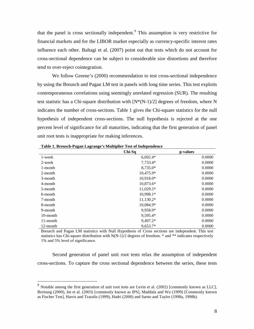
We follow Greene’s (2000) recommendation to test cross-sectional independence

by using the Breusch and Pagan LM test in panels with long time series. This test exploits

contemporaneous correlations using seemingly unrelated regression (SUR). The resulting

test statistic has a Chi-square distribution with [N*(N-1)/2] degrees of freedom, where N

indicates the number of cross-sections. Table 1 gives the Chi-square statistics for the null

hypothesis of independent cross-sections. The null hypothesis is rejected at the one

percent level of significance for all maturities, indicating that the first generation of panel

unit root tests is inappropriate for making inferences.

Second generation of panel unit root tests relax the assumption of independent

cross-sections. To capture the cross sectional dependence between the series, these tests

9 Notable among the first generation of unit root tests are Levin et al. (2002) [commonly known as LLC], Breitung (2000), Im et al. (2003) [commonly known as IPS], Maddala and Wu (1999) [Commonly known as Fischer Test], Harris and Tzaralis (1999), Hadri (2000) and Sarno and Taylor (1998a, 1998b).

Table 1. Breusch-Pagan Lagrange’s Multiplier Test of Independence Chi-Sq p-values 1-week 6,692.4* 0.0000 2-week 7,733.4* 0.0000 1-month 8,735.0* 0.0000 2-month 10,475.9* 0.0000 3-month 10,918.0* 0.0000 4-month 10,873.6* 0.0000 5-month 11,029.5* 0.0000 6-month 10,998.1* 0.0000 7-month 11,130.2* 0.0000 8-month 10,084.9* 0.0000 9-month 9,958.0* 0.0000 10-month 9,595.4* 0.0000 11-month 9,497.2* 0.0000 12-month 9,653.7* 0.0000 Breusch and Pagan LM statistics with Null Hypothesis of Cross sections are independent. This test statistics has Chi-square distribution with N(N-1)/2 degrees of freedom. * and ** indicates respectively 1% and 5% level of significance.

9

model the unobserved common factor across units.10 Underlying this technique is the

premise that variability among observed variables can be described by a potentially lower

number of unobserved variables, called ‘factors’. These common factors are assumed to

account for the variation and co-variation across a range of observed phenomena.

However, the second-generation tests require panels with moderate or large

number of cross-sections with long time series. In addition, these tests can only deal with

common factor structures and contemporaneous dependence. Importantly, as we use a

panel with six cross-sections only, also the application of a second-generation test would

be inappropriate.

The CDRBB test11 does not entail modeling the temporal and/or cross sectional

dependence structures as it uses block bootstrapping. Moreover, the inferences from this

test are valid under a wide range of possible data generating processes, which makes it an

appropriate tool for dealing with the fixed number of cross-sections and large time series

asymptotics. In a nutshell, the block bootstrap technique is the time series version of a

standard bootstrap where the dependence structure of the time series is preserved by

dividing data into blocks and then re-sampling the blocks. However, the block length

selected can have a large effect on the performance of any designed block bootstrap test.

The CDRBB test uses the wrap speed calibration method for selecting the optimal size of

the block.

The CDRBB test provides ‘pooled ( pτ )’ and ‘group-mean ( gmτ )’ test statistics,

summarized by equations (5) and (6), respectively. N and T are the number of cross

sections and time observations, respectively, and ity can refer to exchange rate and

interest rate differential series. The ‘pooled’ statistics presume that the members of the

panel have the same autoregressive coefficient, which is quite restrictive. In other words,

the statistics are obtained by pooling information without considering the individual

member’s characteristics. The ‘group mean’ test statistics, on the other hand, incorporates

the members’ specific individual autoregressive coefficients. Both statistics take as the

null hypothesis that the series is non-stationary vis-à-vis the alternative hypothesis that

10 Widely used second-generation unit root test includes, Bai and Ng (2004), Moon and Perron (2004), Pesaran (2007), and Choi (2005). 11 Proposed by Palm, Smeekes, and Urbain (2010).

10

the series is stationary. Rejection of the null hypothesis when the series are in first

differences and non-rejection of the null when the series are in levels indicates that the

series concerned has a unit root.

(5)

∑

∑∑

=−

=−

=

∆= T

tti

T

ttitiN

igm

y

yyT

N2

21,

2,1,

1

1τ (6)

4.2.2 Panel Cointegration

Cointegration is essentially a method to detect the long-run relationship between

integrated series. UIP requires a positive long-run relationship between interest and

exchange rate differentials. Until recently, the literature has largely adopted residual

based panel cointegration tests, like those proposed by Pedroni (1999; 2004), McCoskey

and Kao (1998; 1999). However, we adopt the Westerlund (2007) error correction based

procedure for testing cointegration for two reasons. First, it presupposes that regressors

are weakly exogenous. In line with this presumption, the UIP hypothesis assumes that the

causality runs contemporaneously from the interest rate to the exchange rate only.

Second, this procedure provides robust critical values for the test statistics by applying

bootstrapping which accounts for the cross sectional dependence.

it

p

jjtiij

p

jjtiijtiitiitiit uxyxydy

ii

+∆+∆+−+=∆ ∑∑=

−=

−−−0

,21

,11,'

1, )( γγβαδ (7)

Westerlund (2007) suggests a panel cointegration test based on the error correction

mechanism (ECM). As shown in Equation (7), id is the currency specific deterministic

component, iδ is the associated parameter, iα is the speed of adjustment for the error

correction term, iβ is the cointegrating vector while itx and ity are interest and exchange

∑∑

∑∑

= =−

=−

=

∆= N

i

T

tti

T

ttiti

N

ip

y

yyT

1 2

21,

2,1,

1τ

11

rate differentials, respectively. It is important to note that the cointegrating vector iβ is

not separately identified here. The choice of the appropriate number of leads and lags,

given by ip , could transform itu into white noise.

The null hypothesis of the cointegration test is 0=iα , which indicates no

cointegration of the variables. Any value of iα less than zero, leads to the rejection of the

null. The statistics αP and τP test the alternative hypothesis that the panel is cointegrated

as a whole.12 Asymptotically, these statistics have a limiting normal distribution and they

are consistent. However, Westerlund (2007) points out that tests for αP have higher

power than those for τP in samples where T is substantially larger than N.

4.2.3 Estimates for Long-run Relationship

To specify the long-run relationship between cointegrated series, various estimation

techniques have been proposed discarding ordinary least squares (OLS). Chen et al.

(1999) have investigated the finite sample properties of OLS as well as the bias corrected

OLS estimators and its t-statistics. They find that the bias corrected OLS estimator does

not improve over the OLS estimator in general and alternatives, such as the Fully

Modified OLS (FMOLS) estimator or the Dynamic OLS (DOLS) estimator, should

therefore be considered for cointegrated panel regressions. Following the suggestion of

Kao and Chiang (2001), we use both panel FMOLS and DOLS. OLS and the bias

corrected OLS results are provided in Appendix 2 for comparison purposes.

The FM-OLS and DOLS estimators provide two forms of estimates. First, by

restricting the slope parameter across individual members to be common ( ββ =i ), the

estimates obtained are called homogenous panel estimates. Second, by allowing the slope

parameters to differ across individual members the estimates obtained are called

12 To capture the individual specific heterogeneity, another set of statistics αG and τG , test the alternative hypothesis that at least one member of the panel is cointegrated. It is also known as Group mean statistics. While the panel statistics are constructed by pooling information the group mean statistics are constructed using individual estimates of coefficients iα ’s and its test statistics (

itα ’s) such as ∑−=

iiNG αα

1 and

∑−=i

iitNG

,

1ατα .

12

heterogeneous panel estimates. We only report the estimates of the homogenous panel as

they are less affected by the small N bias.13

The FM-OLS estimator is constructed by correcting the OLS estimator for

endogeneity and serial correlation. To remove the nuisance parameters, it employs a

semi-parametric correction which results in asymptotically unbiased estimators with fully

efficient mixture normal asymptotics such that the inferences from its limiting

distribution can be drawn easily. The key to the FM-OLS estimation is the construction

of long-run covariance matrix estimators which uses kernel estimates. Originally

proposed by Phillips and Hansen (1990) for time series, the FM-OLS estimator has been

modified for a panel context by Pedroni (2001), Philips and Moon (1999), and Kao and

Chiang (2001).

ititiiit uxy ++= βα (8)

ittiit xx ε+= −1,

For a specification such as equations (8), where all regressors have a unit root and itε is

white noise, the FM-OLS estimator can be given by:

∆−−

−−= ∑∑∑∑

= =

++−

= =

N

i

T

tuititit

N

i

T

tititititFM Tyxxxxxx

1 1

1

1 1)ˆˆ)())((ˆ

εβ (9)

where +∆ uεˆ is a serial correlation correction factor estimated using kernel estimate.

itit

q

qjijitiiit vxxy +∆++= ∑

−=

ςβα ' (10)

The dynamic OLS method removes the nuisance parameters by augmenting the

lags and leads of the regressors. Using equation (10), the DOLSβ̂ can be estimated directly;

it is identically distributed and converges to the same limiting distribution as that of FM-

OLS estimators. McCoskey and Kao (1998) formulate the single equation panel DOLS

using the initial dynamic OLS method proposed by Saikkonen (1992) and Stock and

13 The FM-OLS and DOLS estimators both assume that errors are independent across cross-sections which may not true in this case. In addition, the limiting distribution of both estimators follows the sequential limit theory where ∞→T followed by ∞→N . This assumption is violated in our case, as the number of cross sections (N) is finite. However, estimation techniques for panel-cointegrated systems are still in an evolutionary phase and widely accepted answers to these problems have not yet been provided. Therefore, we apply the DOLS and FMOLS estimators suggested by Kao and Chiang (2001).

13

Watson (1993) for time series. The proposed estimators provide asymptotically efficient

estimates of the cointegrating system. The notations have a similar meaning as in FM-

OLS except for q which represents the number of leads and lags to be incorporated in

(10).

5. Results and Analysis

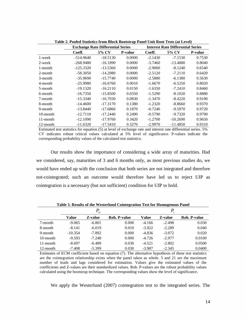
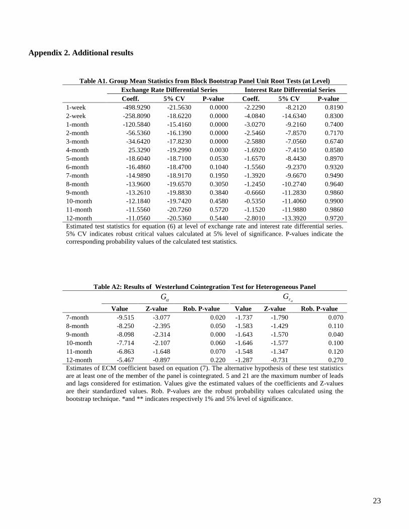
For brevity’s sake, Table 2 reports pooled statistics of the CDRBB test for the level of the

series. The conclusions for group mean statistics are not very different from those based

on pooled statistics and are therefore reported in Appendix 2 (see Table A1). Table 2

shows that the null hypothesis of non-stationary cannot be rejected for the exchange rate

differential series for maturities from 7 to 12-months. The tests for the first difference of

these maturities reject the null hypothesis (not reported), indicating that these series are

I(1). Similarly, for the interest rate differentials, the tests do not (do) reject the null

hypothesis for all (the first difference of) the interest differentials, indicating the series

are I(1). Both exchange and interest rate differentials with maturities between 7 and 12

months are found integrated and therefore subjected to the cointegration test. The other

series are ignored, as panel cointegration tests are useful only for integrated series.

14

Our results show the importance of considering a wide array of maturities. Had

we considered, say, maturities of 3 and 6 months only, as most previous studies do, we

would have ended up with the conclusion that both series are not integrated and therefore

not-cointegrated; such an outcome would therefore have led us to reject UIP as

cointegration is a necessary (but not sufficient) condition for UIP to hold.

We apply the Westerlund (2007) cointegration test to the integrated series. The

Table 2. Pooled Statistics from Block Bootstrap Panel Unit Root Tests (at Level) Exchange Rate Differential Series Interest Rate Differential Series

Coeff. 5% CV P-value Coeff. 5% CV P-value 1-week -514.9640 -18.5130 0.0000 -2.1430 -7.1530 0.7530 2-week -268.9480 -16.1890 0.0000 -3.7460 -13.4880 0.8040 1-month -125.3320 -13.5360 0.0000 -2.9060 -8.1240 0.6540 2-month -58.3050 -14.2080 0.0000 -2.5120 -7.2110 0.6420 3-month -35.9690 -15.7740 0.0000 -2.5880 -6.1380 0.5630 4-month -25.9980 -16.6760 0.0010 -1.6670 -6.5250 0.8020 5-month -19.1320 -16.2110 0.0150 -1.6350 -7.2410 0.8460 6-month -16.7350 -15.8500 0.0350 -1.5290 -8.1020 0.8880 7-month -15.3340 -16.7030 0.0830 -1.3470 -8.4220 0.9190 8-month -14.4600 -17.3170 0.1380 -1.2320 -8.8660 0.9370 9-month -13.8440 -17.6860 0.1870 -0.7240 -9.5970 0.9720 10-month -12.7110 -17.2440 0.2490 -0.5790 -9.7320 0.9790 11-month -12.1090 -17.9760 0.3420 -1.2700 -10.2690 0.9650 12-month -11.6320 -17.5410 0.3270 -2.9970 -11.4850 0.9310 Estimated test statistics for equation (5) at level of exchange rate and interest rate differential series. 5% CV indicates robust critical values calculated at 5% level of significance. P-values indicate the corresponding probability values of the calculated test statistics.

Table 3. Results of the Westerlund Cointegration Test for Homogenous Panel

αP τP

Value Z-value Rob. P-value Value Z-value Rob. P-value 7-month -9.065 -6.801 0.000 -4.166 -2.498 0.030 8-month -8.141 -6.019 0.010 -3.922 -2.289 0.040 9-month -10.354 -7.892 0.000 -4.836 -3.072 0.020 10-month -9.593 -7.248 0.000 -4.726 -2.977 0.0100 11-month -8.697 -6.489 0.030 -4.521 -2.802 0.0500 12-month -7.408 -5.399 0.030 -3.987 -2.345 0.0400 Estimates of ECM coefficient based on equation (7). The alternative hypothesis of these test statistics are the cointegration relationship exists when the panel taken as whole. 5 and 21 are the maximum number of leads and lags considered for estimation. Values give the estimated values of the coefficients and Z-values are their standardized values. Rob. P-values are the robust probability values calculated using the bootstrap technique. The corresponding values show the level of significance.

15

002

003

003

004

004

005

7-m

onth

8-m

onth

9-m

onth

10-m

onth

11-m

onth

12-m

onth

No.

of H

ours

Figure 1: Tenurewise Speed of Adjustment Gα Pα

optimal number of leads and lags to be included in the error correction equation has been

selected based on Akaike’s Information Criterion (AIC). Moreover, critical values are

calculated using bootstrapping. Table 3 shows the panel statistics only. The group-mean

statistics are reported in Table A2 in Appendix 2. Robust p-values for both panel

statistics αP and τP show that the null hypothesis of no cointegration is significantly

rejected at the five percent level of significance. So these tests confirm that there exists a

long-run equilibrium relationship between exchange and interest rate differentials. In

other words, any shock to a currency specific LIBOR rates vis-à-vis another currency

specific rate effects the exchange rates between these currencies in the long run.

It is important to examine the speed of adjustment of the cointegrated series.

Figure 1 shows the adjustment process of the exchange rate for different maturities.14 The

period of adjustment in the exchange rate is found to be increasing in the maturity of the

underlying instruments. For the 7-month maturity the adjustment period is around 159

minutes while for the 12-month maturity it is 194 minutes. The group-mean statistics lead

to similar conclusions. The relatively slow adjustment in 12-month compared to the 7-

month maturity points towards possible arbitrage opportunities, albeit for a very short

period. This finding seems in contrast with the efficient market hypothesis and does not

support the finding of Bekaert et al. (2007). Using both short and long-term debt

instruments, these authors reach the conclusion that the adjustment periods are related to

14 For αG slope coefficient see Table A2 in Appendix 2.

16

currencies and not to the maturities of the underlying instruments.

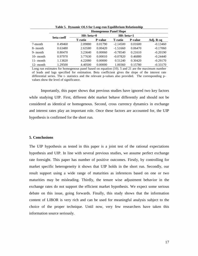
For the cointegrated system Tables 4 and 5 show estimates of the long-run

relationship, using panel FM-OLS and DOLS estimators, respectively. In the FM-OLS

estimates, the non-parametric technique (Bartlett Kernel) is used to estimate the long-run

serial correlation factor. In the DOLS estimates, maximum leads of 5 days and maximum

lags of 21 days have been used, similar to the cointegration test. The FM-OLS and DOLS

estimates show that interest rates differentials are positively related with exchange rate

differentials for all maturities considered (7 to 12 months). This finding is in contrast

with the results of most previous studies which generally report negative beta coefficients

for the short-run horizon.15 In addition, the null hypothesis that beta equals one cannot be

rejected for all maturities, except for a maturity of 7 months. This finding suggests that

UIP holds for the short-run horizon if market specific heterogeneity is controlled for.

Although they are very different, the FM-OLS and DOLS methods provide almost

the same estimate for the slope coefficients and their level of significance. Monte Carlo

simulation results of Kao and Chiang (2001) show that FM-OLS estimates are more

biased compared to DOLS in sample with small N. Furthermore, the negative adjusted R-

square is in line with the existing literature on UIP which generally reports a low or even

negative R-squared (Chinn, 2007).

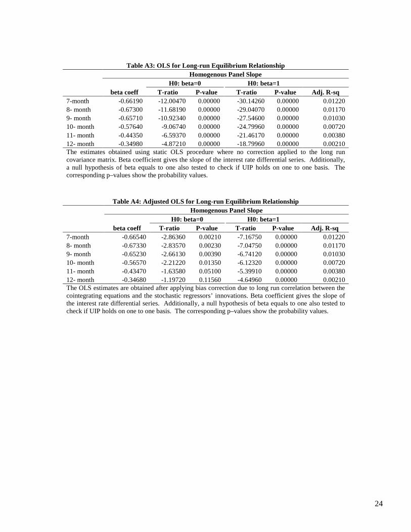
15 Our OLS (see Table A3) and adjusted OLS results (see Table A4) in Appendix 2 also indicate that the slope coefficients are negative and fall in a range generally predicted by empirical research. These results are in line with the findings of earlier studies on UIP.

Table 4. Fully Modified OLS for Long-run Equilibrium Relationship

Homogenous Panel Slope H0: beta=0 H0: beta=1

beta coeff T-ratio P-value T-ratio P-value Adj. R-sq 7-month 0.44560 1.91670 0.02760 -2.38490 0.00850 -0.02220 8- month 0.57160 2.40640 0.00810 -1.80320 0.03570 -0.02850 9- month 0.70690 2.88270 0.00200 -1.19510 0.11600 -0.03450 10- month 0.87680 3.42710 0.00030 -0.48180 0.31500 -0.03900 11- month 1.04500 3.93050 0.00000 0.16920 0.43280 -0.04010 12- month 1.19570 4.12590 0.00000 0.6754 0.2497 -0.04000 Long run estimates for homogenous panel based on equation (8). The estimate of long run variance has used KERNEL in COINT 2.0 with a Bartlett Window. Beta coefficient gives the slope of the interest rate differential series. Additionally, a null hypothesis of beta equals to one also tested to check if UIP holds on one to one basis. The corresponding p–values show the level of significance.

17

Importantly, this paper shows that previous studies have ignored two key factors

while studying UIP. First, different debt market behave differently and should not be

considered as identical or homogenous. Second, cross currency dynamics in exchange

and interest rates play an important role. Once these factors are accounted for, the UIP

hypothesis is confirmed for the short run.

5. Conclusions The UIP hypothesis as tested in this paper is a joint test of the rational expectations

hypothesis and UIP. In line with several previous studies, we assume perfect exchange

rate foresight. This paper has number of positive outcomes. Firstly, by controlling for

market specific heterogeneity it shows that UIP holds in the short run. Secondly, our

result support using a wide range of maturities as inferences based on one or two

maturities may be misleading. Thirdly, the tenure wise adjustment behavior in the

exchange rates do not support the efficient market hypothesis. We expect some serious

debate on this issue, going forwards. Finally, this study shows that the information

content of LIBOR is very rich and can be used for meaningful analysis subject to the

choice of the proper technique. Until now, very few researchers have taken this

information source seriously.

Table 5. Dynamic OLS for Long-run Equilibrium Relationship

Homogenous Panel Slope

beta coeff H0: beta=0 H0: beta=1 T-ratio P-value T-ratio P-value Adj. R-sq

7-month 0.49460 2.09880 0.01790 -2.14500 0.01600 -0.13460 8- month 0.63480 2.63580 0.00420 -1.51660 0.06470 -0.17060 9- month 0.80470 3.23640 0.00060 -0.78540 0.21610 -0.20190 10- month 0.97970 3.77630 0.00010 -0.07820 0.46880 -0.24440 11- month 1.13820 4.22080 0.00000 0.51240 0.30420 -0.29170 12- month 1.29500 4.40500 0.00000 1.00360 0.15780 -0.33170 Long run estimates for homogenous panel based on equation (10). 5 and 21 are the maximum number of leads and lags specified for estimation. Beta coefficient gives the slope of the interest rate differential series. The t- statistics and the relevant p-values also provided. The corresponding p–values show the level of significance.

18

References

Alper, C.E., O.P. Ardic and S. Fendoglu (2009). “The Economics of the Uncovered Interest Rate Parity Condition for Emerging Markets”, Journal of Economic Surveys, 23 (1), 115–138.

Bai, J., and S. Ng (2004). “A PANIC Attack on Unit Roots and Cointegration”, Econometrica, 72 (4), 191-221.

Baillie, R.T. and R. Kilic (2006). “Do Asymmetric and Non-Linear Adjustments Explain the Forward Premium Anomaly?” Journal Of International Money And Finance, 25 (1), 22-47.

Baldwin, R., (1990). “Re-Interpreting the Failure of Foreign Exchange Market Efficiency Tests: Small Transaction Costs, Big Hysteresis Bands”, NBER Working Paper 3319.

Baltagi, B. H., G. Bresson and A. Pirotte, (2007). “Panel Unit Root Tests and Spatial Dependence”, Journal of Applied Econometrics, 22 (2), 339-360.

Bansal, R. and M. Dahlquist (2000). “The Forward Premium Puzzle, Different Tales from Developed and Emerging Economies”, Journal of International Economics, 51, 115-144.

Bekaert, G., M. Wei and Y. Xing (2007). “Uncovered Interest Rate Parity and the Term Structure”, Journal of International Money and Finance, 26 (6), 1038-1069.

Brace, A., D. Gatarek, , and M. Musiela (1997). “The Market Model of Interest Rate Dynamics”, Mathematical Finance, 7, 127–155.

Branson, W. H. and D. W. Henderson (1985). “The Specification And Influence Of Assets Markets.” In: Kenen, P.B. and R.W. Jones, (Eds.), Handbook Of International Economics, Amsterdam: North Holland, pp. 749-805

Breitung, J. (2000). “The Local Power of Some Unit Root Tests for Panel Data.” In B. H. Baltagi (Ed.), On the Estimation and Inference of a Cointegrated Regression in Panel Data. 222 Amsterdam: Elsevier, Vol. Advances in Econometrics 15, pp. 161–177.

Bruggemann, R. and H. Lutkepohl (2005). “Uncovered Interest Rate Parity and the Expectation Hypothesis of the Term Structure: Empirical Results for the US and Europe.” Applied Economics Quarterly, 51(2), 143-154.

Campbell, R., K. Koedijk, J. R. Lothian and R. J. Mahieu (2007). “Irving Fisher, Expectational Error, and the UIP Puzzle”, CEPR Discussion Paper 6294.

Candelon, B. and L. Gil –Alana (2006). “Mean Reversion of Short-run Interest Rates in Emerging Countries”, Review of International Economics, 14(1), 119–135.

Carlson, J.A. and C.L. Osler (1999). “Determinants Of Currency Premiums.” Mimeo, Federal Reserve Bank Of New York (February).

Carvalho, J.C., A. Sachsida, P. R. A. Loureiro and T. B. S. Moreira (2004). “Uncovered Interest Rate Parity in Argentina, Brazil, Chile and Mexico: A Unit Root Test Application with Panel Data”, Review of Urban & Regional Development Studies, 16 (3), 263-269.

Chaboud, A. P., and J. H. Wright (2005). “Uncovered Interest Parity, It Works, But Not For Long”, Journal of International Economics, 66(2), 349-362.

Chen, W. B., S. K. McCoskey and C. Kao (1999). “Estimation and Inference of a Cointegrated Regression in Panel Data: A Monte Carlo Study,” American Journal of Mathematical and Management Sciences, 19(1), 75-114.

19

Chinn, M. D., and G. Meredith (2004). “Monetary Policy and Long Horizon Uncovered Interest Parity”, IMF Staff Papers, 51(3), 409-430.

Chinn, M. D., and G. Meredith (2005). “Testing Uncovered Interest Parity at Short And Long Horizons During The Post-Bretton Woods Era”, NBER Working Paper 11077.

Chinn, M.D. (2007). ” Interest Rate Parity 4”, Entry Written for Princeton Encyclopedia of the World Economy.

Choi, I., (2005). “Combination of Unit Root Tests for Cross-sectionally Correlated Panels”. In: D. Corbae, S. N. Durlauf and B. E. Hansen (Eds.), Econometric Theory and Practice: Frontiers of Analysis and Applied Research, Cambridge: Cambridge University Press, pp. 311-333.

De Haan, J., D. Pilat and D. Zelhorst (1992). “On the Relationship Between Dutch and German Interest Rates”, De Economist, 139(4), 550-565.

De Long, J.B., A. Shleifer, L.H. Summers and R.J. Waldmann (1990). “Noise Trader Risk In Financial Markets”, Journal of Political Economy, 98, 703-738.

Dreger, C., (2010). “Does The Nominal Exchange Rate Regime Affect the Real Interest Parity Condition?” North American Journal of Economics and Finance, doi:10.1016/j.najef.2010.01.001

Dumas, B., (1992). “Dynamic Equilibrium And The Real Exchange Rate In A Spatially Separated World”, Review Of Financial Studies, 5, 153-80.

Engel, C., (1996). “The Forward Discount Anomaly and the Risk Premium: A Survey of Recent Evidence”, Journal of Empirical Finance, 3, 123-92.

Flood, R. P., and A. K Rose (1996). “Fixes, of the Forward Discount Puzzle”, Review of Economics and Statistics, 78(4), 748-752.

Flood, R. P., and M. P. Taylor (1996). “Exchange Rate Economics: What’s Wrong With the Conventional Macro Approach?” In: J. Frankel, G. Galli and A. Giovannini (Eds.), The Microstructure Of Foreign Exchange Markets, Chicago: University of Chicago Press, pp. 262-301.

Frankel, J. A., (1983). “Monetary And Portfolio Balance Models Of Exchange Rate Determination.” In: Bhandari, J.S. and B.H. Putnam (Eds.), Economic Interdependence And Flexible Exchange Rates, Chicago: MIT Press, pp. 84-115.

Frankel, J. A., (1984). “The Yen/Dollar Agreement: Liberalizing Japanese Capital Markets”, Policy Analyses in International Economics 9, Washington, D.C.; Institute for International Economics.

Frankel, J. A., and K. A. Froot (1989). “Forward Discount Bias: Is it an Exchange Risk Premium?”, The Quarterly Journal Of Economics, 104, 139-161.

Froot, K. A., and R. H. Thaler (1990). “Anomalies: Foreign Exchange”, Journal of Economic Perspectives, 4, 179–192.

Greene, W., (2000). Econometric Analysis. Upper Saddle River, NJ: Prentice-Hall. Hadri, K., (2000). “Testing for Stationarity in Heterogeneous Panel Data”, Econometrics

Journal, 3, 148–161. Harmantzis, F.C and J. S. Nakahara (2007). “Evidence of Persistence in the London

Interbank Offer Rate”, FMA European Conference Program, May 30 to June 01. Harri, A. and W. Brorsen (2002). “The overlapping data problem”, Quantitative and

Qualitative Analysis in Social Sciences, 3(3), 78-115.

20

Harris, R. D. F., and E. Tzavalis (1999). “Inference for Unit Roots in Dynamic Panels where the Time Dimension is Fixed”, Journal of Econometrics, 91, 201-226.

Harvey, J. T., (2005). “Deviations from Uncovered Interest Rate Parity: A Post Keynesian Explanation”, Journal of Post Keynesian Economics, 27(1), 19-35.

Ichiue, H., and K. Koyama (2007). “Regime Switches in Exchange Rate Volatility and Uncovered Interest Parity”, Bank of Japan Working Paper No. 07-E-22.

Im, K. S., M. H. Pesaran and Y. Shin (2003). “Testing for Unit Roots in Heterogeneous Panels”, Journal of Econometrics, 115 (1), 53-74.

Isard, P., (1996). “Uncovered Interest Parity”, IMF Working Paper 06/96. Jamshidian, F., (1997). “LIBOR and Swap Market Models and Measures”, Finance and

Stochastics, 1, 293-330. Juselius, K. and R. MacDonald (2004). “International Rarity Relationship Between the

USA and Japan”, Japan and the World Economy, 16, 17–34. Kao, C., (1999). “ Spurious Regression and Residual-Based Tests for Cointegration in

Panel data”, Journal of Econometrics, 90, 1-44. Kao, C., and M. Chiang (2001). “Nonstationary Panels, Cointegration in Panels and

Dynamic Panels.” In B. H. Baltagi (Ed.), On the Estimation and Inference of a Cointegrated Regression in Panel Data. 222 Amsterdam: Elsevier, Vol. Advances in Econometrics, 15, pp. 179 -222.

Krishnakumar, J., and D. Neto (2008). “Testing Uncovered Interest Rate Parity and Term Structure Using Multivariate Threshold”, Computational Methods in Financial Engineering, Part II: 191-210.

Kwan, S., (2009). “Behavior of Libor in the Current Financial Crisis”, FRBSF Economic Letters, Nov 04th – Jan 23rd. Levin, A., C. Lin and C. J. Chu (2002). “Unit Root Tests in Panel Data: Asymptotic and

Finite-Sample Properties”, Journal of Econometrics, 108, 1-24. Lewis, K. K., (1989). “Changing Beliefs and Systematic Rational Forecast Errors With

Evidence From Foreign Exchange”, American Economic Review, 79, 621-636. Lewis, K. K., (1995). “Puzzles In International Financial Markets.” In: Grossman, G.M.

and K. Rogoff (Eds.), Handbook Of International Economics Vol. 3. Amsterdam: Elsevier, pp. 1913– 1949.

MacDonald, R., and M. P. Taylor (1992). “Exchange Rate Economics: A Survey”, IMF Staff Papers, 39 (1), 1-57.

Maddala, G. S., and S. Wu (1999). ”A Comparative Study of Unit Root Tests With Panel Data and a New Simple Test”, Oxford Bulletin of Economics and Statistics, 61 (Special Issue), 631-652.

Mariscal, I. B., and P. Howells (2002). “Central Banks and Market Interest Rates”, Journal of Post Keynesian Economics, 24(4), 569-585.

Mark, N., and Y. Wu (1998). “Rethinking Deviations From Uncovered Interest Parity: The Role of Covariance Risk And Noise.” The Economic Journal, 108 (451), 1686-1706.

McCallum, B.T., (1994). “A Reconsideration of The Uncovered Interest Parity Relationship”, Journal Of Monetary Economics, 33, 105-32.

McCoskey, S., and C. Kao (1998). “A Residual-based Test of the Null of Cointegration in Panel Data”, Econometric Reviews, 17(1), 57- 84

21

Michaud, F. L., and C. Upper (2008). “ What Drives Interbank Rates? Evidence from Libor Panel”, BIS Quarterly Review, March 2008, 47-58.

Miltersen, K. R., K. Sandmann, and D. Sondermann (1997). “Closed Form Solutions for Term Structure Derivatives With Log-normal Interest Rates”, The Journal of Finance, 52, 409–430.

Moon, H., and B. Perron (2004). “Testing for a Unit Root in Panels with Dynamic Factors”, Journal of Econometrics, 122, 81-126.

Palm, F. C., S. Smeekes, and J-P. Urbain (2010). “Cross-sectional Dependence Robust Block Bootstrap Panel Unit Root Tests”, Journal of Econometrics. doi:10.1016/j.jeconom.2010.11.010

Pasricha, G. M., (2006). “Survey of literature on Covered and Uncovered Interest Rate Parities”, MPRA Paper 22737.

Pedroni, P., (1999). “Critical Values for Cointegration Tests in Heterogeneous Panels With Multiple Regressors”, Oxford Bulletin of Economics and Statistics, 61, 653-670.

Pedroni, P., (2001). “Fully Modified OLS for Heterogeneous Cointegrated Panels”, in Badi H. Baltagi, Thomas B. Fomby, R. Carter Hill (ed.) Nonstationary Panels, Panel Cointegration, and Dynamic Panels (Advances in Econometrics, Volume 15), Emerald Group Publishing Limited, pp. 93-130

Pedroni, P., (2004). “Panel Cointegration: Asymptotic and Finite Sample Properties of Pooled Time-series Tests with Application to the PPP Hypothesis”, Econometric Theory, 20, 597–625

Pesaran, M. H., (2007). “A Simple Panel Unit Root Test in the Presence of Cross-Section Dependence”, Journal of Applied Econometrics, 22 (2), 265-312.

Phillips, P. C. B., and B. E. Hansen (1990). “Statistical Inference in Instrumental Variables Regression with I(1) Processes”, Review of Economic Studies, 57 (1), 99-125.

Phillips, P. C. B., and H. R. Moon (1999). “Linear Regression Limit Theory for Non -stationary Panel Data”, Econometrica, 67 (5), 1057-1112.

Saikkonen, P., (1992). “Estimation and Testing of Cointegrated System by an Autoregressive Approximation,” Econometric Theory, 8, 1-27.

Sarno, L., and M. Taylor (1998a). “Real Exchange Rates Under the Current Float: Unequivocal Evidence of Mean Reversion”, Economics Letters, 60, 131–137.

Sarno, L., and M. Taylor (1998b). “The Behavior of Real Exchange Rates During the Post Bretton Woods Period”, Journal of International Economics, 46, 281–312.

Sarno, L., G. Valente and H. Leon (2006). “The Forward Bias Puzzle And Nonlinearity in Deviations From Uncovered Interest Parity: A New Perspective”, CEPR Discussion Paper 5527.

Stock, J. H., and M. W. Watson (1993). “A simple Estimator of Cointegration Vectors in Higher Order Integrated Systems”, Econometrica, 61, 783-820.

Tang, K.-B., (2010). “The Precise Form of Uncovered Interest Parity: A Heterogeneous Panel Application in ASEAN-5 Countries”, Economic Modelling, doi:10.1016/j.econmod.2010.06.015

Westerlund, J., (2007).“Testing for Error Correction in Panel Data”, Oxford Bulletin of Economic and Statistics, 69 (6), 709-48.

22

Appendix 1. Literature Review

Author (s) Period Est. Type Currency/Country

Horizon Interest Rate Variable Methodology Conclusion De Haan, Pilat and Zelhorst .(1992)

1979 M10-1989 M6; Monthly Time series

Dutch/German Exchange Rate

3-months Euro deposit rates and Amsterdam interbank rate

Unit Roots and Cointegration Rejected

Baillie and Kilic (2006) 1978- 1998/2002; Monthly

Ind. Time Series 9 currencies BIS; end month asked rates

Dynamic smooth transition regression Mixed

Bansal and Dahlquist (2000).

1976 M1 to 1998 M5 Pooled

28 (Emerging and Developed

Spot Exchange Rate, Forward Rate, Interest Rate Pooled OLS Mixed

Bekaert, Wei and Xing (2007)

1972-1991; Monthly

Ind. Time Series

3 currencies, US, UK and Germany

Jorion and Mishkin (1991) dataset VAR Analysis Mixed

Bruggemann and Lutkepohl (2005)

1985 M1-2004 M12; Monthly

Ind. Time Series Euro Vs USD

3-m Money Market Rates and 10-years Bonds VECM

Supports UIP

Carvalho, Sachsida, Loureiro and Moreira (2004)

1990-2001; Monthly Panel

4 currencies (Argentina, Brazil, Chile and Mexico)

Domestic Interest rates and official exchange rates

fixed and random effects Mixed

Chaboud and Wright (2005)

1988-2002; high freq. data (5-min interval) Time Series

JPY, Euro(DM), CHF, GBP against USD

Reuter Quotes at 5 min for ER and Overnight rate OLS Mixed*

Chinn and Meredith (2004) 1980-2000; Quarterly Panel G-7 countries

3-, 6- and 12- m exchange rate movement; GMM Mixed**

Flood and Rose (1996) 1981- 1994; daily Pooled

Australia; Canada; France; Germany; Japan; Switzerland; & UK all against US

1- and 3- months Interest rate differential ; 1- and 3-months exchange rate movements SUR technique UIP holds

Campbell, Koedijk, Lothian and Mahieu (2007)

1970 M1- 2005 M12; Monthly

Individual Time Series

18 currencies against USD

Short term domestic treasury bills or money market rates

Standard and Rolling regression Rejected

Candelon and Gil -Alana (2006)

1980 M1 - 2001 M12; Monthly

Ind. Time Series 6 Emerging economies Short-term interest rates

Fractional Integration Technique Mixed

Harvey (2005) 1989-1998; Quarterly

Ind. Time Series USD- DM and USD- JPY

I-month LIBOR on USD, DM and JPY Simple regression Rejected

Ichiue and Koyama (2007) 1980-2007; Monthly Pooled

JPY, GBP, CHF and DM against USD IFS and LIBOR Regime Switching Mixed

Tang (2010) 1978Q1-2008Q4 Panel Asean-5 IFS Panel Unit root and cointegration Mixed

Juselius and MacDonald (2004) 1975 M7- 1998 M1 Time series USD-JPY Long Bond rates and LIBOR VAR Analysis Rejected

Mark and Wu (1998) 1976 M1 to 1994 M1; Quarterly

Ind. Time Series USD, GBP, DM, JPY - VECM Rejected

Krishnakumar and Neto (2008)

1986 M1 - 2007 M2; Monthly Time series USD - CHF

3-month for short term and 1-year for long term interest rates Threshold vector ECM

Supports UIP

* UIP accepted over very short windows of data that span the time of the discrete interest payment. However, adding even a few hours to the span window destroyed the positive UIP results.; ** Reject in the short run, more support in the long run

23

Appendix 2. Additional results

Table A1. Group Mean Statistics from Block Bootstrap Panel Unit Root Tests (at Level) Exchange Rate Differential Series Interest Rate Differential Series Coeff. 5% CV P-value Coeff. 5% CV P-value 1-week -498.9290 -21.5630 0.0000 -2.2290 -8.2120 0.8190 2-week -258.8090 -18.6220 0.0000 -4.0840 -14.6340 0.8300 1-month -120.5840 -15.4160 0.0000 -3.0270 -9.2160 0.7400 2-month -56.5360 -16.1390 0.0000 -2.5460 -7.8570 0.7170 3-month -34.6420 -17.8230 0.0000 -2.5880 -7.0560 0.6740 4-month 25.3290 -19.2990 0.0030 -1.6920 -7.4150 0.8580 5-month -18.6040 -18.7100 0.0530 -1.6570 -8.4430 0.8970 6-month -16.4860 -18.4700 0.1040 -1.5560 -9.2370 0.9320 7-month -14.9890 -18.9170 0.1950 -1.3920 -9.6670 0.9490 8-month -13.9600 -19.6570 0.3050 -1.2450 -10.2740 0.9640 9-month -13.2610 -19.8830 0.3840 -0.6660 -11.2830 0.9860 10-month -12.1840 -19.7420 0.4580 -0.5350 -11.4060 0.9900 11-month -11.5560 -20.7260 0.5720 -1.1520 -11.9880 0.9860 12-month -11.0560 -20.5360 0.5440 -2.8010 -13.3920 0.9720 Estimated test statistics for equation (6) at level of exchange rate and interest rate differential series. 5% CV indicates robust critical values calculated at 5% level of significance. P-values indicate the corresponding probability values of the calculated test statistics.

Table A2: Results of Westerlund Cointegration Test for Heterogeneous Panel

αG ατG

Value Z-value Rob. P-value Value Z-value Rob. P-value 7-month -9.515 -3.077 0.020 -1.737 -1.790 0.070 8-month -8.250 -2.395 0.050 -1.583 -1.429 0.110 9-month -8.098 -2.314 0.000 -1.643 -1.570 0.040 10-month -7.714 -2.107 0.060 -1.646 -1.577 0.100 11-month -6.863 -1.648 0.070 -1.548 -1.347 0.120 12-month -5.467 -0.897 0.220 -1.287 -0.731 0.270 Estimates of ECM coefficient based on equation (7). The alternative hypothesis of these test statistics are at least one of the member of the panel is cointegrated. 5 and 21 are the maximum number of leads and lags considered for estimation. Values give the estimated values of the coefficients and Z-values are their standardized values. Rob. P-values are the robust probability values calculated using the bootstrap technique. *and ** indicates respectively 1% and 5% level of significance.

24

Table A3: OLS for Long-run Equilibrium Relationship

Homogenous Panel Slope H0: beta=0 H0: beta=1

beta coeff T-ratio P-value T-ratio P-value Adj. R-sq 7-month -0.66190 -12.00470 0.00000 -30.14260 0.00000 0.01220 8- month -0.67300 -11.68190 0.00000 -29.04070 0.00000 0.01170 9- month -0.65710 -10.92340 0.00000 -27.54600 0.00000 0.01030 10- month -0.57640 -9.06740 0.00000 -24.79960 0.00000 0.00720 11- month -0.44350 -6.59370 0.00000 -21.46170 0.00000 0.00380 12- month -0.34980 -4.87210 0.00000 -18.79960 0.00000 0.00210 The estimates obtained using static OLS procedure where no correction applied to the long run covariance matrix. Beta coefficient gives the slope of the interest rate differential series. Additionally, a null hypothesis of beta equals to one also tested to check if UIP holds on one to one basis. The corresponding p–values show the probability values.

Table A4: Adjusted OLS for Long-run Equilibrium Relationship

Homogenous Panel Slope H0: beta=0 H0: beta=1

beta coeff T-ratio P-value T-ratio P-value Adj. R-sq 7-month -0.66540 -2.86360 0.00210 -7.16750 0.00000 0.01220 8- month -0.67330 -2.83570 0.00230 -7.04750 0.00000 0.01170 9- month -0.65230 -2.66130 0.00390 -6.74120 0.00000 0.01030 10- month -0.56570 -2.21220 0.01350 -6.12320 0.00000 0.00720 11- month -0.43470 -1.63580 0.05100 -5.39910 0.00000 0.00380 12- month -0.34680 -1.19720 0.11560 -4.64960 0.00000 0.00210 The OLS estimates are obtained after applying bias correction due to long run correlation between the cointegrating equations and the stochastic regressors’ innovations. Beta coefficient gives the slope of the interest rate differential series. Additionally, a null hypothesis of beta equals to one also tested to check if UIP holds on one to one basis. The corresponding p–values show the probability values.