Purdue UniversityPurdue e-Pubs

Open Access Dissertations Theses and Dissertations

12-2016

Observability and observer design for switchedlinear systemsScott C. JohnsonPurdue University

Follow this and additional works at: https://docs.lib.purdue.edu/open_access_dissertations

Part of the Electrical and Computer Engineering Commons

This document has been made available through Purdue e-Pubs, a service of the Purdue University Libraries. Please contact epubs@purdue.edu foradditional information.

Recommended CitationJohnson, Scott C., "Observability and observer design for switched linear systems" (2016). Open Access Dissertations. 952.https://docs.lib.purdue.edu/open_access_dissertations/952

brought to you by COREView metadata, citation and similar papers at core.ac.uk

provided by Purdue E-Pubs

OBSERVABILITY AND OBSERVER DESIGN

FOR SWITCHED LINEAR SYSTEMS

A Dissertation

Submitted to the Faculty

of

Purdue University

by

Scott C. Johnson

In Partial Fulfillment of the

Requirements for the Degree

of

Doctor of Philosophy

December 2016

Purdue University

West Lafayette, Indiana

ii

This thesis is dedicated to my wife, April. Her patience and steadfast

encouragement has made this journey possible.

iii

ACKNOWLEDGMENTS

The author would like to thank Dr. Raymond DeCarlo for his commitment to

research at the highest level attainable. The author would also like to thank Dr.

Richard T. Meyer, Dr. Steven Pekarek, and Dr. Milos Zefran for helpful advice and

encouragement along the way. The author has been graciously supported financially

by the Graduate School, Electrical and Computer Engineering Department, and the

Department of Energy in collaboration with Dr. Gregory Shaver and the Hoosier

Heavy Hybrid Center of Excellence.

iv

TABLE OF CONTENTS

Page

LIST OF TABLES . . . . . . . . . . . . . . . . . . . . . . . . . . . . . . . . vii

LIST OF FIGURES . . . . . . . . . . . . . . . . . . . . . . . . . . . . . . . viii

ABSTRACT . . . . . . . . . . . . . . . . . . . . . . . . . . . . . . . . . . . x

1 INTRODUCTION AND PROBLEM STATEMENT . . . . . . . . . . . . 1

1.1 Motivation . . . . . . . . . . . . . . . . . . . . . . . . . . . . . . . . 2

1.2 Definitions, Assumptions, and Problem Statement . . . . . . . . . . 3

1.3 Embedded MHO Problem Statement . . . . . . . . . . . . . . . . . 5

2 OBSERVABILITY OF SWITCHED SYSTEMS . . . . . . . . . . . . . . 11

2.1 LTI System Background . . . . . . . . . . . . . . . . . . . . . . . . 11

2.1.1 Review of LTI System Observability Results . . . . . . . . . 11

2.1.2 Disturbance Decoupling Problem For LTI Systems . . . . . . 13

2.2 SMS Observability of SLTI Systems . . . . . . . . . . . . . . . . . . 16

2.2.1 Without Input . . . . . . . . . . . . . . . . . . . . . . . . . 16

2.2.2 With Input . . . . . . . . . . . . . . . . . . . . . . . . . . . 20

2.3 Set-Transition Observability . . . . . . . . . . . . . . . . . . . . . . 25

2.3.1 Examples . . . . . . . . . . . . . . . . . . . . . . . . . . . . 27

2.4 Observability of Switched Linear Time-Varying Systems . . . . . . . 30

2.4.1 Without a Continuous Input . . . . . . . . . . . . . . . . . . 31

2.4.2 Observability with Input . . . . . . . . . . . . . . . . . . . . 36

2.4.3 Extensions to Nonlinear Switched Systems . . . . . . . . . . 41

2.4.4 Conclusions . . . . . . . . . . . . . . . . . . . . . . . . . . . 43

2.5 Appendix for Section 2.3 . . . . . . . . . . . . . . . . . . . . . . . . 43

3 STRUCTURED ROBUST PROPERTY METRIC: P-ROBUSTNESS . . 48

3.1 Introduction . . . . . . . . . . . . . . . . . . . . . . . . . . . . . . . 48

v

Page

3.2 P-Robustness Problem . . . . . . . . . . . . . . . . . . . . . . . . . 51

3.3 Necessary Conditions . . . . . . . . . . . . . . . . . . . . . . . . . . 55

3.4 P-Robustness Algorithm . . . . . . . . . . . . . . . . . . . . . . . . 65

3.4.1 Algorithm 1 Implementation . . . . . . . . . . . . . . . . . . 71

3.5 Convergence of Algorithm 1 . . . . . . . . . . . . . . . . . . . . . . 73

3.6 Numerical Examples . . . . . . . . . . . . . . . . . . . . . . . . . . 78

3.6.1 Example 1 . . . . . . . . . . . . . . . . . . . . . . . . . . . . 78

3.6.2 Example 2 . . . . . . . . . . . . . . . . . . . . . . . . . . . . 79

3.7 Conclusion . . . . . . . . . . . . . . . . . . . . . . . . . . . . . . . . 80

3.8 Chapter 3 Appendix . . . . . . . . . . . . . . . . . . . . . . . . . . 80

3.8.1 Surjectivity . . . . . . . . . . . . . . . . . . . . . . . . . . . 80

3.8.2 Additional Proofs . . . . . . . . . . . . . . . . . . . . . . . . 86

4 SWITCHED SYSTEM OBSERVERS: REVIEW AND PROPOSED SOLU-TION . . . . . . . . . . . . . . . . . . . . . . . . . . . . . . . . . . . . . 94

4.1 Switched System Observer Review . . . . . . . . . . . . . . . . . . . 96

4.1.1 Bank of State Observers . . . . . . . . . . . . . . . . . . . . 96

4.1.2 Moving Horizon Observers . . . . . . . . . . . . . . . . . . . 98

4.2 New Results Moving Horizon Observer . . . . . . . . . . . . . . . . 102

4.2.1 Time-Invariant Switched MHO (SMHO) . . . . . . . . . . . 102

4.2.2 Embedded LTI without Input . . . . . . . . . . . . . . . . . 106

4.2.3 Embedded LTV without Input . . . . . . . . . . . . . . . . . 111

4.2.4 Embedded LTI with Input . . . . . . . . . . . . . . . . . . . 113

4.2.5 Embedded LTV with Input . . . . . . . . . . . . . . . . . . 117

4.2.6 EMHO Convergence . . . . . . . . . . . . . . . . . . . . . . 118

5 FAULT DETECTION IN SPMSM WITH APPLICATIONS TO HEAVYHYBRID VEHICLES . . . . . . . . . . . . . . . . . . . . . . . . . . . . . 121

5.1 Introduction and Motivation . . . . . . . . . . . . . . . . . . . . . . 121

5.1.1 Faults in a Permanent Magnet Synchronous Machine . . . . 121

5.1.2 Chapter Objectives . . . . . . . . . . . . . . . . . . . . . . . 122

vi

Page

5.1.3 Recasting the Observer Problem in a Switched System Observ-ability Setting . . . . . . . . . . . . . . . . . . . . . . . . . . 124

5.1.4 Review of Switched System Observability Results . . . . . . 125

5.1.5 Application to ITSC Fault Observability . . . . . . . . . . . 127

5.2 Surface PMSM without Fault . . . . . . . . . . . . . . . . . . . . . 128

5.2.1 Extensions to Supervisory Powerflow Modeling . . . . . . . . 132

5.3 Extended Matrix Equations: Modeling ITSC Fault in Surface PMSM 133

5.3.1 ITSC Fault Equation Description . . . . . . . . . . . . . . . 133

5.3.2 Extensions to Supervisory Powerflow Modeling: Fault Case . 135

5.3.3 Fault Current Simulation . . . . . . . . . . . . . . . . . . . . 136

5.4 Nominal Fault Detection Observer . . . . . . . . . . . . . . . . . . . 142

5.4.1 ITSC Observer Problem Statement . . . . . . . . . . . . . . 142

5.4.2 Moving Horizon Observer . . . . . . . . . . . . . . . . . . . 144

5.4.3 ITSC Observability . . . . . . . . . . . . . . . . . . . . . . . 146

5.4.4 Nominal ITSC Observer . . . . . . . . . . . . . . . . . . . . 149

5.5 Practical Observer Implementation . . . . . . . . . . . . . . . . . . 154

5.6 Simulation Results . . . . . . . . . . . . . . . . . . . . . . . . . . . 156

5.7 Application: Heavy Hybrid Vehicles . . . . . . . . . . . . . . . . . . 162

5.7.1 Increased Scale . . . . . . . . . . . . . . . . . . . . . . . . . 163

5.7.2 Interior PMSM . . . . . . . . . . . . . . . . . . . . . . . . . 163

5.7.3 Fault-Tolerant Control . . . . . . . . . . . . . . . . . . . . . 166

5.8 Future Work . . . . . . . . . . . . . . . . . . . . . . . . . . . . . . . 166

6 FUTURE WORK . . . . . . . . . . . . . . . . . . . . . . . . . . . . . . . 171

6.1 Robust Observability Extensions . . . . . . . . . . . . . . . . . . . . 171

6.2 EMHO Extensions . . . . . . . . . . . . . . . . . . . . . . . . . . . 173

REFERENCES . . . . . . . . . . . . . . . . . . . . . . . . . . . . . . . . . . 175

VITA . . . . . . . . . . . . . . . . . . . . . . . . . . . . . . . . . . . . . . . 181

vii

LIST OF TABLES

Table Page

5.1 Simulation and SPMSM Parameters . . . . . . . . . . . . . . . . . . . 158

5.2 ITSC EMHO Parameters . . . . . . . . . . . . . . . . . . . . . . . . . . 159

viii

LIST OF FIGURES

Figure Page

1.1 The moving horizon observer scheme with horizon T with uniform time δbetween subsequent horizons. The estimator output y(t) depends on thestate estimate x(t− h) and mode estimate v(t) over the current optimiza-tion horizon. . . . . . . . . . . . . . . . . . . . . . . . . . . . . . . . . . 6

1.2 Bank of observers each producing a state estimate xi with the overall stateand mode estimate based on a decision process using estimator outputs yiand measured outputs y. . . . . . . . . . . . . . . . . . . . . . . . . . . 7

3.1 This figure illustrates the first necessary condition. Given appropriateassumptions, the surface Lu∗V∗(·) = 0 is tangent to the curve σn(M−R∗−δM) = 0 for δM ∈ S at M − R∗ − δM∗, where u∗ is the nth lsv and V∗ isthe nth through mth rsv ofM−R∗−δM∗. For δM∗ to be a local minimumrank reducing perturbation for the property matrix R∗ the line connectingM − R∗ to M − R∗ − δM∗ must be perpendicular to the tangent surfaceLu∗V∗(·) = 0. . . . . . . . . . . . . . . . . . . . . . . . . . . . . . . . . 57

3.2 This figure illustrates the simply-connected neighborhood W of (ζ0, ρ0)partitioned three simply connected regions: W1 and W2 disjoint open setswith W ⊂ cl(W1 ∪W2) and the surface W ∩ {σn(·) = 0}. . . . . . . . . 60

5.1 This figure is a cross-sectional illustration of the SPMSM. The SPMSMhas permanent magnets on the surface of the rotor and coils wound intothe stator. Typically, SPMSM have more than two permanent magnetsfixed to the rotor surface, unlike the two shown for illustrative purposes. 128

5.2 The SPMSM stator connected to the DC-AC inverter. The wye config-uration of the SPMSM stator winding is wound with a neutral point asshown on the right. As illustrated on the far left, the negative rail maynot be connected to ground directly. . . . . . . . . . . . . . . . . . . . 129

5.3 SPMSM rotor connected to mechanical load. The rotor position is denotedθm and load torque TL. . . . . . . . . . . . . . . . . . . . . . . . . . . . 131

5.4 Fault current for various degrees of fault. The fault of severity σf occursat 0.5s. The lower figure zooms in on the interval surrounding 0.5s to seethe difference between each level of fault severity. . . . . . . . . . . . . 137

ix

Figure Page

5.5 Stator voltages for various degrees of fault. The fault of severity σf occursat 0.5s. The stator voltage is assumed to be chosen to maintain statorcurrents given in (5.49). . . . . . . . . . . . . . . . . . . . . . . . . . . 139

5.6 (top) Plot of the inverter supplied power Pinv for various degrees of fault.The fault of severity σf occurs at 0.5s. (bottom) Plot of the electromag-netic power Pabcf for various degrees of fault. The average electromagneticpower is also computed as an average instantaneous power over the window[t− Tperiod, t]. . . . . . . . . . . . . . . . . . . . . . . . . . . . . . . . . 140

5.7 (top) Plot of the average inverter supplied power Pinv for various degreesof fault. The average power is computed as the average instantaneouspower over a window [t − Tperiod, t] for each time t, where Tperiod = 2π

ωris

the period. The fault of severity σf occurs at 0.5s. (bottom) Plot of theaverage electromagnetic power Pabcf for various degrees of fault. The av-erage electromagnetic power is also computed as an average instantaneouspower over the window [t− Tperiod, t]. . . . . . . . . . . . . . . . . . . 141

5.8 The fault detection observer uses known control input u, measured outputyM , and the ITSC fault model to produce an estimate for the degree offault σ and the fault current ifs. . . . . . . . . . . . . . . . . . . . . . . 142

5.9 (A) and (B) illustrate how the previous horizon estimate iabcf (tk − h1) isintegrated forward to hot-start iabcf (tk+1 − h1) when h1 ≥ Tshift. Notice,that the integration is within the interval [tk−T, tk]. (C) and (D) illustratewhen h2 < Tshift. Note, that the integration is not contained in [tk−T, tk].. . . . . . . . . . . . . . . . . . . . . . . . . . . . . . . . . . . . . . . . 153

5.10 This figure shows how the final estimates for partitions in the horizon[tk − T, tk] are used as initial estimates for the horizon [tk+1 − T, tk+1]. . 157

5.11 The fault current reconstruction error |ifs− ifs| is simulated for four levelsof fault, σf = 0.01, 0.02, 0.05, and 0.1. The figure is normalized by max(ifs)which represents the magnitude of the steady state fault current ifs foreach degree of fault. In each simulation, the fault occurs at 0.5s. . . . 160

5.12 The degree of fault reconstruction error |σ− σ| is simulated for four levelsof fault, σf = 0.01, 0.02, 0.05, and 0.1. In each simulation, the fault occursat 0.5s. . . . . . . . . . . . . . . . . . . . . . . . . . . . . . . . . . . . . 161

5.13 Fault detection scheme for IPMSM with estimated degree of fault σ andestimated fault current ifs. . . . . . . . . . . . . . . . . . . . . . . . . . 165

5.14 Fault-tolerant control scheme with estimated degree of fault σ and esti-mated fault current ifs. . . . . . . . . . . . . . . . . . . . . . . . . . . . 167

x

ABSTRACT

Johnson, Scott C. PhD, Purdue University, December 2016. Observability and Ob-server Design for Switched Linear Systems. Major Professor: Raymond DeCarlo.

Hybrid vehicles, HVAC systems in new/old buildings, power networks, and the

like require safe, robust control that includes switching the mode of operation to meet

environmental and performance objectives. Such switched systems consist of a set of

continuous-time dynamical behaviors whose sequence of operational modes is driven

by an underlying decision process. This thesis investigates feasibility conditions and

a methodology for state and mode reconstruction given input-output measurements

(not including mode sequence). An application herein considers insulation failures in

permanent magnet synchronous machines (PMSMs) used in heavy hybrid vehicles.

Leveraging the feasibility literature for switched linear time-invariant systems,

this thesis introduces two additional feasibility results: 1) detecting switches from

safe modes into failure modes and 2) state and mode estimation for switched linear

time-varying systems. This thesis also addresses the robust observability problem of

computing the smallest structured perturbations to system matrices that causes ob-

server infeasibility (with respect to the Frobenius norm). This robustness framework

is sufficiently general to solve related robustness problems including controllability,

stabilizability, and detectability.

Having established feasibility, real-time observer reconstruction of the state and

mode sequence becomes possible. We propose the embedded moving horizon observer

(EMHO), which re-poses the reconstruction as an optimization using an embedded

state model which relaxes the range of the mode sequence estimates into a continuous

space. Optimal state and mode estimates minimize an L2-norm between the measured

output and estimated output of the associated embedded state model. Necessary

xi

conditions for observer convergence are developed. The EMHO is adapted to solve

the surface PMSM fault detection problem.

1

1. INTRODUCTION AND PROBLEM STATEMENT

This thesis investigates observability and observer design for switched state models,

possibly time-varying. Switched systems consist of a set of continuous-time dynamical

behaviors (vector fields) in the state and input of the form:

x = fv(t)(t, x, u) (1.1a)

y = gv(t)(t, x, u), (1.1b)

where (i) v(t) ∈ SM � {0, 1, . . . ,M − 1}, that is v(t) takes values in a finite set

meaning only finite set of possible dynamical behaviors of the system, (ii) for the

linear case (1.1) has the form

x(t) = Av(t)(t)x(t) + Bv(t)(t)u(t), x(t0) = x0 (1.2a)

y(t) = Cv(t)(t)x(t) (1.2b)

where at time t, x(t) ∈ Rn and u(t) ∈ R

m are the current state and known control

input, respectively; y(t) is the measured output; and for each i ∈ SM the system

matrices Ai(t), Bi(t), and Ci(t) are piecewise analytic with dimension Rn×n, Rn×m,

and Rp×n, respectively. Here piecewise analytic functions are used for convenience

but one only needs functions with the number of continuous derivatives needed for

subsequent theorems.

The function v(t) evolves by some underlying decision process or environmental

triggers which determine the switched dynamics of (1.1) and (1.2). The active vector

field is termed the mode of operation. When the mode of operation is driven by

environmental factors or otherwise uncontrolled, the mode sequence is referred to as

autonomous.

This report investigates conditions of feasibility, robustness, and methods for re-

construction of both the continuous state of the dynamical system and the mode of

2

operation from input-output measurements. Chapter 2 discusses the relevant litera-

ture for feasibility including extensions for switched linear time-varying (SLTV) state

models. Chapter 3 develops a robustness metric for reconstructing the state and

mode and an algorithm for computing this robustness metric. Specifically, Chapter 3

considers a larger family of robustness problems which includes the state and mode

reconstruction problem for SLTI systems as a special case. Chapter 4 combines a lit-

erature review and a novel observer algorithm for reconstructing the state and mode

of operation from the input-output measurements. The effectiveness of the observer

is demonstrated in the context of fault detection in Chapter 5. We first motivate the

switched system observer problem.

1.1 Motivation

Autonomous mode switching can model faults such as wheel-slippage in a wheeled

mobile robot (wmr) [1, 2], for which the slipping dynamics are modeled as another

mode of operation. An example is when a wmr encounters a patch of ice. How can

one detect when the wmr enters the slipping dynamics?

Autonomous modes can also be used to model cyber-physical attacks on a power

network [3]. When an external agent attacks the power network, energy is diverted,

generators are overloaded, etc. which causes a change in the overall power network

dynamics. How does one observe this change in the mode of operation?

Another example is insulation failure in Permanent Magnet Synchronous Machines

(PMSM) which are commonly used in heavy hybrid vehicles such as the 644k hybrid

wheel loader built by Deere and Co. Here insulation failures along the phase windings

can cause shorts which cause a discrete change in the dynamics of the PMSM. Detect-

ing these shorts is critical to machine integrity and thus robust and safe operation.

The automotive industry has many examples of controlled mode switching. For

example, the energy saving capabilities of hybrid vehicles are linked to the power

train configurations (or modes): combustion engine propulsion with and without

3

charging, electric drive propulsion, regenerative braking, etc. In the hybrid vehicle,

the mode sequence may be controlled by an underlying decision process designed

to balance energy efficiency and system performance. Other examples of controlled

mode switching include the power train configuration of hybrid fuel cell vehicles [4]

and the PWM signal in a boost converter [5]. Given input-output measurements can

one observe the state of the vehicle as well as its mode of operation when the mode

is unavailable?

The work in this thesis is motivated by these autonomous and controlled switched

observer and detection problems. Algorithm feasibility and design represent the first

stage of observer development. The second stage is to implement a real-time observer

which reconstructs both the state and the mode sequence for a class of switched

systems. The real-time observer is necessary for practical implementation on systems

which require state and mode estimates for real-time control.

1.2 Definitions, Assumptions, and Problem Statement

In this thesis we consider switched linear time-varying (SLTV) systems in (1.2).

The following assumptions are also necessary.

Assumption 1.1. The state x(t) does not exhibit state jumps.

Assumption 1.2. The switching sequence v(t) has a minimum dwell time Tmin, that

is v(t) is piecewise constant and for two subsequent switching times t1 and t2 satisfies

t2 − t1 ≥ Tmin.

Assumption 1.3. The input u(t) : R → Rm is piecewise continuous.

Before one can construct an algorithm for reconstructing the state and mode of

operation in an interval [t0, tf ], one needs to set forth conditions for feasibility of this

reconstruction. This section introduces the framework for the feasibility problem and

the proposed observer algorithm. We begin with the feasibility framework.

For the observability or feasibility problem, we note that conditions on Ai(t),

Bi(t), Ci(t), and u(t) are sufficient for the existence and uniqueness of the solution

4

to (1.2a) given a piecewise constant v(t) and initial condition x0. Thus the output

is uniquely described. One need only reconstruct the initial condition and mode

sequence. This motivates the definition of initial state and mode sequence (SMS)

observability adapted from [6]. As with classical observability, the definition of SMS

observability begins with the notion of SMS indistinguishability, that is unobservabil-

ity.

Definition 1.1. For the system in (1.2), two initial state and mode sequences (SMS),

{x0, v(t)} and {x0, v(t)}, are indistinguishable on the interval [t0, t0+T ] if the output

responses are equivalently equal, i.e., y(t) ≡ y(t), and either (i) u ≡ 0 or (ii) x0 and

x0 are not both zero. I(x0, v(t)) denotes the set of SMS that are indistinguishable

from {x0, v(t)}.

Definition 1.2. We say that system (1.2) is SMS observable with input u(t) over

[t0, t0+T ] if no two SMS {x0, v(t)} and {x0, v(t)}, are indistinguishable over [t0, t0+T ],i.e. I(x0, v(t)) = {x0, v(t)} for all x0 and v(t).

For a linear system without input u(t) ≡ 0, an initial condition of x0 = 0 results

in a state trajectory of x(t) ≡ 0 regardless of the mode sequence. Subsequently, the

output is identically zero y(t) ≡ 0 for all mode sequences. This implies the mode

sequence cannot be reconstructed.

The addition of the continuous input complicates the observability problem. For

an unknown mode sequence, the effect of the input on the output trajectory depends

on the mode sequence. In special cases, the input can cause two modes of operation

to be indistinguishable. In other cases, an input u(t) can cause two SMS {x0, v(t)}and {x0, v(t)} to be distinguishable. It is shown in Chapter 2, that under certain

conditions the set of inputs causing distinguishability is generic [7,8]. This result will

hold for all initial conditions so excluding x0 = 0 is unnecessary when the input is

present.

If the observer problem is feasible, the goal of the observer is to reconstruct (in

real-time) the state x(t) and mode sequence v(t) using knowledge of the output y(t)

5

and input u(t) over an interval [t0, tf ]. Here real-time denotes solvability which is

instantaneous or in the dynamic observer case the estimates at each step are delayed

but converge asymptotically. The proposed observer design is a modified version of

the moving horizon estimator or moving horizon observer (MHO).

1.3 Embedded MHO Problem Statement

The basic structure of the MHO is shown in Figure 1.3. The MHO considers

a finite horizon [t1 − T, t1] where t1 ∈ [t0, tf ]. The MHO objective is to choose an

optimal state and mode estimate x(t) and v(t) minimizing the error between the

measured output yM(t) and the estimated output y(t), for example minimizing the

L2 norm,∫ t1t1−t

‖yM(t) − y(t)‖2dt. Since a fixed initial condition and mode sequence

uniquely describes a state trajectory which satisfies (1.2), the MHO problem can be

reduced to picking an estimate x(t1 − h) and the mode sequence v(t) over [t1 − T, t1]

for 0 ≤ h ≤ T . Here h allows one to pick the state estimate to be at the beginning,

end, or in the interior of the interval [t1 − T, t1].

Switched System Observer Problem (SSOP): Reconstruct the state x(t)

and the mode sequence v(t) over [t0, tf ] in real-time given the measured output yM(t)

and the known control input uM(t) so that some output error metric is minimized.

Clearly, a brute force method to solving the SSOP is to create a bank of state

observers, one observer for each mode, then choose the active mode and state based

on which observer is tracking the measured output the best. This method is explored

in [9–11] using various types of observers for the state estimation in each mode.

The basic structure of these observers is shown in Figure 1.3. The bank of observers

approach requires estimation of n states in each of theM modes. A mode change from

mode i to j is identified after the mode j observer outperforms all other observers

with respect to output tracking over some small interval of time. For the bank of

observers approach in a MHO context, the result is an optimization problem in n×M

8

embedding approach using an MHO will result in a classical nonlinear optimization

problem in n +M variables, as compared to n ×M variables when using a bank of

observers. In [12] it is proven that the switched system trajectories are dense in the

trajectories of the embedded system. This implies that if sufficiently fast switching

is allowed, any embedded system trajectory can be approximated arbitrarily close

by a switched system trajectory. Conversely, a projection of the embedded mode

reconstruction on the the set {0, 1} yields mode estimates for underlying switched

system mode sequence. These properties motivate the application of the embedded

system formulation as a basis for the moving horizon observer. For simplicity we

consider the two-mode problem. Extensions to M > 2 modes will follow a few simple

modifications. The two-mode embedded MHO problem for switched linear systems

(possibly time-varying) is formalized below.

Embedded Moving Horizon Observer (EMHO) Problem: For each finite

horizon [t1 − T, t1] and 0 ≤ h ≤ T the EHMO problem is given by

minx(t1−h)

v:[t1−T,t1]→[0,1]

∫ t1

t1−T

∥∥yM(t)− y(t)∥∥2dt

subject to:

˙x(t) = ((1− v(t))A0 + v(t)A1)x(t)

+ ((1− v(t))B0 + v(t)B1)uM(t)

y(t) = ((1− v(t))C0 + v(t)C1)x(t)

where uM(t) is the measured input. The next horizon with final time t′1 is assumed

to shift in time by an amount δ, i.e. t′1 = t1 + δ.

In addition to the EMHO, we will explore a modified EMHO scheme which adds a

mild penalty for deviating from previous state estimates (if available). The modified

EMHO scheme is given below.

9

Modified Embedded Moving Horizon Observer (MEMHO) Problem:

For each finite horizon [t1 − T, t1] and 0 ≤ h ≤ T the MEHMO problem is given by

minx(t1−h)

v:[t1−T,t1] �→[0,1]

∫ t1

t1−T

∥∥yM(t)− y(t)∥∥2 dt+ Γ(x(t1 − h))

subject to:

(i) ˙x(t) = ((1− v(t))A0 + v(t)A1)x(t)

+ ((1− v(t))B0 + v(t)B1)uM(t)

(ii) y(t) = ((1− v(t))C0 + v(t)C1)x(t)

where

Γ(x(t1 − h)) =

∫ t1−h

t1−T

γ(t) ‖x(t)− xprev(t)‖2 dt

γ :R �→ R+ measurable penalty function

and xprev is the previous state estimate. If at any time t, xprev(t) is unavailable, it is

replaced with x(t) effectively removing it from the penalty term. The next horizon

with final time t′1 is assumed to shift in time by δ, i.e. t′1 = t1 + δ.

The EMHO and MEMHO have the practical advantage of improving the compu-

tation complexity, but at what cost? Searching in the larger space of trajectories,

X � Rn × [0, 1], risks converging to an optimal mode estimate in the interior (0, 1)

which does not correspond to an original switched system trajectory.

However, given conditions on the SLTI or SLTV system which guarantee SMS

observability, it is proven in Chapter 4 that the set of optimal solutions with a mode

estimate in (0, 1) is contained in a set L ⊂ X which has codimension at least 2 in X .

This implies that the set of problem points is a small subset of the search space (if

such points exist at all), but we need a stronger result to guarantee the EMHO or

MEMHO can converge. We need to show is that we can navigate through the search

space X while avoiding the set contained in L. This is achieved by proving X \ L is

path connected (see Chapter 4 for details). Loosely speaking, this characterization

of the embedded search space implies that almost all search paths in X will not pass

10

through this set L and the optimal solution for the original switched system can be

reached.

In addition to characterizing the search space for the EMHO and MEMHO, Chap-

ter 4 reviews the observer literature for the switched system observer problem. Chap-

ter 5 demonstrates the usefulness of the EMHO in the context of fault detection

within a surface permanent magnet synchronous machine (SPMSM).

11

2. OBSERVABILITY OF SWITCHED SYSTEMS

This chapter explores relevant SMS observability results for switched linear time-

invariant (SLTI) and switched linear time-varying (SLTV) systems. Section 2.1 com-

piles relevant LTI system properties needed for the switched system results to follow.

Section 2.3 introduces an extension to SMS observability for SLTI systems known as

set-transition observability. Section 2.4 extends the SMS observability conditions to

SLTV systems. The SLTI system has the form

x(t) = Av(t)x(t) + Bv(t)u(t) (2.1a)

y(t) = Cv(t)x(t), (2.1b)

which is special case of SLTV system in (1.2) where v(·) ∈ SM = {0, 1, . . . ,M}. As

in (1.2), we will assume there are no state jumps and that the mode sequence v(t)

has a minimum dwell time Tmin, as per Assumptions 1.1 and 1.2. We begin with

linear time-invariant (LTI) system observability results which are the basis for SMS

observability of SLTI and SLTV systems.

2.1 LTI System Background

The background material in this section is comprised of two topics: observability

and disturbance decoupling for LTI systems.

2.1.1 Review of LTI System Observability Results

The LTI system model is given by

x(t) = Ax(t) + Bu(t) (2.2a)

y(t) = Cx(t), (2.2b)

12

where A, B, C are real matrices of dimension n×n, n×m, and p×n, respectively. Theinput u(t) is assumed piecewise continuous ( as a sufficient condition for existence and

uniqueness of the state solution). The state trajectory x(t) with dynamics in (2.2a)

and initial condition x(t0) = x0 has solution structure

x(t) = eA(t−t0)x0 +

∫ t

t0

eA(t−τ)Bu(τ)dτ. (2.3)

Thus the output is

y(t) = CeA(t−t0)x0 + C

∫ t

t0

eA(t−τ)Bu(τ)dτ. (2.4)

From (2.3), it is clear that the state x(t) is uniquely defined given an initial condition

x0 and input u(t). Since the input u(t) is assumed known, the reconstruction of the

entire state trajectory is equivalent to reconstructing the state x(t1) for any time

t1 ≤ t. Specifically, one often computes the initial state x0.

The last term in (2.4) depends only on the input u(t) so this term can be computed

and its effect subtracted from the measured output y(t). As such, system observability

reduces to the null space of CeA(t−t0) containing only x0 = 0. This is summarized in

the formal definition below.

Definition 2.1. For the system in (2.2), the state x0 ∈ Rn\0 is unobservable if

the zero-input system response is identically zero, i.e. 0 ≡ CeA(t−t0)x0. The system

in (2.2) is said to be observable if no state is unobservable.

The set of all unobservable states for a pair (C,A) is the unobservable subspace.

The following theorem characterizes the unobservable subspace.

Theorem 2.1. The state x0 is unobservable for a given pair (C,A) if and only if

Rx0 = 0 where

R =

⎡⎢⎢⎢⎢⎢⎢⎣C

CA...

CAn−1

⎤⎥⎥⎥⎥⎥⎥⎦ (2.5)

13

The proof of theorem (2.1) follows using a Taylor series expansion of CeAt and

application of the Cayley-Hamilton Theorem. The following theorem summarizes a

number of equivalences for observability for LTI system.

Theorem 2.2. [13]1 For the LTI system in (2.2), the following are equivalent:

i. The pair (C,A) is observable.

ii.

rank

⎡⎣ C

λiI − A

⎤⎦ = n

for each eigenvalue λi of A.

iii. rank (R) = n, where R is defined in (2.5).

iv. rank (CeAt) = n, i.e., there are n linearly independent columns each of which is

a vector-valued function of time defined over [t0,∞).

v. The observability Gramian

WO(t1 − T, t1) =

∫ t1

t1−T

eA�qC�CeAqdq (2.6)

is nonsingular for all T > 0. In which case the current state x(t1) is given by

x(t1) = eAt1WO(t1 − T, t1)−1

∫ t1

t1−T

eA�qC�yM(q)dq

where

yM(t) = y(t)− C

∫ t1

t1−T

eA(t1−q)Bu(q)dq.

2.1.2 Disturbance Decoupling Problem For LTI Systems

The geometric approach [14–17] provides another lens for analyzing LTI systems.

This review of the disturbance decoupling problem (DDP) uses basic geometric con-

trol concepts [14]. This is included because [8] uses these concepts for developing

observability conditions for switched LTI systems.

1This theorem is an equivalent form of that found in [13].

14

To discuss the DDP, consider a linear system with disturbance d ∈ Rl represented

by

x(t) = Ax(t) + Bu(t) + Sd(t) (2.7a)

y(t) = Cx(t) (2.7b)

where A, B, C, and S are real matrices of dimension n× n, n×m, p× n, and n× l,

respectively. In this report B stands for ImB, S for ImS and K for kerC. The term

d(t) represents a disturbance which is not directly measurable. Informally, the DDP

is to find a state feedback F ∈ Rm×n such that u(t) = Fx and d(·) has no effect on

the output y(·), i.e.

C

∫ t

0

e(A+BF )(t−τ)d(τ)dτ ≡ 0 (2.8)

The formal statement of the DDP requires a few definitions.

Definition 2.2. A linear subspace L is called A–invariant if AL ⊂ L, i.e. L is

A–invariant if w ∈ L implies that Aw ∈ L.

Definition 2.3. The controllable subspace of a pair (A,B) is

〈A | B〉 =n∑

i=1

Ai−1B. (2.9)

Recall that this subspace is A–invariant by Cayley-Hamilton.

The definition of A–invariant can be used to describe the unobservable subspace

stated in Theorem 2.1. The unobservable subspace, N , for the pair (A,C) is the

largest A–invariant subspace in K, i.e. N = ∩ni=1 ker(CA

i−1) [14, pg. 59]. Note that

N is exactly the null space of the matrix R in (2.5). We can now formally state the

DDP.

Disturbance Decoupling Problem: (DDP). Given A, B, ImS � S and

kerC � K from (2.7), find (if possible) a feedback matrix F ∈ Rm×n, such that

〈A+BF | S〉 ⊂ K (2.10)

15

The controllable subspace 〈A+BF | S〉 of the pair (A+BF, S) describes the entire

effect of the disturbance d(t) on the state space. So the condition 〈A+BF | S〉 ⊂ Kimplies that the disturbance is decoupled from the output, i.e. for all disturbances

d(·)

C

∫ t

t0

e(A+BF )(t−τ)Sd(τ)dτ ≡ 0. (2.11)

When is the DDP solvable? To answer this question, we need to define the concept

of (A,B)–invariant subspaces.

Definition 2.4. [14] For a pair (A,B) ∈ Rn×n × R

n×m, a subspace V ⊂ Rn is

(A,B)–invariant if there exists a map F ∈ Rm×n such that

(A+BF )V ⊂ V (2.12)

or equivalently AV ⊂ V + B. The class of (A,B)–invariant subspaces contained in a

subspace X ⊂ Rn is denoted �(A,B;X ). A matrix F satisfying (2.12) for a subspace

V is called a friend of V; the set of friends of V is denoted F(V).

The class of subspaces �(A,B;X ) has the critical property that it is closed under

the operation of subspace addition. This implies that �(A,B;X ) admits a supremal

element, denoted by V∗ = sup�(A,B;X ) (see [14, Lemma 4.3,4.4]). For the DDP,

we consider replacing X with K. This space V∗ now represents the largest invariant

subspace created by feedback matrix F which is in K = kerC. So if the disturbance

d(·) (which enters through the matrix S) can be forced to lie within K, we can solve

the DDP. This insight is summarized in the following important theorem.

Theorem 2.3. The DDP is solvable if and only if

S ⊂ V∗ (2.13)

where V∗ = sup�(A,B;K).

The preceding theorem characterizes the DDP solution, but does not supply an

algorithm for calculating V∗. The following theorem specifies the algorithm which

requires the definition of the inverse map A−1.

16

Definition 2.5. Let S be a subspace of Rn. Then

A−1S � {x ∈ Rn : Ax ∈ S}.

Theorem 2.4. Let A ∈ Rn×n, B ∈ R

n×m, and K be a subspace of Rn. Define a

sequence Vμ given by

V0 = K

Vμ = K ∩ A−1(B + Vμ−1)

Then Vμ ⊂ Vμ−1, and for some k ≤ dim(K)

Vk = sup�(A,B;K).

2.2 SMS Observability of SLTI Systems

2.2.1 Without Input

We can now address the SMS observability problem for SLTI systems, that is

observability of both the state and the mode sequence. We begin with the case when

u(·) ≡ 0. Recall from Chapter 1, the definition of SMS observability included here

again for reference.

Definition 2.6. For the system in (1.2), two initial state and mode sequences (SMS),

{x0, v(t)} and {x0, v(t)}, are indistinguishable on the interval [t0, t0+T ] if the output

responses y(t) ≡ y(t) and either (i) u ≡ 0 or (ii) x0 and x0 are not both zero.

I(x0, v(t)) denotes the set of SMS that are indistinguishable from {x0, v(t)}.

Definition 2.7. We say that system (1.2) is SMS observable with input u(t) over

[t0, t0+T ] if no two SMS {x0, v(t)} and {x0, v(t)}, are indistinguishable over [t0, t0+T ],i.e. I(x0, v(t)) = {x0, v(t)} for all x0 and v(t).

The SLTI system without input is given by

x(t) = Av(t)x(t) (2.14a)

y(t) = Cv(t)x(t) (2.14b)

17

where Ai, Ci are real matrices with dimension n×n and p×n, resp., and v(t) ∈ SM .

We will divide the observability problem into two subproblems: (i) identification of

the initial state x(t0) and initial mode v(t0) and (ii) identification of switching times.

We begin with the former problem.

Identification of the Initial State and Mode

Let O2n(i) for i ∈ SM be an extended observability matrix of mode i:

O2n(i) =

⎡⎢⎢⎢⎢⎢⎢⎣Ci

CiAi

...

CiA2n−1i

⎤⎥⎥⎥⎥⎥⎥⎦ . (2.15)

A sufficient condition for identification of the initial state x(t0) and initial mode v(t0)

is given by Lemma 2.5.

Lemma 2.5. [6] For the SLTI system (2.1), the initial state x(t0) and initial mode

v(t0) is observable if and only if for each mode i, j ∈ SM with i = j

rank([

O2n(i) O2n(j)])

= 2n. (2.16)

The proof of Lemma 2.5 is the objective for this subsection. Let the first switching

time be given by t1. Consider two different initial conditions (x0, v) and (x0, v) which

are indistinguishable over [t0, t1). This will imply that (2.16) is not satisfied. Since

no switching occurs in [t0, t1), the outputs of the two initial conditions are from (2.4):

CveAv(t−t0)x0 = y(t) = y(t) = Cve

Av(t−t0)x0.

By simple algebraic manipulation this implies

y(t)− y(t) =[Cv −Cv

]⎡⎣eAv(t−t0) 0

0 eAv(t−t0)

⎤⎦⎡⎣x0x0

⎤⎦ = 0. (2.17)

18

Note that (2.17) can hold over an interval [t0, t1) if and only if each derivative is zero,

i.e. ( ddt)k[y(t) − y(t)] = 0 for each time t ∈ [t0, t1) and each k = 0, 1, 2, . . .. Thus for

t = t0, (2.17) holds if and only if for each k = 0, 1, 2, . . .

[Cv −Cv

]⎡⎣Akv 0

0 Akv

⎤⎦⎡⎣x0x0

⎤⎦ = 0. (2.18)

The key observation in [6] is that (2.17) is exactly the output of the following LTI

system

˙x(t) =

⎡⎣Av 0

0 Av

⎤⎦ x(t) � Ax(t) (2.19a)

y(t) =[Cv −Cv

]x(t) � Cx(t). (2.19b)

The initial state [x�0 , x�0 ]

� is unobservable for the extended system in (2.19) if the

pair {x0, v} and {x0, v} are indistinguishable, i.e. (2.17) holds. Specifically, the pair

(A,C) in (2.19) is observable if and only if the observability matrix in (2.5) is full

rank, i.e.

rank

⎛⎜⎜⎜⎜⎜⎜⎝

⎡⎢⎢⎢⎢⎢⎢⎣C

CA...

CA2n−1

⎤⎥⎥⎥⎥⎥⎥⎦

⎞⎟⎟⎟⎟⎟⎟⎠ = rank

⎛⎜⎜⎜⎜⎜⎜⎝

⎡⎢⎢⎢⎢⎢⎢⎣Cv −Cv

CvAv −CvAv

...

CvA2n−1v −CvA

2n−1v

⎤⎥⎥⎥⎥⎥⎥⎦

⎞⎟⎟⎟⎟⎟⎟⎠ = 2n (2.20)

Recall that in the definition of SMS observability without an input, the point x0 =

0 = x0 was excluded. With this in mind, we can see (2.20) guarantees that the initial

state x(t0) and initial mode v(t0) are observable which is the result introduced in

Lemma 2.5.

Identification of Switching Times

Assuming each successive switching time, say tk, is identifiable and that there is

a minimum dwell time with tk+1 − tk ≥ Tmin, then Lemma 2.5 can be re-applied over

19

[tk, tk+1). The key result for this process is Theorem 2.6 below which summarizes

necessary and sufficient conditions for identifying all switching times.

Theorem 2.6. [6] For the SLTI system in (2.1), all switching times are observable

if and only if for all i = j ∈ SM ,

rank([

O2n(i)−O2n(j)])

= n, (2.21)

and the switching times can be identified as the times tk such that the output y(t) is

not smooth.

To explore the proof of Theorem 2.6, consider the first switching time t1, which is

unknown. Since the output of the LTI subsystem in each mode is smooth, a switching

time from mode i to mode j at t1 is undetectable from the output y(t) if and only if

for each k = 0, 1, . . .

y(k)(t−1 ) = y(k)(t+1 ).

Combining the above equality for k = 0, 1, . . . , 2n− 1 yields

Y2n(t−1 ) = Y2n(t

+1 ), (2.22)

where

Y2n(t−1 ) �

⎡⎢⎢⎢⎢⎢⎢⎣y(t−1 )

y(t−1 )...

y(2n−1)(t−1 )

⎤⎥⎥⎥⎥⎥⎥⎦ = O2n(i)x(t1), (2.23)

and the last equality in (2.23) follows by direct calculation. Thus (2.22) implies that

the switch from mode i to j at t1 is unobservable if and only if

(O2n(i)−O2n(j)) x(t1) = 0. (2.24)

Thus x(t1) must be in the null space of O2n(i)−O2n(j) for the switching time to be

unobservable leading to the necessary and sufficient condition in Theorem 2.6.

20

Identification of the State and Mode Sequence

Combining Lemma 2.5 and Theorem 2.6 provides the complete result for SMS

observability for SLTI systems without input. As one can prove, (2.21) is a necessary

condition for (2.16) so (2.16) is the only condition one needs to verify as per the

following theorem.

Theorem 2.7. [6] The SLTI system in (2.1) is SMS observable if and only if for all

i, j ∈ SM

rank[O2n(i),O2n(j)] = 2n. (2.25)

The mode sequence can be reconstructed as v(t′) = {k : rank[O2n(k),Y2n(t′)] = n}.

As such, the initial state is reconstructed as x0 = O2n(v(t0))−LY2n(t0), where ”−L”

denotes a left-inverse.

2.2.2 With Input

When the input u(t) is included, the general SLTI system is given in (2.1). As

discussed previously, the primary issue with the addition of the input is that al-

though the input u(t) is known, the effect of the input on the output depends on

the unknown active mode. As observed in [18] and [7], there is a large class of SLTI

systems where particular inputs and initial conditions may cause indistinguishabil-

ity, but where most admissible inputs and initial conditions are distinguishable. It

is shown in both [18] and [7], that given certain conditions, the set of inputs which

promote distinguishability for all initial conditions is generic. By generic we mean

that the complement of this set has Lebesgue measure zero (See [19] for additional

background on measure theory not included in this preliminary report). The generic

distinguishability property will apply to all initial conditions ; so the special case of

x0 = 0 is not excluded.

As seen in the case without input, derivatives of the output are useful in deriving

conditions for mode distinguishability. The derivatives of the output remain impor-

21

tant for deriving conditions for mode distinguishability in the presence of the input.

Specifically, if u(·) is analytic (i.e. C∞), the output of the SLTI system is piecewise

analytic (piecewise because of potential mode switching). Hence, differentiation of

the output will be seen to lead to necessary and sufficient conditions for the existence

of an input causing mode distinguishability.

To develop such conditions, consider two SMS (x0, v(t) ≡ i) and (x′0, v′(t) ≡ j)

with outputs y(t) and y′(t) and corresponding state trajectories x(t) and x′(t) both

satisfying (2.1). Taking time derivatives of the output difference y(t) − y′(t) and

borrowing notation from (2.15) and (2.23), we obtain

Y2n(t)− Y ′2n(t) =

[O2n(i) O2n(j)

]⎡⎣ x(t)

−x′(t)

⎤⎦+ (Γ2n−1(i)− Γ2n−1(j))U2n(t),

where U2n(t) denotes the input and its first 2n− 1 derivatives at t, i.e.,

U2n(t) =

⎡⎢⎢⎢⎢⎢⎢⎣u(t)

u(t)...

u(2n−1)(t),

⎤⎥⎥⎥⎥⎥⎥⎦ (2.26)

and Γ2n−1(i) is the extended Toeplitz matrix for mode i given by

Γk(i) =

⎡⎢⎢⎢⎢⎢⎢⎢⎢⎢⎣

0 · · · 0 0

CiBi · · · 0 0

CiAiBi · · · ......

... · · · 0 0

CiAk−1i Bi · · · CiBi 0

⎤⎥⎥⎥⎥⎥⎥⎥⎥⎥⎦(2.27)

In [18], it was noted that for SLTI systems the input has an effect on the output

difference with q − 1 derivatives, Yq(t) − Y ′q(t), only if Γk0(i) − Γk0(j) = 0 for some

k0 ∈ N. As it turns out by the Cayley-Hamilton theorem, k0 = 2n is necessary and

sufficient for the existence of an analytic input u causing mode distinguishability as

per the following proposition.

22

Proposition 2.8. [18] For the SLTI system in (2.1), there exists an analytic input

u(·) such that modes i and j with i = j are distinguishable for all initial conditions if

and only if

Γ2n(i)− Γ2n(j) = 0. (2.28)

The proof of Proposition 2.8 is not within the scope of this review, but interested

readers are referred to [18]. The existence of an input causing mode distinguishability

implies almost every input causes mode distinguishability. The proof of this statement

is proven in Section 2.4. Once the mode is determined, the problem reduces to the

classical LTI state observability problem. The result is summarized in the following

theorem combining results from [18] with the current notation.

Theorem 2.9. The SLTI system in (2.1) is SMS observable for almost all analytic

inputs u(·) if for each i, j ∈ SM with i = j,

1. the pair (Ai, Ci) is observable and

2. Γ2n(i)− Γ2n(j) = 0.

In [7] and [8] the analytic requirement on the input is relaxed. Specifically in [8],

the input u : [0,∞) �→ Rm is considered to be in Uf = LP (R

m) which is the class of

all piecewise continuous inputs such that∫ ∞

0

m∑i=1

|ui(t)|pdt <∞. (2.29)

As with [18], [8] begins by exploring when there exists an input causing distinguisha-

bility between two modes i and j. Before conditions guaranteeing such an input can

be developed, we first consider the set of initial conditions for which there exists an

input causing indistinguishability. LetWi,j be the set of initial conditions where there

exists an input causing indistinguishability, i.e.

Wi,j =

⎧⎨⎩⎡⎣x0x′0

⎤⎦ ∈ R2n : ∃u(·), s.t. yi(t; x0, u) = yj(t; x

′0, u), t ≥ 0

⎫⎬⎭ (2.30)

23

where yi(t; x0, u) denotes the output of (2.1) with initial condition x0 and mode

sequence v(t) ≡ i with input u(t). One can verify that Wi,j is a subspace of R2n.

The key insight in [8] is to realize Wi,j is exactly the largest (Ai,j, Bi,j)—invariant

subspace in kerCi,j where

Ai,j =

⎡⎣Ai 0

0 Aj

⎤⎦ , Bi,j =

⎡⎣Bi

Bj

⎤⎦ ,Ci,j =

[Ci −Cj

](2.31)

where these matrices represent an extended state model as first introduced in (2.19)

in connection to the mode-distinguishability problem. This characterization of Wi,j

is found in the following lemma.

Lemma 2.10. [7] For two modes i and j of the SLTI system in (2.1), the indis-

tinguishability subspace Wi,j is equal to the supremal (Ai,j, Bi,j)—invariant subspace

contained in Ki,j = kerCi,j, denoted as sup�(Ai,j, Bi,j;Ki,j).

The result in Lemma 2.10 can be understood by considering the input u(·) as a

disturbance acting on the extended system. If the disturbance ”u(·)” is not decoupled,i.e., has a measurable effect on the output of the extended system then the two modes

i and j are distinguishable. To this end, distinguishing modes i and j can be resolved

using the main results of the DDP in Theorem 2.3. This connection is summarized

in the following theorem.

Theorem 2.11. For two modes i and j of the SLTI system in (2.1), there exists a

time t and input u(t) such that

∀x0, ∀x′0, yi(t; x0, u) = yj(t; x′0, u) (2.32)

if and only if Bi,j ⊂ Wi,j.

Proof. See [7] for a complete proof. Included here is a sketch of the proof for con-

ceptual understanding. From Lemma 2.10, Wi,j = V ∗ = sup�(Ai,j, Bi,j;Ki,j). Hence

24

Bi,j ⊂ V ∗ is equivalent to Bi,j ⊂ Wi,j. The condition Bi,j ⊂ V ∗ has a practical mean-

ing. To see this, recall that the controllable subspace of the pair (Ai,j, Bi,j) is the

largest Ai,j-invariant subspace containing Bi,j. In addition, the controllable subspace

of (Ai,j +Bi,jFi,j, Bi,j) is the same as the pair (Ai,j, Bi,j).

If Bi,j ⊂ V ∗, then the controllable subspace of the pair (Ai,j, Bi,j) is contained in

V ∗. Since V ∗ ⊂ Ki,j, this implies that the controllable subspace is contained in Ki,j,

i.e. the input has no effect on the output of the extended system. Thus the SMS

{x0 = 0, i} and {x0 = 0, j} are indistinguishable for all inputs (by definition of SMS

observability when the input is nonzero).

If Bi,j ⊂ V ∗, then a portion of the controllable subspace of the extended system is

visible in the output of the extended system. Now we consider two classes of initial

state pairs: those in the unobservable subspace of the extended system and those that

are not. The pairs [x�0 , x�0 ]

� outside the unobservable subspace are distinguishable

for all inputs except those driving the extended state into the unobservable subspace

(which is a set of measure zero).

The pairs [x�0 , x�0 ]

� inside the unobservable subspace of the extended system need

to be moved out of the unobservable subspace. Distinguishability of these states is

achieved by inputs u(·) which (i) excite the portion of the range of Bi,j not contained

in V ∗ and (ii) effect the output with a function which is functionally independent of

the columns of Ci,j exp(Ai,j(t − t0)). Almost all inputs in Uf have these properties.

The desired input u(·) is one which satisfies (i), (ii), and the conditions for state pairs

outside the unobservable subspace of the extended system.

So if for each pair of distinct modes i and j, Bi,j ⊂ Wi,j then the mode sequence

for the SLTI system in (2.1) is discernible for almost all inputs. Reconstructing the

state then reduces to the classical observability problem for LTI systems, i.e. each

LTI subsystem must be observable. This is summarized in the following theorem

which repackages a few results from [7].

25

Theorem 2.12. The SLTI system in (2.1) is SMS observable for generic inputs (in

Lp(Rm)) if for each pair of modes i and j in SM with i = j, the pair (Ai, Ci) is

observable and Bi,j ⊂ Wi,j.

2.3 Set-Transition Observability

This section addresses the Set-Transition (ST) observability problem for SLTI

systems without a continuous input. For the ST observability problem, we consider

the set of modes SM partitioned into non-empty sets of safe and the failure modes

denoted SM and FM, respectively. The partitioning is known a priori ; however,

the mode sequence v(·) is unavailable for direct measurement, although the initial

mode v(t0) is assumed to be in SM (representing the common practice of an operator

verifying initial safe operation). The ST observability problem is detecting when the

system moves into a failure mode, i.e. the mode sequence changes from SM to FM.

These results are published in [20]. We begin with the definition of ST observability.

Definition 2.8. Consider the SLTI Σ = {Ai, Ci for i ∈ SM} in (2.14) with SM

partitioned into two nonempty sets SM and FM, denoted SM = SM � FM for the

disjoint union. The mode sequence v(t) has a minimum dwell time and v(t0) ∈ SM .

The system Σ is ST observable over [t0, tf ] if there does not exist two SMS, {x0, v(t) }and {x0, v(t) }, indistinguishable over [t0.tf ] such that v(t) ∈ SM for all t in [t0, tf ],

v(t0) ∈ SM , and v(t1) ∈ FM for some t1 ∈ (t0, tf ).

Remark 2.1. Recall that the definition of indistinguishable SMS excludes the case

when x0 and x0 are both zero. This excludes the trivial case when the state is identi-

cally zero.

The conditions of Theorem 2.7 are sufficient for ST observability because Theo-

rem 2.7 guarantees every pair of distinct SMS’s are distinguishable given the output.

Hence pairs across the SM and FM boundary are distinguishable. However, ST ob-

servability only requires trajectories that evolve safely are distinguishable from those

26

that transition into a failure mode. This allows for a relaxation of Theorem 2.7, as

set forth in Theorem 2.13 below.

Theorem 2.13. Let Σ = {Ai, Ci, i ∈ SM} as in (2.14) where SM = SM � FM . If

for all ks ∈ SM and kf ∈ FM

rank[O2n(ks) O2n(kf )

]= 2n (2.33)

then Σ is ST observable over [t0, tf ).

The proof of Theorem 2.13 follows directly from Theorem 2.7, but can be found

in [20]. The condition in (2.33) is sufficient to guarantee the output y(t) is not smooth

at the set switching times, i.e. the switching times are detectable, and that each mode

can be distinguished. However, this condition is sufficient but not necessary for ST

observability. A specific example proving that (2.33) is not necessary is when there

is only one safe mode. In this case, since the system starts in the safe mode, any

mode switch is a transition into a failure mode. So in this case, the necessary and

sufficient condition is that for the safe mode ks and any failure mode kf

rank (O2n(ks)−O2n(kf )) = n, (2.34)

which guarantees the switching times from ks to kf are observable from Theorem 2.6.

When there is only one safe mode, (2.34) is both necessary and sufficient.

When there are multiple safe modes, the condition in (2.34) for each safe mode

ks and each failure mode kf is necessary but not sufficient for ST observability. The

issue is that one needs to distinguish safe-to-safe mode switches from safe-to-fail mode

switches. The condition in (2.34) guarantees the output is not smooth at safe-to-fail

mode switches, but safe-to-safe mode switches can also be non-smooth. The necessary

and sufficient conditions are provided after the following technical lemma.

27

Lemma 2.14. Let Σ = {Ai, Ci, i ∈ Sm} be an SLTI system with SM = SM � FM .

Let {x0, v(t)} and {x0, v(t)} be two SMS with corresponding extended outputs Y∞(t)

and Y∞(t), respectively. At time t′, Y∞(t′) = Y∞(t′) if and only if

[O2n(v(t

′)) O2n(v(t′))]⎡⎣ x(t′)

−x(t′)

⎤⎦ = 0 (2.35)

where x(t) and x(t) are the state trajectories corresponding to {x0, v(·)} and {x0, v(·)}.

Proof. See Section 2.5.

Theorem 2.15. Let Σ = {Ai, Ci, i ∈ SM} be an SLTI system in (2.14) where SM =

SM � FM and |SM | ≥ 2. Σ is ST observable over [t0, tf ) if and only if each pair

(Ci, Ai) is observable for i ∈ SM and for all ks1, ks2, ks3 ∈ SM such that ks1 = ks2

and for all kf ∈ FM

rank

⎡⎣O2n(ks1) O2n(ks3)

O2n(ks2) O2n(kf )

⎤⎦ = 2n. (2.36)

Proof. See Section 2.5.

2.3.1 Examples

This subsection illustrates Theorem 2.15 through two examples. The first example

considers a SLTI system which is not ST observable and does not satisfy the rank

condition in Theorem 2.15. This example will demonstrate how some sequences may

be indistinguishable. The second example constructs another partition of SM which

is ST observable.

Example 1. Consider the SLTI system

x(t) = Av(t)x(t), x(t0) = x0 (2.37a)

y(t) = Cv(t)x(t) (2.37b)

with three modes v(t) ∈ SM = {0, 1, 2} where

C0 =[1 1

], C1 =

[0 1

], C2 =

[0 1

]

28

A0 =

⎡⎣1 0

0 0

⎤⎦ , A1 =

⎡⎣4 0

1 3

⎤⎦ , A2 =

⎡⎣2 0

0 1

⎤⎦and the modes partitioned as SM = {0, 1} and FM = {2}. Assume that the mode

sequence v(t) is known to have a minimum dwell time Tmin = 0.5 and no state jumps.

Is this system ST observable? To determine if this system is set observable using

Theorem 2.15 the extended observability matrices are calculated as follows:

O2n(0) =

⎡⎢⎢⎢⎢⎢⎢⎣1 1

1 0

1 0

1 0

⎤⎥⎥⎥⎥⎥⎥⎦ ,O2n(1) =

⎡⎢⎢⎢⎢⎢⎢⎣0 1

1 3

7 9

37 27

⎤⎥⎥⎥⎥⎥⎥⎦ ,O2n(2) =

⎡⎢⎢⎢⎢⎢⎢⎣0 1

1 0

2 0

4 0

⎤⎥⎥⎥⎥⎥⎥⎦Note that each LTI subsystem is observable in the classical sense, since the observ-

ability matrices are rank n. Calculating the joint observability matrices between

members of the two sets results in

rank[O2n(0) O2n(2)

]= rank

⎡⎢⎢⎢⎢⎢⎢⎣1 1 0 1

1 0 1 0

1 0 2 0

1 0 4 0

⎤⎥⎥⎥⎥⎥⎥⎦= 3 < 2n

rank[O2n(1) O2n(2)

]= rank

⎡⎢⎢⎢⎢⎢⎢⎣0 1 0 1

1 3 1 0

7 9 2 0

37 27 4 0

⎤⎥⎥⎥⎥⎥⎥⎦= 4 = 2n.

To construct a pair of indistinguishable SMS, consider the two mode sequences

v(t) and v(t) defined over [0, 2] as

v(t) =

⎧⎪⎨⎪⎩1, if 0 ≤ t < 1

0, if 1 ≤ t ≤ 2

, v(t) =

⎧⎪⎨⎪⎩1, if 0 ≤ t < 1

2, if 1 ≤ t ≤ 2

29

Consider initial states x0 = x0 = [0; e−3]T . We will show that the SMS {x0, v(t)}and {x0, v(t)} are indistinguishable. Since v(t) stays within SM and v(t) moves from

SM to FM, if {x0, v(t)} and {x0, v(t)} are indistinguishable then (2.37) is not ST

observable. The outputs are calculated in each of the time intervals. For t ∈ [0, 1),

y(t) = C1eA1x0 =

[1 1

]⎡⎣ e4t 0

e4t − e3t e3t

⎤⎦⎡⎣ 0

e−3

⎤⎦ = e3(t−1)

y(t) = C1eA1 x0 =

[1 1

]⎡⎣ e4t 0

e4t − e3t e3t

⎤⎦⎡⎣ 0

e−3

⎤⎦ = e3(t−1)

Similarly for t ∈ [1, 2]

y(t) = C0eA0x1 =

[0 1

]⎡⎣et 0

0 1

⎤⎦⎡⎣01

⎤⎦ = 1,

y(t) = C2eA2 x1 =

[0 1

]⎡⎣ e2t 0

12(e2t − 1) 1

⎤⎦⎡⎣01

⎤⎦ = 1

As discussed previously, this implies that (2.37) is not ST observable. So ob-

servability of each LTI subsystem is insufficient to guarantee ST observability of a

SLTI system. One might suppose from this example that the rank condition in (2.33)

is not only sufficient, but also necessary. However, this is not the case in general.

Specifically, the rank condition is not necessary because the output prior to a set

change provides additional information concerning the initial state. Because of this

unutilized information, (2.33) is not a necessary condition for ST observability.

The next example will show that changing the partition of SM by moving one

mode from SM to FM will cause this system to become ST observable.

30

Example 2. Consider the same SLTI system in (2.37), with the new partition of SM

given by SM = {1} and FM = {0, 2}. In this case the condition in Theorem 2.15

requires only two rank conditions as follows:

rank[O2n(1) O2n(2)

]= rank

⎡⎢⎢⎢⎢⎢⎢⎣0 1 0 1

1 3 1 0

7 9 2 0

37 27 4 0

⎤⎥⎥⎥⎥⎥⎥⎦= 4 = 2n

rank[O2n(1) O2n(0)

]= rank

⎡⎢⎢⎢⎢⎢⎢⎣0 1 1 1

1 3 1 0

7 9 1 0

37 27 1 0

⎤⎥⎥⎥⎥⎥⎥⎦= 4 = 2n

Thus Theorem 2.15 guarantees that this system is ST observable with this partition

of SM .

2.4 Observability of Switched Linear Time-Varying Systems

This section presents new contributions to SMS observability of Switched Linear

Time-Varying (SLTV) systems. As in the SLTI case, the goal is reconstruction of the

initial state x0 (or the final state) and the entire mode sequence v(·). In this section,

we set up feasibility conditions for this reconstruction for SLTV systems. When

not mentioned, it is assumed throughout this section that the input and output are

measured but mode sequence measurements are unavailable. Knowledge of the state

at any time t for a fixed input and mode sequence uniquely describes the state and

output trajectories. For convenience, we will develop the feasibility conditions using

the final time t1 of the interval [t1−T, t1]. We will also limit our study to SLTV systems

with 2 modes. For additional modes, one can apply the developed 2 mode conditions

31

for each pair of modes. This section is divided into three subsections: (i) SMS

observability without input (ii) SMS observability with inputs, and (iii) extensions to

nonlinear SMS observability without input.

2.4.1 Without a Continuous Input

For the SLTV system in (1.2) with two modes v(t) ∈ {0, 1} and without continuous

input, we recall the extended system

˙x(t) =

⎡⎣A0(t) 0

0 A1(t)

⎤⎦ x(t) � A(t)x(t) (2.38a)

y(t) =[C0(t) −C1(t)

]x(t) � C(t)x(t) (2.38b)

For notation, we define Φ(·, ·) to be the state transition matrix for (2.38a). The

extended observability Gramian of (2.38) over an interval [t1−T, t1] is WO(t1−T, t1)

given by

WO(t1 − T, t1) =

∫ t1

t1−T

Φ�(τ, t1)C�(τ)C(τ)Φ(τ, t1)dτ (2.39)

The extended observability Gramian is critical in developing feasibility conditions for

the SMS observability problem. We begin by addressing the problem of switching

time identification.

Switching Time Identification

One key insight into developing conditions for SLTV observability is the identi-

fication of switching times. This section presents sufficient conditions for switching

time identification. Algorithms for identifying these switching times are not the focus

of this section. If the input and state model matrices are smooth, the conditions in

this section are sufficient for switching times to be identified as those times where the

output is not smooth, i.e. the output or its derivative of some order is discontinuous.

However, such output behavior can be induced when the input or state model ma-

trices are not smooth. Hence, any method must be able to distinguish the effects of

32

mode switching from those of model or input induced discontinuities. Although these

methods are important, this section focuses on conditions which guarantee feasibility

of switching time identification.

Lemma 2.16. Consider a SLTV system, Σ, in (1.2) satisfying Assumption 1.2 with

two modes, v(t) ∈ {0, 1}, and no continuous input. Then Σ is switching time observ-

able in the interval [t1 − T, t1] if the final state is nonzero and over any subinterval

[t′1, t′2] ⊂ [t1 − T, t1] the extended observability Gramian in (2.39), WO(t

′1, t

′2), is posi-

tive definite.

Proof. For notation, let x(τ ;w, t1, vw) denote the solution to (1.2a) evaluated at time

τ passing through the final state w at time t1 with u(·) = 0 and mode sequence vw. For

contradiction assume Σ is not switching time observable in [t1 − T, t1]. This implies

there exists two indistinguishable final state and mode sequences (w = 0, vw(t)) and

(z = 0, vz(t)) and a nontrivial subinterval [t′1, t′2] ⊂ [t1 − T, t1] in which vw and vz are

constant and vw(t) = vz(t); such a subinterval [t′1, t′2] exists due to the minimum dwell

time in Assumption 1.2. Without loss of generality let vw(t) = 0 and vz(t) = 1 for

t ∈ [t′1, t′2]. Since the output in (1.2) is piecewise continuous, (w, vw(t)) and (z, vz(t))

are indistinguishable if and only if the L2 norm of the output difference is zero. Thus

0 =

∫ t′2

t′1

‖C0(τ)x(τ ;w, t1, vw)− C1(τ)x(τ ; z, t1, vz)‖2 dτ

=

∫ t′2

t′1

∥∥∥∥∥∥[C0(τ) −C1(τ)

]⎡⎣Φ0(τ, t′1) 0

0 Φ1(τ, t′1)

⎤⎦⎡⎣x(t′1;w, t1, vw)x(t′1; z, t1, vz)

⎤⎦∥∥∥∥∥∥2

dτ

=

⎡⎣x(t′1;w, t1, vw)x(t′1; z, t1, vz)

⎤⎦T

WO(t′1, t

′2)

⎡⎣x(t′1;w, t1, vw)x(t′1; z, t1, vz)

⎤⎦ (2.40)

≥ λmin(WO(t′1, t

′2))

∥∥∥∥∥∥⎡⎣x(t′1;w, t1, vw)x(t′1; z, t1, vz)

⎤⎦∥∥∥∥∥∥2

(2.41)

Note that if the states x(t′1;w, t1, vw) and x(t′1; z, t1, vz) are zero then w and z are zero,

which contradicts the assumption of a nonzero final state. Finally, since WO(t′1, t

′2) is

33

positive definite, λmin(WO(t′1, t

′2)) > 0. Hence, the right side of(2.41) is nonzero, i.e.

(w, vw(t)) and (z, vz(t)) are distinguishable, which is a contradiction.

In the SLTI case, the extended system in (2.38) is also time-invariant and the

observability Gramian, WO(t′1, t

′2), is positive definite if and only if

2n = rank

⎛⎜⎜⎜⎜⎜⎜⎝

⎡⎢⎢⎢⎢⎢⎢⎣C

CA...

CA2n−1

⎤⎥⎥⎥⎥⎥⎥⎦

⎞⎟⎟⎟⎟⎟⎟⎠ = rank([

O2n(0) O2n(1)]). (2.42)

This is the exact result in Theorem 2.7. As it turns out, the conditions in Lemma 2.16

will be sufficient for complete SMS observability. To obtain this result we consider

feasibility for reconstructing the state and mode over an interval without switching.

State and Mode Observability Without Switching

If the switching times are observable, we can analyze intervals in which no switch-

ing occurs. For an interval [t1−T, t1] without switching, observability of the state and

mode sequence reduces to the extended system observability Gramian being positive

definite over this interval as per the following theorem.

Theorem 2.17. Consider a SLTV system, Σ, in (1.2) with two modes, i.e. v(t) ∈{0, 1} and no continuous input. Then Σ is SMS observable over an interval without

switching, [t1 − T, t1], if and only if the extended system observability Gramian in

(2.38), WO(t1 − T, t1), is positive definite.

Proof. Sufficiency: First we assume the extended observability Gramian WO(t1 −T, t1) is positive definite, i.e. λmin(WO(t1 − T, t1)) > 0, and show that all SMS with

nonzero final states are distinguishable. By assumption, switching does not occur in

the interval [t1 − T, t1], i.e. the unknown mode is constant over this interval. So we

need only consider constant mode sequences over [t1 − T, t1]. Let (w, vw), (z, vz) ∈R

n ×{0, 1} denote two indistinguishable nonzero final state and constant mode pairs

34

for the interval [t1 − T, t1]. There are now two cases: (i) vw = vz and (ii) vw = vz. In

each case we prove that if the observability Gramian is positive definite then the pair

of SMS (w, vw) and (z, vz) will be distinguishable. We begin with case (i).

Case (i): if vw = vz, without loss of generality let vw = 0 and vz = 1. The L2

norm of the difference between the outputs of the two SMS is∫ t1

t1−T

‖C0(τ)x(τ ;w, t1)− C1(τ)x(τ ; z, t1)‖2 dτ

=

∫ t1

t1−T

‖C0(τ)Φ0(τ, t1)w − C1(τ)Φ1(τ, t1)z‖2 dτ

=

∫ t1

t1−T

∥∥∥∥∥∥[C0(τ) −C1(τ)

]⎡⎣Φ0(τ, t1) 0

0 Φ1(τ, t1)

⎤⎦⎡⎣wz

⎤⎦∥∥∥∥∥∥2

dτ

=

⎡⎣wz

⎤⎦� ∫ t1

t1−T

Φ�(τ, t1)C�(τ)C(τ)Φ(τ, t1)dτ

⎡⎣wz

⎤⎦=

⎡⎣wz

⎤⎦�

WO(t1 − T, t1)

⎡⎣wz

⎤⎦ (2.43)

≥ λmin(WO(t1 − T, t1))

∥∥∥∥∥∥⎡⎣wz

⎤⎦∥∥∥∥∥∥2

(2.44)

Thus the right side of (2.44) is zero only when w = z = 0, a case excluded from the

definition of SMS observability without input.

Case (ii): if vw = vz , then without loss of generality let vw = 0. After algebraic

manipulation, the L2 norm of the output difference is∫ t1

t1−T

‖C0(τ)x(τ ;w, t1)− C0(τ)x(τ ; z, t1)‖2dτ

=

⎡⎣w − z

0

⎤⎦�

WO(t1 − T, t1)

⎡⎣w − z

0

⎤⎦ (2.45)

≥ λmin(WO(t1 − T, t1))

∥∥∥∥∥∥⎡⎣w − z

0

⎤⎦∥∥∥∥∥∥2

(2.46)

This the right side of (2.46) is zero only when w = z, i.e. when the two SMS are

equal.

35

Thus from the conclusions of the above two cases, (w, vw) and (z, vz) are indis-

tinguishable only if (w, vw) = (z, vz) or w = z = 0, i.e. Σ is SMS observable if

WO(t1 − T, t1) is positive definite.

Necessity: if the extended observability Gramian, WO(t1 − T, t1), is not positive

definite, then there exists a nonzero vector h ∈ R2n such that

h�WO(t1 − T, t1)h = 0. (2.47)

As such, there exists w, z ∈ Rn, not both zero, such that one of the following must

hold: (i) h =

⎡⎣wz

⎤⎦, (ii) h =

⎡⎣w − z

0

⎤⎦, or (iii) h =

⎡⎣ 0

w − z

⎤⎦. In case (i), SMS

{w, vw(·) ≡ 0} and {z, vz(·) ≡ 1} are indistinguishable by (2.43). In case (ii), (2.45)

implies that SMS {w, vw ≡ 0} and {z, vz ≡ 0} are indistinguishable and w = z

since h = 0. Case (iii) follows from case (ii) via relabeling. Thus if the extended

observability Gramian, WO(t1 − T, t1), is not positive definite then Σ is not SMS

observable.

State and Mode Observability With Switching

Combining the two preceding subsections leads to the main result for SMS ob-

servability without input.

Theorem 2.18. Consider a SLTV system, Σ, in (1.2) satisfying Assumption 1.2 with

two modes, i.e. v(t) ∈ {0, 1}, and no continuous input. Then Σ is SMS observable

over an interval [t1 − T, t1] if the final state x(t1) is nonzero and over each subinter-

val [t′1, t′2] ⊂ [t1 − T, t1] the extended observability Gramian is positive definite, i.e.

WO(t′1, t

′2) > 0.

Proof. By Lemma 2.16, any switching time in [t1 − T, t1] is observable, i.e. all indis-

tinguishable SMS have the same switching times. By Assumption 1.2, there are only

a finite number of switching times in [t1 − T, t1]. So [t1 − T, t1] can be partitioned

into a finite number of subintervals [t′k, t′k+1) in which there is no switching. For each

36

subinterval [t′k, t′k+1) ⊂ [t1 − T, t1] Theorem 2.17 implies Σ is SMS observable since

WO(t′1, t

′1) > 0. Thus Σ is SMS observable over [t1 − T, t1].

2.4.2 Observability with Input

The addition of the continuous input causes observability of the state and mode

sequence to become more complex, in general. The issue is that although the input

is known, the active mode is unknown. Thus the effect of the input on the output is

uncertain. The input also affects switching time identification. In the case without

input, Lemma 2.16 provides conditions for switching time identification. However,

with an input, the effects of inputs and mode switches need to be distinguished in the

measured output. For simplicity, in this section we assume that switching times in

[t1−T, t1] are contained in an ordered and finite set A as per the following assumption.

Assumption 2.1. All switching times in [t1 − T, t1] are contained in an ordered and

finite set A = {sα ∈ [t1 − T, t1]|α = 0, 1, 2, . . . K} where t1 − T � s0 < s1 < · · · <sK � t1.

Note that Assumption 2.1 does not imply that each time si is a switching time.

Although switching times are in A, the input can still cause mode indistinguishability.

To explore how the input can cause mode indistinguishability, consider two distinct

final state and mode sequences (w, vw(t)) and (z, vz(t)) for the SLTV system (1.2)

which are indistinguishable on an interval [t1 − T, t1]. The solution to (1.2a) for final

state and mode sequence (w, vw(t)) is

x(t;w, t1, vw) = Φvw(t, t1)w +

∫ t

t1

Φvw(t, q)Bvw(q)(q)u(q)dq, (2.48)

37

where Φvw(·, ·) denotes the state transition matrix for (1.2a) with fixed mode sequence

vw(t). Since (w, vw(t)) and (z, vz(t)) are indistinguishable, the L2 norm of the output

difference for the two SMS is zero, i.e.

0 =

∫ t1

t1−T

∥∥Cvw(τ)(τ)x(τ ;w, t1, vw)− Cvz(τ)(τ)x(τ ; z, t1, vz)∥∥2dτ

=

∫ t1

t1−T

∥∥∥∥∥ [Cvw(τ)(τ) −Cvz(τ)(τ)]⎡⎣Φvw(τ, t1) 0

0 Φvz(τ, t1)

⎤⎦⎡⎣wz

⎤⎦ (2.49a)

+

∫ τ

t1

[Cvw(τ)(τ) −Cvz(τ)(τ)

]⎡⎣Φvw(τ, q) 0

0 Φvz(τ, q)

⎤⎦⎡⎣Bvw(q)(q)

Bvz(q)(q)

⎤⎦ u(q)dq∥∥∥∥∥2

dτ

(2.49b)

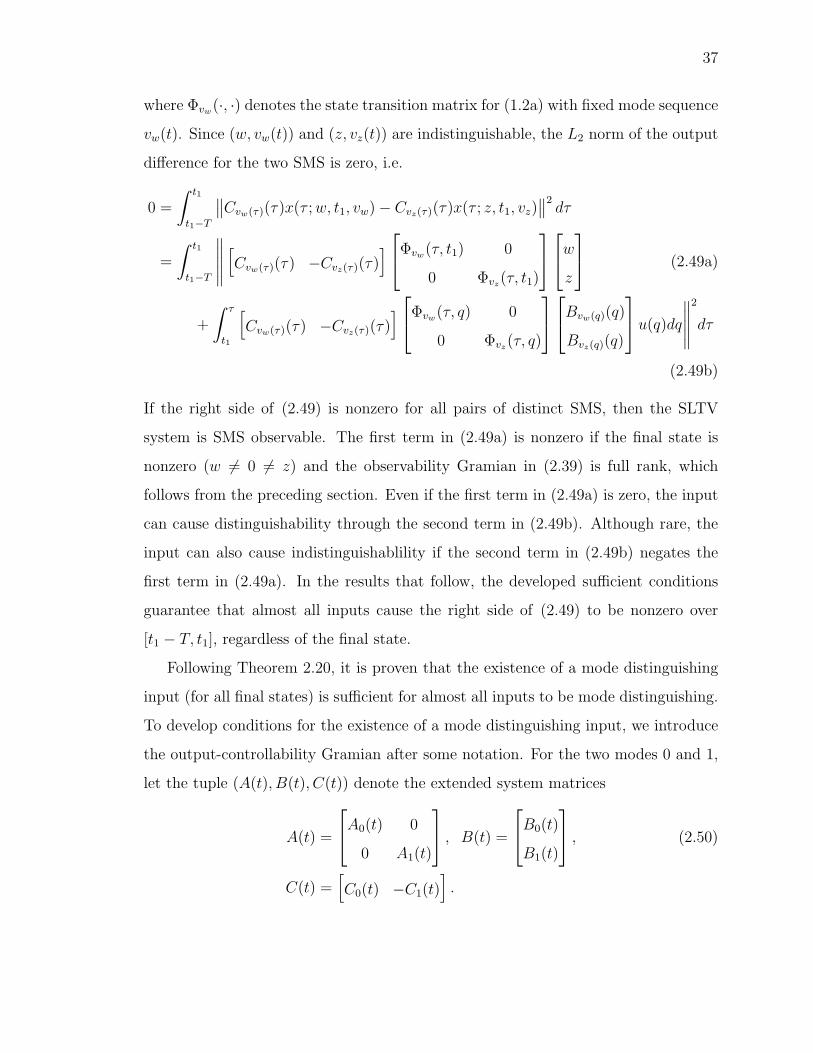
If the right side of (2.49) is nonzero for all pairs of distinct SMS, then the SLTV

system is SMS observable. The first term in (2.49a) is nonzero if the final state is

nonzero (w = 0 = z) and the observability Gramian in (2.39) is full rank, which

follows from the preceding section. Even if the first term in (2.49a) is zero, the input

can cause distinguishability through the second term in (2.49b). Although rare, the

input can also cause indistinguishablility if the second term in (2.49b) negates the

first term in (2.49a). In the results that follow, the developed sufficient conditions

guarantee that almost all inputs cause the right side of (2.49) to be nonzero over

[t1 − T, t1], regardless of the final state.

Following Theorem 2.20, it is proven that the existence of a mode distinguishing

input (for all final states) is sufficient for almost all inputs to be mode distinguishing.

To develop conditions for the existence of a mode distinguishing input, we introduce

the output-controllability Gramian after some notation. For the two modes 0 and 1,

let the tuple (A(t), B(t), C(t)) denote the extended system matrices

A(t) =

⎡⎣A0(t) 0

0 A1(t)

⎤⎦ , B(t) =

⎡⎣B0(t)

B1(t)

⎤⎦ , (2.50)

C(t) =[C0(t) −C1(t)

].

38

Introduced in [21], the output-controllability Gramian (OCG) for the extended system

is

P (t1 − T, t1) �∫ t1

t1−T

C(t1)Φ(t1, τ)B(τ)(C(t1)Φ(t1, τ)B(τ))�dτ (2.51)

For LTV systems, [21] proves that the OCG having full row rank is necessary and

sufficient for output controllability, i.e. for the existence on an input driving the out-

put to a specified value. For SLTV systems, we prove, in the following theorem, that

a nonzero extended OCG and positive definite extended observability Gramian over

each subinterval is sufficient for driving the extended system to a nonzero output, i.e.

sufficient for mode distinguishability. The following technical lemma develops the key

building block for proving the existence of an input causing mode distinguishability.

Lemma 2.19. Consider the two mode SLTV system Σ in (1.2) with a minimum

dwell time, Assumption 1.2. Consider two final state and mode sequences {w, vw}and {z, vz} such that over the subinterval [s1, s2) ⊂ (t1−T, t1), vw and vz are constant

and vw(t) = vz(t). If over every nonempty subinterval, [t′1, t′2] ⊂ [t1 − T, t1]

(i) WO(t′1, t

′2) > 0 and

(ii) P (t′1, t′2) = 0,

then there exists an input u(·) distinguishing {w, vw} and {z, vz}.

Proof. Without loss of generality, let vw(t) = 0 and vz(t) = 1 for all t ∈ [s1, s2). Since

P (s1, s2) = 0, there exists um ∈ Rm such that P (s1, s2)um = 0. We claim the input

u(t) =

⎧⎪⎨⎪⎩(C(s2)Φ(s2, t)B(t))�um, t ∈ [s1, s2)

0, otherwise

(2.52)

distinguishes {w, vw} and {z, vz}. Since over the interval [t1 − T, s1), u(t) = 0 and

WO(t1 − T, s1) > 0, Theorem 2.17 implies {w, vw} and {z, vz} are indistinguishable

only if the corresponding state trajectories xw and xz are zero at s1. We now consider

39

the case when xw(s1) = xz(s1) = 0. Let yw(t) and yz(t) denote the outputs of {w, vw}and {z, vz}, respectively. Then

yw(s2)− yz(s2) =

∫ s2

s1

C(s2)Φ(s2, τ)B(τ)u(τ)dτ

= P (s1, s2)um = 0.

implying {w, vw} and {z, vz} are distinguishable.

When all switching times are in A, Lemma 2.19 allows one to construct a mode

disinguishing input for all final states, as per the following theorem.

Theorem 2.20. Consider the two mode SLTV system Σ in (1.2) with a minimum

dwell time and all switching times in A, Assumptions 1.2 and 2.1, respectively. If

over every nonempty subinterval, [t′1, t′2] ⊂ [t1 − T, t1]

(i) WO(t′1, t

′2) > 0 and

(ii) P (t′1, t′2) = 0,

then there exists a mode distinguishing input u(t) for all final states over interval

[t1 − T, t1] .

Proof. The proof will proceed by considering separately each subinterval [si, si+1) with

si, si+1 ∈ A. For the subinterval [s0, s1), fix a time tm ∈ (s0, s1) and let u(t) = 0 on

the interval [s0, tm). Since there are no switching times in [tm, s1), Lemma 2.19 implies

the existence of a mode distinguishing input over [s0, s1) for all states at s1. Repeating

this construction over each interval [si, si+1) results in a mode distinguishing input

u(t) over [t1 − T, t1] for all final states, i.e. all final states at t1.

We now prove that the existence of an input distinguishing two subsystems for all

final states implies mode distinguishability for generic inputs. We assume that the

switching times are observable or contained in the known set A. Because potential

switching times are known, we need only prove generic mode distinguishability over

an interval [s1, s2) without switching. For the interval [s1, s2), let the set of inputs

40

not causing mode distinguishability for all final states be denoted Ui, a subset of the

entire input space Uf = LP (Rm). Recall that proving Ui is a proper subspace of Uf

implies that Ui has measure zero in Uf = Lp(Rm).

First we prove Ui is a subspace. For each u ∈ Ui, i.e. each input not mode distin-

guishing, there exists an extended final state xf causing the output of the extended

system to be zero over [s1, s2), an interval without switching. Consider u, u′ ∈ Ui with

the extended final states xf , x′f ∈ R

2n, respectively, which cause the output of the

extended system to be identically zero over [s1, s2). Then y(t; xf , u) = y(t; x′f , u′) = 0

for all t ∈ [s2, s2). Since the extended system is linear, superposition implies that for

all α, β ∈ R

y(t;αxf + βx′f , αu+ βu′) = αy(t; xf , u) + βy(t; x′f , u′)

= 0.

Thus αu+ βu′ ∈ Ui implying Ui is a subspace of Uf .

Given the conditions of Theorem 2.20 are satisfied, there exists a mode distin-

guishing input, i.e. an input u ∈ Ui. Thus Ui is a proper subspace and has Lebesgue

measure zero in Uf , i.e. mode distinguishability holds for generic (almost all) inputs.

With the mode observable, only state reconstruction remains, i.e. the classi-

cal LTV observability problem. Since the positive definite extended observability

Gramian implies observability of each LTV subsystem, the conditions in Theorem 2.20

are sufficient for SMS observability of SLTV systems as per the following theorem.

Theorem 2.21. Consider the two mode SLTV system Σ in (1.2) with a minimum

dwell time and all switching times in A, Assumptions 1.2 and 2.1. If over every

nonempty subinterval, [t′1, t′2] ⊂ [t1 − T, t1],

(i) WO(t′1, t

′2) < 0

(ii) P (t′1, t′2) = 0,

then Σ is SMS observable for almost all inputs.

41

Proof. By Assumptions 1.2 and 2.1, there are a finite number of intervals [si, si+1) ⊂[t1 − T, t1] without mode switches which partition [t1 − T, t1]. Over each interval

[si, si+1) without switching, Theorem 2.20 implies there exists and input causing mode

distinguishability. This implies that the mode sequence is observable for almost all

inputs. All that remains is to determine the final state. Since WO(t′1, t

′2) > 0, each

mode (active mode) has a positive definite observability Gramian over [t′1, t′2], i.e. the

state is observable over [t′1, t′2]. Thus the state x(t) is observable in each subinterval

[si, si+1) implying Σ is SMS observable for generic inputs.

2.4.3 Extensions to Nonlinear Switched Systems

In this section we extend results in Section 2.4.1 to switched nonlinear systems

without input and make a connection to the strong observability condition in [22].

Specifically, we consider two-mode switched nonlinear systems of the form

x = fv(t)(t, x) (2.53a)

y = gv(t)(t, x) (2.53b)

which satisfy the following assumptions:

(i) v(·) has a minimum dwell time,

(ii) there exists a unique solution to (2.53a) for each initial (final) condition x0 ∈ Rn

and any admissible mode sequence v(t),

(iii) fi(·, 0) = 0 and gi(·, 0) = 0 for all modes i ∈ {0, 1}.

As with the case for SLTV systems without input, we begin by considering when

switching times are observable. In Lemma 2.16, switching times for SLTV systems

without input are observable if the final state is nonzero and the observability Gramian

is positive definite over each nontrivial subinterval. The observability Gramian is not

defined for nonlinear systems; so a suitable nonlinear analog is desired. The following

lemma extends Lemma 2.16 after some notation. Let the output (2.53b) due to the

final state x at t1 and mode sequence v ≡ i be denoted yi(τ ; x, t1).

42

Lemma 2.22. Let Σ be a nonlinear switched system in (2.53). Consider an interval

[t1−T, t1] such that the final state is nonzero. If for any nontrivial subinterval [t′1, t′2]

and for all nonzero x, x ∈ Rn there exists γm = γm(t

′1, t

′2) > 0 such that

∫ t′2

t′1

‖y0(τ ; x, t′2)− y1(τ ; x, t2)‖2dτ ≥ γm

∥∥∥∥∥∥⎡⎣xx

⎤⎦∥∥∥∥∥∥2

, (2.54)

then Σ is switching time observable over [t1 − T, t1].

Note that (2.54) has the same effect as a positive definite extended observability

Gramian. Specifically, if the system in (2.53) were linear, then

∫ t′2

t′1

‖y0(τ ; x, t′2)− y1(τ ; x, t2)‖2dτ =

⎡⎣xx

⎤⎦�

WO(t′1, t

′2)

⎡⎣xx

⎤⎦≥ λmin(WO(t

′1, t

′2))

∥∥∥∥∥∥⎡⎣xx

⎤⎦∥∥∥∥∥∥2

.

With this observation, the proof of Lemma 2.22 follows Lemma 2.16.

With switching times observable, the main extension of Theorem 2.18 can be

introduced as per the following theorem.

Theorem 2.23. Let Σ be a nonlinear switched system in (2.53). Consider an interval

[t1−T, t1] such that the final state is nonzero. If for any nontrivial subinterval [t′1, t′2]

and for all final states x, x ∈ Rn there exists γm = γm(t

′1, t

′2) > 0 and γx = γx(t

′1, t

′2) >

0 such that

∫ t′2

t′1

‖y0(τ ; x, t′2)− y1(τ ; x, t2)‖2dτ ≥ γm

∥∥∥∥∥∥⎡⎣xx

⎤⎦∥∥∥∥∥∥2

, (2.55)

and for each mode i ∈ {0, 1}∫ t′2

t′1

‖yi(τ ; x, t′2)− yi(τ ; x, t′2)‖2dτ ≥ γx ‖x− x‖2 (2.56)

then Σ is SMS observable over [t1 − T, t1].

43

Satisfying (2.55) implies mode distinguishability over intervals without switching.

The minimum dwell time assumption guarantees that the interval [t1 − T, t1] can be

partitioned into a finite set of intervals [t′1, t2) without switching. Thus, the mode

sequence is observable. What remains is to guarantee feasibility of state reconstruc-

tion.

The condition in (2.56) is the strong state observability condition in [22]. The

strong observability condition guarantees the state is observable for each subsystem. If

the system in (2.53) is linear then lettingW iO(t

′1, t

′2) denote the observability Gramian

for mode i, ∫ t′2

t′1

‖yi(τ ; x, t′2)− yi(τ ; x, t′2)‖2dτ = (x− x)�W i

O(t′1, t

′2)(x− x)

≥ λmin(WiO(t

′1, t

′2))‖x− x‖2.

So (2.56) reduces to the observability Gramian in each mode being positive definite

if the system is linear. Hence, the state is observable if (2.56) is satisfied. Com-

bining state observability of each subsystem with the mode sequence observability

guaranteed by condition (2.55) proves Theorem 2.23.

2.4.4 Conclusions

This section extends the existing observability conditions for LTI switched systems

to those for LTV switched systems with and without input. Using the notion of

strong observability, sufficient conditions for observability of nonlinear switched state

models are also set forth, and represent a basis for continued research. The next

chapter explores a robustness metric for state and mode sequence observability for

SLTI systems with additive perturbations to each of the system matrices.

2.5 Appendix for Section 2.3

Lemma 2.14.

44

Proof. Let Σ = {A, C} be an LTI system

˙x(t) = Ax

y = Cx

where

A =

⎡⎣Av(t′) 0

0 Av(t′)

⎤⎦ , C =[Cv(t′) −Cv(t′)

]By calculation, Σ has observability matrix O = [O2n(v(t

′)),−O2n(v(t′))]. Thus, Σ

has an identically zero output for t ≥ t′ exactly when x(t′) ∈ Null(O) since Null(O)

is exactly the unobservable subspace for Σ. Defining x(t′) = [x(t′)T , x(t′)T ]T , the

preceding sentence can be expressed as

0 = Y∞(t′) = Y∞(t′)− Y∞(t′)

if and only if

[O2n(v(t′)),−O2n(v(t

′))]

⎡⎣x(t′)x(t′)

⎤⎦by the Cayley-Hamilton theorem proving the result.

Theorem 2.15.

Proof. For sufficiency assume that Σ is ST unobservable, each pair (Ci, Ai) is observ-

able for i ∈ SM , and (2.36) is satisfied. Since Σ is ST unobservable, there exists indis-

tinguishable SMS {x0, v(t)} and {x0, v(t)} with x0 or x0 nonzero, v(t0), v(t0) ∈ SM ,

and a switching time t1 such that v(t−1 ), v(t+1 ), v(t

−1 ) ∈ SM and v(t+1 ) ∈ FM . By the

definition of indistinguishable SMS

Y∞(t−1 ) = Y∞(t−1 ) (2.57a)

Y∞(t+1 ) = Y∞(t+1 ) (2.57b)

Define ks1 = v(t−1 ), ks2 = v(t+1 ), ks3 = v(t−1 ), and kf = v(t+1 ). Since by assumption

there are no state jumps at the transition, (2.57) and lemma 2.14 imply that⎡⎣O2n(ks1) O2n(ks3)

O2n(ks2) O2n(kf )

⎤⎦⎡⎣ x(t1)

−x(t1)

⎤⎦ = 0 (2.58)

45

The contradiction of (2.36) is nearly achieved. Equation (2.58) differs from (2.36)

only by the condition that ks1 = ks2 in (2.36). So if v(t−1 ) = v(t+1 ) then (2.36) is

contradicted and sufficiency follows.

On the other hand if ks1 = v(t−1 ) = v(t+1 ) = ks2, the output at t1 is smooth, i.e.

Y∞(t−1 ) = Y∞(t+1 ) (2.59)

Combining (2.59) with (2.57) we observe

Y∞(t−1 ) = Y∞(t+1 ) (2.60)

After substitution and manipulation, the first 2np rows of (2.60) imply

[O2n(v(t

−1 )) O2n(v(t

+1 ))

]⎡⎣ x(t1)

−x(t1)

⎤⎦ = 0 (2.61)

Then we must show that there is another combination of modes which contradicts

the ”for all” statement in (2.36).

Since both x0 and x0 cannot both be zero we can assume without loss of generality

x(t1) = 0 (due to the nonsingularity of the state transition matrix for the switched

LTI system).

To contradict the ”for all” statement in (2.36) we assign k′s2 = v(t−1 ) and k′f =

v(t+1 ). Now let k′s1 ∈ SM be a safe mode such that k′s1 = k′s2. Assign k′s3 = k′s1.

Combining these assignments with (2.61) results in⎡⎣O2n(k′s1) O2n(k

′s3)

O2n(k′s2) O2n(k

′f )

⎤⎦⎡⎣ x(t1)

−x(t1)

⎤⎦ = 0 (2.62)

providing the needed contradiction for sufficiency.

For the necessity of (Ci, Ai) observable for i ∈ SM , assume there exists ks ∈ SM

such that (Cks , Aks) is not observable. Then there exists nonzero x ∈ Rn such that

O2n(ks)x = 0. Consider the two SMS {x0 = x, v(t) = ks ∀t} and {x0 = 0, v(t)} where

v(t) is

v(t) =

⎧⎪⎨⎪⎩ks, if t ≤ t1

kf , if t > t1

46

and t1 ∈ (t0, tf ). Then {x0, v(t)} and {x0, v(t)} produce outputs y(t) = y(t) ≡ 0,

which contradicts that Σ is ST observable.

For necessity of (2.36), assume (2.36) is not satisfied. Thus there exists integers

ks1 = ks2, ks3 ∈ SM , kf ∈ FM such that

rank

⎡⎣O2n(ks1) O2n(ks3)

O2n(ks2) O2n(kf )

⎤⎦ = rank[M ] ≤ 2n (2.63)

Thus there exists a nonzero z ∈ R2n such that Mz = 0. Defining z = [xT1 ,−xT1 ]

implies that x1 or x1 is nonzero (or both) and

⎡⎣O2n(ks1) O2n(ks3)

O2n(ks2) O2n(kf )

⎤⎦⎡⎣ x1

−x1

⎤⎦ = 0 (2.64)

This half of the proof will proceed by constructing two indistinguishible SMS

based on (2.64) which will imply Σ is ST unobservable. First consider t1 to be a time

in (t0, tf ) and define two mode sequences as

v(t) =

⎧⎪⎨⎪⎩ks1, if t ≤ t1

ks2, if t > t1

(2.65)

v(t) =

⎧⎪⎨⎪⎩ks3, if t ≤ t1

kf , if t > t1

Since for (2.65) there is only one switch at t1 in [t0, tf ) the initial states can be

constructed as

x0 = eAks1(t0−t1)x1

x0 = eAks3(t0−t1)x1

We can now construct the SMS {x0, v(t)} and {x0, v(t)}.

47

First consider the interval t ∈ [t0, t1]. Let Y2n(t) and Y2n(t) be the outputs and

2n− 1 derivatives of {x0, v(t)} and {x0, v(t)}, respectively. Then

Y2n(t)− Y2n(t) =[O2n(ks1) O2n(ks3)

]⎡⎣ eAks1(t−t1)x1

eAks3(t−t1)(−x1)

⎤⎦ (2.66)

If (2.66) is equal to zero for all t ∈ [t0, t1) then lemma 2.14 guarantees Y2n(t) = Y2n(t),

i.e. the outputs are identically equal. To prove (2.66) is equal to zero, we define a

new LTI system (C, A) where

C =[Cks1 Cks3

], A =

⎡⎣Aks1 0

0 Aks3

⎤⎦Note that the observability matrix of (C, A) is exactly the matrix

R =[O2n(ks1) O2n(ks3)

]in (2.66). From linear system theory, the null space of the observability matrix is A-

invariant. That is Ax ∈ Null(R) if x ∈ Null(R). By the Cayley-Hamilton theorem,

A satisfies its own differential equation and Ak for k ≥ 2n can be written as a linear

combination of lower powers of A. Since eAt =∑∞

j=0 1/j!Ajtj by definition, the

Cayley-Hamilton theorem combined with the A-invariance of R implies

0 =[O2n(ks1) O2n(ks3)

]eA(t−t1)

⎡⎣ x1

−x1

⎤⎦ (2.67)

=[O2n(ks1) O2n(ks3)

]⎡⎣ eAks1(t−t1)x1

eAks3(t−t1)(−x1)

⎤⎦By (2.66) and (2.67), lemma 2.14 implies that the outputs of {x0, v(t)} and

{x0, v(t)} are identically equal over [t0, t1]. By the same argument, it can be shown

that the outputs are identically equal over the interval (t1, tf ). Thus {x0, v(t)} and

{x0, v(t)} are indistinguishible implying Σ is ST unobservable completing the proof

of necessity.

48

3. STRUCTURED ROBUST PROPERTY METRIC:

P-ROBUSTNESS

3.1 Introduction

System properties, such as controllability and observability, are often characterized

by binary labels, e.g., controllable or uncontrollable and stable or unstable. These

binary labels fail to capture the robustness of these properties. For example, consider

the LTI system

x(t) = Ax(t) + Bu(t), (3.1)

where A ∈ Rn×n and B ∈ R

n×m. The pair (A,B) is controllable if and only if for

each λ ∈ C

rank[A− λIn B

]= n, (3.2)

where In denotes the n × n identity matrix [23]. The set of uncontrollable pairs

(A,B) ∈ Rn×(n+m), i.e., pairs failing to satisfy (3.2), is an algebraic variety of lower

dimension and hence has measure zero in Rn×(n+m). Since LTI models are only ap-

proximations of physical systems, it is also necessary to characterize the robustness

of the controllability property, e.g., by determining the distance to the nearest un-

controllable system [24,25]

μR(A,B) = inf(δA,δB)∈C

‖[δA, δB]‖F , (3.3)

where C = {(δA, δB) : ∃λ ∈ C, rank[A − δA − λIn, B − δB] < n}. Similar metrics

can be constructed for system properties including, but not limited to reachability,

stabilizability, observability, and detectability.

Computing metrics such as μR(A,B) and the associated minimizing perturbations

has been an active area of research over the past 40 years [24–37]. The norm used to

measure robustness separates the robust system property literature. The Frobenius

49

norm metric in (3.3) is based on the work of [24] and is used in [25–31]. The primary

alternative to the Frobenius norm metric is the spectral norm, i.e., the largest singular

value of the matrix [δA, δB]. The spectral norm metric, usually referred to by the

names controllability radius or observability radius, is explored in several works in-

cluding [31–36]. This paper utilizes a Frobenius norm metric because a perturbation

on each entry of a system matrix affects the Frobenius norm in a strong and direct

way.

The primary challenge to either robustness metric is developing an algorithm to

compute the minimum distance and associated perturbation matrices. In [25], the

algorithm for computing (3.3) for real but otherwise unstructured perturbations is

based on computing a coordinate transformation into a “nearly” Kalman uncontrol-

lable form. Another approach for computing (3.3) is considered in [29] wherein one

constructs a large n(n + 1) × n(n + m) matrix Xn−1 consisting of a structured ar-

rangement of blocks of matrices ⎡⎣A B

I 0

⎤⎦ .The “Structured Total Least Norm” algorithm then computes a low rank approxi-

mation to Xn−1 where only the A and B matrices are potentially perturbed. The

low rank approximation also provides the smallest perturbations δA ∈ Rn×n and

δB ∈ Rn×m causing uncontrollability.

Reference [32] develops an algorithm for computing the controllability radius for

real but otherwise unstructured perturbations utilizing a constrained optimization

problem; the perturbations causing uncontrollability are constructed from singular

vectors. In [36], a fast algorithm for computing the controllability radius is developed

for unstructured complex perturbations. Extensions to higher-order LTI systems with

affine perturbations are considered in [33]. Additional extensions including descriptor

and time-delay LTI systems are considered in [34]. Finally, [31] develops an upper

bound on the spectral distance to uncontrollability of a switched LTI system.

50

Reference [38] formulates the problem of structured rank reducing perturbations,

belonging to a subspace S ⊂ Cn×m, on a rectangular matrix M ∈ C

n×m which

cause the failure of a system property, P , such as controllability, observability, or

stability. This general P–robustness framework encompasses many of the robustness

problems previously addressed in the literature. No prior work has extended the

P–robustness framework, proven the necessary conditions for P–robustness, or com-

pleted and proven convergence of the algorithm suggested in [38]; this list constitutes

the main contributions of the current paper.

Section 3.2 introduces the P–robustness framework. Section 3.3 establishes neces-

sary conditions for solving the P–robustness problem. The necessary conditions mo-

tivate an algorithm for solving the P–robustness problem introduced in Section 3.4.

The algorithm converges to a point satisfying the necessary conditions and is demon-

strated with numerical examples in Section 3.6.

In this paper, the following notation will be used:

||M ||F Frobenius norm of a matrix M .

||ν||2 Euclidean norm of a vector ν.

M�, MH Transpose and conj. transpose of M .

σn(M) nth singular value of matrix M .

Im m×m identity matrix.

diag(ν) Diag. matrix with diag. entries in ν.

vec(M) Vectorizes M by stacking the columns.

M ⊗N The kronecker product of M and N .

M † The Moore-Penrose pseudoinverse.

Im(M) Imag. component of M .

Re(M) Real component of M .

σi(M) ith largest singular value of M .

cl(U) The closure of the set U .

〈A1, A2〉 Inner product of A1, A2 ∈ Cn×m defined as 〈A1, A2〉 =

Re(vec(A1))� Re(vec(A2)) + Im(vec(A1))

� Im(vec(A2))

51

3.2 P-Robustness Problem

This section specifies the details of the P–robustness problem. Later sections

restate and rigorously prove necessary conditions for its solution (Theorem 3.2) and

develop a complete algorithm (Algorithm 1) that converges to a point satisfying those

necessary conditions, under appropriate assumptions.

Definition 3.1. [38] Let M ∈ Cn×m with n ≤ m (without loss of generality); let

P ⊂ Cn×m and S ⊂ C

n×m be linear spaces over R. The P–robustness of M with

respect to parameter variations in S is defined as

r(M ;S,P) = infδM∈T

‖δM‖F (3.4)

where

T = {δM ∈ S : ∃R ∈ P , rank[M − δM −R] < n} (3.5)

As mentioned, the Frobenius norm metric, used herein, directly measures the mag-

nitude of the parameter variations and thus appears to more accurately represent

the robustness of the system property. This is in contrast to the controllability (and

observability) radius which measures the largest singular value of the perturbation

causing uncontrollability (unobservability), a metric that may not reflect some pa-

rameter variations: for a fixed largest singular value, changes in the smaller singular

values due to parameter variations go unnoticed.

It is useful to consider bases for S and P (which are linear subspaces over the

field R). Let {S1, S2, · · · , Sk} be an orthonormal basis for S and {P1, P2, · · · , Pr}be an orthonormal basis for P , where by orthonormal we mean that 〈Si, Sj〉 �Re(vec(Si))

� Re(vec(Sj)) + Im(vec(Si))� Im(vec(Sj)) is 0 if i = j and 1 if i = j.

Each perturbation δM ∈ S can be represented by an associated vector ζ ∈ Rk in this

basis {S1, S2, · · · , Sk}, i.e., δM =∑k

i=1 ζiSi. Similarly, each R ∈ P is represented

by a vector ρ ∈ Rr. Using the fixed bases for S and P , we can reformulate the

P–robustness of M with respect to perturbations in S.

52

Definition 3.2. Let M ∈ Cn×m; let P ⊂ C

n×m and S ⊂ Cn×m be linear spaces over

R with orthonormal bases {S1, S2, · · · , Sk} and {P1, P2, · · · , Pr}, respectively. The

P–robustness of M with respect to parameter variations in S is

r(M ;S,P) = infζ∈Rk, ρ∈Rr

‖ζ‖2 (3.6)

subject to:

0 = σn

(M −

k∑i=1

ζiSi −r∑

j=1

ρjPj

)� H(ζ, ρ). (3.7)

Note, Definition 3.2 is equivalent to Definition 3.1. Also, the P–robustness of M

with respect to parameter variations in S is independent of the orthonormal basis.

Of course, the representation of the minimizing pair (ζ∗, ρ∗) depends on the selected

bases for S and P .

For use later in the paper, we define

f(ζ, ρ) = 0.5‖ζ‖22. (3.8)

A minimizer (ζ∗, ρ∗) to (3.6) subject to (3.7) (when it exists) is the same when ‖ζ‖2is replaced by f(ζ, ρ) in (3.6). The function f(ζ, ρ) is preferable because it simplifies

the proofs later in the paper.

Example 3.1. Applying the P–robustness formulation to controllability of an LTI

state model (A,B,C), we set M = [A,B], R = [λI, 0], and δM = [δA, δB], where

δM has a specific perturbation structure defined by a basis for S.

The original motivation for this work stems from the need for specific structured

real perturbations for the state and mode sequence (SMS) observability problem of

switched LTI (SLTI) systems with safety applications described in [20, 30]. SMS

observability of SLTI systems can also be formulated as a P–robustness problem:

Example 3.2. For the problem of computing the distance to the nearest SMS unob-

servable SLTI system (which can model transitions from safe to unsafe operation), the

53

P–robustness framework can be applied to each pair of modes i (safe) and j (unsafe)

by defining

Mij =

⎡⎣A�i 0 C�

i

0 A�j C�

j

⎤⎦ ∈ R2n×(2n+p)

δMij = −

⎡⎣δA�i 0 δC�

i

0 δA�j δC�

j

⎤⎦ ∈ R2n×(2n+p)

R =

⎡⎣λI 0 0

0 λI 0

⎤⎦ ∈ C2n×(2n+p).

Clearly, the perturbation δMij has a specialized structure that is problematic for most

existing approaches. The P–robustness of Mij with respect to parameter variations

δMij ∈ S provides rij � r(Mij,S,P), see (3.4). Then mini,j{rij} is exactly the

distance to the nearest SMS unobservable SLTI system.

The rank reduction in the P–robustness problem is characterized by the nth sin-

gular value of M − δM − R becoming zero. To analyze the nth singular value, we

define the following linear operator:

Definition 3.3. Each pair of matrices u ∈ Cn and V ∈ C

m×(m−n+1) induces a linear

operator LuV : Cn×m → C1×(m−n+1) given by

LuV (N) = uHNV. (3.9)

Proposition 3.1. Let N = UΣV H be the singular value decomposition of N . Define

u to be the last column of U and V to be the last m− n+ 1 columns of V . Then

LuV (N) =[σn(N) 0 · · · 0

].

Consequently, ‖LuV (N)‖F = σn(N).

The linear operator LuV is defined for any u and V , independent of the argument.

For example, u and V can be related to the singular value decomposition of a matrix

M − δM − R and operate on any matrix N ′ ∈ Cn×m. Since the perturbations

and property matrices belong to lower dimensional subspaces S and P , we define

additional linear operators that have domains restricted to these subspaces.

54

Definition 3.4. For u ∈ Cn and V ∈ C

m×(m−n+1), the linear operators LuV S : S →C

1×(m−n+1) and LuV P : P → C1×(m−n+1) are defined as

LuV S(δM) � LuV |S(δM) = uHδMV

LuV P(R) � LuV |P(R) = uHRV.

The distinctions of the operator domains are pertinent when considering the pseu-

doinverses L†uV S : C1×(m−n+1) → S and L†

uV P : C1×(m−n+1) → P . The map LuV S is

surjective if for each y ∈ C1×(m−n+1) there exists δM ∈ S such that LuV S(δM) = y.

When LuV S is surjective, the pseudoinverse map L†uV S(y) = δM is the smallest matrix

δM ∈ S (in the Frobenius norm sense) solving the equation LuV S(δM) = y.

Fundamental to the solution of the P–robustness problem is the surjectivity of a

family of maps {LuV S} as per the following assumption:

Assumption 3.1. Let δM ∈ S and R ∈ P. Let M − δM − R have singular value

decomposition UΣV H . Define u to be the nth column of U and V to be the last

m − n + 1 columns of V . Then we assume LuV S is surjective for each δM ∈ S and

every R ∈ P.

We would like to explain why Assumption 3.1 is appropriate. Using Kronecker prod-

uct notation, LuV S is surjective if and only if

rank

⎡⎣Re [(V � ⊗ uH)BS]

Im[(V � ⊗ uH)BS

]⎤⎦ = 2(m− n+ 1). (3.10)

where {S1, · · · , Sk} is a basis for S and BS � [vec(S1), · · · , vec(Sk)]. Clearly, BS

must have at least 2(m− n+ 1) columns for (3.10) to be satisfied, i.e., S as a vector

space over R must have dimension no less than 2(m− n + 1). Consequently, for the

problem to be solvable, we require that the perturbation space S be sufficiently rich.

The proof of (3.10) and related surjectivity results are included in the appendix.

As described in [38], the surjectivity of LuV S ensures a certain regularity condition

on a rank reducing perturbation/property matrix pair (δM,R) ∈ S × P . This regu-

larity condition guarantees that there are neighboring perturbation/property matrix

55

pairs (δM ′, R′) which are also rank reducing, i.e., δM is not an isolated rank reducing

perturbation.

If a rank reducing perturbation is isolated it is naturally a local minimum. A P–

robustness problem with a finite number of isolated extrema is much easier to solve:

one can find ζ ∈ Rk and ρ ∈ R

r such that det[M(ζ, ρ)M(ζ, ρ)�] = 0, where

M(ζ, ρ) =M −k∑

i=1

ζiSi −r∑

i=1

ρiPi. (3.11)

Consequently, we focus on P–robustness problems satisfying the surjectivity assump-

tion. In addition, we can exclude P–robustness problems where rank(M − R) < n

for some R ∈ P (i.e., M does not satisfy the property P) since r(M ;S,P) = 0

in this case. The next section sets up necessary conditions for the solution to the

P–robustness problem.

3.3 Necessary Conditions

The objective of this section is proving the necessary conditions on a minimum

norm rank-reducing perturbation δM∗ ∈ S and the associated property matrix R∗ ∈P (when they exist), i.e., ‖δM∗‖F = r(M ;S,P) and rank(M − δM∗ − R∗) < n. We

next provide some intuition for the necessary conditions.

Let us first assume that the property matrix R∗ is fixed. For δM∗ to be the

minimum norm rank-reducing perturbation for M − R∗, the tangent plane to the

hypersurface Υ1 = {δM ∈ S : σn(M − R∗ − δM) = 0} must be perpendicular to

the line connecting M − R∗ and M − R∗ − δM∗, see Figure 3.1. For u∗ the nth left

singular vector (lsv) and V∗ having columns equal to the nth throughmth right singular

vectors (rsv) of M −R∗ − δM∗, ‖Lu∗V∗(M −R∗ − δM∗)‖F = σn(M −R∗ − δM∗) = 0.

As will be seen in the proof of Theorem 3.2, the hyperplane Υ2 = {δM ∈ S :

Lu∗V∗(M−R∗−δM) = 0} is related to the tangent plane to Υ1 at δM∗. Note, elements

of Υ2 are precisely the minima of ‖Lu∗V∗S(δM)− Lu∗V∗(M − R∗)‖F over δM ∈ S. IfδM∗ is the smallest rank reducing perturbation onM−R∗, then δM∗ has the smallest

norm of any perturbation in Υ2, i.e., δM∗ minimizes ‖Lu∗V∗S(δM∗)−Lu∗V∗(M−R∗)‖F

56

and ‖δM∗‖F has the least norm of all such matrices. Since Lu∗V∗S is surjective by

Assumption 3.1, the minimum is given by

δM∗ = (L†u∗V∗S ◦ Lu∗V∗)(M −R∗), (3.12)

the first necessary condition in Theorem 3.2.

The second necessary condition addresses the locally optimal property matrix R∗.

As per the discussion above, the optimal rank reducing perturbation satisfies (3.12).

Let ΔR ∈ P be an alteration to R∗. Define

δM0(ΔR) � (L†u0V0S ◦ Lu0V0)(M −R∗ −ΔR) (3.13)

where u0 is the nth lsv and V0 has columns equal to the nth through mth rsv of

M − R∗ − ΔR − δM0(ΔR). It is difficult to directly minimize the norm of (3.13)

with respect to ΔR because the matrices u0 and V0 change with ΔR. However, for

sufficiently small ΔR, we will approximate δM0(ΔR) with

δM0(ΔR) ≈ (L†u∗V∗S ◦ Lu∗V∗)(M −R∗ −ΔR), (3.14)

where u∗ is the nth lsv and V∗ has columns equal to the nth through mth rsv of

M−R∗−δM∗. Thus in a sufficiently small neighborhood of R∗, minimizing the norm

of (3.13) with respect to ΔR is equivalent to minimizing

‖(L†u∗V∗S ◦ Lu∗V∗P)ΔR− (L†

u∗V∗S ◦ Lu∗V∗)(M −R∗)‖F . (3.15)

The least square minimum of (3.15) is given by

ΔR = (L†u∗V∗S ◦ Lu∗V∗P)

†(L†u∗V∗S ◦ Lu∗V∗)(M −R∗). (3.16)

If R∗ is the optimal property matrix, then (3.15) is minimized at ΔR = 0. Hence,

the right-hand side of (3.16) equals zero, the second necessary condition.

Theorem 3.2. Suppose there exists δM∗ ∈ S that is a local minimum norm element

of the set T = {δM ∈ S : ∃R ∈ P , rank[M − δM − R] < n}; choose R∗ ∈ {R ∈ P :

rank[M − δM∗−R] < n} and let u be a non-trivial element of ker[(M − δM∗−R∗)H ]

and let V be a matrix whose columns span ker[M − δM∗ −R∗]. If LuV S is surjective,

then the following two necessary conditions both hold:

58

1a) δM∗ ∈ S is a minimum norm matrix minimizing

‖LuV S(δM∗)− LuV (M −R∗)‖F .

2a) 0 = ΔR∗, where ΔR∗ ∈ P is the minimum norm matrix minimizing

‖(L†uV S ◦ LuV P)(ΔR∗)− (L†

uV S ◦ LuV )(M −R∗)‖F .

Equivalently,

1b) δM∗ = (L†uV S ◦ LuV )(M −R∗) and

2b) 0 = ΔR∗ = (L†uV S ◦ LuV P)

†(L†uV S ◦ LuV )(M −R∗).

Remark 3.1. Conditions 1a and 2a could be generalized to other norms, such as the

spectral norm. On the other hand, conditions 1b and 2b are Frobenius-norm specific.

Note, condition 1a essentially requires δM∗ to be the smallest matrix minimizing

σn(M − R∗ − δM) for δM ∈ S. So even when no rank reducing perturbation exists,

condition 1a provides the “best” solution.

The proof of Theorem 3.2 requires some machinery and four technical lemmas. As

will be seen, proving the necessary conditions in Theorem 3.2 requires the application

of the inverse function theorem1 which in turn requires Frechet differentiability of the

equality constraint H(ζ, ρ) = 0 in (3.7). Unfortunately, there are points at which H

is only directionally differentiable. These non-Frechet differentiable points are caused

by two structural components of the svd: i) the ordering of the singular values and

ii) the requirement that the singular values be positive. We observe that, in general,

perturbation and property matrices δM and R for whichM − δM −R has a repeated

smallest singular value or a zero smallest singular value is an algebraic variety of lower

dimension in S×P . Consequently, the functionH(ζ, ρ) is Frechet differentiable almost

1A simpler proof of the necessary conditions which does not require the inverse function theoremcan be developed if the conditions in Proposition 3.16 (in the appendix) are satisfied. This simplerproof is consistent with the proof outlined in [38], but requires conditions stronger than surjectivity.

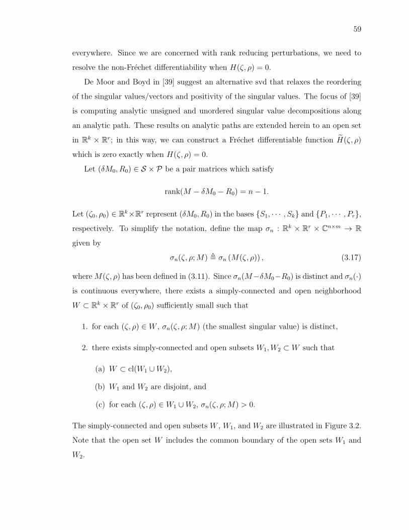
59

everywhere. Since we are concerned with rank reducing perturbations, we need to

resolve the non-Frechet differentiability when H(ζ, ρ) = 0.

De Moor and Boyd in [39] suggest an alternative svd that relaxes the reordering

of the singular values/vectors and positivity of the singular values. The focus of [39]

is computing analytic unsigned and unordered singular value decompositions along

an analytic path. These results on analytic paths are extended herein to an open set

in Rk × R

r; in this way, we can construct a Frechet differentiable function H(ζ, ρ)

which is zero exactly when H(ζ, ρ) = 0.

Let (δM0, R0) ∈ S × P be a pair matrices which satisfy

rank(M − δM0 −R0) = n− 1.

Let (ζ0, ρ0) ∈ Rk×R

r represent (δM0, R0) in the bases {S1, · · · , Sk} and {P1, · · · , Pr},respectively. To simplify the notation, define the map σn : Rk × R

r × Cn×m → R

given by

σn(ζ, ρ;M) � σn (M(ζ, ρ)) , (3.17)

whereM(ζ, ρ) has been defined in (3.11). Since σn(M−δM0−R0) is distinct and σn(·)is continuous everywhere, there exists a simply-connected and open neighborhood

W ⊂ Rk × R

r of (ζ0, ρ0) sufficiently small such that

1. for each (ζ, ρ) ∈ W , σn(ζ, ρ;M) (the smallest singular value) is distinct,

2. there exists simply-connected and open subsets W1,W2 ⊂ W such that

(a) W ⊂ cl(W1 ∪W2),

(b) W1 and W2 are disjoint, and

(c) for each (ζ, ρ) ∈ W1 ∪W2, σn(ζ, ρ;M) > 0.

The simply-connected and open subsets W , W1, and W2 are illustrated in Figure 3.2.

Note that the open set W includes the common boundary of the open sets W1 and

W2.

61

Let g : [0, 1] → W be an analytic function with g(s) ∈ W1 for s < 0.5 and

g(s) ∈ W2 for s > 0.5. According to [39, Theorem 1], there exists an analytic

function fg : [0, 1] → R, called the unsigned nth singular value function, such that

|fg(s)| = σn(g(s);M), s ∈ [0, 1].

The function fg can only change sign as it transitions through the common boundary

of W1 and W2, i.e., at s = 0.5. By [39, Theorem 3], there exists analytic singular

vector functions ug : [0, 1] → Cn and vg : [0, 1] → C

m such that for each s ∈ [0, 1],

ug(s) and vg(s) are the unsigned nth lsv and rsv associated with fg(s), i.e., ug(s) and

vg(s) are unit vectors satisfying

uHg (s)

(M −

k∑i=1

ζgi(s)Si −r∑

j=1

ρgj(s)Pj

)= fg(s)v

Hg (s),

for each s ∈ [0, 1], where ζg : [0, 1] → Rk and ρg(s) → R

r are defined by the relation

g � (ζg, ρg).

Let H : W → R be the extension of the unsigned singular value function fg to

the set W , i.e.,

H(ζ, ρ) =

⎧⎪⎨⎪⎩sign(fg(0))σn(ζ, ρ;M) (ζ, ρ) ∈ W1

sign(fg(1))σn(ζ, ρ;M) otherwise

. (3.18)

Note that, H(g(s)) = fg(s) for each s ∈ [0, 1] since by construction of g(s), fg

can change sign only at s = 0.5. In addition, the form of H implies that for each

(ζ, ρ) ∈ W , |H(ζ, ρ)| = σn(ζ, ρ). We will show that H is Frechet differentiable on W ,

as per the following lemma.

Lemma 3.3. Let (ζ0, ρ0) ∈ Rk×R

r satisfy rank[M(ζ0, ρ0)] = n−1. Let W ⊂ Rk×R

r

be as defined above. Let H : W → R be as in (3.18). Then H is Frechet differentiable

on W with partial derivatives given by

∂H(ζ, ρ)

∂ζi= −Re(uHSiv)

∂H(ζ, ρ)

∂ρi= −Re(uHPiv),

(3.19)

62

where u and v are unsigned nth lsv and rsv ofM(ζ0, ρ0), i.e., uHM(ζ0, ρ0) = H(ζ, ρ)vH

and M(ζ0, ρ0)v = H(ζ, ρ)u.

Proof. See appendix.

As per Lemma 3.3, we now consider replacing the equality constraint H(ζ, ρ) = 0

with H(ζ, ρ) = 0 on the set W . For each (ζ0, ρ0) ∈ W , H has Frechet derivative

H ′(ζ0, ρ0) given by

−Re[uHS1v, · · · , uHSkv, u

HP1v, · · · , uHPrv], (3.20)

where u and v are unsigned nth lsv and rsv of M − δM0 − R0 with δM0 ∈ S and

R0 ∈ P the matrices represented by ζ0 and ρ0, respectively.

The next lemma proves that if the condition 1a (or equivalently 1b) of Theorem 3.2

is not satisfied, then there exists a direction ΔM ∈ S to change the perturbation δM∗

on the tangent plane LuV (·) = 0 (see Figure 3.1). This new perturbation δM∗ +ΔM

may not be rank reducing, but will allow us to prove the existence of rank reducing

perturbations with norms smaller than ‖δM∗‖F .

Lemma 3.4. Let M ∈ Cn×m, δM0 ∈ S, R0 ∈ P satisfy rank[M−δM0−R0] < n with

LuV S surjective, where u is the nth lsv and V has columns equal to the nth through

mth rsv of M − δM0 −R0. Suppose δM0 = (L†uV S ◦LuV )(M −R0). Then there exists

a matrix ΔM ∈ S such that

LuV S(ΔM) = 0 (3.21)

and

〈δM0,ΔM〉 < 0. (3.22)

Proof. See appendix.

Similar to Lemma 3.4, the following lemma proves that if the second necessary

condition of Theorem 3.2 is not satisfied, then there exist directions ΔM and ΔR for

changing perturbation δM∗ and the property matrix R∗, respectively, reducing the

norm of the perturbation on the tangent surface LuV (·) = 0 . This will allow us to

63

prove to existence of a rank reducing perturbation with smaller norm (and associated

property matrix).

Lemma 3.5. Let M ∈ Cn×m, δM0 ∈ S, R0 ∈ P satisfy rank[M−δM0−R0] < n with

LuV S surjective, where u is the nth lsv and V has columns equal to the nth through

mth rsv of M − δM0 −R0. Suppose δM0 = (L†uV S ◦ LuV )(M −R0) and

0 = ΔR � (L†uV S ◦ LuV P)

†(L†uV S ◦ LuV )(M −R0).

Then there exist ΔM ∈ S such that

LuV (ΔM +ΔR) = 0 (3.23)

and

〈δM0,ΔM〉 < 0. (3.24)

Proof. See appendix.

The last technical lemma provides the machinery for using Lemma’s 3.4 and 3.5

to prove the existence of rank reducing perturbations with smaller Frobenius norm

given that one of the two necessary conditions is not satisfied.

Lemma 3.6. Let (ζ0, ρ0) ∈ Rk×R

r satisfy rank(M(ζ0, ρ0)) = n−1 and W ⊂ Rk×R

r

be a neighborhood of (ζ0, ρ0) as in Lemma 3.3 where the nth singular value is distinct.

Let T : W → R2 be the function

T (ζ, ρ) =

⎡⎣f(ζ, ρ)− f(ζ0, ρ0)

H(ζ, ρ)

⎤⎦ , (3.25)

where f and H are defined in (3.8) and Lemma 3.3, respectively. If i) ∂∂ζH(ζ, ρ0)|ζ=ζ0

is surjective and ii) there exists ρΔ ∈ Rr and ζΔ ∈ R

k such that ζ�0 ζΔ < 0 and

H ′(ζ0, ρ0)[ζ�Δ, ρ

�Δ]

� = 0, then T is Frechet differentiable and T ′(ζ0, ρ0) is surjective.

Proof. See appendix.

We can now prove necessary conditions as per the following proof.

64

Proof of Theorem 3.2.

Condition 1: For contradiction, assume that δM0 is a minimum norm element

in T (defined in (3.5)) with associated property matrix R0, but condition 1 is not

satisfied, i.e.,

δM0 = (L†uV S ◦ LuV )(M −R0) (3.26)

where u ∈ Cn and V ∈ C

m×(m−n+1) are the nth lsv and nth through mth rsv of M −δM0−R0, respectively. By Lemma 3.4, there exists ΔM ∈ S such that LuV S(ΔM) = 0

and 〈δM0,ΔM0〉 < 0. Let ζ0 and ζΔ in Rk represent δM0 and ΔM in the orthonormal

basis {S1, · · · , Sk}, respectively. Let ρ0 ∈ Rr represent R0 in the orthonormal basis

{P1, · · · , Pr}. Since the basis {S1, · · · , Sk} is orthonormal, ζ�0 ζΔ = 〈δM0,ΔM〉 < 0.

By the form of H ′(ζ0, ρ0) in Lemma 3.3,

H ′(ζ0, ρ0)

⎡⎣ζΔ0

⎤⎦ = −Re(uHΔMv),

where v is the nth unsigned rsv ofM−δM0−R0. Since LuV S(ΔM) = 0 and v is a linear

combination of the columns of V , uHΔMv = 0. This implies H ′(ζ0, ρ0)[ζ�Δ, 0]

� = 0.

In addition, since LuV S is surjective, then ∂∂ζH(ζ, ρ0)|ζ=ζ0 is also surjective. Hence by

Lemma 3.6, T (ζ, ρ) given in (3.25) is Frechet differentiable and T ′(ζ0, ρ0) is surjective.

Thus by the inverse function theorem [40], there exists an open setW ⊂ R2 containing

zero such that for all y ∈ W , there exists ζy ∈ Rk and ρy ∈ R

r such that T (ζy, ρy) = y.

Hence for all sufficiently small neighborhoods of 0 in R2, there exists δ > 0, ζ∗ ∈ R

k,

and ρ∗ ∈ Rr such that T (ζ∗, ρ∗) = [−δ, 0]�. This implies that δM∗ =

∑ki=1 ζ∗iSi ∈ T ,

i.e., a rank reducing perturbation, with associated property matrix R∗ =∑r

j=1 ρ∗jRj.

Since f(ζ∗, ρ∗)− f(ζ0, ρ0) = −δ < 0, ‖δM∗‖F < ‖δM0‖F contradicting that δM0 is a

local minimum norm element in T .

65

Condition 2: For contradiction, assume that δM0 is a minimum norm element

in T with associated property matrix R0 and condition 1 is satisfied, but condition 2

is not, i.e.,

δM0 = (L†uV S ◦ LuV )(M −R0), and (3.27)

0 = (L†uV S ◦ LuV P)

†(L†uV S ◦ LuV )(M −R0) (3.28)

where u ∈ Cn and V ∈ C

m×(m−n+1) are the nth lsv and nth through mth rsv of

M − δM0 − R0, respectively. By Lemma 3.5, there exists ΔM ∈ S and ΔR ∈ Psuch that LuV (ΔM +ΔR) = 0 and 〈δM0,ΔM0〉 < 0. Let ζ0 and ζΔ in R

k represent

δM0 and ΔM in the orthonormal basis {S1, · · · , Sk}, respectively. Let ρ0 and ρΔ

represent R0 and ΔR in the orthonormal basis {P1, · · · , Pr}, respectively. Since the

basis {S1, · · · , Sk} is orthonormal, ζ�0 ζΔ = 〈δM0,ΔM〉 < 0. By the form of H ′(ζ0, ρ0)

in Lemma 3.3,

H ′(ζ0, ρ0)

⎡⎣ζΔρΔ

⎤⎦ = −Re(uHΔMv).

Since LuV (ΔM+ΔR) = 0, uH(ΔM+ΔR)v = 0 and this implies H ′(ζ0, ρ0)[ζ�Δ, ρ

�Δ]

� =

0. In addition, since LuV S is surjective, then ∂∂ζH(ζ, ρ0)|ζ=ζ0 is also surjective. Hence

by Lemma 3.6 T (ζ, ρ) given in (3.25) is Frechet differentiable and T ′(ζ0, ρ0) is surjec-

tive. Using the same arguments as proving condition 1, this implies that there exists

δM∗ ∈ T smaller than δM0 contradicting δM0 is a local minimum element.

The next section sets forth an algorithm which is proven to converge to a per-

turbation and property matrix pair (δM∗, R∗) satisfying the necessary conditions of

Theorem 3.2.

3.4 P-Robustness Algorithm

We precede the proof of Algorithm 1 with a qualitative discussion on its scope

and construction. Generically, a perturbation is unlikely to cause a two–dimensional

66

drop in rank, i.e. rank[M − δM −R] < n− 1. Hence, we focus on the most common

problem structure where rank[M − δM − R] ≥ n − 1. This condition is formally

captured by Assumption 3.4 in the next section. Modifications to this algorithm can

be made to account for the more general case, but such is not included. Additional

assumptions that guarantee convergence of the algorithm are introduced after the

algorithm is delineated. It is important to note that the steps in the algorithm are

chosen to compute norm reducing and rank reducing directions of search at each

iteration. The algorithm proceeds along the direction of the vector sum with a step

size αk chosen to reduce a discrete step-dependent Lyapunov function.

Algorithm 1. P–Robustness.

1. k = 0

2. Initialize δM0 ∈ S and R0 ∈ P . Set g0 = 1.

3. Repeat

4. Let u and V be the nth lsv and nth through mth rsv of M − δMk −Rk, respec-

tively2. Define [σn]k � σn(M − δMk −Rk).

5. Norm reducing direction:

Let φk = minδM∈S,ΔR∈P ‖LuV (δM +ΔR)− LuV S(δMk)‖F and

Z = {(δM,ΔR) :

‖LuV (δM +ΔR− δMk)‖F = φk}(3.29)

Compute δMk to be the first component of argmin(δM,ΔR)∈ ˜Z ‖δM‖F and

ΔRk = argminΔR′∈{ΔR∈P:(δ˜Mk,ΔR)∈ ˜Z}

‖ΔR′‖F . (3.30)

2We suppress the k-dependence of u and V to prevent overburdening the notation, i.e., the singularvectors change in each iteration.

67

If LuV S is surjective then δMk and ΔRk are given by

ΔRk = (L†uV S ◦ LuV P)

†(L†uV S ◦ LuV S)(δMk) (3.31)

δMk = (L†uV S ◦ LuV )(δMk −ΔRk). (3.32)

6. Rank reducing direction:

Let φk = minδM∈S,ΔR∈P ‖LuV (δM +ΔR)− LuV (M −Rk − δMk)‖F and

Z = {(δM,ΔR) :

‖LuV (δM +ΔR− (M −Rk − δMk))‖F = φk}(3.33)

Compute δMk to be the first component of argmin(δM,ΔR)∈Z ‖δM‖F and

ΔRk = argminΔR′∈{ΔR∈P:(δMk,ΔR)∈ ˜Z}

‖ΔR′‖F . (3.34)

If LuV S is surjective then δMk and ΔRk are given by

ΔRk = (L†uV S ◦ LuV P)

†(L†uV S ◦ LuV )(M −Rk − δMk) (3.35)

δMk = (L†uV S ◦ LuV )(M −Rk −ΔRk − δMk) (3.36)

7. Lyapunov function reducing direction:

ΔRk = ΔRk +ΔRk and δMk = δMk + δMk

8. Normalizing weights:

gk = min(gk−1, [σn]k/(2‖δMk‖F )

), bk = 0 if δMk = 0, otherwise bk =

12‖δMk‖−1

F

9. Choosing a step size: Define

f(k)ub (α) =

−[σn]k2

α + akα2 − gkbk‖δMk‖2F

+ gkbk‖(1− α)δMk + αδMk‖2F(3.37)

where

ak = ‖[un]Hk (δMk − δMk −ΔRk)(I − VkVHk )

∗ (M − δMk −Rk)†(δMk − δMk +ΔRk)‖2.

(3.38)

68

Compute

αk = argminα∈[0,1]

f(k)ub (α) (3.39)

10. Update estimates: Rk+1 = Rk+αkΔRk and δMk+1 = (1−αk)δMk+αkδMk.

11. k → k + 1

12. Until ‖ΔRk‖F < ε, ‖δMk − δMk‖F < ε, [σn]k < ε

Several steps in Algorithm 1 require some elaboration. For the initialization in

step 2, the initial guesses δM0 and R0 can be chosen as the best estimate for δM∗ and

R∗. For example, algorithms which compute upper and lower bounds (e.g. [25, 30])

can provide the initial estimates δM0 and R0. Alternatively, one can always choose

δM0 = 0 and R0 = 0.

As mentioned, the P–robustness algorithm is designed to reduce a Lyapunov en-

ergy function, which has the form Pk = [σn]k + gk‖δMk‖F , where [σn]k = σn(M −Rk−δMk) and gk is a nonzero adaptive weight computed in step 8. A direction for re-

ducing the Lyapunov energy function is found by moving along the vector sum of the

directions (δMk,ΔRk) (step 5) and (δMk,ΔRk) (step 6), which reduce ‖δMk+1‖F and

[σn]k+1, respectively. To illustrate how these directions affect the Lyapunov energy

function, consider first the optimization problem in step 5. To find a pair (δMk,ΔRk)

reducing ‖δMk+1‖F , we search for the smallest pair that does not change the nth sin-

gular value by approximating the function σn(·) with LuV . Specifically, we require

(δMk,ΔRk) to be the pair minimizing ‖δMk‖F subject to

LuV (M −Rk −ΔRk − δMk) = LuV (M −Rk − δMk) (3.40)

=[[σn]k 0 · · · 0

].

Subtracting LuV (M − Rk) from both sides of (3.40) and using the linearity of LuV ,

we observe that

LuV (ΔRk + δMk)− LuV S(δMk) = 0. (3.41)

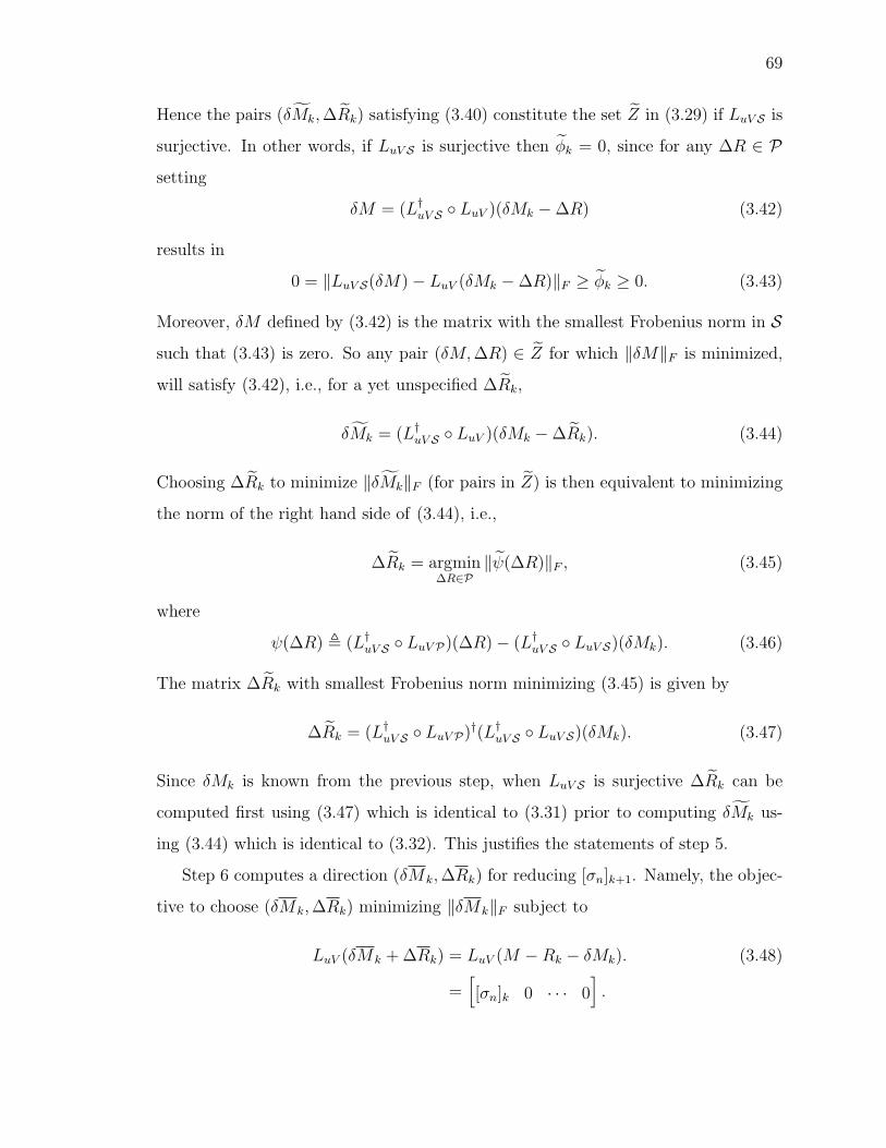
69

Hence the pairs (δMk,ΔRk) satisfying (3.40) constitute the set Z in (3.29) if LuV S is

surjective. In other words, if LuV S is surjective then φk = 0, since for any ΔR ∈ Psetting

δM = (L†uV S ◦ LuV )(δMk −ΔR) (3.42)

results in

0 = ‖LuV S(δM)− LuV (δMk −ΔR)‖F ≥ φk ≥ 0. (3.43)

Moreover, δM defined by (3.42) is the matrix with the smallest Frobenius norm in Ssuch that (3.43) is zero. So any pair (δM,ΔR) ∈ Z for which ‖δM‖F is minimized,

will satisfy (3.42), i.e., for a yet unspecified ΔRk,

δMk = (L†uV S ◦ LuV )(δMk −ΔRk). (3.44)

Choosing ΔRk to minimize ‖δMk‖F (for pairs in Z) is then equivalent to minimizing

the norm of the right hand side of (3.44), i.e.,

ΔRk = argminΔR∈P

‖ψ(ΔR)‖F , (3.45)

where

ψ(ΔR) � (L†uV S ◦ LuV P)(ΔR)− (L†

uV S ◦ LuV S)(δMk). (3.46)

The matrix ΔRk with smallest Frobenius norm minimizing (3.45) is given by

ΔRk = (L†uV S ◦ LuV P)

†(L†uV S ◦ LuV S)(δMk). (3.47)

Since δMk is known from the previous step, when LuV S is surjective ΔRk can be

computed first using (3.47) which is identical to (3.31) prior to computing δMk us-

ing (3.44) which is identical to (3.32). This justifies the statements of step 5.

Step 6 computes a direction (δMk,ΔRk) for reducing [σn]k+1. Namely, the objec-

tive to choose (δMk,ΔRk) minimizing ‖δMk‖F subject to

LuV (δMk +ΔRk) = LuV (M −Rk − δMk). (3.48)

=[[σn]k 0 · · · 0

].

70

As in step 5, the linear operator LuV approximates the smallest singular value function

σn(·). Hence (3.48) is an approximation of the constraint σn(M −Rk −ΔRk − δMk −δMk) = 0. Using the same arguments used above for step 5, pairs (δMk,ΔRk)

satisfying (3.48) are in Z if LuV S is surjective. In other words, if LuV S is surjective,

then φk = 0 and the pair (δMk,ΔRk) ∈ Z minimizing ‖δMk‖F satisfies

δMk = (L†uV S ◦ LuV )(M −Rk −ΔRk − δMk), (3.49)

where ΔRk is chosen to be the smallest norm matrix in P minimizing the norm of

the right side of (3.49), i.e.,

ΔRk = argminΔR∈P

‖ψ(ΔR)‖F , (3.50)

where

ψ(ΔR) = (L†uV S ◦ LuV P)(ΔR)

− (L†uV S ◦ LuV )(M −Rk − δMk).

(3.51)

The matrix ΔRk with smallest Frobenius norm minimizing (3.50) is given by

ΔRk = (L†uV S ◦ LuV P)

†(L†uV S ◦ LuV )(M −Rk − δMk). (3.52)

This completes the justification of step 6.

What remains is to specify the step size αk. To choose αk, we would like to

minimize the Lyapunov function Pk+1 = [σn]k+1 + gk+1‖δMk+1‖F in the direction of

ΔRk and δMk in step 7. Due to differentiability issues of the singular value function

σn(·), we will instead minimize a quadratic function f(k)ub (α) in (3.37) which upper

bounds (verified in the proof of Theorem 3.10) the decrease in the Lyapunov function,

i.e., Pk+1(α) − Pk ≤ f(k)ub (α). We will show that choosing αk to be the minimum

of this upper bound f(k)ub will imply that the sequence of Lyapunov functions {Pk}

converges. Unlike the usual definition of Lyapunov energy functions, we will not

guarantee that {Pk} converges to zero, but rather a positive constant, {Pk} → d =

g∗‖δM∗‖F . This will be sufficient for guaranteeing the necessary conditions are met

at the terminating values for δM∗ and R∗ if Assumption 3.1 and two additional

assumptions to be described in Section 3.5. The next subsection addresses details for

the implementation of Algorithm 1 in software.

71

3.4.1 Algorithm 1 Implementation

Implementing a few steps of Algorithm 1 require some explanation. To implement

steps 5 and 6 of Algorithm 1, the pseudoinverse LuV S is computed via Kronecker

products and the vec operator [41,42]. Applying the vec operator to LuV S we obtain

vec(LuV S(δM)) = (V � ⊗ uH) vec(δM)

= (V � ⊗ uH)BSζ,

where ζ respresents δM in the orthonormal basis {S1, · · · , Sk} and

BS � [vec(S1), · · · , vec(Sk)].

Taking the real and imaginary components of vec(LuV S(δM)) we obtain⎡⎣(Re[LuV S(δM)])�

(Im[LuV S(δM)])�

⎤⎦ =

⎡⎣Re[(V � ⊗ uH)BS ]

Im[(V � ⊗ uH)BS ]

⎤⎦ ζ.Let NS ∈ C

2(m−n+1)×k and NP ∈ C2(m−n+1)×r be given by

NS =

⎡⎣Re[(V �k ⊗ [un]

Hk )BS ]

Im[(V �k ⊗ [un]

Hk )BS ]

⎤⎦ ,NP =

⎡⎣Re[(V �k ⊗ [un]

Hk )BP ]

Im[(V �k ⊗ [un]

Hk )BP ]

⎤⎦ ,where BP � [vec(P1), · · · , vec(Pr)]. With this notation, ΔRk of (3.31) and δMk

of (3.32) satisfy

vec(ΔRk) = BP(N†SNP)

†N †SNSζk

vec(δMk) = BSN†S

⎡⎣Re[(V �k ⊗ [un]

Hk ) vec(δMk −ΔRk)]

Im[(V �k ⊗ [un]

Hk ) vec(δMk −ΔRk)]

⎤⎦,

72

where ζk represents δMk in {S1, · · · , Sk}. Similarly, ΔRk in (3.35) and δMk in (3.36)

satisfy

vec(ΔRk) = BP(N†SNP)

†N †S∗⎡⎣Re[(V �

k ⊗ [un]Hk ) vec(M −Rk − δMk)]

Im[(V �k ⊗ [un]

Hk ) vec(M −Rk − δMk)]

⎤⎦vec(δMk) = BSN

†S∗⎡⎣Re[(V �

k ⊗ [un]Hk ) vec(M −Rk −ΔRk − δMk)]

Im[(V �k ⊗ [un]

Hk ) vec(M −Rk −ΔRk − δMk)]

⎤⎦Now we consider step 9 that requires the minimization of the function f

(k)ub in (3.37)

with respect to the step size αk. One such method for this minimization is a one

dimensional constrained line search for αk ∈ [0, 1]. Since a decrease in the Lyapunov

energy function Pk+1 is guaranteed for α sufficiently small, an appropriate initial guess

for αk is 0. Alternatively, one can analytically solve for the minimizer since f(k)ub is a

quadratic function of α. Namely

f(k)ub (α) = α(c

(k)1 + c

(k)2 α),

where c(k)1 and c

(k)2 are given by

c(k)1 = −

([σn]k2

+ 2Re[〈δMk, δMk − δMk〉])

c(k)2 = ak + ‖δMk − δMk‖2F .

The minimizer of f(k)ub in the interval [0, 1] is given by

αk = min

{c(k)1

2c(k)2

, 1

},

if c(k)2 = 0 and 0 otherwise. Either a line search or the analytical solution to minimizing

f(k)ub over the interval [0, 1] can be used for step 9.

73

3.5 Convergence of Algorithm 1

Convergence of the P–robustness problem requires a structural condition on the

property space P :

Assumption 3.2. Each nonzero property matrix R ∈ P is full rank, i.e., rankR = n.

If there exists a nonzero R ∈ P which is not full rank, σn(M − δM − ηR) may be

finite (and possibly optimal) as η → ∞. Convergence to a finite property matrix is

guaranteed to exist if for all nonzero R ∈ P , rank(R) = n, i.e., R is full row rank;

hence, the infimum in (3.4) and (3.6) can be replaced with the minimum since the

associated optimal property matrix is bounded.

Two additional assumptions aid in proving convergence of Algorithm 1.

Assumption 3.3. The sequence {gk} computed by Algorithm 1 is bounded away from

zero.

Assumption 3.4. The sequence {[σn−1]k} computed by Algorithm 1 is bounded away

from zero.

The sequence {gk} in Assumption 3.3 essentially measures the surjectivity of LuV S .

When {gk} is bounded away from zero, the algorithm converges to a minimizer at

which LuV S is surjective. Assumption 3.4 requires that the (n − 1)th singular value,

[σn−1]k, is nonzero. In addition, we will assume that LuV S is surjective for each unit

vector u ∈ Cn and each matrix V ∈ C

m×(m−n+1) with columns which are orthogonal

unit vectors which can appear as singular vectors of M − δMk − Rk as introduced

in Assumption 3.1. Note, this set of u and V satisfy uHu = u†u = 1 and V HV =

V †V = I. To prove convergence of Algorithm 1, we need to establish a few necessary

lemmas. The first lemma bounds [σn]k+1(α) as a function of α.

Lemma 3.7. Let u and V contain lsv and rsv of M − δMk − Rk, respectively, as in

Algorithm 1. If LuV S is surjective, then for all α ∈ (0, 1),

σn

(M − δMk −Rk − α(δMk − δMk +ΔRk)

)

74

is bounded from above by

(1− α)[σn]k + α2ak (3.53)

where [σn]k � σn(M − δMk −Rk) and ak is given in (3.38).

Proof. See appendix.

The next lemma constructs an upper bound on the norm ‖δMk+1‖F as a function of

α. To state the upper bound, we require the following linear orthogonal projection

operators from the proofs of Lemmas 3.4 and 3.5:

Q1 � (L†uV S ◦ LuV S) (3.54)

Q2 � I − (L†uV S ◦ LuV P)(L

†uV S ◦ LuV P)

†. (3.55)

Lemma 3.8. Let u and V contain lsv and rsv of M − δMk − Rk, respectively, as in

Algorithm 1. If LuV S is surjective, then for all α ∈ [0, 1]

‖(1− α)δMk + αδMk‖F ≤ ‖δMk‖F + α‖δMk‖F

+ bk(‖(1− α)δMk + α(Q2 ◦Q1)(δMk)‖2F − ‖δMk‖2F

),

(3.56)

where bk and δMk are given in Algorithm 1 and Q1 and Q2 are given in (3.54)

and (3.55), respectively.

Proof. See appendix.

Proving convergence of Algorithm 1 will be achieved by appealing to a Lyapunov

function Pk = [σn]k + gk‖δMk‖F . Given Assumptions 3.2 and 3.3, we will show i)

Pk+1 − Pk ≤ f(k)ub (αk) ≤ 0 and ii) that f

(k)ub (αk) < 0 if the necessary conditions of

δMk and δRk in Theorem 3.2 are not satisfied. Since Pk is nonnegative for each k,

proving that {Pk} is nonincreasing implies it is a bounded monotone function so the

sequence converges, i.e., Pk+1 − Pk → 0. Hence this will prove that f(k)ub (αk) → 0

which implies convergence to a pair δM∗ and R∗ satisfying the necessary conditions

in Theorem 3.2. The next lemma is the key step in relating f(k)ub and the necessary

conditions in Theorem 3.2.

75

Lemma 3.9. Let R ∈ P and δM ∈ S satisfy rank[M−R−δM ] < n, i.e., a candidate

solution. R and δM satisfy the necessary conditions in Theorem 3.2 if and only if

(Q2 ◦Q1)(δM) = δM,

where Q1 and Q2 are given in (3.54) and (3.55), respectively, with u the nth lsv of

M −R− δM and V has columns containing the nth through mth rsv of M −R− δM .

Proof. See appendix.

The next Theorem proves that if Algorithm 1 is carried out to infinite precision,

then the algorithm converges to a necessary condition for an optimal solution R∗

and δM∗. The stopping conditions in Algorithm 1 guarantee that the algorithm

terminates. The parameter ε determines how far the terminal points δMk and Rk are

from satisfying the necessary conditions.

Theorem 3.10. If Assumptions 3.2-3.4 hold, then the sequence {Pk} computed by

Algorithm 1 converges, where

Pk � [σn]k + gk‖δMk‖F . (3.57)

Further, the sequences {δMk} and {Rk} have limit points δM∗ and R∗ satisfying the

necessary conditions of Theorem 3.2.

Proof. First we show that Pk+1 − Pk ≤ f(k)ub (αk). Because gk is nonincreasing,

Lemma 3.7 and 3.8 imply that

Pk+1 − Pk

= [σn]k+1 + gk+1‖δMk+1‖F − ([σn]k + gk‖δMk‖F )

≤ −αk[σn]k + akα2k + αkgk‖δMk‖F − gkbk‖δMk‖2F

+ gkbk‖(1− αk)δMk + αk(Q2 ◦Q1)(δMk)‖2F

76

Since gk ≤ [σn]k/(2‖δMk‖F ),

Pk+1 − Pk

≤ −[σn]k2

αk + akα2k − gkbk‖δMk‖2F

+ gkbk‖(1− αk)δMk + αk(Q2 ◦Q1)(δMk)‖2F� f

(k)ub (αk).

Note that f(k)ub (α) is a quadratic function of α and f

(k)ub (0) = 0. So there exists

constants c(k)1 and c

(k)2 such that

f(k)ub (α) = c

(k)1 α + c

(k)2 α2.

Careful inspection of f(k)ub (α) shows that c

(k)2 ≥ 0, i.e., f

(k)ub (α) admits a global min-

imum. Since gk, bk, and [σn]k are all nonnegative, c(k)1 ≤ 0 if the coefficient of the

linear term in the quadratic

‖(1− αk)δMk + αk(Q2 ◦Q1)(δMk)‖2F − ‖δMk‖2F

is nonpositive. This is clearly the case since ‖(Q2 ◦Q1)(δMk)‖F ≤ ‖δMk‖F . Further,c(k)1 = 0 if and only if [σn]k = 0 and (Q2 ◦Q1)(δMk) = δMk since gk > 0 by Assump-

tion 3.3. Equivalently, Lemma 3.9 implies that c(k)1 = 0 if and only if the necessary

conditions are satisfied. Since αk is chosen to minimize f(k)ub over the interval [0, 1],

f(k)ub (αk) < 0 so long as the necessary conditions are not satisfied.

Thus {Pk} is nonnegative and decreasing since Pk+1 − Pk ≤ f(k)ub (αk) ≤ 0. By the

monotone convergence theorem, {Pk} converges, i.e., Pk+1 − Pk → 0. To prove that

we converge to a necessary condition, we will prove that the sequence {c(k)1 } converges

to zero. Based on Lemma 3.9, this implies that a necessary condition is satisfied.

Since Pk+1 −Pk ≤ f(k)ub (αk) ≤ 0 and Pk+1 −Pk → 0, the sequence {f (k)

ub (αk)} → 0.

As long as {c(k)2 } is bounded, this implies that {c(k)1 } → 0 as desired. The sequence

{c(k)2 } is unbounded only if the quadratic coefficient of the function

akα2k − gkbk‖δMk‖2F+ gkbk‖(1− αk)δMk + αk(Q2 ◦Q1)(δMk)‖2F

(3.58)

77

goes unbounded. The quadratic term coefficient in (3.58) is given by ak + gkbk‖(I −Q2 ◦Q1)δMk‖2 and by construction bk‖(I −Q2 ◦Q1)δMk‖2F ≤ bk‖δMk‖2F ≤ ‖δMk‖F .Since {Pk} converges and {gk} > 0, ‖δMk‖F is bounded. By (3.38), ak ≤ ‖δMk −δMk − ΔRk‖2F/[σn−1]k, which by Assumption 3.4 is bounded if ΔRk is bounded, or

equivalently if Rk is bounded.

Assume for contradiction that {Rk} is unbounded. Since {Pk} converges, [σn]k

is bounded. Since {gk} > 0, {δMk} is bounded as well. Let Rmin be the norm one

property matrix minimizing σn, i.e., Rmin = argminR∈P,‖R‖F=1 σn(R). By Assump-

tion 3.2, σn(Rmin) > 0 and for any R ∈ P , σn(R) ≥ ‖R‖Fσn(Rmin). Hence, letting

uk be the nth lsv of M −Rk − δMk, for sufficiently large k

[σn]k = ‖uHk (M −Rk − δMk)‖2

≥ ‖uHk Rk‖2 − ‖uHk (M − δMk)‖2

≥ σn(Rk)− ‖uHk (M − δMk)‖2

≥ ‖Rk‖Fσn(Rmin)− ‖uHk (M − δMk)‖2.

Hence, if ‖Rk‖F → ∞, then [σn]k → ∞ contradicting that {Pk} converges. Hence

{ΔRk} is bounded and thus {ak} and {c(k)2 } are bounded. This implies that as

k → ∞, (Q2 ◦ Q1)(δMk) → δMk, i.e., the two necessary conditions in Theorem 3.2

are satisfied as k → ∞. Finally, since {gk} > 0 and {Pk} converges, the sequence of

perturbations {δMk} has a bounded accumulation point δM∗. Since δM∗ satisfies the

two necessary conditions, the sequence {ΔRk} has an accumulation point ΔR∗ = 0,

i.e., Rk → R∗, completing the proof.

78

3.6 Numerical Examples

3.6.1 Example 1

Consider the third example in [25] (also appears in [32] and [29]), which in the

P–robustness framework has system matrix M , structured perturbations δM , and

property matrices R given by

M =[A B

]δM =

[δA δB

]∈ R

3×4

R = λ[I 0

]∈ C

3×4,

where

A =

⎡⎢⎢⎢⎣1 1 1

0.1 3 5

0 −1 −1

⎤⎥⎥⎥⎦ , B =

⎡⎢⎢⎢⎣1

0.1

0

⎤⎥⎥⎥⎦ .With initial guesses δM0 = 0 and R0 = [jI, 0], and ε = 10−10, Algorithm 1 terminates

in 9 iterations. The P–robustness of M with respect to parameter variations in S is

computed to be r(M ;S,P) = 0.057737. The minimizing property and perturbation

matrices are R∗ = (0.9824 + 0.9731j)[I, 0] and δM∗ = [δA∗, δB∗], respectively, where

δA∗ = 10−4

⎡⎢⎢⎢⎣−5.8878 −0.49659 0.29287

168.48 14.210 −8.3803

167.31 14.111 −8.3221

⎤⎥⎥⎥⎦δB�

∗ = 10−3[1.1427 15.754 49.685

].

Upon termination, σn(M − δM∗ −R∗) = 2.8944× 10−16 which is approximately zero.

These results are consistent with [25] and [29]. As noted in [29], we cannot compare

the results of this example to [32] due to the different norm used therein (largest

singular value of δM versus the Frobenius norm).

79

3.6.2 Example 2

Consider the example in [30], which in the P–robustness framework has a fixed

system matrix M , structured perturbations δM , and property matrices R are given

by

M =

⎡⎣A�0 0 C�

0

0 A�1 C�

1

⎤⎦δM =

⎡⎣δA�0 0 δC�

0

0 δA�1 δC�

1

⎤⎦ ∈ R4×5

R = λ[I 0

]∈ C

4×5,

where

A0 =

⎡⎣−1 2

0 −2

⎤⎦,A1 =

⎡⎣−3 0.1

5 −1

⎤⎦C0 =

[1 0

], C1 =

[1 1

].

The perturbation space S is real and does not allow perturbations of the off-diagonal

entries of M . In [30], the distance to the nearest SMS SLTI system is computed to

satisfy

0.0506 ≤ r(M ;S,P) ≤ 0.4570.

Setting the terminating condition for ε = 10−15 and initial guesses δM0 = 0 and

R0 = 0, the Algorithm 1 terminated in 13 iterations. The distance r(M ;S,P) is

computed to be r(M ;S,P) = 0.071821 where R∗ = −0.9065[I 0

],

δM∗ = 10−3

⎡⎢⎢⎢⎢⎢⎢⎣−21.5 −39.3 0 0 0

−0.8 −1.4 0 0 0

0 0 1.2 0.5 0

0 0 51.8 21.7 0

⎤⎥⎥⎥⎥⎥⎥⎦ , (3.59)

and σn(M − δM∗ −R∗) = 5.256× 10−16 ≈ 0. Note that φR(Σ) = 0.071821 is between

0.0506 and 0.4570.

80

3.7 Conclusion

In this work, the P–robustness framework developed in [38] is used to solve a fam-

ily of robustness problems. Specifically, the Frobenius norm metric is used to measure

the P–robustness of M with respect to perturbations in S. Necessary conditions for

a minimal rank reducing perturbation are proven in Theorem 3.2. The necessary

conditions motivate Algorithm 1 for computing both the metric r(M S,P) and the

minimizing property matrix R∗ and perturbation matrix δM∗.

In future work, we will modify Algorithm 1 to solve P–robustness problems with

singular property matrices, i.e., rank(R) < n. This modification will address the case

where the norm of the optimal property matrix R∗ is unbounded. In addition, we

expect that Algorithm 1 can be modified to compute the P–robustness of M using

the spectral norm metric, i.e., minimizing σ1(δM∗). Although the Frobenius norm

may be a more accurate measure of robustness, extending to the spectral norm metric

unifies the robustness property literature.

3.8 Chapter 3 Appendix

3.8.1 Surjectivity

This section explores conditions for surjectivity of maps LuV and LuV S . The first

result is that LuV : Cn×m → C1×(m−n+1) is surjective if u is a unit vector and V has

mutually orthonormal columns.

Proposition 3.11. If u ∈ Cm is a unit vector and V ∈ C

m×(m−n+1) V has mutually

orthonormal columns then LuV : Cn×m → C1×(m−n+1) is surjective.

Proof. Represent the map LuV as the (V �⊗uH) which maps vec(M) into Cm−n+1. As

such, rank(V �⊗uH) = rank(V )∗rank(u) = m−n+1 (see [43, Corollary 13.11] for the

rank of Kronecker product). Since the matrix representing LuV has rank m− n+ 1,

the range LuV (Cn×m) has dimension m−n+1 (with respect to complex coefficients),

i.e., LuV (Cn×m) = C

1×(m−n+1).

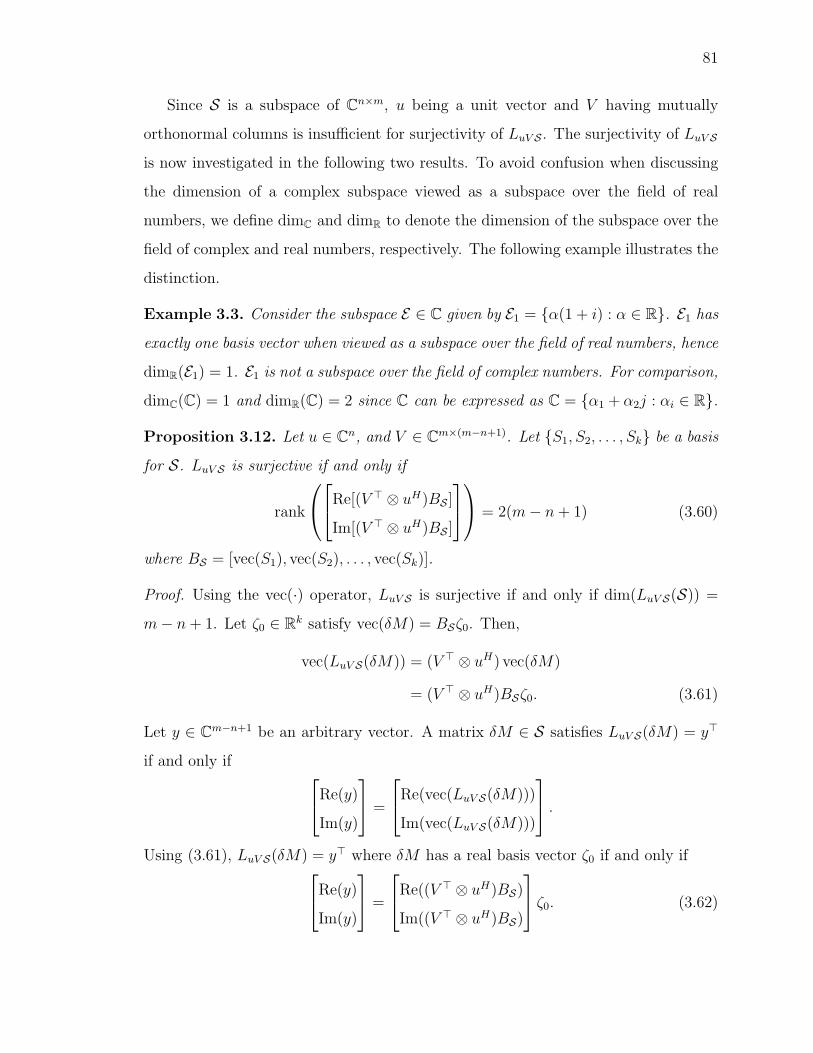
81

Since S is a subspace of Cn×m, u being a unit vector and V having mutually

orthonormal columns is insufficient for surjectivity of LuV S . The surjectivity of LuV S

is now investigated in the following two results. To avoid confusion when discussing

the dimension of a complex subspace viewed as a subspace over the field of real

numbers, we define dimC and dimR to denote the dimension of the subspace over the

field of complex and real numbers, respectively. The following example illustrates the

distinction.

Example 3.3. Consider the subspace E ∈ C given by E1 = {α(1 + i) : α ∈ R}. E1 hasexactly one basis vector when viewed as a subspace over the field of real numbers, hence

dimR(E1) = 1. E1 is not a subspace over the field of complex numbers. For comparison,

dimC(C) = 1 and dimR(C) = 2 since C can be expressed as C = {α1 + α2j : αi ∈ R}.

Proposition 3.12. Let u ∈ Cn, and V ∈ C

m×(m−n+1). Let {S1, S2, . . . , Sk} be a basis

for S. LuV S is surjective if and only if

rank

⎛⎝⎡⎣Re[(V � ⊗ uH)BS ]

Im[(V � ⊗ uH)BS ]

⎤⎦⎞⎠ = 2(m− n+ 1) (3.60)

where BS = [vec(S1), vec(S2), . . . , vec(Sk)].

Proof. Using the vec(·) operator, LuV S is surjective if and only if dim(LuV S(S)) =

m− n+ 1. Let ζ0 ∈ Rk satisfy vec(δM) = BSζ0. Then,

vec(LuV S(δM)) = (V � ⊗ uH) vec(δM)

= (V � ⊗ uH)BSζ0. (3.61)

Let y ∈ Cm−n+1 be an arbitrary vector. A matrix δM ∈ S satisfies LuV S(δM) = y�

if and only if ⎡⎣Re(y)Im(y)

⎤⎦ =

⎡⎣Re(vec(LuV S(δM)))

Im(vec(LuV S(δM)))

⎤⎦ .Using (3.61), LuV S(δM) = y� where δM has a real basis vector ζ0 if and only if⎡⎣Re(y)

Im(y)

⎤⎦ =

⎡⎣Re((V � ⊗ uH)BS)

Im((V � ⊗ uH)BS)

⎤⎦ ζ0. (3.62)

82

LuV S is surjective if and only if for each y ∈ Cm−n+1, there exists ζ0 ∈ R

k such

that (3.62) holds. Hence, LuV S is surjective if and only if⎡⎣Re((V � ⊗ uH)BS)

Im((V � ⊗ uH)BS)

⎤⎦is full row rank, i.e., (3.60) is satisfied.

Corollary 3.13. Let u ∈ Cn, and V ∈ C

m×(m−n+1). Then LuV S is surjective only if

dimR S ≥ 2(m− n+ 1).

Proposition 3.12 requires at least 2(m − n + 1) columns of the basis matrix BS

to lie outside of the null space of (V � ⊗ uH). It is both the dimension of S (i.e.,

the number of columns of BS) and the null space of (V � ⊗ uH) that determines

surjectivity of LuV S . Not all pairs of matrices u ∈ Cn and V ∈ C

m×(m−n+1) induce a

linear operator LuV S which is surjective. For example, if u = 0 or V = 0 clearly LuV S

is not surjective.

We complete this discussion on surjectivity of the linear operators LuV S by con-

sidering the special case of real perturbations, i.e., S ⊂ Rn×m. In this subset of

P–robustness problems, the added structure leads to several strongly sufficient condi-

tions for surjectivity that have analogous results for the particular problem considered

in [28].

Corollary 3.14. Let S = Rn×m and rank(Im(M − R)) = n for a fixed R ∈ P. Let

δM ∈ S be any perturbation such that rank[M −R− δM ] < n and let u ∈ Cn be the

nth lsv of M −R− δM and V ∈ Cm×(m−n+1) have columns equal to the last m−n+1

rsv of M −R− δM . Then LuV S is surjective.

Proof. Since S = Rn×m, without loss of generality let BS = Imn. Let y1, y2 ∈ C

m−n+1

be any vectors such that y�1 Re[V � ⊗ uH ] + y�2 Im[V � ⊗ uH ] = 0. Using appropriate

Kronecker product identities, one can verify (V � ⊗ uH) = V �(Im ⊗ uH). Recall that

83

(A + B) ⊗ (C +D) = A ⊗ C + B ⊗ C + A ⊗D + B ⊗D for matrices A,B,C,D of

appropriate dimension. Hence, applying BS = Imn, we observe⎡⎣Re[(V � ⊗ uH)BS ]

Im[(V � ⊗ uH)BS ]

⎤⎦=

⎡⎣Re(V �) −Im(V �)

Im(V �) Re(V �)

⎤⎦⎡⎣Im ⊗ Re(uH)

Im ⊗ Im(uH)

⎤⎦� V

�

⎡⎣Im ⊗ Re(uH)

Im ⊗ Im(uH)

⎤⎦ .Since V has orthonormal columns,

V HV = Re(V �) Re(V )− Im(V �) Im(V ) + j(Re(V �) Im(V ) + Im(V �) Re(V ))

= Im−n+1

implying

V�

⎡⎣Re(V ) −Im(V )

Im(V ) Re(V )

⎤⎦ = I2(m−n+1).

Thus V�has a right inverse and must have full row rank. Consequently, [y�1 , y

�2 ]V

�=

0 only if y1 = y2 = 0. Let [ν�1 , ν�2 ] = [y�1 , y

�2 ]V

�. Then ν�1 (Im ⊗ Re(uH)) + ν2(Im ⊗

Im(uH)) = 0. However, this implies

[ν1 ν2

]⎡⎣Re(uH)Im(uH)

⎤⎦ = 0. (3.63)

By [28, Proposition 3.3], since rank(Im(M − R)) = n and S = Rn×m any left null

vector u of M − R − δM satisfies rank[Re(u), Im(u)] = 2 which by (3.63) implies

ν1 = ν2 = 0 and thus y1 = y2 = 0, i.e., (3.60) is full row rank. Hence LuV S is

surjective by Proposition 3.12.

Corollary 3.14 provides conditions sufficient for surjectivity. The next two results

use a structural condition which is stronger than surjectivity of LuV S . Proposition 3.15

proves that for any unit vector u and real perturbation space S satisfying (3.64) a

perturbation matrix δM ∈ S exists such that u is a left null vector of M − δM .

84

Proposition 3.15. Let u ∈ Cn be unit vector and m ≥ n ≥ 2. Let S ⊂ R

n×m be a real

vector space having basis {S1, S2, . . . , Sk} and let BS = [vec(S1), vec(S2), . . . , vec(Sk)].

If

rank[Z(u)] � rank

⎛⎝⎡⎣Im ⊗ Re(uH)

Im ⊗ Im(uH)

⎤⎦BS

⎞⎠ = 2m, (3.64)

then for each M ∈ Cn×m, there exists a perturbation δM ∈ S such that u is a left

null vector of M − δM , i.e., uH(M − δM) = 0.

Proof. Let M ∈ Cn×m. Let xH0 � −uHM . If x0 = 0, then δM = 0 satisfies the

required conditions trivially. Assume x0 = 0. Since Z(u) is full row rank, Z†(u) is a

right inverse of Z(u). Let δM ∈ S be the matrix satisfying vec(δM) = BSζ where

ζ ∈ Rk satisfies

ζ = Z†(u)

⎡⎣Re(cj(x))Im(cj(x))

⎤⎦ ,where cj(x) = Re(x) − j Im(x) is the complex conjugate. Then since vec(uHδM) =

(uHδM)� = (Im ⊗ uH) vec(δM) and vec(δM) = BSζ,⎡⎣Re((uHδM)�)

Im((uHδM)�)

⎤⎦ = Z(u)ζ =

⎡⎣Re(cj(x))Im(cj(x))

⎤⎦ .Hence uH(M − δM) = −xH0 +xH0 = 0 implying u is a left null vector of M − δM .

Proposition 3.16 proves that the condition in (3.64) guarantees that if rank[M −δM − R] = n − 1 then there exists a neighborhood of M − δM − R for which rank

reducing perturbations exist with a Frobenius norm bounded by the growth of the

nth singular value in this neighborhood. A similar unproven result is proposed in [38].

Proposition 3.16. Let δM ′ ∈ S and R′ ∈ P be such that M �M−δM ′−R′ ∈ Cn×m

satisfies rank[M ] = n−1 and let u be the nth lsv of M . Let S ⊂ Rn×m be a real vector

space with orthonormal basis {S1, S2, . . . , Sk} with

BS = [vec(S1), vec(S2), . . . , vec(Sk)].

85

By orthonormal we mean 〈Si, Sj〉 = δij, where δij = 1 if i = j and 0 otherwise. If

rank[Z(u)] � rank

⎛⎝⎡⎣Im ⊗ Re(uH)

Im ⊗ Im(uH)

⎤⎦BS

⎞⎠ = 2m, (3.65)

there exists constants c and K such that for every N ∈ Cn×m with ‖N‖F < c there is

a δM ∈ S satisfying ‖δM‖F ≤ Kσn(M −N) and rank(M −N − δM) < n.

Proof. Since the last singular value of M is distinct there exists a neighborhood of M

(call it M−N for ‖N‖F < d) wherein all matrix valued functions N(α) which depend

analytically on the real scalar α and satisfy ‖N(·)‖F < d have a nth lsv function u(α)

of M − N(α) which can be chosen to be an analytic function of α, (See [39, 44] for

more details). As a result, there exists c > 0 small enough for which there exists

ε = ε(c) > 0 such that for each N with ‖N‖F < c the nth lsv u of M −N satisfies

σ2m(Z(u)) ≥ ε > 0. (3.66)

Consider one specific N satisfying ‖N‖F < c and nth lsv u of M − N . Let x0 ∈ Cm

be the unique vector satisfying

uH(M −N)− xH0 = 0.

We will now construct a perturbation δM ∈ S such that uHδM = xH0 . If x0 = 0, then

rank(M − N) < n and δM = 0 satisfies the conditions of the lemma. If x0 = 0, we

note that uHδM = xH0 if and only if Re(xH0 ) = Re(uHδM) and Im(xH0 ) = Im(uHδM).

Equivalently, uHδM = xH0 if and only if⎡⎣vec(Re(xH0 ))vec(Im(xH0 ))

⎤⎦ =

⎡⎣Re(vec(uHδM))

Im(vec(uHδM))

⎤⎦ . (3.67)

Since vec(uHδM) = (Im ⊗ uH) vec(δM) and vec(δM) = BSζ0 for some ζ0 ∈ Rk,

uHδM = xH0 if and only if ⎡⎣vec(Re(xH0 ))vec(Im(xH0 ))

⎤⎦ = Z(u)ζ0.

86

Since Z(u) has full row rank by (3.66), Z(u)† is a right inverse. Then δM � BSζ0

with

ζ0 � Z(u)†

⎡⎣vec(Re(xH0 ))vec(Im(xH0 ))

⎤⎦satisfies uHδM = xH0 . Thus uH(M − N − δM) = 0, i.e., rank(M − N − δM) < n.

What remains is the show that is the bound on ‖δM‖F . Since BS has orthonormal

columns ‖δM‖F = ‖ζ0‖2. Hence

‖δM‖F ≤ σ1(Z(u)†)

∥∥∥∥∥∥⎡⎣vec(Re(xH0 ))vec(Im(xH0 ))

⎤⎦∥∥∥∥∥∥2

=1

ε‖uH(M −N)‖2.

Since u is the nth lsv of M −N , ‖uH(M −N)‖2 = σn(M −N). Letting K = 1/ε, we

obtain the desired bound ‖δM‖ ≤ Kσn(M −N).

Propositions 3.12, 3.15, and 3.16 demonstrate the usefulness of fixing a basis for

S (and later for P) for verifying system properties.

3.8.2 Additional Proofs

Proof of Lemma 3.3.

Step 1: First we show that every analytic path ga : [0, 1] → W from W1 to W2

has an analytic unsigned nth singular value function fa : [0, 1] → R such that fa(s) =

H(ga(s)), i.e., H is an unsigned nth singular value function for each analytic path inW .

Without loss of generality assume fa(0) = H(ga(0)). Recall H was constructed to be

consistent with fg, the unsigned nth singular value function associated with the curve

g. Construct a continuous closed path by connecting ga(0) with g(0) in W1 and ga(1)

with g(1) in W2. Since σn is continuous and nonzero in W1 ∪W2, σn is continuous on

the closed path and thus sign(fa(1)) = sign(fg(1)), i.e., fa(s) = H(ga(s)) as desired.

Consequently, H can be used for an unsigned nth singular value for any analytic curve

in W .

87

Step 2: if (ζ , ρ) ∈ W1 ∪ W2 then the nth singular value of M(ζ , ρ) is distinct

and hence the nth lsv and rsv are unique up to multiplication by unitary scalars.

By [39, Theorem 3], there exists a neighborhood W0 ⊂ W1∪W2 of (ζ , ρ) and analytic

(unsigned) singular vector functions u : W0 → Cn and v : W0 → C

m such that for all

(ζ, ρ) ∈ W0,

uH(ζ, ρ)M(ζ, ρ)v(ζ, ρ) = H(ζ, ρ).

Since u, v, and M(ζ, ρ) are analytic, so is H.

To take the derivative ∂ ˜H(˜ζ,ρ)∂ζi

, we consider replacing ζ with a complex argument

z.3 The complex partial derivative with respect to zi at z = ζ is

∂H(z, ρ)

∂zi=∂uH

∂ziM(ζ , ρ)v + uH

∂M(z, ρ)

∂ziv

+ uHM(ζ , ρ)∂v

∂zi

= H(ζ , ρ)

(∂uH

∂ziu+ vH

∂v

∂zi

)− uHSiv,

since u and v are singular value functions, i.e.,

M(ζ , ρ)v(ζ , ρ) = H(ζ , ρ)u(ζ , ρ)

and

uH(ζ , ρ)M(ζ , ρ) = H(ζ , ρ)vH(ζ , ρ).

However, since 1 = uH u, we obtain 0 = ∂uH

∂ziu +

(∂uH

∂ziu)H

. Hence Re(

∂uH

∂ziu)= 0.

Similarly, Re(vH ∂v

∂zi

)= 0. The real derivative of H with respect to ζi is given by

∂H(ζ , ρ)

∂ζi= Re

[∂H(z, ρ)

∂zi

]= −Re(uH(ζ , ρ)Siv(ζ , ρ)).

The same argument holds for computing ∂ ˜H(˜ζ,ρ)∂ρi

= −Re(uH(ζ , ρ)Piv(ζ , ρ)).

3 Rigorously, we should define a new function with a complex domain, but we have chosen to keepthe presentation more direct.

88

Step 3: what remains is to show that H is Frechet differentiable for (ζ0, ρ0) ∈W \W1 ∪W2, i.e., points where M(ζ0, ρ0) drops rank. Although σn(M(ζ0, ρ0)) = 0,

the nth lsv is unique (up to unitary scalar multiplication) since the last singular

value is distinct and M(ζ0, ρ0) has fewer rows than columns. The problem with the

nth (unsigned) rsv is that it is not unique since M(ζ, ρ0) has a right null space of

dimension m− n+ 1. However, not all nth (unsigned) rsv can be part of an analytic

singular value function for analytic paths passing through (ζ0, ρ0). Let gb : [0, 1] → W

be an analytic curve from W1 to W2 with gb(0.5) = (ζ0, ρ0). By [39], there exists

analytic nth (unsigned) lsv and rsv functions ub : [0, 1] → Cn and vb : [0, 1] → C

m,

respectively, associated with the unsigned nth singular value function H(gb(·)). Sincefor each s = 0.5, M(gb(s)) is a fixed matrix with a nonzero nth singular value, the

product ub(s)vHb (s) is unique (even though ub(s) and vb(s) are not unique). The same

uniqueness result holds for analytic curves from W2 to W1 passing through (ζ0, ρ0).

For analytic paths in W \W1 ∪W2 passing through (ζ0, ρ0), the right null space of

M(ζ, ρ) changes analytically and hence one can choose ub(0.5) and vb(0.5) as the nth

unsigned lsv and rsv along these paths as well. Because W , W1, and W2 are simply

connected, there exists a neighborhood W0 of (ζ0, ρ0) and analytic singular vector

functions u0 : W0 → Cn and v0 : W0 → C

m such that

uH0 (ζ, ρ)M(ζ, ρ)v0(ζ, ρ) = H(ζ, ρ)

for all (ζ, ρ) ∈ W0. Using the same arguments as in Step 2 it follows that H is Frechet

differentiable at (ζ0, ρ0) ∈ W \W1 ∪W2 with partial derivatives given in (3.19).

Proof of Lemma 3.4.

Let δM � (L†uV S ◦LuV )(M−R0). Since LuV S is surjective, LuV S(δM) = LuV (M−

R0). Since σn(M − δM0 − R0) = 0, LuV S(δM0) = LuV (M − R0). Hence, defining

ΔM � δM − δM0, we obtain

LuV S(ΔM) = LuV S(δM)− LuV S(δM0) = 0.

89

Observe that by definition ΔM = −(I−L†uV S ◦LuV S)(δM0) = −(I−Q1)(δM0), where

the linear operator Q1 is

Q1 � (L†uV S ◦ LuV S). (3.68)

By the properties of the Moore-Penrose pseudoinverse, Q1 is an orthogonal projection

on S with respect to the inner product 〈·, ·〉, i.e., Q1 is a self-adjoint linear operator

and Q21 = Q1. In addition, I −Q1 is also an orthogonal projection on S. Hence,

〈δM0,ΔM〉 = −〈δM0, (I −Q1)(δM0)〉

= −〈(I −Q1)(δM0), (I −Q1)(δM0)〉

= −‖(I −Q1)(δM0)‖2F .

Since ΔM = −(I −Q1)(δM0) = 0 because δM0 = δM , ‖(I −Q1)(δM0)‖F = 0. Thus

〈δM0,ΔM〉 = −‖(I −Q1)(δM0)‖2F < 0.

Proof of Lemma 3.5.

Note that since ΔR = 0, (L†uV S ◦LuV P)(ΔR) = 0 by the properties of the Moore-

Penrose pseudoinverse. Let ΔM ∈ S be defined as ΔM � −(L†uV S ◦ LuV P )(ΔR).

Since LuV S is surjective, LuV S(ΔM) = −LuV P(ΔR). Hence, by linearity

LuV (ΔM +ΔR) = LuV S(ΔM) + LuV P(ΔR) = 0.

Since δM0 = (L†uV S ◦ LuV )(M −R0) = and δM0 is rank reducing

ΔM = −(L†uV S ◦ LuV P)(L

†uV S ◦ LuV P)

†δM0

= −(I −Q2)(δM0),

where the linear operator Q2 is

Q2 � I − (L†uV S ◦ LuV P)(L

†uV S ◦ LuV P)

†. (3.69)

90

By the properties of the Moore-Penrose pseudoinverse, Q2 is an orthogonal projection

on S with respect to the inner product 〈·, ·〉, i.e., Q2 is a self-adjoint linear operator

and Q22 = Q2. In addition, I−Q2 is also an orthogonal projection on S. This implies

〈δM0,ΔM〉 = −〈δM0, (I −Q2)(M0)〉

= −〈(I −Q2)(δM0), (I −Q2)(M0)〉

= −‖(I −Q2)(δM0)‖2F= −‖ΔM‖2F

Since (L†uV S ◦ LuV P)(ΔR) = 0 by construction of ΔR, we conclude ΔM = 0. Conse-

quently, 〈δM0,ΔM〉 < 0.

Proof of Lemma 3.6.

By definition, f is differentiable with derivative f ′(ζ0, ρ0) = [ζ�0 , 0]. Since the

Frechet differential H ′(ζ0, ρ0) exists by Lemma 3.3, T is Frechet differentiable. Let

y = [y1, y2]� ∈ R

2 be an arbitrary vector. Since ∂∂ζH(ζ, ρ0)|ζ=ζ0 is surjective, there

exists ζ1 ∈ Rk such that ∂

∂ζH(ζ, ρ0)|ζ=ζ0ζ1 = y2. This implies that

T ′(ζ0, ρ0)

⎡⎣ζ10

⎤⎦ =

⎡⎣ζ�0 ζ1y2

⎤⎦ .By assumption ii), there exists ζΔ and ρΔ such that H ′(ζ0, ρ0)[ζ

�Δ, ρ

�Δ]

� = 0 and

ζ�0 ζΔ < 0. Define ζ2 ∈ Rk and ρ2 ∈ R

r by

ζ2 =

(y1 − ζ�0 ζ1ζ�0 ζΔ

)ζΔ

ρ2 =

(y1 − ζ�0 ζ1ζ�0 ζΔ

)ρΔ

Then by linearity,

T ′(ζ0, ρ0)

⎡⎣ζ1 + ζ2

ρ2

⎤⎦ =

⎡⎣ζ�0 ζ1y2

⎤⎦+

⎡⎣y1 − ζ�0 ζ1

0

⎤⎦= y.

Since y was arbitrary, T ′(ζ0, ρ0) is surjective.

91

Proof of Lemma 3.7.

Let vHk = [un]Hk (δMk − δMk +ΔRk)(I − VkV

Hk ) and let uk satisfy uHk (M − δMk −

Rk) = vHk ; such a uk exists since vk is in the row space of M − δMk − Rk. Consider

the product

([un]k+αuk)H(M − δMk −Rk − α(δMk − δMk +ΔRk))

= [un]Hk (M − δMk −Rk)

− α(vHk − [un]

Hk (δMk − δMk +ΔRk)

)− α2uHk (δMk − δMk +ΔRk)

= (1− α)LuV (M − δMk −Rk)VHk

+ αLuV (M − δMk −Rk −ΔRk)VHk (3.70)

− α2uHk (δMk − δMk +ΔRk).

Since LuV S is surjective, step 6 of Algorithm 1 guarantees LuV (M−δMk−Rk−ΔRk) =

0. Recall that for all u ∈ Cn, M ∈ C

n×m, uHM ≥ σn(M)‖u‖ (See [42, Corollary

9.6.7]). Combining this with the fact that [un]k and uk are orthogonal, implying

‖[un]k + αuk‖ ≥ ‖[un]k‖ = 1, the norm of the left-hand side of (3.70) upper bounds

σn(M − δMk −Rk −α(δMk − δMk +ΔRk)). Taking the norm of both sides of (3.70)

and applying the triangle inequality results in the statement of the lemma.

Proof of Lemma 3.8.

By definition of δMk, δMk = (Q2◦Q1)(δMk)+δMk. If δMk = 0, (Q2◦Q1)(δMk) =

0 = δMk and (3.56) holds trivially. Assume δMk = 0. Then since Q1 and Q2 are

orthogonal projections ‖(Q2 ◦Q1)(δMk)‖F ≤ ‖δMk‖F . Hence,

‖(1− α)δMk + α(Q2 ◦Q1)(δMk)‖F − ‖δMk‖F

=‖(1− α)δMk + α(Q2 ◦Q1)(δMk)‖2F − ‖δMk‖2F‖(1− α)δMk + α(Q2 ◦Q1)(δMk)‖F + ‖δMk‖F

≤ ‖(1− α)δMk + α(Q2 ◦Q1)(δMk)‖2F − ‖δMk‖2F2‖δMk‖F

. (3.71)

92

Since δMk = (Q2 ◦Q1)(δMk) + δMk, the triangle inequality implies that

‖(1− α)δMk + αδMk‖F

≤ ‖(1− α)δMk + α(Q2 ◦Q1)(δMk)‖F + α‖δMk‖F .

Applying (3.71) yields the desired result.

Proof of Lemma 3.9.

To prove necessity, assume R and δM satisfy necessary conditions i) and ii) of

Theorem 3.2. Then by i)

Q1(δM) = (L†uV S ◦ LuV S)δM

= (L†uV S ◦ LuV )(M −R)

= δM,

i.e., Q1(δM) = δM . By necessary condition ii),

0 = ΔR � (L†uV S ◦ LuV P)

†(L†uV S ◦ LuV )(M −R).

Using the definitions of Q1 and Q2, we have

(Q2 ◦Q1)(δM) = Q1(δM) + (L†uV S ◦ LuV P)ΔR

= δM.

Thus (Q2 ◦Q1)(δM) = δM as desired.

Now for sufficiency, assume that (Q2 ◦ Q1)(δM) = δM . Since Q1 and Q2 are

orthogonal projections

‖δM‖F = ‖(Q2 ◦Q1)(δM)‖F ≤ ‖Q1(δM)‖F ≤ ‖δM‖F ,

implying that equality holds. Thus ‖δM‖F = ‖Q1(δM)‖F and this implies that

δM = Q1(δM) since Q1 is an orthogonal projection. Similarly, we can show that

δM = Q2(δM) since

‖δM‖F = ‖(Q2 ◦Q1)(δM)‖F = ‖Q2(δM)‖F ≤ ‖δM‖F .

93

Since Q1(δM) = δM , δM satisfies the first necessary condition in Theorem 3.2.

What remains is to show that ΔR = 0. Since Q2(δM) = δM and LuV (M − R) =

LuV SδM ,

ΔR = (L†uV S ◦ LuV P)

†δM

= (L†uV S ◦ LuV P)

†Q2(δM).

Thus by definition of Q2, ΔR = T †δM −T †TT †δM = 0, where T = L†uV S ◦LuV P and

T †TT † = T † follows from the definition of the Moore Penrose pseudoinverse.

94

4. SWITCHED SYSTEM OBSERVERS: REVIEW AND

PROPOSED SOLUTION

In this chapter, relevant observer designs from the literature will be summarized.

Following the literature review, the proposed embedded moving horizon observer

will be introduced and preliminary results will be explored. For convenience, the

embedded moving horizon observer will be reintroduced from Chapter 1.

The basic structure of a moving horizon is shown in Figure 1.3. The MHO problem

is to consider a finite horizon [tf − T, tf ] of width T and choose an optimal state and

mode estimate x(t) and v(t) to minimize the error between the measured output yM(t)

and the estimator output y(t). Since a fixed initial condition and mode sequence

uniquely describes a state trajectory which satisfies (1.2), the MHO problem over

each horizon is to pick a single state x(tf − h) for 0 ≤ h ≤ T (determining which

time the state estimate is fixed) and the mode sequence v(t). To allow for continuous

solvers, we embed the mode sequence into a larger class of trajectories.

For the two mode case, this means we expand the class range of v(t) from {0, 1}which is original SLTI system to a range of [0, 1]. The embedded system estimator

dynamics, again for a two mode SLTI system, has the form,

˙x(t) = ((1− v(t))A0 + v(t)A1)x(t)

+ ((1− v(t))B0 + v(t)B1)uM(t) (4.1a)

y(t) = ((1− v(t))C0 + v(t)C1)x(t). (4.1b)

This embedding has shown promise in the area of switched optimal control and the

trajectories of original switched system are dense in the set of embedded system tra-

jectories [12]. This motivates the application of the embedded system in the moving

horizon observer.

95

Embedded Moving Horizon Observer (EMHO) Problem: For each finite

horizon [tf − T, tf ] and 0 ≤ h ≤ T the EHMO problem is given by

minx(tf−h)

v:[tf−T,tf ]→[0,1]

∫ tf

tf−T

∥∥yM(t)− y(t)∥∥2dt

subject to:

˙x(t) = ((1− v(t))A0 + v(t)A1)x(t)

+ ((1− v(t))B0 + v(t)B1)u(t)

y(t) = ((1− v(t))C0 + v(t)C1)x(t)

where uM(t) is the measured input. The next horizon with final time t′f is assumed

to shift in time by δ, i.e. t′f = tf + δ.

In addition to the EMHO, we will consider a modified EMHO scheme which adds

a penalty for deviating from previous state estimates (if available). The modified

EMHO scheme is given below.

Modified Embedded Moving Horizon Observer (MEMHO) Problem:

For each finite horizon [tf − T, tf ] and 0 ≤ h ≤ T the EHMO problem is given by

minx(tf−h)

v:[tf−T,tf ] �→[0,1]

∫ tf

tf−T

∥∥yM(t)− y(t)∥∥2dt+ Γ(x(tf − h))

subject to: γ : R �→ R measurable penalty function

˙x(t) = ((1− v(t))A0 + v(t)A1)x(t)

+ ((1− v(t))B0 + v(t)B1)uM(t)

y(t) = ((1− v(t))C0 + v(t)C1)x(t)

Γ(x(tf − h)) =

∫ tf−h

tf−T

γ2(t) ‖x(t)− xprev(t)‖2 dt

where uM(t) is the measured input and xprev is the previous state estimate. If at any

time t, xprev(t) is unavailable, it is replaced with x(t) effectively removing it from the

penalty term. The next horizon with final time t′f is assumed to shift in time by δ,

i.e. t′f = tf + δ.

96

4.1 Switched System Observer Review

Many switched system observers in literature consider reconstructing the continu-

ous state x(t) but not the mode sequence v(t) [45–47]. For example, in [47] a switched

observer is constructed for a fixed and known mode sequence. Therein, the novelty is

in using the knowledge of the switching sequence to reconstruct the state even when

each subsystem may be unobservable. The main idea is to pick up states unobservable

in one mode when one passes into another mode where these states may be observable.

Many other techniques such as common Lyapunov functions for a Luenberger observer

which can be used regardless of the mode sequence have also been proposed [45]. This

review will emphasize switched system observers that simultaneously reconstruct the

state and mode sequence and moving horizon observers.

4.1.1 Bank of State Observers

One popular method for reconstructing both the state and the mode is to construct

classical observers for each subsystem. Then one determines the active mode by

measuring which subsystem observer is tracking “most” effectively. This type of

observer is explored for SLTI systems in [9–11]. The basic structure in these papers

is summarized in Figure 1.3 in Chapter 1.

If the switched system is SMS observable with input u then the only subsystem

observer which can accurately track the system output y(t) is the correct mode. The

complication comes from convergence rates. One may attempt to use a Luenberger

observer for mode i which is a dynamic observer of the form

˙xi = Aixi +Biu(t) + Li(y − y) (4.2a)

y = Cixi, (4.2b)

where Li is the feedback gain matrix of dimension n×p designed such that Ai−LiCi

has eigenvalues in the open left-hand plane (which is possible if (Ai, Ci) is stabilizable).

The issue with using a Luenberger observer is that the correct mode has error ei =

97

x − xi with dynamics ei = (Ai − LiCi)ei which converges exponentially, but when

the mode changes from mode i to mode j the exponential convergence is no longer

guaranteed globally. Moreover, exponential convergence still does not indicate perfect

output tracking so determining which mode is active becomes a threshold problem.

This potential issue is addressed in [11] by using thresholds for the residual signals

y− yi for each subsystem to determine the active mode. Then under the assumption

that the current mode is detected within a small enough delay δ in relation to the

minimum dwell time Tmin, appropriate conditions are developed in [11] to guarantee

exponential convergence of the state estimation error.

In the case of a SLTI system, another form of observer can be used for each

LTI subsystem which guarantees finite time convergence for the subsystem matching

the active mode. This method is discussed in [9] where each subsystem observer in

the bank of observers is a Super-Twisting observer. The Super-Twisting observer

structure is beyond the scope of this review, but a few key ideas about how the

Super-Twisting observer works can be made without excessive notation. The Super-

Twisting observer is well known and uses a second order sliding mode algorithm. Here

sliding mode refers a relay-like observer structure which is discontinuous. If each state

has a uniformly bounded derivative and the LTI system is observable, the observer

can be designed to converge in a given finite time τ (which is arbitrarily small).

The contribution in [9] is to point out that one can design these Super-Twisting

observers for each mode k to have finite time convergence τk << Tmin, where Tmin

is the minimum dwell time. If each mode is observable and each pair of modes

is distinguishable (generically), then only the observer corresponding to the active

mode will converge (generically). The structure in Figure 1.3 with the Super-Twisting

observer in each mode then guarantees state and mode reconstruction after min τk

seconds of every switching time.

Two main drawbacks arise when using the ”bank of observers” structure in Fig-

ure 1.3. First and foremost is the added computation from running observers in each

mode. If there are n states and M modes, then these methods will often require on

98

the order of n ×M integrators. The second difficulty in these methods is that the

extension to the nonlinear case is more challenging since observers for each nonlinear

mode will again be an increase in computation. A note here is that the second order

sliding mode in [9] can double the number of integrators for the second order term.

4.1.2 Moving Horizon Observers

Nonlinear Case

The moving horizon observer reposes the estimation problem for a nonlinear sys-

tem as an optimization problem. This method was popularized in [22]. This subsec-

tion will introduce the notation and the observer structure presented in [22]. Therein,

the following nonlinear system was considered.

x(t) = f(x(t), u(t)) (4.3a)

y(t) = g(x(t)), (4.3b)

where x(t) ∈ Rn, u(t) ∈ R

m, and y(t) ∈ Rp for all t, and f and g are known. Further

it is assumed that the input u(·) ∈ L∞, f and g are locally Lipschitz continuous with

respect to both arguments, and f(0, 0) = 0. For notation, a solution to (4.3a) at

time t which passes through x0 at time t0 controlled with input u will be denoted

xu(t; x0, t0).

For two times t1 and t2 and for a state estimate w ∈ Rn the estimation error will

have measure VE(w; t1, t2) over the interval [t1, t2] given by

VE(w; t1, t2) =

∫ t2

t1

∥∥g(xu(s;w, t1))− yM(s)∥∥2ds, (4.4)

where yM is the measured output of the system. Note that the correct state estimate

w = x(t1) will cause VE(x(t1); t2, t2) = 0 since the output of the estimator would

match the measured output yM . Guaranteeing that only the correct state estimate

will cause the measure VE to be zero is exactly the observability problem over the

interval [t1, t2]. In [22], the reconstructibility assumption (assuming no finite escape

times) has the following form.

99

Assumption 4.1. There exists a horizon T ∈ (0,∞) and constant γ ∈ (0,∞) such

that for any two boundary conditions (w1, t), (w2, t) ∈ Rn × R and any admissible

control function u ∈ L∞ the L2 norm of the difference between corresponding outputs

given by

W (w1, w2; t− T, t) �∫ t

t−T

‖g(xu(s;w1, t))− g(xu(s;w2, t))‖2 ds (4.5)

satisfies

W (w1, w2; t− T, t) ≥ γ ‖w1 − w2‖2 . (4.6)

The condition in (4.6) was shown in [22] to reduce to the observability gramian

over the interval [t − T, t] for the linear case. In the nonlinear case one can see

that this condition follows locally if the local equivalent linear system is observable.

When the system satisfies (4.6), exponential convergence of the subsequent starting

horizon times can be achieved if at each new horizon the measure VE satisfies a

contraction with level β ∈ (0, 1). This moving horizon observer algorithm is described

in Algorithm1.

Switched System State Estimation with Known Mode

In the switched system literature, the paper [48] explores using a moving horizon

observer for state estimation in a piecewise-affine (PWA) system with disturbances.

The PWA system is a subclass of general switched systems. In [48] a PWA system

without input is modeled in discrete-time in the following equations:

x(t+ 1) = Aix(t) + fi + da(t) (4.8a)

y(t) = Cix(t) + gi + ds(t), for x(t) ∈ Xi (4.8b)

x ∈ X = Rnc × {0, 1}n� (4.8c)

da ∈ W, (4.8d)

where x is a composite state containing nc continuous states and n logic states with

X ⊂ Rnc × R

n� a bounded polyhedron with polyhedral partition {Xi}si=1 , sensor

100

Algorithm 1 Moving Horizon Observer

1: Data: w0 ∈ Rn, T ∈ (0,∞), β ∈ (0, 1), the sampling time δ ∈ (0, T ), the

(measured) output function yM : [−T, 0] �→ Rp, and the control u : [−T,∞) �→

Rm.

2: Initialization: Set t0 = 0.

3: Observer: For i = 0, 1, 2, · · ·4: At time ti, ti+1 = ti + δ.

5: At time ti+1, wi+1 ∈ Rn (an improved estimate of x(ti+1 − T )) is calculated to

satisfy

VE(wi+1; ti+1 − T, ti+1) ≤ βVE(wi; ti − T, ti) (4.7)

(the point w′i = xu(ti+1 − T ;wi, ti − T ) is used as an initial point for this calcula-

tion).

6: At any time t ∈ [ti, ti+1), the estimate of the state x(t) is x(t) = xu(t;wi, ti − T ).

In particular xi+1 � x(ti+1) = xu(ti+1;wt+1, ti+1 − T ).

101

disturbance ds(t) ∈ Rpc × {0, 1}p� , system noise constraint W ⊂ R

nc × {0, 1}n� is

a bounded polyhedron containing the origin and fi and gi are constant vectors of

appropriate dimension. The system noise da and sensor output disturbance ds are

assumed unmeasured and not that these disturbances can occur in the logic states

and outputs respectively.

Remark 4.1. Note that the form in (4.8) assumes that the switching between the

different affine models is driven by the partition Xi which is assumed to be known. If

all logical states and outputs are removed, the system in (4.8) is a switched system

with a known and predefined switching rule. So in the problem considered in [48], the

correct state estimate satisfying (4.8) uniquely describes a switching sequence (when

no disturbances are present).

The moving horizon observer structure depends on the cost functional given by

J(τ, t, da, ds, x(τ),Γτ ) �t−1∑k=τ

‖ds(k)‖2R + ‖da(k)‖2Q + Γτ (x(τ)) (4.9)

where τ, t ∈ N, τ < t, Γτ is a continuous function and Q and R are positive–definite

matrices of suitable dimension. The function Γτ represents an initial penalty or arrival

cost for a state estimate x(τ). When the problem is formulated as a fixed horizon

optimization problem, the arrival cost Γτ is intended to capture all data preceding

the fixed horizon into a simple continuous function. In the linear unconstrained case,

this Γτ can be calculated with the Kalman filter covariance update recursion, but in

general the penalty function will be challenging to construct. At a time t with fixed

horizon T , the optimization problem to be solved is given by

minx(t−T ),da

J(t− T, t, da, ds, x(t− T ),Γt−T ), subj. to (4.8). (4.10)

The key idea of this observer is to search the space of state estimates x(t− T ) which

simultaneously reduces the measure of the disturbance estimate da(k). Assuming

appropriate observability notions for the PWA system guarantees convergence at each

step when there is no disturbance. As mentioned in [48], this observer scheme can be

102

used to reconstruct system faults if the faults can be represented in (4.8) using the

binary-valued logical states. In conclusion, the moving horizon observer developed

in [48] develops an observer scheme for PWA systems with known switching rules

robust to system and output disturbance.

Remark 4.2. For brevity, this review of [48] simplifies several constructions developed

therein. In particular, much effort is put forth computational methods for designing

bounds on the arrival cost Γt−T improved convergence. See [48] for these additional

details.

4.2 New Results Moving Horizon Observer

This section develops new results for Moving Horizon Observer (MHO) schemes on

switched linear time-varying (SLTV) systems given in (1.2). Special cases including

time-invariant subsystems and the presence or absence of the continuous input will

be divided into several subsections. We begin with the simplest case of time-invariant

subsystems without input.

4.2.1 Time-Invariant Switched MHO (SMHO)

In this subsection, we consider SLTI systems without input which have the form

x = Av(t)x(t) (4.11a)

y = Cv(t)x(t), (4.11b)

where the system matrices are the same dimension as the counterparts in (1.2). The

goal of this subsection is to construct a SMHO for the SLTI system which will extend

results in [22] to the switched case. A secondary objective is to use this simpler ex-

ample to demonstrate issues which must be addressed for the general SLTV observer.

The first assumption is the necessary and sufficient condition for SMS observability

of SLTI systems from [6]

103

Assumption 4.2. For each pair of modes i, j ∈ SM ,

rank([

O2n(i) O2n(j)])

� rank

⎛⎜⎜⎜⎜⎜⎜⎝

⎡⎢⎢⎢⎢⎢⎢⎣Ci Cj

CiAi CjAj

......

CiA2n−1i CjA

2n−1j

⎤⎥⎥⎥⎥⎥⎥⎦

⎞⎟⎟⎟⎟⎟⎟⎠ = 2n. (4.12)

For the SLTI observer problem without a continuous input, one can see that if the

initial condition is zero, x0 = 0, then the corresponding state and output trajectories

are given by x(t) ≡ 0 and y(t) ≡ 0 for all mode sequences. This implies that the

mode cannot be reconstructed in the case of a zero initial condition. The following

assumption is restrictive, but excludes the zero initial condition case for each moving

horizon.

Assumption 4.3. The continuous state is bounded away from zero for all time, i.e.

‖x(t)‖2 > εx > 0 for all t. It is assumed that εx is known.

Following [22], the following notation represents the cost function over the horizon

ti, ti + 1 when there is assumed to be no switching in the interior of this interval.

VE (xi+1, vi+1; ti, ti+1) �∫ ti+1

ti

‖y(τ)− y(τ)‖2 dτ (4.13)

sub.to : ˙x = Avi+1x, x(ti+1) = xi+1

y = Cvi+1x

To simplify notation, we letW iO(ti, ti+1) denote the observability Gramian of (4.11) in

mode i over the interval [ti, ti+1]. The notation Wi,jO (ti, ti+1) denotes the observability

Gramian of the extended system for modes i, j, a tuple denoted (A,C), given by

˙x = Ax

y = Cx

104

where

A =

⎡⎣Ai 0

0 Aj

⎤⎦ , C =[Ci −Cj

].

Given these Gramian notations, two important quantities γ1 and γ2 can be defined.

γ1(i+ 1) = argmini∈SM

λmin

(W i

O(ti, ti+1))

(4.14)

γ2(i+ 1) = argmini,j∈SM ,i =j

λmin

(W i,j

O (ti, ti+1))

(4.15)

The MHO algorithm is described in Algorithm 2. The key modification of the MHO

algorithm in [22] is in step 4 where the cost function is required to be small enough

to guarantee accurate mode reconstruction. Once the correct mode is guaranteed,

the convergence of the algorithm is similar to [22]. Exponential convergence of Algo-

rithm 2 is proven in Theorem 4.1.

Algorithm 2 MHO for SLTI Systems with Nonzero State

1: init: Set t0 = 0.

2: observer: For i = 0, 1, 2, . . .

3: At ti, ti+1 is the next time in the sequence {t0, t1, · · · } which contains all the

switching times.

4: At time ti+1, xi+1 and vk+1 are calculated to satisfy

VE (xi+1, vi+1; ti, ti+1) ≤ min(γ2(i+ 1)εx, βVE(xi, vi; ti−1, ti))

where VE and γ2 are defined in (4.13) and (4.15), resp., and β ∈ (0, 1).

5: At any time t ∈ [ti, ti+1) the estimates of the state and mode are x(t) = x(t; xi, ti)

and v(t) = vi.

Theorem 4.1. Given Assumptions 1.2, 2.1, 4.2, and 4.3, Algorithm 2 using the set

{t1, t2, · · · } converges exponentially at the discrete sample points, i.e. ∃M ∈ (0,∞)

such that

‖x(ti)− x(ti)‖ ≤Me−ζi ‖x0 − x0‖ (4.16)

105

where ζ = −0.5 ln(β), and v(t) = v(t) for all t.

Proof. Assumption 4.2 guarantees observability of the state and mode. Since switch-

ing times occur at {ti} which are separated by the minimum dwell time from As-

sumption 1.2 we have

VE(xi+1, vi+1, ti, ti+1) =

∫ ti+1

ti

‖y(τ)− y(τ)‖ dτ

=

⎡⎣x(ti+1)

−xi+1

⎤⎦T

Wv(ti+1),vi+1

O (ti, ti+1)

⎡⎣x(ti+1)

−xi+1

⎤⎦

≥

⎧⎪⎪⎪⎪⎪⎨⎪⎪⎪⎪⎪⎩λmin(W

v(ti+1),vi+1

O (ti, ti+1))

∥∥∥∥∥∥∥⎡⎢⎣x(ti+1)

xi+1

⎤⎥⎦∥∥∥∥∥∥∥2

, if v(ti+1) = vi+1

λmin(Wvi+1

O (ti, ti+1)) ‖x(ti+1)− xi+1‖2 , if v(ti+1) = vi+1

≥

⎧⎪⎨⎪⎩γ2(i+ 1)εx, if v(ti+1) = vi+1

γ1(i+ 1) ‖x(ti+1)− xi+1‖2 , if v(ti+1) = vi+1

(4.17)

Since VE(xi+1, vi+1, ti, ti+1) < γ2(i+1)εx, step 4 in Algorithm 2 combined with the first

case (4.17) implies that v(ti+1) = vi+1 for each time ti+1. Further, since 0 < β < 1,

VE(xi+1, vi+1, ti, ti+1) → 0, as i→ ∞. (4.18)

Using the definition in (4.14) we now have that

γ1 ‖xi+1 − xi+1‖2 ≤ VE(xi+1, vi+1, ti, ti+1). (4.19)

This implies that ‖xi+1 − xi+1‖ → 0 as i→ ∞ which establishes global convergence.

Since VE(x0, v0; t−1, t0) is finite, ∃M1 ∈ (0,∞) such that

VE(x0, v0, t−1, t0) ≤M1 ‖x0 − x0‖2 . (4.20)

Equations (4.19) and (4.20) yield

‖xi+1 − xi+1‖ ≤ βi/2M ‖x0 − x0‖ ≤Me−ηi ‖x0 − x0‖

where M = (M1)1.5γ−0.5

1 , and η = −0.5ln(β) ∈ (0,∞).

106

4.2.2 Embedded LTI without Input

Assumption 4.2 guarantees observability of the SLTI system without input, but

this does not guarantee that the embedded system problem is solvable. To simplify

the problem, we consider the time-invariant switched linear system with two modes

where the switching times are known (Assumption 2.1). In this case the embedded

system is given by

xe = ((1− ve)A0 + veA1) xe (4.21a)

� A(ve)xe(t)

ye = ((1− ve)C0 + veC1)xe (4.21b)

� C(ve)xe(t)

Consider two embedded mode values v1 and v2, i.e. v1, v2 ∈ [0, 1]. If SMS (x1, v1)

and (x2, v2) are indistinguishable for the embedded system (4.21), then one can show

that this implies that

2n > rank

⎛⎜⎜⎜⎜⎜⎜⎝

⎡⎢⎢⎢⎢⎢⎢⎣C(v1) C(v2)

C(v1)A(v1) C(v2)A(v2)...

...

C(v1)A2n−1(v1) C(v2)A

2n−1(v2)

⎤⎥⎥⎥⎥⎥⎥⎦

⎞⎟⎟⎟⎟⎟⎟⎠ (4.22)

� rank([

O2n(v1) O2n(v2)]),

where A(v) and C(v) are defined in (4.21). The embedded MHO (EMHO) problem is

solvable if (4.22) is not satisfied for all v1 ∈ {0, 1} and all v2 ∈ [0, 1]\v1. If this is notimmediately apparent, recall that the inequality in (4.22) being satisfied implies that

two linear systems (A(v1), C(v1)) and (A(v2), C(v2)) are not always distinguishable.

The EMHO searches for an optimal state and mode estimate over the larger space

where the mode ve can take values between 0 and 1. If an embedded value produces

the minimum cost then this implies that an embedded mode value is indistinguish-

able from the switched mode value. Unfortunately, Assumption 4.2 is not sufficient to

107

guarantee indistinguishability of all embedded mode values. However, two properties

will be proven about the embedded search space which will allow for EMHO conver-

gence. First, the set of points (x2, v2) indistinguishable from (x1, v1) with x1 = 0 is a

set of codimension 2. Secondly, for a fixed (x1, v1) with x1 = 0, the space of embedded

mode and state values which are distinguishable from (x1, v1) is path connected. This

implies that there always exists a path for the EMHO algorithm to reach the optimal

solution.

The following three definitions come from [49, pg. 205]. The first two definition

lead to the definition of covering dimension which is used to prove codimension 2.

Definition 4.1. [49] A collection A of subsets of a space X is said to have order

m+1 if some point of X lies in m+1 elements of A, and no point of X lies in more

that m+ 1 elements of A.

Definition 4.2. [49] A space X has topological dimension m if m is the smallest

integer such that for every open covering A of X, there is an open covering A′ of X

which refines A and has order at most m+ 1.

Covering dimension provides a topological metric to give some handle on relative

size of sets. For example, in a 2-dimensional plane, a line segment has codimension

1 and a point has codimension 2. Another concept related to codimension is path

connected spaces. In the 2-dimensional plane, a set of line segments can cause some

portion of the space to not be path connected, but no finite collection of points can

cause the space not to be path connected. The formal definition is given below for

reference.

Definition 4.3. [49, pg. 155] Given points x and y of the space X, a path in X from

x to y is a continuous map f : [a, b] → X of some closed interval in the real line into

X, such that f(a) = x and f(b) = y. A space X is path connected if every pair of

points of X can be joined by a path in X.

The following lemma will be used in proving the desired results.

108

Lemma 4.2. Suppose Assumption 4.2 is satisfied for the SLTI system (4.11). Let

(x1, v1) ∈ Rn × {0, 1} be fixed with x1 = 0. Let L be the set of all tuples (x2, v2) ∈

X � Rn × (0, 1) such that

0 =[O2n(v1) O2n(v2)

]⎡⎣ x1

−x2

⎤⎦ �M(v2)

⎡⎣ x1

−x2

⎤⎦ . (4.23)

Let the projection map π1 : X → [0, 1] be defined as π1((x, v)) = v for (x, v) ∈ X .

Then π1(L) = {w1, . . . , wk} for some 0 ≤ k ∈ N, i.e. π1(L) is finite.

Proof. Without loss of generality, let v1 = 0. By Assumption 4.2, M(1) has full

column rank. Defining γ(v2) = det(M�(v2)M(v2)), this implies that γ(1) = 0. Since

γ is a nonzero finite-degree polynomial in v2, there are at most k ∈ N+ distinct values

p1, . . . , pl ∈ [0, 1] such that M(pi) drops rank. For a point (x2, v2) to be in L, the

vector [x�1 ,−x�2 ]� is in the null space of M(v2). Since x1 = 0, this occurs only if

M(v2) is not full rank. Thus π1(L) ⊂ {p1, . . . , pl}, thus π1(L) is finite as desired.

Theorem 4.3. Suppose the conditions in Lemma 4.2 are satisfied. Then X =

[0, 1]×Rn with the subspace topology in R

2n+1 (with the product topology) has Lebesgue

covering dimension n+ 1 and L has codimension δ ≥ 2 in X .

Proof. First, recall that the Lebesgue covering dimension of Rn is n. Since [0, 1] ⊂ R

and we are considering the subspace topology on [0, 1], open sets in [0, 1] have the

form [0, a), (b, 1], (a, b), and [0, 1] for a, b ∈ [0, 1]. Since A = {[0, 1), (0, 1]} covers

[0, 1] and every refinement A′ of A has some point a ∈ [0, 1] in at least two elements

of B. This implies that the dimension of [0, 1] is at least 1. Since [0, 1] ⊂ R and R

has dimension 1, the dimension of [0, 1] must be 1. Thus X has covering dimension

dim([0, 1]) + dim(Rn) = n+ 1.

From Lemma 4.2, L is a finite union of sets Li � {(v, x) ∈ L|v = wi} for i =

1, . . . , k constructed using the projection π1(L) = {w1, . . . , wk}. Further, each Li is

closed in L with the subspace topology (each Li is actually both open and closed in

L since it is a finite disjoint union). Thus from [49, Cor. 50.3]

dimL = max{dimL1, . . . , dimLk}.

109

Thus proving that each Li has dimension at most n−1 will complete the proof. To this

end, let πx : X → Rn be the projection map such that for (v, x) ∈ X , πx((v, x)) = x.

Since π1(Li) = wi is finite, dimLi = dim πx(Li). Since πx(Li) is a subset of Rn, πx(Li)

has dimension at most n.

For each pair (wi, x2) ∈ Li,

O2n(wi)x2 = O2n(v1)x1 = 0,

since rank(O2n(v1)) = n for Assumption 4.2 to be satisfied and x1 = 0. Let y1, . . . , ys

form a basis for the range of O2n(wi). Extend this to a basis for Rn by adding

ys+1, . . . , yn which span the null space of O2n(wi). Since O2n(v1)x1 = 0, there exists

unique scalars α1, . . . , αs not all of which are zero such that∑j=1,...,s

αjyj = O2n(v1)x1.

Since these scalars are unique, πx(Li) has codimension at least s in Rn (codimension

both topologically and with respect to dimension of linear subspaces). Note that

s ≥ 1 because O2n(wi) has a range space. Thus dimLi = dim πx(Li) has dimension

at most n− 1, completing the proof.

Theorem 4.4. Suppose Assumption 4.2 is satisfied for the SLTI system (4.11). Let

(v1, x1) ∈ {0, 1} × Rn be fixed with x1 = 0. Define L ⊂ X � [0, 1] × R

n to be the

points (v2, x2) such that

M(v2)

⎡⎣ x1

−x2

⎤⎦ �[O2n(v1) O2n(v2)

]⎡⎣ x1

−x2

⎤⎦ = 0. (4.24)

Then X\L is path connected.

Proof. Let (v2, x2) and (v′2, x′2) be two distinct points in X\L. Let f : [0, 1] → X be

the continuous function in X given by

f(t) = (1− t)(v2, x2) + t(v′2, x′2).

110

Note that f(t) ∈ X for all t ∈ [0, 1] since f({0, 1}) ⊂ X and X is convex. If the range

of f is in X\L then f is the desired path connecting (v2, x2) and (v′2, x′2). If this is

not satisfied, two cases arise: when v2 = v′2 and v2 = v′2.

When v2 = v′2, let v2 < v′2 without loss of generality. From Lemma 4.2, there

are only a finite number of distinct values for the first coordinate of points in L,

i.e. π1(L) = {w1, . . . , wk}. For all potentially problematic embedded mode values

w1, . . . , wl ∈ π1(L) between v2 and v′2, let ti ∈ [0, 1] be the number such that

wi = (1− ti)v2 + tiv′2.

It is only at these points ti such that the function f can enter L, i.e. f(t) ∈ L =⇒t ∈ {t1, . . . , tl}. The desired continuous function will be constructed by adjusting f

in an interval (ti − ε, ti + ε) around ti to guarantee that f(ti) is not in L.

Let ε > 0 be a number smaller than half the distance between two distinct points

ti and tj for i, j ∈ {1, . . . , l} and between each ti and the end points v2 and v′2, i.e.

defining t0 � v2 and tl+1 � v′2 for convenience, ε satisfies

0 < ε < mini =j∈{0,...,l+1}

|ti − tj|2

. (4.25)

For each ti where i ∈ {1, . . . , l+1}, there exists nonzero vectors zi ∈ Rn in the range

space of O2n(wi) because O2n(v1)x1 is a nonzero and in the range of O2n(wi). If

f(ti) ∈ L, then adding (0, zi) to f(ti) is not in L because

O2n(wi)(πx(f(ti)) + zi) = O2n(v1)x1 +O2n(wi)zi

= O2n(v1)x1.

If f(ti) ∈ L, define zi = 0 and then f(ti) + (0, zi) ∈ L for both cases, when f(ti) ∈ L

and f(ti) ∈ L. Using this notation, the necessary modifications of f can be written

in a general fashion. The desired continuous map g : [0, 1] → X can be constructed

as follows

g(t) =

⎧⎪⎪⎪⎪⎪⎨⎪⎪⎪⎪⎪⎩ti−tεf(ti − ε) + t−ti+ε

ε(f(ti) + (0, zi)), if t ∈ [ti − ε, ti)

t−ti+εε

(f(ti) + (0, zi)) +t−tiεf(ti + ε), if t ∈ [ti, ti + ε)

f(t), Otherwise.

111

Continuity of g(t) is can be verified by inspection since the selection of ε implies

that the intervals [ti − ε, ti + ε] are pairwise disjoint. The range of g is in X\L since

f(ti) + (0, zi) ∈ L by construction of zi and since only at points ti for i = 1, . . . l can

f(t) be in L.

When v2 = v′2, choose v3 ∈ [0, 1] such that there is no element wi ∈ π1(L) in the

interval (v2, v3]. This point v3 exists since π1(L) is finite from Lemma 4.2. The desired

continuous function will be the composition of two functions g1, g2 : [0, 1] → X . The

first function g1 moves along the line between (v2, x2) and (v3, x2), i.e. only changing

the first coordinate. The second line moves from (v3, x2) to the desired endpoint

(v′2, x′2). The functions are defined as follows:

g1(t) = (1− t)(v2, x2) + t(v3, x2)

g2(t) = (1− t)(v3, x2) + t(v′2, x′2)

Then the composition function h : [0, 1] → X given by

h(t) =

⎧⎪⎨⎪⎩g1(2t), for t ∈ [0, 0.5)

g2(2t− 1)), for t ∈ [0.5, 1]

is a path in X\L connecting (x2, v2) and (x′2, v′2). Note that h([0, 1]) ∈ L since

π1(h([0, 1])

)⊂ {v2}, i.e. only at the starting and ending point of the path h can h(t)

enter L; however, since the end points (v2, x2) and (v′2, x′2) are not in L by assumption,

the desired result follows.

4.2.3 Embedded LTV without Input

The convergence of the EMHO for switched linear time-varying (SLTV) systems

can be approached with the same techniques as the SMHO. However, this approach

requires the computation of the extended observability Gramian for each pair embed-

ded mode and switched mode values. This is intractable because there are an infinite

number of Gramians which would need to be calculated. Another approach is to con-

112

sider a classical LTV observability result which uses the time-varying observability

matrix listed below for reference.

Proposition 4.5. [13] The pair (C(t), A(t)) is observable (in the classical sense)

over [t0, t1] if there is some positive integer q and some point t′ ∈ [t0, t1] such that

n = rank

⎡⎢⎢⎢⎢⎢⎢⎣C(t′)Φ(t′, t0)

D[C(t)Φ(t, t0)]|t=t′

...

Dq[C(t)Φ(t, t0)]|t=t′

⎤⎥⎥⎥⎥⎥⎥⎦ (4.26)

where Dq = dk/dtk is the derivative operator and C(t) and Φ(t′, t0) are q times dif-

ferentiable.

Remark 4.3. The condition is satisfied if are functionally independent. The condi-

tion in (4.26) guarantees functional independence of the columns of C(t)Φ(t′, t0) when

the (C(t), A(t)) matrices are smooth.

The extension to the SLTV system is immediate. For two modes 0 and 1 the

extended system (C(t), A(t)) is given by

A(t) �

⎡⎣A0(t) 0

0 A1(t)

⎤⎦ (4.27a)

C(t) �[C0(t) C1(t)

]. (4.27b)

For notation, let

R(t, t0, v) = ((1− v)C0(t) + vC1(t))Φv(t, t0), (4.28)

where Φv(t, t0) is the state transition matrix for the system x = ((1 − v)A0(t) +

vA1(t))x. In addition, for any q ≥ 0 let

Rq(s, t0, v) =

⎡⎢⎢⎢⎢⎢⎢⎣R(s, t0, v)

D[R(t, t0, v)]|t=s

...

Dq[R(t, t0, v)]|t=s

⎤⎥⎥⎥⎥⎥⎥⎦ . (4.29)

113

If between each potential switching time in Assumption 2.1, there exists t′ ∈ [t0, t1]

and integer q such that

rank[Rq(t

′, t0, 0) Rq(t′, t0, 1)

]= 2n (4.30)

then the pair of modes are SMS observable as guaranteed by Proposition 4.5 for the

extended system. The following theorem extends results about the time-invariant

EMHO search space in Theorems 4.3 and 4.4 to the time-varying case.

Theorem 4.6. Suppose Assumption 2.1 holds for the SLTV system (4.27) and (4.30)

is satisfied at a time t between each switching time. Fix (x1, v1) ∈ Rn × {0, 1} with

x1 = 0. Further we assume that rank[Rq(t0, t0, 0) Rq(t0, t0, 1)

]= 2n for some

integer q. Let L ⊂ X � Rn × [0, 1] be defined as the set of points (x2, v2) ∈ L which

satisfy

0 =[Rq(t0, t0, v1) Rq(t0, t0, v2)

]⎡⎣ x1

−x2

⎤⎦ . (4.31)

Then L (with the subspace topology) has codimension δ ≥ 2 in X . In addition, the

space X\L is path connected.

Proof. The proof follows the arguments in Theorem 4.3 and Theorem 4.4 replacing[O2n(v1) O2n(v2)

]with

[Rq(t0, t0, v1) Rq(t0, t0, v2)

].

4.2.4 Embedded LTI with Input

In [50], observability for SLTI systems for almost every input was reduced to the

difference in Toeplitz matrices being nonzero. That is for modes 0 and 1,

0 = Γ2n(0)− Γ2n(1) �

⎡⎢⎢⎢⎢⎢⎢⎢⎢⎢⎣

0 · · · 0 0

C0B0 · · · 0 0

C0A0B0 · · · ......

... · · · 0 0

C0A2n−10 B0 · · · C0B0 0

⎤⎥⎥⎥⎥⎥⎥⎥⎥⎥⎦−

⎡⎢⎢⎢⎢⎢⎢⎢⎢⎢⎣

0 · · · 0 0

C1B1 · · · 0 0

C1A1B1 · · · ......

... · · · 0 0

C1A2n−11 B1 · · · C1B1 0

⎤⎥⎥⎥⎥⎥⎥⎥⎥⎥⎦(4.32)

114

Let u(t) and its first q − 1 derivatives be denoted

Uq(t) =

⎡⎢⎢⎢⎢⎢⎢⎣u(t)

u(t)...

u(q−1)(t)

⎤⎥⎥⎥⎥⎥⎥⎦ . (4.33)

The condition in [50] guarantees that the input u(·) which distinguishes all initial

conditions x0, x1 ∈ Rn satisfies the following equation for some integer 0 < q ≤ 4n+1

satisfies

0 =[Oq(0) Oq(1) (Γq−1(0)− Γq−1(1))Uq(t)

]⎡⎢⎢⎢⎣x0

−x11

⎤⎥⎥⎥⎦ . (4.34)

The bound of q ≤ 4n + 1 comes from the observation that the structure of Γ2n(0)−Γ2n(1) = 0 implies that Γ4n(0) − Γ4n(1) has a rank lower bounded by 2n + 1. Since[Oq(0) Oq(1)

]has 2n columns, its rank is bounded by 2n. So at q = 4n the input

and its derivatives U4n can enter the output difference in a way outside the range

space of[Oq(0) Oq(1)

], i.e. forcing distinguishability for all initial conditions. So

in this subsection we will consider the performance of the EMHO when an input

satisfies (4.34). With this input distinguishing all initial conditions, we will be able

to establish a new path connected result for the search space of EMHO.

Theorem 4.7. Let Assumption 4.2 hold for the two-mode SLTI system in (4.11) with

a fixed x1 ∈ Rn, v1 ∈ {0, 1}, and u(·) ∈ C∞ such that there exists q ≥ 2n+1 satisfying

rank[Oq(0) Oq(1) (Γq−1(0)− Γq−1(1))Uq−1(t0)

]= 2n+ 1, (4.35)

and Oq(v1)x1 + Γq−1(v1)Uq−1(t0) = 0. Let L ⊂ Rn × [0, 1] � X denote all pairs

(x2, v2) ∈ L such that

M(v2)

⎡⎢⎢⎢⎣x1

−x21

⎤⎥⎥⎥⎦ �[Oq(v1) Oq(v2) (Γq−1(v1)− Γq−1(v2))Uq−1

]⎡⎢⎢⎢⎣x1

−x21

⎤⎥⎥⎥⎦ = 0. (4.36)

Then the space X \ L is path connected and L has codimension at least 2.

115

Proof. Let πv : X �→ [0, 1] denote the projection such that for all (x, v) ∈ X,

πv((x, v)) = v. Without loss of generality let v1 = 0. We begin with a claim.

Claim 1: πv(L) is finite.

Let ρ(v2) = det(M(v2)�M(v2)). From (4.35) with the assumption v1 = 0 we have

that rank(M(1)) = 2n+ 1, i.e. full column rank. Thus ρ(1) = 0 and ρ(v2) is a finite

degree polynomial in v2 implying ρ(v2) has at most finite roots in [0, 1]. From (4.36),

(x2, v2) ∈ L only if rank(M(v2)) < 2n+1 which occurs exactly when ρ(v2) = 0. Thus

πv(L) is finite competing Claim 1.

Let (x2, v2), (x′2, v

′2) ∈ L and let f : [0, 1] �→ X be given by

f(s) = (1− s)(x2, v2) + s(x′2, v′2). (4.37)

If f([0, 1]) ⊂ X \ L, we have the desired path. If not, consider first the case v2 = v′2.

In this case πv(f([0, 1])) intersects L for at most a finite number points as per the

preceding claim. Let {si}ki=1 ∈ [0, 1] with si < si+1 denote the finite points such that

f(si) ∈ L. This leads to the next claim.

Claim 2: For each si, i = 1, . . . , k, there exists zi ∈ Rn such that f(si)+ (zi, 0) ∈

L.

Let f(si) = (xsi , vs1). Note that if Oq(vsi) = 0, then Γq−1(vsi) = 0 as well, but

this would imply

M(vsi)

⎡⎢⎢⎢⎣x1

−xsi1

⎤⎥⎥⎥⎦ = Oq(0)x1 + Γq−1(0)Uq−1(t0) = 0

by assumption which contradicts that f(si) ∈ L. Thus Oq(vsi) = 0 for each i. Let

zi ∈ Rn such that Oq(vsi)zi = 0. Then from (4.36), since f(si) ∈ L

M(vsi)

⎡⎢⎢⎢⎣x1

−(xsi + zi)

1

⎤⎥⎥⎥⎦ = −Oq(vsi)zi = 0,

hence f(si) + (zi, 0) ∈ L as claimed.

116

To construct disjoint intervals between each si and si+1 we define

smin = min

{min

j=1,...,k−1

sj+1 − sj2

,s12,1− sk

2

}.

By construction of smin, f(s) ∈ L for all s ∈ [si − smin, si) ∪ (si, si + smin]. For this

reason we can modify f in these intervals to pass through f(si) + (zi, 0) for each si

which will give the desired result as per the following function.

f(s) =

⎧⎪⎪⎪⎪⎪⎨⎪⎪⎪⎪⎪⎩

(−s+sismin

)f(si − smin) +

(s−si+smin

smin

)(f(si) + (zi, 0)) if s ∈ [si − smin, si](

−s+si+smin

smin

)(f(si) + (zi, 0)) +

(s−sismin

)f(si + smin) if s ∈ [si, si + smin]

f(s) otherwise.

If v2 = v′2 ∈ πv(L), there exists s−, s+ ∈ [0, 1) such that max(s−, s+) > 0 and

[v2 − s−, v2) ∪ (v2, v2 + s+) ⊂ πv(X \ L)

If s+ = 0, then the desired path is

g(s) =

⎧⎪⎨⎪⎩(1− 2s)(x2, v2) + 2s(x2, v2 + s+) if s ∈ [0, 12]

2(1− s)(0, v2 + s+) + (2s− 1)(x′2, v′2) if s ∈ [1

2, 1].

The case when s+ = 0 and s− = 0 is can be constructed replacing v2+s+ with v2−s−

in the function g above.

The proof that L has codimension at least two follows arguments in Theorem 4.3.

A brief sketch of this proof begins with the observation that πv(L) is finite and for

each v2 ∈ πv(L), the pairs (x2, v2) ∈ L must satisfy

Oq(v2)x2 = Oq(0)x1 + (Γq−1(0)− Γq−1(v2))Uq−1(t0). (4.38)

Only if Oq(v2) = 0, can L have codimension one in X . However, if Oq(v2) = 0, then

Γq−1(v2) = 0 and the right side of (4.38) is nonzero sinceOq(v1)x1+Γq−1(v1)Uq−1(t0) =0 by assumption. Thus L must have codimension at least two.

117

4.2.5 Embedded LTV with Input

The result in Theorem 4.6 can be extended to the two-mode time-varying case in

a straightforward manner. First for an interval [t0, tf ], as in Theorem 4.6 we assume

there exists a q ≥ 0 such that

rank[Rq(t0, t0, 0) Rq(t0, t0, 1)

]= 2n.

The effect of the input u(·) on the output in any embedded mode v ∈ [0, 1] is

given by

N(t, t0, v, u) =

∫ t

t0

C(v, t)Φv(t, q)((1− v)B0(q) + vB1(q))u(q)dq, (4.39)

where Φv(t, t0) is the state transition matrix for the system x = ((1 − v)A0(t) +

vA1(t))x. In addition, for any q ≥ 0 let

Nq(s, t0, v, u) =

⎡⎢⎢⎢⎢⎢⎢⎣N(s, t0, v, u)

D[N(t, t0, v, u)]|t=s

...

Dq[N(t, t0, v, u)]|t=s

⎤⎥⎥⎥⎥⎥⎥⎦ . (4.40)

The quantity Nq(t0, t0, v, u) reduces to Γq−1(v)Uq−1(t0) which was used for the SLTI

case in Theorem 4.7 and will be used in the subsequent theorem in much the same

manner.

Theorem 4.8. Let Assumption 4.2 hold for the two-mode SLTV system in (1.2) with

a fixed x1 ∈ Rn, v1 ∈ {0, 1}, and u(·) ∈ C∞ such that there exists q ≥ 2n+1 satisfying

rank[Rq(t0, t0, 0) Rq(t0, t0, 1) Nq(t0, t0, 0, u)−Nq(t0, t0, 1, u)

]= 2n+ 1, (4.41)

and Rq(t0, t0, v1)x1 + Nq(t0, t0, v1) = 0. Let L ⊂ Rn × [0, 1] � X denote all pairs

(x2, v2) ∈ L such that

118

0 =M(v2)

⎡⎢⎢⎢⎣x1

−x21

⎤⎥⎥⎥⎦

�[Rq(t0, t0, v1) Rq(t0, t0, v2) Nq(t0, t0, v1, u)−Nq(t0, t0, v2, u)

]⎡⎢⎢⎢⎣x1

−x21

⎤⎥⎥⎥⎦ (4.42)

Then the space X \ L is path connected and L has codimension at least 2.

Proof. The proof follows Theorem 4.7 replacing Oq(v) with Rq(t0, t0, v) and replacing

Γq−1(v)U(t0) with Nq(t0, t0, v, u).

4.2.6 EMHO Convergence

Guaranteeing SMS convergence of the EMHO over an interval (t0, tf ) requires

that the input u(·) distinguishes all modes and each mode is observable over this

interval. If this is satisfied, the EMHO can choose the best state and mode estimate

matching the measured output over the interval (t0, tf ). If the mode has an embedded

value, one can project and search near the projected mode value. In this way, the

EMHO can search through the embedded search space and return the correct state

and mode sequence (provided the mode distinguishing input u(t) and observability

of each mode). This approach solves the entire interval (t0, tf ).

As an alternative, we propose solving a smaller problem over subintervals (ti −T, ti) ⊂ (t0, tf ). Moreover, we reduce the complexity by only requiring that a portion

of the problem is solved at each step. By improving each estimate at by a fixed

rate, we will guarantee a time Treach > t0 after which the estimate will be correct

and the state estimate will converge exponentially pointwise. However, to guarantee

convergence in this manner requires additional properties on the distinguishability of

the input u(·).

119

Definition 4.4. Consider a two mode SLTV system in (1.2) and a fixed ε > 0. An

input u(·) is an ε-mode distinguishing input over [t0, tf ] if for all {x0, v}, {x0, v} ∈R

n × {0, 1} with v = v ∫ tf

t0

‖y(t)− y(t)‖2dt ≥ ε > 0. (4.43)

Remark 4.4. If the conditions in Theorem 2.21 are satisfied, then almost every input

causes mode distinguishability, i.e. for almost every input u(·) and each time interval

[t0, tf ] there exists an ε(t0, tf , u(·)) such that (4.43) is satisfied. Definition 4.4 specifies

the degree (ε) of distinguishability between the modes.

For the EMHO, there are a sequence of starting points {ti} for the smaller op-

timization problems. For the convergence guarantee in the following theorem, we

require that the input u(·) has a fixed ε > 0 such that u(·) is an ε-mode distin-

guishing input over every interval [ti, tt+1]. We now introduce the EMHO observer

algorithm.

Algorithm 3 EMHO

1: init: Set t0 = 0.

2: observer: For i = 0, 1, 2, . . .

3: At ti, ti+1 is the next time in the sequence {t0, t1, · · · } which contains all the

switching times.

4: At time ti+1, xi+1 and vk+1 are calculated to satisfy

VE (xi+1, vi+1; ti, ti+1) ≤ βVE(xi, vi; ti−1, ti)) (4.44)

where VE is defined previously, and β ∈ (0, 1). The EMHO may search in the

embedded space [0, 1] but the final estimate vk+1 must be in {0, 1}.5: At any time t ∈ [ti, ti+1) the estimates of the state and mode are x(t) = x(t; xi, ti)

and v(t) = vi.

Theorem 4.9. Consider a SLTV system where over each interval [ti, ti+1] each sub-

system is observable and the input u(t) is an ε-mode distinguishing input, and the

120

set {ti} contains all switching times. Then there exists a time Treach(x0, v0, β) ≥ t0

after which v(t) = v(t) and the error e(ti) = x(ti) − x(ti) converges asymptotically.

Moreover, if it is an SLTI system satisfying the above conditions then for ti ≥ Treach

the error e(ti) converges exponentially pointwise, i.e. there exists M ∈ (0,∞) such

that

‖x(ti)− x(ti)‖ ≤Meζi‖x0 − x0‖

where ζ = −0.5 ln(β).

Proof. First note that VE(t1) � VE(x1, v1; t0, t1) is finite. Thus (4.44) is a contraction

implying that there exists a time Treach > 0 such that for all ti ≥ Treach, VE(ti) �VE(xi, vi; ti−1, ti) ≤ ε. Since u(·) is an ε-mode distinguishing input over [ti, ti+1] for

each i, vi = v(ti) for all ti ≥ Treach. The mode estimate is then correct for all time

t ≥ Treach since switching times are contained in the set {ti}.Over each interval [ti, ti+1] where ti ≥ Treach the mode estimate is correct and the

active mode is observable. Because the active mode is observable, VE(xi, vi; ti−1, ti) =

0 only if xi = x(ti). Thus step 4 implies e(ti) converges to zero asymptotically. If it

is an SLTI system, the proof that the error e(ti) converges exponentially pointwise

follows from the proof of Theorem 4.1.

121

5. FAULT DETECTION IN SPMSM WITH

APPLICATIONS TO HEAVY HYBRID VEHICLES

5.1 Introduction and Motivation

5.1.1 Faults in a Permanent Magnet Synchronous Machine

The widespread need for conservation of diminishing fossil fuels, the economic

benefits of more efficient fuel usage, and reduced environmental impact has moti-

vated the development of heavy hybrid and heavy electric vehicles such as the Deere

644k Hybrid Wheel Loader and the Caterpillar D7E Dozer. An electric motor often

utilized in these vehicles is the Permanent Magnet Synchronous Machine (PMSM).

PMSMs are popular in such vehicles because of their higher torque density compared

to induction and switched reluctance electric motors [51]. There are two types of

the PMSM, interior mount and surface mount. The surface mount PMSM, denoted

SPMSM herein, has permanent magnets attached to the surface of the rotor. Typi-

cally, these magnets are made of rare-earth materials such as neodymium iron boron

(NeFeB) which produce a relatively high maximum energy product BH for a given

size and weight. Only the SPMSM is considered in this chapter.

The stator of a SPMSM contains windings associated with each phase of a 3-

phase machine. See Figures 5.1 and 5.2. These windings are spaced according to a

particular geometric design. The windings associated with the same electrical phase

can be in close proximity within winding bundles on the stator. Due to high tem-

perature heating from I2R losses in the windings, vibrations, and materials aging,

the stator coils are prone to shorts. According to SKF Electric Motor Condition

Monitoring Company, 30% of motor failures are due to stator winding failures [52].

The aforementioned bundles are common places for shorts, and are termed inter-turn

122

short-circuit (ITSC) faults. A General Electric study, cited in [52], reports that 80%

of motor failures begin as turn-to-turn insulation failures, i.e. ITSC faults. This is

partly because machine vibrations can cause the bundles to rub against a sharp edge

of the stator often causing an insulation failure in two of the bundle wires resulting

in an ITSC fault. A “tooth” of the stator (around which a coil is wound) is another

possible location for an ITSC fault. Here, two insulation failures on wires on the

same tooth can lead to the an ITSC fault using the metal in the tooth to complete

the short circuit.

When an ITSC fault occurs in the stator windings, a closed loop of wire is effec-

tively created within the windings of the phase containing the fault. This closed loop

of wire is coupled magnetically to the changing magnetic fields created by the remain-

ing healthy phase windings and the rotating magnets. The magnetic flux through the

closed loop of wire creates an eddy current which circulates within the wire. If left

undetected, the ITSC fault can lead to further insulation failures risking a short to

ground and potentially a fire. A short-to-ground event can cause damage to the

electic machine and other electrical equipment.

5.1.2 Chapter Objectives

This chapter investigates the fault-modeling and fault-detection of a three-phase

SPMSM using an observer strategy. The (ITSC fault) observer must detect an ITSC

fault before such can cause unsafe operating conditions. According to the recent

survey paper [53], diverse researchers have considered several methods for detecting

ITSC faults in a PMSM. One such technique, termed motor current signature anal-

ysis (MCSA), detects changes in the frequency content of the current and voltage

waveforms using filtering techniques based upon Fast Fourier Transform and Discrete

Wavelet Transform algorithms [52–54]. Other proposed techniques for fault detection

include finite element models and artificial intelligence algorithms. However, these

techniques require considerable machine-specific tuning and analysis [53].

123

In order to avoid considerable machine-specific tuning and analysis, the observer

structure utilized herein builds on an analytical model (having known parameters) of

the stator windings as a function of the degree of fault. As with all observers, sensor

measurements of the system inputs and outputs drive an algorithm (dependent on

the analytic model) that produces state estimates, fault level estimates, and associ-

ated output estimates over some interval of time. The error between the estimated

outputs and the actual sensor driven outputs determines, according to some metric,

whether or not an ITSC fault has occurred as well as its severity. Finally, in order

to determine safe or unsafe continued motor operation due to thermal heating max-

imums, the observer herein additionally estimates the eddy loop current denoted ifs

whose magnitude can cause excessive heating. Of course, stator winding faults are

not restricted to ITSC faults and include shorts to ground and open circuit faults.

Although these faults do occur in practice, the focus of this chapter is ITSC faults

which cause the majority of motor failures [52].

Building around the moving horizon observer (MHO) of [22], we re-pose the ob-

server problem as a dynamic model-based optimization problem. Conditions for the

observer to converge are given therein. Further details are given in Section 5.4.

Another objective of this research is to develop a fault mitigation controller frame-

work that allows the hybrid vehicle (of which the SPMSM is an integral part) to

continue to function albeit at a substantially reduced operational level. In the case

of a large earth mover, this might allow the vehicle to limp back to its truck hauler

for delivery to the service center. In the case of a small hybrid vehicle like a Toyota

Prius, the vehicle could drive slowly to a service center or other destination.

A so-called supervisory level controller along the lines set forth in [4], [55], and [56]

coordinates vehicle control by determining optimized power flows to the individual

subsystems. For example, for a diverse set of situations, the supervisory level con-

troller would determine how best to utilize the electric motor vs. the internal com-

bustion engine (ICE) or recover energy with regenerative braking. For efficient and

feasible optimization strategies, the supervisory level models are power flow based

124

and utilize efficiency maps pertinent to the individual subsystems. In the case of the

SPMSM, such an efficiency map depends on whether or not the motor has a fault as

well as on the degree of fault.

When faults in the windings exceed a level of 10-20% or more, safety may dictate a

shut down of the vehicle. The permanent magnets of the traction PMSM (one of two

PMSM in the powertrain) are attached to the powertrain output shaft, i.e. the output

shaft is the PMSM rotor; thus as long as the shaft turns, the permanent magnets will

cause an eddy current to flow in the shorted stator coils. As will be seen, such eddy

currents can be extremely large causing high temperatures in the motor coils that

exceed the maximum allowable operating temperature and thus unsafe operation.

For fault levels at 10-20% or below, it may be possible to limp the motor and vehicle

along.

In summary, our fault tolerant controller at the supervisory level uses the MHO

ITSC fault observer as a component of the SPMSM which determines the “mode” or

fault level of its operation. The supervisory controller can then determine a possible

fault tolerant or fault mitigating power flow control strategy. In addition, the observer

estimates the eddy loop current ifs in order to determine approximate thermal losses

so as to determine safe or unsafe operation when a fault has occurred.

5.1.3 Recasting the Observer Problem in a Switched System Observabil-

ity Setting

It is convenient at the supervisory level to consider a finite set of possible fault

levels between 0 (non-fault case) and 10-20%. In the case of the Prius, we consider

a maximum fault level of 10% based on experimental evidence for reasonable vehicle

operation. Each different fault level induces a different linear state model of the

SPMSM. As such, each of the fault levels can be viewed as a mode associated with

a specific linear dynamical state model. The ability to distinguish and identify the

modes and mode switching times then reduces to the so-called switched observability

125

problem discussed in the subsection below. The details of the SPMSM stator model

with and without fault are developed in Sections 5.2 and 5.3. However, in general,

for each degree of fault σ the state model has the form

E(σ)x = A(σ)x+B(σ)u

y = C(σ)x+D(σ)u,(5.1)

where x ∈ Rn will represent the stator currents and eddy current, u ∈ R

m represents

the voltage inputs and back electromotive forces, y ∈ Rp represents the current and

voltage measurements, E(σ) ∈ Rn×n is an inductance matrix, and A(σ), B(σ), C(σ),

and D(σ) are real matrices of appropriate dimension. Equation 5.1 is valid for every

degree of fault σ ∈ [0, 1], i.e. the matrices change as a function of σ. We remark

again that for each such fault level, mode, there is an associated efficiency map that

must be used by the supervisory level controller to determine reasonable operation of

the vehicle and how best to limp the vehicle along if the fault level is sufficiently low.

Determining feasibility of reconstructing the degree of fault σ requires proving

distinguishability of each LTI system associated with the degrees of fault σ1 = σ2 ∈[0, 1]. However, we shall see that distinguishability between one pair of degrees of

fault (σ1, σ2) will imply that almost all degrees of fault are distinguishable. This

allows for the application of the switched linear system observability results ( [6,20])

to the ITSC fault detection problem. We now review the relevant switched system

observability results.

5.1.4 Review of Switched System Observability Results

The results surveyed in this section use a mode signal v to represent the set of

finite modes of operation so as to distinguish it from the fault severity level σ. A

switched linear system has the form

x = Avx+Bvu

y = Cvx+Dvu,(5.2)

126

where v ∈ {1, 2, · · · , nmodes} is the unknown switching sequence, Ai ∈ Rn×n, Bi ∈

Rn×m, Ci ∈ R

p×n, Di ∈ Rp×m for i = 1, 2, · · · , nmodes, and u is the measurable control

input. Given a piecewise continuous mode sequence v, piecewise continuous input u,

and initial condition x0 ∈ Rn, the differential equation (5.2) has a unique solution

x(t). Consequently, the output sequence corresponding to the state sequence x(t)

is unique. Given that the input u and output y are measured, the switched system

observability problem is to determine the initial state x0 and mode sequence v(t) from

the given measurements. Conditions for solvability are first addressed.

In the case of no input, u ≡ 0, it is proven in [6] that the switching sequence v(t)

and initial state x0 is observable given output measurements y if and only if for each

pair of modes i = j ∈ {1, 2, · · · , nmodes} the extended linear system

x = Ai,jx

y = Ci,jx

with system matrices

Ai,j =

⎡⎣Ai 0

0 Aj

⎤⎦ , Ci,j =[Ci Cj

],

is observable (in the classical sense). The addition of a smooth input u is con-

sidered in [18]. Therein, it is proven that the switching sequence v(t) and initial

state x0 is reconstructable given input and output measurements for almost every

smooth input if each pair (Ai, Ci), i ∈ {1, 2, · · · , nmodes}, is observable (in the classical

sense) and there is a nonzero difference in the Toeplitz matrices, Γ2n(Ai, Bi, Ci, Di)−Γ2n(Aj, Bj, Cj, Dj) = 0, for each i = j ∈ {1, 2, · · · , nmodes}, where

Γ2n(A,B,C,D) =

⎡⎢⎢⎢⎢⎢⎢⎢⎢⎢⎢⎢⎢⎣

D 0 0 · · · 0 0

CB D 0 · · · 0 0

CAB CB D · · · 0 0

CA2B CAB CB. . . 0 0

.... . . . . . . . . . . .

...

CA2n−1B CA2n−2B CA2n−3B · · · CB D

⎤⎥⎥⎥⎥⎥⎥⎥⎥⎥⎥⎥⎥⎦. (5.3)

127

These observability results are extended in [8] for nonsmooth inputs, but this is

beyond the scope of this review.

5.1.5 Application to ITSC Fault Observability

Let σ1 = σ2 ∈ [0, 1] be two degrees of fault. Are these two degrees of fault

distinguishable? To verify this, one can construct LTI systems for each degree of

fault. Using the notation in (5.2), define Aσi= E†(σi)A(σi), Bσi

= E†(σi)B(σi),

Cσi= C(σi), and Dσi

= C(σi) for i = 1, 2. LTI systems (Aσ1 , Bσ1 , Cσ1 , Dσ1) and

(Aσ2 , Bσ2 , Cσ2 , Dσ2) are distinguishable for almost all inputs if

‖Γ2n(Aσ1 , Bσ1 , Cσ1 , Dσ1)− Γ2n(Aσ2 , Bσ2 , Cσ2 , Dσ2)‖2F = 0. (5.4)

Treating σ1 and σ2 as variables, the norm defined in (5.4) is a polynomial in σ1 and

σ2. If (5.4) is nonzero for some pair (σ1, σ2), then the set of indistinguishable degrees

of fault is an algebraic variety of lower dimension intersected with the interval [0, 1],

i.e., almost all degrees of fault are distinguishable.

In summary, the ITSC fault detection problem can be viewed as a switched system

with unknown switching sequence σ(t). The objective is to estimate the switching

sequence σ(t) and fault current ifs using a modified form of the MHO introduced

in [22]. In Section 5.4, if certain nonlinear observability conditions are satisfied

(highly difficult to verify) the modified MHO observer can be proven to converge.

Alternatively, the switched system observability conditions in (5.4) are easily veri-

fied and sufficient to guarantee that distinguishability between almost all degrees of

ITSC fault, provided there exists a pair (σ1, σ2) which are distinguishable. When σ1

and σ2 are sufficiently close, there is, of course, a level of distinguishability based on

how close (5.4) is to zero. Practically speaking, this is inconsequential for the MHO

since the degree of fault is approximated with a nonlinear optimization rather than

“distinguishing” between two adjacent levels of fault.

Section 5.2 introduces a model for the SPMSM without fault. Section 5.3 intro-

duces the ITSC fault model for SPMSM. Sections 5.4 and 5.5 develop the ITSC fault

128

as

as'

bs'

q-axis

θrN

S

d-axis

as-axis

bs

cs

cs'

as

bs’

as’

cs’

cs

bs

N

S

Rotor

Stator

Fig. 5.1. This figure is a cross-sectional illustration of the SPMSM. TheSPMSM has permanent magnets on the surface of the rotor and coilswound into the stator. Typically, SPMSM have more than two permanentmagnets fixed to the rotor surface, unlike the two shown for illustrativepurposes.

detection observer. The developed observer is simulated in Section 5.6. Application

to fault-tolerant supervisory vehicle control in heavy hybrid vehicles is explored in

Section 5.7.

5.2 Surface PMSM without Fault

Figure 5.1 illustrates the positioning of the permanent magnets on the rotor. The

permanent magnets are positioned on the surface of the rotor to provide the largest

magnetic flux variation in the stator windings for a given magnet strength. Nearly

all of the rotor surface is magnetically hard, i.e. the rotor surface is covered by

permanent magnets which maintain polarity under normal operation [51]. Motor

torque is produced through the interaction of the magnetic fields produced by the

rotor and those of the stator windings. The SPMSM is powered by a DC-AC inverter

as illustrated in Figure 5.2. The wye configuration of the SPMSM stator is common

in electric machines [51] and is the only configuration considered in this work.

129

_

+

_vas

T1

D1

+

SPMSM

+

_

vbs

+

_

ibs

ias

ics

vcs

Inverter

T2

D2

T3

D3

T4

D4

T5

D5

T6

D6

vdc

Rs

Rs

RsL

L

L

vag

+

_

vbg

+

_

vcg

+

...

...

Fig. 5.2. The SPMSM stator connected to the DC-AC inverter. The wyeconfiguration of the SPMSM stator winding is wound with a neutral pointas shown on the right. As illustrated on the far left, the negative rail maynot be connected to ground directly.

130

For the unfaulted case, the voltages of the three-phase SPMSM using the phase

specific voltages and currents is given by ( [51] and [57])⎡⎢⎢⎢⎣vas

vbs

vcs

⎤⎥⎥⎥⎦ =

⎡⎢⎢⎢⎣Rs 0 0

0 Rs 0

0 0 Rs

⎤⎥⎥⎥⎦⎡⎢⎢⎢⎣ias

ibs

ics

⎤⎥⎥⎥⎦+

⎡⎢⎢⎢⎣L M M

M L M

M M L

⎤⎥⎥⎥⎦ d

dt

⎡⎢⎢⎢⎣ias

ibs

ics

⎤⎥⎥⎥⎦+

⎡⎢⎢⎢⎣ea

eb

ec

⎤⎥⎥⎥⎦ , (5.5)

where vζs and iζs denote the stator voltage and current in phase ζ = a, b, c, respec-

tively; Rs is the stator coil resistance in each phase; L and M denote the self and

mutual inductance, respectively; and eζ is the back electromotive force (emf) in phase

ζ = a, b, c. Note, that Kirchoff’s current law imposes the constraint ias+ ibs+ ics = 0,

can be used to construct a reduced-order state model. Prior to an ITSC fault, the

back emf is

⎡⎢⎢⎢⎣ea

eb

ec

⎤⎥⎥⎥⎦ = ωrλm

⎡⎢⎢⎢⎣cos(θr)

cos(θr − 2π/3)

cos(θr + 2π/3)

⎤⎥⎥⎥⎦ , (5.6)

where ωr and θr are the electrical rotor speed and position, respectively, and λm is

the flux linkage. For almost all nonzero values of L and M , the coefficient matrix

of the derivative of the phase currents is nonsingular. Hence (5.5) can be converted

to a time-varying affine state model due to the time-varying back electromotive force

voltage vector of (5.6).

The electromagnetic torque couples the electrical and mechanical components of

the SPMSM.Without fault, the electromagnetic torque Te and mechanical load torque

TL are related by a conservation of power equation

Teωm = eaias + ebibs + ecics = Jωmωm +Bω2m + TLωm, (5.7)

with mechanical angular speed ωm = dθmdt

= ωr/np where the rotor has np/2 magnetic

pole pairs, moment of inertia J , and viscous friction coefficient B, as illustrated in

Figure 5.3.

131

SPMSM

ibs

ias

ics

Load

θm TL

Fig. 5.3. SPMSM rotor connected to mechanical load. The rotor positionis denoted θm and load torque TL.

132

5.2.1 Extensions to Supervisory Powerflow Modeling

For supervisory level control, each component of the powertrain is minimally mod-

eled as a power transfer device. To develop a power flow model for the SPMSM, we

relate the power transferred from the inverter in each phase ζ = a, b, c, denoted

Pinv,ζ = vζsiζs, to the rotor via electromagnetic power contributed in each phase

ζ = a, b, c, denoted Pζ = eζiζs. The relationship between the inverter-supplied power

and electromagnetic power can be expressed in matrix form by premultiplying both

sides of (5.5) by diag(ias, ibs, ics) to obtain

⎡⎢⎢⎢⎣Pinv,a

Pinv,b

Pinv,c

⎤⎥⎥⎥⎦ =

⎡⎢⎢⎢⎣Rs 0 0

0 Rs 0

0 0 Rs

⎤⎥⎥⎥⎦⎡⎢⎢⎢⎣i2as

i2bs

i2cs

⎤⎥⎥⎥⎦+

⎡⎢⎢⎢⎣ias 0 0

0 ibs 0

0 0 ics

⎤⎥⎥⎥⎦⎡⎢⎢⎢⎣L M M

M L M

M M L

⎤⎥⎥⎥⎦ d

dt

⎡⎢⎢⎢⎣ias

ibs

ics

⎤⎥⎥⎥⎦+

⎡⎢⎢⎢⎣Pa

Pb

Pc

⎤⎥⎥⎥⎦ .(5.8)

The total power supplied by the inverter is Pinv � Pinv,a + Pinv,b + Pinv,c. Hence by

conservation of power,

Pinv = Rsi2as +Rsi

2bs +Rsi

2cs +

d

dtΥ+ Pa + Pb + Pc, (5.9)

where the quantity

Υ =1

2

[ias ibs ics

]⎡⎢⎢⎢⎣L M M

M L M

M M L

⎤⎥⎥⎥⎦⎡⎢⎢⎢⎣ias

ibs

ics

⎤⎥⎥⎥⎦ (5.10)

is a Lyapunov-like energy function.

By using the quantity Υ it is possible to avoid certain kinds of singularities when

optimizing the powerflow equations. Clearly, the terms Rsi2as, Rsi

2bs, and Rsi

2cs repre-

sent winding losses while Pa, Pb, and Pc are back electro-motive powers. Hence, the

analog of (5.7) in the supervisory power flow context is

Pa + Pb + Pc = Jωmωm +Bω2m + PL, (5.11)

133

where PL is the power delivered to the load. These equations are ultimately used to

develop efficiency maps that relate the input and output powers as functions of the

mechanical rotor speed ωm and desired output power PL. Note, the winding losses are

a function of the commanded current signals ias, ibs, and ics. The efficiency maps will

be constructed by computing an optimal current control, which satisfies the physical

operating constraints of the motor.

5.3 Extended Matrix Equations: Modeling ITSC Fault in Surface PMSM

In this section we extend the model for the SPMSM developed in the previous

section to include a single ITSC fault. The fault model will include a degree or level

of fault via the parameter σ ∈ [0, 1]. In the special no-fault-case when σ = 0, the

fault model reduces to the model in (5.5)-(5.11).

5.3.1 ITSC Fault Equation Description

As discussed in [57], an ITSC fault causes imbalance or loss of symmetry between

the variables of the three phases of the stator windings. This imbalance makes the

conventional dq0-model [51] much less convenient for analysis of the SPMSM. Conse-

quently, we construct the ITSC fault model using phase variables. For notation, let

ifs denote the shorted coil’s eddy current induced by the nearby time-varying mag-

netic fields. Let σ = Nf/NT denote the fraction of faulted turns Nf among the total

NT turns in the faulted phase. Based on [57], this shorted coil has resistance σRs, flux

linkage σλm, self inductance σ2L, and mutual inductance σM between the remaining

healthy phases. The phase containing the ITSC fault has (NT −Nf ) unfaulted turns

reducing the resistance to (1 − σ)Rs, flux linkage to (1 − σ)λm, self inductance to

(1 − σ)2L, and mutual inductance between the other healthy phases to (1 − σ)M .

The shorted coil and the phase containing the ITSC fault are also inductively coupled.

Since the shorted coil is wound on the same stator tooth as the remaining healthy

turns in that phase, the shorted coil and loop containing the shorted coil have a mu-

134

tual inductance σ(1 − σ)L.1 For simplicity, we will assume that the fault occurs in

phase-a. It is a straightforward extension to model the fault in phases-b or-c. If there

are faults in two phases simultaneously, two eddy currents will be present as per the

models developed in the appendix.

The stator voltage equations with a single ITSC fault in phase-a, suitably modified

from those appearing in [57], are given by⎡⎢⎢⎢⎢⎢⎢⎣vas

vbs

vcs

0

⎤⎥⎥⎥⎥⎥⎥⎦ =

⎡⎢⎢⎢⎢⎢⎢⎣(1− σ)Rs 0 0 0

0 Rs 0 0

0 0 Rs 0

0 0 0 σRs

⎤⎥⎥⎥⎥⎥⎥⎦ iabcf + Lf (σ)d

dtiabcf +

⎡⎢⎢⎢⎢⎢⎢⎣ea

eb

ec

ef

⎤⎥⎥⎥⎥⎥⎥⎦ , (5.12)

where iabcf � [ias, ibs, ics, ifs]� and

Lf (σ) =

⎡⎢⎢⎢⎢⎢⎢⎣(1− σ)2L (1− σ)M (1− σ)M σ(1− σ)L

(1− σ)M L M σM

(1− σ)M M L σM

σ(1− σ)L σM σM σ2L

⎤⎥⎥⎥⎥⎥⎥⎦ . (5.13)

The back emf terms are given by⎡⎢⎢⎢⎢⎢⎢⎣ea

eb

ec

ef

⎤⎥⎥⎥⎥⎥⎥⎦ = ωrλm

⎡⎢⎢⎢⎢⎢⎢⎣(1− σ) cos(θr)

cos(θr − 2π/3)

cos(θr + 2π/3)

σ cos(θr)

⎤⎥⎥⎥⎥⎥⎥⎦ . (5.14)

Note that the fault loop has back emf ef which has the same phase angle as the

back emf in phase-a where the fault occurs. We can also observe that when there

are no faults (i.e. σ = 0) equations (5.12)-(5.14) reduce to the unfaulted model

in (5.8)-(5.11).

1 This equation differs from those in [57] to ensure that the mutual inductances are physicallyrealizable.

135

5.3.2 Extensions to Supervisory Powerflow Modeling: Fault Case

The above fault-dependent equation descriptions can be extended to explore the

power relationship between the inverter, stator, and rotor post ITSC fault. The

electromechanical power couples the electrical and mechanical components of the

SPMSM as per the following conservation of power equation

Teωm = Pa + Pb + Pc + Pf = Jωmωm +Bω2m + TLωm, (5.15)

where Pζ = eζiζs for ζ = a, b, c, f Equation (5.15) which is the analog of (5.7).

Note that Pf may appear to increase the total electromagnetic power in (5.15), but

according to Lenz’s Law the power Pf will always oppose the changing magnetic field.

When the inverter-supplied power Pinv is zero, then Pf will oppose rotor movement

similar to a frictional loss. When Pinv is nonzero, then Pf will reduce the combined

change in magnetic field due to the mutual inductance from the remaining healthy

coils and the rotor movement.

By pre-multiplying (5.12) by the vector of phase and fault currents, the power

flows between the inverter and stator (analogous to (5.8)) are related by⎡⎢⎢⎢⎢⎢⎢⎣Pinv,a

Pinv,b

Pinv,c

0

⎤⎥⎥⎥⎥⎥⎥⎦ =

⎡⎢⎢⎢⎢⎢⎢⎣(1− σ)Rs 0 0 0

0 Rs 0 0

0 0 Rs 0

0 0 0 σRs

⎤⎥⎥⎥⎥⎥⎥⎦

⎡⎢⎢⎢⎢⎢⎢⎣i2as

i2bs

i2cs

i2fs

⎤⎥⎥⎥⎥⎥⎥⎦+

⎡⎢⎢⎢⎢⎢⎢⎣ias 0 0 0

0 ibs 0 0

0 0 ics 0

0 0 0 ifs

⎤⎥⎥⎥⎥⎥⎥⎦Lf (σ)ddt

⎡⎢⎢⎢⎢⎢⎢⎣ias

ibs

ics

ifs

⎤⎥⎥⎥⎥⎥⎥⎦+

⎡⎢⎢⎢⎢⎢⎢⎣Pa

Pb

Pc

Pf

⎤⎥⎥⎥⎥⎥⎥⎦ .

(5.16)

Finally, the total inverter power for the faulted case, Pinv = Pinv,a + Pinv,b + Pinv,c,

satisfies the conservation of power equation

Pinv = (1− σ)Rsi2as +Rsi

2bs +Rsi

2cs + σRsi

2fs +

d

dtΥf (σ) + Pa + Pb + Pc + Pf , (5.17)

136

where the new Lyapunov-like energy function Υf is

Υf (σ) =[ias ibs ics ifs

]Lf (σ)

⎡⎢⎢⎢⎢⎢⎢⎣ias

ibs

ics

ifs

⎤⎥⎥⎥⎥⎥⎥⎦ .

As expected, when σ = 0, equations (5.15) and (5.16) reduce to the equivalent un-

faulted equations given in (5.7) and (5.8), respectively.

5.3.3 Fault Current Simulation

In Section 5.6, an SPMSM is simulated at a constant rotor speed of ωm = 700 rpm

with controlled currents given in (5.49) for parameter values given in Table 5.1. To

develop some qualitative understanding and to demonstrate how an ITSC fault affects

the motor, we simulate the fault model (5.12) subject to an ITSC fault in phase-a

occurring at 0.5s. Given the controlled currents as in (5.49), after the fault occurs

the eddy current, ifs, is excited, as illustrated in Figure 5.4. To demonstrate how the

fault severity affects the fault current, ifs is simulated for four fault severity levels,

σf = 1%, 2%, 5%, 10%, again shown in Figure 5.4. When the ITSC fault occurs,

the fault current, ifs, is excited to roughly ten times the magnitude of 50A for the

controlled current specified in (5.49). As long as the rotor is turning, the permanent

magnets mounted thereon, will induce a large eddy current in the faulted coil. The

eddy current generates heat that can become a safety hazard by causing further

electrical insulation failures.

To maintain the desired stator current waveforms in (5.49), the commanded stator

voltages vas, vbs, and vcs will also change based on the degree of fault, as shown in

Figure 5.5. Note, the simulation illustrated in Figures 5.4 and 5.5 presumes that

the controlled voltages maintain the desired stator currents “instantaneously”. This

is why the stator voltages jump at 0.5s. Usually current control is implemented

via a closed loop current controller. In practice, the current control loop is less

137

0 0.2 0.4 0.6 0.8 1

i fs(A

)

-500

0

500

Fault Current, ifs

σf = 0.01σf = 0.02σf = 0.05σf = 0.1

time (s)0.47 0.48 0.49 0.5 0.51 0.52 0.53

i fs(A

)

-500

0

500σf = 0.01σf = 0.02σf = 0.05σf = 0.1

Fig. 5.4. Fault current for various degrees of fault. The fault of severityσf occurs at 0.5s. The lower figure zooms in on the interval surrounding0.5s to see the difference between each level of fault severity.

138

responsive, but will have a reasonably fast time constant. One observes that the

transient behavior in this simulation quickly dies away (about 5ms). The simulation

in Section 5.6 is concerned primarily with the steady-state behavior so the simplifying

assumption that the current loop is more or less instantaneous will have little effect.

Although the fault current ifs is excited to over ten times the magnitude of the

controlled stator currents, the amount of energy dissipated via heat in the shorted

coil depends on the faulted coil resistance σfRs. Figure 5.6 plots the instantaneous

inverter-supplied power Pinv and electro-motive power Pabcf . When the ITSC fault

occurs at 0.5s, both the inverter-supplied power and the electro-motive power ex-

hibit oscillatory behavior due to the imbalance between the power transfer of the

three phases. To show how the magnitude of the power flows are affected by the

ITSC fault, Figure 5.7 plots the average inverter-supplied power Pinv and the aver-

age electro-motive power Pabcf for each degree of fault, σf = 1%, 2%, 5%, 10%. The

averages Pinv and Pabcf are computed at time t by averaging the instantaneous power

over the window [t − Tperiod, t] where Tperiod = 2πωr

is the electrical period. As Fig-

ure 5.7 illustrates, the electromagnetic output power Pabcf drops as the degree of

fault increases. It is also interesting to note that the inverter supplied power Pinv

also changes slightly as a function of the degree of fault. At 10% fault, the efficiency

100 × Pabcf/Pinv drops to about 50%. Since this “lost” energy is converted to heat

within the shorted loop, it is safety-critical that the fault is detected quickly.

Is the ITSC fault detectable? From Figure 5.5, the stator voltages required to

maintain the desired stator differ before and after the ITSC fault at 0.5s. However, for

a 1% fault, the steady-state voltage signals are only minimally affected. Fortunately,

the inverter-supplied power, Pinv, provides a far more measurable difference when

the fault occurs. As seen in Figure 5.6, the inverter-supplied power Pinv oscillates

after the fault occurs. This oscillation is caused by an power contribution imbalance

between the faulted and the two unfaulted phase windings. For given commanded

currents, the average inverter-supplied power is also affected by the fault as shown in

Figure 5.7. The electromagnetic power Pabcf is also plagued by the same oscillatory

139

time (s)0.48 0.49 0.5 0.51 0.52 0.53

vas(V

)

-100

0

100Stator Voltage, vas

σf = 0.01σf = 0.02σf = 0.05σf = 0.1

time (s)0.48 0.49 0.5 0.51 0.52 0.53

vbs(V

)

-100

0

100Stator Voltage, vbs

σf = 0.01σf = 0.02σf = 0.05σf = 0.1

time (s)0.48 0.49 0.5 0.51 0.52 0.53

vcs(V

)

-100

0

100Stator Voltage, vcs

σf = 0.01σf = 0.02σf = 0.05σf = 0.1

Fig. 5.5. Stator voltages for various degrees of fault. The fault of severityσf occurs at 0.5s. The stator voltage is assumed to be chosen to maintainstator currents given in (5.49).

140

time (s)0.45 0.5 0.55

Pinv(kW

)

4

6

8Instantaneous Inverter Power, Pinv

σf = 0.01σf = 0.02σf = 0.05σf = 0.1

time (s)0.45 0.5 0.55

Pabcf(kW

)

0

5

Instantaneous EM Power, Pabcf

σf = 0.01σf = 0.02σf = 0.05σf = 0.1

Fig. 5.6. (top) Plot of the inverter supplied power Pinv for various degreesof fault. The fault of severity σf occurs at 0.5s. (bottom) Plot of theelectromagnetic power Pabcf for various degrees of fault. The averageelectromagnetic power is also computed as an average instantaneous powerover the window [t− Tperiod, t].

and average power effects although the electromagnetic power is usually unavailable

for direct measurement, see Figures 5.6 and 5.7. The measurable differences caused

by the ITSC fault demonstrates feasibility of the ITSC fault detection problem. The

development of the fault detection method proposed in this chapter begins in the

following section.

141

time (s)0 0.2 0.4 0.6 0.8 1

Pinv(kW

)

5.6

5.8

6

6.2

6.4

6.6Average Inverter Power, Pinv

σf = 0.01σf = 0.02σf = 0.05σf = 0.1

time (s)0 0.2 0.4 0.6 0.8 1

Pabcf(kW

)

3

4

5

6

Average EM Power, Pabcf

σf = 0.01σf = 0.02σf = 0.05σf = 0.1

Fig. 5.7. (top) Plot of the average inverter supplied power Pinv for variousdegrees of fault. The average power is computed as the average instanta-neous power over a window [t−Tperiod, t] for each time t, where Tperiod =

2πωr

is the period. The fault of severity σf occurs at 0.5s. (bottom) Plot of theaverage electromagnetic power Pabcf for various degrees of fault. The av-erage electromagnetic power is also computed as an average instantaneouspower over the window [t− Tperiod, t].

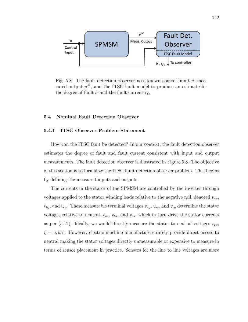
142

Fig. 5.8. The fault detection observer uses known control input u, mea-sured output yM , and the ITSC fault model to produce an estimate forthe degree of fault σ and the fault current ifs.

5.4 Nominal Fault Detection Observer

5.4.1 ITSC Observer Problem Statement

How can the ITSC fault be detected? In our context, the fault detection observer

estimates the degree of fault and fault current consistent with input and output

measurements. The fault detection observer is illustrated in Figure 5.8. The objective

of this section is to formalize the ITSC fault detection observer problem. This begins

by defining the measured inputs and outputs.

The currents in the stator of the SPMSM are controlled by the inverter through

voltages applied to the stator winding leads relative to the negative rail, denoted vag,

vbg, and vcg. These measurable terminal voltages vag, vbg, and vcg determine the stator

voltages relative to neutral, vas, vbs, and vcs, which in turn drive the stator currents

as per (5.12). Ideally, we would directly measure the stator to neutral voltages vζs,

ζ = a, b, c. However, electric machine manufacturers rarely provide direct access to

neutral making the stator voltages directly unmeasurable or expensive to measure in

terms of sensor placement in practice. Sensors for the line to line voltages are more

143

readily available, i.e. measurements of vζw � vζs − vws for ζ = w ∈ {a, b, c}. The line

to line voltages are measurable from the controlled voltages vag, vbg, and vcg as per

vMab = vMag − vMbg

vMbc = vMbg − vMcg

vMac = vMag − vMcg ,

(5.18)

where the superscriptM denotes measured signals. We also consider the electrical po-

sition θr and speed ωr of the rotor to be measured signals. Using these measurements,

the back emf eabcf can be expressed as⎡⎢⎢⎢⎢⎢⎢⎣ea

eb

ec

ef

⎤⎥⎥⎥⎥⎥⎥⎦ =

⎡⎢⎢⎢⎢⎢⎢⎣1− σ 0 0

0 1 0

0 0 1

σ 0 0

⎤⎥⎥⎥⎥⎥⎥⎦⎡⎢⎢⎢⎣

ωMr λm cos(θMr )

ωMr λm cos(θMr − 2π/3)

ωMr λm cos(θMr + 2π/3)

⎤⎥⎥⎥⎦ . (5.19)

Note that the only unknown in (5.19) is σ, which is estimated. Thus the rightmost

matrix in (5.19) becomes another measured input.

Since many commercial electric drive systems utilize stator current control, sensors

are often available for the stator currents iζs, ζ = a, b, c. We assume that each of the

stator currents is available for measurement. In practice, we can reduce the number of

sensors since the stator currents satisfy Kirchoff’s current law, i.e., ias + ibs + ics = 0.

One may be able to use a reduced number of sensors, but this reduction is not explored

in this chapter.

When an ITSC fault occurs, the same voltage potential on the phase terminals

produces different stator current responses. Essentially, the ITSC fault detection

observer matches the given voltage signals to the resulting current measurements to

determine the degree of fault σ, the fault current ifs, and the stator currents iζs,

ζ = a, b, c. We can now pose the ITSC fault observer problem.

ITSC Observer Problem: Estimate the fault severity σ, fault current ifs, and

stator currents iζs, ζ = a, b, c, given the ITSC fault model (5.12), measured signal

yM =[vMab vMbc vMca iMas iMbs iMcs

]�, (5.20)

144

and known electrical rotor speed ωMr and position θMr where the superscriptM denotes

measured variables.

ITSC fault detection is a nonlinear observer problem. For each fixed degree of

fault σ, the dynamics in (5.12) are linear with respect to iabcf , but an unknown de-

gree of fault σ introduces a nontrivial nonlinearity. One approach to solving nonlinear

observability problems is to use linear observers, such as the classical Luenberger dy-

namical observer [58]. Linear observers are numerically simple and well understood,

but in general perform poorly on highly nonlinear systems. As an alternative, we pro-

pose the optimization-based approach developed in [22], known as a moving horizon

estimator or moving horizon observer (MHO).

5.4.2 Moving Horizon Observer

As mentioned in the introduction, the MHO re-poses the estimation problem as

an optimization problem. Consider the following nonlinear system

x = f(x, uM)

yM = g(x, uM),(5.21)

where x ∈ Rn is the state, yM ∈ R

p is the measured output, uM : R → Rm is

the bounded measurable input, and f : Rn × Rm → R

n and g : Rn × Rm → R

p

are known, locally Lipschitz functions with respect to both x and uM . Recall that

for A, B metric spaces, h : A → B is a locally Lipschitz function if for all a ∈ Athere exists a neighborhood Ua of a and a constant K such that for all a1, a2 ∈ Ua,

‖h(a1) − h(a2)‖A ≤ K‖a1 − a2‖B, where ‖ · ‖A and ‖ · ‖B denote the metric in A

145

and B, respectively. The MHO developed in [22] is based on solving the optimization

problem

minx0∈Rn

∫ t

t−T

‖yM(t)− y(t)‖2dt (5.22)

subject to:

˙x(t) = f(x(t), uM(t)), x(t− T ) = x0 (5.23)

y(t) = g(x(t), uM(t)). (5.24)

where T is the finite horizon and y(t) is the estimated output driven by the state

trajectory x(t) which satisfies the underlying differential equation with the estimated

initial condition x0. The specific approach in [22] is not to solve (5.22) at each time

t but rather to sequentially solve the optimization over successive horizon windows

[tk − T, tk] where t1 < t2 < t3 < · · · . However, our approach is not to achieve the

absolute minimum over [tk − T, tk], but rather to impose a cost reduction by a factor

of β ∈ (0, 1) from one window to the next. So if at time tk, the norm in (5.22) is equal

to Kk, then over the next horizon [tk+1−T, tk+1] the minimization in (5.22) is iterated

until the norm is less than Kk+1 = βKk. This would continue until the norm in (5.22)

is in a sufficiently small neighborhood of zero, in which case yM(t) − y(t; x0) ≈ 0.

Given the presence of modeling errors, sensor noise, and numerical round-off, reaching

the “perfect minimum” of zero is unlikely. The benefit of this approach is that

the observer/estimate convergence improves incrementally over successive horizons in

contrast to the larger computational effort needed to achieve the minimum of (5.22)

over each horizon.

To guarantee solvability of the observer problem, it is assumed that for each

initial condition x0, x′0 ∈ R

n, the corresponding output trajectories y(x(t), u(t)) and

y(x′(t), u(t)) satisfy∫ t

t−T

‖y(x(t), u(t))− y(x′(t), u(t))‖2dt ≥ γ‖x0 − x′0‖2, (5.25)

for some fixed γ > 0. This uniform observability condition reduces to the classical

observability Gramian in the case of time-varying linear systems and time-invariant

146

linear systems as shown in Appendix B. The uniform observability condition in (5.25)

is difficult to verify for nonlinear systems. As mentioned earlier, for the ITSC fault

detection problem we will presume that the unfaulted state model is observable, which

is easily verified for the parameter values of a typical SPMSM and available sensor

measurements. Further as asserted earlier, the faulted model is observable for almost

all fault levels σ ∈ [0, 1] if observable for at least one fault level σ1. Hence, the

structure of the SPMSM model allows us to assert generic observability of the system

without having to verify the condition of (5.25).

In general, the MHO is a versatile observer often used to solve nonlinear ob-

servability problems [22, 59, 60]. Thus it is well suited for the ITSC fault detection

problem. For linear state models, the MHO can be seen as a dual problem to the

linear quadratic regulator (LQR) problem and thus enjoys a similar historical suc-

cess [48, 61].

5.4.3 ITSC Observability

Recall that for the ITSC fault detection problem, the variables to be estimated

are the stator currents iws, w = a, b, c, f , and the degree of fault σ. First we validate

that the observability problem is feasible, i.e., different fault levels are distinguishable

and the stator currents iws are observable.

To analyze the distinguishability of two degrees of fault σ1 = σ2 ∈ [0, 1], we first

need to construct a switched linear time-invariant (SLTI) model that incorporates

the measured signals in (5.20) and then verify distinguishability with (5.4). Unfor-

tunately, only the line-to-line voltages vab, vbc, and vca are measurable whereas the

stator voltages vas, vbs, and vcs, that appear in the state dynamics of (5.12) are not.

Another problem with (5.12) is that Kirchoff’s current law (KCL) disallows arbitrary

initial conditions, because in the wye configuration ias + ibs + ics = 0. This means

that (5.12) contains redundant information and a lower dimensional state model can

capture all the relevant dynamical information.

147

To construct the lower dimensional state model (4th order to 3rd order) that utilizes

the measured signals in (5.20), we do the following:

1. using KCL, substitute ics = −ias − ibs in (5.12), i.e., for iabf � [ias, ibs, ifs]�

iabcf =

⎡⎢⎢⎢⎢⎢⎢⎣1 0 0

0 1 0

−1 −1 0

0 0 1

⎤⎥⎥⎥⎥⎥⎥⎦ iabf �Mabf iabf (5.26)

2. premultiply both sides of (5.12) by

Mv �

⎡⎢⎢⎢⎣1 −1 0 0

0 1 −1 0

0 0 0 1

⎤⎥⎥⎥⎦ (5.27)

to obtain differential equations as functions of (i) vMab = vas − vbs and (ii) vMbc =

vbs − vcs.

This results in the reduced-order equivalent state and output model:

Lf (σ)d

dtiabf = −Rf (σ)iabf + Q(σ)uM , (5.28)

yM =

⎡⎣1 0 0

0 1 0

⎤⎦ iabf � C(σ)iabf , (5.29)

where iabf � [ias, ibs, ifs]� is the reduced state vector. The measured input vector is

uM =[λmω

Mr cos(θMr ) λmω

Mr cos(θMr − 2π/3) λmω

Mr cos(θMr + 2π/3) vMab vMbc

]�,

(5.30)

148

and the measured output is yM = [ias, ibs]�. The new linear system matrices in (5.28)

are

Lf (σ) =MvLf (σ)Mabf ,

Rf (σ) =Mv

⎡⎢⎢⎢⎢⎢⎢⎣(1− σ)Rs 0 0 0

0 Rs 0 0

0 0 Rs 0

0 0 0 σRs

⎤⎥⎥⎥⎥⎥⎥⎦Mabf ,

Q(σ) =

⎡⎢⎢⎢⎣−(1− σ) 1 0 1 0

0 −1 1 0 1

−σ 0 0 0 0

⎤⎥⎥⎥⎦ ,where Mabf and Mv are defined in (5.26) and (5.27), respectively.

To verify the fault distinguishability conditions in (5.4), a standard LTI system

is constructed from (5.28) for each degree of fault σ1 via the tuple of linear system

matrices

(Aσ1 , Bσ1 , Cσ1 , Dσ1) =(L†f (σ1)Rf (σ1), L

†f (σ1)Q(σ1), C(σ1), 0

). (5.31)

If there exists two degrees of fault σ1 = σ2, for which (5.4) is satisfied, then (for generic

inputs) almost all degrees of fault are distinguishable. For the SPMSM parameterized

in Table 5.1 with σ1 = 0 and σ2 = 1, we compute

‖Γ2n(Aσ1 , Bσ1 , Cσ1 , Dσ1)− Γ2n(Aσ2 , Bσ2 , Cσ2 , Dσ2)‖2F = 3.16× 1020 = 0. (5.32)

Thus σ1 = 0 and σ2 = 1 are distinguishable for almost all inputs, as per [18]. To show

that almost all degrees of fault are distinguishable for almost all inputs, we consider

the nontrivial polynomial (nontrivial by (5.32)) in σ1 and σ2 defined by (5.33),

‖Γ2n(Aσ1 , Bσ1 , Cσ1 , Dσ1)− Γ2n(Aσ2 , Bσ2 , Cσ2 , Dσ2)‖2F . (5.33)

Hence, the set of pairs (σ1, σ2) such that (5.33) is equal to zero is an algebraic variety of

lower dimension, i.e., at worst unions of lines in R2. In addition, this algebraic variety

149

must intersect the square [0, 1]× [0, 1] for two degrees of fault to be indistinguishable.

Thus it is possible that the algebraic variety does not intersect [0, 1]× [0, 1] for pairs

(σ1, σ2) with σ1 = σ2, i.e., that all degrees of fault are distinguishable. Hence for

generic inputs it follows that almost all degrees of fault are, in fact, distinguishable.

The next question is whether the state iabf is observable once the correct degree

of fault is identified. This is verified using classical observability tests on the pair

(Aσi, Cσi

), such as the rank of the observability matrix. For the SPMSM parametrized

in Table 5.1 with σ1 = 0 and σ2 = 1, we obtain

rank[O3(Aσ1 , Cσ1)] = 2

rank[O3(Aσ2 , Cσ2)] = 3,

where O3(A,C) is the observability matrix for the pair (A,C), i.e.,

Oi(A,C) =[C� (CA)� · · · (CAi−1)�

]�.

The result that rank[O3(Aσ1 , Cσ1)] = 2 implies that the state iabf is not completely

observable. This is understandable since σ1 = 0 represents the unfaulted SPMSM

and the fault current ifs is unobservable because it is zero prior to an ITSC fault.

On the other hand, since rank[O3(Aσ2 , Cσ2)] = 3, the entire state iabf is observable

for σ2 = 1. Using the same arguments as in Section 55.1.5, this implies that iabf is

observable for almost all degrees of fault. Mathematically, the set of degrees of fault

σ for which iabf is unobservable is among a finite set of roots to a polynomial in σ.

Any root, say σ∗ ∈ [0, 1] is not a physically realizable degree of fault. Hence, it is

again possible that the current iabf is observable for all degrees of fault and in the

worst case iabf is unobservable for a finite number of degrees of fault. Thus the ITSC

observer problem is feasible for almost all degrees of fault.

5.4.4 Nominal ITSC Observer

Although it is possible to build a MHO for the reduced order model of the previous

section, from a modeling perspective as well as a more direct utilization of the full

150

order model developed earlier, we simply add the KCL equation as a constraint. There

are also numerical advantages due to the sparseness of the larger set of equations.

Since the degree of fault is unknown but takes values in the interval [0, 1], we

denote the observer below to be the nominal embedded moving horizon observer

(EMHO).2 As mentioned earlier, we assume that the ITSC fault occurs in phase-a.

Relaxing this assumption is a straightforward extension, but the additional notation

is not included for clarity.

In the EMHO framework, the ITSC fault detection problem has mode σ ∈ [0, 1]

and state iabcf � [ias, ibs, ics, ifs]�. As described in Section 5.4.2, we consider a dis-

cretized set of final times given by t1, t2, · · · , tk, · · · . For simplicity, we consider evenly

spaced final times, i.e., tk+1 − tk = Tshift.

So for a given horizon [tk − T, tk] and 0 ≤ h ≤ T , the nominal ITSC fault EMHO

problem with fault in phase-a is given by

miniabcf (tk−h)∈R4

σ:[tk−T,tk]→[0,1]

∫ tk

tk−T

‖yM(t)− y(t)‖2dt (5.34)

subject to:

vabcf = Rf (σ)iabcf + Lf (σ)d

dtiabcf + eabcf (σ) (5.35)

y = [vas − vbs, vbs − vcs, vcs − vas, ias, ibs, ics]� (5.36)

= [vab, vbc, vca, ias, ibs, ics]�

0 = ias + ibs + ics, (5.37)

3 where (5.37) is a result of KCL,

iabcf = [ias, ibs, ics, ifs]�, (5.38)

vabcf = [vas, vbs, vcs, 0]�, (5.39)

2This formulation is the dual to the embedded hybrid optimal control problem in that σ can varycontinuously in [0, 1] (see [12, 61]).3Kirchoff’s current law takes the form of (5.37) only for ITSC faults, i.e., (5.37) only applies forshorts between phases and not shorts to ground. Modeling shorts to ground are not considered inthis chapter.

151

Rf (σ) =

⎡⎢⎢⎢⎢⎢⎢⎣(1− σ)Rs 0 0 0

0 Rs 0 0

0 0 Rs 0

0 0 0 σRs

⎤⎥⎥⎥⎥⎥⎥⎦ (5.40)

Lf (σ) =

⎡⎢⎢⎢⎢⎢⎢⎣(1− σ)2L (1− σ)M (1− σ)M σ(1− σ)L

(1− σ)M L M σM

(1− σ)M M L σM

σ(1− σ)L σM σM σ2L

⎤⎥⎥⎥⎥⎥⎥⎦ , (5.41)

and

eabcf (σ) = ωrλm

⎡⎢⎢⎢⎢⎢⎢⎣(1− σ) cos(θr)

cos(θr − 2π/3)

cos(θr + 2π/3)

σ cos(θr)

⎤⎥⎥⎥⎥⎥⎥⎦ . (5.42)

Of course, this problem is solved sequentially for each interval [tk − T, tk] for k =

1, 2, · · · . It is not necessary that these intervals be disjoint. As we will see in the

forthcoming development, there are numerical advantages to having these intervals

overlap.

Several aspects of the ITSC EMHO warrant explanation and elaboration. First,

the variable h allows for the estimated state iabcf (tk − h) to be anywhere within

the interval [tk − T, tk]. For example, when h = T the EMHO observer reduces to

the MHO observer described in Section 5.4.2, in that one is estimating the initial

condition iabcf (tk − T ) for the interval [tk − T, tk]. Another way of saying this is that

the state estimate at the beginning of the interval, iabcf (tk − T ), is either a delayed

estimate of the current state iabcf (tk) or must be integrated using (5.12). This value

could be sensitive to errors in the estimated initial condition. Clearly, then the choice

of h has an effect on the numerical implementation of the EMHO.

Moving the state estimate to the beginning of the interval, h small, has a smaller

delay and less integration required to obtain the current estimate. Thus, small h nat-

urally emphasizes the most recent measurements and adapts more quickly to changes

152

in the measured output. However, if h < Tshift, where Tshift = tk+1 − tk for each

k, then tk+1 − h is not contained in the previous interval [tk − T, tk] as illustrated in

Figure 5.9. The practical consequence of selecting h < Tshift occurs when integrat-

ing the previous estimate iabcf (tk − h) from tk − h to tk+1 − h to hot-start the next

estimate iabcf (tk+1 − h). Namely, the issue is that when computing iabcf (tk − h) and

σ([tk − T, tk]), no measurements from the interval [tk, tk+1 − h] were utilized. Conse-

quently, one either makes assumptions about the interval [tk, tk+1−h] to allow for the

integration (such as assuming the degree of fault σ does not change) or uses another

suboptimal initial guess (such as using iabcf (tk) to hot-start iabcf (tk+1 − h)). As pass-

ing the previous estimate forward to the next interval is critical for fast algorithm

convergence, we further restrict h to be greater than Tshift, i.e., Tshift ≤ h ≤ T .

A second point to be made is that if there is a short to ground, then (5.37) is not

valid because a short to ground allows some of the current to circumvent the neutral

node in the stator windings. Thus we disallow shorts to ground in this discussion.

Thirdly, the minimization over σ : [tk − T, tk] → [0, 1] denotes searching for all

functions σ with domain [tk − T, tk] and range in [0, 1]. The nominal ITSC EMHO

problem requires an optimization of iabcf (tk−h) ∈ R4 and σ over functions with range

in [0, 1]. What has not been utilized in (5.34)-(5.37), is the steady state behavior

inherent in the ITSC observer problem described in Section 5.4.1. The exploitation

of the steady state behavior significantly reduces computation as discussed in the

following section.

Finally, if the estimates iabcf (tk −h) = iabcf (tk −h) and σ are exact, then the cost

function in (5.34) is zero since both the estimates and actual stator currents would

be solutions to the same differential equations and have the same output function.

Since (5.34) is nonnegative, the correct estimates are a minimizing solution to the

cost function. If the only solution to (5.34) is the correct stator current and degree

of fault, the observer problem is feasible. Feasibility has been discussed theoretically

in Section 5.4.3 and demonstrated through simulation to follow.

153

Fig. 5.9. (A) and (B) illustrate how the previous horizon estimate iabcf (tk−h1) is integrated forward to hot-start iabcf (tk+1 − h1) when h1 ≥ Tshift.Notice, that the integration is within the interval [tk −T, tk]. (C) and (D)illustrate when h2 < Tshift. Note, that the integration is not contained in[tk − T, tk].

154

5.5 Practical Observer Implementation

The time constants associated with the stator currents in the SPMSM are much

faster than (i) changes in the mechanical load and (ii) changes in the voltage or

power commands. As a result, our analysis presupposes that the stator currents

and voltages are in steady-state. Specifically, the steady-state stator currents and

voltages are assumed to exhibit periodic sinusoidal behavior with frequency ωr due

to the sinusoidal back emf eabcf . Note, this sinusoidal steady-state behavior occurs

pre and post ITSC fault since in both cases the back emf eabcf is sinusoidal.

How can we exploit the steady-state periodic sinusoidal behavior of the pre and

post fault SPMSM to simplify the optimization problem in (5.34)? The approach is

to explicitly impose the structure that iζs, ζ = a, b, c, f , are sinusoids with constant

magnitudes and phase over subintervals of length tpart. The estimation of iζs can

then be re-posed as estimating gains Iqζ and Idζ , ζ = a, b, c, f , as per the following

equations:

ias = Iqa cos(θr) + Ida sin(θr) (5.43a)

ibs = Iqb cos(θr − 2π/3) + Idb sin(θr − 2π/3) (5.43b)

ics = Iqc cos(θr + 2π/3) + Idc sin(θr + 2π/3) (5.43c)

ifs = Iqf cos(θr) + Idf sin(θr). (5.43d)

How does (5.43) simplify the optimization problem in (5.34)? The primary simplifica-

tion is when solving the differential equation in (5.35). With stator and fault current

estimates with the form of (5.43), the derivatives ddtiζs, ζ = a, b, c, f , have the analytic

form

d

dtias = −Iqaωr sin(θr) + Idaωr cos(θr) (5.44a)

d

dtibs = −Iqbωr sin(θr − 2π/3) + Idbωr cos(θr − 2π/3) (5.44b)

d

dtics = −Iqcωr sin(θr + 2π/3) + Idaωr cos(θr + 2π/3) (5.44c)

d

dtifs = −Iqfωr sin(θr) + Idfωr cos(θr). (5.44d)

155

Hence, the differential equation in (5.35) can be replaced with an algebraic equation

(with respect to estimated variables Iqζ and Idζ , ζ = a, b, c, f). This greatly reduces

the complexity and computational time required to compute y in the cost function.

To apply the assumption that the stator currents are fixed sinusoids over intervals

of length tpart, we subdivide each horizon [tk − T, tk] into npart partitions of width

tpart. We assume here that the horizon length T is a scalar multiple of tpart. With

these partitions, the modified version of the ITSC EMHO estimates gains I(i)qζ and

I(i)dζ , ζ = a, b, c, f , for each partition i = 1, 2, · · · , npart of [tk − T, tk].

The partitioning of the interval [tk − T, tk] is also used to simplify estimating the

degree of fault σ(t). From a physical prospective, the ITSC faults occur when there

is a electrical short between two locations within a stator winding. This electrical

insulation failure happens at specific points and tends to have a binary behavior, i.e.,

short or no short. Consequently, the degree of fault σ(t) is expected to be piecewise

constant. This is exploited by considering the estimate σ to be constant over each

partition of the interval [tk − T, tk].

Over each partition of [tk − T, tk], the last row of (5.35) becomes an algebraic

equality constraint on the fault current estimate with respect to the gains Iqf and Idf .

This equality constraint is implemented in the simulation using a penalty function

approach, i.e., adding a penalty function of the form∫ tk

tk−T

wp‖vfs‖2dt, (5.45)

to the cost function of (5.34). Here wp ∈ R+ is a large weight and vfs is the last row

of (5.35), i.e.

vfs = Rsifs + σ2Ld

dtifs + σM

d

dtibs + σM

d

dtics + σ(1− σ)L

d

dtias + ef , (5.46)

with derivatives given in (5.44). Note that a feasible estimate for ifs will satisfy

vfs ≡ 0. Any nonzero value vfs is penalized by the term in (5.45).

Another adaptation of the cost function in (5.34) is to add a positive definite

weight matrix Q ∈ R6×6 to weight the output tracking error yM − y. With Q, the

156

observer can be tuned to place the largest weight on a set of outputs which most

directly affects the observability of the degree of fault σ. The modified cost function

then has the form ∫ tk

tk−T

((yM − y

)�Q(yM − y

)+ wp‖vfs‖2

)dt. (5.47)

Incorporating the above ideas into the cost function over each horizon [tk −T, tk],

the practical version of the ITSC EMHO is

minI(i)qζ ,I

(i)dζ ,σ

(i)

ζ=a,b,c,fi=1,··· ,npart

∫ tk

tk−T

((yM − y

)�Q(yM − y

)+ wp‖vfs‖2

)dt

subject to: (5.35)–(5.44), (5.46).

(5.48)

The superscript (i) denotes the ith partition of [tk − T, tk]. The constraints (5.35)–

(5.44), and (5.46) are understood to apply to each partition.

Finally, to simplify the transition from one optimization problem to the next, the

horizon is always uniformly shifted forward in time by tpart, i.e., tk+1 = tk+tpart. This

allows one last important modification to the ITSC EMHO concerning how estimates

in preceding horizons are used to initialize or “hot-start” subsequent optimization

problems. The scheme is illustrated in Figure 5.10. The method of partitioning each

optimization horizon evenly has the advantage that estimates in some partitions of

a previous horizon coincide with estimates of the current horizon. The partition

[tk+1 − tpart, tk+1] does not coincide with the previous partition estimates. Thus, the

estimate for [tk− tpart, tk] is used to initialize the partition [tk+1− tpart, tk+1] as shown

in Figure 5.10.

5.6 Simulation Results

This section demonstrates the effectiveness of the ITSC EMHO. The three-phase

SPMSM considered in this simulation has parameters given in Table 5.1. The SPMSM

is simulated over [0, 1] according to the following scenario: i) the rotor speed is a

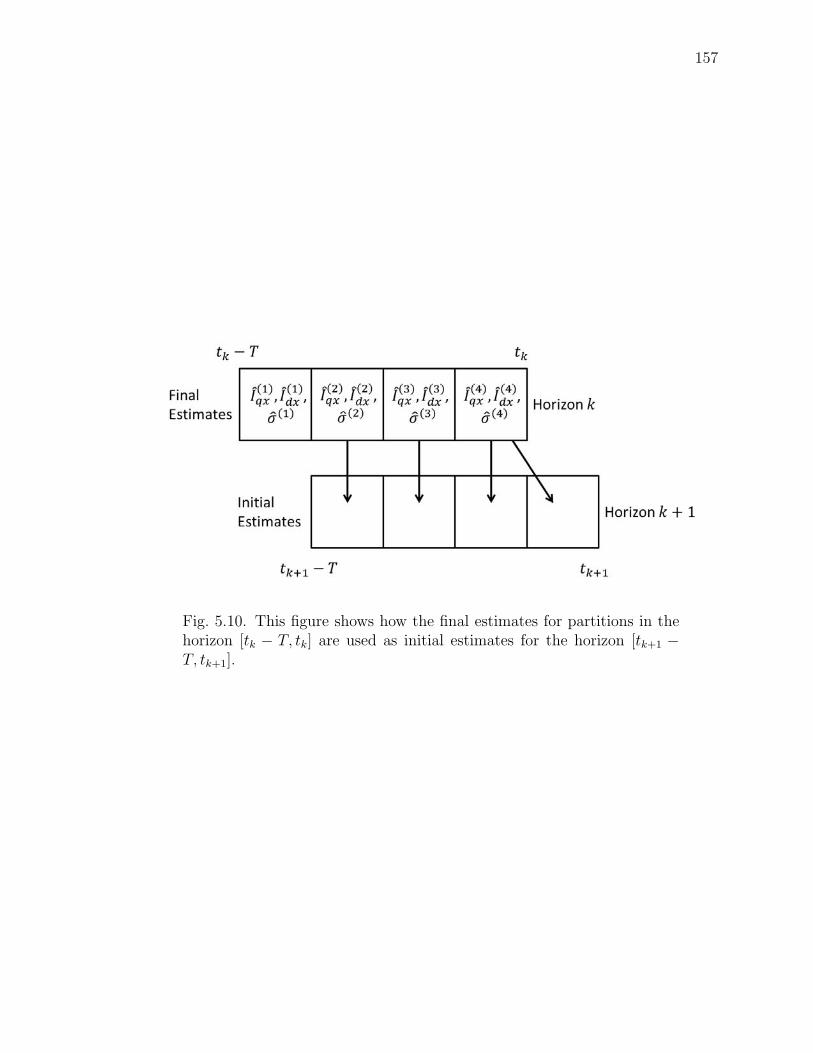
157

Fig. 5.10. This figure shows how the final estimates for partitions in thehorizon [tk − T, tk] are used as initial estimates for the horizon [tk+1 −T, tk+1].

158

constant ωm = 700 rpm, ii) using current control the stator current (before and after

fault) over [0, 1] satisfies (current in Amperes)

ias = 50 cos(θr)

ibs = 50 cos(θr − 2π/3)

ics = 50 cos(θr + 2π/3),

(5.49)

and iii) a fault of severity σf occurs at tfault = 0.5s, i.e. σ(t) = 0 for t ∈ [0, 0.5) and

σ(t) = σf for t ∈ [0.5, 1]. The scenario is simulated in MATLAB R2014b to construct

the outputs

yM =[vMab vMbc vMca iMas iMbs iMcs

]�,

where the line to line voltages vab = vas − vbs, vbc = vbs − vcs, and vca = vcs − vas are

computed using (5.12) given that the stator currents satisfy (5.49). To simulate the

fault current ifs, the differential equation in the last line of (5.12) is integrated using

the ode23t function in MATLAB with the default integration settings. For EMHO

implementation, the output yM is sampled at a rate of dt = 0.1ms.

Table 5.1.Simulation and SPMSM Parameters

Variable Symbol Value

Self Inductance L 2.31 mH

Mutual Inductance M -1.15 mH

Magnet Strength λm 0.267 Wb

Stator Resistance Rs 137 mΩ

Poles np 8

Bus Voltage Vbus 500 V

Rotor Speed ωm 700rpm

Fault Time tfault 0.5s

Simulation Step Size dt 0.1ms

159

The simulated ITSC EMHO has a horizon T = 50ms and two partitions of equal

width, i.e. tpart = 25ms. The ITSC EMHO parameters are summarized in Table 5.2.

To emphasize tracking the line to line voltage equations over stator current tracking,

a weighting matrix Q ∈ R6 is added to the cost function, i.e. the cost function is

given by ∫ t1

t1−T

(yM(t)− y(t)

)�Q(yM(t)− y(t)

)dt, (5.50)

where Q = diag(10, 10, 10, 1, 1, 1). In addition, to enforce the constraint that ifs

satisfies the last row of (5.12), we add to the cost function (5.50) a penalty function

of the form ∫ t1

t1−T

wp‖vfs‖2dt,

where wp = 1000 and vfs represents the last row on the right-hand side of (5.12), i.e.

vfs � σRsifs + σ(1− σ)Ld

dtias + σM

d

dtibs + σM

d

dtics + σ2L

d

dtifs + ef (σ).

If iabcf and σ are consistent with (5.12), vfs ≡ 0. As described in Section 5.5, the

penalty function is used as an alternative method for enforcing this equality con-

straint.

Table 5.2.ITSC EMHO Parameters

Variable Symbol Value

Number of Partitions npart 2

Horizon Width T 50ms

Partition Width tpart 25ms

The estimation error for reconstructing the fault current, i.e. |ifs − ifs| is shownin Figure 5.11 for four different degrees of fault σf = 0.01, 0.02, 0.05, 0.1. The error

|ifs − ifs| is scaled by max(ifs) which represents the amplitude of the steady state

fault current ifs for each degree of fault σf . The estimation error for reconstructing

160

0 0.2 0.4 0.6 0.8 1

|ifs−

ˆ i fs|/max

(ifs)

0

0.5

1Normalized Fault Current Estimation Error, |ifs − ˆifs|/max(ifs)

σf = 0.01σf = 0.02

time (s)0 0.2 0.4 0.6 0.8 1

|ifs−

ˆ i fs|/max

(ifs)

0

0.5

1σf = 0.05σf = 0.1

Fig. 5.11. The fault current reconstruction error |ifs− ifs| is simulated forfour levels of fault, σf = 0.01, 0.02, 0.05, and 0.1. The figure is normal-ized by max(ifs) which represents the magnitude of the steady state faultcurrent ifs for each degree of fault. In each simulation, the fault occursat 0.5s.

the degree of fault is shown in Figure 5.12 for each of the four different degrees of

fault σf . The estimation error for ias, ibs, and ics are not included since these are also

measured variables and hence the estimation error is on the order of 10−6 (tolerance

of the optimization).

It is clear from Figure 5.11, that after one partition of 25ms, the fault current

estimate ifs is within 5% of the actual fault current ifs. Similarly, the degree of fault

estimation error is within 0.001 after one partition of 25ms as shown in Figure 5.12.

This “bump” in the estimates right after the fault occurs is caused by an initial guess

which is far from the new level of fault. However, the next optimization window

improves the estimate of the degree of fault and fault current and converges quickly.

161

time (s)0 0.2 0.4 0.6 0.8 1

|σ−σ|

0

0.01

0.02

0.03

0.04

0.05Fault Estimation Error, |σ − σ|

σf = 0.01σf = 0.02σf = 0.05σf = 0.1

Fig. 5.12. The degree of fault reconstruction error |σ− σ| is simulated forfour levels of fault, σf = 0.01, 0.02, 0.05, and 0.1. In each simulation, thefault occurs at 0.5s.

162

The ability to improve on the previous estimates is a consequence of the manner in

which estimates from previous partitions are used to “hot-start” subsequent parti-

tions. The reader can recall that the initial states are passed from one partition to

hot-start the next as illustrated in Figure 5.10.

The ITSC EMHO has additional applications beyond fault detection. One such

application is fault-tolerant control schemes where the estimate for the degree of

fault can be used to determine “safe” operating conditions after a fault has occurred.

The next section explores a fault-tolerant power flow control application for a hybrid

electric vehicle, such as the Toyota Prius. This fault detection scheme also has appli-

cations for both fault detection and fault mitigating control in heavy hybrid vehicles.

The application to heavy hybrid vehicles is discussed in Section 5.7.

5.7 Application: Heavy Hybrid Vehicles

According to Harrington and Krupnick at Resources for the Future, the National

Highway Traffic Safety Administration mandated the first-ever federal requirements

for improving fuel economy in heavy-duty commercial vehicles in 2011 [65]. The focus

on reducing fuel consumption in heavy vehicles on the highway has also had an impact

in the off-road heavy vehicle industry. Leading companies of off-road vehicles, such

as Caterpillar and John Deere, have released hybrid versions of off-road construction

and forestry equipment. Although fuel prices have dropped in the past few years, the

environmental, economic, and regulatory influences on heavy vehicle design promise

continued growth in the area of heavy hybrid technology.

Electric machines are a common component in heavy hybrid vehicles, such as the

Caterpillar D7E Dozer [66] and the John Deere 644k Hybrid Wheel Loader [67]. The

Deere 644k Hybrid Wheel Loader uses two permanent-magnet synchronous machines

(PMSM), one primarily as a generator and the other as a transmission drive. Due to

the tough working conditions of these vehicles, the areas of safety, robust performance,

and reduced repair costs are key marketable features. In the event of a fault within

163

the electric machine, fault detection, and fault-tolerant control in the heavy hybrid

vehicles can improve each of these marketable features. The detection of an inter-

turn short circuit (ITSC) fault in the stator windings of the PMSM is critical to

maintaining the safe operation of these vehicles. In this section we outline the impact

of this work on ITSC fault detection in PMSM to the industry of heavy hybrid

vehicles.

5.7.1 Increased Scale

The simulation in Section 5.6 demonstrates the effective use of the ITSC fault

detection scheme using an embedded moving horizon observer (EMHO). The surface

PMSM (SPMSM) explored in Section 5.6 has a maximum power of about 30kW.

Heavy hybrid drivetrains require motors on the scale of hundreds of kilowatts. Fortu-

nately, the size of the motors does not effect the structure of the mathematical model

for SPMSM or the structure of the EMHO used to detect ITSC faults. As such,

the same techniques developed for ITSC fault detection for SPMSM can be applied

directly to SPMSM in heavy hybrid vehicles.

5.7.2 Interior PMSM

Many heavy hybrid vehicle manufacturers prefer interior PMSM (IPMSM) over

the surface mounted counterparts. Although the control of SPMSM is simpler, the

IPMSM has manufacturing advantages as well as some additional control techniques.

The magnets in the IPMSM are embedded in the rotor laminations. This allows

for permanent magnets which are rectangular and easier to produce in addition to

avoiding the problem of attaching magnets to the surface of the rotor. Another key

advantage to the IPMSM, is that the iron in the rotor can be magnetized between the

magnetic poles and provide the so-called reluctance torque. The reluctance torque is

especially useful at producing power at high speeds when the bus voltage limits the

output power. Despite the advantages of the IPMSM, stators in IPMSM and SPMSM

164

are similar and can suffer from the same ITSC winding faults. In this subsection, we

will introduce a stator voltage model from the IPMSM and discuss the applications

of the SPMSM fault detection work.

The unfaulted interior PMSM (neglecting leakage inductance) can be modeled

by [51]

vabc = Rsiabc +d

dt[LAB(θr)iabc] + eabc (5.51)

where vabc = [vas, vbs, vcs]�, iabc = [ias, ibs, ics]

�, Rs denotes the stator resistance in

each coil, θr and ωr are the electrical position and speed of the rotor, the back emf

eabc satisfies

eabc =

⎡⎢⎢⎢⎣ea

eb

ec

⎤⎥⎥⎥⎦ = λmωr

⎡⎢⎢⎢⎣cos(θr)

cos(θr − 2π/3)

cos(θr + 2π/3)

⎤⎥⎥⎥⎦ , (5.52)

and the inductance matrix LAB(θr) has the form

LAB =

⎡⎢⎢⎢⎣LA + LB cos 2θr − 1

2LA + LB cos 2(θr − π

3

)− 1

2LA + LB cos 2(θr +

π3

)− 1

2LA + LB cos 2(θr − π

3

)LA + LB cos 2

(θr − 2π

3

)− 1

2LA + LB cos 2(θr + π)

− 12LA + LB cos 2

(θr +

π3

)− 1

2LA + LB cos 2(θr + π) LA + LB cos 2(θr +

2π3

)⎤⎥⎥⎥⎦ .

(5.53)

In the case of the SPMSM, the sinusoidal inductance terms LB cos(·) is zero.Modeling an IPMSM with ITSC faults is an area of future research. From the

developments in Section 5.3, we expect that the back emf eabc and the inductance

matrix LAB(θr) will become functions of the degree of fault σ ∈ [0, 1]. The key

difference is modeling how LA and LB change after a fault has occured. Despite the

current lack of an ITSC fault model for the IPMSM, the fault detection framework

and observer structure can be extended to the IPMSM pending the model for the

ITSC faults. The structure for the IPMSM ITSC fault detection problem is shown in

Figure 5.13.

165

Fig. 5.13. Fault detection scheme for IPMSM with estimated degree offault σ and estimated fault current ifs.

166

5.7.3 Fault-Tolerant Control

After an ITSC fault has occurred, the eddy loop acts as an induction heater within

the stator windings. For heavy vehicles, oil-cooled stator windings improve the ability

to cool the stator windings after an ITSC fault and may allow for a reduced operating

condition for short periods of time. This reduced operating condition, or “limp-home”

mode, can allow vehicles in remote work sites to reach a safe location for repairs. Since

off-road heavy vehicles can spend considerable time in remote locales, the ability to

“limp home” provides a significant advantage.

Similar to the fault-tolerant scheme for the Prius, we propose using the ITSC

fault model of the PMSM (whether surface or interior magnets) to generate fault-

tolerant controls, operating limits, and efficiency curves at various degrees of fault

σ. The method for constructing these efficiency curves and fault-tolerant controls are

discussed in Section 5.3 and [62]. The basic structure for the fault tolerant control

with a high-level power flow controller is shown in Figure 5.14.

5.8 Future Work

In this chapter, we have developed a moving horizon observer to detect ITSC

faults in surface permanent magnet synchronous machines. A simplified version of

the observer is validated through simulation. Application to supervisory control in

heavy hybrid vehicles is also developed.

The development of an ITSC fault model for interior permanent magnet syn-

chronous machines is an area of future research. With this model, a moving horizon

observer can be developed to detect ITSC faults in much the same manner as pre-

sented in this paper. Another area of future research is validating the fault models

and fault detection scheme in physical devices. The model validation of the fault

model for surface permanent magnet machines was started in [57], but verification of

the interior permanent magnet machine fault model is still incomplete.

167

Fig. 5.14. Fault-tolerant control scheme with estimated degree of fault σand estimated fault current ifs.

168

Optimizing the computational time for the moving horizon observer is also an

area of future work. In part, this requires optimizing the number of horizons, hori-

zon width, and the search algorithm. This is a dual formulation to the problem in

model predictive control of determining optimal horizon parameters. As computa-

tional power in vehicles continues to increase and processor prices decrease, we expect

that using moving horizon observers for fault detection will become an increasingly

attractive solution to improving electric machine safety, reliability, and repair costs.

Appendix A

When an ITSC fault occurs in two phases simultaneously, say phase-a and phase-

b, there exists fault currents iafs and ibfs within each of the two fault loops. The degree

of fault in each phase is denoted σa and σb. For ease of notation we define τa = 1−σaand τb = 1− σb. The stator voltage model is given by

vabcf = Rf (σa, σb)iabcf + Lf (σa, σb)d

dtiabcf + eabcf (σa, σb),

where

vabcf =[vas vbs vcs 0 0

]�, iabcf =

[ias ibs ics iafs ibfs

]�,

Rf (σa, σb) =

⎡⎢⎢⎢⎢⎢⎢⎢⎢⎢⎣

τaRs 0 0 0 0

0 τbRs 0 0 0

0 0 Rs 0 0

0 0 0 σaRs 0

0 0 0 0 σbRs

⎤⎥⎥⎥⎥⎥⎥⎥⎥⎥⎦,

Lf (σa, σb) =

⎡⎢⎢⎢⎢⎢⎢⎢⎢⎢⎣

τ 2aL τaτbM τaM τaσaL τaσbM

τaτbM τ 2b L τbM τbσaM τbσbL

τaM τbM L σaM σbM

τaσaL τbσaM σaM σ2aL σaσbM

τaσbM τbσbL σbM σaσbM σ2bL

⎤⎥⎥⎥⎥⎥⎥⎥⎥⎥⎦,

169

and

eabcf (σa, σb) = λmωr

⎡⎢⎢⎢⎢⎢⎢⎢⎢⎢⎣

τa cos(θr)

τb cos(θr − 2π/3)

cos(θr + 2π/3)

σa cos(θr)

σb cos(θr − 2π/3)

⎤⎥⎥⎥⎥⎥⎥⎥⎥⎥⎦An ITSC fault occurs in all three phases, there is an additional fault current icfs and

degree of fault σc. The stator voltage model extends is an extension of the two-

phase stator voltage model. The electromechanical power couples the electrical and

mechanical components of the SPMSM as per the following equation

Teωm = Pa + Pb + Pc + P af + P b

f = Jωmωm +Bω2m + TLωm,

where P af = σaλmωri

afs cos(θr), P

bf = σbλmωri

bfs cos(θr − 2π/3), and Pζ = eζiζs for

ζ = a, b, c. The total inverter power, Pinv = Pinv,a + Pinv,b + Pinv,c, is given by

Pinv = τaRsi2as + τbRsi

2bs +Rsi

2cs + σaRs(i

afs)

2 + σbRs(ibfs)

2

+d

dtΥf (σa, σb) + Pa + Pb + Pc + P a

f + P bf ,

where Υf (σa, σb) = i�abcfLf (σa, σb)iabcf .

Appendix B

For the LTV system

x(t) = A(t)x(t) + B(t)u(t) (5.54)

y(t) = C(t)x(t) +D(t)u(t), (5.55)

the output y(t) can be expressed as a function of the initial state x0 and input u(t)

as per

y(t) = C(t)Φ(t, t0)x0 + C(t)

∫ t

t0

Φ(t, q)B(q)u(q)dq +D(t)u(t), (5.56)

170

where Φ(t, t0) is the state transition matrix [13]. Using (5.56), the left-hand side of

the strong observability condition in (5.25) can be expressed as∫ t

t−T

‖y(x(t), u(t))− y(x′(t), u(t))‖2dt

=

∫ t

t−T

‖C(q)Φ(q, t− T )x0 − C(q)Φ(q, t− T )x′0‖2dq

= (x0 − x′0)�WO(t, t− T )(x0 − x′0)

≥ λmin(WO(t, t− T ))‖x0 − x′0‖22

where WO(t, t−T ) is the observability Grammian for (5.54). The LTV system (5.54)

is observable over [t − T, t] if and only if the observability Grammian WO(t, t − T )

is positive definite, i.e., if and only if λmin(WO(t, t − T )) > 0 [13]. Setting γ =

λmin(WO(t, t− T )), the strong observability condition in (5.25) is thus equivalent to

observability for LTV systems.

171

6. FUTURE WORK

This thesis develops the feasibility conditions for switched systems state and mode

sequence reconstruction, a robust observability metric and algorithm, and the embed-

ded moving horizon observer (EMHO). This chapter outlines future research topics

in the area of switched system observability and observer design. This chapter is

divided into future work for robust observability and EMHO design.

6.1 Robust Observability Extensions

The P–robustness algorithm in Chapter 3, specifically Algorithm 1, requires sev-

eral assumptions that can be relaxed in the future. First, the Assumption 3.1 requires

surjectivity of LuV S . For real perturbations, S ⊂ Rn×m, surjectivity of LuV S is be-

lieved to be unnecessarily restrictive. As described in [38], surjectivity of LuV S is

sufficient for satisfying a certain regularity condition required to guarantee algorithm

convergence. However, surjectivity of LuV S may not be necessary for all P–robustness

algorithms. For example, consider when all system matrices, property matrices, and

perturbation matrices are real, i.e., M ∈ Rn×m and P ,S ⊂ R

n×m. In this case, the

singular vectors u and V of M − R − δM are real and LuV S : S → C1×(m−n+1) is

clearly not surjective. However, experimentally it appears that Algorithm 1 converges

in this case.

One possibility for relaxing the surjectivity assumption is requiring that LuV S(S)contains LuV (M − P − S). In this case, for each R ∈ P and δM ∈ S, there exists

another perturbation δM ′ ∈ S such that

LuV (M −R− δM − δM ′) = 0.

172

This is exactly the property used in steps 5 and 6 of Algorithm 1. To guarantee

convergence using the condition LuV (M −P −S) ⊂ LuV S(S) also requires modifying

the proof of the necessary conditions in Theorem 3.2, which also utilize the surjectivity

assumption.

The second assumption that can be relaxed is Assumption 3.2 which requires each

property matrix R ∈ P to be full rank, i.e., rankR = n. This assumption guarantees

that Algorithm 1 converges to a finite property matrix R∗. This condition is sufficient

but not necessary for the existence of finite optimal property matrices. One approach

to removing this restriction is to instead compute the Pmax-bounded P–robustness

problem which restricts each property matrix R to satisfy ‖R‖F ≤ Pmax. This would

allow modifying Algorithm 1 to again guarantee that R∗ is bounded and converges.

Another key area of future work is proving the rate of convergence for Algo-

rithm 1. Based on the work of [28] and [68], it is expected that the convergence

rate will be locally quadratic, given appropriate assumptions, since Algorithm 1 is

related to Newton’s Method. One apparent challenge with proving the rate of con-

vergence is connecting the difference of the Lyapunov-like energy functions Pk+1−Pk

to convergence of δMk and Rk in the presence of the adaptive weight gk.

In addition, it is believed that Algorithm 1 may be modified to compute the

smallest rank reducing perturbation δM∗ with respect to the spectral norm, i.e.,

replacing ‖δM‖F with σ1(δM) in (3.4) from Definition 3.1. Extending Algorithm 1

to include the spectral norm in addition to the Frobenius norm metric will unify the

robustness property literature. One approach may be to modify Steps 5 and 6 of

Algorithm 1 to find δMk and δMk to be the smallest matrices (with respect to the

spectral norm) such that

LuV S(δMk) = LuV (δMk −ΔRk) (6.1)

LuV S(δMk) = LuV (M −Rk −ΔRk − δMk). (6.2)

A similar modification to ΔRk to reduce σ1(δMk) will also be required. One idea

for computing the spectral norm as opposed to the Frobenius norm may be found in

173

replacing the linear operator LuV with Lu1V1 where u1 is the first lsv ofM−δMk−Rk

and V1 contains the first rsv and n+1 through m of M − δMk −Rk. The connection

between the linear operator Lu1V1S and σ1(δM) and σ1(δM) is not fully explored, but

may allow for simple and elegant generalization.

The final area for extending the P–robustness framework and algorithm is to con-

nect the distance to the nearest SMS unobservable switched system to convergence

properties for the EMHO. The distance to the nearest SMS unobservable switched

system, is clearly related to the degree of distinguishability and the class of ε-mode

distinguishing inputs (Definition 4.4). The key is to relate the extended observability

Gramian in (2.39) to the distance to the nearest SMS unobservable switched sys-

tem. The closer the switched system is to unobservable, the closer the observability

Gramian in (2.39) is to singularity which is intimately linked to EMHO convergence.

6.2 EMHO Extensions

The EMHO is a new an open topic for future research. This thesis introduced the

basic framework and a few basic convergence properties. Three main topics appear

“ripe” for future work: 1) proving convergence of the EMHO algorithm at each step,

2) extending EMHO to switched nonlinear systems, and 3) developing a robust EMHO

in the presence of disturbances and sensor noise.

Section 4.2.6 proves convergence given that at each iteration a state and mode

estimate tuple (xi+1, vk+1) satisfies

VE(xi+1, vi+1; ti, ti+1) ≤ βVE(xi, vi; ti−1, ti)) (6.3)

for a fixed β ∈ (0, 1). Although, SMS observability guarantees that such a tuple

(xi+1, vk+1) exists, the algorithm for computing this tuple is not yet specified. Exper-

imentally, optimization programs such as sequential quadratic programs and interior-

point algorithms have been used to solve for the tuple (xi+1, vk+1). It is expected that

given certain structural properties on the switched system (say SLTI for example) it

can be proven that the optimization problem to solve for the tuple (xi+1, vk+1) is

174

locally convex. Moreover, if it is locally convex then one may be able to explicitly

bound the number of iterations required to satisfy (6.3).

Another extension of the EMHO convergence is the application to switched non-

linear systems. Proving convergence for the EMHO applied to switched nonlinear

systems is nontrivial. Details of this extension are beyond the scope of this sec-

tion, but an interested reader should explore the uniform reconstructability condition

in [22, Equation 3.4].

Possibly the most practical extension to the EMHO is to consider the effect of

disturbances and sensor noise on the EMHO. In the presence of disturbances and

sensor noise, either the disturbance and sensor noise must be estimated (likely to be

intractable) or convergence to perfect state and mode estimates should be relaxed.

One such relaxation is to compute a minimum L2 output tracking error that is solv-

able, i.e., a lower bound Vmin ≤ VE(xi, vi; ti−1, ti). This lower bound Vmin represents

the level of uncertainty for state and mode reconstruction. Given the lower bound

Vmin, one can construct a bound on the mode estimation error v(ti)− v(ti) and state

tracking error e(ti) as i → ∞. Some results for switched MHO convergence in the

presence of noise can be found in [48], but the connection to the EMHO is still an

area of active research.

REFERENCES

175

REFERENCES

[1] S. Wei, M. Zefran, K. Uthaichana, and R. A. DeCarlo, “HybridModel Predictive Control for Stabilization of Wheeled Mobile RobotsSubject to Wheel Slippage,” in Proc. 2007 IEEE Int. Conf. Robot.Autom., no. April. IEEE, apr 2007, pp. 2373–2378. [Online]. Available:http://ieeexplore.ieee.org/lpdocs/epic03/wrapper.htm?arnumber=4209438

[2] S. Wei, K. Uthaichana, M. Zefran, and R. Decarlo, “Hybrid model predictivecontrol for the stabilization of wheeled mobile robots subject to wheel slippage,”IEEE Trans. Control Syst. Technol., vol. 21, no. 6, pp. 2181–2193, 2013. [Online].Available: http://ieeexplore.ieee.org/xpls/abs{ }all.jsp?arnumber=6579667

[3] S. Liu, X. Feng, D. Kundur, T. Zourntos, and K. L. Butler-Purry, “Switched sys-tem models for coordinated cyber-physical attack construction and simulation,”in 2011 IEEE 1st Int. Work. Smart Grid Model. Simulation, SGMS 2011, 2011,pp. 49–54.

[4] R. Meyer, R. DeCarlo, P. Meckl, C. Doktorcik, and S. Pekarek, “Hybrid modelpredictive power flow control of a fuel cell-battery vehicle,” in Am. ControlConf., 2011, pp. 2725–2731[1]. [Online]. Available: http://ieeexplore.ieee.org/stamp/stamp.jsp?tp={&}arnumber=5991428{&}isnumber=5989965

[5] J. Neely, S. Pekarek, R. DeCarlo, and N. Vaks, “Real-time hybrid modelpredictive control of a boost converter with constant power load,” in 2010Twenty-Fifth Annu. IEEE Appl. Power Electron. Conf. Expo. IEEE, feb 2010,pp. 480–490. [Online]. Available: http://ieeexplore.ieee.org/lpdocs/epic03/wrapper.htm?arnumber=5433628

[6] R. Vidal, A. Chiuso, S. Soatto, and S. Sastry, “Observability of Linear HybridSystems,” in Hybrid Syst. Comput. Control. Springer Berlin/Heidelberg, 2003,pp. 526–539.

[7] D. Gomez-Gutierrez, A. Ramirez-Trevino, J. Ruiz-Leon, and S. Di Gennaro,“Observability of Switched Linear Systems: A geometric approach,” in 49thIEEE Conf. Decis. Control. IEEE, dec 2010, pp. 5636–5642. [Online]. Available:http://ieeexplore.ieee.org/lpdocs/epic03/wrapper.htm?arnumber=5717936

[8] ——, “On the Observability of Continuous-Time Switched Linear SystemsUnder Partially Unknown Inputs,” IEEE Trans. Automat. Contr., vol. 57, no. 3,pp. 732–738, mar 2012. [Online]. Available: http://ieeexplore.ieee.org/lpdocs/epic03/wrapper.htm?arnumber=6007052

[9] D. Gomez-Gutierrez, S. Celikovsky, A. Ramirez-Trevino, J. Ruiz-Leon, and S. DiGennaro, “Sliding mode observer for Switched Linear Systems,” in 2011 IEEEInt. Conf. Autom. Sci. Eng. IEEE, aug 2011, pp. 725–730. [Online]. Available:http://ieeexplore.ieee.org/lpdocs/epic03/wrapper.htm?arnumber=6042494

176

[10] D. Gomez-Gutierrez, S. Celikovsky, A. Ramırez-Trevino, and B. Castillo-Toledo, “On the Observer Design Problem for Continuous-Time SwitchedLinear Systems with Unknown Switchings,” J. Franklin Inst., 2015. [Online].Available: http://linkinghub.elsevier.com/retrieve/pii/S0016003215000642

[11] A. Balluchi, L. Benvenuti, M. D. D. Benedetto, and A. L. Sangiovanni-Vincentelli, “Design of Observers for Hybrid Systems,” in Hybrid Syst. Comput.Control, ser. Lecture Notes in Computer Science, C. Tomlin and M. Greenstreet,Eds. Springer Berlin/Heidelberg, 2002, vol. 2289, pp. 76–89.

[12] S. C. Bengea and R. a. DeCarlo, “Optimal control of switching systems,”Automatica, vol. 41, no. 1, pp. 11–27, jan 2005. [Online]. Available:http://linkinghub.elsevier.com/retrieve/pii/S0005109804002237

[13] R. A. DeCarlo, Linear Systems: A State Variable Approach with Numerical Im-plementation. Englewood Cliffs, New Jersey: Prentice Hall, 1989.

[14] W. M. Wonham, Linear Multivariable Control: A Geometric Approach, 2nd ed.Springer-Verlag New York, 1979.

[15] G. Basile and G. Marro, “Controlled and conditioned invariant subspaces inlinear system theory,” J. Optim. Theory Appl., vol. 3, no. 5, pp. 306–315, 1969.

[16] ——, “On the observability of linear, time-invariant systems with unknown in-puts,” J. Optim. Theory Appl., vol. 3, no. 6, pp. 410–415, 1969.

[17] ——, Controlled and conditioned invariant subspaces in linear system theory.Prentice Hall Englewood Cliffs, 1992.

[18] M. Babaali and G. J. Pappas, “Observability of switched linear systemsin continuous time,” Hybrid Syst. Comput. Control, vol. 3414, no. March,pp. 103–117, 2005. [Online]. Available: http://www.springerlink.com/index/150UC4MJQW7AJAE9.pdf

[19] W. Rudin, Real and complex analysis, 3rd ed. New York: McGraw-Hill BookCo., 1987.

[20] S. C. Johnson, R. A. DeCarlo, and M. Zefran, “Set-transition observabilityof switched linear systems,” in 2014 Am. Control Conf. IEEE, jun 2014,pp. 3267–3272. [Online]. Available: http://ieeexplore.ieee.org/lpdocs/epic03/wrapper.htm?arnumber=6858960

[21] E. Kreindler and P. Sarachik, “On the concepts of controllability andobservability of linear systems,” Autom. Control. IEEE . . . , 1964. [Online].Available: http://ieeexplore.ieee.org/xpls/abs{ }all.jsp?arnumber=1105665

[22] H. Michalska and D. Mayne, “Moving horizon observers and observer-basedcontrol,” IEEE Trans. Automat. Contr., vol. 40, no. 6, pp. 995–1006, jun1995. [Online]. Available: http://ieeexplore.ieee.org/lpdocs/epic03/wrapper.htm?arnumber=388677

[23] C.-T. Chen, Linear System Theory and Design, 3rd ed. New York, NY, USA:Oxford University Press, Inc., 1998.

177

[24] R. Eising, “Between controllable and uncontrollable,” Syst. Control Lett., vol. 4,no. 5, pp. 263–264, jul 1984. [Online]. Available: http://linkinghub.elsevier.com/retrieve/pii/S0167691184800353

[25] M. Wicks and R. DeCarlo, “Computing the distance to an uncontrollablesystem,” IEEE Trans. Automat. Contr., vol. 36, no. 1, pp. 39–49, 1991. [Online].Available: http://ieeexplore.ieee.org/lpdocs/epic03/wrapper.htm?arnumber=62266

[26] C. Kenney and A. J. Laub, “Controllability and stability radii for companionform systems,” Math. Control. Signals, Syst., vol. 1, no. 3, pp. 239–256, oct1988. [Online]. Available: http://link.springer.com/10.1007/BF02551286

[27] M. Wicks, “Matrix rank-robustness problems in systems and control: theory andcomputation,” Ph.D. dissertation, Purdue University, 1992.

[28] M. A. Wicks and R. A. DeCarlo, “Rank Robustness of ComplexMatrices with Respect to Real Perturbations,” SIAM J. Matrix Anal.Appl., vol. 15, no. 4, pp. 1182–1207, oct 1994. [Online]. Available:http://epubs.siam.org/doi/abs/10.1137/S0895479891194297

[29] S. R. Khare, H. K. Pillai, and M. N. Belur, “Computing the radius ofcontrollability for state space systems,” Syst. Control Lett., vol. 61, no. 2, pp.327–333, feb 2012. [Online]. Available: http://linkinghub.elsevier.com/retrieve/pii/S0167691111002957

[30] S. C. Johnson and R. A. DeCarlo, “Bounding the distance to the nearest un-observable switched linear time-invariant system,” in 2015 Am. Control Conf.Chicago, IL: IEEE, 2015, pp. 1083 – 1088.

[31] J. Clotet and M. D. Magret, “Upper Bounds for the Distance between aControllable Switched Linear System and the Set of Uncontrollable Ones,”Math. Probl. Eng., vol. 2013, no. 4, pp. 1–9, 2013. [Online]. Available:http://www.hindawi.com/journals/mpe/2013/948147/

[32] G. Hu and E. Davison, “Real Controllability/Stabilizability Radius of LTISystems,” IEEE Trans. Automat. Contr., vol. 49, no. 2, pp. 254–257, feb2004. [Online]. Available: http://ieeexplore.ieee.org/lpdocs/epic03/wrapper.htm?arnumber=1266782

[33] N. K. Son and D. D. Thuan, “The structured controllability radii of higherorder systems,” Linear Algebra Appl., vol. 438, no. 6, pp. 2701–2716,mar 2013. [Online]. Available: http://linkinghub.elsevier.com/retrieve/pii/S0024379512008026

[34] S. Lam and E. J. Davison, “Computation of the Real Controllability Radius andMinimum-Norm Perturbations of Higher-Order, Descriptor, and Time-DelayLTI Systems,” IEEE Trans. Automat. Contr., vol. 59, no. 8, pp. 2189–2195, aug2014. [Online]. Available: http://ieeexplore.ieee.org/lpdocs/epic03/wrapper.htm?arnumber=6705617

[35] J. V. Burke, A. S. Lewis, and M. L. Overton, “Pseudospectral Componentsand the Distance to Uncontrollability,” SIAM J. Matrix Anal. Appl.,vol. 26, no. 2, pp. 350–361, jan 2004. [Online]. Available: http://epubs.siam.org/doi/abs/10.1137/S0895479803433313

178

[36] M. Gu, E. Mengi, M. L. Overton, J. Xia, and J. Zhu, “Fast Methodsfor Estimating the Distance to Uncontrollability,” SIAM J. Matrix Anal.Appl., vol. 28, no. 2, pp. 477–502, jan 2006. [Online]. Available:http://epubs.siam.org/doi/abs/10.1137/05063060X

[37] C. He, “Estimating the distance to uncontrollability: A fast method and aslow one,” Syst. Control Lett., vol. 26, no. 4, pp. 275–281, nov 1995. [Online].Available: http://linkinghub.elsevier.com/retrieve/pii/0167691195000233

[38] M. Wicks and R. DeCarlo, “Computing robustness of system propertieswith respect to structured real matrix perturbations,” in [1992] Proc. 31stIEEE Conf. Decis. Control. IEEE, 1992, pp. 1909–1914. [Online]. Available:http://ieeexplore.ieee.org/lpdocs/epic03/wrapper.htm?arnumber=371098

[39] B. De Moor and S. Boyd, “Analytic Properties of Singular Values and Vectors,”ESAT-SISTA Rep., vol. 28, p. 17, 1989.

[40] D. G. Luenberger, Optimization by Vector Space Methods. John Wiley & Sons,Inc., 1969.

[41] J. Brewer, “Kronecker products and matrix calculus in system theory,” IEEETrans. Circuits Syst., vol. 25, no. 9, pp. 772–781, sep 1978. [Online]. Available:http://ieeexplore.ieee.org/lpdocs/epic03/wrapper.htm?arnumber=1084534

[42] D. S. Bernstein, Matrix Mathematics: Theory, Facts, and Formulas with Appli-cation to Linear System Theory. Princeton University Press, 2005.

[43] A. J. Laub, Kronecker Products. Society for Industrial and Applied Mathemat-ics, Philadelphia, PA, 2005.

[44] T. Kato, A short introduction to perturbation theory for linear operators.Springer New York, 2012.

[45] A. Alessandri and P. Coletta, “Design of Luenberger Observers for a Class ofHybrid Linear Systems,” in HSCC ’01 Proc. 4th Int. Work. Hybrid Syst. Comput.Control, 2001, pp. 7–18.

[46] S. Pettersson, “Designing Switched Observers for Switched Systems UsingMultiple Lyapunov Functions and Dwell-Time Switching,” in Anal. Des.Hybrid Syst. 2006. Elsevier, 2006, pp. 18–23. [Online]. Available: http://linkinghub.elsevier.com/retrieve/pii/B9780080446134500070

[47] A. Tanwani, H. Shim, and D. Liberzon, “On observability for switched linearsystems: characterization and observer design,” IEEE Trans. Automat. Contr.,vol. 58, no. 4, 2013.

[48] G. Ferrari-Trecate, D. Mignone, and M. Morari, “Moving horizon estimation forhybrid systems,” IEEE Trans. Automat. Contr., vol. 47, pp. 1663–1676, 2002.

[49] J. R. Munkres, Topology, 2nd ed., ser. Featured Titles for Topology Series. Pren-tice Hall, Incorporated, 2000.

[50] M. Babaali and M. Egerstedt, “Observability of Switched Linear Systems,” inHybrid Syst. Comput. Control. LNCS. Springer Verlag, 2004, pp. 48—-63.

179

[51] P. Krause, O. Wasynczuk, S. Sudhoff, and P. Pekarek, Analysis of Electric Ma-chinery and Drive Systems, 3rd ed. Piscataway, NJ: Wiley-IEEE Press, 2013.

[52] C. Lai, A. Balamurali, V. Bousaba, K. L. V. Iyer, and N. C. Kar,“Analysis of stator winding inter-turn short-circuit fault in interior andsurface mounted permanent magnet traction machines,” in 2014 IEEETransp. Electrif. Conf. Expo. IEEE, jun 2014, pp. 1–6. [Online]. Available:http://ieeexplore.ieee.org/lpdocs/epic03/wrapper.htm?arnumber=6861775

[53] A. Gandhi, T. Corrigan, and L. Parsa, “Recent advances in modeling and on-line detection of stator interturn faults in electrical motors,” IEEE Trans. Ind.Electron., vol. 58, no. 5, pp. 1564–1575, 2011.

[54] L. Romeral, J. C. Urresty, J. R. Riba Ruiz, and A. Garcia Espinosa, “Modelingof surface-mounted permanent magnet synchronous motors with stator windinginterturn faults,” IEEE Trans. Ind. Electron., vol. 58, no. 5, pp. 1576–1585, 2011.

[55] R. T. Meyer, R. a. DeCarlo, and S. Pekarek, “Hybrid Model PredictivePower Management of a Battery-Supercapacitor Electric Vehicle,” AsianJ. Control, vol. 18, no. 1, pp. 150–165, jan 2016. [Online]. Available:http://doi.wiley.com/10.1002/asjc.553http://doi.wiley.com/10.1002/asjc.1259

[56] K. Uthaichana, R. DeCarlo, S. Bengea, S. Pekarek, and M. Zefran, “Hybridoptimal theory and predicitive control for power management in hybrid electricvehicle,” J. Nonlinear Syst. Appl, vol. 2, no. 1-2, pp. 96—-110, 2011.

[57] K.-H. Kim, D.-U. Choi, B.-G. Gu, and I.-S. Jung, “Fault model and performanceevaluation of an inverter-fed permanent magnet synchronous motor under wind-ing shorted turn and inverter switch open,” IET Electr. Power Appl., vol. 4,no. 4, p. 214, 2010.

[58] D. Luenberger, Introduction to dynamic systems: theory, models, and applica-tions. Wiley, 1979.

[59] A. Alessandri, M. Baglietto, G. Battistelli, and V. Zavala, “Advancesin moving horizon estimation for nonlinear systems,” 49th IEEE Conf.Decis. Control, pp. 5681–5688, dec 2010. [Online]. Available: http://ieeexplore.ieee.org/lpdocs/epic03/wrapper.htm?arnumber=5718126

[60] Y. Guo and B. Huang, “Moving horizon estimation for switching nonlinear sys-tems,” Automatica, vol. 49, pp. 3270–3281, 2013.

[61] S. Bengea, K. Uthaichana, M. Zefran, and R. DeCarlo, “Optimal Control ofSwitching Systems via Embedding into Continuous Optimal Control Problem,”in Control Syst. Handbook, Second Ed., W. S. Levine, Ed. CRC Press 2011,2010, ch. 31, pp. 31–1–31–23.

[62] R. T. Meyer, S. C. Johnson, R. A. DeCarlo, and S. Pekarek, “Supervisory pow-erflow control of Toyota Prius subject to stator winding faults,” In Preperation,2016.

[63] R. A. DeCarlo and R. Saeks, Interconnected Dynamical Systems, ser. Electricaland Computer Engineering. New York: CRC Press, 1981.

180

[64] R. T. Meyer, M. Zefran, and R. A. DeCarlo, “A Comparison of the EmbeddingMethod With Multiparametric Programming, Mixed-Integer Programming,Gradient-Descent, and Hybrid Minimum Principle-Based Methods,” IEEETrans. Control Syst. Technol., vol. 22, no. 5, pp. 1784–1800, sep 2014. [Online].Available: http://ieeexplore.ieee.org/lpdocs/epic03/wrapper.htm?arnumber=6733440

[65] W. Harrington and A. Krupnick, “Improving Fuel Economy in Heavy Duty Ve-hicles,” Issue Brief 12-01. Resources for the Future, Tech. Rep., 2012.

[66] Caterpillar, “D7E.” [Online]. Available: http://www.cat.com/en{ }US/products/rental/equipment/dozers/medium-dozers/18429156.html

[67] Deere & Company, “644K Hybrid Wheel Loader.” [Online]. Avail-able: https://www.deere.com/en{ }US/products/equipment/wheel{ }loaders/644k{ }hybrid/644k{ }hybrid.page

[68] M. A. Wicks and R. A. DeCarlo, “Computing Most Nearly Rank-Reducing Structured Matrix Perturbations,” SIAM J. Matrix Anal. Appl.,vol. 16, no. 1, pp. 123–137, jan 1995. [Online]. Available: http://epubs.siam.org/doi/abs/10.1137/S089547989222758X

VITA

181

VITA

Scott C. Johnson was born in Fort Wayne, Indiana in 1989. Mr. Johnson attended

grade school and high school in Caldwell, Idaho. He received a B.S. degree in Math-

ematics/Physics from The College of Idaho, Caldwell, ID in 2007. He also received

a M.S. degree in Electrical Engineering from Purdue University, West Lafayette, In-

diana. Currently he is a Ph.D. candidate at Purdue University and will receive his

degree in August 2016.

Mr. Johnson’s primary research interests include switched system observer design,

observability, and robust observers.