arX

iv:a

stro

-ph/

0204

504v

2 2

1 Ju

n 20

02

Quintessence, super-quintessence and observable quantities in Brans-Dicke and

non-minimally coupled theories

Diego F. TorresPhysics Department, Princeton University, NJ 08544, USA

The different definitions for the equation of state of a non-minimally coupled scalar field that havebeen introduced in the literature are analyzed. Particular emphasis is made upon those featuresthat could yield to an observable way of distinguishing non-minimally coupled theories from GeneralRelativity, with the same or with alternate potentials. It is found that some earlier claims on thatsuper-quintessence, a stage of super-accelerated expansion of the universe, is possible within realisticnon-minimally coupled theories are the result of an arguable definition of the equation of state. Inparticular, it is shown that these previous results do not import any observable consequence, i.e. thatthe theories are observationally identical to General Relativity models and that super-quintessenceis not more than a mathematical outcome. Finally, in the case of non-minimally coupled theorieswith coupling F = 1+ξφ2 and tracking potentials, it is shown that no super-quintessence is possible.

PACS numbers: 98.80.Cq, 98.70.Vc

I. INTRODUCTION

During the last years, observations of distant Type Iasupernovae [1] and CMB measurements [2] have shownthat the universe is, most likely, undergoing a process ofaccelerated expansion. The widespread vision of the cos-mological model is, since then, a spatially flat low matterdensity universe. This implies that the total energy den-sity today is dominated by a contribution having nega-tive pressure (cosmological constant, or quintessence [3])which has just began to undertake the leading role in theright hand side of the Einstein field equations.

The cosmological constant solution to this state of af-fairs appears not to be completely satisfactory (see forinstance [4]). Precise initial conditions should be givenin order to solve the coincidence problem (why the vac-uum energy is dominating the energy density right now).Moreover, a fine-tuning problem appears, since a vac-uum energy density of order ∼ 10−47GeV4 requires a newmass scale about 14 orders of magnitude smaller than theelectroweak scale, having no a-priori reason to exist. Inaddition, the equation of state, p/ρ, for vacuum energy isexactly equal to −1, what at first sight appears as yet an-other value which is, in a dynamical setting, precisely set.Quintessence [3], and its derived models, being the mainalternatives, are based on the existence of one or manyscalar fields, which dynamically evolve together with allothers components of the universe. The above-mentionedproblems are alleviated within this framework. A sub-class of models, those having inverse power law poten-tials, present tracking solutions where a given amount ofscalar field energy density can be reached starting froma large range of initial conditions (see for e.g. Refs. [5]).

The simplest models of quintessence are based on mini-mally coupled scalar fields. For a general potential V , theequation of state for those quintessence models is givenby

p

ρ=

φ2 − 2V

φ2 + 2V, (1)

and it can be easily proven that this expression isbounded to be within the range -1 ≤ p/ρ ≤ 1, unlessof course one is willing to accept negative defined poten-tials. In the latter cases, the energy density becomes itselfa negative quantity. For usual models of quintessence,then, it is clear that no super-acceleration can appear.The latter is a result of an extremely negative (< −1)equation of state. This possible super-accelerated ex-pansion has been recently dubbed super-quintessence byseveral authors, e.g. [6], although its consequences arebeing analyzed since some time before [7]. The main rea-son supporting this interest is that current observationalconstraints are indeed compatible with, if not favoring,such values for the equation of state (see for instance Ref.[7]).

Extended quintessence models are those in which theunderlying theory of gravity contains a non-minimallycoupled scalar field. It is this same scalar field which,apart from participating in the gravity sector of the the-ory, is enhanced by a potential to fulfill the role of normalquintessence. From a theoretically point of view, theseideas are appealing: it is the theory of gravity itself whatprovides the dynamically evolving, and currently dom-inating, field. Recent works on this area include thosepresented in Refs. [6, 8, 9, 10, 11, 12, 13]. We will havethe opportunity to comment with much more detail onsome of these works below. In addition, just to quote afew others in a so vastly covered topic, see the works ofRef. [14]. We would also like to remark that one of thefirst detailed analysis of a non-minimally coupled the-ory with a scalar field potential was made by Santos andGregory [15], years before the concept of quintessencewas introduced.

It has been claimed by many that a non-minimallycoupled theory, like for instance Brans-Dicke gravity, canharbor super-quintessence solutions (e.g. [6, 8]). How-ever, there are different, and in most cases conflicting,definitions for the equation of state in these theories.Then, care should be exercised when analyzing the claimsof the existence of super-quintessence solutions: in some

2

cases, they do not report either any physical import, be-cause the equation of state really is not more than acomplex relationship between the field and its deriva-tive without any supporting conservation law, nor anyobservational consequence, because the amount of super-quintessence is so small that is far beyond any foreseenexperiment. It is the aim of this paper to help in clari-fying these points, and to analyze, from an observationalpoint of view, how non-minimally coupled theories differ-entiate from usual General Relativity in what concernsto quintessence and super-quintessence models.

The rest of this work is presented as follows. In thefollowing Section we comment on the energy conditionsand the status of super-quintessence regarding them.Then, we introduce the gravity theories we are interestedin. Section IV analyzes the case of Brans-Dicke gravitywhereas Section V studies more general non-minimallycoupled theories. A discussion and summary of the re-sults is given in Section VI. A brief Appendix discusses analternative formulation of the theories of gravity, usefulfor numerical computations.

II. THE ENERGY CONDITIONS

For a Friedman-Robertson-Walker space-time and a di-agonal stress-energy tensor Tµν = (ρ,−p,−p,−p) with ρbeing the energy density and p the pressure of the fluid,the energy conditions (EC) read:

null: NEC ⇐⇒ (ρ + p ≥ 0),

weak: WEC ⇐⇒ (ρ ≥ 0) and (ρ + p ≥ 0),

strong: SEC ⇐⇒ (ρ + 3p ≥ 0) and (ρ + p ≥ 0),

dominant: DEC ⇐⇒ (ρ ≥ 0) and (ρ ± p ≥ 0). (2)

They are, then, linear relationships between the energydensity and the pressure of the matter/fields generat-ing the space-time curvature. Violations of the EC havesometimes been presented as only being produced by un-physical stress-energy tensors. If NEC is violated, andthen WEC is violated as well, negative energy densities–and so negative masses– are thus physically admitted.However, although the EC are widely used to prove the-orems concerning singularities and black hole thermody-namics, such as the area increase theorem, the topologicalcensorship theorem, and the singularity theorem of stellarcollapse [16], they lack a rigorous proof from fundamen-tal principles. Moreover, several situations in which theyare violated are known; perhaps the most quoted beingthe Casimir effect, see for instance Refs. [16, 17] for ad-ditional discussion. Observed violations are produced bysmall quantum systems, resulting of the order of h. It iscurrently far from clear whether there could be macro-scopic quantities of such an exotic, e.g. WEC-violating,matter/fields may exist in the universe. A program forimposing observational bounds (basically using gravita-tional micro and macrolensing) on the existence of matter

violating some of the EC conditions has been already ini-tiated, and experiments are beginning to actively searchfor the predicted signatures [18]. Wormhole solutions tothe Einstein field equations, extensively studied in thelast decade (see Refs. [16, 19] for particular examples),violate the energy conditions, particularly NEC. Worm-holes are probably the most interesting physical entitythat could exist out of a macroscopic violation of theEC.

It is interesting to analyze what does super-quintessence imply concerning the validity of the EC.As stated in the Introduction, super-quintessence is de-scribed by a cosmic equation of state

p

ρ< −1, (3)

and so different situations arise depending on the sign ofthe energy density ρ. If ρ > 0, super-quintessence impliesp+ρ < 0, and thus the violation of all the point-wise ECquoted above. Note that WEC is violated because of theviolation of its second inequality. If, on the contrary, al-ready ρ < 0, then NEC may be sustained, but WEC isviolated. Super-quintessence then implies strong viola-tions of the commonly cherished EC. But, should this betaken as sufficiently unphysical as to discard a priori thepossibility of a super-accelerating phase of the universe?

Apart from the finally relevant response, coming fromexperiments (today super-quintessence equations of stateare not discarded, and maybe even favored by experimen-tal data, see for e.g. [7]), the answer will of course relyon how much do we trust the EC, which, as we have al-ready said, are no more than conjectures. Particularlyfor non-minimally coupled theories, violations of the ECare much more common than in General Relativity, seefor instance the works of Ref. [17] and references therein.In addition, recently, the consequences of the energy con-ditions were confronted with possible values of the Hub-ble parameter and the gravitational redshifts of the old-est stars in the galactic halo [20]. It was deduced thatfor the currently favored values of H0, the strong en-ergy condition should have been violated sometime be-tween the formation of the oldest stars and the presentepoch. SEC violation may or may not imply the viola-tion of the more basic EC, i.e. NEC and WEC, somethingthat have been impossible yet to determine. In any case,super-quintessence could be a nice theoretical frameworkfor explaining observational data opposing the EC. Tothe study of super-quintessence in non-minimally cou-pled theories, we devote the rest of this paper.

III. GRAVITY THEORY

In this section we shall present the general non-minimally coupled Lagrangian density given by

S =

∫

d4x√−g

[

1

2f(φ, R) − ω(φ)

2∇µφ∇µφ

−V (φ) + Lfluid] . (4)

3

Here, R is the Ricci scalar and units are chosen suchthat 8πG = 1. The functions ω(φ) and V (φ) specify thekinetic and potential scalar field energies, respectively.The Lagrangian Lfluid includes all the components butφ. The function f will be assumed to be of the form

f(φ, R) = F (φ)R. (5)

Einstein equations from the general action (4) are:

H2 =1

3F

(

ρfluid +ω

2φ2 + V − 3HF

)

, (6)

H = − 1

2F

[

(ρfluid + pfluid) + ωφ2 + F − HF]

, (7)

φ + 3Hφ = − 1

2ω

(

ω,φφ2 − F,φR + 2V,φ

)

, (8)

where overdots denote normal time derivatives. TheKlein-Gordon equation is actually very complicated inthe general case. Using that

R = 6(H + 2H2) =1

F[

ρfluid − 3pfluid − ωφ2 + 4V − 3(F + 3HF )]

, (9)

after some algebra, it ends up being

φ

(

1 +3F 2

, φ

2ωF

)

= −3Hφ− 1

2ωω, φφ2 − 1

ωV, φ − F, φ

2Fω

(−ρfluid + 3pfluid) −F, φ

2Fφ2 +

F, φ

ωF2V −

3F, φ

2ωFF, φ φφ2 −

F 2, φ

2ωF9Hφ. (10)

Two different kinds of theories are usually studied.One is the archetypical Brans-Dicke gravity [30], whichappears by choosing ω = ωBD/φ and F = φ, whereωBD is referred to as the coupling parameter. Theother, generically named as non-minimally coupled the-ories (although of course Brans-Dicke gravity also has anon-minimally coupled scalar field), are those for whichω = 1, and F and the potential V are generic functionsof the field. Interesting differences appear when in thelatter cases is of the form F = const. + g(φ), they willbe discussed below. At least formally, starting from oneof these Lagrangian densities, one can always rephrase itinto the alternative form by a redefinition of the scalarfield. Sometimes, however, this cannot be achieved withclosed analytical formulae.

A. Experimental constraints

The predictions of General Relativity in the weak fieldlimit are confirmed within less than 1% [23]. Any scalar-tensor gravity theory, then, should produce predictions

that deviate from those of GR by less than this amountin the current cosmological era. In general, these devi-ations from GR can be specified by the post-Newtonianparameters [24]

γ − 1 = − (dF/dφ)2

ωF + (dF/dφ)2, (11)

β − 1 =1

4

F (dF/dφ)

2ωF + 3(dF/dφ)2dγ

dφ. (12)

Solar system tests currently constrain [23]:

|γ − 1| < 2 10−3, |β − 1| < 6 10−4, (13)

and they translate into a limit on 1/F (dF/dφ)2 atthe current time, supposing ω = 1, specifically1/F (dF/dφ)2 < 2 10−3 [11]. If on the contrary, we as-sume the form of Brans-Dicke theory, they imply ωBD >500. This value has been derived from timing experi-ments using the Viking space probe [22]. In other situa-tions, claims have been made to increase this lower limitup to several thousands, see Ref. [23] for a review.

Starting from the action, one can define the cosmolog-ical gravitational constant as 1/F . This factor, however,does not have the same meaning than the Newton gravi-tational constant of GR. The Newtonian force measuredin Cavendish-type experiments between two masses m1

and m2 separated a distance r is Geffm1m2/r2, whereGeff is given by [24]

Geff =1

F

(

2ωF + 4F 2,φ

2ωF + 3F 2,φ

)

. (14)

The previous expression reduces to the well-known equal-ity Geff(t) = (1/φ(t))(2ω + 4)/(2ω + 3) for Brans-Dicketheory. Current constraints imply

| Geff

Geff| < 6 10−12yr−1. (15)

In general, though, one cannot make the statement thatthis constraint does directly translate into one for F /F ,for one could in principle find a theory for which evenwhen F varies significantly, Geff does not. Example ofthis is the case of Barker’s theory [25], where Geff isstrictly constant.

Nucleosynthesis constraints can also be set for ω, how-ever their impact is smaller than those set up in currentexperiments (see for e.g. Refs. [26] and articles quotedtherein).

B. The General Relativity limit

There are important differences between Brans-Dickegravity and more general non-minimally coupled theo-ries, particularly in what refers to quintessence.

4

In the case of Brans-Dicke, when the coupling param-eter is large, the field decouples from gravity, and thetheory reduces itself to General Relativity [44]. Whenthere is a potential, the limit of ωBD → ∞ would makethe theory GR + Λ for every V . This is certainly not thecase in non-minimally coupled theories when F involves aterm independent of the field (a constant). The limitingcase of a non-variable F -function is, in that situation, notGR plus a cosmological constant, but GR plus the samepotential. In this case, then, the field recovers the statusof normal quintessence, being it minimally coupled andenhanced by a generic potential. It is only in this sensethat comparing different theories with the same potentialis justified. The same procedure do not provide meaning-ful results when working with Brans-Dicke (or inducedgravity) models. To see how this difference appears itwould be enough to focus on the different Klein-Gordonequations for both theories. In the case of Brans-Dicke,

φ + 3a

aφ =

(ρ − 3p)

2ωBD + 3+

2

2ωBD + 3

[

2V − φdV

dφ

]

, (16)

and all terms in the right hand side (including those hav-ing the potential) are proportional to 1/ωBD. Then, asufficiently large value of ωBD will make this equationsourceless, i.e. a solution being φ = const., and reduceany V in the Lagragian to a constant as well. This doesnot happen in the case of non-minimally coupled theorieswhere F contains an independent factor. For instance, inthe case in which F = 1+ξφ2, the Klein-Gordon equationis

φ + 3Hφ = ξRφ +dV

dφ, (17)

what clearly shows that the limit ξ → 0 converts thetheory into normal quintessence.

IV. BRANS-DICKE THEORY

A. Field equations

Consider the Brans-Dicke action given by

S =1

2

∫

d4x√−g

[

φR − ω(φ)

φφαφα − 2V (φ)

]

+ Lfluid.

(18)We shall consider that the matter content of the universeis composed by one or several (non-interacting) perfectfluids with stress energy tensor given by

Tµν = (ρ + p)vµvν + pgµν , (19)

where vµvµ = −1. This previous equation, then, with ad-equate values of ρ and p will be valid for the contributionsof both, dust and radiation. Finally, we shall assume thatthe universe is isotropic, homogeneous, and spatially flat,

and then represented by a k = 0 Friedmann-Robertson-Walker model whose metric reads

ds2 = −dt2 + a2(t)[dr2 + r2dθ2 + r2 sin2 θdφ2]. (20)

In this setting, the field equations are given by

a2

a2+

a

a

φ

φ− ω

6

φ2

φ2− V

3φ=

ρ

3φ, (21)

2a

a+

a2

a2+

φ

φ+ 2

a

a

φ

φ+

ω

2

φ2

φ2− V

φ= − p

φ, (22)

φ + 3a

aφ =

(ρ − 3p)

2ω + 3+

2

2ω + 3

[

2V − φdV

dφ

]

. (23)

To simplify the notation in this Section we shall nameωBD simply ω. The continuity equation follows from theBianchi identity, yielding the usual relation

ρ + 3a

a(ρ + p) = 0, (24)

which applied to both, matter (pm = 0) and radiation(pr = 1/3 ρ), gives the standard dependencies:

ρm = ρm,0a−3, ρr = ρr,0a

−4. (25)

We have chosen the scale factor normalization such thata at the present time is a0 = 1. The current values of thedensities are given, in turn, by

ρm,0 = 3H20Ωm,0, ρr,0 = 3H2

0Ωr,0. (26)

Here, H0 = 100 × h km/s/Mpc is the current value ofthe Hubble parameter and Ωr = 4.17 × 10−5/h2 is theradiation contribution to the critical density (taking intoaccount both photons and neutrinos, see [21]). Typically,we shall work in a model with Ωm = 0.4, but this canbe fixed to any other value we wish, by using the contri-bution of the Brans-Dicke field to respect the flatness ofthe universe.

The contribution of the field to the field equations canbe directly read from the field equations, if we replacethe usual General Relativity gravitational constant withthe inverse of φ. The effective energy and pressure forthe field end up being,

ρφ = 3

[

ω

6

φ2

φ+

V

3− a

aφ

]

, (27)

and

pφ =

[

ω

2

φ2

φ− V + φ + 2

a

aφ

]

. (28)

5

B. Numerical implementation

After being unable to find any obvious coordi-nates/field transformation, in the sense explored by Mi-moso & Wands [27], Barrow & Mimoso and Barrow &Parsons [28], and Torres & Vucetich [29], that can dealwith the complexities introduced by the appearance ofthe self-interaction and solve the system analytically, wehave prepared a computed code to integrate the system(21-24) numerically. Indeed, not all 4 equations in thesystem are independent, because of the Bianchi identi-ties, and we have chosen to integrate Eqs. (21) and (23)having as input the form of the matter densities given inEq. (25). We have followed the original idea of Brans-Dicke [30, 33], and transformed Eq. (21) into an equationfor H , by completing the binomial in the left hand side.Our variable of integration was x = ln(t), and the outputwere ln(a), φ and φ′, where a prime denotes derivativewith respect to x. Having these values for each momentof the universe evolution, it is immediate to obtain φ,H , and any other quantity depending on them, like theeffective pressure and density of the Brans-Dicke fieldgiven in Eqs. (27-28). The relevant initial condition ofthe integration (in φ) is chosen such that we fulfill to-day the observational constraint (Geff = 1) given by Eq.(14). The derivative of the field can be set within a verylarge range at the beginning since, while producing unob-servable changes at the early stages of the universe, thisinitial condition is washed out by the evolution (a largerange of different initial conditions will give the same re-sults). The potential is generically written as

V = V = V0 f(φ), (29)

and the value of the constant V0 is iteratively chosen suchthat it fulfills the requirement of a large (say, Ωφ ∼ 0.6)field contribution to the critical density at the presenttime, for any given function f(φ). We have tested ourcode in the limiting cases of the problem and found agree-ment with previous results. As we have discussed, whenω → ∞, Brans-Dicke theory becomes General Relativ-ity, φ being a constant, and every potential effectivelybehave as a cosmological constant (i.e. pφ/ρφ = −1)during all the universe evolution. Additionally, when weare in pure Brans-Dicke theory, without any potential, wereproduce the results of Mazumdar et al. for the ratiobetween the Hubble length at equality and the presentone, aeqHeq/H0 [31].

C. A worked example: V = V0 φ−2

In Figure 1 we show the different contributions to thecritical density during the universe evolution for a Brans-Dicke theory with ω = 500 and inverse square potential.The contribution of the field is given, at any time of theuniverse history, by

Ωφ =ρφ

3H2φ, (30)

100

101

102

103

104

105

106

0.0

0.2

0.4

0.6

0.8

1.0

Matter Radiation BD Field

Ω's

1 + z

FIG. 1: Evolution of the contributions to the critical densityfor an inverse square potential in a Brans-Dicke theory withω = 500. H0 = 75 km/s/Mpc and Ωm,0 = 0.4.

and the others Ω-values are defined in the same usualway as well. We see that the Brans-Dicke field can act asquintessence, in agreement with what other authors havepreviously found (see for example Refs. [9, 13] and ref-erences therein). The value of V0 is extremely small, andmimics a cosmological constant in General Relativity.The Brans-Dicke field and its derivative do evolve in time.However, the current value of is φ = 9.8 × 10−14 yr−1,fulfilling the above-mentioned constraint. The equiva-lence time (i.e. when ρmatter = ρradiation) in this modelhappens at 19801 yr, or ln(a) = −8.59.

In Figure 2 we show, for the same model, the evolutionof the ratio between the effective pressure and densitiesfor the Brans-Dicke field. This ratio evolves stronglyduring the recent matter era, the reason being that ρφ

actually crosses zero (from negative to positive values).This is in agreement with Figure 1, which shows thecurrent field domination.

Indeed, we can obtain similar results to those presentedhere changing the form of the potential to a variety offunctional dependencies on the Brans-Dicke field (see Ta-ble I). Most interestingly, we see that at the present age

6

100

101

102

103

104

105

106

107

108

-2

0

2

pφ/ρφ

ωφ

Def

ined

equ

atio

ns o

f sta

te

1 + z

FIG. 2: Evolution of the ratio between the effective pressureand densities for the Brans-Dicke field (pφ/ρφ), and of theeffective equation of state for the field (wφ), entering in theobservable quantity H . The latter quantity is defined in Sec-tion IID. Model parameters are as in Figure 1.

of the universe, the effective equation of state for somepotentials [we remark here that this is an abuse of lan-guage, as will be explained below] is smaller than -1. Aswe stated, the phenomenon of having pφ/ρφ < −1 hasbeen referred to as ‘super-quintessence’ by other authors,whereas the corresponding dark energy has been dubbed‘phantom energy’ [6]. Apparently, already the simplestpotentials one can imagine can be super-quintessence po-tentials within Brans-Dicke theory. It is true, however,that the amount of super-quintessence we have found(how large is deviation from -1 towards smaller values)is very small. It is indeed much smaller than what otherauthors claimed before (see in particular Ref. [8]). How-ever, we note that, apparently, there is a sign mistake intheir Klein-Gordon equation (7), the last term in theirrhs should be positive, what can be tested by differenti-ation or comparison with, for example, Eq. (2.3) of Ref.[12] or Eq. (2.6) of [32] This can actually produce a muchbigger difference from an equation of state equal to -1 (aswe numerically tested), and is probably the origin of thediscrepancy.

As we have briefly implied above, pφ/ρφ < −1 do nothave a especially clear physical meaning. Both, pφ and ρφ

are made up of terms coming from the Lagrangian densityfor the field. But they also contain terms coming fromthe interaction between the field and gravity (through itsnon-minimal coupling). The crucial aspect, then, is thatthe ratio pφ/ρφ does not represent an equation of state,like those of the other components, since an equation ofthe form ρφ + 3a/a(ρφ + pφ) = 0 is not fulfilled. We canactually see from first principles why ρφ+3a/a(ρφ+pφ) 6=0 . The field equations of Brans-Dicke theory in a generalmetric are

Gµν =1

φ

(

T matterµν + T φ

µν

)

, (31)

where Gµν is the Einstein tensor, T matterµν is the stress-

energy tensor for the matter sector of the theory and

T φµν =

w

φ

(

φ,µφ,ν − 1

2gµνφ,αφ,α

)

+ (φ,µ;ν − gµν∆φ) ,

(32)with ∆ being the D′Alambertian operator. Now, if wemultiply the previous equation (31) by φ and take covari-ant derivatives, it can be seen that [30]

T µν φ;ν = (φGµν);ν (33)

so that, whereas the usual continuity equation for matteris valid, the continuity equation for the above-defined‘stress-energy tensor’ for the field gets complicated.

D. Observable quantities and the equation of state

Then, if not pφ/ρφ, which is the relevant (physicallymeaningful) quantity to be considered as the equation ofstate for the field in Brans-Dicke theory? We suggest that

the important quantity to look at should come from what

we actually measure. In the case of the homogeneousproblem we are analyzing, this is the Hubble parameter,H . If we rewrite the first of the Friedmann-Robertson-Walker equations as

H2 =1

3(ρfluid + ρφ)

=1

3

(

ρm,0a−3 + ρr,0a

−4 + ρφ 0a−3(1+wφ)

)

,(34)

then, wφ is what is going to establish the departure fromthe predictions of General Relativity plus cosmologicalconstant or a generic quintessence potential of a mini-mally coupled field. To be specific, if wφ = −1, the the-ory would be indistinguishable from General Relativityplus cosmological constant (from an observational pointof view). If wφ > −1, then the theory would be indistin-guishable from a normal (minimally coupled) scalar fieldwith a given potential. And finally, only if wφ < −1,the theory would be observationally different from itsgeneral relativistic counterparts: wφ < −1 is a value

7

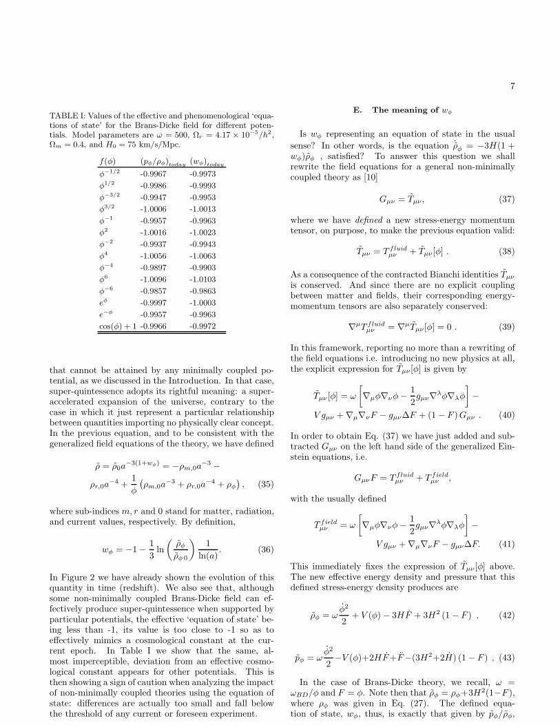
TABLE I: Values of the effective and phenomenological ‘equa-tions of state’ for the Brans-Dicke field for different poten-tials. Model parameters are ω = 500, Ωr = 4.17 × 10−5/h2,Ωm = 0.4, and H0 = 75 km/s/Mpc.

f(φ) (pφ/ρφ)today (wφ)today

φ−1/2 -0.9967 -0.9973

φ1/2 -0.9986 -0.9993

φ−3/2 -0.9947 -0.9953

φ3/2 -1.0006 -1.0013

φ−1 -0.9957 -0.9963

φ2 -1.0016 -1.0023

φ−2 -0.9937 -0.9943

φ4 -1.0056 -1.0063

φ−4 -0.9897 -0.9903

φ6 -1.0096 -1.0103

φ−6 -0.9857 -0.9863

eφ -0.9997 -1.0003

e−φ -0.9957 -0.9963

cos(φ) + 1 -0.9966 -0.9972

that cannot be attained by any minimally coupled po-tential, as we discussed in the Introduction. In that case,super-quintessence adopts its rightful meaning: a super-accelerated expansion of the universe, contrary to thecase in which it just represent a particular relationshipbetween quantities importing no physically clear concept.In the previous equation, and to be consistent with thegeneralized field equations of the theory, we have defined

ρ = ρ0a−3(1+wφ) = −ρm,0a

−3 −

ρr,0a−4 +

1

φ

(

ρm,0a−3 + ρr,0a

−4 + ρφ

)

, (35)

where sub-indices m, r and 0 stand for matter, radiation,and current values, respectively. By definition,

wφ = −1 − 1

3ln

(

ρφ

ρφ 0

)

1

ln(a). (36)

In Figure 2 we have already shown the evolution of thisquantity in time (redshift). We also see that, althoughsome non-minimally coupled Brans-Dicke field can ef-fectively produce super-quintessence when supported byparticular potentials, the effective ‘equation of state’ be-ing less than -1, its value is too close to -1 so as toeffectively mimics a cosmological constant at the cur-rent epoch. In Table I we show that the same, al-most imperceptible, deviation from an effective cosmo-logical constant appears for other potentials. This isthen showing a sign of caution when analyzing the impactof non-minimally coupled theories using the equation ofstate: differences are actually too small and fall belowthe threshold of any current or foreseen experiment.

E. The meaning of wφ

Is wφ representing an equation of state in the usual

sense? In other words, is the equation ˙ρφ = −3H(1 +wφ)ρφ , satisfied? To answer this question we shallrewrite the field equations for a general non-minimallycoupled theory as [10]

Gµν = Tµν , (37)

where we have defined a new stress-energy momentumtensor, on purpose, to make the previous equation valid:

Tµν = T fluidµν + Tµν [φ] . (38)

As a consequence of the contracted Bianchi identities Tµν

is conserved. And since there are no explicit couplingbetween matter and fields, their corresponding energy-momentum tensors are also separately conserved:

∇µT fluidµν = ∇µTµν [φ] = 0 . (39)

In this framework, reporting no more than a rewriting ofthe field equations i.e. introducing no new physics at all,the explicit expression for Tµν [φ] is given by

Tµν [φ] = ω

[

∇µφ∇νφ − 1

2gµν∇λφ∇λφ

]

−

V gµν + ∇µ∇νF − gµν∆F + (1 − F )Gµν . (40)

In order to obtain Eq. (37) we have just added and sub-tracted Gµν on the left hand side of the generalized Ein-stein equations, i.e.

GµνF = T fluidµν + T field

µν ,

with the usually defined

T fieldµν = ω

[

∇µφ∇νφ − 1

2gµν∇λφ∇λφ

]

−

V gµν + ∇µ∇νF − gµν∆F. (41)

This immediately fixes the expression of Tµν [φ] above.The new effective energy density and pressure that thisdefined stress-energy density produces are

ρφ = ωφ2

2+ V (φ) − 3HF + 3H2 (1 − F ) , (42)

pφ = ωφ2

2−V (φ)+2HF +F−(3H2+2H) (1 − F ) , (43)

In the case of Brans-Dicke theory, we recall, ω =ωBD/φ and F = φ. Note then that ρφ = ρφ+3H2(1−F ),where ρφ was given in Eq. (27). The defined equa-tion of state, wφ, thus, is exactly that given by pφ/ρφ,

8

since it was defined using the same Friedmann equationH2 = 1/3(ρfluid + ρφ). Indeed,

ρφ = −ρfluid +1

F(ρfluid + ρφ)

= −ρfluid + 3H2

= −(3H2F − ρφ) + 3H2

= ρφ + 3H2(1 − F ) (44)

At the same time, we can see that

pφ = pφ − (3H2 + 2H) (1 − F ) . (45)

We conclude that the definition for wφ represents a real

equation of state, since it is supported by a conservation

law, and that it is this the one that should be taken into

account to compare with the predictions of GR, since it

is directly related to the observable, H. We can also see,from Table I, that the difference between wφ and theratio pφ/ρφ is very small. The reasons that leads to thisare explicitly discussed for NMC theories in Section III,a similar argument applies here as well.

F. CMB-related observables

The evolution of the comoving distance from the sur-face of last scattering (defined as z = 1000, equivalentlyln a = −6.90) can be computed, for different theories, as:

∫

dτ =

∫ a

0.001

da

a2H(a). (46)

Only in the case of extremely low coupling factors (e.g. ωof Brans-Dicke theory), discarded by current constraints,we see a noticeable difference with the result of GeneralRelativity plus cosmological constant. To give a quanti-tative idea we can quote the ratio

τBD − τGR

τGR

,

calculated today (a = 1), which, for ω = 25 results equalto -0.014, whereas for ω = 500 is −5.7 10−4, and quicklytends to zero for bigger values of ω.

The angular scales at which acoustic oscillations occurare directly proportional to the size of the CMB soundhorizon at decoupling, that in comoving coordinates isroughly τdec/

√3, and inversely proportional to the co-

moving distance covered by CMB photons from last scat-tering until observation, that is τ0 − τdec [34]. The mul-tipoles scale as the inverse of the corresponding angularscale, and so

ℓpeak ∝ τ0 − τdec

τdec

. (47)

As in the non-minimally coupled models studied in Ref.[36], τ changes because of a different dependence of the

Hubble length H−1 in the past. However, we have al-ready noted that this change is almost imperceptiblewhen compared with usual General Relativity plus a cos-mological constant, unless of course (violating currentconstraints) the coupling parameter ω is low enough.

The Integrated Sachs-Wolfe effect makes the CMB co-efficients on large scales, small ℓ’s, change with the varia-tion of the gravitational potential along the CMB photontrajectories [39]. This is undoubtedly changed because ofa variation in the gravitational constant since the timeof decoupling. However, we expect this change to be alsovery small, since the G-variation we have found, for val-ues of ω = 500 and bigger, are typically less than 2%since the time of decoupling.

The scale entering the Hubble horizon at the matter-radiation equivalence is also important, since it will de-fine the matter power turnover [35]. The shift in thepower spectrum turnover is given by [36]

δkturn

kturn

= −(

δH−1

H−1

)

eq

, (48)

and again, this reports a very small difference for all cur-rently possible ω-values. Only for ω = 25 this differenceis about 12% (where a case of a power law potential withexponent equal to -2 taking as an example). For ω = 500and bigger, the differences are less than 1% (to give aprecise example it reports a 0.7% difference in the samepower law case as commented before and ω = 500). Con-trary to what Baccigalupi et al. have done in the past[9] , we are not comparing two different theories (Brans-Dicke and General Relativity) with the same potential,but rather, and motivated by the findings of this section,Brans-Dicke theory with any given potential and GeneralRelativity plus Λ. It is in this case that the possibilitiesof actually distinguishing both situations diminish.

V. NON-MINIMALLY COUPLED THEORIES

The details of the cosmological evolution using the gen-eral action (4) above, with ω = 1 and

F (φ) = 1 + ξφ2 (49)

were explored in Refs. [9, 10, 36], among many others,and we refer the reader to these works and referencestherein for additional relevant discussions. Our nu-merical code is in agreement with the results thereinreported, and it is a direct extension of the numericalimplementation reported in Section IIIB.

In this Section, following the previous discussion, wewould like to focus on the possible definitions of equations

of state and their impact onto observable quantities. Justas an example, we show in Figure 3 the case of a trackingpotential of the form V = V0φ

−2, H0 = 70km/s/Mpc, ina flat universe with Ωm,0 = 0.4. The equivalent Brans-Dicke parameter (obtained by redefining fields in Eq.

9

100

101

102

103

104

105

106

107

108

1E-34

1E-29

1E-24

1E-19

1E-14

log 10

( ρ

[g/c

m3 ] )

1 + z

NMC energy density radiation matter MC energy density

FIG. 3: Matter, radiation and quintessence energy densities,both non-minimally (NMC) and minimally coupled (MC).The incomplete curve corresponds to the non-minimally cou-pled quintessence, and the cutoff is produced by a change inthe sign of the effective density, see text for details.

(4) in order for it to look like a Brans-Dicke theory) isωJBD = ωF/F 2

,φ, and its value is given by defining ξ. Thevalue of ξ used in the model of Figure 3 and successiveones is 5.8 10−3, what implies an equivalent Brans-Dickeparameter ωBD = 3071, well in agreement with currentconstraints.

Starting from the general field equations, we canimmediately define, as done for the Brans-Dicke the-ory, an effective energy density and pressure for thescalar field. The former, for instance, appears writ-ing the 00-component of the field equation as H2 =1/3F (ρfluid + ρφ) . The explicit expression then being,

ρφ =ω

2φ2 + V − 3HF (50)

for the energy density, and

pφ =ω

2φ2 − V + 2HF + F (51)

for the pressure. These two expressions do not, aswe have shown before, pertain to a conserved energy-momentum tensor. They do, however, define an effective

equation of state, this being just pφ/ρφ. This relation-ship is subject to same caveats mentioned above for thecase of Brans-Dicke: it is neither positive nor negativedefined, since the effective energy density itself shifts itssign during the evolution. The energy density quotedabove is what is depicted (whenever possible) in Figure3. As it can be seen, it tracks closely the usually definedminimally coupled (MC) energy density at low redshifts,this being an effect of the necessarily small coupling ξthat is adopted to fulfill observational constraints.

Again, in order to work with a conserved energy-momentum tensor, we can rewrite the field equations andobtain a real equation of state, wφ = pφ/ρφ, where ρφ andpφ were given in Eqs. (42) and (43), respectively. As wealready mentioned in the case of Brans-Dicke, this equa-tion of state is exactly what results in writing the fieldequation as H2 = 1/3(ρfluid + φ), defining implicitlyφ = 1/F (ρfluid + ρφ) − ρfluid. Finally, just for compar-ison, one can as well consider the equation of state forthe case of a minimally coupled scalar field, p/ρ, with

ρ =1

2φ2 + V (φ) , (52)

p =1

2φ2 − V (φ) . (53)

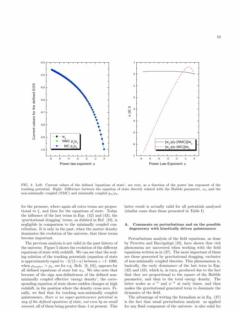
In Figure 4 we show the results of these different def-initions of equation of state for the current time, asa function of the exponent of the power law potentialV = V0 φα, for a flat universe model given by Ωm,0 = 0.4,the same model used in Figure 3. We see that they donot present noticeable differences. Very low values ofthe power law exponent (shallow potentials) are neededto produce equations of state near that generated by acosmological constant. To be quantitative, Figure 4 alsoshows, in the right panel, the differences between theequation of state directly related with the Hubble pa-rameter, wφ and the non-minimally coupled (NMC) andminimally coupled pφ/ρφ. Clearly, the differences are mi-nor. One can actually understand why these differencesare so small. Note that the energy density and pressurein a non-minimally coupled field theory can be written asthe minimally coupled ones plus additional terms. In thecase of ρφ, these terms are equal to −3HF +3H2(1−F ),whereas for ρφ only the first term above enters. Boththese terms are, however, proportional to ξ, being them-selves

−3HF + 3H2(1 − F ) ∼ −6ξHφ − 3ξH2φ2.

But since from the evolution of the field, O(H−1φ)=1 to-day, and at the current era, O(H2) ∼ V , the energy den-

sity can be written as ρφ ∼ ρmc−3ξ( φ2

2 +V φ2), where ρmc

is the minimally coupled energy density. Clearly, at thecurrent cosmological era and because of the constraintson ξ, the second terms are sub-dominant in comparisonto the first ones. A similar analysis can be established

10

-6 -5 -4 -3 -2 -1 0

-1.0

-0.9

-0.8

-0.7

-0.6

-0.5

-0.4

-0.3

wφ

NMC pφ/ρφ

MC pφ/ρφ

Cu

rre

nt

valu

es

for

the

de

fine

d E

OS

Power law exponent: α

-6 -5 -4 -3 -2 -1 0-7

-6

-5

-4

-3

-2

-1

0

1

[wφ-p/ρ (NMC)]/w

φ

[wφ-p/ρ (MC)]/w

φ

x 1

E-3

Power Law Exponent: α

FIG. 4: Left: Current values of the defined ’equations of state’, see text, as a function of the power law exponent of thetracking potential. Right: Difference between the equation of state directly related with the Hubble parameter, wφ and thenon-minimally coupled (NMC) and minimally coupled pφ/ρφ.

for the pressure, where again all extra terms are propor-tional to ξ, and then for the equations of state. Todaythe influence of the last terms in Eqs. (42) and (43), the‘gravitational dragging’ terms, as dubbed in Ref. [10], isnegligible in comparison to the minimally coupled con-tribution. It is only in the past, when the matter densitydominates the evolution of the universe, that these termsbecome important.

The previous analysis is not valid in the past history ofthe universe. Figure 5 shows the evolution of the differentequations of state with redshift. We can see that the scal-ing solution of the tracking potentials (equation of stateis approximately equal to −2/(2+α) between z ∼1–1000,when ρmatter > ρφ, see for e.g. Refs. [9, 10]), appears forall defined equations of state but wφ. We also note thatbecause of the sign non-definiteness of the defined non-minimally coupled effective ‘energy density’, the corre-sponding equation of state shows sudden changes at highredshift, in the position where the density cross zero. Fi-nally, we find that for tracking non-minimally coupledquintessence, there is no super-quintessence potential in

any of the defined equations of state, not even by an small

amount, all of them being greater than -1 at present. This

latter result is actually valid for all potentials analyzed(similar cases than those presented in Table I).

A. Comments on perturbations and on the possible

degeneracy with kinetically driven quintessence

Perturbations analysis of the field equations, as doneby Perrotta and Baccigalupi [10], have shown that richphenomena are uncovered when working with the fieldequations written as in (37). The most important of themare those generated by gravitational dragging, exclusiveof non-minimally coupled theories. This phenomenon is,basically, the early dominance of the last term in Eqs.(42) and (43), which is, in turn, produced due to the factthat they are proportional to the square of the Hubbleparameter, and then to the total energy density. Thelatter scales as a−3 and a−4 at early times, and thenmakes the gravitational generated term to dominate thedynamics of the field.

The advantage of writing the formalism as in Eq. (37)is the fact that usual perturbation analysis –as appliedfor any fluid component of the universe– is also valid for

11

100

101

102

103

104

105

106

107

108

-1.0

-0.5

0.0

0.5

1.0

p/ρ NMC p/ρ MC w

φ

Def

ined

equ

atio

ns o

f sta

te

1 + z

FIG. 5: Evolution in redshift of the equations of state for amodel with V ∝ φ−2.

the field. In that sense, concepts as the equation of state,or the adiabatic sound speed

c2φ =

˙pφ

˙ρφ

= wφ − 1

3H

wφ

1 + wφ

, (54)

(where we have made use of the field conservation equa-tion) can be well defined. If the field is slowly varyingin time, c2

φ ∼ wφ. Hu [39] showed, for negative equa-tions of state, that adiabatic fluctuations are unable togive support against gravitational collapse. Density per-turbations would become non-linear after entering thehorizon, unless the entropic term wφΓφ > 0 [39].

The effective sound speed, c2eff ,φ, is then defined in the

rest frame of the scalar field, where δT 0j φ = 0 [39]. The

gauge invariant entropic term is written as wφΓφ = (c2eff−

c2φ)δ

(rest)φ , where δ

(rest)φ is the density contrast in the dark

energy rest frame [10] δ(rest)φ = δφ+3H

k(1 + wφ) (vφ − B)

(we refer the reader to Ref. [10] for more careful expla-nations). For normal quintessence, the effective soundspeed is c2

eff ,φ = 1, giving a relativistic behavior to thecorresponding density fluctuations. However, Perrottaand Baccigalupi [10] have found that the situation can

be much different for non-minimally coupled gravity. Inthat case,

c2eff ,φ ∼ δpφ

δρφ

(55)

for values of k ≫ H . But because of gravitational drag-ging, δρφ can be quite difference from the usual case, andthis ratio may be much lower than unity whenever theenergy density perturbations of the scalar field are en-hanced by perturbations in the matter field. At the levelof perturbations, then, quite distinctive effects appearsin non-minimally coupled quintessence as compared withthe usual case and make these theories possibly distin-guishable.

Very recently, yet another scenario for an alternativemodel of quintessence was introduced [37]. In it, knownas k-essence, the Lagrangian density includes a non-canonic kinetic term:

S =

∫

d4x√−g

(

1

16πGR + p(φ,∇φ)

)

+ Sm,r, (56)

where Sm,r denotes the action for matter and/or ra-diation. Examples in which the Lagrangian dependsonly on the scalar field φ and its derivative squaredX = − 1

2∇µφ∇µφ. have been constructed [37]. The fieldequations for this models are

Rµν − 1

2gµνR =

8πG

(

∂p(φ, X)

∂X∇µφ∇νφ + p(φ, X)gµν + T m,r

µν

)

(57)

where T m,rµν is the energy-momentum tensor for usual

matter fields. p(φ, X) corresponds to the pressure ofthe scalar field, whereas the energy density is given byρφ = 2X∂p/∂X − p [38]. It can be seen that for thismodels, the speed of sound is given by [40]

c2eff =

pQ,X

ρQ,X

=p,X

p,X + 2Xp,XX

. (58)

Apparently, then, and since p is completely generic, itcould exist a non-canonic kinetic term within k-essencegiving rise to the same results of non-minimally coupledgravity. Viscosity (a parameter relating velocity and met-ric shear with anisotropic stress [39]) can however pro-vide the way to break the degeneracy, since it resultsnon-zero for a non-minimally coupled field (contrary aswell to what results in usual quintessence) [10].

VI. CONCLUSIONS

In the case of Brans-Dicke theory, and in the casesof ωBD allowed by current constraints, we have numer-ically proven that the homogeneous field equations ofextended quintessence yield to no observable effect that

12

can distinguish the theory from the predictions of Gen-eral Relativity plus a cosmological constant. It is withthis model that the comparison should be made, sincefor the large values of the coupling parameters requiredby current experiments, all potentials are closely similarto a constant function, and the theory itself to GeneralRelativity. Although we have not made a detailed per-turbation analysis using the full numerical CMBFASTcode, we can safely predict that the same situation willhappen there, as a result of the analysis made for theCMB-related observables in Section IIC. We discussedthe observationally-related definition of equation of statewφ, and not to the usually studied ratio between the ef-fective pressure and density directly obtained from thefield equations, to which we assign no particular physi-cal meaning. The phenomenon of super-quintessence, i.e.a super-accelerated expansion of the universe, althoughpossible for a non-minimally coupled Brans-Dicke scalarfield, and impossible in any minimally coupled field situ-ation, it is of such an small amount that is far beyond theexpectations of any realistic experiment. From a practi-cal point of view, then, it will always exist a scalar fieldpotential supporting a minimally coupled field that pro-duces experimentally indistinguishable results from thoseobtained within the extended quintessence framework ofBrans-Dicke theory.

For the more general extended non-minimally cou-pled models studied, the possibility of having super-quintessence actually disappears: all tracking potentialsexplored produce effective equations of state greater than-1. We have shown that for low values of the exponentin the tracking potentials supporting the non-minimallycoupled field (i.e. equations of state are close to -1), thedifference among all defined equations of state is negli-gible. It is, however, in the perturbation regime wheredifferences with the usual quintessence case can be no-ticed. As Perrotta and Baccigalupi have found [10], a newgravitational dragging effect appears here, giving rise tothe possibility of clumps of scalar field matter. In thiscase, however, it is with k-essence models that a degen-eracy could appear, particularly in those cases in whichp,X +2Xp,XX ≫ 1, yielding the speed of sound to valuesclose to zero.

Finally, we remark that expanding solutions whereacceleration is transient have been recently consideredgiven the consistency problem between string theory andspaces with future horizons [43]. Since scalar-tensor theo-ries of gravity likely originate in string theory, it would beinteresting to make a similar analysis to that presentedin the previous reference for the case of non-minimallycoupled theories.

Acknowledgments

It is a pleasure to warmly acknowledge Prof. Uros Sel-jak. His contribution and permanent advice were invalu-able. Very useful discussions with Dr. F. Perrotta, as

well as interesting comments by Dr. A. Mazumdar, arealso thankfully acknowledged. Dr. Perrotta is furtheracknowledged for his critical reading of the manuscript.An important improvement of the paper has been possi-ble after useful remarks from an anonymous Referee.

Appendix

In the literature, one may find two alternative in-troductions of general non-minimally coupled theories.Firstly, the one that we follow in Section II (see for in-stance [42]), and secondly, the one that is derived fromthe action

S =

∫

d4x√−g

[

1

2κf(φ, R) − ω(φ)

2∇µφ∇µφ

−V (φ) + Lfluid] , (59)

where κ is a constant, not necessarily taken as 1, andplays the role of the “bare” gravitational constant (seefor instance [12], by the same authors). The function fis then assumed to be of the form

(1/κ)f(φ, R) = F (φ)R. (60)

The function F , in the case we are interested in, is writtenas

F (φ) =1

κ+ ξφ2 = 1 + ξ(φ2 − φ2

0). (61)

Then, a value of κ = 1, as we have taken in the theoret-ical development of the previous sections just reduces totake φ0, the current value of the field, equal to 0. This,however, is not what may result, in general, numericallyconvenient, since it would imply to precisely fix the evo-lution of the field to reach φ = 0 today. Instead, as weare not actually interested in any value of κ per se, we donot make κ = 1 in our numerical code, and instead followthe treatment given by Perrotta and Baccigalupi ([10]).In that case, they choose to rewrite the field equations as

Gµν = κTµν , (62)

with the corresponding field energy density and pressuregiven by

ρφ = ωφ2

2+ V (φ) − 3HF + 3H2

(

1

κ− F

)

, (63)

pφ = ωφ2

2− V (φ) + 2HF + F − (3H2 + 2H)

(

1

κ− F

)

.

(64)When comparing Eq. (62) with the usual Einstein equa-tions, one has to take into account that the value of κ isnot 1 (although certainly it is truly close to unity, becauseof the constraint imposed on ξ). Then, if we decide towrite the Friedman equation like H2 = 1/3(ρfluid + φ),

13

to directly compare with GR (and the same matter den-sity) the corresponding relationship between φ and ρφ

give in Eq. (63) is

φ = (κ − 1)ρfluid + κρφ. (65)

In this scheme, pφ/ρφ (with quantities defined as in Eqs.(63) and (64)) will differ from the equation

wφ = −1 − 1

3ln

(

φ

φ 0

)

1

ln(a), (66)

because φ 6= ρφ, but it is the latter Eq. (66) what shouldbe used to compare with the results of General Relativitywith a fixed current matter density.

[1] A. Riess et al. Astron. J 116, 1009 (1998); S Perlmutteret al. ApJ 517 565 (1999).

[2] See, for example, P. De Bernardis et al., ApJ, 564, 559(2002).

[3] P. J. Peebles, B. Ratra, Astrophys. J. 352, L17 (1988);R.R. Caldwell, R. Dave, P. J. Steinhardt, Phys. Rev.Lett. 80, 1582 (1998).

[4] V. Sahni, and A. Starobinsky, Int.J.Mod.Phys. D9,373(2000).

[5] L. Wang, R. R. Caldwell, J. P. Ostriker, P. J. Steinhardt,ApJ 530, 17 (2000); P.J. Steinhardt, L. Wang, I. Zlatev,Phys. Rev. D59, 123504 (1999); I. Zlatev, L. Wang, P.J.Steinhardt, Phys. Rev. Lett. 82, 896 (1999); A.R. Liddle,R.J. Scherrer, Phys. Rev. D59, 023509 (1999).

[6] V. Faraoni, astro-ph/0110067 (2001); E. Gunzig, A.Saa, L. Brenig, V. Faraoni, T.M. Rocha Filho and A.Figueiredo, Phys. Rev. D63 067301, (2001).

[7] R. R. Caldwell, astro-ph/9908168[8] S. Sen and T. R. Seshadri, To be published in Int. J.

Mod. Phys. D, gr-qc/0007079[9] F. Perrotta, C. Baccigalupi, and S. Matarrese, Phys. Rev.

D61, 023507 (1999).[10] F. Perrotta, and C. Baccigalupi, astro-ph/0201335[11] J. P. Uzan, Phys.Rev. D59, 123510 (1999); A. Riazuelo

and J. P. Uzan, astro-ph/0107386[12] G. Esposito-Farese, and D. Polarski, Phys. Rev. D63,

063504 (2001).[13] T. Chiba, Phys. Rev. D64, 103503 (2001).[14] L. Amendola, Phys. Rev. D60, 043501 (1999); O. Berto-

lami and P. Martins, Phys. Rev. D61, 064007 (2000); D.Holden and D. Wands, Phys. Rev. D61, 043506 (2000);Y. Fujii, Phys. Rev. D62, 044011 (2000); F. Perrotta andC. Baccigalupi astro-ph/0205245; S. Capozziello, Int. J.Mod. Phys. D11, 483 (2002).

[15] C. Santos, and R. Gregory, Annals Phys. 258, 111 (1997).[16] M. Visser, Lorentzian Wormholes (AIP, New York, 1996).[17] C. Barcelo and M. Visser, Phys. Lett. B466, 127 (1999);

C. Barcelo and M. Visser, Class. Quant. Grav. 17, 3843(2000).

[18] J. Cramer, R. Forward, M. Morris, M. Visser, G. Ben-ford, and G. Landis, Phys. Rev. D 51, 3117 (1995);D. F. Torres, E. F. Eiroa and G. E. Romero, Mod. Phys.Lett. A 16, 1849 (2001); M. Safonova, D. F. Torres andG. E. Romero, Phys. Rev. D 65, 023001 (2002); E. Eiroa,G. E. Romero and D. F. Torres, Mod. Phys. Lett. A 16,973 (2001); M. Safonova, D. F. Torres and G. E. Romero,Mod. Phys. Lett. A 16, 153 (2001); L. A. Anchor-doqui, S. Capozziello, G. Lambiase and D. F. Torres,

Mod. Phys. Lett. A 15, 2219 (2000); L. A. Anchordoqui,G. E. Romero, D. F. Torres and I. Andruchow, Mod.Phys. Lett. A 14, 791 (1999); G. E. Romero, D. F. Tor-res, I. Andruchow, L. A. Anchordoqui and B. Link, Mon.Not. Roy. Astron. Soc. 308, 799 (1999); D. F. Torres,G. E. Romero and L. A. Anchordoqui, Mod. Phys. Lett.A 13, 1575 (1998); ibid. Phys. Rev. D 58, 123001 (1998).

[19] A. DeBenedictis and A. Das [gr-qc/0009072]; S. E. PerezBergliaffa and K. E. Hibberd, Phys. Rev. D 62, 044045(2000); C. Barcelo and M. Visser, Nucl. Phys. B584,415 (2000); L. A. Anchordoqui and S. E. Perez Bergliaffa,Phys. Rev. D 62, 067502 (2000); D. Hochberg, A. Popov,and S. V. Sushkov, Phys. Rev. Lett. 78, 2050 (1997); S.Kim and H. Lee, Phys. Lett. B 458, 245 (1999); S. Kras-nikov, Phys. Rev. D 62, 084028 (2000); D. Hochberg andM. Visser, Phys. Rev. D 56, 4745 (1997); L. A. Anchor-doqui, S. Perez Bergliaffa and D. F. Torres, Phys. Rev.D 55, 5226 (1997); L. A. Anchordoqui, D. F. Torres,M. L. Trobo and S. E. Perez Bergliaffa, Phys. Rev. D 57,829 (1998).

[20] M. Visser, Phys. Rev. D 56, 7578 (1997); Science 276,88 (1997).

[21] A. R. Liddle and D. H. Lyth, Cosmological inflation and

large scale structure, (Cambridge University Press, Cam-bridge, 2000, pp. 20).

[22] R. D. Reasenberg et al., Astrophys.J. 234, L219 (1979).[23] See C. Will, gr-qc/0103036[24] C. M. Will, Theory and Experiment in Gravitational

Physics, (Cambridge University Press, Cambridge, Eng-land, 1993).

[25] B. M. Barker, ApJ 219, 5 (1978).[26] F. S. Accetta, L. M. Krauss and P. Romanelli, Phys.

Lett. B248, 146 (1990); D. F. Torres, Phys. Lett. B 359,249 (1995); J. A. Casas, J. Garcıa-Bellido and M. Quiros,Mod. Phys. Lett. A7, 447 (1992), Phys. Lett. B278, 94(1992); D. I. Santiago, D. Kalligas, R. V. Wagoner, Phys.Rev. D56, 7627 (1997); A. Serna, R. Domingues-Tenreiroand G. Yepes, ApJ 391, 433 (1992).

[27] J. P. Mimoso, and D. Wands, Phys. Rev. D52, 5612(1995).

[28] J. D. Barrow, and J. P. Mimoso, Phys. Rev. D50, 3746(1994); J. D. Barrow, and P. Parsons, Phys. Rev. D55,1906 (1997).

[29] D. F. Torres and H. Vucetich, Phys. Rev. D 54, 7373(1996); D. F. Torres, Phys. Lett. A 225, 13 (1997).

[30] C. Brans and R. H. Dicke, Phys. Rev. 124, 925 (1961).[31] A. R. Liddle, A. Mazumdar, and J. D. Barrow, Phys.

Rev. D58, 027302 (1998).

14

[32] D. I. Santiago, and A. S. Silbergleit Gen. Rel. Grav. 32,565 (2000).

[33] S. Weinberg, Gravitation and cosmology (Wiley, NewYork, 1972).

[34] W. Hu, U. Seljak, M. White, M. Zaldarriaga, Phys. Rev.D57, 3290 (1998).

[35] K. Coble, S. Dodelson, and J. Friemann, Phys. Rev. D55,1851 (1997).

[36] C. Baccigalupi, S. Matarrese, and F. Perrotta, Phys. Rev.D62, 123510 (1999).

[37] T. Chiba, T. Okabe, and M. Yamaguchi, Phys. Rev.Phys. Rev. D62, 023511 (2000), C. Armendariz-Picon,V. Mukhanov, and P. J. Steinhardt, Phys. Rev. Lett. 85,4438 (2000), ibid. Phys. Rev. D63, 103510 (2000).

[38] C. Armendariz-Picon, T. Damour, and V. Mukhanov,

Phys. Lett. B458, 209 (1999).[39] W. Hu, ApJ 506, 485 (1998).[40] J. K. Erickson, R. R. Caldwell, Paul J. Steinhardt, C.

Armendariz-Picon, and V. Mukhanov, astro-ph/0112438[41] N. Banerjee and S. Sen, Phys. Rev. D56, 1334 (1997).[42] B. Boisseau, G. Esposito-Farese, D. Polarski, and A. A.

Starobinsky, Phys. Rev. Lett. 85, 2236 (2000).[43] S. Hellerman, N. Kaloper, L. Susskind, JHEP 0106, 003

(2001).[44] Strictly speaking, this seems to be true only in the cases

in which the trace of the energy-momentum tensor fornormal matter fields is not zero (see [41] and referencestherein).