Measuring complete quantum states with a single observable

Xinhua Peng1,∗ Jiangfeng Du1,2, and Dieter Suter1

1Fachbereich Physik, Universitat Dortmund, 44221 Dortmund, Germany and2Hefei National Laboratory for Physical Sciences at Microscale and Department of Modern Physics,

University of Science and Technology of China, Hefei, Anhui 230026, P.R. China(Dated: March 24, 2008)

Experimental determination of an unknown quantum state usually requires several incompatiblemeasurements. However, it is also possible to determine the full quantum state from a single, re-peated measurement. For this purpose, the quantum system whose state is to be determined is firstcoupled to a second quantum system (the “assistant”) in such a way that part of the information inthe quantum state is transferred to the assistant. The actual measurement is then performed on theenlarged system including the original system and the assistant. We discuss in detail the require-ments of this procedure and experimentally implement it on a simple quantum system consisting ofnuclear spins.

PACS numbers: 03.65.Wj, 03.67.-a, 05.30.-d

I. INTRODUCTION

Given the state of a quantum system, one is able tocalculate the results of any measurement performed onthat system. However, to determine the state from theresults of measurements, one usually has to perform dif-ferent measurements that are not mutually compatible,using non-commuting observables. This issue is some-times referred to as the ”Pauli problem”, since Pauli dis-cussed it in 1933 [1] Since then, interest in this issue hascontinued, as it touches the fundamentals of quantummechanics [2] More recently, it was also found to be ofpractical importance in quantum communication [3, 4, 5], e.g., in quantum cryptography and quantum key distri-bution [6, 7].

If we consider an ensemble S of N -level systems, itsquantum state is described by a density matrix ρ in N -dimensional Hilbert space, which requires N2 − 1 realparameters for its complete specification. These parame-ters can be determined experimentally from the outcomesof a series of different measurements on identically pre-pared ensembles. Since quantum mechanical measure-ments with an observable Ω with the spectral decompo-sition Ω =

∑Nα=1$αPα generate at most N − 1 indepen-

dent probabilities, at least (N2−1)/(N−1) = N+1 mea-surements with noncommuting observables are requiredto fully determine the unknown state ρ.

Techniques for the reconstruction of the completequantum state from a series of measurements are com-monly referred to as “quantum state tomography” [8, 9,10]. Different versions of such techniques have been pro-posed, with the goal of obtaining the best possible infor-mation about the unknown state while using the smallestpossible number of measurements. Since the number ofmeasurements must be at least N + 1, the task is thusto determine an optimal set of N + 1 observables (see,

∗Electronic address: xinhua@e3.physik.uni-dortmund.de

e.g.,[11]). A solution to this problem was given by Woot-ters and Fields [12]: They found that the observablesshould be chosen such that their basis states are evenlydistributed through Hilbert space “mutually unbiased”).This choice assures that the data redundancy is mini-mized and the information content is maximized.

As the simplest example, we consider the state of aspin 1/2. Its density operator can be written in the formρ = 1

2 (1 + ~s · ~σ), where ~σ are the Pauli operators and ~sis a dimensionless vector of length ≤ 1 that specifies theposition of the state in the Bloch sphere.

The simplest approach to determine this state consistsof measuring the spin components along the x, y, and z-axes, yielding 6 possible measurement outcomes (see Fig.1 a). A minimal set of measurements only requires foursuch probabilities. They may be chosen as the proba-bilities for measuring the spin operator components infour directions that are oriented like the face normals ofa tetrahedron [13].

While these approaches all require a combination ofmeasurements with incompatible observables, it is alsopossible to obtain the complete state information from asingle measurement performed on a larger Hilbert space,provided the state information is first redistributed intothis extended space [14, 15, 16, 17]. Ref. [14] shows thatit is possible to estimate the expectation values of all ob-servables of a quantum system by measuring only a single“universal” observable on an extended Hilbert space. Inthe Hilbert space of the quantum system, the reduced op-erator of this “universal observable” constitutes a min-imal informationally complete positive operator-valuedmeasurement [15]. Du et al. [16] demonstrated an ex-perimental example on this. Allahverdyan et al. [17]determine the conditions for making this type of mea-surement robust by maximizing the determinant of themapping between the quantum state and the measure-ment results.

The possibility of obtaining the full quantum state in-formation from a single measurement appears highly at-tractive and may well have practical advantages since it

arX

iv:0

803.

3398

v1 [

quan

t-ph

] 2

4 M

ar 2

008

2

a) b)

y

x

zPz Py

Px Pθ

SS

A

θ

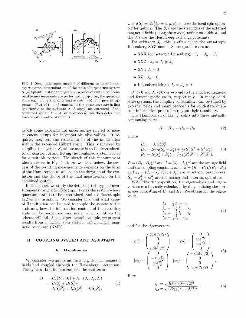
FIG. 1: Schematic representation of different schemes for theexperimental determination of the state of a quantum systemS. (a) Quantum state tomography: a series of mutually incom-patible measurements are performed, projecting the quantumstate e.g. along the x, y, and z-axes. (b) The present ap-proach: Part of the information in the quantum state is firsttransferred to the assistant A. A single measurement of thecombined system S + A, in direction θ, can then determinethe complete initial state of S.

avoids some experimental uncertainties related to mea-surement setups for incompatible observables. It re-quires, however, the redistribution of the informationwithin the extended Hilbert space. This is achieved bycoupling the system S, whose state is to be determined,to an assistant A and letting the combined system evolvefor a suitable period. The sketch of this measurementidea is shown in Fig. 1 b). As we show below, the suc-cess of the resulting measurements depends on the formof the Hamiltonian as well as on the duration of the evo-lution and the choice of the final measurement on thecombined system.

In this paper, we study the details of this type of mea-surements using a (nuclear) spin 1/2 as the system whosequantum state is to be determined, and a different spin1/2 as the assistant. We consider in detail what typesof Hamiltonian can be used to couple the system to theassistant, how the information content of the resultingstate can be maximized, and under what conditions thescheme will fail. As an experimental example, we presentresults from a nuclear spin system, using nuclear mag-netic resonance (NMR).

II. COUPLING SYSTEM AND ASSISTANT

A. Hamiltonian

We consider two qubits interacting with local magneticfields and coupled through the Heisenberg interaction.The system Hamiltonian can then be written as

H = Hz(B1, B2) + Hex(Jx, Jy, Jz)= B1S

1z +B2S

2z+

JxS1xS

2x + JyS

1y S

2y + JzS

1z S

2z ,

(1)

where Skν = 12σ

kν (ν = x, y, z) denotes the local spin opera-

tor for qubit k. The Bks are the strengths of the externalmagnetic fields (along the z axis) acting on qubit k, andthe Jνs are the Heisenberg exchange constants.

For arbitrary Jν , this is often called the anisotropicHeisenberg XYZ model. Some special cases are:

• XXX (or isotropic Heisenberg): Jx = Jy = Jz

• XXZ : Jx = Jy 6= Jz

• XY : Jz = 0

• XZ : Jy = 0

• Heisenberg-Ising : Jx = Jy = 0

Jν > 0 and Jν < 0 correspond to the antiferromagneticand ferromagnetic cases, respectively. In many solid-state systems, the coupling constants Jν can be tuned byexternal fields and many proposals for solid-state quan-tum information processors rely on their tunability.

The Hamiltonian of Eq (1) splits into three mutuallycommuting parts,

H = Hzz + H0 + H2 (2)

where

Hzz = JzS1z S

2z

H0 = BγB(S1z − S2

z ) + J2 (S1

+S2− + S1

−S2+)

H2 = B(S1z + S2

z ) + J2 γJ(S1

+S2+ + S1

−S2−).

(3)

B = (B1+B2)/2 and J = (Jx+Jy)/2 are the average fieldand the coupling constant, and γB = (B1−B2)/(B1+B2)and γJ = (Jx−Jy)/(Jx+Jy) are anisotropy parameters.Sk± = Skx + iSky are the raising and lowering operators.

With this decomposition, the eigenvalues and eigen-vectors can be easily calculated by diagonalizing the sub-spaces consisting of H0 and H2. We obtain for the eigen-values

λ1 = 14Jz + η1,

λ2 = − 14Jz + η2,

λ3 = − 14Jz − η2,

λ4 = 14Jz − η1,

(4)

and for the eigenvectors

|ψ1〉 =

cos(θ1/2)00

sin(θ1/2)

|ψ2〉 =

0

cos θ22sin θ2

20

|ψ3〉 =

0

− sin θ22

cos θ220

|ψ4〉 =

− sin(θ1/2)00

cos(θ1/2)

.

(5)

Here

η1 =√B2 + (JγJ/2)2

η2 =√

(BγB)2 + (J/2)2. (6)

3

and

cos θ12 =√

η1+B2η1

sin θ12 = JγJ/2√

2η1(η1+B)= sgn(JγJ)

√η1−B2η1

cos θ22 =√

η2+BγB2η2

sin θ22 = J/2√

2η2(η2+BγB)= sgn(J)

√η2−BγB

2η2

. (7)

B. Evolution

We write the evolution operator as a product of theevolutions generated by the three mutually commutingterms of Eq. (2):

U(τ) = e−iHτ = Uzz(τ)U0(τ)U2(τ) (8)

where

Uzz(τ) = e−iHzzτ

= cos(Jzτ4 )1− i sin(Jzτ4 )(4S1z S

2z )

U0(τ) = e−iH0τ

= 1+cos(η2τ)2 1 + 1−cos(η2τ)

2 (4S1z S

2z )+

i2 cos θ2 sin(η2τ)(S1z − S2

z )+i sin θ2 sin(η2τ)(S1

+S2− + S1

−S2+)

U2(τ) = e−iH2τ

= 1+cos(η1τ)2 1− 1−cos(η1τ)

2 (4S1z S

2z )+

i2 cos θ1 sin(η1τ)(S1z + S2

z )+i sin θ1 sin(η1τ)(S1

+S2+ + S1

−S2−).

(9)

In the following, we will use a different operator basisfor the diagonal terms: we define the polarization oper-ators Iα,βi = 1

21 ± S(i)z . In terms of these operators, the

total propagator becomes

U(τ) = a1Iα1 I

α2 + a2I

α1 I

β2 + a3I

β1 I

α2 + a4I

β1 I

β2

+d(S1+S

2− + S1

−S2+) + b(S1

+S2+ + S1

−S2−), (10)

where

a1 = cos2 θ12 e−iλ1τ + sin2 θ1

2 e−iλ4τ

a2 = cos2 θ22 e−iλ2τ + sin2 θ2

2 e−iλ3τ

a3 = sin2 θ22 e−iλ2τ + cos2 θ2

2 e−iλ3τ

a4 = sin2 θ12 e−iλ1τ + cos2 θ1

2 e−iλ4τ

b = 12 sin θ1(e−iλ1τ − e−iλ4τ )

d = 12 sin θ2(e−iλ2τ − e−iλ3τ ).

(11)

As we show in the following section, the evolution ofEq. (8) transfers information between qubits in such away that it becomes possible to measure the completequantum state of one qubit with a single apparatus, asproposed by Allahverdyan et al.[17].

III. MEASUREMENT PROCEDURE

A. Principle

Consider a two-level system S (spin- 12 ) whose state can

be represented by ρ =(ρ11 ρ12

ρ21 ρ22

)with the normaliza-

tion ρ11 + ρ22 = 1. To determine the state ρ, we can

measure the vector ~s = 2Tr( ~Sρ) = (sx, sy, sz)T wheresx = ρ12 + ρ21, sy = i(ρ12 − ρ21), sz = ρ11 − ρ22 and~S = (Sx, Sy, Sz)T .

To transfer part of the state information to the assis-tant A, we couple the two subsystems with the interac-tion Hamiltonian H of Eq.(1). At the time t = 0, thecomposite system S+A is in the state %0 = ρ(S) ⊗ ξ(A).Without loss of generality, we assume ξ = 1

21+ εSz, (0 ≤ε ≤ 1). Here, the superscripts S and A refer to the twosubsystems.

Under the effect of the coupling Hamiltonian of Eq.(1), this state evolves into %τ = U(τ) %0 U

†(τ). Onthis state, we perform repeatedly measure the sim-plest possible nondegenerate, factorized observable Ω =∑4α=1$αPα, which determines the complete set Pα of

the joint probabilities, They correspond to the eigenval-ues of %τ in the eigenbasis of the observable Ω. Sincethese values were generated from the initial state by aone-to-one mapping, Pα = Pkq =

∑ijMkq,ijρij , we can

invert this mapping to calculate the original state ρ [17].The precision of the back-calculation depends on the

size of the determinant ∆ = det(Mkq,ij): If |∆| is small,any (experimental) error in the measurement of Pkq willresult in a large error in ρij , roughly ∝ 1/|∆|. We there-fore seek to maximize |∆| and thereby the precision ofthe measurement. This maximization is achieved by asuitable choice of the Hamiltonian H, the duration τ ,and the single observable Ω.

B. Symmetry properties of the evolution

The Hamiltonian H of Eq. (1) consists of three com-muting parts: Hzz, H0, and H2. All of these terms areinvariant under π-rotations around the z-axis. We usethis property to separate the density operator into twoparts that transform irreducibly under this symmetry op-eration: One part which is invariant with respect to πzrotations, and the second part, which changes sign. Thefirst part includes diagonal terms, zero quantum and dou-ble quantum coherence [18]; the second part includes thesingle quantum coherence terms. The symmetry of theHamiltonian implies that the evolution does not transferinformation from one subspace to the other. Figure 2illustrates the division of the density operator into thesesubspaces.

A consequence of this separation of the system into twodistinct subspaces is that it restricts the possible choice of

4

SQCSQC

SQC

SQC

ZQC&DQC

FIG. 2: Subspaces of the density operator that are invariantby the evolution under the Hamiltonian of Eq. (1).

observables. In particular, if we choose the z-componentsof the two spins to the single observable Ω, then all pos-sible combinations fall into the subspace that is invariantunder πz rotations and therefore does not provide infor-mation about the other subspace. For this paper, wechoose the x-components of both spins; another, equiva-lent choice would be the y-components.

C. Transfer matrix

This evolution process, together with the subsequentmeasurement of the single observable Ω, transfers theinformation from the initial state %0 to the set of mea-surement results Pα = Pkq, which are the expectationvalues of the operators

Pkq = (121− (−1)kS(S)

x )⊗ (121− (−1)qS(A)

x )

acting on the state %τ :

Pkq = TrPkqU(τ)%0U†(τ).

The indices k, q can have the values 1, 2.We use the transfer matrix M to describe this map:

M

ρ11

ρ12

ρ21

ρ22

=

P11

P12

P21

P22

. (12)

Its elements are

M11,11 =M22,11 = 18 ((1 + ε)|a1 + b|2 + (1− ε)|a2 + d|2)

M12,11 =M21,11 = 18 ((1 + ε)|a1 − b|2 + (1− ε)|a2 − d|2)

M11,12 = −M22,12 =M∗11,21 = −M∗22,21

= 18 ((1 + ε)(a1 + b)(a∗3 + d∗) + (1− ε)(a2 + d)(a∗4 + b∗)

M22,22 = −M21,12 =M∗12,21 = −M∗33

= 18 ((1 + ε)(a1 − b)(a∗3 − d∗) + (1− ε)(a2 − d)(a∗4 − b∗)

M11,22 =M22,22 = 18 ((1 + ε)|a3 + d|2 + (1− ε)|a4 + b|2)

M12,22 =M21,22 = 18 ((1 + ε)|a3 − d|2 + (1− ε)|a4 − b|2)

(13)

and its determinant is

∆ = 8=(M∗12,12M11,12)(M11,11M12,22−M12,11M11,22).(14)

Here =(c) denotes the imaginary part of c. Using Eqs.(4), (7), (11) and (13), we find for its absolute value

|∆| = 132 |(1− ε

2) sin(−Jzτ)[sin(2θ1) sin2(η1τ)]2−[sin(2θ2) sin2(η2τ)]2+ 2ε[sin(2θ1) sin2(η1τ)+ sin(2θ2) sin2(η2τ)][1− 2 sin2 θ1 sin2(η1τ)]× sin θ2 sin(2η2τ)− [1− 2 sin2 θ2 sin2(η2τ)]× sin θ1 sin(2η1τ)|.

(15)

IV. OPTIMIZATION: MAXIMIZING |∆|

The size of the determinant |∆| of the transfer map-ping determines the quality of measurement. Maximizing|∆| will minimize the statistical error of the estimationduring the inversion of Eq. (12). We can maximize it byan appropriate choice of the initial condition of the assis-tant, the parameters of the Hamiltonian that generatesthe evolution U , and the duration of the evolution.

Figure 3 plots the maximum possible determinant size|∆|max for the Hamiltonian of Eq. (1) as a function ofthe polarization ε of the assistant. Clearly, the quality ofthe measurement should increase with increasing polar-ization of the assistant. The dashed line in Fig. 3 showsfor comparison the maximum possible value for a gen-eral exchange interaction, taken from Ref. [17]. At theextreme cases of zero and full polarization, the Heisen-berg coupling Hamiltonian allows one to reach the max-imum possible value, but for intermediate polarizations,its maximum value is slightly lower than for the generalcase.

Let us now focus on two extreme situations ε = 1 (apure state) and ε = 0 (a completely disordered state).

0 0.2 0.4 0.6 0.8 10.03

0.04

0.05

ε

|∆| m

ax

Our resultEq.(9) in Ref. [17]

1/32

1/(12 × 31/2)

FIG. 3: (Color Online) Maximal determinant size |∆|max ver-sus the polarization ε by the Heisenberg exchange interaction(1), compared to the general case of arbitrary exchange inter-action (Eq. (9)) in Ref. [17]).

5

A. Assistant in pure state

When the assistant A starts in a pure state ξ(A) =121 + S

(A)z (corresponding to ε = 1), the determinant

becomes

|∆| = 116 |[sin(2θ1) sin2(η1τ) + sin(2θ2) sin2(η2τ)]×[1− 2 sin2 θ1 sin2(η1τ)] sin θ2 sin(2η2τ)−[1− 2 sin2 θ2 sin2(η2τ)] sin θ1 sin(2η1τ)|.

(16)We can see from this expression that |∆| is independent ofthe coupling strength Jz along the z-axis. A HeisenbergXY interaction is therefore sufficient for optimizing theevolution. We therefore specialize to this case. Using thesubstitutions

sin Ξk2 = sin θk sin(ηkτ)

sin Λk = cos(ηkτ)/ cos Ξk2 , (k = 1, 2),

(17)

we rewrite |∆| as

|∆| = 116 |(sin Ξ1 cos Λ1 + sin Ξ2 cos Λ2)×(cos Ξ1 sin Ξ2 sin Λ2 − cos Ξ2 sin Ξ1 sin Λ1)|.

(18)In terms of these parameters, an optimal solution (|∆| =1/(12

√3)) is given by the following set of parameters:

Λ1 = Λ2 = Λsin(2Λ) = ±1sin Ξ1−Ξ2

2 = ± 1√3

sin Ξ1+Ξ22 = ±1.

(19)

This parameter set corresponds to the following param-eters of the Hamiltonian (1):

ηkτ = mπ ± 12 arccos(−Γk)

B = ±η1

√(1− Γ1)/(1 + Γ1)

γB = ±√

(1+Γ1)(1−Γ2)(1−Γ1)(1+Γ2)

η2η1

J = ±4η2

√2Γ2/(1 + Γ2)

γJ = ±√

Γ1(1+Γ2)Γ2(1+Γ1)

η1η2.

(20)

Here, m is an integer and Γk = sin2 Ξk2 , (k = 1, 2).

(Γ1,Γ2) take the pairs of values ( 12 −

√3

6 ,12 +

√3

6 ) or( 1

2 +√

36 ,

12 −

√3

6 ). Without loss of generality, we setτ = 1. The optimal Hamiltonian is then

Hopt = 1.1458S1z −0.2935S2

z +3.3820S1xS

2x−1.2747S1

y S2y .

(21)

B. Completely disordered assistant.

When the assistant A is initially in a completely dis-ordered state ξ(A) = 1

21 (ε = 0), we have

|∆| = 132 | sin(−Jzτ)||[(sin(2θ1) sin2(η1τ)]2

−[(sin(2θ2) sin2(η2τ)]2|. (22)

|∆| reaches its maximum of 1/32 when

sin(Jzτ) = ±1⇒ Jzτ =π

2(2n− 1) (23)

(n integer) and simultaneously

sin(2θ1) sin2(η1τ) = ±1 and sin(2θ2) sin2(η2τ) = 0(24)

or

sin(2θ1) sin2(η1τ) = 0 and sin(2θ2) sin2(η2τ) = ±1.(25)

Condition (24) corresponds to the following parame-ters for the Hamiltonian:

|B|τ = |2m− 1|√

2π4

|Jx − Jy| = 4|B|γB = 0 OR Jx + Jy = 0 OR η2τ = lπ

(26)

and (25) to

|J |τ = |2m− 1|√

2π2

|B1 −B2| = |J |B1 +B2 = 0 OR γJ = 0 OR η1τ = lπ,

(27)

where m, l are integers.These relationships define six classes of Heisenberg ex-

change interactions that optimally transfer informationfrom the system to the combined system plus assistant.The transfer is determined by the product of the Hamil-tonian and the evolution time τ . Without loss of gener-ality, we choose τ = π

4 . In these units, some possibilitiesare

(a) XYX model: Hopt =√

2(S1z+S2

z )+2(S1xS

2x+S1

z S2z )+

2(1− 2√

2)S1y S

2y , as shown in Ref.[17];

(b) XXZ model: Hopt =√

2(S1z − S2

z ) + 2√

2(S1xS

2x +

S1y S

2y) + 2S1

z S2z ;

(c) XZ model: Hopt =√

2(S1z± S2

z )+4√

2S1xS

2x+2S1

z S2z .

V. FAILURE ANALYSIS

The measurement scheme fails when ∆ = 0. From Eq.(15), we see that this occurs when

sin(2θ1) sin2(η1τ) + sin(2θ2) sin2(η2τ) = 0 (28)

or when

(1− ε2) sin(−Jzτ)[sin(2θ1) sin2(η1τ)− sin(2θ2) sin2(η2τ)]+2ε[1− 2 sin2 θ1 sin2(η1τ)] sin θ2 sin(2η2τ)−[1− 2 sin2 θ2 sin2(η2τ)] sin θ1 sin(2η1τ) = 0,

,

(29)independent of the initial state of the assistant A.

A simple case is sin(2θ1) = sin(2θ2) = 0, i.e., J = 0 orB = 0 or (γB = 0 and γJ = 0). These cases correspond,e.g., to

6

• a weakly-coupled liquid-state NMR Hamiltonian(Jx = Jy = 0)

• any Heisenberg interaction without external field

• an isotropic Heisenberg interaction in the XY planein a uniform external field.

In all of these cases, the resulting evolution cannotgenerate a state that allows one to measure the completeinformation.

Another case that fulfills Eq. (28) is

sin(2θ1) = − sin(2θ2)⇒ γJγB

= −η21

η22

(30)

and

| sin(η1τ)| = | sin(η2τ)| ⇒ η1τ = |mπ ± η2τ |. (31)

If, e.g., η1 = η2, we get the condition

(γB , γJ) = (1,±1) or (−1, 1) (32)

for ∆ = 0.From Eq. (15), we can seen that for ε = 1 (a pure

state), |∆| does not depend on Jz, while for ε = 0 (com-pletely disordered state), |∆| depends strongly on Jz. Forε = 0, it is obvious that ∆ = 0 when

sin(Jzτ) = 0⇒ Jzτ = nπ. (33)

Hence, the existence of the coupling along the z-axis(i.e.,Jz 6= 0) is a necessary condition for this measure-ment scheme when the assistant A is initially preparedin a completely disordered state. In this case, the failurecondition (32) can be further modified to

(γB , γJ) = (±1,±1), (34)

which means that when any two among Jx, Jy, B1, B2 areequal to zero, the measurement scheme fails.

VI. QUANTUM SIMULATION OF THEEXCHANGE HAMILTONIAN

In liquid-state NMR systems, the natural Hamiltonianfor a system of two spins is

HNMR = ω1S1z + ω2S

2z + 2πJ12S

1z S

2z , (35)

where ω1,2 represent the Larmor angular frequenciesof the two qubits (in the rotating frame) and J12 thespin-spin coupling constant. This is equivalent to theHeisenberg-Ising model. As discussed in the precedingsection, this Hamiltonian cannot be used to transfer theinformation, since the transfer matrix becomes singular,∆ ≡ 0. Therefore, the key to implement this measure-ment scheme in a liquid-state NMR system is to firstperform a quantum simulation of the Hamiltonian (1).We briefly discuss two techniques for realizing such anevolution.

A. Short period expansion

Assuming that we can realize parts of the Hamiltonianexperimentally, we write the total Hamiltonian as a sum,

H =L∑k=1

Hk.

In general, the different terms do not commute with eachother, and it is therefore not sufficient to generate themsequentially. However, if the evolution under each term issufficiently short, it is possible to approximate the overallevolution in this way.

Using a symmetrized version of the Trotter formula[19],

e(A+B)τ = e(Aτ/2)e(Bτ)e(Aτ/2) +O(τ3)

we expand the propagator as

e−iH∆t ' [e−iH1∆t2 e−iH2

∆t2 ...e−iHL

∆t2 ]

·[e−iHL ∆t2 e−iHL−1

∆t2 ...e−iH1

∆t2 ] +O(∆t3), (36)

which approximates the desired evolution to second or-der in ∆t. Keeping ∆t short enough, this allows one toefficiently simulate the target Hamiltonian (1) by con-catenating these evolution periods until the correct totalevolution is reached.

Our target Hamiltonian can be decomposed into twonon-commuting parts Hz + Hzz and Hxy = JxS

1xS

2x +

JyS1y S

2y . We thus generate the overall evolution (8) as

U(τ) = Um(∆t) = [Uz(∆t2

)Uxy(∆t)Uz(∆t2

)]m +O(∆t3),

(37)where τ = m∆t is the total duration, and

Uz(∆t2

) = e−i(Hz+Hzz) ∆t2 ,

and

Uxy(∆t) = e−iHxy∆t

represent the evolutions under the partial Hamiltonians.Taking as an example the XZ model (case (c) in Sec.

IV B), it is sufficient to choose the number of evolutionperiods m = 2 for τ = π/4: the resulting approximateevolution

Uap(τ) = [Uz(π

16)Uxy(

π

8)Uz(

π

16)]2

with

Uz(π

16) = e−i[(

√2(S1

z±S2z)+2S1

z S2z ] π16

and

Uxy(π

8) = e−iS

1xS

2x

√2π2

= e−i(S1y+S2

y)π2 e−iS1z S

2z

√2π2 ei(S

1y+S2

y)π2 (38)

7

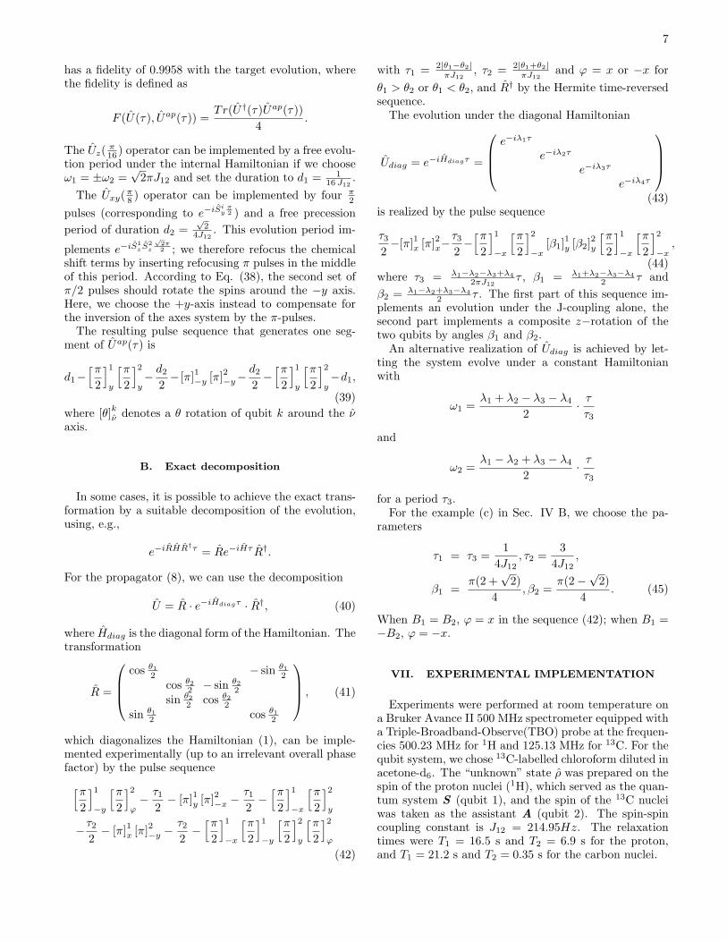
has a fidelity of 0.9958 with the target evolution, wherethe fidelity is defined as

F (U(τ), Uap(τ)) =Tr(U†(τ)Uap(τ))

4.

The Uz( π16 ) operator can be implemented by a free evolu-tion period under the internal Hamiltonian if we chooseω1 = ±ω2 =

√2πJ12 and set the duration to d1 = 1

16 J12.

The Uxy(π8 ) operator can be implemented by four π2

pulses (corresponding to e−iSiyπ2 ) and a free precession

period of duration d2 =√

24J12

. This evolution period im-

plements e−iS1z S

2z

√2π2 ; we therefore refocus the chemical

shift terms by inserting refocusing π pulses in the middleof this period. According to Eq. (38), the second set ofπ/2 pulses should rotate the spins around the −y axis.Here, we choose the +y-axis instead to compensate forthe inversion of the axes system by the π-pulses.

The resulting pulse sequence that generates one seg-ment of Uap(τ) is

d1−[π

2

]1y

[π2

]2y− d2

2− [π]1−y [π]2−y−

d2

2−[π

2

]1y

[π2

]2y−d1,

(39)where [θ]kν denotes a θ rotation of qubit k around the νaxis.

B. Exact decomposition

In some cases, it is possible to achieve the exact trans-formation by a suitable decomposition of the evolution,using, e.g.,

e−iRHR†τ = Re−iHτ R†.

For the propagator (8), we can use the decomposition

U = R · e−iHdiagτ · R†, (40)

where Hdiag is the diagonal form of the Hamiltonian. Thetransformation

R =

cos θ12 − sin θ1

2

cos θ22 − sin θ22

sin θ22 cos θ22

sin θ12 cos θ12

, (41)

which diagonalizes the Hamiltonian (1), can be imple-mented experimentally (up to an irrelevant overall phasefactor) by the pulse sequence[π

2

]1−y

[π2

]2ϕ− τ1

2− [π]1y [π]2−x −

τ12−[π

2

]1−x

[π2

]2y

−τ22− [π]1x [π]2−y −

τ22−[π

2

]1−x

[π2

]1−y

[π2

]2y

[π2

]2ϕ

(42)

with τ1 = 2|θ1−θ2|πJ12

, τ2 = 2|θ1+θ2|πJ12

and ϕ = x or −x forθ1 > θ2 or θ1 < θ2, and R† by the Hermite time-reversedsequence.

The evolution under the diagonal Hamiltonian

Udiag = e−iHdiagτ =

e−iλ1τ

e−iλ2τ

e−iλ3τ

e−iλ4τ

(43)

is realized by the pulse sequence

τ32−[π]1x [π]2x−

τ32−[π

2

]1−x

[π2

]2−x

[β1]1y [β2]2y[π

2

]1−x

[π2

]2−x,

(44)where τ3 = λ1−λ2−λ3+λ4

2πJ12τ , β1 = λ1+λ2−λ3−λ4

2 τ andβ2 = λ1−λ2+λ3−λ4

2 τ . The first part of this sequence im-plements an evolution under the J-coupling alone, thesecond part implements a composite z−rotation of thetwo qubits by angles β1 and β2.

An alternative realization of Udiag is achieved by let-ting the system evolve under a constant Hamiltonianwith

ω1 =λ1 + λ2 − λ3 − λ4

2· ττ3

and

ω2 =λ1 − λ2 + λ3 − λ4

2· ττ3

for a period τ3.For the example (c) in Sec. IV B, we choose the pa-

rameters

τ1 = τ3 =1

4J12, τ2 =

34J12

,

β1 =π(2 +

√2)

4, β2 =

π(2−√

2)4

. (45)

When B1 = B2, ϕ = x in the sequence (42); when B1 =−B2, ϕ = −x.

VII. EXPERIMENTAL IMPLEMENTATION

Experiments were performed at room temperature ona Bruker Avance II 500 MHz spectrometer equipped witha Triple-Broadband-Observe(TBO) probe at the frequen-cies 500.23 MHz for 1H and 125.13 MHz for 13C. For thequbit system, we chose 13C-labelled chloroform diluted inacetone-d6. The “unknown” state ρ was prepared on thespin of the proton nuclei (1H), which served as the quan-tum system S (qubit 1), and the spin of the 13C nucleiwas taken as the assistant A (qubit 2). The spin-spincoupling constant is J12 = 214.95Hz. The relaxationtimes were T1 = 16.5 s and T2 = 6.9 s for the proton,and T1 = 21.2 s and T2 = 0.35 s for the carbon nuclei.

8

A. Experimental procedure

There are three steps to implement the measurementscheme stated above: (i) Preparation of the initial sys-tem, (ii) Quantum simulation and (iii) Measurement.

Any qubit state ρ = 121 + ~s · ~S can be parameterized

as a vector in the Bloch sphere:

~s(r, θ, φ) = (sx, sy, sz)T

= (r sin θ cosφ, r sin θ cosφ, r cos θ)T , (46)

where the amplitude r = 1 for a pure state, and 0 ≤ r < 1for mixed states and θ, and φ are, respectively, the polarand azimuthal angles.

The combined system was initialized in the state %0 =ρ(S) ⊗ ξ(A). In our demonstration experiment we chosea completely disordered state ξ = 1

21(A) that is exper-

imentally easy to prepare. Such an initial state %0 =ρ(S) ⊗ 1

21(A) was prepared by the NMR pulse sequence:

[arccos (r)]1y[π

2

]2y−Gz − [θ]1φ+π/2 . (47)

The first two RF pulses define the amount of spin po-larization on the two qubits. The field gradient pulseGz dephases transverse magnetization to eliminate off-diagonal terms in the density operator. The last RFpulse turns the remaining (longitudinal) magnetizationof qubit 1 into the desired orientation. The result ofthe preparation was checked using the standard methodof state determination based on three noncommutativemeasurements of the system S , i.e., σ(S)

x , σ(S)y and σ(S)

z .The experimental results are plotted in Fig. 5 c) and d)for r = 1 and 1

2 . The experimental average fidelity isabove 0.99.

For the coupling Hamiltonian that transfers the infor-mation from S to A, we chose Hopt of example (c) (sec-tion IV B). We performed two different methods for thesimulation of this propagator (8): the“short period ex-pansion” (see section VI A), using the sequence (39) withm = 2, and the exact decomposition (40) (see section VIB) with the NMR pulse sequences (42) and (44).

After the coupling evolution, we measured the x com-ponents of the two spins to obtain the joint probabilitiesPkq. For this purpose, we rotated the spins to the z-axis,using a

[π2

]1,2y

pulse and destroyed off-diagonal elementsby a magnetic field gradient pulse Gz. The populationscould then be measured by applying another rf pulse toeach of the spins and measuring their free induction de-cays (FIDs). If the two spins are different isotopes, asin our case, their FIDs usually have to be measured inseparate experiments.

The resulting pulse sequence for the readout is thus[π2

]1,2−y−Gz −

[π2

]iy− FIDi. (48)

where i = 1 or 2 denotes qubit i. The measured FIDsalong with the normalization condition (

∑kq Pkq = 1) al-

lowed us to reconstruct the four diagonal elements (pop-ulations) in the density matrix, which correspond to fourjoint probabilities Pkq. The information about the stateρ was then obtained by the inverse mapping M−1.

B. Experimental Results

x

y

z

x

y

z

(b)

x

y

z

NMR Signal

NMR Signal

NMR Signal

FIG. 4: Experimental NMR spectra of carbon and proton fordifferent initial conditions. φ = 0 and (a) θ = 0, (b) θ = π/2and (c) θ = π. The y-axis denotes the signal amplitude inarbitrary units.

Figure 4 shows the experimentally observed NMR sig-nals after Fourier transformation of the correspondingFIDs for the proton and carbon spins for the follow-ing initial states: (a) θ = 0 (i.e. ρ = 1

21 + Sz), (b)φ = 0, θ = π/2 (i.e., ρ = 1

21 + Sx), (c) θ = π (i.e.,ρ = 1

21− Sz).The amplitudes of the different resonance lines corre-

spond directly to population differences:

SNMR(Proton) ∼ P1µ − P2µ

SNMR(Carbon) ∼ Pµ1 − Pµ2,(49)

where µ = 1 for the resonance line with positive fre-quency and µ = 2 for the negative frequency line. Fromthese populations, we determine the initial condition byinverting Eq. (12).

Fig. 5 summarizes these results for a series of similarexperiments, where we chose initial conditions ~s (r, θ, φ)

9

090

180 0 180 360−1

0

1

φθ

s x(exp)

090

180 0 180 360−1

0

1

φ

(a)

θ

s y(exp)

090

180 0 180 360−1

0

1

φθ

s z(exp)

090

180 0 180 360−1

0

1

φθ

s x(exp)

090

180 0 180 360−1

0

1

φ

(b)

θ

s y(exp)

090

180 0 180 360−1

0

1

φθ

s z(exp)

090

180 0 180 360−1

0

1

φθ

s x(tom)

090

180 0 180 360−1

0

1

φ

(c)

θ

s y(tom)

090

180 0 180 360−1

0

1

φθ

s z(tom)

090

180 0 180 360−1

0

1

φθ

s x(tom)

090

180 0 180 360−1

0

1

φ

(d)

θ

s y(tom)

090

180 0 180 360−1

0

1

φθ

s z(tom)

FIG. 5: (Color Online) Experimental quantum state tomog-raphy for the general initial state ~s(r, θ, φ) [see Eq. (46)]. Wecompare the results from measuring a single observable of thecombined system S+A (rows (a) and (b)) with the resultsfrom the conventional measurement scheme using three non-commutative measurements of the system S (rows (c) and(d)). In both cases, the expectation values sx, sy, sz, areshown from left to right as functions of the angles θ and φ:(a) and (c) for a pure state (r = 1) and (b) and (d) for apartially mixed state with r = 1

2.

varying θ from 0 to π in increments of π/8, and φ from 0to 2π with an increment of π/12. In Fig. 5a, we show themeasured components s(exp)

x , s(exp)y , s

(exp)z for pure states

(r = 1), while (b) shows the corresponding results formixed states with r = 1

2 . The experiments cover a widerange of points on and within the Bloch sphere. Theexperimental results clearly show the expected cosine andsine modulations (46), indicating that the measurementnetwork is effective for all these input states. The averagefidelity over all N = 9× 13 measured states is

Fav =1N

N∑1

Tr(ρinρexp)√Tr(ρ2

in)Tr(ρ2exp)

≈ 0.99

for both cases, r = 1 and r = 12 .

The experimental data shown in Fig. 5 were obtainedwith the “short period expansion” technique of sectionVI A, i.e., the propagator U(τ) was approximately real-ized by Eq. (37) by repeating the sequence (39) twice.We also repeated the experiment with the “exact decom-position” technique. The propagator U(τ) was realizedby the exact decomposition Eq. (40). The corresponding

pulse sequence was obtained by combining the sequences(42) with (44). The results that we obtained were simi-lar to those represented in Fig. 5, but the fidelities wereslightly lower. This difference is probably due to thelarger number of pulses in this experiment.

C. Precision of the Measurement

An alternative measure of the precision of the mea-surement is the distance D between the experimentallydetermined state ~sexp and the ”true” input state ~s. Interms of the parametrization (46), the trace distance be-tween the two density operators is

D(~sexp, ~s) =|~sexp − ~s|

2=

12

√∆s2

x + ∆s2y + ∆s2

z (50)

where ∆sν = s(exp)ν − sν(ν = x, y, z).

Writing ∆P for the experimental errors and using thedefinition (12) of the transfer matrix, we find for the dis-tance

D(~sexp, ~s) = E|∆P |, (51)

where

E =12

√E2x + E2

y + E2z (52)

and

Ex = ∆sx∆P = 1

det(M)

∑4k=1Ak2

Ey = ∆sx∆P = 1

det(M)

∑4k=1Ak3

Ez = ∆sx∆P = 1

det(M)

∑4k=1Ak4

. (53)

The Akj are the cofactors of the minors Mkj of the trans-fer matrix

M =12M

1 0 0 10 1 −i 00 1 i 01 0 0 −1

.

The determinant of this matrix is det(M) = − 14 i∆.

Therefore, the error propagation coefficients Eα dependonly on the mappingM. The smaller they are, the higherthe precision of the resulting measurement.

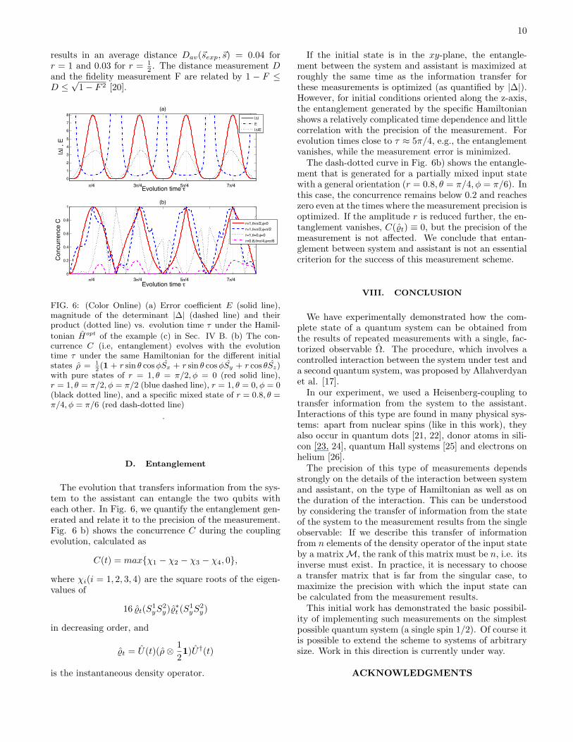
As Eq. (53) shows, the error propagation scales in-versely with the determinant ∆ of the transfer matrixM. We illustrate this dependence in Fig. 6a), where weplot the two quantities as a function of the coupling evo-lution time τ . The minima of E occur near the maximaof |∆|, and when |∆| = 0, E tends to infinity. In thisrange, it is impossible to determine the state ρ by sucha measurement. A closer look shows that the minimaof E do not occur exactly at the maxima of |∆|. Thedifference arises from the numerators in (53).

In our experiment, the experimental uncertainties are∆P ≈ 5%. For the chosen experimental parameters, this

10

results in an average distance Dav(~sexp, ~s) = 0.04 forr = 1 and 0.03 for r = 1

2 . The distance measurement Dand the fidelity measurement F are related by 1 − F ≤D ≤

√1− F 2 [20].

0

1

2

3

4

5

6

7

8(a)

|Δ| ,

E

Evolution time τπ/4 3π/4 5π/4 7π/4

|Δ|E|Δ|E

0

0.2

0.4

0.6

0.8

1(b)

Conc

urre

nce

C

Evolution time τπ/4 3π/4 5π/4 7π/4

r=1,θ=π/2,φ=0r=1,θ=π/2,φ=π/2r=1,θ=0,φ=0r=0.8,θ=π/4,φ=π/6

FIG. 6: (Color Online) (a) Error coefficient E (solid line),magnitude of the determinant |∆| (dashed line) and theirproduct (dotted line) vs. evolution time τ under the Hamil-

tonian Hopt of the example (c) in Sec. IV B. (b) The con-currence C (i.e, entanglement) evolves with the evolutiontime τ under the same Hamiltonian for the different initialstates ρ = 1

2(1 + r sin θ cosφSx + r sin θ cosφSy + r cos θSz)

with pure states of r = 1, θ = π/2, φ = 0 (red solid line),r = 1, θ = π/2, φ = π/2 (blue dashed line), r = 1, θ = 0, φ = 0(black dotted line), and a specific mixed state of r = 0.8, θ =π/4, φ = π/6 (red dash-dotted line)

.

D. Entanglement

The evolution that transfers information from the sys-tem to the assistant can entangle the two qubits witheach other. In Fig. 6, we quantify the entanglement gen-erated and relate it to the precision of the measurement.Fig. 6 b) shows the concurrence C during the couplingevolution, calculated as

C(t) = maxχ1 − χ2 − χ3 − χ4, 0,

where χi(i = 1, 2, 3, 4) are the square roots of the eigen-values of

16 %t(S1yS

2y)%∗t (S

1yS

2y)

in decreasing order, and

%t = U(t)(ρ⊗ 121)U†(t)

is the instantaneous density operator.

If the initial state is in the xy-plane, the entangle-ment between the system and assistant is maximized atroughly the same time as the information transfer forthese measurements is optimized (as quantified by |∆|).However, for initial conditions oriented along the z-axis,the entanglement generated by the specific Hamiltonianshows a relatively complicated time dependence and littlecorrelation with the precision of the measurement. Forevolution times close to τ ≈ 5π/4, e.g., the entanglementvanishes, while the measurement error is minimized.

The dash-dotted curve in Fig. 6b) shows the entangle-ment that is generated for a partially mixed input statewith a general orientation (r = 0.8, θ = π/4, φ = π/6). Inthis case, the concurrence remains below 0.2 and reacheszero even at the times where the measurement precision isoptimized. If the amplitude r is reduced further, the en-tanglement vanishes, C(%t) ≡ 0, but the precision of themeasurement is not affected. We conclude that entan-glement between system and assistant is not an essentialcriterion for the success of this measurement scheme.

VIII. CONCLUSION

We have experimentally demonstrated how the com-plete state of a quantum system can be obtained fromthe results of repeated measurements with a single, fac-torized observable Ω. The procedure, which involves acontrolled interaction between the system under test anda second quantum system, was proposed by Allahverdyanet al. [17].

In our experiment, we used a Heisenberg-coupling totransfer information from the system to the assistant.Interactions of this type are found in many physical sys-tems: apart from nuclear spins (like in this work), theyalso occur in quantum dots [21, 22], donor atoms in sili-con [23, 24], quantum Hall systems [25] and electrons onhelium [26].

The precision of this type of measurements dependsstrongly on the details of the interaction between systemand assistant, on the type of Hamiltonian as well as onthe duration of the interaction. This can be understoodby considering the transfer of information from the stateof the system to the measurement results from the singleobservable: If we describe this transfer of informationfrom n elements of the density operator of the input stateby a matrixM, the rank of this matrix must be n, i.e. itsinverse must exist. In practice, it is necessary to choosea transfer matrix that is far from the singular case, tomaximize the precision with which the input state canbe calculated from the measurement results.

This initial work has demonstrated the basic possibil-ity of implementing such measurements on the simplestpossible quantum system (a single spin 1/2). Of course itis possible to extend the scheme to systems of arbitrarysize. Work in this direction is currently under way.

ACKNOWLEDGMENTS

11

We gratefully acknowledge helpful discussions with Dr.Bo Chong, Dr. Jingfu Zhang and financial support fromthe DFG through Su 192/19-1. Du. J thanks the support

of NSFC of China, CAS and the European Commissionunder Contract No. 007065 (Marie Curie).

[1] W. Pauli, in Handbuch der Physik, edited by H. Geigerand K. Scheel (Springer, Berlin, 1933), vol. 24, p. 98.

[2] N. Bohr, Phys. Rev. 48, 696 (1935).[3] C. W. Helstrom, Quantum Detection and Estimation

Theory (Academic Press, New York, 1976).[4] A. Chefles, Contemporary Physics 41, 401 (2000).[5] R. Gill and M. Guta, arXiv.org:quant-ph/0303020

(2003).[6] H. Bechmann-Pasquinucci and W. Tittel, Phys. Rev. A

61, 062308 (2000).[7] H. Bechmann-Pasquinucci and A. Peres, Phys. Rev. Lett.

85, 3313 (2000).[8] D. Welsch, W. Vogel, and T. Opatrny, Progr. Opt. 39,

63 (1999).[9] G. D’Ariano, In: T. HakioImagelu and A.S. Shumovsky,

Editors, Quantum Optics and Spectroscopy of Solids, Ed-itors, Kluwer, Amsterdam pp. 175–202 (1997).

[10] U. Leonhardt, Measuring the Quantum State of Light(Cambridge University Press, New York, 1997).

[11] I. D. Ivonovic, J. Phys. A: Math. Gen. 14, 3241 (1981).[12] W. K. Wootters and B. D. Fields, Ann. Phys. 191, 363

(1989).[13] J. Rehacek, B.-G. Englert, and D. Kaszlikowski, Phys.

Rev. A 70, 052321 (2004).[14] G. M. D’Ariano, Phys. Lett. A 300, 1 (2002).[15] C. M. Caves, C. A. Fuchs, and R. Schack, Journal

of Mathematical Physics 43, 4537 (2002), URL http:

//link.aip.org/link/?JMP/43/4537/1.[16] J. Du, M. Sun, X. Peng, and T. Durt, Phys. Rev. A 74,

042341 (2006).[17] A. E. Allahverdyan, R. Balian, and T. M. Nieuwenhuizen,

Phys. Rev. Lett. 92, 120402 (2004).[18] R. R. Ernst, G. Bodenhausen, and A. Wokaun, Prin-

ciples of Nuclear Magnetic Resonance in One and TwoDimensions (Oxford University Press, Oxford, 1994).

[19] H. Trotter, Proc. Amer. Math. Soc. 10, 545 (1959).[20] M. A. Nielsen and I. L. Chuang, Quantum Computa-

tion and Quantum Information (Cambridge Univ. Press,Cambridge, 2000).

[21] D. Loss and D. P. DiVincenzo, Phys. Rev. A 57, 120(1998).

[22] A. Imamogu, D. D. Awschalom, G. Burkard, D. P. Di-Vincenzo, D. Loss, M. Sherwin, and A. Small, Phys. Rev.Lett. 83, 4204 (1999).

[23] B. E. Kane, Nature 393, 133 (1998).[24] R. Vrijen, E. Yablonovitch, K. Wang, H. W. Jiang, A. Ba-

landin, V. Roychowdhury, T. Mor, and D. DiVincenzo,Phys. Rev. A 62, 012306 (2000).

[25] D. Mozyrsky, V. Privman, and M. L. Glasser, Phys. Rev.Lett. 86, 5112 (2001).

[26] M. Dykman and P. Platzman, Fortschritte der Physik48, 1095 (2000).