Optimisation of radial basis function neural networks using biharmonic spline interpolation
13
Ž . Chemometrics and Intelligent Laboratory Systems 41 1998 17–29 Optimisation of radial basis function neural networks using biharmonic spline interpolation John Tetteh a , Sian Howells a , Ed Metcalfe a, ) , Takahiro Suzuki b a School of Chemical and Life Sciences, UniÕersity of Greenwich, London SE18 6PF, UK b Research Laboratory of Resources Utilization, Tokyo Institute of Technology, 4259 Nagatsuta, Midori-ku, Yokohama 226, Japan Received 20 January 1998; accepted 5 March 1998 Abstract Biharmonic spline interpolation has been applied as an optimisation tool to study response surfaces of bi-directional data. Both regularly and randomly spaced training data yielded results with prediction errors in the range 0.1 to 10%. Practical application of the technique has been demonstrated by optimising both the spread parameter and the number of neurons in Ž . the hidden layer of radial basis function RBF neural networks. The efficiency and practical application of this optimisation Ž . approach is demonstrated by the prediction of the auto-ignition temperature AIT values of 232 organic compounds using Ž . quantitative structure–property relationships QSPR with six descriptors. It is concluded that this optimisation strategy is fast and provides a very flexible way of modelling non-linear systems in general. q 1998 Elsevier Science B.V. All rights reserved. Keywords: Splines; Green’s function; Response surface; Optimisation; Neural networks; Radial basis functions 1. Introduction Determination of the optimum configuration or condition of a system generally requires a systematic and well-planned set of experiments, using experi- mental design andror response surface methodolo- w x gies 1,2 . This approach has been used extensively in several scientific disciplines such as the optimisation of chemical reaction conditions to achieve higher wx yield, or a target property of a product 3 . The broad ) Corresponding author. aim of such experiments is to explore the simultane- ous optimisation of two or more factors, x which iyn Ž together influence an expected response, Z n Ž x . iyn . input dimension . Generally the optimum search re- quires an initial training set, carefully selected to lie within the expected boundary limits of the system under investigation, while spanning the experimental data range. The target outputs from these experimen- tal points, which should be statistically reproducible, are used as valuable knowledge to interpolate and predict the likely behaviour of the system within the parameter boundary limits. The mapping of experi- mental data points to the targets is generally per- 0169-7439r98r$19.00 q 1998 Elsevier Science B.V. All rights reserved. Ž . PII S0169-7439 98 00035-5
-
Upload
instituteforsustainbility -
Category
Documents
-
view
4 -
download
0
Transcript of Optimisation of radial basis function neural networks using biharmonic spline interpolation

Ž .Chemometrics and Intelligent Laboratory Systems 41 1998 17–29
Optimisation of radial basis function neural networks usingbiharmonic spline interpolation
John Tetteh a, Sian Howells a, Ed Metcalfe a,), Takahiro Suzuki b
a School of Chemical and Life Sciences, UniÕersity of Greenwich, London SE18 6PF, UKb Research Laboratory of Resources Utilization, Tokyo Institute of Technology, 4259 Nagatsuta, Midori-ku, Yokohama 226, Japan
Received 20 January 1998; accepted 5 March 1998
Abstract
Biharmonic spline interpolation has been applied as an optimisation tool to study response surfaces of bi-directional data.Both regularly and randomly spaced training data yielded results with prediction errors in the range 0.1 to 10%. Practicalapplication of the technique has been demonstrated by optimising both the spread parameter and the number of neurons in
Ž .the hidden layer of radial basis function RBF neural networks. The efficiency and practical application of this optimisationŽ .approach is demonstrated by the prediction of the auto-ignition temperature AIT values of 232 organic compounds using
Ž .quantitative structure–property relationships QSPR with six descriptors. It is concluded that this optimisation strategy isfast and provides a very flexible way of modelling non-linear systems in general. q 1998 Elsevier Science B.V. All rightsreserved.
Keywords: Splines; Green’s function; Response surface; Optimisation; Neural networks; Radial basis functions
1. Introduction
Determination of the optimum configuration orcondition of a system generally requires a systematicand well-planned set of experiments, using experi-mental design andror response surface methodolo-
w xgies 1,2 . This approach has been used extensively inseveral scientific disciplines such as the optimisationof chemical reaction conditions to achieve higher
w xyield, or a target property of a product 3 . The broad
) Corresponding author.
aim of such experiments is to explore the simultane-ous optimisation of two or more factors, x whichiyn
Žtogether influence an expected response, Z nŽ x .iy n
.input dimension . Generally the optimum search re-quires an initial training set, carefully selected to liewithin the expected boundary limits of the systemunder investigation, while spanning the experimentaldata range. The target outputs from these experimen-tal points, which should be statistically reproducible,are used as valuable knowledge to interpolate andpredict the likely behaviour of the system within theparameter boundary limits. The mapping of experi-mental data points to the targets is generally per-
0169-7439r98r$19.00 q 1998 Elsevier Science B.V. All rights reserved.Ž .PII S0169-7439 98 00035-5

( )J. Tetteh et al.rChemometrics and Intelligent Laboratory Systems 41 1998 17–2918
formed so that non-linear trends are captured. Mostnon-linear mapping involves quadratic polynomialsw x4 , but a major limitation of quadratic interpolationis the inability to cope with wide boundary limits. Asa result several boundary limits may need to be ex-amined step by step in an effort to locate the area ofoptimum response. This is very time consuming whenthe surface is strongly non-linear. Besides it is verydifficult to know if a local non-optimum region hasbeen located.
The employment of biharmonic splines in this pa-per aims to develop a faster method of locating theoptimum within wide boundary limits and also to ex-amine the modelling accuracy of highly non-linear
Ž .systems by radial basis function RBF neural net-works. The importance of neural network optimisa-tion has prompted others to study and propose strate-gies and algorithms to achieve this. Berthold and Di-
w xamond 5 proposed an algorithm which automati-cally adjusts the spread parameter, for a fixed num-ber of neurons in the hidden layer, during training ofRBF networks with Gaussian functions. This ap-proach yielded significantly reduced training speedsin comparison with backpropagation and also fixedspread RBF neural networks when used for imageidentification. In this paper we extend their work fur-
ther to the simultaneous optimisation of both theŽ .spread parameter s and the number of hidden layer
Ž .neurons n . A theoretical report on optimal experi-mental design in neural networks has also been re-
w xported by D.A. Cohn 6 . He showed that a system-atic optimisation of neural networks via experimentaldesign minimises generalisation errors because themodelling domain is explored efficiently and com-pletely when inputs and targets are explicitly de-
w xfined. In our previous study 7 , the number of neu-rons and spread of the RBF network were optimisedusing a quadratic response surface generated from a32 factorial design points. The optimum networkconfiguration was obtained after performing a seriesof experiments based on knowledge from the last ex-periment.
The inspiration for this paper is from the work byw xSandwell 8 . He developed the biharmonic spline in-
terpolation technique and applied it to satellite al-timeter data to predict the geoid height map of theCaribbean area to identify new features in theseoceans such as geoid asymmetrics and parallel lin-eations to the Beata Ridge which extends from CostaRica to the eastern edge of Jamaica. A full theoreti-cal outline of splines and their applications has been
w xdocumented in the literature 9,10 . An overview of
Ž .Fig. 1. Schematic of biharmonic function w x that passes through the data points w located at x found by applying point forces a to ai i jw xthin elastic beam or spline 7 .

( )J. Tetteh et al.rChemometrics and Intelligent Laboratory Systems 41 1998 17–29 19
Table 1Biharmonic green functions
Number of Green function: Gradient ofŽ .dimensions: m f x green function:m
Ž .=f xm
3< < < <1 x x x< < Ž < < . Ž < < .2 x 2 ln x y1 x 2 ln x y1
y1< < < <3 x x xy2< < < <4 ln x x x
y1 y3< < < <5 x y x xy2 y4< < < <6 x y2 x x4y m 2ym< < Ž . < <m x 4y m x x
the biharmonic spline algorithm after Sandwell usedin this paper is presented below.
2. Overview of biharmonic splines interpolation
ŽThe general relationship between a two factor x. Ž . Ž . Ž .and y model with data points xy , xy , . . . xy1 2 N
and a target response z may be expressed asŽ x y.
z sF xy , xy , . . . , xy qe 1Ž . Ž . Ž . Ž .1 2 NŽ x y.
e is the error in the model. N is the number of sam-Ž .ples. Eq. 1 is a two-dimensional regression map-
ping xy onto z . The goal is to determine the rela-Ž x y.tionship F given a representative set of z and xy.Ž x y.Once this relationship has been established, interpo-
Ž .lation or extrapolation can be done within the ex-perimental limits of x and y to obtain the full re-sponse surface Z. The method by which F is estab-lished is the analytical challenge. The general strat-egy is to employ a method capable of capturing bothlinear and non-linear features of the response. Oncethe response surface has been generated vital strate-gic decisions on the model can be made. In compari-son with a quadratic response approach which onlyworks well within narrow boundaries, the spline in-terpolation is attractive because it is capable of han-
Ž . Ž .Fig. 2. RBF network architecture with detail of hidden layer neurons n and spread parameter s .
( )J. Tetteh et al.rChemometrics and Intelligent Laboratory Systems 41 1998 17–2920
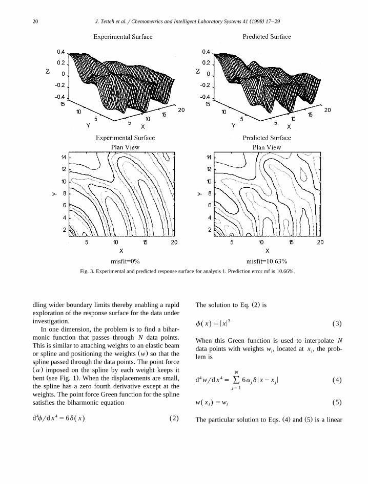
Fig. 3. Experimental and predicted response surface for analysis 1. Prediction error mf is 10.66%.
dling wider boundary limits thereby enabling a rapidexploration of the response surface for the data underinvestigation.
In one dimension, the problem is to find a bihar-monic function that passes through N data points.This is similar to attaching weights to an elastic beam
Ž .or spline and positioning the weights w so that thespline passed through the data points. The point forceŽ .a imposed on the spline by each weight keeps it
Ž .bent see Fig. 1 . When the displacements are small,the spline has a zero fourth derivative except at theweights. The point force Green function for the splinesatisfies the biharmonic equation
d4frd x 4 s6d x 2Ž . Ž .
Ž .The solution to Eq. 2 is
< < 3f x s x 3Ž . Ž .
When this Green function is used to interpolate Ndata points with weights w , located at x , the prob-i i
lem is
N4 4 < <d wrd x s 6a d xyx 4Ž .Ý j j
js1
w x sw 5Ž . Ž .i i
Ž . Ž .The particular solution to Eqs. 4 and 5 is a linear

( )J. Tetteh et al.rChemometrics and Intelligent Laboratory Systems 41 1998 17–29 21
Fig. 4. Experimental and predicted response surface for analysis 2. Prediction error mf is 6.27%.
combination of point force Green functions centred ateach point.
N3< <w x s a xyx 6Ž . Ž .Ý j j
js1
The strength of each point force a , is found byj
solving the linear system
N3< <w s a x yx 7Ž .Ýi j i j
js1
If the slopes, s are used rather than the x values,i i
then the a ’s are determined by solving the follow-j
ing linear systems:N
< <s s3 a x yx x yx 8Ž . Ž .Ýi j i j i jjs1
Once the a ’s are determined, the biharmonic func-jŽ . Ž .tion w x can be evaluated at any point using Eq. 6 .
In two or more dimensions the derivatives aresimilar to those for one-dimension. For N data pointsin m dimensions the problem is
N4= w x s a d xyx 9Ž . Ž . Ž .Ý j j
js1
w x sw 10Ž . Ž .i i
( )J. Tetteh et al.rChemometrics and Intelligent Laboratory Systems 41 1998 17–2922
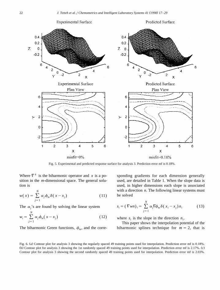
Fig. 5. Experimental and predicted response surface for analysis 3. Prediction error mf is 0.18%.
Where = 4 is the biharmonic operator and x is a po-sition in the m-dimensional space. The general solu-tion is
N
w x s a f d xyx 11Ž . Ž . Ž .Ý j m jjs1
The a ’s are found by solving the linear systemj
N
w s a f xyx 12Ž . Ž .Ýi j m jjs1
The biharmonic Green functions, f , and the corre-m
sponding gradients for each dimension generallyused, are detailed in Table 1. When the slope data isused, in higher dimensions each slope is associatedwith a direction n. The following linear systems mustbe solved
N
s s = wn s a =f d x yx n 13Ž . Ž . Ž .Ýii j m i j ijs1
where s is the slope in the direction n .i i
This paper shows the interpolation potential of thebiharmonic splines technique for m s 2, that is
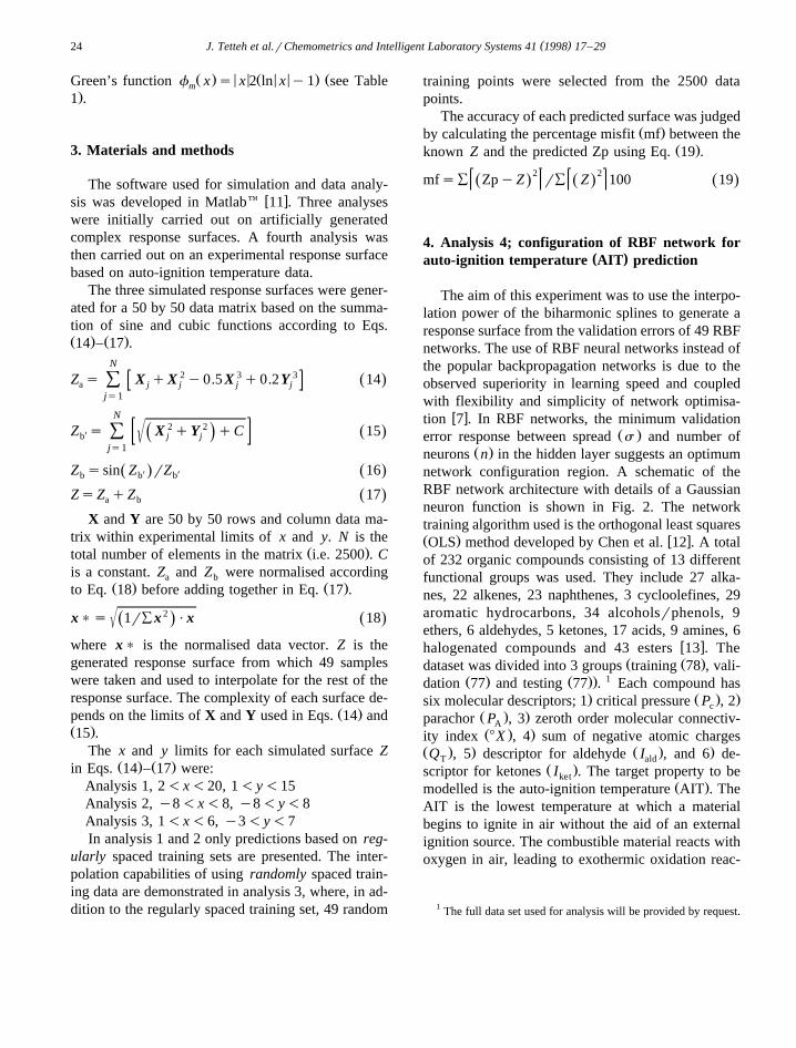
Ž .Fig. 6. a Contour plot for analysis 3 showing the regularly spaced 49 training points used for interpolation. Prediction error mf is 0.18%.Ž . Ž .b Contour plot for analysis 3 showing the 1st randomly spaced 49 training points used for interpolation. Prediction error mf is 2.17%. cContour plot for analysis 3 showing the second randomly spaced 49 training points used for interpolation. Prediction error mf is 2.03%.

( )J. Tetteh et al.rChemometrics and Intelligent Laboratory Systems 41 1998 17–29 23
( )J. Tetteh et al.rChemometrics and Intelligent Laboratory Systems 41 1998 17–2924
Ž . < < Ž < < . ŽGreen’s function f x s x 2 ln x y1 see Tablem.1 .
3. Materials and methods
The software used for simulation and data analy-w xsis was developed in Matlabe 11 . Three analyses
were initially carried out on artificially generatedcomplex response surfaces. A fourth analysis wasthen carried out on an experimental response surfacebased on auto-ignition temperature data.
The three simulated response surfaces were gener-ated for a 50 by 50 data matrix based on the summa-tion of sine and cubic functions according to Eqs.Ž . Ž .14 – 17 .
N2 3 3Z s X qX y0.5 X q0.2Y 14Ž .Ýa j j j j
js1
N2 2
XZ s X qY qC 15Ž .(Ž .Ýb j jjs1
Z ssin Z X rZ X 16Ž . Ž .b b b
ZsZ qZ 17Ž .a b
X and Y are 50 by 50 rows and column data ma-trix within experimental limits of x and y. N is the
Ž .total number of elements in the matrix i.e. 2500 . Cis a constant. Z and Z were normalised accordinga b
Ž . Ž .to Eq. 18 before adding together in Eq. 17 .
2(x)s 1rÝx Px 18Ž .Ž .where x) is the normalised data vector. Z is thegenerated response surface from which 49 sampleswere taken and used to interpolate for the rest of theresponse surface. The complexity of each surface de-
Ž .pends on the limits of X and Y used in Eqs. 14 andŽ .15 .
The x and y limits for each simulated surface ZŽ . Ž .in Eqs. 14 – 17 were:
Analysis 1, 2-x-20, 1-y-15Analysis 2, y8-x-8, y8-y-8Analysis 3, 1-x-6, y3-y-7In analysis 1 and 2 only predictions based on reg-
ularly spaced training sets are presented. The inter-polation capabilities of using randomly spaced train-ing data are demonstrated in analysis 3, where, in ad-dition to the regularly spaced training set, 49 random
training points were selected from the 2500 datapoints.
The accuracy of each predicted surface was judgedŽ .by calculating the percentage misfit mf between the
Ž .known Z and the predicted Zp using Eq. 19 .2 2mfsÝ ZpyZ rÝ Z 100 19Ž . Ž . Ž .
4. Analysis 4; configuration of RBF network for( )auto-ignition temperature AIT prediction
The aim of this experiment was to use the interpo-lation power of the biharmonic splines to generate aresponse surface from the validation errors of 49 RBFnetworks. The use of RBF neural networks instead ofthe popular backpropagation networks is due to theobserved superiority in learning speed and coupledwith flexibility and simplicity of network optimisa-
w xtion 7 . In RBF networks, the minimum validationŽ .error response between spread s and number of
Ž .neurons n in the hidden layer suggests an optimumnetwork configuration region. A schematic of theRBF network architecture with details of a Gaussianneuron function is shown in Fig. 2. The networktraining algorithm used is the orthogonal least squaresŽ . w xOLS method developed by Chen et al. 12 . A totalof 232 organic compounds consisting of 13 differentfunctional groups was used. They include 27 alka-nes, 22 alkenes, 23 naphthenes, 3 cycloolefines, 29aromatic hydrocarbons, 34 alcoholsrphenols, 9ethers, 6 aldehydes, 5 ketones, 17 acids, 9 amines, 6
w xhalogenated compounds and 43 esters 13 . TheŽ Ž .dataset was divided into 3 groups training 78 , vali-
Ž . Ž .. 1dation 77 and testing 77 . Each compound has. Ž . .six molecular descriptors; 1 critical pressure P , 2c
Ž . .parachor P , 3 zeroth order molecular connectiv-AŽ . .ity index 8X , 4 sum of negative atomic charges
Ž . . Ž . .Q , 5 descriptor for aldehyde I , and 6 de-T aldŽ .scriptor for ketones I . The target property to beket
Ž .modelled is the auto-ignition temperature AIT . TheAIT is the lowest temperature at which a materialbegins to ignite in air without the aid of an externalignition source. The combustible material reacts withoxygen in air, leading to exothermic oxidation reac-
1 The full data set used for analysis will be provided by request.

( )J. Tetteh et al.rChemometrics and Intelligent Laboratory Systems 41 1998 17–29 25

( )J. Tetteh et al.rChemometrics and Intelligent Laboratory Systems 41 1998 17–2926
tions. Auto-ignition occurs when the rate of heatevolved by these reactions is just greater than the rateat which heat is lost to the surroundings. It is used asan important fire performance parameter in combus-tion science. Accurate estimation of this parameter bya QSPR method can be cost-effective since current
w xlaboratory methods 14 are cumbersome and in somecases impossible due to the physical characteristics ofthe compound. A neural prediction of AIT by back-
w xpropagation networks was recently reported 15 . Inthis paper, a global model with satisfactory predic-tion capabilities was not obtained. Successful modelswere obtained when the data was sub classified ac-cording to functional groups. It is clear from this re-port that, obtaining a good model using backpropaga-tion networks was very time consuming since severaltrial models have to be examined. The problem is thatinitialisation of weights always depends on some op-timised random selection procedure during back-propagation training. It is difficult to compare the
w xwork in Ref. 15 to the results reported in this paperdue to differences in QSPR parameters used to modelthe AIT. We however show that the flexible optimi-sation capability of RBF neural networks has en-abled us to generate a single model for predicting AITfor temperatures ranging from 1708C to 6308C.
The input vectors used to characterise each com-Ž .pound were normalised by Eq. 18 . Data in the
training set was used to model the AIT. The valida-tion set was used to check the performance of themodel. The testing set was used only when the vali-dation error is optimised for the network by selectionof the optimum configuration from the biharmonicresponse surface. The training, validation and gener-ation of response surfaces together with the selectionof the optimum configuration were all automated. The
Ž . Ž .spread parameter s and the number of neurons nexamined were in the ranges 0.1-s-1 and 2-n-30 respectively. A typical training and optimisa-tion using 49 validation errors takes less than 10 minon a 166 MHz PC processor with a 16 MB RAM.
The calculation of network prediction perfor-mance is based on the average absolute error AE be-
Ž .tween Z and Zp values indicated in Eq. 20 .
5 5AEsÝ ZpyZ rn 20Ž .5 5P is the norm of the operation. n is the total num-ber of samples used.
5. Results and discussion
The known and predicted response surfaces foranalysis 1 and 2 are shown in Figs. 3 and 4. Thethree-dimensional view of the experimental datashows the complexity of the function but nonethelessthe predicted surfaces clearly describe the mainstructure of the surfaces quite well and this is shownmore clearly in the contour views. mf values of 10.6%and 6.3% for analysis 1 and 2 respectively are quitereasonable in view of the high degree of complexityof the surface.
In analysis 3 the surface was modelled very closelyand the level of misfit was only 0.17% when the 49
Ž .data training points were regularly spaced Fig. 5 ,reflecting the simpler structure of the surface over therange covered.
Two randomly spaced sets of training points werealso examined for analysis 3. Fig. 6a–c shows thetwo-dimensional contour views of the predicted re-sponse surfaces, together with the points selected forthe regularly spaced training data, and for the tworandomly spaced sets of training points. For theselatter experiments the errors were 2.17% and 2.03%respectively. Although in these cases the degree ofmodelling precision is an order of magnitude less thanfor regularly spaced points, the results do demon-strate that in situations where experimental datapoints cannot be regularly sampled due to practicallimitations, a reasonable estimation of the surface canstill be calculated.
The response surface for analysis 4 for the error inprediction of the AIT vs. s and n, using regularly
Ž .Fig. 7. a 3D overview of predicted error response surface for RBF neural models with arrow indicating region of minimum error and pos-Ž .sible optimum network configuration. b Contour overview of error response surface show validation error levels predicted with 49 regu-
Ž . Ž .larly spaced small open circles modelling points. Optimum network configuration found at spread s s0.931 and hidden layer neuronsŽ .n s9.

( )J. Tetteh et al.rChemometrics and Intelligent Laboratory Systems 41 1998 17–29 27
spaced training points for the RBF model errors, ispresented in Fig. 7. The experimental error in AIT isestimated to be "308C and it is notable that a fairlybroad area of the response surface models the experi-mental results well. For a good model, training, vali-
dation and testing errors should be similar to eachother and close to the experimental error. Poor mod-
Ž .elling is shown by validation or testing errors whichare higher than training or experimental errors, andthis is obtained with F7 neurons for any value of s ,
Ž .Fig. 8. a Training, validation, and testing results for optimum network configuration ss0.931 and ns9 selected from the response sur-Ž . Ž . Ž .face. Performance indicators: training v ; rs0.9088, errors30.28C. Validation I ; rs0.9129, errors30.18C. Testing ^ ; rs0.9280,
Ž . Ž .errors32.98C. b Training, validation and testing results for poorly configured network with ss0.20 and ns30. Training v ; rsŽ . Ž .0.9560, errors19.08C. Validation I ; rs0.5632, errors51.38C. Testing ^ ; rs0.4892, errors58.58C.

( )J. Tetteh et al.rChemometrics and Intelligent Laboratory Systems 41 1998 17–2928
or with )22 neurons and spread parameters belowŽabout 0.7. These two cases describe underfitting too
. Ž .few neurons and overfitting too many neurons ofthe data respectively.
The combination of s and n yielding the mini-mum validation error was identified in the region in-dicated by the arrow in Fig. 7, corresponding to agood model with validation error close to the experi-mental value of 308C, with a spread parameter of0.931 and with nine neurons in the hidden layer. Thetraining, validation and testing errors for the opti-mised configuration were 30.2, 30.1 and 32.98C re-spectively, i.e. very close to the quoted experimentalerror of "308C, consistent with a robust model. Ex-amination of Fig. 7b shows that another error mini-mum is located at spread around 0.41 and 9 neurons.The network performance for a 0.41 spread parame-ter was found to be only slightly poorer than for thelarger spread value of 0.931. This minimum is nar-rower than the region around a spread of 0.9 but stillsuggests nine neurons, so the broader minimum re-gion was selected as the optimum, since the size ofthe network is not affected by these values of s andthere is no advantage in using the smaller spreadvalue.
To demonstrate the differences between good andbad configurations, Fig. 8a shows the predicted train-ing, validation and testing vs. experimental results for
Žthe optimum network configuration, with six fixedŽ . .inputs and one output AIT ; ns9 and ss0.931 ,
while Fig. 8b compares the predicted training, vali-dation and testing outputs for a poor network config-uration with ns30 and ss0.20. respectively, i.e.all are close to the laboratory determined AIT. Thedegree of scatter in the plots for training, validationand testing in Fig. 8a are very similar, with correla-tion coefficients of 0.909, 0.913 and 0.928 respec-tively, as would be expected for a robust model. Incomparison the training set in Fig. 8b shows very lit-
Ž .tle scatter rs0.956 , but there is substantially moreŽ . Žscatter for the validation rs0.536 and testing r
.s0.489 sets, demonstrating that the network wasovertrained when 30 neurons were used in the hid-
Ž .den layer, resulting in poor validation 51.38C andŽ .testing errors 58.58C while the training error was
only 19.08C.The response surface for the validation error of
AIT in Fig. 7 provides a more flexible and robust ap-
proach to RBF neural network optimisation, in com-w xparison to our previous work 7 in which a quadratic
response surface was used, where it was found nec-essary to examine several response surfaces before afinal optimal surface was generated. The time and ef-fort devoted to searching for the optimum is signifi-cantly reduced by the application of biharmonicspline interpolation since we are now able to flexiblyexplore wider boundary limits of both the spread pa-rameter and the number of neurons. In comparisonwith our previous work, the optimised neural net-work model obtained in this report is smaller, with 9,compared with 15, neurons in the hidden layer. It isalso more robust, because training, validation andtesting were performed, whereas only training andtesting of the quadratic model was carried out.
6. Conclusions
An explicit optimisation strategy has been pro-posed for RBF neural networks trained by the OLSalgorithm. The generation of response surfaces usingbiharmonic splines interpolation provides rapid anddetailed information about optimum network param-eter selection. Once an accurate response surface hasbeen generated the network can be fine-tuned for highprecision modelling and predictions.
The results of several simulations of both artifi-cially generated and simulated data show the interpo-lation capabilities of this technique for data of differ-ent levels of complexity, and show the benefits of aflexible and explicit approach to RBF neural networkmodel configuration and optimisation.
This response surface methodology may be ap-plied to most physicochemical systems even when thetraining data is randomly rather than regularly spaced,although there is some loss of precision in the mod-elling of the response surface in the former case.
References
w x1 G.E.P. Box, N.R. Draper, Empirical Model Building and Re-sponse Surface, Wiley, New York, 1987.
w x2 A.C. Atkinson, Beyond response surface: Recent develop-ments in optimum experimental design, Chemo. Int. Lab.
Ž .Syst. 28 1995 35–49.

( )J. Tetteh et al.rChemometrics and Intelligent Laboratory Systems 41 1998 17–29 29
w x3 D.C. Montgomery, Design and Analysis of Experiments, 2ndedn., Wiley, 1984.
w x4 R. Carlson, Design and Optimisation in Organic Synthesis,Chap. 2, Elsevier, Amsterdam, 1992.
w x5 M.R. Berthold, J. Diamond, Boosting the Performance ofRBF Networks with Dynamic Decay Adjustment, in: G.
Ž .Tesauro, D.S. Touretzky, T.K. Leen Eds. , Advances inNeural Information Processing Systems, Vol. 7, MIT Press,Cambridge, MA, 1995, pp. 521–528.
w x6 D.A. Cohn, Neural network exploration using optimal experi-mental design, June, 1994, MIT, A.I. Memo No. 1491,C.B.C.L Paper No. 99, ftp: publications.ai.mit.edu.
w x7 J. Tetteh, E. Metcalfe, S.L. Howells, Optimisation of radialbasis and backpropagation neural networks for modellingauto-ignition temperatures by quantitative–structure property
Ž .relationships, Chemo. Int. Lab Sys. 32 1996 177–191.w x8 D.T. Sandwell, Biharmonic spline interpolation of GEOS-3
Ž .and SEASAT altimeter data, Geophys. Res. Lett. 14 1987139–142.
w x9 J.H. Ahlberg, E.N. Nelson, J.L. Walsh, The Theory of Splinesand Their Applications, Academic Press, NY, 1967.
w x10 J.M. Mesias, P.T. Strud, An inversion method to determineocean surface currents using irregularly sampled satellite al-
Ž .timetry data, J. Atmos. Oceanic Technol. 12 1995 830–849.w x11 Matlab, The Mathworks, USA, Reference Guide, 1992.w x12 S. Chen, C.F. Cowan, P.M. Grant, Orthogonal least squares
learning algorithms for radial basis function networks, IEEEŽ .Trans. Neural Networks 2 1991 302–309.
w x13 T. Suzuki, Quantitative structure–property relationships forauto-ignition temperatures of organic compounds, Fire Mater.
Ž .18 1994 81–88.w x14 American Society for Testing and Materials, Standard Test
Method for Auto-ignition Temperature of Liquid Chemicals,Ž .ANSIrASTM E659-78 Reapproved 1984 , American Soci-
ety for Testing and Materials, Philadelphia, PA, 1994.w x15 B.E. Mitchell, P.C. Jurs, Prediction of auto-ignition tempera-
tures of organic compounds from molecular structure, J.Ž .Chem. Inf. Comput. Sci. 37 1997 538–547.