arX

iv:h

ep-t

h/99

0305

3v4

11

Jun

1999

hep-th/9903053

IASSNS-HEP–99/26

Local Mirror Symmetry:

Calculations and Interpretations

T.-M. Chiang,† A. Klemm,∗ S.-T. Yau,† and E. Zaslow∗∗

†Department of Mathematics, Harvard University, Cambridge, MA 02138, USA∗School of Natural Sciences, IAS, Olden Lane, Princeton, NJ 08540, USA

∗∗Department of Mathematics, Northwestern University, Evanston, IL 60208, USA

Abstract

We describe local mirror symmetry from a mathematical point of view and make sev-

eral A-model calculations using the mirror principle (localization). Our results agree with

B-model computations from solutions of Picard-Fuchs differential equations constructed

form the local geometry near a Fano surface within a Calabi-Yau manifold. We interpret

the Gromov-Witten-type numbers from an enumerative point of view. We also describe

the geometry of singular surfaces and show how the local invariants of singular surfaces

agree with the smooth cases when they occur as complete intersections.

† email: chi@math.harvard.edu, yau@math.harvard.edu∗ email: klemm@ias.edu

∗∗ email: zaslow@math.nwu.edu

Table of Contents

1. Introduction

2. Overview of the A-Model

2.1 O(5)→ P4

2.2 O(−3)→ P2

3. The Mirror Principle for General Toric Manifolds

3.1 Fixed points and a gluing identity

3.2 The spaces M~d and N~d

3.3 Euler data

3.4 Linked Euler data

4. Explicit Verification through Fixed-Point Methods

4.1 Some examples

4.2 General procedure for fixed-point computations

5. Virtual Class and the Excess Intersection Formula

5.1 Rational curves on the quintic threefold

5.2 Calabi-Yau threefolds containing an algebraic surface

5.3 Singular geometries

6. Local Mirror Symmetry: The B-Model

6.1 Periods and differential equations for global mirror symmetry

6.2 The limit of the large elliptic fiber

6.3 Local mirror symmetry for the canonical line bundle of a torically described surface

6.4 Fibered An cases and more general toric grid diagrams

6.5 Cases with constraints

7. Discussion

8. Appendix: A-Model Examples

8.1 O(4)→ P3

8.2 O(3)→ P2

8.3 KFn

1

1. Introduction

“Local mirror symmetry” refers to a specialization of mirror symmetry techniques

to address the geometry of Fano surfaces within Calabi-Yau manifolds. The procedure

produces certain “invariants” associated to the surfaces. This paper is concerned with

the proper definition and interpretation of these invariants. The techniques we develop

are a synthesis of results of previous works (see [1], [2], [3], [4], [5]), with several new

constructions. We have not found a cohesive explanation of local mirror symmetry in the

literature. We offer this description in the hope that it will add to our understanding

of the subject and perhaps help to advance local mirror symmetry towards higher genus

computations.

Mirror symmetry, or the calculation of Gromov-Witten invariants in Calabi-Yau three-

folds,1 can now be approached in the traditional (“B-model”) way or by using localization

techniques. The traditional approach involves solving the Picard-Fuchs equations gov-

erning the behavior of period integrals of a Calabi-Yau manifold under deformations of

complex structure, and converting the coefficients of the solutions near a point of maximal

monodromy into Gromov-Witten invariants of the mirror manifold. Localization tech-

niques, first developed by Kontsevich [6] and then improved by others [7][8], offer a proof

– without reference to a mirror manifold – that the numbers one obtains in this way are

indeed the Gromov-Witten invariants as defined via the moduli space of maps.

Likewise, local mirror symmetry has these two approaches. One finds that the mirror

geometry is a Riemann surface with a meromorphic differential. From this one is able

to derive differential equations which yield the appropriate numerical invariants. Recall

the geometry. We wish to study a neighborhood of a surface S in a Calabi-Yau threefold

X , then take a limit where this surface shrinks to zero size. In the first papers on the

subject, these equations were derived by first finding a Calabi-Yau manifold containing the

surface, then finding its mirror and “specializing” the Picard-Fuchs equations by taking

an appropriate limit corresponding to the local geometry. Learning from this work, one is

now able to write down the differential equations directly from the geometry of the surface

(if it is toric). We use this method to perform our B-model calculations.

We employ a localization approach developed in [8] for computing the Gromov-Witten-

type invariants directly (the “A-model”). Since the adjunction formula and the Calabi-Yau

1 We restrict the term “mirror symmetry” to mean an equivalence of quantum rings, rather

than the more physical interpretation as an isomorphism of conformal field theories.

2

condition of X tell us that the normal bundle of the surface is equal to the canonical bundle

(in the smooth case), the local geometry is intrinsic to the surface. We define the Gromov-

Witten-type invariants directly from KS, following [7] [8]. We require S to be Fano (this

should be related to the condition that S be able to vanish in X), which makes the bundle

KS “concave,” thus allowing us to construct cohomology classes on moduli space of maps.

We consider the numbers constructed in this way to be of Gromov-Witten type.

In section two, we review the mirror principle and apply it to the calculation of

invariants for several surfaces. In section three, we give the general procedure for toric

varieties. We then calculate the invariants “by hand” for a few cases, as a way of checking

and illucidating the procedure. In section five, we describe the excess intersection formula

and show that the local invariants simply account for the effective contribution to the

number of curves in a Calabi-Yau manifold due to the presence of a holomorphic surface.

In section six, we develop all the machinery for performing B-model calculations with-

out resorting to a specialization of period equations from a compact Calabi-Yau threefold

containing the relevant local geometry. Actually, a natural Weierstrass compactification

exists for toric Fano geometries, and its decompactification (the limit of large elliptic fiber)

produces expressions intrinsic to the surface. In this sense, the end result makes no use of

compact data. The procedure closely resembles the compact B-model technique of solving

differential equations and taking combinations of solutions with different singular behav-

iors to produce a prepotential containing enumerative invariants as coefficients. Many

examples are included.

In order to accommodate readers with either mathematical or physical backgrounds,

we have tried to be reasonably self-contained and have included several examples written

out in considerable detail. Algebraic geometers may find these sections tedious, and may

content themselves with the more general sections (e.g., 3, 4.2, 6.3). Physicists wishing

to get a feel for the mathematics of A-model computations may choose to focus on the

examples of section 4.1.

2. Overview of the A-model

In this section, we review the techniques for calculating invariants using localization.

We will derive the numbers and speak loosely about their interpretation, leaving more

rigorous explanations and interpretations for later sections.

3

For smooth hypersurfaces in toric varieties, we define the Gromov-Witten invariants

to be Chern classes of certain bundles over the moduli space of maps, defined as follows.

LetM0,0(~d;P) be Kontsevich’s moduli space of stable maps of genus zero with no marked

points. A point in this space will be denoted (C, f), where f : C → P, P is some toric

variety, and [f(C)] = ~d ∈ H2(P). LetM0,1(~d;P) be the same but with one marked point.

Consider the diagram

M0,0(~d;P)←−M0,1(~d;P) −→ P,

where P is the toric variety in question,

ev :M0,1(~d;P) −→ P

is the evaluation map sending (C, f, ∗) 7→ f(∗), and

ρ :M0,1(~d;P) −→M0,0(~d;P)

is the forgetting map sending (C, f, ∗) 7→ (C, f). Let Q be a Calabi-Yau defined as the zero

locus of sections of a convex2 bundle V over P. Then U~d is the bundle over M0,0(~d;P)

defined by

U~d = ρ∗ev∗V.

The fibers of U~d over (C, f) are H0(C, f∗V ). We define the Kontsevich numbers Kd by

Kd ≡

∫

M0,0(~d;P)

c(U~d).

It is most desirable when dimM0,0(~d;P) = rankU~d, so that Kd is the top Chern class.

The mirror principle is a procedure for evaluating the numbers Kd by a fancy version

of localization. The idea, pursued in the next section, is as follows. When all spaces and

bundles are torically described, the moduli spaces and the bundles we construct over them

inherit torus actions (e.g., by moving the image curve). Thus, the integrals we define can

be localized to the fixed point loci. As we shall see in the next section, the multiplicativity

of the characteristic classes we compute implies relations among their restrictions to the

fixed loci. The reason for this is that the fixed loci of degree γ maps includes stable

curves constructed by gluing degree α and β maps, with α+ β = γ. One then constructs

2 “Convex” means that H1(C, f∗V ) = 0 for (C, f) ∈ M0,0(~d;P). For the simplest example,

P = P4 and V = O(5), as in the next subsection.

4

an equivariant map to a “linear sigma model,” which is an easily described toric space.

Indeed, the linear sigma model is another compactification of the smooth stable maps,

which can be modeled as polynomial maps. We then push/pull our problem to this linear

sigma model, where the same gluing relations are found to hold. The notion of Euler

data is any set of characteristic classes on the linear sigma model obeying these relations.

They are not strong enough to uniquely determine the classes, but as the equivariant

cohomology can be modeled as polynomials, two sets of Euler data which agree upon

restriction to enough points may be thought of as equivalent (“linked Euler data”). It is

not difficult to construct Euler data linked to the Euler data of the characteristic classes in

which we are interested. Relating the linked Euler data, and therefore solving the problem

in terms of simply-constructed polynomial classes, is done via a mirror transform, which

involves hypergeometric series familiar to B-model computations. However, no B-model

constructions are used. These polynomial classes can easily be integrated, the answers

then related to the numbers in which we are interested by the mirror transform. This

procedure is used to evaluate the examples in this section which follow, as well as all other

A-model calculations.

Using the techniques of the mirror principle, we are able to build Euler data from many

bundles over toric varieties. Typically, we have a direct sum of⊕

iO(li) and⊕

j O(−kj)

over Pn, with li, kj > 0. In such a case, if∑

i li +∑

j kj = n + 1 then we can obtain

linked Euler data for the bundle U~d whose fibers over a point (f, C) in M0,0(d;Pn) is a

direct sum of⊕

iH0(C, f∗O(li)) and

⊕

j H1(C, f∗O(kj)). In this situation, the rank of

the bundle (which is∑

i(dli + 1) +∑

j(dkj − 1)) may be greater than the dimension D

of M0,0(d;Pn) (which is D ≡ (n+ 1)(d+ 1) − 4). In that case, we compute the integral

over moduli space of the Chern class cD(U~d). The interpretations will be discussed in the

examples.

We begin with a convex bundle.

2.1. O(5)→ P4

Recall that this is the classic mirror symmetry calculation. We compute this by using

the Euler data Pd =∏5dj=1(5H − m) As the rank of Ud equals the dimension of moduli

space, we take the top Chern class of the bundle and call this Kd. This has the standard

interpretation: given a generic section with isolated zeros, the Chern class counts the

number of zeros. If we take as a section the pull back of a quintic polynomial (which is a

global section of O(5)), then its zeros will be curves (C, f) on which the section vanishes

5

identically. As the section vanishes along a Calabi-Yau quintic threefold, the curve must

be mapped (with degree d) into the quintic – thus we have the interpretation as “number

of rational curves.” However, the contribution of curves of degree d/k, when k divides d, is

also non-zero. In this case, we can compose any k−fold cover of the curve C with a map f

of degree d/k into the quintic. This contribution is often called the “excess intersection.”

To calculate the contribution to the Chern class, we must look at how this space of k−fold

covers of C (which, as C ∼= P1 in the smooth case, is equal to M0,0(k,P1)) sits in the

moduli space (i.e. look at its normal bundle). This calculation yields 1/k3, and so if nd is

the number of rational curves of degree d in the quintic, we actually count

Kd =∑

k|d

nd/kk3

. (2.1)

This double cover formula will be discussed in detail in section 5.1.

In the appendix, several examples of other bundles over projective spaces are worked

out. In the cases where the rank of Ud is greater (by n) than the dimension of moduli

space, we take the highest Chern class that we can integate. The resulting numbers count

the number of zeros of s0 ∧ ...∧ sn, i.e. the places where n+ 1 generic sections gain linear

dependencies. A zero of s0 ∧ ...∧ sn represents a point (C, f) in moduli space where f(C)

vanishes somewhere in the n-dimensional linear system of s0, ..., sn. See the appendix for

details. We turn now to the study of some concave bundles.

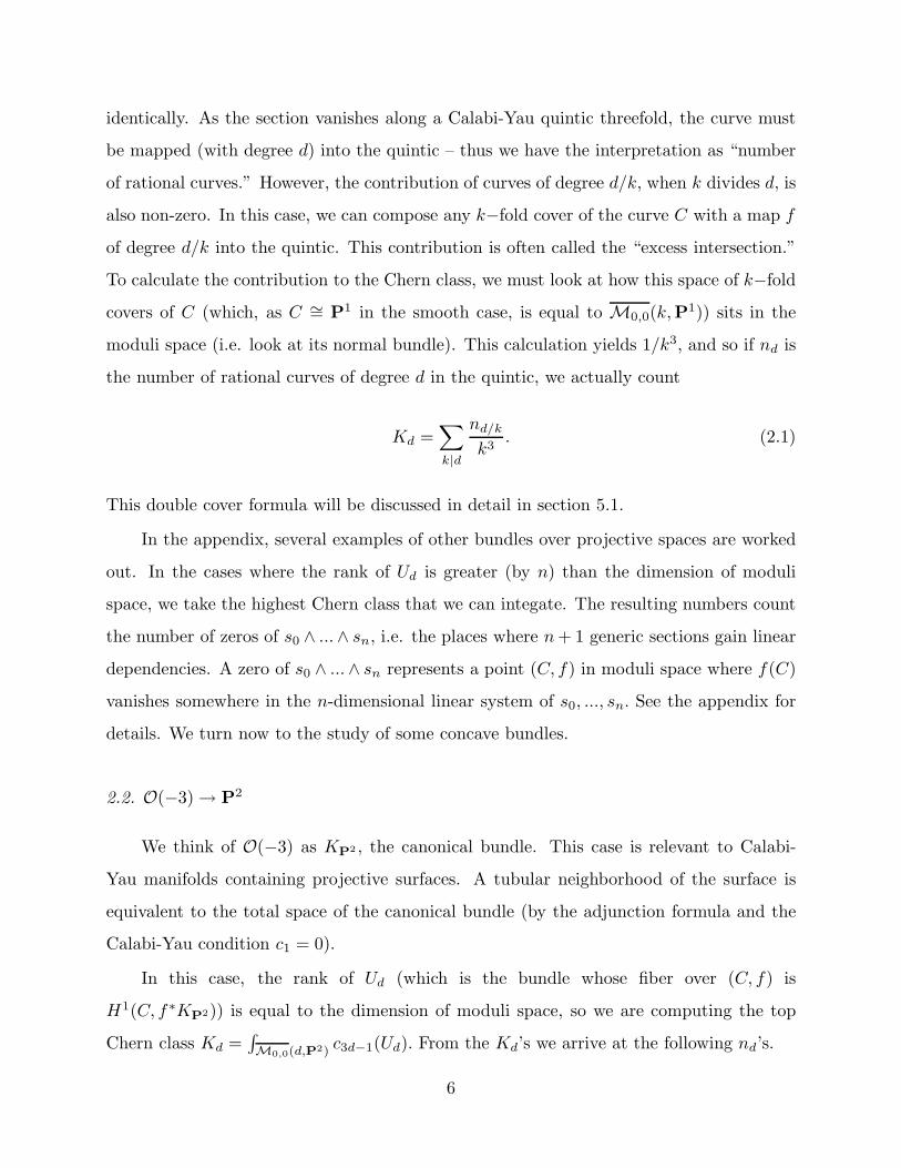
2.2. O(−3)→ P2

We think of O(−3) as KP2 , the canonical bundle. This case is relevant to Calabi-

Yau manifolds containing projective surfaces. A tubular neighborhood of the surface is

equivalent to the total space of the canonical bundle (by the adjunction formula and the

Calabi-Yau condition c1 = 0).

In this case, the rank of Ud (which is the bundle whose fiber over (C, f) is

H1(C, f∗KP2)) is equal to the dimension of moduli space, so we are computing the top

Chern class Kd =∫

M0,0(d,P2)c3d−1(Ud). From the Kd’s we arrive at the following nd’s.

6

d nd

1 3

2 −6

3 27

4 −192

5 1695

6 −17064

7 188454

8 −2228160

9 27748899

10 −360012150

Table 1: Local invariants for KP2

The interpretation for the nd’s is not as evident as for positive bundles, since no

sections of Ud can be pulled back from sections of the canonical bundle (which has no

sections). Instead, we have the following interpretation.

Suppose the P2 exists within a Calabi-Yau manifold, and we are trying to count the

number of curves in the same homology class as d times the hyperplane in P2. The analysis

for the Calabi-Yau would go along the lines of the quintic above. However, there would

necessarily be new families of zeros of your section corresponding to the families of degree

d curves in the P2 within the Calabi-Yau. These new families would be isomorphic to

M0,0(d,P2). On this space, we have to compute the contribution to the total Chern class.

To do this, we would need to use the excess intersection formula. The result (see section

5.2) is precisely given by the Kd. Let us call once again nd the integers derived from the Kd.

Suppose now that we have two Calabi-Yau’s, X0 and X1, in the same family of complex

structures, one of which (say X1 contains) a P2. Then the difference between nd(X0) and

nd(X1) should be given by the nd.

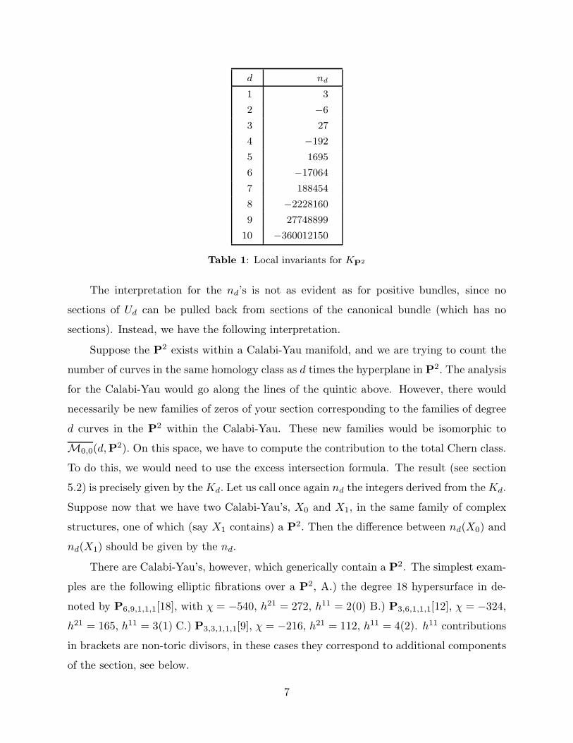
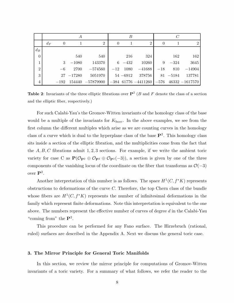
There are Calabi-Yau’s, however, which generically contain a P2. The simplest exam-

ples are the following elliptic fibrations over a P2, A.) the degree 18 hypersurface in de-

noted by P6,9,1,1,1[18], with χ = −540, h21 = 272, h11 = 2(0) B.) P3,6,1,1,1[12], χ = −324,

h21 = 165, h11 = 3(1) C.) P3,3,1,1,1[9], χ = −216, h21 = 112, h11 = 4(2). h11 contributions

in brackets are non-toric divisors, in these cases they correspond to additional components

of the section, see below.

7

A

dF 0 1 2

dB

0 540 540

1 3 −1080 143370

2 −6 2700 −574560

3 27 −17280 5051970

4 −192 154440 −57879900

B

0 1 2

216 324

6 −432 10260

−12 1080 −41688

54 −6912 378756

−384 61776 −4411260

C

0 1 2

162 162

9 −324 3645

−18 810 −14904

81 −5184 137781

−576 46332 −1617570

Table 2: Invariants of the three elliptic fibrations over P2 (B and F denote the class of a section

and the elliptic fiber, respectively.)

For such Calabi-Yau’s the Gromov-Witten invariants of the homology class of the base

would be a multiple of the invariants for Kbase. In the above examples, we see from the

first column the different multiples which arise as we are counting curves in the homology

class of a curve which is dual to the hyperplane class of the base P2. This homology class

sits inside a section of the elliptic fibration, and the multiplicities come from the fact that

the A,B,C fibrations admit 1, 2, 3 sections. For example, if we write the ambient toric

variety for case C as P(OP2 ⊕ OP2 ⊕ OP2(−3)), a section is given by one of the three

components of the vanishing locus of the coordinate on the fiber that transforms as O(−3)

over P2.

Another interpretation of this number is as follows. The space H1(C, f∗K) represents

obstructions to deformations of the curve C. Therefore, the top Chern class of the bundle

whose fibers are H1(C, f∗K) represents the number of infinitesimal deformations in the

family which represent finite deformations. Note this interpretation is equivalent to the one

above. The numbers represent the effective number of curves of degree d in the Calabi-Yau

“coming from” the P2.

This procedure can be performed for any Fano surface. The Hirzebruch (rational,

ruled) surfaces are described in the Appendix A. Next we discuss the general toric case.

3. The Mirror Principle for General Toric Manifolds

In this section, we review the mirror principle for computations of Gromov-Witten

invariants of a toric variety. For a summary of what follows, we refer the reader to the

8

start of section 2. Our treatment is somewhat more general than that of [8], as we consider

general toric varieties, though we omit some proofs which will be included in [9] .

Throughout this section, we take our target manifold to be a smooth, toric and pro-

jective manifold P. That is, we are interested in rational curves that map into P. Let us

write P as a quotient of an open affine variety:

P =CNC −∆

G,

where G ∼= (C∗)NC−M . We can write the ith action of G as

(x1, ..., xNC)→ (νqi,1x1, ..., ν

qi,NCxNC),

where ν is an arbitrary element of C∗. There is a T ≡ (S1)NC action on P induced from its

usual action on CNC . This action has NC fixed points which we denote by p1, ..., pNC. For

example, for P = P4, T is (S1)5 and the fixed points are the points with one coordinate

nonvanishing.

The T-equivariant cohomology ring can be obtained from the ordinary ring as follows.

Write the ordinary ring as a quotient

Q[B1, ..., BNC]

I,

where Bi is the divisor class of xi = 0 and I is an ideal generated by elements homogeneous

in the Bi’s. For example, for P4 we have the ring

Q[B1, ..., B5]

(B1 −B2, B1 −B3, B1 −B4, B1 −B5, B1B2B3B4B5).

Let Ji, i = 1, ...,M be the basis of nef divisors in H2(P,Z). We can write the Bl’s in terms

of the Jk’s:

Bi =∑

bijJj .

The equivariant ring is then

HT(P) =Q[κ1, ..., κM , λ1, ..., λNC

]

IT,

where IT is generated by∑

qi,jλj for i = 1, ..., NC and the nonlinear relations in I with

Bi replaced by∑

bijκj − λi. In the case of P4 this is

9

Q[κ, λ1, ..., λ5]

(∏5i=1(κ− λi),

∑

λi).

Clearly, setting λi to zero in HT(P) gives us the ordinary ring in which κj can be identified

with Jj .

Having described the base and the torus action, we also need a bundle V to define the

appropriate Gromov-Witten problem. For instance, if we are interested in rational curves

in a complete intersection of divisors in P, then V is a direct sum of the associated line

bundles. For local mirror symmetry, we can also take a concave line bundle as a component

of V . More generally, we take V = V + ⊕ V −, with V + convex and V − concave.

Before proceeding to the next section, we introduce some notation for later use. Let

Fj be the associated divisors of the line bundle summands of V , by associating each line

bundle to a divisor in the usual way. We write Fj as greater or less than zero, depending

on whether it is convex or concave. Homology classes of curves in P will be written in

the basis Hj Poincare dual to Jj . For instance, M0,0(~d;P) is the moduli space of stable

maps with image homology class∑

diHi. Finally, x denotes a formal variable for the total

Chern class.

3.1. Fixed points and a Gluing Identity

The pull-back of V to M0,1(~d;P) by the evaluation map gives a bundle of the form

ev∗(V +)⊕ ev∗(V −). Then, in terms of the forgetful map fromM0,1(~d;P) toM0,0(~d;P),

we obtain a bundle onM0,0(~d;P) ρ∗ev∗(V +)⊕R1ρ∗ev

∗(V −). The latter is the obstruction

bundle U~d.

OnM0,0(~d;P), there is a torus action induced by the action on P, i.e. by moving the

image curve under the torus action. A typical fixed point of this action is (f,P1)3, where

f(P1) is a P1 joining two T-fixed points in P.

Another type of fixed point we consider is obtained by gluing. Let (f1, C1, x1) ∈

M0,1(~r;P) and (f2, C2, x2) ∈ M0,1(~d − ~r;P) be two fixed points. Then f1(x1) is a fixed

point of P, i.e. one of the pi’s, say pk. If f2(x2) is also pk, let us glue them at the marked

points to obtain (f, C1∪C2) ∈ M0,0(~d;P), where f |C1= f1, f |C2

= f2 and f(x1 x2) = pk.

Clearly, (f, C1∪C2) is a fixed point as (f1, C1, x1) and (f2, C2, x2) are fixed points. Let us

3 We apologize for reversing notation from the previous section, and writing (f, C) instead of

(C, f). This is to agree with [8] which we closely follow in this section.

10

denote the loci of fixed points obtained by gluing as above FL(pk, ~r, ~d−~r). Over C1 ∪C2,

there is an exact sequence for V :

0→ f∗V → f∗1V ⊕ f

∗2V → V |f1(x1)=f2(x2) → 0. (3.1)

The long exact cohomology sequence then gives us a gluing identity

ΩVTcT(U~d) = cT(U~r)cT(U~d−~r), (3.2)

where ΩVT

= cT(V +)/cT(V −) is the T-equivariant Chern class of V .

This relation will generate one on the linear sigma model to which we now turn.

3.2. The spaces M~d and N~d

Because M0,0(~d;P) is a rather unwieldy space, the gluing identity we found in the

last section seems not to be useful. However, we will find, using the gluing identity, a

similar identity on a toric manifold N~d. We devote this section mainly to describing N~d

and its relation toM0,0(~d;P).

First we consider M~d ≡M0,0((1, ~d);P1×P). We will call π1 and π2 the projections to

the first and second factors of P1×P respectively. Since π2 maps to P, one might consider

a map from M~d toM0,0(~d;P) sending (f, C) to (π2f, C). However, this is not necessarily

a stable map. If it is unstable, π2 f maps some components of C to points, so if we let C′

be the curve obtained by deleting these components, there is a map π : M~d →M0,0(~d;P)

which sends (f, C) to (π2 f, C′).

Let us now recall some facts about maps from P1. A regular map to P is equivalently

a choice of generic sections of OP1(f∗Bi ·HP1), i = 1, ..., NC. For example, a map of degree

d from P1 to P4 gives five generic sections of OP1(d), i.e., five degree d polynomials. If one

takes five arbitrary sections, constrained only by being not all identically zero, one gets

a rational map instead. Generalizing this, arbitrary sections of OP1(f∗Bi · HP1) which

are not in ∆ give rational maps to P. The space N~d is the space of all such maps with

f∗(Ji) = diJP1 , where JP1 · HP1 = 1. Explicitly, we can write it as a quotient space.

Defining D =∑

djHj , we have

N~d=⊕iH

0(P1,O(Bi ·D))−∆

G. (3.3)

There is a map ψ : M~d→ N~d

, which we now describe. Take (f, C) ∈ M~dand

decompose C as a union C0∪C1 ∪ ...∪CN of not neccesarily irreducible curves, so that Cj

11

for j > 0 meets C0 at a point, and C0 is isomorphic to P1 under π1 f . Since C0∼= P1,

π2 f |C0can be regarded as a point in N[π2f(C0)], where [µ] denotes the homology class

of µ. We can also represent π2 f |Cjfor j > 0 by elements in N[π2f(Cj)], except that

since the maps are to have domain C0, in this case we take the rational map from C0 that

vanishes only at xj = Cj ∩ C0 and belongs to N[π2f(Cj)].

Having now N + 1 representatives, compose them via the map

N~r1 ⊗N~r2 → N~r1+~r2

given by multiplying sections of O(Bi). The result, since∑Ni=0[π2 f(Ci)] = D, is a point

in N~d. Thus we have obtained a map from M~d to N~d.

To illustrate, let us take the case of P4 again. Here (f, C) is a degree (1, d) map.

Let us decompose C as before into C0 ∪ ... ∪ CN , with xi = Ci ∩ C0 and π1 f |C0an

isomorphism. The image of ψ is a rational morphism given as a map by π2 f |C0except

at the points xi. At xi, a generic hyperplane of P4 pulled back vanishes to the order given

by the multiplicity of [π2 f(Ci)] in terms of a generator.

So far we have discussed the spaces and the maps between them. We now briefly

describe the torus actions they admit. Clearly, M~d has an S1 ×T action induced from an

action on P1 ×P. In suitable coordinates, the S1 action is [w0, w1]→ [eαw0, w1].

Since sections of OP1(1) is also a one-dimensional projective space, there is an S1

action on H0(P1,OP1(1)). This induces an action on sections of OP1(d). N~d is defined

by the latter, so it admits an S1 action. In addition, it has a T-action induced from the

action on O(Bi).

The map π is obviously T-equivariant, since the T-actions are induced from P. It is

shown in [9] that ψ is (S1 ×T)-equivariant. Summarizing, we have the following maps:

N~d

π

←−M~d

ψ

−→M0,0(~d;P)ρ

←−M0,1(~d;P)ev

−→P.

Pushing and pulling our problem to N~d, we define

Q~d = ψ!π∗cT(U~d).

12

3.3. Euler data

In this section we will derive from the gluing identity a simpler identity on N~d. Recall

that the gluing identity holds over fixed loci FL(pi, ~r, ~d− ~r) ∈ M0,0(~d;P). Therefore, an

identity holds over π−1(FL(pi, ~r, ~d − ~r)) in M~d under pull-back by π. We next turn to

describing a sublocus of π−1(FL(pi, ~r, ~d− ~r)) which, as we will see later is mapped by ψ

to a fixed point in N~d.

Let Fpi,~r denote the fixed point loci inM0,1(~r;P) with the marked point mapped to

pi. Let (f1, C1, x1) ∈ Fpi,~r and (f2, C2, x2) ∈ Fpi,~d−~rbe two points. We define a point

(f, C) in M~d as follows. For C we take (C0 ≡ P1) ∪ C1 ∪ C2, with C0 ∩ C1 = x1 and

C0 ∩C2 = x2. For the map f , we define it by giving the projections π1 f and π2 f . We

require π1 f(C1) = 0, π1 f(C2) = ∞ and π1 f |C0be an isomorphism. This “fixes”

π1f , since any other choice is related by an automorphism of the domain curve preserving

x1 and x2, which is irrelevant in M~d. We require π2 f to map C1 as f1, C2 as f2 and C0

to f1(x1). Clearly, π maps (f, C) to a point in FL(pi, ~r, ~d− ~r). Let us denote the loci of

such (f, C)’s by MFL(pi, ~r, ~d− ~r). By construction, it is isomorphic to Fpi,~r × Fpi,~d−~r.

We verify (f, C) is a fixed point. fi(Ci) and pi are fixed in P, so f is T-fixed. The

S1-action fixes only 0 and∞ on the first factor of P1×P. Nevertheless, the point (f, C0∪

C1 ∪ C2) remains fixed under the S1 action, as we need to divide out by automorphisms

of C0 preserving x1 and x2.

We now compare the maps just constructed with the fixed points of N~d. It will be

most convenient to do so by describing the latter in terms of rational morphisms. So take

a point in N~d, viewed as a rational morphism from C0 ≡ P1. Let x1, ..., xN be the points

where it is undefined. At xi, the chosen sections of O(Bj · D) vanish to certain orders,

including possibly zero. A generic section of O(Jj ·D) = O(dj) vanishes to order, say rj

at x1. Any section of a line bundle O(L) pulled back by the map then vanishes at x1 at

least to order L ·∑

rjHj .

Therefore the rational morphism is equivalent to the data of a regular map from C0

and a curve class for each bad point. The classes for the bad points indicate the multiplicity

of vanishing of a generic section of a pulled-back line bundle. Altogether, the class of the

image of the regular map and the curve classes we associate to the bad points sum to D,

since a generic section of O(L) must have exactly L ·D zeroes.

Now we can deduce the fixed points of N~d. The T-action moves the image of a rational

morphism, whereas the S1 action rotates the domain P1 about an axis joining 0 and ∞.

13

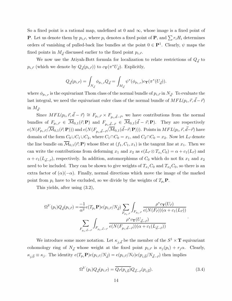
So a fixed point is a rational map, undefined at 0 and ∞, whose image is a fixed point of

P. Let us denote them by pi,~r, where pi denotes a fixed point of P, and∑

riHi determines

orders of vanishing of pulled-back line bundles at the point 0 ∈ P1. Clearly, ψ maps the

fixed points in M~d discussed earlier to the fixed point pi,~r.

We now use the Atiyah-Bott formula for localization to relate restrictions of Q~d to

pi,~r (which we denote by Q~d(pi,~r)) to cT(π∗U~d). Explicitly,

Q~d(pi,~r) =

∫

N~d

φpi,~rQ~d =

∫

M~d

ψ∗(φpi,~r)cT(π∗(U~d)).

where φpi,~ris the equivariant Thom class of the normal bundle of pi,~r inN~d. To evaluate the

last integral, we need the equivariant euler class of the normal bundle of MFL(pi, ~r, ~d−~r)

in M~d.

Since MFL(pi, ~r, ~d − ~r) ∼= Fpi,~r × Fpi,~d−~r, we have contributions from the normal

bundles of Fpi,~r ∈ M0,1(~r;P) and Fpi,~d−~r∈ M0,1(~d − ~r;P). They are respectively

e(N(Fpi,~r/M0,1(~r;P))) and e(N(Fpi,~d−~r/M0,1(~d−~r;P))). Points inMFL(pi, ~r, ~d−~r) have

domain of the form C0∪C1∪C2, where C1∩C0 = x1, and C2∩C0 = x2. Now let L~r denote

the line bundle onM0,1(~r;P) whose fiber at (f1, C1, x1) is the tangent line at x1. Then we

can write the contributions from deforming x1 and x2 as e(L~r ⊗ Tx1C0) = α+ c1(L~r) and

α+ c1(L~d−~r), respectively. In addition, automorphisms of C0 which do not fix x1 and x2

need to be included. They can be shown to give weights of Tx1C0 and Tx2

C0, so there is an

extra factor of (α)(−α). Finally, normal directions which move the image of the marked

point from pi have to be excluded, so we divide by the weights of TpiP.

This yields, after using (3.2),

ΩV (pi)Q~d(pi,~r) =−1

α2e(Tpi

P)e(pi,~r/N~d)∑

Fpi,~r

∫

Fpi,~r

ρ∗cT(U~r)

e(N(F~r))(α+ c1(L~r))

∑

Fpi,~d−~r

∫

Fpi,~d−~r

ρ∗cT(U~d−~r)

e(N(Fpi,~d−~r))(α+ c1(L~d−~r))

.

We introduce some more notation. Let κj,~d be the member of the S1 ×T equivariant

cohomology ring of N~d whose weight at the fixed point pi,~r is κj(pi) + rjα. Clearly,

κj,~0 ≡ κj . The identity e(TpiP)e(pi,~r/N~d) = e(pi,~r/N~r)e(pi,~0/N~d−~r) then implies

ΩV (pi)Q~d(pi,~r) = Q~r(pi,~0)Q~d−~r(pi,~0). (3.4)

14

Here the overbar is an automorphism of the S1 × T equivariant cohomology ring with

α = −α and κj,~d = κj,~d. A sequence of equivariant cohomology classes satisfying (3.4) is

called in [8] a set of ΩV -Euler data.

3.4. Linked Euler data

If we knew the values of Q~dat all fixed points, we would also know Q~d

as a class.

Since we do not know this, we will use equivariance to compute Q~d at certain points, for

example, those that correspond to the T-invariant P1’s in P. It turns out that this is also

sufficient, as we will find Euler data which agree with Q~dat those points, and a suitable

comparison between the two gives us the rest.

Before we begin the computation, we first describe a T-equivariant map from N~0 = P

to N~d. Sections of O(Bi ·D) over P1 are polynomials in w0 and w1, where w0 and w1 are

as before coordinates so that the S1 action takes the form [w0, w1] → [eαw0, w1]. Each

polynomial contains a unique monomial invariant under the S1 action. By sending the

coordinates of a point to the coefficients of the invariant monomials, we hence obtain a

map I~d from N~0 to N~d.

We begin with the case of a convex line bundle O(L), where L denotes the associated

divisor. Let (f,P1) be a point inM0,0(~d;P) with f(P1) being a multiple of the T-invariant

P1 joining pi and pj in P. The fiber of the obstruction bundle at (f,P1) is H0(O(L ·D)),

which is spanned in appropriate coordinates for the P1 by uk0uL·D−k1 , k = 0, ..., L ·D.

Choose a basis so that u1 = 0 is mapped to pi, and u0 = 0 mapped to pj . Since the

section uL·D0 does not vanish at u1 = 0, its weight is equal to the weight of L at pi, which

we denote by L(pi). Similarly, uL·D1 has weight L(pj). Hence the induced weight on u1/u0

is (L(pj)− L(pi))/(L ·D), giving us the weights of all sections.

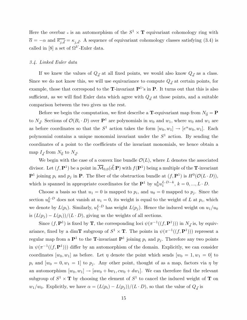
Since (f,P1) is fixed by T, the corresponding loci ψ(π−1((f,P1))) in N~d is, by equiv-

ariance, fixed by a dimT subgroup of S1 ×T. The points in ψ(π−1((f,P1))) represent a

regular map from a P1 to the T-invariant P1 joining pi and pj . Therefore any two points

in ψ(π−1((f,P1))) differ by an automorphism of the domain. Explicitly, we can consider

coordinates [w0, w1] as before. Let η denote the point which sends [w0 = 1, w1 = 0] to

pi and [w0 = 0, w1 = 1] to pj . Any other point, thought of as a map, factors via η by

an automorphism [w0, w1] → [aw0 + bw1, cw0 + dw1]. We can therefore find the relevant

subgroup of S1 × T by choosing the element of S1 to cancel the induced weight of T on

w1/w0. Explicitly, we have α = (L(pi)− L(pj))/(L ·D), so that the value of Q~d is

15

∏

k

(x+ L(pj) + kα).

The weight of κi,~d under (S1 × T)/(α − (L(pi) − L(pj))/(L · D)) at any point in

ψ(π−1((f,P1))) is the same as its weight under T at the corresponding point obtained

by setting w0 to zero. For η, setting w0 to zero gives a point in N~d which can be thought

of as a rational map to pj . Since I~d is equivariant, the weight of κi,~d

at this point is the

same as the weight of κi at pj . Thus, as∑

liκi(pj) = L(pj), the value of Q~d is the same

as the value of P~d, where P~d is given by

∏

k

(x+∑

liκi,~d + kα).

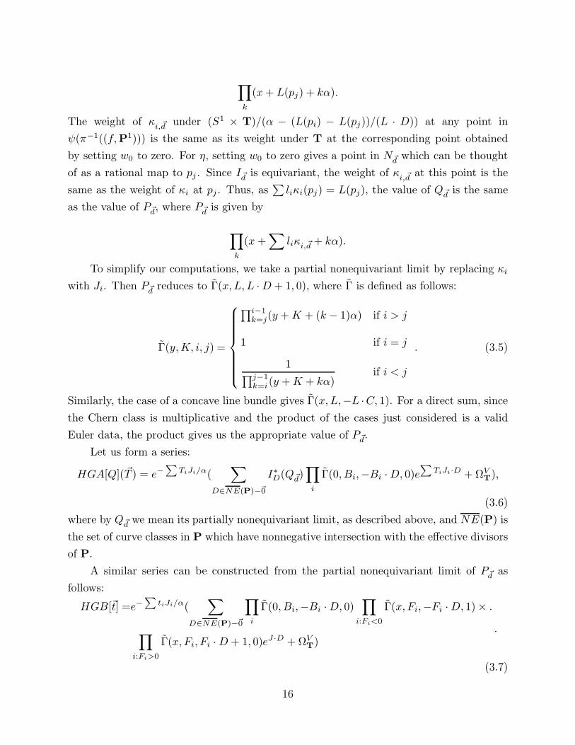
To simplify our computations, we take a partial nonequivariant limit by replacing κi

with Ji. Then P~d reduces to Γ(x, L, L ·D + 1, 0), where Γ is defined as follows:

Γ(y,K, i, j) =

∏i−1k=j(y +K + (k − 1)α) if i > j

1 if i = j

1∏j−1k=i(y +K + kα)

if i < j

. (3.5)

Similarly, the case of a concave line bundle gives Γ(x, L,−L ·C, 1). For a direct sum, since

the Chern class is multiplicative and the product of the cases just considered is a valid

Euler data, the product gives us the appropriate value of P~d.

Let us form a series:

HGA[Q](~T ) = e−∑

TiJi/α(∑

D∈NE(P)−~0

I∗D(Q~d)∏

i

Γ(0, Bi,−Bi ·D, 0)e∑

TiJi·D + ΩVT

),

(3.6)

where by Q~dwe mean its partially nonequivariant limit, as described above, and NE(P) is

the set of curve classes in P which have nonnegative intersection with the effective divisors

of P.

A similar series can be constructed from the partial nonequivariant limit of P~d as

follows:

HGB[~t] =e−∑

tiJi/α(∑

D∈NE(P)−~0

∏

i

Γ(0, Bi,−Bi ·D, 0)∏

i:Fi<0

Γ(x, Fi,−Fi ·D, 1)× .

∏

i:Fi>0

Γ(x, Fi, Fi ·D + 1, 0)eJ·D + ΩVT

).

(3.7)

16

If we take the example of the quintic in P4, dimH2(P,Z) = 1, so we have

HGB[t] = e−J/α(∑

d>0

∏5dm=1(x+ 5H −mα)

∏dm=1(x+H −mα)

5 + 5H). (3.8)

For local mirror symmetry, we can take V = KP2 , giving

HGB[t] = e−J/α(∑

d>0

∏3d−1m=1 (x− 3H +mα)

∏dm=1(x+H −mα)

3 −1

3H). (3.9)

To compare HGB[~t] and HGA[~T ], let us expand HGB[~t] at large α, keeping terms

to order 1/α. It is shown in [9] that HGA[~T ] has the form ΩVT

(1− (∑

TiJi)/α). Equating

the two expressions gives us ~T in terms of ~t. Then setting HGA[~T (~t)] = HGB[~t] gives us

QD as a function of Ji and α, from which we may obtain KD [9]:

(2−∑

diti)KD

α3=

∫

P

e−∑

tiJi/αQ~d

∏

j

Γ(0, Bj,−Bj ·D, 0). (3.10)

4. Explicit Verification Through Fixed-Point Methods

4.1. Some examples

Though the techniques of section one are extremely powerful, it is often satisfying –

and a good check of one’s methods – to do some computations by hand. In this section,

we outline fixed point techniques for doing so, and walk through several examples. In this

way, we have verified many of the results in the appendices for low degrees (d = 1, 2, 3).

Readers familiar with such exercises may wish to skip to the next subsection.

All the bundles described in section two are equivariant with respect to the torus

T -action which acts naturally on the toric manifold P. Let t ∈ T be a group element

acting on P. Then if (C, f, ∗) ∈ M0,1(~d;P) and (C, f) ∈ M0,0(~d;P) the induced torus

action sends theses points to (C, t f, ∗) and (C, t f), respectively. The bundle actions

are induced by the natural T -action on the canonical bundle, K.

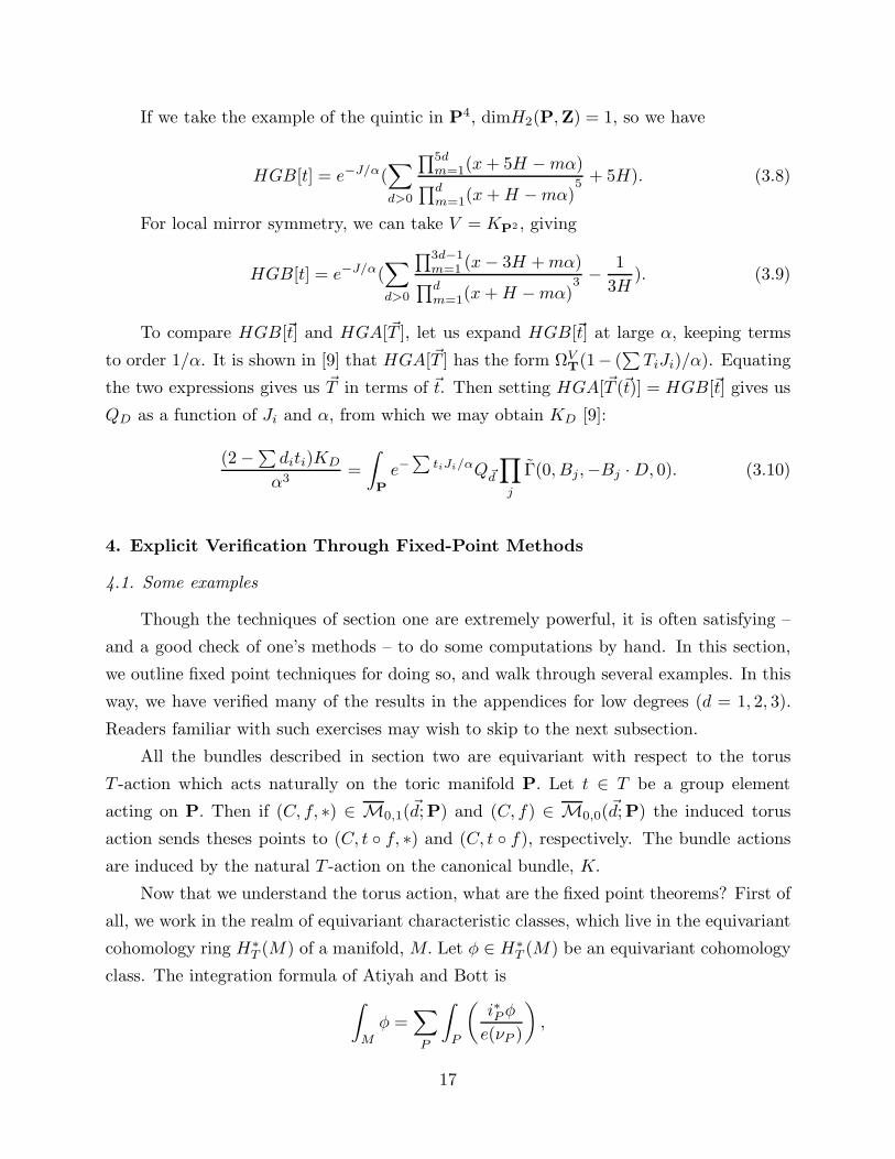
Now that we understand the torus action, what are the fixed point theorems? First of

all, we work in the realm of equivariant characteristic classes, which live in the equivariant

cohomology ring H∗T (M) of a manifold, M. Let φ ∈ H∗

T (M) be an equivariant cohomology

class. The integration formula of Atiyah and Bott is

∫

M

φ =∑

P

∫

P

(

i∗Pφ

e(νP )

)

,

17

where the sum is over fixed point sets P, iP is the embedding in M, and e(νP ) is the Euler

class of the normal bundle νP along P. For P consisting of isolated points and φ the Chern

class (determinant), we get the ratio of the product of the weights of the T -action on the

fibers at P (numerator) over the product of the weights of the T -action on the tangent

bundle to M at P (denominator). One needs only to determine the fiber and tangent

bundle at P and figure out the weights.

Let’s start with degree one (K1) for the quintic (O(5) → P4). Let Xi 7→ αλi

i Xi,

i = 1, ..., 5, be the (C∗)5 action on C5 (P4 = P(C5)), where ~α ∈ (C∗)5 and the λi are the

weights. The fixed curves are Pij , where i, j run from 1 to 5 : Pij = Xk = 0, k 6= i, j.

Since f is a degree one map, we may equate C ∼= f(C) and the pull-back of O(5) is

therefore equal to O(5) on Ce. Recall the bundle O(5) on P1. Its global sections are

degree five polynomials in the homogeneous coordinates [X, Y ], so a convenient basis is

XaY 5−a, a = 0, ..., 5 (or ua in a local coordinate u = X/Y ). The weights of these

sections are aµ+ (5− a)ν, if µ and ν are the weights of the torus (C∗)2 action on C2. The

map f : Ce → P4 looks like [X, Y ] 7→ [..., X, ..., Y, ...] with non-zero entries only in the ith

and jth positions. Therefore, the weights of U1 at the fixed point (C, f) are aλi+(5−a)λj ,

a = 0...5. To take the top Chern class we take the product of these six weights.

We have to divide this product by the product of the weights of the normal bundle,

which in this case (the image f(C) is smooth) are the weights of H0(C, f∗N), where N

is the normal bundle to f(C). More generally, we take sections of the pull-back of TP4

and remove sections of TC . The normal bundle of Pij is equal to O(1) ⊕ O(1) ⊕ O(1),

each corresponding to a direction normal to f(C) and each of which has two sections. Let

w = Xj/Xi be a coordinate along C ∼= Pij on the patch Xi 6= 0. If zk = Xk/Xi is a local

coordinate of P4, then delk ≡∂∂zk

is a normal vector field on C with weight λk − λi. w∂k

is the other normal vector field corresponding to the direction k, and has weight λk − λj .

Summing over the

(

52

)

= 20 choices of image curve Pij gives us

K1 =∑

(ij)

∏5a=0[aλi + (5− a)λj ]

∏

k 6=i,j(λk − λi)(λk − λj)= 2875,

the familiar result.

Let’s try degree two (K2) for KP2 . The dimension of M0,0(d;P2) is 3d − 1 = 5 for

d = 2. What are the fixed points? Well, the image of (C, f) must an invariant curve, so

there are two choices for degree two. Either the image is a smooth P1 or the union of two

18

P1’s. There are three fixed points on P2 and therefore

(

32

)

= 3 invariant Pij ’s. If the

image is a smooth P1, the domain curve may either be a smooth P1, in which case the

map is a double cover (let’s call this case 1a), or it may have two component P1’s joined

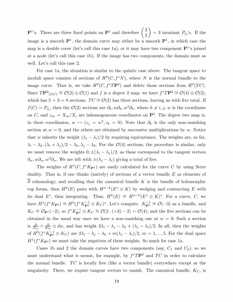
at a node (let’s call this case 1b). If the image has two components, the domain must as

well. Let’s call this case 2.

For case 1a, the situation is similar to the quintic case above. The tangent space to

moduli space consists of sections of H0(C, f∗N), where N is the normal bundle to the

image curve. That is, we take H0(C, f∗TP2) and delete those sections from H0(TC).

Since TP2|f(C)∼= O(2)⊕O(1) and f is a degree 2 map, we have f∗TP2 ∼= O(4)⊕O(2),

which has 5 + 3 = 8 sections. TC ∼= O(2) has three sections, leaving us with five total. If

f(C) = Pij , then the O(2) sections are ∂k, w∂k, w2∂k, where k 6= i, j, w is the coordinate

on C, and zm = Xm/Xi are inhomogeneous coordinates on P2. The degree two map is,

in these coordinates, w 7→ (zj = w2, zk = 0). Note that ∂k is the only non-vanishing

section at w = 0, and the others are obtained by successive multiplications by w. Notice

that w inherits the weight (λj − λi)/2 by requiring equivariance. The weights are, so far,

λi − λk, (λi + λj)/2 − λk, λj − λk. For the O(4) sections, the procedure is similar, only

we must remove the weights 0,±(λi − λj)/2, as these correspond to the tangent vectors

∂w, w∂w, w2∂w. We are left with ±(λj − λi) giving a total of five.

The weights of H1(C, f∗KP2) are easily calculated for the curve C by using Serre

duality. That is, if one thinks (naively) of sections of a vector bundle E as elements of

∂ cohomology, and recalling that the canonical bundle K is the bundle of holomorphic

top forms, then Hk(E) pairs with Hn−k(E∗ ⊗ K) by wedging and contracting E with

its dual E∗, then integrating. Thus, Hk(E) ∼= Hn−k(E∗ ⊗ K)∗. For a curve, C, we

have H1(f∗KP2) ∼= H0(f∗K−1P2 ⊗KC)∗. Let’s compute. K−1

P2∼= O(−3) as a bundle, and

KC∼= OP1(−2), so f∗K−1

P2 ⊗KC∼= O(2 · (+3) − 2) = O(4), and the five sections can be

obtained in the usual way once we have a non-vanishing one at w = 0. Such a section

is ∂∂zj∧ ∂∂zk⊗ dw, and has weight 2λi − λj − λk + (λj − λi)/2. In all, then the weights

of H0(f∗K−1P2 ⊗ KC) are 2λi − λj − λk +m(λj − λi)/2, m = 1, ..., 5. For the dual space

H1(f∗KP2) we must take the negatives of these weights. So much for case 1a.

Cases 1b and 2 the domain curves have two components (say, C1 and C2), so we

must understand what is meant, for example, by f∗TP2 and TC in order to calculate

the normal bundle. TC is locally free (like a vector bundle) everywhere except at the

singularity. There, we require tangent vectors to vanish. The canonical bundle, KC , is

19

defined as a line bundle of holomorphic differentials, with the following construction at the

singularity. Let f(w)dw be a differential along C1, and let g(z)dz be a differential along C2

where the singularity is taken to be (z = 0) ∼ (w = 0). To define a differential along the

total space, we allow f and g to have up to simple poles at the origin, with the requirement

that the total residue vanish: reswf+reszg = 0.What this does is serve as an identification,

at the singularity, of the fibers of the canonical bundles of the two components. In this

way, we arrive at a line ”bundle.” This canonical bundle, when restricted to a component

Ci, looks like KCi(p), where the “(p)” indicates twisting by the point, i.e. allowing poles.

At this point, we can proceed with the calculation. Consider case 2, for which the

map f is a bijection. The sections of H1(f∗KP2) ∼= H0(f∗(KP2) can be looked at on each

component, where KC |Ciis as above. Hence on Ci we have

1

w

∂

∂z1∧

∂

∂z2⊗ dw, 1

∂

∂z1∧

∂

∂z2⊗ dw, w

∂

∂z1∧

∂

∂z2⊗ dw.

On the the other component, we have three analogous sections, but two with poles need

to be identified, since they are related by the requirement of no total residue. Indeed, this

identification is compatible with equivariance, since 1wdw has zero weight. All in all, we

have weights (recalling duality) λj + λk − 2λi, λk − λi, λk − λj , λj − λi, λj − λk.

The normal bundle to moduli space consists of sections of the pull-back of tangent

vectors on P2, less global tangent vectors on C. In addition, we include TpC1⊗TpC2, which

is a factor corresponding to a normal direction in which the node is resolved [6] . Since the

maps from components are degree one for these cases, we can take as sections of the normal

bundles (two each) ∂w, z∂w and ∂z, w∂z. Here we have identified the coordinate of the other

component with the coordinate of P2 normal to the component. The TpC1 ⊗ TpC2 piece

gives ∂w ⊗ ∂z. In total, the weights are λi − λj , λk − λj , λi − λk, λj − λk, 2λi − λj − λk.

One checks that the product of the numerator weights divided by the denominator

weights is equal to −1. Since there are three graphs of this type, the total contribution to

K2 is −3. Graphs whose image is a single fixed P1 contribute −21/8,4 giving K2 = −45/8.

In physics, local mirror symmetry is all that is needed to describe the effective quantum

field theory from compactification on a Calabi-Yau manifold which contains a holomor-

phic surface, if we take an appropriate limit. In this limit, the global structure of the

4 Because we are considering integrals in the sense of orbifolds, we must divide out the con-

tribution of each graph by the order of the automorphism group of the map. Automorphisms are

maps γ : C → C such that f γ = f. Cases 1a and 1b have Z2 automorphism groups.

20

Calabi-Yau manifold becomes irrelevant (hence the term “local”), and we can learn about

the field theory by studying the local geometry of the surface – its canonical bundle. We

can therefore construct appropriate surfaces to study aspects of four-dimensional gauge

theories of our choosing [3] . The growth of the Gromov-Witten invariants (or their local

construction) in a specified degree over the base P1 is related to the Seiberg-Witten co-

efficient at that degree in the instanton expansion of the holomorphic prepotential of the

gauge theory. For example, the holomorphic vanishing cycles of an An singularity fibered

over a P1 give SU(n+ 1) gauge theory (the McKay correspondence, essentially), and one

can construct a Calabi-Yau manifold containing this geometry to check this [3] [2]. In this

case, the local surface is singular, as it is several intersecting P1’s fibered over a P1 (for

A1 we can take two Hirzebruch surfaces intersecting in a common section. For this reason,

it is important to understand the case where the surface is singular, as well. We will have

more to say about this in section six.

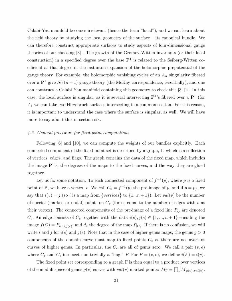
4.2. General procedure for fixed-point computations

Following [6] and [10], we can compute the weights of our bundles explicitly. Each

connected component of the fixed point set is described by a graph, Γ, which is a collection

of vertices, edges, and flags. The graph contains the data of the fixed map, which includes

the image P1’s, the degrees of the maps to the fixed curves, and the way they are glued

together.

Let us fix some notation. To each connected component of f−1(p), where p is a fixed

point of P, we have a vertex, v. We call Cv = f−1(p) the pre-image of p, and if p = pj , we

say that i(v) = j (so i is a map from vertices to 1...n+ 1). Let val(v) be the number

of special (marked or nodal) points on Cv (for us equal to the number of edges with v as

their vertex). The connected components of the pre-image of a fixed line Pij are denoted

Ce. An edge consists of Ce together with the data i(e), j(e) ∈ 1, ..., n+ 1 encoding the

image f(C) = Pi(e),j(e), and de the degree of the map f |Ce. If there is no confusion, we will

write i and j for i(e) and j(e). Note that in the case of higher genus maps, the genus g > 0

components of the domain curve must map to fixed points Cv as there are no invariant

curves of higher genus. In particular, the Ce are all of genus zero. We call a pair (v, e)

where Cv and Ce intersect non-trivially a “flag,” F. For F = (v, e), we define i(F ) = i(v).

The fixed point set corresponding to a graph Γ is then equal to a product over vertices

of the moduli space of genus g(v) curves with val(v) marked points: MΓ =∏

vMg(v),val(v).

21

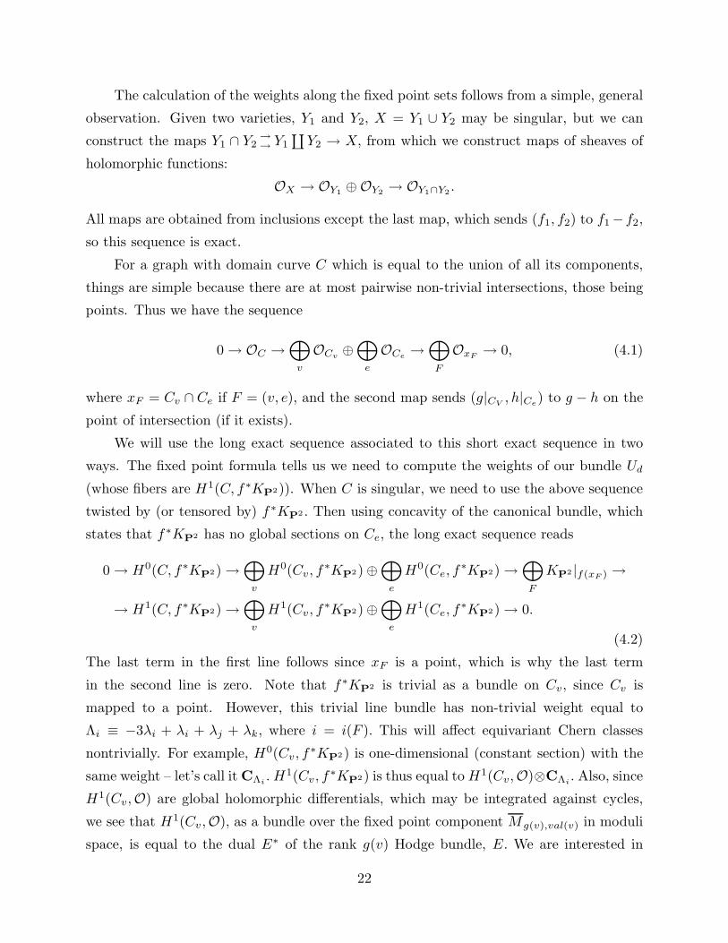
The calculation of the weights along the fixed point sets follows from a simple, general

observation. Given two varieties, Y1 and Y2, X = Y1 ∪ Y2 may be singular, but we can

construct the maps Y1 ∩ Y2→→ Y1

∐

Y2 → X, from which we construct maps of sheaves of

holomorphic functions:

OX → OY1⊕OY2

→ OY1∩Y2.

All maps are obtained from inclusions except the last map, which sends (f1, f2) to f1−f2,

so this sequence is exact.

For a graph with domain curve C which is equal to the union of all its components,

things are simple because there are at most pairwise non-trivial intersections, those being

points. Thus we have the sequence

0→ OC →⊕

v

OCv⊕

⊕

e

OCe→

⊕

F

OxF→ 0, (4.1)

where xF = Cv ∩ Ce if F = (v, e), and the second map sends (g|CV, h|Ce

) to g − h on the

point of intersection (if it exists).

We will use the long exact sequence associated to this short exact sequence in two

ways. The fixed point formula tells us we need to compute the weights of our bundle Ud

(whose fibers are H1(C, f∗KP2)). When C is singular, we need to use the above sequence

twisted by (or tensored by) f∗KP2 . Then using concavity of the canonical bundle, which

states that f∗KP2 has no global sections on Ce, the long exact sequence reads

0→ H0(C, f∗KP2)→⊕

v

H0(Cv, f∗KP2)⊕

⊕

e

H0(Ce, f∗KP2)→

⊕

F

KP2 |f(xF ) →

→ H1(C, f∗KP2)→⊕

v

H1(Cv, f∗KP2)⊕

⊕

e

H1(Ce, f∗KP2)→ 0.

(4.2)

The last term in the first line follows since xF is a point, which is why the last term

in the second line is zero. Note that f∗KP2 is trivial as a bundle on Cv, since Cv is

mapped to a point. However, this trivial line bundle has non-trivial weight equal to

Λi ≡ −3λi + λi + λj + λk, where i = i(F ). This will affect equivariant Chern classes

nontrivially. For example, H0(Cv, f∗KP2) is one-dimensional (constant section) with the

same weight – let’s call it CΛi. H1(Cv, f

∗KP2) is thus equal toH1(Cv,O)⊗CΛi. Also, since

H1(Cv,O) are global holomorphic differentials, which may be integrated against cycles,

we see that H1(Cv,O), as a bundle over the fixed point component Mg(v),val(v) in moduli

space, is equal to the dual E∗ of the rank g(v) Hodge bundle, E. We are interested in

22

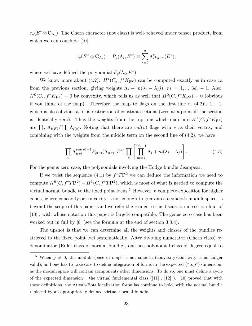
cg(E∗⊗CΛi

). The Chern character (not class) is well-behaved under tensor product, from

which we can conclude [10]

cg(E∗ ⊗CΛi

) = Pg(Λi, E∗) ≡

g∑

r=0

Λri cg−r(E∗),

where we have defined the polynomial Pg(Λi, E∗)

We know more about (4.2). H1(Ce, f∗KP2) can be computed exactly as in case 1a

from the previous section, giving weights Λi + m(λi − λ)j), m = 1, ..., 3de − 1. Also,

H0(Ce, f∗KP2) = 0 by convexity, which tells us as well that H0(C, f∗KP2) = 0 (obvious

if you think of the map). Therefore the map to flags on the first line of (4.2)is 1 − 1,

which is also obvious as it is restriction of constant sections (zero at a point iff the section

is identically zero). Thus the weights from the top line which map into H1(C, f∗KP2)

are∏

F Λi(F )/∏

v Λi(v). Noting that there are val(v) flags with v as their vertex, and

combining with the weights from the middle term on the second line of (4.2), we have

∏

v

Λval(v)−1i(v) Pg(v)(Λi(v), E

∗)∏

e

[

3de−1∏

m=1

Λi +m(λi − λj)

]

. (4.3)

For the genus zero case, the polynomials involving the Hodge bundle disappear.

If we twist the sequence (4.1) by f∗TP2 we can deduce the information we need to

compute H0(C, f∗TP2)−H1(C, f∗TP2), which is most of what is needed to compute the

virtual normal bundle to the fixed point locus.5 However, a complete exposition for higher

genus, where concavity or convexity is not enough to guarantee a smooth moduli space, is

beyond the scope of this paper, and we refer the reader to the discussion in section four of

[10] , with whose notation this paper is largely compatible. The genus zero case has been

worked out in full by [6] (see the formula at the end of section 3.3.4).

The upshot is that we can determine all the weights and classes of the bundles re-

stricted to the fixed point loci systematically. After dividing numerator (Chern class) by

denominator (Euler class of normal bundle), one has polynomial class of degree equal to

5 When g 6= 0, the moduli space of maps is not smooth (convexity/concavity is no longer

valid), and one has to take care to define integration of forms in the expected (“top”) dimension,

as the moduli space will contain components other dimensions. To do so, one must define a cycle

of the expected dimension – the virtual fundamental class ([11] , [12] ). [10] proved that with

these definitions, the Atiyah-Bott localization formulas continue to hold, with the normal bundle

replaced by an appropriately defined virtual normal bundle.

23

the dimension of the fixed locus. What’s left is to integrate these classes over the moduli

spaces of curves (not maps) Mg(v),val(v) at each vertex. These integrals obey famous re-

cursion relations [13], which entirely determine them. A program for doing just this has

been written by [14] . With this, and an algorithm for summing over graphs (with ap-

propriate symmetry factors), one can completely automate the calculation of higher genus

Gromov-Witten invariants. Subtleties remain, however, regarding multicovers [15], [16],

[17] .

5. Virtual Classes and the Excess Intersection Formula

One of the foundations of the theory of the moduli space of maps has been the con-

struction of the virtual class [12] [11] . A given space of maps M(β,X) may be of the

wrong dimension, and the virtual class provides a way to correct for this. We consider

the “correct dimension” to be one imposed either by physical theory, or by the require-

ment that the essential behavior of the moduli space be invariant under deformations of

X (this may include topological deformations of X , or just deformations of symplectic or

almost complex structures). The virtual class is a class in the cohomology (or Chow) ring

of M(β,X); its principal properties are that it is a class in the cohomology ring of the

expected dimension, and that numbers calculated by integrating over the virtual class are

invariant under deformations of X . See [12] [11] for more exact and accurate statements.

One main theme of this paper is to use the invariance under deformation to either calculate

these numbers, or to explain the significance of a calculation.

The idea of a cohomology class (or cohomology calculation) which corrects for “im-

proper behavior” has been around for a long time in intersection theory. One example is

the excess intersection formula. If we attempt to intersect various classes in a cohomology

ring, and if we choose representatives of those classes which fail to intersect transversely,

the resulting dimension of the intersection may be too large. The excess intersection for-

mula allows us to perform a further calculation on this locus to determine the actual class

of the intersection. The purpose of this section is to describe the excess intersection for-

mula for degeneracy loci of vector bundles, and to use this formula to evaluate or explain

some mirror symmetry computations. In the cases we examine, the moduli space of maps

to our space X can be given as the degeneracy locus of a vector bundle on a larger space

of maps. In each case that these degeneracy loci are of dimension larger than expected,

24

the virtual class will turn out to be the same as the construction given by the excess in-

tersection formula. The virtual class and the excess intersection formula are both aspects

of the single idea mentioned above, and have as common element in their construction the

notion of the refined intersection class [18].

To a vector bundle E of rank r on a smooth algebraic variety X of dimension n, we

associate the Chern classes, cj(E), j = 0, . . . , r, and also the total Chern class c(E) =

1 + c1(E) + c2(E) + · · ·+ cr(E). These classes are elements of the cohomology ring of X .

The class cj(E) represents a class of codimension j in X , and in particular the class cn(E)

is a class in codimension n, and can be associated with a number. For any class α in the

ring, the symbol∫

Xα means to throw away all parts of α except those parts in degree n,

and evaluate the number associated to those parts.

For a vector bundle E whose rank is greater or equal to the dimension n of X , we are

often interested in calculating the number associated to cn(E), or in the previous notation,∫

Xc(E). One way to compute Chern classes is to realize them as degeneracy loci of linear

combinations of sections. If E is of rank r ≥ n, and we take r−n+1 generic global sections

σ1, . . . , σr−n+1, the locus of points where σ1, . . . , σr−n+1 fail to be linearly independent

represents the class cn(E). Often this way of interpreting the Chern classes is the one

which has the most geometric meaning. The statement “generic” above means that if we

carry out this procedure and find out that the degeneracy locus is of the correct dimension

(that is: points), then the sections were generic enough.

Sometimes the sections we can get our hands on to try and calculate∫

Xc(E) with

are not generic in this sense, and the degeneracy locus consists of some components which

are positive dimensional. In this situation, the excess intersection formula tells us how

to associate to each positive dimensional connected component of the degeneracy locus a

number, called the “excess intersection contribution”. This number is the number of points

which the component “morally” accounts for. Part of the excess intersection theorem is

the assertion that the sum of the excess intersection contributions over all the connected

components of the degeneracy locus, and the sum of the remaining isolated points add

up to∫

Xc(E). This corresponds to the invariance of numbers computed using the virtual

class under deformations of the target manifold.

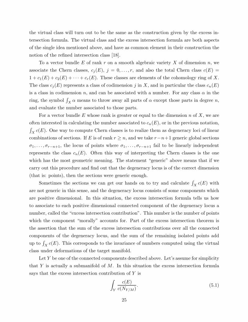
Let Y be one of the connected components described above. Let’s assume for simplicity

that Y is actually a submanifold of M . In this situation the excess intersection formula

says that the excess intersection contribution of Y is∫

Y

c(E)

c(NY/M). (5.1)

25

Here NY/M is the normal bundle of Y in M , and the expression after the integral sign

makes sense, since c(NY/M) is an element of a graded ring whose degree zero part is 1, and

so c(NY/M ) may be inverted in that ring.

5.1. Rational curves on the quintic threefold

As an example of an application of the excess intersection formula to explain the

significance of a calculation, let us review the count of the rational curves on a quintic

threefold as explained by Kontsevich [6] . Let Md = M00(d,P4) be the moduli space of

maps of genus zero curves of degree d to P4. Md is of dimension 5d+1. Let Ud be the vector

bundle on Md whose fiber at any stable map (C, f) is H0(C, f∗OP4(5)); this is a bundle of

rank 5d+ 1. The numbers Kd =∫

Mdc(Ud) have been computed by mirror symmetry, and

the first few are K1 = 2875, K2 = 4876875/8, and K3 = 8564575000/27. To try and find

a geometric interpretation of these numbers, we compute∫

Mdc(Ud) by finding a global

section of Ud and examining its degeneracy locus. Let F be a generic section of OP4(5)

on P4 which cuts out a smooth quintic threefold X . We pull F back to give us a global

section of Ud, which we call σd. The degeneracy locus of σd in Md consists of those maps

(C, f) with f(C) contained in this quintic threefold. This observation allows us to use the

Kd to compute the number of rational curves of degree d on the quintic threefold X .

In degree 1 the degeneracy locus consists of one point for every line mapping into X ,

and so we see that K1 = 2875 is the number of lines in a quintic threefold. In degree two,

the degeneracy locus of σ2 consists of an isolated point for every degree two rational curve

in X , and 2875 positive dimensional loci, each one consisting of maps which map two to

one onto a line in X . To calculate the actual number of degree two rational curves in

X , we compute the excess intersection contribution of each of these positive dimensional

components, and subtract from the previously computed total of 4876875/8. We now

compute this excess intersection contribution.

For each line l in X , let Yl be the submanifold of M2 parameterizing two to one covers

of l. The normal bundle of l in P4 is Nl/P4 = Ol(1)⊕Ol(1)⊕Ol(1). A calculation on the

tangent space of M2 shows that the normal bundle NYl/M2is (at a map (C, f)) equal to

H0(C, f∗Nl/P4).

Since the line l is sitting in the quintic threefold X , its normal bundle maps naturally

to the normal bundle of X in P4, with kernel the normal bundle of l in X . This gives us

an exact sequence:

26

0 −→ Ol(−1)⊕Ol(−1) −→ Nl/P4 −→ Ol(5) −→ 0.

Let V2 be the bundle on Yl whose fiber at a map (C, f) is H1(C, f∗Ol(−1)). The

above short exact sequence on l gives us the sequence

0 −→ NYl/M2−→ E2 −→ V2 ⊕ V2 −→ 0

of bundles on M2. The multiplicative properties of Chern classes in short exact sequences

shows us that the excess contribution of Yl is:∫

Yl

c(E2)

c(NYl/M2)

=

∫

Yl

c(V2)c(V2).

This last number is the Aspinwall-Morrison computation of 1/d3, or in this case,

1/8. This gives the number of actual degree two rational curves on a quintic threefold as

4876875/8− 2875/8 = 609250.

Under the assumption that each rational curve in X is isolated and smooth, then

similar computations give the famous formula [19]

Kd =∑

k|d

nd/kk3

, (5.2)

where nd is the number of rational curves in degree d. A caveat: It has been shown

that this assumption is false in at least one instance – in degree five, some of the rational

curves are plane curves with six nodes [20]. This doesn’t affect the computation until you

try to calculate multiple cover contributions from these curves. For example,6 in degree

ten we have double covers of these nodal curves. The moduli space of double covers of

a (once) nodal rational curve has two components: one being degree two maps to the

normalization of the nodal curve, which contributes 1/8 as for the smooth case; the other

being a single point representing two disconnected copies of the normalization mapping

down to the singular curve. If P,Q represent the points on the normalization which are

to be identified for the nodal curve, there is a uniqe map from a domain curve with two

components and one node, where the node is mapped to P on one copy and Q on the other

(these points are identified). This double cover does not factor through the normalization.

If we have n such curves, their double covers contribute n/8+n. The integers nd obtained

from the formula (5.2) need to be shifted to have the proper enumerative interpretation

(“experimentally,” this shift is integral, though this has not been proven [21] ).

6 We thank N. C. Leung for describing this example to us.

27

5.2. Calabi-Yau threefolds containing an algebraic surface

Let us consider the situation where we have a Calabi-Yau threefold, X, in a toric

variety, P, and a smooth algebraic surface, B, contained within X :

B ⊂ X ⊂ P. (5.3)

We assume as well that B is a Fano surface so that X may be deformed so that B shrinks

[22]. This is the scenario of interest to us in this paper. Now since there are holomorphic

maps of many degrees into B, which therefore all lie within X, we will have an enormous

degeneracy locus. If X is cut from some section s, then at degree β the whole space

M0,0(β;B) will be a zero set of the pull-back section s.7 Therefore, we will need to use

the excess intersection formula to calculate the contribution of the surface to the Gromov-

Witten invariants for X. From this, we will extract integers which account for the effective

number of curves due to B.

Mapping tangent vectors, we have from (5.3) the following exact sequence: 0 →

NB/X → NB/P → NX/P → 0. Note that NB/X = KB, by triviality of Λ3TX and the

exact sequence TB → TX → NB/X . Therefore, we have

0 −→ KB −→ NB/P −→ NX/P −→ 0.

Given (C, f) ∈ M0,0(β;B), we can pull back these bundles and form the long exact

sequence of cohomology:

0 −→ H0(C, f∗KB) −→ H0(C, f∗NB/P) −→ H0(C, f∗NX/P) −→

−→ H1(C, f∗KB) −→ H1(C, f∗NB/P) −→ ....(5.4)

Now H0(C, f∗KB) = 0 since B is Fano (its canonical bundle is negative), and

H1(C, f∗NB/P) = 0 when B is a complete intersection of (of nef divisors), which

we assume. As a result, (5.4) becomes a short exact sequence of the bundles over

M0,0(β;B) ⊂ M0,0(β;P) whose fibers are the corresponding cohomology groups. The

bundle (call it Uβ) with fiber H1(C, f∗KB) is the one we use to define the local invariants.

The bundle with fiber H0(C, f∗NB/P) is NM(B)/M(P) (abbreviating the notation a bit).

7 Actually, β labels a class in X which may be the image of a number of classes in B. In such a

case, our invariants are only sensitive to the image class, and represent a sum of invariants indexed

by classes in B.

28

That with fiber H0(C, f∗NX/P) is the one used to define the (global) Gromov-Witten

invariants for X – call it Eβ. Therefore, we have

0 −→ Uβ −→ NM(B)/M(P) −→ Eβ −→ 0.

Now using (5.1) with E = Eβ; M = M0,0(β;P); and Y = M0,0(β;B); the multi-

plicativity of the Chern class gives the contribution to the Gromov-Witten invariant of the

threefold X from a surface B ⊂ X is

Kβ =

∫

M0,0(β;B)

c(Uβ), (5.5)

which is what we have been computing.

Typically, the presence of a surface B ⊂ X may not be generic, so that X can

be deformed to a threefold X ′ not containing such a holomorphic surface. Let KXβ be

the Gromov-Witten invariant of X, and let KX′

β be the Gromow-Witten of X ′. These

are equal, as the Gromov-Witten invariant is an intersection independent of deformation:

KXβ = KX′

β . For X ′ we have an enumerative interpretation8 of KX′

β in terms of n′β, the

numbers of rational curves on X ′. Let nβ be the numbers of rational curves on X, and let

Kβ be the integral in (5.5). For simplicity, let us assume that dimH2(X′) = 1, so that

degree is labeled by an integer: β = d. Then combining the enumerative interpretation

with the interpretation of the excess intersection above, we find

KX′

d =∑

k|d

n′d/k/k

3 =∑

k|d

nd/k/k3 +Kd.

Subtracting, we find

Kd =∑

k|d

δnd/k/k3.

Here δn = n′−n represents the effective number of curves coming from B. In the text, we

typically write n for δn.

We therefore have an enumerative interpretation of the local invariants. After per-

forming the 1/d3 reduction we get an integer representing an effective number of curves

(modulo multiple covers of singular curves, which should shift these integers). We should

note that one might ask about rational curves in the Calabi-Yau manifold which intersect

our Fano surface. Such a situation would make for a more complicated degeneracy locus,

8 Singular rational curves notwithstanding.

29

but it turns out this situation does not arise. Indeed, if C′ ⊂ X is a holomorphic curve in

X meeting B transversely, then C′ ·B > 0 (strictly greater). However, for C ⊂ B, we have

C ·B =

∫

D

c1(NB/X) =

∫

D

c1(KB) < 0,

by the Fano condition. Therefore, C′ cannot lie in the image of H2(B) in H2(X) – the

only classes in which we are interested – and so our understanding of the numbers nd is

therefore complete.

5.3. Singular geometries

For physical applications, we will often want the surface B to be singular. For ex-

ample, in order to geometrically engineer SU(n + 1) supersymmetric gauge theories in

four dimensions, we consider the local geometry of an An singularity fibered over a P1.

In fact, we take a resolution along each An fiber, so that the exceptional divisor over a

point is a set of P1’s intersecting according to the Dynkin diagram of SU(n + 1). The

total geometry of these exceptional divisors forms a singular surface, which is a set of P1

bundles over P1 (Hirzebruch surfaces) intersecting along sections. In [3] it is shown how

the local invariants we calculate can be used to derive the instanton contributions to the

gauge couplings. Roughly speaking, the number of wrappings of the P1 base determines

the instanton number, while the growth with fiber degree of the number of curves with a

fixed wrapping along the base determines the corresponding invariant.

It is clearly of interest, then, to be able to handle singular geometries. Actually, we

will be able to do so without too much effort. Let us consider an illustrative example.

Define the singular surface B′ to be two P2’s intersecting in a P1. This can be thought of

as a singular quadric surface, since it can be represented as the zero locus of the reducible

degree two polynomial

XY = 0

in P3 with homogeneous coordinates [X, Y, Z].The generic smooth quadric is a surface B =

P1×P1. If we express B as a hypersurface in P3, we can define the local invariants (indexed

only by the generator of H2(P3)) of B as an intersection calculation in M0,0(d;P

3) as

follows. Define the bundle

E ≡ OP3(2)⊕OP3(−2).

Then let sE = (s, 0) be a global section of E, where s is a quadric and 0 is the only

global section of OP3(−2). Note that, by design, E restricted to the zero set of sE is

30

equal to KB . We now define a bundle over M0,0(d;P3) whose fibers over a point (C, f)

are H0(C, f∗OP3(2)) ⊕H1(C, f∗OP3(−2)). We then compute the top Chern class of the

bundle, which can be calculated as in the previous subsections in terms of the zero locus of

sE , which picks out maps into B ∼= P1×P1. The calculation gives the usual local invariant

for P1 ×P1, counting curves by their total degree d = d1 + d2, where di is the degree in

P1i , i = 1, 2. The reason is that O(2)|B = NB/P3 , so the contribution from this part to the

total Chern class cancels with the normal bundle to the map. (The local invariants are

listed in the first column of Table 7.)

Now note that this intersection calculation is independent of the section we use to

compute it. In fact, if we use a reducible quadric whose zero locus is B′, the calculation

will reduce to one on the singular spaceM0,0(d;B′). The excess intersection formula tells

us exactly which class to integrate over this (singular) space. In fact, integration over the

singular space is only defined via the virtual fundamental class – which is constructed to

yield the same answer. In degree one, this can all be checked explicitly in this example [23].

The upshot is that as our calculations are independent of deformations, we can deform

our singular geometries to do local calulations in a simpler setting. In fact, this makes

intuitive physical sense: the A-model should be independent of deformations.

Another phenomenon that we note in examples is that the calculation of the mirror

principle can be performed without reference to a specific bundle. In other words, the

toric data defining any non-compact Calabi-Yau threefold works as input data. As a

result, we can consider Calabi-Yau threefolds containing singular divisors and perform the

calculation. For the example of A2 fibered over a sphere, we get the numbers in Table

4. Though this technique has not yet been proven to work, it is tantalizing to guess that

the whole machinery makes sense for any non-compact threefold, with intersections taking

place in the Chow ring and with an appropriately defined prepotential.

In the next section, we will use the B-model to define differential equations whose

solutions determine the local contributions we have been discussing.

6. Local Mirror Symmetry: The B-Model

In this section we describe the mirror symmetry calculation of the Gromov-Witten

invariants for a (n − 1)-dimensional manifold B with c1(B) > 0. We first approach this

by using mirror symmetry for a compact, elliptically fibered Calabi-Yau n-fold9 X which

9 We will state formulas for n-folds, when possible.

31

contains B as a section, and taking then the volume of the fiber to infinity. If B is a Fano

manifold or comes from a (n− 1)-dimensional reflexive polyhedron a smooth Weierstrass

Calabi-Yau manifold X with B as a section exists. Moreover the geometry of X depends

only on B and therefore the limit can be described intrinsically from the geometry of B.

This is an intermediate step. Later, we will define the objects relevant for the B-model

calculation for B intrinsically, without referring to any embedding. Such an embedding,

in fact, is in general not possible.

6.1. Periods and differential equations for global mirror symmetry

We briefly review the global case in the framework of toric geometry, following the

ideas and notations of [24][25]. According to [24], a mirror pair (X, X) with the property

hp,q(X) = hn−p,q(X) can be represented as the zero locus of the Newton polynomials10

(P = 0, P = 0) associated to a dual pair of reflexive (n+1)-dimensional polyhedra (∆, ∆).

X is defined as hypersurface by the zero locus of

P =∑

ν(i)

ai

n+1∏

j=1

Xν(i)j

j (6.1)

in the toric ambient space PΣ(∆), constructed by the complete fan Σ(∆) associated to ∆.

The sum (6.1) runs over r “relevant” points ν(i) ∈ ∆, which do not lie on codimension

one faces and with ν(0) we denote the unique interior point in ∆. The ai parametrize the

complex structure deformations of X redundantly because of the induced (C∗)n+2 actions

on the ai, which compensate Xi → λiXi, P → λ0P, such that P = 0 is invariant. Invariant

complex structure coordinates are combinations

zi = (−1)l(j)0

r−1∏

j=0

al(i)j

j , (6.2)

where the l(j), j = 1, . . . , k = r − (n + 1) are an integral basis of linear relations among

the extended “relevant” points ν(i) = (1, ν(i)) with ν(i) ∈ rel(∆), i.e.

r−1∑

i=0

l(j)i ν(i) = ~0. (6.3)

10 The generalization to complete intersections in toric ambient spaces is worked out in [25][26].

32

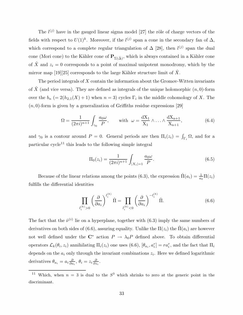
The l(j) have in the gauged linear sigma model [27] the role of charge vectors of the

fields with respect to U(1)k. Moreover, if the l(j) span a cone in the secondary fan of ∆,

which correspond to a complete regular triangulation of ∆ [28], then l(j) span the dual

cone (Mori cone) to the Kahler cone of PΣ(∆), which is always contained in a Kahler cone

of X and zi = 0 corresponds to a point of maximal unipotent monodromy, which by the

mirror map [19][25] corresponds to the large Kahler structure limit of X.

The period integrals ofX contain the information about the Gromov-Witten invariants

of X (and vice versa). They are defined as integrals of the unique holomorphic (n, 0)-form

over the bn (= 2(h2,1(X) + 1) when n = 3) cycles Γi in the middle cohomology of X . The

(n, 0)-form is given by a generalization of Griffiths residue expressions [29]

Ω =1

(2πi)n+1

∫

γ0

a0ω

P, with ω =

dX1

X1∧ . . . ∧

dXn+1

Xn+1, (6.4)

and γ0 is a contour around P = 0. General periods are then Πi(zi) =∫

ΓiΩ, and for a

particular cycle11 this leads to the following simple integral

Π0(zi) =1

(2πi)n+1

∫

|Xi|=1

a0ω

P. (6.5)

Because of the linear relations among the points (6.3), the expression Π(ai) = 1a0

Π(zi)

fulfills the differential identities

∏

l(k)i>0

(

∂

∂ai

)l(k)i

Π =∏

l(k)i<0

(

∂

∂ai

)−l(k)i

Π. (6.6)

The fact that the ν(i) lie on a hyperplane, together with (6.3) imply the same numbers of

derivatives on both sides of (6.6), assuring equality. Unlike the Π(zi) the Π(ai) are however

not well defined under the C∗ action P → λ0P defined above. To obtain differential

operators Lk(θi, zi) annihilating Πi(zi) one uses (6.6), [θai, ari ] = rari , and the fact that Πi

depends on the ai only through the invariant combinations zi. Here we defined logarithmic

derivatives θai= ai

∂∂ai

, θi = zi∂∂zi

.

11 Which, when n = 3 is dual to the S3 which shrinks to zero at the generic point in the

discriminant.

33

Example: X is the degree 18 hypersurface in P(1, 1, 1, 6, 9), with Euler number −540

and h1,1(X) = 2 and h2,1(X) = 272. The toric data are

a.) ∆ = conv[−6,−6, 1, 1], [−6, 12, 1, 1], [0, 0,−2, 1], [0, 0, 1,−1], [12,−6, 1, 1]

b.) rel(∆) = [0, 0, 0, 0]; [1, 0, 2, 3], [0, 1, 2, 3], [−1,−1, 2, 3], [0, 0, 2, 3], [0, 0,−1, 0], [0, 0, 0,−1]

c.) triang = [0, 1, 2, 4, 5], [0, 1, 3, 4, 5], [0, 1, 3, 4, 6], [0, 2, 3, 4, 5], [0, 1, 2, 4, 6], [0, 2, 3, 5, 6],

[0, 1, 2, 5, 6], [0, 1, 3, 5, 6], [0, 2, 3, 4, 6]

d.) SRI = x1 = x2 = x3 = 0, x4 = x5 = x6 = 0

e.) l(1) = (−6; 0, 0, 0, 1, 2, 3), l(2) = (0; 1, 1, 1,−3, 0, 0)

f.) J31 = 9 J2

1J2 = 3 J1J22 = 1, c2J1 = 102, c2J2 = 36.

(6.7)

Here triang is a regular star triangulation of ∆, where the 4d simplices are specified by

the indices of the points in rel(∆). SRI denotes the Stanley Reisner Ideal. JiJkJl and

c2Ji are the triple intersection numbers and the evaluation of the second chern class on

the forms Ji, i.e.∫

c2Ji. Then by (6.1) X is given by

P = a0 +X23X

34 (a1X1 + a2X2 +

a3

X1X2+ a4) +

a5

X3+a6

X4= a0 + Ξ

and the period (6.5) is easily integrated in the variables(6.2) z1 =a4a

25a

36

a60

, z2 = a1a2a3

a34

Π0 =1

(2πi)4

∫

1

1 + 1a0

Ξω =

[

∞∑

n=0

(

−Ξ

a0

)n]

term constant in Xi

=

[

∞∑

n=0

(−a0)−n

∑

ν1+...+ν6=n

(

n!

ν1! . . . ν6!

)

(a1X1X23X

34 )ν1 · · ·

(

a6

X4

)ν6]

term constant in Xi

=∞∑

r1=0,r2=0

Γ(6r1 + 1)

Γ(r2 + 1)3Γ(r1 − 3r2 + 1)Γ(3r1 + 1)Γ(2r1 + 1)zr11 z

r22 .

Likewise, it is easy to see that (6.6) leads to

L1 = θ1(θ1 − 3θ2)− 12(6θ1 − 5)(6θ1 − 1)z1

L2 = θ23 − (1 + θ1 − 3θ2)(2 + θ1 − 3θ2)(3 + θ1 − 3θ2)z2 ,

(6.8)

where we factored from the first operator a degree four differential operator. This is

equivalent to discarding four solutions which have incompatible behavior at the boundary

34

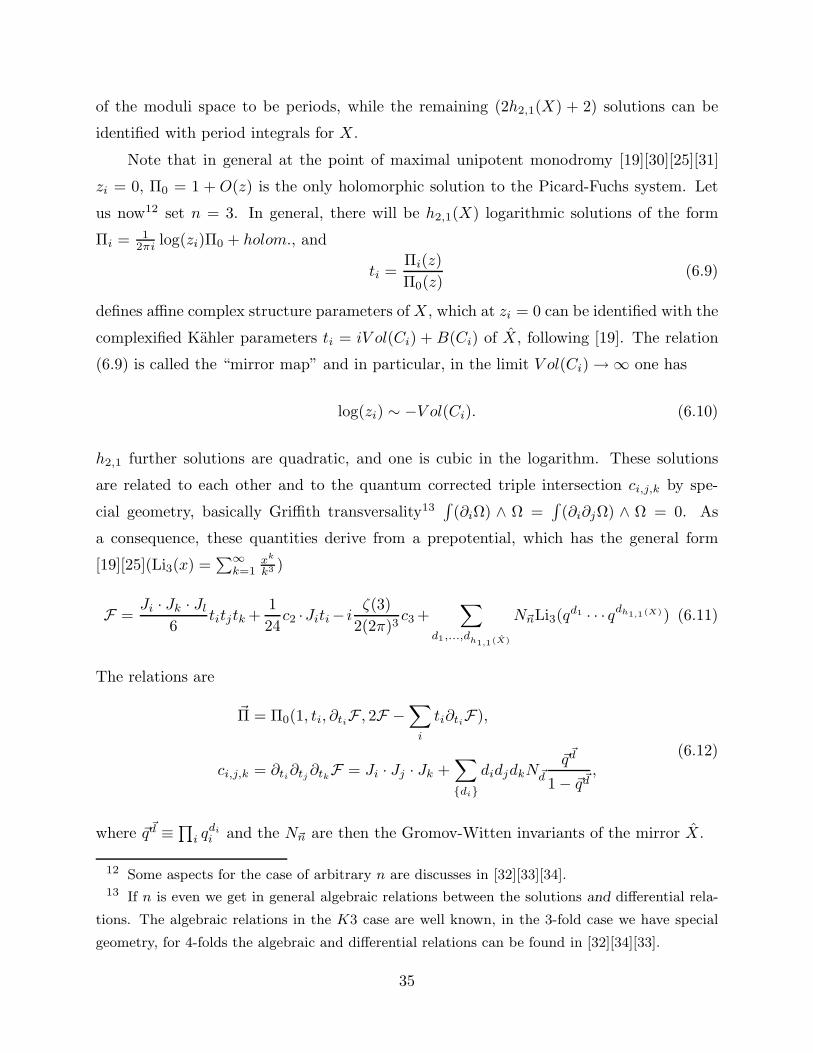
of the moduli space to be periods, while the remaining (2h2,1(X) + 2) solutions can be

identified with period integrals for X .

Note that in general at the point of maximal unipotent monodromy [19][30][25][31]

zi = 0, Π0 = 1 + O(z) is the only holomorphic solution to the Picard-Fuchs system. Let

us now12 set n = 3. In general, there will be h2,1(X) logarithmic solutions of the form

Πi = 12πi log(zi)Π0 + holom., and

ti =Πi(z)

Π0(z)(6.9)

defines affine complex structure parameters of X , which at zi = 0 can be identified with the

complexified Kahler parameters ti = iV ol(Ci) + B(Ci) of X, following [19]. The relation

(6.9) is called the “mirror map” and in particular, in the limit V ol(Ci)→∞ one has

log(zi) ∼ −V ol(Ci). (6.10)

h2,1 further solutions are quadratic, and one is cubic in the logarithm. These solutions

are related to each other and to the quantum corrected triple intersection ci,j,k by spe-

cial geometry, basically Griffith transversality13∫

(∂iΩ) ∧ Ω =∫

(∂i∂jΩ) ∧ Ω = 0. As

a consequence, these quantities derive from a prepotential, which has the general form

[19][25](Li3(x) =∑∞k=1

xk

k3 )

F =Ji · Jk · Jl

6titjtk+

1

24c2 ·Jiti− i

ζ(3)

2(2π)3c3 +

∑

d1,...,dh1,1(X)

N~nLi3(qd1 · · · qdh1,1(X)) (6.11)

The relations are

~Π = Π0(1, ti, ∂tiF , 2F −∑

i

ti∂tiF),

ci,j,k = ∂ti∂tj∂tkF = Ji · Jj · Jk +∑

di

didjdkN~d

~q~d

1− ~q~d,

(6.12)

where ~q~d ≡

∏

i qdi

i and the N~n are then the Gromov-Witten invariants of the mirror X.

12 Some aspects for the case of arbitrary n are discusses in [32][33][34].13 If n is even we get in general algebraic relations between the solutions and differential rela-

tions. The algebraic relations in the K3 case are well known, in the 3-fold case we have special

geometry, for 4-folds the algebraic and differential relations can be found in [32][34][33].

35

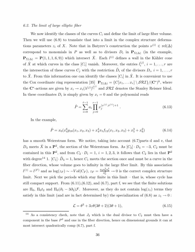
6.2. The limit of large elliptic fiber

We now identify the classes of the curves Ci and define the limit of large fiber volume.

Then we will use (6.9) to translate that into a limit in the complex structure deforma-

tions parameters zi of X . Note that in Batyrev’s construction the points ν(i) ∈ rel(∆)

correspond to monomials in P as well as to divisors Di in PΣ(∆) (in the example,

PΣ(∆) = P(1, 1, 1, 6, 9)) which intersect X. Each l(i) defines a wall in the Kahler cone

of X at which curves in the class [Ci] vanish. Moreover, the entries l(j)i , i = 1, . . . , r are

the intersection of these curves Cj with the restriction Di of the divisors Di, i = 1, . . . , r

to X. From this information one can identify the classes [Ci] in X . It is convenient to use

the Cox coordinate ring representation [35] PΣ(∆) = C[x1, . . . xr] \ SRI/(C∗)k, where

the C∗-actions are given by xi → xi(λ(j))l

(j)i and SRI denotes the Stanley Reisner Ideal.

In these coordinates Di is simply given by xi = 0 and the polynomial reads

P =r−1∑

i=0

ai

r−1∏

j=0

x〈ν(j),ν(i)〉+1j . (6.13)

In the example,

P = x0(x64g18(x1, x2, x3) + x4

4x5f12(x1, x2, x3) + x35 + x2

6) (6.14)

has a smooth Weierstrass form. We notice, taking into account (6.7)parts d and e, that

D4 meets X in a P2, the section of the Weierstrass form. As [C2] ·D4 = −3, C2 must be

contained in this P2, and from C2 ·Di = 1, i = 1, 2, 3, it follows that C2 lies in that P2

with degree14 1. [C1] · D4 = 1, hence C1 meets the section once and must be a curve in the

fiber direction, whose volume goes to infinity in the large fiber limit. By this association

l(1) = l(F ) and as log(zF ) ∼ −V ol(CF ), zF =a4a

26a

36

a60→ 0 is the correct complex structure

limit. Next we pick the periods which stay finite in this limit – that is, whose cycle has

still compact support. From (6.11),(6.12), and (6.7), part f, we see that the finite solutions

are Π0, Π0t2 and Π0(∂1 − 3∂2)F . Moreover, as they do not contain log(z1) terms they

satisfy in this limit (and are in fact determined by) the specialization of (6.8) as z1 → 0 :

L = θ3 + 3zθ(3θ + 2)(3θ + 1), (6.15)

14 As a consistency check, note that J2 which is the dual divisor to C2 must then have a

component in the base P 2 and one in the fiber direction, hence on dimensional grounds it can at

most intersect quadratically comp (6.7), part f.

36

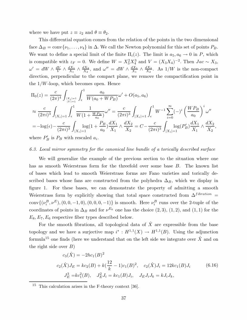
where we have put z ≡ z2 and θ ≡ θ2.

This differential equation comes from the relation of the points in the two dimensional

face ∆B = convν1, . . . , ν4 in ∆. We call the Newton polynomial for this set of points PB.

We want to define a special limit of the finite Πi(z). The limit is a5, a6 → 0 in P , which

is compatible with zF = 0. We define W = X23X

34 and V = (X3X4)

−2. Then Jac ∼ X3,

ω′ = dW ∧ dVV ∧

dX1

X1∧ dX2

X2, and ω′′ = dW ∧ dX1

X1∧ dX2

X2. As 1/W is the non-compact

direction, perpendicular to the compact plane, we remove the compactification point in

the 1/W -loop, which becomes open. Hence

Π0(z) =c

(2π)4

∫

|Xi|=1

|V |=1

∫ 1

ǫ

a0

W (a0 +WPB)ω′ +O(a5, a6)

≈c

(2πi)3

∫

|Xi|=1

∫ 1

ǫ

1

W (1 + WPB

a0)ω′′ =

c

(2πi)3

∫

|Xi|=1

∫ 1

ǫ

W−1∞∑

i=0

(−)i(

WPBa0

)i

ω′′

=−log(ǫ)−c

(2πi)3

∫

|Xi|=1

log(1 +PBa0

)dX1

X1∧dX2

X2= C−

c

(2πi)3

∫

|Xi|=1

log(P ′B)dX1

X1∧dX2

X2,

where P ′B is PB with rescaled ai.

6.3. Local mirror symmetry for the canonical line bundle of a torically described surface

We will generalize the example of the previous section to the situation where one

has as smooth Weierstrass form for the threefold over some base B. The known list

of bases which lead to smooth Weierstrass forms are Fano varieties and torically de-

scribed bases whose fans are constructed from the polyhedra ∆B , which we display in

figure 1. For these bases, we can demonstrate the property of admitting a smooth

Weierstrass form by explicitly showing that total space constructed from ∆fibration =

conv(νBi , νE), (0, 0,−1, 0), (0, 0, 0,−1) is smooth. Here νBi runs over the 2-tuple of the

coordinates of points in ∆B and for νEk one has the choice (2, 3), (1, 2), and (1, 1) for the

E8, E7, E6 respective fiber types described below.

For the smooth fibrations, all topological data of X are expressible from the base

topology and we have a surjective map i∗ : H1,1(X) → H1,1(B). Using the adjunction

formula15 one finds (here we understand that on the left side we integrate over X and on

the right side over B)

c3(X) = −2hc1(B)2

c2(X)JE = kc2(B) + k(12

k− 1)c1(B)2, c2(X)Ji = 12kc1(B)Ji

J3E =kc21(B), J2

EJi = kc1(B)Ji, JEJiJk = kJiJk,

(6.16)

15 This calculation arises in the F-theory context [36].

37

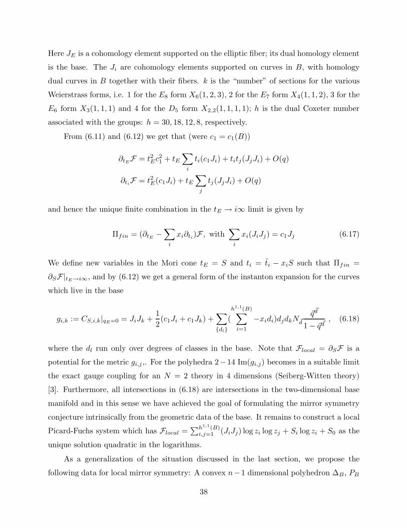
Here JE is a cohomology element supported on the elliptic fiber; its dual homology element

is the base. The Ji are cohomology elements supported on curves in B, with homology

dual curves in B together with their fibers. k is the “number” of sections for the various

Weierstrass forms, i.e. 1 for the E8 form X6(1, 2, 3), 2 for the E7 form X4(1, 1, 2), 3 for the

E6 form X3(1, 1, 1) and 4 for the D5 form X2,2(1, 1, 1, 1); h is the dual Coxeter number

associated with the groups: h = 30, 18, 12, 8, respectively.

From (6.11) and (6.12) we get that (were c1 = c1(B))

∂tEF = t2Ec21 + tE

∑

i

ti(c1Ji) + titj(JjJi) +O(q)

∂tiF = t2E(c1Ji) + tE∑

j

tj(JjJi) +O(q)

and hence the unique finite combination in the tE → i∞ limit is given by

Πfin = (∂tE −∑

i

xi∂ti)F , with∑

i

xi(JiJj) = c1Jj (6.17)

We define new variables in the Mori cone tE = S and ti = ti − xiS such that Πfin =

∂SF|tE→i∞, and by (6.12) we get a general form of the instanton expansion for the curves

which live in the base

gi,k := CS,i,k|qE=0 = JiJk +1

2(c1Ji + c1Jk) +

∑

dl

(

h1,1(B)∑

i=1

−xidi)djdkN~d

~q~d

1− ~q~d, (6.18)

where the dl run only over degrees of classes in the base. Note that Flocal = ∂SF is a

potential for the metric gi,j ,. For the polyhedra 2−14 Im(gi,j) becomes in a suitable limit

the exact gauge coupling for an N = 2 theory in 4 dimensions (Seiberg-Witten theory)

[3]. Furthermore, all intersections in (6.18) are intersections in the two-dimensional base

manifold and in this sense we have achieved the goal of formulating the mirror symmetry

conjecture intrinsically from the geometric data of the base. It remains to construct a local

Picard-Fuchs system which has Flocal =∑h1,1(B)i,j=1 (JiJj) log zi log zj + Si log zi + S0 as the

unique solution quadratic in the logarithms.

As a generalization of the situation discussed in the last section, we propose the

following data for local mirror symmetry: A convex n−1 dimensional polyhedron ∆B , PB

38

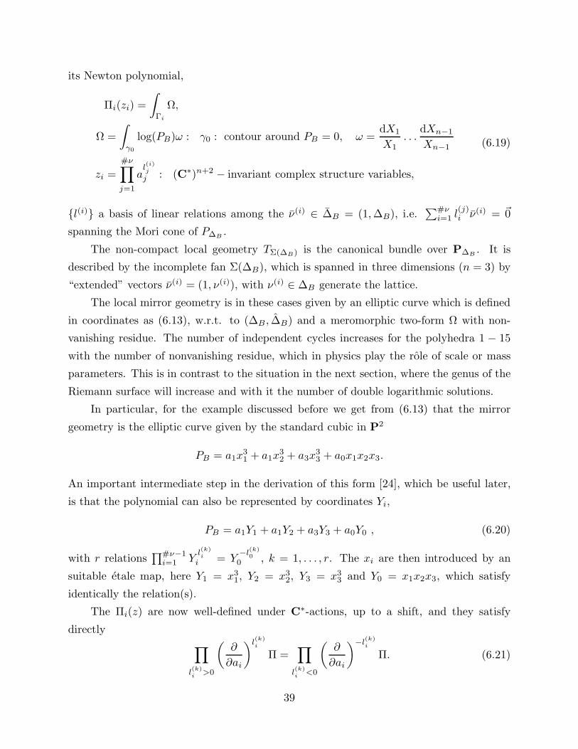
its Newton polynomial,

Πi(zi) =

∫

Γi

Ω,

Ω =

∫

γ0

log(PB)ω : γ0 : contour around PB = 0, ω =dX1

X1. . .

dXn−1

Xn−1

zi =

#ν∏

j=1

al(i)j

j : (C∗)n+2 − invariant complex structure variables,

(6.19)

l(i) a basis of linear relations among the ν(i) ∈ ∆B = (1,∆B), i.e.∑#νi=1 l

(j)i ν(i) = ~0

spanning the Mori cone of P∆B.

The non-compact local geometry TΣ(∆B) is the canonical bundle over P∆B. It is

described by the incomplete fan Σ(∆B), which is spanned in three dimensions (n = 3) by

“extended” vectors ν(i) = (1, ν(i)), with ν(i) ∈ ∆B generate the lattice.

The local mirror geometry is in these cases given by an elliptic curve which is defined

in coordinates as (6.13), w.r.t. to (∆B , ∆B) and a meromorphic two-form Ω with non-

vanishing residue. The number of independent cycles increases for the polyhedra 1 − 15

with the number of nonvanishing residue, which in physics play the role of scale or mass

parameters. This is in contrast to the situation in the next section, where the genus of the

Riemann surface will increase and with it the number of double logarithmic solutions.

In particular, for the example discussed before we get from (6.13) that the mirror

geometry is the elliptic curve given by the standard cubic in P2

PB = a1x31 + a1x

32 + a3x

33 + a0x1x2x3.

An important intermediate step in the derivation of this form [24], which be useful later,

is that the polynomial can also be represented by coordinates Yi,

PB = a1Y1 + a1Y2 + a3Y3 + a0Y0 , (6.20)

with r relations∏#ν−1i=1 Y

l(k)i

i = Y−l

(k)0

0 , k = 1, . . . , r. The xi are then introduced by an

suitable etale map, here Y1 = x31, Y2 = x3

2, Y3 = x33 and Y0 = x1x2x3, which satisfy

identically the relation(s).

The Πi(z) are now well-defined under C∗-actions, up to a shift, and they satisfy

directly

∏

l(k)i>0

(

∂

∂ai

)l(k)i

Π =∏

l(k)i<0

(

∂

∂ai

)−l(k)i

Π. (6.21)

39

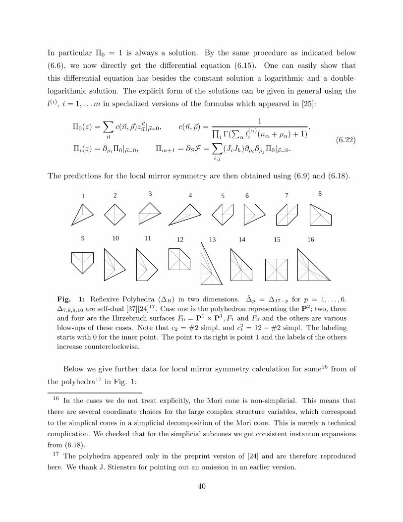
In particular Π0 = 1 is always a solution. By the same procedure as indicated below

(6.6), we now directly get the differential equation (6.15). One can easily show that

this differential equation has besides the constant solution a logarithmic and a double-

logarithmic solution. The explicit form of the solutions can be given in general using the

l(i), i = 1, . . .m in specialized versions of the formulas which appeared in [25]:

Π0(z) =∑

~n

c(~n, ~ρ)z~n~n |~ρ=0, c(~n, ~ρ) =1

∏

i Γ(∑

α l(α)i (nα + ρα) + 1)

,

Πi(z) = ∂ρiΠ0|~ρ=0, Πm+1 = ∂SF =

∑

i,j

(JiJk)∂ρi∂ρj

Π0|~ρ=0.(6.22)

The predictions for the local mirror symmetry are then obtained using (6.9) and (6.18).

1 2 4 5 6 7 83

9 10 11 15141312 16

Fig. 1: Reflexive Polyhedra (∆B) in two dimensions. ∆p = ∆17−p for p = 1, . . . , 6.

∆7,8,9,10 are self-dual [37][24]17. Case one is the polyhedron representing the P2; two, three

and four are the Hirzebruch surfaces F0 = P1 × P1, F1 and F2 and the others are various

blow-ups of these cases. Note that c2 = #2 simpl. and c21 = 12 − #2 simpl. The labeling

starts with 0 for the inner point. The point to its right is point 1 and the labels of the others

increase counterclockwise.

Below we give further data for local mirror symmetry calculation for some16 from of

the polyhedra17 in Fig. 1:

16 In the cases we do not treat explicitly, the Mori cone is non-simplicial. This means that

there are several coordinate choices for the large complex structure variables, which correspond

to the simplical cones in a simplicial decomposition of the Mori cone. This is merely a technical

complication. We checked that for the simplicial subcones we get consistent instanton expansions

from (6.18).17 The polyhedra appeared only in the preprint version of [24] and are therefore reproduced

here. We thank J. Stienstra for pointing out an omission in an earlier version.

40

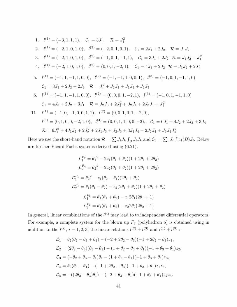
1. l(1) = (−3, 1, 1, 1), C1 = 3J1, R = J21

2. l(1) = (−2, 1, 0, 1, 0), l(2) = (−2, 0, 1, 0, 1), C1 = 2J1 + 2J2, R = J1J2

3. l(1) = (−2, 1, 0, 1, 0), l(2) = (−1, 0, 1,−1, 1), C1 = 3J1 + 2J2 R = J1J2 + J21

4. l(1) = (−2, 1, 0, 1, 0), l(2) = (0, 0, 1,−2, 1), C1 = 4J1 + 2J2 R = J1J2 + 2J21

5. l(1) = (−1, 1,−1, 1, 0, 0), l(2) = (−1,−1, 1, 0, 0, 1), l(3) = (−1, 0, 1,−1, 1, 0)

C1 = 3J1 + 2J2 + 2J3 R = J21 + J2J1 + J1J3 + J2J3

6. l(1) = (−1, 1,−1, 1, 0, 0), l(2) = (0, 0, 0, 1,−2, 1), l(3) = (−1, 0, 1,−1, 1, 0)

C1 = 4J3 + 2J2 + 3J1 R = J2J3 + 2J23 + J2J1 + 2J3J1 + J2

1

11. l(1) = (−1, 0,−1, 0, 0, 1, 1), l(2) = (0, 0, 1, 0, 1,−2, 0),

l(3) = (0, 1, 0, 0,−2, 1, 0), l(4) = (0, 0, 1, 1, 0, 0,−2), C1 = 6J1 + 4J2 + 2J3 + 3J4

R = 6J21 + 4J1J2 + 2J2

2 + 2J1J3 + J2J3 + 3J1J4 + 2J2J4 + J3J4J24

Here we use the short-hand notationR =∑

JiJk∫

BJiJk and C1 =

∑

i Ji∫

c1(B)Ji. Below

are further Picard-Fuchs systems derived using (6.21).

LF01 = θ1

2 − 2z1(θ1 + θ2)(1 + 2θ1 + 2θ2)

LF02 = θ2

2 − 2z2(θ1 + θ2)(1 + 2θ1 + 2θ2)

LF11 = θ2

2 − z1(θ2 − θ1)(2θ1 + θ2)

LF12 = θ1(θ1 − θ2)− z2(2θ1 + θ2)(1 + 2θ1 + θ2)

LF21 = θ1(θ1 + θ2)− z12θ1(2θ1 + 1)

LF22 = θ1(θ1 + θ2)− z22θ2(2θ2 + 1)

In general, linear combinations of the l(i) may lead to to independent differential operators.

For example, a complete system for the blown up F2 (polyhedron 6) is obtained using in

addition to the l(i), i = 1, 2, 3, the linear relations l(2) + l(3) and l(1) + l(3) :

L1 = θ2(θ2 − θ3 + θ1)− (−2 + 2θ2 − θ3)(−1 + 2θ2 − θ3)z1,

L2 = (2θ2 − θ3)(θ3 − θ1)− (1 + θ2 − θ3 + θ1)(−1 + θ3 + θ1)z2,

L3 = (−θ2 + θ3 − θ1)θ1 − (1 + θ3 − θ1)(−1 + θ3 + θ1)z3,

L4 = θ2(θ3 − θ1)− (−1 + 2θ2 − θ3)(−1 + θ3 + θ1)z1z2,

L5 = −((2θ2 − θ3)θ1)− (−2 + θ3 + θ1)(−1 + θ3 + θ1)z2z3.

41

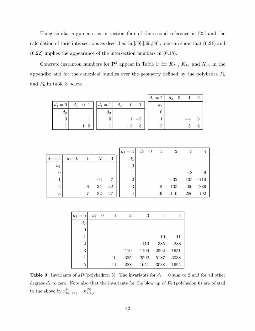
Using similar arguments as in section four of the second reference in [25] and the

calculation of toric intersections as described in [38],[39],[40], one can show that (6.21) and

(6.22) implies the appearance of the intersection numbers in (6.18).

Concrete instanton numbers for P2 appear in Table 1; for KF0, KF1

and KF2in the

appendix; and for the canonical bundles over the geometry defined by the polyhedra P5

and P6 in table 3 below.

d1 = 0 d3 0 1

d2

0 1

1 1 0

d1 = 1 d3 0 1

d2

0 1 −2

1 −2 3

d1 = 2 d3 0 1 2

d2

0

1 −4 5

2 5 −6

d1 = 3 d3 0 1 2 3

d2

0

1 −6 7

2 −6 35 −32

3 7 −32 27

d1 = 4 d3 0 1 2 3 4

d2

0

1 −8 9

2 −32 135 −110

3 −8 135 −400 286

4 9 −110 286 −192

d1 = 5 d3 0 1 2 3 4 5

d2

0

1 −10 11

2 −110 385 −288

3 −110 1100 −2592 1651

4 −10 385 −2592 5187 −3038

5 11 −288 1651 −3038 1695

Table 3: Invariants of dP2(polyhedron 5). The invariants for d1 = 0 sum to 2 and for all other

degrees d1 to zero. Note also that the invariants for the blow up of F2 (polyhedon 6) are related

to the above by n(6)k,i,i+j

= n(5)k,i,j

.

42

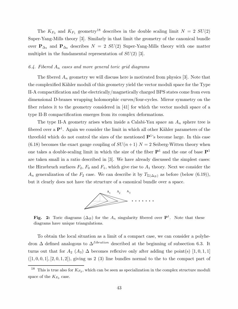
The KF0and KF1

geometry18 describes in the double scaling limit N = 2 SU(2)

Super-Yang-Mills theory [3]. Similarly in that limit the geometry of the canonical bundle

over P∆5and P∆6

describes N = 2 SU(2) Super-Yang-Mills theory with one matter

multiplet in the fundamental representation of SU(2) [3].

6.4. Fibered An cases and more general toric grid diagrams

The fibered An geometry we will discuss here is motivated from physics [3]. Note that

the complexified Kahler moduli of this geometry yield the vector moduli space for the Type

II-A compactification and the electrically/magnetically charged BPS states come from even

dimensional D-branes wrapping holomorphic curves/four-cycles. Mirror symmetry on the

fiber relates it to the geometry considered in [41] for which the vector moduli space of a

type II-B compactification emerges from its complex deformations.

The type II-A geometry arises when inside a Calabi-Yau space an An sphere tree is

fibered over a P1. Again we consider the limit in which all other Kahler parameters of the

threefold which do not control the sizes of the mentioned P1’s become large. In this case

(6.18) becomes the exact gauge coupling of SU(n+1) N = 2 Seiberg-Witten theory when

one takes a double-scaling limit in which the size of the fiber P1 and the one of base P1

are taken small in a ratio described in [3]. We have already discussed the simplest cases:

the Hirzebruch surfaces F2, F0 and F1, which give rise to A1 theory. Next we consider the

An generalization of the F2 case. We can describe it by TΣ(∆B) as before (below (6.19)),

but it clearly does not have the structure of a canonical bundle over a space.

AA

. . . . . . . A

1 2 3

Fig. 2: Toric diagrams (∆B) for the An singularity fibered over P1. Note that these

diagrams have unique triangulations.

To obtain the local situation as a limit of a compact case, we can consider a polyhe-

dron ∆ defined analogous to ∆fibration described at the beginning of subsection 6.3. It

turns out that for A2 (A3) ∆ becomes reflexive only after adding the point(s) [1, 0, 1, 1]

([1, 0, 0, 1], [2, 0, 1, 2]), giving us 2 (3) line bundles normal to the to the compact part of

18 This is true also for KF2 , which can be seen as specialization in the complex structure moduli

space of the KF0 case.

43

the local geometry. This is true more generally, i.e. one has n line bundles for An, but

for large n it is not possible to embed the An singularity in a compact Calabi-Yau space.

The n normal directions in the Kahler moduli space mean that the limit (6.17) leads to an

n-dimensional linear space of finite double-logarithmic solutions whose coefficients reflect

the directions in the normal Kahler moduli space in which the limit can be taken and for

combinatorial reasons their number corresponds to the number of ‘inner’ points in the toric

diagram. We denote a basis for these directions Si, i = 1, . . . , n. The n double-logarithmic

solutions come as we will see, given the meromorphic differential (6.19), from a genus n

Riemann surface for the local mirror. The Gromov-Witten invariants, on the other hand,

should not depend on the direction of the limit we take to obtain Πfin before matching

it to the N~d in (6.18). They therefore become rather non-trivial invariants of the differ-

ential system (6.21). In the following, we explicitly describe for all n the solutions of this

system corresponding to a preferred period basis, up to a choice of the double-logarithmic

solutions.

The generators of linear relations are

l(b) = (1, 1,−2, 0, 0, 0, 0, . . . , 0, 0, 0, 0),

l(1) = (0, 0, 1,−2, 1, 0, 0, . . . , 0, 0, 0, 0),

l(2) = (0, 0, 0, 1,−2, 1, 0, . . . , 0, 0, 0, 0),

......

l(n−1) = (0, 0, 0, 0, 0, 0, 0, . . . , 1,−2, 1, 0),

l(n) = (0, 0, 0, 0, 0, 0, 0, . . . , 0, 1,−2, 1).

(6.23)

Using the etale map Y0 = zs, Y1 = sz , Y2 = s and Yk = stk−2, k = 3, . . . , n + 3, solving

Y0Y1 = Y 22 , YiYi+2 = Y 2

i+1, i = 2, . . . , n+ 1 on the polynomial P =∑n+3

i=0 aiYi one gets [3]

P = sz +s

z+ an+1s+ anst+ . . .+ b0st

n+1 . (6.24)

This can be indentified, upon going to an affine patch s = 1 after trivial redefinitions and

the [3] limit, with the genus n SU(n+ 1) curves for N = 2 Super-Yang-Mills theory [42].

To obtain the complete solutions of the period system to the local mirror geometry

(6.24), we have to specify the classical intersection terms in the n double-logarithmic

solutions ∂SiF . Using (6.23),(6.21), the relation between the ideal of the principal part

of the differential operator at the maximal unipotent point zi = 0 and the logarithmic

44

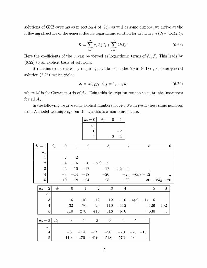
solutions of GKZ-systems as in section 4 of [25], as well as some algebra, we arrive at the

following structure of the general double-logarithmic solution for arbitrary n (Ji ∼ log(zi)):

R =n

∑

i=1

yiJi(Jb +i

∑

k=1

2kJk). (6.25)

Here the coefficients of the yi can be viewed as logarithmic terms of ∂SiF . This leads by

(6.22) to an explicit basis of solutions.

It remains to fix the xi by requiring invariance of the N~d in (6.18) given the general

solution (6.25), which yields

xi = Mi,jyj, i, j = 1, . . . , n , (6.26)

whereM is the Cartan matrix ofAn. Using this description, we can calculate the instantons

for all An.

In the following we give some explicit numbers for A2.We arrive at these same numbers

from A-model techniques, even though this is a non-bundle case.

db = 0 d2 0 1

d1

0 −2

1 −2 −2

db = 1 d2 0 1 2 3 4 5 6

d1

1 −2 −2

2 −4 −6 −6 −2d3 − 2 ..

3 −6 −10 −12 −12 −4d3 − 6 ..

4 −8 −14 −18 −20 −20 −6d3 − 12 ..

5 −10 −18 −24 −28 −30 −30 −8d3 − 20

db = 2 d2 0 1 2 3 4 5 6

d1

3 −6 −10 −12 −12 −10 −4(d3 − 1)− 6 ..

4 −32 −70 −96 −110 −112 −126 −192

5 −110 −270 −416 −518 −576 −630 ..

db = 3 d2 0 1 2 3 4 5 6

d1

4 −8 −14 −18 −20 −20 −20 −18

5 −110 −270 −416 −518 −576 −630 ..

45

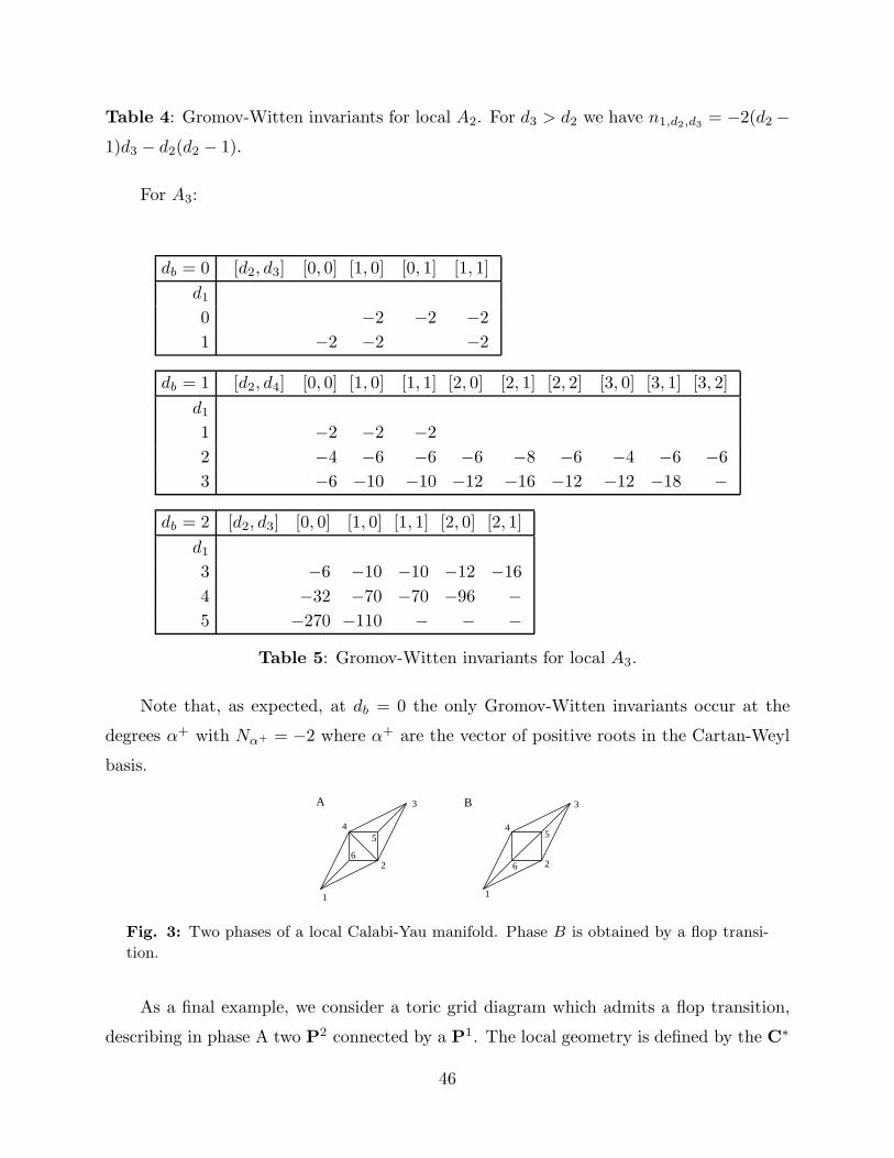
Table 4: Gromov-Witten invariants for local A2. For d3 > d2 we have n1,d2,d3 = −2(d2 −

1)d3 − d2(d2 − 1).

For A3:

db = 0 [d2, d3] [0, 0] [1, 0] [0, 1] [1, 1]

d1

0 −2 −2 −2

1 −2 −2 −2

db = 1 [d2, d4] [0, 0] [1, 0] [1, 1] [2, 0] [2, 1] [2, 2] [3, 0] [3, 1] [3, 2]

d1

1 −2 −2 −2

2 −4 −6 −6 −6 −8 −6 −4 −6 −6

3 −6 −10 −10 −12 −16 −12 −12 −18 −

db = 2 [d2, d3] [0, 0] [1, 0] [1, 1] [2, 0] [2, 1]

d1

3 −6 −10 −10 −12 −16

4 −32 −70 −70 −96 −

5 −270 −110 − − −

Table 5: Gromov-Witten invariants for local A3.

Note that, as expected, at db = 0 the only Gromov-Witten invariants occur at the

degrees α+ with Nα+ = −2 where α+ are the vector of positive roots in the Cartan-Weyl

basis.

1

4

3

2

1

2

3

45

6

5

6

A B

Fig. 3: Two phases of a local Calabi-Yau manifold. Phase B is obtained by a flop transi-

tion.

As a final example, we consider a toric grid diagram which admits a flop transition,

describing in phase A two P2 connected by a P1. The local geometry is defined by the C∗

46

operations generated by

l(1)A =( 0,−1, 0,−1, 1, 1), l

(1)B = ( 0, 1, 0, 1,−1,−1)

l(2)A =( 1, 1, 0, 1, 0,−3), l

(2)B = ( 1, 0, 0, 0, 1,−2)

l(3)A =( 0, 1, 1, 1,−3, 0), l

(3)B = ( 0, 0, 1, 0,−2, 1)

SRIA =x1 = x2 = x4 = 0, x5 = x6 = 0, SRIB = x2 = x4 = 0, x1 = x3 = 0,

x2 = x3 = x4 = 0, x1 = x3 = 0, x1 = x5 = 0, x3 = x6 = 0

x1 = x5 = 0, x3 = x6 = 0

and the indicated Stanley-Reisner ideal. As in the A2 case the mirror geometry is given by

a genus two Riemann surface. The space of double-logarithmic solutions is two dimensional

and can be determined from (6.21). Local invariants follow then for the A and B phase

via (6.18) from the following data

RA = y1J22 + y2(J

23 − J

22 ), xA1 = y1, xA2 = −3(y1 − y2), xA3 = −3y2

RB = y1(2J1J2 + J1J3 + 2J22 + J2

3 ) + y2(J22 + J1J2)

xB1 = y2, xB2 = −3y1 − 2y2, xB3 = −3y1 − y2 .

Below we list the Gromov-Witten invariants for the B phase of the (P2,P2) diagram

Fig. 3. The instantons of the A phase are related to the one in the B phase by nAk,j,i =

nBi+j−k,i,j . The only degree for which this formula does not apply is nA1,0,0 = 1, which

counts just the flopped P1.

db = 0 d2 0 1

d1

0 −2

1 −2 −2

db = 1 d2 0 1 2 3 4 5 6

d1

0 1 3 5 7 9 11 13

1 3 4 8 13 16 20 24

2 5 8 9 15 21 27 33

3 7 12 15 16 24 32 40

4 9 16 21 24 25 35 45

5 11 20 27 32 35 36 48

47

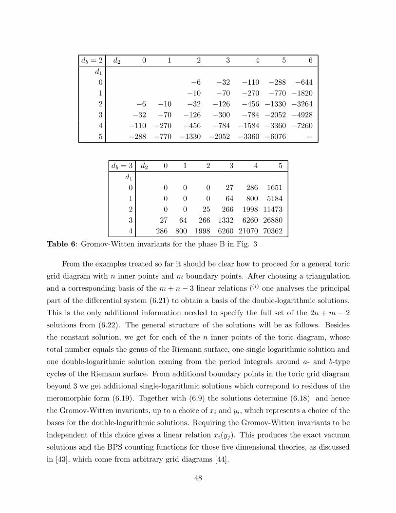
db = 2 d2 0 1 2 3 4 5 6

d1

0 −6 −32 −110 −288 −644

1 −10 −70 −270 −770 −1820

2 −6 −10 −32 −126 −456 −1330 −3264

3 −32 −70 −126 −300 −784 −2052 −4928

4 −110 −270 −456 −784 −1584 −3360 −7260

5 −288 −770 −1330 −2052 −3360 −6076 −

db = 3 d2 0 1 2 3 4 5

d1

0 0 0 0 27 286 1651

1 0 0 0 64 800 5184

2 0 0 25 266 1998 11473

3 27 64 266 1332 6260 26880

4 286 800 1998 6260 21070 70362

Table 6: Gromov-Witten invariants for the phase B in Fig. 3

From the examples treated so far it should be clear how to proceed for a general toric

grid diagram with n inner points and m boundary points. After choosing a triangulation

and a corresponding basis of the m+ n− 3 linear relations l(i) one analyses the principal

part of the differential system (6.21) to obtain a basis of the double-logarithmic solutions.

This is the only additional information needed to specify the full set of the 2n + m − 2

solutions from (6.22). The general structure of the solutions will be as follows. Besides

the constant solution, we get for each of the n inner points of the toric diagram, whose

total number equals the genus of the Riemann surface, one-single logarithmic solution and

one double-logarithmic solution coming from the period integrals around a- and b-type

cycles of the Riemann surface. From additional boundary points in the toric grid diagram

beyond 3 we get additional single-logarithmic solutions which correpond to residues of the

meromorphic form (6.19). Together with (6.9) the solutions determine (6.18) and hence

the Gromov-Witten invariants, up to a choice of xi and yi, which represents a choice of the

bases for the double-logarithmic solutions. Requiring the Gromov-Witten invariants to be

independent of this choice gives a linear relation xi(yj). This produces the exact vacuum

solutions and the BPS counting functions for those five dimensional theories, as discussed

in [43], which come from arbitrary grid diagrams [44].

48

6.5. Cases with constraints

The del Pezzo surfaces Bn can be constructed by blowing P2 up n times, 0 ≤ n ≤ 8, in

addition to P1×P1. As is well known, the case n = 6 can be represented as a cubic in P3

denoted byX3(1, 1, 1, 1), and n = 7, 8 are representable as degree four and six hypersurfaces

in weighted projective spaces: X4(1, 1, 1, 2) and X6(1, 1, 2, 3), respectively. The n = 5 case

can be represented as the degree (2,2) complete intersection in P4 X2,2(1, 1, 1, 1, 1). In

addition, the quadric in P3, X2(1, 1, 1, 1) is another representation of P1 × P1. In the

representation given for the non-local Calabi-Yau geometry as the canonical bundle over

this del Pezzo surfaces below, the map i∗ : H1,1(X) → H1,1(B) is not onto, as in the

previous cases. As a consequence the Gromow-Witten invariants are a sum over curves

with degree di in classes in H1,1(B) up to degree d =∑

i di. These cases have been

considered before [2][45][46][5].

As all the weights in these representations are co-prime, the Kahler class associated

to the hyperplane class of the ambient space is the only one which restricts to the surface

(no exceptional divisors from the ambient space). We can recast the Chern classes of the

surface and the of the canonical bundle over it in terms of this class J . This can be stated

more generally for smooth complete intersections by the definition of the following formal

weight or charge vectors l(k) = (d1(k), . . . , dr(k)|w1(k), . . . , ws(k)), where di(k) are the degree

of the i’th polynomial, i = 1, . . . , p, in the variables of the k’th weighted projective space,

k = 1, . . . , s. In terms of these we can express the total Chern class, by the adjunction

formula, to obtain the following formal expansion

c =

∏sk=1

∏r(k)

i=1(1 + wi,(k)J(k))∏pi=1(1 +

∑sk=1 di,(k)J(k))

∏pi=1

∑sk=1 dj,(k)J

(k)

∏sk=1

∏r(k)

i=1 wi,(k). (6.27)

Integrals over the top class for the non-compact case are formally defined by multiplying

with the volume form of the normal bundle V =∏tk=1

∏rj=1 dj,(k)J

(k) and picking the

coefficient of∏tk=1 J

(s(k)−1). Similarly wedge products of c2 with J and triple intersections

are obtained.19 We start by summarizing the weight or charge vectors for the non-compact

19 There are minor disagreements with the classical integrals equation (4.18) in [45] as well as

with the normalization of the instanton numbers for the case referred to as “conifold” in [45].

These data should all follow from (6.27).

49

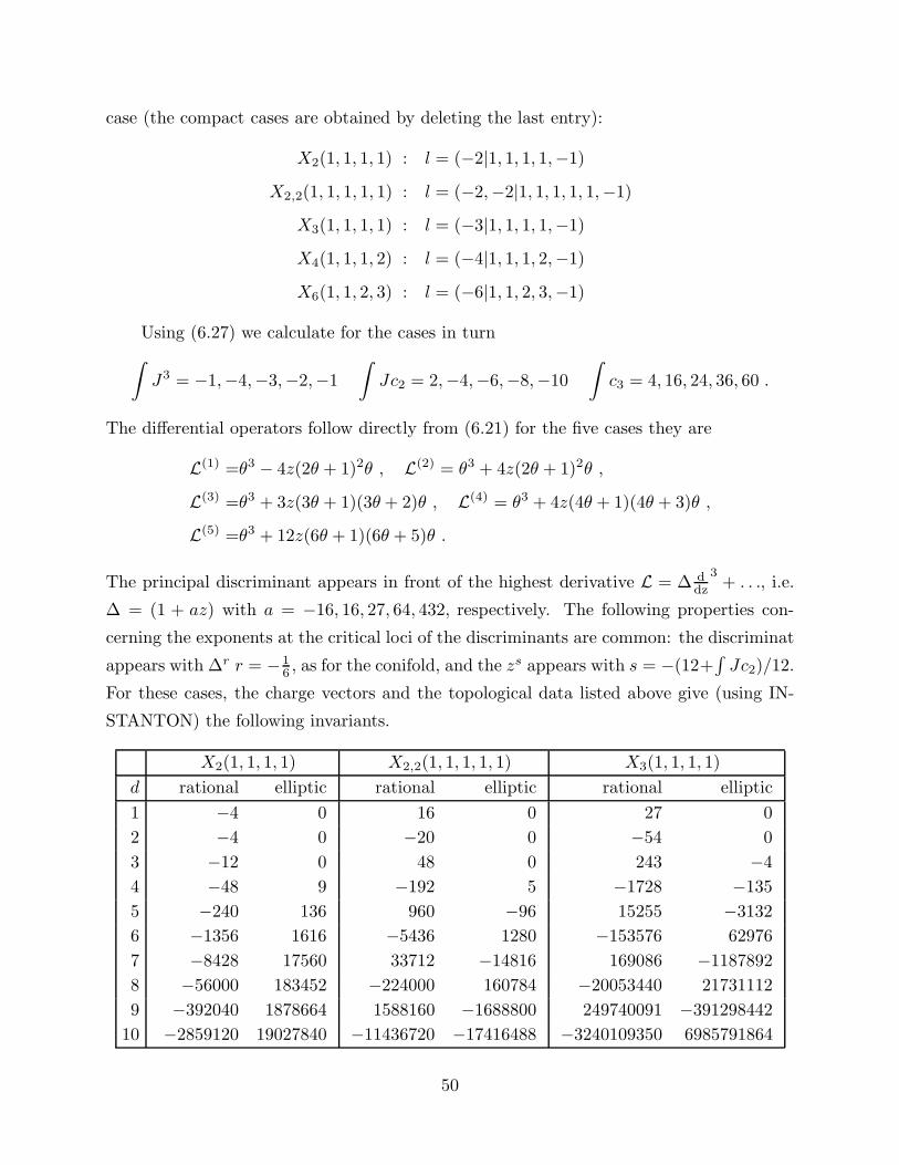
case (the compact cases are obtained by deleting the last entry):

X2(1, 1, 1, 1) : l = (−2|1, 1, 1, 1,−1)

X2,2(1, 1, 1, 1, 1) : l = (−2,−2|1, 1, 1, 1, 1,−1)

X3(1, 1, 1, 1) : l = (−3|1, 1, 1, 1,−1)

X4(1, 1, 1, 2) : l = (−4|1, 1, 1, 2,−1)

X6(1, 1, 2, 3) : l = (−6|1, 1, 2, 3,−1)

Using (6.27) we calculate for the cases in turn

∫

J3 = −1,−4,−3,−2,−1

∫

Jc2 = 2,−4,−6,−8,−10

∫

c3 = 4, 16, 24, 36, 60 .

The differential operators follow directly from (6.21) for the five cases they are

L(1) =θ3 − 4z(2θ + 1)2θ , L(2) = θ3 + 4z(2θ + 1)2θ ,

L(3) =θ3 + 3z(3θ + 1)(3θ + 2)θ , L(4) = θ3 + 4z(4θ + 1)(4θ + 3)θ ,

L(5) =θ3 + 12z(6θ + 1)(6θ + 5)θ .

The principal discriminant appears in front of the highest derivative L = ∆ ddz

3+ . . ., i.e.

∆ = (1 + az) with a = −16, 16, 27, 64, 432, respectively. The following properties con-

cerning the exponents at the critical loci of the discriminants are common: the discriminat

appears with ∆r r = −16 , as for the conifold, and the zs appears with s = −(12+

∫

Jc2)/12.

For these cases, the charge vectors and the topological data listed above give (using IN-

STANTON) the following invariants.

X2(1, 1, 1, 1) X2,2(1, 1, 1, 1, 1) X3(1, 1, 1, 1)

d rational elliptic rational elliptic rational elliptic

1 −4 0 16 0 27 0

2 −4 0 −20 0 −54 0

3 −12 0 48 0 243 −4

4 −48 9 −192 5 −1728 −135

5 −240 136 960 −96 15255 −3132

6 −1356 1616 −5436 1280 −153576 62976

7 −8428 17560 33712 −14816 169086 −1187892

8 −56000 183452 −224000 160784 −20053440 21731112

9 −392040 1878664 1588160 −1688800 249740091 −391298442

10 −2859120 19027840 −11436720 −17416488 −3240109350 6985791864

50

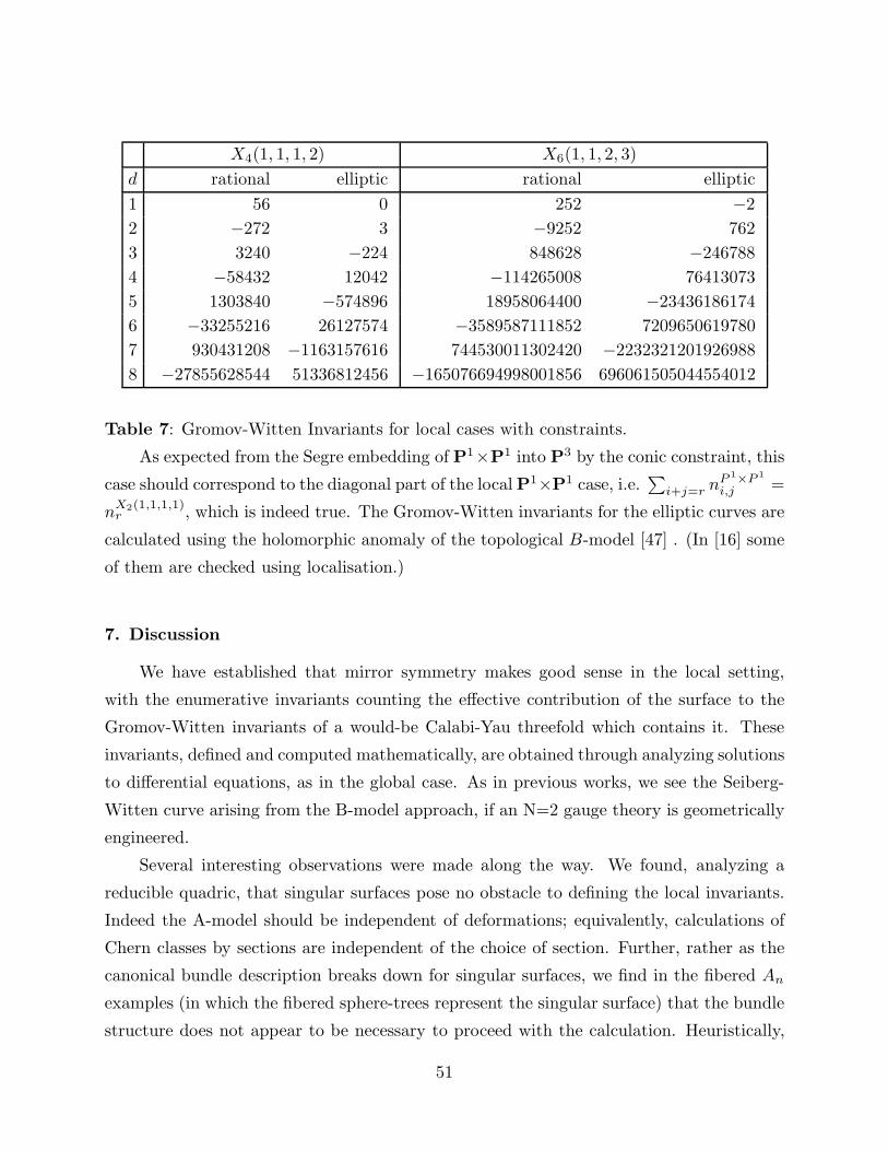
X4(1, 1, 1, 2) X6(1, 1, 2, 3)

d rational elliptic rational elliptic

1 56 0 252 −2

2 −272 3 −9252 762

3 3240 −224 848628 −246788

4 −58432 12042 −114265008 76413073

5 1303840 −574896 18958064400 −23436186174

6 −33255216 26127574 −3589587111852 7209650619780

7 930431208 −1163157616 744530011302420 −2232321201926988

8 −27855628544 51336812456 −165076694998001856 696061505044554012

Table 7: Gromov-Witten Invariants for local cases with constraints.

As expected from the Segre embedding of P1×P1 into P3 by the conic constraint, this

case should correspond to the diagonal part of the local P1×P1 case, i.e.∑

i+j=r nP 1×P 1

i,j =

nX2(1,1,1,1)r , which is indeed true. The Gromov-Witten invariants for the elliptic curves are

calculated using the holomorphic anomaly of the topological B-model [47] . (In [16] some

of them are checked using localisation.)

7. Discussion

We have established that mirror symmetry makes good sense in the local setting,

with the enumerative invariants counting the effective contribution of the surface to the

Gromov-Witten invariants of a would-be Calabi-Yau threefold which contains it. These

invariants, defined and computed mathematically, are obtained through analyzing solutions

to differential equations, as in the global case. As in previous works, we see the Seiberg-

Witten curve arising from the B-model approach, if an N=2 gauge theory is geometrically

engineered.

Several interesting observations were made along the way. We found, analyzing a

reducible quadric, that singular surfaces pose no obstacle to defining the local invariants.

Indeed the A-model should be independent of deformations; equivalently, calculations of

Chern classes by sections are independent of the choice of section. Further, rather as the

canonical bundle description breaks down for singular surfaces, we find in the fibered An

examples (in which the fibered sphere-trees represent the singular surface) that the bundle

structure does not appear to be necessary to proceed with the calculation. Heuristically,

51

one can model not just the moduli space of maps as a projective variety, but in fact the

whole vector bundle Ud. With intersections in the Chow ring and integration well-defined

by virtue of a Thom class, the procedure seems to yield the correct results. This technique

needs to be developed and made rigorous, but the numbers still agree with the B-model

results in Table 4-5.

The recent work of Vafa and Gopakumar [17] introduces a new interpretation of these

numbers and their analogues at higher genus. In particular, those authors count the

contributions of BPS states (D-branes) in a fixed homology class (but not fixed genus)

to the full string partition function, which is a sum over topological partition functions

at all genera. Their calculations tell us how to organize the partition functions in order

to extract integers, which represent BPS states corresponding to cohomology classes on

the full moduli space of BPS states20 and transforming under a certain SU(2) action in a

particular way. In genus zero, the contribution is equivalent to the Euler characteristic. At

degree three in P2, for example, a smooth degree three polynomial is an elliptic curve, and

the D-brane moduli space includes the choice of a U(1) bundle over the curve, equivalently

a point on the curve (if it is smooth). The choice of curves with points is shown in [17] to

be a P8 bundle over P2, a space with Euler characteristic 27 (which is indeed n3 for P2).

The singular curves, however, should be accompanied by their compactified Jacobians as

in [48], but these can in general no longer be equated with the curves themselves. Further,

the compactified Jacobians of reducible curves (e.g., the cubic XY Z = 0 in P2) are

particularly troublesome. Perhaps the non-compact direction in KP2 leads to a resolution

of these difficulties. It would be very interesting to mesh the Gromov-Witten and D-brane

explanations of these local invariants.

Having extended traditional mirror symmetry to the non-compact case, one naturally

asks whether other viewpoints of mirror symmetry make sense in the non-compact setting.

Is there any kind of special-Lagrangian fibration? It is likely that, if so, the fibers would

be decompactified tori, e.g. S1 × S1 × R. 21 This would be an interesting venue to the

conjectures of [50]. In particular, once the Kahler-Einstein metric of the surface is known,

Calabi [51] has given a method to find a Ricci-flat metric on the total space of the canonical

bundle. In [50] it is argued that not only should the total D-brane moduli space of the

special-Lagrangian torus be the mirror manifold, but also that the metric of the mirror

20 This is the standard reduction to a supersymmetric sigma model on a moduli space.21 Recently, [49] has found such a fibration for canonical bundles of projective spaces.

52

should be computable by an instanton expansion involving holomorphic discs bounding

the torus. The local setting of a degenerate fiber, such as has been studied and given an

explicit metric in [52], may prove an illustrative starting point (though several of us have

been unable to crack this example).

What about the categorical mirror symmetry conjecture of Kontsevich? Unfortu-

nately, few explicit descriptions are known of the derived categories of coherent sheaves

over non-compact spaces (or any spaces, for that matter). In two dimensions, however, the

recent work of [53] gives a description of the derived category over resolutions of A-D-E sin-

gularities in two dimensions. The fibered versions of these spaces are just what we consider

in this paper. It would be extremely interesting to calculate Fukaya’s category in these

examples, especially as we currently have a real dearth testing grounds for Kontsevich’s

ideas.

We feel that the local setting may be the best place for gleaning what’s really at work

in mirror symmetry and tying together our still fragmented understanding of this subject.

Acknowledgements

We are indebted to B. Lian, for explaining extensions of the mirror principle, and for

helping us at various stages of this project; and to M. Roth, for explaining many algebro-

geometric constructions and for his involvement at the early stages of our work. We thank

them, as well as T. Graber, R. Pandharipande, and C. Vafa for many helpful discussions.

The work of T.-M. Chiang and S.-T. Yau is supported in part by the NSF grant DMS-

9709694; that of A. Klemm in part by a DFG Heisenberg fellowship and NSF Math/Phys

DMS-9627351 and that of E. Zaslow in part by DE-F602-88ER-25065.

8. Appendix: Examples (A-Model)

8.1. O(4)→ P3

This case is very similar, only we note that the rank of Ud is 4d+1 and the dimension

of moduli space is 4d. Thus we must take the Chern class c4d integrated over the moduli

space. Taking the next-to-top Chern class has the following interpretation. Instead of just

counting the zeros of a section, s0, we take two sections s0 and s1 and look at the zeros of

s0 ∧ s1, i.e. we look for points where the two sections are not linearly independent. The

number of such points also has the following interpretation. Look at the P1 linear system

generated by s0 and s1. If s0 ∧ s1 has a zero at a point (C, f) in moduli space, then some

53

section as0+bs1 vanishes identically on f(C), i.e. f(C) maps to the zero locus of as0+bs1.

Therefore, the interpretation of the next-to-top Chern class is as the number of rational

curves in any member of the linear system generated by two linearly independent sections.

Of course, in this problem, we must account for multiple covers as above. After doing

so, the numbers nd which we get are as follows:

d nd

1 320

2 5016

3 144192

4 5489992

5 247634752

6 12472771416

7 678995926336

8 39156591980232

9 2360737982593344

10 147445147672907352

Table 8: Gromov-Witten invariants for a K3 surface inside a Calabi-Yau threefold.

Practically speaking, sections are simply quartic polynomials, and the zero loci are

quartic K3 surfaces. Therefore, we are counting the number of rational curves in a pencil

of quartic K3 surfaces. We may wish to compare our results with a Calabi-Yau manifold

admitting a K3 fibration. Of course, the number of curves will depend on the nature of the

fibration. Our count pertains to a trivial total family, i.e. the zero locus of a polynomial of

bi-degree (1, 4) in P1 ×P3. The degree 8 hypersurface Calabi-Yau manifold in P2,2,2,1,1 is

a pencil of quartic surfaces fibered over P1 in a different way, though the counting differs

only by a factor of two. Specifically, if we look at the Gromov-Witten invariants in the

homology class of d times the fiber (for this example h11 = 2, one class coming from the P1

base, one from the projective class of the K3 fiber), we get twice the numbers computed

above.

8.2. O(3)→ P2

In this example, the rank of Ud is now 3d+1 which is two greater than the dimension

of M00(d,P2), so we must take c(top−2)(Ud). The interpretation is similar to the case of

O(4)→ P3. We count the number of rational curves in a two-dimensional family of cubic

curves generated by three linearly independent sections of O(3) (cubics).

54

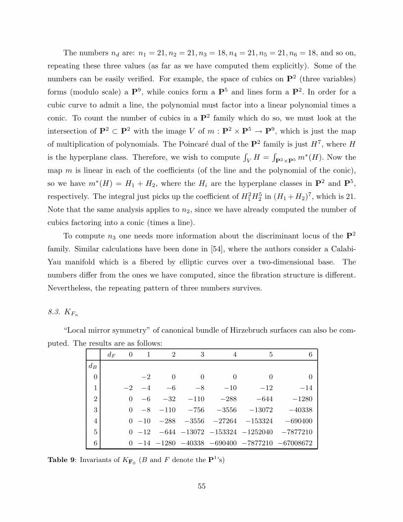
The numbers nd are: n1 = 21, n2 = 21, n3 = 18, n4 = 21, n5 = 21, n6 = 18, and so on,

repeating these three values (as far as we have computed them explicitly). Some of the

numbers can be easily verified. For example, the space of cubics on P2 (three variables)

forms (modulo scale) a P9, while conics form a P5 and lines form a P2. In order for a

cubic curve to admit a line, the polynomial must factor into a linear polynomial times a

conic. To count the number of cubics in a P2 family which do so, we must look at the

intersection of P2 ⊂ P2 with the image V of m : P2 × P5 → P9, which is just the map

of multiplication of polynomials. The Poincare dual of the P2 family is just H7, where H

is the hyperplane class. Therefore, we wish to compute∫

VH =

∫

P2×P5 m∗(H). Now the

map m is linear in each of the coefficients (of the line and the polynomial of the conic),

so we have m∗(H) = H1 + H2, where the Hi are the hyperplane classes in P2 and P5,

respectively. The integral just picks up the coefficient of H21H

52 in (H1 +H2)

7, which is 21.

Note that the same analysis applies to n2, since we have already computed the number of

cubics factoring into a conic (times a line).

To compute n3 one needs more information about the discriminant locus of the P2

family. Similar calculations have been done in [54], where the authors consider a Calabi-

Yau manifold which is a fibered by elliptic curves over a two-dimensional base. The

numbers differ from the ones we have computed, since the fibration structure is different.

Nevertheless, the repeating pattern of three numbers survives.

8.3. KFn

“Local mirror symmetry” of canonical bundle of Hirzebruch surfaces can also be com-

puted. The results are as follows:

dF 0 1 2 3 4 5 6

dB

0 −2 0 0 0 0 0

1 −2 −4 −6 −8 −10 −12 −14

2 0 −6 −32 −110 −288 −644 −1280

3 0 −8 −110 −756 −3556 −13072 −40338

4 0 −10 −288 −3556 −27264 −153324 −690400

5 0 −12 −644 −13072 −153324 −1252040 −7877210

6 0 −14 −1280 −40338 −690400 −7877210 −67008672

Table 9: Invariants of KF0(B and F denote the P1’s)

55

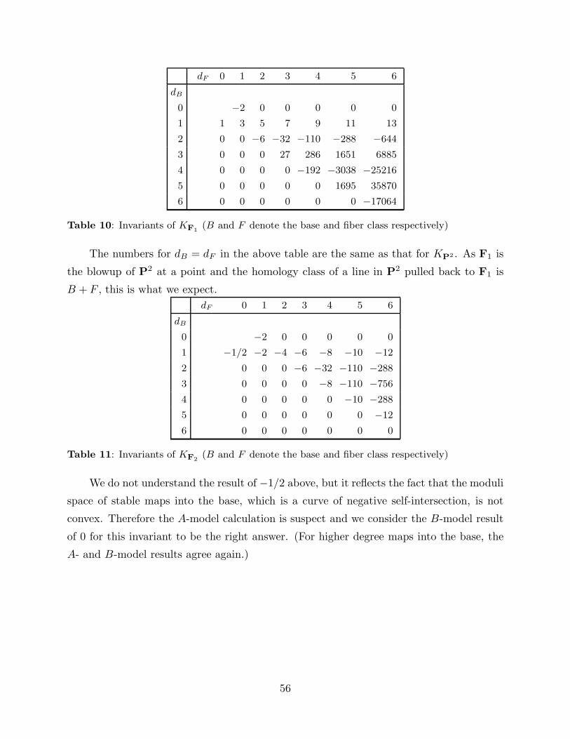
dF 0 1 2 3 4 5 6

dB

0 −2 0 0 0 0 0

1 1 3 5 7 9 11 13

2 0 0 −6 −32 −110 −288 −644

3 0 0 0 27 286 1651 6885

4 0 0 0 0 −192 −3038 −25216

5 0 0 0 0 0 1695 35870

6 0 0 0 0 0 0 −17064

Table 10: Invariants of KF1(B and F denote the base and fiber class respectively)

The numbers for dB = dF in the above table are the same as that for KP2 . As F1 is

the blowup of P2 at a point and the homology class of a line in P2 pulled back to F1 is

B + F , this is what we expect.

dF 0 1 2 3 4 5 6

dB

0 −2 0 0 0 0 0

1 −1/2 −2 −4 −6 −8 −10 −12

2 0 0 0 −6 −32 −110 −288

3 0 0 0 0 −8 −110 −756

4 0 0 0 0 0 −10 −288

5 0 0 0 0 0 0 −12

6 0 0 0 0 0 0 0

Table 11: Invariants of KF2(B and F denote the base and fiber class respectively)

We do not understand the result of −1/2 above, but it reflects the fact that the moduli

space of stable maps into the base, which is a curve of negative self-intersection, is not

convex. Therefore the A-model calculation is suspect and we consider the B-model result

of 0 for this invariant to be the right answer. (For higher degree maps into the base, the

A- and B-model results agree again.)

56

References

[1] S. Kachru, A. Klemm, W. Lerche, P. Mayr, C. Vafa, “Nonperturbative Results on the

Point Particle Limit of N=2 Heterotic String,” Nucl. Phys. B459 (1996) 537.

[2] A. Klemm, P. Mayr, and C. Vafa, “BPS States of Exceptional Non-Critical Strings,”

Nucl. Phys. B (Proc. Suppl.) 58 (1997) 177-194; hep-th/9607139.

[3] S. Katz, A. Klemm, and C. Vafa, “Geometric Engineering of Quantum Field Theories,”

Nucl. Phys. B497 (1997) 173-195.

[4] S. Katz, P. Mayr and C. Vafa, “Mirror Symmetry and Exact Solution of 4D N=2

Gauge Theories - I,” Adv. Theor. Math. Phys. 1 (1997) 53-114.

[5] J. A. Minahan, D. Nemechansky, C. Vafa and N. P. Warner, “E-Strings and N = 4

Topological Yang-Mills Theories,” Nucl. Phys. B527 (1998) 581-623.

[6] M. Kontsevich, “Enumeration of Rational Curves via Torus Actions,” in The Mod-

uli Space of Curves, Dijkgraaf et al eds., Progress in Mathematics 129, Birkhauser

(Boston) 1995.

[7] A. Givental, “A Mirror Theorem for Toric Complete Intersections,” Topological Field

Theory, Primitive Forms and Related Topics (Kyoto, 1996), Prog. Math. 160, 141-

175; math.AG/9701016.

[8] B. Lian, K. Liu, and S.-T. Yau, “Mirror Principle I,” Asian J. of Math. Vol. 1 No. 4

(1997) 729-763; math.AG/9712011.

[9] B. Lian, K. Liu, and S.-T. Yau, “Mirror Principle II,” in preparation.

[10] T. Graber and R. Pandharipande, “Localization of Virtual Classes,” math.AG/9708001.

[11] K. Behrend and B. Fantechi, “The Intrinsic Normal Cone,” math.AG/9601010.

[12] J. Li and G. Tian, “Virtual Moduli Cycles and Gromov-Witten Invariants of Algebraic

Varieties,” J. Amer. Math. Soc. 11 (1998), no. 1, 119-174.

[13] E.Witten, “Two-dimensional Gravity and Intersection Theory on Moduli Space,” Sur-

veys in Differential Geometry 1 (1991) 243-310.

[14] C. Faber, “Algorithm for Computing Intersection Numbers on Moduli Spaces

of Curves, with an Application to the Class of the Locus of the Jacobians,”

math.AG/9706006.

[15] R. Pandharipande, “Hodge Integrals and Degenerate Contributions,” math.AG/9811140.

[16] A. Klemm, “Mirror Symmetry at Higher Loops: A Precision Test for M-theory/IIA

Duality,” to appear.

[17] C. Vafa and R. Gopakumar, “M-theory and Topological Strings-I & II,” hep-

th/9809187, hep-th/9812127.

[18] W. Fulton, “Intersection Theory,” Second edition, Springer-Verlag (Berlin) 1998.

[19] P. Candelas, X. C. De La Ossa, P. S. Green, L. Parkes, “A Pair of Calabi-Yau Manifolds

as an Exactly Soluble Superconformal Theory,” Nucl.Phys. B359 (1991) 21-74.

57

[20] I. Vainsencher, “Enumeration of n-fold Tangent Hyperplanes to a Surface,” J. Alge-

braic Geom. 4, 1995, 503-526, math.AG/9312012.

[21] D. A. Cox, and S. Katz, “Mirror Symmetry and Algebraic Geometry,” AMS, Provi-

dence, RI USA, 1999, to appear.

[22] D. R. Morrison and C. Vafa, “Compactifications of F-Theory on Calabi-Yau threefolds

– II,” Nucl. Phys. B476 (1996) 437-469; hep-th/9603161.

[23] T. Graber, private communication.

[24] V. Batyrev, “Dual Polyhedra and Mirror Symmetry for Calabi-Yau Hypersurfaces in

Toric Varieties,” J. Algebraic Geom. 3 (1994) 493-535.

[25] S. Hosono, A. Klemm, S. Theisen and S.T. Yau, “Mirror Symmetry, Mirror Map

and Applications to Calabi-Yau Hypersurfaces,” Commun. Math. Phys. 167 (1995)

301-350, hep-th/9308122; and “Mirror Symmetry, Mirror Map and Applications to

Calabi-Yau Hypersurfaces,” Nucl. Phys. B433 (1995) 501-554, hep-th/9406055.

[26] V. Batyrev and L. Borisov, “On Calabi-Yau Complete Intersections in Toric Varieties,”

in Higher-dimensional Complex Varieties, (Trento, 1994), 39-65, de Gruyter (Berlin)

1996.

[27] E. Witten, “Phases of N = 2 Theories in Two Dimensions,” Nucl. Phys. B403 (1993)

159.

[28] I. M. Gel’fand, M. Kapranov, A. Zelevinsky, Multidimensional Determinants, Dis-

criminants and Resultants, Birkhauser (Boston) 1994; L. Billera, J. Filiman and B.

Sturmfels, “ Constructions and Complexity of Secondary Polytopes,” Adv. Math. 83

(1990), 155-17.

[29] P. Griffiths, “On the Periods of certain Rational Integrals,” Ann. Math. 90 (1969)

460.

[30] D. Morrison, “Where is the large Radius Limit?” Int. Conf. on Strings 93, Berkeley;

hep-th/9311049

[31] V. Batyrev, “Variations of the Mixed Hodge Structure of Affine Hypersurfaces in

Algebraic Tori,” Duke Math. Jour. 69, 2 (1993) 349.

[32] B. R. Greene, D. R. Morrison, M. R. Plesser, “Mirror Manifolds in Higher Dimension,”

Commun. Math. Phys. 173 (1995) 559-598.

[33] A. Klemm, B. Lian, S.-S. Roan, S.-T. Yau. “ Calabi-Yau fourfolds for M- and F-Theory

compactifications, ” Nucl.Phys. B518 (1998) 515-574.

[34] P. Mayr, “N=1 Superpotentials and Tensionless Strings on Calabi-Yau Four-Folds,”

Nucl.Phys. B494 (1997) 489-545.

[35] D. Cox, “The Homogeneous Coordinate Ring of a Toric Variety,” J. Alg. Geom 4

(1995) 17; math.AG/9206011

[36] R. Friedman, J. Morgan, E. Witten, “Vector Bundles and F Theory,” Commun. Math.

Phys. 187 (1997) 679-743, Section 7; hep-th 9701162.

58

[37] R. J. Koelman, “A criterion for the ideal of a projectively embedded toric surface to

be generated by quadrics”, Beitrage Algebra Geom. 34 (1993), no. 1, 57-62.

[38] T. Oda, Convex Bodies and Algebraic Geometry, An Introduction to the Theory of

Toric Varieties, Ergennisse der Mathematik und ihrer Grenzgebiete, 3. Folge, Bd. 15,

Springer-Verlag (Berlin) 1988.

[39] W. Fulton, Introduction to Toric Varieties, Princeton Univ. Press 131 (Princeton)

1993.

[40] V. I. Danilov, The Geometry of Toric Varieties, Russian Math. Surveys,33 (1978) 97.

[41] A. Klemm, W. Lerche, P. Mayr, C. Vafa and N. Warner, “Selfdual Strings and N=2

Supersymmetric Field Theory,” Nucl. Phys. B477 (1996) 746-766, hep-th/9604034

[42] A. Klemm, W. Lerche, S. Theisen and S. Yankielowicz, “Simple Singularities and

N=2 Supersymmetric Yang-Mills Theory,” Phys. Lett. B344 (1995) 169; A. Klemm,

W. Lerche, S. Theisen, “Nonperturbative Effective Actions of N=2 Supersymmetric

Gauge Theories,” J.Mod.Phys. A11 (1996) 1929-1974.

[43] A. Lawrence and N. Nekrasov, “Instanton sums and five-dimensional theories,” Nucl.

Phys. B513 (1998) 93.

[44] N. C. Leung and C. Vafa, “Branes and Toric Geometry,” Adv. Theor.Math. Phys. 2

(1998) 91-118, hep-th/9711013.

[45] W. Lerche, P. Mayr, and N. P. Warner, “Non-Critical Strings, Del Pezzo Singularities

and Seiberg-Witten Curves,” hep-th/9612085.

[46] J. A. Minahan, D. Nemechansky and N. P. Warner, “Partition function for the BPS

States of the Non-Critical E8 String,” Adv. Theor. Math.Phys. 1 (1998) 167-183; hep-

th/9707149 and “Investigating the BPS spectrum of the Non-Critical En strings,”

Nucl.Phys. B508 (1997) 64-106; hep-th/9705237.

[47] M. Bershadsky, S. Cecotti, H. Ooguri, C. Vafa (with an appendix by S. Katz), “Holo-

morphic Anomalies in Topological Field Theories”, Nucl. Phys. B405 (1993) 279-304.

[48] S.-T. Yau and E. Zaslow, “BPS States, String Duality, and Nodal Curves on K3,”

Nucl. Phys. B471 (1996) 503-512; hep-th/9512121.

[49] P. Lu, “Special Lagrangian Tori on a Borcea-Voisin Threefold,” math.DG/9902063.

[50] A. Strominger, S.-T. Yau, and E. Zaslow, “Mirror Symmetry is T-Duality,” Nuclear

Physics B479 (1996) 243-259; hep-th/9606040.

[51] E. Calabi, “Metriques Kahleriennes et Fibres Holomorphiques,” Ann. Scient. Ec.

Norm. Sup. 12 (1979) 269-294.

[52] H. Ooguri and C. Vafa, “Summing up Dirichlet Instantons,” Phys. Rev. Lett. 77

(1996) 3296-3298.

[53] M. Kapranov and E. Vasserot, “Kleinian Singularities, Derived Categories, and Hall

Algebras,” math.AG/9812016.

[54] P. Candelas, X. de la Ossa, A. Font, S. Katz, and D. R. Morrison “Mirror Symmetry

for Two Parameter Models – I,” Nucl.Phys. B416 (1994) 481-538.

59