correction of spherical single lens aberration using digital ...

CORRECTION OF SPHERICAL SINGLE LENS ABERRATION USING DIGITAL

IMAGE PROCESSING FOR CELLULAR PHONE CAMERA

ZHANG,Yupeng

February 2011

Waseda University Doctoral Dissertation

CORRECTION OF SPHERICAL SINGLE LENS ABERRATION USING DIGITAL

IMAGE PROCESSING FOR CELLULAR PHONE CAMERA

ZHANG, Yupeng

Graduate School of Information, Production and Systems

Waseda University

February 2011

Contents

3

Contents

Preface ..............................................................................................................................................................5

Abbreviations and Significant Notation ..................................................................................................7

Chapter 1 Introduction ....................................................................................................................... 11

1.1 History and future of cellular phone camera ............................................................................... 12

1.2 Development of lens aberration correction technologies ........................................................... 13

1.3 Application of digital image processing techniques for cellular phone camera ........................ 14

1.4 Objectives of this research ........................................................................................................... 15

1.5 Originality of this research .......................................................................................................... 20

1.6 References .................................................................................................................................... 21

Chapter 2 Comparison of conventional and new optical imaging systems .................................. 23

2.1 Introduction .................................................................................................................................. 24

2.2 Structure comparison between conventional and newly proposed optical imaging system ..... 24

2.3 Comparison of optical aberrations between conventional and newly proposed optical imaging

system ................................................................................................................................................. 31

2.4 The feasibility to compensate for single lens aberrations using digital image processing

techniques ........................................................................................................................................... 36

2.5 Conclusion ................................................................................................................................... 37

Chapter 3 Correction of distortion .................................................................................................... 40

3.1 Introduction .................................................................................................................................. 41

3.2 Methods ........................................................................................................................................ 42

3.2.1 Distortion coefficient depending on field angles ................................................................. 42

3.2.2 Comparison between forward and backward mapping methods ........................................ 43

3.3 Results and discussions ............................................................................................................... 51

3.3.1 Simulation environment and preparation ............................................................................. 51

3.3.2 Simulation results and discussions ....................................................................................... 51

3.4 Conclusion ................................................................................................................................... 59

3.5 References .................................................................................................................................... 60

Chapter 4 Correction of chromatic aberration ............................................................................... 63

4.1 Introduction .................................................................................................................................. 64

4.2 Methods ........................................................................................................................................ 64

The improved chromatic aberration equation for Lateral chromatic aberration (LCA) .............. 64

4


4.3.1 Description of simulations .................................................................................................... 66

4.3.2 Simulation results and discussions ....................................................................................... 66

4.4 Conclusion ................................................................................................................................... 77

4.5 References .................................................................................................................................... 77

Chapter 5 Blur restoration for single lens ........................................................................................ 79

5.1 Introduction .................................................................................................................................. 80

5.2 Comparison between Wiener Filter and filter used in this research .......................................... 81

5.3 Methods ........................................................................................................................................ 82

5.3.1 Radially variant PSFs ........................................................................................................... 82

5.3.2 Image conversion between Cartesian coordinate system and polar coordinate system ..... 83

5.3.3 PSF conversion between Cartesian coordinate system and polar coordinate system ......... 88

5.3.4 Comparison between traditional BTTB structure and the special BTCB structure of PSF

matrix .............................................................................................................................................. 91

5.3.5 Deblurring of the radially variant blurred image ................................................................. 97


5.4.1 Deblurring of blurred images produced by 4.5mm double convex single lens .................. 97

5.4.2 Deblurring of blurred images produced by 1.0mm plano-convex single lens .................. 106

5.5 Conclusion ................................................................................................................................. 113

5.6 References .................................................................................................................................. 114

Chapter 6 Experiment using real single lens system ..................................................................... 116

6.1 Introduction ................................................................................................................................ 117

6.2 Methods ...................................................................................................................................... 117

6.2.1 The real double-convex single lens system ........................................................................ 117

6.2.2 The improved blur restoration algorithm ........................................................................... 119

6.3 Comparison between simulation and experiment results ......................................................... 120

6.4 Discussions and improvement in the future .............................................................................. 123

6.5 Conclusion ................................................................................................................................. 124

Chapter 7 Conclusions ...................................................................................................................... 126

Acknowledgments .............................................................................................................................. 128

Achievements ..................................................................................................................................... 129

Preface

5

Preface

This research introduces lens aberration correction methods using digital image processing for

spherical single lens system embedded in cell phone cameras. This provides a new idea for future cell

phone camera because the number of lens elements has been reduced to one and the ISP (Image

Signal Processor) will process vast data for aberration correction. The current cell phone cameras,

however, use compound lens that is three or more elements of lens structure, in which the lens

aberrations can be corrected optically but the thickness of the imaging system will unavoidably

increase. This newly proposed single lens imaging system can reduce the thickness of the cell phone

body to an unprecedented level if proper lens is used, such as high refractive index lens with thinner

CT (Central Thickness), while still obtains high quality images with few aberrations provided a

powerful real time ISP is embedded. The objective of this research is to realize ultra-thin cell phone

camera body (in this research 4.5mm overall thickness from the center of lens’ front surface to the

image sensor is achieved compared to 7~10mm thickness of this part for most of the current cell

phone cameras. We are currently developing a plano-convex single lens system that can further reduce

this distance to approximately 1.0 mm), competitive wide field angle (maximum 96 degree, currently

is approximately 50 degree or below for normal cell phone cameras) and low optical aberrations

achieved by our proposed digital image processing techniques in this research.

However, single lens imaging system results in dramatic aberrations compared to compound lens

system in that the latter can reduce or eliminate lens aberrations by assembling together two or more

single lenses that have different curvature of surfaces or refractive indices (hence different dispersion

of light beams), which should also be aberration complementary. For example, achromatic doublet is

utilized to correct chromatic aberrations by attaching a double-convex crown lens which has low

refractive index and low dispersion with a double-concave flint lens that have high refractive index

and high dispersion; and an anastigmatic optical system can effectively eliminate spherical aberrations,

coma and astigmatism by using compound lens groups. Therefore, a single lens imaging system has to

rely on other methods to correct aberrations. This research found that the spherical single lens

aberrations can be corrected by proposed innovative digital image processing techniques as follows:

forward and backward mapping method and field-dependent coefficient method for distortion

correction; improved first-order chromatic aberration equations for lateral chromatic aberration

correction and the polar coordinate domain deconvolution technique for radially blurred image

restoration.

Firstly, forward mapping and backward mapping proposed for distortion correction differ in that the

former obtains the distortion-corrected image from the distorted image while the latter maps pixels

from a distortion-free, ideal image to a distorted image. We found that the backward mapping is

superior to forward mapping because 1) no pixel vacancies will be created after distortion correction,

thus the additional interpolation process is unnecessary; 2) higher precision of pixel values is

obtainable because bilinear interpolation is used compared to nearest neighbor interpolation used in

forward mapping method. The other technique: field angle dependent coefficient, is proposed because

the traditional third order distortion component of the Seidel aberration equation is not accurate to

represent distortion value for high field angle (e.g. we demonstrated that half field angle 48

degree will result in 0.3710mm deviation from the real distortion value if third order distortion

equation is used). As the name suggested, this technique considers distortion coefficient S as a

function of field angle (thus the image height) rather than a constant. Simulation results indicated that

field angle dependent coefficient method surpasses Seidel aberration third order distortion component,

which showed only 5 × 10−4mm maximum deviation from the real distortion value.

6

Secondly, we proposed an improved first-order (paraxial) chromatic aberration equation to correct

lateral chromatic aberration (LCA). This method suggests that the distance from intersection point of

the chief ray and the first lens surface to the optical axis should be a function of real image height of

the reference color beams so that the traditional paraxial chromatic aberration equation becomes a

higher order polynomial equation. Therefore the accuracy of the real chromatic aberration

representation increased compared to traditional first-order equation. Satisfactory results were

obtained by image simulation: maximum deviation 2.511 × 10−6mm from the real LAT values

between Fraunhofer F line (486.1nm light beams) and C line (656.2nm light beams) compared to

0.0027mm of the first order case and maximum deviation 2.99 × 10−6mm from the real LAT values

between F line and d line (587.6nm light beams) compared to 0.0019mm of the first order case. The

other kind of chromatic aberration: axial chromatic aberration (ACA) cannot be corrected by this

technique, because it results in color blur on the image plane, whose correction methods fall into the

image deblurring area.

Thirdly, the blur restoration (or deblurring) technique was introduced to solve the problem of

radially variant blurring which is inherent defect of spherical single lens system. This is a novel

method because the restoration is realized by deconvolving polar blurred image and polar Point

Spread Functions (PSFs) converted from Cartesian coordinate system. The merit of this method is that

the restoration in polar coordinate domain simplifies the matrix calculation between image and PSF

by using locally invariant PSFs. Restoration in Cartesian coordinate domain, however, is very

complicated in matrix manipulation because PSFs are spatially variant everywhere. We carried out

image simulation on both computer generated gray scale images (produced by 656.3nm light beams)

and natural color photographs (produced by light beams ranges from 410nm to 700nm) and the

deblurring results were satisfactory.

Finally, a real double convex spherical single lens camera module has been designed and fabricated

to testify the aberration correction algorithms proposed in this study. The distortion and chromatic

aberration are almost undetectable compared to blur effect due to the limitation of the maximum

semi-field angle. Therefore, we only evaluate the blur restoration algorithm on this system.

Experiment results suggest that the blur restoration algorithm is also effective for the real system for

both monochromatic and RGB images.

Abbreviations and Significant Notation

7


Abbreviations

ACA axial chromatic aberration

AE auto exposure

AF auto focus

AWB auto white balance

BFL back focal length

BTTB Block Toeplitz with Toeplitz Blocks

BTCB Block Toeplitz with Circulant Blocks

BCCB Block Circulant with Circulant Blocks

CT central thickness

ED effective diameter

EFL effective focal length

HMFA half maximum field angle

ISP image signal processor

LCA lateral chromatic aberration

MFA maximum field angle

MSE Mean Square Error

PIR polar image resolution

PSF point spread function

SVPSF spatially variant point spread function

SIPSF spatially invariant point spread function

Significant Notation

Chapter 1

𝑅1 radius of curvature

𝑃 front principal point

𝑃′ rear principal point

𝐹′ rear foci

𝜔 half (semi) field angle

FNo. F number

�̅�′ paraxial (ideal) image height

𝑓′ effective focal length

Chapter 2

�̅�′ paraxial (ideal) chief ray height

𝑦′ real chief ray height

Chapter 3

�̅�′ paraxial (ideal) image height

𝑦′ real image height

8

△ 𝑦𝑑𝑖𝑠𝑡′ third order distortion

△ 𝑦𝑑𝑖𝑠𝑡_𝑟𝑒𝑎𝑙′ real distortion

S distortion coefficient

𝑓′ effective focal length

𝑆′ distortion coefficient determined by visually measuring the distorted image

𝑝1, 𝑝𝑚 integer pixel in the distorted image

𝑝𝑛1, 𝑝𝑛𝑚 decimal pixel around 𝑝1 and 𝑝𝑚 in the distorted image

𝑝𝑛′ integer pixel in the corrected image

𝑥1, 𝑦1 coordinate index of pixel p1

𝑥m, 𝑦m coordinate index s of pixel pm

𝑥𝑛1, 𝑦𝑛1 coordinate index s of pixel 𝑝𝑛1 𝑥𝑛𝑚, 𝑦𝑛𝑚 coordinate index of pixel 𝑝𝑛𝑚 𝑝𝑣1, 𝑝𝑣𝑚 pixel value of 𝑝1 and 𝑝𝑚

𝑝𝑣𝑛1, 𝑝𝑣𝑛𝑚 pixel value of 𝑝𝑛1 and 𝑝𝑛𝑚

𝑝𝑣𝑛′ pixel value of 𝑝𝑛′

Chapter 4

Δ𝑠𝐹𝐶′ first order ACA between Fraunhofer F line and C line light beams

Δ𝑠𝐹𝑑′ first order ACA between Fraunhofer F line and d line light beams

𝛽 magnification of the lens system

Δ𝑓𝐹𝐶 displacement of focal lengths between F and C line light beams

Δ𝑓𝐹𝑑 displacement of focal lengths between F and d line light beams

Δ𝑦𝐹𝐶′ first order LCA between F line and C line light beams

Δ𝑦𝐹𝑑′ first order LCA between F line and d line light beams

Δ𝑦𝐹𝐶_𝑟𝑒𝑎𝑙′ real LCA between F line and C line light beams

Δ𝑦𝐹𝑑_𝑟𝑒𝑎𝑙′ real LCA between F line and d line light beams

𝑘1, 𝑘2 first order chromatic aberration coefficients

𝑓𝑑 focal length of the reference ray

𝑕∗ distance from the intersection point of the chief ray and the first lens surface to

optical axis

𝐷𝑒𝑣𝐹𝐶 , 𝐷𝑒𝑣𝐹𝑑 deviation between LCA calculated by first or third order equation and real

LCA

Chapter 5

[H] matrix of the point spread function

[𝜙𝑓] signal convariance

[𝜙𝑛] noise convariance

*t conjugate transpose

𝛾 reciprocal Lagrangian multiplier

[Q] linear operator

[I] identity matrix

𝑔𝑐𝑖,𝑗 Cartesian pixel of the blurred image, whose index is (i ,j)

𝑔𝑝𝑟,𝜃 polar pixel of the blurred image, whose index is (r, 𝜃)


9

𝑖𝑐 , 𝑗𝑐 index of Cartesian image center on image coordinate system

q number of equal parts that the whole circle of polar coordinate system is divided

𝑟′, 𝜃′ polar image index on PSF coordinate system

𝑖′, 𝑗′ Cartesian image index on PSF coordinate system

𝑟psfo, 𝜃psfo index of polar PSF origin on image coordinate system

𝑟psfo′ , 𝜃psfo

′ index of polar PSF origin on PSF coordinate system

𝑖psfc , 𝑗psfc index of Cartesian PSF center on image coordinate system

𝑖psfc′ , 𝑗psfc

′ index of Cartesian PSF center on PSF coordinate system

𝑟o, 𝜃o index of polar image origin on image coordinate system

𝛽 bandwidth of the BTCB matrix

𝐹 ̃ deblurred image column vector

T PSF BTCB matrix

𝛼 regularization parameter

L BTCB matrix of regularization operator

�̃�𝑒 extended deblurred image column vector

𝐶𝑇 BCCB matrix padded from T

𝐶𝐿 BCCB matrix padded from L

𝐺𝑒 extended blurred image column vector

Ft unitary discrete Fourier transform matrix

Λ𝑇, Λ𝐿 diagonal matrices including the eigenvalues of 𝐶𝑇, 𝐶𝐿

𝑐𝑇 the first column of 𝐶𝑇

𝑐𝐿 the first column of 𝐶𝐿

./ component-wise division

. component-wise multiplication

Chapter 6

r dimension of semi-diagonal

f effective focal length

𝜃 maximum semi-field angle

𝑖𝑐 , 𝑗𝑐 index of Cartesian image center on image coordinate system

q number of equal parts that the whole circle of polar coordinate system is divided

k variable that determines radial resolution of the blurred polar image

𝑟′, 𝜃′ polar image index on PSF coordinate system

𝑖′, 𝑗′ Cartesian image index on PSF coordinate system

𝑟psfo, 𝜃psfo index of polar PSF origin on image coordinate system


′ index of polar PSF origin on PSF coordinate system

𝑖psfc , 𝑗psfc index of Cartesian PSF center on image coordinate system


′ index of Cartesian PSF center on PSF coordinate system

Chapter 1 Introduction

11


12


1.1 History and future of cellular phone camera

The world first camera embedded cellular phone, named VP-210, was designed and manufactured

by Kyocera, and was pushed to the cell phone market by Willcom in Sep.,1999. Although the

integrated camera has very low specifications compared to present cell phone cameras such as a

resolution of 110,000 pixels (0.1Megapixels) CMOS image sensor, it indeed marked the beginning of

a new era of cellular phone. It then followed by J-SH04 designed and manufactured by SHARP,

which is also a 0.1 Mega CMOS sensor camera phone. From then on, competitors proposed high spec

integrated cameras successively and their performance are approaching the level of stand-alone digital

cameras. Nowadays, most of the cell phones have at least one integrated camera with at least

3Megapixels image sensor and other features such as optical or digital zooming, wide view angle,

auto exposure (AE), auto focus (AF), auto white balance (AWB) and the image stabilization functions,

etc. It can be predicted that the future cell phone camera should have higher resolution, wider view

angle, lower power consumption and more features that enable high quality photographing.

Although the performance of the current integrated cameras in cell phones is comparable with that

of the stand-alone digital cameras, people neglect one important factor: thickness of the imaging

system will increase correspondingly, which is undesirable in case of cell phone camera. Almost all

current cell phone cameras adopt the compound lens structure which consists of fixed or movable

single lens elements. The main reason to use compound lens is that the optical aberration can be

effectively reduced or eliminated. For example, an achromatic doublet lens can minimize chromatic

aberration because a pair of aberration complementary lenses is used: a double convex crown lens

with low refractive index and low dispersion and a double-concave flint lens that have high refractive

index and high dispersion. An anastigmatic optical system, which consists of several compound lenses

between which there is always space, can effectively eliminate spherical aberrations, coma and

astigmatism. The other purpose is to realize optical zooming. Like stand-alone digital cameras, this

feature already becomes a standard requirement for cell phone camera. However, it needs an

additional space for the movable lens that is driven by a motor, which further increases overall

thickness. On the other hand, high power consumption cannot be avoided if the driving mechanisms

are not miniaturized for cell phone camera. Therefore, the total compound lens imaging system cannot

be made very thin.

Future cell phone cameras have to take the thickness and power consumption into consideration. To

reduce the thickness of the camera lens system, many novel ideas have been proposed during the last

decades. One idea is to use liquid lens instead of glass or plastic lens. French company Varioptic has

designed a tunable-focal length liquid lens that incorporates zooming function without enlarging the

overall size of the lens system [1-1]. The zoom function is based on “electrowetting” technology and

realized by applying different voltages to electrodes beside which there are two immiscible liquids:

water (conducting liquid) and oil (insulating liquid). The liquid lens shows divergent characteristic

when 0V is applied while convergent characteristic when 40 V is applied. S. Kuiper and B.H. W.

Hendriks in Philips proposed a similar liquid lens camera in which the voltage for modifying the

focus length ranges from 0~50V [1-2]. Those liquid lens systems have the merit to reduce the camera

thickness and power consumption because the zoom function is not realized by driving a moveable

lens. However, some drawbacks also prevent them from mass production: 1) the difficulty of mass

production, which leads to high manufacturing cost; 2) temperature dependency has to be taken into

account. Weisong Wang has presented another focal length adjustable system that does not use a

mechanical driving force but a flexible polymer microlens that can change its shape. The lens shape

changes when a microheater heats up a thermal fluid under the microlens by applying voltage to the


13

heater [1-3]. The focal length is then changeable because the lens curvature changes. The other

proposal is to use miniaturized camera module specifically designed for cell phone camera. This has

been well studied and new technologies have been proposed to replace old ones: such as linear motor,

voice coil motor and piezoelectric motor to replace DC motor and step motor. For instance, a small

autofocus (AF) actuator for cell phone camera using conductive polyimide as a flexible diaphragm

has been proposed, which shows an overall size of only 10×10×3.95mm and low power consumption

[1-4]. Besides, another promising approach was born recently to reduce the thickness of cell phone

camera: the use of aspherical lens. Since the non-spherical surface of the lens, spherical aberration is

avoidable by a single aspheric lens. Correction of coma, astigmatism, field curvature, distortion and

chromatic aberration, however, has to rely on stacking additional lenses to the lens system [1-5] [1-6].

The cost of manufacturing, which was a barrier that prevent aspherical lens from mass production

previously, can be reduced now by using plastic lens rather than glass material. Moreover, the liquid

lens, deformable lens and the miniaturized camera module mentioned above all can be combined with

the aspherical lens to further reduce the overall thickness.

The above proposed future lens systems all provided possible ways to reduce thickness and power

consumption of the camera system, though there are some drawbacks. Most of them successfully

reduced the overall thickness and realized AF and zooming features, but the optical aberrations of

those systems are not well addressed and evaluated. In this research, we propose another novel

approach for future cell phone camera that uses only one element of spherical single lens. The

proposed single lens system can reduce the system thickness and correct optical aberrations by digital

image processing techniques. In the future, this aberration correction method could be realized by the

cell phone ISP. And the AF feature is also feasible for this system by slightly moving the single lens

element along the optical axis but the optical zooming feature is not possible, which poses a new topic

for the future development of this system. However, we can use digital zooming to replace optical

zooming at this stage.

1.2 Development of lens aberration correction technologies.

Lens aberrations (or optical aberrations) exist for almost all kinds of lens. It is a phenomenon that

light from a point source on the object side of the imaging system fails to converge to single point on

the image plane at the image side. Generally, there are two categories of aberrations: monochromatic

aberration and chromatic aberration (or polychromatic aberration). The first category, which is

produced from mono-wavelength light beams, consists of spherical aberration, coma, astigmatism,

field curvature and geometrical distortion. The second category, including axial chromatic aberration

(ACA) and lateral chromatic aberration (LCA), comes from light beams with wide range of

wavelengths. The degree of aberrations for a lens depends on two main factors: 1) lens effective

diameter (ED); 2) field angle [1-7]. The larger the value of ED or field angle, the stronger the

aberrations appear on the image plane.

Conventional approaches of aberrations correction rely on careful optical design. The compound

lens mentioned in section 1.1 can effectively minimize all sorts of aberrations if appropriate lens is

selected. Spherical aberration can be minimized by using aspheric lens, gradient index (GRIN) lens,

symmetric doublets and plano-convex lens which its convex surface faces the light source. Coma can

be corrected by spaced doublet with central stop. Astigmatism, Petzval field curvature could also be

minimized using spaced doublet. Besides, spherical aberration, coma and astigmatism can be

eliminated simultaneously by using anastigmatic optical system. Distortion correction can be achieved

by symmetric doublet such as orthoscopic doublet. As to chromatic aberrations, achromatic doublet

could minimize them effectively. It should be emphasized that aberration correction by optical means

is never limited to the approaches mentioned above. New types of lens, new materials and new

combination of lenses are proposed continuously in this field. For instance, hybrid lens containing

14

fluorite is proved to be highly effective for chromatic aberration correction, the superachromat

commonly use such a hybrid lens to achieve the best chromatic aberration correction effect for a wide

range of wavelengths (between 365nm and 1014nm)[1-8]. Diffractive optical elements that are highly

dispersive are also proved to be effective for chromatic aberration correction [1-9].

In recent years, another approach of aberration correction has seen rapid development: the digital

image processing techniques. Correction software as a post processing method for computer or digital

cameras has already been released nowadays. For example, PT Lens is a lens aberration correction

software that can correct barrel and pincushion distortion, lateral chromatic aberration. It also

incorporated features such as correction of vignetting and perspective, etc. The famous image

processing software Photoshop also incorporated similar features. Blur can also be restored by

software such as Focus Magic, which can correct not only defocused image but also motion blurred

image. On the other hand, some compact digital camera has already incorporated automatic correction

of lens aberrations such as Nikon’s DSLR series.

In this research, we also propose digital image processing methods to correct lens aberration, but

they are specifically designed for a spherical single lens imaging system, strictly adhere to the

performance of the designed single lens. The final objective of our research, however, is to realize real

time aberration correction using image signal processor (ISP) embedded in a cell phone camera,

though it is not possible by using present technology (especially blur restoration for radially variant

blurred image which will be introduced in detail in Chapter 5). The main reason lays in that the

current ISP is not powerful enough to process vast data required for the corrections. Therefore, the

proposed methods were evaluated by software simulation and experiment using PC at this stage.

1.3 Application of digital image processing techniques for cellular phone camera.

Digital image processing technology has seen great development since 1960s, in which period the

photograph of Mars taken by NASA’s Marinet 4 used this technology for the first time in human

history. The application fields of digital image processing cover space exploration, satellite remote

sensing (such as Earth Resources Technology Satellite or ERTS), Geographical Information

System(GIS), medical imaging diagnostic system (such as CT, MRI, X-ray etc.), car navigation

system, stand-alone digital camera, handheld device with embedded camera, Computer Graphics,

Virtual Reality, Artificial Intelligence, and so on [1-10].

In digital cameras or portable devices with embedded camera such as cell phone cameras, digital

image processing already becomes the indispensable technology. Digital image processing is achieved

by image signal processor or ISP in digital cameras and cell phone cameras. As to the current ISP, the

main features include color interpolation or RGB interpolation, color correction, gamma correction,

color conversion, AE/AWB/AF control, lens shading correction, dynamic control, noise reduction,

image stabilization, etc. Unlike traditional digital camera, cell phone camera needs CMOS sensor

rather than CCD sensor to lower the power consumption and sensor size. Unfortunately, CMOS

sensor has its inherent defect that results in poorer image quality than CCD sensors [1-11]. Therefore,

those features of ISP mentioned above are more important to ensure good quality of image for CMOS

sensors. Many novel ideas have been proposed regarding the design and manufacturing of ISP for

CMOS sensors. A real-time image enhancement preprocessor for CMOS image sensor with 0.6μm

technology was proposed ten years ago by Korean researchers. The proposed processor incorporates a

spatially adaptive contrast enhancement block with other feature blocks such as color interpolation,

color correction, gamma correction and automatic exposure control. The preprocessor built on FPGA

chip operates at 30 frames/sec so that real time is achievable [1-12]. Kim Kimo and In-Cheol Park

investigated a similar signal processor for CMOS sensor with 0.18μm technology, in which they

combines white balancing, color correction and color conversion blocks into single block. This

significantly reduced hardware area and power consumption by 23.8% and 31.1%, respectively,


15

without perceptible performance degradation [1-11].

On the other hand, the aberration correction features are seldom embedded in current ISP because

aberrations are almost minimized by using compound lens. However, there are still some approaches

proposed to further enhance image quality by digitally compensating for aberrations, but most of them

incorporate only one correction block. The ISP designed exclusively for single lens imaging system of

cell phone needs more than one image processing blocks for aberration correction because aberrations

are extremely intensive compared to compound lens system. It should include distortion correction

block, chromatic aberration block and the blur restoration block, together with the main image

processing blocks mentioned in previous paragraph. We will describe the methodologies for these

aberration correction features in the following chapters in detail.

1.4 Objectives of this research

One objective of this research is to design a spherical single lens imaging system to replace the

compound lens system so that the thickness of the cell phone camera can be reduced. The other

objective is to design aberration correction methodologies for geometrical distortion, chromatic

aberration and radially variant blurring using digital image processing. The final destination: realizing

a real-time correction ISP for single lens cell phone camera, is not possible at the time of writing

because the limitation of ISP processing capability.

The design objective of single lens should meet the following requirements: 1)spherical lens with

double convex or plano-convex surfaces; 2) glass material with high refractive index therefore short

focal length is achievable; 3) high field angle; 4)central thickness should also be thin enough so as to

reduce overall height of the cell phone camera module.

A cross section of the single lens used throughout this research is illustrated in Fig.1.1 and its

specifications are shown in Tab.1.1

Fig.1.1 Spherical double convex single lens design

16

The corresponding lens specification is listed in Tab.1.1

Tab.1.1 Singlet lens specification

ED(mm) 0.94

CT (mm) 2.3

EFL (mm) 3.0

BFL (mm) 2.21

𝑅1 = − 𝑅1 (mm) 3.5

Half Maximum Field Angle (degree) 48

FNo. 3.2

Glass SF5

The meaning of each notation in Fig.1.1 and Tab.1.1 is as follows:

ED: Effective Diameter or entrance pupil

CT: Central Thickness

EFL: Effective Focal Length

BFL: Back Focal Length

𝑅1: Radius of curvature

𝑃 : Front principal point

𝑃′: Rear principal point

𝐹′: Rear foci

𝜔: Half field angle

On the position of image plane, a virtual image sensor is positioned, whose diagonal size and pixel

size can be detected by CODE V after the above lens specifications are determined. For distortion

correction, we assume a 8 Mega (3264×2448) image sensor (Fig.1.2) with pixel size 1.4𝜇m ×1.4𝜇m in order to evaluate proposed method for high resolution image. For chromatic aberration

correction, we attached a virtual square image sensor whose dimension is 4.1mm × 4.1mm and

each pixel has a 5.3𝜇m × 5.3𝜇m dimension. The resolution of the virtual sensor reduced to

768×768 because of the processing time on the image simulation stage. It will take less than 2

minutes to correct an image with chromatic aberrations at this resolution, while it will take hours to

process a high resolution image. For example, we have measured that about 1 hour and 40 minutes is

needed to process a 8 Mega (3264×2448) image. The image sensor used in blur restoration also has a

square area, (refer to Fig.1.4) and low resolution virtual image sensor (1024×1024) is used due to fast

processing speed compared to high resolution image. The sensor size is smaller than previous two

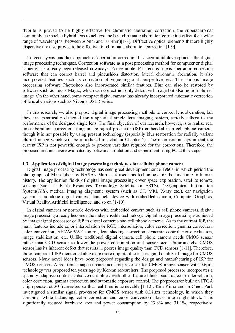
sensors. Note that the semi-diagonal corresponds to the half maximum field angle (HMFA) for all

three cases. However, HMFA is only 21 degree in Fig.1.4 due to software limitation. This will be

explained in Chapter 5.


17

Fig.1.2 Image sensor used in distortion correction

Fig.1.3 Image sensor used in chromatic aberration correction

18

Fig.1.4 Image sensor used in radially variant blur restoration

It should be emphasized that EFL, BFL and FNo. in Tab.1.1 are measured and calculated in terms

of d line of Fraunhofer Lines light beams, whose wavelength is 587.6nm. It is therefore the reference

ray for further analysis of our single lens system throughout this research. Other wavelengths will

slightly modify those values. Additionally, the object distance is regarded as infinite.

It is necessary to explain how the lens parameters in Tab.1.1 are determined. The ED, CT, EFL,

BFL, 𝑅1 and glass material in Tab.1.1 are determined by referring up to date commercial lens

catalogue and selected the parameters that are most suitable for future cell phone camera size. The

reason of choosing SF5 rather than BK7 is that the former possesses higher refractive index that is

easier to bend light beams than the latter, which can shorten the distance between foci and lens, hence

shorten the overall height of the imaging system. FNo.in Tab.1.1 is determined by the following

equation

𝐹𝑁𝑜.=𝐸𝐹𝐿

𝐸𝐷 (1.1)

The determination of half maximum field angle can be divided into two steps:

Step 1. Calculate maximum field angle using paraxial equation for infinite object

𝑦 ′̅ = 𝑓′tanω (1.2)

where 𝑦 ′̅ indicates paraxial image height, 𝑓′ is the effective focal length (EFL) and ω is the half

field angle. The equation with respect to half maximum field angle can then be derived from (1.2)

𝑦 ′̅max

= 𝑓′tan 𝜔max (1.3)

where in this case 𝑦 ′̅max

equals half of the diagonal of the image plane.

In our case,

𝜔max = arctan (𝑦 ′̅max

𝑓′) = (

2.9

3) = 44.03 degree

Step 2. Determine real maximum field angle by examining if the output image fit to the size of

image sensor perfectly.


19

Although the maximum field angle for paraxial case has been calculated, the real maximum field

angle should not equal to this because the accuracy of the paraxial equation (1.2) will fall dramatically

as the field angle increases. As a result, the output image will not fit to the image sensor perfectly.

(For example, the semi-diagonal is 2.58mm and the pixel size is 4.75μm× 4.75μm for the chromatic

aberration correction if we use 44.03 degree as the maximum field angle.) Therefore, we increased

the half field angle and found that when the angle increases to 48 degree, the output image size and

the image sensor size will perfectly match.

On the other hand, these requirements of specification for future cell phone camera are actually

contradictory because decreasing the thickness of the lens system will lead to larger maximum field

angle, which consequently increases optical aberrations. This can be proved via equation (1.3) and the

property of single lens. From equation (1.3) we could tell that increasing maximum field angle will

lead to shorter EFL, which means the thickness of the lens system is reduced. However, this is where

the problem begins. According to property of single lens, the optical aberrations will increase as the

field angle increases. And most importantly, the paraxial aberrations and the famous third order Seidel

aberrations are no longer applicable in terms of large field angle. In other words, we could not use

paraxial aberration equations or third order Seidel aberration equations to correct optical aberrations

any more. This is easy to understand because the paraxial aberrations and Seidel aberrations are all

derived by approximating Snell’s Law (𝑛 𝑠𝑖𝑛 𝜃 = 𝑛′ 𝑠𝑖𝑛 𝜃′), the difference lays in that the former is a

first order approximation ( 𝑛 𝜃 = 𝑛′𝜃′ ) and the latter uses more accurate third order

approximation 𝑛(𝜃 − 𝜃3 3!⁄ ) = 𝑛′(𝜃′ − 𝜃′33!⁄ ).We can examine the deviations of the first order

approximation and the third order approximation from the sinusoidal function for different angles in

Tab.1.2. Obviously, larger angle results in greater deviations. The deviation of the third order

approximation is smaller than that of the first order approximation.

Tab.1.2 Sinusoidal function and its first order and third order approximations

𝜃(degree) 𝑠𝑖𝑛 𝜃 𝜃(rad) 𝜃 − 𝜃3 3!⁄

1 0.0175 0.0175 0.0175

3 0.0523 0.0524 0.0523

5 0.0872 0.0873 0.0872

10 0.1736 0.1745 0.1736

15 0.2588 0.2618 0.2588

20 0.3420 0.3491 0.3420

30 0.5000 0.5236 0.4997

50 0.7660 0.8727 0.7619

Because of the above reason, the calculation results of paraxial aberration and third order aberration

will deviate too much from the real aberration value of the lens system in case of large field angle,

which increases the difficulty of aberration correction problem. To deal with the problem, we have to

modify the first order and third order aberration equations to make them applicable to large field angle.

In Chapter 3 and 4 we introduce an improved distortion term of the third order Seidel aberration

equation using field-dependent coefficient for distortion correction and an improved first order

equation for lateral chromatic aberration correction, respectively.

Therefore, the objectives of distortion correction and chromatic aberration correction are to find out

higher order equations that can accurately represent real aberration values, which will be far more

20

accurate than values calculated by traditional paraxial and third order Seidel equations so as to obtain

satisfactory results both visually and quantitatively. On the other hand, the objective of radially variant

blur restoration is to investigate a polar domain locally invariant PSF restoration method that can

simplify the matrix manipulation between image and PSF. In the following chapters, the proposed

algorithms for the three aberration correction tasks will be introduced and evaluated in detail.

1.5 Originality of this research

As we already introduced in section 1.1, there are several approaches to realize future cell phone

camera system that is not only in small dimension, requires low power consumption, but also

incorporates optical zooming and AF features. However, there is no such literature that depicts a

single lens imaging system in camera, not even in conventional digital camera, because it is well

known that this system can introduce significant optical aberrations. Therefore, it is very meaningful

to propose an optional approach for future cell phone camera, design such a system and investigate

original methods exclusively for single lens system to solve the aberration correction problems.

Therefore, the originality of this research can be concluded as follows:

1) Single lens structure

Current and most of the proposed future cell phone camera include more than one lens element to

correct aberrations optically, even though they use liquid lens or aspheric lens etc. to reduce

overall thickness. The proposed system, however, use one element of spherical double convex

single lens and no additional lens are required.

2) Improvement of traditional third order Seidel aberration equation and paraxial chromatic

aberration equation

Unlike compound lens system, the single lens system will produce intensive aberrations,

especially at high field angle. The difficulty of aberration correction for single lens requires

improvement of current aberration equations. Since the maximum field angle of the lens system

reaches 96 degree, Seidel third-order aberration equation is not able to accurately represent real

distortion value. We found that the relationship between distortion coefficient and paraxial image

height can be better represented by a third order polynomial equation. The paraxial image height is

also a function of field angle. So the field angle dependent distortion coefficient method was

devised. The other method proposed is the backward mapping method, which is directly

influenced by the obtained field angle dependent coefficient polynomial.

As to the chromatic aberration correction, the maximum field angle is also 96 degree, the

traditional paraxial chromatic aberration equation (or first order equation) is not applicable in this

case. It is found that the distance from the intersection point of chief ray and first lens surface to

the optical axis can be considered as a function of real image height. Therefore, we improved the

first order equation and found that the relationship between them can be better represented by

third order polynomial.

3) Deconvolution between polar blurred image and polar PSF for the restoration of radially variant

blurred image produced by the single lens system

Researchers have already studied one kind of radial blur caused by moving the camera

perpendicular to the object, but few have studied on the radial blur caused by inherent defect of a

single lens system. Because of the special distribution of blur: a radially variant blur produced by

spherical single lens, we considered a new method of blur restoration. Compared to traditional


21

method that deconvolves blurred image and PSF in Cartesian coordinate, the proposed method

carries out deconvolution using polar blurred image and polar PSF. The proposed method can

simplify matrix manipulation between image and PSF due to the use of locally invariant PSFs.

Finally, it should be emphasized that the current system requires further development such as

incorporating optical zooming feature. In addition, the current research has already proved to be

successful at the simulation stage, which will be introduced in the following chapters. It is expected

that the proposed methods can be implemented on a real-time ISP of cell phone in the future.

1.6 References

[1-1] K. Tatsuno, “Current trends in digital cameras and camera-phones”, Sci. Tech. Trends - Q.

Rev.18 (1) 35–44 (2006) Original Japanese version published in July 2005.

[1-2] Kuiper, S. & Hendriks, B. H. W. “Variable-focus liquid lens for miniature cameras”, Appl.

Phys.Lett. 85, 1128–1130 (2004)

[1-3] W.S. Wang, J. Fang, K. Varahramyan, “Compact variable-focusing microlens with integrated

thermal actuator and sensor”, IEEE Photon. Technol.Lett. 17, 2643–2645 (2005)

[1-4] B.Y.Song, D.S. Nam, “ Auto-focusing actuator and camera module including flexible diaphragm

for mobile phone camera and wireless capsule endoscope”, Special Issue on 18th ASME

Annual Conference on Information Storage and Processing Systems, Santa Clara, CA, USA,

16–17 June (2008)

[1-5] S. Ozawa, T. Yuasa, R. Yoshida, K. Matsusasa, “Development of an ultra-compact zoom lens

unit for camera phones”, KONICA MINOLTA TECHNOLOGY REPORT, VOL.478–81(2007)

(In Japanese)

[1-6] S. Ooshima, T. Tanaka, “Hikyumen renzu Gijutsu”, television gakaishi vol.42, No.9, 937-944

(1988) (In Japanese)

[1-7] Kishikawa T. “Kougaku Nyumon”, Optronics Press; (1990) (in Japanese)

[1-8] M. Zając, J. Nowak, “Correction of chromatic aberration in hybrid objectives, Optik”, vol. 113

299-203 (2002)

[1-9] A. Pe’er, D. Wang, A. W. Lohmann, and A. A. Firesem, “Apochromatic optical correlation,” Opt.

Lett. 25, 776–778 (2000).

[1-10] M. Takagi, H. Shimoda, “Handbook of Image Analysis”, University of Tokyo Press, Tokyo,

(1991)(in Japanese)

[1-11] K. Kim, In-Cheol Park, “Combined image signal processing for CMOS image sensor”, IEEE

International Symposium on Circuits and Systems, 2006. ISCAS 2006. Proceedings(2006)

[1-12] Y. Ho Jung, J. Seok Kim, B. Soo Hur, A. Moon Gi Kang, “Design of real-time image

enhancement preprocessor for CMOS image sensor”, IEEE Transactions on Consumer

Electronics 46 (1), 68–75(2000)

http://ieeexplore.ieee.org/search/searchresult.jsp?searchWithin=Authors:.QT.Kimo%20Kim.QT.&newsearch=partialPref

http://ieeexplore.ieee.org/search/searchresult.jsp?searchWithin=Authors:.QT.In-Cheol%20Park.QT.&newsearch=partialPref

http://ieeexplore.ieee.org/xpl/mostRecentIssue.jsp?punumber=11145

23

Chapter 2 Comparison of conventional and new

optical imaging systems

24

Chapter2 Comparison between conventional and new

optical imaging systems

2.1 Introduction

In Chapter 2, the merit and demerit of the newly proposed single lens imaging system will be

depicted and compared with the conventional compound lens imaging system. Firstly, we illustrate

some patent lens systems that use compound lens structure and specify their overall thickness and

maximum field angle. In comparison, we also give some single lens system with double convex or

plano-convex single lens element that is selected from up-to-date commercial lens catalogue in order

to show theoretically how slim the proposed single lens system could be made. Secondly, in order to

show how strong the aberration of single lens systems compared to compound lens systems, the

aberration of both systems will be illustrated and compared quantitatively by using aberration curves

and visually by PSF distribution image and 2D image simulations. Finally, we give some simulation

results using our proposed aberration correction methods by digital image processing to indicate the

feasibility to compensate for single lens aberrations, even if the conventional optical method is not

used.

2.2 Structure comparison between conventional and newly proposed optical imaging system

This section compares structures of many types of patent compound lens systems used in digital

cameras with the newly proposed single lens systems.

First of all, three compound lens systems are selected. The lens structures 2D plot using CODE V

are illustrated in Fig.2.1 to Fig.2.3 and their specifications are shown from Tab.2.1. to Tab.2.3. The

object distance is considered infinite for each of the three systems. The red, green, blue (and also

brown for Fig.2.3) lines in Fig.2.1 to Fig.2.3 indicate light beams coming from point light sources on

the object with increased field angles. For example, the red lines indicate light beams coming from a

point light source on the optical axis (field angle is 0 degree). In Tab.2.1 to Tab.2.3, we observe 3

parameters: 1) the number of optical elements, 2) overall thickness from center of the first lens front

surface to the image plane and 3) the maximum field angle.

Chapter 2 Comparison between conventional and new optical imaging systems

25

Compound lens system 1: USA patent 2559875 HERZBERGE

Fig.2.1 Structure of compound lens system (USA patent 2559875 HERZBERGE)

Tab.2.1 Specifications of compound lens system(USA patent 2559875 HERZBERGE)

No.of lens elements 5

Overall thickness (mm) (from center of the first lens front surface to image plane) 117

Maximum field angle (degree) 60

16:31:26

USA PATENT 2559875 HERZBERGE Scale: 120.00 ORA 23-Sep-10

0.21 MM

26

Compound lens system 2: USA Patent 2518719 M.REISS

Fig.2.2 Structure of compound lens system (USA patent 2518719 M.REISS)

Tab.2.2 Specifications of compound lens system (USA patent 2518719 M.REISS)




17:55:30

USA PATENT 2518719 M.REISS Scale: 90.00 ORA 23-Sep-10

0.28 MM


27

Compound lens system 3: USA Patent 4892398 90690 KUDO

Fig.2.3 Structure of compound lens system (USA patent 4892398 90690 KUDO)

Tab.2.3 Specifications of compound lens system (USA patent 4892398 90690 KUDO)




Then, we give some single lens structures that are double-convex or plano-convex in Fig.2.4 to 2.6,

in order to compare with the compound lens system structures. The selection criterion for single lens

is: low central thickness (CT), low effective focal length (EFL) and should be available on the newest

commercial lens catalogue. The purpose of the single lens system design is to realize competitively

low overall thickness and high field angle. The object distance is also considered infinite. In Tab.2.4

to Tab.2.6, we list 9 parameters: 1) overall thickness from center of the single lens front surface to the

image plane; 2) the maximum field angle; 3) glass material with its refractive index in terms of

587.6nm light beams (The reason to show the glass material is that it greatly affects the EFL of single

lens, hence the overall thickness of the imaging system.);4) Effective focal length or EFL; 5) Back

focal length or BFL; 6) Lens diameter;7) Central Thickness (CT); 8) Entrance pupil diameter and 9) F

No. .

18:24:32

USA PATENT 4892398 90690 KUDO Scale: 1.20 ORA 23-Sep-10

20.83 MM

28

Single lens system 1:

Fig.2.4 Structure of the single lens system with double convex surfaces

Tab.2.4 Specifications of the single lens system

Overall thickness (mm) (from center of the single lens front surface to image plane) 4.5


Glass material (Refractive index) SF5(1.673)

Effective focal length or EFL(mm) 3.00

Back focal length or BFL(mm) 2.21

Lens diameter(mm) 3.0

Central Thickness (CT) 2.3

Entrance pupil diameter (mm) 0.94

F No. 3.2

00:40:09

Single lens double convex Scale: 22.00 24-Sep-10

1.14 MM


29


Fig.2.5 Structure of the single lens system with plano convex surfaces


Overall thickness (mm) (from center of the single lens front surface to image plane) 1.4


Glass material(Refractive index) LaSF9(1.850)


Back focal length or BFL (mm) 0.57



Entrance pupil diameter (mm) 0.1

F No. 10.0

22:48:29

Single lens system plano convex 1 Scale: 67.00 26-Sep-10

0.37 MM

30


Fig.2.6 Structure of the single lens system with plano convex surfaces


Overall thickness (mm) (from center of the single lens front surface to image

plane)

1.0


Glass material(Refractive index) LaSF9(1.850)


Back focal length or BFL(mm) 0.17



Entrance pupil (mm) 0.1

F No. 6.0

It is evident by observing Fig.2.1 to Fig.2.3 and Tab.2.1 to Tab.2.3 that the patent lenses all

showed satisfactory aberration correction capability by using compound lens, which can be observed

from the foci of the low and high field angle light beams on the image plane (They are not positioned

in front of or in the back of the image plane). The maximum number of optical elements is 5 and the

minimum is 3. Additionally, they all showed high field angle capability: the largest reaches 80° for

the USA patent lens 2518719 M.REISS shown in Fig.2.2 and the smallest value 60° are obtained by

US patent lens shown in Fig.2.1 and Fig.2.3. However, the overall thickness from center of the first

lens front surface to image plane is extremely long: the maximum distance reaches 119mm for the

USA patent lens 2518719 M.REISS. In comparison to these compound lens systems, our newly

proposed single lens systems showed competitive overall thickness and maximum field angle. In

Fig.2.4, the overall thickness of the double convex system is 4.5mm, which is achieved by using glass

22:51:39

Single lens system plano convex 2 Scale: 100.00 26-Sep-10

0.25 MM


31

material with relatively high refractive index: SF5 and low CT (2.3mm). The EFL and BFL for this

system are 3.00mm and 2.21mm, respectively. According to Fig.2.5 and Fig.2.6, the overall thickness

could be further shortened by using plano-convex surfaces and higher refractive index glass LaSF9.

The overall thickness is obtained by adding BFL and CT of the lens. Ultra-thin thickness of the lens

system is achieved for plano-convex lens 1 (1.4mm) and plano-convex lens 2(1.0mm). The high field

angle range (0~96 degree) is still obtainable by sacrificing the diameter of entrance pupil. The central

area around the optical axis showed no spherical aberrations because the entrance pupil is relatively

very small compared to lens diameter. Therefore sharp image could be formed around image center.

However, the other aberrations such as distortion, field curvature and lateral chromatic aberration

(LCA) are very strong compared to compound lens aberrations and become extremely strong when

the field angle reaches highest value. For example, the field curvature can be observed by the foci of

low and high field angle light beams: the light beams coming from the off axis point source failed to

focus on the image plane but in front of it and the higher the field angle the longer the distance

between foci and image plane. This phenomenon results in an image with increased blur pattern from

image center. In the next section, comparison of aberrations between the compound lens systems and

the single lens systems will be illustrated quantitatively in aberration curves and visually in PSF

distribution image and 2D image simulation.

2.3 Comparison of optical aberrations between conventional and newly proposed optical

imaging system

Firstly, we give the following curves showing distortion and lateral chromatic aberration (LCA) for

the three compound lens systems and the three single lens systems. Distortion will lead to geometrical

deformation from the normal image and LCA results in displacement between different colors on the

image plane. These two aberrations are not related to image blur. Other optical aberrations: spherical

aberration, coma, astigmatism, field curvature and axial chromatic aberration (ACA) all result in blur

on the image plane, so that they can be represented by PSF distribution images shown in Fig.2.10.

The values are calculated by real ray tracing, so that it is neither first order values nor third order

Seidel aberration values. In order to unify the maximum field angle for comparison, we only measure

distortion and LCA that belongs to half field angle lower than 30 degree for all the six imaging

systems.

The distortion values are measured in terms of the reference light beams whose wavelength is

587.6nm. In Fig.2.7, the horizontal axis shows semi field angle (or half field angle) and the vertical

axis shows the distortion in percentage. The distortion is calculated by obtaining the difference

between real chief ray height and paraxial chief ray height on the image plane and then divided by the

paraxial chief ray height. Suppose the paraxial chief ray height is 𝑦 ′̅ and the real chief ray height is

𝑦′, then we have

' '

100%'

y ydist

y

(2.1)

It can be observed from Fig.2.7 that distortion values of the compound lens systems are much

smaller than that of the single lens systems. The maximum distortion among compound lens systems

is approximately -1.9%, while the minimum distortion among single lens system already surpasses

this value, reaching up to approximately -4.3%. The maximum distortion -8.2% for single lens

systems is obtained by single lens 1 at field angle 30 degree. As the field angle increases, the

distortion will further increase as well. We have measured that the distortion value rises up to -23.0%

at the maximum semi field angle 48 degree for the double convex single lens system, which is very

large for an imaging system.

32

Fig.2.7 Comparison of distortion among compound lens systems and single lens systems

Similarly, the graphs showing LCA for the three compound lens systems and the three single lens

systems are illustrated in Fig.2.8 and Fig.2.9. The LCA values are measured between chief rays of

Fraunhofer F line (486.1nm) and C line (656.3nm) light beams, and between chief rays of F line and d

line (587.6nm) light beams. Therefore, two graphs are drawn separately. The horizontal axis is the

semi field angle and the vertical axis indicates LCA values in millimeters. The LCA between F line

and C line light beams are larger than that between F line and d line light beams for all the six systems

because the wavelength difference of the former is relatively larger than the latter. Except the

compound lens 3, the other two compound lens systems all showed smaller LCA values than the

single lens systems. The curves depicting compound lens 1 and compound lens 2 almost overlapped

with each other, showing LCA values very close to zero. The maximum LCA: -0.2μm and -0.1μm is

obtained at semi field angle 30 degree for compound lens 2. As an exception, the LCA values of

compound lens 3 show very unstable variation: being positive when the field angle is lower than 22.5

degree and negative when it is above 22.5 degree, and the maximum LCA even exceeded that of

single lens 1, which is possible for certain kind of lens system. Besides compound lens 3, the LCA of

single lens 1 surpasses all the others, showing maximum LCA -0.017mm and -0.012mm at semi field

angle 30 degree. The LCA of single lens 2 and 3 overlapped with each other, showing near equivalent

values.

-9

-8

-7

-6

-5

-4

-3

-2

-1

00 6.59 13 19.11 24.79 30

Dis

tort

ion

(%

)

Semi field angle(degree)

Compound lens 1

Compound lens 2

Compound lens 3

Single lens 1

Single lens 2

Single lens 3


33

Fig.2.8 LCA comparison between F line and C line light beams among compound lens systems and

single lens systems

Fig.2.9 LCA comparison between F line and d line light beams among compound lens systems and

single lens systems

Finally, the Point Spread Function (PSF) distribution images that are result of all blur-forming

aberrations (coma, astigmatism, field curvature and the axial chromatic aberration) are shown in

Fig.2.10. In addition, we give the 2D image simulation results in Fig.2.11, in which a photograph of a

visually normal two dimensional image is “taken” by these lens systems. The resulting image includes

all optical aberrations mentioned above. Two test images are simulated: one with rectangular frames

in order to show distortion and LCA, the other includes small English characters in order to show

radially variant blurring effect.

-0.03

-0.025

-0.02

-0.015

-0.01

-0.005

0

0.005

0.01

0 3 6 9 12 15 18 21 24 27 30

LCA

F a

nd

C(m

m)

Semi Field angle (degree)

Compound lens 1

Compound lens 2

Compound lens 3

Single lens 1

Single lens 2

Single lens 3

-0.025

-0.02

-0.015

-0.01

-0.005

0

0.005

0 3 6 9 12 15 18 21 24 27 30

LCA

F a

nd

d (

mm

)

Semi Field angle(degree)

Compound lens 1

Compound lens 2

Compound lens 3

Single lens 1

Single lens 2

Single lens 3

34

(a) Compound lens 1 (b) Compound lens 2 (c) Compound lens 3

(d) Single lens 1 (e) Single lens 2 (f) Single lens 3

Fig. 2.10 PSF distribution of the compound lens systems and the single lens systems

(a) (b) (c) (d) (e) (f) (g)

(h) (i) (j) (k)


35

(l) (m) (n) (o)

(p) (q) (r) (s)

Fig.2.11 2D image simulation results of test image 1 for the compound lens systems and the

single lens systems: (a) original image; (b) (c) (d) (e) (f) (g) image produced by compound lens

system 1, 2, 3 and single lens system 1,2,3, respectively; (h) (i) zoom in of area 1 and 2 for

compound lens system 1; (j) (k) zoom in of area 1 and 2 for compound lens system 2; (l) (m) zoom

in of area 1 and 2 for compound lens system 3; (n) (o) zoom in of area 1 and 2 for single lens system

1; (p) (q) zoom in of area 1 and 2 for single lens system 2; (r) (s) zoom in of area 1 and 2 for single

lens system 3.

(a) (b) (c) (d)

(e) (f) (g)

Fig.2.12 2D image simulation results of test image 2 for the compound lens systems and the

single lens systems: (a) original image; (b) (c) (d) (e) (f) (g) image produced by compound lens

system 1,2,3 and single lens system 1,2,3, respectively.

36

The PSF distribution images shown in Fig.2.10 demonstrate that all compound lens systems

produce sharp point images for low and high field angle regions. Nevertheless, the PSFs of single lens

systems indicate radially increasing blur effect from image center to image borders, which is a result

of field curvature phenomenon that is already explained in Section 2.2. The PSFs at high field angles

are more intensive for the spherical double convex system shown in Fig.2.10 (d) than the two

plano-convex systems shown in Fig.2.10 (e) and (f), indicating that fewer aberrations can be obtained

by using plano-convex system. This can also be confirmed in the 2D image simulation results in Fig.

2.12.

2D simulation on test image 1 shown in Fig.2.11 is to visually examine distortion and LCA of the

compound lens systems and single lens systems. According to Fig.2.11 (b) to (g), strong distortion can

be easily observed on high field regions of single lens systems, whereas distortion of compound lens

systems can barely be observed. Among the single lens systems, the strongest distortion was obtained

by (e): the double convex system. This is consistent with the result of distortion curves shown in

Fig.2.7. In order to show LCA, we enlarged areas where the LCA is relatively strong for the six

optical systems. The areas to be enlarged are marked with number “1” and “2” in Fig.2.11 (a). The

corresponding enlarged images are given from Fig.2.11 (h) to (s). As is expected, single lens systems

obtained stronger LCA than compound lens systems, which can be perceived by blue color on the

inner fringe of the rectangular frames. The strongest LCA among single lens systems belongs to the

double convex lens, which can also be observed from LCA curves shown in Fig.2.8 and Fig.2.9.

2D simulation on test image 2 shown in Fig.2.12 is to visually examine radially variant blur effect

of the single lens systems. Obviously, the resulting images of the compound lens systems showed

little blur effect compared with those of the single lens systems. Among all the single lens systems,

although the low field regions are visually normal, the high field regions are strongly blurred and

distorted, which is understandable with the help of PSF distribution images in Fig.2.10.

2.4 The feasibility to compensate for single lens aberrations using digital image processing

techniques

This section demonstrates the feasibility of correcting aberrations for single lens system using the

proposed image digital processing methods rather than using the compound lens. As the detailed

description of results will be given on the following chapters, we only show briefly the resulting

images. The simulation of aberration correction is carried out based on the aberration values of the

double convex single lens, the plano-convex systems will not be addressed here.

The resulting images of distortion correction and LCA correction for test image 1 are shown in

Fig.2.13 to Fig.2.15.

(a)distorted (b) distortion corrected

Fig.2.13 Comparison between distorted image and corrected image


37

(a) before LCA correction (b) LCA corrected

Fig.2.14 Image comparison before and after LCA correction for region 1

(c) before LCA correction (d) LCA corrected


As to the restoration of radially blurred image, we set the maximum field angle to 21 degree

because of the software limitation, which says the PSF will become inaccurate when the field angle is

larger than 21 degree. This will be further discussed in Chapter 5.

Image restorations of two monochromatic images are shown in Fig.2.16.

(a) blurred (b) restored (c)blurred (d)restored

Fig.2.16 Radially blurred image restoration for two monochromatic images

2.5 Conclusion

In conclusion, this chapter compared the structure of three compound lens systems and three single

lens systems and showed that the overall thickness from center of the first lens front surface to image

plane can be reduced to approximately 1.0mm by using plano-convex single lens whereas this

distance of the current cell phone cameras are 7~10mm. The maximum field angle (MFA) can be

increased to 96 degree if the entrance pupil diameter is relatively small compared to lens diameter. In

spite of a special case such as compound lens system 3, distortion and LCA curves indicated that the

distortion and LCA values of single lens systems all exceeded that of the compound lens systems. PSF

38

distribution images and 2D image simulation results showed more intensive radial blur effect at high

field angle regions for single lens systems than compound lens systems. The resulting images for

distortion, LCA correction and image restoration demonstrated that optical aberrations produced by

single lens systems can be minimized by digital image processing techniques, even if optical means is

not used.

Finally, a table showing merit and demerit of compound lens systems and single lens systems is as

follows:

Tab.2.7 Merit and demerit of two lens systems

Conventional compound lens system Proposed single lens system

Merit Few optical aberrations by optical

correction

Thinner and slimmer

Demerit Overall thickness is very long Significant optical aberrations

(But can be minimized by

digital image processing

techniques)


39

40

Chapter 3 Correction of distortion


41


3.1 Introduction

This chapter introduces distortion correction methods for single lens systems. Before introducing

our methods, it is necessary to briefly present the research background of this field of study. In the

literatures of geometrical distortion correction, researchers have proposed many algorithms aiming at

compensating for lens distortion digitally. For example, polynomial warping correction method is

known as the most widely used distortion correction method, in which a polynomial equation of

degree N is determined by a set of control points in the first step. Then the polynomial equation

coefficients were calculated from the control points by least-squares minimization. Finally, use the

polynomial equation to transfer the points from the distorted image to a corrected image [3-1].

Another simple mathematical model for lens distortion correction was introduced by H. Ojanen [3-2],

which is applicable to three types of lens distortion: barrel distortion, pincushion distortion and the

combination of the two basic types. The correction was done by building up a composite mapping

function between the object plane and the film plane, taking consideration not only the undistortion

function but also other functions that are needed to compensate for inaccuracies in the test setup and

using least-squares method to choose the undistortion parameters. On the other hand, some algorithms

are dedicated to applying to specific imaging systems. For instance, field mapping and point spread

function (PSF) mapping were proposed and compared to correct intensity distortion and geometrical

distortion in Echo-planar imaging (EPI) system [3-3] and a geometrical distortion correction method

based on image normalization was introduced by M.Alghoniemy, which can be applied to image

watermarking systems that are vulnerable to geometric attacks [3-4]. Methodologies for barrel

distortion correction in electronic endoscope images suggest that the non-linear inhomogeneous

distorted images due to wide-angle configuration of the camera lens can be corrected by building up a

correction model and estimating the correction parameters [3-5],[3-6].

Additionally, as an indispensable process after our integer mapping method that will be introduced

in the following sections, interpolation plays a crucial role in determination of the values of pixel

vacancies and restoring the pixel continuity of the distortion-corrected image. Therefore, a brief

review on the development of interpolation methods is very helpful to understand our texture

dependent interpolation method proposed in [3-17]. Many interpolation techniques have been

proposed by predecessors in this field of research. The well-known and most commonly used should

be the polynomial interpolation, in which case the basic idea is to represent an unknown pixel value

by a polynomial, solving polynomial equation set to obtain the coefficients of polynomial. Then

compute the unknown pixel value by substituting the vertical and horizontal coordinates into the

polynomial equation. The number of coefficients should be equal to that of the polynomial equations,

in other words, to the number of neighboring pixels that are used to calculate coefficients. Application

of polynomial interpolation other than image processing was also introduced to estimate heights of a

continuous surface for the DEM (Digital Elevation Model) [3-7]. In the literature of linear and

space-invariant interpolation, the commonest interpolation methods are nearest neighbor interpolation,

bilinear interpolation and bicubic interpolation, whose mathematical expressions can be derived by

adding or reducing the number of coefficients of the polynomial equation. In the Video and Image

Processing Blockset of Matlab, nearest neighbor interpolation is implemented by obtaining nearby

translated pixel values, bilinear interpolation is implemented by obtaining weighted average of the

two translated pixel values on either side of the input pixel. Bicubic interpolation is implemented

similarly by obtaining weighted average of the four translated pixel values on either side of the input

pixel. Another algorithm depicted that the bilinear interpolation creates new pixels based on color

averages from both the horizontal and vertical neighbors of the area to be resized, and the bicubic

interpolation creates new pixels based upon weighted average from horizontal, vertical and diagonal

directions. Much smoother images can be obtained by Cubic Splines or B-splines, which was first

42

introduced by H.C.Andrews and C.L.Patterson in 1976[3-8] and a detailed mathematical analysis was

proposed by H.S.Hou and H.C. Andrews in 1978[3-9]. There are other superior interpolation schemes

such as isophote-oriented methods, which usually employ a PDE (Partial Differential Equation)

iterative interpolation, mainly proposed to avoid zigzagging artifacts around edge introduced by

traditional linear interpolation methods[3-10] to [3-13]. Comparison among different interpolation

methods [3-14] and [3-15] were documented to provide a comprehensive reference by which we are

able to pick up an optimal method for a specific application.

In this chapter, the original method “Field angle dependent distortion coefficient” will be described

firstly. This method was proposed because the distortion component of the traditional third order

Seidel aberration is not accurate to represent real distortion values in case of high field angles. For

example, the double convex single lens system depicted in Chapter 2 results in 0.3710mm deviation

from the real distortion value at half field angle 48 degree if third order distortion component is

utilized. Therefore, improvement should be made to the third order distortion component in order to

correct distortion precisely. Secondly, forward mapping and backward mapping methods will be

introduced and compared. The former obtains the distortion-corrected image from the distorted image

while the latter maps image pixels from a virtual distortion-free, ideal image to a distorted image. The

latter is superior to the former because of two reasons: 1) no pixel vacancies will be created after

distortion, thus the additional interpolation process is unnecessary; 2) higher precision of pixel values

is obtainable because bilinear interpolation is employed rather than nearest neighbor interpolation

used in forward mapping method. Finally, simulation results of the proposed techniques of distortion

correction will be discussed.

3.2 Methods

3.2.1 Distortion coefficient depending on field angles

The algorithm to correct distortion is based on the famous third order Seidel aberration theory but

with some improvement because the maximum field angle in our lens design is very high. The Seidel

third order aberration approximates the Snell’s Law 𝑛 𝑠𝑖𝑛 𝜃 = 𝑛′ 𝑠𝑖𝑛 𝜃′ to 𝑛(𝜃 − 𝜃3 3!⁄ ) =

𝑛′(𝜃′ − 𝜃′33!⁄ ), therefore higher precision can be obtained when we calculate optical aberrations

than the paraxial approximation 𝑛𝜃 = 𝑛′𝜃′.

The distortion component of the third order Seidel aberration equation can be expressed as follows

[3-16]

3' 'disty S y

(3.1)

The real distortion occurring on the image plane can be expressed as

'

_ ' 'dist realy y y (3.2)

The third order distortion approximately equals to the real distortion when the field angle is not too

high, which can be written as follows 3

' ' 'S y y y (3.3)

In equations (3.1) to (3.3), Δ𝑦𝑑𝑖𝑠𝑡′ and Δ𝑦𝑑𝑖𝑠𝑡_𝑟𝑒𝑎𝑙

′ mean third order distortion and real distortion,

respectively. 𝑦 ′̅means the ideal image height and 𝑦′is real image height, which is distorted from the

ideal image height �̅�′. S indicates distortion coefficient. When the field angle is very high, equation

(3.3) has to be modified, otherwise the accuracy of the third order distortion will decline dramatically

and no longer equals to right side of the equation. To precisely represent the distortion value at every

field angle, we regard distortion coefficient S as a continuously changing value rather than a constant.

In other words, S should be considered as a function of 𝑦 ′̅, or 𝑆 = 𝑓(𝑦 ′̅). We found that the relation

between 𝑆 and �̅�′ can be better represented by polynomial approximation than other curve

approximation. Therefore, we calculated 𝑆 by rewriting equation (3.3) for different field angles as


43

different sample points using the real distortion Δ𝑦𝑑𝑖𝑠𝑡_𝑟𝑒𝑎𝑙′ and ideal image height 𝑦 ′̅.

'

_

3

'

dist realyS

y

(3.4)

In this equation, the values of real distortion Δ𝑦𝑑𝑖𝑠𝑡_𝑟𝑒𝑎𝑙′ can be directly read out by optical design

software CODE V when the single lens system is built up. And the ideal image height 𝑦 ′̅ can be

calculated by equation (3.5). '' tany f (3.5)

This equation is known as the paraxial equation that calculates the image height when the object

distance is infinite. 𝜔 is the half field angle, 𝑓′ indicates Effective Focal Length(EFL) and 𝑦 ′̅ means paraxial image height (also ideal image height).

Take the double convex single lens for example, when the half field angle reaches maximum (48

degree), 𝑦 ′̅ is 3.332mm. The value of real distortion Δ𝑦𝑑𝑖𝑠𝑡_𝑟𝑒𝑎𝑙′ is -0.7682mm. Therefore S is

-0.0208(1/mm2). Then we made a third order polynomial approximation between S and 𝑦 ′̅. By

doing this we can calculate S for all field angles, not only the sample points. The sample data,

relationship curve and the corresponding third order polynomial equation will be given in Section 3.3.

3.2.2 Comparison between forward and backward mapping methods.

1) Forward mapping method:

The forward mapping method, as its name suggests, maps image pixels from a distorted image to

an ideal distortion-free image. It can be further divided into integer pixel mapping and decimal pixel

mapping methods. Fig.3.1 illustrates the schema of the two forward mapping methods:

(a) Integer pixel mapping

(b) Decimal pixel mapping

Fig.3.1 Schema of the forward mapping method

The solid dot in Fig.3.1 means pixel of the original distorted image and the mapped pixel in the

corrected image. The hollow dot means pixel vacancy that is created by using forward mapping

method. Fig.3.1(a) shows that an integer pixel in the original distorted image is mapped to the

corresponding position in a corrected image. However, pixel vacancies appear around the mapped

44

pixel. Therefore data interpolation has to be employed to fill up those vacancies. We proposed a

texture dependent interpolation method [3-17] that determines the value of a pixel vacancy by texture

around the pixel. This interpolation can be classified into 16 cases and the pixel value is obtained by

nearest neighbor, linear interpolation or bilinear interpolation according to specific cases. The decimal

pixel mapping method shown in Fig.3.1 (b), however, does not create vacancies if sufficient decimal

pixels are defined around the integer pixel in the original distorted image. In other words, the hollow

dots shown in Fig.3.1 (a) have their corresponding positions that are provided by decimal pixels. In

the following paragraphs, we will introduce the two methods in details.

The equation that determines the pixel position on a distortion-free ideal image for both integer

mapping and decimal mapping can be expressed as follows:

''

' '31

yy

S y

(3.6)

This equation is a modified version of equation (3.3). The reason to modify (3.3) is that usually we

only have a geometrically distorted image in hand and hope to know the value of ideal image height

𝑦 ′̅ from the distorted image height 𝑦′, that is, 𝑦 ′̅ = 𝑓( 𝑦′). However, according to equation (3.3) we

know that obtaining 𝑦′ ̅̅̅̅ from 𝑦′ is not an easy task as we have to deal with the cubic root. Therefore,

we rewrote (3.3) to 𝑆′𝑦′3𝑦 ′̅ = 𝑦′ − 𝑦 ′̅ and further to 𝑆′𝑦′

3= ( 𝑦′ − 𝑦 ′̅)/𝑦 ′̅ to avoid dealing with

cubic root so that simplified the forward mapping equation to 𝑦 ′̅ = 𝑦′/(1 + 𝑆′𝑦′3) . Here

𝑆′𝑦′3= ( 𝑦′ − 𝑦 ′̅)/𝑦 ′̅ also represents third order distortion value in percentage. Note that 𝑆′ does

not mean the third order distortion coefficient of Seidel aberration anymore. In our previous study

[3-17] to [3-20], we did not consider the lens design process, only showed how the geometrically

distorted image can be corrected by correction algorithm, where 𝑆′ in the modified equation can be

easily determined by visually measuring the distorted image. If we take account of the lens design

process, the equation 𝑆′𝑦′3= ( 𝑦′ − 𝑦 ′̅)/𝑦 ′̅ is not useful anymore because the third order distortion

coefficient 𝑆 has to be calculated from lens design data.

The interpolation after the integer pixel mapping process is called the texture dependent

interpolation method. This interpolation is actually a case dependent (or case analysis) method that

can be categorized into 16 cases based on the following fundamental methods:

Fig.3.2 Interpolation grid: the central pixel 𝑕9 is determined by the nearest pixels: 𝑕1 to 𝑕4 . All pixels in this grid are equally spaced.

(1) Nearest Neighbor

9 1h h or 9 2h h or 9 3h h or 9 4h h (3.7)

(2) Linear interpolation

1 39

2

h hh

or 2 4

92

h hh

or 1 2

92

h hh

or


45

2 39

2

h hh

or 3 4

92

h hh

or 4 1

92

h hh

(3.8)

(3) Bilinear Interpolation

1 2 3 49

4

h h h hh

(3.9)

The 16 cases of texture dependent interpolation can be further divided into 5 groups:

○1 Four pixels located on the vertical and horizontal neighbors are all non-zeros, in which case we

carry out bilinear interpolation using values of the four pixels (one case in all). For example, 𝑕1𝑕2𝑕3

and 𝑕4 in Fig.3.2 are all non-zero pixels, therefore we obtain the value of 𝑕9 by (3.9).

○2 Three pixels located on the vertical and horizontal neighbors are non-zeros and one zero pixel, in

which case we carry out linear interpolation using values of the two non-zero pixels that align with the

central pixel (4 cases in all). For example, only 𝑕1 in Fig.3.2 is zero pixel, therefore we obtain the

value of 𝑕9by 𝑕9 = (𝑕2 + 𝑕4)/2 of (3.8).

○3 Two pixels located on the vertical and horizontal neighbors are non-zeros and two zero pixels.

Whether the two non-zero pixels are opposite to each other, or they are next to each other, we carry

out linear interpolation using their values (6 cases in all). For example, 𝑕1 and 𝑕3 in Fig.3.2 are

non-zero pixels, then 𝑕9 can be obtained by 𝑕9 = (𝑕1 + 𝑕3)/2 of (3.8) or 𝑕1and 𝑕2 are non-zero

pixels, then 𝑕9can be obtained by 𝑕9 = (𝑕1 + 𝑕2)/2 of (3.8).

○4 One pixel located on the vertical or horizontal neighbors is non-zero and three zero pixels, in which

case we carry out nearest neighbor using value of the non-zero pixel (4 cases in all). For example, 𝑕1

in Fig.3.2 is the non-zero pixel, therefore 𝑕9 can be obtained by 𝑕9 = 𝑕1 of (3.7).

○5 There is no non-zero pixel at all (one case in all) on the vertical or horizontal neighbors, in which

case the interpolation will not be carried out. For example, 𝑕9 in Fig.3.2 will be zero if 𝑕1 to 𝑕4

are all zero pixels.

It should be emphasized that the texture dependent interpolation only takes use of the nearest four

pixels so that the pixels on the diagonal directions will not be taken into account.

To assure the proposed algorithm can interpolate any kinds of image, including those with almost

all zero valued pixels (but have few dots being non-zeros), we add 1 to all pixels before the correction

process, and subtract 1 from all pixels after the interpolation process. Doing so will avoid

misunderstanding about two kinds of zero valued pixels. The first kind of zeros belong to the original

image (before correction process), and the second kind are vacancies brought out by the correction

process, in which the original image is enlarged.

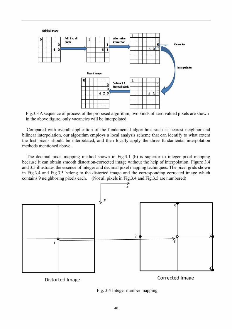
46

Fig.3.3 A sequence of process of the proposed algorithm, two kinds of zero valued pixels are shown

in the above figure, only vacancies will be interpolated.

Compared with overall application of the fundamental algorithms such as nearest neighbor and

bilinear interpolation, our algorithm employs a local analysis scheme that can identify to what extent

the lost pixels should be interpolated, and then locally apply the three fundamental interpolation

methods mentioned above.

The decimal pixel mapping method shown in Fig.3.1 (b) is superior to integer pixel mapping

because it can obtain smooth distortion-corrected image without the help of interpolation. Figure 3.4

and 3.5 illustrates the essence of integer and decimal pixel mapping techniques. The pixel grids shown

in Fig.3.4 and Fig.3.5 belong to the distorted image and the corresponding corrected image which

contains 9 neighboring pixels each. (Not all pixels in Fig.3.4 and Fig.3.5 are numbered)

Fig. 3.4 Integer number mapping

1

'2

'5

'1

'3

'4

x

y

Corrected Image Distorted Image


47

Fig. 3.5 Decimal number mapping

The solid dots in Fig.3.4 and Fig.3.5 represent pixel vacancies with zero value, that is, pixel

discontinuity caused by the expansion of the original image, while the hollow dots indicate pixels

with non-zero value. In Fig. 3.4, pixel 1( 𝑝1 in short) in a distorted image is transferred to 𝑝1′ in a

corrected image using the integer pixel mapping method. The neighboring pixels around 𝑝1′: 𝑝2′ 𝑝3′ 𝑝4′and 𝑝5′, however, have no corresponding pixels in the distorted image. In other words,

they cannot be transferred from anywhere of the distorted image but are newly created pixels with

zero value. In Fig.3.5, we define some decimal number pixels 𝑝11 𝑝21 𝑝31and 𝑝41 around 𝑝1 in

the distorted image within a range (the distance from a decimal pixel to 𝑝1 should not exceed half of

the length between two integer pixels), and they are transferred to 𝑝2′ 𝑝3′ and 𝑝4′ in the corrected

image by decimal number mapping method. Note that the same positions around 𝑝1′: 𝑝2′ 𝑝3′ and

𝑝4′, which cannot be mapped by integer pixel mapping are successfully mapped from the decimal

pixels. Therefore, we could tell that the number of vacancies in the corrected image is reduced by

virtue of the decimal pixel mapping approach.

To describe pixels in Fig.3.4 and Fig.3.5 quantitatively, we define the following mathematical

symbols:

In Fig.3.4

Distorted Image:

𝑝1: (𝑥1, 𝑦1) (3.10)

Corrected Image:

1 '1

y

x

11

21

31

41

'2 '3

'4

'5

Corrected Image Distorted Image

48

𝑝1′: (𝑥1

′ , 𝑦1′ ); 𝑝𝑣

1′= 𝑝𝑣

1

𝑝2′: (𝑥2

′ , 𝑦2′ ) = (𝑥1

′ − 1, 𝑦1′ ); 𝑝𝑣

2′= 0

𝑝3′: (𝑥3

′ , 𝑦3′ ) = (𝑥1

′ + 1, 𝑦1′ ); 𝑝𝑣

3′= 0

𝑝4′: (𝑥4

′ , 𝑦4′ ) = (𝑥1

′ + 1, 𝑦1′ + 1); 𝑝𝑣

4′= 0

𝑝5′: (𝑥5

′ , 𝑦5′ ) = (𝑥1

′ , 𝑦1′ − 1); 𝑝𝑣

5′= 0 }

(3.11)

In Fig.3.5

Distorted Image

𝑝1: (𝑥1, 𝑦1)

𝑝11: (𝑥11, 𝑦11) = (𝑥1 + 𝑎1, 𝑦1 + 𝑏1) − 0.5 ≤ 𝑎1, 𝑏1 ≤ 0.5

𝑝21: (𝑥21, 𝑦21) = (𝑥1 + 𝑎2, 𝑦1 + 𝑏2) − 0.5 ≤ 𝑎2, 𝑏2 ≤ 0.5

𝑝31: (𝑥31, 𝑦31) = (𝑥1 + 𝑎3, 𝑦1 + 𝑏3) − 0.5 ≤ 𝑎3, 𝑏3 ≤ 0.5

𝑝41: (𝑥41, 𝑦41) = (𝑥1 + 𝑎4, 𝑦1 + 𝑏4) − 0.5 ≤ 𝑎4, 𝑏4 ≤ 0.5}

(3.12)

Corrected Image

𝑝1′: (𝑥1

′ , 𝑦1′ ); 𝑝𝑣

1′= 𝑝𝑣

11 = 𝑝𝑣

1

𝑝2′: (𝑥2

′ , 𝑦2′ ) = (𝑥1

′ − 1, 𝑦1′ ); 𝑝𝑣

2′= 𝑝𝑣

21= 𝑝𝑣

1

𝑝3′: (𝑥3

′ , 𝑦3′ ) = (𝑥1

′ + 1, 𝑦1′ ); 𝑝𝑣

3′= 𝑝𝑣

31= 𝑝𝑣

1

𝑝4′: (𝑥4

′ , 𝑦4′ ) = (𝑥1

′ + 1, 𝑦1′ + 1); 𝑝𝑣

4′= 𝑝𝑣

41= 𝑝𝑣

1

𝑝5′: (𝑥5

′ , 𝑦5′ ) = (𝑥1

′ , 𝑦1′ − 1); 𝑝𝑣

5′= 0 }

(3.13)

where 𝑥1, 𝑦1 and 𝑥𝑛1, 𝑦𝑛1 denote coordinate index of pixel 𝑝1 and 𝑝𝑛1 in the distorted image,

respectively. 𝑥𝑛′ , 𝑦𝑛

′ is coordinate index of pixel 𝑝𝑛′ in the corrected image. 𝑝𝑣1, 𝑝𝑣𝑛1 and 𝑝𝑣𝑛′ indicate pixel value of 𝑝1, 𝑝𝑛1 and 𝑝𝑛′, respectively.

According to (3.12), the decimal pixels 𝑝11 𝑝21 𝑝31and 𝑝41 in Fig.3.5 are randomly generated

within the range of

1 1 1

1 1 1

0.5 0.5

0.5 0.5

n

n

x x x

y y y

(3.14)

1,2,3,4n In general, the coordinate range of the decimal pixels 𝑝𝑛𝑚(𝑥𝑛𝑚, 𝑦𝑛𝑚)around an integer pixel

𝑝𝑚(𝑥𝑚, 𝑦𝑚) in a distorted image can be defined as

0.5 0.5

0.5 0.5

m nm m

m nm m

x x x

y y y

(3.15)

where m indicates the index of an integer pixel in a distorted image, whose maximum value is

determined by the resolution of the image. n is the index of a decimal pixel around 𝑝𝑚within the

range defined by (3.15). The pixel value of all the decimal pixels 𝑝𝑣𝑛𝑚 should be equivalent to the

pixel value of the integer pixel 𝑝𝑣𝑚.

In order to avoid minus coordinates of the decimal pixels, the coordinate of the origin should not

be positioned to (0,0), (1,0) or (0,1), but to some coordinates that are greater than (1,1). Actually, we


49

positioned the origin to (101,101) by adding four black borders to the original image that are 100

pixels in width each, which will not only avoid minus coordinates but also the pixel overflow due to

the expansion of the original image in the correction process.

Another fact that should not be neglected is that not all decimal pixels can find a corresponding

mapping position in the corrected image, and some decimal pixels may overlap with other pixels as

well. Actually, there exist three kinds of mapping results by decimal pixel mapping method:

(1) Mapping positions exist in the corrected image and no overlap

This mapping frequently occurs and helps reduce the number of vacancies while the integer pixel

mapping fails to do so. For example, 𝑝21to 𝑝2′, 𝑝31to 𝑝3′and 𝑝41to 𝑝4′in Fig.3.5.

(2) Mapping positions exist in the corrected image with position overlap

This mapping also frequently occurs but do not reduce the pixel vacancies. For example, 𝑝11and

𝑝1 all mapped to 𝑝1′ in Fig.3.5.

(3) Mapping positions do not exist in the corrected image

This mapping rarely occurs compared with the other two cases. For example, 𝑝5′in Fig. 3.5

cannot find a mapping position from the distorted image.

In conclusion, the algorithm of two forward mapping methods (integer pixel and decimal pixel

mapping) all share the common property that obtains coordinates of distortion-corrected image from

the distorted image. The superiority of decimal pixel to integer pixel mapping has also been proved.

In the following paragraphs, we will introduce another distortion correction method that is superior to

both integer pixel and decimal pixel mapping methods.

2) Backward mapping method:

In contrast to the forward mapping method, the backward mapping method maps pixels from a

virtual distortion-free, ideal image to a distorted image. The equation that defines this process is

derived from expression (3.3). Rewriting (3.3), the image height in the distorted image can be

calculated by

3

' ' 'y y S y (3.16)

The flow chart and a schema of the backward mapping method are illustrated in Fig.3.6 and Fig.3.7,

respectively.

50

Fig.3.6 Flow chart of the backward mapping method

Fig.3.7 Schema of the backward mapping method

According to Fig.3.6, the first step is to create a black ideal image that has the same resolution as

the original distorted image. All pixel values are zeros at this step. Then each pixel coordinate from

the black ideal image is mapped to the original distorted image by equation (3.16), resulting in

decimal pixels (refer to Fig.3.7). The coordinates of the mapped pixels are marked in both the original

distorted image and the created black ideal image so that the corresponding positions can be easily

found. The next step is to determine pixel value of each decimal pixel by bilinear interpolation from

the surrounding four integer pixels in the original distorted image, as illustrated in Fig.3.7. The last

procedure is to locate the pixel coordinates in the black ideal image by the corresponding marked

positions and fill the black pixels with the interpolated pixel values, then output the corrected image.

3) Comparison between forward mapping and backward mapping methods:

Compared to integer pixel mapping, the backward mapping method proposed in this research will

not create any pixel vacancy after correcting distorted image, thus the extra interpolation process is no

longer needed. Compared with decimal pixel mapping, in which the interpolation is also unnecessary

if the decimal pixels defined are sufficient, the backward mapping also has advantages on the

determination of the pixel value. The decimal pixel mapping method, which is also a forward


51

mapping method, does not create black image, but directly determines pixel value of each randomly

created decimal pixel by its nearby integer pixel from the distorted image, In other words, it used a

nearest neighbor interpolation to determine each pixel value. In backward mapping method, however,

each pixel value of the black ideal image is calculated by bilinear interpolation using four integer

pixels around the mapped decimal pixel in the original distorted image. Additionally, the decimal

pixel mapping will possibly result in pixel overlapping if too many decimal pixels are defined around

an integer pixel as well as pixel loss, whereas the backward mapping will not because its one-to-one

pixel mapping mechanism.

3.3 Results and discussions.

3.3.1 Simulation environment and preparation

2D image simulation was carried out on test images and natural color image. The 2D image

simulation evaluates the resulting image of a two dimensional object (no optical aberration) using the

designed lens system. The resulting image definitely includes all the real optical aberrations, including

distortion. Then correction of distortion was carried out to evaluate the distortion correction

techniques for the designed single lens system. Before the process of distortion correction, the unit has

to be converted from millimeter to pixel because the image being corrected is measured by pixels

rather than millimeter. In our lens design, the number of pixels per millimeter can be calculated by

using single pixel size 1.4μm ×1.4μm, that is, 1/1.4μm = 714.2857 pixels. Correspondingly, the

uint of each variable in equation (3.16) will have to be converted to pixel too.

3.3.2 Simulation results and discussions

The simulation results on distortion correction using third order distortion equation, the field angle

dependent coefficient and the three mapping techniques: integer mapping, decimal mapping and

backward mapping will be presented and compared in this sub section. We adopt the double convex

single lens system introduced in Chapter 2 for this simulation. In the backward mapping method

simulation, we set three conditions as follows:

1) Use the third order distortion value at the half maximum field angle to calculate the third order

coefficient S, then apply this S to other field angles to obtain distortion values

2) Use real distortion value at a specific field angle to obtain distortion coefficient S, then suppose S

is a constant to calculate distortions at other field angles. Three different field angles were selected

to calculate the constant S

3) Use real distortion values of 11 sample points to obtain field-angle dependent coefficient S, then

use this S to calculate distortions at all field angles. It should be emphasized that the maximum

number of sample points is determined by the optical design software. Although more samples

will give a more precise result for a curve approximation problem, the maximum number of

sample points cannot be modified after the lens system is built. 11 is the maximum number of real

distortion value allowed by the optical software.

Fig.3.8 –Fig.3.12 show deviations of the distortion values under the above three conditions from

the real distortion values Δ𝑦𝑑𝑖𝑠𝑡_𝑟𝑒𝑎𝑙′ for 11 sample field angles, respectively.

52

Under the first simulation condition:

Fig.3.8 Deviations of the third order distortion values from the real distortion values. The square and

triangle dots indicate third order distortion and real distortion, respectively. Horizontal axis represents

field angles and the vertical axis represents distortion values.

The third order distortion value at the maximum field angle can be read out directly by optical

design software after the lens system is built. Then S can be obtained via equation (3.1). As EFL for

the double convex single lens is 3.0 mm, the ideal image height 𝑦 ′̅at the maximum field angle is

obtained from equation (3.5) , that is, 𝑦 ′̅ = 𝑓′tanω = 3.0 ∗ tan48 = 3.332mm. Therefore

'

2

3 3

1.140956-0.0308(1/mm )

3.332'

distyS

y

-1.2

-1

-0.8

-0.6

-0.4

-0.2

0

0 5 10 15 20 25 30 35 40 45 50

Dis

tort

ion

val

ue

s(m

m)

Field angles (degree)

dist_third vs. fld_agl

dist_real vs. fld_agl


53

Under the 2nd simulation condition:

Fig.3.9 Deviations of distortion values calculated by constant coefficient S (obtained from real

distortion value at 18.43 degree) from the real distortion values. The square and triangle dots indicate

distortion calculated by constant coefficient S and real distortion, respectively. Horizontal axis

represents field angles and the vertical axis represents distortion values.


distortion value at 33.68 degree) from the real distortion values. The square and triangle dots indicate



-1.2

-1

-0.8

-0.6

-0.4

-0.2

0

0 5 10 15 20 25 30 35 40 45 50

Dis

tort

ion

val

ue

s (m

m)


dist_const vs. fld_agl


-1.2

-1

-0.8

-0.6

-0.4

-0.2

0

0 5 10 15 20 25 30 35 40 45 50

Dis

tort

ion

val

ue

s (m

m)




54


distortion value at 48 degree) from the real distortion values. The square and triangle dots indicate



The constant distortion coefficient S in Fig.3.9 to Fig.3.11 can be computed via equation (3.4)

For Fig.3.9, '

_ 2

3 3

-0.0295-0.0295(1/mm )

0.9997'

dist realyS

y

For Fig.3.10,

'

_ 2

3 3

-0.2092-0.0262(1/mm )

1.9992'

dist realyS

y

And for Fig.3.11

'

_ 2

3 3

-0.7682-0.0208(1/mm )

3.3318'

dist realyS

y

-0.9

-0.8

-0.7

-0.6

-0.5

-0.4

-0.3

-0.2

-0.1

0

0 5 10 15 20 25 30 35 40 45 50D

isto

rtio

n v

alu

es

(mm

) Field angles (degree)




55

Under the third simulation condition:

Fig.3.12 Deviations of distortion values calculated by field dependent coefficient S from the real

distortion values. The square and triangle dots indicate distortion calculated by field dependent

coefficient S and real distortion, respectively. Horizontal axis represents field angles and the vertical

axis represents distortion values.

The third order polynomial relationship curve and equation between field dependent coefficient S

and ideal image height are showed as well in Fig.3.13 and equation (3.17)

Fig.3.13 The relationship between field angle dependent distortion coefficient and ideal image

height. Horizontal axis: ideal image height; Vertical axis: field angle dependent distortion coefficient 3 2

-0.0002063 ' 0.001629 ' 0.0001194 ' 0.03084S y y y (3.17)

-0.9

-0.8

-0.7

-0.6

-0.5

-0.4

-0.3

-0.2

-0.1

0

0 5 10 15 20 25 30 35 40 45 50D

isto

rtio

n v

alu

es

(mm

) Field angles (degree)

dist_fld_agl_dep vs. fld_agl


-0.032

-0.03

-0.028

-0.026

-0.024

-0.022

-0.02

0 0.5 1 1.5 2 2.5 3 3.5

Fie

ld-d

ep

en

de

nt

dis

tort

ion

co

eff

icie

nt

(1/m

m2 )

Ideal image height (mm)

S vs. yp

56

Visual comparisons are given from Fig.3.14 to Fig.3.16

(a) (b) (c) (d)

(e) (f) (g)

(h) (i)

(j)

Fig.3.14 Test image 1 simulation: (a) original image without any optical aberration (b) image

produced by the double convex single lens system (including all optical aberrations) (c) distortion

corrected image using third order coefficient (d) distortion corrected image using constant coefficient

(obtained from real distortion value at 18.43 degree) (e) distortion corrected image using constant

coefficient (obtained from real distortion value at 33.68 degree) (f) distortion corrected image using

constant coefficient (obtained from real distortion value at 48 degree) (g) distortion corrected image

using field-angle dependent coefficients (h) zoom in of the distortion corrected image using integer

pixel mapping (i) zoom in of the distortion corrected image using decimal pixel mapping (j) zoom in


57

of the distortion corrected image using field-angle dependent coefficient

(a) (b) (c) (d)

(e) (f) (g)

(h) (i)

(j)

Fig.3.15 Test image 2 simulation: (a) original image without any optical aberration (b) image created

by the double convex single lens system (including all optical aberrations) (c) distortion corrected

image using third order coefficient (d) distortion corrected image using constant coefficient

(obtained from real distortion value at 18.43 degree) (e) distortion corrected image using constant

coefficient (obtained from real distortion value at 33.68 degree) (f) distortion corrected image using

constant coefficient (obtained from real distortion value at 48 degree) (g) distortion corrected image

using field-angle dependent coefficients (h) zoom in of the distortion corrected image using integer

pixel mapping (i) zoom in of the distortion corrected image using decimal pixel mapping (j) zoom in

of the distortion corrected image using field-angle dependent coefficient

58

(a) (b) (c) (d)

(e) (f) (g)

(h) (i)

(j)

Fig.3.16 Natural color photograph simulation: (a) original image without any optical aberration (b)

image created by the double convex single lens system (including all optical aberrations) (c)

distortion corrected image using third order coefficient (d) distortion corrected image using constant

coefficient (obtained from real distortion value at 18.43 degree) (e) distortion corrected image using

constant coefficient (obtained from real distortion value at 33.68 degree) (f) distortion corrected

image using constant coefficient (obtained from real distortion value at 48 degree) (g) distortion

corrected image using field-angle dependent coefficients (h) zoom in of the distortion corrected

image using integer pixel mapping (i) zoom in of the distortion corrected image using decimal pixel

mapping (j) zoom in of the distortion corrected image using field-angle dependent coefficient

The simulation results from Fig.3.14 to Fig.3.16 demonstrated that the field angle dependent


59

coefficient and the backward mapping methods outperform others. We have examined that the

maximum deviation occurs at highest field angle (48 degree) of Fig.3.8, Fig.3.9, Fig.3.10 and Fig.3.12,

in which the deviation values are 0.3710mm, 0.3229mm, 0.2009mm and 5 × 10−4 mm, respectively.

As to Fig.3.11, the maximum deviation 0.0514mm occurs at 37.86 degree. Therefore, the correction

results from Fig. 3.14 to Fig.3.16 indicate that visually the most satisfactory corrected image is the

one corrected by using field dependent coefficient. Other corrected images, such as the one using the

third order coefficient and those using constant coefficients computed at field angle 18.43 and 33.68

degree all appeared over-correction. Although the one using constant coefficient computed at field

angle 48 degree is visually satisfactory too, the deviation values from Fig.3.11 indicate that it suffered

a little from under-correction problem. On the other hand, the resulting images by using integer pixel

mapping method shown in Fig.3.14 (h), Fig.3.15 (h) and Fig.3.16 (h) suggest that the corrected

images are visually discontinuous because of too many pixel vacancies. Fig.3.14 (i), (j), Fig.3.15 (i),

(j) and Fig.3.16 (i), (j) indicate worse image smoothness for the decimal pixel mapping method than

field dependent coefficient method because of the former uses nearest neighbor interpolation to

calculate pixel values while the latter uses bilinear interpolation.

So far we have compared results of distortion correction using third order equation and field angle

dependent coefficient, as well as the three mapping techniques. However there still are some issues to

be discussed. Equation (3.16) introduced in Section 3.2 is actually a sixth order equation because we

made a third order polynomial approximation between S and 𝑦 ′̅. Theoretically, the higher the order of

the polynomial approximation between S and 𝑦 ′̅, the more precise equation (3.1) will represent real

distortion values and hence the more accurate resulting image can be obtained. For small maximum

field angle case, the order of the approximation could be 0, which means S is a constant for all field

angles, in which case equation (3.1) will become the distortion term of the traditional third order

Seidel aberration. However, large maximum field angle requires higher order approximation in order

to precisely represent the distortion value.

In addition, we should emphasize that the field angle dependent coefficient and backward mapping

described in this chapter were implemented to barrel distortion case. Actually, these correction

techniques are also applicable to pincushion distortion case, in which Δ𝑦𝑑𝑖𝑠𝑡_𝑟𝑒𝑎𝑙′ and distortion

coefficient S will be positive values. As the pincushion image cannot be output by the single lens

system designed in this research, we will deal with this case in the future.

Finally, by comparing with the original images, the blurring effect caused by coma, astigmatism

and field curvature is clearly visible on the resulting images shown in Fig.3.14 to Fig.3.16, especially

at high field angles, though geometrical distortion was corrected. Blurring will not affect distortion

correction result that much, while it will greatly affect correction of other aberrations, especially the

correction of lateral chromatic aberration. For example, the displacement between R-plane and

B-plane of RGB color images can be minimized by real lateral chromatic aberration values. However,

there still exists color aberration because the blurring of B-plane is stronger than R-plane and G-plane.

We will discuss restoration of the special blur type produced by the spherical double convex single

lens: the radially variant blur in Chapter 5.

3.4 Conclusion

In this Chapter, we introduced and compared distortion correction techniques by digital image

processing for single lens systems. Field angle dependent coefficient can effectively increase accuracy

of real distortion representation by increasing the order of distortion component of the traditional third

order Seidel aberration equation. The forward mapping method, which can be further categorized into

two methods: integer pixel mapping and decimal pixel mapping, is inferior to the backward mapping

60

method because the latter is capable of eliminating distortion without producing any pixel vacancy so

that the additional interpolation process is not necessary and higher accuracy of pixel value is

obtainable because it incorporates the bilinear interpolation algorithm. Simulation results on the

double convex single lens system whose specification was already given in Chapter 2 showed that

distortion-corrected image using field angle dependent coefficient and backward mapping method

obtained the best results both quantitatively and visually. However, radially variant blurring caused by

coma, astigmatism and field curvature made the resulting image visually unpleasing, especially at

high field regions, though distortion has been eliminated. We will discuss restoration of radially

variant blur caused by the double convex single lens in Chapter 5.

3.5 References

[3-1] M.Rebiai, S.Mansouri, F.Pinson, B.Tichit, “Image distortion from zoom lenses: modeling and

digital correction”, Broadcasting convention, Amsterdam, Netherlands, 438-441(1992)

[3-2] H.Ojanen, “Automatic correction of lens distortion by using digital image processing, Technical

Report”, Rutgers University, Dept. of Mathematics (Jul. 1999)

[3-3] H. Zeng, R.T. Constable, “Image distortion correction in EPI: comparison of field mapping with

point spread function mapping”, Magn. Reson. Med., 137–146,(2002)

[3-4] M.Alghoniemy, A.H.Tewfik, “Geometric distortion correction through image normalization”,

Proc. Int. Conf. Multimedia Expo, vol.3, 1291-1294 (2000)

[3-5] H. Hideaki, Y.Yagihashi & Y.Miyake, “A new method for distortion correction of electronic

endoscope images”, IEEE Trans. Med. Imaging, 14, 548-555, (Sept.1995)

[3-6] K.V.Asari, S. kumar & D.Radhakrishnan, “A new approach for nonlinear distortion correction in

endoscopic images based on least squares estimation”, IEEE Trans. Med. Imaging, 18, 345-354

(Apr. 1999)

[3-7] D.Kinder, M.Dorey and D.Smith, “What’s the Point? Interpolation and Extrapolation with a

Regular Grid DEM”, Proceedings of GeoComputation’99, Virginia (Jul.1999)

[3-8] H.C.Andrews and C.L.Patterson, “Digital interpolation of discrete images”, IEEE

Trans.Comput., vol. C-25, pp.196-202 (Feb.1976)

[3-9] H.S.Hou and H.C. Andrews, “Cubic splines for image interpolation and digital filtering”, IEEE

Trans.Acoust., Speech, Signal Processing, vol. ASSP-26,pp.856-873 (Sep.1977)

[3-10] B.S. Morse and D.Schwartzwald, “Image magnification using level-set reconstruction”, in

Proc.Computer Vision and Pattern Recognition, vol.1, pp.I-333-I-340 (2001)

[3-11] H.Aly and E.Dubois, “Regularized image up-sampling using a new observation model and the

level set method”, in Proc.Int.Conf.Image Processing, vol.3, pp.665-668(Sep.2002)

[3-12] H.Jiang and C.Moloney, “A new direction adaptive scheme for image interpolation”, in

Proc.Int.Conf.Image Processing, vol.3,pp.369-372 (Jun.2002)

[3-13] Q.Wang, R.K.Ward, “A new orientation-adaptive interpolation method”, IEEE Trans.Imag.,

vol.16,no.4 (Apr. 2007)

[3-14] T.M.Lehmann, C.Gonner, and K.Spitzer, “Survey: Interpolation methods in medical image

processing”, IEEE Trans. Med.Imag., vol.18,no.11,pp.31-39 (Mar.1982)

[3-15] E.Meijering, “A chronology of interpolation: From ancient astronomy to modern signal and

image resampling”, Proc.IEEE,vol.90,no.3,pp.319-342 (Mar.2002)

[3-16] H. Nakajima, “Excel de dekiru kougaku sekei”, Sin gijiutsu communications (2004) (in

Japanese)

[3-17] Y. Zhang, I. Minema, T. Ueda. “A texture dependent interpolation for barrel distorted and

longitudinal chromatic aberrated image”, IEEJ, Trans. Sensors and Micromachines,

128(11) :423-430(2008)

[3-18] Y. Zhang, I. Minema, T. Ueda. “Geometrically distorted image correction for single lens using

http://ieeexplore.ieee.org/search/searchresult.jsp?disp=cit&queryText=(rebiai%20%20m.%3cIN%3eau)&valnm=Rebiai%2C+M.&reqloc%20=others&history=yes

http://ieeexplore.ieee.org/search/searchresult.jsp?disp=cit&queryText=(%20mansouri%20%20s.%3cIN%3eau)&valnm=+Mansouri%2C+S.&reqloc%20=others&history=yes

http://ieeexplore.ieee.org/search/searchresult.jsp?disp=cit&queryText=(%20pinson%20%20f.%3cIN%3eau)&valnm=+Pinson%2C+F.&reqloc%20=others&history=yes

http://ieeexplore.ieee.org/search/searchresult.jsp?disp=cit&queryText=(%20tichit%20%20b.%3cIN%3eau)&valnm=+Tichit%2C+B.&reqloc%20=others&history=yes


61

decimal number mapping”, Proceedings of the 10th IASTED International Conference on

Signal and Image Processing (SIP 2008), 26-31(2008)

[3-19] Y.Zhang, I.Minema, T.Ueda. “Case analysis oriented interpolation and a two-step interpolation

after correction of barrel distortion and lateral chromatic aberration”, IEEJ Proc.The 24th

sensor symposium on sensors, micromachines and applied systems,Tokyo, Japan,

236-239(2007)

[3-20] Y. Zhang, I. Minema, T. Ueda. “Correction of barrel distortion for simple digital camera

systems”, Joint Conference of Electrical and Electronics Engineers in Kyushu, 470(2006)

63

Chapter 4 Correction of chromatic aberration


64


4.1 Introduction

This chapter demonstrates correction techniques for single lens chromatic aberration. As is

mentioned in Chapter 1, chromatic aberration includes axial (or longitudinal) chromatic aberration

and lateral (or transverse) chromatic aberration. The former results in different color blurring on the

image plane so that the correction approach falls into the image deblurring area. This chapter only

deals with the latter: lateral chromatic aberration (LCA will be used for simplicity), which results in

displacement between different color planes. The correction can be realized by calibrating from any

two color planes to the reference color plane.

A great number of methods have been documented on correction of chromatic aberrations by image

processing. A novel method to measure both ACA and LCA in fluorescence microscopy using

sub-resolution bead imaging and computer image analysis was proposed by M.Kozubek and P.

Matula, in which chromatic aberrations can be reduced to 10-20nm laterally and 10-60 nm axially at a

half-an-hour speed[4-1]. Image warping techniques to correct chromatic aberrations was studied by

T.E. Boult and G.Wolberg. The warp is determined by edge displacements using cubic spline fitting.

Experiments results showed that image warping can reduce Mean Square Error more than active

optics approach in the CCTV case and larger reduction of maximum error for other cases [4-2]. There

are, however, few literatures discussing single lens design with high field angle and the corresponding

approaches to correct LCA by digital image processing. The main reason lays in the difficulty to cope

with intensive aberrations at high field angle. Traditional paraxial (first order) aberration equation and

the famous third order Seidel aberration equation are only applicable to small field angle. Applying

them to large field angle will unavoidably reduce the accuracy of real aberration representation. Due

to this fact, the traditional equations should be modified.

In this chapter, we will introduce lateral chromatic aberration (LCA) correction approach using an

improved first order lateral chromatic aberration equation. This method suggests that the distance

from intersection point of the chief ray and the first lens surface to the optical axis should be a

function of real image height of the reference color beams so that the traditional paraxial chromatic

aberration equation becomes a higher order polynomial equation. Therefore the accuracy of real

chromatic aberration representation increases compared to traditional first-order equation, especially

at high field regions. To evaluate this method, simulation on the LCA correction for an aberrated test

image generated by optical design software will be introduced and results will be discussed. However,

blur-forming aberrations such as axial chromatic aberration (ACA) and field curvature affected the

chromatic aberration correction results, making it impossible to eliminate chromatic aberration

thoroughly if the blur were not restored prior to chromatic aberration correction.

4.2 Methods

The improved chromatic aberration equation for Lateral chromatic aberration (LCA)

It is well known that chromatic aberration consists of two types: axial chromatic aberration and

lateral chromatic aberration. The definition of axial chromatic aberration gives that the refracted light

beams propagate from an on-axis object are unable to focus on the same foci because of different

wavelengths, which results in color blur on the image plane. Whereas the LCA is defined in terms of

light beams propagate from off-axis object, whose magnifications are slightly different, resulting in

displacement between different colors on the image plane. The drawings for the two types of

chromatic aberration are illustrated in Fig.4.1 and Fig.4.2.

65

Fig.4.1 Axial chromatic aberration (ACA)

Fig.4.2 LCA in the absence of ACA

The traditional first order chromatic aberration equation takes the following form [4-3]:

For ACA:

' 2(1 )FC FCs f (4.1)

' 2(1 )Fd Fds f (4.2)

For LCA:

'' *

1 1( )FCFC

d

sy k h k

f

(4.3)'

' *

2 2( )FdFd

d

sy k h k

f

(4.4)

Δ𝑠𝐹𝐶′ , Δ𝑠𝐹𝑑

′ : first order ACA between F line (486.1nm)and C line (656.2nm) light beams, F line

and d line (587.6nm ) light beams, respectively

𝛽: Magnification of the lens system

Δ𝑓𝐹𝐶 , Δ𝑓𝐹𝑑 : Displacement of focal lengths between F and C line light beams, F and d line light

beams, respectively. (Δ𝑓𝐹𝐶 = 𝑓𝐹 − 𝑓𝐶; Δ𝑓𝐹𝑑 = 𝑓𝐹 − 𝑓𝑑)

Δ𝑦𝐹𝐶′ , Δ𝑦𝐹𝑑

′ : first order LCA between F line and C line light beams, F line and d line light beams,

respectively

𝑘1, 𝑘2: first order chromatic aberration coefficients

𝑓𝑑: Focal length of the reference ray

𝑕∗: Distance from the intersection point of chief ray and the first lens surface (refer to Fig.4.3) to

the optical axis

Fig.4.3 Distance from the intersection point of chief ray and the first lens surface to the optical axis


66

It is obvious that 𝑕∗ is a field-dependent variable by observing relation between 𝑕∗ and field

angle ω in Fig.4.3 and therefore is also related to the image height on the image plane.

In the case of infinite object, equation (4.1) and (4.2) could be simplified to '

FC FCs f (4.5)

'

Fd Fds f (4.6)

Correspondingly, equation (4.3) and (4.4) can be rewritten as

' *

1 1( )FCFC

d

fy k h k

f

(4.7)

' *

2 2( )FdFd

d

fy k h k

f

(4.8)

Based on the first order LCA equations (4.7) and (4.8) that show the first order relations

between Δ𝑦𝐹𝐶′ and 𝑕∗, Δ𝑦𝐹𝑑

′ and 𝑕∗, respectively, an improved equation can be derived to deal with

LCA correction problem for large field angle. The improved equation considers 𝑕∗ as a function of

real image height 𝑦𝐹′ (𝑦𝐶

′ or 𝑦𝑑′ is also possible, it depends on which color plane is the standard color

plane so that other two color planes will be corrected with respect to it. In this study, B-plane of the

RGB image is regarded as the standard color plane, therefore, real image height 𝑦𝐹′will be measured),

forming a polynomial expression as follows:

* ' ' 1 ' 1 '

1 2 3 ... ( 1,2,3,...)n n n

F F F n Fh a y a y a y a y n (4.9)

Then substitute (4.9) into equation (4.7) and (4.8), which yields

' ' ' 1 ' 1 '

_ 1 1 2 3( ... )( 1,2,3,...)n n n

FC real F F F n Fy k a y a y a y a y n (4.10)

' ' ' 1 ' 1 '

_ 2 1 2 3( ... )( 1,2,3,...)n n n

Fd real F F F n Fy k a y a y a y a y n (4.11)

Note that the LCA notation Δ𝑦𝐹𝐶′ and Δ𝑦𝐹𝑑

′ have been replaced by Δ𝑦𝐹𝐶_𝑟𝑒𝑎𝑙′ and Δ𝑦𝐹𝑑_𝑟𝑒𝑎𝑙

′ , which indicates real aberration values rather than first order values. When the field angle is not too

high, the real aberration values are almost equal to the first order values and using first order

polynomial relation between 𝑕∗ and 𝑦𝐹′ is accurate enough to represent these aberration values. In

this case equation (4.10) and (4.11) become the traditional first order LCA equation

' ' '

_ 1FC real FC Fy y k ay (4.12)

' ' '

_ 2Fd real Fd Fy y k ay (4.13)

However, when the field angle is too large, real aberration values are no longer equal to the first order

values and higher polynomial relation between 𝑕∗ and 𝑦𝐹′ has to be used to accurately represent

LCA values. Simulations have been carried out to verify it in Section 3.

One last thing that needs to be emphasized is that the constant term of the polynomial expression is

neglected because 𝑕∗will equal to zero if the real image height 𝑦𝐹′ equals zero.

4.3 Results and discussions

4.3.1 Description of simulations

In this section, image simulations are carried out to evaluate the proposed lateral chromatic

aberration correction approach for high maximum field angle single lens. The simulations use two-

dimensional image object whose resolution is 768×768 to examine the resulting image after the single

lens. The resulting image will include all kinds of optical aberrations, both mono-chromatic and

chromatic. A test image is used in this simulation.

4.3.2 Simulation results and discussions

67

In this simulation, deviation graphs and resulting images for first and third order polynomial

approximations between 𝑕∗ and 𝑦F′ are illustrated and compared. It is important to emphasize that

theoretically higher order of the polynomial approximation equations is more precise to represent real

LCA values. The highest order of polynomial approximation in our simulation is three because we

proved by the following deviation graphs (Fig.4.4) and visual comparisons (Fig.4.6 to Fig.4.13) that

third order is satisfactory enough to represent real aberration values, it is not necessary to use higher

order.

The deviation graphs are as follows:

(a) LCA between F line and C line light beams for first order approximation

(b) LCA between F line and d line light beams for first order approximation


68

(c) LCA between F line and C line light beams for third order approximation

(d) LCA between F line and d line light beams for third order approximation

Fig.4.4 Deviation graphs of LCA values versus real image height

The deviation graphs in Fig.4.4 show how the LCA values calculated from first and third order

approximations between 𝑕∗ and 𝑦F′ deviate from real LCA values. Fig.4.4 (a),(b) show the graphs

for first order case and Fig.4.4 (c),(d) show the third order case. Meanwhile,(a) and (c) show the LCA

values between F line and C line light beams while (b) and (d) show the LCA values between F line

and d line light beams. The horizontal axis is the real image height 𝑦F′ , which is obtained by real ray

tracing of F line light beams’ chief ray, while the vertical axis represents LCA values. In each graph,

the curve with square dots indicates LCA values calculated from first or third order approximations

between 𝑕∗and 𝑦F′ while the curve with triangle dots indicates real LCA values.

The deviation graphs were obtained by the following procedures:

Firstly, obtain the polynomial approximation equations:

The polynomial approximation is obtained by curve fitting of 𝑕∗, 𝑦𝐹′ pairs for several field angles,

with 𝑕∗ at each angle calculated by

69

'

_*

1

FC realyh

k

(4.14) '

_*

2

Fd realyh

k

(4.15)

The number of 𝑕∗, 𝑦𝐹′ pairs was 21, which was determined by the number of real LCA values

output of the optical simulation tool. Although curve fitting on more sample data will definitely

increase accuracy, the number of output cannot be modified.

Here real LCA value Δ𝑦𝐹𝐶_𝑟𝑒𝑎𝑙′ and Δ𝑦𝐹𝑑_𝑟𝑒𝑎𝑙

′ is obtained by real ray tracing of F, d and C line

light beams’ chief rays and then measuring their displacements on the image plane. The 𝑘1 and 𝑘2

can be calculated using equation (4.7) and (4.8).

For example, Δ𝑦𝐹𝐶_𝑟𝑒𝑎𝑙′ and Δ𝑦𝐹𝑑_𝑟𝑒𝑎𝑙

′ at the maximum field angle 48 degree are -0.03106mm and

-0.021898mm, respectively. And

1

2.938875 3.0224350.027876

2.997563

FC

d

fk

f

2

2.938875-2.9975630.019579

2.997563

Fd

d

fk

f

Therefore 𝑕∗ at this field angle can be calculated by

'

_*

1

'

_*

2

0.031061.1142

0.027876

0.0218981.1184

0.019579

FC real

Fd real

yh mm

k

yh mm

k

Note that theoretically 𝑕∗ should be an invariant at a specific field angle no matter it is calculated

from real LCA between F and C line light beams or LCA between F and d line light beams. The

different values of 𝑕∗ shown here, however, indicates there exist small errors for the realistic

situation.

Then the first and third order polynomial equations between 𝑕∗ and 𝑦𝐹′ can be obtained by curve

fitting:

For first order case between F line and C line light beams

* '0.4006 Fh y (4.16)

For first order case between F line and d line light beams

* '0.4023 Fh y (4.17)

For third order case between F line and C line light beams

* ' 3 ' 2 '0.01587 0.000464 0.3352F F Fh y y y

(4.18)

For third order case between F line and d line light beams

* ' 3 ' 2 '0.01584 0.000547 0.3368F F Fh y y y

(4.19)

Secondly, substitute the polynomial approximation equations (4.16) to (4.19) into (4.7) and (4.8) to

obtain equations (4.20) to (4.23), which represent LCA for first and third order cases, hence the blue

curves can be obtained:

For the first order case:

' * '

1 0.0112FC Fy k h y (4.20)


70

' * '

2 0.0079Fd Fy k h y (4.21)

For the third order case:

' * 4 '3 5 '2 '

1 4.4239 10 1.2934 10 0.0093FC F F Fy k h y y y (4.22) ' * 4 '3 5 '2 '

2 3.1013 10 1.071 10 0.0066Fd F F Fy k h y y y (4.23)

Finally, read the real LCA values of the 21 sample points from the output of the optical simulation

tool and then connect them together to obtain the red curve. By doing this, the deviations between

first order, third order values and real LCA values at all field angles can be compared visually.

Quantitatively, the deviations can then be calculated by

' '

_FC FC FC realDev y y (4.24)

' '

_Fd Fd Fd realDev y y (4.25)

Note that the optical simulation tool can only output 21 sample data. Therefore we could only

obtain 21 sets of deviation values by the above equations.

By examining the deviation graphs shown in Fig.4.4, we know that visually the third order curve is

much closer to real LCA curve compared with first order curve. It overlapped with the real LCA curve.

The first order curve, however, shows that the calculated LCA values are greater (in absolute value)

than real LCA values when the real image height is less than 2.03mm (field angle 38.4 degree), which

indicates over-correction. When the real image height becomes greater than 2.03mm, the calculated

LCA values are smaller (in absolute value) than real LCA values, which results in under-correction.

Quantitatively, we calculated and compared the maximum deviations for each graph: The maximum

deviations of the first order case (Fig.4.4 (a) and (b)) are 0.0027mm and 0.0019mm, which occurred

at the position where 𝑦𝐹′ is 2.540mm (field angle 48 degree). The maximum deviation of the third

order case (Fig.4.4 (c) and (d)) are 2.511× 10−6mm and 2.99× 10−6 mm, which occurred at the

position where 𝑦𝐹′ is 1.385mm and 2.157mm (field angle 26.4 and 40.8 degree), respectively. This

indicates that the maximum deviation of the third order case is far smaller than that of the first order

case, which means the LCA values calculated by third order approximation is far more accurate than

first order approximation. It is also not necessary to use higher order polynomial approximations

because the deviation of the third order case is already small enough.

Then the corresponding LCA corrected resulting images for first and third order cases and also the

original image and the image before LCA correction are given below from Fig.4.5 to Fig.4.13 for

comparison:

(a) Original (b) before LCA correction

Fig.4.5 Image comparison for test image

In Fig.4.5 (b), the image before LCA correction is obtained by 2D imaging of the original image

through the designed single lens. It includes all optical aberrations.

As the effect of color aberration in the overall view of the image cannot be seen clearly, we zoomed

71

in several regions of Fig.4.5 (b), which are marked with region numbers. 8 regions are selected for the

test image, where 4 of them are low field regions and the other 4 are high field regions. The

comparison of zoom-in images are shown in Fig.4.6 to Fig.4.13.

Image before LCA correction Corrected by first order Corrected by third order







72









73



In Fig.4.6 to Fig.4.13, the chromatic aberration is visible around the borders of the white and black

area (We marked it by arrows in the image before LCA correction. The corrected images are not

marked). For images before LCA correction, blue color blur can be seen on the inner borders but

cannot be seen on the outer borders. For the corrected image of the first order case, the resulting

images all appear to be over-correction: the inner border is dark green and the outer border is light

purple. For the corrected image of the third order case, the chromatic aberration of blue is minimized

to some extent: blue blur is dimmed on the inner borders and also appeared dimmed on the outer

borders (low field regions are more obvious than high field regions), the reason why it cannot be

eliminated thoroughly is that the differences of blur between different colors on the image plane

caused by axial chromatic aberration (ACA) and other monochromatic aberrations such as field

curvature affected the chromatic aberration correction results even if LCA is eliminated. This will be

verified by the following real ray tracing shown in Fig.4.15 and Fig.4.16, and the quantitative RGB

blur charts (in our case, we regard C,d and F line light beams as R,G,B light beams, respectively)

shown in Fig.4.17 and quantitative blur size listed in Tab.4.1.

Before giving the real ray tracing result and the RGB blur charts, a simple case that the LCA is only

affected by ACA should be briefly described to help understand more complicated case. Theoretically,

LCA that affected only by ACA (without other monochromatic optical aberrations) can be illustrated

in Fig.4.14.

Fig.4.14 LCA affected only by ACA (Only R and B light beams are drawn)

It can be observed that when image plane is placed on foci of red (R) beams, the image plane will

show sharp red image but blurred blue image. As the LCA correction only modify the spatial

displacement between R,G and B plane, the blue blur will certainly visible even if the LCA is

corrected.

Nevertheless, the realist situation is not that simple. Fig.4.15 gives the real ray tracing for our single

lens system for four different field angles: 0, 19.2, 33.6 and 48 degree. The rays being traced are chief


74

rays, upper meridional rays and the lower meridional rays of RGB light beams at the four angles.

Fig.4.16 shows the zoom-in image of Fig.4.15 at the maximum field angle 48 degree to illustrate the

differences of blur between different colors on image plane.

Fig.4.15 Real ray tracing at different field angles

Fig.4.16 Zoom in of Fig.4.15 at the maximum field angle

Quantitatively, we give the RGB blur (in diameter of the blur circle) charts before and after LCA

correction at three field angles in Fig.4.17 from the range 0 to 48 degree and also measured the blur

size, which is listed in Tab.4.1.

(a) RGB blur before LCA correction at 0 degree

75

(b) RGB blur after LCA correction at 0 degree

(c) RGB blur before LCA correction at 26.4 degree

(d) RGB blur after LCA correction at 26.4 degree

(e) RGB blur before LCA correction at 48 degree


76

(f) RGB blur after LCA correction at 48 degree

Fig.4.17 RGB blur chart before and after LCA correction

Tab. 4.1 Blur size for R-blur, G-blur and B-blur of three different field angles

R-blur(mm) G-blur(mm) B-blur(mm)

0 degree 0.0132 0.0204 0.0382

26.4 degree 0.1783 0.1861 0.2051

48 degree 0.6424 0.6504 0.6699

In Fig.4.17, R-blur, G-blur and B-blur are measured between image points of upper and lower

meridional rays on the image plane for each field angles. Note that the lower meridional ray is higher

than upper meridional ray on the image plane because the foci are prior to the image plane, just as

shown in Fig.4.15.

It is obvious from Fig.4.15 that the blur caused by field curvature greatly surpass that caused by

ACA: the foci of low field angle light beams are closer to the image plane while the foci of high field

angle light beams are far from the image plane. This forms more complicated blurring on the image

plane. Actually, other optical aberrations like coma, astigmatism all have contribution to the blurring

on image plane. In other words, the blurring on the image plane could be considered as a combination

of blurring effect contributed by all blur-forming aberrations.

According to Fig.4.17 and Tab.4.1, the blur size for R-blur, G-blur and B-blur at a specific field

angle are different as well. B-blur is always greater than R-blur and G-blur for the three field angles.

The difference of blur size between G-blur and R-blur for 0, 26.4 and 48 degree are 0.0072 mm,

0.0078mm and 0.0080mm, respectively. While the difference of blur size between B-blur and G-blur

for 0, 26.4 and 48 degree are 0.0178mm, 0.0190 mm and 0.0195 mm, respectively. This indicates that

the difference between B-blur and G-blur is more than two times the difference between G-blur and

R-blur. Therefore, the B-blur is easier to be visible. Although we only showed three charts for three

different angles, we can indicate by drawing RGB blur charts that B-blur is always greater than the

other two blurs and the difference between B-blur and G-blur is always larger than that between

G-blur and R-blur for all field angles. According to Fig.4.17, the position of B-blur center before LCA

correction is lower than G-blur and R-blur center for 26.4 and 48 degree, which explains why blue

blur can be seen on the inner borders but cannot be seen on the outer borders for images before LCA

correction in Fig.4.6 to Fig.4.13. The position of B-blur center after LCA correction has almost been

calibrated with G-blur and R-blur center but apparently B-blur is longer than G-blur and R-blur on

both sides and the difference between B-blur and G-blur is more than two times the difference

between G-blur and R-blur. That explains why the blue blur is still visible and appeared dimmed on

both the inner borders and outer borders even if LCA is corrected in corrected images of third order

case in Fig.4.6 to Fig.4.13.

77

Therefore, we can draw a conclusion that LCA correction cannot be eliminated thoroughly if a

deblurring process prior to it is not carried out.

In conclusion, we have proved that LCA in Fig.4.5 (b) (which is formed by 2D imaging of the

original image Fig.4.5 (a) through the designed single lens) can be successfully corrected, though

there is a defect caused by blur.

4.4 Conclusion

In this chapter, improved first order lateral chromatic aberration equation is introduced to deal with

lateral chromatic aberration for high field angle single lens. The improved equations use polynomial

equation to replace the corresponding term of traditional first order equation in order to make it

applicable to high field angles. Simulation results indicate the superiority of the proposed improved

equations using higher order polynomial approximation compared to lower order case. Maximum

deviation 2.511 × 10−6mm from the real LCA values between Fraunhofer F line (486.1nm light

beams) and C line ( 656.2 nm light beams) compared to 0.0027mm by using first order

approximation and maximum deviation 2.99 × 10−6mm from the real LCA values between F line

and d line (587.6nm light beams) compared to 0.0019mm by using first order approximation.

Visually comparison showed that the third order polynomial approximation yields the most

satisfactory corrected images compared to first order approximation. However, the lateral chromatic

aberration correction results are influenced by blurring caused by all blur-forming optical aberrations

such as axial chromatic aberration and field curvature. This indicates that restoration (also is known as

deblurring) should be carried out prior to the correction of lateral chromatic aberration.

4.5 References

[4-1] Kozubek M, Matula P. “An efficient algorithm for measurement and correction of chromatic

aberrations in fluorescence microscopy”, Journal of Microscopy; 200(Pt 3): 206-217 (2000)

[4-2] Boult TE, Wolberg G. “Correcting chromatic aberrations using image warping”, Image

Understanding Workshop; 363-377 (1992)

[4-3] Kishikawa T. “Kougaku Nyumon”, Optronics Press (1990) (in Japanese)


78

79

Chapter 5 Blur restoration for single lens


80


5.1 Introduction

This chapter is devoted to the blur restoration technique for spherical single lens system.

Restoration, also known as deblurring, is a historical problem that has been studied fiercely since

decades ago. Not like geometrically distortion or lateral chromatic aberration, the blur effect is caused

by inability of the imaging system to focus different objects on an image plane at the same time or

relative motion between camera and object when the picture is being taken. A typical example of the

former one is defocus: an object near the camera (e.g. people or animal) is sharp and clear while an

object far from the camera (e.g. mountain) is blurred. A special case of defocus is radial blur, which is

caused by inherent defect of the imaging system such as a single lens. This kind of lens forms sharp

regions around the image center but blurred regions when the distance from image plane center

increases. Typical examples of the latter type of blur are linear motion blur and rotational motion blur

when people move their cameras parallel to the object as they are taking a picture, and another kind of

radial blur (because of relative motion) that is occurred when the camera approaches the object at a

high speed, and the combination of both parallel and vertical motion. It is well known that

mathematically the blur can be simulated by convolving an original aberration-free image with a Point

Spread Function (PSF). The inverse process, however, is not that simple. Although it is possible to

deblur an image by inverse filters, the deblurred image will be visually unpleasing (because of noise

and artifact) if the PSF matrix is not well-regularized or the boundary effect is not eliminated. On the

other hand, it is easy to carry out deblurring when both the PSF and blurred image are known to us.

For deblurring filters such as wiener filter, Lucy-Richardson filter etc., all PSF is known. However,

for most of cases, PSF is unknown. Therefore the blind deconvolution technique was born that

deblurs an image by giving an initial guess of the PSF and then adjusting the parameters several times

until satisfactory result image is obtained.

In this chapter, a deblurring method to deal with radially variant blurred image created by inherent

optical defect of a single lens system will be introduced. Researchers have already studied one kind of

radial blur caused by vertical motion between camera and object [5-1] but few have studied on the

other kind of radial blur for single lens system. In a Cartesian coordinate system, radially variant blur

changes PSF at every pixel position (Fig.5.1 shows the detail, even if the PSFs on some Cartesian

pixels have same size and take the same shape, the direction will certainly change), which indicates a

Spatially Variant PSF(SVPSF) for everywhere. However, in a polar coordinate system, radially

variant blur only changes the PSFs at polar pixels that have different radial distance to the image

center. PSFs at polar pixels that have same radial distance to the polar image center can be seen as

invariant, that is, they possess same shape, size and direction (Refer to Fig.5.1). PSFs for the whole

image then become radially variant but rotationally invariant. The locally invariant PSF can be put

into a BTTB (Block Toeplitzs with Toeplitz Blocks) matrix and the deblurring process becomes a

linear mathematical system model [5-2]…[5-10]. The spatially variant PSF, however, does not have

this property. This reason motivates us to deblur the image using polar coordinate system rather than

Cartesian coordinate system.

In Fig.5.1 (a) and (b), the three PSFs are applied to pixels that have same distance to the image

center. In a Cartesian coordinate system shown in Fig.5.1 (a), they possess the same size and shape

but the direction is different. In a polar coordinate system shown in Fig.5.1 (b), however, they possess

the same size, shape and direction. The intersection points in Fig.5.1 (a) and (b) represent Cartesian

pixels and polar pixels, respectively. It is easy to find that the PSFs are represented by different pixels

81

in (a) but same pixels in (b), which indicates that PSFs in (a) are spatially variant and PSFs in (b) are

spatially invariant. For pixels that have different distance to image center, both Cartesian PSF and

polar PSF become spatially variant.

(a) PSFs in Cartesian coordinate system

(b) PSFs in Polar coordinate system

Fig.5.1 PSF in Cartesian coordinate system and polar coordinate system for a radially blurred

image

5.2 Comparison between Wiener Filter and filter used in this research

A large number of filters have been proposed to solve the deblurring problem [5-11], [5-12].

Generally, there are two categories of filters: linear and nonlinear filters. The former includes

generalized inverse filter, constrained least-squares filter, parametric Wiener filter, geometrical mean

filters, maximum entropy filter and pseudo-inverse filter. The latter, however, is not popular compared

to the former because it requires costly computational procedure. Additionally, all nonlinear filters

employ the iterative algorithm [5-12]. The detailed introduction of this category can be found in

Chapter 9 of [5-11] so that we leave this part to readers who are interested in it.

Among all the linear filters, the most famous is Wiener Filter, whose general matrix form

expression is as follows [5-11]:

Wiener Filter = (,𝐻-∗𝑡,𝐻- + ,𝜙𝑓-−1,𝜙𝑛-)

−1,𝐻-∗𝑡 (5.1)

where [𝐻] represents matrix of the point spread function(PSF) and ,𝜙𝑓-, ,𝜙𝑛- are the signal and

noise covariance matrices, respectively. The notation “*t” indicates conjugate transpose.

It should be noted that Wiener filter is also a constrained least-squares filter, whose general form is

(,𝐻-∗𝑡,𝐻- + 𝛾,𝑄-∗𝑡,𝑄-)−1,𝐻-∗𝑡 (5.2)

where 𝛾 is a reciprocal Lagrangian multiplier and [Q] indicates linear operator. For Wiener filter,

𝛾 = 1 and [Q]=,𝜙𝑓-−1/2,𝜙𝑛-

1/2.

The deblurring in this research used another type of constrained least-squares filter, which is simple

to be implemented. It defines the linear operator as an identity matrix, that is [Q]=[ I ] so that the filter


82

becomes

Deblurring filter in this research = (,𝐻-∗𝑡,𝐻- + 𝛾,𝐼-)−1,𝐻-∗𝑡 (5.3)

This expression is also called Tikhonov Regularization, which is used to avoid singularity or

ill-conditioning of the PSF matrix. In the definition of Tikhonov Regularization, 𝛾 is the

regularization parameter and [Q] is the regularization operator.

5.3 Methods

5.3.1 Radially variant PSFs

In this section, the radially variant PSF will be introduced. The radially variant PSF is formed by

the single lens imaging system, illustrated in Fig.5.2.

Fig.5.2 Single lens imaging system

Because of single lens property, stronger optical aberration will occur at high field angles than low

field angles. For example, as shown in Fig.5.2, when field curvature (the foci deviates more and more

from the image plane as the field angle increases, forming a curved shape) becomes stronger and

stronger as the field angle increases, strong blur occur at high field in the resulting image. As a result,

a normal image will become a visually blurred image after the single lens system. Fig.5.3 shows an

original gray scale image and the resulting image created by the designed single lens imaging system

(highest field angle is 21 degree).

83

(a) A visually normal image (b) resulting image

Fig.5.3 An original image and the resulting distorted and blurred image created by the single lens

imaging system

From Fig.5.3 (b) we noticed that the four corners (high field angle) in the resulting image blurred

strongly, whereas the central part is almost sharp. This attributes to the fact that the PSF varies as the

field angle varies. We have examined some sample PSFs of our single lens system, shown in Fig.5.4.

Fig.5.4 Radially variant PSF (15 sample PSFs in both horizontal and vertical directions.)

The PSFs shown in Fig. 5.4 only have 15 samples along horizontal and vertical directions. In the

real imaging process, the original image not only convolves with sample PSFs but also a lot of PSFs

that are in between sample PSFs. Those PSFs between the sample PSFs are interpolated.

5.3.2 Image conversion between Cartesian coordinate system and polar coordinate system

Because of the characteristic of the radially variant PSF, image deblurring can be much easier

carried out on polar coordinate system than Cartesian coordinate system.

In this section, the algorithm to convert image from Cartesian coordinate system to polar coordinate

system and the inverse conversion will be introduced.

The Cartesian coordinate system is illustrated in Fig.5.5, where each node is considered as one

Cartesian pixel.


84

Fig.5.5 Cartesian coordinate system

In Fig.5.5, 𝑔𝑐𝑖,𝑗 represents a Cartesian pixel of the blurred and distorted image, i,j is the pixel

index.

The origin of the Cartesian coordinate system is located at the top-left corner, and its coordinate is

(1,1). (Note that unlike other coordinate system that has (0,0) origin, the origin in our research is (1,1)

because the pixel index should be positive integers for digital image.) In addition, the pixel index is in

matrix index order as well, by which the 2D digital image can be easily transferred to a matrix form:

(

𝑔𝑐1,1 ⋯ 𝑔𝑐1,n⋮ ⋱ ⋮

𝑔𝑐m,1 ⋯ 𝑔𝑐m,n)

Similarly, the polar coordinate system is illustrated in Fig.5.6, where each node is considered as one

polar pixel. (Only 4 nodes are drawn in Fig.5.6 for simplicity.)

Fig.5.6 Polar coordinate system

85

In Fig.5.6, 𝑔𝑝𝑟,𝜃 indicates a polar pixel of the blurred and distorted image, r,𝜃 is the pixel index.

Both 𝑟 and 𝜃 should be positive integers. Therefore, the origin of the polar coordinate system is also

(1,1). The index r increases radially from the polar coordinate system center. The index 𝜃 increases

clockwise from 0 to 360 degree. The maximum 𝜃 is determined by the number of equal parts that the

whole circle (360 degree) is divided. In Fig.5.6, the whole circle is divided into 16 equal parts.

Therefore, the maximum 𝜃 is 16. The equation for degree and index conversion is

No.of equal parts degrees1

360

For example, 0 degree corresponds to 𝜃 = 1, 135 degree corresponds to 𝜃 = 7 , etc. The indices

of the polar coordinate system can also be transferred to matrix form:

(

𝑔𝑝1,1 ⋯ 𝑔𝑝1,𝜉⋮ ⋱ ⋮

𝑔𝑝𝜌,1 ⋯ 𝑔𝑝𝜌,𝜉)

In this matrix, each row represents polar pixels that have same r. And each column represents polar

pixels that have same 𝜃. It should be emphasized that all polar pixels in the first row of the matrix

are positioned on the polar coordinate grid center. Therefore, there are totally 𝜉 pixels on the center,

and the pixel value are equal to the origin of the polar coordinate system: 𝑔𝑝1,1 = 𝑔𝑝1,2 = ⋯ =𝑔𝑝1,𝜉.

To convert Cartesian coordinate system to polar coordinate system, the two coordinate systems

should be overlapped with each other. The Cartesian coordinate system center is also the polar

coordinate system center. For simplicity, we give a 4×4 resolution image to introduce the coordinate

conversion algorithm.

Fig.5.7 Cartesian coordinate system and polar coordinate system conversion

Firstly, the equations that convert Cartesian coordinate system to polar coordinate system are taking

the following form:

2 2( ) ( ) 1c cr i i j j

(5.4)

arctan 1360

c

c

i iq

j j

(5.5)


86

where 𝑖𝑐, 𝑗𝑐 indicate image center of the Cartesian coordinate system and q is the number of equal

parts that the whole circle (360 degree) of the polar coordinate system is divided. Note that the indices

of the Cartesian coordinate system center of the 4×4 image are (2, 2) but not (2.5, 2.5) because the

index should be positive integers.

The rules to build a polar coordinate system on a Cartesian coordinate system are that the polar

coordinate system should not smaller than Cartesian coordinate system in size. It should encircle the

whole Cartesian coordinate system. This can be done by obtaining maximum r from equation (5.4) by

substituting maximum value of the index i and j and round off to the nearest larger integer. For

example, in Fig.5.7, 𝑖max = 4, 𝑗max = 4 and 𝑖c = 2, 𝑗c = 2 therefore, 𝑟max=3.8284≈ 4.

The determination of 𝜃max or q (number of equal parts) is:

1) 𝜃max equals to 𝑞. 𝑞 should be a number that can be divided exactly by 4. This is convenient

because the imported PSFs from optical design software are generated for the 270 radial line. If 𝑞

does not satisfy this condition, there will be no radial line that the 270 degree PSFs can be applied to.

Therefore a transfer from 270 degree PSFs to PSFs of other angles is necessary, which is an

undesirable and unnecessary task.

2) Within the Cartesian coordinate system region, there should be at least one polar pixel

surrounded by four Cartesian pixels, especially when 𝑟 reaches high value.

Note that 𝜃max cannot be calculated directly from (5.5) by substituting the Cartesian pixel (i,j) that

is located in the upper half polar circle and near the polar pixel (𝑟𝑚𝑎𝑥, 1) into (5.5). For example, in

Fig.5.7, when the polar coordinate grid is divided finer in the direction of 𝜃, (e.g. q=32), substituting

Cartesian pixel (1,4) will result in 𝜃 = 31.

When 𝑟𝑚𝑎𝑥 and 𝜃𝑚𝑎𝑥 are determined, the polar coordinate system can be built. The next step is to

obtain the polar pixel value. This can be done by interpolating from the surrounded Cartesian pixels

(Refer to Fig.5.8). Before carrying out the interpolation, the inverse conversion (polar coordinate

system to Cartesian coordinate system) is necessary because the interpolation process needs Cartesian

pixel indices. The equations of the inverse conversion can be derived directly from (5.4) and (5.5):

360 ( 1)( 1) sin ci r i

q

(5.6)

360 ( 1)( 1) cos cj r j

q

(5.7)

In equation (5.6) and (5.7), each polar pixel index (r,𝜃) is integer and the obtained Cartesian pixel

index (i,j) is decimal. Then each decimal Cartesian pixel value is obtained by bilinear interpolation

from the surrounding 4 integer Cartesian pixels. Since the decimal Cartesian pixel is the same point as

the integer polar pixel, the pixel value is same as well.

87

Fig.5.8 Obtain the polar pixel value by bilinear interpolation from the surrounded four integer

Cartesian pixels

On the other hand, conversion from Cartesian image to polar image will create an extra region that

does not belong to the Cartesian image. Fig.5.9 and Fig.5.10 show some blurred Cartesian images

created by the designed single lens imaging system and the panorama of the corresponding blurred

polar images. The polar pixels of the blurred polar image that are located outside Cartesian image

region (we call it exterior Cartesian image region, hence there also exists interior Cartesian image

region) has to be considered too. In some cases, these pixels’ value cannot be treated as zero. When

the transition between interior and exterior original aberration-free Cartesian image region involves an

obvious sharp intensity drop, the exterior region of the blurred polar image should not be considered

zeros, otherwise it will lose some pixel information so that not accurately represent the actual polar

blurred image. This problem will be further explained in Section 5.4.

Blurred Cartesian image

Panorama of the blurred polar image

Fig. 5.9 Blurred Cartesian image and panoramic blurred polar image


88

Blurred Cartesian image

Panorama of the blurred polar image

Fig.5.10 Blurred Cartesian image and panoramic blurred polar image

In Fig.5.9, the edges that connect exterior Cartesian image region and interior Cartesian image

region have sharp pixel intensity drop. However, Fig.5.10 does not show sharp intensity drop on the

edges. In this case, the exterior Cartesian image region may be treated as zeros. We also marked four

corners of the Cartesian image by numbers and corresponding positions in the panoramic polar

images in Fig.5.9 and Fig.5.10.

It should be mentioned that at the final step of the deblurring process, the bilinear interpolation is

necessary again in order to obtain Cartesian pixel values from the surrounded 4 integer polar pixels.

This is similar to obtaining the polar pixel values from integer Cartesian pixels.

5.3.3 PSF conversion between Cartesian coordinate system and polar coordinate system

As is mentioned in Section 5.1 and 5.3.1, the PSF is radially variant but rotationally invariant in the

polar coordinate system, therefore, it is easy to implement image deblurring on polar coordinate

system. This necessitates not only the blurred image but also PSF in polar coordinate grid. In this

section, PSF conversion from Cartesian coordinate system to polar coordinate system and the inverse

conversion will be introduced.

89

The following figure gives two kinds of PSF for PSF conversion between Cartesian coordinate

system and polar coordinate system:

(a) The first kind of PSF

(b) The second kind of PSF

Fig.5.11 Two kinds of PSF for PSF conversion between Cartesian coordinate system and polar

coordinate system

In Fig.5.11, the bolded square area represents Cartesian PSF and the bolded sectorial or circled area

represents polar PSF. For the first kind: Image center is located outside Cartesian PSF or on the border

of Cartesian PSF. As to the second kind: Image center is located inside Cartesian PSF. The rules to

convert PSF from Cartesian coordinate to polar coordinate are as follows: The converted polar PSF

should be on the same polar coordinate system as the polar image. The size and position of the polar

PSF is determined by Cartesian PSF, the polar PSF should encircle the whole Cartesian PSF. The

origin of the polar PSF is not necessarily on the image center (unless it is the second kind of PSF) and

also not necessarily on Cartesian PSF center (unless Cartesian PSF center overlap with the image

center).

The PSF conversion from Cartesian coordinate system to polar coordinate system can be achieved

by equation (5.8) and (5.9).


90

' ' ' 2 ' ' 2 '

psfc psfc c psfc psfc c psfo psfo( ) ( ) 1r i i i i j j j j r r (5.8)

' '

psfc psfc c' '

psfo psfo' '

psfc psfc c

arctan 1360

i i i iq

j j j j

(5.9)

The dashed index indicates PSF coordinate system that is shifted from the image coordinate system

(Fig.5.11).

The meaning of each notation is as follows:

𝑟′, 𝜃′: polar image index on PSF coordinate system

𝑖′, 𝑗′: Cartesian image index on PSF coordinate system

𝑟psfo, 𝜃psfo: index of polar PSF origin on image coordinate system


′ : index of polar PSF origin on PSF coordinate system

𝑖psfc, 𝑗psfc: index of Cartesian PSF center on image coordinate system


′ : index of Cartesian PSF center on PSF coordinate system

𝑟o, 𝜃o: index of polar image origin on image coordinate system

𝑖c, 𝑗c: index of Cartesian image center on image coordinate system

Equation (5.8) and (5.9) can be derived by the following two steps:

Step 1: Transfer the image coordinate system to PSF coordinate system

Suppose there is a Cartesian pixel (i,j) in image coordinate system, its corresponding Cartesian

index on PSF coordinate system is 𝑖′, 𝑗′:

According to Fig.5.11, we have

' '

psfc psfc( ) ( )c ci i i i i i

' '

psfc psfci i i i (5.10)

' '

psfc psfc( ) ( )c cj j j j j j

' '

psfc psfcj j j j (5.11)

Similarly, suppose there is a polar pixel (r, 𝜃) in image coordinate system, its corresponding polar

index on PSF coordinate system is 𝑟′, 𝜃′:

Then from Fig.5.11 we have

' '

psfo psfo( ) ( )o or r r r r r

' '

psfo psfor r r r (5.12)

' '

psfo psfo( ) ( )o o

' '

psfo psfo (5.13)

91

Step 2: Substitute (5.4), (5.5), (5.10) and (5.11) into (5.12) and (5.13)

' '

psfo psfor r r r

2 2 '

psfo psfo( ) ( ) 1c ci i j j r r

' ' 2 ' ' 2 '

psfc psfc psfc psfc psfo psfo( ) ( ) 1c ci i i i j j j j r r

' '

psfo psfo

'

psfo psfoarctan 1360

c

c

i iq

j j

' '

psfc psfc '

psfo psfo' '

psfc psfc

arctan 1360

c

c

i i i iq

j j j j

which are exactly equation (5.8) and (5.9).

When 𝑟′, 𝜃′ are obtained, the next step is to obtain the polar PSF pixel values by interpolation

from Cartesian PSF pixels. This is similar to interpolate polar image pixels from Cartesian image

pixels so we neglect detailed description. The inverse conversion from polar coordinate system to

Cartesian coordinate system is necessary before the interpolation, which is expressed in (5.14) and

(5.15).

' '

psfo psfo' ' ' '

psfo psfo c psfc psfc

360( 1 )( 1 ) sini r r r i i i

q

(5.14)

' '

psfo psfo' ' ' '

psfo psfo c psfc psfc

360( 1 )( 1 ) cosj r r r j j j

q

(5.15)

5.3.4 Comparison between traditional BTTB structure and the special BTCB structure of

PSF matrix

Before introducing image deblurring, it is necessary to introduce image blurring, which is the

convolution between PSF and the original image. The matrix form of blurring an image without

considering noise can be expressed in (5.16):

G T F (5.16)

In expression (5.16), T represents PSF matrix, F represents original image column vector and G is

the blurred image column vector. For spatially invariant (SI) PSF, T is a BTTB (Block Toeplitz with

Toeplitz Blocks) matrix. The following paragraph explains the reason why the structure is a BTTB.

For spatially variant (SV) PSF, the BTTB structure will break. However, the SV PSF can be treated as

locally SI PSF.

The following figure explains convolution between PSF and the original image.


92

Fig.5.12 Convolution between PSF and the original image

In Fig.5.12, each pixel of the blurred image is obtained by weighted average of pixels of the

original image, where the weights are elements (pixels) of the PSF:

' 'psfc psfc

' 'psf psf

' 'psf psf

,,1 1

,

,1 1

( 1 ~ , 1 ~ )

m n

a ba i i b j ja b

i j

QP

i ji j

t f

g i m j nS

S t

(5.17)

where a,b are pixel index of the original image, i,j are pixel index of the blurred image, 𝑖psf′ , 𝑗psf

′ is

index of the PSF. m,n and P,Q are maximum pixel index of the original, blurred image and PSF,

respectively. 𝑖psfc′ and 𝑗psfc

′ represent center index of the PSF. In the numerator of equation (5.17), t

serves as weight for each pixel of the original image, S means summation of all pixels of the PSF.

Expanding equation (5.17) :

' ' ' ' ' 'psfc psfc psfc psfc psfc psfc1 ,1 1 ,2 ,

, 1,1 1,2 ,...i i j j i i j j m i i n j j

i j m n

t t tg f f f

S S S

(5.18)

We found that each

𝑡𝑎−𝑖+𝑖psfc

′ , 𝑏−𝑗+𝑗psfc ′

𝑆 in (5.18) indicates normalization of the PSF pixel. That is,

summation of all pixels of the normalized PSF equals to 1.

For Gaussian shaped PSF, the PSF center element 𝑡𝑖psfc ′ ,𝑗psfc

′ is always the summit of the PSF. To

obtain 𝑔𝑖,𝑗, the position of 𝑡𝑖psfc ′ ,𝑗psfc

′ must overlaps with 𝑓𝑖,𝑗when carrying out the convolution.

1) Traditional BTTB structure of spatially invariant PSF matrix

If we express the convolution in matrix form, we have Fig.5.13 and Fig.5.14. For simplicity, the

93

PSF size in Fig.5.12 is 5×5, the maximum pixel index of the original image satisfies 𝑚 = 𝑛.

Fig.5.13 Matrix form of image blurring for spatially invariant PSF

Fig.5.14 Simplified version of Fig.5.13

From Fig.5.13 and Fig.5.14 we know that row elements (pixels) of the original image are stacked to

column vector 𝐹𝑖(i = 1~n) so that 𝐹𝑖 includes elements of the ith row of the original image.

Similarly, 𝐺𝑖(i = 1~n)means column vector of the blurred image. 𝐺𝑖 includes elements of the ith


94

row of the blurred image. In Fig.5.13, each 𝑛 × 𝑛 block in the PSF matrix is a Toeplitz block (TB),

which is represented by 𝑇 in Fig.5.14. The whole Toeplitz blocks in Fig.5.14 also take the form of

Toeplitz matrix, which can be called block Toeplitz (BT). Therefore, for SI case, the PSF is a BTTB

matrix.

According to Fig.5.12, it is easy to observe that pixels along the image boundaries are obtained by

convolving less PSF elements (not all PSF elements) than pixels of inner image. These pixels are

called boundary pixels. For example, only 9 PSF elements (not 25 elements):

𝑡33, 𝑡34,𝑡35, 𝑡43, 𝑡44,𝑡45, 𝑡53, 𝑡54,𝑡55 are available to obtain 𝑔11. This is also observable from the first

row of PSF matrix in Fig.5.13. In general, the number of PSF elements in each Toeplitz block 𝑇 is

controlled by the following rule: the number of PSF elements to be convolved increases as the PSF

“enters” the image from the left boundary and stop increasing when the PSF “enters” the image

completely along X-direction. Then it decreases again as the PSF “leaves” from the right boundary of

the image. Take the first Toeplitz block T11 for example, the number of PSF elements along

X-direction is 5. The number of PSF elements increases from 3 (first row of the PSF matrix) to 5(third

row of the PSF matrix) and then stop increasing, because all 5 pixels along X-direction “entered”

image from the left boundary. Then it decreases from the (n-1) th row. Finally, the number of PSF

elements to be convolved in X-direction returns to 3 at the nth row of PSF matrix. Similar rule can be

found on BT in Fig.5.14. The number of TBs increases continuously from 3(first row) to 5(third row)

and then stop increasing, which means PSF “enters” the image from the upper boundary until it

“enters” the image completely in Y-direction. Then the number of 𝑇 decreases from the (n-1) th row

until the number returns to 3 at the 𝑛th row, which indicates PSF “leaves” from the lower boundary

of the image. A property that is common for both TBs and BT is that the elements are always

distributed around the matrix diagonal.

2) BTCB structure of radially variant PSF matrix in this study

Now, let us examine the structure of radially variant PSF matrix in this study. Fig.5.15 illustrates

the convolution between original polar image and polar PSF. Fig.5.16 is the panorama of Fig.5.15.

Fig.5.17 shows the simplified matrix form of image blurring for radially variant PSF. Fig.5.18 gives

the first Toeplitz block 𝑇11 of Fig.5.17.

Fig. 5.15 Convolution between original polar image and polar PSF

95

Fig. 5.16 Panorama of the convolution shown in Fig.5.15

Fig.5.17 Simplified matrix form of image blurring for radially variant PSF


96

Fig.5.18 First Toeplitz block 𝑇11 of Fig.5.17

The bolded sectorial and square areas in Fig.5.15 and Fig.5.16 represent polar PSFs. The polar

image origin (center pixel) of Fig.5.15 corresponds to pixels of the first row in Fig.5.16. From

Fig.5.15 and Fig.5.16 we can observe that the size of polar PSF expands as the radial distance from

the polar image origin increases but does not change as 𝜃 increases. For radially variant PSF matrix

shown in Fig.5.17, the number of Toeplitz Blocks (TBs) changes at each row, even if the polar PSF

“enters” the polar image completely. When the PSF becomes larger in size as r increases, the number

of TBs also increases from the first row, and continue increasing when PSF “enters” the image

completely. This is different from spatially invariant PSFs. Then it decreases when PSF “leaves” from

the lower boundary. The bigger the size of PSF at a certain radial distance from image center, the

greater the number of TBs at certain row of PSF matrix in Fig.5.17. As pixels at different rows of the

panoramic polar image are obtained by convolving different PSFs, the elements in TBs at different

rows of PSF matrix shown in Fig.5.17 belong to different PSFs. However, elements in TBs at same

row belong to same PSF. For example, elements in 𝑇11, 𝑇12 belong to PSF which is applied to the

first row of panoramic polar image, elements in 𝑇21, 𝑇22, 𝑇23, 𝑇24 belong to PSF which is applied to

the 2nd row of panoramic polar image, etc. As a result, the whole TBs in Fig.5.17 will not take the

form of Toeplitz matrix any more. In other words, it is not a Block Toeplitz(BT). In this case, a

method to treat the PSF as locally invariant (PSF is invariant at some rows of the panoramic polar

image) is available. This approach has been studied by predecessors before, which is to divide the

image into several regions, each region has its corresponding locally invariant PSF. This method is

actually the piecewise approximation of real PSF. As to our polar image case, the PSF at each region

will become a BTCB matrix (Block Toeplitz with Circulant Blocks). This is easy to observe from

Fig.5.16 and Fig.5.18: Assume the first n (n<𝜌) rows of the panoramic polar image belong to region 1,

whose spatially invariant PSF is shown in Fig.5.16. Allow us to name it the first region PSF. The size

of the first region PSF is 3 ×3. Note that Fig.5.16 only shows the convolution between the first

region PSF and the first row. The pixels at far right (𝑔𝑝𝑟,𝜉) of the panorama are neighbouring pixels

of those at far left (𝑔𝑝𝑟,1) because the original image shown in Fig.5.15 is a polar image. Thus,

although the shaded area of PSF at the left boundary convolves with no panoramic polar image pixels,

it convolves with pixels at the right boundary. Therefore, the pixels of the first row of panoramic polar

image that are convolved with the shaded area of the first region PSF correspond to element 𝑡21 at

the top right corner of 𝑇11 matirx in Fig.5.18. Similarly, we can predict that another element 𝑡23 is

located at the lower left corner (the shaded area is not shown in Fig.5.16). By observing matrix

structure of Fig.5.18, we found that it is a special kind of Toeplitz matrix: Circulant matrix. As the

elements as a whole in each TB of a spatially invariant PSF region also takes the form of circulant

97

matrix, and the whole Circulant Blocks(CB) in each region takes the form of Toeplitz matrix, we can

call it BTCB(Block Toeplitz with Circulant Blocks) matrix.

5.3.5 Deblurring of the radially variant blurred image

The image deblurring is realized by deconvolution using polar image and polar PSFs obtained in

5.3.2 and 5.3.3. As is mentioned before, this is a locally spatially invariant (SI) PSF problem. SI

deblurring is a famous linear mathematical system problem that involves a BTTB (Block Toeplitz

with Toeplitz Blocks) matrix which is the PSF and a column vector which includes the matrix

elements of the blurred image. In our case, the locally invariant PSFs becomes a BTCB (Block

Toeplitz with Circulant Blocks) matrix because the pixels at the far left of the panoramaic polar image

are neighboring pixels of those at the far right. During the deblurring process, fast algorithm using

FFT and component-wise multiplication for padded BCCB (Block Circulant with Circulant Blocks)

matrix is used to simplify the calculation. In addition, the deblurring is also an ill-posed problem and

the Tikhonov Regularization is to be used to deal with it. The deblurring is realized using constrained

least-squares method introduced in Section 5.2 and the linear operator is an identity matrix. This

method is a non-iterative method which means the deblurring can be realized in just one step. More

details about BTTB and BCCB, Tikhonov Regularization and constrained least-squares method can

be found in [5-2] to [5-12].

Note that there are two deblurring methods implemented in this study: 1) debluring by applying

SIPSF to sub-regions and then sewing the sub-restored regions together; 2) deblurring by applying

SIPSF to whole image, preserving the well-restored regions and removing the unsatisfied restored

regions, then sewing the sub-restored regions together. The difference is as follows: method 1) has to

eliminate the boundary ringing artifact of each restored region and the ratio between bandwidth of the

BTCB matrix and the number of CBs in BTCB matrix 𝛽/𝑛 is likely to become high if too many

spatially invariant regions are defined, which results in poor restored image quality (The relationship

between 𝛽/𝑛 and image quality will be discussed in Section 5.4.) The image quality restored by

method 2) is unlikely to become poor compared to method 1) because low 𝛽/𝑛 ratio is guaranteed.

5.4 Results and Discussions

5.4.1 Deblurring of blurred images produced by 4.5mm double convex single lens

In this section, image deblurring simulation on blurred image produced by 4.5mm double convex

single lens will be introduced and the results will be discussed. The radially blurred images are

created by CODE V 2D image simulation. In this simulation, an aberration free two-dimensional

image is regarded as the object. The optical design software: CODE V simulates the real situation

where there is a single lens and the object and output the resulting image. The single lens imaging

system for the simulation is illustrated in Fig.5.2. In the simulation, the objects are monochromatic

test images generated by computer and RGB true color photographs with black background around

the four sides of them. The total size of the object is 1024 ×1024. The maximum field angle is 21

degree. It should be emphasized PSFs at field angles that are larger than 21 degree will results in

inaccurate assessment of blurred image quality. We know it by a warning message of CODE V, which

says” this system is not isoplanatic at field angles larger 21 degree. Any PSF results are of

questionable value for assessing the image quality. The image quality for the unacceptable fields

varies significantly over a lateral region of 12 Airy disc diameters.” Therefore the maximum field

angle is 21 degree.

The simulation consists of the following six steps:

1) Input the aberration-free 2D image to CODE V and output the blurred Cartesian image.


98

2) Convert the blurred Cartesian image to polar image using the algorithm introduced in section

5.3.2.

3) Determine the number of spatially invariant regions for the polar image and select PSF at a

certain field angle within each region.

4) Convert Cartesian PSF to polar PSF for each region using algorithm introduced in section

5.3.3, PSF pixel size has to match the image pixel size before the conversion.

5) Deblur the radially blurred image created in step 1) by method introduced in Section 5.3.5. For

deblurring method 1) introduced in the 2nd

paragraph of Section 5.3.5, region boundary

expansion is necessary during the deconvolution in order to avoid boundary artifact.

6) Crop the black background of the deblurred image

Fig.5.19 shows the reason why the aberration-free image should have the black background around

the four sides. The squared area with slash lines indicates the actual image size (without black

background). The blurred image is created by convolving the aberration-free image and PSFs. There

is no problem for pixels of the blurred image in the interior Cartesian image region. However, those

located in the exterior Cartesian image region are obtained by convolving with some pixels in the

interior Cartesian image region as shown in Fig.5.19. The influence of these pixels results in non-zero

pixels of the blurred image in the exterior Cartesian image region. Therefore, directly convert from

Cartesian image to polar image without a larger background will lose those non-zero pixels in the

blurred polar image.

Fig.5.19 Convolution between the aberration-free image and PSFs

In step 2) and 4), the unit of PSFs and blurred image measured in CODE V is in millimeter while

the deblurring process requires unit of the PSF and image in pixels. Therefore, a unit conversion is

necessary before deconvolving the PSFs with the image. In addition, the PSF is also finer than the

image so that adjusting the PSF pixel size to match the image pixel size is also necessary. The

resolution of the PSF is 1024×1024 and size of each PSF pixel is 0.937μm. For the natural color

photographs, we use light beams whose wavelengths range from 410nm to 700nm as the light source

in order to represent visible light and deblur images using PSFs of the reference light beam: 587.6nm.

The blurred image is also 1024×1024 but size of each pixel is 1.558μm. Thus the resolution of PSF in

the blurred image is 1024 ∗ 0.937 1.558 ≈ 616⁄ pixels.

For the polar image, we can determine 𝑟max and 𝜃max by rules discussed in Section 5.3.2. The

maximum index of the Cartesian image is 𝑖max = 1024 and 𝑗max = 1024. The image center index

is 𝑖c = 512 and 𝑗c = 512. According to equation (5.4), we have

2 2

max max max( ) ( ) 1 726c cr i i j j

And we determine q=3600 so that 𝜃max=3600 because this number can be divided exactly by 4

and at least two polar pixels are surrounded by four neighboring Cartesian pixels (by examining the

furthest pixels from the Cartesian image center, e.g. when four neighboring Cartesian pixels (1023,

99

1023); (1023,1024); (1024,1023); (1024, 1024) are selected, the two polar pixels inside them are

(451,724) and (451,725).

In step 3), we found that region between 14 and 21 degree (The corresponding rows in the blurred

polar image are 472 ≪ r ≪ 726) has no more image information but zero valued pixels because of

the black background in the Cartesian image. Therefore, it is actually no need to deblur this region.

The rest regions of the polar image (0 ~14 degree: 1 ≪ r ≪ 472) are segmented into four spatially

invariant regions, and PSFs for deblurring the specific region are considered as spatially invariant.

Tab.5.1 shows the detail of the four segmented regions and the corresponding PSFs. Note that in

Tab.1 there is another column named “Expanded regions”, which is necessary to avoid boundary

ringing artifact if the deblurring is implemented by applying SIPSF to sub-regions. The boundary

ringing artifact is caused by high frequency drop off at boundary pixels where there is sharp intensity

contrast in the image when using FFT. The padding from BTCB to BCCB equals to adding additional

rows to the polar image and replicating the polar image (Refer to Fig.5.20). If pixels around those

boundaries have sharp intensity drop, ringing artifact occurs near them. That is why the regions must

be expanded. Same reason applies to the object in the image. If the object has sharp intensity drop

compared with the background, ringing artifact will occurs when using the FFT deconvolution.

Fig.5.20 Boundary ringing artifact

Tab.5.1 Spatially Invariant field regions, their expanded regions and PSFs

Field regions (degree) Expanded regions(degree) PSFs at which

field angle

(degree)

0~3 (r1 ~r101) 0~4 (r1 ~r134) 3

3~6 (r101 ~r202) 2~7 (r67 ~r235) 6

6~10 (r202 ~r336) 5~11 (r168 ~r370) 9

10~14 (r336 ~r472) 9~15 (r303 ~r506) 10

14~21 (r472~r726)

In Tab.5.1, “r” indicates row of the polar image. The PSFs in the third column were selected within

each spatially invariant field region listed in the first column. If the deblurring is realized by applying

SIPSF to sub-regions, the determination of appropriate PSF for each region is an important issue.

Generally, any PSF can be selected if the field region is not large (For example, not larger than 7

degree field angles), which means the PSF does not change dramatically. However, the larger the PSF,

the stronger the ringing artifact will appear in the deblurred region, especially at high field regions.

Therefore we tend to select PSF at low field angle for a high field region: e.g. PSF at 10 degree is

selected to deblur field region 10~14 degree.

Fig.5.21 uses a real image example to explain the deblurring method


100

Fig.5.21 Panorama of the blurred polar image and the field regions to be deblurred using polar

PSFs

Fig.5.22 to Fig.5.25 demonstrates the deblurring results for four RGB color photograph examples

by using the deblurring method that applies SIPSF to sub-regions.

(a) Original image (b) Blurred image (c) Deblurred using (d) Deblurred using

4 PSFs single PSF

(e) Deblurred without (f) Deblurred without (g) Blurred area 1 (h)Deblurred area 1

larger black background boundary expansion enlarged enlarged

101

(i) Blurred area 2 (j) Deblurred area 2

enlarged enlarged

Fig.5.22 Color photograph 1

(a) Original image (b) blurred image (c) Deblurred using 4 PSFs







102

Fig.5.26 to Fig.5.30 show the deblurring results for two monochromatic images and three RGB

color photographs by using deblurring method that applies SIPSF to whole image.

(a) Original image (b) blurred image (c) deblurred image

Fig.5.26 Deblur of monochromatic image 1

(a) Original image blurred image (c) deblurred image

Fig.5.27 Deblur of monochromatic image 2


Fig.5.28 Deblur of color image 1



103



In Fig.5.22 to Fig.5.25, (a) shows the original image that is aberration free, (b) is the radially

blurred image produced by the single lens system (Note that it also includes distortion and chromatic

aberration.) and (c) shows the deblurred resulting image using four spatially invariant PSFs for four

segmented field regions listed in Tab.5.1. In Fig.5.22, we also give the resulting images by different

simulation conditions in order to compare with the four PSFs case. (d) shows the resulting image by

applying single PSF (PSF at field angle 10 degree) to the whole image. Although the high field region

deblurring is visually acceptable, the low field regions did not obtain satisfactory result: The ringing

artifact becomes stronger around the center of the deblurred image than the far-from-center area. This

attributes to inaccurate approximation of real radially variant PSFs at low field regions. In other words,

the real PSFs change dramatically throughout the whole image (0~21 degree) (Refer to Fig.5.4) so

that applying single PSF to whole image deviates too much from real PSFs. Fig.5.22(e) illustrates the

deblurred resulting image without the black background around the four sides of the actual image, as

is analyzed in Fig.5.19. Obviously, the low field regions are visually acceptable as expected while the

high field regions are deteriorated by strong ringing artifact. Fig.5.22 (f) tells us the deblurred image

without boundary expansion results in boundary ringing artifact at the upper and lower boundaries of

each field region of the polar image. The boundary artifact is visible when the deblurred regions are

connected together. In addition, the boundary ringing artifact around high field boundaries is stronger

than that at the low field boundaries because of the increasing of PSF size. Fig.5.22 (g),(h),(i) and (j)

show some enlarged blurred areas and their enlarged deblurred counterparts. Fig.5.22 (g) and (i)

enlarge the top right corner and bottom right corner of Fig.5.22 (b), respectively. (h) and (j) give the

deblurred image for (g) and (i). By comparing different deblurred results in Fig.5.22, one can tell that

the deblurred image using 4 PSFs obtained visually satisfactory image than single PSF deblurring, no

black background deblurring and no boundary expansion deblurring. In order to testify the

effectiveness of the proposed deblurring technique, three more color photographs are simulated by

using 4 PSFs which is shown in Fig.5.23 to Fig.5.25.

The deblurring results by using deblurring method that applies SIPSF to whole image shown in

Fig.5.26 to Fig.5.30 are also satisfactory. As the boundary ringing artifact no longer exists in case of

this method, the deblurring process becomes simpler than deblurring method that applies SIPSF to

sub-regions. It should be noted from Fig.5.22 to Fig.5.30 that deblurring of gray scale images is

realized using PSFs of mono-wavelength (656.3nm), while the deblurring of color images is realized

by deblurring R-plane (610nm~700nm), G-plane (510nm~600nm) and B-plane (410nm~500nm)

respectively, and then synthesize them to an RGB color image. Therefore, selecting proper PSFs for

each color plane is necessary. In our simulation, we applied PSFs of uniform wavelength (587.6nm)

to R, G and B image planes and obtained acceptable resulting image, just for simplicity. More

accurate restoration requires PSFs that belong to three different wavelengths for R,G and B plane.

As to deblurring method that applies to SIPSF to sub-regions, there is a question left regarding the

number of PSFs applied to the spatially invariant field regions. How many PSFs are necessary to


104

deblur the radially blurred image? Will the deblurred images in Fig.5.22 to Fig.5.25 become better

when more than 4 PSFs are used? Actually, this is a compromise problem between “how accurate

does the PSF in each spatially invariant region represent real PSF” and “whether the field region is

large or not”. As we discussed in section 5.3.5, polar PSF should be transferred to a BTTB matrix

form (in our case it is a BTCB matrix) to make the deblurring problem a mathematically linear

system: �̃� = 𝑇−1𝐺. where �̃� means deblurred image vector, T is the PSF BTCB matrix whose No.

of elements is 𝑛𝑚 × 𝑛𝑚 and 𝐺 is the blurred image vector whose No. of elements is 𝑛𝑚 × 1. 𝑛

and 𝑚 are the number of rows and columns of the panoramic polar blurred image, respectively. The

regularized version of the above equation is as follows:

�̃� = (𝑇∗𝑇 + 𝛼𝐿∗𝐿)−1𝑇∗𝐺 (5.19)

where 𝛼 serves as the regularization parameter and 𝐿 is the regularization operator. “*” is the

symbol for conjugate transpose. The above equation can be rewritten by the following equation in

order to simplify the computation by using FFT

�̃�𝑒 = (𝐶𝑇

∗𝐶𝑇 + 𝛼𝐶𝐿∗𝐶𝐿)

−1𝐶𝑇∗𝐺𝑒 (5.20)

where 𝐶𝑇 is a BCCB padded from T and its No. of elements is (𝑛 + 𝛽)𝑚 × (𝑛 + 𝛽)𝑚. 𝐺e is the

extended blurred image vector padded from 𝐺 and suppose it is an zero-padding: 𝐺e = (𝐺

𝐺𝑝) = .

𝐺0/.

The No. of elements of 𝐺𝑝 is then 𝛽𝑚 × 1. Here 𝛽 is known as the bandwidth of the BTCB

matrix. The bandwidth can also be considered as the number of Circulant Blocks (CBs) to be padded

to a BTCB in order to form a BCCB. �̃�𝑒 can be written as

�̃�𝑒 = (�̃�𝑒1

𝑛𝑚×1

�̃�𝑒2 𝛽𝑚×1

)

where the superscript means No. of elements, Here �̃�𝑒1 approximately equals to �̃� when a

condition is satisfied: the bandwidth 𝛽 is relatively small compared to 𝑛. To verify this, we could

write the BCCB matrix in the following block matrix form which includes the BTCB matrix and three

additional block matrices

𝐶𝑇 = (𝑇 𝑛×𝑛 𝑇12

𝑛×𝛽

𝑇21𝛽×𝑛

𝑇22𝛽×𝛽

)

Note that the superscript means No. of CBs, not the No. of matrix elements this time. For simplicity,

𝐿 is an identity matrix that has same size as T so that we have

𝐶𝐿 = (𝐼 𝑛×𝑛 0

0 𝐼 𝛽×𝛽)

Then we have the similar derivation as introduced in [5-9] as follows:

(𝐶𝑇∗𝐶𝑇 + 𝛼𝐶𝐿

∗𝐶𝐿)−1 = (

𝑀 𝑛×𝑛 𝑀12𝑛×𝛽

𝑀21𝛽×𝑛

𝑀22𝛽×𝛽

)

where 𝑀, 𝑀12, 𝑀21, 𝑀22 are also BTCBs. And


∗𝐶𝐿) = (𝑇∗𝑇 + 𝑇21

∗ 𝑇21 + 𝛼𝐼 𝑇∗𝑇12 + 𝑇21∗ 𝑇22

𝑇12∗ 𝑇 + 𝑇22

∗ 𝑇21 𝑇12∗ 𝑇12 + 𝑇22

∗ 𝑇22 + 𝛼𝐼)

Since

105


∗𝐶𝐿)−1(𝐶𝑇

∗𝐶𝑇 + 𝛼𝐶𝐿∗𝐶𝐿) = I

we have

(𝑀 𝑛×𝑛 𝑀12

𝑛×𝛽

𝑀21𝛽×𝑛

𝑀22𝛽×𝛽

) (𝑇∗𝑇 + 𝑇21

∗ 𝑇21 + 𝛼𝐼 𝑇∗𝑇12 + 𝑇21∗ 𝑇22

𝑇12∗ 𝑇 + 𝑇22

∗ 𝑇21 𝑇12∗ 𝑇12 + 𝑇22

∗ 𝑇22 + 𝛼𝐼) = .

𝐼 00 𝐼

/ (5.21)

by which we obtain

𝑀(𝑇∗𝑇 + 𝑇21

∗ 𝑇21 + 𝛼𝐼) + 𝑀12(𝑇12∗ 𝑇 + 𝑇22

∗ 𝑇21) = 𝐼 (5.22)

The maximum rank of 𝑇21∗ 𝑇21 and the second term in (5.22) is 𝛽. If 𝛽 is relatively small

compared to n , (5.22) approximately equals to

𝑀(𝑇∗𝑇 + 𝛼𝐼) = 𝐼

Therefore we have

𝑀 = (𝑇∗𝑇 + 𝛼𝐼)−1 (5.23)

From (5.20) we know that

�̃�𝑒 = (𝐶𝑇∗𝐶𝑇 + 𝛼𝐶𝐿

∗𝐶𝐿)−1𝐶𝑇

∗𝐺𝑒=

( 𝑀 𝑀12

𝑀21 𝑀22

)(𝑇∗ 𝑇21

∗

𝑇12∗ 𝑇22

∗) .𝐺0/=

((𝑀𝑇∗ +𝑀12𝑇12

∗ )𝐺(𝑀21𝑇

∗ +𝑀22𝑇12∗ )𝐺

)

(5.24)

The maximum rank of 𝑀12𝑇12∗ is also 𝛽, its No. of CBs is 𝑛 × 𝑛. So that

(𝑀𝑇∗ +𝑀12𝑇12

∗ )𝐺 ≈ 𝑀𝑇∗𝐺 (5.25)

when 𝛽 is relatively small compared to n.

Substitute (5.23) into (5.25), we have

𝑀𝑇∗𝐺 = (𝑇∗𝑇 + 𝛼𝐼)−1𝑇∗𝐺 = �̃�

which means �̃�𝑒1 ≈ �̃�.

Then we derive the simplified FFT calculation from (5.20) as follows:

𝐶𝑇 and 𝐶𝐿 can be decomposed into 𝐶𝑇=𝐹𝑡∗⋀𝑇 𝐹𝑡 and 𝐶𝐿=𝐹𝑡∗⋀𝐿 𝐹𝑡 , where ⋀𝑇 and ⋀𝐿

indicate diagonal matrices that include the eigenvalues of 𝐶𝑇 and 𝐶𝐿 , respectively. 𝐹𝑡 is the

unitary discrete Fourier transform matrix, which has the characteristic of 𝐹𝑡∗=𝐹𝑡−1. Then (5.20)

can be rewritten as


∗𝐶𝐿)−1𝐶𝑇

∗𝐺𝑒 = 𝐹𝑡∗(|Λ𝑇|2 + 𝛼|Λ𝐿|

2)−1Λ𝑇∗ 𝐹𝑡𝐺𝑒. (5.26)

Since the eigenvalue of a BCCB matrix can be obtained by FFT of its first column and the

matrix-vector multiplication involving a BCCB matrix could be simplified to component-wise

multiplication using only first column of BCCB matrix, we have

�̃�𝑒=𝑖𝑓𝑓𝑡 *1./(,𝑓𝑓𝑡(𝑐𝑇)-

2 + 𝛼,𝑓𝑓𝑡(𝑐𝐿)-2).• ,𝑓𝑓𝑡(𝑐𝑇)-

∗.• 𝑓𝑓𝑡(𝐺𝑒)+ (5.27)


106

where 𝑓𝑓𝑡 and 𝑖𝑓𝑓𝑡 mean FFT and inverse FFT, respectively and 𝑐𝑇, 𝑐𝐿 are first column of 𝐶𝑇

and 𝐶𝐿 , respectively. Here the operators “./” and “.•” indicate component-wise division and

multiplication, respectively.

By now it is clear that the simplified FFT calculation using (5.27) obtains good deblurred result

only if 𝛽 is relatively small compared to n. This is an essential factor affecting the deblurred image

quality.

The relationship between 𝑛 and 𝛽 can be further examined by Fig.5.20, the No. of rows in the

panoramic polar blurred image equals to 𝑛 and the No. of additional rows equals to 𝛽. Therefore,

applying a single PSF to a large field region (with bigger 𝑛) will obtain a deblurred vector near �̃�.

However, large field region also means dramatic PSF change, in which the single PSF cannot

represent the real PSF. As a result, it becomes a compromise problem as we mentioned above. In our

simulation, the polar blurred image was segmented into 4 regions. The No. of rows for each region

and the No. of additional rows are listed in Tab.5.2. The ratio 𝛽/ 𝑛 is used to examine the

relationship between 𝛽 and 𝑛. The reason why we did not segment the blurred image into more

than 4 regions is that the ratio 𝛽/ 𝑛 will become higher for each region.

Tab.5.2 No. of rows of each field region, No. of padded rows and their ratio

Field region 𝑛 𝛽 𝛽/ n

0°~3° 134 11 8.2%

3°~6° 169 15 8.9%

6°~10° 203 20 9.9%

10°~14° 204 23 11.3%

5.4.2 Deblurring of blurred images produced by 1.0mm plano-convex single lens

In this sub section, deblurring of blurred images produced by 1.0mm plano-convex is implemented.

The structure and specifications of the 1.0mm lens can be found in Section 2.2 of Chapter 2. We

evaluate the deblurring results by visual comparisons among different deblurred images using

different number of PSFs and resolution of the polar image. Additionally, quantitative evaluation

using Mean Square Error (MSE) is carried out for polar images whose resolutions are 726×1800.

Similar to the simulation using 4.5mm lens, the blurred images were generated by 2D image

simulation of CODE V. Three color images were used for evaluation, of which the Cartesian image

resolutions are 1024×1024, but this time the semi-maximum field angle reached 48 degree compared

to 21 degree of the 4.5mm lens simulation. In order to avoid strong boundary ringing artifact after

image deblurring, we also put the original image into a larger black background. Simulation

procedures are similar to that of the 4.5mm lens simulation except the fifth step, in which only the

deblurring method 2) introduced in the second paragraph of Section 5.3.5 was used.

A unit conversion from millimeter to pixel is indispensable before deblurring. It is also necessary to

adjust the PSF pixel size to match the size of image pixel. The resolution of PSF is 1024×1024 and

size of each PSF pixel is 0.4μm×0.4μm. Each pixel size of blurred image is 0.814μm×0.814μm.

Therefore, the number of pixels of PSF in the blurred image is (1024 × 0.4/0.814)2 ≈ 5032.

We converted blurred image from Cartesian coordinate system to polar coordinate system using

107

different polar image resolution in order to investigate the difference in visual comparisons. One

converted polar image has 726×1800 pixels and the other has 726×3600 pixels. The determination of

𝑟max and 𝜃max is based on the rule described in Section 5.3.2. We found that at least two polar pixels

are surrounded by four neighboring Cartesian pixels (by examining farthest pixels from Cartesian

image center, e.g. when four neighboring Cartesian pixels (1023, 1023), (1023, 1024), (1024, 1023),

(1024, 1024) are selected, the polar pixels inside them are (724,226), (725,226) and (724,451),

(725,451) for 726×1800 and 726×3600 polar image, respectively.

The four vertexes of the blurred image with black background correspond to semi-maximum field

angle 48 degree and the region between 30 degree and 48 degree has no image information because of

the black background. Therefore, we segmented the blurred image from 0 degree to 30 degree. In this

simulation, we observe the deblurring results by applying different number of PSFs to different

number of segmented regions. The image was segmented into 3, 5, 8 and 10 regions, to which the

same number of PSFs was applied. The deblurred result without image segmentation and by using

single PSF was also compared.

MSE were calculated between original image and deblurred images by

2

1 1

1MSE ( , ) ( , )

n m

i j

o i j r i jnm

(5.28)

where 𝑜(𝑖, 𝑗) and r(i,j) indicate pixels of original and restored image, respectively. n and m define

resolution of the original and restored image. Note that MSE for the color image is a summation of

individual MSEs calculated for R, G and B plane separately.

Visual comparisons for color image 1 to 3 are shown from Fig.5.31 to Fig.5.33. In each figure, we

compare original, blurred and restored images using single PSF, 3PSFs, 5PSFs, 8PSFs and 10PSFs.

The Polar Image Resolution or PIR are directly written under each restored image and MSEs are

added to those using PIR=726×1800 so that the visual and quantitative results can be compared

simultaneously. To observe details of the deblurred image, we enlarge some regions and compare

them with the enlarged regions of blurred image.

The graphs showing MSE vs. No. of PSFs were drawn separately for each of the three color images

in Fig.5.34. 𝛽/ 𝑛 ratios vs. No. of PSFs were also added in Fig.5.35 in order to investigate their

effect on MSE. These ratios are summation of separate 𝛽/ 𝑛 ratio of PSF BTCB matrix used to

deblur each spatially invariant region.

Original Blurred Restored using single PSF

PIR=726×1800, MSE=0.0715


108

Restored using 3PSFs Restored using 5PSFs Restored using 8PSFs

PIR=726×1800, MSE=0.0541 PIR=726×1800, MSE=0.0531 PIR=726×1800, MSE=0.0528

Restored using 10PSFs Restored using 3PSFs Regions to be enlarged

PIR=726×1800, MSE=0.0556 PIR=726×3600 PIR=726×3600

Enlarged blurred Enlarged deblurred Enlarged blurred Enlarged deblurred

region 1 region 1 region 2 region 2

PIR=726×1800 PIR=726×3600


1 2

109


PIR=726×1800, MSE=0.1081




PIR=726×1800, MSE=0.0786 PIR=726×3600 PIR=726×3600



1

2


110

PIR=726×1800 PIR=726×3600



PIR=726×1800, MSE=0.1593




PIR=726×1800, MSE=0.1453 PIR=726×3600 PIR=726×3600

1

2

111



PIR=726×1800 PIR=726×3600


(a)


112

(b)

(c)

Fig.5.34 MSE versus number of PSFs, PIR=726×1800

Fig.5.35 𝛽/n ratio versus number of PSFs

113

According to the results shown from Fig.5.31 to Fig.5.35, the deblurred images using

PIR=726×3600 obtained visually better results than those using PIR=726×1800. Although both of

them obey the rule that at least one polar pixel should be located inside four Cartesian pixels, the

former obtained good pixel continuity whereas the latter had a black region near the right border,

which indicates pixel vacancies (shown in the last two enlarged sub images of Fig.5.31, Fig.5.32 and

Fig.5.33). This suggests that increasing polar image resolution results in better pixel continuity.

In Fig. 5.34(a), quantitative evaluation revealed that MSE declined from 0.0715 of 1PSF to 0.0528

of 8PSFs and rose again to 0.0556 of 10PSFs. Similar tendencies can be found in Fig. 5.34(b) and (c),

except that a slight rising was detected from 3PSFs to 5 PSFs in (c). The 𝛽/𝑛 ratio increased

continuously from 8.13% of 1PSF to 35.82% of 10PSFs for all three color images along with the

increment of number of PSFs as shown in Fig.5.35. The effect of 𝛽/𝑛 and number of PSFs on MSE

is now clear that when number of PSFs and 𝛽/𝑛 is small, the change of real radially variant PSF as

the field angle increases (Fig.5.4) cannot be accurately reflected; when number of PSFs and 𝛽/𝑛 rise

to high values (such as 10PSFs), the FFT calculation using (5.27) for BTCB matrices of high field

angle PSFs (e.g. PSF at 27 and 30 degree) obtains unsatisfactory deblurred results because 𝛽 is not

relatively small compared to n, which has been proved an essential factor affecting the deblurred

image quality in Section 5.4. Compared to PSF at low field angles, these high field angle PSFs

contribute much to the deterioration of whole deblurred image, thus high MSE was obtained.

5.5 Conclusion

This chapter introduced a deblurring method for radially variant blurred image that is produced by

single lens system. This type of radial blur occurs because of inherent optical defect of single lens, not

because relative motion between camera and object. This method converts blurred image and PSFs

from Cartesian coordinate system to polar coordinate system, by which the deblurring problem

becomes a locally Spatially Invariant (SI) problem. The polar PSF then becomes a BTCB matrix. The

deblurring was based on constrained least-square method using FFT. Simulations using 4.5mm double

convex single lens have been carried out on monochromatic image and natural color photographs.

Two deblurring methods were implemented and satisfactory results were obtained for both methods.

As to the deblurring method by applying SIPSF to sub-regions, four PSFs applied to four segmented

spatially invariant regions obtained visually the best deblurred image compared to the single PSF

deblurred image, the deblurred image without a larger black background and the deblurred image

without boundary expansion. Further segmenting the blurred image to more than four regions will be

undesirable because of high 𝛽/ 𝑛 ratio. In the simulation using 1.0mm plano-convex lens, visual and

quantitative evaluation using MSE showed that deblurred image using 8PSFs obtained smallest MSE

and best image quality compared to that using single PSF, 3PSFs, 5PSFs and 10 PSFs. Deblurred

image using polar image resolution (PIR) 726×3600 outperformed that using PIR=726×1800 in that

the latter generated a visually discontinuous region around the right border due to the insufficiency of

polar image pixels.


114

5.6 References

[5-1] Webster, C.B., Reeves, S.. “Radial deblurring with FFTS”, Proc. ICIP Internat. Conf. of

Image Process, Sant Antonio, USA (2007)

[5-2] R.H.Chan, J.G. Nagy and R.J. Plemmons. “FFT-based preconditioners for Toeplitz-block

least-squares problems”, SIAM J. Numer. Anal.,30,no.6, 1740-68 (Dec.1993)

[5-3] S.Rathee, Z.J. Koles. “Image Restoration in Computed Tomography: Restoration of

Experimental CT Images”, IEEE Trans. on Med. Imaging, 11 , 546-553(Dec. 1992)

[5-4] G.J.Tee, “Eigenvectors of block circulant and alternating circulant matrices”, Res.

Lett.Inf.Math.Sci.,8. 123-142(2005)

[5-5] C.Yang, E.G.Ng and P.A.Penczek. “Matrix-free constructions of circulant and block circulant

preconditioners”, Numer Linear Algebra Appl. 11:773-793 (2004)

[5-6] T.F.Chan, “Circulant preconditioners for Toeplitz-block matrices”, Numerical Algorithms 6.

89-101(1994)

[5-7] A. K. Katsaggelos, J. Biemond,R.W. Schafer, and R. M . Mersereau, “A Regularized Iterative

Image Restoration Algorithm”, IEEE Trans. on Image Processing 39(4). 914-929

(Apr.,1991)

[5-8] R. W. FREUND, G. H. GOLUB, AND N. N. NACHTIGAL, “Iterative solution of linear

systems”, Acta Numerica, 57- 100(1991)

[5-9] M. Hanke and J.G. Nagy, “Toeplitz approximate inverse preconditioner for banded Toeplitz

matrices”, Numer. Algorithms 7, 183–199(1994)

[5-10] S. J. Reeves, “Fast image restoration without boundary artifacts”, IEEE Transactionson

Image Processing, 14-10, 1448–1453(2005)

[5-11] H.C.Andrews, B.R.Hunt, “Digital Image Restoration”, Prentice–Hall, Englewood Cliffs,

NJ,

(1977)

[5-12] M. Takagi, H. Shimoda, “Handbook of Image Analysis”, University of Tokyo Press, Tokyo

(1991) (in Japanese)

116

Chapter 6 Experiment using real single lens system

117


6.1 Introduction

In previous chapters, we have introduced aberration correction methods for a virtual single lens

system created by optics design software CODEV and carried out simulations on this virtual system.

Although the simulation results showed satisfactory aberration corrected and blur restored images, it

is highly desirable that those aberration correction methods be testified on a real system. In this

chapter, we introduce a real double-convex spherical single lens system that is developed in our

laboratory and evaluate our aberration correction algorithms on this real system. Since this system is

designed for a maximum semi-field angle 22 degree, distortion and chromatic aberration are almost

undetectable compared with the radially variant blur phenomenon. Therefore, we mainly evaluate the

blur restoration algorithm in this chapter. It should be mentioned that we are planning to build a real

plano-convex single lens system, which is capable of reducing the overall thickness to approximately

1.0mm. However, as the image sensor required for the new single lens has a diagonal dimension of

1.18mm (to the best of our knowledge, the current smallest image sensor type 1/8 ′′ has a diagonal

dimension of 2.00mm) and the resolution should be at least 3Megapixels, which is not possible to be

manufactured yet, we used a large image sensor with a large single lens system instead. The detailed

structure and specification will be given in Section 6.2.

The structure of this chapter is as follows: firstly, we illustrate the schema of the double convex

spherical single lens and the CMOS image sensor attached to the real camera module, together with

their specifications. Then we describe each part of the camera module by showing top and side view

photos. Secondly, we give an improved restoration algorithm that is based on the polar domain

deconvolution method introduced in Chapter 5, by which the radial and rotational resolution of the

blurred polar image can be increased. The comparison between simulation results and experimental

results using the proposed deblurring method is implemented afterwards, followed by a discussion

and some aspects on improvement of the current system. Finally, we conclude this chapter by a brief

summary.

6.2 Methods

6.2.1 The real double-convex single lens system

A schematic drawing of the double convex spherical single lens is shown in Fig.6.1 and dimensions

of the attached CMOS image sensor is demonstrated in Fig.6.2. Lens specifications are both marked

on the corresponding positions of Fig.6.1 and listed in Tab.6.1.


118

Fig. 6.1 Schema of the double convex spherical single lens

Fig.6.2 The CMOS image sensor attached to the camera module

Tab. 6.1 Lens Specifications

Glass material SF5

Lens diameter (mm) 10.00

Effective Diameter (ED) or entrance pupil diameter (mm) 7.00

Effective Focal Length (EFL) (mm) 10.00

Back Focal Length (BFL) (mm) 8.89

F number. (EFL/ED) 1.4

Central Thickness (CT) (mm) 3.5

Radius of curvature (R1 = −R2) (mm) 12.71

Design wavelength (nm) 587.6

Maximum semi field angle (degree) 22

As is shown in Fig.6.1 and Tab.6.1, we selected SF5 as the glass material because it has a refractive

index of 1.673, higher than that of the commonly used BK7 (which is 1.517) so that shorter focal

length and hence smaller thickness can be obtained. The F number (or F No.) is directly proportional

119

to the Effective Focal Length (or EFL) and inversely proportional to the Effective Diameter (or ED)

of the single lens. Because the EFL is 10.00mm and ED is 7.00mm, the F number can be calculated

by EFL/ED≈1.4. It should be emphasized that although more light enters the lens system and

irradiates the image sensor according to this F number, spherical aberration is also augmented because

the entrance pupil diameter is relatively large. We found that the spherical aberration is negligible

when ED is reduced to approximately 3.1mm or below.

The CMOS image sensor attached to the circuit board of the single lens camera module has a

horizontal dimension of 6.5mm and vertical dimension of 4.9mm. The resolution is 2048×1536

megapixels and size of each pixel is 3.2μm ×3.2μm. The semi diagonal is calculated by length and

width of the sensor and corresponds to the position of the maximum semi-field angle.

The maximum semi-field angle is determined by EFL and the semi diagonal of the image sensor.

Let r be the dimension of semi-diagonal and f be the EFL of the lens, an equation that defines

maximum semi-field angle 𝜃 can be expressed as follows

arctanr

f

(6.1)

We also took photos of the real single lens camera module from different directions, which are

illustrated in Fig.6.3.

top view side view

Fig 6.3 Top and side view of the real single lens camera module

The single lens is fixed in the lens holder, which is then screwed into the camera module. The

image sensor is directly under the lens and attached on the camera IC. A USB port is provided in order

to view captured image on a PC. The distance between lens and image sensor is adjustable by

screwing the lens holder towards to or away from the sensor. This gives us a possibility of taking

in-focus photos of both nearby and distant objects. For example, when the image sensor is positioned

exactly on the foci of the single lens, only object of infinite distance will be projected clearly on the

image sensor. If the object is near the single lens, one has to adjust the distance between lens and

image sensor to a position larger than the focal length (10mm) in order to obtain clear image. In this

experiment, it is assumed that the radially variant blurred image is formed by capturing an object of

infinite distance.

6.2.2 The improved blur restoration algorithm

The blur restoration algorithm used in the experiment on real single lens system is based on the

polar domain deconvolution method introduced in Chapter 5, but with some improvement. Previously,

we derived a set of equations that performs Cartesian to polar coordinate conversion and the inverse


120

conversion for blurred image and PSFs but the resolution of the Cartesian image was only 1024×1024.

Since a condition has to be satisfied when converting a Cartesian image to a polar image, which

depicts that there should be at least one polar pixel surrounded by four Cartesian pixels (otherwise the

resolution of the polar image will be too low to obtain acceptable pixel continuity), we obtained a

polar image that had 726 × 3600 polar pixels. This polar image already satisfied the above condition

and was visually smooth. However, in case of the real camera system, the Cartesian image has higher

resolution (2048×1536) so that we have to increase the resolution of the polar image correspondingly

on both the radial and rotational directions to obtain acceptable pixel continuity. A variable k is

added to previous equations to realize resolution control on radial direction. The resolution control on

rotational direction is realized simply by setting the value of q. The set of equations for the current

camera systems are expressed below:

Conversion from Cartesian coordinate to polar coordinate for the blurred image:

2 2( ) ( ) 1c cr k i i j j

(6.2)

1tan 1360

c

c

i iq

j j

(6.3)

Conversion from polar coordinate to Cartesian coordinate for the blurred image:

1 360( 1)

sin c

ri i

k q

(6.4)

1 360( 1)

cos c

rj j

k q

(6.5)

where (r,𝜃) and (i,𝑗) represent pixel index in polar coordinate system and Cartesian coordinate system,

respectively. 𝑖𝑐 and 𝑗𝑐 are pixel index of Cartesian image center. q is the number of equal parts that

360 degree is divided. k determines the radial resolution of the blurred polar image.

Conversion from Cartesian coordinate to polar coordinate for PSFs:

' ' 2 ' ' 2 '( ' ) ( ) 1psfc psfc c psfc psfc c psfo psfor k i i i i j j j j r r

(6.6)

'

' 1 '

' '

'tan 1

360

psfc psfc c

psfo psfo

psfc psfc c

i i i iq

j j j j

(6.7)

Conversion from polar coordinate to Cartesian coordinate for PSFs:

' ' ' '

' '1 360( 1 )

sinpsfo psfo psfo psfo

c psfc psfc

r r ri i i i

k q

(6.8)

' ' ' '

' '1 360( 1 )

cospsfo psfo psfo psfo

c psfc psfc

r r rj j j j

k q

(6.9)

where (𝑟′, 𝜃′) and (𝑖′, 𝑗′) indicate pixel index of polar image in PSF coordinate system and Cartesian

image in PSF coordinate system, respectively. (𝑟𝑝𝑠𝑓𝑜′ , 𝜃𝑝𝑠𝑓𝑜

′ ) and (𝑟𝑝𝑠𝑓𝑜, 𝜃𝑝𝑠𝑓𝑜) mean pixel index of

polar PSF origin in PSF coordinate system and image coordinate system, respectively. (𝑖𝑝𝑠𝑓𝑐′ , 𝑗𝑝𝑠𝑓𝑐

′ )

and (𝑖𝑝𝑠𝑓𝑐 , 𝑗𝑝𝑠𝑓𝑐) represent pixel index of Cartesian PSF center in PSF and image coordinate system,

respectively.

6.3 Comparison between simulation and experiment results In this section, we evaluate the blur restoration algorithm for the real double convex spherical

single lens system introduced in Section 6.2 and compare the experiment results with the simulation

121

results. The object to be captured has two-dimensionality, e.g. a piece of printed paper. In this

experiment, we use two printed test images as the objects. One image includes English characters and

is a monochromatic image generated by computer. The other one is a RGB photograph, originally

taken by stand-alone digital camera. The camera is placed approximately 450mm in front of the

two-dimensional object, with the center of the 2D object aligned with the optical axis of the camera

module. The experimental environment has natural light source and the room temperature is 26℃.

The blurred image taken by the real single lens camera module is then converted to polar image by

equation (6.2) and (6.3) of Section 6.2. Acceptable pixel continuity is obtained by setting k=4 in

equation (6.2) and rotationally segmenting the 360 degree into 7200 parts, that is, setting q=7200.

Therefore the polar image resolution is 5121×7200. We did not further increase the polar image

resolution because of the processing speed.

Restoration of both monochromatic image and RGB image are realized by using PSFs of the

reference wavelength (587.6nm). Restoration of the RGB image has to be done separately on R, G

and B color plane and synthesize a new RGB image by superimposing the R, G and B restored image.

The restoration results are shown from Fig.6.4 to Fig.6.9. Fig.6.4 to Fig.6.7 show the overall view

of the blurred image and the restored image for the monochromatic and RGB color images.

Additionally, Fig.6.5 and Fig.6.7 demonstrate the restoration results for the real single lens camera

module introduced in Section 6.2 in order to compare with the restoration results for the virtual single

lens system created by CODEV shown in Fig.6.4 and Fig.6.6. In order to examine the restored images

for the real single lens system in detail, we enlarged some interested regions of Fig. 6.5 and Fig.6.7,

which are shown in Fig.6.8 and Fig.6.9. Since the single lens produce a radially variant blur, which

means regions far from the image center blur stronger than regions near the image center, we enlarged

the upper left, upper right, lower left and lower right regions of the restored images shown in Fig. 6.5

and Fig.6.7.

The monochromatic image example:

Blurred image Restored image

Fig.6.4 Restoration results for the virtual single lens system created by CODEV


122


Fig.6.5 Restoration results for the real single lens camera module

The RGB color image example:


Fig.6.6 Restoration results for the virtual single lens system created by CODEV


Fig.6.7 Restoration results for the real single lens camera module

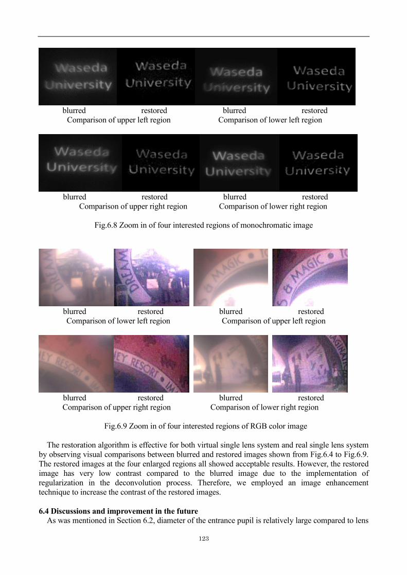
123

blurred restored blurred restored

Comparison of upper left region Comparison of lower left region


Comparison of upper right region Comparison of lower right region

Fig.6.8 Zoom in of four interested regions of monochromatic image


Comparison of lower left region Comparison of upper left region


Comparison of upper right region Comparison of lower right region

Fig.6.9 Zoom in of four interested regions of RGB color image

The restoration algorithm is effective for both virtual single lens system and real single lens system

by observing visual comparisons between blurred and restored images shown from Fig.6.4 to Fig.6.9.

The restored images at the four enlarged regions all showed acceptable results. However, the restored

image has very low contrast compared to the blurred image due to the implementation of

regularization in the deconvolution process. Therefore, we employed an image enhancement

technique to increase the contrast of the restored images.

6.4 Discussions and improvement in the future As was mentioned in Section 6.2, diameter of the entrance pupil is relatively large compared to lens


124

diameter, which results in augmented spherical aberration. As a result, parallel light beams coming

from different distance to the optical axis converge to different positions on the image side, which

explains blurring around center of the blurred image in Fig.6.5 and Fig.6.7. This problem can be

solved by decreasing diameter of the entrance pupil but it will reduce light irradiation on the image

sensor simultaneously. Therefore, one has to scarify the image brightness and contrast to obtain a

spherical aberration-free image. Fortunately, image enhancement could also be used in this case. In

addition, we applied PSF at the design wavelength (587.6nm) to RGB image for simplicity. More

precise restored image can be expected if PSFs at different wavelengths are applied to different color

planes, e.g. PSFs in the range 401nm~500nm are applied to B-plane, 501nm~600nm to G-plane and

601nm ~700nm to R-plane. Moreover, we took photo on a printed paper using the real single lens

camera in this experiment. In future work, experiment on a 3-dimensional spatial object that is located

at a certain distance from the camera module is desirable. The spatial object can be considered a 2D

object as long as it is located in a plane perpendicular to the optical axis of the camera. Finally, as to

the future development of the single lens imaging system, we considered four aspects: 1) Further

slimness is necessary and achievable by employing plano-convex single lens with higher refractive

index such as LaSF9 (refractive index is 1.850) and smaller central thickness. We are currently

developing a real cell phone camera system that could reduce the overall thickness to approximately

1.0mm. 2) Currently, the blur restoration algorithm is realized by computer program, implementation

of the algorithm on a real time image signal processor (ISP) in a camera is highly desirable. 3)

Incorporating other camera features such as autofocus and zooming features so as to compete with

other types of next-generation camera. 4) Although the overall thickness of the camera can be reduced

by employing single lens system, the overall dimension of cell phone or stand-alone camera is not

easy to be reduced due to the use of silicon semiconductor technology. A promising breakthrough of

semiconductor technology: Carbon nanotube (or CNT) that is in nanometer scale could probably

replace silicon and achieve further minimization of the future camera phones and stand-alone

cameras.

6.5 Conclusion

In this chapter, we introduced a real double convex spherical single lens system and successfully

restored the radially variant blur by employing an improved algorithm based on the polar coordinate

domain deconvolution method introduced in Chapter 5. Experiment on a 3Megapixels, 2D

monochromatic image and a RGB photograph suggests that the blur restoration algorithm is effective

on the real spherical single lens imaging system. Our next step is to fabricate a real single lens camera

module for cell phones using plano-convex surface and material with higher refractive index such as

LaSF9, which can reduce the overall thickness to approximately 1.0mm.

126

Chapter 7 Conclusions


127


This chapter summarizes this study on the following three aspects: 1) originality and objectives of

this research; 2) current achievements in this research; 3) future research plan for the single lens

system.

The originality of this research can be summarized as follows: this study provides a new option for

future cell phone camera because the number of lens elements is limited to one so that thickness of the

camera could be reduced to unprecedented level by using appropriate lens. The optical aberrations

caused by the single lens system can be minimized by digital image processing techniques, even if the

conventional optical means is not used. Therefore, there are two objectives in this study: 1) Replace

compound lens system with a spherical single lens system in order to reduce thickness of the cell

phone camera; 2) Correct optical aberrations of the single lens system by using digital image

processing.

In this dissertation, we demonstrated a virtual spherical single lens system designed by optics

design software CODEV and successfully corrected distortion, lateral chromatic aberration and

restored the radially variant blurred image for the resulting images produced by this virtual system. In

addition, a real spherical single lens system was also developed to evaluate proposed algorithms and

satisfactory results were obtained by experiment. These all proved the possibility of a spherical single

lens system to replace the compound lens camera system.

However, this system needs further improvement such as 1) Implementation of the proposed

algorithms on a real time image signal processor (ISP) in a camera. 2) Incorporating autofocus and

zooming features etc. 3) Further slimness of both embedded camera and the cell phone body. With the

rapid development of optical, electrical, electronics and semiconductor technology, we believe that

these improvements will be realized continually in the not too distant future.

Acknowledgments

128

Acknowledgments

As the author of this Ph.D dissertation, I would particularly thank my supervisor, Prof. Toshitsugu

Ueda, a renowned professor in the field of MEMS, sensor and sensing technology, for his direction

and kind assistance in this project. It is Prof. Ueda’s insightful advices and comments that facilitate

the research on the single lens imaging system. Prof. Ueda has financially supported this project since

5 years ago and actively devoted himself to this project. Without his support and contribution, this

research cannot be continued.

We wish to express our sincere appreciation to Prof. Hiroshi Inujima and Prof. Sei-ichiro Kamata,

who are the Vice-examiners of this Ph.D dissertation. Prof. Inujima is a renowned professor and

specialist in the field of machine diagnosis and spectrum analysis. Prof. Kamata is also a well-known

specialist and famous for his achievements in the research discipline of image processing and pattern

recognition and applications. Their comments and advices on revising this dissertation are crucial to

the completion of the final version.

As a long term partner of this research since 2005, Mr. Ikumi Minema has positively participated in

this project, provided useful suggestions on improving the correction algorithms, shared his creative

ideas with us and most importantly, made great effort to facilitating realization of real time

implementation of our algorithms on a cell phone ISP. His endeavor is highly appreciated.

We are also indebted to Prof. Lev Zimin of Kyushu Institute of Technology, who helped us build

the real double convex spherical single lens module. His professional skill and experience on imaging

system ensured the successful fabrication of the real lens system.

We want to express our thankfulness to Prof. Joanna Pawlat, who has been carefully reviewed and

revised the dissertation.

We also would like to take this opportunity to express our gratefulness to Mr. Tsuno, a technical

supporter in Ueda Laboratory, who provided powerful hardware environment for smoothly running

our aberration correction algorithms.

Mr. Tomita, who is an employee in GE Corp. , has been kindly helping us revise this Ph.D

dissertation. We also feel grateful to him.

Moreover, we want to thank all members of Ueda Lab., especially Dr. Satoshi, Ikezawa, who

provided useful information and suggestions throughout the creation of this Ph.D dissertation.

Finally, I am grateful to my parents who gave me a desire for knowledge and courage to walk

through all sorts of difficulties in my life.

Yupeng Zhang

Feb.6, 2011

Achievements

129

Achievements

• 学術誌原著論文 (Journal Papers)

• 1. Yupeng Zhang, Toshitsugu Ueda , “Deblur of radially variant blurred image for single lens

system”, IEEJ Trans. Electrical and Electronic Engineering. Vol.6 S1 (Feb.,2011) (in press)

• 2. Yupeng Zhang, Toshitsugu Ueda , “Design of a singlet lens and the corresponding aberration

correction approaches for cell phone camera”, IEEJ Trans. Electrical and Electronic Engineering.

Vol.5 No.4 (Jul.,2010), pp.474-485

• 3.Yupeng Zhang, Toshitsugu Ueda, “Field-dependent distortion coefficient and backward

mapping for distortion correction of singlet lens cameras”, IEEJ Trans. Electrical and Electronic

Engineering.Vol.5 No.2 (Mar.,2010), pp.203-210

• 4.Yupeng Zhang, Ikumi Minema, Toshitsugu Ueda,“A texture dependent interpolation for barrel

distorted and longitudinal chromatic aberrated image”, IEEJ Trans. Sensors and Micromachines, Vol.128, No.11 (Nov.,2008),pp.423-430

• 査読のある国際会議、シンポジウム論文(International Conference Papers with Review)

5. Yupeng Zhang, Ikumi Minema, Lev Zimin and Toshitsugu Ueda. “A Real Double-convex

Spherical Single Lens System with Blur Restoration Feature”, The 2011 International

Conference on Communication and Electronics Information (ICCEI 2011), Haikou, China (Feb.

22-24, 2011) (Accepted)

6. Yupeng Zhang, Ikumi Minema, Toshitsugu Ueda,"Restoration of Radially Blurred Image

Created by Spherical Single Lens System of Cellular Phone Camera", IEEE Sensors 2010

Conference,Hawaii, pp.1333-1337, USA, (Nov. 1-4, 2010)

7.Yupeng Zhang, Ikumi Minema, Toshitsugu Ueda. “Geometrically distorted image correction for

single lens using decimal number mapping. ” Proceedings of the 10th IASTED International

Conference on Signal and Image Processing (SIP2008),pp.26-31,Hawaii, USA (Aug.,2008)

8.Yupeng Zhang, Ikumi Minema, Toshitsugu Ueda , “Case analysis oriented interpolation and a

two-step interpolation after correction of barrel distortion and lateral chromatic aberration,”

Proceedings of the 24th Sensor Symposium, pp. 236-239,Tokyo,Japan (Oct.,2007)

• 国内会議発表 (Domestic Conference Presentation)

• 9. Yupeng Zhang, Ikumi Minema, Toshitsugu Ueda, “Blur restoration for a spherical single lens

system of cell phone camera”, 4th IPS International Collaboration Symposium,pp.57, Fukuoka,

Japan (Nov. 17-19, 2010)

• 10. Yupeng Zhang, Ikumi Minema, Toshitsugu Ueda ,“Correction of barrel distortion for simple

digital camera systems,” Joint Conference of Electrical and Electronics Engineers in Kyushu, pp.

470 (Sep. 2006)

受賞等 (Award)

・ Finalist for IEEE Sensors 2010 Conference Best Student Paper Award

correction of spherical single lens aberration using digital ...

Documents

Transcript of correction of spherical single lens aberration using digital ...