arX

iv:a

stro

-ph/

0604

301v

1 1

3 A

pr 2

006

Astronomy & Astrophysicsmanuscript no. 5180reza c© ESO 2014January 20, 2014

The flow field in the sunspot canopy

R. Rezaei1, R. Schlichenmaier1, C.A.R. Beck1, and L.R. Bellot Rubio1,2

1 Kiepenheuer-Institut fur Sonnenphysik, Schoneckstr. 6, 79104 Freiburg, Germany2 Instituto de Astrofisica de Andalucia (CSIC), Apdo. 3004, 18080 Granada, Spain

Received 10 March 2006/Accepted 28 March 2006

ABSTRACT

Aims. We investigate the flow field in the sunspot canopy using simultaneous Stokes vector spectropolarimetry of three sunspots (θ= 27◦, 50◦,75◦) and their surroundings in visible (630.15 and 630.25 nm) and near infrared (1564.8 and 1565.2 nm) neutral iron lines.Methods. To calibrate the Doppler shifts, we compare an absolute velocity calibration using the telluric O2–line at 630.20 nm and a relativevelocity calibration using the Doppler shift of StokesV profiles in the umbra under the assumption that the umbra is atrest. Both methods yieldthe same result within the calibration uncertainties (∼ 150 m s−1). We study the radial dependence of StokesV profiles in the directions of diskcenter and limb side.Results. Maps of StokesV profile shifts, polarity, amplitude asymmetry, field strength and magnetic field azimuth provide strong evidence forthe presence of a magnetic canopy and for the existence of a radial outflow in the canopy.Conclusions. Our findings indicate that the Evershed flow does not cease abruptly at the white–light spot boundary, but that at least a part ofthe penumbral Evershed flow continues into the magnetic canopy.

Key words. Sun: photosphere – Sun: sunspots – Sun: magnetic fields

1. Introduction

From the pioneering work of Evershed (1909), we know thatthere is a flow field in the sunspot penumbra, which leads toa line shift and line asymmetry. For sunspots outside the diskcenter, it manifests in blue shifted spectral lines in the centerside and red shifted spectral lines in the limb side. The penum-bral fine structure has a close relation with the Evershed flow. Itis generally accepted that the flow channels are more horizontalthan the background field (Solanki 2003). Because spectropo-larimetric data has lower spatial resolution than narrow bandmagnetograms, many questions regarding both the Evershedflow and the fine structure of the penumbra have remained (e.g.Solanki 2003; Bellot Rubio 2004). There are also controversialarguments about the continuation of the Evershed flow outsidethe sunspot.

Brekke & Maltby (1963) studied horizontal variations ofthe Evershed flow. Investigating 2500 sunspot spectra, theyre-ported that at the outer penumbral boundary “the velocity fallsabruptly to zero”. Wiehr et al. (1986) observed a sharp de-crease of the Evershed effect and magnetic field at the visibleboundary of sunspots. Using only StokesI spectra, they arguedthat line–core shifts and line asymmetries are “strongly” lim-ited to the continuum boundary of sunspots. Wiehr & Balthasar(1989), Schroter et al. (1989) and Title et al. (1993) confirmedthe result of Brekke & Maltby (1963). Wiehr (1996) renewedhis argument that the StokesI profile asymmetries of Ni I

543.6nm (g= 0.5) and Fe I 543.5nm (g= 0) “disappear” withinless than one arcsec from the penumbral border. Hirzberger &Kneer (2001) observed two sunspots at heliocentric angles of31◦and 20◦; they reported a sharp decrease of the Evershed flow(intensity profile asymmetry) at the penumbral boundary, usingStokesI of the non–magnetic Fe I 557.6nm and Fe I 709.0nmlines.

In contrast, Sheeley (1972) stated that there is a horizon-tal flow in the plage–free photosphere surrounding sunspotswith an average velocity of∼0.5 – 1 km s−1. Kuveler & Wiehr(1985) did not find a sharp change in the Evershed flow atthe penumbral boundary. Dialetis et al. (1985), Alissandrakiset al. (1988), and Borner & Kneer (1992) confirmed this re-sult. Giovanelli & Jones (1982) reported magnetogram obser-vations of diffuse, almost horizontal magnetic field surround-ing two spots at moderate heliocentric angles. Taking StokesV and I profiles of the 1.56µm iron lines for two limb spots,Solanki, Montavon, & Livingston (1994) found that the mag-netic field of sunspots continues beyond the visible bound-ary and forms an extensive canopy above a non–magneticlayer. These authors computed the canopy base height and re-ported that around 10 % of the Evershed flow continues intothe magnetic canopy. Rimmele (1995a, b) also found no sharpboundary in time–averaged velocity maps of a sunspot closeto the disk center. After observing the Fe I 557.6 nm line witha narrow–band filtergraph, he obtained different velocities atdifferent bisector levels which do not decrease abruptly at the

2 Rezaei et al.: The flow field at the sunspot canopy

sunspot boundary. Solanki et al. (1999) repeated their claimsabout continuation of the Evershed flow by consideringV andIsignals of the 1.56µm iron lines for another sunspot close to thelimb (µ = cosθ=0.22). Computing the amplitude of the az-imuthal velocity variation, Schlichenmaier & Schmidt (2000)did not find a drop of the line–core velocity of Fe II 542.5 nmat the penumbral boundary. Therefore, this long standing dis-agreement about continuation/termination of the flow field atthe sunspot boundary was intensified.

However, it is important to note that none of the men-tioned authors observed the full Stokes parameters of the tar-get spots. Moreover, a majority of them only used StokesIprofiles, which suffer from stray light contamination. Here,we present simultaneous spatially co–aligned full Stokes spec-tropolarimetric observations of three sunspots and their sur-roundings in visible (630.15 and 630.25nm) and near infrared(1564.8 and 1565.2 nm) neutral iron lines. These co–temporaland co–spatial observations of the full Stokes vector providevaluable information not only about magnetic field strengthinthe canopy, but also about the field orientation as emphasizedby Solanki et al. (1994). The near–IR neutral iron lines mostlyform deep in the atmosphere, while the contribution function ofthe visible iron lines at 630 nm peaks in higher layers (CabreraSolana et al. 2005). As these lines form in different atmosphericlayers and have large Zeeman sensitivities, they provide a pow-erful tool to study the properties of the canopy, its flow fieldand vertical structure.

Considering the fact that the Stokes profiles ofQ, U, andV are formed only in a magnetized atmosphere, this data setcontains information regarding the extension of the magneticcanopy and the Evershed flow outside the white–light sunspotboundary. In sections 2 and 3, we explain our observations anddata reduction in detail. In section 4, the spatial variation ofthe flow field is investigated using two independent methods.Conclusions and comparisons are discussed in Sect. 5.

2. Observations

Three isolated sunspots (cf. Fig. 1) were observed at theGerman Vacuum Tower Telescope (VTT) in Tenerife, August2003. Simultaneous co–aligned spectropolarimetric data withthe Tenerife Infrared Polarimeter (TIP) and the POlarimetricLIttrow Spectrograph (POLIS) were recorded. The TIP(Collados 1999; Martinez Pillet et al. 1999) observed fullStokes profiles of the infrared iron lines at 1564.8nm (g= 3)and 1565.2nm (g= 1.53). The visible neutral iron lines at630.15 nm, 630.25nm, and Ti 630.38nm were observed withthe POLIS (Schmidt et al. 2003; Beck et al. 2005a).

For the spots 1 and 3, the scanning step–size was 0.35 arc-sec, while for spot 2 it was 0.4 arcsec. Spatial sampling ofthe TIP maps along the slit was 0.35 arcsec. For the POLIS,the spatial sampling along the slit was 0.15 arcsec (Beck etal. 2005a). To improve the signal–to–noise ratio and to haveacomparable spatial resolution as in the infrared data, we bin thedata along the slit by a factor of 3. The pixel size of these newmaps along the slit is 0.44 arcsec. The spectral sampling of 2.97pm for TIP and 1.49 pm for POLIS leads to a velocity disper-sion of 570 m s−1 and 700 m s−1 per pixel, respectively. Seeing

Table 1. Properties of the observed sunspots.θ is the heliocen-tric angle. The last column is the scanning step–size in arcsec.

Spot No. Date Active Region θ (◦) step–size1 09/08/2003 10430 27 0.352 03/08/2003 10425 50 0.403 08/08/2003 10421 75 0.35

conditions during the observations were good and stable. Weused the Correlation Tracker System (Schmidt & Kentischer1995; Ballesteros et al. 1996) to compensate for image motion.We estimate the spatial resolution to be about 1.0 arcsec forthespots 1 and 2 and 1.5 arcsec for the spot 3. The duration of theobservations for each sunspot was around 10 minutes.

The spectropolarimetric data of both TIP and POLIS havebeen corrected for instrumental effects and telescope polariza-tion with the procedures described in Collados (1999; MartinezPillet et al. 1999) for the TIP and Beck et al.(2005a, b) for thePOLIS. Remaining cross–talk in our data sets is of the orderof 10−3 Ic. Table 1 summarizes the characteristics of the threeobservations. The spot closest to the limb was atθ= 75 deg.

3. Data analysis

In this section, we explain the data reduction and present ourdefinition for the sunspot boundary. Then we investigate twoindependent methods of velocity calibration. Finally, we ex-tract vector magnetic field parameters.

3.1. Pre-processing

We use a continuum intensity threshold to define umbral datapoints and their mean position, the umbral center. After that,we draw a radial line from the umbral center in azimuthal di-rections (in 0.5◦ steps). The point at which this line crossesthe penumbral white–light boundary defines the sunspot borderand radius in this direction. The continuum threshold whichareused at the penumbral border are 0.8 and 0.9Ic for the visibleand infrared data respectively. These crossing points define aclosed path (contour) around each sunspot (cf. Fig. 1, left col-umn).

All polarization signals,Q(λ), U(λ), V(λ), and the total lin-ear polarization profiles,L(λ)=

√

Q(λ)2 + U(λ)2, are normal-ized by the local continuum intensity,Ic, for each pixel, i.e.,V(λ)≡V(λ)/Ic. The rms noise level of Stokes parameters inthe continuum isσ= 3 – 5×10−4 Ic for the infrared lines andσ= 1.5×10−3 Ic for the visible lines. Only pixels withV sig-nals greater than 5σ for TIP (3σ for POLIS) are included inthe analysis. Positions and amplitudes of the profile extrema inall Stokes parameters are obtained by fitting a parabola to eachlobe.

For the POLIS data, we apply a correction along the slit be-fore calibrating the velocity. In this direction, there is acurva-ture in the profiles due to the small focal length of the spectro-graph. For each scan step, a third order polynomial is fitted topositions of the 630.20nm telluric line–cores along the slit. Allprofiles in that scan step are shifted with the resulting curve.

Rezaei et al.: The flow field at the sunspot canopy 3

Fig. 1. From left to right:continuum intensity maps of the sunspots, integrated circular polarization (∫

|V(λ)|dλ), the integratedlinear polarization signal (Lt =

∫

L(λ)dλ), and polarity in Fe I 1564.8nm line.From top to bottom:spot 1, spot 2, and spot 3.Axis labels are spatial dimensions in arcsec. The numbers onthe upper–right corners are the heliocentric angles of the spots.In the white–light maps, the left arrows show the disk centerdirections. Note that the magnetic field clearly extends over thewhite–light boundary along the line connecting sunspot to the disk center in theV maps and perpendicular to this line inLt maps.

This correction amounts at most to∼ 4 (spectral) pixels shiftbetween upper most and lower most spatial pixels. Final mapsof the line–core velocity of the telluric line are quite uniformwith a small dispersion (standard deviation) in the umbral re-gion, e.g. around 0.11 pixel (≡ 77 m s−1) for the spot 1. Usingthis telluric rest–frame, we calibrate StokesV andI shifts.

3.2. Velocity calibration

We consider two different calibration methods. The firstmethod is based on StokesV profiles of the umbra. Assumingthat the umbra is at rest, we select quite antisymmetric StokesV profiles. The StokesV profile is expected to be strictly an-tisymmetric with respect to its zero–crossing wavelength,ifno velocity gradients with height is present and if LTE ap-plies (Auer & Heasley 1978; Landi Degl’Innocenti & Landolfi1983). Hence, the mean position of these profiles is assumedto define arest–frame. To confirm the assumption of the umbraat rest, we perform an absolute velocity calibration using thetelluric lines in the POLIS data. At the end of this section, we

compare the two calibration methods. Results are completelyconsistent and differences are less than the calibration error.

3.2.1. Velocity calibration using Stokes V profiles ofthe umbra

We attribute a relative amplitude asymmetry,δa, to eachV(λ)profile. It is defined as the asymmetry between the amplitudesof the two lobes of StokesV by:

δa =ab − ar

ab + ar,

whereab andar are the absolute amplitudes of blue and redlobes, respectively. The center of eachV(λ) profile is defined asthe midway between its maximum and minimum. This quantityis better than deriving the zero–crossing by a linear regression,because it is less affected by magneto–optical effects. First,all umbral profiles with an amplitude asymmetry lower than athreshold are selected, which defines a class correspondingto arow in Table 2. Then, the relative velocity of each selected pro-file with respect to the mean value of the class (reference point)

4 Rezaei et al.: The flow field at the sunspot canopy

Table 2. From top to bottom:spot 1, 2, and 3. The first col-umn is the maximum amplitude asymmetry in each class.d1

(d2) shows the velocity dispersion of the selected umbral pro-files in infrared (visible) lines in each row. % IR (vis) givesthenumber of umbral profiles in percent of all umbral pixels withδa less than the threshold. The fourth and the last columns aredifference of velocity reference point of each class relative tothe final result (|δa| ≤ 0.05). The last row gives number of totalumbral profiles. Velocities are in m s−1.

max. |δa| d1 % IR ref: IR d2 % vis ref: vis0.10 143 100 -6 112 100 00.07 143 98 -6 112 99 00.05 137 96 – 112 98 –0.03 143 66 12 112 91 00.02 137 41 18 112 74 00.01 125 20 41 119 42 00.10 108 99 0 155 77 140.07 108 96 6 148 61 70.05 108 71 – 155 50 –0.03 114 40 6 183 28 -70.02 114 25 12 211 17 -140.01 120 11 41 – – –0.10 205 79 18 268 91 140.07 216 65 12 268 83 00.05 176 52 – 282 75 –0.03 170 41 -24 275 59 -350.02 114 31 -41 268 42 -350.01 80 16 -59 247 23 -28

Ntot 1 /2 / 3 649/ 321/ 153 434/ 263/ 135

is determined. So each class has a velocity dispersion aroundits mean value which is defined to be zero. The velocity dis-persions for different classes are similar (d1 andd2 in Table 2).These are the main uncertainties in the StokesV velocity cal-ibration. The difference between reference point of each classand the|δa| ≤ 0.05 class is given in Table 2 (fourth and lastcolumns). We select the mean position of a set of quite anti-symmetric umbral profiles with|δa| ≤ 0.05 as the sunspot rest–frame, which is a compromise between low amplitude asym-metry and good statistics (Table 2).

In spot 3, the magnetic neutral line lies inside the um-bra, because the spot is close to the limb. Therefore, insidethe sunspot the longitudinal component of the magnetic fieldalong the line of sight is weaker than the transverse component.Hence, the StokesV profiles are not reliable for the calibrationpurpose. For this reason, we use the linear polarization compo-nents instead. We decided to use the profile center of the StokesQ (position of theπ component) in this case and use the am-plitude asymmetry of theσ components inQ as a measure ofthe line antisymmetry. The dispersion of the velocity referencepoints in the selected umbral pixels (spot 3) is slightly higherthan for spots 1 and 2 (Table 2). We estimate a maximum cali-bration error for the spot 3 of∼250 m s−1. This does not affectour conclusions, because velocity values in spot 3 are largerthan in spots 1 and 2. From the velocity dispersions in eachclass (d1 andd2), we estimate that we achieve a precision of

Table 3. Wavelengths of the spectral lines in the POLIS data.The laboratory wavelengths are from Higgs (1960, 1962). Therest value includes the gravitational redshift (∆λ = 2.12 ×10−6λ).

Laboratory (Å) rest (Å) air (Å)Fe I 6301.4990 6301.5124 -O2 - - 6302.0005Fe I 6302.4920 6302.5054 -O2 - - 6302.7629Ti I 6303.750 6303.763 -

±150 m s−1 for the spots 1 and 2 and±250 m s−1 for the spot3 in the TIP and POLIS data, respectively1.

3.2.2. Absolute velocity calibration

Using the telluric lines in the POLIS data, it is possibleto perform an absolute velocity calibration for these datasets (Schmidt & Balthasar 1994; Martinez Pillet et al. 1997;Sigwarth et al. 1999). We use the 630.20nm line, because it isless influenced by the solar iron lines in the umbra than the O2–line at 630.27nm. We only correct line–core positions for thecurvature of the spectrograph as explained in Sect. 3.1. Then,the radial velocity between the observatory and the sunspotisdetermined. We use the values of Balthasar et al. (1986) for thesunspot angular rotation ([14.551,-2.87], cf. their Eq. (1)) tocompute the radial velocity components: the earth rotation, theearth orbital motion and the solar rotation. Total radial veloci-ties for the spots 1, 2, and 3 (sum of the three components) are0.253, 0.862 and 1.327 km s−1, respectively. These values takeinto account the line of sight component of the solar rotation,which amounts to 0.918, 1.438, and 1.971 km s−1. Gravitationalcorrection is also considered for all solar lines (Table 3).Here,the rest–frame for each resolution element is the position of thetelluric line plus a constant shift which includes proper correc-tion for the radial velocity. In other words, there is a referencepoint in each resolution element different from the others.

Source of errors Apart from the precision of the solar centerand sunspot positions, the main challenge is to determine theexact sunspot angular rotation. Angular rotation of sunspotsdepends on the age and probably the phase of the solar cy-cle. It is also affected by the sunspot proper motion. So, theradial velocity values remain uncertain within∼±100 m s−1.Moreover, there are some errors in positioning during the ob-servations. For example, 5 arcsec error in the solar longitudecreates an error of∼ 15 m s−1 in the radial velocity (dependingon the position). Pixel by pixel variation due to different timeand slit positions cause a maximum error of∼ 10 m s−1 betweenthe first and the last scan steps. Therefore, we conclude thatforthe absolute velocity calibration the precision is±150 m s−1.

Oscillations in the photospheric level of the umbra may in-duce errors in the StokesV calibration. However observationsimply that such fluctuations are small. Martinez Pillet et al.

1 Our convention is that positive values correspond to redshift.

Rezaei et al.: The flow field at the sunspot canopy 5

Table 4. Mean values and dispersions of the umbral veloci-ties for the 630.25nm iron line in km s−1. The last columnshows uncertainties in the StokesV and absolute calibrationsfor the spots 1 and 2. These values for the spot 3 are 0.211 and0.282 km s−1 respectively. It confirms our principal assumptionthat the umbra is at rest (within our calibration error).

spot 1 StokesI StokesV errorStokesV calib 0.085± 0.242 -0.023± 0.059 0.112absolute calib -0.135± 0.258 -0.258± 0.060 0.176

spot 2StokesV calib -0.158± 0.143 -0.038± 0.088 0.176absolute calib -0.168± 0.135 -0.044± 0.072 0.211

(1997), for example, studied a large sample of active regionsand reported an umbral velocity of 65 m s−1 due to umbral os-cillations. Balthasar & Schmidt (1994) also investigated fiveminute oscillations in the umbra and reported an amplitude of90 m s−1 (rms).

3.2.3. Comparison of the two calibration methods

In order to check the assumption that the umbra is at rest, wecompare the two calibration methods. Subtracting the corre-sponding velocity maps for Fe I 630.25 nm yields a differencemap that show low amplitude variations, definitely less thanthecalibration uncertainties. It is important to note that we useda constant velocity reference point in the first method for thewhole image, while in the absolute calibration we used differ-ent reference points (one for each spatial pixel). To compare theabsolute calibration with the first method, we define a mean ref-erence point for the absolute calibration, the corrected telluricline position in the umbra.

Comparing StokesV and absolute calibrations, there aresmall differences between them and also small dispersions ineach one: Table 4 lists the mean umbral velocities for thewholeumbrafor the Fe I 630.25nm line obtained from both methods.The average StokesV umbral velocities with absolute calibra-tion confirm that our basic assumption, taking the umbra at rest,is correct. Average line–core velocities are also less thanourcalibration errors. Their tendency for a blueshift is probablydue to stray light contamination from the quiet sun. However,in the StokesV absolute calibration there is a tendency for ablueshift because the average velocities of the whole umbrain-clude umbral dots and periphery points. These lead to the weakblueshifts in the umbra, comparable to our calibration preci-sion. There are reports of strong upflows in the umbra of pre-ceding spots in bipolar pairs (e.g. Sigwarth 2000); howeverallthree spots were isolated. Our results do not exclude that thereare some oscillations in the umbra, but the amplitudes shouldbe less than our precision limit of± 150 m s−1 (as reported by,e.g. Lites et al. 1998; Bellot Rubio et al. 2000a).

The absolute calibration confirms our first method basedon the StokesV profiles of the umbra. Therefore, we can con-fidently use this method where an absolute calibration is notpossible like for the TIP data.

3.3. Magnetic field parameters

To investigate the flow field in the canopy, we calculate line pa-rameters for allregular V(λ) profiles, i.e. profiles which showtwo clear lobes. The quantities derived are positions and am-plitudes of the peaks, area and amplitude asymmetries, andthe magnetic field strength. We also analyzeQ(λ), U(λ), andL(λ) of the TIP data in order to have a measure for the inclina-tion and azimuth of the magnetic field. We construct maps offield strength, azimuth, amplitude asymmetry of StokesV, andStokesV velocities (Fig. 2). Comparing the second and thirdcolumns of Fig. 2, it is clear that the magnetic neutral line inthe visible is shifted outward with respect to the infrared line.The field strength is calculated using the StokesV splitting ofthe 1564.8nm line. The line is a Zeeman triplet which is in thestrong field limit for B > 0.03 T; so we can use the distancebetween theσ component and the profile center as a measureof the magnetic field strength (e.g. Stix 2002) by:

∆λ = 4.67× 10−18λ2geffB

wheregeff is the effective Lande factor,∆λ andλ are in nm,and B is in tesla. This is not an exact method, especially forweak fields. So these estimates are upper limits for the weakmagnetic field of the canopy. This method fails along the mag-netic neutral line. Maps on the left column of Fig. 2 show thefield strength.

Considering the fact that these Stokes profiles are formedin the weak field limit in the canopy, one may use the ratioof theσ components of the linear and circular polarization toapproximate the magnetic field inclination and azimuth (e.g.Stix 2002; Solanki 1993)

V√

Q2 + U2∼

cosγ

sin2 γand

UQ∼ tan(2χ)

whereγ is the inclination with respect to the line of sight andχ is the azimuth with respect to the celestial N–S direction. Inthe weak field limit, these ratios are independent of the fieldstrength. Computing field orientation in this way is not as ac-curate as an inversion. However, it is sufficient for our purposeto check whether or not the field geometry in the canopy fol-lows the same pattern as in the spot. The azimuth maps in Fig.2 (right column) show the same pattern inside and outside thespot in the canopy. Thus, the canopy can be distinguished inthese maps from the separate magnetic elements, which showdifferent azimuth and field strength.

Because linear polarization signals are usually weaker thanthe circular polarization, it is not possible to compute thefieldazimuth for all pixels with a reasonableV signal. Moreover,the field strength in the canopy is much smaller than in thespot. For this reason, we have smaller coverage in the azimuthmaps, which come from linear polarization signals, with re-spect to other maps which are based onV signals (Fig. 2).Pattern of various parameters outside the spot in Fig. 2 showasmooth change at the spot boundary. In other words, the mag-netic field strength and orientation, and the flow field do notchangeabruptlyat the sunspot white–light boundary.

6 Rezaei et al.: The flow field at the sunspot canopy

Fig. 2. From left to right: field strength,B, in Gauss (10−4 T); StokesV velocity in 1564.8nm in km s−1; StokesV velocity in630.25 nm in km s−1; StokesV amplitude asymmetry in 630.25nm (%); magnetic field azimuthin degree.From top to bottom:spot 1, spot 2, and spot 3. As it is clear in the StokesV amplitude asymmetry of spot 3, there are significant amplitude asymmetriesin the umbra due to the presence of the magnetic neutral line.Also note the usually larger velocities outside the penumbralboundary in the visible (630.25nm) than infrared (1564.8nm) line. Magnetic field strength and azimuth obviously indicate thatthe magnetic field of sunspots continue outside the white–light boundary with the same orientation. Separate magnetic elementsmay be easily distinguished in these maps.

4. Radial outflow in the canopy

In this section, we define the magnetic canopy to be distin-guished from the isolated magnetic elements. We investigateStokesV profiles in radial cuts, both on the limb and centersides. Box–car averaging in radial directions is another methodto investigate the canopy. Finally, we study the canopy exten-sion in our sunspots.

4.1. Canopy definition and isolated magnetic elements

The maximum distance at which there is a magnetic field alongwith a flow (with consistentsign and gradient) varies for dif-ferent spots. We attribute a pixel in a radial cut to the sunspotcanopy, if it demonstrates all the properties below:

1. It has the same magnetic polarity and velocity sign as thepreceding pixel closer to the spot boundary.

2. It shows the same inclination and azimuth patterns as thepreceding pixel closer to the spot boundary.

3. Both the absolute values of the velocity and magnetic fieldstrength decrease with respect to the preceding pixel or re-main constant.

The right column of Fig. 1 illustrates the polarity maps. It isclear that close to each spot, there is a unipolar–connectedre-gion that we attribute to the canopy. But as we go outward,some isolated magnetic elements appear with either differentpolarities or velocity signs. Therefore, thesign and gradientofvelocity at some of these points do not show a monotonic be-havior. These isolated magnetic elements are seen in various

Rezaei et al.: The flow field at the sunspot canopy 7

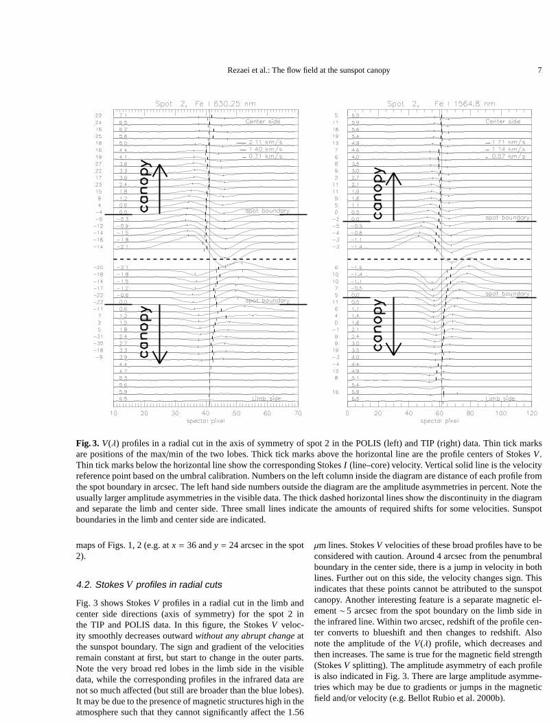
Fig. 3. V(λ) profiles in a radial cut in the axis of symmetry of spot 2 in thePOLIS (left) and TIP (right) data. Thin tick marksare positions of the max/min of the two lobes. Thick tick marks above the horizontal line are the profile centers of StokesV.Thin tick marks below the horizontal line show the corresponding StokesI (line–core) velocity. Vertical solid line is the velocityreference point based on the umbral calibration. Numbers onthe left column inside the diagram are distance of each profile fromthe spot boundary in arcsec. The left hand side numbers outside the diagram are the amplitude asymmetries in percent. Note theusually larger amplitude asymmetries in the visible data. The thick dashed horizontal lines show the discontinuity in the diagramand separate the limb and center side. Three small lines indicate the amounts of required shifts for some velocities. Sunspotboundaries in the limb and center side are indicated.

maps of Figs. 1, 2 (e.g. atx = 36 andy = 24 arcsec in the spot2).

4.2. Stokes V profiles in radial cuts

Fig. 3 shows StokesV profiles in a radial cut in the limb andcenter side directions (axis of symmetry) for the spot 2 inthe TIP and POLIS data. In this figure, the StokesV veloc-ity smoothly decreases outwardwithout any abrupt changeatthe sunspot boundary. The sign and gradient of the velocitiesremain constant at first, but start to change in the outer parts.Note the very broad red lobes in the limb side in the visibledata, while the corresponding profiles in the infrared data arenot so much affected (but still are broader than the blue lobes).It may be due to the presence of magnetic structures high in theatmosphere such that they cannot significantly affect the 1.56

µm lines. StokesV velocities of these broad profiles have to beconsidered with caution. Around 4 arcsec from the penumbralboundary in the center side, there is a jump in velocity in bothlines. Further out on this side, the velocity changes sign. Thisindicates that these points cannot be attributed to the sunspotcanopy. Another interesting feature is a separate magneticel-ement∼5 arcsec from the spot boundary on the limb side inthe infrared line. Within two arcsec, redshift of the profilecen-ter converts to blueshift and then changes to redshift. Alsonote the amplitude of theV(λ) profile, which decreases andthen increases. The same is true for the magnetic field strength(StokesV splitting). The amplitude asymmetry of each profileis also indicated in Fig. 3. There are large amplitude asymme-tries which may be due to gradients or jumps in the magneticfield and/or velocity (e.g. Bellot Rubio et al. 2000b).

8 Rezaei et al.: The flow field at the sunspot canopy

Fig. 4. The solid line is the line–core velocity and the dashedline is the StokesV velocity of Fe I 1564.8 nm in the limb sideof the spot 2. The vertical line is the penumbral boundary (±0.2arcsec for differences in neighbor pixels). Inside the spot,V andI Stokes velocities follow each other, while they show differentbehaviors outside the spot. Upper x-axis is the distance fromthe penumbral boundary in units of sunspot radius. The aver-aging box is 17×17 pixels to cover granules and intergranularlanes.

4.3. Box–car averages of the flow and fieldparameters in the sunspot symmetry axis

Comparison of the line–core and StokesV velocities plays animportant role in distinguishing the radial outflow in the canopyand the moat flow. We average velocities in small square boxesalong the symmetry axis of the sunspots. We have large cover-age outside the spot in the limb side of the spot 2; so we studythis case in detail. Inside the penumbra, the line–core velocitiesare smaller than the StokesV velocities, having a similar radialdependence (cf. Fig. 4). Outside the spot, the curves of line–core and StokesV velocities intersect each other. Thus, a fewarcsec outside the penumbral boundary, the value of the StokesV velocity in the visible/infrared is less than the correspond-ing StokesI velocity. The intersection points for the infraredlines are slightly closer to the sunspots than visible lines. Therange of the velocities in the canopy is∼ 0.5 – 2.0 km s−1. Highvelocity patches are rare. Roughly speaking, a velocity of 1.0km s−1 is common in the canopy of all the three spots. This isfar from the average values for the line–core velocities. Theseare around 0.6 – 0.7 km s−1 close to the sunspots, reaching∼ –0.2 km s−1 (the typical values for the convective blueshift) at theboundary of the moat cell. At these distances, there is no uni-formly connected canopy as described above. Magnetic fieldsof these regions are governed by the plage activity and isolatedmagnetic elements floating in the sunspot moat.

The contribution function of the iron lines at 630 nm peaksin higher layers relative to the lines at 1.56µm. Visible linesform in larger geometrical extents than the infrared lines.Inaddition, StokesV profiles form exclusively in the magneticpart of the atmosphere. The fact that we usually observe largerStokesV velocities in the visible than in the infrared in the

Fig. 5. This plot shows the radial variation on StokesV veloci-ties on the limb side of the spot 2. The solid line is the visibleFe I 630.25nm StokesV velocity and the dashed line is thesame for the near IR Fe I 1564.8nm. The vertical line is thepenumbral boundary (±0.2 arcsec for differences in neighborpixels). Inside the sunspot, the TIP data show larger velocitieswhile outside the spot, the POLIS data show larger values. Theaveraging box is 5×5 pixels in this diagram.

Fig. 6. Same as Fig. 5 for the magnetic field strength in the TIPdata.

canopy (Figs. 2, 5) implies that there is a flow in the magneticpart of the atmosphere which affects the visible lines more thanthe infrared lines. Observations by Balthasar et al. (1996)ofthe moat flow in non–magnetic lines resulted in low amplitudesmooth velocity field (∼ 0.5 km s−1), similar to velocities wefind in the StokesI data. Beside this, the spatial extension of themoat flow is much more than what we observe in the StokesV maps. There are also significant amplitude asymmetries inthe sunspot canopy (Figs. 2, 3) which indicate that there aregradients or jumps in the velocity field. Therefore, the line–core velocity is comparable with the moat flow velocity in non–magnetic lines while the StokesV velocity is not a reasonableproxy for the moat flow. Hence, we attribute line–core velocityto the moat flow and StokesV velocity to the canopy outflow.

Rezaei et al.: The flow field at the sunspot canopy 9

We find average amplitude asymmetries in the canopy pro-files of ∼10 %. These values are less than the maximum am-plitude asymmetry, which peaks in the middle/outer penumbra(Schlichenmaier & Collados 2002). Amplitude asymmetries ofthe canopy in spot 2 are given in Fig. 3. The profile asymme-try is one of the typical properties of the Evershed flow, whichwe observe in the canopy radial outflow. It is different fromthe amplitude asymmetry in plage and network which changesfrom one pixel to the next one. We usually observe graduallychanging amplitude asymmetries in nearby pixels (Fig. 3).

The magnetic field strength decreases smoothly outside thespot (Fig. 6). There is no sharp change at the penumbral bound-ary or within 1 arcsec. The lobe separation in the StokesVprofiles of the canopy is a measure of the minimum magneticfield. The smallest StokesV splitting observed are∼ 0.03 T. Aswe go outward and leave the uniform–connected canopy withcoherent flow field, disturbances in the observedV(λ) profilesincrease. At some point, StokesV splitting increases while theamplitude decreases (Fig. 3, limb side, Fe I 1564.8 nm line, pro-file at 5.9 arcsec).

The average canopy extensions of 1.2, 1.35, and 1.6 (±

0.05) penumbral radii for the spots 1, 2, and 3 depend almostlinearly on the cosine of the heliocentric angle. We observesimilar canopy extensions in the visible and infrared lines. Allthe three sunspots were observed with the same setup and ex-posure time. It may be possible to trace larger canopies closeto the disk center with longer exposure times, and hence highersignal-to-noise ratios.

5. Conclusion

We investigate the flow and magnetic field in the immediatesurroundings of three sunspots using spectropolarimetricdataobserved simultaneously at the VTT in two spectral regionsaround Fe I 1564.8nm and around Fe I 630.2 nm, with TIP andPOLIS, respectively. The existence of a radial outflow in thesunspot canopy is a matter of strong debate. Here, we providestrong evidence for the existence of the canopy, and for theexistence of a radial outflow in the canopy by analyzing Stokesprofiles.

To this end it is essential to properly calibrate the veloc-ity. We use two different calibration methods. The first one isbased on the assumption that the most antisymmetric profilesin the umbra reflect locations at rest. The second is an abso-lute calibration which uses the telluric line in the vicinity ofFe I 630.2nm, taking into account the relative motions betweenthe telescope and the surface of the sun. Both methods are con-sistent, which implies that antisymmetricV profiles in the um-bra represent a rest–frame.

Evidence for the existence of a canopy surrounding all threesunspots at various heliocentric angles is presented:(1) The polarization signal extends outside the sunspot white–light boundary up to 1.2, 1.35, and 1.6 penumbral radii for spotsatµ= 0.89, 0.64, and 0.26 respectively.(2) We find that velocities and the estimated magnetic fieldstrength vary smoothly across the penumbral boundary. Thereis no abrupt change within one arcsec, which corresponds toour spatial resolution.

(3) The field azimuth and polarity in the canopy follow the spotpattern.(4) Velocities determined from Doppler shifts of StokesV showa radial outflow in the surroundings of sunspots. The same istrue for line–core velocities from Stokes I, but as argued inSect. 4.3, the latter is related to the moat flow.(5) Significant amplitude asymmetries of StokesV exist almosteverywhere in the surroundings of sunspots, indicating depthgradients or discontinuities in the flow velocity.

All our findings are consistent with a magnetic canopysurrounding sunspots, which exhibits a discontinuity (magne-topause) rising with radial distance from the spot. Moreover,our findings indicate that the radial outflow in the canopy is anextension of the penumbral Evershed flow. The decreasingV–velocity with radial distance from the spot is consistent with arising canopy base, i.e. with a magnetopause which rises out-wards from the spot. Line–core velocities of StokesI persistoutwards in the surroundings of sunspots and are therefore at-tributed to the moat flow. As one would expect, the canopy ex-tension increases with heliocentric angle, and even at a smallheliocentric angle of 27◦ the canopy extension is at least 3 arc-sec, much more than the spatial resolution. Therefore, we con-clude that at least a part of the penumbral Evershed flow con-tinues in a magnetic canopy that surrounds sunspots.

Acknowledgements.We wish to thank Wolfgang Schmidt, HubertusWohl, and Dirk Soltau for useful discussions. Daniel Cabrera Solana(IAA) kindly provided the routine for the radial velocity calculation.

References

Alissandrakis, C.E., Dialetis, D., Mein, P. et al., 1988, A&A 201, 339Ballesteros, E., Collados, M. & Bonet, J.A., 1996, A&AS 115,353Balthasar, H. & Schmidt, W., 1994, A&A 290, 649Balthasar, H., Vazquez, M. & Wohl, H., 1986, A&A 155, 87Balthasar, H., Schleicher, H., Bendlin, C. & Volkmer, R., 1996, A&A

315, 603Beck, C., Schmidt, W., Kentischer, T. & Elmore, D., 2005a, A&A 437,

1159Beck, C., Schlichenmaier, R., Bellot Rubio, L.R. & Kentischer, T.,

2005b, A&A, 443, 1047Bellot Rubio, L.R., 2004, Sunspots as seen in polarized light, Reviews

in Modern Astronomy, 17, Ed. R.E. Scielicke, WileyBellot Rubio, L.R., Collados, M., Ruiz Cobo, B. et al., 2000a, ApJ

534, 989Bellot Rubio, L.R., Ruiz Cobo, B. & Collados, M., 2000b, ApJ 535,

489Bellot Rubio, L.R., Balthasar, H., Collados, M. & Schlichenmaier, R.,

2003, A&A 403, L47Borner, P. & Kneer, F., 1992, A&A 255, 307Brekke, K. & Maltby, P., 1963, Ann. d’Astrophys. 26, 383Cabrera Solana, D., Bellot Rubio, L.R., & del Toro Iniesta, J.C., 2005,

A&A 439, 687Collados, M., 1999, in ASP Conf. Ser. 184, Thirds Advances inSolar

Physics Euroconference: Magnetic Field and Oscillation, 3Dialetis, D., Mein, P., & Alissandrakis, C.E., 1985, A&A 147, 93Evershed, J., 1909, MNRAS, 69, 454Giovanelli, R.G. & Jones, H.P., 1982, Solar Phys 79, 267Higgs, L.A., 1960, MNRAS, 121, 421Higgs, L.A., 1962, MNRAS, 124, 51Hirzberger, J. & Kneer, F., 2001 A&A 378, 1078

10 Rezaei et al.: The flow field at the sunspot canopy

Kuveler, G. & Wiehr, E., 1985, A&A 142, 205Landi Degl’Innocenti, E. & Landolfi, M., 1983, Solar Phys 87,221Leka, K.D., & Steiner, O., 2001, ApJ 552, 354Lites, B.W., Thomas, J.H., Bogdan, T.J. et al., 1998, ApJ 497, 464Martinez Pillet, V., Lites, W. & Skumanich, A., 1997, ApJ 474, 810Martinez Pillet, V., Collados, M., Sanchez Almeida, J. et al., 1999,

in ASP Conf. Ser. 183, High Resolution Solar Physics: Theory,Observation, and Techniques, 264

Rimmele, R.T., 1995a, ApJ 445, 511Rimmele, R.T., 1995b, A&A 298, 260Schlichenmaier, R. & Collados, M., 2002, A&A 381, 668Schlichenmaier, R. & Schmidt, W., 2000, A&A 358, 1122Schmidt, W. & Balthasar, H., 1994, A&A 283, 241Schmidt, W. & Kentischer, T., 1995, A&AS 113, 363Schmidt, W., Beck, C., Kentischer, T. et al., 2003, AN 324, 300Schroter, E.H., Kentischer, T., & Munzer, H., 1989, in High Spatial

Resolution Solar Observations, O. van der Luhe (Ed.), NationalSolar Obs., Sunspot, NM, p. 299

Sheeley N.R., Jr., 1972, Solar Phys 25, 98Sigwarth, M., 2000, Rev Mod Ast, 13, 45Sigwarth, M., Balasubramaniam, K.S., Knolker, M. & Schmidt, W.,

1999, A&A 349, 941Solanki, S.K., 1993, Space Sci Rev, 63, 1Solanki, S.K., 2003, A&AR 11, 153Solanki, S.K., Montavon, C.A.P., & Livingston, W., 1994, A&A 283,

221Solanki, S.K., Finsterle, W., Ruedi, I. & Livingston, W., 1999, A&A

347, L27Steiner, O., 2000, Solar Phys 196, 245Stix, M., 2002, The Sun: An Introduction, SpringerTitle, A.M., Frank, Z.A., Shine, R.A. et al., 1993, ApJ 403, 780Wiehr, E., 1996, A&A 309, L4Wiehr, E. & Balthasar, H., 1989, A&A 208, 303Wiehr, E., Stellmacher, G., Knolker, M. & Grosser, H., 1986, A&A

155, 402