Near-Field Flow Structure and Entrainment of a Round Jet at ...

http://www.diva-portal.org

This is the published version of a paper published in Computation.

Citation for the original published paper (version of record):

Kabanshi, A. (2020)Near-Field Flow Structure and Entrainment of a Round Jet at Low Exit Velocities:Implications on Microclimate VentilationComputation, 8(4): 100https://doi.org/10.3390/computation8040100

Access to the published version may require subscription.

N.B. When citing this work, cite the original published paper.

Permanent link to this version:http://urn.kb.se/resolve?urn=urn:nbn:se:hig:diva-34338

computation

Article

Near-Field Flow Structure and Entrainment of aRound Jet at Low Exit Velocities: Implications onMicroclimate Ventilation

Alan Kabanshi

Department of Building Engineering, Energy Systems and Sustainability Science, University of Gävle,80176 Gävle, Sweden; [email protected]

Received: 26 September 2020; Accepted: 20 November 2020; Published: 23 November 2020 ��

Abstract: This paper explores the flow structure, mean/turbulent statistical characteristics of thevector field and entrainment of round jets issued from a smooth contracting nozzle at low nozzle exitvelocities (1.39–6.44 m/s). The motivation of the study was to increase understand of the near field andget insights on how to control and reduce entrainment, particularly in applications that use jets withlow-medium momentum flow like microclimate ventilation systems. Additionally, the near field offree jets with low momentum flow is not extensively covered in literature. Particle image velocimetry(PIV), a whole field vector measurement method, was used for data acquisition of the flow from a0.025 m smooth contracting nozzle. The results show that at low nozzle exit velocities the jet flowwas unstable with oscillations and this increased entrainment, however, increasing the nozzle exitvelocity stabilized the jet flow and reduced entrainment. This is linked to the momentum flow of thejet, the structure characteristics of the flow and the type or disintegration distance of vortices createdon the shear layer. The study discusses practical implications on microclimate ventilation systemsand at the same time contributes data to the development and validation of a planned computationalturbulence model for microclimate ventilation.

Keywords: jet development; near-field flow structure; entrainment; mixing; delivery capacity;dilution capacity; microclimate ventilation

1. Introduction

Scientific investigation of jets is extensively covered in literature and much has been driven byindustrial needs to achieve improvements for specific performance [1,2]. Literature reviews [1–4] showthat the far field of free turbulent jets has been the subject of considerable research curiosity becausethe region offers useful interrogation of fine scales of turbulence [5,6]. However, little attention hasbeen paid to the near field and transition region despite being the area were highly isotropic turbulentstructures are formed, evolve and interact as the flow develops. According to Ball et al. [1] the near tointermediate region should be of interest as it significantly influenced upstream conditions of heat,mass and momentum transfer, which often dominates practical applications of a jet.

Knowledge of the flow structure and the ability to control the flow development in the near fieldwould have a vital impact on many engineering applications. For example, jet applications on ideas ofindividual air supply to people covered under microclimate ventilation systems (commonly known aspersonalized ventilation; refer to Appendix A for commonly used types of microclimate ventilationsystems), necessitates revisiting jet concepts and theories to assert optimal operational conditions.This is important because: (1) There has not been much interest to investigate flow development inthese applications or in the near field and in transitional regions of low exit velocity jets, which canspeculatively be linked to lack of industrial application until now. (2) In addition to improved technical

Computation 2020, 8, 100; doi:10.3390/computation8040100 www.mdpi.com/journal/computation

http://www.mdpi.com/journal/computation

http://www.mdpi.com

https://orcid.org/0000-0002-2171-3013

http://www.mdpi.com/2079-3197/8/4/100?type=check_update&version=1

http://dx.doi.org/10.3390/computation8040100

http://www.mdpi.com/journal/computation

Computation 2020, 8, 100 2 of 15

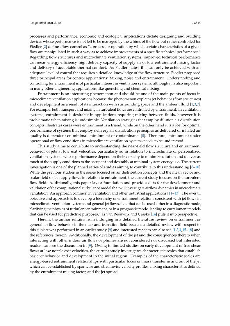
processes and performance, economic and ecological implications dictate designing and buildingdevices whose performance is not left to be managed by the whims of the flow but rather controlled for.Fiedler [2] defines flow control as “a process or operation by which certain characteristics of a givenflow are manipulated in such a way as to achieve improvements of a specific technical performance”.Regarding flow structures and microclimate ventilation systems, improved technical performancecan mean energy efficiency, high delivery capacity of supply air or low entrainment mixing factorand delivery of acceptable thermal comfort. As Fiedler states, this can only be achieved with anadequate level of control that requires a detailed knowledge of the flow structure. Fiedler proposedthree principal areas for control applications: Mixing, noise and entrainment. Understanding andcontrolling for entrainment is of particular interest in ventilation systems, although it is also importantin many other engineering applications like quenching and chemical mixing.

Entrainment is an interesting phenomenon and should be one of the main points of focus inmicroclimate ventilation applications because the phenomenon explains jet behavior (flow structures)and development as a result of its interaction with surrounding space and the ambient fluid [1,3,7].For example, both transport and mixing in turbulent flows are controlled by entrainment. In ventilationsystems, entrainment is desirable in applications requiring mixing between fluids, however it isproblematic when mixing is undesirable. Ventilation strategies that employ dilution air distributionconcepts illustrates cases were entrainment is a friend, while on the other hand it is a foe for optimalperformance of systems that employ delivery air distribution principles as delivered or inhaled airquality is dependent on minimal entrainment of contaminants [8]. Therefore, entrainment underoperational or flow conditions in microclimate ventilation systems needs to be understood.

This study aims to contribute to understanding the near-field flow structure and entrainmentbehavior of jets at low exit velocities, particularly so in relation to microclimate or personalizedventilation systems whose performance depend on their capacity to minimize dilution and deliver asmuch of the supply conditions to the occupant and desirably at minimal system energy use. The currentinvestigation is one of the planned series of studies aiming to contribute to this understanding [8–10].While the previous studies in the series focused on air distribution concepts and the mean vector andscalar field of jet supply flows in relation to entrainment, the current study focuses on the turbulentflow field. Additionally, this paper lays a foundation and provides data for the development andvalidation of the computational turbulence model that will investigate airflow dynamics in microclimateventilation. An approach common in ventilation and other industrial applications [11–13]. The overallobjective and approach is to develop a hierarchy of entrainment relations consistent with jet flows inmicroclimate ventilation systems and general jet flows, “ . . . that can be used either in a diagnostic mode,clarifying the physics of turbulent entrainment, or in a prognostic mode, leading to entrainment modelsthat can be used for predictive purposes,” as van Reeuwijk and Craske [14] puts it into perspective.

Herein, the author refrains from indulging in a detailed literature review on entrainment orgeneral jet flow behavior in the near and transition field because a detailed review with respect tothis subject was performed in an earlier study [9] and interested readers can also see [1,3,4,15–18] andthe references therein. Additionally, the development of the jet and the consequences thereto wheninteracting with other indoor air flows or plumes are not considered nor discussed but interestedreaders can see the discussion in [9]. Owing to limited studies on early development of free shearflows at low nozzle exit velocities, the current study investigates characteristic scales that establishbasic jet behavior and development in the initial region. Examples of the characteristic scales areenergy-based entrainment relationships with particular focus on mass transfer in and out of the jetwhich can be established by spanwise and streamwise velocity profiles, mixing characteristics definedby the entrainment mixing factor, and the jet spread.


2. Materials and Methods

2.1. Experimental Setup and Equipment

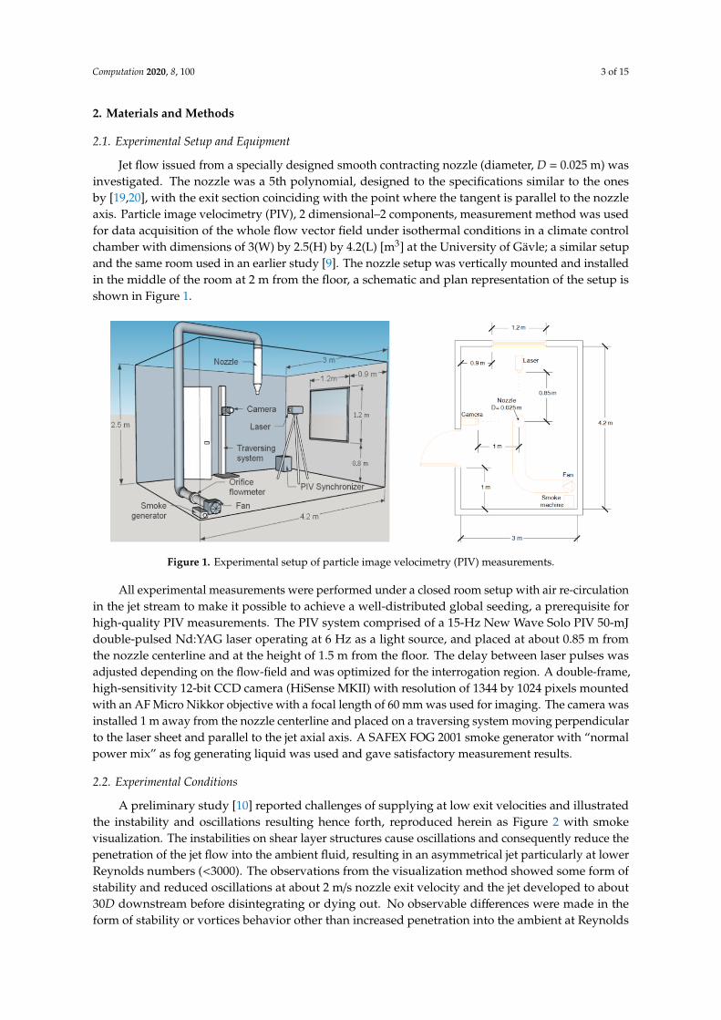
Jet flow issued from a specially designed smooth contracting nozzle (diameter, D = 0.025 m) wasinvestigated. The nozzle was a 5th polynomial, designed to the specifications similar to the onesby [19,20], with the exit section coinciding with the point where the tangent is parallel to the nozzleaxis. Particle image velocimetry (PIV), 2 dimensional–2 components, measurement method was usedfor data acquisition of the whole flow vector field under isothermal conditions in a climate controlchamber with dimensions of 3(W) by 2.5(H) by 4.2(L) [m3] at the University of Gävle; a similar setupand the same room used in an earlier study [9]. The nozzle setup was vertically mounted and installedin the middle of the room at 2 m from the floor, a schematic and plan representation of the setup isshown in Figure 1.

Computation 2020, 8, x FOR PEER REVIEW 3 of 15

2. Materials and Methods

2.1. Experimental Setup and Equipment

Jet flow issued from a specially designed smooth contracting nozzle (diameter, D = 0.025 m) was

investigated. The nozzle was a 5th polynomial, designed to the specifications similar to the ones by

[19,20], with the exit section coinciding with the point where the tangent is parallel to the nozzle axis.

Particle image velocimetry (PIV), 2 dimensional–2 components, measurement method was used for

data acquisition of the whole flow vector field under isothermal conditions in a climate control

chamber with dimensions of 3(W) by 2.5(H) by 4.2(L) [m3] at the University of Gävle; a similar setup

and the same room used in an earlier study [9]. The nozzle setup was vertically mounted and installed

in the middle of the room at 2 m from the floor, a schematic and plan representation of the setup is

shown in Figure 1.

All experimental measurements were performed under a closed room setup with air re-

circulation in the jet stream to make it possible to achieve a well-distributed global seeding, a

prerequisite for high-quality PIV measurements. The PIV system comprised of a 15-Hz New Wave

Solo PIV 50-mJ double-pulsed Nd:YAG laser operating at 6 Hz as a light source, and placed at about

0.85 m from the nozzle centerline and at the height of 1.5 m from the floor. The delay between laser

pulses was adjusted depending on the flow-field and was optimized for the interrogation region. A

double-frame, high-sensitivity 12-bit CCD camera (HiSense MKII) with resolution of 1344 by 1024

pixels mounted with an AF Micro Nikkor objective with a focal length of 60 mm was used for

imaging. The camera was installed 1 m away from the nozzle centerline and placed on a traversing

system moving perpendicular to the laser sheet and parallel to the jet axial axis. A SAFEX FOG 2001

smoke generator with “normal power mix” as fog generating liquid was used and gave satisfactory

measurement results.

Figure 1. Experimental setup of particle image velocimetry (PIV) measurements.

2.2. Experimental Conditions

A preliminary study [10] reported challenges of supplying at low exit velocities and illustrated

the instability and oscillations resulting hence forth, reproduced herein as Figure 2 with smoke

visualization. The instabilities on shear layer structures cause oscillations and consequently reduce

the penetration of the jet flow into the ambient fluid, resulting in an asymmetrical jet particularly at

lower Reynolds numbers (<3000). The observations from the visualization method showed some

form of stability and reduced oscillations at about 2 m/s nozzle exit velocity and the jet developed to

about 30D downstream before disintegrating or dying out. No observable differences were made in

the form of stability or vortices behavior other than increased penetration into the ambient at

Figure 1. Experimental setup of particle image velocimetry (PIV) measurements.

All experimental measurements were performed under a closed room setup with air re-circulationin the jet stream to make it possible to achieve a well-distributed global seeding, a prerequisite forhigh-quality PIV measurements. The PIV system comprised of a 15-Hz New Wave Solo PIV 50-mJdouble-pulsed Nd:YAG laser operating at 6 Hz as a light source, and placed at about 0.85 m fromthe nozzle centerline and at the height of 1.5 m from the floor. The delay between laser pulses wasadjusted depending on the flow-field and was optimized for the interrogation region. A double-frame,high-sensitivity 12-bit CCD camera (HiSense MKII) with resolution of 1344 by 1024 pixels mountedwith an AF Micro Nikkor objective with a focal length of 60 mm was used for imaging. The camera wasinstalled 1 m away from the nozzle centerline and placed on a traversing system moving perpendicularto the laser sheet and parallel to the jet axial axis. A SAFEX FOG 2001 smoke generator with “normalpower mix” as fog generating liquid was used and gave satisfactory measurement results.

2.2. Experimental Conditions

A preliminary study [10] reported challenges of supplying at low exit velocities and illustratedthe instability and oscillations resulting hence forth, reproduced herein as Figure 2 with smokevisualization. The instabilities on shear layer structures cause oscillations and consequently reduce thepenetration of the jet flow into the ambient fluid, resulting in an asymmetrical jet particularly at lowerReynolds numbers (<3000). The observations from the visualization method showed some form ofstability and reduced oscillations at about 2 m/s nozzle exit velocity and the jet developed to about30D downstream before disintegrating or dying out. No observable differences were made in theform of stability or vortices behavior other than increased penetration into the ambient at Reynolds


number ≥3400 (2.34 m/s nozzle exit velocity). Therefore, five experimental conditions were chosenfor the present study based on this insight, and on jet exit conditions similar to the range used undermicroclimate ventilation systems.


Reynolds number ≥3400 (2.34 m/s nozzle exit velocity). Therefore, five experimental conditions were

chosen for the present study based on this insight, and on jet exit conditions similar to the range used

under microclimate ventilation systems.

Figure 2. Jet development at different initial conditions.

The investigated experimental cases are listed in Table 1. The cases were defined by the Reynolds

number (Re) scaled with a relationship, Re = V0D/v, where V0 is the nozzle bulk exit velocity D is the

nozzle diameter and v is the kinematic viscosity of the fluid, v = 14.8 × 10‒6 m2/s [20]. The bulk exit

velocity was determined by the relationship V0 = 4𝑄/πD2, 𝑄 is the flowrate determined from a 25 mm

diameter orifice plate measurement meter.

Table 1. Experimental conditions.

Re 𝑸 (m3/s) V0 (m/s) 1

1 2000 0.00068 1.39

2 3400 0.00115 2.34

3 5600 0.00191 3.89

4 7600 0.00256 5.22

5 9300 0.00316 6.44 1 The bulk exit velocity.

Data acquisition and pre-processing was done with PIV software packages, Dantec Flow

manager and Dantec Dynamic Studio. The whole-field velocity vectors were obtained with three

interrogation regions limited to the measurement region 0 < x/D < 14. The cross-correlation was

performed with interrogation region of 32 by 32 pixels with a typical overlap of 50%. Peak and range

validation were applied to identify spurious vectors respective of the flow field. Overall, spurious

vectors were rejected and substituted with interpolated vectors within the spatial region in the mean

PIV field. PIV measurements uncertainties are influenced by various error sources, which can either

be systematic or statistical errors [21]. Statistical errors are mainly due to random sampling, [22–24]

while systematic errors relate to the experimental setup and procedure with likely sources of error

originating from tracking behavior, seeding density, background noise etc. Indoor airflow

measurements with 2 dimensional PIV have systematic errors less 2% [22,25]. For the current study,

the statistical errors were <8% in the time averaged velocity field using the central limit theorem [23].

The statistical mean velocity field was obtained with an ensemble of 650 images of instantaneous

velocity fields for each experimental case (spanwise (U) and streamwise (V) statistical means). The

turbulent velocity field was defined by the root mean square (r.m.s) of the fluctuations of the velocity

components (spanwise component u′; streamwise component 𝑣 ′) are compiled based on the

equations below, where u and 𝑣 are the spanwise and streamwise mean velocity whereas 𝑢̅ and 𝑣

are the variance of the velocity, respectively:

Figure 2. Jet development at different initial conditions.

The investigated experimental cases are listed in Table 1. The cases were defined by the Reynoldsnumber (Re) scaled with a relationship, Re = V0D/v, where V0 is the nozzle bulk exit velocity D is thenozzle diameter and v is the kinematic viscosity of the fluid, v = 14.8 × 10-6 m2/s [20]. The bulk exitvelocity was determined by the relationship V0 = 4Q/πD2, Q is the flowrate determined from a 25 mmdiameter orifice plate measurement meter.

Table 1. Experimental conditions.

Re Q(m3/s

)V0 (m/s) 1

1 2000 0.00068 1.392 3400 0.00115 2.343 5600 0.00191 3.894 7600 0.00256 5.225 9300 0.00316 6.44

1 The bulk exit velocity.

Data acquisition and pre-processing was done with PIV software packages, Dantec Flow managerand Dantec Dynamic Studio. The whole-field velocity vectors were obtained with three interrogationregions limited to the measurement region 0 < x/D < 14. The cross-correlation was performed withinterrogation region of 32 by 32 pixels with a typical overlap of 50%. Peak and range validationwere applied to identify spurious vectors respective of the flow field. Overall, spurious vectorswere rejected and substituted with interpolated vectors within the spatial region in the mean PIVfield. PIV measurements uncertainties are influenced by various error sources, which can either besystematic or statistical errors [21]. Statistical errors are mainly due to random sampling, [22–24] whilesystematic errors relate to the experimental setup and procedure with likely sources of error originatingfrom tracking behavior, seeding density, background noise etc. Indoor airflow measurements with 2dimensional PIV have systematic errors less 2% [22,25]. For the current study, the statistical errorswere <8% in the time averaged velocity field using the central limit theorem [23].

The statistical mean velocity field was obtained with an ensemble of 650 images of instantaneousvelocity fields for each experimental case (spanwise (U) and streamwise (V) statistical means).The turbulent velocity field was defined by the root mean square (r.m.s) of the fluctuations of thevelocity components (spanwise component u′; streamwise component v′) are compiled based on the


equations below, where u and v are the spanwise and streamwise mean velocity whereas u and v arethe variance of the velocity, respectively:

u′ =

√√1n

n∑i=1

(ui − u)2 (1)

v′ =

√√1n

n∑i=1

(vi − v)2 (2)

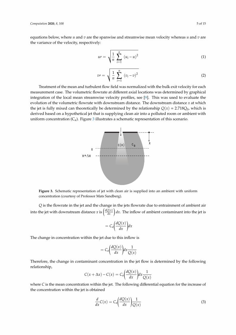
Treatment of the mean and turbulent flow field was normalized with the bulk exit velocity for eachmeasurement case. The volumetric flowrate at different axial locations was determined by graphicalintegration of the local mean streamwise velocity profiles, see [9]. This was used to evaluate theevolution of the volumetric flowrate with downstream distance. The downstream distance x at whichthe jet is fully mixed can theoretically be determined by the relationship Q(x) = 2.718Q0, which isderived based on a hypothetical jet that is supplying clean air into a polluted room or ambient withuniform concentration (Ca). Figure 3 illustrates a schematic representation of this scenario.


�́�̅ = √ 1

𝑛 ∑ 𝑛

𝑖=1 (𝑢̅𝑖 − 𝑢̅ )2 (1)

�́� = √ 1

𝑛 ∑ (𝑣𝑖 − 𝑣 )2

𝑛

𝑖=1 (2)

Treatment of the mean and turbulent flow field was normalized with the bulk exit velocity for

each measurement case. The volumetric flowrate at different axial locations was determined by

graphical integration of the local mean streamwise velocity profiles, see [9]. This was used to evaluate

the evolution of the volumetric flowrate with downstream distance. The downstream distance x at

which the jet is fully mixed can theoretically be determined by the relationship 𝑄(𝑥) = 2.718𝑄0,

which is derived based on a hypothetical jet that is supplying clean air into a polluted room or

ambient with uniform concentration (Ca). Figure 3 illustrates a schematic representation of this

scenario.

Figure 3. Schematic representation of jet with clean air is supplied into an ambient with uniform

concentration (courtesy of Professor Mats Sandberg).

𝑄 is the flowrate in the jet and the change in the jets flowrate due to entrainment of ambient air

into the jet with downstream distance x is (𝑑𝑄(𝑥)

𝑑𝑥) 𝑑𝑥. The inflow of ambient contaminant into the jet

is

= 𝐶𝑎(𝑑𝑄(𝑥)

𝑑𝑥)𝑑𝑥

The change in concentration within the jet due to this inflow is

= 𝐶𝑎(𝑑𝑄(𝑥)

𝑑𝑥)𝑑𝑥

1

𝑄(𝑥)

Therefore, the change in contaminant concentration in the jet flow is determined by the following

relationship,

𝐶(𝑥 + ∆𝑥) − 𝐶(𝑥) = 𝐶𝑎(𝑑𝑄(𝑥)

𝑑𝑥)𝑑𝑥

1

𝑄(𝑥)

where C is the mean concentration within the jet. The following differential equation for the increase

of the concentration within the jet is obtained

𝑑

𝑑𝑥𝐶(𝑥) = 𝐶𝑎(

𝑑𝑄(𝑥)

𝑑𝑥)

1

𝑄(𝑥) (3)

After integration of Equation (3) we obtain

𝐶(𝑥) − 𝐶(0) = 𝐶𝑎∫(𝑑𝑄(𝑥)

𝑑𝑥)

1

𝑄(𝑥)𝑑𝑥

𝑥

0

(4)

The integral is

Figure 3. Schematic representation of jet with clean air is supplied into an ambient with uniformconcentration (courtesy of Professor Mats Sandberg).

Q is the flowrate in the jet and the change in the jets flowrate due to entrainment of ambient air

into the jet with downstream distance x is(

dQ(x)dx

)dx. The inflow of ambient contaminant into the jet is

= Ca

(dQ(x)

dx

)dx

The change in concentration within the jet due to this inflow is

= Ca

(dQ(x)

dx

)dx

1Q(x)

Therefore, the change in contaminant concentration in the jet flow is determined by the followingrelationship,

C(x + ∆x) −C(x) = Ca

(dQ(x)

dx

)dx

1Q(x)

where C is the mean concentration within the jet. The following differential equation for the increase ofthe concentration within the jet is obtained

ddx

C(x) = Ca

(dQ(x)

dx

)1

Q(x)(3)


After integration of Equation (3) we obtain

C(x) −C(0) = Ca

x∫0

(dQ(x)

dx

)1

Q(x)dx (4)

The integral isx∫

0

(dQ(x)

dx

)1

Q(x)dx = ln Q(x) − ln Q(0) = ln

Q(x)Q(0)

(5)

Assuming that the initial concentration at the exit in the jet in relation to the ambient contaminant iszero, C(0) = 0, Equation (4) is simplified to

C(x)Ca

= lnQ(x)Q(0)

(6)

Setting the downstream distance x to be the distance where the concentration in the jet has becomeequal to the concentration in the ambient, C(x) = Ca.

lnQ(x)Q(0)

= 1 (7)

This gives the ratio between the flow rate at location x, where the contaminant concentration in the jetis equal to the concentration of the ambient, and the flowrate at the nozzle exit to be

Q(x)Q(0)

= 2.718 (8)

Thus, if the evolution of the volumetric flowrate with downstream distance is established, one cansolve for the hypothetical distance at which the concentration in the jet is equal to that of the room.

3. Results

3.1. Evolution of the Mean Velocity Field

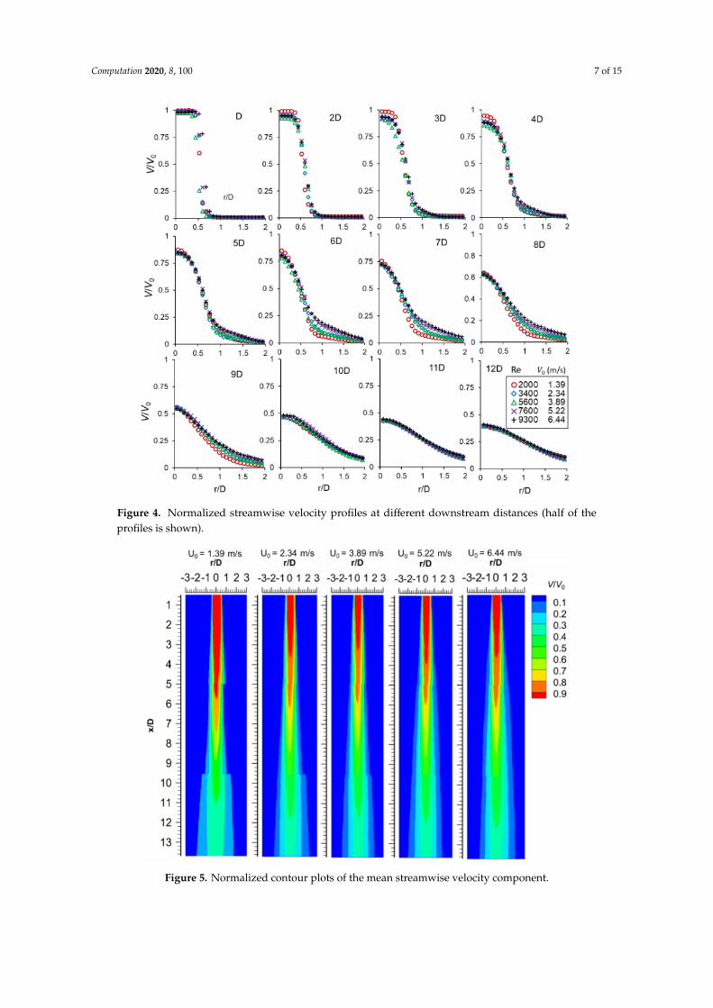
A time averaged quantitative characterization of the streamwise velocity profiles are presented inFigure 4 and, as observed, in all cases a top-hat profile typical of free round jets [26–28] was obtained.The exit top-hat velocity profiles diffused out gradually to a Gaussian profile within the first fourdiameters and with increase in downstream distance the velocity distribution eventually relaxes tobell-shaped profiles [29]. An apparent observation is that the velocity profiles are superimposed oneach other up to 4D, with the exception of the case with the lowest nozzle exit velocity (sustains theexit velocity longer than other cases). After the zone of flow establishment, the Reynolds numberdependence manifests between six to nine diameters which may be deduced as part of a criticaltransitional region where the jet changes from laminar to turbulent flow. Here, increase in exit velocitiessuggest increase in the radial spread (width of the jet) with downstream distance. However, after 10Dthe profiles exhibit self-similarity as they are superimposed on each other again for the rest of theinterrogation region (shown here only up to 12D). This observation is supported by the qualitativerepresentation of the mean flow field shown in Figure 5.

Computation 2020, 8, 100 7 of 15Computation 2020, 8, x FOR PEER REVIEW 7 of 15

Figure 4. Normalized streamwise velocity profiles at different downstream distances (half of the

profiles is shown).

Figure 5. Normalized contour plots of the mean streamwise velocity component.

Figure 4. Normalized streamwise velocity profiles at different downstream distances (half of theprofiles is shown).


Figure 4. Normalized streamwise velocity profiles at different downstream distances (half of the

profiles is shown).

Figure 5. Normalized contour plots of the mean streamwise velocity component. Figure 5. Normalized contour plots of the mean streamwise velocity component.


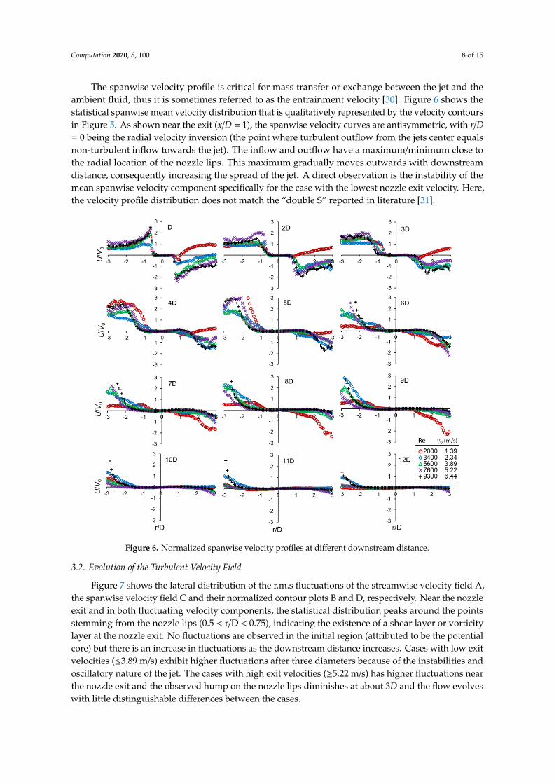
The spanwise velocity profile is critical for mass transfer or exchange between the jet and theambient fluid, thus it is sometimes referred to as the entrainment velocity [30]. Figure 6 shows thestatistical spanwise mean velocity distribution that is qualitatively represented by the velocity contoursin Figure 5. As shown near the exit (x/D = 1), the spanwise velocity curves are antisymmetric, with r/D= 0 being the radial velocity inversion (the point where turbulent outflow from the jets center equalsnon-turbulent inflow towards the jet). The inflow and outflow have a maximum/minimum close tothe radial location of the nozzle lips. This maximum gradually moves outwards with downstreamdistance, consequently increasing the spread of the jet. A direct observation is the instability of themean spanwise velocity component specifically for the case with the lowest nozzle exit velocity. Here,the velocity profile distribution does not match the “double S” reported in literature [31].Computation 2020, 8, x FOR PEER REVIEW 8 of 15

Figure 6. Normalized spanwise velocity profiles at different downstream distance.

3.2. Evolution of the Turbulent Velocity Field

Figure 7 shows the lateral distribution of the r.m.s fluctuations of the streamwise velocity field

A, the spanwise velocity field C and their normalized contour plots B and D, respectively. Near the

nozzle exit and in both fluctuating velocity components, the statistical distribution peaks around the

points stemming from the nozzle lips (0.5 < r/D < 0.75), indicating the existence of a shear layer or

vorticity layer at the nozzle exit. No fluctuations are observed in the initial region (attributed to be

the potential core) but there is an increase in fluctuations as the downstream distance increases. Cases

with low exit velocities (≤3.89 m/s) exhibit higher fluctuations after three diameters because of the

instabilities and oscillatory nature of the jet. The cases with high exit velocities (≥5.22 m/s) has higher

fluctuations near the nozzle exit and the observed hump on the nozzle lips diminishes at about 3D

and the flow evolves with little distinguishable differences between the cases.

The contour plots show that the streamwise r.m.s fluctuations (𝑣′) peaks in the jet mixing layer

along the nozzle lips (about r/D ≈ 0.5) and grows stronger towards the nozzle exit with increasing

exit velocity. In setups with V0 ≥ 5.22 m/s, a strong jet mixing layer is uniformly sustained downstream

up to about x/D = 7 after which it gradually disintegrates to an asymptotic flow. Similarly, the

spanwise r.m.s fluctuations (u′) peaks along the nozzle lips but the fluctuations grow inwards

towards the jet centerline. In both Figure 7B,D, the inward growth and merging of the shear layer

introduce fluctuations along the central portion of the jet consequently increasing entrainment and

the mixing processes between the jet and the ambient.

Figure 6. Normalized spanwise velocity profiles at different downstream distance.

3.2. Evolution of the Turbulent Velocity Field

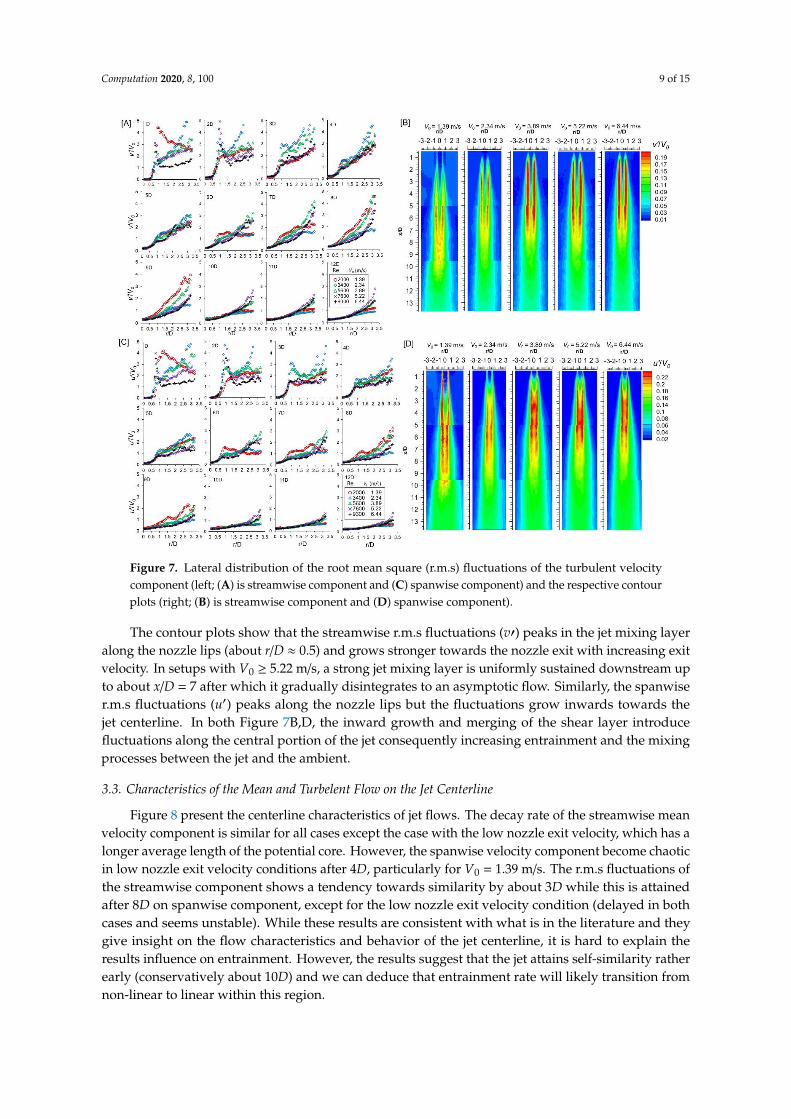
Figure 7 shows the lateral distribution of the r.m.s fluctuations of the streamwise velocity field A,the spanwise velocity field C and their normalized contour plots B and D, respectively. Near the nozzleexit and in both fluctuating velocity components, the statistical distribution peaks around the pointsstemming from the nozzle lips (0.5 < r/D < 0.75), indicating the existence of a shear layer or vorticitylayer at the nozzle exit. No fluctuations are observed in the initial region (attributed to be the potentialcore) but there is an increase in fluctuations as the downstream distance increases. Cases with low exitvelocities (≤3.89 m/s) exhibit higher fluctuations after three diameters because of the instabilities andoscillatory nature of the jet. The cases with high exit velocities (≥5.22 m/s) has higher fluctuations nearthe nozzle exit and the observed hump on the nozzle lips diminishes at about 3D and the flow evolveswith little distinguishable differences between the cases.



Figure 7. Lateral distribution of the root mean square (r.m.s) fluctuations of the turbulent velocity

component (left; (A) is streamwise component and (C) spanwise component) and the respective

contour plots (right; (B) is streamwise component and (D) spanwise component).

3.3. Characteristics of the Mean and Turbelent Flow on the Jet Centerline

Figure 8 present the centerline characteristics of jet flows. The decay rate of the streamwise mean

velocity component is similar for all cases except the case with the low nozzle exit velocity, which has

a longer average length of the potential core. However, the spanwise velocity component become

chaotic in low nozzle exit velocity conditions after 4D, particularly for V0 = 1.39 m/s. The r.m.s

fluctuations of the streamwise component shows a tendency towards similarity by about 3D while

this is attained after 8D on spanwise component, except for the low nozzle exit velocity condition

(delayed in both cases and seems unstable). While these results are consistent with what is in the

literature and they give insight on the flow characteristics and behavior of the jet centerline, it is hard

to explain the results influence on entrainment. However, the results suggest that the jet attains self-

similarity rather early (conservatively about 10D) and we can deduce that entrainment rate will likely

transition from non-linear to linear within this region.

3.4. Evolution of the Mass Flowrate and Jet Entrainment

When the jet entrains fluid from outside the jet boundaries into the main turbulent stream, the

volumetric mass flowrate increases with increasing downstream distance from the jet exit [32]. Figure

9 shows the change of the volumetric flowrate with downstream distance. The volumetric flowrate

in the near field develops nonlinearly and depend on the exit velocity reaches a constant within the

first 4D. In higher exit velocity flows, there is a sharp increase in volumetric flowrate and quickly

reaches a constant as compared to flows with low exit velocities. The general overview shows that

conditions with high exit flows have low mass flowrate increase which is a consequence of low

entrainment compared to conditions with low nozzle exit velocities.

Figure 7. Lateral distribution of the root mean square (r.m.s) fluctuations of the turbulent velocitycomponent (left; (A) is streamwise component and (C) spanwise component) and the respective contourplots (right; (B) is streamwise component and (D) spanwise component).

The contour plots show that the streamwise r.m.s fluctuations (v′) peaks in the jet mixing layeralong the nozzle lips (about r/D ≈ 0.5) and grows stronger towards the nozzle exit with increasing exitvelocity. In setups with V0 ≥ 5.22 m/s, a strong jet mixing layer is uniformly sustained downstream upto about x/D = 7 after which it gradually disintegrates to an asymptotic flow. Similarly, the spanwiser.m.s fluctuations (u′) peaks along the nozzle lips but the fluctuations grow inwards towards thejet centerline. In both Figure 7B,D, the inward growth and merging of the shear layer introducefluctuations along the central portion of the jet consequently increasing entrainment and the mixingprocesses between the jet and the ambient.

3.3. Characteristics of the Mean and Turbelent Flow on the Jet Centerline

Figure 8 present the centerline characteristics of jet flows. The decay rate of the streamwise meanvelocity component is similar for all cases except the case with the low nozzle exit velocity, which has alonger average length of the potential core. However, the spanwise velocity component become chaoticin low nozzle exit velocity conditions after 4D, particularly for V0 = 1.39 m/s. The r.m.s fluctuations ofthe streamwise component shows a tendency towards similarity by about 3D while this is attainedafter 8D on spanwise component, except for the low nozzle exit velocity condition (delayed in bothcases and seems unstable). While these results are consistent with what is in the literature and theygive insight on the flow characteristics and behavior of the jet centerline, it is hard to explain theresults influence on entrainment. However, the results suggest that the jet attains self-similarity ratherearly (conservatively about 10D) and we can deduce that entrainment rate will likely transition fromnon-linear to linear within this region.


Figure 8. Centerline characteristics of mean and turbulent flow field.

Figure 9. Volumetric flowrate as a function of downstream distance.

The most effective way to characterize this behavior is to plot the instantaneous vector contour

field which characterizes vortex structures. Figure 10 offers a qualitative interpretation of the

instantaneous flow field (V0 = 5.22 m/s and V0 = 6.44 m/s had no distinct differences). As

comprehensively described by List [33], when a high speed jet interacts with the irrotational ambient

fluid, a laminar shear layer is produced. The shear layer is unstable and grows very rapidly, forming

coherent structures (ring vortices) that pair and rotate along the jets axis and later break off after a

loss of momentum (increased mixing happens after break off). This behavior of coherent structures

increases mass exchange of fluids between turbulent jet fluid and the irrotational ambient fluid.

The main factor governing the resulting nature of the flow is the momentum flow [8]. The

instantaneous contour plots show that the conditions with low nozzle exit velocities (V0 = 1.39 m/s

and V0 = 2.34 m/s) are oscillatory and with minimal to no coherent structures on the shear layer

(particularly for V0 = 1.39 m/s). The oscillating manner of the jet creates flow instabilities as also

evidenced in an earlier study [10]. In low nozzle exit velocity cases, the momentum flow is insufficient

to generate and sustain the flow of coherent structures, thus any vortices or tendency of formation

easily disintegrate within a short downstream distance from the nozzle exit (about x/D = 3). Cases

with high nozzle exit velocities are dominated by formation of small-scale vortices close to the nozzle

exit (x/D = 1; suggesting early mixing of the jet flow) which later disintegrate downstream at about

x/D = 5. This behavior explains the evolution of the volumetric mass flowrate.


3.4. Evolution of the Mass Flowrate and Jet Entrainment

When the jet entrains fluid from outside the jet boundaries into the main turbulent stream,the volumetric mass flowrate increases with increasing downstream distance from the jet exit [32].Figure 9 shows the change of the volumetric flowrate with downstream distance. The volumetricflowrate in the near field develops nonlinearly and depend on the exit velocity reaches a constantwithin the first 4D. In higher exit velocity flows, there is a sharp increase in volumetric flowrate andquickly reaches a constant as compared to flows with low exit velocities. The general overview showsthat conditions with high exit flows have low mass flowrate increase which is a consequence of lowentrainment compared to conditions with low nozzle exit velocities.




The most effective way to characterize this behavior is to plot the instantaneous vector contour

field which characterizes vortex structures. Figure 10 offers a qualitative interpretation of the

instantaneous flow field (V0 = 5.22 m/s and V0 = 6.44 m/s had no distinct differences). As

comprehensively described by List [33], when a high speed jet interacts with the irrotational ambient

fluid, a laminar shear layer is produced. The shear layer is unstable and grows very rapidly, forming

coherent structures (ring vortices) that pair and rotate along the jets axis and later break off after a

loss of momentum (increased mixing happens after break off). This behavior of coherent structures

increases mass exchange of fluids between turbulent jet fluid and the irrotational ambient fluid.

The main factor governing the resulting nature of the flow is the momentum flow [8]. The

instantaneous contour plots show that the conditions with low nozzle exit velocities (V0 = 1.39 m/s

and V0 = 2.34 m/s) are oscillatory and with minimal to no coherent structures on the shear layer

(particularly for V0 = 1.39 m/s). The oscillating manner of the jet creates flow instabilities as also

evidenced in an earlier study [10]. In low nozzle exit velocity cases, the momentum flow is insufficient

to generate and sustain the flow of coherent structures, thus any vortices or tendency of formation

easily disintegrate within a short downstream distance from the nozzle exit (about x/D = 3). Cases

with high nozzle exit velocities are dominated by formation of small-scale vortices close to the nozzle

exit (x/D = 1; suggesting early mixing of the jet flow) which later disintegrate downstream at about

x/D = 5. This behavior explains the evolution of the volumetric mass flowrate.


The most effective way to characterize this behavior is to plot the instantaneous vector contour fieldwhich characterizes vortex structures. Figure 10 offers a qualitative interpretation of the instantaneousflow field (V0 = 5.22 m/s and V0 = 6.44 m/s had no distinct differences). As comprehensively describedby List [33], when a high speed jet interacts with the irrotational ambient fluid, a laminar shearlayer is produced. The shear layer is unstable and grows very rapidly, forming coherent structures(ring vortices) that pair and rotate along the jets axis and later break off after a loss of momentum(increased mixing happens after break off). This behavior of coherent structures increases massexchange of fluids between turbulent jet fluid and the irrotational ambient fluid.


Figure 10. Instantaneous velocity fields with velocity vectors, streamlines and contours of their

magnitudes. These images are selected arbitrarily out of 650 images and presented here as typical

flow for each experimental condition.

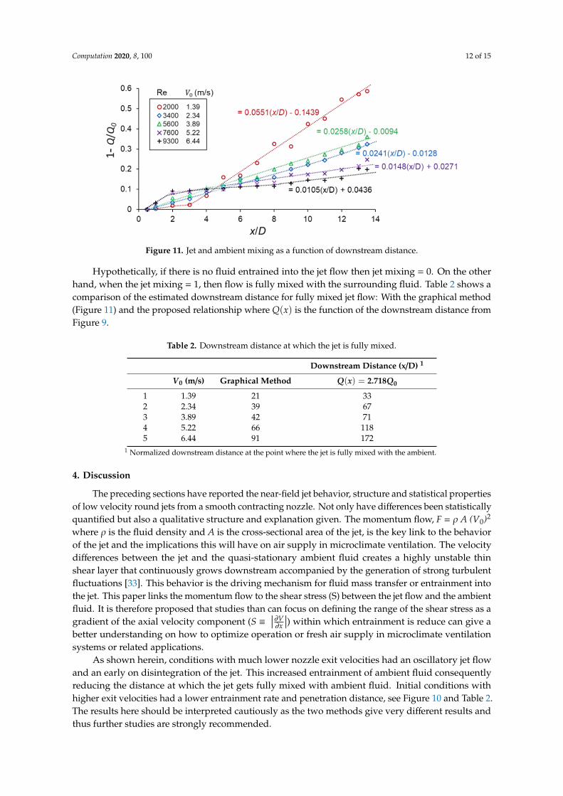
As the jet develop downstream, mixing between the ambient and the jet stream occurs. Figure

11 shows the jet and ambient mixing as a function of downstream distance. Logically, as shown, the

mixing of the flow follows the evolution of the volumetric flowrate as a function of downstream

distance (compare Figure 9). The general observation is that when the profiles attain linearity, mixing

reduces with increasing nozzle exit velocities (except for V0 = 3.89 m/s which develops similarly to V0

= 2.34 m/s, no explanation was found for this case).

Figure 11. Jet and ambient mixing as a function of downstream distance.

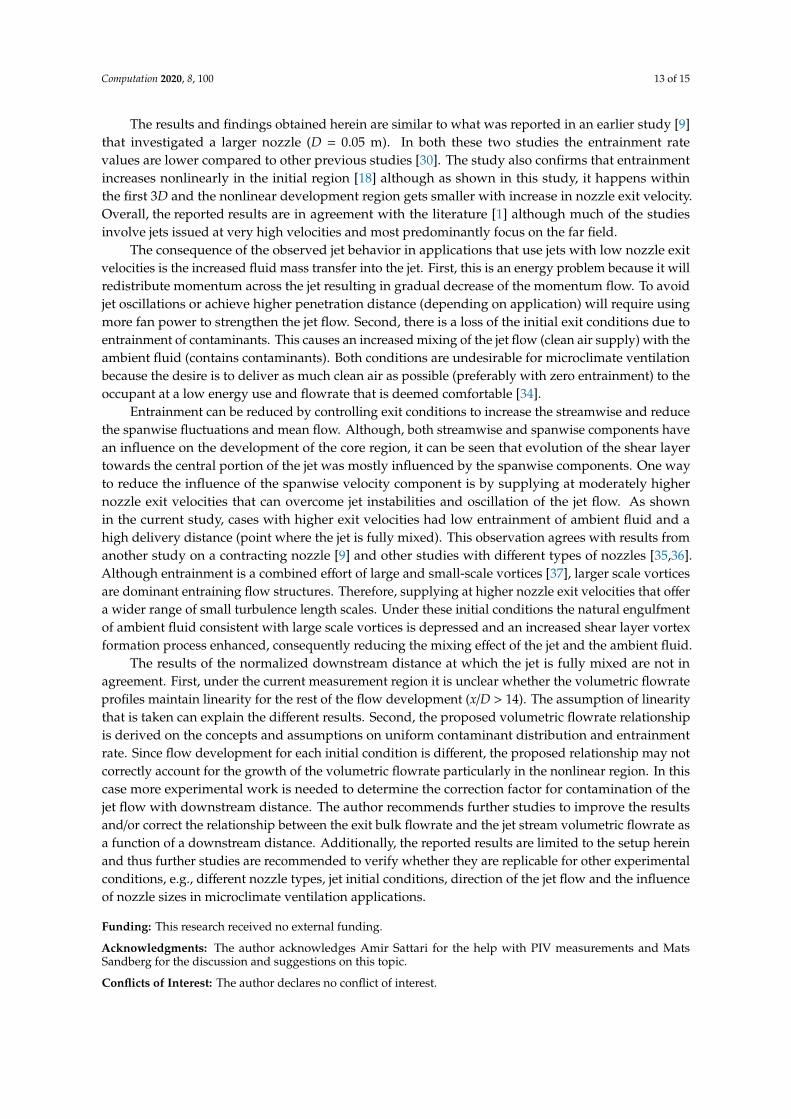
Hypothetically, if there is no fluid entrained into the jet flow then jet mixing = 0. On the other

hand, when the jet mixing = 1, then flow is fully mixed with the surrounding fluid. Table 2 shows a

comparison of the estimated downstream distance for fully mixed jet flow: With the graphical

method (Figure 11) and the proposed relationship where 𝑄(𝑥) is the function of the downstream

distance from Figure 9.

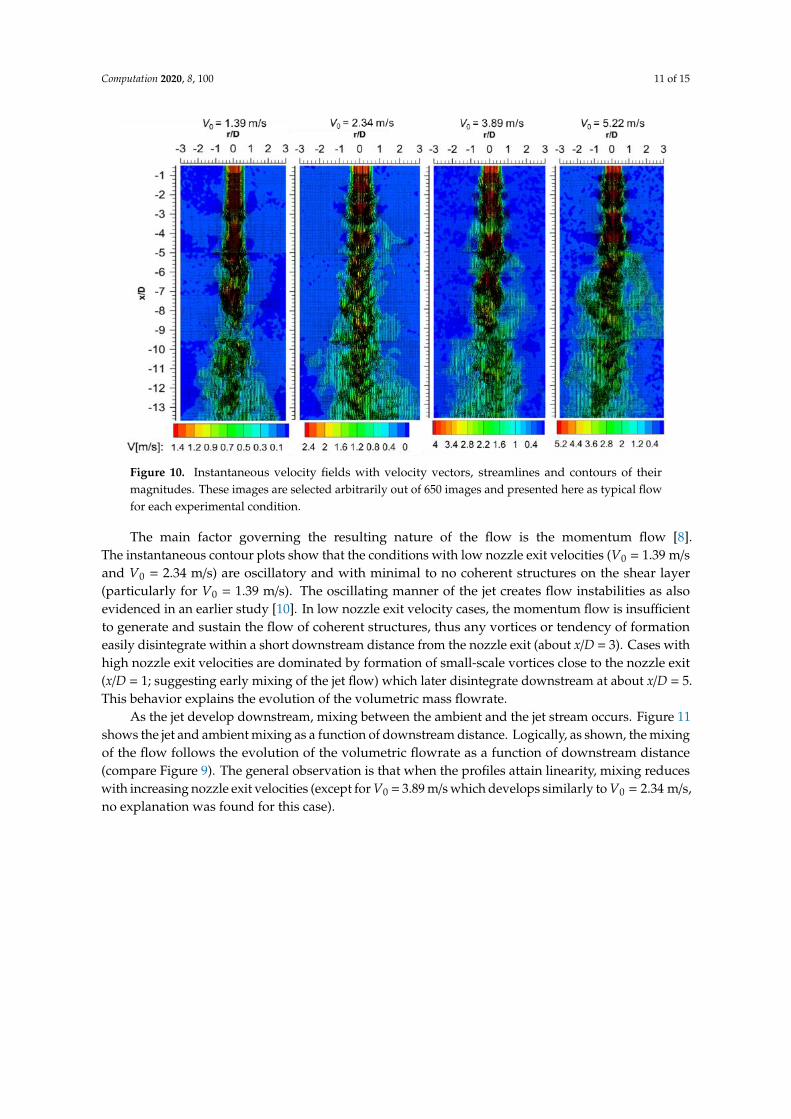
Figure 10. Instantaneous velocity fields with velocity vectors, streamlines and contours of theirmagnitudes. These images are selected arbitrarily out of 650 images and presented here as typical flowfor each experimental condition.

The main factor governing the resulting nature of the flow is the momentum flow [8].The instantaneous contour plots show that the conditions with low nozzle exit velocities (V0 = 1.39 m/sand V0 = 2.34 m/s) are oscillatory and with minimal to no coherent structures on the shear layer(particularly for V0 = 1.39 m/s). The oscillating manner of the jet creates flow instabilities as alsoevidenced in an earlier study [10]. In low nozzle exit velocity cases, the momentum flow is insufficientto generate and sustain the flow of coherent structures, thus any vortices or tendency of formationeasily disintegrate within a short downstream distance from the nozzle exit (about x/D = 3). Cases withhigh nozzle exit velocities are dominated by formation of small-scale vortices close to the nozzle exit(x/D = 1; suggesting early mixing of the jet flow) which later disintegrate downstream at about x/D = 5.This behavior explains the evolution of the volumetric mass flowrate.

As the jet develop downstream, mixing between the ambient and the jet stream occurs. Figure 11shows the jet and ambient mixing as a function of downstream distance. Logically, as shown, the mixingof the flow follows the evolution of the volumetric flowrate as a function of downstream distance(compare Figure 9). The general observation is that when the profiles attain linearity, mixing reduceswith increasing nozzle exit velocities (except for V0 = 3.89 m/s which develops similarly to V0 = 2.34 m/s,no explanation was found for this case).

Computation 2020, 8, 100 12 of 15


Figure 10. Instantaneous velocity fields with velocity vectors, streamlines and contours of their

magnitudes. These images are selected arbitrarily out of 650 images and presented here as typical

flow for each experimental condition.

As the jet develop downstream, mixing between the ambient and the jet stream occurs. Figure

11 shows the jet and ambient mixing as a function of downstream distance. Logically, as shown, the

mixing of the flow follows the evolution of the volumetric flowrate as a function of downstream

distance (compare Figure 9). The general observation is that when the profiles attain linearity, mixing

reduces with increasing nozzle exit velocities (except for V0 = 3.89 m/s which develops similarly to V0

= 2.34 m/s, no explanation was found for this case).


Hypothetically, if there is no fluid entrained into the jet flow then jet mixing = 0. On the other

hand, when the jet mixing = 1, then flow is fully mixed with the surrounding fluid. Table 2 shows a

comparison of the estimated downstream distance for fully mixed jet flow: With the graphical

method (Figure 11) and the proposed relationship where 𝑄(𝑥) is the function of the downstream

distance from Figure 9.


Hypothetically, if there is no fluid entrained into the jet flow then jet mixing = 0. On the otherhand, when the jet mixing = 1, then flow is fully mixed with the surrounding fluid. Table 2 shows acomparison of the estimated downstream distance for fully mixed jet flow: With the graphical method(Figure 11) and the proposed relationship where Q(x) is the function of the downstream distance fromFigure 9.

Table 2. Downstream distance at which the jet is fully mixed.

Downstream Distance (x/D) 1

V0 (m/s) Graphical Method Q(x) = 2.718Q0

1 1.39 21 332 2.34 39 673 3.89 42 714 5.22 66 1185 6.44 91 172

1 Normalized downstream distance at the point where the jet is fully mixed with the ambient.

4. Discussion

The preceding sections have reported the near-field jet behavior, structure and statistical propertiesof low velocity round jets from a smooth contracting nozzle. Not only have differences been statisticallyquantified but also a qualitative structure and explanation given. The momentum flow, F = ρ A (V0)2

where ρ is the fluid density and A is the cross-sectional area of the jet, is the key link to the behaviorof the jet and the implications this will have on air supply in microclimate ventilation. The velocitydifferences between the jet and the quasi-stationary ambient fluid creates a highly unstable thinshear layer that continuously grows downstream accompanied by the generation of strong turbulentfluctuations [33]. This behavior is the driving mechanism for fluid mass transfer or entrainment intothe jet. This paper links the momentum flow to the shear stress (S) between the jet flow and the ambientfluid. It is therefore proposed that studies than can focus on defining the range of the shear stress as agradient of the axial velocity component (S ≡

∣∣∣∂V∂x

∣∣∣) within which entrainment is reduce can give abetter understanding on how to optimize operation or fresh air supply in microclimate ventilationsystems or related applications.

As shown herein, conditions with much lower nozzle exit velocities had an oscillatory jet flowand an early on disintegration of the jet. This increased entrainment of ambient fluid consequentlyreducing the distance at which the jet gets fully mixed with ambient fluid. Initial conditions withhigher exit velocities had a lower entrainment rate and penetration distance, see Figure 10 and Table 2.The results here should be interpreted cautiously as the two methods give very different results andthus further studies are strongly recommended.

Computation 2020, 8, 100 13 of 15

The results and findings obtained herein are similar to what was reported in an earlier study [9]that investigated a larger nozzle (D = 0.05 m). In both these two studies the entrainment ratevalues are lower compared to other previous studies [30]. The study also confirms that entrainmentincreases nonlinearly in the initial region [18] although as shown in this study, it happens withinthe first 3D and the nonlinear development region gets smaller with increase in nozzle exit velocity.Overall, the reported results are in agreement with the literature [1] although much of the studiesinvolve jets issued at very high velocities and most predominantly focus on the far field.

The consequence of the observed jet behavior in applications that use jets with low nozzle exitvelocities is the increased fluid mass transfer into the jet. First, this is an energy problem because it willredistribute momentum across the jet resulting in gradual decrease of the momentum flow. To avoidjet oscillations or achieve higher penetration distance (depending on application) will require usingmore fan power to strengthen the jet flow. Second, there is a loss of the initial exit conditions due toentrainment of contaminants. This causes an increased mixing of the jet flow (clean air supply) with theambient fluid (contains contaminants). Both conditions are undesirable for microclimate ventilationbecause the desire is to deliver as much clean air as possible (preferably with zero entrainment) to theoccupant at a low energy use and flowrate that is deemed comfortable [34].

Entrainment can be reduced by controlling exit conditions to increase the streamwise and reducethe spanwise fluctuations and mean flow. Although, both streamwise and spanwise components havean influence on the development of the core region, it can be seen that evolution of the shear layertowards the central portion of the jet was mostly influenced by the spanwise components. One wayto reduce the influence of the spanwise velocity component is by supplying at moderately highernozzle exit velocities that can overcome jet instabilities and oscillation of the jet flow. As shownin the current study, cases with higher exit velocities had low entrainment of ambient fluid and ahigh delivery distance (point where the jet is fully mixed). This observation agrees with results fromanother study on a contracting nozzle [9] and other studies with different types of nozzles [35,36].Although entrainment is a combined effort of large and small-scale vortices [37], larger scale vorticesare dominant entraining flow structures. Therefore, supplying at higher nozzle exit velocities that offera wider range of small turbulence length scales. Under these initial conditions the natural engulfmentof ambient fluid consistent with large scale vortices is depressed and an increased shear layer vortexformation process enhanced, consequently reducing the mixing effect of the jet and the ambient fluid.

The results of the normalized downstream distance at which the jet is fully mixed are not inagreement. First, under the current measurement region it is unclear whether the volumetric flowrateprofiles maintain linearity for the rest of the flow development (x/D > 14). The assumption of linearitythat is taken can explain the different results. Second, the proposed volumetric flowrate relationshipis derived on the concepts and assumptions on uniform contaminant distribution and entrainmentrate. Since flow development for each initial condition is different, the proposed relationship may notcorrectly account for the growth of the volumetric flowrate particularly in the nonlinear region. In thiscase more experimental work is needed to determine the correction factor for contamination of thejet flow with downstream distance. The author recommends further studies to improve the resultsand/or correct the relationship between the exit bulk flowrate and the jet stream volumetric flowrate asa function of a downstream distance. Additionally, the reported results are limited to the setup hereinand thus further studies are recommended to verify whether they are replicable for other experimentalconditions, e.g., different nozzle types, jet initial conditions, direction of the jet flow and the influenceof nozzle sizes in microclimate ventilation applications.

Funding: This research received no external funding.

Acknowledgments: The author acknowledges Amir Sattari for the help with PIV measurements and MatsSandberg for the discussion and suggestions on this topic.

Conflicts of Interest: The author declares no conflict of interest.

Computation 2020, 8, 100 14 of 15

Appendix A

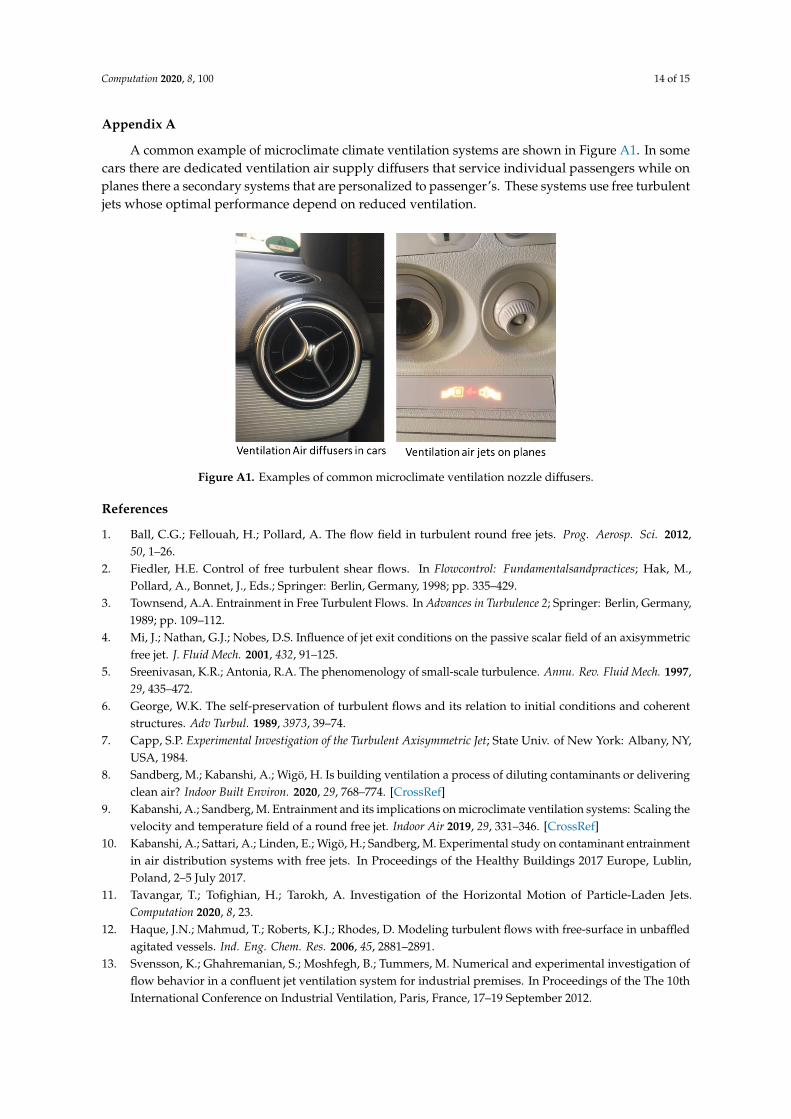
A common example of microclimate climate ventilation systems are shown in Figure A1. In somecars there are dedicated ventilation air supply diffusers that service individual passengers while onplanes there a secondary systems that are personalized to passenger’s. These systems use free turbulentjets whose optimal performance depend on reduced ventilation.


nozzle exit velocities that can overcome jet instabilities and oscillation of the jet flow. As shown in

the current study, cases with higher exit velocities had low entrainment of ambient fluid and a high

delivery distance (point where the jet is fully mixed). This observation agrees with results from

another study on a contracting nozzle [9] and other studies with different types of nozzles [35,36].

Although entrainment is a combined effort of large and small-scale vortices [37], larger scale vortices

are dominant entraining flow structures. Therefore, supplying at higher nozzle exit velocities that

offer a wider range of small turbulence length scales. Under these initial conditions the natural

engulfment of ambient fluid consistent with large scale vortices is depressed and an increased shear

layer vortex formation process enhanced, consequently reducing the mixing effect of the jet and the

ambient fluid.

The results of the normalized downstream distance at which the jet is fully mixed are not in

agreement. First, under the current measurement region it is unclear whether the volumetric flowrate

profiles maintain linearity for the rest of the flow development (x/D > 14). The assumption of linearity

that is taken can explain the different results. Second, the proposed volumetric flowrate relationship

is derived on the concepts and assumptions on uniform contaminant distribution and entrainment

rate. Since flow development for each initial condition is different, the proposed relationship may not

correctly account for the growth of the volumetric flowrate particularly in the nonlinear region. In

this case more experimental work is needed to determine the correction factor for contamination of

the jet flow with downstream distance. The author recommends further studies to improve the results

and/or correct the relationship between the exit bulk flowrate and the jet stream volumetric flowrate

as a function of a downstream distance. Additionally, the reported results are limited to the setup

herein and thus further studies are recommended to verify whether they are replicable for other

experimental conditions, e.g., different nozzle types, jet initial conditions, direction of the jet flow and

the influence of nozzle sizes in microclimate ventilation applications.

Funding: This research received no external funding.

Acknowledgments: The author acknowledges Amir Sattari for the help with PIV measurements and Mats

Sandberg for the discussion and suggestions on this topic.

Conflicts of Interest: The author declares no conflict of interest.

Appendix A

A common example of microclimate climate ventilation systems are shown in Figure A1. In some

cars there are dedicated ventilation air supply diffusers that service individual passengers while on

planes there a secondary systems that are personalized to passenger’s. These systems use free

turbulent jets whose optimal performance depend on reduced ventilation.

Figure A1. Examples of common microclimate ventilation nozzle diffusers.

Figure A1. Examples of common microclimate ventilation nozzle diffusers.

References

1. Ball, C.G.; Fellouah, H.; Pollard, A. The flow field in turbulent round free jets. Prog. Aerosp. Sci. 2012,50, 1–26.

2. Fiedler, H.E. Control of free turbulent shear flows. In Flowcontrol: Fundamentalsandpractices; Hak, M.,Pollard, A., Bonnet, J., Eds.; Springer: Berlin, Germany, 1998; pp. 335–429.

3. Townsend, A.A. Entrainment in Free Turbulent Flows. In Advances in Turbulence 2; Springer: Berlin, Germany,1989; pp. 109–112.

4. Mi, J.; Nathan, G.J.; Nobes, D.S. Influence of jet exit conditions on the passive scalar field of an axisymmetricfree jet. J. Fluid Mech. 2001, 432, 91–125.

5. Sreenivasan, K.R.; Antonia, R.A. The phenomenology of small-scale turbulence. Annu. Rev. Fluid Mech. 1997,29, 435–472.

6. George, W.K. The self-preservation of turbulent flows and its relation to initial conditions and coherentstructures. Adv Turbul. 1989, 3973, 39–74.

7. Capp, S.P. Experimental Investigation of the Turbulent Axisymmetric Jet; State Univ. of New York: Albany, NY,USA, 1984.

8. Sandberg, M.; Kabanshi, A.; Wigö, H. Is building ventilation a process of diluting contaminants or deliveringclean air? Indoor Built Environ. 2020, 29, 768–774. [CrossRef]

9. Kabanshi, A.; Sandberg, M. Entrainment and its implications on microclimate ventilation systems: Scaling thevelocity and temperature field of a round free jet. Indoor Air 2019, 29, 331–346. [CrossRef]

10. Kabanshi, A.; Sattari, A.; Linden, E.; Wigö, H.; Sandberg, M. Experimental study on contaminant entrainmentin air distribution systems with free jets. In Proceedings of the Healthy Buildings 2017 Europe, Lublin,Poland, 2–5 July 2017.

11. Tavangar, T.; Tofighian, H.; Tarokh, A. Investigation of the Horizontal Motion of Particle-Laden Jets.Computation 2020, 8, 23.

12. Haque, J.N.; Mahmud, T.; Roberts, K.J.; Rhodes, D. Modeling turbulent flows with free-surface in unbaffledagitated vessels. Ind. Eng. Chem. Res. 2006, 45, 2881–2891.

13. Svensson, K.; Ghahremanian, S.; Moshfegh, B.; Tummers, M. Numerical and experimental investigation offlow behavior in a confluent jet ventilation system for industrial premises. In Proceedings of the The 10thInternational Conference on Industrial Ventilation, Paris, France, 17–19 September 2012.

http://dx.doi.org/10.1177/1420326X19837340

http://dx.doi.org/10.1111/ina.12524

Computation 2020, 8, 100 15 of 15

14. van Reeuwijk, M.; Craske, J. Energy-consistent entrainment relations for jets and plumes. J. Fluid Mech. 2015,782, 333–355.

15. Viggiano, B.; Dib, T.; Ali, N.; Mastin, L.G.; Cal, R.B.; Solovitz, S.A. Turbulence, entrainment and low-orderdescription of a transitional variable-density jet. J. Fluid Mech. 2018, 836, 1009–1049.

16. List, E.J.; Imberger, J. Turbulent entrainment in buoyant jets and plumes. J. Hydraul. Div. 1973, 99, 1461–1474.17. Ricou, F.P.; Spalding, D.B. Measurement of entrainment by axisymmetric turbulent. J. Fluid Mech. 1961,

11, 21–31.18. Hill, B.J. Measurement of local entrainment rate in the initial region of axisymmetric turbulent air jets.

J. Fluid Mech. 1972, 51, 773–779.19. Todde, V.; Spazzini, P.G.; Sandberg, M. Experimental analysis of low-Reynolds number free jets. Exp. Fluids

2009, 47, 279–294.20. Todde, V.; Linden, E.; Sandberg, M. Indoor Low Speed Air Jet Flow: Fibre Film Probe Measurements.

In Proceedings of the ROOMVENT’98, Stockholm, Sweden, 14–17 June 1998.21. Raffel, M.; Willert, C.E.; Scarano, F.; Kähler, C.J.; Wereley, S.T.; Kompenhans, J. Particle Image Velocimetry:

A Practical Guide; Springer: Cham, Germany, 2018; ISBN 3319688529.22. Feng, L.; Yao, S.; Sun, H.; Jiang, N.; Liu, J. TR-PIV measurement of exhaled flow using a breathing thermal

manikin. Build. Environ. 2015, 94, 683–693.23. Cao, X.; Liu, J.; Pei, J.; Zhang, Y.; Li, J.; Zhu, X. 2D-PIV measurement of aircraft cabin air distribution with a

high spatial resolution. Build. Environ. 2014, 82, 9–19.24. Westerweel, J. Theoretical analysis of the measurement precision in particle image velocimetry. Exp. Fluids

2000, 29, S003–S012.25. Cao, X.; Liu, J.; Jiang, N.; Chen, Q. Particle image velocimetry measurement of indoor airflow field: A review

of the technologies and applications. Energy Build. 2014, 69, 367–380.26. Du, Z.; Jin, X.; Fan, B. Evaluation of operation and control in HVAC (heating, ventilation and air conditioning)

system using exergy analysis method. Energy 2015, 89, 372–381.27. Ferdman, E.; Ötugen, M.V.; Kim, S. Effect of Initial Velocity Profile on the Development of Round Jets.

J. Propuls. Power 2000, 16, 676–686.28. Etheridge, D.W.; Sandberg, M. Building Ventilation: Theory and Measurement; John Wiley & Sons: Chichester,

UK, 1996; ISBN 9780471960874.29. New, T.H.; Lim, T.T.; Luo, S.C. Effects of jet velocity profiles on a round jet in cross-flow. Exp. Fluids 2006,

40, 859–875.30. Falcone, A.M.; Cataldo, J.C. Entrainment Velocity in an Axisymmetric Turbulent Jet. J. Fluids Eng. 2003,

125, 620–627.31. Mih, W.C. Equations for axisymmetric and twodimensional turbulent jets. J. Hydraul. Eng. 1989, 115,

1715–1719.32. Morton, B.R.; Taylor, G.I.; Turner, J.S. Turbulent gravitational convection from maintained and instantaneous

sources. Proc. R. Soc. London. Ser. A Math. Phys. Sci. 1956, 234, 1–23.33. List, E.J. Turbulent jets and plumes. Annu. Rev. Fluid Mech. 1982, 14, 189–212.34. Melikov, A.K. Personalized ventilation. Indoor Air 2004, 14, 157–167.35. Mi, J.; Kalt, P.; Nathan, G.J.; Wong, C.Y. PIV measurements of a turbulent jet issuing from round sharp-edged

plate. Exp. Fluids 2007, 42, 625–637.36. Russ, S.; Strykowski, P.J. Turbulent structure and entrainment in heated jets: The effect of initial conditions.

Phys. Fluids A Fluid Dyn. 1993, 5, 3216–3225.37. Philip, J.; Marusic, I. Large-scale eddies and their role in entrainment in turbulent jets and wakes. Phys. Fluids

2012, 24, 55–108.

Publisher’s Note: MDPI stays neutral with regard to jurisdictional claims in published maps and institutionalaffiliations.

© 2020 by the author. Licensee MDPI, Basel, Switzerland. This article is an open accessarticle distributed under the terms and conditions of the Creative Commons Attribution(CC BY) license (http://creativecommons.org/licenses/by/4.0/).

http://creativecommons.org/

http://creativecommons.org/licenses/by/4.0/.

Near-Field Flow Structure and Entrainment of a Round Jet at ...

Documents

Transcript of Near-Field Flow Structure and Entrainment of a Round Jet at ...