Richa Phogat graduated in physics from Miranda House, University of Delhi. She received her master’s degree from IIT Bombay. Currently, she is a Ph.D. student at IIT Bombay. Her research is in the field of brainwave dynamics.

Punit Parmananda graduated in physics from St. Stephens college, University of Delhi. He did his Masters and Ph.D. from Ohio University. Subsequently, he received a Humboldt Research Fellowship to do his post doctorate with Prof. Gerhard Ertl (Nobel Prize in Chemistry, 2007) at the Fritz‐Haber‐Institut der Max‐Planck‐Gesellschaft in Berlin, Germany. Currently, he is a Professor at Indian Institute of Technology, Bombay. His research interest lies in the field of experimental nonlinear dynamics.

36

IntroductionHuman brain is divided into three major parts, called the

cerebrum, cerebellum and brain stem (Fig. 1). Each of

these three parts have different functions. The brain stem

connects the brain to the spinal cord and controls most of

our involuntary functions such as breathing, heart beat

and blood pressure. The cerebellum is responsible for

coordination in movement and balancing. The cerebrum

is the most developed part of the brain. It controls most of

our voluntary actions. It is divided into four parts

namely frontal, parietal, occipital and temporal lobes

(Fig. 1). These different lobes have different functions

assigned to them. For example, auditory processing takes

place in the temporal lobe and visual processing occurs in

the occipital lobe.

A stimulus is an event that can be given in the form of a

sensory input. This input is transmitted across the brain in

the form of electrical impulses by the neurons. Dendrites

are the protrusions from a neuron that receive electrical

inputs from other neurons (Fig. 2). If this stimulus is supra

Brainwave EntrainmentRicha Phogat, P. Parmananda

Department of Physics, Indian Institute of Technology, Bombay, Powai, Mumbai - 400 076, India

In this article, a comparison of the brainwave entrainment using visual and auditory stimulus is

presented. White light LEDs were used for visual entrainment and white sound for auditory

entrainment. It was observed that the entrainment observed with the visual stimulus was more

prominent than with auditory.Keywords Brainwaves — EEG — Entrainment

threshold, it is transmitted by the axon. The axon

terminals then transfer the impulse to the next neuron.

There are thousands of neurons that fire in synchrony in

response to the stimulus.

Cortical pyramidal neurons are the neurons having their

dendrites perpendicular to the cortical surface [1]. The

total electrical activity from these neurons sums up and

appears on the scalp. This is then captured and amplified

by the EEG electrodes put on the scalp [2]. These

electrodes are put on the scalp at predefined locations.

Nasion (Nz in Fig. 3) is the intersection of the frontal and

nasal bones while Inion (Iz in Fig. 3) is the slight

protrusion at the base of the skull in the occipital region.

These two are used as definitive markers for the placement

of various electrodes on the scalp. Different electrode

positioning systems can be used depending on the

required spatial resolution. 10-20 electrode positioning

system as shown in Fig. 3 is used for a 24 electrode EEG

machine. The EEG technique provides a good temporal

Fig. 1: Brain anatomy (Left hand side) with various lobesin the cerebrum (Right hand side).(Source: wikimedia.org(tinyurl: http://tinyurl.com/yc3dqolc))

resolution which is necessary to observe the rapidly

changing brainwaves [3]. The cortical activity that is

observed on the scalp is very small in magnitude. The

manner in which a reference for this activity is chosen is

called a montage. In a bipolar montage, the difference

between two adjacent electrodes is recorded. It can be

used for analyzing amplitude gradients. However, if the

two electrodes are equipotential, a cancellation takes place

in this montage. In a monopolar (referential) montage, the

potential of all the electrodes is recorded with reference to

a single electrode. This electrode should be placed at a

point of minimal electrical activity to avoid the

deformation of the waveforms at the other electrodes. The

brainwaves are divided into five major frequency bands:

Delta (0.5-3 Hz), Theta(3-8 Hz), Alpha(8-12 Hz), Beta(12 38

Hz) and Gamma(>38 Hz). These are the frequencies of

neuronal firing and increase with the increase in the level

of cognition. A sample EEG data recorded in our lab for all

the electrodes in the 10-20 electrode positioning system is

presented in Fig. 4. A referential montage with Fpz as a

reference was used for data acquisition. This shows a

subject in the state of relaxed awareness. Hence, alpha

rhythm (encircled) can be seen at 56 s in the parietal and

occipital regions. Channel A1 is used to record the heart

beat.

Entrainment is the process of adjusting the rhythms of a

system to that of an external system. This is observed in a

wide variety of natural as well as laboratory systems [4, 5,

6, 7, 8, 9, 10]. Parmananda et al. have studied this

phenomenon using an electrochemical cell [4]. In their

work, the control over the dynamics is achieved for as long

as the forcing is on. Also, the complexity of system

dynamics can either be increased or decreased for suitable

parameter values of external forcing. In mammals, the

circadian rhythms are entrained by the solar light and dark

cycle [7]. Entrainment of the different circadian rhythms as

a function of various factors such as illumination, body

temperature, social cues and food availability is well

studied in literature [7, 8, 9, 10]. Another interesting

observation in this area is the phenomenon of brainwave

entrainment. This phenomenon leads back to the initial

experiments done to study the brain dynamics [11, 12].

Flickering lights at different frequencies were used to

study the entrainment in human as well as animal

subjects. A recent interest has emerged in the entrainment

of brainwaves using a variety of photic and acoustic

stimulus and its possible applications [13, 14]. The effect

audio-visual stimulation in alpha and beta domain on the

EEG data was reported by Rosenfled et al. [15]. Teplan

et al. have studied the phenomenon of audio-visual

37

Dendrite

Cell body

Axon Terminal

Nucleus

Axon

Fig. 2: A neuron (Source: wikimedia.org(https://commons.wikimedia.org/wiki/File:Neuron.svg))

entrainment using white light LEDs. A more coherent

analysis of the comparison between the two stimulation

techniques would be by comparing the effect of the

auditory analogue of white light i.e. white noise.

We have been exploring with brainwaves in our

experimental non-linear dynamics lab for the past

eighteen months. In this article, we would like to share

some of our preliminary observations involving

brainwave entrainment.

Experimental SetupThese set of experiments were carried out on a set of 5

healthy adults (males) in the age group of 20-28 years. All

participants were informed about the experimental

protocol beforehand and the experiments were performed

only after the participants signed the Informed Consent

Form(ICF). A 24 electrode EEG machine was used for

recording the data. Simultaneous acquisition of raw data

was done at a sampling frequency of » 250 Hz. The

international 10-20 electrode placement system, as

discussed earlier, was used for positioning the electrodes

on the scalp. Further information about this can be found

in reference [26]. Fpz was used as the reference and the

point between the eyebrows was grounded. Four

additional electrodes were used for artefact removal. Two

electrodes were placed at either sides of the eye and one

under the eye to capture the eye movement. One electrode

was put on the neck to check for the gulping artefact. To

further minimize the artefacts, the subject was made to sit

in a chair with neck support and eyes closed. Hand and leg

stimulation at different frequencies and have evaluated its

effects on the cortical EEG [16, 17]. Also, a stochastic

resonance [18] like phenomenon using noise in auditory

and subthreshold signal as visual stimulus is studied,

which indicates to an interaction between the two [19].

Research has also been carried out to study the effects of

individual audio [21, 20] and visual [22] stimulation on the

brainwaves. However, there have been contradicting

reports regarding the effects of audio stimulation on the

brainwave entrainment [16, 21]. The audio stimulation is

conventionally given in the form of binaural beats [21, 16,

17, 23], monaural clicks [24] or drum sounds [25].

Similarly, the visual stimulation is given using colored

LEDs [16, 17]. In contrast, Mori et al. [22] have studied

38

10/20 System Electrode Distances

Fig. 3: 10-20 electrode positioning system indicatingdifferent electrode positions on the scalp for a 24 electrodesEEG machine. (Source: http://tinyurl.com/ycyoa9qd)

Fig. 4: A sample EEG data of 10 s duration. This was collected using the referential montage. Alpha rhythm (encircled) in the parietal and occipital regions can be observed at t 56 s.

rests were provided to reduce the muscle movement. Also,

a low pass filter was applied with cut off frequency at

50Hz to remove any electrical noise. The data was

collected offline and then cleaned from artefacts by visual

inspection using the EEGlab [27] toolbox of MATLAB. The

data was then analyzed by indigenous MATLAB codes for

calculating the power spectral density.

Experiments with Photic StimulusThe light signal used for this set of experiments was made

using eight white LEDs. These were mounted on a board

and programmed to flicker at different frequencies using

Arduino Uno R3 board. The board was kept at a distance

of 1±0.2 m from the subject’s eyes. The intensity of the light

while the LEDs are maintained in the on state lies in the

range of 90-130 Lux depending on the subject’s comfort

level. The experimental protocol is as follows:

1. 0-5 minutes : Relaxed state (Part I)

2. 5-15 minutes : Photic Stimulus applied (Part II)

3. 15-20 minutes : Relaxed state (Part III)

4. 20-30 minutes : Photic Stimulus applied (Part IV)

5. 30-35 minutes : Relaxed state (Part V)

For the first part of the experiment(0-5 minutes), the

subject’s EEG in the relaxed state was observed. This was

done to ensure the subject’s base line state. Subsequently, a

photic stimulus was applied for the next ten minutes and

the EEG recorded. The stimulus was then removed and

the EEG for next five minutes was recorded to ensure that

the effects of the stimulation have attenuated. The

aforementioned process was repeated to verify the

robustness of the results procured.

Results for 10 Hz Photic StimulationThe first set of experiments were done with the LEDs

flickering at a 10 Hz frequency. This was done to check for

the entrainment with a stimulus which lies in the base line

alpha frequency band of the subject. The entrainment of

the subject to the external stimulus is investigated in the

frequency domain. For this purpose, Power Spectral

Denisty (PSD) of the electrodes as a function of frequency

is plotted. The results are presented in Fig. 5. The three

subplots are for three different electrodes (O1, O2 and Oz)

in the occipital head region. The red line presents the PSD

for these three electrodes when the stimulus was on

(Part II). Whereas, the blue line shows the PSD for Part III

when the stimulus was off. This was done to ensure the

attenuation of the stimulation effects from Part II. The

harmonic entrainment is observed to verify the effect of

the forcing stimulus. If the power in second harmonic is

five times the power in it’s vicinity, the subject is said to be

entrained to the stimulus. The PSD plot for one of the

subjects is presented throughout the paper for different

stimulus. As indicated in Fig. 5, the subject entrains to the

10 Hz stimulus and after the stimulus is removed, the

subject goes back to the baseline alpha state.

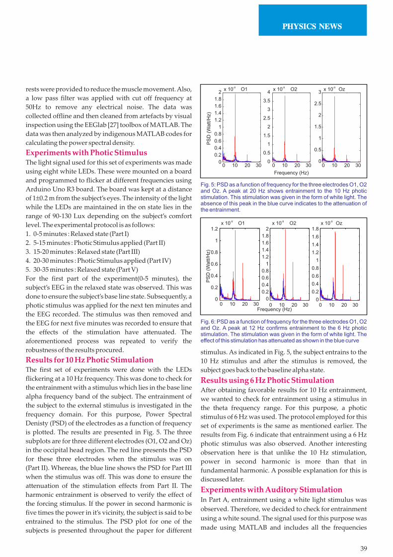
Results using 6 Hz Photic StimulationAfter obtaining favorable results for 10 Hz entrainment,

we wanted to check for entrainment using a stimulus in

the theta frequency range. For this purpose, a photic

stimulus of 6 Hz was used. The protocol employed for this

set of experiments is the same as mentioned earlier. The

results from Fig. 6 indicate that entrainment using a 6 Hz

photic stimulus was also observed. Another interesting

observation here is that unlike the 10 Hz stimulation,

power in second harmonic is more than that in

fundamental harmonic. A possible explanation for this is

discussed later.

Experiments with Auditory StimulationIn Part A, entrainment using a white light stimulus was

observed. Therefore, we decided to check for entrainment

using a white sound. The signal used for this purpose was

made using MATLAB and includes all the frequencies

39

Fig. 5: PSD as a function of frequency for the three electrodes O1, O2 and Oz. A peak at 20 Hz shows entrainment to the 10 Hz photic stimulation. This stimulation was given in the form of white light. The absence of this peak in the blue curve indicates to the attenuation of the entrainment.

3

2.5

2

1.5

1

0.5

0

2

1.8

1.6

1.4

1.2

1

0.8

0.6

0.4

0.2

0

4

3.5

3

2.5

2

1.5

1

0.5

00 10 20 30 0 10 20 30 0 10 20 30

Frequency (Hz)

Oz-9x 10-9x 10-9x 10 O1 O2

PS

D (

Watt/H

z)

Fig. 6: PSD as a function of frequency for the three electrodes O1, O2 and Oz. A peak at 12 Hz confirms entrainment to the 6 Hz photic stimulation. The stimulation was given in the form of white light. The effect of this stimulation has attenuated as shown in the blue curve

2

1.8

1.6

1.4

1.2

1

0.8

0.6

0.4

0.2

0

1.8

1.6

1.4

1.2

1

0.8

0.6

0.4

0.2

0

1.2

1

0.8

0.6

0.4

0.2

0

Frequency (Hz)

Oz-9x 10-9x 10-9x 10 O1 O2

PS

D (

Watt/H

z)

0 10 20 30 0 10 20 30 0 10 20 30

from 1 to 10000 Hz distributed uniformly. The

experimental protocol was the same as that for visual

stimulus. Simultaneous EEG was recorded with sound

stimulus given for 10 minutes twice and separated by

resting periods of 5 minutes. The PSD plot for the same

subject as used for the visual stimulus is presented to get

an equitable comparison between the two stimuli

presented. The intensity of the sound stimulus was

adjusted according to the subject’s comfort level.

However, the PSD is now plotted for the electrodes T5 and

T6 in the auditory processing area.

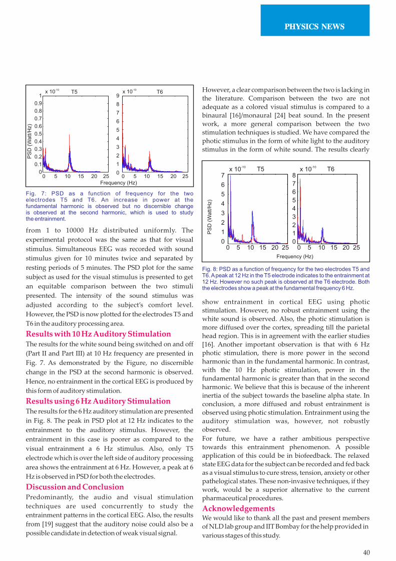
Results with 10 Hz Auditory StimulationThe results for the white sound being switched on and off

(Part II and Part III) at 10 Hz frequency are presented in

Fig. 7. As demonstrated by the Figure, no discernible

change in the PSD at the second harmonic is observed.

Hence, no entrainment in the cortical EEG is produced by

this form of auditory stimulation.

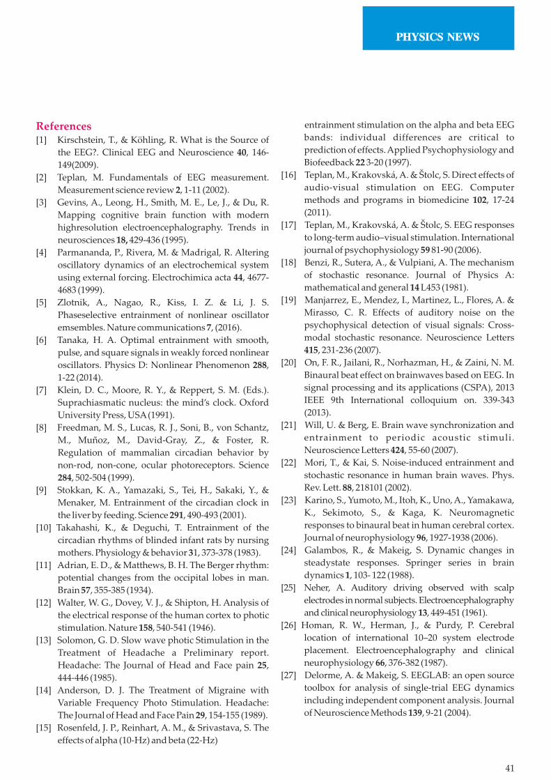
Results using 6 Hz Auditory StimulationThe results for the 6 Hz auditory stimulation are presented

in Fig. 8. The peak in PSD plot at 12 Hz indicates to the

entrainment to the auditory stimulus. However, the

entrainment in this case is poorer as compared to the

visual entrainment a 6 Hz stimulus. Also, only T5

electrode which is over the left side of auditory processing

area shows the entrainment at 6 Hz. However, a peak at 6

Hz is observed in PSD for both the electrodes.

Discussion and ConclusionPredominantly, the audio and visual stimulation

techniques are used concurrently to study the

entrainment patterns in the cortical EEG. Also, the results

from [19] suggest that the auditory noise could also be a

possible candidate in detection of weak visual signal.

However, a clear comparison between the two is lacking in

the literature. Comparison between the two are not

adequate as a colored visual stimulus is compared to a

binaura eat sound. In the present l [16]/monaural [24] b

work, a more general comparison between the two

stimulation techniques is studied. We have compared the

photic stimulus in the form of white light to the auditory

stimulus in the form of white sound. The results clearly

show entrainment in cortical EEG using photic

stimulation. However, no robust entrainment using the

white sound is observed. Also, the photic stimulation is

more diffused over the cortex, spreading till the parietal

head region. This is in agreement with the earlier studies

[16]. Another important observation is that with 6 Hz

photic stimulation, there is more power in the second

harmonic than in the fundamental harmonic. In contrast,

with the 10 Hz photic stimulation, power in the

fundamental harmonic is greater than that in the second

harmonic. We believe that this is because of the inherent

inertia of the subject towards the baseline alpha state. In

conclusion, a more diffused and robust entrainment is

observed using photic stimulation. Entrainment using the

auditory stimulation was, however, not robustly

observed.

For future, we have a rather ambitious perspective

towards this entrainment phenomenon. A possible

application of this could be in biofeedback. The relaxed

state EEG data for the subject can be recorded and fed back

as a visual stimulus to cure stress, tension, anxiety or other

pathelogical states. These non-invasive techniques, if they

work, would be a superior alternative to the current

pharmaceutical procedures.

AcknowledgementsWe would like to thank all the past and present members

of NLD lab group and IIT Bombay for the help provided in

various stages of this study.

40

Fig. 7: PSD as a function of frequency for the twoelectrodes T5 and T6. An increase in power at thefundamental harmonic is observed but no discernible changeis observed at the second harmonic, which is used to studythe entrainment.

1

0.9

0.8

0.7

0.6

0.5

0.4

0.3

0.2

0.1

0

9

8

7

6

5

4

3

2

1

0

Frequency (Hz)

PS

D (

Watt/H

z)

0 5 10 15 20 25 0 5 10 15 20 25

T6T5-10x 10-10x 10

Fig. 8: PSD as a function of frequency for the two electrodes T5 and T6. A peak at 12 Hz in the T5 electrode indicates to the entrainment at 12 Hz. However no such peak is observed at the T6 electrode. Both the electrodes show a peak at the fundamental frequency 6 Hz.

Frequency (Hz)

PS

D (

Watt/H

z)

7

6

5

4

3

2

1

0

8

7

6

5

4

3

2

1

00 5 10 15 20 25 0 5 10 15 20 25

T6T5 -10x 10

-10x 10

References[1] Kirschstein, T., & Köhling, R. What is the Source of

the EEG?. Clinical EEG and Neuroscience 40, 146-

149(2009).

[2] Teplan, M. Fundamentals of EEG measurement.

Measurement science review 2, 1-11 (2002).

[3] Gevins, A., Leong, H., Smith, M. E., Le, J., & Du, R.

Mapping cognitive brain function with modern

highresolution electroencephalography. Trends in

neurosciences 18, 429-436 (1995).

[4] Parmananda, P., Rivera, M. & Madrigal, R. Altering

oscillatory dynamics of an electrochemical system

using external forcing. Electrochimica acta 44, 4677-

4683 (1999).

[5] Zlotnik, A., Nagao, R., Kiss, I. Z. & Li, J. S.

Phaseselective entrainment of nonlinear oscillator

emsembles. Nature communications 7, (2016).

[6] Tanaka, H. A. Optimal entrainment with smooth,

pulse, and square signals in weakly forced nonlinear

oscillators. Physics D: Nonlinear Phenomenon 288,

1-22 (2014).

[7] Klein, D. C., Moore, R. Y., & Reppert, S. M. (Eds.).

Suprachiasmatic nucleus: the mind’s clock. Oxford

University Press, USA (1991).

[8] Freedman, M. S., Lucas, R. J., Soni, B., von Schantz,

M., Muñoz, M., David-Gray, Z., & Foster, R.

Regulation of mammalian circadian behavior by

non-rod, non-cone, ocular photoreceptors. Science

284, 502-504 (1999).

[9] Stokkan, K. A., Yamazaki, S., Tei, H., Sakaki, Y., &

Menaker, M. Entrainment of the circadian clock in

the liver by feeding. Science 291, 490-493 (2001).

[10] Takahashi, K., & Deguchi, T. Entrainment of the

circadian rhythms of blinded infant rats by nursing

mothers. Physiology & behavior 31, 373-378 (1983).

[11] Adrian, E. D., & Matthews, B. H. The Berger rhythm:

potential changes from the occipital lobes in man.

Brain 57, 355-385 (1934).

[12] Walter, W. G., Dovey, V. J., & Shipton, H. Analysis of

the electrical response of the human cortex to photic

stimulation. Nature 158, 540-541 (1946).

[13] Solomon, G. D. Slow wave photic Stimulation in the

Treatment of Headache a Preliminary report.

Headache: The Journal of Head and Face pain 25,

444-446 (1985).

[14] Anderson, D. J. The Treatment of Migraine with

Variable Frequency Photo Stimulation. Headache:

The Journal of Head and Face Pain 29, 154-155 (1989).

[15] Rosenfeld, J. P., Reinhart, A. M., & Srivastava, S. The

effects of alpha (10-Hz) and beta (22-Hz)

entrainment stimulation on the alpha and beta EEG

bands: individual differences are critical to

prediction of effects. Applied Psychophysiology and

Biofeedback 22 3-20 (1997).

[16] Teplan, M., Krakovská, A. & Štolc, S. Direct effects of

audio-visual stimulation on EEG. Computer

methods and programs in biomedicine 102, 17-24

(2011).

[17] Teplan, M., Krakovská, A. & Štolc, S. EEG responses

to long-term audio–visual stimulation. International

journal of psychophysiology 59 81-90 (2006).

[18] Benzi, R., Sutera, A., & Vulpiani, A. The mechanism

of stochastic resonance. Journal of Physics A:

mathematical and general 14 L453 (1981).

[19] Manjarrez, E., Mendez, I., Martinez, L., Flores, A. &

Mirasso, C. R. Effects of auditory noise on the

psychophysical detection of visual signals: Cross-

modal stochastic resonance. Neuroscience Letters

415, 231-236 (2007).

[20] On, F. R., Jailani, R., Norhazman, H., & Zaini, N. M.

Binaural beat effect on brainwaves based on EEG. In

signal processing and its applications (CSPA), 2013

IEEE 9th International colloquium on. 339-343

(2013).

[21] Will, U. & Berg, E. Brain wave synchronization and

entrainment to periodic acoustic stimuli.

Neuroscience Letters 424, 55-60 (2007).

[22] Mori, T., & Kai, S. Noise-induced entrainment and

stochastic resonance in human brain waves. Phys.

Rev. Lett. 88, 218101 (2002).

[23] Karino, S., Yumoto, M., Itoh, K., Uno, A., Yamakawa,

K., Sekimoto, S., & Kaga, K. Neuromagnetic

responses to binaural beat in human cerebral cortex.

Journal of neurophysiology 96, 1927-1938 (2006).

[24] Galambos, R., & Makeig, S. Dynamic changes in

steadystate responses. Springer series in brain

dynamics 1, 103- 122 (1988).

[25] Neher, A. Auditory driving observed with scalp

electrodes in normal subjects. Electroencephalography

and clinical neurophysiology 13, 449-451 (1961).

[26] Homan, R. W., Herman, J., & Purdy, P. Cerebral

location of international 10–20 system electrode

placement. Electroencephalography and clinical

neurophysiology 66, 376-382 (1987).

[27] Delorme, A. & Makeig, S. EEGLAB: an open source

toolbox for analysis of single-trial EEG dynamics

including independent component analysis. Journal

of Neuroscience Methods 139, 9-21 (2004).

41

Dr. Sarika Jalan is an Associate Professor in the Discipline of Physics and an adjunct faculty in Centre for Biosciences and Biomedical Engineering at Indian Institute of Technology Indore. She obtained her Ph.D. from Physical Research Laboratory, Ahmedabad in 2004 in Physics with the specialization in Nonlinear dynamics and complex systems. After post‐doctoral experience at MPI‐MiS, MPI‐PKS and NUS Singapore, she established Complex Systems Lab upon joining IIT Indore as Assistant Professor in December 2010. Dr. Jalan has authored over 60 publications in peer‐reviewed journals. She has made fundamental contributions in nonlinear dynamics research through her discoveries of novel collective states and complex dynamical behavior of coupled networks. She has played a key role in applying spectral graph and random matrix theories to complex systems research that has provided valuable insights into hidden structural symmetries of networks. An outstanding feature of her research is demonstration of practical applications of network science in a wide range of potential problems ranging from early cancer detection to optimized synchronization.Camellia Sarkar is a graduate student at Complex Systems Lab, Indian Institute of Technology Indore. After obtaining a M.Tech. degree in Biotechnology from SRM University, Chennai, she joined Complex Systems Lab in 2013. Her Ph.D. work encompasses investigations on complex biological and social systems using tools from network theory and spectral graph theory, with prime emphasis on protein‐protein interaction networks, gene regulatory networks, codon‐based co‐occurrence networks, movie co‐actor networks and scientific collaboration networks.

42

Complex networks: an introduction Networks present a simple framework to model complex systems comprising of interacting elements. Modern research on network science begun with an objective for characterizing topology of real-world systems consisting of large number of interacting units. In the past two decades, network theory has been used extensively to model real-world systems spanning from biology to physics to technology to society, offering scientists a chance to address in quantitative terms various generic features of natural systems and to understand and predict their behaviour. Networks comprise of two basic ingredients: (i) nodes (or vertices) and (ii) links (or connections). The transportation system of a country is a network of cities (nodes) connected through railways (links). The brain can be represented as a network of neurons (nodes) connected through axons (links).

Facebook is a network of people (nodes) connected

through friendships (links). Clearly, network provides a

very simplified representation of complex relationships

between objects of a system by ignoring many intricate

details of the underlying system. For instance, in case of

the neural network representation of brain, we ignore

strength of the action potential across the axons or specific

nature of neurons (excitatory or inhibitory). Similarly, for

the case of rail transportation network, the length and

width of the railway tracks (narrow gauge or broad

gauge), size of the cities connected through railways or the

frequency of trains can be ignored. One might wonder as

to how after ignoring so much crucial information,

modelling a system under network theory framework can

be of any use. Here comes the triumph of network science.

Complex Networks: an emerging branch of science Sarika Jalan and Camellia Sarkar

Complex Systems Lab, Indian Institute of Technology Indore, Simrol, Indore - 453552

Network Nodes Links

WWW Webpages URLs

Internet Routers Physical/ wireless links

E. coli metabolic Metabolites Chemical reactions

network

Citation Papers Citations

Email Email addresses Emails

Protein-protein Proteins Binding

Interactions interactions

Phone call Subscribers Calls

Word-synonym Words Synonyms

Movie-actor Actors Movies

Co-authorship Authors Publications

Food web Species Predator-prey

interactions

Words co-occurrence Words Sentence

Power grid Sub-stations High voltage lines

C. elegans neural Neurons Axons

network

Table 1: Examples of complex systems

represented by networks.

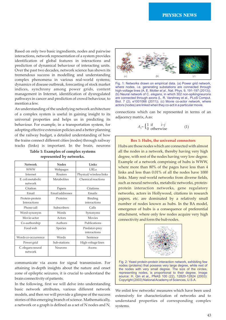
Fig. 1: Networks drawn on empirical data. (a) Power grid network, where nodes, i.e. generating substations are connected through high-voltage lines (A. E. Motter et al., Nat. Phys. 9, 191-197 (2013)). (b) Neural network of C. elegans, in which 302 non-spikingneurons are connected through axons (L. R. Varshney et al., PLoS Comput. Biol. 7 (2), e1001066 (2011)). (c) Movie co-actor network, where actors (nodes) are linked when they co-act in a particular movie.

Based on only two basic ingredients, nodes and pairwise interactions, network representation of a system provides identification of global features in interactions and prediction of dynamical behaviour of interacting units. Over the past two decades, network science has shown its tremendous success in modelling and understanding complex phenomena in various real-world systems; dynamics of disease outbreak, forecasting of stock market indices, synchrony among power grids, content management in Internet, identification of dysregulated pathways in cancer and prediction of crowd behaviour, to mention a few.

An understanding of the underlying network architecture

of a complex system is useful in gaining insight to its

universal properties and helps us in predicting its

behaviour. For example, in a transportation system, for

adopting effective extension policies and a better planning

of the railway budget, a detailed understanding of how

the trains connect different cities (nodes) through railway

tracks (links) is important. In the brain, neurons

communicate via axons for signal transmission. For

attaining in-depth insights about the nature and onset

zone of epileptic seizures, it is crucial to understand the

brain connectivity of patients.

In the following, first we will delve into understanding

basic network attributes, various different network

models, and then we will provide a glimpse of the success

stories of this emerging branch of science. Mathematically,

a network or a graph is defined as a set of N nodes and Nc

connections which can be represented in terms of an

adjacency matrix, A as:

We enlist few networks' measures which have been used

extensively for characterization of networks and to

understand properties of corresponding complex

systems.

43

10

ifotherwise

Ii~jA = { (1)ij

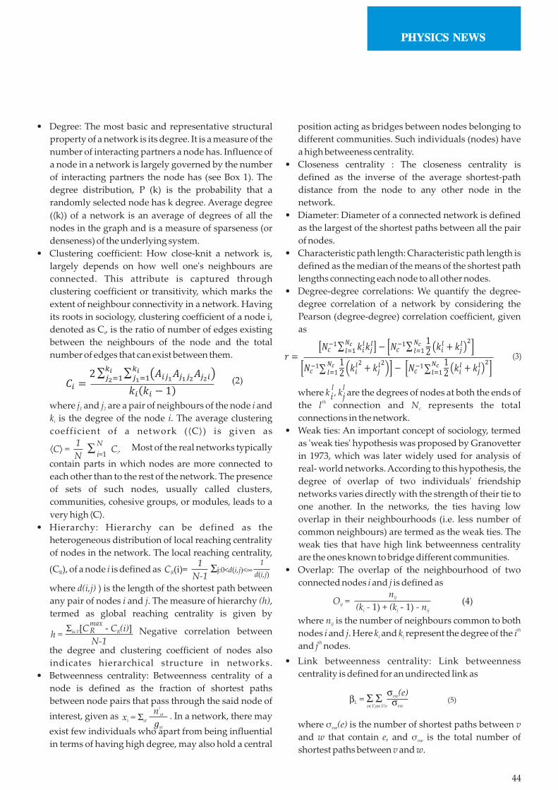
Box 1: Hubs, the universal connectors

Hubs are those nodes which are connected with almost

all the nodes in a network, thereby having very high

degree, with rest of the nodes having very low degree.

Example of a network comprising of hubs is WWW,

where more than 80% of the pages have less than 4

links and less than 0.01% of all the nodes have 1000

links. Many real-world networks from diverse fields,

such as neural networks, metabolic networks, protein-

protein interaction networks, gene regulatory

networks, actors in Hollywood, citations in research

papers, etc. are dominated by a relatively small

number of nodes known as hubs. In the BA model,

emergence of hubs is a consequence of preferential

attachment, where only few nodes acquire very high

connectivity and form the hub nodes.

Fig. 2: Yeast protein-protein interaction network, exhibiting few nodes (proteins) that possess very large degree, while rest of the nodes with very small degree. The size of the circles, representing nodes, is proportional to their degree. Image source: H. Qin et al., PNAS 100 (22), 12820-12824 (2003): Copyright (2003) National Academy of Sciences, U.S.A.

position acting as bridges between nodes belonging to

different communities. Such individuals (nodes) have

a high betweeness centrality.

• Closeness centrality : The closeness centrality is

defined as the inverse of the average shortest-path

distance from the node to any other node in the

network.

• Diameter: Diameter of a connected network is defined

as the largest of the shortest paths between all the pair

of nodes.

• Characteristic path length: Characteristic path length is

defined as the median of the means of the shortest path

lengths connecting each node to all other nodes.

• Degree-degree correlations: We quantify the degree-

degree correlation of a network by considering the

Pearson (degree-degree) correlation coefficient, given

as

where k , k are the degrees of nodes at both the ends of ththe l connection and N represents the total c

connections in the network.

• Weak ties: An important concept of sociology, termed

as 'weak ties' hypothesis was proposed by Granovetter

in 1973, which was later widely used for analysis of

real- world networks. According to this hypothesis, the

degree of overlap of two individuals' friendship

networks varies directly with the strength of their tie to

one another. In the networks, the ties having low

overlap in their neighbourhoods (i.e. less number of

common neighbours) are termed as the weak ties. The

weak ties that have high link betweenness centrality

are the ones known to bridge different communities.

• Overlap: The overlap of the neighbourhood of two

connected nodes i and j is defined as

where n is the number of neighbours common to both ij

thnodes i and j. Here k and k represent the degree of the i i j

thand j nodes.

• Link betweenness centrality: Link betweenness

centrality is defined for an undirected link as

where σ (e) is the number of shortest paths between v vw

and w that contain e, and σ is the total number of vw

shortest paths between v and w.

• Degree: The most basic and representative structural

property of a network is its degree. It is a measure of the

number of interacting partners a node has. Influence of

a node in a network is largely governed by the number

of interacting partners the node has (see Box 1). The

degree distribution, P (k) is the probability that a

randomly selected node has k degree. Average degree

(⟨k⟩) of a network is an average of degrees of all the

nodes in the graph and is a measure of sparseness (or

denseness) of the underlying system.

• Clustering coefficient: How close-knit a network is,

largely depends on how well one's neighbours are

connected. This attribute is captured through

clustering coefficient or transitivity, which marks the

extent of neighbour connectivity in a network. Having

its roots in sociology, clustering coefficient of a node i,

denoted as C , is the ratio of number of edges existing i

between the neighbours of the node and the total

number of edges that can exist between them.

where j and j are a pair of neighbours of the node i and 1 2

k is the degree of the node i. The average clustering i

coefficient of a network (⟨C⟩) is given as

Most of the real networks typically

contain parts in which nodes are more connected to

each other than to the rest of the network. The presence

of sets of such nodes, usually called clusters,

communities, cohesive groups, or modules, leads to a

very high ⟨C⟩.

• Hierarchy: Hierarchy can be defined as the

heterogeneous distribution of local reaching centrality

of nodes in the network. The local reaching centrality,

(C ), of a node i is defined as R

where d(i,j) ) is the length of the shortest path between

any pair of nodes i and j. The measure of hierarchy (h),

termed as global reaching centrality is given by

Negative correlation between

the degree and clustering coefficient of nodes also

indicates hierarchical structure in networks.

• Betweenness centrality: Betweenness centrality of a

node is defined as the fraction of shortest paths

between node pairs that pass through the said node of

interest, given as . In a network, there may

exist few individuals who apart from being influential

in terms of having high degree, may also hold a central

b = S SL vÎV wÎV/vs

(5)svw

s (e)vw

nij

(k - 1) + (k - 1) - ni j ij

O = ij (4)

in st

gst

x = Si st

S [C - C (i)]iÎV R

N-1h =

maxR

1

N-1Sj:0<d(i,j)<¥

1

d(i,j)C (i)=R

1

NåáCñ =

N

i=1C .i

44

l

jl

/ /(2)

(3)/

/ /

/

Note that here we have restricted ourselves to define

widely used structural measures in network science. With

the growing success of network science over the years,

several other concepts and measures have been coined

and realized, which effectively capture many intrinsic

behaviours as well as characterize complexity of

underlying complex systems [5].

Different network models

Historically, the study of networks has resided within a

domain of discrete mathematics known as graph theory.

Since its birth in 1736, when the Swiss mathematician

Leonhard Euler published the solution to the Königsberg

bridge problem, graph theory has witnessed many

exciting developments and has provided solutions

to various intricate problems. Apart from the

developments in the field of mathematical graph theory,

analysis of social networks started gaining prominence

around 1920s, with emphasis on understanding

relationships between the individuals in a society,

economic transactions or trade among nations. Until the

1950s, networks were realized under the graph theory

framework as regular graphs. During the late 1950's it was

contemplated that large-scale graphs with no apparent

design principles can be categorized as 'random graphs',

which eventually turned out to be the simplest and

straightforward representation of a complex system. The

most popular model for random networks was proposed

by pioneering mathematicians, Paul Erdös and Alfred

Rényi in 1959.

45

Box 2 : Importance of nodes having high betweenness centrality

As defined betweenness centrality of a node provides insight to importance of a node based on its existence on the

shortest paths connecting different pairs of the nodes. Connectivity of the nodes scales positively with the

betweenness centrality. However, there may exist nodes which despite having low degree, have high betweenness

centrality. Such types of nodes are found to occur in networks where groups of nodes termed as modules,

communities or subgraphs exist, where they act as bridges between different groups. Such nodes are found to be

functionally important as well. For instance, it is shown in empirical investigations carried out on metabolic

networks of 12 different organisms by Guimera and Amaral, where metabolites are nodes and reactions are the

links, that there exist few nodes in the network which have low connectivity yet high betweenness centrality (Fig.

3(a)). Such metabolites participating in few reactions but connecting different functional groups are found to be

more conserved as compared to other metabolites. Fig. 3(b) depicts a plot of degree of movie actors as a function of

their betweenness centrality, where the actors with low connectivity yet high betweenness centrality have an

advantage of a long span in the film industry. Another example where such nodes are prominent is the friendship

network of 34 members of a karate club at a US university, who split among two groups (blue and red coloured

nodes) following a dispute Fig. 3(c). The few connecting links between these two groups are the nodes with low

degree but high betweenness centrality. This important revelation on the structural significance of nodes guiding

their functionality and conservation, has paved way for analysis of a series of networks, such as movie co-actor

networks, protein-protein interaction networks of cancer, gene regulatory networks, for identification of nodes

having crucial importance in the system's functioning.

Fig. 3: Nodes with low degree but high betweenness centrality depicted in (a) metabolic networks (R. Guimera and L. A. N. Amaral, Nature 433 (7028), 895 (2005)), (b) movie co-actor networks (S. Jalan et al., PloS one 9 (2), e88249 (2014)) and (c) Zachary karate club network (M. E. J. Newman, PNAS 103 (23), 8577-8582 (2006): Copyright (2006) National Academy of Sciences, U.S.A.).

Erdös – Rényi model: According to this model, starting with

N nodes, every pair of nodes are connected with a

probability p, creating a graph with approximately

pN(N − 1)/2 edges distributed randomly. The majority of

nodes in this graph have their degree close to the average

degree ⟨k⟩ of the network, given as ⟨k⟩ = p(N − 1) � pN. The

degree distribution (P(k)) of a random graph was shown to

follow a binomial distribution

which for large N can be replaced with Poisson −ákñdistribution P(k) ~ e . At a very low connection

probability p, nodes are scattered in small groups

disconnected with each other. With an increase in p, there

lies a critical point around ⟨k⟩ = 1 when a connected

component starts to form (Fig. 4(c)), which by further

increase in p turns into a single giant component spanning

almost all the nodes. This model has guided our

understanding about complex networks for decades and

many real-world systems as complex and as diverse as the

cellular network and the Internet were modelled as

random graphs.

While the formulation of the random graph theory

intrigued scientists from diverse fields to venture in to

complex systems research, it also prompted

reconsideration of the notion that underlying interactions

in systems as diverse as the cell, society or the Internet are

fundamentally random. That is, could systems such as the

cell or a society function seamlessly if their molecules or

people were wired randomly together? With the growing

availability of large-scale databases and advancement in

computational facilities, a series of investigations took

place during the late 1990's on several real-world systems,

such as WWW, Internet, protein-protein interactions,

actor collaboration, neural network of C. elegans, citation

patterns in science, and so on. These investigations led to

one of the most striking discoveries in the field of complex

networks that interactions of real-world networks are “not

random” and follow some universal features.

Barabási-Albert (BA) model: Discovery of the scale-free

property of networks by Hungarian mathematicians,

Alfred László Barabási and Réka Albert in 1999 [3] marked

the rebirth of network science. They proposed that real

networks are not random as the degree distribution of

real-world networks deviate significantly from the

Poisson distribution. Using data from the World Wide

Web, which was incidently one of the largest networks 12ever built (N � 10 ) with nodes as documents that are

linked through uniform resource locators (URLs), it was

found that the degree distribution (P(k)) followed a power

law given as-gP(k)~k , (7)

where γ is the power law exponent. This intrigued an

avalanche of research leading to the discovery that many

real-world networks, spanning from protein-protein

interactions to social networks and from the citation

patterns to the interconnected hardware behind the

Internet, have a similar power law degree distribution,

independent of the nature of the system or the identity of

its constituents, making these networks radically different

from the regular lattices and the random graphs. Such

networks were termed as scale-free networks. For a wide

range of real-world networks exhibiting power law

behaviour, the power law exponent is shown to lie

between 2 and 3 (2 < γ � 3).

Several algorithms were proposed to provide an

understanding to the existence of the scale-free topology

prevalently observed in an array of real-world networks.

The most cited algorithm that explained the emergence of

scale-free behaviour was the Barabási-Albert (BA) growth

model based on preferential attachment, popularly

known as 'rich-gets-richer' model. In the BA model,

starting with a small number of nodes (say m ), in each 0

time step a new node is added with m connections. This

newly added node preferentially connects with an already

existing high degree node i with probability

After t time steps, this method results in a network

N = t + m nodes and mt edges. Such type of networks 0

characteristically have few very high degree nodes known

.

46

Fig. 4: (a) Number of nodes in the giant component (normalized) in the Erdös-Rényi random network plotted as a function of average

network connectivity. (b) Subcritical regime, where 0 < ⟨k⟩ < 1 and only few tiny clusters are present. Phase transition at the critical

point, i.e. ⟨k⟩ = 1, marking the onset of emergence of a giant

component. (d) Supercritical regime, where ⟨k⟩ > 1 and a larger fraction of nodes belong to the giant component. (e) The connected

regime with ⟨k⟩ > lnN, in which the giant component spans almost all

nodes (N ⋍ N). Image source: A.-L. Barabási, Network Science G

(Cambridge University Press, 2016).

p (k ) = (8)i

ki

S kj j

(6)

47

as hubs along with a large number of low degree nodes

(Box 1).

The results based on empirical analysis offered the

evidence that large networks self-organize into a universal

scale-invariant nature. By scale-invariant nature, one

means that scale-free networks do not have a meaningful

internal scale owing to the fact that nodes with widely

different degrees coexist in the same network. This feature

distinguishes scale-free networks from lattices, in which

all nodes have exactly the same degree, or from random

networks, whose degrees vary in a narrow range (k = ⟨k⟩ ± 1/2⟨k⟩ ). The past two decades have witnessed tremendous

amount of work on networks bearing scale-free topology

leading to several interesting revelations. One such

revelation is the robustness of scale-free networks against

random node failures. A random network undergoes an

inverse percolation transition when a critical fraction of its

nodes is randomly removed, whereas it has been shown

that scale-free networks encounter a finite size effect in

such situations, thus making scale-free networks tolerant

against random node removal or failure. Nevertheless,

due to the presence of hubs, the scale-free networks

become highly vulnerable to targeted attacks. Scale-free

networks later turned out to be very useful for

understanding and predicting behaviours of a variety of

complex systems. For example, on a scale-free network,

the epidemic threshold converges to zero which means

that even weakly virulent viruses can spread unopposed.

This is found to be true for most of the spreading

processes, from AIDS to computer viruses, where

underlying interaction networks are scale-free.

Watts-Strogatz small-world networks: Another most famous

network model is the small-world model proposed by D. J.

Watts and S. H. Strogatz in 1998 [2]. The model was

inspired from the experiment of the social psychologist

Milgram, who demonstrated that most of the people in the

United States of America have six degrees of separation

between them. In Watts-Strogatz model, starting from a

ring lattice with N nodes and ⟨k⟩ edges per vertex, each

edge is rewired at random with a probability p (0 < p < 1). r r

For p → 0, the characteristic path length of the network is L r

~ N/2⟨k⟩ >> 1. The average clustering coefficient of the

regular lattice is C~3/4. With an increase in p from p = 0, r r

there is a rapid drop in the characteristic path length while

the average clustering coefficient still remains as high as

that for the initial ring lattice. At the small-world

transition, the values of L become close to that of the

corresponding random network. Watts-Strogatz

demonstrated that many real-world networks possess

small-world behaviour marked by an existence of very

high clustering coefficient, much higher than the

corresponding random networks along with

characteristic path length being close to the corresponding

random network. This indicates that in real-world

networks, neighbours have high tendency to connect with

themselves. The neural network of Caenorhabditis elegans,

the power grid of the western United States, and the

collaboration network of film actors are few well known

examples of small-world networks. In last two decades,

several other new network models and improvised

versions of existing models have been proposed. One of

them is the much-studied variant of the Watts- Strogatz

model, proposed by Newman and Watts in 1999, in which

edges are added between randomly chosen pairs of sites,

but no edges are removed from the regular lattice.

010

-110

-210

-310

-410

-510

-610

-710

-810

-910

a.

pk

b.

Pk

010

-110

-210

-310

-410

-510

0 10

010

-110

-210

-310

-410

-510

-610

-710

-810

-910

010

-110

-210

-310

-410

-510

-610

-710

-810

-910

0 10

110

210

410

k . kin out

310

c.

0 10

110

210

410

310

k . kin out

pkpk

110

210

310k 0

101

10 2

10 kd.

k in

kout

k in

kout

Fig. 5: The degree distribution of (a) Internet, (b) protein-protein interaction, (c) email and (d) citation networks, plotted on a doubly logarithmic scale exhibits power law behaviour. Image source: A.-L. Barabási, Network Science (Cambridge University Press, 2016).

Fig. 6: (a) Schematic representation of regular, small-world and random networks, depicting random rewiring procedure. (b) Characteristic path length (L(p)) and clustering coefficent (C(p)) plotted as a function of rewiring probability (p), illustrating onset of small- world phenomenon. Image source: D. J. Watts and S. H. Strogatz, Nature 393, 440-442 (1998).

Application of network science in diverse

fields Through investigations on structural properties of various

natural and man-made complex systems, network science

has manifested remarkable success in providing

understanding to various emerging phenomena in

diverse domains of science. In the following, we will

discuss few of the breakthrough achievements of network

science, both with respect to structural properties of

networks and dynamical evolution of interacting units on

networks.

Biological systems: The most fundamental unit of all living

organisms is the cell. In each cell, there are thousands of

different molecules which coordinate with each other in

distinct fashion for carrying out various processes.

Aberrations in the activities of these agents affect cellular

processes leading to disease conditions. With the advent of

high-throughput technologies, more and more structural

and functional information about the cellular molecules,

such as genes, proteins and metabolites are being made

available with the expectation that it would lead to

consequent potential applications, for instance targeted

drug development. However, despite tremendous

research on identification and characterization of potential

regulatory genes, biomarker proteins or drug targets, yet

the way for effectively suppressing the uncontrolled

growth of cancer cells or combatting insulin resistance in

Diabetes patients, is missing at the genetic level. Network

science provides an alternate framework to disease

research which not only considers the function of

individual cellular components, but also how these

components are interconnected through a complex web of

interactions leading to the functioning of a living cell.

Protein-protein interaction (PPI) networks of various

model organisms, such as S. cerevisiae, E. coli, H. pylori, C.

elegans, D. melanogaster, etc. as well that of humans have

been extensively investigated over these years revealing

that these PPI networks have a scale-free topology in

which a few high degree proteins play a central role in

mediating interactions among numerous, less connected

proteins. This inhomogeneity in degree distribution

renders these networks tolerant to random attacks and

vulnerable to targeted attacks, emphasizing on the

importance of hub nodes both in terms of structure and

function. The analysis of protein-protein interactions has

not only helped in pinpointing specific interactions

among different proteins which are instrumental in

distinct biological processes or implicating in a disease

condition, but has also provided insight into development

or disease mechanisms at a systems level.

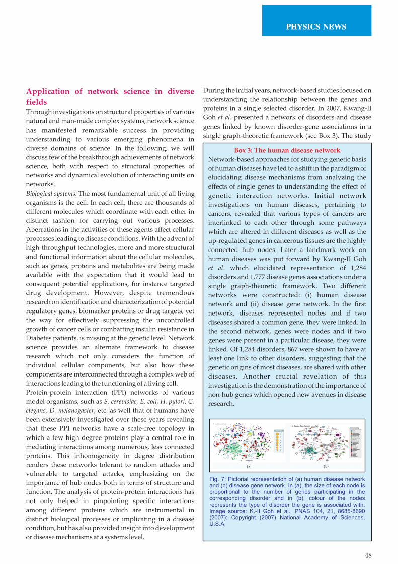
During the initial years, network-based studies focused on

understanding the relationship between the genes and

proteins in a single selected disorder. In 2007, Kwang-II

Goh et al. presented a network of disorders and disease

genes linked by known disorder-gene associations in a

single graph-theoretic framework (see Box 3). The study

48

Box 3: The human disease network

Network-based approaches for studying genetic basis

of human diseases have led to a shift in the paradigm of

elucidating disease mechanisms from analyzing the

effects of single genes to understanding the effect of

genetic interaction networks. Initial network

investigations on human diseases, pertaining to

cancers, revealed that various types of cancers are

interlinked to each other through some pathways

which are altered in different diseases as well as the

up-regulated genes in cancerous tissues are the highly

connected hub nodes. Later a landmark work on

human diseases was put forward by Kwang-II Goh

et al. which elucidated representation of 1,284

disorders and 1,777 disease genes associations under a

single graph-theoretic framework. Two different

networks were constructed: (i) human disease

network and (ii) disease gene network. In the first

network, diseases represented nodes and if two

diseases shared a common gene, they were linked. In

the second network, genes were nodes and if two

genes were present in a particular disease, they were

linked. Of 1,284 disorders, 867 were shown to have at

least one link to other disorders, suggesting that the

genetic origins of most diseases, are shared with other

diseases. Another crucial revelation of this

investigation is the demonstration of the importance of

non-hub genes which opened new avenues in disease

research.

Fig. 7: Pictorial representation of (a) human disease network and (b) disease gene network. In (a), the size of each node is proportional to the number of genes participating in the corresponding disorder and in (b), colour of the nodes represents the type of disorder the gene is associated with. Image source: K.-II Goh et al., PNAS 104, 21, 8685-8690 (2007): Copyright (2007) National Academy of Sciences, U.S.A.

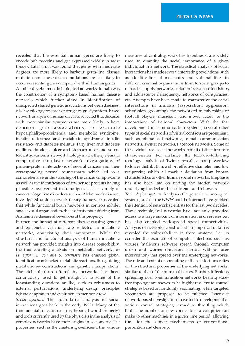
revealed that the essential human genes are likely to

encode hub proteins and get expressed widely in most

tissues. Later on, it was found that genes with moderate

degrees are more likely to harbour germ-line disease

mutations and these disease mutations are less likely to

occur in essential genes compared with all human genes.

Another development in biological networks domain was

the construction of a symptom- based human disease

network, which further aided in identification of

unexpected shared genetic associations between diseases,

disease etiology research or drug design. Symptom- based

network analysis of human diseases revealed that diseases

with more similar symptoms are more likely to have

c o m m o n g e n e a s s o c i a t i o n s , f o r e x a m p l e

hypoalphalipoproteinemia and metabolic syndrome,

insulin resistance and metabolic syndrome, insulin

resistance and diabetes mellitus, fatty liver and diabetes

mellitus, duodenal ulcer and stomach ulcer and so on.

Recent advances in network biology marks the systematic

comparative multilayer network investigations of

protein-protein interactions of several cancers and their

corresponding normal counterparts, which led to a

comprehensive understanding of the cancer complexome

as well as the identification of few sensor proteins having

plausible involvement in tumorigenesis in a variety of

cancers. Cognitive disorders such as Alzheimer's disease,

investigated under network theory framework revealed

that while functional brain networks in controls exhibit

small-world organization, those of patients suffering from

Alzheimer's disease showed loss of this property.

Further, the impact of different disease-causing genetic

and epigenetic variations are reflected in metabolic

networks, enunciating their importance. While the

structural and functional analysis of human metabolic

network has provided insights into disease comorbidity,

the flux coupling analysis on metabolic networks of

H. pylori, E. coli and S. cerevisiae has enabled global

identification of blocked metabolic reactions, thus guiding

metabolic re- constructions and genetic manipulations.

The rich platform offered by networks has been

continuously used to get insight in to some of the

longstanding questions on life, such as robustness to

external perturbations, underlying design principles

behind adaptation and evolution, to mention a few.

Social systems: The quantitative analysis of social

interactions goes back to the early 1920s. Many of the

fundamental concepts (such as the small-world property)

and tools currently used by the physicists in the analysis of

complex networks have their origins in sociometry. The

properties, such as the clustering coefficient, the various

measures of centrality, weak ties hypothesis, are widely

used to quantify the social importance of a given

individual in a network. The statistical analysis of social

interactions has made several interesting revelations, such

as identification of mechanics and vulnerabilities in

different criminal organizations from terrorist groups to

narcotics supply networks, relation between friendships

and adolescence delinquency, networks of conspiracies,

etc. Attempts have been made to characterize the social

interactions in animals (association, aggression,

submission, grooming), the networked memberships of

football players, musicians, and movie actors, or the

interactions of fictional characters. With the fast

development in communication systems, several other

types of social networks of virtual contacts are prominent,

such as phone call networks, e-mail communication

networks, Twitter networks, Facebook networks. Some of

these virtual real social networks exhibit distinct intrinsic

characteristics. For instance, the follower-following

topology analysis of Twitter reveals a non-power-law

follower distribution, a short effective diameter, and low

reciprocity, which all mark a deviation from known

characteristics of other human social networks. Emphasis

has also been laid on finding the hidden network

underlying the declared set of friends and followers.

Technological systems: Analysis of large-scale technological

systems, such as the WWW and the Internet have grabbed

the attention of network scientists for the last two decades.

These technological networks have not only provided

access to a large amount of information and services but

has also enabled widespread social connectivities.

Analysis of networks constructed on empirical data has

revealed the vulnerabilities in these systems. Let us

consider the example of computer infections such as

viruses (malicious software spread through computer

users) and worms (infections spread without user

intervention) that spread over the underlying networks.

The rate and extent of spreading of these infections relies

on the structural properties of the underlying networks,

similar to that of the human diseases. Further, infections

spreading over communication networks bearing scale-

free topology are shown to be highly resilient to control

strategies based on randomly vaccinating, while targeted

vaccination are proposed to be effective. Extensive

network-based investigations have led to development of

various control strategies, termed as throttling which

limits the number of new connections a computer can

make to other machines in a given time period, allowing

time for the slower mechanisms of conventional

prevention and clean-up.

49

q = w + s S A sin (q -q ), (9)i i ij i j

Other examples of technological networks include power

grid networks, transportation and distribution networks

and telephone networks. A power grid is a network of

gener- ating substations linked through high-voltage

transmission lines that provide long-distance transport of

electric power within and between countries. Failures on

power grids may have cascading effects, i.e. the failure of

one node may recursively provoke the failure of

connected nodes, an example being the massive blackout

in North America power grid network in 2003. Empirical

investigations suggest that the loss of a single substation

can result in substantial amount of loss (for instance, up to

25% in case of North America power grid) in transmission

efficiency by triggering an overload cascade in the

network. More importantly, it has been shown that the

connectivity loss is significantly higher on targeting high

degree or high load transmission hubs. For instance,

failure of only 4% of the nodes with high load was shown

to cause up to 60% loss of connectivity. Synchronization

and optimization-based approaches on power grid

networks were proposed to enhance their stability.

Transportation systems, along with infrastructures, such

as power grid and internet form the backbone of today's

world. Not only have they reduced the geographical gap

between people but has also encouraged trade among

nations. Investigating such systems under the network

theory framework has aided in ensuring the fastest means

of communication within the whole system. It is found

that networks of roadways, railways and airways exhibit

different topologies. The world airline network (WAN)

comprises of a small core (consisting of ~ 2.3% of the

airports) that is almost fully connected and surrounded by

a star-like periphery. Interestingly, network science

revealed that in spite of the core being so strongly

connected, removal of the core leads to more than 90% of

the airports still remaining interconnected. The impact of

load redistribution through the next shortest path in WAN

network on the profit earned from establishing the links

was demonstrated and the importance of the particular

core-periphery network structure was revealed in the

same.

Climate research: The vertices of a climate network are

identified with the spatial grid points of an underlying

global climate data set. Edges are added between pairs of

vertices depending on the degree of statistical

interdependence between the corresponding pairs of

anomaly time series taken from the climate data set. The

application of network theory to climate research has

provided interesting insights into the topology and

dynamics of the climate system over many spatial scales

ranging from local properties, such as the number of first

neighbours of a vertex to global network measures, such

as the clustering coefficient or the average path length. The

local degree centrality and related measures have been

used to identify supernodes (regions of high degree

centrality) and to associate them to known dynamical

interrelations in the atmosphere, called teleconnection

patterns. On the global scale, climate networks were found

to possess 'small-world' properties due to long-range

connections (edges linking geographically very distant

vertices), that stabilize the climate system and enhance the

energy and information transfer within it.

Dynamical systems: Investigation of emergence of

synchronization in interacting non-linear dynamical units

dates back to 1984 with the landmark works by K. Kaneko

and Y. Kuramoto, where chaotic logistic maps and

Kuramoto oscillators were investigated as interacting

units on regular networks, particularly on 1-d lattices. The

coupled oscillators model is given as

thwhere θ and ω represent phase and frequency of i i i

oscillator, respectively. σ defines the overall coupling

strength and A captures the information of network ij

architecture, which for a regular lattice case corresponds

to a banded matrix. Synchronization was one of the most

fascinating phenomena observed in non-linear dynamical

units coupled on 1-D lattice and globally coupled

networks. The remarkable advances in network science

during the late 1990's marked the rebirth of the

synchronization field. As a consequence of the

incorporation of different types of network architectures

in A , origin behind occurrence of more realistic ij

behaviour, such as c luster and hierarchical

synchronization, depicted by real-world systems were

understood. Depending upon the system's properties and

functional goal, synchronization can be desirable or

undesirable. For instance, in power grid networks, the

spontaneous synchrony among the generators of the

power grids are required to avoid massive outages. Also,

synchronization plays an important role in networks

pertaining to business, academic system, electric power

systems, digital telephony, digital audio, video,

inscription in telecommunication, flash photography etc.

and has motivated an intense research on understanding

interplay of network architecture and dynamical

evolution of units interacting through the network.

Further, with the realization of weighted network

architecture, i.e.

50

wij if i ~ j

0 otherwiseA =ij (10)

where w quantifies the strength of pair-wise interactions ij

between i and j. A great interest was born on showing how

weighted coupling configurations affect synchronization

of dynamical units. In ecological systems, the non-

uniform weight in prey-predator interactions were shown

to play a crucial role in determining the food web

dynamics.

Another extremely active research area of coupled

dynamics on networks is chimera. Analysis of chimera

states, which mark the co-existence of coherent and

incoherent states, has provided understanding to various

complex processes in nature including epileptic seizures

and unihemispheric sleep recently observed in humans,

motion of heart vessels for ventricular fibrillation and in

ecological systems. Chimera-like states have been found

to be a prominent phenomenon in modular networks, for

instance, a C. elegans neural network motivated model,

with chaotic bursting dynamics. Two-dimensional

chimera patterns have been recently reported while

studying synchronization patterns in networks of

FitzHugh-Nagumo and leaky integrate-and-fire

oscillators coupled in a two-dimensional toroidal

geometry. Game theory is another important area of

dynamical systems that has been shown to be crucially

affected by concepts of network science. Dynamical

coevolution of individual strategies along with their

interactions architecture has been explored in the context

of evolutionary game theory under the network

framework. In an investigation, by equipping individuals

with the capacity to control the number, nature, and

duration of their interactions with others, an active linking

dynamics was introduced which led to networks

exhibiting different degrees of heterogeneity.

Furthermore, problems as grave as the dynamics of

epidemic spread has also been successfully modelled and

understood under the network theory framework. Using

the so-called susceptible / infective / removed (SIR)

models, the effect of network topology on the rate and

pattern of disease spread has been investigated. It has

been shown that the growth time scale of outbreaks is

inversely proportional to the network degree fluctuations,

signalling that epidemics spread almost instantaneously

in networks with scale-free degree distributions.

Consequently, strategies to devise dynamic control

strategies in populations with heterogeneous connectivity

pattern have also been developed.

Conclusions and future scope The advent of network theory has led to an avalanche of

research accounting to around 38,00,000 research articles

published to this date. These studies have led to

fundamental understanding of critical phenomena

occurring in nature and has triggered the birth of entirely

new dimensions of research in several fields altogether.

We have learned through empirical studies, models, and

analytical approaches that real networks are far from

being random, but display generic organizing principles.

More importantly, these features are shared by a range of

complex systems. Our goal here was to summarize, in a

coherent fashion, what is known so far. Yet we believe that

the results presented here in this review are only the tip of

the iceberg. There are a lot of critical areas, such as the

fractal geometry, optimization problem, spectral graph

theory where use of network theory has led to a

reincarnation of the concepts and understanding, which

demand to be reviewed individually. In the longer run,

network theory is expected to become essential to all

branches of science as we struggle to interpret the data

pouring in from neurobiology, genomics, ecology, finance

and the World- Wide Web, to name a few.

References [1] P. Erdös and A. Rényi, Publ. Math. Inst. Hung. Acad.

Sci. 5 (1), 17-60 (1960).

[2] D. J. Watts and S. H. Strogatz, Nature 393, 440-442

(1998).

[3] A.-L. Barabási and R. Albert, Science 286 (5439), 509-

512 (1999).

[4] S. Boccaletti et al., Phys. Rep. 424 (4), 175-308 (2006).

[5] M. E. J. Newman, Networks: An Introduction,

(Oxford University Press, New York, 2010).

[6] A. Pikovsky, M. Rosenblum and J. Kurths,

Synchronization: a universal concept in nonlinear

sciences, (Cambridge University Press, New York,

2001).

51

Sumana Dutta is an Associate Professor in the Department of Chemistry, at the Indian Institute of Technology Guwahati. She pursued doctoral work at the Indian Association for the Cultivation of Science (IACS) Kolkata, where she studied the theoretical aspects of nonlinear dynamics of spatially extended systems. Later she worked at the Florida State University, USA as a Postdoctoral research associate where she started doing experiments with chemical reactions that displayed nonlinear phenomena. Her current focus of study at IIT Guwahati are the dynamics of spiral and scroll waves, and their control in both experiments and theory. Apart from teaching and research, Sumana is involved with different outreach activities and loves talking about science to the interested. She is especially passionate about popularizing science and mathematics among the school and college students.

Dhriti Mahanta completed her B.Sc (Chemistry) from Cotton College, Guwahati and M.Sc in Physical Chemistry from Gauhati University. Currently she is a PhD scholar in the Department of Chemistry, Indian Institute of Technology Guwahati (IITG). Her research interest is nonlinear dynamics of waves and patterns in excitable media.

52

Nature is the best teacher. She presents us with beautiful

views, interesting phenomena and myriad mysteries, the

understanding of which pushes the human race to new

discoveries and inventions. From the flowers in a summer

garden to snow-flakes in the winter, the rich patterns in

the coats of animals to the branching of a tree, a sense of

order lends more beauty to the eyes of the onlooker. A

close observation of such occurrences may lead one to

ponder on the cause and source of such elegance.

Nonlinearity in the Realm of ChemistrySumana Dutta and Dhriti Mahanta

Department of Chemistry, Indian Institute of Technology Guwahati, Guwahati - 781039.

Fig. 1: Patterns found in nature. (a) Flower, (b) snowflake, and (c) zebra fish.

In a more changing scenario, like the evolution and spread

of a population or the formation of galaxies, the beauty in

the crashing waves of the sea or the dunes in the desert,

there seems to be no single cord that binds these together.

These dynamical systems change with time, and yet

succeed in painting a dainty picture before us.

A brief history of dynamicsTalking of dynamics, let us make a quick review of its

study by the human race. The first systematic study of

dynamics is attributed to Sir Isaac Newton in the mid

1600's, whose three laws could determine the two-body

planetary motion. Extension of the problem to three-body

ones, required something more qualitative like the theory

put forward by Poincaré, which looked at the long term

stability of systems [1]. His theory, proposed in the late

1800's, also predicted the existence of chaos, which can be

simply defined as the high sensitivity of a system on the

initial conditions. The succeeding era discovered the

nonlinearity of several complex phenomena, which were

hard to solve by pen and paper [2]. Some relief came in the

way of computers that greatly assisted physicists to peek

into these nonlinear systems. Scientists like Lorenz used

this approach to look into the changing weather as a

convection of fluid rolls, and predict its unpredictability

[3]. This phenomenon of chaos soon found wide-scale

application in population biology. Around the same time,

Mandelbrot discovered that fractals, or self-repeating

patterns, are found in a variety of subjects, while Winfree

suggested that living beings are also a store-house of

several oscillators, like the circadian rhythms and cardiac

rhythms, following the same set of rules that govern many

other dynamical systems [4, 5].

Chemical oscillatorsToday we know that Biology is largely Chemistry, but once

they were practised as strictly different disciplines.

Oscillators were first discovered in the chemical

laboratory as heterogeneous entities, viz. an

electrochemical cell that produced oscillating current

(1828) and periodic dissolution of chromium in an acid

(1899). The first homogeneous chemical system that

demonstrated an oscillatory clockwork was the Bray

reaction [6]. This was however not well accepted in the

chemical community of the time, due to the firm belief that

any such oscillations would be against the Second Law of

thermodynamics [7]. The latter states that all spontaneous

processes will monotonically approach its final

equilibrium position. Once there, it will stay there forever,

without the influence of any external agent. So in a

universe whose entropy was ever increasing, any

organization would not be spontaneously achieved.

Evidently any such spontaneously oscillating reaction as

the above, was supposed to be like the pendulum, with the

system passing through its equilibrium state every time it

oscillated. Thus all homogeneous oscillating reactions

were deemed as impossible. The person whose discovery

was about to change all this, was the Russian scientist

Boris P. Belousov [8]. He discovered a fascinating reaction

that changed color periodically from yellow to colorless

and back. On trying to develop an inorganic analog of the

Krebs cycle, Belousov observed a mixture of bromate, 4+citric acid and ceric ions (Ce ) show the surprising

phenomenon. On further adding ferroin (a phenanthrolin

complex of iron) to the mixture, he found a striking change

in color between red and blue (Fig. 3). He tried publishing

his very carefully studied system many times from 1951 to

1958, but was repeatedly turned down by the scientific

community. Except for an unrefereed conference

proceeding, his work did not find a place in the printed

literature of that period. Later several papers were

published on this reaction, and is still being published

today. Rather, it can be said to be the best experimental tool

for chemists for the table-top study of several intriguing

nonlinear phenomena. Belousov was an unsung hero of

science in his lifetime, who was decorated with many

prizes and accolades posthumously.

53

.

Fig. 2: Dynamical patterns. (a) Sand dunes, (b) branching in trees and honeycomb, and (c) hydrodynamic patterns in cloud.

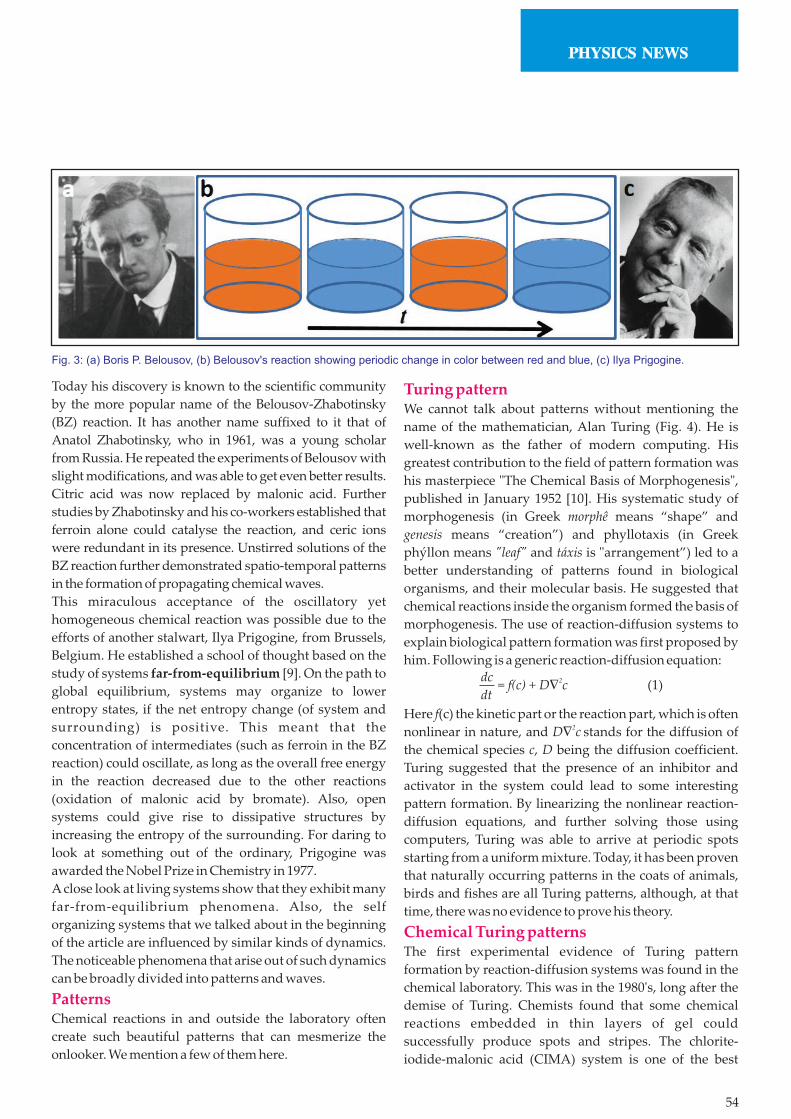
Today his discovery is known to the scientific community

by the more popular name of the Belousov-Zhabotinsky

(BZ) reaction. It has another name suffixed to it that of

Anatol Zhabotinsky, who in 1961, was a young scholar

from Russia. He repeated the experiments of Belousov with

slight modifications, and was able to get even better results.

Citric acid was now replaced by malonic acid. Further

studies by Zhabotinsky and his co-workers established that

ferroin alone could catalyse the reaction, and ceric ions

were redundant in its presence. Unstirred solutions of the

BZ reaction further demonstrated spatio-temporal patterns

in the formation of propagating chemical waves.

This miraculous acceptance of the oscillatory yet

homogeneous chemical reaction was possible due to the

efforts of another stalwart, Ilya Prigogine, from Brussels,

Belgium. He established a school of thought based on the

study of systems far-from-equilibrium [9]. On the path to

global equilibrium, systems may organize to lower

entropy states, if the net entropy change (of system and

surrounding) is positive. This meant that the

concentration of intermediates (such as ferroin in the BZ

reaction) could oscillate, as long as the overall free energy

in the reaction decreased due to the other reactions

(oxidation of malonic acid by bromate). Also, open

systems could give rise to dissipative structures by

increasing the entropy of the surrounding. For daring to

look at something out of the ordinary, Prigogine was

awarded the Nobel Prize in Chemistry in 1977.

A close look at living systems show that they exhibit many

far-from-equilibrium phenomena. Also, the self

organizing systems that we talked about in the beginning

of the article are influenced by similar kinds of dynamics.

The noticeable phenomena that arise out of such dynamics

can be broadly divided into patterns and waves.

PatternsChemical reactions in and outside the laboratory often

create such beautiful patterns that can mesmerize the

onlooker. We mention a few of them here.

Fig. 3: (a) Boris P. Belousov, (b) Belousov's reaction showing periodic change in color between red and blue, (c) Ilya Prigogine.

54

Turing patternWe cannot talk about patterns without mentioning the

name of the mathematician, Alan Turing (Fig. 4). He is

well-known as the father of modern computing. His

greatest contribution to the field of pattern formation was

his masterpiece "The Chemical Basis of Morphogenesis",

published in January 1952 [10]. His systematic study of

morphogenesis (in Greek morphê means “shape” and

genesis means “creation”) and phyllotaxis (in Greek

phýllon means "leaf" and táxis is "arrangement”) led to a

better understanding of patterns found in biological

organisms, and their molecular basis. He suggested that

chemical reactions inside the organism formed the basis of

morphogenesis. The use of reaction-diffusion systems to

explain biological pattern formation was first proposed by

him. Following is a generic reaction-diffusion equation:

Here f(c) the kinetic part or the reaction part, which is often 2 nonlinear in nature, and DÑ c stands for the diffusion of

the chemical species c, D being the diffusion coefficient.

Turing suggested that the presence of an inhibitor and

activator in the system could lead to some interesting

pattern formation. By linearizing the nonlinear reaction-

diffusion equations, and further solving those using

computers, Turing was able to arrive at periodic spots

starting from a uniform mixture. Today, it has been proven

that naturally occurring patterns in the coats of animals,

birds and fishes are all Turing patterns, although, at that

time, there was no evidence to prove his theory.

Chemical Turing patternsThe first experimental evidence of Turing pattern

formation by reaction-diffusion systems was found in the

chemical laboratory. This was in the 1980's, long after the

demise of Turing. Chemists found that some chemical

reactions embedded in thin layers of gel could

successfully produce spots and stripes. The chlorite-

iodide-malonic acid (CIMA) system is one of the best

2= f(c) + DÑ c (1)dc

dt

examples for the production of Turing patterns in both

open and closed systems [11]. The prior is achieved by a

continuously stirred tank reactor (CSTR) that was

designed around the 1980's. In most of these systems

convection is eliminated by using thin layers of gel (often,

polyvinyl alcohol). Simple reaction-diffusion model

systems were used to simulate these experiments on the

now avai lable high-speed computers which

unambiguously proved these to be true Turing patterns.

Later variants of the CIMA reaction, and some other

systems like the thiourea-iodate-sulfite (TuIS) reaction

[Fig. 4(c)] were used to demonstrate Turing patterns and

their interesting dynamics [12].

Biological patternsObservation and speculation of the biological patterns

was what led Turing to uncover the mystery behind the

formation of many beautiful patterns in nature. From the

tiniest living cells to the organization of the galaxies,

Turing pattern can be widely observed. Another

mathematician, Jim Murray extended Turing's theory to

predict that a single mechanism can generate all the

common animal coat patterns [13]. Solving reaction-

diffusion models in different kinds of boundaries

reminiscent of animal geometry, he predicted that animals

can have spotted body and striped tail, but not striped

body and spotted tail.

In the 1980's chemists were able to produce Turing

patterns in the laboratory, but it took some more decades

for biologists to experimentally prove that the stripes on

the body of animals are truly Turing patterns. This was a

seminal achievement of Shigeru Kondo and co-workers

from Japan [14]. They used the highly documented and

well understood, zebra fish for their studies. Using lasers

they tweaked the spots on the fish's skin, and allowed

morphogenesis to turn them into beautiful Turing stripes

(Fig. 5).

Fig. 4: (a) Alan Turing, (b) fish-bone-type arrangement of leaves, (c) chemical Turing pattern in the thiourea-iodate-sulfite system [12], and (d) Turing pattern on the skin of a genet.

Liesegang ringsEven before the systematic study of biological patterns by

Turing, studies of other kinds of pattern formation was thgoing on elsewhere. In the late 19 century, a German

chemist, Raphael E. Liesegang, carried out experiments

55

Zebrafish

16 dpf Adult Initial Pattern

Simulation

Stable Pattern

(3 days after ablation)

Fig. 5: Controlling Turing pattern in the skin of zebra fish. Deduced interaction network between pigment cells and simulation. Reproduced from [14] with permission.

Fig. 6: (a) Silver dichromate precipitation patterns in the laboratory [16], and (b) Liesegang rings, Bouddi National Park, Australia.

with silver nitrate solution and potassium dichromate gel,

and obtained concentric rings of precipitation patterns.

Later several other such patterns were discovered, the

entire family of which were named after him as Liesegang

rings or patterns [15, 16] (Fig. 6). These structures are not

limited to the chemical laboratory either. The rings often

seen in sedimentary rocks have been later established to be

Liesegang rings [17]. It has been surmised that the

chemical weathering of rocks leads to the formation of the

rings due to the diffusion of oxygen in subterranean water

into pore space containing soluble ferrous iron.

Chemical gardensGiant black smokers found at hydrothermal vents in the

depths of the ocean are yet another mystery, whose energy

and chemical nutrients are the source of life for several

complex ecosystems, away from the light and energy of

the sun [18, 19]. When the superheated water close to

volcanic sources, rich in salts and minerals, comes into

contact with the near-freezing brine water of the sea, the

minerals precipitate out to form insoluble tubes [Fig. 7(b)].

Some other examples of self-organizing reaction-

precipitation processes are micro-tubes in the

biomineralized shells of marine algae, precipitation tubes

in corrosion systems, soda straw stalactites in caverns [Fig.

7(a)] and brinicles found under the ice pack of the Arctic

and Antarctic oceans [20-21]. The laboratory prototype of

these tube-forming reaction precipitation systems, is the

chemical garden [Fig. 7(c,d)]. It represents a class of

reactions involving crystals of soluble metal salts placed in

aqueous solution of an anion such as silicate, aluminate,

borate, carbonate, chromate, cyanoferrate or phosphate.

Such reactions have been known since the seventeenth

century, and are most commonly carried out using silicate

solutions, hence acquiring the name of 'silica gardens'. It is

understood that when the seed crystal of a soluble metal

salt is dropped into aqueous sodium silicate solution it

begins to dissolve and gradually gets covered by a

colloidal coating of metal silicate hydrate that acts as a

semipermeable membrane. A concentrated metal salt

solution remains inside the membrane while a silicate

solution depleted of metal salt remains outside. As a result

of the difference in osmotic pressures in these two regions,

water is drawn toward the inside of the membrane leading

to the further dissolution of the metal salt. The entry of

water causes the membrane to expand under osmotic

pressure until it ruptures ejecting a jet of metal-ion

solution into the surrounding silicate solution [22].

FractalsThe term "fractal" (in Latin frāctus means "broken" or

"fractured") was first used by mathematician Benoit

Mandelbrot in 1975 to explain the concept of fractional

dimensions of geometric patterns in nature [4]. In simple

terms, fractals stand for self-similar or self-repeating

patterns. The classic examples of fractal structures are

snow-flakes and ferns (Fig. 8). In the chemical laboratory,

often such self-replicating structures are encountered by

serendipity.

FingeringFingering is yet another class of patterns involved with

fluid flow and species transport in porous media [24]. It

occurs due to contrasts in system properties such as

gravity forces, viscosities, wettability or dissolution,

giving rise to patterns that look like fingers [25].

.

56

Fig. 7: (a) Soda straw, stalactites in a natural cave, (b) hydrothermal vent at a Mid-Atlantic Ridge [19], (c) chemical (silica) gardens in a test tube, and (d) SEMs showing a field of purple SrCO -SiO vases 3 2

and stems (false color) [23].

Fig. 8: Fractals and fingers. (a) Fern, (b) precipitation patterns of silica tubes in the laboratory (artificial color) (c) satellite image of a river passing through the mountains, and (d) experimental patterns of dissolution in a plaster-water system [26].

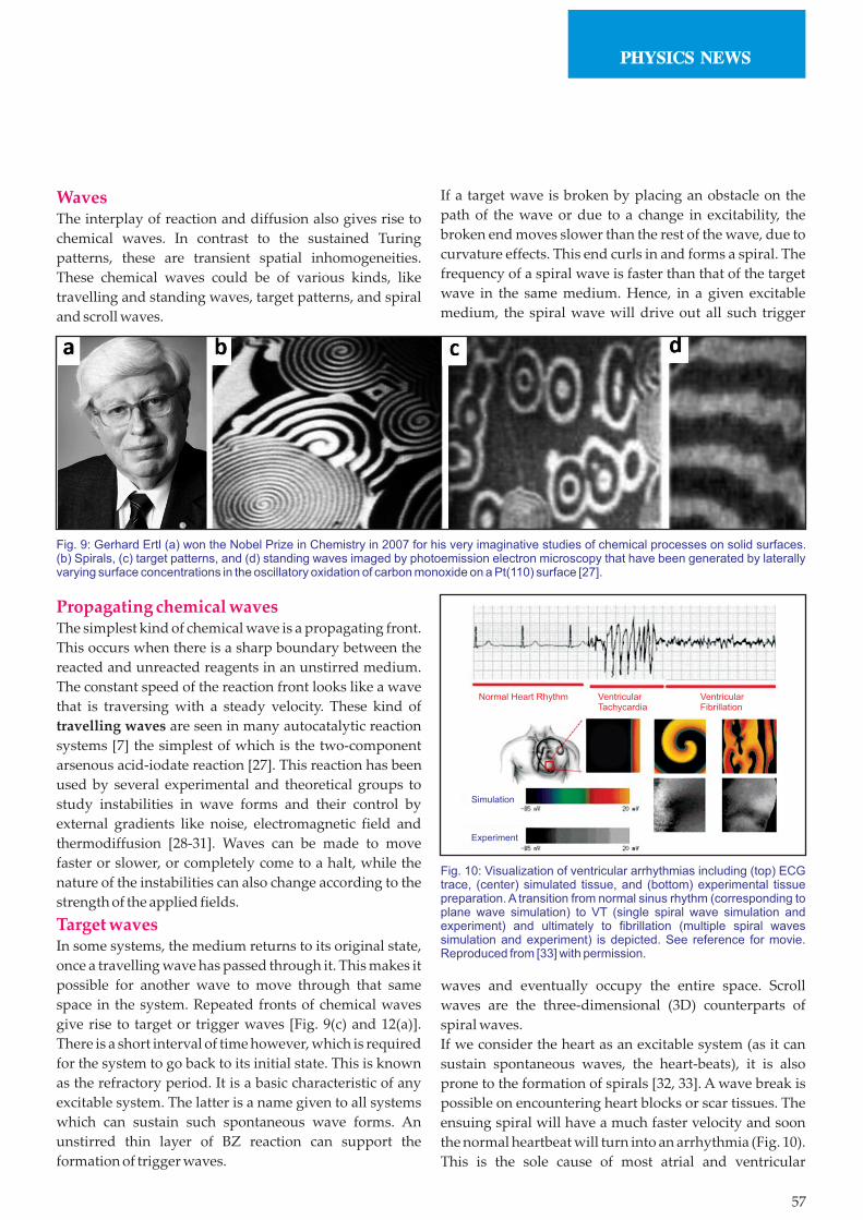
57

WavesThe interplay of reaction and diffusion also gives rise to

chemical waves. In contrast to the sustained Turing

patterns, these are transient spatial inhomogeneities.

These chemical waves could be of various kinds, like

travelling and standing waves, target patterns, and spiral

and scroll waves.

Propagating chemical waves The simplest kind of chemical wave is a propagating front.

This occurs when there is a sharp boundary between the

reacted and unreacted reagents in an unstirred medium.

The constant speed of the reaction front looks like a wave

that is traversing with a steady velocity. These kind of

travelling waves are seen in many autocatalytic reaction

systems [7] the simplest of which is the two-component

arsenous acid-iodate reaction [27]. This reaction has been

used by several experimental and theoretical groups to

study instabilities in wave forms and their control by

external gradients like noise, electromagnetic field and

thermodiffusion [28-31]. Waves can be made to move

faster or slower, or completely come to a halt, while the

nature of the instabilities can also change according to the

strength of the applied fields.

Target waves In some systems, the medium returns to its original state,

once a travelling wave has passed through it. This makes it

possible for another wave to move through that same

space in the system. Repeated fronts of chemical waves

give rise to target or trigger waves [Fig. 9(c) and 12(a)].

There is a short interval of time however, which is required

for the system to go back to its initial state. This is known

as the refractory period. It is a basic characteristic of any

excitable system. The latter is a name given to all systems

which can sustain such spontaneous wave forms. An

unstirred thin layer of BZ reaction can support the

formation of trigger waves.

If a target wave is broken by placing an obstacle on the

path of the wave or due to a change in excitability, the

broken end moves slower than the rest of the wave, due to

curvature effects. This end curls in and forms a spiral. The

frequency of a spiral wave is faster than that of the target

wave in the same medium. Hence, in a given excitable

medium, the spiral wave will drive out all such trigger

waves and eventually occupy the entire space. Scroll

waves are the three-dimensional (3D) counterparts of

spiral waves.

If we consider the heart as an excitable system (as it can

sustain spontaneous waves, the heart-beats), it is also

prone to the formation of spirals [32, 33]. A wave break is

possible on encountering heart blocks or scar tissues. The

ensuing spiral will have a much faster velocity and soon

the normal heartbeat will turn into an arrhythmia (Fig. 10).

This is the sole cause of most atrial and ventricular

Fig. 9: Gerhard Ertl (a) won the Nobel Prize in Chemistry in 2007 for his very imaginative studies of chemical processes on solid surfaces. (b) Spirals, (c) target patterns, and (d) standing waves imaged by photoemission electron microscopy that have been generated by laterally varying surface concentrations in the oscillatory oxidation of carbon monoxide on a Pt(110) surface [27].

Normal Heart Rhythm VentricularTachycardia

VentricularFibrillation

Simulation

Experiment

Fig. 10: Visualization of ventricular arrhythmias including (top) ECG trace, (center) simulated tissue, and (bottom) experimental tissue preparation. A transition from normal sinus rhythm (corresponding to plane wave simulation) to VT (single spiral wave simulation and experiment) and ultimately to fibrillation (multiple spiral waves simulation and experiment) is depicted. See reference for movie. Reproduced from [33] with permission.

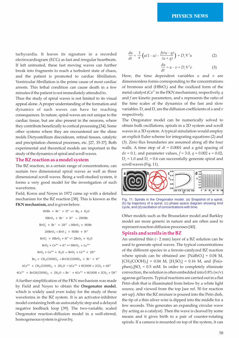
du

dt2= u - v + D v (3)v

tachycardia. It leaves its signature in a recorded

electrocardiogram (ECG) as fast and irregular heartbeats.

If left untreated, these fast moving waves can further

break into fragments to reach a turbulent state of chaos,

and the patient is promoted to cardiac fibrillation.

Ventricular fibrillation is the prime cause of most cardiac

arrests. This lethal condition can cause death in a few

minutes if the patient is not immediately attended to.

Thus the study of spiral waves is not limited to its visual

appeal alone. A proper understanding of the formation and

dynamics of such waves can have far reaching

consequences. In nature, spiral waves are not unique to the

cardiac tissue, but are also present in the neurons, where

they contribute beneficially to cortical processing [34]. Some

other systems where they are encountered are the slime

molds Dictyostellium discoideum, retinal tissues, catalytic

and precipitation chemical processes, etc. [27, 35-37]. Both

experimental and theoretical models are important in the

study of the dynamics of spiral and scroll waves.

The BZ reaction as a model systemThe BZ reaction, in a certain range of concentrations, can

sustain two dimensional spiral waves as well as three

dimensional scroll waves. Being a well-studied system, it

forms a very good model for the investigation of such

waveforms.

Field, Koros and Noyes in 1972 came up with a detailed

mechanism for the BZ reaction [38]. This is known as the

FKN mechanism, and is given below.

Here, the time dependent variables u and v are

dimensionless forms corresponding to the concentrations

of bromous acid (HBrO ) and the oxidized form of the 2

4+metal catalyst (Ce in the FKN mechanism), respectively, q

and f are kinetic parameters, and e represents the ratio of

the time scales of the dynamics of the fast and slow

variables. D and D are the diffusion coefficients of u and v u v

respectively.

The Oregonator model can be numerically solved to

obtain bulk oscillations, spirals in a 2D system and scroll

waves in a 3D system. A typical simulation would employ

an explicit Euler scheme for integrating equations (2) and

(3). Zero flux boundaries are assumed along all the four

walls. A time step of dt = 0.0001 and a grid spacing of

dx = 0.1, and parameter values, f = 3.0, q = 0.002 e = 0.02,

D = 1.0 and D = 0.6 can successfully generate spiral and u v

scroll waves (Fig. 11).

Other models such as the Brusselator model and Barkley

model are more generic in nature and are often used to

represent reaction diffusion processes [40].

Spirals and scrolls in the BZAn unstirred thin (~ 2 mm) layer of a BZ solution can be

used to generate spiral waves. The typical concentrations

of the different species in a ferroin-catalyzed BZ reaction

where spirals can be obtained are: [NaBrO ] = 0.04 M, 3

[CH (COOH) ] = 0.04 M, [H SO ] = 0.16 M, and [Fe(o-2 2 2 4

phen) ]SO = 0.5 mM. In order to completely eliminate 3 4

convection, the solution is often embedded into 0.8% (w/v)

agarose gel layers. Typical reactions are carried out in a flat

Petri-dish that is illuminated from below by a white light

source, and viewed from the top [see ref. 50 for reaction

set-up]. After the BZ mixture is poured into the Petri dish,

the tip of a thin silver wire is dipped into the middle for a

few seconds. This generates an expanding circular wave

(by acting as a catalyst). Then the wave is cleaved by some

means and it gives birth to a pair of counter-rotating

spirals. If a camera is mounted on top of the system, it can

Fig. 11: Spirals in the Oregonator model. (a) Snapshot of a spiral, (b) tip trajectory of a spiral, (c) phase space diagram showing limit cycle, and (d) oscillation of concentrations with time.

58

1e= u(1 - u) -

fv(u - q)

(u + q)2+ D u (2)u

du

dt( (

A further simplification of the FKN mechanism was made

by Field and Noyes to obtain the Oregonator model,

which is widely used even today for the study of these

waveforms in the BZ system. It is an activator-inhibitor

model containing both an autocatalytic step and a delayed

negative feedback loop [39]. The two-variable, scaled

Oregonator reaction-diffusion model in a well-stirred,

homogeneous system is given by,

be used to take pictures of the reaction. A charge coupled

device (CCD) camera, connected to a personal computer,

is usually employed for this purpose. The images thus

obtained can be later analysed to obtain dynamic data.

The dynamics of a spiral wave can be effectively described

by the motion of its tip. Initial experiments with spiral

waves revealed circular trajectories, but Winfree

suggested that spiral tips can also trace meandering

trajectories [41] (Fig. 13).

A scroll wave is a 3D entity. It can be generated at the

interface of two layers of gel. In our experiments we keep

each layer about 4 mm thick for easy visualizations. A

circular wave is generated in the middle of the first gel

layer, and when it reaches its desired size, another layer of

gel (just above its gelation temperature) is poured over it.

The semi-spherical wave from the bottom layer now

expands into the top layer, and curls in, forming a scroll

ring. The geometrical entity around which the scroll

rotates is called the filament [Fig. 12(c)]. Filaments are

thus 1D singularities in the system [42]. They either

terminate at boundaries or close in on themselves. The

filament of the scroll ring in a homogeneous system

evolves with time according to the following equation [43],

where a describes a system-specific constant line tension,

k equals the local curvature, and denotes the curve's

unit normal vector. If a > 0 (positive filament tension), the

filament will shrink and eventually disappear, which

happens in the case of our BZ system.

An interesting characteristic of this curvature-dependent

motion of scroll wave filaments is that, all nonintersecting

closed curves evolve toward a circle and all open curves

become a straight line. There are however, some special

curves, like circles, the Abresch-Langer curves, rotating

“yin-yang” patterns, and “grim reapers” or hairpins, etc.

which are shape-preserving solutions [43].

Although less frequent from the above scenario, in the

parameter region of weak excitability, negative tension of

filaments are also found. If this happens, then the scroll

rings will expand and its filament stretch and bend till it

forms a tangle of loops. Finally, filament breakage occurs

on touching the boundaries and the system may reach a

state of spatiotemporal chaos [44]. This is the predicted

mechanism of chaos and fibrillation in the cardiac tissues

however such phenomenon has not yet been observed in

the BZ system.

Control of excitation wavesIt has already been mentioned earlier that travelling waves

can be controlled by electromagnetic fields and thermal

gradients. When such fields are applied to our system

containing spiral waves, it is seen that the tip of the spiral

moves towards the area of higher excitability [Fig. 14(a)]. A

field parallel to the plane containing a scroll ring tries to

align it perpendicular to the direction of the field [45, 46].

The scroll then further traverses towards the highly

excitable end. Recent experiments have employed this

understanding to control the dynamics of scroll waves in

the BZ system [47].

Behaviour of spiral and scroll waves around

heterogeneitiesWhen spiral and scroll waves come in contact with an

unexcitable obstacle or inhomogeneity, oftentimes they

get attached to the same. This process in known as

pinning. If a circular scroll ring is pinned to two or more

Fig. 12: (a) Target wave and (b) spiral waves in the BZ system, and (c) scroll wave showing filament in blue in simulations with the Oregonator model.

N

0 10 20 30 40 50

-15

space

x

d

-10

-5

0

5

10

15

space y

Fig. 13: Spirals and scrolls in the BZ system. (a) Circular and (b) meandering trajectories of spiral tip. (c) Contraction of a scroll ring filament with time, (d) Space conserving hairpin filament [43].

59

ds

dt= ak (4)N

obstacles [Fig. 14(b, d)], its contraction can be stalled and

the lifetime of the scroll may become theoretically infinite

[48, 49]. This will be a potential threat if it occurs in the

cardiac tissues. So the understanding of the pinning

process and possible ways to unpin the scroll from its

anchors has attracted considerable attention over the past

few years. Using external gradients, scroll rings in the BZ

system, pinned to inhomogeneous obstacles were

successfully unpinned [Fig. 14(c)] [50, 51]. In the presence

of a periodic heterogeneity, a spiral tip may trace all sorts

of quantized trajectories [52].

Interaction of excitation wavesSpiral waves can interact with each other. A fast rotating

spiral can relocate a slower one, by pushing it away or

attracting it towards itself. Multiple forcing waves allows

for the capture of a spiral defect in a 2D space [53]. 3D

scroll waves on the other hand interact if they are within a

core length of each other [54]. Two scroll rings placed side-

by-side may reconnect to form a much larger scroll wave,

whose life-time will increase many-folds (Fig. 15). This can

have serious implications in biological systems. Again

scroll waves whose constituent spirals are of the same

chirality will repel each other, so much so that one of them

may touch the boundary and cause filament rupture.

The interesting properties of vortex filaments mentioned

above are not restricted to scroll rings in the BZ and

cardiac systems alone. Rather vortices in fluids, liquid

crystals and even in cosmic strings, have been seen to

interact and merge [54].

Synchronization of chemical oscillators Micro-drops of BZ oscillators, separated by oil droplets,

have been shown to synchronize with each other giving rise

to a whole school of patterns [55]. The inhibitory coupling

seen in this system is similar to what is found in interneuron

communication in the brain and coupling of semiconductor

lasers. There are several other chemical systems that show

synchronization. An example of a different genre is the

mercury beating heart system, a chemo-mechanical system

that can sustain spontaneous mechanical and

electrochemical activities, and mimics the pulsations in a

beating heart [56]. Electrical coupling of two or more such

autonomous systems show a strong synchronization in

their electro-mechanical properties (Fig. 16).

Fig. 14: (a) Spiral movement under the influence of an electric field. (b) Pinning of a circular scroll ring to (white round) glass beads. (c) Unpinning of scroll wave by the application of a thermal gradient [50]. (d) Pinning of scroll wave to a flat hexagonal mesh [49]. (All reactions performed with the BZ system.)

Fig. 15: Reconnection of scroll waves in the BZ reaction [54].

Fig. 16: Synchronization in the mercury beating heart system [56].

60

ConclusionsThis was a walk through an assortment of very visual

phenomena observed in the chemical world that has its

counterparts in many other disciplines. Understanding of

an event in a particular system aids the investigation of the

same in another. So we believe that the study of the

dynamics of pattern formation and wave nature in the

chemical systems will lead to a greater knowledge of

nonlinear systems in general. What we need to appreciate

is that the seemingly unrelated events in this universe may

have a deeper connection. There is an underlying tune that

brings forth the harmony and makes everything so

melodious.

References[1] H. Poincaré, New Methods of Celestial Mechanics, AIP-

Press, 1992.

[2] S. H. Strogatz, Nonlinear Dynamics and Chaos: with

applications to Physics, Biology, Chemistry, and

Engineering, Westview Press, 2014.

[3] E. N. Lorenz, Empirical orthogonal functions and

statistical weather prediction, Science Report 1,

Department of Meteorology, Massachusetts Institute

of Technology, 1956.

[4] B. B. Mandelbrot and P. Roberto, The Fractal Geometry

of Nature, W. H. Freeman & Co., New York, 1983.

[5] A. T. Winfree, J. Theor. Biol. 16, 15-42 (1967).

[6] W. C. Bray, J. Am. Chem. Soc. 43, 1262-1267 (1921).

[7] I. R. Epstein and J. A. Pojman, Introduction to

Nonlinear Chemical Dynamics: Oscillations, Waves,

Patterns and Chaos, Oxford University Press, New

York, 1998.

[8] A. M. Zhabotinsky, Chaos 1, 379-386 (1991).

[9] I. Prigogine, I. Stengers, and A. Toffler, Order out of

chaos: Man's new dialogue with nature, Bantam Books,

New York, 1984.

[10] A. M. Turing, Phil. Trans. R. Soc. B, 237, 37-72 (1952).

[11] R. D. Vigil, Q. Ouyang, and H. L. Swinney, Physica A

188, 17-25 (1992).

[12] J. Horváth, I. Szalai, and P. De Kepper, Science 324,

772-775 (2009).

[13] J. D. Murray, Mathematical Biology, 2nd ed., Springer-

Verlag, Berlin, 1993.

[14] A. Nakamasua, G. Takahashia, A. Kanbea, and S.

Kondo, Proc. Nat. Acad. Sci. 106, 8429–8434 (2009).

[15] K. H. Stern, Chem. Rev. 54, 79-99 (1954).

[16] I. Lagzi, Langmuir 28, 3350-3354 (2012).

[17] S. S. Augustithis and J. Ottemann, Chem. Geol. 1, 201-

209 (1966).

[18] M. J. Russell and A. J. Hall, J. Geol. Soc. 154, 377–402

(1997).

[19] D. S. Kelley, J. A. Karson, D. K. Blackman, G. L. Früh-

Green, D. A. Butterfield, M. D. Lilley, E. J. Olson, M.

O. Schrenk, K. K. Roe, G. T. Lebon, and P. Rivizzigno,

Nature 412, 145–149 (2001).

[20] S. Mann, Biomineralization: Principles and Concepts in

Bioinorganic Materials Chemistry, Oxford University

Press, Oxford, 2001.

[21] M. G. Fontana, Corrosion Engineering, 3rd ed.;

McGraw-Hill: New York, 1986.

[22] J. H. Cartwright, J. M. García-Ruiz, M. L. Novella,

and F. Otálora, J. Colloid Interface Sci. 256, 351-359

(2002).

[23] W. L. Noorduin, A. Grinthal, L. Mahadevan, and J.

Aizenberg, Science 340, 832-837 (2013).

[24] P. Ortoleva and W. Chen, Self-Organization in Far-from-

Equilibrium Reactive Porous Media Subject to Reaction

Front Fingering, in Patterns, Defects and Materials

Instabilities, edited by D. Walgraef, N. M. Ghoniem,

Kluwer Academic Publishers, London, 1990.

[25] E. Tóth-Szeles, A. Tóth, and D. Horváth, Chem.

Commun. 50, 5580-5582 (2014).

[26] G. Daccord and R. Lenormand, Nature 325, 41-43

(1987).

[27] S. Jakubith, H. H. Rotermund, W. Engel, A. von

Oertzen, and G. Ertl, Phys. Rev. Lett. 65, 3013-3016

(1990).

[28] A. Hanna, A. Saul, and K. Showalter, J. Am. Chem.

Soc. 104, 3838-3844 (1982).

[29] S. Dutta, S. S. Riaz, and D. S. Ray, Phys. Rev. E 71,

036216 (2005).

[30] S. Dutta and D. S. Ray, Phys. Rev. E 73, 026210 (2006);

S. Dutta and D. S. Ray, Phys. Rev. E 75, 016205 (2007).

[31] S. Dutta and D. S. Ray, Phys. Rev. E 75, 066206 (2007).

[32] J. Jalife, M. Delmar, J. Anumonwo, O. Berenfeld, and

J. Kalifa, Basic Cardiac Electrophysiology for the

Clinician, 2nd ed.,Wiley-Blackwell, Oxford, UK, 2009.

[33] E. M. Cherry, and F. H. Fenton, New J. Phys. 10,

125016 (2008).

[34] X. Huang, W. Xu, J. Liang, K. Takagaki, X. Gao, and J.

Y. Wu, Neuron 68, 978–990 (2010).

[35] S. C. Müller, T. Mair, and O. Steinbock, Biophys.

Chem. 72, 37-47 (1998).

[36] N. A. Gorelova and J. Bures, J. Neurobiol. 14, 353–363

(1983).

[37] A. Volford, F. Izsák, M. Ripszám, and I. Lagzi,

Langmuir 23, 961-964 (2007).

[38] R. J. Field, E. Korös, and R. M. Noyes, J. Am. Chem.

Soc. 94, 8649-8664 (1972).

[39] R. J. Field and R. M. Noyes, J. Chem. Phys. 60, 1877

(1974).

61

[40] D. Barkley, Physica D 49, 61-70 (1991).

[41] A. T. Winfree, Science 181, 937 (1973).

[42] J. P. Keener and J. J. Tyson, SIAM Rev. 34, 1-39 (1992).

[43] S. Dutta and O. Steinbock, Phys. Rev. E 81, 055202(R)

(2010).

[44] S. Alonso, F. Sagues, and A. S. Mikhailov, Science 299,

1722 (2003).

[45] M. Vinson, S. Mironov, S. Mulvey, and A. Pertsov,

Nature 386, 477-480 (1997).

[46] C. Luengviriya, S. C. Müller, and M. J. B. Hauser,

Phys. Rev. E 77, 015201 (2008).

[47] N. P. Das and S. Dutta, Phys. Rev. E 96, 022206 (2017).

[48] Z. Jiménez, B. Marts, and O. Steinbock, Phys. Rev.

Lett. 102, 244101, 1-4, 2009.

[49] D. Mahanta, S. Dutta, and O. Steinbock, Phys. Rev. E

95, 032204 (2017).

[50] N. P Das, D. Mahanta, and S. Dutta, Phys. Rev. E 90,

022916 (2014).

[51] Z. A. Jiménez, Z. Zhang, and O. Steinbock, Phys. Rev.

E 88,052918 (2013).

[52] S. Dutta and O. Steinbock, Int. J. Bif. Chaos 20, 3717-

3723 (2010).

[53] S. Dutta and O. Steinbock, Phys. Rev. E 83, 056213

(2011).

[54] N. P. Das and S. Dutta, Phys. Rev. E 91, 030901®

(2015).

[55] M. Toiya, H. O. González-Ochoa, V. K. Vanag, S.

Fraden, and I. R. Epstein, J. Phys. Chem. Lett. 1, 1241-

1246 (2010).

[56] D. K. Verma, H. Singh, A. Q. Contractor, and P.

Parmananda, J. Phys. Chem. A, 118, 4647–4651,

(2014).

62

63

News & Events

Report on the IPA DAE C. V. Raman Lecture

at Hyderabad

Prof. Bindu Bambah, School of Physics, University of

Hyderabad delivered the IPA DAE – C. V. Raman Lecture

at University of Hyderabad on the 17th of August 2017. It

was organized by the Hyderabad chapter of IPA. Prof. B.

V. R. Tata, Prof. Narayana Rao and Dr. Vudayagiri took a

keen interest to organize this event. Prof. Bambah spoke

on the topic - The Relevance of Raman Effect- from

Beverages to Black Holes.

She gave an introduction to Raman effect and followed by

a detailed account of the relevance of Raman Effect in

today's science and technology. Incidentally the lecture

was organized at Sir C. V. Raman auditorium, Science

complex, University of Hyderabad.

Report on the IPA DAE C. V. Raman Lecture

at BangaloreProf. Sriram Ramaswamy gave the IPA-DAE C. V. Raman

lecture at De Nobili Hall, St. Joseph's College on "Active

Matter and why it matters". Prof. Ramaswamy talked

about his exciting work in this field and its applications to

living materials. His presentation was attended by about

100 students and faculty who appreciated his clarity and

the presentations which brought his simulations to life.

There was an active discussion following the lecture with

questions on a broad range of topics, all of which Prof.

Ramaswamy answered diligently and with patience. The

students of St. Joseph's College were greatly benefited by

this opportunity to interact with a brilliant scientist who

was able to bring his research to an understandable level.

Prof. Ramaswamy and the local IPA Chapter very much

appreciated the effort taken by the Physics Dept. of

St. Joseph's College in facilitating this event.

64

The Institute of Physics, Bhubaneswar organized C. V.

Raman IPA-DAE Lecture under the banner of “Indian

Physics Association (IPA) - Department of Atomic Energy

(DAE) on 23rd of June, 2017 at 4.00 p.m. The lecture

entitled “The Amazing Integrable Models” was delivered

by Professor Ashok Das, University of Rochester, USA.

More than 100 scientists, researchers and students from

nearby universities, and educational institutions (Utkal

University, NISER, SOA University, OUAT and CET)

attended this lecture.

During this talk Prof. Das illustrated about integrable

models that have many unusual features. Integrable

model defines nonlinear differential/partial differential

equations that are exactly solvable. Examples include

lattice model, spin chains etc. He also described about the

integrable models in various dimension and hinted that

we do not have any 4d-integrable models. In particular, he

discussed about KdV equation, solitary wave (shallow

water wave), and nonlinear Schrödinger equation. The

KdV equation has a colourful history, which began in 1832

with John Scott Russell's celebrated pursuit on horseback

of a solitary wave along the Edinburgh- Glasgow canal. It

is the prototypical example of an exactly solvable model.

The KdV equation represents the simplest combination of

nonlinearity and dispersion in the absence of dissipation.

Owing to its nonlinearity, the KdV equation resisted

analysis for many years, and it did not come under serious

scrutiny until 1965, when Zabusky and Kruskal obtained

numerical solutions while investigating the Fermi-Pasta-

Report on IPA-DAE C. V. Raman Lecture

at Bhubaneswar

News & Events

Ulam problem of masses coupled by weakly nonlinear

springs. KdV can be solved by means of the inverse

scattering transform. The mathematical theory behind the

KdV equation is a topic of active research.

If two localized solution of KdV equation collide with each

other, remarkably after the collision they move out

maintaining their shape. These solutions which are

because of the nonlinear interactions, behave as if there

exists no interaction at all. Such solutions are called Soliton

solution. Solitons are defined as travelling wave solution

that are localized, non dispersive and those maintain their

shape even after the collision. KdV equation yielded a

startling new type of wave behavior. Soliton solutions are

now discovered for a large number of nonlinear

equations, including equations of particle physics, laser

physics, and magneto hydrodynamics.

Finally, Prof. Das mentioned that the physics related to

integrable model (KdV equation) has several connections

to physical problems and shows up in fluid dynamics,

astrophysics, biophysics, plasma, high energy and even in

defense studies. These are very special models and

describes some of the beautiful features.

P.S : The complete video lecture of Prof. A. Das on this

occasion is available in the following

link. https://www.youtube.com/watch?v=qtxpl5xEz78

65

Prof. Predhiman Krishan Kaw

(1948-2017)

OBITUARY

Prof. Predhiman Krishan Kaw, an internationally

acclaimed plasma physicist and the chief architect of

India's nuclear fusion program passed away suddenly on th18 June, 2017. A brilliant scientist who made significant

contributions to many areas of plasma physics, he was also

a wonderful teacher, a prolific researcher (with over 400

research publications), an inspiring leader and a man of

great scientific vision.

Predhiman was born in Kashmir on 15 January 1948, and

was a child prodigy who received his early schooling at

home and went on to obtain his Master's degree at the age

of 16 from the MMH College in Ghaziabad. He then joined

the Indian Institute of Technology, Delhi and was awarded

the premier Institute's first Ph.D. degree at the age of 18.

He was a student of Prof. M.S. Sodha who introduced him

to plasma physics and sparked his interest in nonlinear

phenomena. Thereafter, he joined the Princeton Plasma

Physics Laboratory for postdoctoral research. His work

during this period of 1967-71 resulted in seminal

contributions to nonlinear physics of laser - plasma

interactions and laid the foundations for much of the

current research on high power laser matter interactions.

Among his notable contributions are laser induced

parametric instabilities which lead to anomalously large

absorption as well as back and side-scattering,

filamentation of laser light due to ponderomotive forces in

a plasma and relativistic nonlinear effects which have also

found application in pulsar radiation phenomena. From

1971-75, he worked at the Physical Research Laboratory

(PRL), Ahmedabad, India, where he made important

contributions to the theory of ionospheric irregularities.

He also initiated laboratory experiments to simulate some

of the ionospheric phenomena thereby planting a seed for

future experimental plasma physics activities in India.

In 1975 Predhiman went back to Princeton and took up

research on magnetically confined fusion plasmas and

made several pioneering contributions in this area. He

showed that the decades old conventional wisdom on the

stability of drift waves in sheared geometry (a prime

candidate for transport in fusion devices) was incorrect.

He also demonstrated the existence of a coalescence

instability of magnetic islands that can be important in

diverse phenomena like disruption in tokamaks, energy

release in solar flares and sub-storm effects in tail regions

of the magnetosphere.

While still in the U.S. he noticed the remarkable and rapid

progress of tokamak research at the international level and

felt that the time was right for India to invest its intellectual

and material resources towards the development of this

future source of energy. Accordingly, he conceived and

spearheaded the effort to establish a magnetic fusion

program in India. In the late seventies and early eighties,

he and some of his colleagues at PRL succeeded in

persuading the Dept. of Science and Technology, Govt. of

India, to set up a major program of plasma physics at PRL.

He returned to India in 1982 to head this program, which

eventually evolved into the Institute for Plasma Research.

Under his leadership and guidance, the Institute made

remarkable progress on several fronts: (i) A medium sized

tokamak device called ADITYA was indigenously

designed and fabricated. This machine was commissioned

in 1989 and has led to some very novel results on

intermittency in tokamak edge turbulence. (ii) A large

number of basic experiments investigating fundamental

processes in plasmas were set up and have led to exciting

new physics. (iii) The Institute also successfully developed

a number of plasma processing technologies and some of

these technologies have been transferred to Indian

industries. (iv) The Institute carried out the

design/fabrication of an advanced steady-state

superconducting tokamak SST–1. This machine was

commissioned in 2014 and is one of the few machines of

this kind anywhere in the world. (v) The Institute

successfully spearheaded India's case for participation in

the prestigious ITER experiment and is now the nodal

domestic agency managing this participation. During the

formative years of ITER, Predhiman also played a very

important role as Chairman of the ITER STAC, the Science

and Technology Advisory Committee of ITER, by making

sure that there was no compromise in the final scientific

and technical objectives of ITER. (vi) The Institute nurtured

and trained a large number of young plasma physicists and

technical personnel through its graduate program and

technical training programs to cater to the rapidly growing

R&D activities in the field. Thus, in the span of a few years

he was successful in setting up a thriving research and

technology development program in the country and to

put India on the world map of fusion research.

ly

66

Despite his hectic schedule and commitments towards the

development of such a large research and technology

program, he never compromised on his personal research

work and continued to actively pursue it. In a pioneering

effort, he and his colleagues discovered the phenomenon

of intermittency in tokamak edge plasma turbulence of

ADITYA – a result that spawned a lot of further research in

other tokamaks of the world. At this stage Predhiman also

enlarged his research interests to more fundamental areas

like dynamics of quark-gluon plasmas, equilibria of non-

neutral electron clouds and collective effects in dusty

plasmas and other strongly coupled systems. In each of

these areas he provided new ideas, valuable insights and

in many cases strong incentives and frameworks for

laboratory experiments. He also continued his

investigations on nonlinear phenomena in relativistic

light plasma interactions and made important

contributions to the theory of envelope solitons and to the

physics of anomalous stopping of fast electrons - topics of

great interest for laser plasma based particle acceleration

schemes and the fast ignition scheme of laser fusion. He

extended activities in these frontier areas of science and

technology by forging collaborations with other active

research groups within the country and abroad. One fine

example is the establishment of collaboration between the

theory and simulation activities at IPR with TIFR

experiments in the field of laser plasma interactions. This

collaboration has led to fundamental insights in issues

pertaining to laser energy absorption, magnetic field

generation, its evolution and its turbulent characterization

in laboratory laser plasma experiments. These ideas are

tied up closely with the physics of fast ignition in laser

fusion and have also been found relevant to the

experiments on Laser Fusion in Osaka.

For his outstanding contributions and achievements,

Predhiman received many honors and awards including

the Indian National Science Academy's Young Scientists

Award in 1974, the Padma Shri award in 1985, the SS

Bhatnagar award in 1986, the IPA R.D. Birla Award in 2002

and the TWAS Prize in Physics in 2008. Most recently he

was awarded the Subrahmanyan Chandrasekhar Prize for

“outstanding contributions” in the field of plasma physics

by the Association of Asia Pacific Plasma Physics Societies.

He was a Fellow of all the major science academies in India

and also the American Physical Society.

Predhiman was a passionate scientist and a great teacher

who never tired of promoting the cause of science and

fusion. His Artsimovich Memorial Lecture delivered in

the opening session of the IAEA Fusion Energy

Conference at Wurzburg, Germany in 1992 made a lasting

impression on the international community and was a

stunning example of his remarkable perspective on the

state of international fusion research at the time and his

clear vision on the path forward. He was a great believer

and a champion of fusion research to whom the

international community frequently looked up for

guidance and inspiration. To prepare the next generation

for taking this task forward he also spent an enormous

time mentoring students and younger colleagues. He

strongly believed that science should be pursued with

complete freedom of thought and implementation. When

the IPR buildings were planned, he engaged the architects

and some of his colleagues in endless discussions to help

incorporate this concept into the design. The wide

corridors, the openness to the sky and the surroundings,

the oneness with nature and the sense of liberation that

they bring are all embodiments of this conviction.

Likewise, his office door was always open for anybody to

step in and to discuss science with him. As a human being

he was extra-ordinarily kind and gentle with infinite

patience particularly for younger colleagues. This coupled

with his infectious enthusiasm for research, his sense of

humor and informal behavior attracted many students

and scientists, not only from within the Institute but also

from the Universities and the scientific community abroad

as research collaborators. Each one of them felt enriched

and emotionally touched by his warmth and generosity of

spirit. In his more than 50 years of active scientific life,

Predhiman has not only contributed significantly to the

progress of plasma physics worldwide but has also

inspired a lot of young minds and touched a great many

human lives in an uplifting manner. He will be greatly

missed by all of them. He leaves behind an invaluable

legacy in science and humanity.

Prof. Kaw is survived by his wife Saroj and children,

Sidharth, Prashant and Puja.

Abhijit Sen

Institute for Plasma Research,

HBNI, Bhat, Gandhinagar - 382428, India

67

Prof. Yash Pal (1926-2017)

OBITUARY

Prof. Yash Pal, cosmic ray physicist, space scientist, science

communicator, and philosopher of education, passed

away on 24 July 2017 at Noida (near Delhi) at the ripe age

of 90. His coming of age coincided with India's

independence so that his life is a chronicle of a new

nation's achievements and aspirations, and towards the

end disappointment over decreasing respect for, and

interest in, science.1Early life

Yash Pal was born on 26 November1926 to Lakshmi Devi

and Ram Piyare Lal at Jhang (now in Punjab, Pakistan).

His father was employed in the ordinance department of

the defense ministry where he rose to be ordnance officer

civilian; he retired in 1958.

Yash Pal's early schooling was in Quetta in Baluchistan

where he remained till 1939. He passed the matriculation

examination in 1942 from Jabalpur, and Intermediate from

Government College Lyallpur in 1945, taking three years

instead of two because of interruption caused by illness.

Here, he met his future wife Nirmal Sharma who was an

arts student. They would marry in 1953. Yash Pal enrolled

at the prestigious Government College Lahore for B.Sc.

Honours School in Physics. In this system, the bachelor's

degree was awarded three years after Intermediate. M.Sc.

Honours School degree, by dissertation, would then be

just a year away. Yash's studies however were interrupted

by the Partition that took place on 15 August 1947.

In the meantime, early 1947, Yash Pal's father had been

transferred to Delhi, where he stayed in the Mess while his

family remained in Lahore for the sake of children's

education. He brought his family to Delhi in June 1947

which thus was spared the suffering that befell many who

came later.

Lahore was the main centre of education in Punjab. Its loss

caused institutional disruption that had to be immediately

addressed. Physics and chemistry departments were

temporarily housed in Delhi University. The arrangement

lasted from September 1947 till 30 April 1949 after which

the departments were shifted to Government College

Hoshiarpur. Yash Pal passed his B.Sc. Honours School in

Physics in 1948 and enrolled for MSc. According to family

sources, he used to travel sporadically from Delhi to

Hoshiarpur for attending classes.

Career as a ResearcherWhen still a student of M.Sc., Yash Pal was selected as a

research assistant at the recently established Tata Institute

of Fundamental Research Bombay (TIFR) with Homi

Bhabha at the helm. He formally obtained the University

degree by submitting a dissertation from Bombay.

Regrettably, but not surprisingly, neither a copy of the

dissertation not any documentation of the University's

action on it seems to have survived.

According to Yash Pal, when he joined TIFR, he went in

kurta and jeans. A very senior person told him one day that

he should not come to the institute in an informal dress as

Dr. Bhabha did not like it. He retorted: 'My letter of

appointment does not mention any dress code.' And that

was the end of the controversy. 'Dr. Bhabha never raised 2any objections thereafter.'

An event of great importance in the early TIFR's scientific

and cultural history was the arrival of Poland-born

Bernard Peters already well-known as an uncommonly

gifted cosmic ray physicist. Victim of McCarthyism in

USA, Peters first came to TIFR on a four-month visit late

1950 on behalf of the University of Rochester. He returned

to TIFR as a professor at the end of 1951 and remained here

till his departure in 1959 for Neils Bohr Institute in

Copenhagen. He remained in touch with his Indian

colleagues even after leaving India and was honoured

with the award of Padma Bhushan in 1985. Under his

stewardship, the nuclear emulsion group became very

productive and renowned. But Peters' influence on the

work culture was far more significant. Being an outsider,

he could undermine class, cultural, and linguistic

differences. He chaired the all-important meeting of the

board that interviewed candidates for selection as

research scholars. He established close relation with each

of his younger colleagues; respected individual opinions;

1Primary source of information remains Basu, Biman (2006) Yash Pal: A Life in Science (New Delhi Vigyan Prasar), based on Yash Pal's

reminiscences. I have tried to construct a connected authentic account of his early life by cross-checking with his siblings Om, Swaran and

Rajji who very kindly provided additional information.2Gauhar Raza: https://www.newslaundry.com/2017/07/26/yash-pal-obituary

1Primary source of information remains Basu, Biman (2006) Yash Pal: A Life in Science (New Delhi Vigyan Prasar), based on Yash Pal's

reminiscences. I have tried to construct a connected authentic account of his early life by cross-checking with his siblings Om, Swaran and

Rajji who very kindly provided additional information.2Gauhar Raza: https://www.newslaundry.com/2017/07/26/yash-pal-obituary

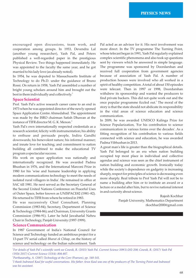
68

encouraged open discussions, team work, and

cooperation among groups. In 1953, Devendra Lal

(another young researcher), Yash Pal, and Peters

published a well-regarded paper in the prestigious

Physical Review. Two things happened immediately. He

was appointed to the faculty the same year, and he got

married to his lady love (as already noted).

In 1954, he was deputed to Massachusetts Institute of

Technology to do Ph.D. under the guidance of Bruno

Rossi. On return in 1958, Yash Pal assembled a number of

bright young scholars around him and brought out the 3best in them individually and collectively.

Space ScientistProf. Yash Pal's active research career came to an end in

1973 when he was appointed director of the newly opened

Space Application Centre Ahmedabad. The appointment

was made by the ISRO chairman Satish Dhawan at the 4instance of TIFR director M. G. K. Menon.

Yash Pal's own internationally respected credentials as a

research scientist; felicity with instrumentation; his ability

to enthuse and persuade people, Indira Gandhi

downwards; his benevolent nature; his informal manner;

and innate love for teaching; and commitment to nation

building all combined to make the educational TV

program a spectacular success.

His work on space application was nationally and

internationally recognized. He was awarded Padma

Bhushan in 1976, and the International Marconi Prize in

1980 for his 'wise and humane leadership in applying

modern communications technology to meet the needs of

isolated rural villagers in India'. He remained in office at

SAC till 1981. He next served as the Secretary General of

the Second United Nations Conference on Peaceful Uses

of Outer Space, better known as UNISPACE82 (1981–82).

He returned to TIFR from where he retired in 1983.

He was successively Chief Consultant, Planning

Commission (1983-84); Secretary, Department of Science

& Technology (1984-86); and Chairman, University Grants

Commission (1986-91). Later he held Jawaharlal Nehru

Chair in Technology, Panjab University (1997-1999).

Science CommunicationIn 1987 Government of India's National Council for

Science and Technology funded an ambitious project for a

13-part TV serial called Bharat ek Chhap, on the history of

science and technology on the Indian subcontinent. Yash

Pal acted as an advisor for it. His next involvement was

more direct. In the TV programme The Turning Point,

whose telecast began in 1991, Yash Pal regularly explained

complex scientific phenomena and also took up questions

sent by viewers which he answered in simple language.

The programme was sponsored by Doordarshan and

received full cooperation from government agencies

because of association of Yash Pal. A number of

production houses were involved who all worked in a

spirit of healthy competition. A total of about 150 episodes

were telecast. Then in 1997 or 1998, Doordarshan

withdrew its sponsorship and wanted the producers to

find private backers. This did not quite work out and the 5once popular programme fizzled out. The moral of the

story is that the state should not abdicate its responsibility

in the vital areas of science education and science

communication.

In 2009, he was awarded UNESCO Kalinga Prize for

Science Popularization, 'For his contribution to science

communication in various forms over the decades'. As a

fitting recognition of his contribution to various fields

connected with science and education, he was awarded

Padma Vibhushan in 2013.

A great man's life is greater than the biographical details.

Yash Pal belonged to an era when nation building

occupied top most place in individual and collective

agendas and science was seen as the chief instrument of

nation building and economic growth. Ironically today

while the society's dependence on gadgetry is increasing

sharply, respect for principles of science is decreasing even

more sharply. Real tribute to Prof Yash Pal will not be to

name a building after him or to institute an award or a

lecture or a medal after him, but to revive national interest

in and curiosity about science.

Rajesh Kochhar

Panjab University, Mathematics Department

rkochhar2000@gmail.com

3For details of Yash Pal's scientific work see Cowsik, R. (2015) Yash Pal. Current Science 109(1):202-208; Cowsik, R. (2017) Yash Pal

(1926-2017) Current Science 113(4): 804-807.4Parthasarathy, A. (2007) Technology at the Core (Pearson), pp. 140-141.5I thank Indraneel Kaul for useful conversations. His father Arun Kaul was one of the producers of The Turning Point and Indraneel

was his assistant.

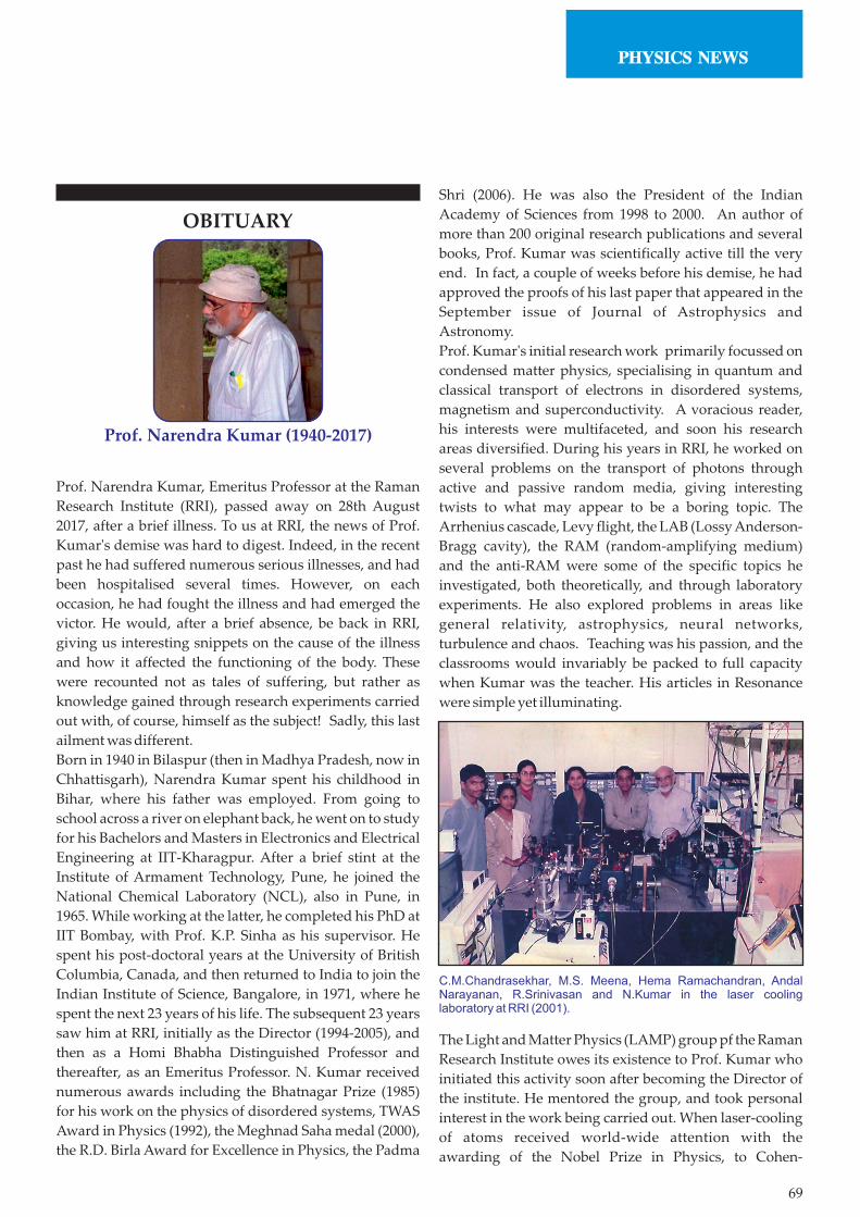
69

Prof. Narendra Kumar (1940-2017)

OBITUARY

Prof. Narendra Kumar, Emeritus Professor at the Raman

Research Institute (RRI), passed away on 28th August

2017, after a brief illness. To us at RRI, the news of Prof.

Kumar's demise was hard to digest. Indeed, in the recent

past he had suffered numerous serious illnesses, and had

been hospitalised several times. However, on each

occasion, he had fought the illness and had emerged the

victor. He would, after a brief absence, be back in RRI,

giving us interesting snippets on the cause of the illness

and how it affected the functioning of the body. These

were recounted not as tales of suffering, but rather as

knowledge gained through research experiments carried

out with, of course, himself as the subject! Sadly, this last

ailment was different.

Born in 1940 in Bilaspur (then in Madhya Pradesh, now in

Chhattisgarh), Narendra Kumar spent his childhood in

Bihar, where his father was employed. From going to

school across a river on elephant back, he went on to study

for his Bachelors and Masters in Electronics and Electrical

Engineering at IIT-Kharagpur. After a brief stint at the

Institute of Armament Technology, Pune, he joined the

National Chemical Laboratory (NCL), also in Pune, in

1965. While working at the latter, he completed his PhD at

IIT Bombay, with Prof. K.P. Sinha as his supervisor. He

spent his post-doctoral years at the University of British

Columbia, Canada, and then returned to India to join the

Indian Institute of Science, Bangalore, in 1971, where he

spent the next 23 years of his life. The subsequent 23 years

saw him at RRI, initially as the Director (1994-2005), and

then as a Homi Bhabha Distinguished Professor and

thereafter, as an Emeritus Professor. N. Kumar received

numerous awards including the Bhatnagar Prize (1985)

for his work on the physics of disordered systems, TWAS

Award in Physics (1992), the Meghnad Saha medal (2000),

the R.D. Birla Award for Excellence in Physics, the Padma

Shri (2006). He was also the President of the Indian

Academy of Sciences from 1998 to 2000. An author of

more than 200 original research publications and several

books, Prof. Kumar was scientifically active till the very

end. In fact, a couple of weeks before his demise, he had

approved the proofs of his last paper that appeared in the

September issue of Journal of Astrophysics and

Astronomy.

Prof. Kumar's initial research work primarily focussed on

condensed matter physics, specialising in quantum and

classical transport of electrons in disordered systems,

magnetism and superconductivity. A voracious reader,

his interests were multifaceted, and soon his research

areas diversified. During his years in RRI, he worked on

several problems on the transport of photons through

active and passive random media, giving interesting

twists to what may appear to be a boring topic. The

Arrhenius cascade, Levy flight, the LAB (Lossy Anderson-

Bragg cavity), the RAM (random-amplifying medium)

and the anti-RAM were some of the specific topics he

investigated, both theoretically, and through laboratory

experiments. He also explored problems in areas like

general relativity, astrophysics, neural networks,

turbulence and chaos. Teaching was his passion, and the

classrooms would invariably be packed to full capacity

when Kumar was the teacher. His articles in Resonance

were simple yet illuminating.

The Light and Matter Physics (LAMP) group pf the Raman

Research Institute owes its existence to Prof. Kumar who

initiated this activity soon after becoming the Director of

the institute. He mentored the group, and took personal

interest in the work being carried out. When laser-cooling

of atoms received world-wide attention with the

awarding of the Nobel Prize in Physics, to Cohen-

C.M.Chandrasekhar, M.S. Meena, Hema Ramachandran, Andal Narayanan, R.Srinivasan and N.Kumar in the laser cooling laboratory at RRI (2001).

70

Tannoudji, Chu and Philips in 1997, Kumar wished that

similar experiments be carried out in RRI, and thus sowed

the seeds of the cold-atoms activity in RRI. Though he was

the director of the institute, he deeply devoted to research

and his administration was minimalistic. He made it a

point to attend all talks and seminars at the institute.

“After all, we will gain in half an hour what the speaker

had to spend days (or more) reading and thinking about”,

he would say, and urge us also to take benefit of such “gain

without much pain”. Of course, Kumar did not have

much to gain, for almost always, he knew more than the

speaker, though he never let it become too obvious, even

during the question-answer sessions.

There was never a lull in the conversation when Prof.

Kumar was present – he could always find a topic to talk

on – whether it be to a child or an august personality. His

wonderful sense of humour coupled with his mastery

over English provided a combination that peppered even

everyday conversations with pun. Manuscript-writing

sessions with Kumar were very illuminating and

enjoyable. As Kumar would have put it, insomuch as the

collaborator knew English, he emerged all the more

enriched, physics-wise and English-wise, from such

endeavours.

There was more to Kumar than what has been brought out

above. He was a person of strong convictions, and did not

hesitate in stating his views and defending them, even if

they were contrary to prevailing belief. Kumar's mind was

ever active, posing interesting, non-trivial questions and

seeking answers to them, in areas ranging from physics to

cosmology to health to philosophy. Some of the questions

possessed his mind, and he would be restless till he found

the answer to them. His joy then would be immense and

child-like – a joy that he would then try to share with one

and all he met – explaining to them the problem and then

the answer. His enthusiasm was truly infectious, and

many of us have become enriched by these “Eureka

encounters” with Prof. Kumar, having now “gained

without pain”.

N. Kumar was a wonderful human-being with some

weaknesses like the inability to resist good food. He was

open to any excuse for having samosas and ice-cream –

visiting scientists, the publication of a paper, a student’s

birthday…. It is a pity that in later years his health came

in the way of such indulgence. He had a sensitive heart in

more ways than one. Any student who failed to clear a

course would be the subject of his fatherly concern - he

would take personal interest to ensure that the student

understood the subject, and performed well. A caring,

kind-hearted and generous person, he could not see others

around him suffer. Despite the numerous high posts he

held, and the many awards he received, Kumar was a

humble, down-to-earth person, and treated all as his

equal. With his passing away, we have lost a great scientist,

an inspiring teacher, and a compassionate human being.

Hema Ramachandran

Light and Matter Physics Group

Raman Research Institute

Sadashiv Nagar, Bangalore 560080.

Email : hema@rri.res.in

71

OBITUARY

On 19th April, 1975 at Kapustin Yar, the Rocket launching

site located in the then Soviet Union, a team of Indian

scientists and engineers led by a 43 year old cosmic ray

scientist U. R. Rao, was anxiously awaiting the fate of their

360 kg tetrahedron structure sitting atop a KOSMOS-3M

rocket. This was India’s maiden satellite built by Rao and

his team during the past 36 months, working tirelessly in

rather challenging conditions in an industrial shade

converted into a Space Technology facility at Peenya, near

Bangalore. The launch count down ended and the rocket

blasted off to space carrying the Indian satellite and placed

it into 570 x 610 km elliptical orbit of 50.6 degree

inclination. The satellite was christened as Aryabhata,

after the fifth century Indian mathematician and

astronomer. Aryabhata was a science mission that

included three instruments developed in Indian

laboratories for studies in X-ray Astronomy, Solar Physics

and Aeronomy. Aryabhata was followed by a succession

of remote sensing and communication satellites designed,

built and launched successfully in the following two

decades under Rao’s guidance. He was thus a true train

blazer of Indian Space Programme who played a stellar

role in developing Indian space technology capability into

world class and placed India among the front ranking

spacefaring nations.

Born on March 10, 1932 in Adamaru village of Karnataka,

Dr Udupi Ramachandra Rao obtained his M.Sc. (Physics)

degree from BHU and joined PRL, Ahmedabad as a

doctoral student under Dr Vikram Sarabhai, regarded as

the Father of Indian Space Programme. His research

involved measuring changes in the flux of μ mesons which

are secondary cosmic rays produced by interactions of

primary cosmic rays in the atmosphere. The μ mesons are

detected by recording coincidences between trays of

Geiger-Muller counters placed apart. Over the next few

years he carefully measured the diurnal variations of the

secondary cosmic rays and inferred anisotropy and

variations of galactic cosmic rays.

After obtaining his Ph. D. degree in 1960, Dr Rao joined

MIT in the USA as a post-doctoral fellow. While at MIT, he

used Mariner-2 data on solar wind velocity

measurements, in collaboration with Marcia Neugebauer

and C. W. Snyder of Jet Propulsion Laboratory, to study

the correlation between plasma velocity and propagation

of cosmic rays in the interplanetary space. Later, he moved

to the South West Centre for Advanced Studies at Dallas

(now known as the University of Texas) and flew

experiments on Space Probes Pioneer 6,7,8,9 and Explorer

34 and 41 satellites, aimed at investigating the propagation

of solar flare produced cosmic rays. In a series of seminal

papers published during 1965-1975, Rao and his co-

workers showed that solar cosmic ray protons in initial

phase show a marked anisotropy which disappears in the

decay phase due to diffusive propagation.

Rao returned to the PRL as a faculty member in 1966. At

that time, the field of X-ray astronomy which was born

with a chance discovery of the first X-ray source Sco X-1,

was a hot topic with new discoveries being reported

regularly. Rao developed a group at PRL which fabricated

instruments to be flown on rockets and balloons. With

these, they studied temporal and spectral characteristics

of cosmic ray sources and diffuse cosmic ray background.

At that time Dr Sarabhai had embarked on indigenous

development of rocket and satellite systems for India’s

nascent space programme and established the Space

Science and Technology Centre (SSTC), later named as

V i k r a m S a r a b h a i S p a c e C e n t r e ( V S S C ) a t

Thiruvananthapuram. Dr Rao was entrusted with the

responsibility of building a group that would develop

Indian satellites for science and applications. Rao created

the Satellite Systems Division (SSD) within the SSTC,

which was later relocated to Bangalore. When India and

the Soviet Union signed an agreement in 1972 to launch an

Indian built satellite by a Russian rocket, Dr Rao was

chosen as the Project Director. Dr Rao led his team from

front and instilled great self-confidence and dynamism in

his team. Successful realization and launch of Aryabhata

satellite established Rao’s credentials as an outstanding

leader who could take up technological challenges and

deliver results.

U. R. Rao (1932-2017)

72

Following the success of Aryabhata, Rao, with strong

support from Professor Satish Dhawan, Chairman of

ISRO, established ISRO SAtellite Centre (ISAC) near

National Aerospace Laboratory in Bangalore for design,

development and qualification of future Indian satellites.

In the next two decades, he and his successors developed

ISAC into an outstanding facility. Emphasis of India’s

space programme was on the development of mission that

will have a direct impact on the lives of masses. Hence,

remote sensing satellites by which natural resources could

be mapped and managed better received high priority.

The IRS series of satellites and launch of Technology

Experiment Satellite (TES) placed India as a leading nation

in remote sensing technology.

As India did not have expertise in geostationary satellites,

Dr Rao and Prof Dhawan adopted the strategy of getting

the first series of communication satellites (INSAT-1

series) built by a foreign firm, Ford Aerospace

Corporation with involvement of Indian engineers. These

engineers absorbed the technological complexities of

communication satellites which subsequently led to the

development of the next generation of such satellites, viz.

INSAT-2,3, 4 and GSAT series. Today India boasts of

capability of building communication satellites with large

number of transponders weighing about 3 tons and

covering Ka and Ku bands of frequencies.

Upon the superannuation of Prof Dhawan, Dr Rao

assumed the position of the Chairman of ISRO in 1984. He

took the decision to develop Polar Satellite Launch Vehicle

(PSLV) which would have strap-on solid boosters and a

liquid fuel second stage. Due to a technical snag the

maiden flight of PSLV was not successful. Dr Rao retired

as the Chairman ISRO in 1994. The subsequent successful

PSLV flights were primarily due to the foundation made

during Dr Rao’s stewardship of ISRO. When Mangalayaan

and Chandrayaan were conceptualized, Dr Rao had

played a crucial role in the selection of payloads by

ADCOS for these missions, keeping in view their scientific

objectives. He was instrumental in giving shape to

ADITYA mission, the first Indian mission to probe

mysteries of the Sun and guiding selection of the

instruments for it.

During his long and eventful career, he authored more

than 300 research and technical papers and authored two

books entitled “Space Technology for Sustainable

Development” (Tata-McGraw Hill, New Delhi) and

“India’s rise as a Space Power”, Foundation Books,

Cambridge University Press of India, 2014. His significant

contributions were recognized by many awards and

honours. He was bestowed with Padma Vibhusan in 2016.

He was a Fellow of all three Academies, a Fellow of the

Third World Academy of Sciences (TWAS), Trieste and

World Academy of Arts and Sciences, USA. Crowning

glory of his achievements came in 2013 when he was

inducted into “Satellite Hall of Fame” in Washington by

the Society of Professionals International. In addition, he

was accorded the rare distinction of being inducted into

the “International Astronautical federation Hall of Fame”

in Paris in 2016.

He passed away at his home in Bengaluru in the early

hours of July 24, 2017 after a brief illness. He is survived by

his wife Yashoda, son Madan and daughter Mala.

P. C. Agrawal

UM-DAE Centre for Excellence in Basic Sciences

Kalina, Mumbai-400098