A flume experiment on the formation of wood jams in rivers

D. Bocchiola,1 M. C. Rulli,1 and R. Rosso1

Received 21 December 2006; revised 20 September 2007; accepted 17 October 2007; published 5 February 2008.

[1] A flume experiment is carried out to explore jamming of Large Woody Debris (LWD)in streams with complex morphology, occurring in mountain streams with in channelboulders or vegetation, in braided rivers or in floodplains during flood events. Non rooted,defoliated LWD is modeled using wood dowels and obstacles to motion are represented byvertical wood rods. Congested transport of LWD is simulated by insertion of a number(100) of dowels. The final position of the dowels is mapped and the observed jamsare classified according to their size and position. The key member of each jam isidentified and its trapping mechanism evaluated, either by leaning against a single obstacleor by bridging two obstacles. To mimic uncongested transport, the experiment is repeatedfor single pieces of wood, with subsequent removal. Longer dowels and shallowerwater result in shorter traveled distance. Wood pieces travel farther when congestedtransport is observed. The traveled distance of the wood pieces can be modeled using aGamma distribution, for both congested and uncongested transport. Jams instead displayUniform traveled distance. The number of pieces displays an Exponential distribution.The degree of uniformity in space of jams and wood pieces is evaluated using a neighborK statistic. Wood pieces show considerable clustering, while jams show sparsedistribution. Eventually, the relationship between jams magnitude and position is explored,showing negative correlation. Model application is then discussed and some conclusionsand future developments are outlined.

Citation: Bocchiola, D., M. C. Rulli, and R. Rosso (2008), A flume experiment on the formation of wood jams in rivers, Water

Resour. Res., 44, W02408, doi:10.1029/2006WR005846.

1. Introduction

[2] The transport of Large Woody Debris (hereon, LWD)in rivers is a relevant topic, with many implications intheoretical and applied geomorphology. LWD interacts witherosion and sedimentation processes [Fetherston et al.,1995; Jeffries et al., 2003], channel morphology [Kellerand Swanson, 1979; Murgatroyd and Ternan, 1983;Jackson and Sturm, 2002; Abbe and Montgomery, 1996,2003; Gomi et al., 2003; Murray and Paola, 2003], channelhydraulics [Young, 1991; Shields and Gippel, 1995;Braudrick et al., 1997; Braudrick and Grant, 2000; Mangaand Kirchner, 2000; Wallerstein et al., 2001; Bocchiola etal., 2002; Haga et al., 2002; Bocchiola et al., 2006b] andwith mass budget on hillslopes, also under forest fireforcing [Zelt and Wohl, 2004; Rosso et al., 2007]. Thespatial distribution of woody debris and the related budgetare of interest [Benda and Sias, 2003]. LWD has a stronginfluence on the morphology of low order channels, wherethe flow depth and width are comparable with diameter andlength of the woody debris pieces [Fetherston et al., 1995]and the wood can provide relevant control on sedimentbudget [Gomi et al., 2003; Wallerstein, 2003].[3] The dynamics of LWD play a key role in the ecology

of rivers [Andrus et al., 1988; Abbe and Montgomery, 1996]

as wood provides habitat for fish-bearing and riverinespecies [Jackson and Sturm, 2002] and regulates watertemperatures, water flows and nutrient fluxes [Welty et al.,2002].[4] Several studies have been carried out to map the

spatial distribution of LWD, using in situ surveys [Wing etal., 1999; Kraft and Warren, 2003] and remote sensing[Aspinall, 2002; Marcus et al., 2002]. Some attempts havebeen made to assess the relationship between wood accu-mulation processes and river geomorphology [Jackson andSturm, 2002; Abbe and Montgomery, 2003] and to investi-gate the degree of sparseness of the observed LWD distri-bution [e.g., Kraft and Warren, 2003]. The dynamic ofLWD transport in streams has been investigated, withparticular emphasis on the interaction of wood and water[Braudrick and Grant, 2000; Manga and Kirchner, 2000;Bocchiola et al., 2002; Hygelund and Manga, 2003;Bocchiola et al., 2006a, 2006b] and the effect of woodon water shear stress and sediment erosion [Smith et al.,1993; Manga and Kirchner, 2000].[5] In rivers congested transport of wood pieces is likely to

be observed [Braudrick et al., 1997; Abbe and Montgomery,2003], where LWD pieces interact to provide complexaggregation patterns, resulting in formation of wood jams.This is particularly true during floods, when a number ofwood pieces is likely to be transported.[6] Here, a flume experiment is carried out to explore the

interaction of multiple pieces of LWD with complex chan-nel geometry. It is assumed that formation of jams resultsfrom feeding of wood pieces from the upstream part of a

1Department of Hydrologic, Roads, Environmental and SurveyingEngineering, Politecnico di Milano, Milano, Italy.

Copyright 2008 by the American Geophysical Union.0043-1397/08/2006WR005846$09.00

W02408

WATER RESOURCES RESEARCH, VOL. 44, W02408, doi:10.1029/2006WR005846, 2008ClickHere

for

FullArticle

1 of 17

reach, mimicked here by insertion of pieces of wood ofregular size. A number of 100 dowels is sequentially placedinto the flume and their final setting mapped. The woodjams resulting from multiple stops at the same place areclassified according to the number of elements (stationarysingle pieces are also considered) and their position, i.e.,distance from the flume inlet. Also, the position of thesingle pieces of LWD is described. Furthermore, the spatialdistribution of the jams and of the wood pieces is evaluatedusing a neighbor K statistic.[7] In some cases, a few pieces of LWD are transported

contemporarily, so resulting into negligible interaction.Here, also the situation of uncongested load is studied byexperimentally observing the passage of single logs insidethe gauntlet and the results therein compared with those forthe wood jams.

2. Key Issues in Transport of LWD

2.1. Definitions and Recent Findings

[8] LWD is generally defined as composed by woodpieces 1 meter or more in length or 0.1 m or more indiameter (see, e.g., Jackson and Sturm, 2002, for thedefinition of LWD), or both. Among others, Braudrickand Grant [2000] and Bocchiola et al. [2006b] investigatedthe thresholds of flow depth and velocity for initiation ofLWD motion. Braudrick et al. [1997], Braudrick and Grant[2001], Haga et al. [2002] and Bocchiola et al. [2006a]have examined the distance traveled by single LWD pieces.LWD generally moves farther in streams of increasing order(i.e., larger streams) and shorter pieces move farther thanlonger ones [Nakamura and Swanson, 1994]. Logs longerthan the bank-full width tend to be stable and usually areremoved only during large floods or due to decay [Haga etal., 2002]. Smaller logs are removed more frequently bywater. Large boulders can interact with the transport of thelogs, by trapping key pieces, possibly leading to theformation of jams [Faustini and Jones, 2003; Abbe andMontgomery, 2003].[9] The main feature influencing the LWD transport in

headwater streams is the (highest) water depth during theflood event [Braudrick and Grant, 2001; Haga et al., 2002].When it exceeds a ‘‘floating threshold’’, the logs initiatemotion (see, e.g., Bocchiola et al., 2006b). Rootwads cananchor the wood pieces to the channel bed and decrease theirmobility [e.g., Abbe and Montgomery, 1996; Braudrick andGrant, 2000]. In straight reaches with deep water the woodpieces flush rapidly, as they do not touch the bed andtherefore they do not encounter noticeable energy dissipa-tion [Braudrick and Grant, 2001]. In sinuous reaches, thewood pieces can be deposited due to frequent contact withthe banks or to the secondary flows in the outside of thechannel bends [Fetherston et al., 1995]. In braided lowlandrivers, bars tend to ‘‘capture’’ the wood pieces [Gurnell etal., 2000a; Gurnell et al., 2000b].[10] Of great interest is the attitude of wood pieces to

either cluster (i.e., when they are closer to each other than inthe case of uniform distribution) or segregate (i.e., whenthey are more regularly spaced than in the uniform case).Kraft and Warren [2003] evaluated the distribution in spaceof debris dams (i.e., jams) and wood pieces for a number ofstreams in the Adirondack Mountains (NY), after the

occurrence of a major storm in 1998, providing a relevantsource of woody debris from the hillslopes. They speculatethat after a disturbance event such as a considerable stormLWD is uniformly distributed in space. Therefore thedistribution of LWD after some time (therein, two years)is driven by channel flow. Using a one dimensionalneighbor K statistics, they found a considerable degreeof clustering for single pieces for a range of small scales(about 1 to 40 m), while considerable segregation wasobserved at larger scales (about 80 to 100 m). Concerningwood dams, they found more uncertain results, with segre-gation observed in some cases at a scale of about 100 to300 m. Also, they discuss the existence of a relationshipbetween the spatial pattern of the wood pieces and themorphology of streams, including bends, narrow sectionsand the presence of in channel obstacles such as largeboulders.[11] Bocchiola et al. [2006a] carried out a flume exper-

iment on the transport of LWD pieces in the presence ofobstacles. The distance traveled by a single piece of LWD isshown to be a random variable, with expectation andvariance depending on the length of the piece, the inter-obstacle spacing and the force exerted by the current. Theprobability that a single piece of LWD is stopped and alsoits stopping mode, by leaning against one obstacle or bybridging two obstacles depend on the length of the LWDand on the flow conditions.[12] Albeit the present experiment partially builds on

those by Bocchiola et al., 2006a, it extends the resultstherein for a number of reasons. First, the exploration ofLWD accumulation processes is carried out in the case ofcongested transport, i.e., considering interaction of moreLWD pieces. Further, here an approach based on maximumlikelihood (hereon, ML) for censored series is introduced toevaluate the statistics of traveled distance. The traveleddistance is then modeled using standard distributions, soproviding a statistical interpretation of the accumulationprocesses. The approach suggested by Kraft and Warren[2003] is also applied, to evaluate the degree of eitherclustering or segregation of LWD.

2.2. Motion of LWD in Streams

[13] Two major modes occur in the motion of LWD inrivers [Braudrick et al., 1997; Braudrick and Grant, 2001;Haga et al., 2002; Bocchiola et al., 2006a]. First, LWD canmove in contact with the bed, by rolling or sliding. Second,floating occurs when water is deep enough to achieve LWDbuoyancy. One needs a criterion to discriminate these twodifferent situations. Following Braudrick and Grant [2000]and Haga et al. [2002], if a piece of wood with diameterDLog is immersed in a water flow with depth dw, thedimensionless variable h* = dw/DLog is the factor discrim-inating between floating and rolling or sliding. Bocchiola etal., 2006b accounted explicitly for wood and water massdensity, rLog and rw by taking h* = rwdw/rLogDLog. The‘‘flotation threshold’’ should be h* = 1, associated to theexpected buoyancy force in hydrostatic conditions. However,Bocchiola et al. [2006b] showed that the local perturbationof the flow results into the log being immersed to an averagedepth lower than dw. The buoyancy force is then lessthan that occurring under hydrostatic conditions and flota-tion occurs for a larger flow depth [see Bocchiola et al.,2006b, equation (13) to (15)]. A floating threshold is well

2 of 17

W02408 BOCCHIOLA ET AL.: EXPERIMENT ON WOOD JAMS W02408

approximated by setting h* = 1.26. Because transport ofwood by flotation is of more practical interest, particularlyduring floods, the case of floating LWD is considered here.

3. Flume Experiment

3.1. Flume Settings and Obstacles

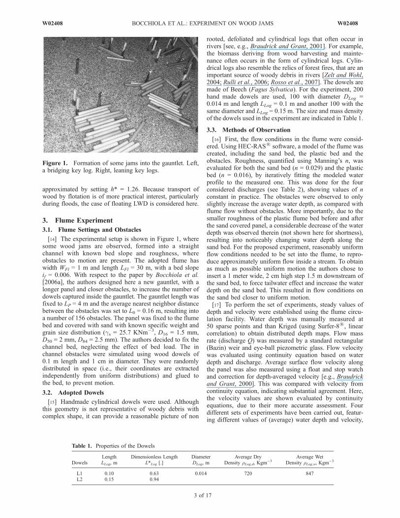
[14] The experimental setup is shown in Figure 1, wheresome wood jams are observed, formed into a straightchannel with known bed slope and roughness, whereobstacles to motion are present. The adopted flume haswidth WFl = 1 m and length LFl = 30 m, with a bed slopeif = 0.006. With respect to the paper by Bocchiola et al.[2006a], the authors designed here a new gauntlet, with alonger panel and closer obstacles, to increase the number ofdowels captured inside the gauntlet. The gauntlet length wasfixed to LP = 4 m and the average nearest neighbor distancebetween the obstacles was set to L0 = 0.16 m, resulting intoa number of 156 obstacles. The panel was fixed to the flumebed and covered with sand with known specific weight andgrain size distribution (gs = 25.7 KNm�3, D16 = 1.5 mm,D50 = 2 mm, D84 = 2.5 mm). The authors decided to fix thechannel bed, neglecting the effect of bed load. The inchannel obstacles were simulated using wood dowels of0.1 m length and 1 cm in diameter. They were randomlydistributed in space (i.e., their coordinates are extractedindependently from uniform distributions) and glued tothe bed, to prevent motion.

3.2. Adopted Dowels

[15] Handmade cylindrical dowels were used. Althoughthis geometry is not representative of woody debris withcomplex shape, it can provide a reasonable picture of non

rooted, defoliated and cylindrical logs that often occur inrivers [see, e.g., Braudrick and Grant, 2001]. For example,the biomass deriving from wood harvesting and mainte-nance often occurs in the form of cylindrical logs. Cylin-drical logs also resemble the relics of forest fires, that are animportant source of woody debris in rivers [Zelt and Wohl,2004; Rulli et al., 2006; Rosso et al., 2007]. The dowels aremade of Beech (Fagus Sylvatica). For the experiment, 200hand made dowels are used, 100 with diameter DLog =0.014 m and length LLog = 0.1 m and another 100 with thesame diameter and LLog = 0.15 m. The size and mass densityof the dowels used in the experiment are indicated in Table 1.

3.3. Methods of Observation

[16] First, the flow conditions in the flume were consid-ered. Using HEC-RAS1 software, a model of the flume wascreated, including the sand bed, the plastic bed and theobstacles. Roughness, quantified using Manning’s n, wasevaluated for both the sand bed (n = 0.029) and the plasticbed (n = 0.016), by iteratively fitting the modeled waterprofile to the measured one. This was done for the fourconsidered discharges (see Table 2), showing values of nconstant in practice. The obstacles were observed to onlyslightly increase the average water depth, as compared withflume flow without obstacles. More importantly, due to thesmaller roughness of the plastic flume bed before and afterthe sand covered panel, a considerable decrease of the waterdepth was observed therein (not shown here for shortness),resulting into noticeably changing water depth along thesand bed. For the proposed experiment, reasonably uniformflow conditions needed to be set into the flume, to repro-duce approximately uniform flow inside a stream. To obtainas much as possible uniform motion the authors chose toinsert a 1 meter wide, 2 cm high step 1.5 m downstream ofthe sand bed, to force tailwater effect and increase the waterdepth on the sand bed. This resulted in flow conditions onthe sand bed closer to uniform motion.[17] To perform the set of experiments, steady values of

depth and velocity were established using the flume circu-lation facility. Water depth was manually measured at50 sparse points and than Kriged (using Surfer-81, linearcorrelation) to obtain distributed depth maps. Flow massrate (discharge Q) was measured by a standard rectangular(Bazin) weir and eye-ball piezometric glass. Flow velocitywas evaluated using continuity equation based on waterdepth and discharge. Average surface flow velocity alongthe panel was also measured using a float and stop watchand correction for depth-averaged velocity [e.g., Braudrickand Grant, 2000]. This was compared with velocity fromcontinuity equation, indicating substantial agreement. Here,the velocity values are shown evaluated by continuityequations, due to their more accurate assessment. Fourdifferent sets of experiments have been carried out, featur-ing different values of (average) water depth and velocity,

Figure 1. Formation of some jams into the gauntlet. Left,a bridging key log. Right, leaning key logs.

Table 1. Properties of the Dowels

DowelsLengthLLog, m

Dimensionless LengthL*Log [.]

DiameterDLog, m

Average DryDensity rLog,d, Kgm

�3Average Wet

Density rLog,w, Kgm�3

L1 0.10 0.63 0.014 720 847L2 0.15 0.94

W02408 BOCCHIOLA ET AL.: EXPERIMENT ON WOOD JAMS

3 of 17

W02408

indicated in Table 2. A comprehensive description of theflow conditions is shown in Figure 2. Therein, the average(cross section) flow conditions along the sand bed areshown. These are the water depth dw in cm obtained by

averaging of the Kriged maps, its average value along thepanel dwav and the corresponding depth for uniform flowdw0. Notice that a horizontal line for dw indicates uniformflow. Also, the energy line is shown H (in cm, with level

Table 2. Summary of the Experimental Flow Conditions

Water Depth Dowel Q [ls�1] dwav cm Uwav ms�1 Re [.] Fr [.] ReLog [.] FrLog [.] h* [.]

H1 2.8 1.58 0.18 1.0E + 04 0.46 2.3E + 03 0.49 1.33H2 5.6 2.45 0.23 2.0E + 04 0.46 2.9E + 03 0.61 2.07H3 9.9 3.52 0.28 3.6E + 04 0.48 3.6E + 03 0.76 2.97H4 15.9 4.69 0.34 6.0E + 04 0.51 4.4E + 03 0.93 3.96

Figure 2. Hydraulic conditions in the experiments. From top-down, H1, H2, H3, H4. dw is water depth,dwav is average water depth value along the panel and dw0 is depth for uniform flow. H is energy line withlevel zero as referred to the last cross section, L = 4 m, H0 is energy line for uniform flow. U is velocity(secondary axis).

4 of 17

W02408 BOCCHIOLA ET AL.: EXPERIMENT ON WOOD JAMS W02408

zero as referred to the last cross section, L = 4 m), togetherwith the energy line for uniform flow H0. Here, uniformflow is no more represented by a horizontal line, but insteadby a line with constant slope (i.e., the friction slope). This isbecause the kinetic head Uw

2 /2g amounts to few millimeters,due to low velocity (see Table 2), thus making difficult tovisualize water surface (dw) and energy line (dw + U2/2g) inthe same scale. Also water velocity (secondary axis) isreported.[18] Although the flow conditions are variable along the

plate, the deviation from uniform flow seems acceptable.The greatest relative deviation of dw from dw0 amounts to21% for the inlet section in case H2, while the averagedepth dwav never differs from dw0 for more than 2%, in caseH3. Therefore the authors feel confident in considering asthe representative depth and velocity, the average value dwavand Uwav = Q/dwav.[19] Each set of experiments was composed of 2 trials,

corresponding to two different lengths of the dowels,namely L1 = 0.10 m and L2 = 0.15 m. Each trial wasrepeated four times, for more statistical robustness. Eachrepetition was carried out by sequentially inserting a num-ber of 100 dowels perpendicularly to main flow direction.To mimic a random effect with respect to the position of theobstacles, 5 starting positions inside the flume were con-sidered (i.e., 5 different values of the abscissa x in Figure 3,identified as A, B, C, D and E) far 15 cm from each otherand 20 cm away from the walls. Because the dowels wouldmove by floating with their axes parallel to flow, they wouldnot touch the flume walls easily and a distance of 20 cm wasobserved to be sufficient to avoid side effects. When adowel stops and reaches a visually steady position, anotherdowel is inserted. When all the 100 dowels have beeninserted and have reached their final setting, their positionsis mapped and another repetition is carried out. After fourrepetitions, another trial is carried out, by changing dowels’length. Eventually, a number of 32 repetitions was carriedout (i.e., considering four flow depths, two log lengths andfour repetitions), for a grand total of 3200 mapped dowels.[20] A jam is formed when a number of pieces are

grouped together so that the all pieces are in touch. Foreach jam, the forming key log is found and classifiedaccording to the different stopping mode, i.e., by leaning,Le, or bridging, Br. Although in some cases this operation issomewhat subjective, particularly when a high number oflogs is observed, in most of the cases the key log is clearlyidentified. Also, the experiments were filmed using a digitalcamera, so aiding in the identification of the key logs in caseof doubts.[21] The choice of using 100 dowels is arbitrary. For

instance, one could consider a number of pieces necessaryto reach some equilibrium conditions in the stream, e.g.,when the number of dowels incoming over a referenceperiod is equal to the number of those running out of theflume. In real rivers the reference period would probably belinked to the average rate of supply of wood pieces (e.g.,pieces/day). For rivers with a high supply rate, this means ashort period (e.g., few days), while for low supply rate, thiscould mean a long period (e.g., months). In turn, the supplyrate is related to the occurrence of relevant storms, increas-ing abruptly the amount of wood conveyed into the channel

[e.g., Kraft and Warren, 2003], but also sweeping away theaccumulated wood pieces. When relatively long term accu-mulation is considered, wood decay would also affect theaccumulation of wood. Therefore a quantitative assessmentof the dynamic equilibrium of a stream and the timescaletherein, that should be then reproduced at the flume scaleseems complicate and the authors are not aware of any suchattempt in practice.[22] The present results simply mimic the behavior of a

stream that is initially empty, after a number of 100 dowel isinserted, that seems to describe in a first approximation thedynamics of jamming into a river. In the future, moreexperiment could be carried out to investigate the issue ofdynamic equilibrium.[23] The experiment of uncongested transport was carried

out in the same hydraulic conditions. For each velocity anddowels’ length a trial was carried out. For each trial, at thestarting positions (A, B, C, D, E), ten dowels were sequen-tially inserted in the flow and subsequently removed.Eventually, 8 trials were carried out, for a total of 400mapped dowels.

3.4. Scaling Issues

[24] Dimensional analysis indicates that the experimentmimics transport of wood pieces in mountain streams within channel boulders or vegetation, in braided rivers or infloodplains during flood events. First, one has to considerthe Froude number Fr = Uw/(gdw)

0.5, with g gravity accel-eration and the Reynolds number, Re = 4Uwdw/n, with nkinematic viscosity (see Table 2). The former ranges from0.46 to 0.51, while the latter ranges from 1E4 to 6E4. Theseprovide conditions similar to those observed for low waterdepths, when interaction with wood is of interest [see, e.g.,Braudrick and Grant, 2000, Table 3]. To provide similarityat the field scale, both Re and Fr should be maintained. Thiscannot be done when working with the same fluid (i.e.,water). According to, e.g., Wallerstein et al. [2001] resistiveforces scale logarithmically with Reynolds number andbecome in practice constant for turbulent flows, albeit notfully developed as here. Therefore Reynolds scaling can berelaxed in a first approximation. As far as the LWD isconcerned, the scaling was described by Bocchiola et al.[2006a] and requires some changes here. In plane, similarityholds provided the ratio between LWD length and obstaclesspacing L*Log = LLog/L0 is maintained. The scaling in thevertical direction depends on LWD motion conditions.When LWD is in touch with bed the scaling is dictated bythe (dimensionless) excess of force acting on the woodpiece, with respect to the threshold for motion. When LWDfloats, a null threshold occurs, because the wood is no morein touch with the bed. In the simplified hypothesis thatLWD moves at flow velocity (see, e.g., Braudrick andGrant, 2001), dimensional analysis (Biesuz and Zanetti,2005, not shown here for shortness) show that the scalingparameters are the Froude and Reynolds number of the log,FrLog = Uw/(g Dlog)

0.5 and ReLog = Uw DLog/n [see alsoWallerstein et al., 2001]. Particularly, FrLog and ReLog affectthe value of drag coefficient, so influencing the interactionof wood and flowing water [Wallerstein et al., 2002]. Here,ReLog ranges from 2.3E + 03 to 4.4 E + 03. The dragcoefficient is practically constant against ReLog for values ofthe latter up 1E6 [e.g., Wallerstein et al., 2001; Alonso,

W02408 BOCCHIOLA ET AL.: EXPERIMENT ON WOOD JAMS

5 of 17

W02408

2004] and Reynolds scaling can therefore be relaxed in afirst approximation. The Froude number of the logs FrLogranges here from 0.21 to 0.86, showing instead moreinfluence [e.g., Alonso, 2004]. Also, considerable valuesof the blockage of single wood pieces with respect to theflow area, B = DLog LLog/WFl dw affect the drag coefficient[e.g., Shields and Gippel, 1995]. However, B is quite lowhere, as it ranges from 0.03 to 0.13, thus providing nopractical influence on the results [e.g., Hygelund and

Manga, 2003]. Therefore the parameters dictating the scal-ing is here FrLog.

4. Experimental Results

4.1. Motion Patterns and Quantitative Description ofthe Jams

[25] The dowels quickly self-adjust their direction tomatch the flow direction and converge toward the center-

Figure 3. Distribution of the jams for L1. Average on four repetitions. Number of pieces rounded tonearest integer.

6 of 17

W02408 BOCCHIOLA ET AL.: EXPERIMENT ON WOOD JAMS W02408

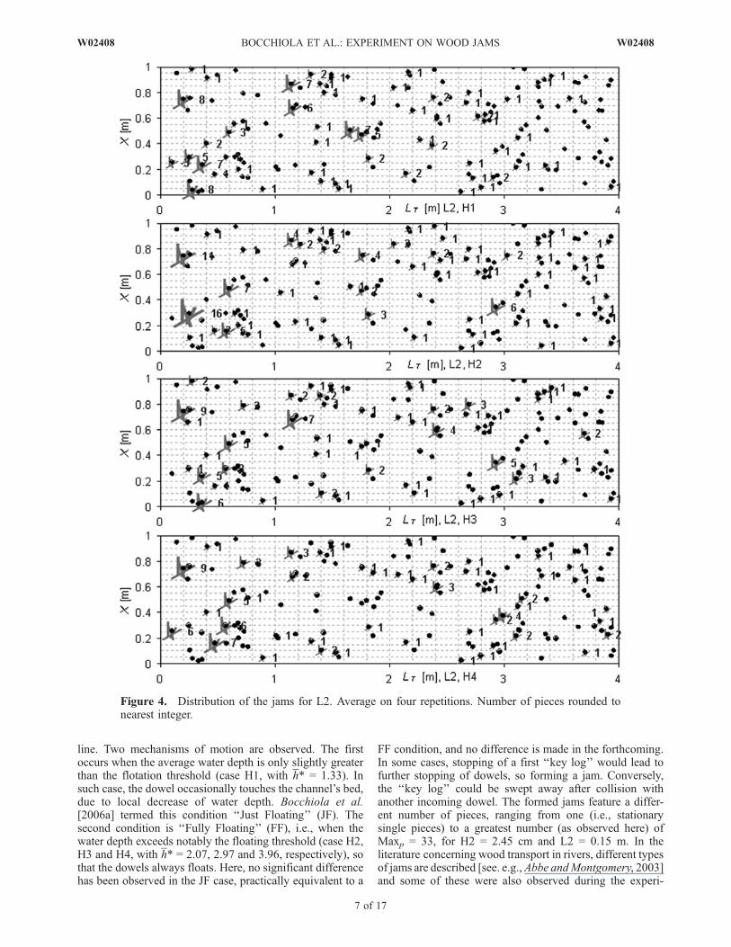
line. Two mechanisms of motion are observed. The firstoccurs when the average water depth is only slightly greaterthan the flotation threshold (case H1, with h* = 1.33). Insuch case, the dowel occasionally touches the channel’s bed,due to local decrease of water depth. Bocchiola et al.[2006a] termed this condition ‘‘Just Floating’’ (JF). Thesecond condition is ‘‘Fully Floating’’ (FF), i.e., when thewater depth exceeds notably the floating threshold (case H2,H3 and H4, with h* = 2.07, 2.97 and 3.96, respectively), sothat the dowels always floats. Here, no significant differencehas been observed in the JF case, practically equivalent to a

FF condition, and no difference is made in the forthcoming.In some cases, stopping of a first ‘‘key log’’ would lead tofurther stopping of dowels, so forming a jam. Conversely,the ‘‘key log’’ could be swept away after collision withanother incoming dowel. The formed jams feature a differ-ent number of pieces, ranging from one (i.e., stationarysingle pieces) to a greatest number (as observed here) ofMaxp = 33, for H2 = 2.45 cm and L2 = 0.15 m. In theliterature concerning wood transport in rivers, different typesof jams are described [see. e.g.,Abbe andMontgomery, 2003]and some of these were also observed during the experi-

Figure 4. Distribution of the jams for L2. Average on four repetitions. Number of pieces rounded tonearest integer.

W02408 BOCCHIOLA ET AL.: EXPERIMENT ON WOOD JAMS

7 of 17

W02408

ment. However, jams type classification is strictly linked toriver morphology, including lateral constriction, bends,vertical structures (steps, pool), floodplains and the presenceof bed load. Because here such phenomena are not repre-sented and therefore comparison would be difficult, theauthors make here no distinctions between different types ofjams and focus is directed on the number of pieces. InFigures 3 and 4 visual summary of the experiments is given.Therein, for each couple of H and L, the position and size ofthe formed jams are given. The number of dowels in a jamis reported for each obstacle. This is the average value of thenumber of dowels that was observed in each of the fourrepetitions for given flow depth and log length, rounded tothe nearest integer.[26] In Table 3, a quantitative description of the results is

given. First, the number of jams NJ is reported, averagedover the four repetition and rounded to the nearest integer.Then, the greatest number of dowels in a jam is reported forone single repetition, Maxp, together with its average on thefour repetitions, Maxpav. NJ is shown in Figure 5 against

FrLog. The number of jams NJ slightly decreases with FrLog,particularly for L1.[27] The average E[Np] and the coefficient of variation

CV[Np], i.e., the ratio between standard deviation andaverage value, of the number of pieces into the jams arealso reported in Table 3. E[Np], in Figure 5, is higher for L2.The fraction of stopping dowels inside the gauntlet is given,StopJ, together with that of the jams formed by a bridgingkey log, BrJ (the fraction of leaning key logs is LeJ = 1 �BrJ). These values can be compared with those for uncon-gested transport, Stops and Brs also reported in Table 3. Thecomparison is shown in Figures 6 and 7. Generally speak-ing, the probability of a log to be trapped increases with itslength and decreases with flow velocity (scaled to logdiameter, as given by FrLog). Here, it is shown that theprobability of stopping is higher for single logs than forjams, as evaluated in steady state (i.e., after each repetition)condition.[28] One can define a removal rate, Rem = 1 � StopJ/

Stops, measuring the degree of removal of trapped (key)logs due to flow conditions. This is reported in Table 3 andincreases with FrLog. This is due to removal of lodged logsafter collision with moving logs. As a final result, thefraction of retained logs inside the channel is smaller thanthat of retained logs (i.e., the probability of stopping) whenuncongested transport is observed. Also, one can define anefficiency of trapping

EffType ¼StopJ TypeJ � Stops Typesð Þ

Stops Types; ð1Þ

with Type either Br or Le. Eff can be either positive ornegative, the former case indicating a higher fraction ofwood pieces in jams retained in mode Type than in the caseof single pieces, and the latter case the vice versa. Eff isgiven in Table 3. As expected, this is positive (and slightlydecreasing with FrLog) for Br and negative (quite constantwith FrLog) for Le. The efficiency of bridging, EffBr is highfor L1 when low values of FrLog are observed (EffBr = 2 orso), but drops noticeably for increasing FrLog (EffBr = 0.08or so). Accordingly, logs tend to stick for low velocity, butare swept away for high velocity. For L2, EffBr depends

Table 3. Summary of the Experimental Results

Forcing L1 L2

Dowel H1 H2 H3 H4 H1 H2 H3 H4

NJ [.] 31 27 21 17 23 21 22 19Maxp [.] 15 12 12 17 32 33 24 25Maxpav [.] 10 10 9 11 23 22 16 17E[Np] [.] 2.80 2.75 2.88 3.13 4.19 4.49 3.85 4.22CV[Np] [.] 0.84 0.85 0.80 0.85 1.32 1.15 1.14 1.05StopJ [.] 0.86 0.74 0.60 0.53 0.97 0.91 0.83 0.78BrJ [.] 0.63 0.59 0.70 0.76 0.81 0.95 0.85 0.83Stops [.] 0.96 0.88 0.68 0.67 0.100 0.96 0.94 0.86Brs [.] 0.18 0.33 0.53 0.56 0.51 0.69 0.58 0.61Rem [.] 0.10 0.16 0.12 0.21 0.03 0.05 0.12 0.10EffBr [.] 2.05 0.50 0.16 0.08 0.54 0.30 0.29 0.21EffLe [.] �0.59 �0.48 �0.43 �0.57 �0.63 �0.84 �0.69 �0.60E[L*T]J [.] 14.62 16.20 21.16 23.96 12.92 13.72 15.23 16.63CV[LT*]J [.] 0.58 0.58 0.58 0.58 0.58 0.58 0.58 0.58E[L*T]s [.] 8.71 12.85 15.78 20.45 7.70 9.74 10.20 12.94CV[LT*]s [.] 0.81 0.82 0.79 0.77 0.83 0.87 0.89 0.93E[L*T]w [.] 13.00 18.73 25.88 30.37 8.94 11.22 17.40 18.03CV[LT*]w [.] 0.73 0.76 0.83 0.87 0.79 0.91 0.87 0.94r [.] �0.34 �0.23 �0.23 �0.34 �0.42 �0.42 �0.45 �0.36

Figure 5. Number of jams and average number of wood pieces in a jam, against FrLog.

8 of 17

W02408 BOCCHIOLA ET AL.: EXPERIMENT ON WOOD JAMS W02408

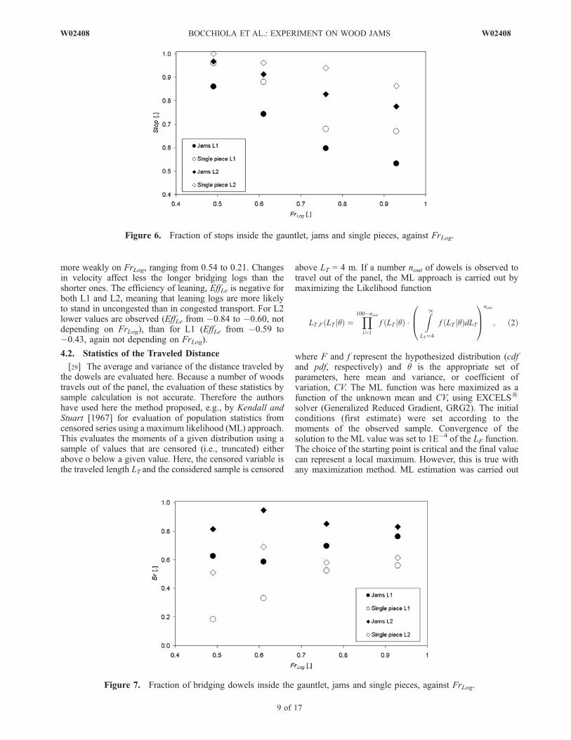
more weakly on FrLog, ranging from 0.54 to 0.21. Changesin velocity affect less the longer bridging logs than theshorter ones. The efficiency of leaning, EffLe is negative forboth L1 and L2, meaning that leaning logs are more likelyto stand in uncongested than in congested transport. For L2lower values are observed (EffLe from �0.84 to �0.60, notdepending on FrLog), than for L1 (EffLe from �0.59 to�0.43, again not depending on FrLog).

4.2. Statistics of the Traveled Distance

[29] The average and variance of the distance traveled bythe dowels are evaluated here. Because a number of woodstravels out of the panel, the evaluation of these statistics bysample calculation is not accurate. Therefore the authorshave used here the method proposed, e.g., by Kendall andStuart [1967] for evaluation of population statistics fromcensored series using a maximum likelihood (ML) approach.This evaluates the moments of a given distribution using asample of values that are censored (i.e., truncated) eitherabove o below a given value. Here, the censored variable isthe traveled length LT and the considered sample is censored

above LT = 4 m. If a number nout of dowels is observed totravel out of the panel, the ML approach is carried out bymaximizing the Likelihood function

LT ;F LT jqð Þ ¼Y100�nout

i¼1

f LT jqð Þ �Z1

LT¼4

f LT jqð ÞdLT

0B@

1CA

nout

; ð2Þ

where F and f represent the hypothesized distribution (cdfand pdf, respectively) and q is the appropriate set ofparameters, here mean and variance, or coefficient ofvariation, CV. The ML function was here maximized as afunction of the unknown mean and CV, using EXCELS1

solver (Generalized Reduced Gradient, GRG2). The initialconditions (first estimate) were set according to themoments of the observed sample. Convergence of thesolution to the ML value was set to 1E�4 of the LF function.The choice of the starting point is critical and the final valuecan represent a local maximum. However, this is true withany maximization method. ML estimation was carried out

Figure 6. Fraction of stops inside the gauntlet, jams and single pieces, against FrLog.

Figure 7. Fraction of bridging dowels inside the gauntlet, jams and single pieces, against FrLog.

W02408 BOCCHIOLA ET AL.: EXPERIMENT ON WOOD JAMS

9 of 17

W02408

for each of the four repetitions and the values so obtainedwere compared to each other for consistency. In all cases,consistent results were found (not shown for shortness). Thevalues of mean and variance obtained from averaging of thefour repetitions are reported in Table 3. To carry out the MLfunction, a preliminary assessment of the F function isrequired. For each of the variables considered here,preliminary testing was carried out using five standarddistributions, namely Uniform (UN), Exponential (EXP),Normal (NR), Lognormal (LN) and Gamma (GA). Thedistribution was chosen giving the best (eyeball) fitting tothe observed data. The so obtained distributions are shownin the next section. In the following, the traveled distance isconsidered made dimensionless with respect to L0, or L*T =LT/L0. This is consistent with scaling LLog to L0 and allowsto use geometric similarity in field studies or flumeexperiments. First, the average distance of the jams fromthe channel inlet E[L*T]J is calculated, together with itscoefficient of variation CV[L*T]J. Notice that the MLestimation showed a Uniform distribution of L*T of jams, so

giving CV[L*T]J = 0.58. Then, the same statistics arecalculated considering the single pieces of wood into thejams, namely E[L*T]w and CV[L*T]w. Also, these statisticsare calculated in the case of uncongested transport (i.e.,single woods), E[L*T]s and CV[L*T]s. The values of E[L*T]are shown in Figure 8. E[L*T] is smaller for single piecesthan for the jams, due to wood redistribution duringcongested transport. Also, E[L*T] is higher for single piecesin jams, than their counterpart for uncongested transport.Notice also that E[L*T] increases with FrLog, while CV[L*T]seems only slightly variable against FrLog (see Table 3).

4.3. Frequency Distributions of the Traveled Distanceand the Jams Size

[30] The frequency distributions resulting from the MLapproach are reported here. Also the distribution of Np isstudied. For the latter only sample statistics are used, in thereasonable hypothesis that the wood pieces running outsidethe gauntlet do not change substantially the size of the jams.Here, the sample values obtained for different values of

Figure 8. Average distance traveled inside the gauntlet for jams, wood pieces in jams and single pieces,against FrLog. (a) L1. (b) L2.

10 of 17

W02408 BOCCHIOLA ET AL.: EXPERIMENT ON WOOD JAMS W02408

FrLog were made dimensionless with respect to their aver-age, as follows

L0T ¼ L*T

E L*T

h i ; N 0p ¼

Np

E Np

� � : ð3Þ

This allows distribution fitting by using the sample obtainedby grouping together the values of L0T and N0

p for thedifferent values of FrLog. This is tantamount to assume thatdifferent values of FrLog can influence the average traveledlength and its standard deviation, but the ratio between thelatter and the former, i.e., the CV remains more or lessconstant. Strictly speaking, this procedure is allowed if thedistribution of the dimensionless values is equivalent foreach value of FrLog, i.e., if it shows the same coefficient ofvariation CV. Analysis of the estimatedCV values, in Table 3,shows only slight dependence of the latter upon the value ofFrLog. More influence is given by the dowels length,because the CV value for L1 is lower than for L2. On aprinciple line, some statistical tests should be carried out toassess homogeneity of the CV coefficients. Here, due to thevery preliminary nature of the proposed attempt, equiva-lence of the CV values with respect to FrLog is tentativelyassumed. Also, plotting positions of the observed frequen-

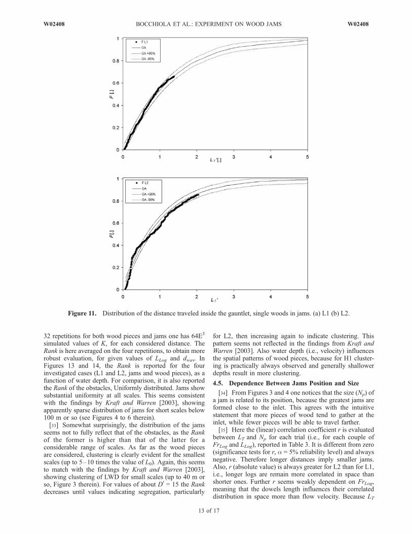
cies was preliminarily carried out (not shown here forshortness), showing indeed no relevant visual difference.Distribution fitting is instead carried out separately for thetwo different log lengths. The observed frequency distribu-tions so obtained are shown in Figures 9 (a for L1, b for L2),10 (a for L1, b for L2), 11 (a for L1, b for L2), and 12 (a forL1, b for L2) for single logs, jams, single pieces in jams andjams size, respectively.[31] Therein it is shown the probability (evaluated using

Weibull plotting position, F = n/(ntot + 1), with n rank of thesample in the series ordered in decreasing order and ntotwhole sample size) that a piece (or a jam) is positionedwithin a given traveled distance L0T, or that a jam is madeof a given number of elements smaller or equal to N0

p. Forthe traveled length, the plotting position is compared to thestandard distribution used for the ML approach. No testfor distribution fitting is carried out here and only confi-dence limits are given to aid goodness of fit evaluation(Kolmogorov Smirnov, a = 5%). Best fitting to the observedtraveled distance L0T of the single pieces is given by GA,with more scatter for L2. Notice that the scatterplot showsfrequencies lower than one, as a result of the censoring forhigh values of L0T (i.e., for LT > 4m). The traveled distance ofjams is distributed according to an UN. The single pieces in

Figure 9. Distribution of the distance traveled inside the gauntlet, single pieces. (a) L1 (b) L2.

W02408 BOCCHIOLA ET AL.: EXPERIMENT ON WOOD JAMS

11 of 17

W02408

jams are well represented by a GA, again with more scatterfor length L2, apparently consistent with the GA distributionfor single pieces. Eventually, the frequency of N0

p is reason-ably well accommodated by an EXP distribution. Worsefitting is observed for L2, but the EXP seems to capture thecore of the scatterplot.

4.4. Neighbor K Statistics for the Jams and the WoodPieces

[32] To emphasize the attitude, if any, of the wood piecesto either cluster or segregate at given spatial scales, neigh-bor K statistics are here calculated. The same approachproposed by Kraft and Warren [2003] is used. In short, theK statistic evaluates the number of wood pieces (or jams)within a given distance from another wood piece (or jam),averaged on the whole sample

K Dð Þ ¼ 1

ns

Xi 6¼j

Xi 6¼j

ID xij� �

; ð4Þ

with ns sample size, xij distance between samples i and j,and ID = 0 if xij > D; ID = 1 if xij D. Distance D representsthe scale at which the degree of sparseness is tested.

Calculation of K is here carried out for each repetition of theexperiment. Then, the Rank (i.e., frequency of exceedance)of K is calculated. This indicates the chance that the value ofK obtained for a given distance is representative of auniform distribution. To evaluate the Rank, a referencestatistic is needed, based on Monte Carlo approach. Foreach repetition, a number of 1000 equivalent syntheticsimulations is carried out, considering the same number ofjams, or wood pieces as observed. Each simulation providesa possible distribution in space that would be obtained if thecoordinates of the jams or the wood pieces were extractedfrom uniform random variables (i.e., if they were uniformlydistributed in space). For each of the synthetic distributions,the value of K(D) is estimated. The values of K(D) soobtained is Normally distributed [e.g., Kraft and Warren,2003]. Using this Normal distribution, the Rank of theobserved value of K(D) is evaluated. Taking a confidencelevel a = 5%, the Rank can indicate either clustering(Rank > 0.975) or segregation (Rank < 0.025). Here, thedistance is considered made dimensionless with respect toL0, or D

0 = D/L0, so that the proposed results can be scaled toobstacles spacing. The physical extent tested is from D =0.05 m, toD = LP = 4 m, that is the greatest possible distancebetween the jams, with steps of 0.05 m. Considering

Figure 10. Distribution of the distance traveled inside the gauntlet, jams. (a) L1 (b) L2.

12 of 17

W02408 BOCCHIOLA ET AL.: EXPERIMENT ON WOOD JAMS W02408

32 repetitions for both wood pieces and jams one has 64E3

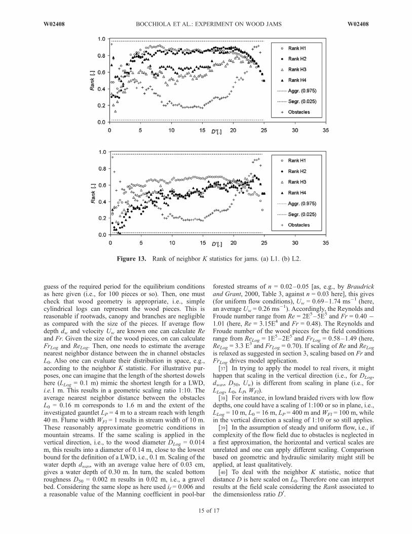
simulated values of K, for each considered distance. TheRank is here averaged on the four repetitions, to obtain morerobust evaluation, for given values of LLog and dwav. InFigures 13 and 14, the Rank is reported for the fourinvestigated cases (L1 and L2, jams and wood pieces), as afunction of water depth. For comparison, it is also reportedthe Rank of the obstacles, Uniformly distributed. Jams showsubstantial uniformity at all scales. This seems consistentwith the findings by Kraft and Warren [2003], showingapparently sparse distribution of jams for short scales below100 m or so (see Figures 4 to 6 therein).[33] Somewhat surprisingly, the distribution of the jams

seems not to fully reflect that of the obstacles, as the Rankof the former is higher than that of the latter for aconsiderable range of scales. As far as the wood piecesare considered, clustering is clearly evident for the smallestscales (up to 5–10 times the value of L0). Again, this seemsto match with the findings by Kraft and Warren [2003],showing clustering of LWD for small scales (up to 40 m orso, Figure 3 therein). For values of about D0 = 15 the Rankdecreases until values indicating segregation, particularly

for L2, then increasing again to indicate clustering. Thispattern seems not reflected in the findings from Kraft andWarren [2003]. Also water depth (i.e., velocity) influencesthe spatial patterns of wood pieces, because for H1 cluster-ing is practically always observed and generally shallowerdepths result in more clustering.

4.5. Dependence Between Jams Position and Size

[34] From Figures 3 and 4 one notices that the size (Np) ofa jam is related to its position, because the greatest jams areformed close to the inlet. This agrees with the intuitivestatement that more pieces of wood tend to gather at theinlet, while fewer pieces will be able to travel farther.[35] Here the (linear) correlation coefficient r is evaluated

between LT and Np for each trial (i.e., for each couple ofFrLog and LLog), reported in Table 3. It is different from zero(significance tests for r, a = 5% reliability level) and alwaysnegative. Therefore longer distances imply smaller jams.Also, r (absolute value) is always greater for L2 than for L1,i.e., longer logs are remain more correlated in space thanshorter ones. Further r seems weakly dependent on FrLog,meaning that the dowels length influences their correlateddistribution in space more than flow velocity. Because LT

Figure 11. Distribution of the distance traveled inside the gauntlet, single woods in jams. (a) L1 (b) L2.

W02408 BOCCHIOLA ET AL.: EXPERIMENT ON WOOD JAMS

13 of 17

W02408

and Np are likely to be significantly correlated, their jointdistribution is different from the product of the two marginaldistributions and should be carried out according to abivariate approach [e.g., Kottegoda and Rosso, 1997, Ch. 3].The latter is possibly a research issue in itself and goesbeyond the scopes of the present paper. A more refinedapproach including for instance bivariate distribution fittingor copulas could be used in the future to model theaccumulation process of jams, in turn increasing therequired experimental effort, because bivariate approachesclaim for considerable sample dimensionality for robustmodel estimation.

5. Discussion of Model Application in Real Rivers

[36] A number of field campaigns have been carried outin the near past to evaluate the patterns of deposition ofwood in streams (among others, it is worth quoting here theworks by Prof. Angela Gurnell and her team, concerning theTagliamento river, in Italy, reported in the references).Accumulation patterns of wood are qualitatively described,in some cases with specific reference to stream geometry [as,e.g., by Jackson and Sturm, 2002; Abbe and Montgomery,2003], but usually with no modeling purposes. In this sense,

the present experiment sketches a simple model to assessthe statistical distribution and degree of aggregation ofwood pieces in streams for predictive purposes. Modelapplication is not straightforward, in view of the utmostcomplexity of the interaction between wood accumulationpatterns and flow in streams. However, it is possible to drawhere some guidelines for a qualitative comparison of theproposed flume scale results against findings of equivalentfield experiments, based on similarity of geometric andhydraulic conditions. First, one has to consider relativelylow flow depths in respect to wood size, or h* � 1–5 andcontrol provided by bed geometry, in presence, e.g., ofboulders in mountain streams [as, e.g., by Kraft and Warren,2003] or bars in braided rivers [as, e.g., by Gurnell et al.,2000a]. Relative low blockage should be considered ashere, or B � 0.01–0.2, i.e., small wood pieces as comparedto flow area. Uncongested and congested transport can bediscriminated according to the observed degree of interac-tion between wood pieces. A small number of jams (eval-uated as, e.g., NJ/WFlLP) as compared to those reported heresuggests use of uncongested hypothesis, while more jamssuggests vice versa. Also, an average wood feeding rate(e.g., wood pieces per day) can be assessed, providing a first

Figure 12. Distribution of the number of wood pieces. (a) L1 (b) L2.

14 of 17

W02408 BOCCHIOLA ET AL.: EXPERIMENT ON WOOD JAMS W02408

guess of the required period for the equilibrium conditionsas here given (i.e., for 100 pieces or so). Then, one mustcheck that wood geometry is appropriate, i.e., simplecylindrical logs can represent the wood pieces. This isreasonable if rootwads, canopy and branches are negligibleas compared with the size of the pieces. If average flowdepth dw and velocity Uw are known one can calculate Reand Fr. Given the size of the wood pieces, on can calculateFrLog and ReLog. Then, one needs to estimate the averagenearest neighbor distance between the in channel obstaclesL0. Also one can evaluate their distribution in space, e.g.,according to the neighbor K statistic. For illustrative pur-poses, one can imagine that the length of the shortest dowelshere (LLog = 0.1 m) mimic the shortest length for a LWD,i.e.1 m. This results in a geometric scaling ratio 1:10. Theaverage nearest neighbor distance between the obstaclesL0 = 0.16 m corresponds to 1.6 m and the extent of theinvestigated gauntlet LP = 4 m to a stream reach with length40 m. Flume width WFl = 1 results in stream width of 10 m.These reasonably approximate geometric conditions inmountain streams. If the same scaling is applied in thevertical direction, i.e., to the wood diameter DLog = 0.014m, this results into a diameter of 0.14 m, close to the lowestbound for the definition of a LWD, i.e., 0.1 m. Scaling of thewater depth dwav, with an average value here of 0.03 cm,gives a water depth of 0.30 m. In turn, the scaled bottomroughness D50 = 0.002 m results in 0.02 m, i.e., a gravelbed. Considering the same slope as here used if = 0.006 anda reasonable value of the Manning coefficient in pool-bar

forested streams of n = 0.02–0.05 [as, e.g., by Braudrickand Grant, 2000, Table 3, against n = 0.03 here], this gives(for uniform flow conditions), Uw = 0.69–1.74 ms�1 (here,an average Uw = 0.26 ms�1). Accordingly, the Reynolds andFroude number range from Re = 2E5–5E5 and Fr = 0.40 �1.01 (here, Re = 3.15E4 and Fr = 0.48). The Reynolds andFroude number of the wood pieces for the field conditionsrange from ReLog = 1E5–2E5 and FrLog = 0.58–1.49 (here,ReLog = 3.3 E3 and FrLog = 0.70). If scaling of Re and ReLogis relaxed as suggested in section 3, scaling based on Fr andFrLog drives model application.[37] In trying to apply the model to real rivers, it might

happen that scaling in the vertical direction (i.e., for DLog,dwav, D50, Uw) is different from scaling in plane (i.e., forLLog, L0, LP, WFl).[38] For instance, in lowland braided rivers with low flow

depths, one could have a scaling of 1:100 or so in plane, i.e.,LLog = 10 m, L0 = 16 m, LP = 400 m andWFl = 100 m, whilein the vertical direction a scaling of 1:10 or so still applies.[39] In the assumption of steady and uniform flow, i.e., if

complexity of the flow field due to obstacles is neglected ina first approximation, the horizontal and vertical scales areunrelated and one can apply different scaling. Comparisonbased on geometric and hydraulic similarity might still beapplied, at least qualitatively.[40] To deal with the neighbor K statistic, notice that

distance D is here scaled on L0. Therefore one can interpretresults at the field scale considering the Rank associated tothe dimensionless ratio D0.

Figure 13. Rank of neighbor K statistics for jams. (a) L1. (b) L2.

W02408 BOCCHIOLA ET AL.: EXPERIMENT ON WOOD JAMS

15 of 17

W02408

[41] According to the guidelines her given, qualitativecomparison of either field or laboratory scale results againstthe model here proposed can be carried out. In doing so thesimplifying hypothesis here introduced should be reason-ably fulfilled and scaling respected. This results in rela-tively restrictive conditions as compared to the complexityobserved in real rivers, thus requiring care in modelapplication.

6. Conclusions

[42] The formation of wood jams in streams is a multi-faceted process, involving a combination of deterministicmechanisms and random factors. The present approachprovides a simplified sketch of LWD and stream flowsgeometry as a first attempt to represent such complexity, tobe developed henceforth. Some preliminary findings can bestressed. The probability that LWD is entrained in jamsincreases with its length and decreases with its Froudenumber. Trapping is more efficient if bridging against twoobstacles is likely, i.e., when obstacles are close comparedto LWD length. Congested transport leads LWD pieces tooccupy more extensively the available space than theywould do singularly, i.e., with little congestion. Theobserved frequency of the distance traveled by LWD andits quantitative aggregation (i.e., the number of pieces) canbe explained fairly well using proper statistical distribu-tions. Analysis using neighbor K statistic shows consider-able aggregation of the pieces of LWD, while sparseoccupation is attained by wood jams. Not surprisingly, there

is significant statistical linkage between jams size andtraveled distance, that is worth of more investigation maybeusing bivariate approach. The accumulation of LWD and theformation of wood structures influence river geomorpholo-gy and riverine environment quality, but also river convey-ance and hydraulic hazard, especially where man-madestructures yield supplementary obstacles to LWD. Theproposed statistical approach could be adopted as a basisto predict wood accumulation patterns for river managementpurposes, wood insertion for habitat restoration and evalu-ation of hazard for man-made structures, such as dams orbridges.[43] Further developments need to include the study of

more complex LWD geometry, including roots and foliage.Further, the accumulation process needs to be studied inmore complex (in field and flume scaled) stream geometry,including bends and braiding and vertical structure. Also,the presence of sediment load must be introduced, particu-larly relevant during flood events. Eventually, the proposedresults and the way they pave for future investigation seemof interest for researchers and river managers and cancontribute to the understanding of the interaction betweenvegetation and river geomorphology.

[44] Acknowledgments. The authors kindly acknowledge Eng. S.Biesuz and Eng. A. Zanetti, for their contribution to the presented research,in partial fulfillment of their master’s thesis. Giuseppe Passoni, at Politec-nico di Milano, is kindly acknowledged for fruitful discussion concerningscaling issues in stream flows. Jochen Aberle and three other anonymousreviewers are acknowledged for providing precious suggestions that guidedthe authors in making the paper more comprehensive and readable.

Figure 14. Rank of neighbor K statistics for wood pieces in jams. (a) L1. (b) L2.

16 of 17

W02408 BOCCHIOLA ET AL.: EXPERIMENT ON WOOD JAMS W02408

ReferencesAbbe, T. B., and D. R. Montgomery (1996), Large woody debris jams,channel hydraulics and habitat formation in large rivers, Reg. RiversRes. Manage., 12, 201–221.

Abbe, T. B., and D. R. Montgomery (2003), Patterns and processes of wooddebris accumulation in the Queets river basin, Washington, Geomorphol.,51, 81–107.

Alonso, C. V. (2004), Transport mechanics of stream-borne logs, Riparianvegetation and Fluvial Geomorphology, Water Science and Application8, AGU, 59–69.

Andrus, C.W., B.A. Long, and H.A. Froehlich (1988), Woody debris and itscontribution to pool formation in a costal stream 50 years after logging,Can. J. Fish. Aquat., 45, 2080–2086.

Aspinall, R. J. (2002), Use of logistic regression for validation of maps ofthe spatial distribution of vegetation species derived from high spatialresolution hyper spectral remotely sensed data, Ecological Modelling,157, 301–312.

Benda, L. E., and J. C. Sias (2003), A quantitative framework for evaluatingthe mass balance of in stream organic debris, For. Ecol. Manage. Else-vier, 172, 1–16.

Biesuz, S., and A. Zanetti (2005), Lodging of woody debris in channels:some experimental tests, Mater’s Thesis, Politecnico di Milano, Mat:643469, 644278. Tutor: R. Rosso. Cotutors: D. Bocchiola, M.C. Rulli.In Italian.

Bocchiola, D., F. Catalano, G. Menduni, and G. Passoni (2002), An analy-tical-numerical approach to the hydraulics of floating debris in riverchannels, J. Hydrol., 269(1–2), 65–78.

Bocchiola, D., M. C. Rulli, and R. Rosso (2006a), Transport of LargeWoody Debris in the presence of obstacles, Geomorphol., 76, 166–178.

Bocchiola, D., M. C. Rulli, and R. Rosso (2006b), Flume experiments onwood entrainment in rivers, Adv. Water Resour., 29(8), 1182–1195.

Braudrick, C. A., and G. E. Grant (2000), When do logs move in rivers?,Water Resour. Res., 36(2), 571–583.

Braudrick, C. A., and G. E. Grant (2001), Transport and deposition of largewoody debris in streams: A flume experiment, Geomorphol., 41, 263–283.

Braudrick, C. A., G. E. Grant, Y. Ishikawa, and H. Ikeda (1997), Dynamicsof wood transport in streams: A flume experiment, Earth Surf. ProcessesLandforms, 22, 669–683.

Faustini, J. M., and J. A. Jones (2003), Influence of large woody debris onchannel morphology and dynamics in steep, boulder-rich mountainstreams, western Cascades, Oregon, Geomorphol., 51, 187–205.

Fetherston, K. L., R. J. Naiman, and R. E. Bilby (1995), Large woodydebris, physical process and riparian forest development in montane rivernetworks of the Pacific Northwest, Geomorphol., 13, 133–144.

Gomi, T., R. C. Sidle, R. D. Woodsmith, and M. D. Bryant (2003), Char-acteristics of channel steps and reach morphology in headwater streamssoutheast Alaska, Geomorphol., 51, 225–242.

Gurnell, A. M., G. E. Petts, N. Harris, J. V. Ward, K. Tockner, P. J. Edwards,and J. Kollman (2000a), Large Wood retention in river channels: The caseof the Fiume Tagliamento, Italy, Earth Surf. Processes Landforms, 25,255–275.

Gurnell, A. M., G. E. Petts, D. M. Hannah, B. P. G. Smith, P. J. Edwards,J. Kollman, J. V. Ward, and K. Tockner (2000b), Wood storage within theactive zone of a large European gravel-bed river, Geomorphol., 34, 55–72.

Haga, H., T. Kumagai, K. Otsuki, and S. Ogawa (2002), Transport andretention of coarse woody debris in mountain streams: An in situ fieldexperiment of log transport and a field survey of coarse woody debrisdistribution,Water Resour. Res., 38(8), 1126, doi:10.1029/2001WR001123.

Hygelund, B., and M. Manga (2003), Field measurement of drag coeffi-cients for model large woody debris, Geomorphol., 51, 175–185.

Jackson, C. R., and C. A. Sturm (2002), Woody debris and channel mor-phology in first and second order forested channels in Washington’s coastranges, Water Resour. Res., 38(9), 1177, doi:10.1029/2001WR001138.

Jeffries, R., S. E. Darby, and D. A. Sear (2003), The influence of vegetationand organic debris on flood-plain sediment dynamics: case study of a loworder stream in the New Forest, England, Geomorphol., 51, 61–80.

Keller, E. A., and F. J. Swanson (1979), Effects of large organic material onchannel form and fluvial processes, Earth Surf. Processes Landforms, 4,361–380.

Kendall, M. C., and A. Stuart (1967), The advanced theory of statistics,Ed. C. Griffin and Company, London, Vol. 2, 522–527.

Kottegoda, N., and R. Rosso (1997), Statistics, Probability and Reliabilityfor Civil and Environmental Engineers, Mc Graw-Hill.

Kraft, C. E., and D. R. Warren (2003), Development of spatial pattern inlarge woody debris and debris dams in streams, Geomorphol., 51, 127–139.

Manga, M., and Kirchner (2000), Stress partitioning in streams by largewoody debris, Water Resour. Res., 36(8), 2373–2379.

Marcus, W. A., R. A. Marston, C. R. Colvard Jr., and R. D. Gray (2002),Mapping the spatial and temporal distributions of large woody debris inrivers of the Greater Yellowstone Ecosystem, U.S.A., Geomorphol., 44,323–335.

Murgatroyd, A. L., and J. L. Ternan (1983), The impact of afforestation onstream bank erosion and channel form, Earth Surf. Processes Landforms,8, 357–369.

Murray, B., and C. Paola (2003), Modeling the effect of vegetation onchannel pattern in bed load rivers, Earth Surf. Processes Landforms,28, 131–143.

Nakamura, F., and F. J. Swanson (1994), Distribution of coarse woodydebris in a mountain stream, western Cascades Range, Oregon, Can. J.For. Res., 24, 2395–2403.

Rosso, R., M. C. Rulli, and D. Bocchiola (2007), Transient catchmentshydrology after wildfires in a Mediterranean watershed: Runoff, sedi-ment and woody debris, Hydrol. Earth System Sci., 11(1), 125–140.

Rulli, M. C., S. Bozzi, M. Spada, D. Bocchiola, and R. Rosso (2006),Rainfall simulations on a fire disturbed Mediterranean area, J. Hydrol.,327(3–4), 323–338.

Smith, R. D., R. C. Sidle, P. E. Porter, and J. R. Noel (1993), Effects ofexperimental removal of woody debris on the channel morphology of aforest, gravel-bed stream, J. Hydrol., 152, 153–178.

Shields, D. F., and C. J. Gippel (1995), Prediction of effects of woodydebris removal on flow resistance, ASCE J. Hydraul. Eng., 121(4),341–354.

Wallerstein, N., C. V. Alonso, S. J. Bennett, and C. R. Thorne (2001),Froude-scaled flume analysis of large woody debris, Earth Surf. Pro-cesses Landforms, 26(12), 1265–1283.

Wallerstein, N., C. V. Alonso, S. J. Bennett, and C. R. Thorne (2002),Surface wave forces acting on submerged logs, ASCE J. HydraulicEng., 128(3), 349–353.

Wallerstein, N. P. (2003), Dynamic model for constriction scour caused bylarge woody debris, Earth Surf. Processes Landforms, 28, 49–68.

Welty, J. J., T. Beechie, K. Sullivan, D. M. Hyink, R. E. Bilby, C. Andrus,and G. Pess (2002), Riparian acquatic interaction simulator (RAIS):A model of riparian forest dynamics for the generation of large woodydebris and shade, For. Ecol. Manage., 162, 299–318.

Wing, M. G., R. F. Keim, and A. E. Skaugset (1999), Applying geostatisticsto quantify distributions of large woody debris in streams, Comput.Geosci., 25, 801–807.

Young, W. J. (1991), Flume study of the hydraulic effects of large woodydebris in lowland rivers, Reg. Rivers Res. Manage., 6, 203–211.

Zelt, R. B., and E. E. Wohl (2004), Channel and woody debris character-istics in adjacent burned and unburned watersheds a decade after wild-fire, Park County, Wyoming, Geomorphol., 57, 217–233.

����������������������������D. Bocchiola, R. Rosso, and M. C. Rulli, Department of Hydrologic,

Roads, Environmental and Surveying Engineering, Politecnico di Milano,L. Da Vinci Square 32, 20133 Milano, Italy. (daniele.bocchiola@polimi.it;renzo.rosso@polimi.it; cristina.rulli@polimi.it)

W02408 BOCCHIOLA ET AL.: EXPERIMENT ON WOOD JAMS

17 of 17

W02408